ageing effects in fingerprint recognition

Ageing Effects in FingerprintRecognition

Masterthesis

submitted bySimon Kirchgasser, BSc

Advisor:Univ.-Prof. Dr. Andreas Uhl

University of Salzburg

Department of Computer Sciences

Jakob Haringer Str. 2

5020 Salzburg, Austria

University of Applied Sciences Salzburg

Engineering Department

Campus Urstein Süd 1

5412 Puch/Salzburg, Austria

January 2016

Table of Contents

1 Abstract . . . . . . . . . . . . . . . . . . . . . . . . . . . . . . . . . . . . . . . . . . . . . . . . . . . . . . . . . 42 Introduction . . . . . . . . . . . . . . . . . . . . . . . . . . . . . . . . . . . . . . . . . . . . . . . . . . . . . . 5

2.1 Biometrics and Ageing . . . . . . . . . . . . . . . . . . . . . . . . . . . . . . . . . . . . . . . . . 62.2 Goals . . . . . . . . . . . . . . . . . . . . . . . . . . . . . . . . . . . . . . . . . . . . . . . . . . . . . . . . 122.3 Terminology . . . . . . . . . . . . . . . . . . . . . . . . . . . . . . . . . . . . . . . . . . . . . . . . . . 12

3 Fingerprints and Fingerprint Recognition Systems . . . . . . . . . . . . . . . . . . . . . 163.1 Fingerprint Recognition Methodologies . . . . . . . . . . . . . . . . . . . . . . . . . . . 163.2 Fingerprint Recognition Systems . . . . . . . . . . . . . . . . . . . . . . . . . . . . . . . . . 193.3 NIST Biometric Image Software (NBIS) . . . . . . . . . . . . . . . . . . . . . . . . . . 203.4 VeriFinger . . . . . . . . . . . . . . . . . . . . . . . . . . . . . . . . . . . . . . . . . . . . . . . . . . . . 233.5 Finger-Code . . . . . . . . . . . . . . . . . . . . . . . . . . . . . . . . . . . . . . . . . . . . . . . . . . 233.6 Phase-Only-Correlation . . . . . . . . . . . . . . . . . . . . . . . . . . . . . . . . . . . . . . . . . 25

4 Data Sets and Ground Truth Search . . . . . . . . . . . . . . . . . . . . . . . . . . . . . . . . . 274.1 CASIA 2009 . . . . . . . . . . . . . . . . . . . . . . . . . . . . . . . . . . . . . . . . . . . . . . . . . . 274.2 CASIA 2013 . . . . . . . . . . . . . . . . . . . . . . . . . . . . . . . . . . . . . . . . . . . . . . . . . . 294.3 Ground Truth Search . . . . . . . . . . . . . . . . . . . . . . . . . . . . . . . . . . . . . . . . . . 304.4 Acquisition Conditions . . . . . . . . . . . . . . . . . . . . . . . . . . . . . . . . . . . . . . . . . 364.5 Comments on Notation and Experimental Settings . . . . . . . . . . . . . . . . . 394.6 Test Procedure . . . . . . . . . . . . . . . . . . . . . . . . . . . . . . . . . . . . . . . . . . . . . . . . 44

5 Ageing Experiments . . . . . . . . . . . . . . . . . . . . . . . . . . . . . . . . . . . . . . . . . . . . . . . 485.1 General Information . . . . . . . . . . . . . . . . . . . . . . . . . . . . . . . . . . . . . . . . . . . 485.2 NBIS . . . . . . . . . . . . . . . . . . . . . . . . . . . . . . . . . . . . . . . . . . . . . . . . . . . . . . . . 535.3 NEURO . . . . . . . . . . . . . . . . . . . . . . . . . . . . . . . . . . . . . . . . . . . . . . . . . . . . . . 735.4 FC . . . . . . . . . . . . . . . . . . . . . . . . . . . . . . . . . . . . . . . . . . . . . . . . . . . . . . . . . . 885.5 POC . . . . . . . . . . . . . . . . . . . . . . . . . . . . . . . . . . . . . . . . . . . . . . . . . . . . . . . . . 925.6 Variability of data sets and 2. non minutiae experiments . . . . . . . . . . . . 935.7 2. FC Experiments: . . . . . . . . . . . . . . . . . . . . . . . . . . . . . . . . . . . . . . . . . . . . 975.8 2. POC Experiments: . . . . . . . . . . . . . . . . . . . . . . . . . . . . . . . . . . . . . . . . . . 114

6 Doddington’s Zoo and Menagerie Analysis . . . . . . . . . . . . . . . . . . . . . . . . . . . . 1316.1 Doddington Zoo . . . . . . . . . . . . . . . . . . . . . . . . . . . . . . . . . . . . . . . . . . . . . . . 131

3

6.2 Menagerie Analysis - Pre-Information and Assumptions . . . . . . . . . . . . . 1326.3 Menagerie Analysis - Experiments and Results . . . . . . . . . . . . . . . . . . . . . 1336.4 User-defined Menagerie Analysis Results . . . . . . . . . . . . . . . . . . . . . . . . . . 1366.5 Mean scores and System errors . . . . . . . . . . . . . . . . . . . . . . . . . . . . . . . . . . 1796.6 Menagerie Analysis and Ageing Effects detected in Section 5 . . . . . . . . 186

7 Fingerprint Ageing and Quality . . . . . . . . . . . . . . . . . . . . . . . . . . . . . . . . . . . . . 1907.1 NIST Fingerprint Image Quality (NFIQ) . . . . . . . . . . . . . . . . . . . . . . . . . . 1927.2 Image Quality of Fingerprint (IQF) . . . . . . . . . . . . . . . . . . . . . . . . . . . . . . 1947.3 Gabor Filter Image Quality of Fingerprint (GFIQF) . . . . . . . . . . . . . . . . 1977.4 Average False Accepted and Rejected Quality Analysis . . . . . . . . . . . . . . 2007.5 Refined Quality Analysis . . . . . . . . . . . . . . . . . . . . . . . . . . . . . . . . . . . . . . . 210

8 Conclusion . . . . . . . . . . . . . . . . . . . . . . . . . . . . . . . . . . . . . . . . . . . . . . . . . . . . . . . 235

4

1 Abstract

The aim of the present master thesis is investigations concerning different influencesin fingerprint recognition that can be caused probably by so called ’ageing effects’.’Ageing’ is one of the biggest natural process controlling daily life. For this purposeit seems natural to have a closer look at the biometric aspects of ageing in fingerprintrecognition. Using a variety of different fingerprint data bases provided by a biometricsresearch team at the Chinese Academy of Sciences, Institute of Automation (CASIA)and different fingerprint matching methods, including minutiae and non minutiaebased based implementations, three main tasks including performance, menagerieand quality analysis have been fulfilled.In order to focus on the performance and matching related effects the first experimentshave been designed to discover and compare ageing abnormalities related to thematching score distributions. The number of different data bases, including diverseacquisition conditions for example caused by three sensor types, usage of two minutiaebased and two non minutiae fingerprint recognition software solutions provided abroad spectrum of information which was also used in the other two experimentalsetups. Due to this, the second experiments have been used to have a look at thetheoretical concept of ’Doddington’s Zoo’. The theory, originally introduced in speechrecognition, is focusing on different characteristics depending on the user behaviorwith respect to automatic recognition systems. After performing experiments thatare mainly related to the matching score distributions and the user behavior, a finalgoal was to investigate the impact of the imprint quality. This aspect is a crucialone because the interferences caused by low quality could be higher than probablydetectable ageing effects.

5

2 Introduction

’Personal traits of humans that can be somehow measured (sampled, acquired) froma person in the form of a biometric identifier and that uniquely distinguish a personfrom the rest of the world population. [11] ’That is one possible definition of what biometrics are and one reason why biometricsystems have become an important aspect by modern standards. The possibility toidentify a person because of some certain distinctive characteristics provides vari-ous capabilities. Access control systems like immigration screening at airports, prisonvisitor systems, user authentication for convenience human computer interaction likethe fingerprint scanner built into consumer notebooks and mobile phones are just afew areas of application.

According to the different applications and human characteristics there are varioustypes of biometric methodologies. Fingerprint, palm print, hand and finger geometry,finger veins geometry, iris and retina scans, voice and signature and also face, earand gait recognition are the most well known techniques. Nevertheless not all of thequoted methods are that familiar.

’Fingerprints are perhaps what the majority of people immediately associate with bio-metrics. [8] ’ According to [9] the knowledge of the individuality of fingerprints hasbeen discovered by the Chinese about 6000 years ago. During the late 17. and be-ginning of the 18. century the first studies of the human skin have been published.At the end of the 19. century the most important research outcomes for fingerprintrecognition of today were published. Sir William J. Herschel (1833-1917) studied thepersistence of friction ridge skin [9] and Henry Fauld (1843-1930) published aboutthe value of friction ridge skin for individualization [9]. During the same time thefirst book ’Finger Prints’ (1892) about fingerprints was written by Sir Francis Galton(1822-1911). Starting ’The palms of the hands and the soles of the feet are coveredwith two totally distinct classes of marks. [15] ’ he set forth that the friction ridgeskin is unique and persistent. This major knowledge combined with the relative sim-ple possibility of capturing the fingerprints and the technological development incomputer sciences leaded to biometric recognition systems which can be used for alot of purposes. In chapter 3 there will be a more detailed discussion on fingerprints

6

and fingerprint recognition systems.But not only fingerprints can be used to determine a persons identity. As displayedin [20] there are four requirements that a biometric characteristic must fulfill to besuited to be used in a biometric recognition system. Without universality, distinc-tiveness, permanence and collectability even a fingerprint recognition system wouldnot work.

2.1 Biometrics and Ageing

In biometric processing there are different types of age factor or ageing effects. Look-ing at the before described four requirements the properties of distinctiveness andpermanence are those that can be influenced by ageing as discussed in [14]. Apartfrom the later on introduced aspect of loss of collagen [24], other physiological effectsof ageing on fingerprints are discussed in chapter 12 of [14]. As readable in [29], ageingintroduces following four effects on the fingerprint ridge structure:

– Fine wrinkle tend to appear in the skin ridge structure.– The skin gets thinner and more transparent for older people compared to younger

ones.– Loss of fat below the first level skin layer, reducing the firmness of the skin.– Loosing osseous matter reduces the elastic behavior, which is also effected by the

aforementioned loss of fat.

They can be summarized to so called intrinsic age factors. Extrinsic age factors likefor example working conditions and injuries are based to certain individuals. So ofcourse ageing is an aspect that needs to be discussed in terms of biometric recogni-tion.As introduced in [22] the most important characteristics affected by ageing are face,fingerprints, hand biometrics, voice, behavior (like signature) and iris. For each ofthose biometric characteristics ageing based research is performed. There are a fewdifficulties to solve. The most prominent one is the task of acquiring a suitable database. It is obvious that before talking about ageing effects the most important pre-condition is the need of a data set including a time span. This requirement can befulfilled, but there is an additional problem. The number of non-ageing based vari-ability within the data set should be as low as possible. These fluctuations are based

7

on the different acquisition conditions in the majority of the cases. Another aspectconcerning the data acquisition is the very important issue of choosing a sensor. Ifthe same sensor it used in the different acquisition sessions the influence of sensorageing must be discussed. If different sensors are chosen, cross-sensor matching mustbe taken into account as well. Those mentioned acquisition conditions are also a prob-lem in this master thesis and there will be a discussion about the topic in Section 4and Section 6. But it can be stated that it is nearly impossible to collect data whichis free of ageing based influences because this biological process is present in eachpart of human life. Especially if different extrinsic and intrinsic factors are taken intoaccount. Due to these circumstances there are only a few suitable data sets available,which are discussed in [22].

In [14] different approaches concerning face, online signature, iris, fingerprints andspeech recognition are collected and presented in detail. All of those characteristicsseem to be influenced by ageing. In fingerprint and speech recognition those effectsare clearly observable. In online signature the detectable ageing impact depends onthe used matching system due to robustness to the passing of time. According toAnil K. Jain it is commonly agreed that the reliability of facial recognition systemsis lowered if the time span between two facial images of the same person is moreor less 10 years [33]. In iris based research there are different results available andthe outcomes are focus of several discussions. In the following the focus will be onfingerprint related aspects from now on.During the time the first book about fingerprints was published the scientists hadno exact idea what ageing is in relation to biometric changes. Even today there arevarious hypothesis but no real comprehensive description for this biological circum-stance. In terms of skin ageing this biological process effects in loss of collagen [24].This structural protein is responsible that elderly skin is loose and dry compared toyoung skin. Shimon K. Modi and his colleagues confirmed a difference in the qualityof fingerprint images and in the matching performance using Detection Error Tradeoff(DET) curves [24]. They tried to evaluate the impact of different age on the imprintquality. So they constructed four data sets containing fingerprint images of differentage groups. Those four age groups are from 18 to 25, from 26 to 39, from 40 to 60 andthe last one containing imprints from volunteers which are 62 or older. This last agegroup and the first one are the same that have been used in [35]. Therefore they have

8

been acquired in 2005, while the remaining two age group data sets were collected in2006. So there is not only a high variability concerning the different age groups andthe acquisition conditions - for example different sensor types used for the acquisitionprocess - but also a high fluctuation based on the volunteers because there are no im-prints which belong to the same person in every age group. Besides the total numberof imprints in the single groups is also not similar. In the 18 to 25 and the 62+ setmuch more fingerprints are contained compared to the other two sets. For sure it isvery difficult - nearly impossible - to gather a data set, where for each acquisition pe-riod and for each age group always the same volunteers are available. After extractingthe minutiae and quality information of each imprint, using unspecified tools, it waspossible to gather following results. Looking at the different age groups it is clearlyobservable that on the one hand the quality is not the same across the single datasets and on the other hand a fluctuation concerning the number of extracted minutiaecan be detected as well. So the results from [24] confirmed the results from [35] thatit is possible to find variances between different age groups. Especially in [35] it isconfirmed that young fingerprints exhibit more moisture compared to adult imprints.Another aspect of ageing was discussed in [10]. Basically it was possible to determinea skin ageing effect analyzing topography structures of fingerprint skin. Using water-shed analysis the cell area distribution of the used imprints was generated. Lookingat the distribution a linear correlation due to ageing is displayed. This can be statedbecause ageing is directly affecting the cell structure by enlarging the cell area. Theused data set was collected using a so called TouchChip sensor developed by ST Mi-croelectronics. In total 30 volunteers have been included in this research, but thereis no information about how many imprints have been used.The mutational effects of fingerprint ageing are discussed in [13]. Of course the mainissue of this research is not directly related to the topic of this master thesis. Butnevertheless, why shouldn’t it be realistic that mutation effecting cell ageing in gen-eral, is responsible for fingerprint ageing as well.Another ageing related point of view is based on the individuality of the volunteers,different age groups and other biometric characteristics. In [27], [37], [38] and [41]those topics have been discussed. The impact of individuality to a fingerprint recog-nition system is discussed in [27]. The aspect of individuality is one of the two mostimportant fundamentals of fingerprint recognition - the other basic condition is per-sistence. But individuality is only accepted to be true based on empirical results and

9

therefore the formal point of view was the issue of [27]. They used a data set includingfingerprint images of 167 volunteers and four imprints for each volunteer acquired byan optical sensor developed by Digital Biometrics, Inc. The acquisition process wasrepeated once again 6 weeks later to generate a second data base using the sameacquisition modalities. After extracting the minutiae information using a self-madeAutomatic Fingerprint Matching System (AFMS), designed to perform fingerprintverification on a given data set following results could be obtained. To provide astable amount of individuality a so called 12-point guideline was introduced. Thisguideline is using exactly 12 minutiae in both prints that shall be matched againsteach other to reduce possible matching errors as good as possible and to preservethe aspect of fingerprint individuality. They have been able to show that using thissmall number of minutiae is sufficient high enough to ensure that ’the likelihood of anadversary guessing someone’s fingerprint pattern is significantly lower than a hackerbeing able to guess a six character alpha-numerical case-sensitive password . . .. [27]’So individuality of a fingerprint is a important issue due its high amount of biometricsecureness. Another important aspect regarding the quality of the imprints was nottaken into account.For this master thesis the remaining three research results named before, [37], [38] and[41], are mainly interesting and important. Comparing the verification performanceof kids and adults for fingerprint, palmprint, hand-geometry and digitprint biomet-rics was described in [37]. Due to the circumstance that the performance behaviorof children and adults should be compared, two data sets have been constructedusing a flatbed scanner (HP 3500c), at 500dpi resolution. To control the environ-mental light the scanner was placed in a box. The adult data set consists of 172templates of 86 volunteers, all older than 18 years. The second data set includes 498templates of 301 children which are aged from 3 to 18. Five different geometric andtexture-based algorithms, including the NIST minutiae extraction software (NBIS)are employed to gather minutiae, palmprint, eigenpalms and eigenfingers, shape andgeometry information of the full hand images. Using equal error rate (EER), falsematch rate (FMR), false non match rate (FNMR) and receiver operating characteris-tics (ROC) information following results could be determined. In case of the minutiaeand palmprint features the adult data base performed better than the children dataset. Eigenpalms and eigenfingers seem to be nearly not influenced be ageing. Theadult data set performed a little bit better compared to the second set. Using the

10

geometry information the children data set, especially the volunteers from 3 to 10

performed much better than the other age groups. The 11 to 18 age group was per-forming best in terms of shape information. Based on the results the aspect of ageingin fingerprint recognition is also discussed in [38]. The same sensor device as in [37]was used to acquire 127 full hand imprints of 28 volunteers in 2007 and a second setincluding the same volunteers and 135 hand images in 2012. So the two data sets ex-hibit a time span of 5 years. All volunteers have been older than 18 years. Performingthe experiments minutiae, eigenhand, palmprint, silhouette, shape and length basedfeatures were extracted from the full hand images. It was possible to disprove thatthere is no statistical ageing impact comparing both data sets using EER and ROC.The assumption that ageing has a detectable effect on the used features as well couldbe disclaimed. Further the hypothesis that short-time intra-personal variability in-creases with age too. The fourth main task is very interesting for this master thesis.This issue is using the goats concept of ’Doddington’s Zoo’, [12], to represent the ten-dency observable in the genuine and impostor matching scores. The three outcomesfor this experiment are:

– There exist users with low matching scores across all used features.– Users labeled as goats in 2007 are prone to be labeled in 2012 as well.– Features of different users are causing problems and for this purpose they are

suggested for combining them to one feature.

In Section 6 the concept of ’Doddington’s Zoo’ will be discussed in detail on the useddata sets of this master thesis.A totally different type of data set was taken into account in [41]. It is a longitudinaldata set of fingerprints of 15597 people. Those people have been arrested by MichiganState Police (MSP) and the data includes a time span from 5 up to 12 years for eachperson. For each person a so called ten-print card is acquired. That means that eachof the ten fingers is acquired at least five times. If taking the time span into account,122685 ten-print cards are contained in this data set in total. Additionally it is nec-essary to mention that those ten-print cards probably must be scanned before theycan be used in the computational recognition process. To perform the experimentstwo commercial off-the-shelf (COTS) fingerprint matchers are used to compute theneeded matching scores. Basically the longitudinal study of fingerprint recognitionthat was performed in [41] used a multilevel statistical model based on different se-

11

tups. Those models have been tested how well they fit to the data sets. Accordingto the fact that there are different parameters included in each model setup, it waspossible to find the best fitting parameter setting that describes the data base. Themost interesting effects that can be observed are:

– Concerning the genuine match distributions a decrease of the score values can beobserved while the time interval between the data is increased. Besides there is notonly a relationship between ageing and the genuine score decrease, the imprintsquality impacts the decrease as well. So if the quality of the imprints is decreasedthan the matching score too.

– On the other hand the impostor scores seems to be more or less stable. There isnot a real important change observable.

– The third important result is related to the ageing and the quality parameter ofthe used statistical models including the NFIQ measurement. The experimentsshowed that the quality parameter has a higher impact on the imprints than theageing one.

As presented in [33] it can be summarized that the recognition accuracy accordingto the used data set does not degrade. This effect can be detected looking at thealmost stable impostor scores. So the number of false accepted users is not raising. Itindicates that the security aspect is not influenced by ageing in this point of view. Butbased on the three most important parameters, time span, age and quality anotherconclusion can be made. It seems that the effect of the selected variables is prone togenuine scores. Especially the quality and the ageing aspect seems to have a very highimpact on those matching results. According to this information it will be interestingto have a closer look on this aspect. Especially the use of NFIQ, which is basedon using minutiae information could lead to not distinct results. NFIQ indicates alow quality if there is low minutiae information contained in the fingerprint. But itis mandatory to mention that if there is less minutiae information caused by skinageing, the NFIQ value will be low as well. So it is not clear if a low NFIQ value isjust influenced by quality based aspects or also/only by ageing itself.In this master thesis in Section 5 there will be a general discussion based on thematching performance and accuracy. Besides, the distinction between ageing andquality effects is a complicated task because they might influence each other. So inSection 7 the quality aspect of the given data will be taken into account as well.

12

It will be interesting to compare the results of those experiments and the outcomespresented in [41].

2.2 Goals

Within this master thesis the main goal will be the investigation on ageing aspectsin terms of fingerprint recognition. Looking at the purposes in detail they can bedefined as follows:

– After performing the fingerprint matching using different fingerprint recognitionsystems, an evaluation based on the genuine and impostor score distributions willbe taken into account. Probably it is possible to find particular irregularities that, can be named ageing effects.

– In the next step there will be an investigation if such ageing related effects havean influence in fingerprint recognition performance. Basically this task will befocusing on special characteristics that are included in the so called ’Doddington’sZoo’.

– The third part of the thesis will focus on the quality impact of the different databases. For this purpose the focus lies on several quality measurements, includingNIST Fingerprint Image Quality (NFIQ), to separate ageing effects from qualityeffects.

– Because different sensor types are used it will be of general interest, if possible,to have a look on abnormalities that are probably related to cross sensor usage.

In Section 5 the first and last issue will be discussed in detail. The second task,including the search for ’Doddington’s Zoo’, will be described in Section 6. Finallythe experiments concerning the quality impact of the given data are presented inSection 7.

2.3 Terminology

There are a few terms and definitions which will be used in this master thesis. Themost important ones are described in the following part. Especially the definitions ofZero FRR, Zero FAR, FAR100 and FAR1000 are introduced as described in [1].

Gallery Image: In most fingerprint applications different data bases of imprints areused. Those imprints contain the distinctive information that allow an identification.All images within such a data base will be named gallery image.

13

Probe Image: In the present work the term probe image will be used to nominatethe image to be tested against the gallery image(s). In many scenarios probe imagesare not enrolled in the data bases. In this work all gallery images will be a probeimage once during their testing. Therefore the same time a gallery image is the probeimage as well, it will be excluded from the gallery image set.

Fingerprint Verification and Identification: In verification applications theidentity of a fingerprint is claimed. So this image will be tested against a specificgallery image to determine if the claim is correct or not. Due to that, verificationsystems perform a 1 to 1 comparisons. In identification systems, 1 to n comparisonsare conducted, to determine the corresponding identity of the probe image. In thismaster thesis only verification tasks have been performed.

Matching Scores: During the comparison of two fingerprint images the similarityor difference of them is computed. The calculated value describes the correspondence.All the used matcher in the present work, that are discussed in part 3.2, generatea similarity score. The similarity scores can be divided into two groups, the genuineand impostor scores. If there is no explicit distinction between genuine and impostorscores, the total number of calculated similarity scores will be named matching scores.

Genuine Scores: Those values are generated when the probe image corresponds tothe gallery image. So if there are, for example, another 4 images apart from the probeimage of the same finger included in the gallery image set, than for this particularprobe image 4 genuine match scores can be derived. So those scores always belong toa specific user within the data bases.

Impostor Scores: If the probe image is not corresponding to the gallery image ofclaimed identity, a so called impostor score can be calculated.

False Acceptance Rate (FAR): When two different fingerprints are declared tobe from the same finger and they are not, then the probe imprint will be incorrectlyaccepted. So the false acceptance rate denotes the number of false acceptances thatoccur among the total number of impostor matching tests.

14

False Rejection Rate (FRR): When two same fingerprints are declared to be fromdifferent fingers and they are not, then the probe imprint will be incorrectly rejected.Due to that, the false rejection rate denotes the number of false rejections that occuramong the total number of genuine matching tests.

Zero Acceptance Rate (ZeroFAR): The zero acceptance rate denotes the lowestFRR for FAR equals zero.

Zero Rejection Rate (ZeroFRR): The zero rejection match rate denotes thelowest FAR for FRR equals zero.

Genuine Acceptance Rate (GAR): The genuine acceptance rate can be calcu-lated using the FRR values: GAR = 1− FRR. It will be used for plotting the ROC.

FAR100: The FAR100 denotes the lowest FRR for FAR less or equal to 0.1%.

FAR1000: The FAR1000 denotes the lowest FRR for FAR less or equal to 0.01%.

Equal Error Rate (EER): The equal error rate denotes a specific point of thebiometric recognition system, where corresponding FAR and FRR are equal. So thisvalue indicates that the number of false accepts is equal to the number of false rejects.Due to this fact the operating threshold is important because the comparison of thematching scores is depending on thresholds. The threshold indicating the EER, theso called EER-threshold, is also indicating at which point the same amount of falseaccepts and rejects are detected.

Receiver Operating Curve (ROC): The receiver operating curve is a special curvethat can be used to display the performance of a recognition system. Because the ROCcurve is threshold independent it is possible to compare the performance of differentsystems under similar conditions. In the present work the GAR is plotted against theFAR.

Area Under Curve (AUC): The area under curve is defined as the area that canbe obtained by calculating the integral of the ROC.

15

The following graphical example Figure 1 shows a possible situation looking at gen-uine and impostor score distribution, EER and false non match and false matchprobabilities of a biometric recognition system. In Figure 2 an example for the ROCand AUC based on FAR and GAR is displayed.

Fig. 1: Genuine and impostor score distribution example.

Fig. 2: ROC plot example based on FAR and GAR.

16

3 Fingerprints and Fingerprint Recognition Systems

To fulfill the main goals of this thesis the need for automatic fingerprint recognitionsystems is mandatory. Otherwise it would not be possible to achieve the wanted tasks.In this regard it is especially interesting to compare different matching methodologies.During the experiments it will be rewarding to have a look at the following questions:If there are ageing effects, does a certain method have special weaknesses or strongpoints? Does this technique maybe have advantages over other methods? But beforethat, there will be a detailed discussion on the used recognitions systems and theassociated theoretical background.

3.1 Fingerprint Recognition Methodologies

There are different approaches in fingerprint recognition systems. The most impor-tant parts in those systems are the feature extraction and matching score calculation.Basically there are certain methods to capture designated and discriminative featureswhich represent a specific fingerprint. So as described for example in [28] the basic fin-gerprint recognition pipeline can be divided into imprint acquisition, pre-processing,feature extraction, matching and match score calculation.The most obvious characteristic in terms of a fingerprint is a special model that con-sists of overlapping ridges and valleys. Those darker and brighter areas in a fingerprintimage (looking at Fig.3) can be described in a hierarchical ordering according to [23]:

– The first level, the global level or Level 1, describes the ridge flow pattern inthe image. Most of the time the mountainous region are running parallel to eachother. Sometimes they reach distinct regions. These regions are called singularitiesor singular points and can be classified into three types: Loop, Delta and Whorl

[23]. Loops and whorls are areas of high curvature and deltas can be characterizedas regions of triangle-shaped patterns. In Figure: 4 and 5 they are marked inimages of one data set.

– Having a closer look at the first level it is possible to capture some additionalproperties. At this more localized point of view the orientation and the frequencyinformation of the ridge and valley structure is observable. The orientation repre-sents the overall tendency of the ridge pattern. The frequency can be derived as

17

Fig. 3: Ridge and valley structure in a fingerprint image.

Fig. 4: Two Loops visible in a fingerprint.

Fig. 5: Delta and whorl in a fingerprint image.

18

inter-ridge space information. This level is a kind of level between level one andtwo. For this purpose it will be named as Level 1a.

– At the second level the minutiae feature information can be found. According tothe fact that this level is focusing on a local point of view it seems natural thatminutiae means small detail [23]. Those small details are the most important fea-tures that are used in state-of-art fingerprint recognition systems. Francis Galtonwas the first person to realize that these very local areas remain unchanged overan individual’s lifetime [15,23]. All in all the seven most common minutiae typesare Ridge ending, Bifurcation, Lake, Independent ridge, Point or Island, Spurand Crossover as mentioned in [23]. Ridge endings are patterns, as its name im-plies where a ridge terminates. Bifurcations can be compared to a junction of tworidges that looks like a Y-shaped illustration. Another pattern that is related toa bifurcation is called lake. There is a second special case of a bifurcation. Afterleaving the splitting point it is possible that one of the arms terminates. Thisevent is a spur. Independent ridges are an interesting kind of minutiae becauseit seems they start at some point and end after some time but they never havecontact to one of the neighboring ridges. If an independent ridge is a very shortone it is named as Point or Island. The last minutiae type is a crossover. It can becharacterized by combining four ridge parts into a single point creating a patternthat looks like a X- junction.

– The third level of fingerprint details requires high resolution fingerprint scannersof 1000 dpi and higher. At this very local level it is possible to gather attributesof certain ridges. Those include width, shape, edge contour, sweat pores, incipientridges, breaks, creases and scars like mentioned in [23]. Due to the fact that theimages in the data bases used in this master thesis have been captured with 512

and 508 dpi resolution certain algorithm using the sweat pore information are notfurther taken into account.

Based on the described types of features different fingerprint recognition systemsare considered in this master thesis. A fingerprint matching algorithm compares twogiven fingerprints and returns either a degree of similarity (without loss of generality,a score between 0 and 1) or a binary decision (mated/non-mated) [23].

19

3.2 Fingerprint Recognition Systems

There is a wide spectrum of different fingerprint matcher implementations. Findingthe same fingerprints is a quite difficult assignment. Due to the differences within animprint there are a few main factors that result in intra-class variability. The mostimportant forms of those are displacement, rotation, partial overlap, non-linear dis-tortion, pressure and skin distortion and noise [23]. As mentioned above the usedmatchers are related to the described levels of imprints. Each of these methods istrying to compensate the variability. So structuring them into classes it is possible todrain 3 types:

Minutiae based recognition systems: The most widely used implementationsextract the various types of minutiae for one imprint. This set is determined andstored in a list. But not only the exact type also the position and orientation infor-mation is saved. Regarding to the fingerprint this list is not always of the same size.During the matching process the feature set of the input image and the template arealigned. During this alignment step the best conformity of the both minutiae pairingsis calculated. The higher the number of compliant pairings the better the match. Thenumber of aligned pairs is characterized by a similarity score. The higher the score isthe better is the match between those imprints.

Ridge feature based recognition systems: A fingerprint recognition system thatbelongs to that category uses the ridge and valley structure. But not level 1 is used.The before mentioned level 1a is taken into account. That means that the orienta-tion and the frequency information of the ridges and valleys is necessary to performthe matching results. The idea is to apply those two characteristics and construct aspecific feature set of the imprints and compare them afterwards resulting again in ascore value.

Correlation based recognition systems: Those recognition system types makeuse of the entire, global information that can be extracted at level 1. So the globalridge and valley structure of an image itself is rotated and translated to another im-print. After using different transformations the score matching value is generated via

20

cross correlation.

In the present thesis four different fingerprint recognition systems will be used. Twoof them will follow the common minutiae based approach. The other two are bothnon minutiae based. One is a correlation based and one is focusing on the detail in-formation of the ridges and valleys within a fingerprint. As a matter of course thereare a lot of different recognition system variations available. For example one specialaspect of a method refers to the imprint enhancement that is performed before start-ing to extract the feature information. Apart from the techniques to follow, in [16]the enhancement is performed using a combination of Fast Fourier Transform (FFT)and Gabor Filters. Another concept is based on a hierarchical matching strategy. Asexplained in [42] it belongs to ridge feature based implementations. Based on [19] theinvariant texture information of an imprint is extracted using a Gabor Filter bankonce more. After this first process a two step based hierarchical matching, includingthe coarse and the fine matching, is performed to generate transformation param-eters. The congruence of those parameters is used to calculate the matching scorebetween two fingerprints.

3.3 NIST Biometric Image Software (NBIS)

The first recognition system is a minutiae based matching implementation. The Na-tional Institute of Standards and Technologie (NIST) Biometric Image Software pack-age, short NBIS is an open source algorithm1. It was implemented by NIST for theFederal Bureau of Investigation (FBI) and Department of Homeland Security (DHS)of the United States of America [3]. Basically it consists of two different parts. Thefirst one is mindtct, the feature extractor, and the second one is bozorth3, the finger-print matcher. Bozorth3 is a matcher that is based on an implementation by AllenS. Bozorth, but is a strong modified version of it. The package that was used for thisthesis is the 5.0.0 release of the NBIS setup. In the present work all experiments usingthis software have been performed using lossless JPEG. There are also other inputtypes provided but the non-minutiae methods use TIFF files as input. To ensure finalcomparisons both minutiae based recognition systems utilize lossless JPEG as input.

1 http://www.nist.gov/itl/iad/ig/nbis.cfm

21

All following information can be looked up at [3] and the user guide that can bedownloaded from the web page [2].

Mindtct: Mindtct algorithm of the NBIS package was used to extract the minutiaeinformation of the input images. This program can be structured into different stepsthat can be looked up at [2]. The following part will give a short overview of whichsteps are included:

– Generate Image Quality Maps: Due to the fact that the input imprints maybe of different quality it is necessary to analyze the input detecting degraded partsto use them later on. According to the different problems that can occur severalmethods have been implemented:

• Direction Map: This first step is used to represent the ridge structure agreeableto the directional ridge flow. The aim is to analyze areas within the imprintsthat are sufficiently displaying the most significant ridges to find well describingminutiae.• Low Contrast Map: It is likely that not necessary background information

is captured in an fingerprint image as well and not only the wanted ridgestructure. For this purpose the second step is used to distinguish areas wheretoo much background is pictured. In those so called low contrast blocks nominutiae detection will be performed later on.• Low Flow Map: Corresponding to low quality areas in an imprint it is possible

to detect blocks where no dominant ridge flow can be found. These parts aremarked as less reliable.• High Curve Map: Looking at the core and areas assigned to be a delta the

curvature is higher compared to other parts of a fingerprint image. Those arealso tagged as not meaningful in terms of feature extraction.• Quality Map: This map can be called the final image quality map since the

quality information of the maps mentioned above are combined into one singlemap. Each region within the imprint is dedicated to one of five quality values.So zero is the lowest value and four the best.

– Binarize Image: A pixel is assigned a binary value based on the ridge flowdirection associated with the block the pixel is within. If there was no detectableridge flow for the current pixel’s block, then the pixel is set to white. If there is

22

detected ridge flow, then the pixel intensities surrounding the current pixel areanalyzed within a rotated grid [2].

– Detect Minutiae: During this step the binarized imprint is analyzed and ridgeendings or splittings are detected.

– Remove False Minutiae: There are a lot of minutiae that can not be usedduring the matching process and due to that they must be removed. The mostimportant ones are lakes, islands, overlaps, minutiae that are too wide or narrowand minutiae which are detected in areas of too low quality.

– Count Neighbor Ridges: The five nearest minutiae of each found minutia frombelow and the right side are detected and stored in a list.

– Assess Minutia Quality: Although a lot of low quality minutiae have beenremoved it is possible that there are quality differences within the final featurelist. To enhance the robustness of the matching results the features are organizedaccording to a dynamic threshold.

– Output Minutiae File: This file will be used in the following bozorth3 algorithmto perform the matching. It contains a list of all detected minutiae. Each includedfeature is characterized by its location in the imprint and the orientation as wellas the corresponding quality information.

Bozorth3: The main concept of this algorithm is to read in two minutiae filesconstructed by mindtct, compare them and calculate a score value. The higher thematch score the better the fingerprints fit together. According to [39] there are threekey steps. Those provide an implementation that is rotation and translation invariant:

– Construct Intra-Fingerprint Minutia Comparison Tables: The first stepof the matcher is responsible to calculate relative measurements for each minutiato all other minutiae in the same imprint. This computation is responsible for theinvariance to rotation and translation of the algorithm.

– Construct an Inter-Fingerprint Compatibility Table: The comparison ta-bles of the input fingerprints are compared to each other during this step. Theidea is to find features which are fitting together according to their distances andorientation angles.

– Traverse the Inter-Fingerprint Compatibility Table: As its name implies,this step uses the compatibility table entries and interprets them as a graph. Thisgraph is now traversed. The goal is to find the longest path of linked feature

23

entries. The length of this specific path will represent the match score. Obviouslyit is clear that a long path means that there are a lot of features that are sharedin both fingerprints and that they are quite similar.

3.4 VeriFinger

VeriFinger developed by Neurotechnology [5] is the second minutiae based fingerprintrecognition system in the present work. To be more precise the current availableversion is the VeriFinger SDK 7.12 that is based on theMegaMatcher SDK algorithm.The latest release includes algorithmic solutions that enhance the performance of theenvironment focusing on rolled and flat fingerprints matching, tolerance to fingerprinttranslation, rotation and deformation as well as adaptive image filtration [4]. So thebasic concept of this recognition system is quite similar to the NBIS package. Themajor difference in terms of use is that this implementation is a commercial one.There is just a 30 days trial version free for download.There are some additional information about the company and the algorithm. Firstof all, the company’s name was changed to Neurotechnology in 2008. Before known asNeurotechnologija, founded 1990 and based in Vilnius, Lithuania, they released theirfirst fingerprint recognition software in 1998. Basically the company is developingbiometric fingerprint, face, iris, palm-print and voice identification algorithms andobject recognition technology.The fingerprint software was submitted to several international competitions. Forexample the FVC2000, FVC2002, FVC2004, FVC2006 as well as Fingerprint VendorTechnology Evaluation (FpVTE) from 2003 and 2012 are well known. They receivedgood results each time.

3.5 Finger-Code

The Finger-Code matcher is the first non minutiae based fingerprint recognition sys-tem applied in the current thesis. The basic concept was presented in 2002 by Ross etal. in [32] and [30]. This concept and the following Phase-Only Correlation method-ology was implemented by Michael Pober during his master thesis ’Comparing per-formance of different fingerprint matchers by using StirMark distorted images’. Thecorresponding results have been presented in [17]. In this section there will be a short2 http://www.neurotechnology.com/verifinger.html

24

discussion about the main ideas and algorithmic steps.The overall idea behind this software is to use Gabor filters, to be precise exactly 8, toderive the ridge overall orientation and frequency information. Due to that principlethe implementation can be categorized as matcher belonging to feature level 1a asintroduced in subsection 3.1. The most important steps are enhancement and segmen-tation, determine localized feature information and combine all values for one imprintin a special map, the Ridge Feature Map (RFM) and the final step, the matching.

Finger-Code Enhancement and Segmentation: The fingerprint enhancementand segmentation process contains five steps, that are accomplished one after theother satisfying a specific ordering:

– Normalization: This pre-processing step must be a method that does not manip-ulate the overall ridge and valley structure. For this purpose the variation withinthe gray level values is adapted using predefined mean and variance values.

– Orientation Image Estimation: After calculating the gradient information perpixel a least square estimate of the ridge orientation is derived. Due to the circum-stance that there may be some estimation error a correction must be establishedas well.

– Frequency Image Estimation: The normalized and orientation estimated imageis divided into a set of blocks. Using a window within each block the so calledx-signature is derived. That means that the gray level values of the imprint areprojected to the length 1. Those projection entries are used to calculate the averagedistances between the peaks in the x-signature. Taking the reciprocal leads to thelocal estimated frequency information.

– Region Mask Generation: This step is responsible to separate the backgroundand the foreground information of the fingerprints applying for example a nearestneighbor classifier to achieve this task.

– Filtering: This final step is performed to remove noise and distortion using aGabor filter.

Ridge Feature Map and Matching: As before a set of Gabor filters is applied tothe fingerprint image. The big difference to the enhancement and segmentation stepis a preset filter bank consisting of 8 different filter configurations. So there is a set of

25

8 angles starting from 0◦ to 180◦ that are applied to the enhanced image constructinga so called Standard Deviation Map each. Those maps are finally combined to onesingle map: the Ridge Feature Map.The local orientation and frequency information in these ridge feature maps canbe compared in the matching step. All in all a translation vector is determined toexpress the offset between the input images. After this vector is derived two ridgefeature maps can be compared by computing the correlation value. Due to speedconcerns the correlation calculation is performed in the Fourier space. Subsequentlyto deriving the inverse Fourier transformation the correlation result is weighted dueto the overlap of the imprints.The final score can be established by calculating the Euclidean distances between theridge feature values of the gallery imprint and the standard deviation values of thequery image. Due to the fact that the gallery imprint is rotated during the correlationprocess finding the best fitting position there are lists of scores available. The lower avalue in the list, the better is the alignment of the two fingerprints. Thus the lowestis assigned to be the final match score.

3.6 Phase-Only-Correlation

Based on [25] and [18] the last recognition system is again a non minutiae based.As well as the Finger-Code basics the idea behind this implementation is also quitesimple at the first look. Basically the Fourier transformation of the imprints is gen-erated, the normalized cross spectrum is calculated and the output is transformedback and named Phase Only Correlation Function (POC Function). The last step isthe calculation of the band limited phase only correlation function and a specific setof highest peaks within this function are summed up generating the matching score[17].There are a few properties of the POC function that are appealing for fingerprintmatching. High discrimination capability, shift invariance, brightness invariance andhigh immunity to noise are the most important ones. Using those characteristics thematching process of the POC implementation can be divided into the following mainsteps:

– Rotation alignment: Due to the high sensitivity to rotation, the rotation alignmentis a very crucial step. So from −20◦ up to +20◦ each rotated gallery image is

26

used for the correlation calculation. The gallery imprint that delivers the highestcorrelation peak will be selected for the ensuing determinations.

– Displacement alignment: Because of the knowledge of the correlation peak theimprints can be aligned easily and the translation displacement is corrected.

– Common region extraction: The third step calculates the fingerprint informationthat is shared by the gallery and the query image. Thus the images have beenaligned if due to rotation and translation they have only necessary fingerprintinformation in common. Those parts that are not shared will not be necessaryanymore and can be deleted.

– Fingerprint matching: After extracting the shared imprint parts of both inputimages the band limited phase only correlation function can be determined. Thehighest peaks are summed up to the final matching score value.

After introducing the used fingerprint recognition systems and their correspondingtheoretical background there will be a detailed discussion on the investigated databases in the following Chapter 4.

27

4 Data Sets and Ground Truth Search

For the fingerprint ageing experiments we will be using two data bases provided bythe biometrics research team headed by Tieniu Tan at the Center for Biometricsand Security Research (CBSR) at the National Laboratory of Pattern Recognition(NLPR), Chinese Academy of Sciences, Institute of Automation (CASIA). Becauseof the necessary time gap for the research there are two data sets used and describedin the following part of this chapter.In the present work the data bases will be named:

– CASIA Fingerprint Image Database 2009 and– CASIA Fingerprint Image Database 2013

In short terms they will be called CASIA 2009 and CASIA 2013. The first one ispart of the online available CASIA fingerprint image database version 5.0 (CASIA-FingerprintV5)3. The CASIA 2013 data base includes several sub sets which havebeen acquired for this particular study. For this purpose some volunteers of CASIA-FingerprintV5 were chosen once more to get their fingerprint images again. The scansof both data sets have been stored in the same way, but there are some differencesobservable.

4.1 CASIA 2009

The first data set contains 1960 fingerprint images of 49 volunteers. For each volun-teer, always 40 images of 8 fingers have been acquired. In total for both hands thereare fingerprint scans of thumb, forefinger, second finger and third finger, 5 prints perfinger.All images have been captured by an U.are.U 4000 scanner produced by DigitalPer-sona. This is an optical sensor with 512 dots per inch (dpi) resolution. All fingerprintimages are 8-bit per pixel gray scale images and and have a resolution of 328x356pixel. The scans are saved as bitmap image (BMP) files and are looking like shownin Figure 6.

The images of CASIA 2009 have been stored using the strategy given below:3 http://biometrics.idealtest.org/dbDetailForUser.do?id=7

28

Fig. 6: Example image CASIA 2009 named 0403_00030_0003_3_S.bmp.

– XXXX_Y Y Y Y A_ZZZB_B_S.bmp

1. XXXX:This first number denotes the type of sensor that has been used. In the caseof CASIA 2009 an U.are.U 4000 scanner is signed as 0403. So each image inthis data set starts with this number combination.

2. Y Y Y Y A:These five numbers are responsible for assigning each scan to the true personthe print belongs to. For example, 00230 provides the information that thisimage belongs to volunteer 23. It is necessary to know that the last numberof the combination A contains important information too. This entry is inbetween {0, 1, 2, 3, 5, 6, 7, 8} and assigns the finger of the test person. So {0, 5}represents the thumbs, {1, 6} the forefingers, {2, 7} the second fingers and{3, 8} the third fingers. There is no information available if the numbering{0, 1, 2, 3} denotes the left hand or {5, 6, 7, 8} is fulfilling this task.

3. ZZZB_B:The third part of the image names count the number of prints of the samefinger. The ZZZ part is always 0 and B_B represents how often the fingerwas scanned.

4. S:This character is always added to the image name but delivers no informationthat can be used.

29

4.2 CASIA 2013

The second data set contains 1000 fingerprint images of 50 volunteers. There arealways 20 images of 4 fingers included. In total, that are for both hands fingerprintscans of forefinger and second finger, 5 prints per finger. Due to the fact that there isone additional volunteer this one will be not taken into account during the researchbecause there is no counterpart in the CASIA 2009. So we have 980 images of 49volunteers.The first interesting given condition is the number of used sensors. 3 different sensortypes are used to acquire the finger prints in this data set. The acquired scans arestored in 5 folders. 2 folders belong to the U.are.U 4000 and the U.are.U 4500 sensorbecause of two independent imprint acquisition sessions each and one folder for thefingerprints scanned by the TCS2 (short T2) sensor. Each of the sensor types is pro-duced by DigitalPersona.The U.are.U 4000 is the same sensor type as in 2009. The U.are.U 4500 is a quitesimilar optical sensor with 512 dots per inch (dpi) resolution as well. The T2 sensoris a silicon fingerprint sensor with 508 dots per inch (dpi) resolution and the imprintsacquired by this sensor have a resolution of 256x360 pixel. All other characteristicsof the imprints from U.are.U 4500 and TCS2 are identical to the U.are.U 4000 from2009. Since three types of sensors are used it is possible to see differences betweenthe sensors looking at the following sample images represented in Figure 7.

(a) CASIA 2013 image capturedby T2 sensor.

(b) CASIA 2013 image capturedby U.are.U 4000 sensor.

(c) CASIA 2013 image capturedby U.are.U 4500 sensor.

Fig. 7: Some image impressions from the second data set.

30

Storing the images in the volunteer specific folders the same strategy as described inthe CASIA 2009 section was used. There are two slight differences. O n the one handthis is the total number of images for each volunteer and on the other hand the firstcombination XXXX. For the U.are.U 4500 it remains the same as for the U.are.U4000 but for the T2 it is changed to 0413.The total number of images is not the same number as in 2009 because the thumbsand third fingers are not included anymore. So only the forefingers and second fingersremain.Actually the reduction itself of test images is not a big problem, but there is anotherone. It turned out that during the storing and denominations process there must besome failure.Looking at the images within the data sets CASIA 2009 and CASIA 2013 it is notpossible to find similarities between the imprints when accepting the given nomina-tion. In fact the first slight problem is that in 2009 twice as much fingerprints havebeen acquired as in the younger data set 2013. This circumstance can be solved, re-alizing that just the images recorded from fingers 1, 2, 6, 7 remain the same in bothyears as mentioned at the end of section 4.2. This can be figured out looking at thedata first-hand and without any computational assistance.During the engagement with the data it was also possible to observe a second, muchbigger problem: It seems that for example the imprints assigned to be from finger 1are not identical in CASIA 2009 and 2013. So finger 1 was not the same finger 1,finger 2 not finger 2, finger 6 not finger 6 and finger 7 not finger 7 in both years.Verifying the ground truth would become the first mandatory task in this masterthesis. The so called ground truth search fixing the described problem setting will bediscussed in the following Section 4.3.

4.3 Ground Truth Search

According to the used name giving strategy described ahead it should not be a prob-lem to find the images of volunteers that belong together. It became apparent thatthis was not that simple.First have a look at the following Figure 8. It is named 0403_00031_0004_4_S andwas gathered in 2009 representing one forefinger of volunteer 0003.

31

Fig. 8: CASIA 2009 image 0403_00031_0004_4_S

Now search for the same image name in the second data set. If everything fits togetheras presumed then it should be possible to find an image that was captured from thesame finger four years later. The images using 0403_00031_0004_4_S as searchkeyword found in 2013 database are displayed in Figure 9.




Fig. 9: CASIA 2013 reference images for 0403_00031_0004_4_S

Looking at the reference imprints from 2013 it seems that those are not capturedfrom the same finger. The main reason why the images from CASIA 2009 and 2013

can not correspond together is visible in the central part of the fingerprints like dis-played in Figures 10 and 11. It is obvious that the loop and delta structure is not

32

the same in both years. But such a huge change is not possible to occur for one andthe same person and therefore the conclusion that there must be a mistake includedholds. Furthermore the chosen example is not the exception but it is the common case.

Fig. 10: CASIA 2009 image 0403_00031_0004_4_S central characteristic.

(a) CASIA 2013 image centralcharacteristic captured by T2sensor.

(b) CASIA 2013 image cen-tral characteristic captured byU.are.U 4000 sensor.

(c) CASIA 2013 image char-acteristic captured captured byU.are.U 4500 sensor.

Fig. 11: CASIA 2013 reference images for 0403_00031_0004_4_S central character-istic.

But for the experiments and ageing analysis the knowledge of the exact conformationis mandatory. Due to that fact the first part of this thesis was the ground truth search.The approach behind this step was a quite simple one:

1. Look through the images of 2013 and find the corresponding images.2. Think about a methodology behind the sorting.3. Use the gathered information from step 2 and validate this idea using the NBIS

implementation.

It was possible to gather the information that there must have been a rearrangementof the data during the acquisition process. That means that the true corresponding

33

images are stored in the same volunteer folder but the naming was a different oneas in 2009. So the imprints denoted as finger 1 and 2 in 2009 are saved as finger 6

and 7 in 2013, respectively vice versa. Based on this information the correct refer-ence images for 0403_00031_0004_4_S from 2009 are stored as 0403_00036_... in2013 as displayed in Figure 12. The before mentioned central characteristic is nowcorresponding.




Fig. 12: CASIA 2013 true reference images for 0403_00031_0004_4_S

This new data organization will be taken into account during all following experi-ments and will not be named explicitly. That means imprints denoted to be acquiredfrom finger 1 will be from this finger in all data sets no matter what year it wasrecorded.The correctness of this assumption was verified in the following way. At first, for eachvolunteer, 2 separate test data bases have been constructed. Both contained imagesfrom 2009 and 2013. In case of the CASIA 2013 the used data base for the groundtruth search is the second set acquired by the uru4000 sensor. It was randomly se-lected from the five data sets existing for this imprint acquisition process.So for each of the volunteers included in the data sets the following test set com-position was built. The images from CASIA 2009 were split up into fingers signedwith {0, 3, 5, 8} and {1, 2, 6, 7}. There is a certain reason for performing this splittingstep. While looking through the imprints within the data sets from 2009 and 2013 itbecame clear that the imprints labeled with {0, 3, 5, 8} are not included in the newer

34

data bases. Only the fingerprints which have been signed as {1, 2, 6, 7} can be foundin both years. According to this information two different ground truth test setupshave been constructed. In the first setup the imprints with label {1, 2, 6, 7} of bothyears are included and in the second one the fingerprints with labels {0, 3, 5, 8} from2009 and the imprints from 2013 are used. The reason for constructing two differentsetups was to avoid to loose information that probably fingers {0, 3, 5, 8} have beencaptured in 2013 by mistake too.It is important to mention that the ground truth calculation was performed for eachvolunteer independently. Because there are 49 volunteers and as explained before twobasic setups, in total two time 49 single ground truth data sets are taken into account.Both will be explained into detail in the following.The first ground truth data set will be called ’hypothesis set(s)’ and the second onewill be named as ’alternative set(s)’. Looking at the result Tables 2 and 3 each rowis representing the results for one volunteer and the main columns are displaying theaffiliation to hypothesis set(s) or alternative set(s).According to the fact that in 2009 for each volunteer 40 imprints have been acquiredand in 2013 the half number it is necessary to describe the single ground truth datasets more detailed. Splitting the older data base leads to the effect that for each vol-unteer 20 imprints are included in the hypothesis sets and 20 are contained in thealternatives sets. To be able to compare the fingerprint information from both yearsit is obvious that the imprints from 2013 are used too. So those fingerprint imagesare added to the hypothesis sets and the alternative sets as well. Due to the factthat in the newer data base for each volunteer 20 imprints are included, it is clearthat after adding these data to the hypothesis and alternative sets, 40 images for eachuser are available. So summarizing the ground truth experimental setup the followingsituation can be stated:

– 2 Basic setups:

• Hypothesis sets for each volunteer:∗ 20 imprints from 2009 denoted as {1, 2, 6, 7} in the original 2009 data base∗ 20 imprints from 2013 denoted as {1, 2, 6, 7} in the original 2013 data base

• Alternative sets for each volunteer:∗ 20 imprints from 2009 denoted as {0, 3, 5, 8} in the original 2009 data base∗ 20 imprints from 2013 denoted as {1, 2, 6, 7} in the original 2013 data base

35

Basically the main idea to verify the assumption is quite intuitive. After calculatingthe match scores for each of the 98 data sets the values are split into two differentparts. The first one are the genuine scores and the other one are the impostor scores.Then the average genuine and impostor values are derived. The reason for this step isthat the inter-class and intra-class variability are used to gather the final solution. Solooking at one of those sets that contains images which belong together the followingresult should be obtainable. The average genuine score should be significantly higherthan the average impostor scores. It is necessary that the average scores are calculatedfor each finger and not only for the total number of scores. Otherwise a comparisonwith the corresponding alternative data set is not correct using the inter-class andintra-class variability.For example we will focus on one specific finger to explain in more detail what exactlyis done. So the finger will be finger number 7 of volunteer 0003. The averaged matchingscores are displayed in Table 1.

data set av. gen. score | av. imp. score

hypothesis set 99.5 9.4

alternative set 79.8 10.73

Table 1: Average genuine and impostor scores calculatedfrom volunteer 0003.

In Table 1 the relationship between inter- and intra-class variability is clearly observ-able. First, due to the higher impostor score for the alternative set it can be statedthat the inter-class variabilitiy is slightly higher than in the hypothesis case. Thefact that the intra-class variability is lower at the same time, observable in the loweraverage genuine score, confirms the assumption that the finger names must have beenswitched.In the following Tables 2 and 3 the evaluation of the genuine and impostor scores asdescribed above and the difference in inter-class and intra-class variability betweenthe hypothesis and alternative set is displayed. To be able to display the results com-bined for each volunteer the average genuine and impostor score of each finger was

36

used to calculate a mean average genuine and impostor score. The terms mean av-erage genuine and impostor score will not be used explicitly. These mean values willbe simply named average genuine and impostor scores in Tables 2 and 3.

So looking at Tables 2 and 3 it seems clear that for most volunteer sets the sameoutcome can be shown as for the single finger before. The genuine scores are alwayshigher in the before described hypothesis sets. So the hypothesis, that there has beena failure during naming the imprints of 2013, can be verified in the expected manner.Besides, the average impostor scores for the alternative data sets are not always higherthan in the hypothesis test sets. The reason for this circumstance is the differentacquisition conditions. There are a few very important distortions included that willbe discussed in the following Section 4.4 in more detail.

4.4 Acquisition Conditions

Beyond the described mixture of the imprint naming, different acquisition conditionshave been given during the data acquisition process. The most important differenceswill be discussed in the following list:

– Rotated imprints displayed in Figures 13 and 14.

Fig. 13: Different rotated positions.

– Different vertical and horizontal positions displayed in Figure 15.– Different pressure during the acquisition and no sensor platens cleaning displayed

in Figure 16.

37

volunteer | hypothesis sets alternative sets

av. gen. score | av. imp. score av. gen. score | av. imp. score

0000 16.24 7.66 16.10 7.86

0003 88.48 8.40 49.70 8.86

0007 26.88 6.61 25.58 6.60

0011 53.08 7.59 27.69 7.78

0023 25.05 7.63 24.99 8.19

0025 55.06 6.29 34.81 6.25

0052 74.34 8.54 44.98 7.89

0069 18.89 6.57 16.48 6.66

0097 29.13 8.24 24.60 8.53

0128 28.80 8.05 21.17 8.01

0130 44.61 7.38 34.07 7.59

0131 21.23 7.25 16.65 7.47

0149 54.33 6.68 25.89 7.02

0161 30.15 6.80 24.93 6.74

0174 37.32 6.72 28.17 7.64

0178 41.35 7.73 24.74 7.75

0189 32.96 6.80 28.26 6.89

0198 30.46 6.81 15.33 6.41

0200 30.23 7.41 23.94 7.20

0210 78.50 9.37 39.68 8.98

0211 42.81 7.22 22.98 7.01

0217 28.16 4.92 22.04 6.25

0227 22.40 6.48 15.52 6.23

0305 36.06 7.56 24.88 7.26

0357 27.79 4.74 20.00 5.73

0872 48.01 6.25 31.91 6.40

Table 2: First part of the round truth verification of all volunteer data sets.

38

volunteer | hypothesis sets alternative sets

av. gen. score | av. imp. score av. gen. score | av. imp. score

0890 38.98 7.32 38.81 7.11

0944 29.50 6.99 28.95 6.73

0952 56.17 7.90 37.51 8.27

1004 51.39 7.69 31.46 7.48

1006 65.19 7.40 27.38 7.09

1014 69.31 8.53 38.43 8.11

1019 54.69 8.10 38.11 7.59

1025 55.02 6.8 36.05 6.73

1036 45.03 8.79 34.06 8.11

1049 48.33 7.56 33.98 8.01

1052 40.80 6.50 33.33 6.16

1053 78.34 8.18 43.96 7.00

1054 28.07 8.65 24.37 8.49

1062 42.60 8.94 32.20 8.51

Table 3: Second part of the round truth verification of all volunteer data sets

– Imprints with skin distortion displayed in Figure 17.– Moistened fingerprints displayed in Figure 18.– Dried fingerprints displayed in Figure 19.– Imprints with certain artifacts displayed in Figure 20. In particular the interest lies

on block based (ir)regularities located in the center of the acquired fingerprints.Those artifacts can be observed in nearly all images using an U.are.U sensor. Theresults are displayed in the following Table 4. The percentages have been retrievedcounting the number of imprints containing those blocks and dividing these valuesby the total number of imprints in each data set.It seems that not in all images the artifacts are contained. In fact because of highpressure, low quality or dried finger imprints it was not possible to find thoseblocks visible to the naked eye. But it can be said that it must be a sensor specificcharacteristic because in the T2 images the same feature could not be observed.

39

Fig. 14: Different rotated positions.

Fig. 15: Different vertical and horizontal positions.

– Other characteristics are displayed in Figure 21. These special tees can be observedat specific volunteers that are about 2.8% of all images in CASIA 2009. In CASIA2013 the same effects appear in T2 in 3.6%, in uru4000_1 in 3.77%, in uru4000_2

in 3.97%, in uru4500_1 in 3.57% and in uru4500_2 in 2.85% of the imprints. Tobe more precise, those characteristics can be assigned to certain volunteers. Forexample, the structure that can be observed in the right image in Figure 21 appearsjust for one volunteer, namely 0944.

4.5 Comments on Notation and Experimental Settings

Based on the before described data sets it is necessary to introduce some shortcutsand designations that will be used during the ageing experiments. So as mentionedabove 49 volunteers will be taken into account. For each volunteer images of 4 fingers

40

Fig. 16: Different pressure and no sensor platens cleaning.

have been acquired. That is why 196 fingers are taken into account in total. Displayingthe data sets it is possible to characterize them as follows:

– Single Data Sets: Those sets are including 196 fingers and 5 images each. Theimprints are corresponding to the sensor types used during the acquisition process.So each single set is containing 980 images. They will be called• finger1267: That is the data set from 2009 which only contains the fingers

signed as 1, 2, 6, 7 because of the information gathered in the previous section4.3.• T2,• uru40001,• uru40002,• uru45001 and• uru45002 representing the 5 single sets from 2013.

– Crossed Data Sets: Those contain 196 fingers again, but 10 imprints from eachfinger because the images from 2009 and 2013 are included. The first five images

41

Fig. 17: Skin distortion.

data set block artifacts (in %)

CASIA 2009 88.82%

CASIA 2013 T2 −CASIA 2013 uru40001 80.52%

CASIA 2013 uru40002 77.65%

CASIA 2013 uru45001 81.02%

CASIA 2013 uru45002 66.93%

Table 4: User exhibiting block artifacts.

are always from the older data set and the remaining are from 2013. As describedin Section 4.3 a manually denomination adjustment has been performed to ensurethat the imprints from both years belong to the same finger. Due to the fact thatin 2013 5 sets are existing, also 5 crossed sets have been established. Those datasets will be called

• finger1267 T2,• finger1267 uru40001,• finger1267 uru40002,• finger1267 uru45001 and• finger1267 uru45002.

Overall, there are 6 single data sets including 980 imprints and 5 crossed ones con-taining 1960 images.

42

Fig. 18: Moistened fingerprints.

According to the described denomination in Section 4.1, an adaptation will be usedduring this master thesis. The new notation is based on the total number of usedfingers and the number of how much imprints are given for each finger. Thereforethe imprint names are constructed using the following scheme X_X. The first partdenotes the name of the finger. It will be a number from 1 to 196 because in total 196fingers will be used. The second part describes the number of the imprint. This indexvalue can be a number from 1 to 5 in the single data sets or from 1 to 10 in the crosseddata sets. In case of the crossed data sets the index numbers from 1 to 5 are used forthe single data set imprints from 2009 and those from 6 to 10 for the correspondingfingerprint images from 2013. So for example the image 0403_00031_0004_4_S from4.3 will be denoted as 5_5.

Besides, the following abbreviations will be used for the different fingerprint recogni-tion systems from now on.

– NBIS - for the NIST Biometric Image Software (mindtct and bozorth3)

43

Fig. 19: Dried fingerprints.

Fig. 20: Imprints with block artifacts located in the center.

– NEURO - for the VeriFinger matcher– FC - for the Finger-Code implementation– POC - for the Phase-Only-Correlation matcher

The same applies to the specific data set names that have been introduced above.To minimize the space that is needed to describe the following tables and figures,abbreviations have to be introduced. They will be used from now on during thewhole thesis.

– 2009 data set:• A: finger1267

– 2013 data sets:• B1: T2• B2: uru40001

44

Fig. 21: Other characteristics.

• B3: uru40002• B4: uru45001• B5: uru45002

– crossed data sets:

• C1: finger1267 T2• C2: finger1267 uru40001• C3: finger1267 uru40002• C4: finger1267 uru45001• C5: finger1267 uru45002

So each time when an ’A’ is used as description the data set from 2009 is discussed.’B’ denotes always a data base from 2013 and ’C’ one of the crossed data sets.

4.6 Test Procedure

At the end of this Chapter 4 there will be a short discussion on the used test proce-dure.In the first case the question was about the ground truth search. As described inSection 4.3, the abnormality within the data sets could be corrected. The second im-portant test procedure based on the match score calculation is the analysis regardingto ageing effects. The results of this analysis will be discussed in the next Chapter5, but before it is necessary to display the methodology of the used match scorecalculation.

45

Ageing experiments procedure: The main procedure for the performance evalu-ation of the data sets 2009, 2013 and 2009 vs. 2013 is based on the procedure usedin all four Fingerprint Verification Contests (FVC). This international competitionis focused on fingerprint verification software and was changed to FVC-onGoing, aweb-based online evaluation campaign. In this thesis the reference competition wasthe FVC-2004 [1].Basically can the matches be partitioned into the genuine and the impostor matches.As described in [1] there are two different methods that are used to calculate thenecessary number of genuine and impostor match scores.

Genuine Tests: Performing the genuine matches calculations corresponds to the FalseRejection Rate (FRR). For computing these matching scores each sample image ina data base is matched against each remaining imprint of the same finger. It isimportant to mention that the symmetric match calculations have not been performedto avoid correlation within the overall score information.The total number of computed genuine values is dependent to the specific data set:

– In the 2009 and the 2013 data set there are 196 fingers included. Each finger hasbeen captures 5 times. Therefore the number of genuine scores can be derived asfollows:

5 ∗ 42∗ 196 = 1960.

– In the combined data set 2009 vs. 2013 there are 10 imprints per finger. So thenumber of performed genuine matches can be calculated using the same formulaand achieve the following result:

10 ∗ 92∗ 196 = 8820.

Impostor Test: Those calculations have been performed to compute the False Accep-tance Rate (FAR). Basically the first imprint of each finger is matched against theother first imprints of the other fingers. Once again to avoid correlation the symmet-ric calculations are not executed. Looking at the data and the description of the datasets in part 4 the low quality of the input data must be taken into account. Therefore,there have been additional impostor score calculations. That means that not only thefirst image of each finger was matched against the other first imprints. The same

46

procedure was used several times but instead of the first imprints, also the second,the third and so on imprints were used during this calculation. So for each calculationthe index part of the image names is fixed and the part denoting the finger passesfrom 1 to 196. The number of all impostor matches can be derived like follows:

– The 2009 and 2013 data sets provided the following total number of impostorscores:

196 ∗ 1952

∗ 5 = 19110 ∗ 5 = 95550.

– The combined data set 2009 vs. 2013 yielded in a total number of

196 ∗ 1952

∗ 10 = 19110 ∗ 10 = 191100.

impostor scores.

It is important to mention that the 19110 impostor matches are calculated for oneimprint. Due to the fact that there are 5 imprints each in the single data sets and10 imprints each in the crossed ones, the total number of impostor scores can be de-rived by multiplication with factor 5 or 10. Regardless of whether genuine or impostorscore calculation is performed, the used methods are also designed to avoid symmetricmatches as mentioned before. So for example when imprint 4 of finger 1 is matchedagainst imprint 3 of finger 2 then it is not possible to perform the match image 3

of finger 2 against image 4 of finger 1 later on. Apart from avoiding correlation thecomputation time can also be reduced because the number of matches that must becalculated is decreased as well.The FVC matching score calculation concept is valid to calculate all wanted genuinescores, but in terms of the impostor scores it is necessary to update the scheme forsome additional score values concerning the crossed data sets. The reason thereforewas introduced in the aforementioned Section 4.5. The indices used in the crosseddata set - index 1 to 5 for the 2009 fingerprint images and 6 to 10 for the 2013 imprints- ensure a well structured organization of the the data. Despite that fact, this organi-zation also is responsible therefore that according to the before introduced impostorscore calculation scheme it is not possible to gather any information about matchingfrom imprints from 2009 against 2013 fingerprints. For example there will be nevera matching from images marked with index 2 against imprints signed with index 9.

47

But these impostor scores including the time span information are very important forthe ageing analysis. For this purpose there are additional impostor scores that haveto be calculated for the crossed data sets.

Basically the goal will be to calculate the same amount of impostor scores as can bederived using the FVC concept. As displayed in Equation 1 above it is possible toderive 191100 impostor matches using the FVC scheme. With respect to the calcula-tion time - especially for the non-minutiae methods - and the needed ageing matchinformation, the same number of impostor scores including the time span is sufficientenough to prove or disprove the tasks of this master thesis. For each imprint signedwith index 1 the impostor matching score against those images marked with 6 will becalculated. The same procedure is performed for index tuple 2/7, 3/8, 4/9 and 5/10.So in total for 196 imprints the matching scores against 195 images were calculatedfive times:

196 ∗ 195 ∗ 5 = 38220 ∗ 5 = 191100.

All in all 382200 impostor scores are derived for each crossed data set. Due to thecircumstance that in the crossed data sets the size of imprints per finger is doubledcompared to the single sets, it is necessary to take this difference into account duringthe evaluation of the experiments. Additionally it is important to take care that thenumber of ageing including matching scores and those which are not is balanced aswell. This will be described in Section 5 in more detail.

48

5 Ageing Experiments

5.1 General Information

Within this chapter the experimental settings and results concerning performanceand ageing evaluation of the fingerprint recognition systems described in Chapter3.2 will be presented. The following experiments have been necessary to be able tocompare the different fingerprint recognition systems and methodologies based on thespecific used data sets. Basically the main conceptual idea displayed in Section 4.6can be summarized shortly as follows. Computing the genuine and impostor scoresof the data sets leads to different characteristic values like EER or the ROC basedon each input data base.The consideration of the results enables some first interpretations regarding the mainquestion, the search for possibly existing observations called ageing effects. For thispurpose the results of each matching method will be displayed at first one after theother and at the end of this chapter there will be a comparison based on inter-matcherabnormality if detectable.Before the results will be displayed it is mandatory to talk about a very importantfact regarding the different sizes of the data bases that have to be taken into account.As mentioned in the previous Chapter 4 there are data sets that contain 980 imprints,the so called single data sets and the crossed data bases that contain 1960 images.Due to the different number of fingerprints the impostor and genuine match scoredistributions are also of a different size. Therefore the behavior of the distributionsmay be different in the single and crossed data sets. So the exact comparison in caseof the EER values might not be possible as well.Apart from the mentioned imbalance in terms of the score amount variability it is veryinteresting to have a first look at the average genuine and impostor scores. If there aresome fluctuations detectable this could indicate some measurable effect, which haveto be discussed in the following investigations. Furthermore some information canprobably be gathered, in order to refine the study based on the score distributions.That means that if for example a low difference in the average values is presentthen more detailed experiments will be performed to retrieve additional knowledge.The average genuine and impostor score calculation is based on the crossed data setsbecause those include the 4 year time span. For this purpose a separation between timespan including and excluding average scores will be done. The results are displayed

49

in Tables 5 and 6. The names of the columns are abbreviations which are explainedin the following:

– AGW - average genuine scores without time span information: As the name im-plies only genuine scores from matches of 2009 and 2013 to the same years areused.

– AGI - average genuine scores including time span information: Genuine scoresfrom matches which have been derived using 2009 data against 2013 imprints aretaken into account.

– AIW - average impostor scores without time span information: Only impostorscores from matches of 2009 and 2013 to the same years are applied.

– AII - average impostor scores including time span information: Impostor scoresderived by using 2009 data and matching them against 2013 imprints are takeninto account.

crossed data set AGW AGI AIW AII

NBIS

C1 64.44 34.14 6.71 6.46

C2 64.28 29.06 6.64 6.38

C3 58.80 31.81 6.80 6.63

C4 67.22 34.53 6.57 6.46

C5 65.69 35.02 6.55 6.45

NEURO

C1 504.14 238.40 0.0037 0.0020

C2 534.21 219.20 0.0060 0.0050

C3 486.68 242.24 0.0173 0.0129

C4 530.97 238.39 0.0090 0.0036

C5 497.49 236.06 0.0134 0.0044

Table 5: Average genuine and impostor scores of the crossed data sets using theminutiae based fingerprint recognition systems.

50

crossed data set AGW AGI AIW AII

FC

C1 113.34 112.38 102.19 102.08

C2 110.98 106.90 103.29 102.03

C3 109.36 107.36 102.83 102.07

C4 110.02 107.02 102.33 102.06

C5 109.91 106.68 101.94 102.06

POC

C1 0.2659 0.1118 0.1096 0.1087

C2 0.2737 0.1535 0.1105 0.1103

C3 0.2677 0.1648 0.1101 0.1104

C4 0.2920 0.1727 0.1109 0.1112

C5 0.2713 0.1697 0.1127 0.1119

Table 6: Average genuine and impostor scores of the crossed data sets using the nonminutiae based fingerprint recognition systems.

In Tables 5 and 6 it is clearly observable that the time span excluding genuine scoresand most of the time span excluding impostor scores are higher compared to theother case. This indicates a probably existing ageing effect. Especially for the genuinescores a high difference between time span in- and excluding consideration is presentfor all data sets and fingerprint recognition methods. The similar observation forthe impostor scores is not that distinctive. Based on these first results it is possibleto introduce some expectations concerning the following analysis for the differentfingerprint recognition systems. Because there is a very clear fluctuation between theaverage genuine scores and almost stability for the impostor scores there must be somemeasurable variance in EER, AUC, FAR100, FAR1000 and Zero FAR comparing singleand crossed data sets. Regarding the fact that for the minutiae based recognitionsystems the described average score differences are larger as for the non-minutiaebased ones it is also assumable that the measurable effects will be more distinctfor the first class. According to the fact that the amount of impostor scores for thecrossed data sets is much bigger compared to the single data sets and because there

51

was hardly no variance looking at the average scores, it is necessary to use differentanalysis methods to get more detailed information on the security based aspect. Forthe genuine scores no special investigations are taken into account because it is verylikely that the degradation of the scores is an explicit evidence of a present effectwhich is caused by their distributions. Basically there will be four different ways toanalyze the score information for the crossed data:

– All Scores (AS): For the first method all scores are used. Getting a first impres-sion of how the fingerprint recognition systems behave on the given data is theaim. The other methods will be used for a more detailed discussion.

– Without Ageing related Information (WA): For this method the used scoresare restricted to those impostor ones which are not containing any matching in-formation from 2009 to 2013.

– Only Ageing influenced Scores (OA): Here the opposite of methodWA will beperformed. So only impostor scores which are including any time span informationare taken into account.

– Half ageing influenced and Half not (HH): As its name implies is this anal-ysis method a combination out of WA and OA. How the used scores are chosenwill be described below.

Without Ageing related Information (WA): To perform a comparable analysisof the varying values, the impostor results of the crossed data sets are split. For thefollowing method the impostor matches including ageing related information are nottaken into account. So only those scores containing matching information from 2009

against 2009 and 2013 against 2013 are used.At first the performance measures are then calculated for the 2old3new and 3old2newdata sets. That means that on the one hand, 2 imprints of original 2009 data and 3

out of the newer 2013 imprints are used, and on the other hand, 3 from 2009 and just2 images from 2013. To be more precise, in 2old3new the images marked with index1, 2, 8, 9, 10 are considered to calculate the EER, FAR100, FAR1000, average genuinescores and so on. In the 3old2new case the remaining imprints 3, 4, 5, 6 and 7 aredeployed. There will be separate result tables for those special calculation outcomesin the following Sections 5.2, 5.3, 5.4 and 5.5.In addition to the fixed split analysis a randomized method will be used. The ran-domized method in this case is quite similar to the method above. The idea is once

52

again to construct a set of matching scores for 980 images included. Therefore a ran-dom generator picks 5 index numbers out of 10. Those imprints that are signed withthose indices are then used to calculate EER and all other values. The selection ofthe 980 images is performed 252 times because that is the number of possibilities topick 5 values out of 10. This randomization is performed for the genuine and impostorscores. For each sampling the calculated EER and other characteristic performancevalues are stored and after all numbers have been derived they are averaged to get onerepresentative. They will be presented in tables in the following sections of this mas-ter thesis, which are used to discuss the results for each fingerprint recognition system.

Only Ageing influenced Scores (OA): As introduced before the second analysismethod is basically using only those impostor scores which include matches from 2009

images against imprints acquired in 2013. Therefore it is clear that the single datasets and the calculated results are the same as for the WA and for the HH method.But for the crossed data sets it was also mandatory to perform a size adaptation tobe able to derive comparable performance measures like the EER.The 2old3new and 3old2new idea that was used to get a first impression of how thescore distributions and characteristic values will probably behave, was not performedfor this method. Just the randomized split analysis was taken into account. There werea few differences compared to the randomization as used for the WA case. Becausethe imprint indices are mixed much more as explained in Section 4.6 the randomselection of the matching scores had to be adapted. So the random generator wasnot picking a special set of 5 index numbers out of 10 as before in Section 5.1. Thistime the random generator was used to take care that the same number of genuineand impostor scores are selected as used in the single data sets. Therefore the entiresets of genuine and impostor scores were shuffled and the first 1960 genuine and95550 impostor scores were selected for the following calculation of the performanceindicators. So always a fifth of genuine and half of the impostor scores were takeninto account. This random selection was performed repeatedly 252 times to ensurethe same number of values which are used to derive the mean characteristic valuesas in the WA case.Of course it is possible that there could occur some weaknesses. For example it couldbe that the number of images included in the selected set of scores is not exactly 980.

53

For sure this possibility is a valid one. But it is not very likely that the deviation is asignificant one. Especially the outcomes of the calculations reveal that the differencesbetween the splitted data values and complete crossed ones is not very big. Thisobservation can be looked up in the Sections 5.2, 5.3, 5.4 and 5.5.

Half ageing influenced and Half not (HH): The third method is using the halfnumber of ageing related impostor scores on the one hand. On the other hand thesecond half is based on scores which are not including any time span information. Sothe set up is basically very similar to the WA and OA case.First of all 95550 ageing related and 95550 non ageing related impostor scores areneeded. For this purpose the scores used in WA and OA are split into two halvesaccording to the randomized selection, described in Section 5.1. The first halves ofthose splitted matching sets are combined to get the required number of 191100

impostor and 8820 genuine scores. After this step the calculation procedure for thecharacteristic values is performed using those 191100 values and the selected genuinevalues. It is important to mention that the calculation is repeated 252 times to usedifferently selected score sets. So 252 EER values, average impostor scores and so onare available. The final performance values for each set are the mean values of those252 single outcomes.Of course it is necessary to perform a size adaptation as well. For this purpose only95550 impostor scores are needed. That means only a quarter of the ageing relatedand a quarter of the non ageing related scores is selected. The selection process is thesame as before apart from the fact that as mentioned before just a quarter of bothtypes of impostor scores is chosen. The genuine scores are also split using 1960 of theentire genuine values randomly. As before this selection was repeated 252 times. Themean values of the different characteristic values will be displayed in the followingSections 5.2, 5.3, 5.4 and 5.5 as final results.

5.2 NBIS

As introduced in Section 5.1 there are three analysis methods included for each fin-gerprint matcher. The corresponding results will be displayed in the same order asthey have been described above.For this purpose all derived matching scores will be used at first for the AS analysis.In the following Tables 7 and 8 the corresponding results are displayed. It is clearly

54

observable that there are some interesting effects. Comparing the results for singleand crossed data sets several increasing and decreasing tendencies can be described.The crossed data bases’ EER is between 3.68% and 7.22% higher as for those databases including imprints from one specific year. For FAR100, FAR1000 and Zero FARit is certainly possible to detect an increase. This increase is conforming the overallEER tendency. Furthermore, the average genuine scores and the AUC values indicatean decrease for the crossed data sets whereas the average impostor scores and theZero FRR remain stable. Those observations are indicating that the genuine scoresare mainly responsible for a detectable shift of the genuine scores. There will be somemore precise discussion on this issue in the following WA, OA and HH analysis cases.Because the impostor scores are corresponding to the security aspect of biometricsystems there will be some further experiments to get some more detailed informa-tion about their behavior. The results of those experiments will be discussed anddisplayed in the present Section 5.2.

data set EER (%) AUC Av. Gen. Score Av. Imp. Score

single sets

A 7.42 0.9622 64.03 6.78

B1 8.95 0.9559 64.87 6.64

B2 8.17 0.9662 64.63 6.53

B3 9.07 0.9617 53.69 6.83

B4 5.96 0.9768 70.56 6.37

B5 7.30 0.9604 67.30 6.34

crossed sets

C1 12.63 0.9243 47.61 6.58

C2 14.76 0.9146 44.71 6.51

C3 14.37 0.9230 43.81 6.71

C4 13.18 0.9291 49.06 6.52

C5 13.46 0.9252 48.65 6.50

Table 7: Characteristic individual performance values of NBIS matching includingEER, AUC, average genuine score and average impostor score using all scores.

55

data set FAR100 FAR1000 Zero FAR Zero FRR

single sets

A 0.1341 0.2066 0.3382 1.0

B1 0.1520 0.2188 0.3892 1.0

B2 0.1336 0.1877 0.3535 1.0

B3 0.1882 0.2586 0.8112 1.0

B4 0.1071 0.1571 0.9178 1.0

B5 0.1367 0.1887 0.9719 1.0

crossed sets

C1 0.2591 0.3547 0.5717 1.0

C2 0.2918 0.3782 0.5886 1.0

C3 0.2916 0.3764 0.8701 1.0

C4 0.2507 0.3459 0.9726 1.0

C5 0.2497 0.3426 0.9912 1.0

Table 8: Characteristic individual performance values of NBIS matching includingFAR100, FAR1000, Zero FAR and Zero FRR using all scores.

NBIS WA Method: At first the individual results for the NBIS matching scoresare displayed in Tables 9 and 10 for the WA method. The first impression which isobservable in Table 9 is on the one hand the fact that the EER for the single datasets varies between 5.96% and 9.07%. On the other hand, within the crossed databases, the fluctuation is around 2% from 13.01% to 15.35%. So in absolute terms anincrease of about 4% to 7.5% can be detected. If the increase is considered relativelythen it can be measured between 145.36% (B1 and C1) and 226.00% (B4 and C4).Furthermore it is possible to detect interesting effects in Table 10. The Zero FRRoutcomes are always located at 1.0 for all NBIS results. The Zero FAR values for thesingle sets B3, B4 and B5 are much higher compared to the other three single databases. This is an interesting observation because the trend from FAR100 to Zero FARvalues is uniquely increasing. That the Zero FAR values for the single sets B3, B4 andB5 are much higher can also be detected looking at the corresponding crossed data

56

sets. For the crossed sets another important cross-sensor effect is valid. The FAR100

and FAR1000 values are higher for crossed data including the same sensor comparedto those data sets which contain cross-sensor acquired imprints. All in all an identicaltrend for all calculated values can be stated as introduced in Table 7 and 8. So theassumption that for EER, AUC, FAR100, FAR1000 and Zero FAR a clearly measurablefluctuation is present can be verified in this first analysis method. The same is validfor the stability of average impostor scores and the Zero FRR.


single sets

same results as in the all scores case

crossed sets

C1 13.01 0.9221 47.61 6.78

C2 15.35 0.9119 44.71 6.64

C3 13.51 0.9212 43.81 6.80

C4 13.47 0.9281 49.06 6.57

C5 13.69 0.9242 48.65 6.55

Table 9: Characteristic individual performance values of NBIS matching includingEER, AUC, average genuine score and average impostor score using the WA method.

Because of the circumstance that the number of images is doubled in those crosseddata sets it is necessary to take the different number of imprints into account. So asmentioned in the introduction of this method in Section 5.1 two different methodsare used. The split method using 2 fixed split strategies and the randomized method-ology.So, it is interesting to observe that the influence of the doubled number of imprintscontained in the year crossed data is not that outstanding in the fixed split data sets.These results can be looked up in Tables 11, 12 and Tables 13 and 14. At first therewill be a discussion about the 2old3new results. The EER varies between 12.40% and14.88% in this case. The average impostor score and the AUC values remain almost

57


single sets

same results in the all scores case

crossed sets

C1 0.2591 0.3547 0.5611 1.0

C2 0.2918 0.3909 0.5815 1.0

C3 0.2916 0.3905 0.8701 1.0

C4 0.2507 0.3459 0.9726 1.0

C5 0.2642 0.3426 0.9912 1.0

Table 10: Characteristic individual performance values of NBIS matching includingFAR100, FAR1000, Zero FAR and Zero FRR using the WA method.

stable but the average genuine score is a little bit higher as displayed in Table 11. InTable 12 can be looked up that the changes in case of FAR1000, Zero FAR and ZeroFRR can be neglected because they are very small. But the cross-sensor related effectconcerning the FAR100 and FAR1000 values like described above can be confirmed. Itseems that this could be an impact of the sensor type, but it must be verified usingthe other recognitions implementations as well. All in all, there is no big differencebetween the 2old3new results and the original crossed data set results. It is possibleto detect small variances depending on the data sets but this is the only change.However the overall results of 2old3new seem to be a little bit better because forexample the EER is lower and the average genuine score is higher then in the notsplitted data sets.The same comparison as before can be done for the second split set 3old2new. In Ta-ble 13 it is clearly visible that EER values vary from 13.59% to 15.77%. Hence, thosevalues are all slightly higher than in the complete crossed sets. The average impostorscores are sightly higher for all data sets. The average genuine scores for C1, C2 area little bit lower and for C3, C4 and C5 a little bit higher than displayed in Table 13.As for the AUC values from 2old3new are the outcomes for 3old2new lower as wellcompared to the complete data sets. In Table 14 it is possible to observe that theZero FAR is revealing a slightly different situation as detectable for the entire crossed

58


crossed sets 2old3new

C1 12.40 0.9247 49.19 6.53

C2 14.88 0.9146 45.71 6.54

C3 13.95 0.9250 42.48 6.66

C4 12.41 0.9346 51.57 6.45

C5 12.93 0.9276 50.65 6.42

Table 11: Characteristic individual performance values of NBIS matching includingEER, AUC, average genuine score and average impostor score concerning the splitteddata 2old3new.



C1 0.2515 0.3280 0.5528 1.0

C2 0.2887 0.3673 0.5640 1.0

C3 0.2969 0.3811 0.8831 1.0

C4 0.2354 0.3140 0.9655 1.0

C5 0.2428 0.3306 0.9864 1.0

Table 12: Characteristic individual performance values of NBIS matching includingFAR100, FAR1000, Zero FAR and Zero FRR concerning the splitted data 2old3new.

data bases and the 2old3new outcomes. That means that in the 3old2new case thevery high Zero FAR in data sets C3, C4 and C5 cannot be detected. The supposedcross-sensor observation detectable in FAR100 and FAR1000 values can confirmed forthe second fixed splitting method again.

In the following part the randomized averaging method will be discussed. In Table15 and 16 the most important characteristic values of the randomized comparisonmethod are displayed. The EER values are distributed between 13.03% and 15.22%.So compared to the EER of the original data displayed in Table 9 it seems that there

59



C1 13.59 0.9190 46.34 6.88

C2 15.77 0.9088 43.92 6.75

C3 14.07 0.9172 44.87 6.93

C4 14.42 0.9218 47.05 6.70

C5 14.39 0.9204 47.05 6.68

Table 13: Characteristic individual performance values of NBIS matching includingEER, AUC, Average Genuine Score and Average Impostor Score concerning the split-ted data 3old2new.



C1 0.2812 0.3895 0.5326 1.0

C2 0.2942 0.4130 0.5761 1.0

C3 0.2873 0.3983 0.5542 1.0

C4 0.2761 0.3757 0.5363 1.0

C5 0.2693 0.3673 0.5287 1.0

Table 14: Characteristic individual performance values of NBIS matching includingFAR100, FAR1000, Zero FAR and Zero FRR concerning the splitted data 3old2new.

is no big difference. The lower EER bound for the crossed sets seems to be around13.00% and the upper bound around 15.00%. The number of 1960 imprints includedin the crossed data set is not effecting a big problem in case of EER, AUC or anyother characteristic value comparison.So it is valid to conclude that a raise of this value between the single and crossed datasets can be clearly detected. Regarding to the information in Tables 9, 11, 13 and 15the EER varies between 7.30% and around 15.00%. Hence, it is possible to observenearly a doubling of this most important comparison value for the NBIS matchermethod. In Figures 26, 27 and 28 the graphical interpretation can looked up. The

60

data set EER AUC Av. Gen. Score Av. Imp. Score

randomized crossed sets

C1 13.03 0.9218 47.58 6.71

C2 15.22 0.9113 44.68 6.64

C3 13.86 0.9206 43.76 6.80

C4 13.26 0.9276 49.14 6.57

C5 13.43 0.9238 48.71 6.55

Table 15: Characteristic individual performance values of NBIS matching includingEER, average genuine and impostor scores concerning the randomized splitted datasets using the WA method.

degradation of the time span including genuine scores like mentioned before in theintroduction of the present chapter, in Section 5.1, is responsible for the following ef-fect: Basically the number of low genuine scores is higher using those matches whichare biased by the 4 year time span. For this purpose a shift in the score distributionto the left can be displayed. This shift causes that the genuine distribution tendsto approximate the impostor one which can be observed in the graphical examples.There is also no difference between the data set and the used sensor types. The effectis verifiable for each possible setting. As opposed to this, the tendency of the AUC isdisplaying more or less the same point of view. The decrease of the AUC values canbe located around 4.00% between single and crossed data sets.

There are a few more observations detectable. The av. impostor scores remain quitestable in all calculation outputs as readable in the tables in this subsection. More orless the same outcomes can be described for the Zero FRR, which remains 1.0 foreach set.On the one hand a clear difference looking at FAR100, FAR1000 and Zero FAR out-comes between the single sets and the crossed sets is observable. This means thatquite similar to the EER results, the FAR100 and FAR1000 values are twice as highfor the crossed data bases as for the single ones. The Zero FAR for the larger datasets is significantly higher. In particular they are nearly doubled as well, except forthose values which are nearly 1.0 - the highest possible value. On the other hand the

61



C1 0.2616 0.3604 0.5406 1.0

C2 0.2924 0.3925 0.5672 1.0

C3 0.2918 0.3899 0.8058 1.0

C4 0.2555 0.3461 0.7133 1.0

C5 0.2637 0.3457 0.8209 1.0

Table 16: Characteristic individual performance values of NBIS matching includingFAR100, FAR1000, Zero FAR and Zero FRR concerning concerning the randomizedsplitted data sets using the WA method.

FAR100, FAR1000 and Zero FAR tend to follow a certain trend. So regardless whichdata base is considered the FAR100 is always the lowest and Zero FAR the highestof those three values. All those observed tendencies correspond to the expectation ofthe results and to the definition, which was introduced in Section 2.3. According tothe increase of the crossed data sets’ EER a different observation for FAR100, FAR1000

and Zero FAR could only occur if some failure would be included in the calculationprocess.Despite those facts, according to the EER values is data set A performing betterthan all the others. There is only one exception, which is the performance of the B4data base. So all in all, it can be said that the results for 2009 are delivering the bestoutcomes in terms of EER, then the results for the younger 2013 data sets are nextand at last the crossed data results can be ranked. This tendency is displayed in thefollowing graphics 22, 23, 24 and 25. Nevertheless it is very hard to detect a differencebetween the graphics because the tendency is the same for all of them. Probably thiseffect can only be observed for the NBIS matcher so a comparison to the same valuesof the other matching methods will be worthwhile. This effect could be caused by thedifferent used sensor types or other irregularities introduced in Section 4.4.

The last information that can be gathered from the performance results are con-cerning the genuine and impostor score distribution. First it is not possible to detectabnormalities comparing the results for the average genuine and impostor scores. But

62

Fig. 22: ROC curves for single data sets A, B1 and crossed C1 in the 2old3new caseusing NBIS.


comparing the single and the crossed values there is a difference. The average impos-tor scores remain quite stable, even when performing the splitting into the 2old3new

63



and 3old2new data sets or using the randomized selection. As opposed to this, thechange in the genuine scores is remarkable. In the graphical representations below,

64

(a) Genuine score distributionvs. impostor score distributionof data set A.

(b) Genuine score distributionvs. impostor score distributionof data set B1.

(c) Genuine score distributionvs. impostor score distributionof data set C1.

Fig. 26: Genuine (colored red) and Impostor (colored yellow) score distribution ofthe NBIS A, B1 and C1 data set (x-axis denotes the matching scores and y-axis thepercentage scaled from 0 to 1).





Figures 26, 27 and 28, the effect has been visualized. In those figures a shift in thegenuine score distribution is observable. While the values remain more or less stable

65





between 2009 and 2013, for the crossed data sets independently of the used sensortype, the genuine scores are shifted to the left, the distributions are skewed to theright. So the number of lower genuine match scores raises and the change within theaverage genuine scores between the non crossed and crossed data sets can be quotedto be around 30%. This value can be observed using the average genuine scores inTable 9 and calculate the fraction between, for example, the average genuine scoreof C2 and A. Due to the circumstance that in the crossed data set imprints of dif-ferent years are included, the matching scores with respect to the intra-class valuesget lower. That means that fingerprints which belong to the same finger can not bedistinguished that well. Especially the difference between high impostor scores andlow genuine scores is lowered. It seems that the genuine score distribution is approxi-mating the impostor ones. That could lead to problems in terms of finger distinction.This degradation can be called ageing effect but due to the fact that no ageing relatedimpostor scores have been taken into account for this method it will be interesting tocompare the just described results with the following ones, which will be presentedin the following Sections concerning OA and HH method.

66

NBIS OA Method: In Section 5.2 the matching results without using any infor-mation about the included time span of 5 years in the impostor scores have beenpresented. In the following Section 5.2 the time span will be taken into account.As before the basic information can be looked up in Tables 17 and 18. That meansthat in those tables the characteristic values are displayed with no regard to any sizeadaptation or randomized score selection. For sure the results for the single data setsare the same as in Tables 9 and 10 but they are included to have reference values forthe crossed data sets where the time span correlation of the used imprints is covered.


single sets


crossed sets

C1 13.60 0.9221 47.61 6.46

C2 14.17 0.9118 44.71 6.38

C3 13.97 0.9211 43.81 6.63

C4 12.89 0.9281 49.06 6.46

C5 13.24 0.9242 48.65 6.45

Table 17: Characteristic individual performance values of NBIS matching includingEER, AUC, average genuine score and average impostor score using the OA method.

As presented in Table 17 varies the EER for the crossed data sets between 12.89% and14.17%. Comparing those values with the outcomes of the WA method it is clearlyobservable that the OA EER is a bit lower. Especially the upper bound for the secondmethod can be detected about 1.00% less high. So in terms of this performance valueit seems to make a difference which kind of impostor scores are taken into account.AUC, average genuine and impostor scores, which are also readable in Table 17 aredisplaying more or less the same behavior as in the WA case. A decrease of AUC andaverage genuine scores compared to the single data sets and also stability in termsof average impostor scores can be stated.

67


single sets


crossed sets

C1 0.2451 0.3413 0.5717 1.0

C2 0.2751 0.3649 0.5886 1.0

C3 0.2743 0.3764 0.7608 1.0

C4 0.2507 0.3320 0.5146 1.0

C5 0.2497 0.3426 0.8001 1.0

Table 18: Characteristic individual performance values of NBIS matching includingFAR100, FAR1000, Zero FAR and Zero FRR using the OA method.

In case of the other Table 18 each value for the crossed sets, except for the Zero FRR,is lower compared to the corresponding values in Table 10. Apart form the Zero FRRwhich seems to be fixed at 1.0 there are two other irregularities mentionable. It seemsthat the Zero FAR of data set C1 and C4 is displaying an interesting effect. The valueof C1 is the only one which is slightly higher compared to the WA method. Thisfluctuation could probably be caused by the different sensory used during fingerprintacquisition. But to a greater degree it is much more likely that some other factor isresponsible. The second special case is caused by the Zero FAR of data set C4. Asmentioned in the WA method a trend could be observed with respect to data set C3,C4 and C5. The Zero FAR for those three values was much higher than the resultsfor the remaining data sets C1 and C2. First of all the same trend is also detectablefor the OA method. It seems that this could be based on the matcher or on the datasets for example. Apart from the reoccurrence a second aspect must be mentioned.The value of C4 is much lower compared to the outcomes from the WA method andthe other two results of the same method. It will be interesting to have a look onthese effects in the results of the other matchers.

Closing the OA analysis for the NBIS matcher it is necessary to mention also theoutcomes presented in Table 19 and 20. The randomly performed size adaption ofthe crossed data sets just confirms the outcomes described before. There is not really

68



C1 12.93 0.9263 47.62 6.46

C2 14.17 0.9169 44.69 6.38

C3 13.86 0.9251 43.80 6.63

C4 13.26 0.9297 49.05 6.46

C5 13.43 0.9255 48.58 6.45

Table 19: Characteristic individual performance values of NBIS matching includingEER, average genuine and impostor scores concerning the randomized splitted datasets using the OA method.

Fig. 29: ROC curves for single data sets A, B2 and crossed C2 of the OA analysiscase using NBIS.

a surprising aspect that needs to be discussed in detail. The same can be stated forFigure 29, 30 and 31 as well. Both are confirming the outcomes of analysis methodWA. Especially the genuine score shift to the left can be observed once more looking atFigure 30 and 31. It is very interesting that basically the same trends can be verified,

69



C1 0.2450 0.3372 0.5307 1.0

C2 0.2749 0.3657 0.5674 1.0

C3 0.2737 0.3735 0.6603 1.0

C4 0.2511 0.3363 0.4977 1.0

C5 0.2506 0.3385 0.6348 1.0

Table 20: Characteristic individual performance values of NBIS matching includingFAR100, FAR1000, Zero FAR and Zero FRR concerning concerning the randomizedsplitted data sets using the OA method.





independently of which impostor score sets is used. According to this information thesituation for the following HH analysis seems quite obvious.

NBIS HH Method: In the present section the results for the HH Method and thecorresponding matching scores of the NBIS matcher will be presented. In Tables 21and 22 the different characteristic values without any randomized size adaptation can

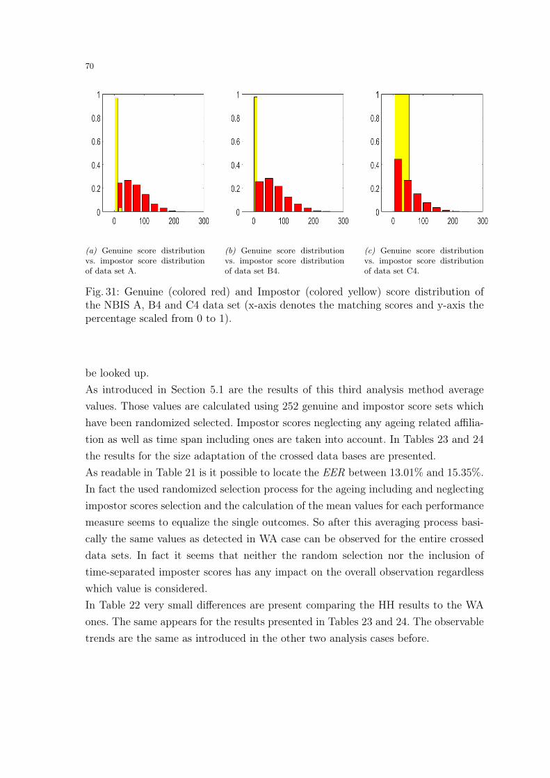
70





be looked up.As introduced in Section 5.1 are the results of this third analysis method averagevalues. Those values are calculated using 252 genuine and impostor score sets whichhave been randomized selected. Impostor scores neglecting any ageing related affilia-tion as well as time span including ones are taken into account. In Tables 23 and 24the results for the size adaptation of the crossed data bases are presented.As readable in Table 21 is it possible to locate the EER between 13.01% and 15.35%.In fact the used randomized selection process for the ageing including and neglectingimpostor scores selection and the calculation of the mean values for each performancemeasure seems to equalize the single outcomes. So after this averaging process basi-cally the same values as detected in WA case can be observed for the entire crosseddata sets. In fact it seems that neither the random selection nor the inclusion oftime-separated imposter scores has any impact on the overall observation regardlesswhich value is considered.In Table 22 very small differences are present comparing the HH results to the WAones. The same appears for the results presented in Tables 23 and 24. The observabletrends are the same as introduced in the other two analysis cases before.

71


single sets


crossed sets

C1 13.01 0.9239 47.61 6.71

C2 15.35 0.9141 44.71 6.64

C3 13.52 0.9225 43.81 6.80

C4 13.47 0.9285 49.06 6.57

C5 13.69 0.9242 48.65 6.55

Table 21: Characteristic individual performance values of NBIS matching includingEER, AUC, average genuine score and average impostor score using the HH method.

Even the Zero FAR decrease for data set C4 can be detected again. On the one handthis could be caused by the fact that ageing has no impact on the performed impostormatches. On the other hand it is also possible to conclude a relationship to the usedmatcher. As described in the previous WA and OA analysis are the matching scoresprovided by the used NBIS matcher more or less equal in each possible case and quitelow as well. For this purpose it could be that the performance of the matcher is alsoan important aspect in terms of ageing effects in fingerprint recognition. Suggestingthe assumption a better performing fingerprint matcher can not be influenced by age-ing that much as a worse one could be. This will be verified in the following sectionsdiscussing the other recognition results.

72


single sets


crossed sets

C1 0.2593 0.3598 0.5524 1.0

C2 0.2918 0.3911 0.5762 1.0

C3 0.2916 0.3903 0.8533 1.0

C4 0.2556 0.3460 0.8684 1.0

C5 0.2642 0.3447 0.9242 1.0

Table 22: Characteristic individual performance values of NBIS matching includingFAR100, FAR1000, Zero FAR and Zero FRR using the HH method.



C1 12.82 0.9239 47.56 6.58

C2 14.79 0.9141 44.69 6.51

C3 14.10 0.9225 43.84 6.71

C4 13.15 0.9285 49.07 6.52

C5 13.38 0.9246 48.74 6.50

Table 23: Characteristic individual performance values of NBIS matching includingEER, average genuine and impostor scores concerning the randomized splitted datasets using the HH method.

73



C1 0.2592 0.3509 0.5345 1.0

C2 0.2931 0.3812 0.5667 1.0

C3 0.2912 0.3793 0.7544 1.0

C4 0.2509 0.3448 0.6076 1.0

C5 0.2505 0.3422 0.7130 1.0

Table 24: Characteristic individual performance values of NBIS matching includingFAR100, FAR1000, Zero FAR and Zero FRR concerning concerning the randomizedsplitted data sets using the HH method.

5.3 NEURO

Regarding the WA, OA and HH analysis method for the matching results the pre-sentation of the NEURO related outcomes is splitted into four parts like it was donein the NBIS related part above. For this purpose all scores will be used for the firstcalculations. The results are presented in Table 25 and 26 and reveal more or less thesame genuine score degradation like introduced in the first minutiae based method.Furthermore the EER is increasing comparing single and crossed data sets and alsoAUC, FAR100, FAR1000 and Zero FAR reveal an identical tendency as in the NBIScase. For the average impostor and Zero FRR the same stability can be measuredas well. It seems that the same assumption ageing is influencing the genuine scores’behavior can be verified once more. But after getting an first impression about theperformance of the NEURO software the other analysis strategies WA, OA and HHwill be taken into account and a detailed discussion is performed.

NEURO WA Method: Regarding the results presented in the following Tables 27,28, 29, 30, 31 and 32, the overall tendency of outcomes is quite similar to the NBISanalysis displayed in the previous Section 5.2.

Looking at the matching performance in detail those results clearly show the bestmeasurements of all used matchers. For the single data sets the values can are be-

74

Data Set EER (%) AUC Av. Gen. Score Av. Imp. Score

single sets

A 2.07 0.9787 508.56 0.0055

B1 3.17 0.9677 499.66 0.0019

B2 1.96 0.9798 562.11 0.0054

B3 4.00 0.9595 464.01 0.0296

B4 2.04 0.9791 553.72 0.0134

B5 3.69 0.9626 484.50 0.0213

crossed sets

C1 5.32 0.9466 356.57 0.0028

C2 5.97 0.9402 359.21 0.0057

C3 6.16 0.9382 350.87 0.0151

C4 5.81 0.9418 368.43 0.0065

C5 6.72 0.9326 352.25 0.0087

Table 25: Characteristic individual performance values of NEUROmatching includingEER, AUC, Average Genuine Score and Average Impostor Score using all scores.

tween 1.96% and 4.00%. So the variation is nearly the same as in the NBIS results.For the crossed data bases outcomes an EER of 5.32% to 6.73% can be measured. Aswell as in the previous presented matcher performance it is also necessary to split theinput results to gather information that is able to be suitable compared to the singlesets. Therefore the EER for the 2old3new split can be confirmed as 5.31% to 6.75%

again. Nearly identical results can be posed in the 3old2new case. The interestinginformation beyond that is the fact that it seems that the EER is more stable as inthe NBIS performance looking at the single results. The absolute difference can bemeasured between 2.15% and 4.01%. Looking at the relative increase of B1/C1 andB2/C2 which are between 167.82% and 304.59% it gets clear that the first impres-sion of the stability is a matter of the chosen point of view. The single values andthe absolute difference of the EER values for the NEURO results are indeed lowercompared to the NBIS outcomes. Nevertheless the fluctuation concerning the relativeincrease of this performance characteristic is much higher compared to the results of

75

Data Set FAR100 FAR1000 Zero FAR Zero FRR

single sets

A 0.0414 0.0414 0.0824 1.0

B1 0.0635 0.0635 0.0790 1.0

B2 0.0392 0.0392 0.0563 1.0

B3 0.0799 0.0799 0.8084 1.0

B4 0.0408 0.0408 0.7341 1.0

B5 0.0737 0.0737 0.9825 1.0

crossed sets

C1 0.1064 0.1064 0.2215 1.0

C2 0.1193 0.1193 0.2582 1.0

C3 0.1232 0.1232 0.9026 1.0

C4 0.1162 0.1162 0.9064 1.0

C5 0.1345 0.1345 0.9956 1.0

Table 26: Characteristic individual performance values of NEUROmatching includingFAR100, FAR1000, Zero FAR and Zero FRR using all scores.


single sets


crossed sets

C1 5.32 0.9466 356.57 0.0037

C2 5.97 0.9402 359.21 0.0059

C3 6.16 0.9382 350.87 0.0173

C4 5.81 0.9418 368.43 0.0095

C5 6.73 0.9326 352.25 0.0131

Table 27: Characteristic individual performance values of NEURO matching includ-ing EER, AUC, Average Genuine Score and Average Impostor Score using the WAmethod.

76


single sets

same results as as in the all scores case

crossed sets

C1 0.1064 0.1064 0.2215 1.0

C2 0.1193 0.1193 0.2582 1.0

C3 0.1232 0.1232 0.9026 1.0

C4 0.1162 0.1162 0.9064 1.0

C5 0.1345 0.1345 0.9956 1.0

Table 28: Characteristic individual performance values of NEUROmatching includingFAR100, FAR1000, Zero FAR and Zero FRR using the WA method.

the other minutiae based fingerprint matcher.The information given in Tables 29, 30, 31 and 32 are confirming the outcomes pro-vided by the aforementioned tables. It can be detected that the decrease of the averagegenuine scores and the stability of the average impostor scores is present as in theother cases before. This identical tendency of those two measurements, like in theNBIS experimental results, can be confirmed basically for all considered characteris-tic values.

Focusing on the random selected and averaged data sets it is possible to verify theoverall performance as described. Looking at the outcomes displayed in Tables 33and 34, the following observation is detectable: In fact, there is not really a differenceto the original crossed data sets observable. It seems that apart from varied valuesthe same tendency is given. The most interesting observation which can be made isthe confirmation of the drop of the Zero FAR value for data set C4 like described inthe NBIS case as well. Compared to the NBIS results the same tendency for AUC,FAR100, FAR1000, Zero FAR and Zero FRR is observable. The Zero FRR seems tobe fixed at 1.0 once more, confirming the expected behavior. The only difference forFAR100 and FAR1000, which can measured, is that the difference between the valuesis not that high compared to NBIS.

77



C1 5.31 0.9467 367.79 0.0044

C2 5.88 0.9409 378.48 0.0068

C3 6.25 0.9372 351.54 0.0312

C4 5.41 0.9456 391.22 0.0143

C5 6.75 0.9322 360.96 0.0223

Table 29: Characteristic individual performance values of NEURO matching includ-ing EER, AUC, Average Genuine Score and Average Impostor Score concerning thesplitted data 2old3new using the WA method.

Nevertheless a short discussion about the average genuine and impostor scores willbe done in the following. The average genuine score for the single data sets is muchhigher than in the crossed data bases no matter taking the values of all imprints intoaccount or the splitted ones. Due to that fact the Figures 35 and 34 help to gathersome more information.The genuine score distribution for the 2009 imprints are delivering higher scores andcan be compared to something like a normal distribution. For the images from 2013

it is not possible to find a distribution the matching values look like. But for thecrossed set there can be the clear description that the distribution is similar to theNBIS case skewed to the right. So all in all there is the same tendency as in the otherminutiae based matcher. A shift to the left of the matching scores can be detected,caused by a reduction of the genuine scores of about 30 to 38 percent. This percentagecan be calculated using the genuine scores in Table 27 and divide for example theaverage genuine score of C1 by the average genuine score of the singe data set A. TheAUC results are also displaying the same tendency as detected in the NBIS case. Soa decrease for the crossed data bases compared to the single sets can be measured. Ingeneral it can be stated that there is hardly no difference in the tendency of the usedcharacteristic values of NBIS and NEURO. The crossed data sets’ EERis increasing,the same can be measured for FAR100, FAR1000 and Zero FAR. The average genuinescores are decreasing if the values from the single and crossed data bases are comparedand the average impostor scores and Zero FRR remain more or less stable.

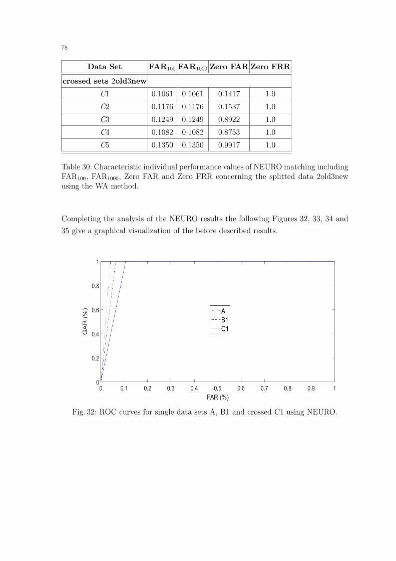
78



C1 0.1061 0.1061 0.1417 1.0

C2 0.1176 0.1176 0.1537 1.0

C3 0.1249 0.1249 0.8922 1.0

C4 0.1082 0.1082 0.8753 1.0

C5 0.1350 0.1350 0.9917 1.0

Table 30: Characteristic individual performance values of NEUROmatching includingFAR100, FAR1000, Zero FAR and Zero FRR concerning the splitted data 2old3newusing the WA method.

Completing the analysis of the NEURO results the following Figures 32, 33, 34 and35 give a graphical visualization of the before described results.

Fig. 32: ROC curves for single data sets A, B1 and crossed C1 using NEURO.

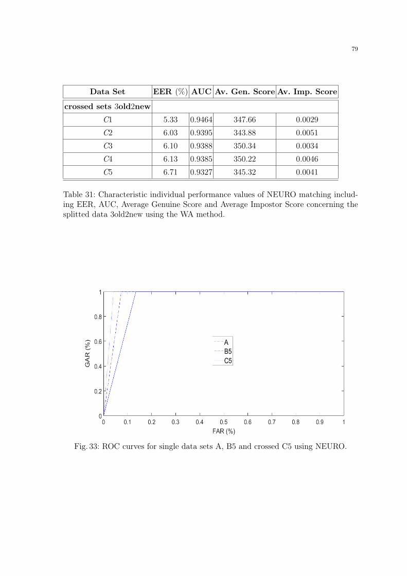
79



C1 5.33 0.9464 347.66 0.0029

C2 6.03 0.9395 343.88 0.0051

C3 6.10 0.9388 350.34 0.0034

C4 6.13 0.9385 350.22 0.0046

C5 6.71 0.9327 345.32 0.0041

Table 31: Characteristic individual performance values of NEURO matching includ-ing EER, AUC, Average Genuine Score and Average Impostor Score concerning thesplitted data 3old2new using the WA method.

Fig. 33: ROC curves for single data sets A, B5 and crossed C5 using NEURO.

80



C1 0.1067 0.1067 0.2266 1.0

C2 0.1206 0.1206 0.2581 1.0

C3 0.1219 0.1219 0.2435 1.0

C4 0.1225 0.1225 0.2335 1.0

C5 0.1342 0.1342 0.2420 1.0

Table 32: Characteristic individual performance values of NEUROmatching includingFAR100, FAR1000, Zero FAR and Zero FRR concerning the splitted data 3old2newusing the WA method.



C1 5.29 0.9465 356.93 0.0038

C2 5.98 0.9397 359.12 0.0060

C3 6.21 0.9373 350.21 0.0175

C4 5.75 0.9420 368.78 0.0095

C5 6.73 0.9321 352.36 0.0131

Table 33: Characteristic individual performance values of NEUROmatching includingEER, average genuine and impostor scores concerning the randomized splitted datasets using the WA method.

81



C1 0.1058 0.1058 0.1805 1.0

C2 0.1195 0.1195 0.2102 1.0

C3 0.1242 0.1242 0.8267 1.0

C4 0.1150 0.1150 0.5589 1.0

C5 0.1346 0.1346 0.7737 1.0

Table 34: Characteristic individual performance values of NEUROmatching includingFAR100, FAR1000, Zero FAR and Zero FRR concerning concerning the randomizedsplitted data sets using the WA method.




Fig. 34: Genuine (colored red) and Impostor (colored yellow) score distribution of theNEURO A, B2 and C2 data set (x-axis denotes the matching scores and y-axis thepercentage scaled from 0 to 1) using WA analysis.

82




Fig. 35: Genuine (colored red) and Impostor (colored yellow) score distribution of theNEURO A, B3 and C3 data set (x-axis denotes the matching scores and y-axis thepercentage scaled from 0 to 1) using WA analysis.

NEURO OA Method: In the following Section 5.3 the results of using only im-postor scores including the 4 year time span are presented. In Tables 35 and 36 thecharacteristic values without any data set size adaption can be looked up.

In fact there is not really a difference measurable comparing the characteristic valuesof the OA analysis and those from the WA analysis of the previous section. The onlydifference is a small change in the average impostor scores. The average scores are alittle bit lower as for the corresponding ones in the WA case. Despite an interestingobservation can be made looking at data set C4 and the Zero FAR. As introduced inthe OA analysis of the NBIS results the reduction of this value can be detected oncemore. So the assumption that the drop could be a matter of the used matcher canbe devitalized. It remains to be seen if the same effect occurs for the non-minutiaematchers as well. It could be that it is based on the used minutiae strategy. Be-cause there was not really a difference to the results of the WA method it is likelythat for the following randomly size adapted analysis also the same stability can bedetected. The calculated values of the size adaption are presented in Tables 37 and 38.

83


single sets


crossed sets

C1 5.32 0.9466 356.57 0.0019

C2 5.97 0.9402 359.21 0.0055

C3 6.16 0.9382 350.87 0.0128

C4 5.81 0.9418 368.43 0.0036

C5 6.72 0.9326 352.25 0.0044

Table 35: Characteristic individual performance values of NEURO matching includ-ing EER, AUC, Average Genuine Score and Average Impostor Score using the OAmethod.

Looking at the results the presumption of almost no changes can be verified. Espe-cially for EER, AUC, average genuine scores average impostor scores and Zero FRRa high amount of similarity is present. The probably most interesting aspect is thatFAR100 and FAR1000 outcomes tend to stay identical whereas the Zero FAR is themost fluctuating value of the whole OA analysis for the NEURO results. These spe-cific results for the randomized crossed sets are lowest for all considered Zero FARvalues so far. Therefore it could be worthwhile to have a look on this trend in thefollowing HH analysis part.

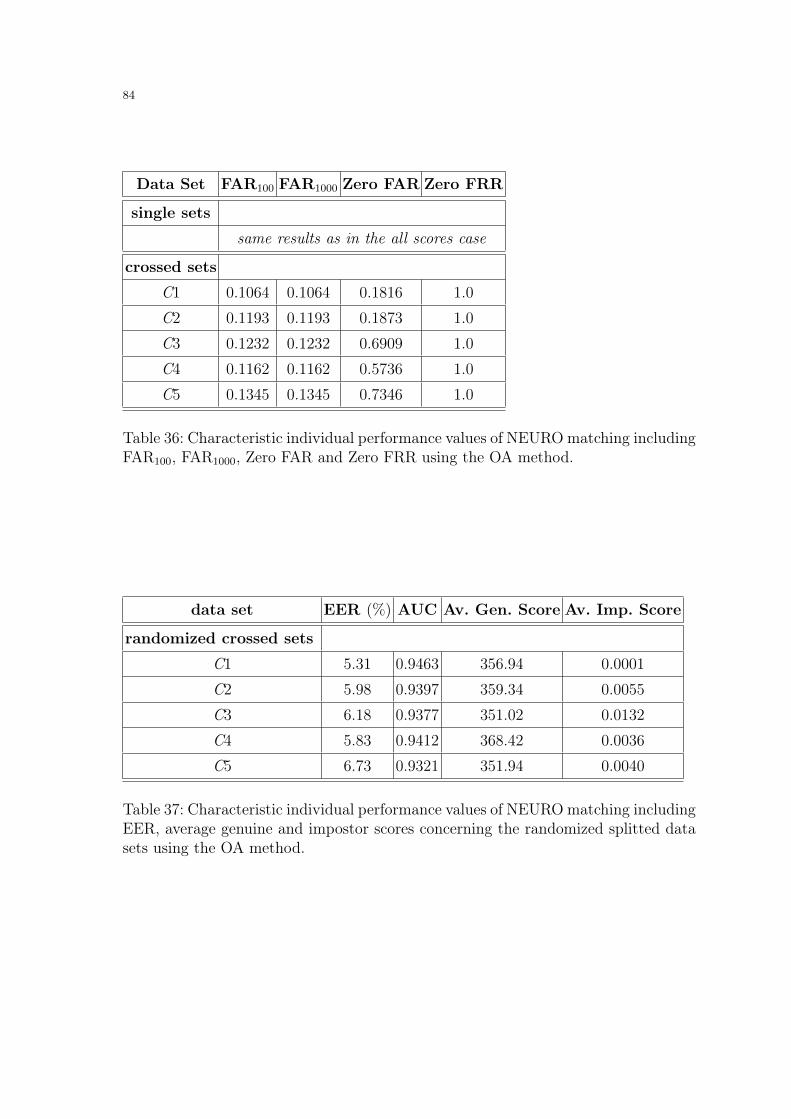
84


single sets


crossed sets

C1 0.1064 0.1064 0.1816 1.0

C2 0.1193 0.1193 0.1873 1.0

C3 0.1232 0.1232 0.6909 1.0

C4 0.1162 0.1162 0.5736 1.0

C5 0.1345 0.1345 0.7346 1.0

Table 36: Characteristic individual performance values of NEUROmatching includingFAR100, FAR1000, Zero FAR and Zero FRR using the OA method.



C1 5.31 0.9463 356.94 0.0001

C2 5.98 0.9397 359.34 0.0055

C3 6.18 0.9377 351.02 0.0132

C4 5.83 0.9412 368.42 0.0036

C5 6.73 0.9321 351.94 0.0040

Table 37: Characteristic individual performance values of NEUROmatching includingEER, average genuine and impostor scores concerning the randomized splitted datasets using the OA method.

85



C1 0.1062 0.1062 0.1521 1.0

C2 0.1195 0.1195 0.1648 1.0

C3 0.1235 0.1235 0.5773 1.0

C4 0.1165 0.1165 0.3592 1.0

C5 0.1346 0.1346 0.4475 1.0

Table 38: Characteristic individual performance values of NEUROmatching includingFAR100, FAR1000, Zero FAR and Zero FRR concerning concerning the randomizedsplitted data sets using the OA method.

NEURO HH Method: The final presentation of the missing third part of theNEURO matching score analysis will be displayed in this section of the master thesis.The results described in Tables 39 and 40 are representing the performance charac-teristics of the entire used data set, while the size adapted analysis can be looked upin Tables 41 and 42.

Basically all results which can be looked up in Tables 39, 40, 41 and 42 are more orless same as before in OA and WA analysis. So once more a clear observable stabilityof average impostor scores and a decrease in terms of AUC, average genuine scores,FAR100, FAR1000 and Zero FAR can be described comparing the single and crosseddata sets’ results. An identical increase of the EER is detectable as well. The varietyof all NEURO based results is more similar to each other compared to the outcomespresented in Section 5.3. There will not be a detailed description of the single valuesbecause this has been done in the aforementioned WA analysis and there are no realdifferences to those outcomes. Basically it seems that neither the random selectionnor the inclusion of time-separated imposter scores has any impact on the overallobservation. The shift of the genuine score distribution based on an approximationtoward the impostor score distribution can be detected in WA, OA and HH analysisindependently.In Figure 36 it can be verified that the difference between this figure and Figure 34

86


single sets


crossed Sets

C1 5.32 0.9466 356.57 0.0038

C2 5.97 0.9402 359.21 0.0061

C3 6.16 0.9382 350.87 0.0173

C4 5.81 0.9418 368.43 0.0091

C5 6.73 0.9326 352.25 0.0129

Table 39: Characteristic individual performance values of NEURO matching includ-ing EER, AUC, Average Genuine Score and Average Impostor Score using the HHmethod.

using the same data base can hardly be seen except for one bar of the histogram inthe right column.




Fig. 36: Genuine (colored red) and Impostor (colored yellow) score distribution of theNEURO A, B2 and C2 data set (x-axis denotes the matching scores and y-axis thepercentage scaled from 0 to 1) using HH analysis.

87


single sets


crossed Sets

C1 0.1064 0.1064 0.2050 1.0

C2 0.1193 0.1193 0.2321 1.0

C3 0.1232 0.1232 0.8798 1.0

C4 0.1162 0.1162 0.7179 1.0

C5 0.1345 0.1345 0.9301 1.0

Table 40: Characteristic individual performance values of NEUROmatching includingFAR100, FAR1000, Zero FAR and Zero FRR using the HH method.



C1 5.33 0.9462 356.95 0.0029

C2 6.00 0.9394 359.12 0.0058

C3 6.16 0.9379 350.82 0.0151

C4 5.80 0.9414 368.33 0.0066

C5 6.71 0.9323 352.39 0.0092

Table 41: Characteristic individual performance values of NEUROmatching includingEER, average genuine and impostor scores concerning the randomized splitted datasets using the HH method.

88



C1 0.1066 0.1066 0.1713 1.0

C2 0.1200 0.1200 0.1874 1.0

C3 0.1231 0.1231 0.7153 1.0

C4 0.1160 0.1160 0.4452 1.0

C5 0.1342 0.1342 0.6410 1.0

Table 42: Characteristic individual performance values of NEUROmatching includingFAR100, FAR1000, Zero FAR and Zero FRR concerning concerning the randomizedsplitted data sets using the HH method.

5.4 FC

The following results represent the performance of the first non minutiae based fin-gerprint matcher. The calculated matching scores differ from the before describedminutiae based outcomes. The described outcomes are based on the WA analysismethod. In Tables 43 and 44 the most important performance values can be lookedup. It seems that there must be a failure each time when the 2009 data set is involvedin the matching process. In fact the EER of the single 2009 and crossed 2009 calcula-tions are the worst of all performed. So for example an EER of 55.68% is even worsethan bet on tossing a coin.

Based on the results there is a second effect observable. The EER of the 2013 singledata sets is located around 12% for the B2 and B4 data set and respectively between16% and 18% for the other three data bases. Those are interesting outcomes becausethe impression of the first results could be that there is something wrong with theimplementation or with the used method itself. But it seems that there must be an-other reason why the matcher is delivering such bad results on the one hand and onthe other hand EER values that are more or less in a realistic range.Looking at the performance values more precisely there is a tendency within thesplitted crossed data bases. The 2old3new data sets gather the worst results. The

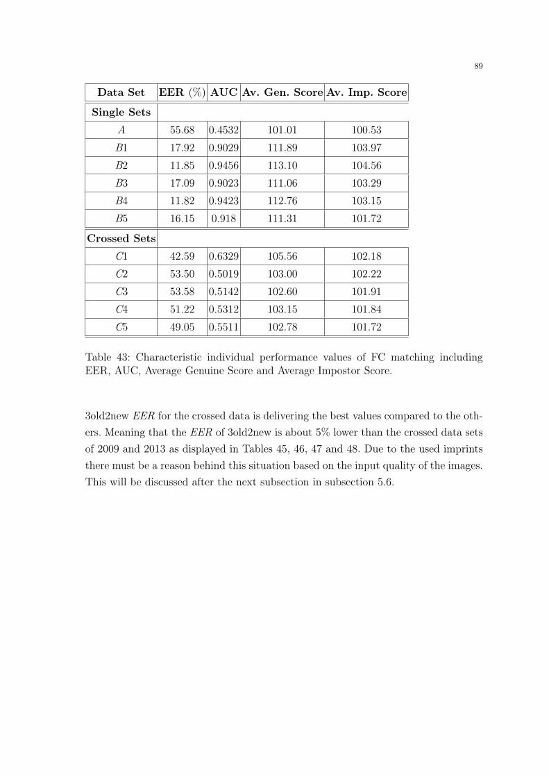
89


Single Sets

A 55.68 0.4532 101.01 100.53

B1 17.92 0.9029 111.89 103.97

B2 11.85 0.9456 113.10 104.56

B3 17.09 0.9023 111.06 103.29

B4 11.82 0.9423 112.76 103.15

B5 16.15 0.918 111.31 101.72

Crossed Sets

C1 42.59 0.6329 105.56 102.18

C2 53.50 0.5019 103.00 102.22

C3 53.58 0.5142 102.60 101.91

C4 51.22 0.5312 103.15 101.84

C5 49.05 0.5511 102.78 101.72

Table 43: Characteristic individual performance values of FC matching includingEER, AUC, Average Genuine Score and Average Impostor Score.

3old2new EER for the crossed data is delivering the best values compared to the oth-ers. Meaning that the EER of 3old2new is about 5% lower than the crossed data setsof 2009 and 2013 as displayed in Tables 45, 46, 47 and 48. Due to the used imprintsthere must be a reason behind this situation based on the input quality of the images.This will be discussed after the next subsection in subsection 5.6.

90


Single Sets

A 0.9436 0.9976 1.0 0.9862

B1 0.3617 0.9083 1.0 0.7342

B2 0.1547 0.8402 1.0 0.6816

B3 0.3664 0.9281 1.0 0.7362

B4 0.1599 0.8581 1.0 0.6296

B5 0.2886 0.8524 1.0 0.9383

Crossed Sets

C1 0.8939 0.9914 1.0 0.9136

C2 0.9562 0.9978 1.0 0.9395

C3 0.9488 0.9965 1.0 0.9679

C4 0.9444 0.9962 1.0 0.9337

C5 0.9350 0.9960 1.0 0.9949

Table 44: Characteristic individual performance values of FC matching includingFAR100, FAR1000, Zero FAR and Zero FRR.


Crossed Sets 2old3new

C1 45.66 0.5938 104.42 102.14

C2 58.83 0.4298 101.61 102.75

C3 56.93 0.4578 101.41 101.89

C4 55.38 0.4732 101.83 101.79

C5 51.95 0.5074 101.61 100.94

Table 45: Characteristic individual performance values of FC matching includingEER, AUC, Average Genuine Score and Average Impostor Score concerning the split-ted data 2old3new.

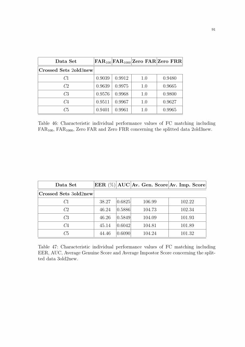
91



C1 0.9039 0.9912 1.0 0.9480

C2 0.9639 0.9975 1.0 0.9665

C3 0.9576 0.9968 1.0 0.9800

C4 0.9511 0.9967 1.0 0.9627

C5 0.9401 0.9961 1.0 0.9965

Table 46: Characteristic individual performance values of FC matching includingFAR100, FAR1000, Zero FAR and Zero FRR concerning the splitted data 2old3new.



C1 38.27 0.6825 106.99 102.22

C2 46.24 0.5886 104.73 102.34

C3 46.26 0.5849 104.09 101.93

C4 45.14 0.6042 104.81 101.89

C5 44.46 0.6090 104.24 101.32

Table 47: Characteristic individual performance values of FC matching includingEER, AUC, Average Genuine Score and Average Impostor Score concerning the split-ted data 3old2new.

92



C1 0.8708 0.9911 1.0 0.8270

C2 0.9453 0.9980 1.0 0.8783

C3 0.9342 0.9963 1.0 0.9270

C4 0.9345 0.9957 1.0 0.8668

C5 0.9227 0.9962 1.0 0.9056

Table 48: Characteristic individual performance values of FC matching includingFAR100, FAR1000, Zero FAR and Zero FRR concerning the splitted data 3old2new.

5.5 POC

Regarding to the second non minutiae based matching results there is a huge dif-ference between the minutiae based outcomes once again using the WA analysisstrategy. First of all it is very interesting to consider the EER values of the databases. Roughly spoken, similar to the minutiae matcher results a correlation betweenthe non minutiae matcher results can be spotted. That means that for the POC theEER results are quite similar to the values from FC. The EER for the single datasets from 2013 is allocated between 22 and 26 percent. But each time imprints from2009 are included in a data base they are distributed from 40 to 46. The differenceof the worst results, delivered by the A again, is even larger than before. Here thegap between the crossed sets and the single set from 2009 is almost 3%. The over-all calculated values can be looked up in the following Tables 49, 50, 51, 52, 53 and 54.

For this purpose the EER values for the split data sets are rather diverse. Forthe 2old3new case the results are oscillating between 29 and 35 percent whereasin 3old2new they get even worse than the 2009 single EER namely 46% to nearly49%. Because of this situation it is not sure to argue if there is a similar shift to theleft within the genuine score distribution like in the minutiae based matcher results.Furthermore the outcomes confirm the unexpected jump in the Zero FRR values lo-cated in the minutiae based matchers to be an abnormality related to those matcher

93


Single Sets

A 46.11 0.5665 0.1119 0.0812

B1 26.06 0.7842 0.2365 0.0810

B2 22.66 0.8082 0.2567 0.0828

B3 25.03 0.7911 0.2449 0.0820

B4 22.61 0.8077 0.2875 0.0838

B5 24.87 0.7919 0.2532 0.0858

Crossed Sets

C1 40.11 0.6626 0.1442 0.0812

C2 41.74 0.6570 0.1527 0.0820

C3 43.12 0.6427 0.1489 0.0816

C4 40.68 0.6688 0.1641 0.0825

C5 40.49 0.6674 0.1552 0.0835

Table 49: Characteristic individual performance values of POC matching includingEER, AUC, Average Genuine Score and Average Impostor Score.

types and the data. But there is another interesting fact concerning the Zero FAR.It seems that this value is stable over all data sets and more or less fixed at 0.7614without any detectable reason. It is also necessary to discuss the FAR100 and FAR1000

outcomes because at the chosen observation values it was not possible to gather anyinformation because the lowest FAR values that can be taken into account are greaterthan those values.Finally it is clear that there must be the same problem included as in the FC match-ing results. In the following Section 5.6 this situation will be discussed into moredetail.

5.6 Variability of data sets and 2. non minutiae experiments

Regarding the displayed results in Section 5.2 there are a few interesting observationsthat need to be discussed. The most important one is the quite bad performance ofthe non minutiae based matchers FC and POC.

94


Single Sets

A - - 0.7614 0.9413

B1 - - 0.7613 0.7031

B2 - - 0.7614 0.6332

B3 - - 0.7614 0.6097

B4 - - 0.7614 0.6995

B5 - - 0.7614 0.6760

Crossed Sets

C1 0.7602 0.7614 0.7614 0.9083

C2 0.7606 0.7614 0.7614 0.8909

C3 0.7602 0.7614 0.7614 0.8742

C4 0.7602 0.7614 0.7614 0.9125

C5 0.7614 0.7614 0.7614 0.9023

Table 50: Characteristic individual performance values of POC matching includingFAR100, FAR1000, Zero FAR and Zero FRR.



C1 31.24 0.7910 0.1916 0.0801

C2 33.79 0.7723 0.2013 0.0816

C3 35.31 0.7518 0.1937 0.0810

C4 28.48 0.8237 0.2312 0.0820

C5 29.72 0.8102 0.2112 0.0832

Table 51: Characteristic individual performance values of POC matching includingEER, AUC, Average Genuine Score and Average Impostor Score concerning the split-ted data 2old3new.

95



C1 0.5974 0.7494 0.7614 0.8245

C2 0.6632 0.7551 0.7614 0.8398

C3 0.6862 0.7544 0.7614 0.7888

C4 0.6077 0.7490 0.7614 0.7638

C5 0.6251 0.7612 0.7614 0.8163

Table 52: Characteristic individual performance values of POC matching includingFAR100, FAR1000, Zero FAR and Zero FRR concerning the splitted data 2old3new.



C1 46.45 0.5559 0.1064 0.0822

C2 47.28 0.5638 0.1137 0.0824

C3 48.61 0.5533 0.1130 0.0823

C4 48.31 0.5421 0.1103 0.0830

C5 47.80 0.5514 0.1105 0.0838

Table 53: Characteristic individual performance values of POC matching includingEER, AUC, Average Genuine Score and Average Impostor Score concerning the split-ted data 3old2new.

On the one hand the results in terms of EER and average genuine and impostorscores seems to be realistic in case of looking at the CASIA 2013 data sets. For sure,for example the EER is not that good compared to the minutiae based methods butthe values range in the same area as in [17].On the other hand each data set where the CASIA 2009 images are included isperforming bad for those two matcher methodologies. There is not a big differencebetween tossing a coin and finding the corresponding imprints because the EER canbe located around 40% in case of the POC method and around 55% for the FCmatcher.

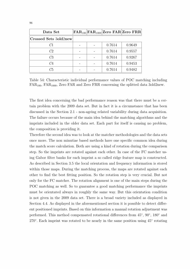
96



C1 - - 0.7614 0.9649

C2 - - 0.7614 0.9557

C3 - - 0.7614 0.9267

C4 - - 0.7614 0.9453

C5 - - 0.7614 0.9482

Table 54: Characteristic individual performance values of POC matching includingFAR100, FAR1000, Zero FAR and Zero FRR concerning the splitted data 3old2new.

The first idea concerning the bad performance reason was that there must be a cer-tain problem with the 2009 data set. But in fact it is a circumstance that has beendiscussed in the Section 2.1 - non-ageing related variability during data acquisition.The failure occurs because of the main idea behind the matching algorithms and theimprints included in the older data set. Each part for itself is causing no problem,the composition is providing it.Therefore the second idea was to look at the matcher methodologies and the data setsonce more. The non minutiae based methods have one specific common idea duringthe match score calculation. Both are using a kind of rotation during the comparisonstep. So the imprints are rotated against each other. In case of the FC matcher us-ing Gabor filter banks for each imprint a so called ridge feature map is constructed.As described in Section 3.5 the local orientation and frequency information is storedwithin those maps. During the matching process, the maps are rotated against eachother to find the best fitting position. So the rotation step is very crucial. But notonly for the FC matcher. The rotation alignment is one of the main steps during thePOC matching as well. So to guarantee a good matching performance the imprintsmust be orientated always in roughly the same way. But this orientation conditionis not given in the 2009 data set. There is a broad variety included as displayed inSection 4.4. As displayed in the aforementioned section it is possible to detect differ-ent positioned imprints. Based on this information a manual rotation adjustment wasperformed. This method compensated rotational differences from 45◦, 90◦, 180◦ and270◦. Each imprint was rotated to be nearly in the same position using 45◦ rotating

97

steps. To be on the safe side the same adaption was also performed for some imagesin the 2013 data sets too. The rotated imprints can be located after this rotation stepwithin a angle of 40◦. This specific area is the rotation range that is covered by therotation step of the non minutiae matching methods.

So after the adjustment step the matching calculation for POC and FC were per-formed once again. For the non minutiae based matcher there was no need to repeatthe experiments due to the fact that the this method is, due to the minutiae features,rotation independent.During the calculation step another failure occurred for the FC method. As describedin Chapter 4 the image width is 328 pixel and the height 356 pixel. According to themanual rotation not all imprints have a resolution of 328x356 anymore. There area lot of images the measurement of which have been flipped to 356x328. Thereforethe implementation is not able to compare both kinds of images. All imprints musthave the same dimensions to provide a correct ridge feature map comparison. To en-sure perfect functioning, all images dimensions have been equalized to 328x328. Thisis possible because each imprint contains a lot of information that is not useful forthe comparison because the surface of the sensor is acquired. Those parts were cut off.

In the following two Sections 5.7 and 5.8 the results of the second experiments con-cerning the FC and POC fingerprint recognition system will be described. Basicallyan identical analysis was performed as introduced in Section 5.1. So for both exper-iments AS, WA, OA and HH analysis method are used to describe the results intomore detail.

5.7 2. FC Experiments:

The presentation of the 2. FC and POC experiments will be done in the same manneras the results for the minutiae based matcher has been performed. So at first there willbe the discussion based on the results without using the ageing influenced impostorscores and afterward those scores were added and the OA and HH analysis will bedescribed. But before the corresponding outcomes of the entire data sets are presentedin Tables 55 and 56. Similar to the minutiae based outcomes a degradation of theaverage genuine scores of the crossed sets is observable. Furthermore there is one

98

variation included as well. The difference between the average genuine scores of thesingle and crossed data bases is smaller as for NBIS and NEURO. Looking at theother results basically a very similar situation as for the minutiae based fingerprintrecognition systems can be described. Nevertheless it is possible to observe that themanual rotation alignment improved the performance a lot comparing the values withthe first experiments. But a clear difference between data set A and the other singlesets remains. This effect is present for nearly all measurements. It is based on thecircumstance that much more rotational displacement was included in the imprintscontained in data base A. Furthermore this will certainly have an impact on thecrossed data measurements as well. So all results are biased by this rotation causedeffect which influences a precise comparison with the minutiae based recognitionsystems as well. In general the same average genuine score degradation is causing theEER increase comparing single data bases and crossed ones. AUC decreases, FAR100,FAR1000 and Zero FAR tend to increase. Additionally is the stability of the averageimpostor scores and Zero FRR confirming as well that the second experiments behavelike expected. The detailed discussion can be looked up in the following descriptionsof WA, OA and HH analysis.

FC WA Method: The results for the second FC experiments and in particular thecorresponding without ageing impostor score analysis will be displayed in the follow-ing Tables 57 and 58. It is clearly observable that the manual rotation adjustmentcaused a much better performance then during the first experiments. The EER of the2013 data sets remain almost stable. Due to a few rotation adjustments within thosedata sets a slight difference is detectable but not crucial. The EER of the beforehandworse performing data bases was more than halved. The outcomes are now locatedbetween 20.17% and 29.24% in the data sets containing imprints from 2009.According to the EER results of the 2. FC experiments it is necessary to discussthose values into more detail. At first view only the same tendency as detected in theminutiae based matching results can be observed. But, it is decisive that the impactof the high non-ageing related variability within the given data sets is influencing thematching results, even after performing the rotation alignment step discussed before.Therefore lets have a look at for example data set B2 and data set C2. The relativeincrease of the EER in the NBIS results for these two data bases is around 188%.The relative increase based on the NEURO outcomes is around 304%. The relative

99


Single Sets

A 23.86 0.8192 110.24 102.03

B1 17.13 0.8928 113.18 104.62

B2 12.20 0.9427 113.10 104.67

B3 17.32 0.8987 111.06 103.50

B4 11.72 0.9450 112.56 102.80

B5 16.73 0.9086 111.11 102.21

Crossed Sets

C1 20.15 0.8329 112.81 102.13

C2 27.23 0.8073 108.72 102.67

C3 25.70 0.8219 108.52 102.44

C4 25.66 0.8233 108.62 102.19

C5 27.21 0.8071 108.12 102.00

Table 55: Characteristic individual performance values of FC matching includingEER, AUC, Average Genuine Score and Average Impostor Score using all matchingscores.

values for the FC matcher is around 239%. So depending on this data set the relativeincrease of the EER in FC is higher compared to the results from NBIS but evenlower as for the NEURO case. It will be interesting to see if in the POC outcomesthe same effect can be displayed. Especially because the absolute increase for thefirst non-minutiae matcher is located between 3.04% and 17.04%. So a much highervariability can be detected as for the minutiae based approaches.

While the EER is higher for the crossed data bases, the AUC is decreasing comparedto the single data sets. The same increase as for the EER can be observed for FAR100,FAR1000 and Zero FAR as well. During the 2old3new, 3old2new and also the random-ized averaging size adaptation computations the same tendencies could be confirmed.Especially looking at the average genuine score tendency leads to the assumptionthat also the shift in the genuine and impostor score distribution like observed in the

100


Single Sets

A 0.5331 0.6551 0.8352 1.0

B1 0.3698 0.4948 0.6592 1.0

B2 0.3326 0.4801 0.6612 1.0

B3 0.4091 0.5969 0.7376 1.0

B4 0.2637 0.4071 0.7071 1.0

B5 0.3785 0.5285 0.9663 1.0

Crossed Sets

C1 0.4317 0.5321 0.6861 1.0

C2 0.6539 0.7741 0.9191 1.0

C3 0.6488 0.7873 0.9496 1.0

C4 0.6252 0.7555 0.9223 1.0

C5 0.6522 0.7761 0.9984 1.0

Table 56: Characteristic individual performance values of FC matching includingFAR100, FAR1000, Zero FAR and Zero FRR using all matching scores.


single sets


Crossed Sets

C1 20.17 0.8319 112.81 102.19

C2 29.24 0.7849 108.72 103.29

C3 26.91 0.8097 108.52 102.83

C4 25.92 0.8204 108.62 102.33

C5 27.07 0.8088 108.12 101.94

Table 57: Characteristic individual performance values of FC matching includingEER, AUC, Average Genuine Score and Average Impostor Score using WA analysis.

101


single sets


Crossed Sets

C1 0.4253 0.5285 0.6613 1.0

C2 0.6750 0.7890 0.9191 1.0

C3 0.6518 0.7860 0.9496 1.0

C4 0.6238 0.7551 0.9223 1.0

C5 0.6454 0.7727 0.9984 1.0

Table 58: Characteristic individual performance values of FC matching includingFAR100, FAR1000, Zero FAR and Zero FRR using WA analysis.

minutiae based matcher results can be stated as well in the FC case. The results ofthe 2old3new, 3old2new and the averaging computations can be looked up in Tables59, 60, 61, 62, 63 and 64.Looking at the average impostor and genuine scores the difference between the resultsof the first experiments is also detectable. While the outcomes for the impostor scoresdid not change significantly, the genuine scores raised in those data bases where im-prints from 2009 are included. The same tendency is observable for the AUC valuesas well. So the AUC is now almost stable comparing the single data sets with eachother. Additionally a more detailed information concerning the FAR100 and FAR1000

can be described. Two examples of ROC, also displaying AUC, can be looked up inFigures 37 and 38.

Similar like in the NBIS and NEURO results it seems that the growing process fromFAR100 to Zero FAR can be compared with the tendency observable in the minutiaematching processes. Of course the difference between FAR100 and FAR1000 is muchhigher and the deviation between FAR100, FAR1000 and Zero FAR is much lower forthis FC case compared to NBIS or NEURO. The increase of the FAR100 values fromsingle to crossed data sets is also much bigger, but all in all the same tendency canbe stated. Besides, a cross-sensor effect concerning the T2 sensor data sets B1 and

102



C1 21.20 0.8281 112.41 102.28

C2 32.03 0.7518 108.14 103.52

C3 27.76 0.7973 108.24 102.90

C4 27.78 0.7994 108.20 102.53

C5 27.75 0.8020 107.84 101.85

Table 59: Characteristic individual performance values of FC matching includingEER, AUC, Average Genuine Score and Average Impostor Score concerning the split-ted data 2old3new using WA analysis.

C1 displayed in Table 57 is detectable. Especially looking at the EER outcomes it isclearly visible that there must be an impact because the values are definitely lowercompared to the other data sets. It is interesting that this cross-sensor effect existsfor the FC outcomes. For the minutiae based matcher the same did not occure. Soprobably it is matcher based and therefore just detectable for the FC results. Addi-tionally it must be mentioned that the described drop of the Zero FAR for data setC4 seems to be based on NBIS and NEURO results. For the remaining analysis ofthe second non-minutiae matcher these aspects will be discussed as well.

As displayed in Figures 39 and 40 a similar shift of the genuine score distribution tothe left can be detected. It is clear that this shift is not that large as in the minutiaebased results but nevertheless it is clearly visible. The difference to the uniquenessof the minutiae based method can be explained looking at the average genuine andimpostor score values. They are much more similar to each other compared to theNBIS and NEURO matching results. The difference between the impostor scores andgenuine scores for the crossed data sets is smaller then in the single data sets. Thiseffect can be explained due to the not so clear distinctive matching results. It will beinteresting to see how far these circumstances will be important in the OA and HHanalysis and also in Chapter 6.

103



C1 0.4300 0.5424 0.6320 1.0

C2 0.7228 0.8322 0.9414 1.0

C3 0.6669 0.8032 0.9559 1.0

C4 0.6389 0.7734 0.9430 1.0

C5 0.6579 0.7910 0.9991 1.0

Table 60: Characteristic individual performance values of FC matching includingFAR100, FAR1000, Zero FAR and Zero FRR concerning the splitted data 2old3newusing WA analysis.

Fig. 37: ROC curves for single data sets A, B2 and crossed C2 using FC WA analysis.

104



C1 19.33 0.8361 113.31 102.11

C2 25.91 0.8225 109.44 103.05

C3 25.74 0.8243 108.86 102.75

C4 23.71 0.8435 109.15 102.17

C5 26.06 0.8182 108.46 102.04

Table 61: Characteristic individual performance values of FC matching includingEER, AUC, Average Genuine Score and Average Impostor Score concerning the split-ted data 3old2new using WA analysis.



C1 0.4158 0.5061 0.6321 1.0

C2 0.6165 0.7329 0.8612 1.0

C3 0.6293 0.7650 0.9107 1.0

C4 0.6012 0.7252 0.8772 1.0

C5 0.6308 0.7505 0.8989 1.0

Table 62: Characteristic individual performance values of FC matching includingFAR100, FAR1000, Zero FAR and Zero FRR concerning the splitted data 3old2newusing WA analysis.

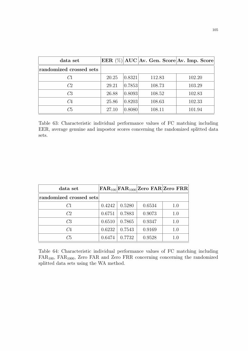
105



C1 20.25 0.8321 112.83 102.20

C2 29.21 0.7853 108.73 103.29

C3 26.88 0.8093 108.52 102.83

C4 25.86 0.8203 108.63 102.33

C5 27.10 0.8080 108.11 101.94

Table 63: Characteristic individual performance values of FC matching includingEER, average genuine and impostor scores concerning the randomized splitted datasets.



C1 0.4242 0.5280 0.6534 1.0

C2 0.6751 0.7883 0.9073 1.0

C3 0.6510 0.7865 0.9347 1.0

C4 0.6232 0.7543 0.9169 1.0

C5 0.6474 0.7732 0.9528 1.0

Table 64: Characteristic individual performance values of FC matching includingFAR100, FAR1000, Zero FAR and Zero FRR concerning concerning the randomizedsplitted data sets using the WA method.

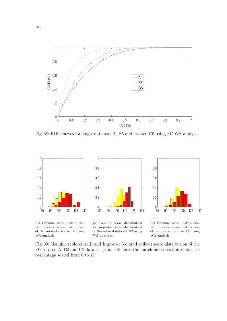
106

Fig. 38: ROC curves for single data sets A, B5 and crossed C5 using FC WA analysis.

(a) Genuine score distributionvs. impostor score distributionof the rotated data set A usingWA analysis.

(b) Genuine score distributionvs. impostor score distributionof the rotated data set B2 usingWA analysis.

(c) Genuine score distributionvs. impostor score distributionof the rotated data set C2 usingWA analysis.

Fig. 39: Genuine (colored red) and Impostor (colored yellow) score distribution of theFC rotated A, B2 and C2 data set (x-axis denotes the matching scores and y-axis thepercentage scaled from 0 to 1).

107






single sets


Crossed Sets

C1 20.15 0.8340 112.81 102.06

C2 25.07 0.8297 108.72 102.06

C3 24.49 0.8340 108.52 102.06

C4 25.41 0.8262 108.62 102.06

C5 27.32 0.8054 108.12 102.06

Table 65: Characteristic individual performance values of FC matching includingEER, AUC, Average Genuine Score and Average Impostor Score using OA analysis.

108

FC OA Method: After the results of the WA analysis for the FC matcher havebeen presented in the previous Section 5.7 of this master thesis the second analysis fo-cusing on the time span including impostor scores will be discussed. In Tables 65, 67,66 and 68 the performance values for the first non-minutiae matcher can be observed.


single sets


Crossed Sets

C1 0.4325 0.5325 0.6861 1.0

C2 0.6183 0.7441 0.9191 1.0

C3 0.6460 0.7879 0.9496 1.0

C4 0.6272 0.7564 0.9223 1.0

C5 0.6557 0.7789 0.9409 1.0

Table 66: Characteristic individual performance values of FC matching includingFAR100, FAR1000, Zero FAR and Zero FRR using OA analysis.

Basically there is not really a difference between the outcomes for the without ageingimpostor score analysis (WA) and the present one using only time span includingimpostor scores. The EER, FAR100, FAR1000 and Zero FAR are higher for the crosseddata bases. The AUC and average genuine scores are lower as in the single data sets.Of course there are small fluctuations, but except one special case no abnormal be-havior can be described. This special observation could be caused by the used sensor.Looking at the EER values the aspect is clearly visible. In Table 65 are the resultsfor data set C2 at 25.07% and for C3 at 24.49%. Both are those crossed data setswhere the sensor types used during the fingerprint image acquisition in 2009 and 2013

have been the same - the uru40001. As readable in Table 57, the EER for C2 in theWA analysis is located at 29.24% and for the C3 at 26.91%. So a clear reduction isobservable using different types of impostor scores.

109



C1 20.08 0.8343 112.83 102.06

C2 25.11 0.8289 108.71 102.06

C3 24.60 0.8331 108.51 102.06

C4 25.39 0.8261 108.63 102.06

C5 27.32 0.8050 108.12 102.06

Table 67: Characteristic individual performance values of FC matching includingEER, average genuine and impostor scores concerning the randomized splitted datasets using OA analysis method.

(a) Genuine score distributionvs. impostor score distributionof the rotated data set A usingOA analysis.

(b) Genuine score distributionvs. impostor score distributionof the rotated data set B2 usingOA analysis.

(c) Genuine score distributionvs. impostor score distributionof the rotated data set C2 usingOA analysis.


Looking at the average impostor scores it can be detected that the slight decrease ofthe average from WA to OA analysis will be the reason for this effect. The reductioncan be caused by different aspects. The two most important are quality and includedageing. But based on the average scores this can not be classified. Probably the qualityanalysis described in Chapter 7 may help to find a valid answer for this circumstance.

110



C1 0.4316 0.5329 0.6798 1.0

C2 0.6183 0.7442 0.9098 1.0

C3 0.6462 0.7880 0.9423 1.0

C4 0.6267 0.7563 0.9145 1.0

C5 0.6557 0.7789 0.9340 1.0

Table 68: Characteristic individual performance values of FC matching includingFAR100, FAR1000, Zero FAR and Zero FRR concerning concerning the randomizedsplitted data sets using the OA method.


single sets


Crossed Sets

C1 20.19 0.8319 112.81 102.19

C2 29.24 0.7849 108.72 103.29

C3 26.91 0.8097 108.52 102.83

C4 25.91 0.8204 108.62 102.33

C5 27.07 0.8088 108.12 101.94

Table 69: Characteristic individual performance values of FC matching includingEER, AUC, Average Genuine Score and Average Impostor Score using HH analysis.

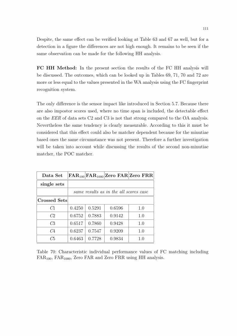
111

Despite, the same effect can be verified looking at Table 63 and 67 as well, but for adetection in a figure the differences are not high enough. It remains to be seen if thesame observation can be made for the following HH analysis.

FC HH Method: In the present section the results of the FC HH analysis willbe discussed. The outcomes, which can be looked up in Tables 69, 71, 70 and 72 aremore or less equal to the values presented in the WA analysis using the FC fingerprintrecognition system.

The only difference is the sensor impact like introduced in Section 5.7. Because thereare also impostor scores used, where no time span is included, the detectable effecton the EER of data sets C2 and C3 is not that strong compared to the OA analysis.Nevertheless the same tendency is clearly measurable. According to this it must beconsidered that this effect could also be matcher dependent because for the minutiaebased ones the same circumstance was not present. Therefore a further investigationwill be taken into account while discussing the results of the second non-minutiaematcher, the POC matcher.


single sets


Crossed Sets

C1 0.4250 0.5291 0.6596 1.0

C2 0.6752 0.7883 0.9142 1.0

C3 0.6517 0.7860 0.9428 1.0

C4 0.6237 0.7547 0.9209 1.0

C5 0.6463 0.7728 0.9834 1.0

Table 70: Characteristic individual performance values of FC matching includingFAR100, FAR1000, Zero FAR and Zero FRR using HH analysis.

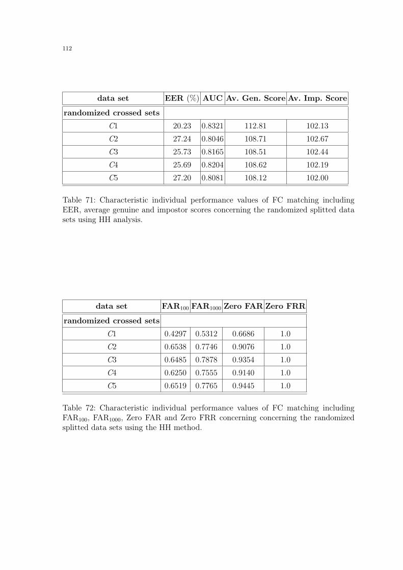
112



C1 20.23 0.8321 112.81 102.13

C2 27.24 0.8046 108.71 102.67

C3 25.73 0.8165 108.51 102.44

C4 25.69 0.8204 108.62 102.19

C5 27.20 0.8081 108.12 102.00

Table 71: Characteristic individual performance values of FC matching includingEER, average genuine and impostor scores concerning the randomized splitted datasets using HH analysis.



C1 0.4297 0.5312 0.6686 1.0

C2 0.6538 0.7746 0.9076 1.0

C3 0.6485 0.7878 0.9354 1.0

C4 0.6250 0.7555 0.9140 1.0

C5 0.6519 0.7765 0.9445 1.0

Table 72: Characteristic individual performance values of FC matching includingFAR100, FAR1000, Zero FAR and Zero FRR concerning concerning the randomizedsplitted data sets using the HH method.

113

As mentioned earlier this aspect is the most interesting one of the HH analysis forthe FC results. All the other characteristic performance values seem to be equal tothe WA and OA case. This leads to the assumption that ageing is not influencingthe performance of the fingerprint matching regarding the different types of impostorscores. For the used fingerprint recognition system the impostor scores are alwaysmore or less stable for each matcher and distinctively lower compared to the genuineones so far. So once more it seems that neither the randomized score selection processnor the impostor score split has an impact on the overall observed behavior of the usedfingerprint recognition system. The genuine score shift to the left caused by eitherthe imprints’ quality or fingerprint ageing can be verified for the first non-minutiaebased approach regardless which analysis method is used.


Single Sets

A 25.39 0.8218 0.2366 0.1121

B1 11.67 0.9376 0.2951 0.1070

B2 8.00 0.9635 0.3107 0.1088

B3 10.90 0.9408 0.2987 0.1080

B4 6.87 0.9672 0.3473 0.1096

B5 10.04 0.9415 0.3059 0.1131

Crossed Sets

C1 37.75 0.6892 0.1802 0.1091

C2 27.58 0.7958 0.2069 0.1103

C3 26.12 0.8080 0.2105 0.1106

C4 24.62 0.8273 0.2257 0.1110

C5 25.63 0.8164 0.2148 0.1122

Table 73: Characteristic individual performance values of POC matching includingEER, AUC, Average Genuine Score and Average Impostor Score using WA analysis.

114

5.8 2. POC Experiments:

Completing the presentation of the performance experiment results, the outcomes ofthe second experiments concerning the second non minutiae based matcher, the POCmatcher, will be described. As described before the result presentation starts withthe AS results to get an overview impression for the performance of fingerprint recog-nition system. The most interesting observation is based on the difference betweenthe average genuine and impostor scores of FC and POC.


Single Sets

A 0.4428 0.5260 0.7698 1.0

B1 0.2005 0.3178 0.6959 1.0

B2 0.1494 0.2479 0.5739 1.0

B3 0.1933 0.2882 0.5326 1.0

B4 0.1137 0.1862 0.6408 1.0

B5 0.1979 0.3107 0.7275 1.0

Crossed Sets

C1 0.6942 0.7418 0.8900 1.0

C2 0.5241 0.6354 0.8502 1.0

C3 0.5026 0.6167 0.8487 1.0

C4 0.4675 0.5766 0.8765 1.0

C5 0.4935 0.6179 0.8975 1.0

Table 74: Characteristic individual performance values of POC matching includingFAR100, FAR1000, Zero FAR and Zero FRR using WA analysis.

Although both methods are non minutiae based it seems that the second recogni-tion system is delivering more distinct outcomes in terms of clear separable averagematching scores. Of course using EER and considering the crossed data sets FC per-forms better, but for the single data sets from 2013 POC is performing much better.The results for the AS interpretation are available in Tables 73 and 74. Basically anidentical overall performance of POC like described for NBIS, NEURO and FC is

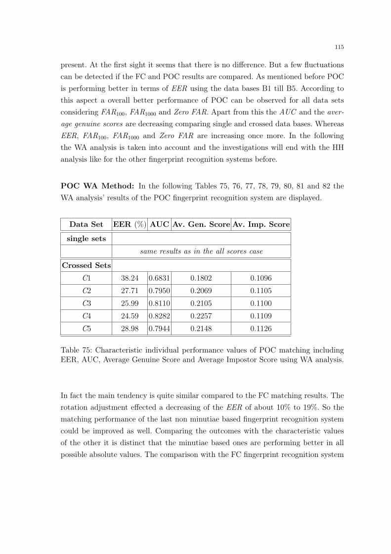
115

present. At the first sight it seems that there is no difference. But a few fluctuationscan be detected if the FC and POC results are compared. As mentioned before POCis performing better in terms of EER using the data bases B1 till B5. According tothis aspect a overall better performance of POC can be observed for all data setsconsidering FAR100, FAR1000 and Zero FAR. Apart from this the AUC and the aver-age genuine scores are decreasing comparing single and crossed data bases. WhereasEER, FAR100, FAR1000 and Zero FAR are increasing once more. In the followingthe WA analysis is taken into account and the investigations will end with the HHanalysis like for the other fingerprint recognition systems before.

POC WA Method: In the following Tables 75, 76, 77, 78, 79, 80, 81 and 82 theWA analysis’ results of the POC fingerprint recognition system are displayed.


single sets


Crossed Sets

C1 38.24 0.6831 0.1802 0.1096

C2 27.71 0.7950 0.2069 0.1105

C3 25.99 0.8110 0.2105 0.1100

C4 24.59 0.8282 0.2257 0.1109

C5 28.98 0.7944 0.2148 0.1126

Table 75: Characteristic individual performance values of POC matching includingEER, AUC, Average Genuine Score and Average Impostor Score using WA analysis.

In fact the main tendency is quite similar compared to the FC matching results. Therotation adjustment effected a decreasing of the EER of about 10% to 19%. So thematching performance of the last non minutiae based fingerprint recognition systemcould be improved as well. Comparing the outcomes with the characteristic valuesof the other it is distinct that the minutiae based ones are performing better in allpossible absolute values. The comparison with the FC fingerprint recognition system

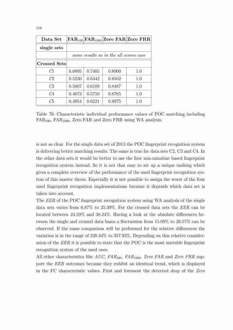
116


single sets


Crossed Sets

C1 0.6895 0.7405 0.8900 1.0

C2 0.5230 0.6342 0.8502 1.0

C3 0.5007 0.6109 0.8487 1.0

C4 0.4673 0.5750 0.8765 1.0

C5 0.4954 0.6221 0.8975 1.0

Table 76: Characteristic individual performance values of POC matching includingFAR100, FAR1000, Zero FAR and Zero FRR using WA analysis.

is not as clear. For the single data set of 2013 the POC fingerprint recognition systemis delivering better matching results. The same is true for data sets C2, C3 and C4. Inthe other data sets it would be better to use the first non-minutiae based fingerprintrecognition system instead. So it is not that easy to set up a unique ranking whichgives a complete overview of the performance of the used fingerprint recognition sys-tem of this master thesis. Especially it is not possible to assign the worst of the fourused fingerprint recognition implementations because it depends which data set istaken into account.The EER of the POC fingerprint recognition system using WA analysis of the singledata sets varies from 6.87% to 25.39%. For the crossed data sets the EER can belocated between 24.59% and 38.24%. Having a look at the absolute differences be-tween the single and crossed data bases a fluctuation from 15.09% to 26.57% can beobserved. If the same comparison will be performed for the relative differences thevariation is in the range of 238.44% to 357.93%. Depending on this relative consider-ation of the EER it is possible to state that the POC is the most unstable fingerprintrecognition system of the used ones.All other characteristics like AUC, FAR100, FAR1000, Zero FAR and Zero FRR sup-port the EER outcomes because they exhibit an identical trend, which is displayedin the FC characteristic values. First and foremost the detected drop of the Zero

117



C1 33.78 0.7375 0.1989 0.1083

C2 23.02 0.8391 0.2276 0.1100

C3 21.82 0.8487 0.2277 0.1092

C4 20.07 0.8709 0.2534 0.1100

C5 21.71 0.8523 0.2336 0.1122

Table 77: Characteristic individual performance values of POC matching includingEER, AUC, Average Genuine Score and Average Impostor Score concerning the split-ted data 2old3new using WA analysis.

FAR in data set C4 in the minutiae based fingerprint recognition systems can not beconfirmed in the POC. Both, the FC and POC results are supporting the assumptionthat this effect is an interesting observation caused by NBIS and NEURO. The sameis valid for the trend from FAR100 to Zero FAR. NBIS and NEURO are displaying adifferent one as for the non minutiae fingerprint recognition system.The performance of the WA analysis of the POC fingerprint recognition system isalso displayed in Figures 42 and 43 where two example ROC can be looked up. Thesetwo graphical representations are confirming once more that in the data set from 2009

there must be a lot of rotation and other positional variances within the fingerprintimages. Those fluctuations are the reason for the big differences between the perfor-mance of the single data sets from 2009 and 2013.

Based on the average genuine and impostor score distributions it is possible to detectquite the same effect as before looking at the other matching score distributions. Sothe genuine score distribution is also skewed to the left. There is a higher number oflow genuine scores in the crossed data set looking at Figures 45 and 44. But thereis also a difference. The number of impostor scores is also lower. In the followingChapter 6 it will be interesting to have a look at this effect.

In Figures 44 and 45 the shift in the genuine score distribution to the left can bedetected like in all other cases before. Additional to the genuine shift it can also

118



C1 0.6035 0.6681 0.8308 1.0

C2 0.4375 0.5637 0.8058 1.0

C3 0.4260 0.5433 0.8112 1.0

C4 0.3670 0.4750 0.8298 1.0

C5 0.4186 0.5568 0.8668 1.0

Table 78: Characteristic individual performance values of POC matching includingFAR100, FAR1000, Zero FAR and Zero FRR concerning the splitted data 2old3newusing WA analysis.

Fig. 42: ROC curves for single data sets A, B1 and crossed C1 using POC and WAanalysis.

be detected that there is a higher variability withing the total number of impostorscores. The reason for the impostor fluctuation probably is caused by the fingerprintrecognition system because it has not been observed in the other matching results.Therefore it will be necessary to have a more detailed look on this abnormality inOA and HH analysis of this fingerprint recognition system. Nevertheless the shift for

119



C1 41.83 0.6344 0.1653 0.1108

C2 31.22 0.7582 0.1903 0.1109

C3 29.32 0.7785 0.1967 0.1108

C4 27.97 0.7914 0.2035 0.1117

C5 28.82 0.7826 0.1997 0.1130

Table 79: Characteristic individual performance values of POC matching includingEER, AUC, Average Genuine Score and Average Impostor Score concerning the split-ted data 3old2new using WA analysis.

Fig. 43: ROC curves for single data sets A, B4 and crossed C4 using POC and WAanalysis.

the genuine scores and the more or less stability of the impostor scores for all casesleads to the confirmation of a first ageing effect.

120



C1 0.7577 0.7975 0.9157 1.0

C2 0.5924 0.6904 0.8702 1.0

C3 0.5630 0.6618 0.8583 1.0

C4 0.5444 0.6571 0.8422 1.0

C5 0.5571 0.6738 0.8746 1.0

Table 80: Characteristic individual performance values of POC matching includingFAR100, FAR1000, Zero FAR and Zero FRR concerning the splitted data 3old2newusing WA analysis.




Fig. 44: Genuine (colored red) and Impostor (colored yellow) score distribution of thePOC rotated A, B2 and C2 data set (x-axis denotes the matching scores and y-axisthe percentage scaled from 0 to 1) using WA analysis.

121



C1 38.28 0.6824 0.1803 0.1096

C2 27.75 0.7941 0.2065 0.1105

C3 25.98 0.8108 0.2106 0.1100

C4 24.50 0.8284 0.2257 0.1109

C5 25.81 0.8146 0.2148 0.1126

Table 81: Characteristic individual performance values of POC matching includingEER, average genuine and impostor scores concerning the randomized splitted datasets using WA analysis..




Fig. 45: Genuine (colored red) and Impostor (colored yellow) score distribution of thePOC rotated A, B3 and C3 data set (x-axis denotes the matching scores and y-axisthe percentage scaled from 0 to 1) using WA analysis.

122



C1 0.6895 0.7401 0.8730 1.0

C2 0.5239 0.6348 0.8382 1.0

C3 0.5009 0.6104 0.8330 1.0

C4 0.4668 0.5742 0.8372 1.0

C5 0.4951 0.6213 0.8751 1.0

Table 82: Characteristic individual performance values of POC matching includingFAR100, FAR1000, Zero FAR and Zero FRR concerning concerning the randomizedsplitted data sets using the WA method.

POC OA Method: In the present section the results for OA analysis of the POCfingerprint recognition system will be discussed. As for the other three fingerprintrecognition system there are mainly four tables which are representing the resultsof the performance analysis. Those Tables were 83, 85, 84 and 86. In Table 83 and84 the outcomes without size adaption for the crossed data sets are displayed. Theperformance characteristics for the randomized size adaption were presented in Table85 and 86.Examination of the results of the present POC based OA analysis leads to the conclu-sion that there is not a significant difference between this analysis and the previousWA one. Even having a closer look at the outcomes only reveals two slightly higherfluctuations. The first one can be located concerning the EER values. For data set C1in Table 83 the deviation is around 1.00% and for data set C5 around 3.50%. Bothvalues for the OA analysis are lower compared to the results of the without ageingimpostor (WA) analysis. It seems that the quite significant difference for the C5 database is caused by some random circumstance. Because for the randomly generatedsize adaption just the fluctuation of the C1 EER can be detected again looking atTable 81 and 85.The second variation is observable in the Zero FAR values which can be looked up inTable 84 and 86. As readable in Table 76 and 82 those Zero FAR outcomes are highercompared to the same results for the corresponding data sets in the OA analysis. It

123


single sets


Crossed Sets

C1 37.20 0.6952 0.1802 0.1087

C2 27.40 0.7965 0.2069 0.1102

C3 26.26 0.8050 0.2105 0.1111

C4 24.62 0.8282 0.2257 0.1112

C5 25.39 0.8185 0.2148 0.1119

Table 83: Characteristic individual performance values of POC matching includingEER, AUC, Average Genuine Score and Average Impostor Score using OA analysis.

(a) Genuine score distributionvs. impostor score distributionof the rotated data set A usingOA analysis.

(b) Genuine score distributionvs. impostor score distributionof the rotated data set B5 usingOA analysis.

(c) Genuine score distributionvs. impostor score distributionof the rotated data set C5 usingOA analysis.

Fig. 46: Genuine (colored red) and Impostor (colored yellow) score distribution of thePOC rotated A, B5 and C5 data set (x-axis denotes the matching scores and y-axisthe percentage scaled from 0 to 1) using OA analysis.

is interesting that the FAR100 and FAR1000 on the contrary seem to be more or lessstable.

124


single sets


Crossed Sets

C1 0.6980 0.7425 0.8214 1.0

C2 0.5255 0.6358 0.7926 1.0

C3 0.5039 0.6197 0.8414 1.0

C4 0.4676 0.5786 0.8437 1.0

C5 0.4917 0.6141 0.8640 1.0

Table 84: Characteristic individual performance values of POC matching includingFAR100, FAR1000, Zero FAR and Zero FRR using OA analysis.



C1 37.19 0.6948 0.1801 0.1087

C2 27.46 0.7959 0.2067 0.1102

C3 26.23 0.8051 0.2107 0.1111

C4 24.60 0.8261 0.2258 0.1112

C5 25.38 0.8181 0.2146 0.1119

Table 85: Characteristic individual performance values of POC matching includingEER, average genuine and impostor scores concerning the randomized splitted datasets using the OA method.

125

In Figure 46 it is also detectable that the genuine score distribution shift to the leftand the overall stability of the impostor scores occur like in all other cases before.Especially the very high number of low impostor scores like displayed in the middlegraphic of Figure 45 is also visible in the middle image of Figure 46 which wasintroduced before. Furthermore the clear trend that the genuine score distributionstend to adapt the impostor one is present in the right sub image of Figure 46.



C1 0.6982 0.7427 0.8194 1.0

C2 0.5258 0.6366 0.7841 1.0

C3 0.5031 0.6196 0.8123 1.0

C4 0.4678 0.5781 0.8249 1.0

C5 0.4920 0.6148 0.8279 1.0

Table 86: Characteristic individual performance values of POC matching includingFAR100, FAR1000, Zero FAR and Zero FRR concerning concerning the randomizedsplitted data sets using the OA method.

POC HH Method: In the last section of Chapter 5 the results for the outstandingHH analysis of the fourth fingerprint recognition system will be presented. Addition-ally the general information gained from this chapter will be discussed at the end ofthe present Section 5.8.

First of all the performance characteristics for the HH analysis of the POC fingerprintrecognition system can be looked up in Tables 87, 89, 88 and 90. The first impressionis that the outcomes are basically similar to the other two analysis methods presentedin the previous sections. This impression is true for many calculated values. Despite,it is also possible to gather an additional information. For the other fingerprint recog-nition systems discussed in this chapter the HH analysis was always a mixture of WAand OA. Of course that is probably the logical assumption, but for the POC this

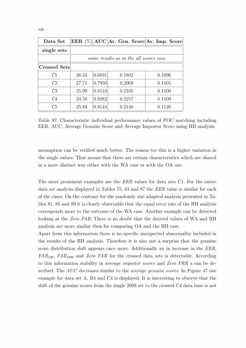
126


single sets


Crossed Sets

C1 38.24 0.6831 0.1802 0.1096

C2 27.71 0.7950 0.2069 0.1105

C3 25.99 0.8110 0.2105 0.1100

C4 24.58 0.8282 0.2257 0.1109

C5 25.84 0.8144 0.2148 0.1126

Table 87: Characteristic individual performance values of POC matching includingEER, AUC, Average Genuine Score and Average Impostor Score using HH analysis.

assumption can be verified much better. The reason tor this is a higher variation inthe single values. That means that there are certain characteristics which are sharedin a more distinct way either with the WA case or with the OA one.

The most prominent examples are the EER values for data sets C1. For the entiredata set analysis displayed in Tables 75, 83 and 87 the EER value is similar for eachof the cases. On the contrary for the randomly size adapted analysis presented in Ta-bles 81, 85 and 89 it is clearly observable that the equal error rate of the HH analysiscorresponds more to the outcome of the WA case. Another example can be detectedlooking at the Zero FAR. There is no doubt that the derived values of WA and HHanalysis are more similar then for comparing OA and the HH case.Apart from this information there is no specific unexpected abnormality included inthe results of the HH analysis. Therefore it is also not a surprise that the genuinescore distribution shift appears once more. Additionally an in increase in the EER,FAR100, FAR1000 and Zero FAR for the crossed data sets is detectable. Accordingto this information stability in average impostor scores and Zero FRR a can be de-scribed. The AUC decreases similar to the average genuine scores. In Figure 47 oneexample for data set A, B4 and C4 is displayed. It is interesting to observe that theshift of the genuine scores from the single 2009 set to the crossed C4 data base is not

127


single sets


Crossed Sets

C1 0.6895 0.7404 0.8845 1.0

C2 0.5228 0.6343 0.8461 1.0

C3 0.5010 0.6111 0.8424 1.0

C4 0.4673 0.5746 0.8574 1.0

C5 0.4953 0.6215 0.8905 1.0

Table 88: Characteristic individual performance values of POC matching includingFAR100, FAR1000, Zero FAR and Zero FRR using HH analysis.

very big. So a clear difference to the very distinct outcomes of for example NEUROcan be detected.

(a) Genuine score distributionvs. impostor score distributionof the rotated data set A usingHH analysis.

(b) Genuine score distributionvs. impostor score distributionof the rotated data set B4 usingHH analysis.

(c) Genuine score distributionvs. impostor score distributionof the rotated data set C4 usingHH analysis.

Fig. 47: Genuine (colored red) and Impostor (colored yellow) score distribution of thePOC rotated A, B4 and C4 data set (x-axis denotes the matching scores and y-axisthe percentage scaled from 0 to 1) using HH analysis.

128



C1 25.56 0.8161 0.2106 0.1091

C2 27.66 0.7945 0.2066 0.1103

C3 26.13 0.8077 0.2106 0.1106

C4 24.57 0.8271 0.2257 0.1110

C5 25.63 0.8160 0.2147 0.1122

Table 89: Characteristic individual performance values of POC matching includingEER, average genuine and impostor scores concerning the randomized splitted datasets using the HH method.

Fig. 48: ROC curves of data set A using results from all used fingerprint recognitionsystem types using HH analysis.

Based on the knowledge about each fingerprint recognition systems’ performance itis possible to summarize and compare the results. First there can be a comparison interms of the ROC curves. In Figures 48 and 49 this is displayed. In Figure 48 dataset 2009 is pictured. In the second Figure 49 the crossed data set C2 is depicted. For

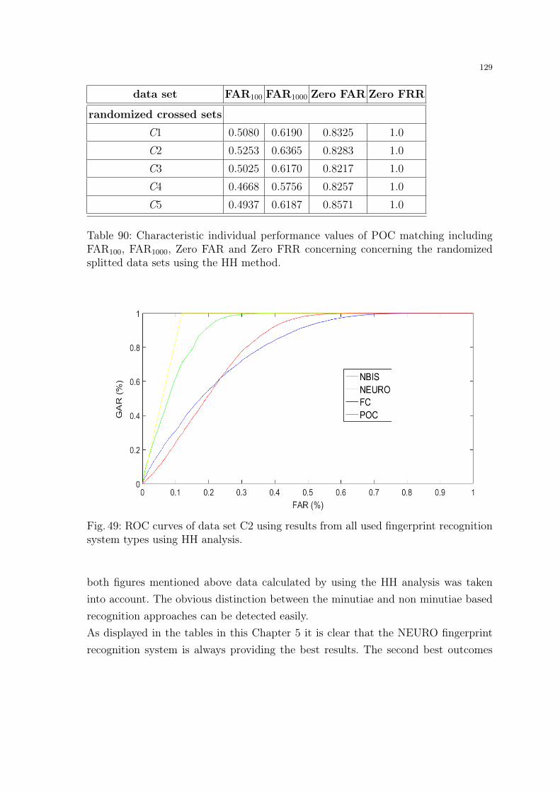
129



C1 0.5080 0.6190 0.8325 1.0

C2 0.5253 0.6365 0.8283 1.0

C3 0.5025 0.6170 0.8217 1.0

C4 0.4668 0.5756 0.8257 1.0

C5 0.4937 0.6187 0.8571 1.0

Table 90: Characteristic individual performance values of POC matching includingFAR100, FAR1000, Zero FAR and Zero FRR concerning concerning the randomizedsplitted data sets using the HH method.

Fig. 49: ROC curves of data set C2 using results from all used fingerprint recognitionsystem types using HH analysis.

both figures mentioned above data calculated by using the HH analysis was takeninto account. The obvious distinction between the minutiae and non minutiae basedrecognition approaches can be detected easily.As displayed in the tables in this Chapter 5 it is clear that the NEURO fingerprintrecognition system is always providing the best results. The second best outcomes

130

are provided by the NBIS fingerprint recognition system. Furthermore, the minutiaebased fingerprint recognition systems are performing better then the non minutiaeones. In Figure 49 it is displayed that sometimes the FC performance and sometimesthe POC performance is slightly worse compared with the other non-minutiae basedfingerprint recognition system in a limited area of the ROC. According to the infor-mation that two different data sets have been used to construct those visualizations adata set dependent variation is present as well. It remains an open question whetherthe used sensor types are responsible for this or probably the user behavior duringimprint acquisition. In general there is no doubt that the performance of both nonminutiae based fingerprint recognition system is not anything like as good as NEUROand NBIS. Judging from the fact that not only the overall performance is not thebest, it is also observable that the ageing effect is not that high as for the NEUROfingerprint recognition system. Especially for the FC recognition system the equaliza-tion trend of both score distributions is much lower compared to the remaining threemethods. The shift in the genuine score distribution to the left is much lower becauseof the anyway present high similarity of the matching scores. This circumstance canbe observed looking at Figures 35 and 39. Those two figures are just representatives.The situation is always identical for each used data base. The ageing effect, the gen-uine score shift to the left, can be detected in each data set and for every fingerprintrecognition system. The only variance can be observed in the intensity. For example,comparing both minutiae based fingerprint recognition systems a distinct differenceis available. In Figures 27 and 34 this is clearly recognizable. For this purpose as afinal statement for this chapter it is realistic to state the following conclusion: ’Age-ing effects in terms of shifted score distributions can be detected for each fingerprintrecognition system and sensor type independently how good the matching accuracylooks like.’

131

6 Doddington’s Zoo and Menagerie Analysis

Before talking about ageing effects in detail it is necessary to focus on the topicconcerning the fingerprint image quality. As discussed in Sections 4.4 and 5.6 thequality respectively the variety during the acquisition process of the imprints areimportant and deliver a huge impact in the recognition performance of used matchertechniques. Independently, there are a lot of different effects that can occur andeventually affect matching results. In Section 4 those that can be detected in theused data sets are represented. There are a lot of reasons why such degradationsemerge. Aside from the fact that there are medical reasons like arthritis or injurieslike cuts reducing the imprints’ quality also natural human ageing must be takeninto account. So the loss of collagen impacts the texture of the skin and effects forexample dry skin [24].In the following Section 6.1 there will be a short discussion how to characterizethe different properties of people within a recognition system. There will be twodifferent parts. On the one hand a pure statistical analysis using two hypothesistesting methods are applied to verify that those types of characterizations exit. Onthe other hand a distinct search for so called animal behavior using a combination ofempirical and statistical methods is performed. The different methods are based on[12], [31] and [40].

6.1 Doddington Zoo

The idea of characterizing differences in recognition systems based on the individu-ality of the user was first presented in 1998 by George Doddington et al. [12]. Theyperformed a speaker analysis searching for different types of speaker behavior withinautomatic recognition systems. It was possible to describe four different types socalled ’animals’. Each of them shows a specific behavior and users can be labeled toa specific animal type, due to the fact that the match score distribution will exhibithigh as well low genuine and impostor values. According to the similarity scores it ispossible to detail the basic animal types as follows.

– Sheep: Those types are the so called default users. They are dominant withinthe population and perform well on recognition systems. Based on the genuinescores they receive high scores while matching against themselves and low values

132

if compared to other individuals. Therefore they tend to imply a low FRR becausetheir features are separating them well from all the other inputs.

– Goats: As opposed to the first class, the second type based on genuine scoresare those who are awkward to recognize. Because they are gathering low genuinescores they are affecting false rejections.

– Lambs: The interesting characteristic of them is the feature set that produces anoverlap with other individuals within the data base. It is quite easy to imitatethem and effecting an increase of the FAR. ’Lambs, on average, tend to producehigh match scores when being matched against by another user [40].’

– Wolves: Wolves are those users who are gaining high match scores when matchedagainst other individuals in the data set. So they can be found while looking at theimpostor scores again and are very similar to lambs. They can cause false acceptsand according to [12] finding wolves represents a possible system weakness. InSection 6.2 there will be a short discussion about the similarity between lambsand wolves.

Beyond the before mentioned basic types of user behavior there are some other ani-mals that can be found as well. In the present work they will not be covered but forthe sake of completeness they will be introduced shortly. They have been introducedby Neil Yager and Ted Dunstone in 2010 [40]. As opposed to sheep, goats, lambsand wolves they are not based only on the genuine and impostor scores. Worms,chameleons, phantoms, and doves are defined using the relationship between thematching values. So, for example, doves are the best user type that can be foundwithin any data base. They retrieve high scores when matched against themselvesand also low values when matched against others. Whereas worms are causing thebiggest problems that can occur. They are gathering low genuine as well high impos-tor scores increasing the recognition system errors.

6.2 Menagerie Analysis - Pre-Information and Assumptions

Performing the menagerie calculation and proving the existence of sheep, goats, lambsand wolves a set of different methods will be applied. Due to the fact that sheepare the so called default user there will not be a specific investigation on those moretheoretical types. The second important clarification is about lambs and wolves. Since

133

during the matching the symmetric calculations have not been executed to avoidcorrelation it is not possible to distinguish between those two types. In the lambscase the user of interest is already contained in the gallery. For the wolves calculationthe person of interest is the so called probe user. For this purpose both definitionsare equivalent for the used performance experiments. In the following lambs andwolves will be treated as one combined class. Actually the menagerie analysis will befocused on two classes. On the one hand the goat class and on the other hand thelambs/wolves class.Furthermore it is necessary to set up a few assumptions which will be consideredin the menagerie investigations. According to the performance analysis, displayed inChapter 5, the degradation of genuine scores and stability of impostor scores leadsto the following two hypotheses. The fluctuation’s amount among the number ofdifferent users signed as a goat in the crossed data sets will be quite high. Based onthe genuine scores degradation there won’t be a lot of volunteers who can be markedas goat-like in data sets from 2009, 2013 and in the crossed ones. As opposed to thisa high amount of stability in terms of different lamb-/wolf-like users is assumed dueto the stability of the impostor scores. Apart from those two main hypothesis it isalso interesting to have a look on the comparison between minutiae based and non-minutiae based fingerprint recognition systems. Probably there are no differencesbased on the menagerie analysis detectable. Furthermore, the impact of the usedanalysis methods (mean, variance, mean2 and minimum/maximum) will be a crucialone too. Those methods will be introduced in the following Section 6.3.

6.3 Menagerie Analysis - Experiments and Results

In the following subsection there will be a discussion on the analysis of the performedexperiments concerning the different animal types. At first, an existence analysis wasperformed to verify if they are available. After this calculation a specific search forsingle users characterized as an animal type was executed.

Existence Analysis In [12] there are three methods used to perform a statisticalexistence analysis of goats, lambs and wolves. F-Test, Kruskal-Wallis Test and DurbinTest have been chosen. In the present thesis two of them have been used as well. Onthe one hand the F-Test and on the other the Kruskal-Wallis Test are executed. In

134

both cases the null hypothesis was said to be that there are no such special char-acterizations in the data sets. That means that it is not possible to find differencesbetween the individual score distributions. For both tests a significance level of 0.01was taken.

F-Test: Each statistical test respectively the test statistic that follows the F-distributioncan be assigned to be an F-Test. In the present work a classical one-way analysis ofvariance (ANOVA) test has been used in the same way as described in [12]. As men-tioned in [40] there is a slight problem. Due to the fact that the well known standardF-Test expects a normal distributed data set it is clear that this cannot be guar-anteed. Looking at the genuine and impostor distributions pictured in Section 5 itseems that the scores approximate in some way a normal distribution. Therefore thehypothesis test has been performed on the given matching data. Regrading the be-forehand null hypothesis and significance level on each data set there was the sameresult no matter if looking for goats or for lambs/wolves. The null hypothesis mustbe rejected for all data bases and matching results. Even when performing the sametesting on another significance level of 0.05.

Kruskal-Wallis Test: The Kruskal-Wallis Test or also called H-Test is a non-parametricone-way analysis of variance by ranks test that does not need a normal distributeddata set. Therefore, this test is well suited for the given data situation. The big dif-ference to the before used F-Test is the replacement of the matching scores. Thisimplies that the matching values are replaced by ranks. There is also a limitation ofthe test as well, it is mandatory to have at least five samples from each finger. Apartfrom this the null hypothesis and the significance level remain same as before. Forthe goats and lambs/wolves calculations that have been performed according to [12],the null hypothesis must be rejected once again. So at a significance level of 0.01 thealternative hypothesis that there are goats, lambs and wolves within the data setscould be accepted.

User Analysis Theory The user analysis refers to the effective search for usersthat can be characterized as a certain animal type. Regarding to the previous partof the thesis the existence of goats and lambs/wolves is confirmed. In the followingparagraph four different methods will be used to identify these individuals:

135

– mean scores method: The first method is based on the mean scores like presentedin [12]. The idea is to describe the behavior of each user by the expected value oftheir associated match score distribution. So the mean of all match scores belong-ing to a person is calculated. After performing this step for all people within thedata set the list of all mean scores is sorted. Based on the paper of Doddingtonfrom 1998 the lowest and highest 2.5% of those values are assigned to represent ananimal behavior. The related user is signed to be a goat or lamb/wolf. Concerningthe two different types of characteristics there must be a distinction between thecalculation details. In the goat case simply all matching scores are used. Look-ing at the lamb/wolf case there is a small difference due to the calculated scores.According to the methodology the impostor scores have been derived with, thereare 5 or 10 sets of independent values. For each set and for each user the maxi-mum impostor score is evaluated. That means that for each individual the meanimpostor score is derived out of 5 or 10 maximum values before sorting them andcalculating the goat-like or lamb-/wolf-like users.

– variance scores method: This method is also presented in [12]. Basically the samecalculation is performed as mentioned before. The only difference is the use ofvariance instead of the expected value.

– mean2 scores method: The third alternative is based on [31]. That means thatoriginally after deriving the mean values as before and sorting them, the userswhose mean values is lower than the 30-th percentile are labeled as goats. In thelamb/wolf case those are assigned to be a lamb/wolf whose mean score is belowthe 10-th percentile. During the first experiments it becomes apparent that thechosen percentiles are much too high compared to the other values. Therefore theyhave been adapted. So in both cases the 5-th percentile will be taken into account.

– minimum/maximum scores method: This method is using an empirical idea. Forthe goats calculation the lowest value of each user distribution is chosen. Thosegenuine score values are sorted afterwards and the user who are assigned to thelowest 5-th percentile are labeled as goat. The calculation in the lamb/wolf caseis quite similar except for the fact that not the lowest impostor scores of the userdistributions have been taken, but the maximum values.

Based on those methodologies there are some weaknesses that must be discussed aswell. The problem concerning the last menagerie analysis method is the quite high

136

sensitivity to outliers. Especially looking at the genuine and impostor scores of theNEURO matching it is clear that those can cause some problems in the further analy-sis. The majority or to be more precise almost all matching scores using the NEUROimplementation are 0 across all data sets. For sure that is not only a problem for theminimum/maximum method.The mean, mean2 and variance (var) method are robust to those outliers. That is thebiggest advantage. But apart form this there is also a slight weakness to be coveredlater on. The disadvantage is the not confirmed relationship between the mean scoresand the contribution to possible system errors. According to [40] this participationmust be considered in a separate experimental setting. The results of this experimentswill be presented at the end of the chapter in Section 6.5. But before the results ofthe performed investigations will be presented.

6.4 User-defined Menagerie Analysis Results

In this Section of the master thesis the detailed menagerie user analysis results will bepresented. At first there will be a discussion about the goat-like behavior of differentusers within the data sets. In the second part the analysis results for the lambs/wolvesexperiments are taken into account. The user-defined menagerie analysis can be sum-marized by means of plotting the user’s average genuine scores against the user’saverage impostor scores. So to get a general overview, Figure 50 can be used to getan impression of where the different animal types can be found. The plots displayedin Figures 51, 52, 53 and 54 visualize the existence of goats and lamb/wolves, but alsothe other ’animal’-like characteristics described before. To be more precise in the firstfigure, Figure 51, the different animal types and their position according to Figure50 are marked. The signed goat-like (red colour) and lamb/wolf-like (green colour)volunteers have been calculated using the mean method. The dark blue colored usersare displaying no special behavior and those who are signed in cyan represent thesheep case. Those sheep-like volunteers have been selected using a rectangle shapedarea around the center of the mean scores according to their assumed location.In the before mentioned figures the presence of goats is detectable looking at the lowuser’s genuine scores indicated at the x-axis. The higher values shown on the y-axisare representing the lamb/wolf-like users. It is clearly observable that all animal types

137

Fig. 50: General overview of the position of the different animal types according totheir definition introduced in subsection 6.1.

can be detected in each data set and across all used recognition systems looking forexample at the marked entries in Figure 51. But those four figures are just represent-ing the situation using the mean menagerie analysis method. Using the user’s averagevariance scores the distinction between the animal types is not always so clear, butnevertheless the existence of goats and lambs/wolves can be verified once again. Thissituation is displayed in Figure 55.Basically, the most important information about the menagerie analysis is the factthat not single imprints are labeled as an animal type rather users are labeled. Eachdata sets contains 196 users as introduced in Section 4. Due to the described menagerieanalyzing methods always a fixed number of volunteers will be labeled as goats orlambs/wolves. The reason for this is that depending on the matching results for ex-ample the users with a mean matching score value less than the 5 percentile scorevalue are signed. So the higher number of imprints in the crossed data sets is not di-rectly influencing this analysis. There is just a small impact. For example think aboutthe mean score calculation used in the mean method. The higher number of imprintsguarantee a higher number of matching values. For this purpose, within the meanscore calculation, more values are taken into account but this is the only differencebetween the crossed and the single data sets. For each user the mean score value isused to perform the animal type labeling.

138

Fig. 51: User’s average mean genuine scores (x-axis) and user’s average mean impostorscores (y-axis) using NBIS and data A in the first graphic, B4 in the second one andC4 in the last one.

139

Fig. 52: User’s average mean genuine scores (x-axis) and user’s average mean impostorscores (y-axis) using NEURO and data set A in the first graphic, B3 in the secondone and C3 in the last one.

140

Fig. 53: User’s average mean genuine scores (x-axis) and user’s average mean impostorscores (y-axis) using FC and data set A in the first graphic, B2 in the second one andC2 in the last one.

141

Fig. 54: User’s average mean genuine scores (x-axis) and user’s average mean impostorscores (y-axis) using POC and data set A in the first graphic, B1 in the second oneand C1 in the last one.

142

Fig. 55: User’s average variance genuine scores (x-axis) and user’s average varianceimpostor scores (y-axis) using NBIS and data set A in the first graphic, B2 in thesecond one and C2 in the last one.

143

Before talking about goats there is a short part about sheep. For sure there was notan experimental setting to verify sheep-like users, but nevertheless during the goatsanalysis the question, which users are never signed to be goat-like, occurred. So thenon goat-like term ’never occur’ must be explained. In this context it means that allthose were signed to be non goat-like if they are never included in the goats analysisno matter what data base is looked at. So in Table 91 the number of those users islisted.Due to that fact there are always 11 users labeled for the mean and variance methodand 10 for the mean2 method. The minimum/maximum method is the sole excep-tion. There is a specific reason for this effect. After looking at the for example 5

percentile score value, not only the lower score values are taken into account. Thereis also a comparison to those score values that are next in the value ordering. Allfollowing values that are of the same size as the 5 percentile score value, are alsolabeled as a specific animal type. This is done because the score values are the samebut due to the ordering they would not be taken into account, but in fact they haveto. The ordering is performed according to the users ID and it would not be correctto ignore them because they have the same low score value as the threshold percentile.

Goats Analysis: Due to the definition of sheep, the so called ’default user type’,it is clear that the users displayed in Table 91 could be signed as sheep. But theywill be signed as not goat-like and not as sheep-like because no explicit sheep exper-iments have been performed. For each matching method there are some users thatare always included in the non goat-like list. Those volunteers could be determinedwith no respect to a specific data set/sensor type.

Looking at Table 91 it is necessary to remember that the maximum number of enrolledusers is 196. According to this, it is important to look at the amount of non goat-likeusers in more detail. That means, that the number of non goat-like users is varyingbetween 73.98% in the mean2 method for NBIS and POC matcher and 13.78% in theminimum method for the NEUROmatcher. Especially remarkable is the circumstancethat the three numbers that are far below the 50% line are all for the minimumanalysis method. Apart from this there is no other analysis method that seems to bevery sensitive to the matching scores. But as discussed in Section 6.3 it was very likely

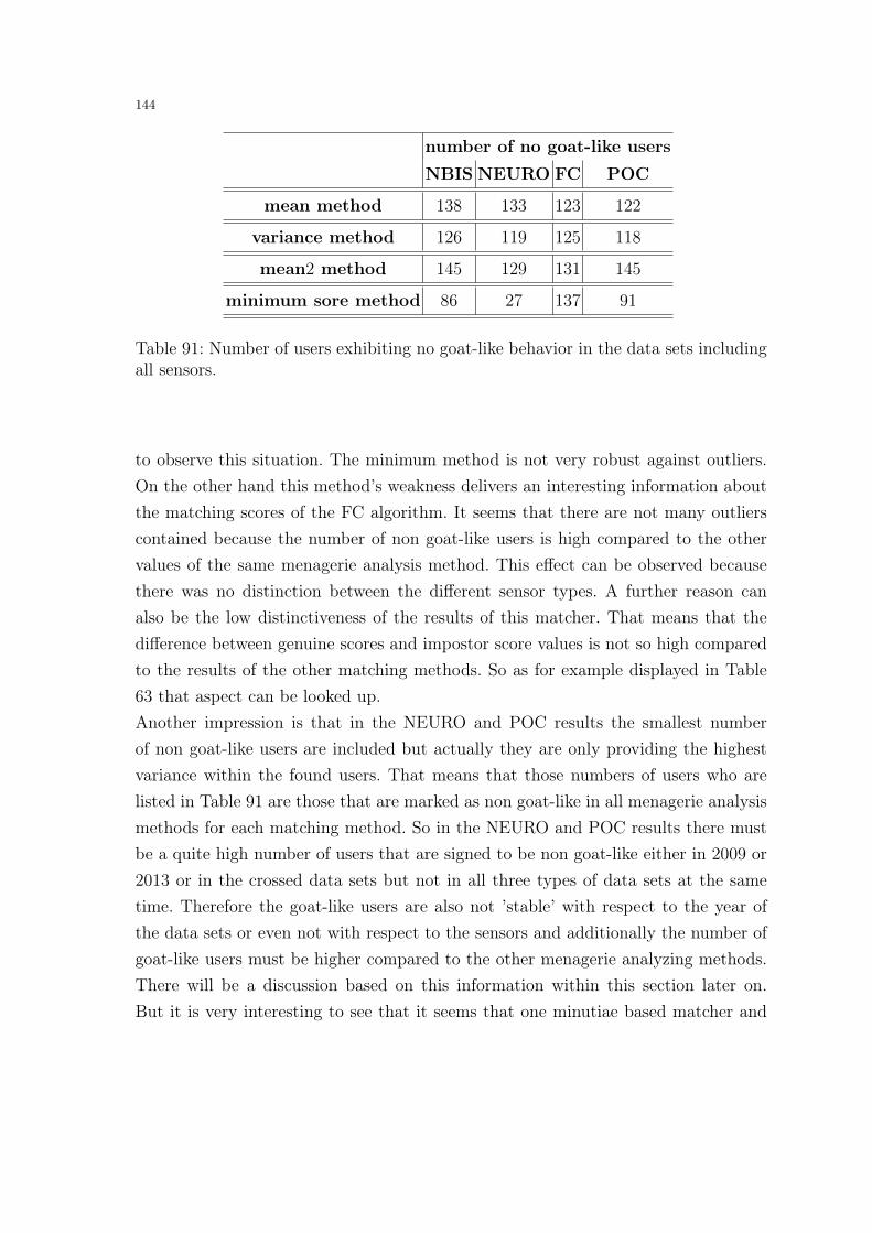
144

number of no goat-like users

NBIS NEURO FC POC

mean method 138 133 123 122

variance method 126 119 125 118

mean2 method 145 129 131 145

minimum sore method 86 27 137 91

Table 91: Number of users exhibiting no goat-like behavior in the data sets includingall sensors.

to observe this situation. The minimum method is not very robust against outliers.On the other hand this method’s weakness delivers an interesting information aboutthe matching scores of the FC algorithm. It seems that there are not many outlierscontained because the number of non goat-like users is high compared to the othervalues of the same menagerie analysis method. This effect can be observed becausethere was no distinction between the different sensor types. A further reason canalso be the low distinctiveness of the results of this matcher. That means that thedifference between genuine scores and impostor score values is not so high comparedto the results of the other matching methods. So as for example displayed in Table63 that aspect can be looked up.Another impression is that in the NEURO and POC results the smallest numberof non goat-like users are included but actually they are only providing the highestvariance within the found users. That means that those numbers of users who arelisted in Table 91 are those that are marked as non goat-like in all menagerie analysismethods for each matching method. So in the NEURO and POC results there mustbe a quite high number of users that are signed to be non goat-like either in 2009 or2013 or in the crossed data sets but not in all three types of data sets at the sametime. Therefore the goat-like users are also not ’stable’ with respect to the year ofthe data sets or even not with respect to the sensors and additionally the number ofgoat-like users must be higher compared to the other menagerie analyzing methods.There will be a discussion based on this information within this section later on.But it is very interesting to see that it seems that one minutiae based matcher and

145

one non-minutiae based matcher are delivering ’stable’ results in terms of goat-likemenagerie analysis.

Based on the non goat-like experiments the more interesting task is the search forusers characterized as animal type ’goat’. In the following Tables 92, 93, 94 and 95the results for the goat experiments are displayed. For each matcher type and dataset the same experiment was performed, gathering the results as depicted in thebefore mentioned four tables. For each menagerie analyzing method the investigationwas performed year dependent. So in the first step for each data set the data basedependent goat-like volunteers have been marked. To get an overall description of allthose special users which occur, the single results are combined. So the volunteerseffecting a goat-like behavior are clustered to three centers. In the Tables 92 till95 the data set from 2009 will be called ’old’. The data sets from 2013 are called’new’ altogether and finally the crossed data sets from 209 and 2013 will be named’crossed’. Looking at the results the first important fact is the poor performance ofthe minimum method. While there is a long list for the NBIS results, there wouldhave been too many users marked as a goat in the NEURO and POC results. Thiscircumstance proves the results from the non goat results for those two matchers. Sothere are a lot of users signed as goat-like in the NEURO and POC results. Apartfrom this information it is clearly observable that there are differences between thegoat-like users. That means that there are a lot of ’goats’ which are occurring just inthe ’old’ data set or in one of the ’crossed’ one for example. So in fact it is possibleto differentiate between five classes of occurrence:

– Class 1: Those volunteers are labeled as goat only once in 2009, 2013 or in thecrossed data sets. Looking at the NBIS results for the mean menagerie analysismethod user 154 belongs to this class.

– Class 2: There are some users which are signed to have a goat-like behavior inall of the different years, like volunteer 100 as displayed using mean method andthe corresponding NBIS results.

– Class 3: The volunteers assigned to this class are labeled in 2009 and 2013. Sousing the same analysis set as in the classes before, user 21 is detected in 2009

and in the T2 data set from 2013.

146

Data Set User ID

matcher NBIS

mean method

old 21, 25, 47, 56, 64, 86, 98, 100, 131, 134, 154

new 1, 2, 3, 4, 6, 12, 13, 14, 20, 21, 25, 27, 30, 33, 36, 37, 38, 44, 45,50, 54, 55, 62, 64, 69, 74, 78, 82, 85, 88, 90, 98, 100, 103, 129, 136

crossed 3, 4, 5, 6, 27, 29, 32, 47, 52, 53, 56, 80, 86, 87, 91, 100,112, 119, 123, 124, 129, 131, 134, 159, 162, 170, 187

variance method

old 9, 10, 47, 49, 56, 78, 100, 129, 134, 142, 158

new 1, 2, 3, 4, 6, 7, 8, 14, 18, 29, 30, 35, 36, 41, 48, 51, 52, 55,64, 66, 74, 77, 78, 79, 82, 86, 90, 92, 96, 103,

104, 114, 121, 129, 130, 132, 139, 148, 156, 157, 185

crossed 4, 5, 8, 10, 16, 27, 29, 35, 46, 47, 48, 56,61, 62, 64, 76, 78, 80, 86, 92, 98, 100, 101, 113, 123,

124, 130, 133, 134, 137, 154, 163, 168, 178, 187

mean2 method

old 5, 21, 25, 129, 130, 131, 134, 154, 159, 163

new 6, 11, 12, 13, 14, 16, 20, 25, 27, 33, 36, 38, 41, 44, 48, 51, 63,64, 69, 70, 74, 78, 82, 83, 89, 103, 129, 136, 163, 164, 185

crossed 5, 16, 21, 22, 25, 26, 27, 72, 80, 119, 129, 131, 132,134, 154, 158, 159, 160, 161, 162, 163, 170, 178, 187

minimum sore method

old 9, 10, 11, 32, 36, 55, 56, 69, 71, 75, 86, 87, 112

new 1, 2, 3, 4, 11, 19, 21, 29, 30, 37, 40, 45, 46, 49, 50, 52, 54,55, 57, 62, 65, 66, 69, 72, 76, 81, 85, 88, 89, 90, 91, 98, 100,106, 109, 110, 117, 118, 121, 122, 125, 126, 127, 128, 134,

140, 145, 147, 148, 153, 156, 158, 173, 182, 183

crossed 1, 2, 3, 4, 9, 10, 11, 12, 15, 17, 18, 19, 23, 29, 30, 31, 32, 34, 36,38, 39, 44, 47, 48, 50, 52, 53, 54, 55, 56, 57, 58, 60, 64, 68, 71, 74, 75,77, 78, 83, 84, 86, 87, 88, 91, 92, 93, 97, 98, 100, 105, 107, 108, 112,115, 119, 120, 125, 126, 127, 128, 129, 136, 137, 138, 139, 145, 146,

148, 154, 155, 156, 157, 174, 175, 180, 185, 195

Table 92: User exhibiting a goat-like behavior in the NBIS data sets including allsensors.

147

Data Set User ID

matcher NEURO

mean method

old 6, 9, 10, 25, 26, 47, 56, 64, 122, 124, 176

new 1, 2, 3, 4, 10, 18, 19, 20, 25, 38, 39, 53, 54, 55, 57, 60, 66, 76, 78,86, 92, 98, 117, 119, 129, 133, 153, 156,

163, 166, 169, 171, 177, 179, 180, 185, 192, 194

crossed 1, 3, 4, 6, 21, 24, 29, 32, 47, 53, 56, 56, 64, 74, 80, 88, 110,122, 123, 124, 131, 132, 140, 153, 154, 162, 169, 170, 176, 187

variance method

old 10, 14, 44, 47, 58, 66, 88, 113, 122, 124, 129

new 1, 2, 3, 4, 6, 12, 18, 19, 20, 30, 35, 38, 51, 52, 54, 55, 56, 59,66, 71, 74, 76, 78, 88, 91, 92, 108, 115, 120, 121,

122, 125, 126, 146, 150, 153, 157, 163, 175, 176, 188, 192

crossed 9, 10, 29, 30, 32, 35, 45, 46, 47, 48, 51, 53,55, 56, 58, 60, 61, 69, 74, 79, 84, 86, 87, 97, 98,

100, 101, 110, 122, 123, 124, 136, 146, 154, 156, 160, 176, 178, 179, 180

mean2 method

old 5, 6, 25, 26, 64, 135, 146, 165, 176, 193

new 10, 12, 23, 25, 27, 34, 38, 39, 47, 48, 53, 54, 58, 60, 61, 70,78, 86, 92, 97, 117, 119, 129, 133, 138, 140, 156, 163,

164, 166, 169, 171, 177, 179, 180, 185, 186, 187

crossed 6, 21, 24, 25, 27, 63, 64, 72, 79, 80, 84, 88, 110,118, 129, 131,132, 139, 140, 154, 158, 159, 161, 162, 169, 170, 171, 172, 176, 187

minimum sore method

old 9, 10, 11, 15, 29, 32, 47, 49, 55, 56, 58, 69, 71, 74, 75, 77,78, 87, 112, 123, 124, 127, 128, 128, 140, 153, 155, 156, 157, 168, 192

new too many entries due to outlierscrossed too many entries due to outliers

Table 93: User exhibiting a goat-like behavior in the NEURO data sets including allsensors.

148

Data Set User ID

matcher FC

mean method

old 107, 109, 115, 124, 151, 153, 154, 156, 163, 174, 196

new 1, 6, 38, 44, 65, 66, 67, 68, 70, 72, 76, 86, 125, 126, 128, 129,135, 137, 138, 144, 149, 151, 152, 153, 154, 155, 157,

170, 173, 175, 179, 181, 182, 183, 185, 187, 188, 190, 192, 194, 195

crossed 4, 5, 6, 11, 15, 16, 17, 18, 20, 21, 24, 26, 27, 32, 41, 44, 55, 56, 62,65, 67, 68, 88, 111, 131, 136, 137, 139, 140, 159, 163, 183, 190, 191

variance method

old 26, 27, 75, 79, 113, 114, 167, 171, 172, 183, 193

new 3, 15, 17, 25, 27, 30, 32, 34, 41, 44, 48, 50, 52, 56, 59, 72, 74,75, 85, 102, 107, 113, 114, 115, 117, 119, 120, 122, 127,

128, 133, 128, 133, 138, 139, 145, 153, 156, 159, 160, 168, 181, 195

crossed 2, 6, 14, 15, 16, 21, 24, 26, 27, 32, 39, 44, 47, 48, 56, 59,60, 61, 62, 68, 72, 75, 79, 102, 107, 108, 111, 115, 119, 121,

124, 125, 134, 136, 139, 153, 159, 171, 172, 179, 183, 195, 196

mean2 method

old 107, 109, 111, 115, 120, 121, 124, 136, 139, 151

new 1, 3, 16, 38, 46, 69, 70, 72, 86, 129, 131, 137, 138, 142, 144, 149, 151,161, 168, 173, 175, 179, 180, 181, 183, 184, 185, 187,190, 193, 195

crossed 5, 6, 7, 16, 21, 22, 24, 25, 26, 27, 28, 37, 49,50, 57, 60,64, 76, 79, 82, 83, 84, 86, 99, 164, 169

minimum sore method

old 55, 56, 67, 75, 108, 158, 167, 175, 182, 193

new 1, 2, 3, 4, 7, 18, 22, 23, 37, 50, 52, 58, 65, 66, 67, 68, 91, 99, 112, 117,119, 122, 125, 126, 127, 128, 134, 153, 156, 157, 159, 160, 168, 173

crossed 17, 35, 48, 50, 55, 56, 61, 62, 66, 67, 68, 70, 75, 93, 102, 108, 125,126, 154, 158, 161, 163, 164, 167, 174, 179, 182, 190, 193, 195

Table 94: User exhibiting a goat-like behavior in the FC data sets including all sensors.

149

Data Set User ID

matcher POC

mean method

old 16, 17, 22, 25, 27, 108, 172, 180, 190, 191, 192

new 6, 8, 10, 11, 12, 13, 14, 23, 25, 27, 36, 38, 44, 74, 78, 82,103, 104, 108, 109, 110, 113, 117, 118, 119, 125, 127, 128, 131,140, 153, 155, 156, 158, 174, 176, 178, 182, 183, 184, 190, 194

crossed 1, 3, 6, 7, 16, 18, 19, 20, 21, 24, 25, 26, 27, 37, 50,64, 70, 83, 84, 99, 105, 106, 108, 112, 125, 150, 153,154, 155, 164, 175, 180, 182, 190, 192, 195, 196

variance method

old 35, 48, 71, 77, 100, 120, 121, 151, 152, 156, 169

new 3, 4, 17, 18, 21, 29, 30, 31, 43, 46, 49, 53, 55, 56, 57, 58, 63, 66,79, 94, 98, 99, 114, 115, 116, 119, 120, 124, 133, 138, 140,

148, 156, 157, 162, 164, 166, 169, 170, 171, 176, 179, 185, 186, 191

crossed 13, 14, 19, 27, 33, 35, 36, 44, 48, 53, 55, 66, 70, 71, 74, 75,77, 80, 94, 100, 113, 114, 116, 118, 121, 122, 135, 139, 140, 146,

153, 154, 164, 169, 171, 172, 174, 177, 187, 188, 189

mean2 method

old 16, 17, 19, 22, 25, 27, 30, 50, 54, 80

new 5, 6, 8, 9, 10, 11, 12, 13, 14, 21, 23, 24, 25, 27, 33, 34, 35,36, 38, 39, 42, 43, 44, 52, 60, 62, 64, 74,75, 78, 82, 83, 84

crossed 5, 6, 7, 8, 11, 12, 15, 16, 21, 22, 23, 24, 25,26, 27, 28,37, 61, 64, 76, 80, 89, 99

minimum sore method

old too many entries due to outliersnew too many entries due to outliers

crossed too many entries due to outliers

Table 95: User exhibiting a goat-like behavior in the POC data sets including allsensors.

150

– Class 4: This class is displaying those users assigned to be a goat in 2009 and thecrossed data sets. Looking at the menagerie results using the uru4500 data setsvolunteer 134 belongs to this class.

– Class 5: In the last class the goat-like volunteer of 2013 and the crossed data setsare collected. So in the POC results for the mean2 menagerie analysis using theuru4000 data sets user 6 can be assigned to this class.

In fact it seems that there is no certain observable structure behind the occurrenceand no tendency can be specified. But nevertheless it is possible to have a look whichusers are signed as goat in some particular settings. Those settings are which ’goats’can be labeled in 2009 and a 2013 data set or in 2009 and a crossed data set or in2013 and a crossed data set. So which are those users that are kind of ’stable goats’.Tables 96, 97, 98 and 99 are used to display the ’stable goats’.

Looking at the results in Table 96, 97 and 98, it is observable that there are not manyusers that are kind of stable goat-like across the data sets and matcher types. Also abig difference between the menagerie analyzing methods is detectable. In particularthe results of the minimum method are highly scattered therefore they will not beconsidered any longer for the goats analysis calculations.The first interesting fact is that the number of goat-like users which are marked in2009 and 2013 or 2009 and crossed data sets or 2013 and crossed data sets is not aconstant one, despite that the total number of detected goats is always the same formean, variance and mean2 method. The smallest number of identical labeled userscan be found comparing the results from data set A and the data sets from 2013. Itdoes not make a difference which matcher or menagerie analysis method is taken intoaccount. That means that there not many volunteers which have been labeled in 2009

and in the single sets from 2013 as well. The second lowest number can be observedlooking at the result from the 2013 data sets and the crossed data ones. This aspectindicates that there are just a few goat-like user who reoccur in the crossed data ifthey have been marked in the single 2013 bases. For this purpose it is very interestingto detect the highest number of same goats-like users when finger1267 is comparedto the crossed data bases. On the one hand this leads to the conclusion that thedata set from 2009 has an higher impact as the newer data sets from 2013 in caseof searching for goats. The chance to label those users in the crossed data as goats,

151

menagerie analyzing method

data set mean variance mean2 minimum

method method method method

NBIS

A vs B1 25, 98 78 24 55

A vs B2 64 129

A vs B3 21

A vs B4 21, 98, 100 129, 163 69

A vs B5 21, 98 11

NEURO

A vs B1 25 122 25 too many outliers

A vs B2 88 too many outliers


A vs B4 too many outliers

A vs B5 10 66 too many outliers

FC

A vs B1 154

A vs B2 27, 75

A vs B3 151 27, 75 67 67

A vs B4 151, 153, 154

A vs B5 113

POC

A vs B1 27, 108 27 too many outliers

A vs B2 25 120, 169 25 too many outliers


A vs B4 too many outliers

A vs B5 190 169 too many outliers

Table 96: Displaying the ’stable goats’ which can be detected comparing data set Aand the data sets from 2013.

152




NBIS

A vs C1 47, 56, 100, 131 56, 100, 134 5, 131, 159, 163 10, 11, 32, 55, 56,71, 75, 86, 87

A vs C2 47, 56, 86 10, 47, 134 5, 25, 159 10, 11, 32, 55, 56,75, 86, 87, 112

A vs C3 47, 86, 131 47, 134 5, 25, 159 9, 11, 32, 55, 56,71, 75, 86, 87

A vs C4 100, 131, 134 78, 100, 134 5, 21, 25, 129, 11, 32, 36, 55, 56,131, 134, 154 71, 75, 86, 87

A vs C5 47, 86, 100, 100 5, 129, 131, 134, 11, 36, 55, 56, 75,131, 134 86, 87, 112

NEURO

A vs C1 6, 56, 176 6, 176 too many outliers

A vs C2 6, 47, 64 10, 47, 122, 124 6, 64 too many outliers

A vs C3 6, 47, 124 47, 58 6, 25, 64 too many outliers

A vs C4 124 47, 124 25, 176 too many outliers

A vs C5 6, 122 10 6, 25 too many outliers

FC

A vs C1 26, 27, 79, 55, 56, 67, 75, 55, 56, 67, 75,158, 167, 182, 193 158, 167, 182, 193

A vs C2 75 56, 75, 108 56, 75, 108

A vs C3 75 56, 67, 75 56, 67, 75

A vs C4 124, 153, 154, 156 56, 75 56, 75

A vs C5 124, 151, 154, 196 56, 158 56, 158

POC

A vs C1 25, 27 48, 100, 121 22, 25, 27 too many outliers

A vs C2 25, 27, 180, 190 35, 77, 100, 169 22, 25, 27 too many outliers

A vs C3 25, 180, 190 25, 27 too many outliers

A vs C4 16, 108 35, 100, 121 16, 22, 25, 27, 80 too many outliers

A vs C5 25, 27, 108, 190, 192 70 22, 25, 27 too many outliers

Table 97: Displaying the ’stable goats’ which can be detected comparing data set Aand the crossed data sets.

153




NBIS

B1 vs C1 27 3, 4, 30, 55, 57,125, 126, 127, 128

B2 vs C2 6 6 3, 30, 100, 125, 156

B3 vs C3 6 6 91, 100

B4 vs C4 100 29 163 29, 50, 52, 98,100, 148, 156

B5 vs C5 4 6 11, 100, 127

NEURO

B1 vs C1 146 too many outliers

B2 vs C2 169,171 too many outliers

B3 vs C3 3 167 169,187 too many outliers

B4 vs C4 1, 3, 4 too many outliers

B5 vs C5 169 169, 171 too many outliers

FC

B1 vs C1

B2 vs C2 6, 67 15, 48, 75 125 125

B3 vs C3 44, 65, 67, 68 15, 48, 56, 75, 139 66, 67, 68 66, 67, 68

B4 vs C4 153, 154 50 50

B5 vs C5

POC

B1 vs C1 27 53, 55, 164 6, 27 too many outliers

B2 vs C2 25 169, 171 5, 21, 25 too many outliers




Table 98: Displaying the ’stable goats’ which can be detected comparing data setsfrom 2013 and the crossed data sets.

154




NBIS

A vs B1 vs C1 55

A vs B2 vs C2

A vs B3 vs C3

A vs B4 vs C4 100 163

A vs B5 vs C5 11

NEURO

A vs B1 vs C1 too many outliers





FC

A vs B1 vs C1

A vs B2 vs C2 75

A vs B3 vs C3 75 67

A vs B4 vs C4 153, 154

A vs B5 vs C5

POC

A vs B1 vs C1 27 27 too many outliers

A vs B2 vs C2 25 169 25 too many outliers



A vs B5 vs C5 190 too many outliers

Table 99: Displaying the ’stable goats’ which can be detected in 2009, 2013 and inthe crossed data sets.

155

that have been labeled as goats in the old data set, is higher than the chance thata goat-like user labeled in 2013 is labeled again in the crossed set. In general thereare only a few goat-like users which are labeled in 2009, 2013 and the crossed data.They are displayed in Table 99. As readable a high dependence to certain analysismethods and fingerprint recognition systems can be stated.On the other hand there is another interesting fact. Due to the circumstance thatthere are only a few goat-like users identical in data set A and the data sets from2013 it is clear that there is a high fluctuation between those two year independentdata bases. Additionally the also quite small variance between 2013 data sets and thecrossed data bases leads to a similar statement. Combined with the high number ofshared goat-like users between data set A and the crossed data sets and using theinformation displayed in Tables 92 till 95 and the information from Tables 96, 97 and98, the following conclusion can be stated.If the same goat-like users would be found in each data set, than the total numberwould be stable, but according to Tables 96, 97 and 98 there must be a very highnumber of different users being goat-like in the used data sets. This high variabilitycan be detected as well looking at the following Table 100.There are 10 different categories displayed: The number of different users labeled in2009, 2013 and in the crossed sets (column 2 to 4), the total amount of differentgoat-like volunteers in the 2013 and crossed sets excluding those which have beenlabeled in 2009 before (column 5 and 7) and those which are signed the first timeonly in the crossed bases (column 9). The remaining columns 6, 8 and 10 were usedto display the relative information of column 5, 7 and 9. For this purpose the relativevalue calculation will be performed by dividing the results from column 5, 7 and 9by the outcomes of 3, 4 and 4. For each column an abbreviation will be used: Col-umn 2 is named ’Old’ (O), column 3 ’New’ (N), column 4 ’Crossed’ (C), column 5 isnamed ’New without Old’ (NwO), column 7 is called ’Crossed without Old’ (CwO)and finally column 9 ’OC’ which is the short form of ’Only Crossed’. The columnsrepresenting the relative values where always be named by the short names of thosecolumns which information was used to derive the results.Basically Table 100 is another representation of the described goats situation. Forexample, in the last two columns which are dedicated to those volunteers who areonly signed as goat-like in the crossed sets, the chance to be labeled only in thecrossed data bases can be retrieved. Most of the time the probability is ranged be-

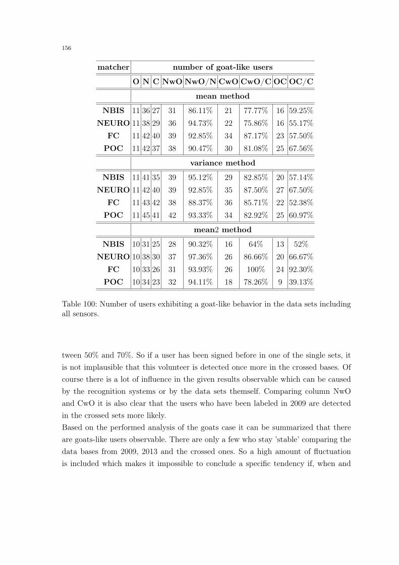
156

matcher number of goat-like users

O N C NwO NwO/N CwO CwO/C OC OC/C

mean method

NBIS 11 36 27 31 86.11% 21 77.77% 16 59.25%

NEURO 11 38 29 36 94.73% 22 75.86% 16 55.17%

FC 11 42 40 39 92.85% 34 87.17% 23 57.50%

POC 11 42 37 38 90.47% 30 81.08% 25 67.56%

variance method

NBIS 11 41 35 39 95.12% 29 82.85% 20 57.14%

NEURO 11 42 40 39 92.85% 35 87.50% 27 67.50%

FC 11 43 42 38 88.37% 36 85.71% 22 52.38%

POC 11 45 41 42 93.33% 34 82.92% 25 60.97%

mean2 method

NBIS 10 31 25 28 90.32% 16 64% 13 52%

NEURO 10 38 30 37 97.36% 26 86.66% 20 66.67%

FC 10 33 26 31 93.93% 26 100% 24 92.30%

POC 10 34 23 32 94.11% 18 78.26% 9 39.13%

Table 100: Number of users exhibiting a goat-like behavior in the data sets includingall sensors.

tween 50% and 70%. So if a user has been signed before in one of the single sets, itis not implausible that this volunteer is detected once more in the crossed bases. Ofcourse there is a lot of influence in the given results observable which can be causedby the recognition systems or by the data sets themself. Comparing column NwOand CwO it is also clear that the users who have been labeled in 2009 are detectedin the crossed sets more likely.Based on the performed analysis of the goats case it can be summarized that thereare goats-like users observable. There are only a few who stay ’stable’ comparing thedata bases from 2009, 2013 and the crossed ones. So a high amount of fluctuationis included which makes it impossible to conclude a specific tendency if, when and

157

probably why a volunteer can be marked as goat. But nevertheless the chances tosign a volunteer more than once is likely. Apart from these information it also can bestated that not all assumptions introduced in this Chapter 6 are confirmed. First ofall, the amount of fluctuation between the different goat-like volunteers is not thathigh as expected. Nevertheless it was possible to confirm that it is not unrealistic todetect a goat-like user once again in crossed data bases after marking this person inone of the single data sets before. Of course there is no certain answer if fingerprintageing or quality influences or even user dependent behavior are responsible for thedetected tendencies. But it was possible to prove that neither minutiae based finger-print recognition systems nor non-minutiae ones are outperforming the others in mostof the cases. All recognition systems display basically the same tendencies. For theused analysis methods an identical tendency can not be confirmed for all of them. Asassumed the minimum/maximum method is not suited for the goats analysis due totheir sensitivity to outliers. For the remaining methods (mean, variance and mean2)no crucial abnormalities are detected.

Lambs/Wolves analysis for time span excluding impostor scores: As thetitle of this section implies, two different analysis steps for the lambs/wolves analysisare discussed in the present thesis. According to the outcomes of Chapter 5 thereis a very high amount of stability corresponding to the impostor scores. Thereforeonly two cases were presented in more detail. The first one is excluding impostorscores which could be influenced by fingerprint ageing. So in fact this analysis is theequivalent to the WA method of the previous Chapter. The second one will be verysimilar to the HH analysis. The difference between the investigations presented inSection 6.4 and the HH method is the number of impostor scores which were takeninto account. That means that for the second lambs/wolves discussion all calculatedimpostor matching scores will be included and no repeated randomized selection ofthe scores performed. The reason for the chance is based on the before mentionedstability of the impostor scores.

Basically the lambs/wolves analysis was performed similarly compared to the goatsanalysis. With respect to the matching results, excluding correlation as described inSection 4.6, there will be no distinction between lambs and wolves in this master the-

158

number of no lambs/wolves-like users

NBIS NEURO FC POC

mean method 123 147 130 139


mean2 method 127 121 141 145

maximum sore method 148 122 146 150

Table 101: Number of users exhibiting no lambs/wolves-like behavior in the data setsincluding all sensors but using just impostor scores without time span information.

sis. So looking at the first result table, Table 101, it is clearly observable that thereis a difference to the results from the goats analysis. The big difference comparingthe first three methods and the maximum method can not be observed once again.Actually it seems that the maximum method is displaying similar or even a bettertendency. This enhancement is caused by the stability of the impostor scores. Thepresent fluctuations within the matching scores are not so high as for the genuine re-sults. So the lowest detectable number of users labeled as lamb or wolf can be derivedusing the NEURO matching results and the variance method. The displayed 106 userscorrespond to 54.08% of all volunteers within the data sets. The highest number ofusers which are never signed as lamb or wolf is 150 in the variance case using theNEURO and using POC for the maximum score method. For this purpose the marginbetween those who are never labeled as lamb or wolf in any data set, analysis andmatcher method is 22.45%. Compared to the goat margin it is much lower. So the highfluctuation in the goat case is also not detectable for lambs/wolves. It could be thatthe characteristics of a lamb- or wolf-like user are more distinctive on the one hand.The assumption seems to be a realistic one because of the stability of the impostorscores which has been detected in Chapter 5. On the other hand it is also possiblethat the similarity of the impostor results causes some problems for the recognitionof lamb/wolf-like users. The distinction between lamb/wolf or not lamb/wolf couldbe influenced because the outcomes of the analysis methods are related too much.For this purpose a low margin can also indicate that it is hard to distinguish betweentrue lambs/wolves and those who are normal in the sense of those animal types. Both

159

introduced interpretation are valid and there will be no further investigation basedon these hypothesis.As performed in the goat analysis, in Tables 102, 103,104 and 105 those lamb/wolf-like users which can be detected are displayed. The ’old’ data set corresponds againto the 2009 data set. The ’new’ data is the same as the data bases from 2013 andfinally the ’crossed’ set is based on the the crossing data bases from 2013 and 2009.It is easy to see that there were overlaps between the goats and lambs/wolf results.Nevertheless the first big difference to be mentioned between the goats and lambs/wolves set is the number of in totally labeled users. In most of the cases comparingthe information from Tables 91 and 101 there are more volunteers signed as lamb orwolf than as goat. To be more precise, in 12 of the displayed 16 cases, the numberof goats is lower than lambs/wolves. Especially interesting is that in 3 of the 4 caseswhere more goats are labeled the variance analysis method has been used. That couldbe a coincidence, but on the other hand this method could also be more suitable fordetecting goats or lambs/wolves. The main reason why this circumstance occurs willbe hard to detect because there are too many variables. The most important are theimprints contained in the data sets, the used sensor types, the fingerprint matchersystems and as a matter of course the variance method itself.Another interesting effect is the performance of the maximum analysis method. Inthe goat analysis this method performs very bad due to the sensitivity to outlierswithin the matching scores. At first sight the same problem is not detectable in thelambs/wolves analysis. In fact there are no big problems using this method duringthe further procedure because there is not such a high amount of fluctuations in theused matching scores compared to the goats case.

In opposition to the goats analysis in Tables 102, 103, 104 and 105 no specific abnor-mality can be observed. None of the four used analyzing methods was gathering anextremely low or high number of lambs/wolves. The only interesting observation canbe detected for the maximums method using NBIS and POC results.For both experiments the lamb/wolf-like volunteers in the all crossed, which havebeen detected, the users where the same as in 2009. This is possible of course, butwas not expected to be present. 3 volunteers, respectively 4, could be signed for thedata sets from 2013 as well. It seems that their score values were extraordinary uniqueto mark them more than once.

160

Data Set User ID

matcher NBIS

mean method

old 8, 47, 65, 86, 92, 98, 100, 130, 165, 166, 182

new 2, 10, 11, 13, 20, 24, 26, 27, 28, 30, 37, 38, 50, 51, 52,54, 55, 56, 59, 62, 63, 64, 69, 78, 79, 80, 85, 88,

90, 98, 100, 101, 104, 110, 111, 114, 118, 159, 167,178, 179, 180, 181, 187, 189, 194

crossed 6, 8, 9, 12, 23, 25, 39, 47, 49, 50, 52, 53, 56,57, 64, 75, 77, 78, 86, 87, 92, 98, 100, 109,

114, 139, 142, 144, 148, 162, 165, 166, 177, 178, 182

variance method

old 26, 39, 54, 71, 88, 129, 143, 158, 160, 165, 188

new 1, 2, 6, 10, 11, 13, 18, 22, 27, 28, 33, 35, 39, 40, 43, 45, 51,52, 54, 55, 56, 59, 60, 61, 79, 80, 81, 85, 88, 108, 113

120, 128, 135, 138, 141, 146, 148, 154, 155, 158, 159, 171,175, 181, 183, 185, 187, 193, 194, 195

crossed 5, 16, 21, 22, 25, 26, 27, 72, 80, 119, 129, 131, 132,134, 154, 158, 159, 160, 161, 162, 163, 170, 178, 187

mean2 method

old 8, 21, 25, 130, 131, 134, 162, 165, 166, 182

new 6, 10, 11, 13, 20, 27, 28, 38, 51, 52, 54, 55, 56, 64, 69,71, 74, 75, 78, 79, 80, 83, 89, 103, 104, 111, 112,115, 116, 122, 129, 136, 142, 146, 162, 164, 166,

167, 179, 180, 184, 185, 187, 194

crossed 8, 9, 12, 25, 49, 50, 53, 77, 78, 80, 81, 109, 110, 114, 129,130, 131, 134, 142, 144, 148, 160, 162, 165, 166,

177, 178, 182, 185, 186, 196

maximum sore method

old 8, 54, 109, 129, 160, 162, 165, 166, 182, 188

new 1, 6, 10, 11, 13, 19, 20, 22, 27, 28, 35, 38, 41, 51, 52, 54, 56,64, 69, 71, 74, 78, 79, 80, 85, 93, 111, 115, 116, 120, 130, 141, 142,

146, 155, 161, 162, 163, 166, 167, 179, 180, 187, 193, 194

crossed 8, 54, 109, 129, 160, 162, 165, 166, 182, 188

Table 102: User exhibiting a lamb/wolf-like behavior in the NBIS data sets includingall sensors but using just impostor scores without time span information.

161

Data Set User ID

matcher NEURO

mean method

old 54, 73, 74, 95, 130, 191, 192, 193, 194, 195, 196

new 10, 11, 27, 28, 34, 46, 51, 52, 54, 55, 62,79, 80, 97, 104, 138, 141, 165, 168,

178, 181, 185, 191, 192, 193, 194, 195, 196

crossed 9, 12, 25, 26, 36, 48, 49, 50, 53, 54, 56, 73, 74, 77, 78, 95,140, 143, 167, 180, 183, 191, 192, 193, 194, 195, 196

variance method

old 54, 73, 74, 95, 130, 191, 192, 193, 194, 195, 196

new 10, 11, 27, 28, 34, 46, 51, 52, 54, 55, 62, 79,80, 97, 104, 141, 165, 168, 178, 181,185, 191, 192, 193, 194, 195, 196

crossed 9, 12, 25, 26, 49, 50, 53, 54, 56, 73, 74, 77, 78, 95,99, 143, 167, 180, 183, 191, 192, 193, 194, 195, 196

mean2 method

old 40, 45, 54, 69, 73, 74, 75, 91, 95, 130

new 1, 2, 3, 4, 5, 10, 11, 16, 23, 27, 28, 33, 34, 37, 38, 46,51, 52, 54, 55, 62, 65, 70, 79, 80, 89, 97, 104,110, 112, 118, 138, 141, 142, 161, 162, 165, 168175, 178, 181, 185, 187, 192, 193, 194, 195, 196

crossed 9, 12, 25, 26, 36, 39, 40, 45, 48, 49, 50, 53, 54,56, 64, 69,73, 74, 75, 77, 78, 91, 95, 99, 130, 140, 143, 144, 163,

164, 167, 180, 183, 192, 193, 194, 195, 196

maximum sore method

old 40, 45, 54, 69, 73, 74, 75, 91, 95, 130

new 1, 2, 3, 4, 5, 10, 11, 16, 23, 27, 28, 33, 34, 37, 38,46, 51, 52, 54, 55, 62, 65, 70, 79, 80, 89,

97, 104, 110, 112, 118, 138, 141, 142, 161, 162,165, 168, 175, 178, 181, 185, 187

crossed 9, 12, 25, 26, 36, 39, 40, 45, 48, 49, 50, 53,54,56, 64, 67, 69, 73, 74, 75, 77, 78, 91, 95, 99,

130, 143, 144, 163, 164, 167, 180, 183

Table 103: User exhibiting a lamb/wolf-like behavior in the NEURO data sets includ-ing all sensors but using just impostor scores without time span information.

162

Data Set User ID

matcher FC

mean method

old 10, 41, 75, 133, 135, 148, 153, 160, 166, 182, 186

new 2, 3, 6, 7, 8, 10, 13, 18, 19, 20, 26, 29, 30, 34, 36, 38,43, 46, 53, 54, 58, 62, 63, 65, 66, 67, 73, 78, 85, 86, 99, 118,126, 137, 138, 139, 140, 151, 152, 156, 157, 182, 190, 192

crossed 1, 8, 10, 41, 56, 64, 65, 68, 75, 80, 92, 97, 103, 104, 130, 131,133, 135, 139, 140, 145, 148, 149, 151, 153, 160, 166, 182, 190

variance method

old 12, 15, 53, 77, 81, 90, 100, 102, 121, 127, 128

new 2, 4, 5, 7, 10, 11, 24, 35, 38, 42, 44, 46, 47, 51, 52, 57, 58,59, 66, 67, 68, 69, 70, 96, 97, 100, 103, 104, 105, 107,

112, 116, 118, 120, 126, 127, 133, 134, 142, 153,155, 163, 173, 174, 178, 180, 182, 187, 190

crossed 2, 5, 12, 15, 19, 41, 53, 77, 81, 85, 90, 100, 102,118, 121, 122, 127, 128, 144, 155, 163, 181, 182

mean2 method

old 19, 56, 92, 104, 148, 160, 166, 182, 184, 186

new 7, 10, 13, 14, 16, 26, 34, 36, 38, 46, 53, 54, 58, 62,72, 77, 78, 85, 86, 101, 103, 109, 114, 117, 118,

129, 137, 138,139, 140, 142, 150, 151, 166, 168, 182

crossed 15, 16, 34, 36, 56, 64, 79, 80, 88, 90, 92, 99, 102,103, 104, 116, 120, 121, 127, 130, 131, 139, 140,

148, 149, 151, 160, 166, 172, 182, 184

maximum sore method

old 25, 33, 50, 54, 92, 93, 148, 160, 166, 182

new 7, 10, 11, 13, 16, 26, 36, 38, 45, 46, 51, 52, 53, 54,55, 58, 62, 66, 77, 79, 80, 82, 84, 85, 86, 97, 101,103, 106, 110, 114, 137, 138, 139, 140, 142, 150,

157, 158, 159, 160, 161, 166, 182, 185, 189

crossed 15, 25, 33, 50, 54, 90, 92, 93, 102,109, 121, 127, 148, 160, 166, 182, 186

Table 104: User exhibiting a lamb/wolf-like behavior in the FC data sets includingall sensors but using just impostor scores without time span information.

163

Data Set User ID

matcher POC

mean method

old 25, 27, 50, 64, 71, 105, 108, 115, 122, 123, 153

new 6, 10, 12, 13, 14, 21, 22, 23, 38, 40, 51, 52, 60, 64, 74, 78,79, 105, 107, 121, 139, 143, 145, 151, 156, 169, 171, 183, 184,

188, 189, 190, 191, 192, 193, 194, 195, 196

crossed 8, 12, 16, 21, 22, 25, 27, 40, 49, 50, 62, 64, 76, 80, 105,108, 112, 123, 130, 149, 153, 169, 181, 189, 190, 191, 193, 195

variance method

old 40, 63, 66, 72, 75, 93, 95, 110, 125, 132, 136

new 1, 5, 6, 7, 10, 11, 15, 23, 24, 25, 30, 32, 33, 37, 38, 39, 46, 48,51, 52, 54, 55, 63, 66, 67, 74, 75, 80, 81, 94, 95,

100, 106, 111, 112, 119, 128, 137, 150, 158, 160, 168, 169, 173, 178,185, 186, 192, 196

crossed 1, 5, 6, 9, 12, 21, 22, 26, 49, 50, 51, 52, 53, 56, 65, 66,72, 75, 76, 84, 87, 93, 95, 97, 105, 110, 115, 124, 125, 132,

136, 160, 169, 188, 193

mean2 method

old 16, 25, 27, 50, 62, 64, 89, 115, 118, 130

new 1, 6, 10, 11, 12, 13, 14, 21, 22, 23, 24, 27, 35, 38, 40, 51, 52,54, 59, 60, 62, 64, 74, 78, 79, 80, 82, 98, 102, 119, 137, 139, 140,

150, 151, 160, 166, 168, 186, 188, 192

crossed 1, 6, 8, 10, 12, 16, 21, 22, 25, 27, 38, 40, 49, 50, 58, 62,64, 72, 76, 80, 84, 118, 130, 137, 138, 139, 149, 158, 186

maximum sore method

old 27, 40, 62, 73, 74, 93, 95, 115, 132, 136

new 5, 6, 10, 11, 12, 13, 15, 16, 21, 23, 24, 27, 37, 38, 40, 41, 51,52, 53, 54, 55, 57, 60, 62, 64, 67, 74, 79, 80, 98, 100, 111,

128, 137, 158, 159, 163, 168, 178, 188

crossed 27, 40, 62, 73, 74, 93, 95, 115, 132, 136

Table 105: User exhibiting a lamb/wolf-like behavior in the POC data sets includingall sensors but using just impostor scores without time span information.

164

matcher number of lamb/wolf-like users


mean method

NBIS 11 46 35 43 93.47% 25 71.42% 19 54.28%

NEURO 11 28 27 21 75% 17 62.96% 17 62.96%

FC 11 44 29 42 95.45% 19 65.51% 13 44.82%

POC 11 38 28 36 94.73% 20 71.42% 10 35.71%

variance method

NBIS 11 52 44 48 92.30% 36 81.81% 31 70.45%

NEURO 11 27 25 20 74.07% 15 60% 15 60%

FC 11 49 23 47 95.91% 12 52.17% 6 26.08%

POC 11 50 35 46 92% 26 74.28% 18 51.42%

mean2 method

NBIS 10 44 31 42 95.45% 22 70.96% 17 54.83%

NEURO 10 43 33 42 97.67% 23 69.69% 23 69.69%

FC 10 35 27 33 94.28% 19 70.37% 12 44.44%

POC 10 36 25 33 91.66% 17 68% 8 32%

maximum score method

NBIS 10 41 10 38 92.68% 0 - 0 -NEURO 10 43 32 42 97.67% 22 68.75% 22 68.75%

FC 10 42 12 38 90.47% 2 16.66% 2 16.66%

POC 10 40 10 36 90% 0 - 0 -

Table 106: Number of users exhibiting a lamb/wolf-like behavior in the data setsincluding all sensors, but using only time span excluding impostor scores.

Similar to the goats analysis the total number of lambs/wolves was analyzed as well,which is displayed in Table 106. In this table the same naming was used as in Table100. The influence of the lambs/wolves, detected in 2009, in the ’new’ and ’crossed’case is not very high. Basically in the 2013 data it is even lower compared to thegoats’ case. For the crossed data bases the opposite is detectable. For this purpose a

165

higher impact of the lamb/wolf-like volunteers, which have been marked in 2009, inthe crossed data sets as for the goats analysis can be stated. Furthermore a more orless stable amount of users, which have been signed in 2013, are responsible for thelamb/wolf observations in the crossed data using NBIS and NEURO. A different sit-uation is present for the two non-minutiae based fingerprint recognition systems. Forthose it seems that the lambs/wolves of 2013 are causing more of 50% of the retrievedusers. Based on those results it is possible to state not the assumed stability in caseof this first impostor score dependent volunteer analysis. This is the opposite of whatwas expected. It seems that regardless which animal type is considered an identicaltendency can be described. In fact there is a big difference between the goats andlambs/wolves case. This fluctuation is based on the non-minutiae fingerprint recogni-tion systems. Their results are much lower compared to the goats analysis. So it seemsthat in case of lambs and wolves the minutiae based approaches are better suited toretrieve and display the situation. It was also possible to get the information thatthe minimum/maximum method is delivering a different result for NBIS and POCcompared to the other two recognition systems. For all data sets the same volunteersin the old and crossed data bases could be signed. Additionally no correspondence tothe new data set was given. It will be interesting to see it the same results can bedescribed for the second lambs/wolves analysis once more.For the further analysis, the lamb/wolf-like users are separated according to matcher,analysis method and data sets. So in Tables 107, 108, 109, 110 and 111 the outcomesof the comparison between the 2009 and 2013 data, the 2009 and crossed data setsand the 2013 and crossed data sets are displayed. It is interesting to observe differenttypes of tendencies. The overall tendency is almost similar to the goats case, butlooking at the NEURO results an interesting difference can be detected.

In the Tables 107, 110 and 111 some problems are displayed, which occur usingthe NEURO impostor scores. There are six users, represented by ID 191, 192, 193,194, 195, 196, who are always signed for the mean and variance analysis method.Considering the circumstances this means that those are signed as lamb or wolf in2009, 2013 and the crossed data set. But they are never marked in any other menagerieanalysis method or in none of the other matching results. They are labeled as goat intwo single cases but are not interesting otherwise. There is a pattern that the signedusers have in common. This pattern is an important step of the mean and variance

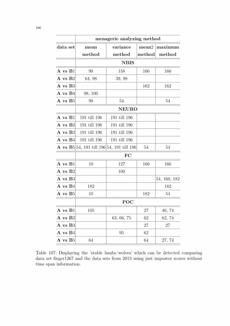
166


data set mean variance mean2 maximum


NBIS

A vs B1 98 158 166 166

A vs B2 64, 98 39, 98

A vs B3 162 162

A vs B4 98, 100

A vs B5 98 54 54

NEURO

A vs B1 191 till 196 191 till 196

A vs B2 191 till 196 191 till 196

A vs B3 191 till 196 191 till 196

A vs B4 191 till 196 191 till 196

A vs B5 54, 191 till 196 54, 191 till 196 54 54

FC

A vs B1 10 127 166 166

A vs B2 100

A vs B3 54, 160, 182

A vs B4 182 182

A vs B5 10 182 54

POC

A vs B1 105 27 40, 74

A vs B2 63, 66, 75 62 62, 74

A vs B3 27 27

A vs B4 95 62

A vs B5 64 64 27, 74

Table 107: Displaying the ’stable lambs/wolves’ which can be detected comparingdata set finger1267 and the data sets from 2013 using just impostor scores withouttime span information.

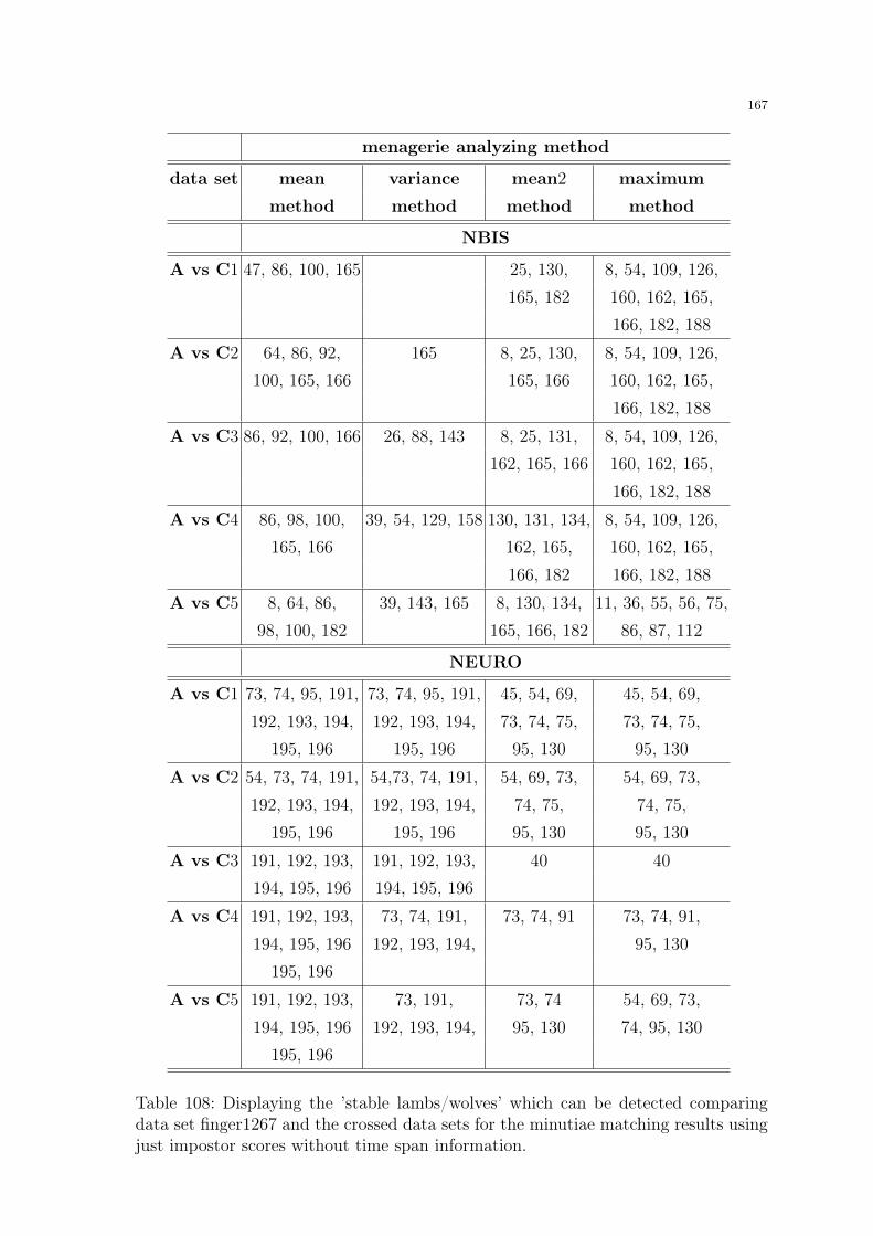
167




NBIS

A vs C1 47, 86, 100, 165 25, 130, 8, 54, 109, 126,165, 182 160, 162, 165,

166, 182, 188

A vs C2 64, 86, 92, 165 8, 25, 130, 8, 54, 109, 126,100, 165, 166 165, 166 160, 162, 165,

166, 182, 188

A vs C3 86, 92, 100, 166 26, 88, 143 8, 25, 131, 8, 54, 109, 126,162, 165, 166 160, 162, 165,

166, 182, 188

A vs C4 86, 98, 100, 39, 54, 129, 158 130, 131, 134, 8, 54, 109, 126,165, 166 162, 165, 160, 162, 165,

166, 182 166, 182, 188

A vs C5 8, 64, 86, 39, 143, 165 8, 130, 134, 11, 36, 55, 56, 75,98, 100, 182 165, 166, 182 86, 87, 112

NEURO

A vs C1 73, 74, 95, 191, 73, 74, 95, 191, 45, 54, 69, 45, 54, 69,192, 193, 194, 192, 193, 194, 73, 74, 75, 73, 74, 75,

195, 196 195, 196 95, 130 95, 130

A vs C2 54, 73, 74, 191, 54,73, 74, 191, 54, 69, 73, 54, 69, 73,192, 193, 194, 192, 193, 194, 74, 75, 74, 75,

195, 196 195, 196 95, 130 95, 130

A vs C3 191, 192, 193, 191, 192, 193, 40 40

194, 195, 196 194, 195, 196

A vs C4 191, 192, 193, 73, 74, 191, 73, 74, 91 73, 74, 91,194, 195, 196 192, 193, 194, 95, 130

195, 196

A vs C5 191, 192, 193, 73, 191, 73, 74 54, 69, 73,194, 195, 196 192, 193, 194, 95, 130 74, 95, 130

195, 196

Table 108: Displaying the ’stable lambs/wolves’ which can be detected comparingdata set finger1267 and the crossed data sets for the minutiae matching results usingjust impostor scores without time span information.

168




FC

A vs C1 10, 41, 75, 12, 15, 53, 56, 92, 104, 25, 33, 50,133, 135, 148, 77, 81, 102, 148, 160, 166, 92, 93, 148,153, 160, 182 182, 184 166, 182

A vs C2 41, 153, 166 12, 15, 53, 160, 166 25, 33, 50, 54,77, 81, 90, 100, 92, 93, 148,

102, 121, 127, 128 160, 166, 182

A vs C3 41, 75, 133, 12, 15, 53, 56, 160, 166 25, 33, 50, 54,153, 160, 166 77, 81, 90, 100, 92, 93, 148,

102, 121, 127, 128 160, 166, 182

A vs C4 41, 75, 15, 90, 102 56, 104, 166 25, 33, 50, 54,133, 153 92, 93, 148,

160, 166, 182

A vs C5 41, 75, 133, 12, 15, 53, 56, 92, 166 25, 33, 50, 54,153, 166 77, 81, 90, 100, 92, 93, 148,

102, 121, 127, 128 160, 166, 182

POC

A vs C1 25, 27, 105, 72, 93, 16, 25, 27, 50 27, 40, 62, 73,108, 123, 153 132, 136 74, 93, 95,

115, 132, 136

A vs C2 27, 64, 66, 75, 93, 27, 50, 64 27, 40, 62, 73,105, 123 95, 132, 136 74, 93, 95,

115, 132, 136

A vs C3 25, 27, 105, 75, 93, 95, 16, 25, 27, 50, 27, 40, 62, 73,123, 153 132, 136 64, 118, 130 74, 93, 95,

115, 132, 136

A vs C4 25, 27, 64, 72, 75, 93, 16, 25, 27, 27, 40, 62, 73,105, 123, 153 95, 110, 50,64 74, 93, 95,

125, 136 115, 132, 136

A vs C5 105, 123, 153 72, 136 16, 25, 27, 27, 40, 62, 73,52,64 74, 93, 95,

115, 132, 136

Table 109: Displaying the ’stable lambs/wolves’ which can be detected comparingdata set finger1267 and the crossed data sets for the non-minutiae matching resultsusing just impostor scores without time span information.

169




NBIS

B1 vs C1 185 166

B2 vs C2 64

B3 vs C3 162 162

B4 vs C4 98, 100

B5 vs C5 98 54

NEURO

B1 vs C1 191, 192, 193, 191, 192, 193,194, 195, 196 194, 195, 196

B2 vs C2 191, 192, 193, 191, 192, 193,194, 195, 196 194, 195, 196

B3 vs C3 191, 192, 193, 191, 192, 193,194, 195, 196 194, 195, 196

B4 vs C4 191, 192, 193, 191, 192, 193,194, 195, 196 194, 195, 196

B5 vs C5 191, 192, 193, 191, 192, 193,194, 195, 196 194, 195, 196

FC

B1 vs C1 10 166 166

B2 vs C2 65 100 103

B3 vs C3 65 34 54, 160, 182

B4 vs C4 155 182

B5 vs C5 190 54

POC

B1 vs C1 40, 105 27, 38, 40 40, 74

B2 vs C2 22, 193, 195 66, 75 22 62, 74

B3 vs C3 27 27

B4 vs C4 169 95 137, 139

B5 vs C5 12, 189, 1 10, 12, 64 27, 74190,191

Table 110: Displaying the ’stable lambs/wolves’ which can be detected comparingdata sets from 2013 and the crossed data sets using just impostor scores withouttime span information.

170




NBIS

A vs B1 vs C1 166

A vs B2 vs C2 64

A vs B3 vs C3 162 162

A vs B4 vs C4 98, 100

A vs B5 vs C5 98 54

NEURO

A vs B1 vs C1 191 to 196 191 to 196

A vs B2 vs C2 191 to 196 191 to 196

A vs B3 vs C3 191 to 196 191 to 196

A vs B4 vs C4 191 to 196 191 to 196

A vs B5 vs C5 191 to 196 191 to 196 54

FC

A vs B1 vs C1 10 166 166

A vs B2 vs C2 100

A vs B3 vs C3 54, 160, 182

A vs B4 vs C4 182

A vs B5 vs C5 54

POC

A vs B1 vs C1 105 27 40, 74

A vs B2 vs C2 66, 75 62, 74

A vs B3 vs C3 27 27

A vs B4 vs C4 95

A vs B5 vs C5 64 27, 74

Table 111: Displaying the ’stable lambs/wolves’ which can be detected in 2009, 2013and in the crossed data sets using just impostor scores without time span information.

171

method. Both are marking those volunteers which are below the 2.5 percentile andthose that are above the 97.5 percentile. This strategy is the reason why the six usersare only detected by these two methods. Especially the mean2 method is not able todetect them because only the users are labeled which mean score value is below the5 percentile.Apart from this abnormality it is hard to retrieve a certain tendency when a user islamb/wolf-like. Similar to the goats’ case no volunteer can be signed as the ’regular’lamb or wolf. It is even hard to mark those, which represent a ’stable’ behavior. Ofcourse it is possible to find them - introduced in Table 111, but they do not share aregularity.

Lambs/Wolves analysis for time span in- and excluding impostor scores:In particular there will not be another strategy for the second lambs/wolves analysis.The same concept was used to perform a similar analysis compared to the goatsand first lambs/wolves investigations. So no distinction between lambs and wolves ispresent as well.

number of no lambs/wolves-like users

NBIS NEURO FC POC

mean method 119 145 123 131


mean2 method 121 121 133 139

maximum sore method 126 122 136 137

Table 112: Number of users exhibiting no lambs/wolves-like behavior in the data setsincluding all sensors including all impostor scores.

In the first result table, Table 112, the number of those volunteer which were neverassigned to behave like the characteristic described in Section 6.3. Basically an ana-logical overall tendency like in the first lambs/wolves analysis can be measured. Thelowest amount of users labeled as lamb or wolf is detectable using the NEURO match-ing results and the variance method once more. Those 109 users represent 55.61%

172

of all volunteers which are included in the given data bases. Opposed to this lowerboundary, the highest number of users which were never signed as lamb or wolf is148. According to these information, the margin between those who are never labeledas lamb or wolf in any data set, analysis and matcher method is 19.90%. Comparedto the goat margin it is much lower again and slightly lower compared to the first

Data Set User ID

matcher NBIS

mean method

crossed 8, 9, 12, 23, 25, 31, 37, 39, 47, 49, 50, 52, 56, 57, 64, 75,77, 78, 80, 86, 87, 88, 92, 98, 100, 109, 134, 139, 144,

145, 148, 164, 165, 166, 168, 177, 178, 182, 183, 185, 196

variance method

crossed 6, 8, 9, 12, 15, 25, 26, 27, 31, 37, 40, 44, 45, 47, 49, 50, 53, 54, 55,56, 59, 60, 61, 63, 64, 70, 75, 77, 78, 117, 123, 128, 129, 134, 143,

145, 163, 165, 168, 170, 175, 182, 184, 185, 192

mean2 method

crossed 8, 9, 12, 18, 25, 40, 49, 50, 53, 76, 77, 78, 80, 81, 101, 109, 110,114, 124, 129, 131, 134, 144, 148, 161, 162, 164, 165, 166,

168, 177, 178, 182, 185, 186, 187, 196

maximum sore method

crossed 8, 9, 12, 13, 15, 25, 26, 40, 49, 50, 53, 56, 69, 76,77, 78, 80, 89,110, 113, 129, 134, 143,

144, 160, 163, 164, 165, 168, 182, 185, 186, 188, 196

Table 113: User exhibiting a lamb/wolf-like behavior in the NBIS data sets includingall sensors and impostor scores.

lambs/wolves analysis using only time span independent impostor scores. Also thehigh fluctuation in the goat case is also not detectable once more. Of course there isa small difference of 2.55% between both lambs/wolves margins. So it could be that

173

Data Set User ID

matcher NEURO

mean method

crossed 9, 12, 25, 26, 36, 48, 49, 50, 53, 56, 64, 73, 74, 77, 78, 95,140, 143, 167, 180, 183, 190, 191, 192, 193, 194, 195, 196

variance method

crossed 9, 12, 25, 26, 48, 49, 50, 53, 56, 64, 73, 74, 77, 78, 95,143, 167, 180, 183, 190, 191, 192, 193, 194, 195, 196

mean2 method

crossed 9, 10, 11, 12, 25, 26, 36, 37, 40, 48, 49, 50, 53, 54, 56,58, 64, 69, 73, 74, 77, 78, 91, 95, 99, 130, 140,143, 144, 163, 164, 167, 180, 181, 183, 187

maximum sore method

crossed 9, 10, 12, 25, 26, 37, 38, 48, 49, 50, 53,54, 56, 58, 64, 67, 69, 73, 74, 77, 78, 91, 95, 99,

130, 143, 144, 163, 164, 167, 180, 183

Table 114: User exhibiting a lamb/wolf-like behavior in the NEURO data sets includ-ing all sensors and impostor scores.

the combination of time span in- and excluding impostor scores is providing a morestable performance with regard to those two interesting matching behaviors.

In Tables 113, 114,115 and 116 the corresponding lamb/wolf-like users for using allimpostor scores were displayed. Because there is no chance in 2009 and 2013 impos-tor scores - the additional impostor scores are causing an effect on the crossed datasets, only those outcomes will not be displayed once more. They can be found in theTables 102, 103,104 and 105 in the first lambs/wolves analysis.In the following it is possible to find differences and similarities between those volun-teers and the users which have been detected in the lambs/wolves analysis of Section6.4. Nevertheless there won’t be a detailed discussion about the stable behavior of

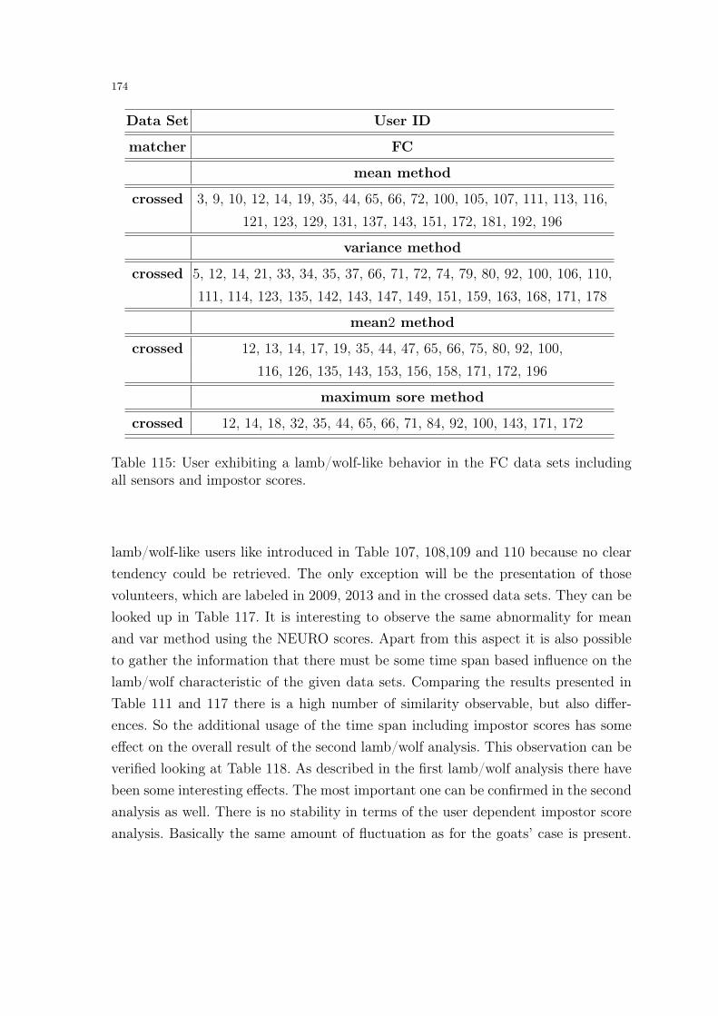
174

Data Set User ID

matcher FC

mean method

crossed 3, 9, 10, 12, 14, 19, 35, 44, 65, 66, 72, 100, 105, 107, 111, 113, 116,121, 123, 129, 131, 137, 143, 151, 172, 181, 192, 196

variance method

crossed 5, 12, 14, 21, 33, 34, 35, 37, 66, 71, 72, 74, 79, 80, 92, 100, 106, 110,111, 114, 123, 135, 142, 143, 147, 149, 151, 159, 163, 168, 171, 178

mean2 method

crossed 12, 13, 14, 17, 19, 35, 44, 47, 65, 66, 75, 80, 92, 100,116, 126, 135, 143, 153, 156, 158, 171, 172, 196

maximum sore method

crossed 12, 14, 18, 32, 35, 44, 65, 66, 71, 84, 92, 100, 143, 171, 172

Table 115: User exhibiting a lamb/wolf-like behavior in the FC data sets includingall sensors and impostor scores.

lamb/wolf-like users like introduced in Table 107, 108,109 and 110 because no cleartendency could be retrieved. The only exception will be the presentation of thosevolunteers, which are labeled in 2009, 2013 and in the crossed data sets. They can belooked up in Table 117. It is interesting to observe the same abnormality for meanand var method using the NEURO scores. Apart from this aspect it is also possibleto gather the information that there must be some time span based influence on thelamb/wolf characteristic of the given data sets. Comparing the results presented inTable 111 and 117 there is a high number of similarity observable, but also differ-ences. So the additional usage of the time span including impostor scores has someeffect on the overall result of the second lamb/wolf analysis. This observation can beverified looking at Table 118. As described in the first lamb/wolf analysis there havebeen some interesting effects. The most important one can be confirmed in the secondanalysis as well. There is no stability in terms of the user dependent impostor scoreanalysis. Basically the same amount of fluctuation as for the goats’ case is present.

175

Data Set User ID

matcher POC

mean method

crossed 1, 3, 12, 16, 25, 31, 41, 47, 48, 50, 62, 64, 71, 75, 76, 87, 104,115, 128, 137, 148, 149, 153, 158, 176, 189, 190, 193

variance method

crossed 1, 2,5, 8, 9, 10, 12, 14, 21, 22, 26, 30, 40, 49, 50,53, 65, 70, 72, 75, 76, 80, 87, 93, 95, 105, 110, 120,

123, 136, 142, 146, 176, 178, 196

mean2 method

crossed 10, 12, 16, 25, 27, 49, 50, 62, 64, 76, 104, 115, 118,126, 127, 128, 130, 136, 137, 138, 139, 8, 149, 158, 176, 180, 182

maximum sore method

crossed 7, 8, 9, 10, 12, 14, 21, 27, 40, 49, 50, 53, 65, 70,76, 93, 95, 98, 104, 132, 136, 137, 176, 186

Table 116: User exhibiting a lamb/wolf-like behavior in the POC data sets includingall sensors and impostor scores.

But it can not be stated if fingerprint ageing, quality or volunteer dependent influ-ences are responsible for this observation. Nevertheless it is likely - between 43.91%

and 16.67% - to detect a user marked as lamb or wolf in a crossed data base oncemore if the same one was signed in one of the single cases before. Of course thereare some variances based on the used fingerprint recognition system, the analysismethod and used data sets. But the majority of the reoccurrence likelihood is around30%. Besides, the abnormality in case of the minimum/maximum method for NBISand POC was not observable once again. All in all it seems that the influence of theprobably ageing related impostor matches is certainly detectable in the lambs/wolvesanalysis.

176




NBIS

A vs B1 vs C1

A vs B2 vs C2 64

A vs B3 vs C3

A vs B4 vs C4 98, 100

A vs B5 vs C5 98

NEURO

A vs B1 vs C1 191 to 196 191 to 196

A vs B2 vs C2 191 to 196 191 to 196

A vs B3 vs C3 191 to 196 191 to 196

A vs B4 vs C4 191 to 196 191 to 196

A vs B5 vs C5 191 to 196 191 to 196 54

FC

A vs B1 vs C1

A vs B2 vs C2 100

A vs B3 vs C3

A vs B4 vs C4

A vs B5 vs C5

POC

A vs B1 vs C1 27 40

A vs B2 vs C2 75

A vs B3 vs C3 27 27

A vs B4 vs C4 95 62

A vs B5 vs C5 64

Table 117: Displaying the ’stable lambs/wolves’ which can be detected in 2009, 2013and in the crossed data sets using all impostor scores.

177

According to the results displayed in Table 106 a weakness for the lamb/wolf be-havior in the crossed data sets was observable. The lamb/wolf users of 2013 wereinfluencing the detection of new lambs/wolves in the crossed data sets for FC andPOC. In the most cases much more than 50% of the signed lambs and wolves havebeen marked in 2013 before. On the opposite for NBIS and NEURO the impact couldbe located between roughly 30% and 46%. For the present second lamb/wolf analy-sis a different situation can be described: The time span including impostor scores’addition improves this impact. That means that the total number of lamb/wolf-likevolunteers, which are labeled in 2013 and who are marked in the crossed sets as wellis not that high as discussed for the first lamb/wolf analysis. To be more precise,in most of the cases between 20% and 30% of all 2013 lamb/wolf-like users can belabeled in the crossed data sets again. The only exception can be found for the mean2method using POC scores. But even in this case the total amount is lower than 50%.For this purpose it can be stated that more fluctuation within the location of thelambs and wolves is present. That means, it is not so likely to label a volunteer inthe 2013 and in the crossed sets. So using the present impostor data without timespan information causes a higher number of fluctuation in terms of reoccurrence ofthe signed users. Furthermore it was not possible to detect the abnormality basedon NBIS and POC using the maximum method. So there are other users signed in2009 and in the crossed sets. Especially the total number of them is not similar likeit could be described for the first lamb/wolf analysis.

After the menagerie analysis result description it is necessary to compare the goatand lamb/wolf cases a last time. As displayed in the goats analysis it was possible toobserve 5 different classes of user behavior. So the same classes can be detected inlamb/wolf analysis as well. There are volunteers, who are only signed in 2009, or 2013or in the crossed data set for example. Additionally having a look at the differencesand similarities of those two animal cases, another structure can be presented. Thisordering is taking into account that there are volunteers which are labeled not onlyonce. It is possible to detect four types of user tendency:

– Type 1: There are some users who are labeled just as ’goat’. As example for thiscase user 1 can be quoted using NBIS implementation and mean method.

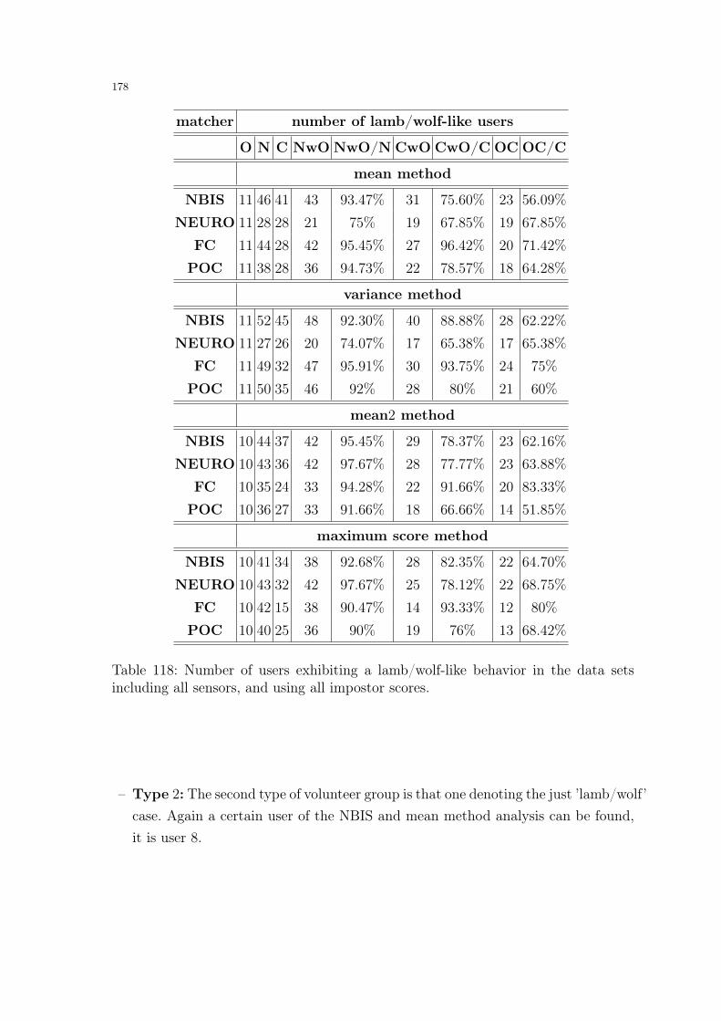
178

matcher number of lamb/wolf-like users


mean method

NBIS 11 46 41 43 93.47% 31 75.60% 23 56.09%

NEURO 11 28 28 21 75% 19 67.85% 19 67.85%

FC 11 44 28 42 95.45% 27 96.42% 20 71.42%

POC 11 38 28 36 94.73% 22 78.57% 18 64.28%

variance method

NBIS 11 52 45 48 92.30% 40 88.88% 28 62.22%

NEURO 11 27 26 20 74.07% 17 65.38% 17 65.38%

FC 11 49 32 47 95.91% 30 93.75% 24 75%

POC 11 50 35 46 92% 28 80% 21 60%

mean2 method

NBIS 10 44 37 42 95.45% 29 78.37% 23 62.16%

NEURO 10 43 36 42 97.67% 28 77.77% 23 63.88%

FC 10 35 24 33 94.28% 22 91.66% 20 83.33%

POC 10 36 27 33 91.66% 18 66.66% 14 51.85%

maximum score method

NBIS 10 41 34 38 92.68% 28 82.35% 22 64.70%

NEURO 10 43 32 42 97.67% 25 78.12% 22 68.75%

FC 10 42 15 38 90.47% 14 93.33% 12 80%

POC 10 40 25 36 90% 19 76% 13 68.42%

Table 118: Number of users exhibiting a lamb/wolf-like behavior in the data setsincluding all sensors, and using all impostor scores.

– Type 2: The second type of volunteer group is that one denoting the just ’lamb/wolf’case. Again a certain user of the NBIS and mean method analysis can be found,it is user 8.

179

– Type 3: If a volunteer is detected as goat and as lamb/wolf than it will belong tothis type. User 68 is one of those special ’animal’-users. The volunteer was labeledusing FC and the variance method.

– Type 4: Combining the information about non goat-like and non lamb/wolf usersleads to this last type. Within this list the lowest number of volunteers are in-cluded. In the NBIS and mean method results for example user 128 can be de-tected.

The total number of those volunteers belonging to one of the four types is displayed inthe following Tables 119 and 120. In Table 119 the score analysis without ageing influ-ence is displayed. The knowledge which was gathered from the second lambs/wolvesanalysis was taken into account and Table 120 describes this situation.As it is possible to see there are no specific tendencies or abnormalities observable.It seems that there is not a big difference comparing the matching results/menagerieanalysis methods and data sets. Of course there are fluctuations detectable, but all ofthem are caused either by the fingerprint recognition system, the menagerie analysismethod or the data sets themself. For example the outlier problem, present for themin/max method, is the most prominent variation in Tables 119 and 120. In par-ticular the differences between the both impostor score analysis investigations aredisplayed once more. But in general no certain tendency can be described.

6.5 Mean scores and System errors

Before performing a characterizing analysis concerning goats, lambs and wolves it isnecessary to discuss the before mentioned problems described in Section 6.3. Accord-ing to [40] there are several problems.Looking at the results of the goats and lambs/wolves analysis revealed an obvioussituation. The big difference between low matching scores and high ones cause sometroubles. Especially looking at the results provided by NBIS, NEURO and POC thesensitivity to outliers could be detected easily. So the gap within the highest andlowest matching scores introducing a number of so called outliers represents the mainproblem using the minimum/maximum analysis method. Therefore at a specific levelwithin the goats analysis this method was not used any longer. Opposed to this, thesame method was useful during the lamb/wolf analysis. So in the used data sets,

180

menagerie all all lambs/ only only lambs/ goats and never goat

method goats wolves goats wolves lambs/wolves or lamb/wolf

NBIS

mean 58 73 28 41 32 65

variance 70 90 37 55 35 36

mean2 51 69 22 40 29 76

min/max 110 48 77 28 20 38

NEURO

mean 63 49 46 33 16 84

variance 77 46 59 29 17 73

mean2 67 75 36 44 31 54

min/max 169 74 108 13 61 -

FC

mean 73 66 40 37 29 57

variance 71 64 43 43 21 61

mean2 65 55 49 33 22 76

min/max 59 50 43 37 13 87

POC

mean 74 57 40 27 30 65

variance 78 75 53 52 23 43

mean2 51 51 24 23 28 94

min/max 105 46 85 30 16 45

Table 119: Displaying the total number of users labeled as goat, or lamb/wolf or asboth ’animal types’ using only time span excluding impostor scores.

the high distinctiveness related to the genuine matching scores was a good attributelooking at the performance analysis, but not in case of the menagerie comparison.The second major problem is caused by the mean method. For sure the influence of theoutlier scores is not a problem in this case. So representing the user behavior withinthe given recognition system with the central moments of the genuine/impostor userscore distributions is a good idea on the one hand. But on the other hand the same

181

menagerie all all lambs/ only only lambs/ goats and never goat

method goats wolves goats wolves lambs/wolves or lamb/wolf

NBIS

mean 58 77 28 47 30 61

variance 70 87 37 54 33 39

mean2 51 75 22 46 29 70

min/max 110 70 77 37 33 16

NEURO

mean 63 51 46 34 17 82

variance 77 48 59 30 18 71

mean2 67 75 36 44 31 54

min/max 169 74 108 13 61 -

FC

mean 73 73 40 40 33 50

variance 71 82 43 54 28 43

mean2 65 63 49 47 16 68

min/max 59 60 43 44 16 77

POC

mean 74 65 40 31 34 57

variance 78 78 53 53 25 40

mean2 51 57 24 30 27 88

min/max 105 59 85 39 20 32

Table 120: Displaying the total number of users labeled as goat, or lamb/wolf or asboth ’animal types’ using all matching scores.

approach is vulnerable too. It is possible that no direct relationship between a user’smean score value and his/her participation in system errors is given. The detecteduser behavior to be a so called goat or lamb/wolf probably does not exist. It would beintroduced using the mean method. Therefore it is necessary to have a closer look atthis situation. It would be a significant problem if system errors would be introducedby almost all outliers. In this case the user’s mean average genuine and impostor

182

scores cannot be used as key number to detect false rejected/accepted user.

data set mean genuine score mean impostor score var genuine score var impostor scorevs false rejected vs false accepted vs false rejected vs false accepted

NBIS

A 0.7662 −0.4962 −0.3919 −0.3769

B1 0.7467 −0.4678 −0.3576 −0.3543

B2 0.7501 −0.4591 −0.3186 −0.3643

B3 0.8315 −0.4664 −0.3573 0.0309

B4 0.7084 −0.4720 −0.3839 0.0658

B5 0.7303 −0.4507 −0.3752 0.1162

C1 0.8740 −0.5118 −0.4823 −0.3964

C2 0.8969 −0.5100 −0.4609 −0.4144

C3 0.8964 −0.5128 −0.4904 −0.1840

C4 0.8664 −0.5127 −0.5087 −0.0398

C5 0.8750 −0.5060 -0.4771 0.0436

NEURO

A −0.5439 −0.4357 −0.5034 0.2536

B1 −0.5128 −0.4418 −0.5341 −0.0420

B2 0.7501 −0.5315 −0.4276 0.2423

B3 0.8315 −0.4908 −0.3639 0.3120

B4 0.7084 −0.5347 −0.4092 0.1761

B5 0.7303 −0.4921 −0.3649 0.2240

C1 −0.4748 −0.5263 −0.6534 0.1576

C2 −0.4721 −0.5216 −0.6367 0.2947

C3 −0.4636 −0.4881 −0.6327 0.3147

C4 −0.4775 −0.5088 −0.6125 0.1794

C5 −0.4711 −0.4912 −0.6308 0.2236

Table 121: NBIS and NEURO correlation based analysis’ results excluding time spanimpostor scores.

As said before, the outlier problem of the minimum/maximum approach is obviousand will not be discussed in more detail. On the contrary, the potential mean methodproblem will be evaluated more precise. Therefore the relation between the meanuser’s scores and the system errors has to be taken into account. This analysis de-pending on the score distribution must be performed for the genuine and the impostor

183

matching scores as well. Besides, to be on the safe side, because mean method andvariance method are related, the correlation based comparison was also performedfor the variance method.


FC

A −0.5439 0.5197 0.9168 −0.0005

B1 0.4861 −0.4418 0.9659 0.0168

B2 0.4845 −0.0644 0.9974 −0.0145

B3 0.5078 −0.0472 0.9928 0.0285

B4 0.4898 −0.0583 0.9950 −0.0099

B5 0.5066 −0.0317 0.9892 0.0010

C1 0.5174 −0.0243 0.8686 −0.1882

C2 0.5787 −0.0124 0.9913 −0.1836

C3 0.5773 −0.0088 0.9945 −0.1832

C4 0.5731 0.0442 0.9917 −0.2991

C5 0.5802 0.0007 0.9918 −0.1841

POC

A 0.9950 −0.5174 0.9995 −0.5335

B1 0.9996 −0.5024 0.9996 −0.5293

B2 0.9996 −0.5098 0.9996 −0.5370

B3 0.9996 −0.5039 0.9996 −0.5360

B4 0.9996 −0.5030 0.9996 −0.5278

B5 0.9996 −0.5082 0.9996 −0.5215

C1 0.9910 −0.5565 0.9910 −0.5701

C2 0.9930 −0.5586 0.9930 −0.5736

C3 0.9933 −0.5574 0.9933 −0.5737

C4 0.9936 −0.5566 0.9936 −0.5687

C5 0.9928 −0.5586 0.9928 −0.5666

Table 122: FC and POC correlation based analysis’ results excluding time span im-postor scores.

So the first part of this analysis must be on the one hand to calculate the user’s meanand variance average genuine/impostor scores. On the other hand the system errors,the number of falsely rejected or accepted users, have to be determined. This determi-

184

nation needs a certain threshold to distinguish between a system failure and a correctsystem decision. As introduced by [40] it is necessary to use a global threshold basedon the data set and the used matching method. Therefore the EER threshold waschosen. Subsequently for each user the same calculation was performed. The numberof genuine matches according to the user that are below this threshold are selected.They are representing the false rejected matches. Using the same method accordingto the user’s impostor scores the false accepted matches are selected.


NBIS

A 0.7662 −0.4962 −0.3919 −0.3769

B1 0.7467 −0.4678 −0.3576 −0.3543

B2 0.7501 −0.4591 −0.3186 −0.3643

B3 0.8315 −0.4664 −0.3573 0.0309

B4 0.7084 −0.4720 −0.3839 0.0658

B5 0.7303 −0.4507 −0.3752 0.1162

C1 0.8740 −0.6311 −0.4823 −0.5720

C2 0.8964 −0.6307 −0.4609 −0.5659

C3 0.8984 −0.6317 −0.4904 −0.3330

C4 0.8665 −0.6336 −0.5087 −0.1370

C5 0.8750 −0.6282 −0.4771 −0.0281

NEURO

A −0.5439 −0.4357 −0.5034 0.2536

B1 −0.5128 −0.4418 −0.5341 −0.0420

B2 0.7501 −0.5315 −0.4276 0.2423

B3 0.8315 −0.4908 −0.3639 0.3120

B4 0.7084 −0.5347 −0.4092 0.1761

B5 0.7303 −0.4921 −0.3649 0.2240

C1 −0.4748 −0.6827 −0.6534 0.0914

C2 −0.4721 −0.6762 −0.6367 0.3133

C3 −0.4636 −0.6263 −0.6327 0.2649

C4 −0.4775 −0.6606 −0.6125 0.1386

C5 −0.4711 −0.6424 −0.6308 0.1721

Table 123: NBIS and NEURO correlation based analysis’ results using all scores.

185


FC

A −0.5439 0.5197 0.9168 −0.0005

B1 0.4861 −0.4418 0.9659 0.0168

B2 0.4845 −0.0644 0.9974 −0.0145

B3 0.5078 −0.0472 0.9928 0.0285

B4 0.4898 −0.0583 0.9950 −0.0099

B5 0.5066 −0.0317 0.9892 0.0010

C1 0.5174 −0.5606 0.8686 −0.6938

C2 0.5787 −0.5608 0.9913 −0.6792

C3 0.5773 −0.5572 0.9945 −0.6858

C4 0.5731 −0.5590 0.9917 −0.6860

C5 0.5802 −0.5524 0.9918 −0.6825

POC

A 0.9950 −0.5174 0.9995 −0.5335

B1 0.9996 −0.5024 0.9996 −0.5293

B2 0.9996 −0.5098 0.9996 −0.5370

B3 0.9996 −0.5039 0.9996 −0.5360

B4 0.9996 −0.5030 0.9996 −0.5278

B5 0.9996 −0.5082 0.9996 −0.5215

C1 0.9910 −0.7143 0.9910 −0.7141

C2 0.9930 −0.7142 0.9930 −0.7129

C3 0.9933 −0.7129 0.9933 −0.7107

C4 0.9936 −0.7123 0.9936 −0.7093

C5 0.9928 −0.7112 0.9928 −0.7084

Table 124: FC and POC correlation based analysis’ results using all scores.

After this first step, preparing the needed information of the recognition systemthe Pearson product-moment correlation coefficient was calculated for each data set.The correlation value is used to display the linear relationship between two or moredata sets or random variables. In this case the linear relationship between the user’smean/variance genuine/impostor scores and the detected system errors was calcu-lated. Since four matching implementations and eleven different data sets have beenused in this master thesis, the analysis had to be executed for all possible combina-tions between recognition systems and data sets. The statistically significant resultsat the 0.01 level can be found in Tables 121, 122, 123 and 124 for the mean and the

186

variance method. As can be seen in those tables, the linear relationship between theuser’s average mean and variance scores and the system errors is detectable in all datasets and matcher types, despite there is not always an identical tendency observable.So only for the POC results the correlation between mean/var genuine scores and falserejected matches is positive across all data bases and negative for the mean/var im-postor scores compared to the false accepted matches. In all other cases this tendencyis chancing depending on the data set and the recognition method. But not only thisfluctuation can be looked up. The strength of the correlation is also not consistent. Insome cases a very high positive correlation can be detected and sometimes a very lownegative one as well. Nevertheless the linear correlation can be detected for each dataset and matcher type and this information guarantees that the analysis concerningthe mean and variance zoo method is consistent according to the actual system errors.

6.6 Menagerie Analysis and Ageing Effects detected in Section 5

The investigations that have been performed in Section 5 yield to an interesting out-come. The shift in the genuine score distributions to the left, the decrease of thehigher genuine scores and the increase of the lower ones indicated a first effect thatcould be initiated by ageing.In this part of the current thesis the aim will be to combine the information of Section5 and the menagerie analysis introduced in Section 6. Since the shift in the genuinescore distribution could be verified the main task is to have a look what does thismean for ’Doddingtion’s Zoo’. On the other hand the almost stable impostor scoredistribution will be taken into account if this stability could be used as reference incase of looking at menagerie ageing effects.At first the focus will lie on the genuine score distribution and the genuine scorerelated goats analysis. The results of the first experimental setup are quite clear. Be-cause the decrease in the genuine scores is unmistakable the impression is that theremust be an effect detectable in the goats analysis as well. As introduced in Section 6.1the goat’s characteristic is related to low genuine scores. That would lead to the sug-gestion that due to the fact the number of low genuine scores is raised in the crosseddata sets compared to the single data sets, also the number of detected goats mustincrease too. But, as readable in Table 100 a different observation can be detected.To be more precise, the total number of goats in the crossed data sets is higher as in

187

the older data set from 2009 and lower as in the younger data sets from 2013. Havinga even closer look at the results, the number of users labeled as goats is always iden-tical for each set. This outcome seems to be a contradiction to the direct relationshipbetween low genuine scores and the definition of goats. To solve the contradiction itis necessary to think once again what is done while performing the menagerie analysis.

Basically the idea of the menagerie analysis is, to have a look how many users areincluded and than have a look at the matching scores. Those users who have the lowestpercentage of matching scores are labeled as goat or lamb or wolf. This methodologyis performed for each data set independently. So there is no information about whatscores are available in which data base. So the lowest percentage of matching scoreswill be the same for each set, but the lowest scores may differ a lot. Look at thefollowing example. Consider two different data bases. In the first one the matchingscores are located between 0.5 and 1 and in the other case between 0 and 0.6. It isobvious that the matching scores in the first data set are higher than in the otherexample set on average. So the user depending matching scores in the first set willalso be higher on average. Therefore it is clear that roughly summarized the lowestuser depending scores will be also higher. But for each set the same percentage willbe used to label the ’animals’. So the marking is not connected directly to the size ofthe scores. Of course the scores are used to build up the selection basis to separate theusers, but they are not involved during the labeling process. Therefore the results fromSection 6.4 cannot be used to indicate the outcomes of the experiments described inSection 5 and vice versa concerning the genuine scores. The shift in the genuine scoredistributions and the decrease of the total number of goats in the crossed data setsare both independent from each other. Both are ageing effects, but effects dependingon different experimental setups.But nevertheless there are some goats depending aspects detectable that can besummarized to be ageing effects in case of menagerie analysis concerning the goatdefinition. First depending on the data sets it is possible to label certain users moreoften than others independently from the used matching method. For example user 6and 25 are detected more often as for example user 194. It seems that there are somevolunteers which are prone to get low genuine matching scores. Especially because ifthis user is labeled once in the old data set it is very likely to detect the same volunteerin the newer data sets and the crossed data sets as well. Opposed to this the chance

188

to label a user in the crossed data sets if the volunteer was not labeled before isvery rare. The second interesting observation is that there are some volunteers whoare labeled in the old data set, but never again or in one of the new data sets andnever again. For example user 14 and 44 in the NEURO results for variance analysismethod or user 107 using FC and the mean method. So roughly spoken it is possibleto summarize the ’goatish’ behavior and create three classes:

– Goat-free Class: Not detected as goat in the old data set indicates a very highpossibility to be never labeled as goat.

– Goat-stable Class: Labeled once in the old data set indicates a very high pos-sibility to be labeled as goat again in a crossed data base.

– Goat-once Class: Those users who are labeled just once, which can be explainedfor example by ageing.

Nevertheless it also must be summarized that the assumption of detecting a veryhigh amount of fluctuation within the goat-like volunteers could not be confirmed.According to the high amount of variance comparing the single and crossed datasets’ genuine scores it was expected that in case of the corresponding goats’ case veryhigh fluctuation can be observed as well. Which would be indicating that a probablypresent fingerprint ageing is causing variances in terms of the goats characteristic.Users who are marked as goats in a specific year would not retain this characteristicacross several years. But according to the results of the performed experiments thishypothesis must be rejected. There are certain volunteers who extend their goat-likebehavior over several years. This effect can be caused by ageing. But as describedin the enumeration above not only those ’stable-goats’ seem to be influenced by aprobably detectable ageing. It is also possible that fingerprint ageing is responsiblefor the fact that some volunteers are loosing their goat characteristic. Of course thosewho are labeled only once can also be signed by accident because of some failureduring the matching procedure or by some problems during the imprint acquisition.This quality based aspect will be discussed in the following Chapter 7.The second interesting outcome from Section 6 was the almost stability of the im-postor score distributions and on the other hand the decrease of the total number oflambs/wolves in the crossed data sets compared to the new data sets as described inthe corresponding analysis’ results. This decrease, which can be detected comparingthe entire amount of lambs/wolves in Tables 106 and 118, indicates that the variabil-

189

ity of lamb/wolf-like users in the new data sets together is much higher compared tothe crossed data sets. So despite the fact that the impostor score distributions seemto be more or less stable across the data sets there is an impact on the volunteerbehavior. Especially comparing those lambs/wolves which are detected for FC andPOC the first time in 2013 and once more in the crossed sets. It seems that usingall impostor scores a more stable behavior is present. In particular the impact of thetime span including impostor scores is most observable in this situation. The out-comes are more similar to NBIS and NEURO after all impostor scores were takeninto account. For this purpose ageing could have an impact on the described aspect,but so far it could also be that the quality of the imprints is responsible as well be-cause they could also influence the recognition performance of the used fingerprintrecognition systems. Additionally it was very interesting to observe that there wasmore fluctuation as assumed in the lamb/wolf case. Due to the stability of the im-postor scores a quite high amount of stability was expected for this characteristic aswell. The number of stable lambs/wolves as detected in the experiments is a littlebit lower as assumed. Of course the results display the a high chance of extendingthe users’ lamb/wolf characteristic, but it is interesting to observe that there is a lotof correspondence to the goats case. It seems that the likelihood of an animal-likebehavior extension is more or less same for both investigated animal cases.Furthermore it is possible to say that there are basically the same classes observableas described above using the goat information. But it can be stated that there aremuch more users which can be grouped in a so called ’Lamb/Wolf-once Class’. Due tothe fact that the lamb and wolf case is taken into account together it is not possibleto say if the lamb-like characteristics are providing the high number of fluctuationor the wolf-like. So from this point of view it is also not possible to state if due tothe variability - caused by ageing - a system weakness is detectable. This would needsome further investigations, which would exceed this thesis.Apart from this fact it will be interesting to see how important the impact of thequality aspect of the imprints is influencing the performed experiments so far. Thequality analysis can be looked up in the following Section 7.

190

7 Fingerprint Ageing and Quality

In this final section of the master thesis a discussion about the quality informationof the imprints will be taken into account because the performance of a fingerprintrecognition system is affected by the quality of the imprints in the data base. Soprobably it is possible to explain the detected effects concerning the performance andmenagerie analysis which have been discussed in Chapters 5 and 6. One question willbe if the quality is influencing the possibility to assign a specific animal type to acertain user than it is not possible to speak of an ageing effect. But on the otherside if quality has no impact on the menagerie recognition than the present chancesdetected in the analysis before are affected by ageing. Besides, it is also important todiscuss if the outcomes of Chapter 5 can be explained by this analysis or not. So itwill be interesting to see if the results are representing the results from [41] or not.Apart from the before mentioned [41] there are some very interesting effects thatneed to be discussed first, before starting to talk of certain quality measurements.One aspect is the sensor specific point of view. Results about cross-sensor matchinghave been presented in [7]. Using a multi-sensor data base, where for the same volun-teers fingerprint images have been acquired with different sensors types. So the setupis similar to the data sets that are used in this master thesis. Of course the numberof sensors included in the particular data set is higher in the data bases introducedfor this thesis. In [7] it was possible to detect an increase of the user quality valuesfor two single sensor types. At the same time the threshold value for the EER wasraised as well. In the other case there was no increase or decrease detectable. Fus-ing the different sensors a high reduction of the EER could be observed. So it seemsthat fusing two sensor types can improve the performance independent of the imprintquality. The used matching algorithm was the NBIS implementation. Because in themulti-sensor data base no time span is included, it is hard to compare the resultswith the outcomes of the quality analysis of this thesis, but it is interesting to keepthe information in mind if abnormalities occur.Another interesting circumstance is discussed in [21]. As displayed in Section 4.4there have been different acquisition conditions for the used data sets. One of themost eye-catching problems during the acquisition process is the fingerprint force.That means the different strength of pressure the finger is pressed on the sensorplate. This circumstance was considered into more detail in [21]. Selecting different

191

so called force levels it was possible to detect an impact of different pressure and thecorrelation to the imprint quality and minutiae detecting ability. They also used theNBIS fingerprint recognition system as well.So it seems that the quality of imprints is influenced by a variety of conditions. There-fore to realize the quality analysis of Doddington’s zoo results and the data base ingeneral, different quality measurements will be taken into account. The results of themethods should be compared to verify that there is no quality method dependentdeviation. Besides, because there are different strategies that can be used to retrievequality information of an imprint it was necessary to select some specific methodolo-gies. Basically it is possible to divide those theoretical concepts into 2 classes. Firstthere is the class containing the ideas that are focusing on local features to describethe quality of an imprint. On the other side there is the second class containing globalfeature based measurements. In [6] there has been a study to compare the qualityapproaches and additionally a third class was also considered. This introduced thirdclass is including all strategies that are addressing the quality problem to be a clas-sification issue.Due to the fact that the NIST Fingerprint Image Quality 2.0 (NFIQ 2.0) was notreleased the time the quality experiments have been performed, following methodshave been taken into account:

– NIST Fingerprint Image Quality (NFIQ)

– Image Quality of Fingerprint (IQF)

– Gabor Filter Image Quality of Fingerprint (GFIQF)

According to the named quality measurements it is possible to characterize thosemethods. Especially the strategy to retrieve the needed information to compare thequalities of the imprints is important. The NFIQ implementation, introduced in 2004

is using minutiae feature information to gather the quality values. The more detaileddiscussion of this method will be in Subsection 7.1 and is based on [36].The second method, the IQF implementation, is based on using the Fast FourierTransform to select certain parameters of the power spectrum. In Subsection 7.2,after describing the NFIQ, this methodology will be analyzed. The main informationtherefore can be looked up in [26].The last measurement is based on Gabor Filter application. The concept for the

192

methodology was presented in [34] and will be discussed in Subsection 7.3.

7.1 NIST Fingerprint Image Quality (NFIQ)

This first method was developed and implemented at the National Institute of Stan-dards and Technology it is part of the before used NBIS software package. This stan-dard fingerprint quality measurement was introduced in 2004 by several researchers,Elham Tabassi among others [36]. The main idea was to improve the performance ofa fingerprint recognition system. So for example imprints with poor quality can beprocessed using different algorithms or thresholds or the imprint is acquired and thequality value is to low another imprint could be enrolled more easily. But to be ableto perform those tasks a specific quality measurement was mandatory. There are twomain steps that must be executed to gather the NFIQ value of an imprint.

– Feature extraction: In the first step the mindtct implementation is used toextract the needed features. Basically the same mindtct algorithm is used as inthe NBIS software package. But there is a slight adaptation concerning the num-ber of extracted minutiae information. Compared with original feature extractionmethod the dimension of the feature vector is restricted to 11 for each imprint.In the classical implementation this restriction is not included and the length ofthe feature vector can vary. The selected minutiae are the 11 most important anddistinctive ones.

– Classification: After the feature extraction the feature vectors are forwarded toa neural network to classify the input information into five different classes. Eachclass is representing a separate quality value. Those values are varying between1, the best quality measurement and 5, the poorest imprint quality that can beselected with the NFIQ software.

In [36] different characteristics for low quality values have been observed. The mostimportant are distortion caused by the fingerprints itself, like scars or distortion thatoccurred during the acquisition or compression process.Based on this quality measurement method the first calculation performed on the datasets was to gather an average quality value for all data sets. As visible in Table 125it is not possible to detect any specific data set dependent abnormality. Nevertheless

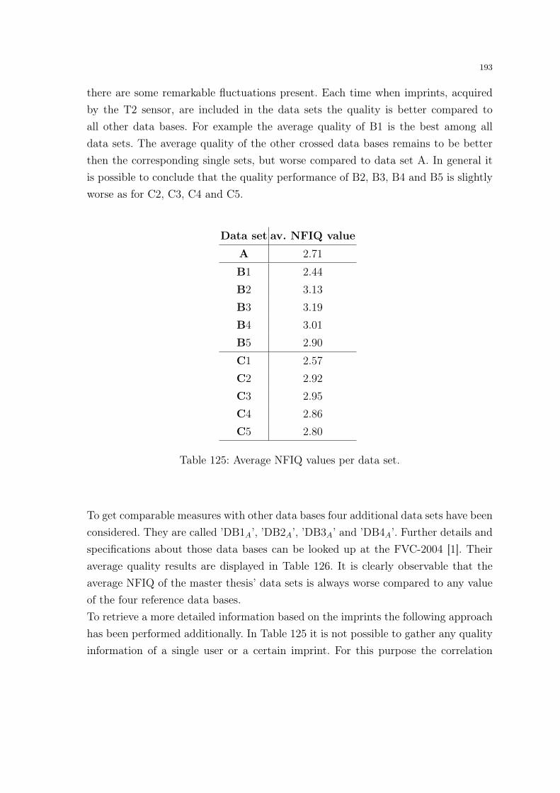
193

there are some remarkable fluctuations present. Each time when imprints, acquiredby the T2 sensor, are included in the data sets the quality is better compared toall other data bases. For example the average quality of B1 is the best among alldata sets. The average quality of the other crossed data bases remains to be betterthen the corresponding single sets, but worse compared to data set A. In general itis possible to conclude that the quality performance of B2, B3, B4 and B5 is slightlyworse as for C2, C3, C4 and C5.

Data set av. NFIQ value

A 2.71

B1 2.44

B2 3.13

B3 3.19

B4 3.01

B5 2.90

C1 2.57

C2 2.92

C3 2.95

C4 2.86

C5 2.80

Table 125: Average NFIQ values per data set.

To get comparable measures with other data bases four additional data sets have beenconsidered. They are called ’DB1A’, ’DB2A’, ’DB3A’ and ’DB4A’. Further details andspecifications about those data bases can be looked up at the FVC-2004 [1]. Theiraverage quality results are displayed in Table 126. It is clearly observable that theaverage NFIQ of the master thesis’ data sets is always worse compared to any valueof the four reference data bases.To retrieve a more detailed information based on the imprints the following approachhas been performed additionally. In Table 125 it is not possible to gather any qualityinformation of a single user or a certain imprint. For this purpose the correlation

194

between the single quality impact of the imprints will be discussed in a more detailedway. The results of these experiments can be looked up in Section 7.4.

Data set av. NFIQ value

DB1A 1.34

DB2A 2.31

DB3A 1.66

DB4A 1.81

Table 126: Average NFIQ values of the FVC-2004 data sets.

7.2 Image Quality of Fingerprint (IQF)

The Image Quality of Fingerprint (IQF) software4 is an application to measure visualquality of fingerprint images. The IQF implementation is based on the IQM imple-mentation of MITRE, a non-profit research corporation. IQM is the abbreviation forImage Quality Measure what was developed as a quality measure for arbitrary im-ages. The basic method behind both quality measures is the use of information thatcan be gathered in the Fourier domain. Therefore the most important calculationsteps of the IQF measure, that are based on [26], are the following:

– Windowing and Fast Fourier Transformation: An input image is dividedinto overlapping windows first. For each of those sub- images the two dimen-sional Fast Fourier Transformation (FFT) is computed. To improve the accuracyof the implementation the sub-image power spectra are normalized taking the totalpower spectrum of the entire imprint into account and the area of the sub-imagesas well.

– Filtering: The calculated normalized power spectra are filtered in the second step.According to [26] a human visual system filter (HVS) is used because the qualitymeasure should represent the human quality impression of an imprint. For that itis necessary to take care of spatial and temporal patterns the human visual system

4 http://www2.mitre.org/tech/mtf/

195

is sensitive to which is provided using a HVS. So basically a HVS is a filter whichhas more or less similar characteristics to a low pass or band pass filter because inthe human visual system the limited number of rods exceed the number of cones.So the high frequency information can not be used that good compared to lowerfrequencies. Based on this information during the filtering step the high frequencyinformation of the normalized power spectra is cut off. The remaining entries ofthe normalized filtered power spectra sub-images are summed up. So for eachsub-image one single value, the sub-image quality value, is derived. After thosesingle quality values for each sub-image have been found they are compared toeach other. The highest quality entry is selected. All other values are not neededanymore because the real IQF quality values is just based on that sub-image whichcontains the highest number of low frequency information.

– Quality Calculation: The final calculation step is performed on the detectedsub-image which was introduced in the filtering step. The output values will bebased not only on using the low frequency information, but also on more contrastinformation. So the quality value of the selected sub-image is normalized using thezero frequency power of the same sub-image. According to [26] this zero frequencynormalization (dc normalization) could lead to overestimation of the output valueif the entire fingerprint image is quite dark and to underestimation in case theimprint is a light one. To compensate this effect a weighting of the dc normalizedquality value will be performed. That means that the actual value will be multi-plied by the squared average gray level of the sub-image. After this multiplicationthe final output quality value is derived in the most cases. If the entire imprint is avery high contrast one or a very light image some additional adjustments must beperformed. Otherwise for the high contrast case a overestimation of the IQF valuewould happen and a underestimation for the light image case. The adjustment isan additional multiplication with 0.17 for the high contrast specification and 2.5

for the other one. The idea behind is to mitigate the dc normalization step.

As described in [26] the output values are ranged between 0 and 100. The higherthe quality value of an imprint gets, the better the quality of the fingerprint imageis using this method. It will be interesting to compare the results with the otherquality measurement methodologies because this method was designed to give qualityfeedback based on the human quality impression.

196

Based on the calculated IQF values, similar to the NFIQ calculation, the averageIQF values for the single data sets has been derived. As visible in Table 127 thereis no abnormality detectable. Those results display a slightly different tendency asdetectable for the average NFIQ results that have been introduced in Table 125.

Data set av. IQF value

A 12.26

B1 9.79

B2 12.39

B3 12.14

B4 12.10

B5 12.29

C1 11.02

C2 12.32

C3 12.20

C4 12.18

C5 12.27

Table 127: Average IQF values per data set.

Data set av. IQF value

DB1A 9.31

DB2A 6.71

DB3A 8.52

DB4A 3.88

Table 128: Average IQF values for the FVC-2004 data sets.

Similar to the NFIQ case the average IQF values for the introduced four referencedata sets have been calculated as well. The corresponding results, which are displayedin Table 128, reveal that the IQF of the used data bases A to C5 is better compared

197

to those reference data sets.Independently from the similarity of the average IQF and the NFIQ results it is alsoclearly observable that the there is a difference regarding the quality measure good-ness. As introduced the output of the NFIQ measurement is a number between 1 and5. Where 5 is the worst result an imprint can receive. The values of the IQF measureon the other hand is displayed using a number between 0 and 100 for each imprint.In this case the higher the value is the better the quality of the fingerprint image.Comparing the results thinking about this background information it is clear that theaverage IQF results are indicating that the imprints have a much worse quality thanthe NFIQ values provide. It seems that the impact of designing a quality measurebased on the human quality impression is high on the used data sets. Additionallythe IQF results display a quite bad quality of all data sets, so the tendency is thesame one as compared to NFIQ.Due to this circumstance it will be interesting to see how the IQF results for the av-erage false accepted and rejected quality analysis, as introduced in the NFIQ sectionof this master’ thesis, look like. They are displayed and discussed in Section 7.4.

7.3 Gabor Filter Image Quality of Fingerprint (GFIQF)

The Gabor Filter Image Quality of Fingerprint (GFIQF) is the third quality measure-ment method that has been taken into account for this master thesis. As opposed tothe other two software applications for this method no free available implementationscould be found. Therefore it was implemented based on [34]. As the name implies,the basic idea behind this method is the use of Gabor Filters. According to [34] themain steps can be summarized as follows:

– Imprint division into non overlapping blocks: Each input image is divided ina set of blocks. Each block has the same size of nxn and they are not overlappingeach other. For the experimental setup the block size of 16x16 pixel was used. Thedimensions have not been chosen arbitrary, they are based on the one hand on thesimilarity to the setting introduced in [34]. On the other hand they are based onthe dimensions of the fingerprint images. Due to the dimensions of 328x356 and256x360 as discussed in Section 4.1 and Section 4.2 it was not possible to dividethe imprints uniformly. There would have been a few blocks only consisting of asmall number of pixels. Therefore the border pixels have been cut off to fulfill the

198

task of creating regular blocks of each imprint. The cut off is not a big problembecause no quality dependent information is located there.

– Gabor Filtering and feature calculation: On each of the before introducedblocks a set of 8 Gabor Filters is applied to. There are a few important informa-tion necessary for this calculation step. As displayed in [34] the main parametersare the total number of orientations and the orientations itself and the frequencyof the sinusoidal plane wave of the Gabor filters. The orientations θ that havebeen chosen are π

8, π

4, 3∗π

8, π

2, 5∗π

8, 3∗π

4, 7∗π

8and π. The idea was to capture as

much orientation information as possible and therefore those have been selected.The frequency of the sinusoidal plane f wave was set to 1

4. Just like the before

mentioned parameters, the characteristics for the standard deviations along thex- and y-axes have been determined empirically. The standard deviation alongthe x-axes σx was set to 4 and along the y-axes σy was set to 2. The result of thefiltering process are 8 Gabor feature sets.

– Gabor standard deviation calculation: Based on the Gabor features the socalled Gabor standard deviation is calculated as third part of this quality imple-mentation. This standard deviation is measuring the amount of variation withinthe Gabor features. So the calculated features are following a distribution based onthe 8 Gabor filtered block information and for each block one standard deviationvalue is derived. It is mandatory for the final calculation step.

– Quality Index (QI): The standard deviation values are used for two differentapproaches. The first one is to separate between foreground and background in-formation. Due to the circumstance, that in a fingerprint image at the locationwhere the imprint can be located a high number of edges is detectable, the Gaborfeatures are useful to distinguish between imprint and background. If the stan-dard deviation is less than a particular threshold T1 than the block is marked asbackground.The second approach is the actual imprint quality measurement. For this purposeonly the foreground blocks are taken into account. If the standard deviation of aforeground block is less than a threshold T2 than this block is labeled as a poorforeground block. Those poor foreground block are used to calculate the Quality

199

Index (QI) of the imprint:

QI = 1− number of poor quality foreground blockstotal number of foreground blocks

(1)

Looking at the formula above how the QI is calculated it is clear that a high numberof poor quality foreground block is indicating a bad result. So if the QI is low thismeans that the quality of the fingerprint image is not good. Basically a QI value near1 describes a image which has a good GFIQF value. The worst possible value is 0.Using the described method, the same approach as performed for the NFIQ and IQFquality measures has been done. Therefore the average GFIQF of the used data setscan be looked up in Table 129.

Data set av. GFIQF value

A 0.1631

B1 0.8311

B2 0.1290

B3 0.1921

B4 0.0976

B5 0.0686

C1 0.4971

C2 0.1460

C3 0.1776

C4 0.1303

C5 0.1158

Table 129: Average GFIQF values per data sets.

Using the four reference data bases of FVC-2004 [1] the GFIQF values are presentedin Table 130. There is a little bit more fluctuation between the data sets observablethan for NFIQ and IQF. The quality values of B1 is always higher as for one of database DB1A to DB4A. The GFIQF of C1 is quite similar to DB1A, DB2A and DB4A,but much higher compared to data set DB3A. The remaining data sets A, B2 to B5and C2 to C5 are exhibiting a better GFIQF value then the one of data base DB3A,

200

but a lower quality value as those from the other reference data sets. In general itcan be stated that the GFIQF for the reference data bases is better compared to thedata bases used in the present master thesis.

Data set av. GFIQF value

DB1A 0.5030

DB2A 0.6923

DB3A 0.0402

DB4A 0.5423

Table 130: Average GFIQF values for the FVC-2004 data set.

All in all the results of data base A to C5 confirm the outcomes which have beenobserved in the other average quality results NFIQ and IQF. It is important to men-tion that the low values for the GFIQF values indicate that a lot of poor foregroundblocks can be detected. So finally it seems that the average NFIQ values are display-ing an average quality of the data sets and the other two methods a bad quality. Theonly exception for this situation can be detected in data set B1. The GFIQF valuesindicate that the overall average quality in this data set is much better compared tothe other sets. This extraordinary effect is only observable for the GFIQF method.So it seems that a sensor related effect can be detected because also for data set C1the quality value is higher compared to the data sets using a different sensor type.In case of using IQF, the data set is even receiving a little bit worse average qualityvalue than the others.As mentioned in Section 7.1 and Section 7.2 the results of the overall average qualitycalculation are used to be get a more precise information about the quality behaviorof the imprints. Those outcomes of the average false accepted and rejected qualityanalysis will be discussed in the following Section 7.4.

7.4 Average False Accepted and Rejected Quality Analysis

The selected strategy is based on the average quality of certain false rejected andfalse accepted input images. That means, that for specific decision thresholds the as-sociated false accepted and false rejected imprints are detected. After this detection

201

step the quality values of those questionable inputs are computed using the describedquality measurements NFIQ, IQF and GFIQF.

It is clear that the crucial task during the average false accepted and rejected qualitycalculation will be the selection of the decision thresholds. Because of the circum-stance that four different fingerprint recognition system implementations are used inthe experimental setups in this master thesis, four sets of threshold values must beselected. Each set, consisting of six values, was chosen experimentally, to get a broadvariety of detectable false accepts and rejects. The values were set to a fixed number,to be able to compare the results. For this purpose five so called ’regular’ values weredefined and the final one was set to the fingerprint recognition system correspondingEER-threshold. At first the idea was to define the threshold setting such that thenumber of false accepts and false rejects is identical for each fingerprint recognitionsystem, but this was not possible because of a high amount of variances between theused recognition systems. Based on this circumstance the setting was then definedto fulfill another issue. It should be ensured that the EER-threshold is around themiddle value of the five so called ’regular’ thresholds. This means that after gettingthe EER-thresholds the remaining decision thresholds were set around these values.In case of the NEURO fingerprint recognition system this task could not be solvedin the wanted manner. Because of the good results of the NEURO fingerprint recog-nition system, there was no chance to select the ’regular’ thresholds in a way thatthe EER-threshold is located between the second and third or third and fourth one.The chosen setting, that the EER-threshold is between the first and second thresh-old values, was the best what could be achieved. In the following enumeration thethresholds will be presented:

– NBIS:

• threshold values: 1.0, 5.0, 10.0, 20.0, 30.0 and the EER threshold• The EER threshold of the NBIS matching results can be located between 9.0

and 11.0.

– NEURO:

• threshold values: 5.0, 20.0, 50.0, 70.0, 100.0 and the EER threshold• The EER threshold of the NEURO matching results can be located around15.0.

202

– FC:

• threshold values: 90.0, 95.0, 100.0, 110.0, 115.0 and the EER threshold• The EER threshold of the FC matching results can be located around 105.0.

– POC:

• threshold values: 0.01, 0.1, 0.2, 0.25, 0.3 and the EER threshold• The EER threshold of the POC matching results can be located around 0.15.

Based on the described experimental methodology it was possible to gather the re-sults for each fingerprint recognition system. The outcomes based on the NBIS im-plementation can be looked up in Table 131. The results for the NEURO software aredisplayed in Table 132, for the FC fingerprint recognition system in Table 133 and forthe POC fingerprint recognition system in Table 134. It is important to mention thatdespite the WA, OA and HH analysis which was performed in Chapter 5 no specialseparation of the calculated matches have been taken into account. So all derivedgenuine and impostor scores for each data set are used altogether for the followinganalysis.

Looking at the results displayed in Table 131, 132, 133 and 134, there are some inter-esting effects detectable. The following discussion will be based on the single qualitymeasurements. But before the quality analysis will be described, it is necessary torollback the information what the quality values mean.As introduced in Sections 7.1, 7.2 and 7.3 there are three different ranges, one foreach of the methods. The NFIQ outcomes can vary between 1 and 5, where 1 is thebest and 5 the worst possible quality. For the second method, IQF, there is a muchbroader range from 0 to 100. In this case the opposite as for NFIQ is valid - the higherthe resulting number the better the quality of the imprint is. Finally the GFIQF isusing numbers from 0 to 1. The quality of the fingerprint image is best if the GFIQFoutput is 1 and worst if 0. So in general a high quality values means a better resultfor the IQF and GFIQF method and a more worse for NFIQ. As opposed to this alow number indicates good quality for NFIQ and a more or less bad one for the othertwo methods.Regarding the possible quality outcomes the results of IQF and GFIQF will be takeninto account at first. There is no doubt that for the IQF results the average falseaccepts and rejects quality values are more or less the same compared to the overall

203

NBIS false accepts and false rejects depending on different thresholds

average quality values

data sets false accepts threshold values false rejects threshold values ∅ quality

1.0 5.0 10.0 20.0 30.0 EER-thres. 1.0 5.0 10.0 20.0 30.0 EER-thres.

NFIQ

A 2.71 2.71 2.68 2.59 2.27 2.67 5 3.73 3.56 3.42 3.29 3.57 2.71

B1 2.44 2.44 2.41 2.34 1.81 2.39 2.62 3.07 3.31 3.21 3.01 3.31 2.44

B2 3.12 3.12 3.05 2.61 2.62 3 5 4.64 4.42 4.20 4.02 4.38 3.13

B3 3.19 3.19 3.16 2.75 3 3.17 5 4.55 4.15 3.92 3.77 4 3.19

B4 3 3 2.97 2.72 3 2.95 5 3.90 4.02 3.86 3.77 4.11 3.01

B5 2.89 2.89 2.88 2.74 2.6 2.88 2.5 3.16 3.52 3.59 3.52 3.62 2.90

C1 2.57 2.57 2.56 2.47 2.14 2.56 3.19 3.26 3.06 2.95 2.85 3.04 2.57

C2 2.91 2.91 2.86 2.66 2.34 2.88 3.16 3.25 3.09 3.02 3 3.09 2.92

C3 2.95 2.95 2.92 2.63 2.27 2.93 3.16 3.15 3.13 3.02 2.98 3.13 2.95

C4 2.86 2.85 2.84 2.67 2.08 2.84 3.36 3.42 3.21 3.09 3.02 3.21 2.86

C5 2.80 2.80 2.79 2.63 2.58 2.79 3.88 3.21 3.13 2.98 2.97 3.13 2.80

IQF

A 12.26 12.26 12.25 12.51 13.18 12.27 14 12.52 11.94 11.91 11.95 11.95 12.26

B1 9.79 9.79 9.79 9.85 9.87 9.79 10.12 9.85 9.71 9.71 9.72 9.73 9.79

B2 12.38 12.38 12.44 12.42 12.75 12.44 13 12.78 12.31 12.11 12.12 12.17 12.39

B3 12.14 12.14 12.15 12.27 12.05 12.15 14 12.11 11.78 12.03 12.07 11.86 12.14

B4 12.11 12.11 12.10 12.40 12.40 12.10 14 12.80 12.13 12.02 12.01 12.07 12.10

B5 12.29 12.29 12.32 12.50 11.40 12.32 11.50 11.60 11.90 12.03 12.08 12.03 12.29

C1 11.03 11.03 11.08 11.47 11.79 11.08 11.35 11.65 11.65 11.64 11.52 11.63 11.02

C2 12.32 12.32 12.31 12.45 12.62 12.32 12 12.16 12.23 12.19 12.21 12.23 12.32

C3 12.20 12.20 12.19 12.34 12.22 12.19 12.66 12.03 12.19 12.28 12.26 12.19 12.20

C4 12.18 12.18 12.19 12.36 13.12 12.18 12.45 12.04 11.99 12.08 12.16 11.99 12.18

C5 12.27 12.27 12.28 12.44 12.32 12.27 11.44 11.87 12.05 12.15 12.20 12.05 12.27

GFIQF

A 0.16 0.16 0.16 0.18 0.41 0.16 0.11 0.11 0.12 0.12 0.15 0.11 0.1631

B1 0.83 0.83 0.82 0.84 0.94 0.82 0.87 0.78 0.71 0.72 0.75 0.71 0.8311

B2 0.12 0.12 0.13 0.12 0.05 0.13 0.06 0.16 0.14 0.12 0.11 0.13 0.1290

B3 0.19 0.19 0.19 0.23 0.15 0.19 0.05 0.09 0.20 0.20 0.20 0.20 0.1921

B4 0.09 0.09 0.09 0.07 0.15 0.09 0.17 0.16 0.17 0.12 0.12 0.14 0.0976

B5 0.06 0.06 0.06 0.06 0.02 0.06 0.03 0.07 0.07 0.06 0.06 0.07 0.0686

C1 0.49 0.49 0.48 0.42 0.50 0.48 0.33 0.27 0.26 0.29 0.33 0.27 0.4971

C2 0.14 0.14 0.15 0.17 0.21 0.15 0.08 0.14 0.14 0.14 0.14 0.14 0.1460

C3 0.17 0.17 0.17 0.19 0.24 0.17 0.13 0.17 0.17 0.17 0.17 0.17 0.1776

C4 0.13 0.13 0.13 0.14 0.23 0.13 0.10 0.15 0.15 0.15 0.15 0.15 0.1303

C5 0.11 0.11 0.11 0.14 0.25 0.11 0.09 0.13 0.12 0.13 0.14 0.12 0.1158

Table 131: Displaying the average quality analysis results concerning the false acceptsand false rejects at specific thresholds for the NBIS matching scores.

204

NEURO false accepts and false rejects depending on different thresholds




NFIQ

A 3.12 3.12 3.2 5 5 3.12 3.83 3.83 3.83 3.84 3.84 3.83 2.71

B1 1.66 1.66 1.5 2 3.75 1.66 3.77 3.77 3.76 3.79 3.84 3.77 2.44

B2 3.11 3.11 3.25 4.41 4.48 3.11 4.4 4.4 4.41 3.28 3.17 4.4 3.13

B3 3.08 3.08 3.08 3.33 3.33 3.08 4.27 4.27 4.28 4.29 4.30 4.27 3.19

B4 2.9 2.9 3 2.5 2 2.9 2.9 4.31 4.32 4.25 4.27 4.31 3.01

B5 3.42 3.42 3 2.5 2.5 3.42 4.14 4.14 4.14 4.22 4.06 4.14 2.90

C1 2.82 2.82 2.81 4 5 2.82 3.13 3.13 3.11 3.08 3.04 3.13 2.57

C2 3.08 3.08 2.93 5 5 3.08 3.14 3.14 3.13 3.12 3.13 3.14 2.92

C3 2.83 2.83 2.79 2.92 2.76 2.83 3.25 3.25 3.25 3.17 3.12 3.25 2.95

C4 2.91 2.91 3 3.5 3 2.91 3.43 3.43 3.43 3.33 3.25 3.43 2.86

C5 2.78 2.78 2.91 3 3 2.78 3.27 3.27 3.27 3.28 3.17 3.27 2.80

IQF

A 12.37 12.37 11.8 9 9 12.37 12.26 12.26 12.26 12.21 12 12.26 12.26

B1 10.33 10.33 10.5 11 9.5 10.33 9.5 9.5 9.49 9.49 10.07 9.5 9.79

B2 11.77 11.77 11.5 12.69 12.51 11.77 12.75 12.75 11.73 12.04 12.12 12.75 12.39

B3 12.91 12.91 12.91 12.16 12.16 12.91 11.78 11.78 12.78 11.86 11.90 11.78 12.14

B4 12.2 12.2 11.87 13 13 12.2 12.31 12.31 12.32 12.25 12.16 12.31 12.10

B5 12.42 12.42 12 11.5 11.5 12.42 12.33 12.33 12.34 12.32 12.40 12.33 12.29

C1 12.17 12.17 11.81 11 9 12.17 11.57 11.57 11.56 11.59 11.68 11.57 11.02

C2 12.44 12.44 12.44 11 9 12.44 12.20 12.20 12.22 12.26 12.18 12.20 12.32

C3 12.36 12.36 12.27 11.78 11.84 12.36 12.14 12.14 12.15 12.20 12.19 12.14 12.20

C4 12.39 12.39 12.06 12.5 12.33 12.39 12.05 12.05 12.03 12.05 12.06 12.05 12.18

C5 12.31 12.31 12.16 11.4 11.4 12.31 12.05 12.05 12.05 12.04 12.12 12.05 12.27

GFIQF

A 0.18 0.18 0.25 0.03 0.03 0.18 0.10 0.10 0.10 0.10 0.10 0.10 0.1631

B1 0.77 0.77 0.66 1 0.66 0.77 0.63 0.63 0.64 0.65 0.65 0.63 0.8311

B2 0.11 0.11 0.11 0.14 0.13 0.11 0.15 0.15 0.15 0.13 0.13 0.15 0.1290

B3 0.19 0.19 0.19 0.12 0.12 0.19 0.22 0.22 0.22 0.23 0.22 0.22 0.1921

B4 0.04 0.04 0.05 0.04 0.05 0.04 0.18 0.18 0.18 0.15 0.15 0.18 0.0976

B5 0.04 0.04 0.05 0.03 0.03 0.04 0.07 0.07 0.07 0.07 0.06 0.07 0.0686

C1 0.29 0.29 0.33 0.35 0.03 0.29 0.29 0.29 0.29 0.27 0.26 0.29 0.4971

C2 0.15 0.15 0.16 0.03 0.03 0.15 0.14 0.14 0.14 0.14 0.13 0.14 0.1460

C3 0.18 0.18 0.19 0.10 0.10 0.18 0.17 0.17 0.17 0.18 0.17 0.17 0.1776

C4 0.15 0.15 0.17 0.08 0.10 0.15 0.15 0.15 0.15 0.15 0.15 0.15 0.1303

C5 0.16 0.16 0.22 0.24 0.24 0.16 0.14 0.14 0.13 0.13 0.13 0.14 0.1158

Table 132: Displaying the average quality analysis results concerning the false acceptsand false rejects at specific thresholds for the NEURO matching scores.

205

FC false accepts and false rejects depending on different thresholds




NFIQ

A 2.70 2.70 2.70 2.54 2 2.68 3 2.58 2.65 2.75 2.72 2.73 2.71

B1 2.43 2.43 2.43 2.36 2 2.42 2 2.16 2.31 2.39 2.43 2.34 2.44

B2 3.11 3.11 3.11 2.96 2 3.05 3 5 4.08 3.57 3.25 3.6 3.13

B3 3.21 3.21 3.20 2.99 3.23 3.12 4 3.6 4.05 3.36 3.25 3.45 3.19

B4 3.06 3.06 3.06 2.79 2 3.03 4 4.33 3.36 3.30 3.09 3.39 3.01

B5 2.86 2.86 2.87 2.65 2 2.80 1 3.71 3.23 3.05 2.95 3.12 2.90

C1 2.57 2.57 2.57 2.53 3 2.58 3.83 2.77 2.53 2.57 2.56 2.57 2.57

C2 2.91 2.91 2.91 2.84 2.5 2.91 2.3 3 3.03 2.99 2.95 3.05 2.92

C3 2.94 2.94 2.94 2.85 3 2.94 3.53 3.05 3.07 3.04 2.98 3.07 2.95

C4 2.85 2.85 2.85 2.73 2.66 2.84 2.77 3.32 2.96 2.92 2.88 2.90 2.86

C5 2.79 2.79 2.79 2.65 3 2.77 3 3.31 2.92 2.86 2.82 2.90 2.80

IQF

A 12.25 12.25 12.25 12.52 13 12.3 8 12.45 12.28 12.31 12.28 12.37 12.26

B1 9.79 9.79 9.79 9.77 9 9.78 10 9.83 9.75 9.80 9.78 9.78 9.79

B2 12.27 12.27 12.27 12.10 8 12.19 11.44 10.5 12.58 12.30 12.36 12.28 12.39

B3 12.27 12.27 12.26 12.14 12.12 12.26 8 11.6 12 12.30 12.36 12.10 12.14

B4 12.12 12.12 12.12 12.05 13 12.05 8 13.16 12.2 12.08 12.07 12.16 12.10

B5 12.53 12.53 12.52 12.58 13 12.52 14 12.78 12.02 12.20 12.20 12.23 12.29

C1 11.03 11.02 11.03 11.23 12.33 11.04 8 10.53 10.56 10.78 10.88 10.69 11.02

C2 12.32 12.32 12.32 12.35 11.83 12.31 11.9 12.25 12.35 12.36 12.34 12.36 12.32

C3 12.20 12.20 12.20 12.27 12.33 12.21 11.53 12.17 12.01 12.21 12.18 12.22 12.20

C4 12.18 12.18 12.18 12.21 12.5 12.17 11.44 11.97 11.99 12.18 12.18 12.16 12.18

C5 12.27 12.27 12.27 12.28 12.4 12.26 11.44 12.23 12.22 12.29 12.29 12.29 12.27

GFIQF

A 0.16 0.16 0.16 0.15 1 0.16 0.03 0.15 0.13 0.14 0.14 0.14 0.1631

B1 0.83 0.83 0.83 0.82 1 0.82 1 1 0.94 0.81 0.82 0.83 0.8311

B2 0.15 0.15 0.15 0.15 0.11 0.15 0.08 0.05 0.14 0.09 0.10 0.10 0.1290

B3 0.19 0.19 0.19 0.17 0.18 0.19 0.20 0.28 0.23 0.20 0.10 0.21 0.1921

B4 0.13 0.13 0.13 0.12 0.07 0.12 0.20 0.12 0.09 0.09 0.09 0.09 0.0976

B5 0.08 0.08 0.08 0.08 0.04 0.08 0.01 0.06 0.05 0.05 0.06 0.05 0.0686

C1 0.49 0.49 0.49 0.44 0.40 0.48 0.34 0.44 0.57 0.55 0.53 0.56 0.4971

C2 0.14 0.14 0.14 0.14 0.21 0.14 0.09 0.11 0.10 0.13 0.13 0.12 0.1460

C3 0.17 0.17 0.17 0.17 0.40 0.17 0.39 0.16 0.16 0.17 0.17 0.17 0.1776

C4 0.12 0.12 0.12 0.12 0.30 0.12 0.08 0.13 0.11 0.11 0.11 0.11 0.1303

C5 0.11 0.11 0.11 0.12 0.26 0.11 0.08 0.09 0.10 0.09 0.10 0.09 0.1158

Table 133: Displaying the average quality analysis results concerning the false acceptsand false rejects at specific thresholds for the FC matching scores.

206

POC false accepts and false rejects depending on different thresholds



0.01 0.1 0.2 0.25 0.3 EER-threshold 0.01 0.1 0.2 0.25 0.3 EER-threshold

NFIQ

A 2.44 2.71 2.8 2.85 2.25 2.72 2.44 2.92 2.73 2.73 2.74 2.81 2.71

B1 2.44 2.44 2.13 2.16 2 2.41 1.66 3.12 2.53 2.53 2.50 2.85 2.44

B2 3.12 3.10 2.77 2.4 1 3.03 2.33 3.54 3.24 3.20 3.17 3.45 3.13

B3 3.19 3.16 2.77 3.1 3.25 3.09 2.33 4.01 3.42 3.30 3.17 3.51 3.19

B4 3.00 2.99 2.77 2.4 2 2.90 2.33 4.16 3.38 3.18 3.13 3.65 3.01

B5 2.89 2.87 2.29 2.04 2.25 2.75 2.33 4.05 3.09 2.97 2.91 3.42 2.90

C1 2.57 2.57 2.51 2.63 2.33 2.57 2.33 2.75 2.63 2.63 2.62 2.70 2.57

C2 2.92 2.92 2.82 2.66 2.2 2.93 - 2.84 2.79 2.83 2.86 2.83 2.92

C3 2.95 2.95 2.88 3.02 2.2 2.96 - 2.96 2.84 2.86 2.87 2.88 2.95

C4 2.86 2.86 2.77 2.69 2.62 2.86 - 2.99 2.80 2.88 2.80 2.87 2.86

C5 2.80 2.80 2.72 2.85 2.33 2.81 - 2.97 2.76 2.77 2.76 2.89 2.80

IQF

A 9.79 12.25 12.31 12.64 12 12.25 9.79 12.08 12.28 12.28 12.28 12.24 12.26

B1 9.79 9.79 9.86 10.16 9.5 9.81 10.66 9.70 9.76 9.76 9.77 9.77 9.79

B2 12.38 12.38 12.53 11 13 12.40 10 12.54 12.41 12.27 12.34 12.47 12.39

B3 12.14 12.14 11.86 10.9 12.26 12.13 10 11.92 12.29 12.29 12.34 12.08 12.14

B4 12.11 12.11 11.77 11.5 13 12.10 10 12.32 12.03 12.01 12.06 12.01 12.10

B5 12.29 12.28 12.41 13.13 12.5 12.27 10 12.67 12.37 12.26 12.23 12.57 12.29

C1 11.02 11.02 11.11 11 11.5 11.01 10 12.01 11.63 11.49 11.40 12.02 11.02

C2 12.32 12.32 12.31 12.47 12 12.32 - 12.20 12.28 12.24 12.26 12.27 12.32

C3 12.20 12.20 12.15 12.36 11.8 12.20 - 12.24 12.29 12.28 12.26 12.24 12.20

C4 12.18 12.18 11.99 12.12 12.37 12.18 - 12.08 12.21 12.23 12.23 12.19 12.18

C5 12.27 12.27 12.30 12.5 12.66 12.27 - 12.14 12.24 12.27 12.27 12.14 12.27

GFIQF

A 0.83 0.16 0.14 0.08 0.10 0.16 0.83 0.14 0.15 0.16 0.16 0.15 0.1631

B1 0.83 0.82 0.90 1 1 0.83 1 0.63 0.76 0.79 0.80 0.70 0.8311

B2 0.12 0.13 0.17 0.12 0.03 0.13 1 0.20 0.10 0.11 0.12 0.11 0.1290

B3 0.19 0.19 0.14 0.05 0.21 0.18 1 0.26 0.22 0.22 0.12 0.23 0.1921

B4 0.09 0.09 0.09 0.12 0.04 0.09 1 0.11 0.10 0.10 0.10 0.11 0.0976

B5 0.06 0.06 0.07 0.07 0.10 0.07 1 0.05 0.05 0.05 0.05 0.11 0.0686

C1 0.49 0.49 0.64 0.64 0.40 0.49 1 0.21 0.32 0.36 0.39 0.21 0.4971

C2 0.14 0.14 0.13 0.19 0.09 0.14 - 0.16 0.15 0.14 0.15 0.16 0.1460

C3 0.17 0.17 0.16 0.16 0.09 0.17 - 0.17 0.18 0.18 0.17 0.17 0.1776

C4 0.13 0.13 0.11 0.06 0.08 0.12 - 0.15 0.15 0.15 0.14 0.16 0.1303

C5 0.11 0.11 0.09 0.09 0.19 0.11 - 0.15 0.13 0.13 0.12 0.15 0.1158

Table 134: Displaying the average quality analysis results concerning the false acceptsand false rejects at specific thresholds for the POC matching scores.

207

average outcomes in the most cases. This can be easily detected comparing the in-formation displayed in the tables mentioned above and Table 127. When comparingthe values for the false accepts and those for the false rejects it is also obvious thatthere is not a real difference between their average quality values and the differentmatching methods as well. All in all it can be summarized that there is not a realdifference between the single matching methods at all. For each selected thresholdvalue and fingerprint recognition system type more or less very similar outcomescould be detected in the IQF measurements. In fact the quality results are quite lowin every case. Of course there are some variations included based on the actual dataset or chosen threshold, but they are present for each fingerprint recognition systemtype. So for example the data set where imprints are included which have been ac-quired using the T2 sensor, tend to have a lower quality compared to the other databases. Additionally it is important to mention that if there is a divergence betweenthe threshold based quality values and the entire data base based average ones, thesingle quality numbers seem to be worse. The outcomes for the GFIQF display thesame tendency as the IQF results. The only differences can be found looking at theT2 data sets. In contrast to the IQF case the outcomes for GFIQF are much higher.That means that the second quality measurement is detecting a much better qualitythan in the previous one. So taking the information of the first analysis of the database quality based on the threshold separation into account there are two possiblepoint of views which can be stated for the IQF and GFIQF experiments.As said before, there is almost no quality difference detectable independently whichdata set is taken into account based on IQF and GFIQF. On the one hand thiscircumstance can be explained as a consequence that there is no ageing observablebecause probably some measurable differences if ageing would be present in the data.On the other hand these results can be interpreted as assessment that there is justno quality difference in terms of the discussed acquisition conditions. This point ofview also indicates that possible ageing effects cannot be measured using IQF andGFIQF because the used method are designed to quantify the quality of fingerprintimages. Nevertheless the assumption of present ageing effect is not deniable.As discussed before, it seems, that there is no degradation between the data setsin terms of the imprint quality. So the quality aspect is not influencing the analysisperformed in Chapter 5 and 6 using those two measurements. But there is no doubtthat no quality difference is not indicating that there is no ageing within the finger-

208

print images. The detection of ageing effects in Chapter 5 and 6 seem to supportthis opinion. Especially the shift of the genuine score distributions, the decrease ofthe EER for the crossed data sets and the not measurable quality degradation at thesame time can only be initiated by ageing.So as a final statement using the IQF and GFIQF results the following can be sum-marized. Both quality measurements indicate that regardless of which fingerprintrecognition system type, decision threshold and data set is taken into account, thequality shows no degradation that would be more important than the detected ageingeffects. So the possible problem that the quality aspect is influencing the experimentsand gaining more impact as ageing like discussed in [41] cannot be detected. Further-more it seems that the ageing effects introduced in Section 5 and 6 are not influencedby quality decline. This leads to the assumption that ageing must be present in theused data, but it is not possible to observe ageing characteristics in particular becausethe used methods are not designed to find them - basically there are no measurementsavailable to detect any kind of ageing at all. It also must be mentioned that if differ-ences in fingerprint quality would be present this aspect would be not indicating thatthere there is no fingerprint ageing at all. In this case ageing just cannot be measuredbecause the quality aspect is more on the spot.

The remaining NFIQ results were not displaying such a homogenous situation as forthe IQF and GFIQF cases detectable. Looking at the NBIS outcomes it is clear thatthe quality values for the false accepted matches are similar and quite often slightlylower then the average values. That means that the quality is slightly better thanthe average. The opposite is observable for the false rejected. For those are the qual-ity values higher compared to the average one which means they have in general aworse quality. The same situation for the false accepted and rejected matches can bedetected for the other fingerprint recognition systems in most of the cases. The T2sensor based fluctuation within the other quality results can not be confirmed. Thisleads to the assumption that the imprints acquired by this sensor have better qualityin terms of NFIQ compared to the other sensor types.All in all it can be stated that the average false accepted quality is more or lessequal or to be precise sightly lower as the overall average quality on the one hand.On the other hand the average false rejected quality for nearly all data sets, selectedthresholds and fingerprint recognition system types is significantly higher then the

209

overall average quality outcomes as displayed in the last column in Table 125. So thequality of those imprints which are detected as false rejected is lower compared tothe other imprints. This information is very interesting. As introduced in Section 5and 6 and discussed before in the IQF and GFIQF case are the detectable ageingeffects corresponding to the genuine matching scores. It is clear that the false rejectedimprints also correspond to the genuine matches as well. So it seems that using theNFIQ values it is possible to detect a quality degradation which indicates a non age-ing related influence for this quality measuring method.So as introduced in Section 5 the genuine score distribution shift to the left and themore or less stable behavior of the impostor score distributions seem to correspondwith the NFIQ based quality information. The assumption that quality outperformsthe impact of ageing effects as discussed in [41] could probably be confirmed. To havea more detailed look at the described aspects of the IQF, GFIQF and NFIQ results,especially at the NFIQ outcomes, there will be a closer discussion on the crossed datasets.

As introduced in Section 4 imprints from 2009 and 2013 are included in the crosseddata sets. Performing the matching procedure not only imprints from 2009 are matchedagainst those from 2013 also imprint matches from 2009 against 2009 and from 2013

against 2013 are calculated. That means that the results for the crossed data setsdisplayed in Table 131, 132, 133 and 134 will be splitted into three classes. This split-ting is done for the false accepted and the false rejected as well. The idea behind isto get a more detailed point of view based on those three type of time span includingand excluding matches. So for each crossed data set, fingerprint recognition systemtype and threshold following three sets will be separated:

– 2009 vs 2009: Those false accepted and rejected matches corresponding to imprintsfrom 2009 matched against 2009 imprints in the crossed sets are included.

– 2009 vs 2013: The false accepted and rejected matches corresponding to imprintsfrom 2009 matched against 2013 imprints in the crossed sets are included.

– 2013 vs 2013: Finally the false accepted and rejected matches corresponding toimprints from 2013 matched against 2013imprints in the crossed sets are included.

210

After the splitting the average quality values as performed before are calculated andwill be discussed in the following last Section 7.5 of this master thesis.

7.5 Refined Quality Analysis

As introduced above it is necessary to retrieve more detailed information concerningthe behavior of the fingerprint images based on the quality aspect and the circum-stance that for some matches the 4 year time span is included and for some not.Therefore the refinement of the results presented in Table 131, 132, 133 and 134will probably give an better description of quality and ageing effects which may beincluded in the given data sets. For example it could be that the outcomes for thegeneral quality analysis as introduced and discussed before is caused because one ofthose three types of matches is outperforming the other ones in terms of quality orageing. Additionally it will be interesting to calculate the standard deviations foreach data set using the single quality values for each threshold as observations of anrandom variable. The average quality values of the entire data sets will be the givenmean values of this random variable. The reason for the use of the standard devia-tion in the present investigations is to get some more precise information about thestability of the single quality values which are calculated for the different thresholds.This research will be performed for the before discussed results of the entire data setsand for time span separated quality values as well. The calculation of the statisticalmeasure for both consideration ensures the opportunity to compare the outcomes.For that reason it is possible look up the results for the NBIS fingerprint recognitionsystem in Table 135 and 136. At the first sight it seems to be clear that the refinementusing the splitting into the three types of matches is delivering more or less the sametendency for the NFIQ results as displayed in Table 131 and Table 135. But in factthere must be more precise discussion of those results.

For the general quality analysis of the NFIQ results which is readable in the previousSection 7.4 the hypothesis that quality is not outperforming the ageing aspect hadto be rejected. For the present analysis another assumption can be stated: The rea-son for the false rejected NFIQ decrease is not quality degradation, but fingerprintageing.

211





NFIQ - 2009 vs. 2009

C1 2.71 2.71 2.74 2.72 2.71 2.74 5 3.30 3.61 3.42 3.29 3.62 2.57

C2 2.71 2.71 2.74 2.72 2.71 2.69 5 3.30 3.56 3.42 3.29 3.35 2.92

C3 2.71 2.71 2.74 2.72 2.71 2.69 5 3.30 3.56 3.42 3.29 3.35 2.95

C4 2.71 2.71 2.74 2.72 2.71 2.69 5 3.30 3.56 3.42 3.29 3.35 2.86

C5 2.71 2.71 2.74 2.72 2.71 2.69 5 3.30 3.56 3.42 3.29 3.35 2.80

NFIQ - 2009 vs. 2013

C1 2.70 2.70 2.70 2.66 2.66 2.74 3.28 2.89 3.09 2.96 2.86 3.03 2.57

C2 2.70 2.70 2.70 2.67 2.66 2.70 3.32 2.83 2.90 2.82 2.80 3.06 2.92

C3 2.70 2.70 2.69 2.66 2.64 2.70 3.34 2.78 3.01 2.85 2.78 3.09 2.95

C4 2.70 2.70 2.69 2.66 2.64 2.71 3.34 2.90 3.11 2.97 2.88 3.21 2.86

C5 2.70 2.70 2.71 2.68 2.67 2.70 3.36 2.90 3.11 2.92 2.87 3.19 2.80

NFIQ - 2013 vs. 2013

C1 2.45 2.45 2.42 2.47 2.47 2.42 2.88 2.99 2.85 2.88 2.97 2.85 2.57

C2 3.13 3.13 3.05 3.05 3.06 3.09 3.06 3.43 3.14 3.28 3.41 3.46 2.92

C3 3.19 3.19 3.16 3.11 3.10 3.17 3.09 3.36 3.15 3.35 3.35 3.36 2.95

C4 3.01 3.01 2.98 2.99 2.99 3 3.21 3.40 3.24 3.38 3.40 3.45 2.86

C5 2.90 2.89 2.89 2.88 2.87 2.91 3.19 3.30 3.21 3.34 3.30 3.31 2.80

IQF - 2009 vs. 2009

C1 12.26 12.26 12.25 12.23 12.22 12.25 14 11.96 11.94 11.91 11.95 11.95 11.02

C2 12.26 12.26 12.25 12.23 12.22 12.25 14 11.96 11.94 11.91 11.95 11.88 12.32

C3 12.26 12.26 12.25 12.23 12.22 12.25 14 11.96 11.94 11.91 11.95 11.95 12.20

C4 12.26 12.26 12.25 12.23 12.22 12.25 14 11.96 11.94 11.91 11.95 11.88 12.18

C5 12.26 12.26 12.25 12.23 12.22 12.25 14 11.96 11.94 11.91 11.95 11.88 12.27

IQF - 2009 vs. 2013

C1 12.26 12.26 12.26 12.26 12.25 12.26 11.92 12.04 12.10 12.12 12.16 12.07 11.02

C2 12.26 12.26 12.26 12.26 12.25 12.25 11.85 12.15 12.27 12.16 12.22 12.12 12.32

C3 12.26 12.26 12.26 12.26 12.25 12.25 11.95 12.17 12.12 12.22 12.25 12.15 12.20

C4 12.26 12.26 12.27 12.26 12.26 12.25 11.89 12.09 12 12.07 12.19 11.92 12.18

C5 12.26 12.26 12.26 12.24 12.22 12.26 11.83 12.11 11.99 12.16 12.23 11.95 12.27

IQF - 2013 vs. 2013

C1 9.79 9.79 9.77 9.71 9.71 9.77 12.01 11.11 11.72 11.53 11.14 11.73 11.02

C2 12.36 12.36 12.32 12.29 12.28 12.32 12.12 12.01 12.07 12.07 12.01 12.05 12.32

C3 12.14 12.14 12.10 12.08 12.05 12.10 12.17 12.16 12.22 12.22 12.17 12.22 12.20

C4 12.11 12.11 12.10 12.14 12.14 12.09 11.92 11.88 11.84 11.85 12.19 11.85 12.18

C5 12.29 12.28 12.26 12.27 12.26 12.32 11.93 11.93 11.87 11.83 11.96 11.96 12.27

Table 135: Displaying the average quality analysis results concerning the false acceptsand false rejects at specific thresholds for the NBIS matching scores using the crosseddata sets and split the false accepts and false rejects information according to theyears of the imprints.

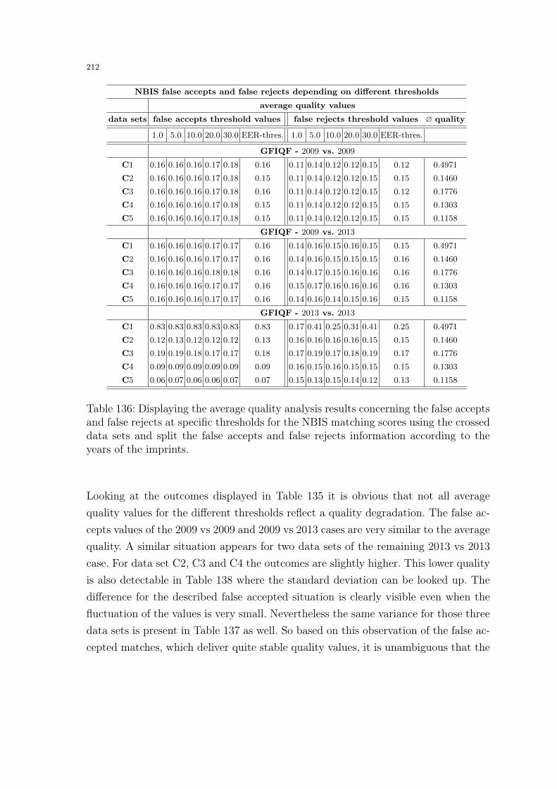
212





GFIQF - 2009 vs. 2009

C1 0.16 0.16 0.16 0.17 0.18 0.16 0.11 0.14 0.12 0.12 0.15 0.12 0.4971

C2 0.16 0.16 0.16 0.17 0.18 0.15 0.11 0.14 0.12 0.12 0.15 0.15 0.1460

C3 0.16 0.16 0.16 0.17 0.18 0.16 0.11 0.14 0.12 0.12 0.15 0.12 0.1776

C4 0.16 0.16 0.16 0.17 0.18 0.15 0.11 0.14 0.12 0.12 0.15 0.15 0.1303

C5 0.16 0.16 0.16 0.17 0.18 0.15 0.11 0.14 0.12 0.12 0.15 0.15 0.1158

GFIQF - 2009 vs. 2013

C1 0.16 0.16 0.16 0.17 0.17 0.16 0.14 0.16 0.15 0.16 0.15 0.15 0.4971

C2 0.16 0.16 0.16 0.17 0.17 0.16 0.14 0.16 0.15 0.15 0.15 0.16 0.1460

C3 0.16 0.16 0.16 0.18 0.18 0.16 0.14 0.17 0.15 0.16 0.16 0.16 0.1776

C4 0.16 0.16 0.16 0.17 0.17 0.16 0.15 0.17 0.16 0.16 0.16 0.16 0.1303

C5 0.16 0.16 0.16 0.17 0.17 0.16 0.14 0.16 0.14 0.15 0.16 0.15 0.1158

GFIQF - 2013 vs. 2013

C1 0.83 0.83 0.83 0.83 0.83 0.83 0.17 0.41 0.25 0.31 0.41 0.25 0.4971

C2 0.12 0.13 0.12 0.12 0.12 0.13 0.16 0.16 0.16 0.16 0.15 0.15 0.1460

C3 0.19 0.19 0.18 0.17 0.17 0.18 0.17 0.19 0.17 0.18 0.19 0.17 0.1776

C4 0.09 0.09 0.09 0.09 0.09 0.09 0.16 0.15 0.16 0.15 0.15 0.15 0.1303

C5 0.06 0.07 0.06 0.06 0.07 0.07 0.15 0.13 0.15 0.14 0.12 0.13 0.1158

Table 136: Displaying the average quality analysis results concerning the false acceptsand false rejects at specific thresholds for the NBIS matching scores using the crosseddata sets and split the false accepts and false rejects information according to theyears of the imprints.

Looking at the outcomes displayed in Table 135 it is obvious that not all averagequality values for the different thresholds reflect a quality degradation. The false ac-cepts values of the 2009 vs 2009 and 2009 vs 2013 cases are very similar to the averagequality. A similar situation appears for two data sets of the remaining 2013 vs 2013case. For data set C2, C3 and C4 the outcomes are slightly higher. This lower qualityis also detectable in Table 138 where the standard deviation can be looked up. Thedifference for the described false accepted situation is clearly visible even when thefluctuation of the values is very small. Nevertheless the same variance for those threedata sets is present in Table 137 as well. So based on this observation of the false ac-cepted matches, which deliver quite stable quality values, it is unambiguous that the

213

NBIS standard deviations (std)of the NFIQ quality analysis

data sets false accepts std false rejects std

A 0.20 1.31

B1 0.28 0.76

B2 0.32 1.48

B3 0.21 1.23

B4 0.13 0.93

B5 0.15 0.63

C1 0.19 0.56

C2 0.28 0.22

C3 0.33 0.17

C4 0.35 0.42

C5 0.12 0.57

Table 137: Displaying the standard deviations of the NFIQ quality analysis based onthe NBIS results.

NBIS standard deviations (std) ofthe NFIQ quality analysis for the splitted sets

data sets 2009 vs 2009 2009 vs 2013 2013 vs 2013

false accepted stds

C1 0.17 0.13 0.13

C2 0.22 0.24 0.19

C3 0.25 0.28 0.23

C4 0.15 0.18 0.15

C5 0.09 0.11 0.1

false rejected stds

C1 1.4 0.51 0.37

C2 1.04 0.20 0.44

C3 1.02 0.22 0.38

C4 1.09 0.29 0.54

C5 1.15 0.34 0.53

Table 138: Displaying the standard deviations of the NFIQ quality analysis based onthe NBIS results taking the time span information into account.

214

results of C2, C3 and C4 for the 2013 vs 2013 case are influencing the whole situationfor the entire NFIQ analysis of the NBIS fingerprint recognition system. Without therefinement it would not be possible to distinguish if the time span including matchesare responsible for the higher quality values or not.The same analysis as for the false accepts was performed for the crucial false rejectedmatches once more. Looking at the single values in Table 135 and at the standarddeviations in Table 137 and 138 it was possible to retrieve a very interesting infor-mation. Based on the results of the those tables two observation can be summarized.The first observation is based on the 2009 vs 2009 case. The matches, which are in-cluded in this class are mainly responsible for the poor average quality values whichhave been detected in Table 131. In Table 138 the standard deviation is confirmingthis situation. The second very important information is that the assumption thatquality is effecting the decrease of the EER and the genuine score shift, which aredetectable in the crossed data sets, can be disproved. The quality values for the timespan including 2009 vs 2013 case are not much higher as for the corresponding falseaccepted ones and the overall average of the entire data sets. Once more the consoli-dation of Table 138 confirms this aspect. Of course the standard deviation is a littlebit higher compared to the false accepted case, but not that high - for almost all datasets lower than 0.5. So it seems that for NBIS based on the NFIQ analysis it valid tostate that ageing is responsible for the detected effects in Chapter 5 and 6.

After discussing the NFIQ outcomes a detailed description of the derived IQF andGFIQF results is necessary. Especially interesting will be if there are also some dif-ferences detectable which improve the information obtained by the general qualityanalysis. Looking at the IQF results for the 2009 vs 2009 case it is observable that itseems that the differences between the quality values and the average quality valuesdisplayed in the last column are quite small. The only deviation is located in thequality values of the lowest threshold. Those entries are much higher compared tothe others and they also remain stable across all data sets. This observation is sharedwith the corresponding NFIQ measurements. Apart from this fluctuation, basicallya very small variation between the average and the other calculated threshold basedquality values appears for 2009 vs 2013 and 2013 vs 2013 outcomes as well. In fact inthe 2013 vs 2013 case there is some fluctuation in data set C1 which indicates that thefalse accepted matches tend to have a slightly worse quality. But even this deviation

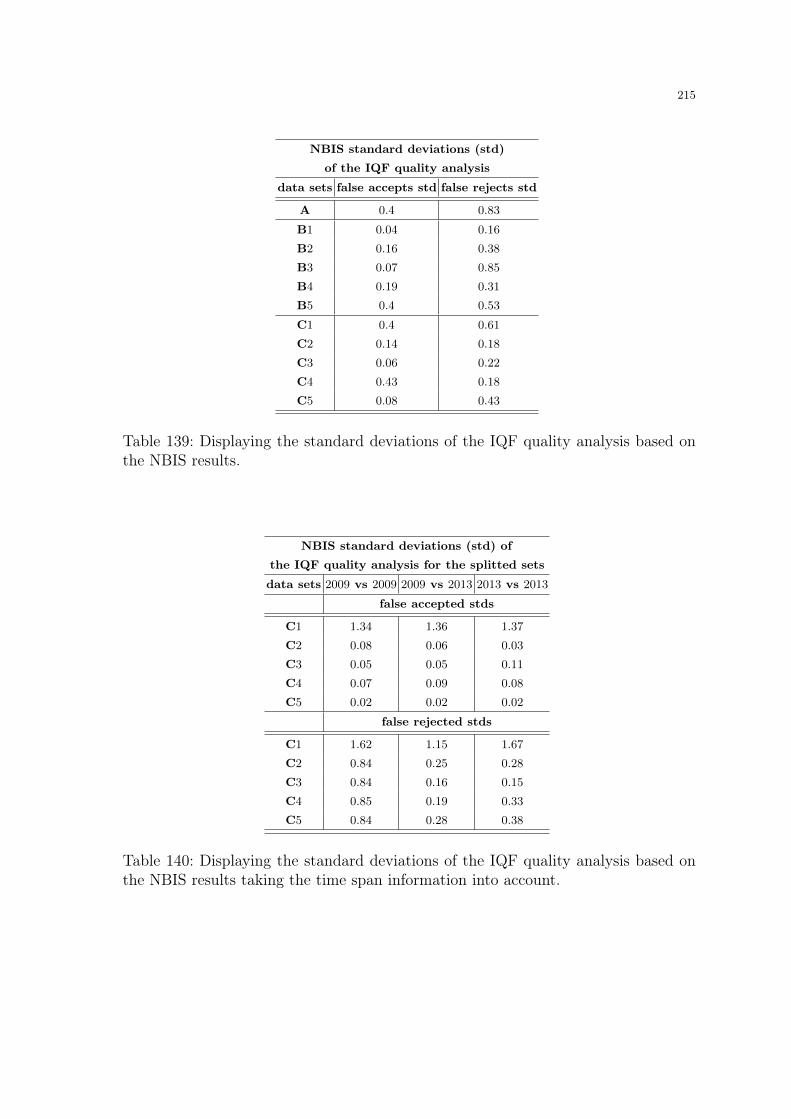
215

NBIS standard deviations (std)of the IQF quality analysis


A 0.4 0.83

B1 0.04 0.16

B2 0.16 0.38

B3 0.07 0.85

B4 0.19 0.31

B5 0.4 0.53

C1 0.4 0.61

C2 0.14 0.18

C3 0.06 0.22

C4 0.43 0.18

C5 0.08 0.43

Table 139: Displaying the standard deviations of the IQF quality analysis based onthe NBIS results.

NBIS standard deviations (std) ofthe IQF quality analysis for the splitted sets

data sets 2009 vs 2009 2009 vs 2013 2013 vs 2013

false accepted stds

C1 1.34 1.36 1.37

C2 0.08 0.06 0.03

C3 0.05 0.05 0.11

C4 0.07 0.09 0.08

C5 0.02 0.02 0.02

false rejected stds

C1 1.62 1.15 1.67

C2 0.84 0.25 0.28

C3 0.84 0.16 0.15

C4 0.85 0.19 0.33

C5 0.84 0.28 0.38

Table 140: Displaying the standard deviations of the IQF quality analysis based onthe NBIS results taking the time span information into account.

216

can not disprove the results from the general quality analysis like displayed in Table131 for the IQF measure. The corresponding quality values are more or less stableacross all data sets and performed matches. The standard deviations for the generalanalysis, displayed in Table 139, and for the splitted analysis, displayed in Table 140,are conforming to the situation as well. In fact it is also possible to detect in Table 140that for the false rejects the 2009 vs 2009 case there must be some higher deviationwithin as discussed before. The cross-sensor based effect for the data set includingthe imprints using the T2 sensor is also clearly visible for the standard deviations ofthe false accepted and rejected analysis. Concluding it can be said that for the NBISfingerprint recognition system using IQF no quality based impact can be observed.Therefore, as for the NFIQ analysis, the detected probably ageing effects must becaused by fingerprint ageing.Finally there will be a short discussion of the GFIQF quality refinement analysis. Thereason for this is basically the fact that looking at Table 136, 139 and 140 reveals moreor less the same situation which was described for the IQF analysis. There is hardlyno real difference detectable. The cross-sensor effect of data set C1 can be introducedas most interesting aspect in this case. So the GFIQF results are conforming the noquality based impact on the fingerprints and the clear existence of ageing.

In the following the results for the other fingerprint recognition system based on thequality refinement analysis will be presented. According to this at first the outcomesfor the second fingerprint recognition system using the minutiae concept were de-scribed. The results displayed in Table 143, 144, 147 and 148 were confirming all ofthe aspects detected for the NBIS fingerprint recognition system. In fact there weredifferent values and in case of the standard deviations a little bit more

fluctuations detectable.Those variations are in most of the cases lower than 0.5. Of course looking at theNFIQ outcomes the standard deviations are higher than 1.0 which indicates a quitehigh number of divergences but there is no doubt that the same tendency is present.Especially because those higher fluctuations are only present in the 2009 vs 2009 caseand for data set C1. So the time span and ageing including case is not influenced forthe remaining data sets using different sensor types. The cross-sensor related aspectof sensor T2 in data set C1 observed for IQF and GFIQF in the previous fingerprint

217

NBIS standard deviations (std)of the GFIQF quality analysis


A 0.11 0.04

B1 0.05 0.09

B2 0.03 0.03

B3 0.02 0.07

B4 0.02 0.06

B5 0.01 0.01

C1 0.03 0.22

C2 0.03 0.02

C3 0.03 0.02

C4 0.04 0.02

C5 0.06 0.02

Table 141: Displaying the standard deviations of the GFIQF quality analysis basedon the NBIS results.

NBIS standard deviations (std) ofthe GFIQF quality analysis for the splitted sets

data sets 2009 vs 2009 2009 vs 2013 2013 vs 2013

false accepted stds

C1 0.35 0.36 0.36

C2 0.02 0.02 0.01

C3 0.01 0.01 0.01

C4 0.04 0.03 0.03

C5 0.05 0.05 0.04

false rejected stds

C1 0.4 0.37 0.23

C2 0.02 0.01 0.01

C3 0.04 0.01 0.01

C4 0.01 0.03 0.03

C5 0.02 0.04 0.03

Table 142: Displaying the standard deviations of the GFIQF quality analysis basedon the NBIS results taking the time span information into account.

218





NFIQ - 2009 vs. 2009

C1 3.12 3.12 3.12 3.5 3.5 3.12 3.81 3.81 3.81 3.81 3.84 3.83 2.57

C2 3.12 3.12 3.12 3.5 3.5 3.12 3.81 3.81 3.81 3.81 3.84 3.83 2.92

C3 3.12 3.12 3.12 3.5 3.5 3.12 3.81 3.81 3.81 3.81 3.84 3.83 2.95

C4 3.12 3.12 3.12 3.5 3.5 3.12 3.81 3.81 3.81 3.81 3.84 3.83 2.86

C5 3.12 3.12 3.12 3.5 3.5 3.12 3.81 3.81 3.81 3.81 3.84 3.83 2.80

NFIQ - 2009 vs. 2013

C1 2.87 2.87 3.25 3.62 2.87 2.87 3.26 3.26 3.23 3.14 2.99 3.08 2.57

C2 2.94 2.94 2.89 3 2.94 2.94 3.14 3.14 3.12 3.04 2.91 2.94 2.92

C3 2.64 2.64 2.88 3.05 2.82 2.64 3.17 3.17 3.19 3.04 2.90 3.03 2.95

C4 2.62 2.62 2.75 3.12 2.62 2.62 3.31 3.31 3.31 3.24 3.10 3.27 2.86

C5 2.87 2.87 3.37 3.5 3 2.87 3.25 3.25 3.24 3.17 3.01 3.13 2.80

NFIQ - 2013 vs. 2013

C1 2.87 2.87 2.87 2.87 2.87 2.87 3.14 3.14 3.14 3.14 3.17 3.11 2.57

C2 3.21 3.21 3.31 3.31 3.21 3.21 3.26 3.26 3.26 3.23 3.27 3.12 2.92

C3 3.41 3.41 3.35 3.52 3.58 3.41 3.33 3.33 3.33 3.33 3.34 3.19 2.95

C4 2.7 2.7 3.1 3 2.6 2.7 3.4 3.4 3.4 3.38 3.38 3.31 2.86

C5 2.25 2.25 2.12 2.12 2.12 2.25 3.38 3.38 3.38 3.40 3.43 3.29 2.80

IQF - 2009 vs. 2009

C1 12.37 12.37 11.87 11.37 11.75 12.37 12.16 12.16 12.16 12.13 12 12.26 11.02

C2 12.37 12.37 11.87 11.37 11.75 12.37 12.16 12.16 12.16 12.13 12 12.26 12.32

C3 12.37 12.37 11.87 11.37 11.75 12.37 12.16 12.16 12.16 12.13 12 12.26 12.20

C4 12.37 12.37 11.87 11.37 11.75 12.37 12.16 12.16 12.16 12.13 12 12.26 12.18

C5 12.37 12.37 11.87 11.37 11.75 12.37 12.16 12.16 12.16 12.13 12 12.26 12.27

IQF - 2009 vs. 2013

C1 12.87 12.87 13 12.87 12.87 12.87 11.94 11.94 11.93 12.03 12.11 12.26 11.02

C2 12.68 12.68 12.94 12.89 12.68 12.68 12.08 12.08 12.09 12.20 12.23 12.13 12.32

C3 12.58 12.58 12.29 11.82 12.11 12.58 11.96 11.96 11.96 12.07 12.14 12.05 12.20

C4 12.87 12.87 12.75 13 12.87 12.87 11.97 12.97 12 12 12 11.97 12.18

C5 12.37 12.37 12.25 12.25 12.37 12.37 11.87 11.87 11.88 11.95 12.12 11.97 12.27

IQF - 2013 vs. 2013

C1 12.37 12.37 12.25 12.25 12.37 12.37 11.5 11.5 11.5 11.5 11.49 11.62 11.02

C2 12.73 12.73 12.73 12.73 12.73 12.73 12.15 12.15 12.15 12.15 12.04 12.20 12.32

C3 11.88 11.88 12.11 12.05 11.88 11.88 12.06 12.06 12.06 12.08 12.06 12 12.20

C4 12.1 12.1 12.2 12.5 12.2 12.1 11.95 11.95 11.94 11.93 11.91 11.96 12.18

C5 12.37 12.37 13.12 13.25 12.62 12.37 11.84 11.84 11.83 11.84 11.83 11.89 12.27

Table 143: Displaying the average quality analysis results concerning the false acceptsand false rejects at specific thresholds for the NEURO matching scores using thecrossed data sets and split the false accepts and false rejects information accordingto the years of the imprints.

219





GFIQF - 2009 vs. 2009

C1 0.18 0.18 0.17 0.05 0.18 0.18 0.09 0.09 0.09 0.1 0.1 0.1 0.4971

C2 0.18 0.18 0.17 0.05 0.18 0.18 0.09 0.09 0.09 0.1 0.1 0.1 0.1460

C3 0.18 0.18 0.17 0.05 0.18 0.18 0.09 0.09 0.09 0.1 0.1 0.1 0.1776

C4 0.18 0.18 0.17 0.05 0.18 0.18 0.09 0.09 0.09 0.1 0.1 0.1 0.1303

C5 0.18 0.18 0.17 0.05 0.18 0.18 0.09 0.09 0.09 0.1 0.1 0.1 0.1158

GFIQF - 2009 vs. 2013

C1 0.07 0.07 0.08 0.06 0.07 0.07 0.16 0.16 0.16 0.15 0.15 0.16 0.4971

C2 0.15 0.15 0.14 0.13 0.15 0.15 0.14 0.14 0.14 0.14 0.14 0.14 0.1460

C3 0.17 0.17 0.15 0.16 0.17 0.17 0.16 0.16 0.16 0.16 0.16 0.16 0.1776

C4 0.12 0.12 0.06 0.06 0.12 0.12 0.15 0.15 0.15 0.15 0.15 0.15 0.1303

C5 0.07 0.07 0.07 0.05 0.05 0.07 0.15 0.15 0.15 0.15 0.15 0.15 0.1158

GFIQF - 2013 vs. 2013

C1 0.41 0.41 0.41 0.41 0.41 0.41 0.3 0.3 0.3 0.31 0.31 0.28 0.4971

C2 0.08 0.08 0.09 0.09 0.08 0.08 0.15 0.15 0.15 0.15 0.15 0.15 0.1460

C3 0.14 0.14 0.14 0.08 0.10 0.14 0.2 0.2 0.2 0.2 0.19 0.19 0.1776

C4 0.13 0.13 0.22 0.23 0.13 0.13 0.16 0.16 0.16 0.16 0.16 0.16 0.1303

C5 0.16 0.16 0.29 0.41 0.29 0.16 0.13 0.13 0.14 0.14 0.14 0.14 0.1158

Table 144: Displaying the average quality analysis results concerning the false acceptsand false rejects at specific thresholds for the NEURO matching scores using thecrossed data sets and split the false accepts and false rejects information accordingto the years of the imprints.

recognition system analysis can be found once more as introduced. This time not onlyfor those two

quality methods rather for the NFIQ 2009 vs 20009 case as well. Another interestingobservation of the splitted quality analysis is the information that the results for thelowest threshold are not so different to the others. But it is clear that this effect inthe NBIS case was based on the choice of the certain value.The confirmation of ageing in the used fingerprint data sets with an time span of 4years for both minutiae based fingerprint recognition system seems to be a very solidfoundation to expect basically the same results for the upcoming refinement analysis

220

NEURO standard deviations (std)of the NFIQ quality analysis


A 1.49 1.23

B1 0.95 1.72

B2 0.83 1.41

B3 0.13 1.20

B4 0.51 1.41

B5 0.48 1.36

C1 1.28 0.58

C2 1.32 0.24

C3 0.14 0.29

C4 0.30 0.58

C5 0.13 0.50

Table 145: Displaying the standard deviations of the NFIQ quality analysis based onthe NEURO results.

NEURO standard deviations (std) ofthe NFIQ quality analysis for the splitted sets

data sets 2009 vs 2009 2009 vs 2013 2013 vs 2013

false accepted stds

C1 0.76 0.62 0.33

C2 0.41 0.04 0.36

C3 0.38 0.24 0.55

C4 0.46 0.24 0.21

C5 0.52 0.41 0.67

false rejected stds

C1 1.37 0.66 0.63

C2 0.98 0.17 0.35

C3 0.95 0.19 0.40

C4 1.05 0.44 0.57

C5 1.11 0.43 0.64

Table 146: Displaying the standard deviations of the NFIQ quality analysis based onthe NEURO results taking the time span information into account.

221

NEURO standard deviations (std)of the IQF quality analysis


A 2.07 0.11

B1 0.76 0.32

B2 0.63 0.35

B3 0.69 0.35

B4 0.58 0.2

B5 0.52 0.06

C1 1.32 0.63

C2 1.6 0.11

C3 0.27 0.04

C4 0.23 0.13

C5 0.55 0.22

Table 147: Displaying the standard deviations of the IQF quality analysis based onthe NEURO results.

NEURO standard deviations (std) ofthe IQF quality analysis for the splitted sets

data sets 2009 vs 2009 2009 vs 2013 2013 vs 2013

false accepted stds

C1 1.17 2.05 1.44

C2 0.53 0.5 0.45

C3 0.46 0.34 0.29

C4 0.45 0.76 0.15

C5 0.5 0.09 0.6

false rejected stds

C1 1.23 1.07 0.55

C2 0.2 0.2 0.19

C3 0.1 0.19 0.15

C4 0.09 0.2 0.25

C5 0.15 0.36 0.46

Table 148: Displaying the standard deviations of the IQF quality analysis based onthe NEURO results taking the time span information into account.

222

NEURO standard deviations (std)of the GFIQF quality analysis


A 0.09 0.06

B1 0.13 0.41

B2 0.01 0.02

B3 0.04 0.04

B4 0.05 0.08

B5 0.02 0.006

C1 0.27 0.22

C2 0.07 0.003

C3 0.04 0.003

C4 0.03 0.02

C5 0.1 0.02

Table 149: Displaying the standard deviations of the GFIQF quality analysis basedon the NEURO results.

NEURO standard deviations (std) ofthe GFIQF quality analysis for the splitted sets

data sets 2009 vs 2009 2009 vs 2013 2013 vs 2013

false accepted stds

C1 0.37 0.46 0.08

C2 0.05 0.009 0.06

C3 0.05 0.01 0.05

C4 0.06 0.04 0.06

C5 0.07 0.05 0.17

false rejected stds

C1 0.43 0.36 0.21

C2 0.05 0.001 0.008

C3 0.08 0.01 0.02

C4 0.03 0.02 0.04

C5 0.01 0.04 0.02

Table 150: Displaying the standard deviations of the GFIQF quality analysis basedon the NEURO results taking the time span information into account.

223





NFIQ - 2009 vs. 2009

C1 2.7 2.7 2.7 2.82 2.82 2.7 2.72 2.71 2.63 2.76 2.72 2.76 2.57

C2 2.7 2.7 2.7 2.81 2.81 2.69 2.71 2.71 2.66 2.71 2.71 2.76 2.92

C3 2.7 2.7 2.7 2.81 2.81 2.69 2.71 2.71 2.66 2.77 2.71 2.76 2.95

C4 2.74 2.74 2.74 2.85 2.85 2.74 2.71 2.71 2.66 2.77 2.71 2.75 2.86

C5 2.7 2.7 2.7 2.82 2.82 2.7 2.71 2.71 2.66 2.77 2.71 2.74 2.80

NFIQ - 2009 vs. 2013

C1 2.70 2.70 2.70 2.74 2.74 2.70 2.44 2.46 2.68 2.44 2.44 3.63 2.57

C2 2.70 2.70 2.70 2.74 2.74 2.69 3.12 3.15 2.92 3.13 3.13 3.19 2.92

C3 2.70 2.70 2.70 2.74 2.74 2.69 3.2 3.21 2.89 3.21 3.19 3.21 2.95

C4 2.70 2.70 2.70 2.74 2.74 2.70 3.01 3.06 2.92 3.02 3.01 3.01 2.86

C5 2.70 2.70 2.70 2.74 2.74 2.70 2.89 2.95 2.93 2.91 2.9 3 2.80

NFIQ - 2013 vs. 2013

C1 2.44 2.44 2.44 2.46 2.46 2.46 2.48 2.48 2.45 2.45 2.48 2.45 2.57

C2 3.13 3.13 3.13 3.04 3.03 3.13 3.14 3.41 3.16 3.29 3.14 3.19 2.92

C3 3.19 3.19 3.18 3.08 3.08 3.18 2.78 3.22 2.85 3.03 3.22 2.84 2.95

C4 3 3 3 2.92 2.91 2.98 2.95 2.96 3.05 3.06 2.95 3.07 2.86

C5 2.89 2.89 2.89 2.74 2.73 2.86 2.87 2.89 2.93 3 2.87 2.94 2.80

IQF - 2009 vs. 2009

C1 12.25 12.25 12.25 12.29 12.29 12.27 12.29 12.28 12.25 12.3 12.29 12.32 11.02

C2 12.25 12.25 12.25 12.30 12.30 12.30 12.28 12.26 11.98 12.31 12.29 12.28 12.32

C3 12.25 12.25 12.25 12.31 12.31 12.31 12.28 12.26 11.98 12.31 12.29 12.28 12.20

C4 12.21 12.21 12.21 12.27 12.27 12.25 12.28 12.26 11.98 12.31 12.29 12.28 12.18

C5 12.25 12.25 12.25 12.29 12.29 12.29 12.28 12.26 11.98 12.31 12.29 12.28 12.27

IQF - 2009 vs. 2013

C1 12.26 12.26 12.26 12.26 12.26 12.25 9.79 9.76 11.54 9.78 9.79 10.4 11.02

C2 12.26 12.26 12.26 12.26 12.26 12.25 12.39 12.39 11.98 12.39 12.39 12.39 12.32

C3 12.26 12.26 12.26 12.26 12.26 12.25 12.13 12.11 12.1 12.13 12.14 12.15 12.20

C4 12.26 12.26 12.26 12.26 12.26 12.25 12.1 12.08 12.08 12.1 12.1 12.09 12.18

C5 12.26 12.26 12.26 12.26 12.26 12.29 12.29 12.25 12.18 12.28 12.29 12.29 12.27

IQF - 2013 vs. 2013

C1 9.79 9.79 9.79 9.72 9.72 9.76 9.72 9.72 9.78 9.75 9.72 9.78 11.02

C2 12.37 12.37 12.37 12.31 12.31 12.34 12.38 12.38 12.38 12.31 12.38 12.35 12.32

C3 12.13 12.13 12.14 12.11 12.11 12.13 12.09 12.08 12.13 12.11 12.08 12.1 12.20

C4 12.08 12.08 12.09 12.04 12.05 12.07 12.09 12.09 12.09 12.07 12.09 12.13 12.18

C5 12.27 12.27 12.28 12.28 12.29 12.27 12.25 11.25 12.27 12.33 12.25 12.28 12.27

Table 151: Displaying the average quality analysis results concerning the false acceptsand false rejects at specific thresholds for the FC matching scores using the crosseddata sets and split the false accepts and false rejects information according to theyears of the imprints.

224





GFIQF - 2009 vs. 2009

C1 0.16 0.16 0.16 0.15 0.15 0.15 0.14 0.14 0.14 0.14 0.14 0.13 0.4971

C2 0.16 0.16 0.16 0.15 0.15 0.15 0.14 0.14 0.14 0.15 0.14 0.14 0.1460

C3 0.16 0.16 0.16 0.15 0.15 0.15 0.14 0.14 0.14 0.15 0.14 0.14 0.1776

C4 0.16 0.16 0.16 0.15 0.15 0.16 0.16 0.14 0.14 0.15 0.14 0.13 0.1303

C5 0.16 0.16 0.16 0.15 0.16 0.15 0.14 0.14 0.14 0.15 0.14 0.13 0.1158

GFIQF - 2009 vs. 2013

C1 0.16 0.16 0.16 0.15 0.15 0.15 0.82 0.82 0.82 0.82 0.83 0.62 0.4971

C2 0.16 0.16 0.16 0.15 0.15 0.16 0.12 0.12 0.13 0.12 0.12 0.11 0.1460

C3 0.16 0.16 0.16 0.15 0.15 0.16 0.19 0.18 0.15 0.19 0.19 0.17 0.1776

C4 0.16 0.16 0.16 0.15 0.15 0.16 0.09 0.1 0.13 0.09 0.09 0.13 0.1303

C5 0.16 0.16 0.16 0.15 0.15 0.16 0.06 0.06 0.13 0.06 0.06 0.07 0.1158

GFIQF - 2013 vs. 2013

C1 0.82 0.82 0.82 0.82 0.82 0.82 0.81 0.81 0.82 0.82 0.81 0.83 0.4971

C2 0.12 0.12 0.12 0.11 0.11 0.12 0.11 0.11 0.12 0.12 0.11 0.12 0.1460

C3 0.18 0.18 0.18 0.18 0.18 0.18 0.17 0.16 0.18 0.2 0.17 0.18 0.1776

C4 0.09 0.09 0.09 0.1 0.1 0.09 0.09 0.09 0.09 0.1 0.09 0.1 0.1303

C5 0.06 0.06 0.06 0.07 0.07 0.06 0.06 0.06 0.06 0.06 0.06 0.06 0.1158

Table 152: Displaying the average quality analysis results concerning the false acceptsand false rejects at specific thresholds for the FC matching scores using the crosseddata sets and split the false accepts and false rejects information according to theyears of the imprints.

of the non-minutiae fingerprint recognition system results.

The output of the quality refinement analysis using the FC fingerprint recognitionsystem can be read in Table 151, 152, 155 and 156. It is even harder to detect anydifferences in the non minutiae fingerprint recognition system results as for the minu-tiae fingerprint recognition system quality analysis variations. That means that firstof all the same overall tendency as for the previously discussed quality outcomes canbe detected. There are just two types of varieties. For the 2009 vs 2009 case there isno real discrepancy observable as before and the quality values seem to be more sim-ilar as for the minutiae based fingerprint recognition system. This stronger similarity

225

FC standard deviations (std)of the NFIQ quality analysis


A 0.32 0.14

B1 0.19 0.24

B2 0.51 0.98

B3 0.09 0.57

B4 0.46 0.65

B5 0.42 0.94

C1 0.19 0.57

C2 0.19 0.29

C3 0.04 0.28

C4 0.10 0.21

C5 0.11 0.25

Table 153: Displaying the standard deviations of the NFIQ quality analysis based onthe FC results.

FC standard deviations (std) ofthe NFIQ quality analysis for the splitted sets

data sets 2009 vs 2009 2009 vs 2013 2013 vs 2013

false accepted stds

C1 0.20 0.16 0.12

C2 0.20 0.22 0.20

C3 0.23 0.25 0.23

C4 0.10 0.15 0.13

C5 0.08 0.08 0.08

false rejected stds

C1 0.17 0.12 0.11

C2 0.21 0.23 0.29

C3 0.25 0.25 0.27

C4 0.15 0.16 0.17

C5 0.09 0.15 0.13

Table 154: Displaying the standard deviations of the NFIQ quality analysis based onthe FC results taking the time span information into account.

226

FC standard deviations (std)of the IQF quality analysis


A 0.35 1.90

B1 0.35 0.09

B2 1.97 0.85

B3 0.11 1.86

B4 0.4 0.48

B5 0.4 0.80

C1 0.59 0.96

C2 0.21 0.19

C3 0.06 0.3

C4 0.14 0.35

C5 0.05 0.37

Table 155: Displaying the standard deviations of the IQF quality analysis based onthe FC results.

FC standard deviations (std) ofthe IQF quality analysis for the splitted sets

data sets 2009 vs 2009 2009 vs 2013 2013 vs 2013

false accepted stds

C1 1.37 1.36 1.37

C2 0.04 0.06 0.04

C3 0.09 0.06 0.07

C4 0.07 0.09 0.11

C5 0.02 0.008 0.01

false rejected stds

C1 1.39 1.16 1.39

C2 0.15 0.08 0.06

C3 0.13 0.07 0.10

C4 0.14 0.09 0.09

C5 0.13 0.04 0.03

Table 156: Displaying the standard deviations of the IQF quality analysis based onthe FC results taking the time span information into account.

227

FC standard deviations (std)of the GFIQF quality analysis


A 0.37 0.06

B1 0.07 0.11

B2 0.02 0.03

B3 0.007 0.04

B4 0.03 0.02

B5 0.02 0.02

C1 0.04 0.09

C2 0.03 0.03

C3 0.09 0.09

C4 0.07 0.02

C5 0.06 0.02

Table 157: Displaying the standard deviations of the GFIQF quality analysis basedon the FC results.

FC standard deviations (std) ofthe GFIQF quality analysis for the splitted sets

data sets 2009 vs 2009 2009 vs 2013 2013 vs 2013

false accepted stds

C1 0.36 0.36 0.36

C2 0.01 0.01 0.02

C3 0.01 0.01 0.01

C4 0.03 0.03 0.03

C5 0.04 0.05 0.05

false rejected stds

C1 0.38 0.31 0.35

C2 0.004 0.02 0.03

C3 0.03 0.01 0.01

C4 0.01 0.03 0.03

C5 0.03 0.04 0.05

Table 158: Displaying the standard deviations of the GFIQF quality analysis basedon the FC results taking the time span information into account.

228





NFIQ - 2009 vs. 2009

C1 2.71 2.71 2.68 2.71 2.68 2.72 2.84 2.73 2.74 2.78 2.70 3.05 2.57

C2 2.71 2.71 2.68 2.71 2.68 2.72 - 3.04 2.78 2.73 2.74 2.79 2.92

C3 2.71 2.71 2.69 2.71 2.69 2.73 - 3.05 2.78 2.73 2.74 2.85 2.95

C4 2.71 2.71 2.68 2.71 2.68 2.72 - 3.04 2.78 2.73 2.74 2.82 2.86

C5 2.71 2.71 2.68 2.71 2.68 2.72 - 3.03 2.78 2.73 2.74 2.81 2.80

NFIQ - 2009 vs. 2013

C1 2.44 2.44 2.47 2.44 2.47 2.44 2.74 2.82 2.70 2.70 2.78 2.69 2.57

C2 3.13 3.13 3.13 3.13 3.13 3.13 - 2.96 2.72 2.70 2.70 2.80 2.92

C3 3.19 3.19 3.13 3.19 3.13 3.19 - 3.08 2.73 2.71 2.7 2.89 2.95

C4 3.01 3.01 2.97 3.02 2.97 3.01 - 3.13 2.77 2.71 2.71 2.89 2.86

C5 2.90 2.90 2.87 2.91 2.86 2.89 - 3.12 2.72 2.70 2.70 2.90 2.80

NFIQ - 2013 vs. 2013

C1 2.44 2.44 2.43 2.44 2.43 2.44 2.70 2.68 2.69 2.75 2.78 2.68 2.57

C2 3.12 3.10 3.10 3.09 3.10 3.06 - 2.74 2.96 3.01 3.12 2.73 2.92

C3 3.18 3.17 3.16 3.17 3.16 3.14 - 2.76 3.05 3.05 3.16 2.75 2.95

C4 3 2.99 2.98 2.99 2.98 2.96 - 2.76 2.89 2.88 2.96 2.75 2.86

C5 2.89 2.87 2.84 2.87 2.84 2.83 - 2.75 2.91 2.93 2.99 2.75 2.80

IQF - 2009 vs. 2009

C1 12.26 12.24 12.18 12.24 12.18 12.25 12.23 12.28 12.28 12.29 12.26 12.01 11.02

C2 12.26 12.24 12.18 12.24 12.18 12.26 - 12.06 12.29 12.28 12.28 12.26 12.32

C3 12.26 12.24 12.18 12.24 12.18 12.26 - 12.05 12.29 12.28 12.28 12.26 12.20

C4 12.26 12.24 12.18 12.24 12.18 12.25 - 12.06 12.29 12.28 12.28 12.25 12.18

C5 12.26 12.24 12.18 12.24 12.18 12.26 - 12.08 12.29 12.28 12.28 12.25 12.27

IQF - 2009 vs. 2013

C1 9.79 9.79 9.74 9.78 9.74 9.79 12.28 12.22 12.26 12.26 12.26 12.25 11.02

C2 12.26 12.24 12.18 12.24 12.18 12.26 - 12.16 12.26 12.26 12.26 12.27 12.32

C3 12.14 12.14 12.11 12.12 12.11 12.14 - 12.18 12.25 12.25 12.25 12.26 12.20

C4 12.26 12.24 12.18 12.24 12.18 12.10 - 12 12.23 12.26 12.27 12.16 12.18

C5 12.29 12.29 12.30 12.27 12.31 12.29 - 12.02 12.23 12.25 12.26 12.16 12.27

IQF - 2013 vs. 2013

C1 9.8 9.8 9.76 9.79 9.76 9.8 12.25 11.98 11 11.01 11.8 11.98 11.02

C2 12.38 12.38 12.39 12.38 12.39 12.36 - 12.23 12.19 12.15 12.14 12.23 12.32

C3 12.13 12.11 12.10 12.11 12.10 12.11 - 12.26 12.24 12.19 12.13 12.23 12.20

C4 12.10 12.09 12.10 12.08 12.10 12.06 - 12.25 12.13 12.14 12.13 12.25 12.18

C5 12.29 12.3 12.28 12.3 12.29 12.29 - 12.17 12.13 12.19 12.16 12.18 12.27

Table 159: Displaying the average quality analysis results concerning the false acceptsand false rejects at specific thresholds for the POC matching scores using the crosseddata sets and split the false accepts and false rejects information according to theyears of the imprints.

229





GFIQF - 2009 vs. 2009

C1 0.16 0.16 0.16 0.16 0.16 0.16 0.14 0.16 0.16 0.15 0.16 0.13 0.4971

C2 0.16 0.16 0.16 0.16 0.16 0.15 - 0.15 0.15 0.16 0.16 0.14 0.1460

C3 0.16 0.16 0.16 0.16 0.16 0.15 - 0.15 0.15 0.16 0.16 0.14 0.1776

C4 0.16 0.16 0.16 0.16 0.16 0.15 - 0.15 0.15 0.16 0.16 0.14 0.1303

C5 0.16 0.16 0.16 0.16 0.16 0.15 - 0.15 0.15 0.16 0.16 0.14 0.1158

GFIQF - 2009 vs. 2013

C1 0.83 0.83 0.85 0.83 0.85 0.83 0.16 0.16 0.15 0.16 0.16 0.16 0.4971

C2 0.12 0.12 0.13 0.12 0.13 0.12 - 0.16 0.16 0.16 0.16 0.16 0.1460

C3 0.19 0.19 0.18 0.18 0.18 0.19 - 0.16 0.16 0.16 0.16 0.17 0.1776

C4 0.09 0.09 0.10 0.09 0.10 0.09 - 0.14 0.16 0.16 0.16 0.15 0.1303

C5 0.06 0.06 0.07 0.06 0.07 0.06 - 0.16 0.16 0.16 0.16 0.16 0.1158

GFIQF - 2013 vs. 2013

C1 0.83 0.83 0.85 0.83 0.85 0.83 0.16 0.22 0.47 0.47 0.52 0.22 0.4971

C2 0.12 0.13 0.13 0.13 0.13 0.12 - 0.16 0.15 0.15 0.15 0.16 0.1460

C3 0.19 0.19 0.18 0.18 0.18 0.18 - 0.17 0.20 0.20 0.19 0.17 0.1776

C4 0.09 0.10 0.10 0.10 0.10 0.09 - 0.16 0.17 0.16 0.15 0.16 0.1303

C5 0.07 0.07 0.07 0.07 0.07 0.07 - 0.15 0.13 0.13 0.11 0.15 0.1158

Table 160: Displaying the average quality analysis results concerning the false acceptsand false rejects at specific thresholds for the POC matching scores using the crosseddata sets and split the false accepts and false rejects information according to theyears of the imprints.

could be described for the entire data sets the first time and the refinement analysisis conforming this tendency. Therefore the standard deviation values are much lowerthan 0.5. In fact they are never higher than 0.3. The only exception is the 2009 vs2009 case.Based on the FC results it is easy to analyze the outcomes of the POC refinementresearch. As readable in Table 159, 160, 163 and 164 just one disparity between thenon minutiae based fingerprint recognition system is observable. This difference isthat there are other output values of the calculations. The standard deviations arenever higher than 0.3 and most of the time they are lower than for all the otherfingerprint recognition systems. Of course the cross-sensor effect is the exception for

230

POC standard deviations (std)of the NFIQ quality analysis


A 1.23 0.11

B1 0.27 0.5

B2 1.02 0.24

B3 0.19 0.41

B4 0.53 0.62

B5 0.55 0.57

C1 0.11 0.15

C2 0.34 0.08

C3 0.33 0.07

C4 0.13 0.07

C5 0.21 0.09

Table 161: Displaying the standard deviations of the NFIQ quality analysis based onthe POC results.

POC standard deviations (std) ofthe NFIQ quality analysis for the splitted sets

data sets 2009 vs 2009 2009 vs 2013 2013 vs 2013

false accepted stds

C1 0.15 0.12 0.14

C2 0.23 0.23 0.19

C3 0.26 0.25 0.24

C4 0.16 0.15 0.13

C5 0.10 0.10 0.07

false rejected stds

C1 0.12 0.18 0.16

C2 0.16 0.18 0.17

C3 0.18 0.21 0.18

C4 0.13 0.17 0.08

C5 0.12 0.18 0.13

Table 162: Displaying the standard deviations of the NFIQ quality analysis based onthe POC results taking the time span information into account.

231

POC standard deviations (std)of the IQF quality analysis


A 1.12 0.08

B1 0.21 0.39

B2 0.68 0.09

B3 0.57 0.14

B4 0.5 0.11

B5 0.39 0.21

C1 0.35 0.86

C2 0.16 0.06

C3 0.19 0.06

C4 0.09 0.05

C5 0.2 0.08

Table 163: Displaying the standard deviations of the IQF quality analysis based onthe POC results.

POC standard deviations (std) ofthe IQF quality analysis for the splitted sets

data sets 2009 vs 2009 2009 vs 2013 2013 vs 2013

false accepted stds

C1 1.32 1.36 1.34

C2 0.1 0.06 0.07

C3 0.04 0.07 0.09

C4 0.06 0.1 0.09

C5 0.05 0.03 0.02

false rejected stds

C1 1.32 1.35 0.82

C2 0.13 0.09 0.14

C3 0.1 0.06 0.05

C4 0.11 0.11 0.06

C5 0.09 0.13 0.11

Table 164: Displaying the standard deviations of the IQF quality analysis based onthe POC results taking the time span information into account.

232

POC standard deviations (std)of the GFIQF quality analysis


A 0.08 0.01

B1 0.11 0.13

B2 0.04 0.03

B3 0.06 0.04

B4 0.02 0.01

B5 0.01 0.01

C1 0.1 0.3

C2 0.03 0.01

C3 0.03 0.002

C4 0.03 0.02

C5 0.03 0.03

Table 165: Displaying the standard deviations of the GFIQF quality analysis basedon the POC results.

POC standard deviations (std) ofthe GFIQF quality analysis for the splitted sets

data sets 2009 vs 2009 2009 vs 2013 2013 vs 2013

false accepted stds

C1 0.36 0.37 0.36

C2 0.01 0.01 0.01

C3 0.01 0.01 0.01

C4 0.03 0.03 0.03

C5 0.05 0.05 0.04

false rejected stds

C1 0.37 0.36 0.22

C2 0.01 0.01 0.01

C3 0.02 0.01 0.02

C4 0.03 0.03 0.03

C5 0.05 0.05 0.03

Table 166: Displaying the standard deviations of the GFIQF quality analysis basedon the POC results taking the time span information into account.

233

this statement like before.

As last part of the present Chapter 7 it is necessary to summarize the informationwhich has been discussed. Especially the aspect of quality and ageing in terms of thedetected effects of the previous chapters will be in the main focus.In Section 7.1 the NFIQ quality measure was introduced. The results of the calcu-lations using this method are located between 1 and 5. It is easy to understand themeaning of those values. 1 denotes the best possible quality and 5 the worst. The ideaof using a low number for better quality is not repeated for the other two methods.For IQF and GFIQF a low output indicates worse and a high one good quality of thefingerprint image. In Section 7.2 the range of IQF is introduced to be between 0 and100. But this range was never covered of one of the used data bases. All quality valuesof the present fingerprints are always lower than 20 which is a reference for a quitebad quality at all. This assumption was confirmed by the other two measurements.Particularly the range of GFIQF, which was described in Section 7.3 the first time,supported the outcomes of IQF mainly. The GFIQF values are located between 0

and 1 and for the most of the fingerprint images in the present data sets they neverexceeded 0.2. This is interesting because both methods are using a total differentconcept. The NFIQ measure was the only one for which the whole range was coveredby the imprints. Based on this information it is probably valid to state that the NFIQmeasure is the most important one of those three quality measurements because theoutcomes can describe the actual quality of the fingerprints in a more sophisticatedway.Another aspect that is very important to discuss is the circumstance if it is realis-tic that ageing is influencing the matching performance so much that false positivematches occur. Those type of matches would be included in the impostor matches.If the number of those falsely accepted matches would be influenced by ageing thatmuch, this could lead to a lot of troubles in terms of security aspects. But what doesthis potential high degradation of the fingerprints mean? In fact there would be apart of the human population for whom the persistence aspect of their imprints wouldnot be given. Their fingerprints could chance that much that they would get a newbiometric identification feature. That would imply that there are people having thepotential to be a kind of ’human chameleons’. So far as it is known this would violatea lot of laws of nature - especially thinking about the generally accepted concept of

234

DNA as main genetic code book for development and reproduction of cells. Thereforethe results displayed in Chapter 5 based on the stability of the impostor score distri-butions is a result which seems to be realistic to detect. Based on the stability of theimpostor score distribution it is also not surprising that there is hardly no qualitybased impact detectable in the present Chapter 7 concerning the quality analysis ofthe used fingerprints.A slightly different point of view is necessary for the genuine score distribution andthe corresponding quality analysis. Because of the aspect mentioned above ageingcan only cause some troubles in terms of convenience. In the quality analysis of thischapter it was possible to gather the information that the average quality of theentire data sets and the quality based on certain thresholds and matching classes(2009 vs 2009, 2009 vs 2013, 2013 vs 2013) is very similar. Various variations whichhave been discussed using the standard deviation are not influencing the aspect thatquality degradation is not present in the false rejected matches. So the quality of thefalsely rejected matches is also not better or worse than the average quality of thecomplete data bases. Because of the clearly observable decrease of the EER for thecrossed data sets it is valid to say that this effect is caused by ageing. The assurancethat ageing is the reason therefore is ensured by the stability of the quality values. Ifthis stability would not be present a total different situation could be described. Anincrease or decrease concerning the quality of the false rejected matches could only becaused by quality itself. Otherwise ageing would violate the persistence characteristicof biometric features like discussed above.So based on the quality investigations which have been presented in this chapter ofthe current master thesis the assumption that ageing is causing the detected effectsof the previous chapters can be confirmed.

235

8 Conclusion

Three main goals have been stated in the introduction of this master thesis. In thisfinal section of the thesis there will be a closing discussion to summarize the beforepresented results. On a CASIA fingerprint data base, including imprints, which havebeen acquired with a time interval of four years, the experiments, examining the ma-jor tasks, are performed.As described in Chapter 3 four fingerprint recognition systems are employed on thedata sets to derive the matching performance. For this purpose the results, describedin Chapter 5, revealed that the characteristic values of each data base and systemtype can be used to observe some interesting effects. In fact there are irregularitiesconcerning the matching score distributions detectable. The clearly present shift tothe left in the genuine score distributions of the crossed data bases leaded to the hy-pothesis that ageing is influencing the number of falsely rejected matches. This shiftis also indicating that the number of low genuine scores is increased. Furthermore itcan be stated that the genuine and impostor score distributions for the crossed dataset tend to be more similar as for the single data sets. The security based point ofview of this statement can be discussed as well. The increase of false rejected matchesis not a big problem in terms of security, but in convenience. In terms of security theresults revealed that nearly no change in the impostor score distribution is detectableand also not in the number of false accepted users. Despite it is important to addthe information that within the calculated matching scores of the crossed data sets itseems that it does not matter which type of impostor matches are taken into account.As discussed in WA, OA and HH analysis of Chapter 5 using different score subsetsof the entire crossed matching scores there is hardly no difference between the 3 cho-sen experimental setups. Furthermore a randomly performed adaptation of the usedscores’ size during the experiments did not change the results either. Neverthelessafter performing the first main task of the master thesis it was not possible to besure that ageing is responsible for the observed effects. It was a regular assumptionthat fingerprint quality and ageing as well could cause the discussed aspects. For thispurpose a more detailed study on this topic was performed in the last Chapter 7.Looking at the outcomes of the experiments displayed in Section 3 it is possible toreceive a different point of view in terms of fingerprint ageing using the so called’Doddington’s Zoo’ concept. Especially the goats characteristic is interesting because

236

they are related to low genuine scores and as discussed before an irregularity concern-ing the genuine scores is observable within the crossed data. As described in Chapter6 some experiments have been performed to get a closer look at the menagerie in-vestigation. The intuition would probably lead to the suggestion that an increase oflow genuine scores must also give rise to the number of detectable goat-like user’s.But against this proposition nearly no difference between the number of goat labeleduser’s in the used data can be proven. It seems that the number is more or less sta-ble. Of course it is a little bit difficult to state data set specific results because ofthe structure of the used method to find certain users. For the mean, var, mean2and min/max a fixed number of volunteers is labeled for each data base. So the onlyaspect which can be compared is based on all data set information. That means thatall volunteers of 2013 and of the crossed sets have been taken into account. So it ispossible to gather a total number of all users, which have been labeled in 2009, 2013and the crossed data bases. These sets of volunteers are compared for each data set.In particular it can be stated that if a volunteer has been labeled in 2009 or 2013

the first time then the probability to sign the same user in the crossed sets can belocated between at least 30% and 40%. An additional assumption that the decreasewithin the genuine scores and the stability of the impostor scores is influencing theoverall observation could not be confirmed. Contrary to what was expected there wasno high amount of fluctuation/stability in the extension of the users’ goats/lambsand wolves characteristic detectable. For both goats and lambs/wolves a more or lessidentical likelihood of resigning a volunteer in the crossed data sets can be described.Of course there are differences which are caused by the variances in data bases, recog-nition system and menagerie analysis method. But a more detailed discussion waspresented in Chapter 6.6.The final main goal of this master thesis was to determine the impact of the finger-print quality. It is clear that the quality of the imprints is a very crucial key aspect.There is no doubt, bad quality of imprints can lead to several troubles performing afingerprint recognition. So it also is possible that quality which is bad enough and hasa much higher impact as ageing effects. For this purpose a very detailed discussionhas been performed about this topic. It was possible to get the information that notquality is responsible for the before discussed effects in terms of performance andmenagerie analysis. Fingerprint ageing is detectable in the data sets and this bio-logical aspect is also more influencing the described experiments than quality. Apart

237

form the results it is possible to state the following general assumption: If bad qualityis detectable then it could be that the effects detected in the before mentioned ex-perimental setups are caused by low quality and not because of ageing. But, if thereis hardly no quality based bias then for example the trend of the genuine score dis-tributions adaptation of the impostor ones for the crossed data sets would be causedby fingerprint ageing. After the quality based investigations it was clear that thereare more or less no quality based aspects for the time span including matches de-tectable. So the observed effects of the other main parts of the present master thesisare caused by fingerprint ageing itself. Furthermore it is also important to mentionthat there are false rejected matches which correspond to imprints from 2009 andfor whom an quality bias is verifiable. But those matches are not responsible for thetime span based effects and due to this their quality degradation is not important forthis study. Apart from this the false accepted matches seem to be not influenced byquality at all. This observation is a realistic one because otherwise there could be aproblem in terms of fingerprint recognition security which would refer to a weaknessin the concepts of biometric persistence and uniqueness.All in all it is possible to reveal ageing effects in fingerprint recognition in the usedexperimental setups and data bases. It would be interesting to have a closer look atother data sets on the one hand and especially on data sets including a larger timespan. A more detailed look at the genuine score distributions could be also very in-formative due to more concrete convenience aspects. In terms of the very importantquality analysis the application of further quality measures, for example NFIQ 2.0,to separate the gray area between ageing effects and quality into more detail wouldbe an interesting task. Even though it seems that the quality aspect in the used dataset is not biasing the ageing related matches in a strong manner.

238

References

1. "Fingerprint Verification Competition 2004", http://bias.csr.unibo.it/fvc2004/, [Online; last ac-cess 17.July 2015]

2. National Institute of Standards and Technology: User’s Guide to the NIST Biometric Image Software,http://www.nist.gov/customcf/get_pdf.cfm?pub_id=51097, [Online; last access 17.July 2015]

3. NIST Biometric Image Software package: National Institute for Standards and Technologie, http:

//www.nist.gov/itl/iad/ig/nbis.cfm, [Online; last access 17.July 2015]4. "VeriFinger SDK 7.1" - Algorithmic Information, Neurotechnology, Lithuania, http://www.

neurotechnology.com/verifinger-technology.html#algorithm, [Online; last access 17.July 2015]5. "VeriFinger SDK 7.1" - General Information, Neurotechnology, Lithuania, http://www.

neurotechnology.com/verifinger.html, [Online; last access 17.July 2015]6. Alonso-Fernandez, F., Fierrez, J., Ortega-Garcia, J., Gonzalez-Rodriguez, J., Fronthaler, H., Kollreider,

K., Bigun, J.: A comparative study of fingerprint image-quality estimation methods. Information Foren-sics and Security, IEEE Transactions on 2(4), 734–743 (2007), http://www.diva-portal.org/smash/get/diva2:239227/FULLTEXT01.pdf, [Online; last access 22.July 2015]

7. Alonso Fernández, F., Veldhuis, R., Bazen, A.M., Fiérrez, J., Ortega-Garcia, J.: On the relation betweenbiometric quality and user-dependent score distributions in fingerprint verification. Proc. of Workshopon Multimodal User Authentication - MMUA (2006), http://mmua.cs.ucsb.edu/MMUA2006/Papers/141.pdf, [Online; last access 22.July 2015]

8. Ashbourne, J.: Biometrics: Advanced Identification Technology. Springer (2000), http://www.springer.com/?SGWID=4-102-45-130566-p2275653, [Online; last access 17.July 2015]

9. Barnes, J.G.: The Fingerprint Sourcebook. National Institute of Justice (2010), https://www.ncjrs.gov/pdffiles1/nij/225320.pdf, [Online; last access 17.July 2015]

10. Bevilacqua, A., Gherardi, A.: Age-related skin analysis by capacitance images. In: Pattern Recognition,2004. ICPR 2004. Proceedings of the 17th International Conference on. vol. 2, pp. 703–706. IEEE(2004), http://www.researchgate.net/profile/Alessandro_Bevilacqua/publication/220927478_

Age-related_Skin_Analysis_by_Capacitance_Images/links/00b4951616312368cf000000.pdf, [On-line; last access 20.July 2015]

11. Bolle, R., Connell, J.H., Pankanti, S., Ratha, N.K., Senior, A.W.: Guide to Biometrics. Springer NewYork (2004)

12. Doddington, G., Liggett, W., Martin, A., Przybocki, M., Reynolds, D.: Sheep, Goats, Lambs andWolves:A statistical analysis of speaker performance in the NIST 1998 speaker recognition evaluation. In: ICSLP1998. Proceedings of the 5th International Conference on Spoken Language Processing. vol. 4, pp.1351–1354. ICSLP (1998), http://www.itl.nist.gov/iad/mig/publications/storage_paper/icslp_98.pdf, [Online; last access 17.July 2015]

13. Dollé, M.E., Snyder, W.K., Dunson, D.B., Vijg, J.: Mutational fingerprints of aging. Nucleic acidsresearch 30(2), 545–549 (2002), http://nar.oxfordjournals.org/content/30/2/545.long, [Online;last access 20.July 2015]

14. Fairhurst, M.: Age factors in biometric processing. Institution of Engineering and Technology (2013)15. Galton, F.: Fingerprints. Macmillan and Co. (1892), http://galton.org/books/finger-prints/

galton-1892-fingerprints-1up.pdf, [Online; last access 17.July 2015]16. Gopi, K., Pramod, J.: Fingerprint recognition using gabor filter and frequency domain filtering. Jour-

nal of Electronics and Communication Engineering 2(6), 17–21 (2012), http://iosrjournals.org/iosr-jece/papers/vol2-issue6/E0261721.pdf, [Online; last access 20.July 2015]

http://bias.csr.unibo.it/fvc2004/

http://www.nist.gov/customcf/get_pdf.cfm?pub_id=51097

http://www.nist.gov/itl/iad/ig/nbis.cfm

http://www.nist.gov/itl/iad/ig/nbis.cfm

http://www.neurotechnology.com/verifinger-technology.html#algorithm

http://www.neurotechnology.com/verifinger-technology.html#algorithm

http://www.neurotechnology.com/verifinger.html

http://www.neurotechnology.com/verifinger.html

http://www.diva-portal.org/smash/get/diva2:239227/FULLTEXT01.pdf

http://www.diva-portal.org/smash/get/diva2:239227/FULLTEXT01.pdf

http://mmua.cs.ucsb.edu/MMUA2006/Papers/141.pdf

http://mmua.cs.ucsb.edu/MMUA2006/Papers/141.pdf

http://www.springer.com/?SGWID=4-102-45-130566-p2275653

http://www.springer.com/?SGWID=4-102-45-130566-p2275653

https://www.ncjrs.gov/pdffiles1/nij/225320.pdf

https://www.ncjrs.gov/pdffiles1/nij/225320.pdf

http://www.researchgate.net/profile/Alessandro_Bevilacqua/publication/220927478_Age-related_Skin_Analysis_by_Capacitance_Images/links/00b4951616312368cf000000.pdf

http://www.researchgate.net/profile/Alessandro_Bevilacqua/publication/220927478_Age-related_Skin_Analysis_by_Capacitance_Images/links/00b4951616312368cf000000.pdf

http://www.itl.nist.gov/iad/mig/publications/storage_paper/icslp_98.pdf

http://www.itl.nist.gov/iad/mig/publications/storage_paper/icslp_98.pdf

http://nar.oxfordjournals.org/content/30/2/545.long

http://galton.org/books/finger-prints/galton-1892-fingerprints-1up.pdf

http://galton.org/books/finger-prints/galton-1892-fingerprints-1up.pdf

http://iosrjournals.org/iosr-jece/papers/vol2-issue6/E0261721.pdf

http://iosrjournals.org/iosr-jece/papers/vol2-issue6/E0261721.pdf

239

17. Hämmerle-Uhl, J., Pober, M., Uhl, A.: Towards standardised fingerprint matching robustness assess-ment: the stirmark toolkit–cross-database comparisons with minutiae-based matching. In: Proceedingsof the first ACM workshop on Information hiding and multimedia security. pp. 111–116. ACM (2013)

18. Ito, K., Morita, A., Aoki, T., Nakajima, H., Kobayashi, K., Higuchi, T.: A fingerprint recognition algo-rithm combining phase-based image matching and feature-based matching. In: Advances in Biometrics,pp. 316–325. Springer (2005), http://www.aoki.ecei.tohoku.ac.jp/research/docs/316.pdf, [Online;last access 20.July 2015]

19. Jain, A., Ross, A., Prabhakar, S.: Fingerprint matching using minutiae and texture features. In: ImageProcessing, 2001. Proceedings. 2001 International Conference on. vol. 3, pp. 282–285. IEEE (2001),http://citeseerx.ist.psu.edu/viewdoc/download?doi=10.1.1.33.88&rep=rep1&type=pdf, [Online;last access 20.July 2015]

20. Jain, A.K., Ross, A., Prabhakar, S.: An introduction to biometric recognition. Circuits and Systems forVideo Technology, IEEE Transactions on 14(1), 4–20 (2004), http://www2.cse.msu.edu/~rossarun/BiometricsTextBook/Papers/Introduction/JainRossPrabhakar_BiometricIntro_CSVT04.pdf, [On-line; last access 20.July 2015]

21. Kukula, E., Elliott, S., Kim, H., Martin, C.S.: The impact of fingerprint force on image qualityand the detection of minutiae. In: Electro/Information Technology, 2007 IEEE International Con-ference on. pp. 432–437. IEEE (2007), http://icbrpurdue.org/wp-content/uploads/2014/01/

2007-The-Impact-of-Fingerprint-Force-on-Image-Quality-and-Detection-of-Minutiae.pdf,[Online; last access 22.July 2015]

22. Lanitis, A., Tsapatsoulis, N., Maronidis, A.: Review of ageing with respect to biometrics and diversemodalities. Age Factors in Biometric Processing (2013)

23. Maltoni, D., Maio, D., Jain, A.K., Prabhakar, S.: Handbook of Fingerprint Recognition. Springer Science& Business Media (2009)

24. Modi, S.K., Elliott, S.J., Whetsone, J., Kim, H.: Impact of age groups on fingerprint recognition per-formance. In: Automatic Identification Advanced Technologies, 2007 IEEE Workshop on. pp. 19–23.IEEE (2007), http://perso.telecom-paristech.fr/~chollet/Biblio/Articles/Domaines/BIOMET/

RASC/229_quality.pdf, [Online; last access 20.July 2015]25. Nakajima, H., Kobayashi, K., Higuchi, T.: A fingerprint matching algorithm using phase-only cor-

relation. IEICE Transactions on Fundamentals of Electronics, Communications and Computer Sci-ences 87(3), 682–691 (2004), http://dhoto.lecturer.pens.ac.id/publications/conference/2004/1-IES2004-ucc-surabaya/e87-a_3_682.pdf, [Online; last access 20.July 2015]

26. Nill, N.B.: IQF (Image Quality of Fingerprint) software application. The MITRE Corporation (2007),http://www.mitre.org/sites/default/files/pdf/07_0580.pdf, [Online; last access 22.July 2015]

27. Pankanti, S., Prabhakar, S., Jain, A.K.: On the individuality of fingerprints. Pattern Analysis andMachine Intelligence, IEEE Transactions on 24(8), 1010–1025 (2002), http://www.researchgate.

net/profile/S_Pankanti/publication/3193438_On_the_individuality_of_fingerprints/links/

0912f50ecd7b62205b000000.pdf, [Online; last access 20.July 2015]28. Petrovska-Delacrétaz, D., Chollet, G., Dorizzi, B.: Guide to biometric reference systems and performance

evaluation. Springer (2009)29. Reedman, C.: Fingerprints and human inspection: a forensics perspective. Age Factors in Biometric

Processing p. 221 (2013)30. Ross, A., Jain, A., Reisman, J.: A hybrid fingerprint matcher. Pattern Recognition 36(7), 1661–1673

(2003), http://www2.cse.msu.edu/~rossarun/pubs/RossHybrid_PR03.pdf, [Online; last access 18.July2015]

http://www.aoki.ecei.tohoku.ac.jp/research/docs/316.pdf

http://citeseerx.ist.psu.edu/viewdoc/download?doi=10.1.1.33.88&rep=rep1&type=pdf

http://www2.cse.msu.edu/~rossarun/BiometricsTextBook/Papers/Introduction/JainRossPrabhakar_BiometricIntro_CSVT04.pdf

http://www2.cse.msu.edu/~rossarun/BiometricsTextBook/Papers/Introduction/JainRossPrabhakar_BiometricIntro_CSVT04.pdf

http://icbrpurdue.org/wp-content/uploads/2014/01/2007-The-Impact-of-Fingerprint-Force-on-Image-Quality-and-Detection-of-Minutiae.pdf

http://icbrpurdue.org/wp-content/uploads/2014/01/2007-The-Impact-of-Fingerprint-Force-on-Image-Quality-and-Detection-of-Minutiae.pdf

http://perso.telecom-paristech.fr/~chollet/Biblio/Articles/Domaines/BIOMET/RASC/229_quality.pdf

http://perso.telecom-paristech.fr/~chollet/Biblio/Articles/Domaines/BIOMET/RASC/229_quality.pdf

http://dhoto.lecturer.pens.ac.id/publications/conference/2004/1-IES2004-ucc-surabaya/e87-a_3_682.pdf

http://dhoto.lecturer.pens.ac.id/publications/conference/2004/1-IES2004-ucc-surabaya/e87-a_3_682.pdf

http://www.mitre.org/sites/default/files/pdf/07_0580.pdf

http://www.researchgate.net/profile/S_Pankanti/publication/3193438_On_the_individuality_of_fingerprints/links/0912f50ecd7b62205b000000.pdf



http://www2.cse.msu.edu/~rossarun/pubs/RossHybrid_PR03.pdf

240

31. Ross, A., Rattani, A., Tistarelli, M.: Exploiting the doddington zoo effect in biometric fusion. In:Biometrics: Theory, Applications, and Systems, 2009. BTAS’09. IEEE 3rd International Confer-ence on. pp. 1–7. IEEE (2009), http://www2.cse.msu.edu/~rossarun/pubs/RossRattaniTistarelli_DoddingtonBTAS2009.pdf, [Online; last access 18.July 2015]

32. Ross, A., Reisman, J., Jain, A.: Fingerprint matching using feature space correlation. In: Bio-metric Authentication, pp. 48–57. Springer (2002), http://www2.cse.msu.edu/~rossarun/pubs/

RossCorrelation_ECCV02.pdf, [Online; last access 18.July 2015]33. Severance, C.: Anil jain: 25 years of biometric recognition. Computer 48(8), 8–10 (2015)34. Shen, L., Kot, A., Koo, W.: Quality measures of fingerprint images. In: Audio-and Video-based Biomet-

ric Person Authentication. pp. 266–271. Springer (2001), http://citeseerx.ist.psu.edu/viewdoc/download?doi=10.1.1.61.5682&rep=rep1&type=pdf, [Online; last access 22.July 2015]

35. Sickler, N.C., Elliott, S.J.: An evaluation of fingerprint image quality across an elderly populationvis-a-vis an 18-25 year old population. In: Security Technology, 2005. CCST’05. 39th Annual 2005International Carnahan Conference on. pp. 68–73. IEEE (2005)

36. Tabassi, E., Wilson, C., Watson, C.: Nist fingerprint image quality. NIST Res. Rep. NIS-TIR7151 http://biometrics.nist.gov/cs_links/standard/archived/workshops/workshop1/

presentations/Tabassi-Image-Quality.pdf, [Online; last access 20.July 2015]37. Uhl, A., Wild, P.: Comparing verification performance of kids and adults for fingerprint, palmprint,

hand-geometry and digitprint biometrics. In: Biometrics: Theory, Applications, and Systems, 2009.BTAS’09. IEEE 3rd International Conference on. pp. 1–6. IEEE (2009), http://wavelab.at/papers/Uhl09c.pdf, [Online; last access 20.July 2015]

38. Uhl, A., Wild, P.: Experimental evidence of ageing in hand biometrics. In: Biometrics Special InterestGroup (BIOSIG), 2013 International Conference of the. pp. 1–6. IEEE (2013), http://cs.emis.de/LNI/Proceedings/Proceedings212/39.pdf, [Online; last access 20.July 2015]

39. Watson, C., Garris, M., Tabassi, E., Wilson, C., Janet, S., Ko, K.: User’s Guide to Export ControlledDistribution of NIST Biometric Image Software (NBIS-EC) http://citeseerx.ist.psu.edu/viewdoc/download?doi=10.1.1.152.7979&rep=rep1&type=pdf, [Online; last access 18.July 2015]

40. Yager, N., Dunstone, T.: The biometric menagerie. Pattern Analysis and Machine Intelligence, IEEETransactions on 32(2), 220–230 (2010)

41. Yoon, S., Jain, A.K.: Longitudinal study of fingerprint recognition. Proceedings of the National Academyof Sciences of the United States of America (PNAS) 112(28), 8555–8560 (2015), http://www.pnas.org/content/112/28/8555.full.pdf?sid=e4724717-3305-4f86-9d79-81f69a920f7d, [Online; last access16.September 2015]

42. Zhao, D., Su, F., Cai, A.: A hierarchical fingerprint matching method based on rotation in-variant features. In: Advances in Biometric Person Authentication. pp. 498–505. Springer(2005), http://bupt-mcprl.net/admin/newessay/A%20Hierarchical%20Fingerprint%20Matching%

20Method%20Based%20on%20Rotation%20Invariant%20Features.pdf, [Online; last access 20.July 2015]

http://www2.cse.msu.edu/~rossarun/pubs/RossRattaniTistarelli_DoddingtonBTAS2009.pdf

http://www2.cse.msu.edu/~rossarun/pubs/RossRattaniTistarelli_DoddingtonBTAS2009.pdf

http://www2.cse.msu.edu/~rossarun/pubs/RossCorrelation_ECCV02.pdf

http://www2.cse.msu.edu/~rossarun/pubs/RossCorrelation_ECCV02.pdf



http://biometrics.nist.gov/cs_links/standard/archived/workshops/workshop1/presentations/Tabassi-Image-Quality.pdf

http://biometrics.nist.gov/cs_links/standard/archived/workshops/workshop1/presentations/Tabassi-Image-Quality.pdf

http://wavelab.at/papers/Uhl09c.pdf

http://wavelab.at/papers/Uhl09c.pdf

http://cs.emis.de/LNI/Proceedings/Proceedings212/39.pdf

http://cs.emis.de/LNI/Proceedings/Proceedings212/39.pdf



http://www.pnas.org/content/112/28/8555.full.pdf?sid=e4724717-3305-4f86-9d79-81f69a920f7d

http://www.pnas.org/content/112/28/8555.full.pdf?sid=e4724717-3305-4f86-9d79-81f69a920f7d

http://bupt-mcprl.net/admin/newessay/A%20Hierarchical%20Fingerprint%20Matching%20Method%20Based%20on%20Rotation%20Invariant%20Features.pdf

http://bupt-mcprl.net/admin/newessay/A%20Hierarchical%20Fingerprint%20Matching%20Method%20Based%20on%20Rotation%20Invariant%20Features.pdf

ageing effects in fingerprint recognition

Documents