Sensors 2007, 7, 1359-1386

sensors ISSN 1424-8220 © 2007 by MDPI

http://www.mdpi.org/sensors

Full Paper

Agent Collaborative Target Localization and Classification in Wireless Sensor Networks

Xue Wang *, Dao-wei Bi † , Liang Ding ‡ and Sheng Wang §

State Key Laboratory of Precision Measurement Technology and Instrument, Tsinghua University,

Beijing 100084, P. R. China; E-mails: † bdw02@mails.tsinghua.edu.cn; ‡dintliang03@mails.tsinghua.edu.cn ; §wang_sheng00@mails.tsinghua.edu.cn

* Author to whom correspondence should be addressed; E-mail: wangxue@mail.tsinghua.edu.cn

Received: 26 June 2007 / Accepted: 27 July 2007 / Published: 30 July 2007

Abstract: Wireless sensor networks (WSNs) are autonomous networks that have been

frequently deployed to collaboratively perform target localization and classification tasks.

Their autonomous and collaborative features resemble the characteristics of agents. Such

similarities inspire the development of heterogeneous agent architecture for WSN in this

paper. The proposed agent architecture views WSN as multi-agent systems and mobile

agents are employed to reduce in-network communication. According to the architecture,

an energy based acoustic localization algorithm is proposed. In localization, estimate of

target location is obtained by steepest descent search. The search algorithm adapts to

measurement environments by dynamically adjusting its termination condition. With the

agent architecture, target classification is accomplished by distributed support vector

machine (SVM). Mobile agents are employed for feature extraction and distributed SVM

learning to reduce communication load. Desirable learning performance is guaranteed by

combining support vectors and convex hull vectors. Fusion algorithms are designed to

merge SVM classification decisions made from various modalities. Real world experiments

with MICAz sensor nodes are conducted for vehicle localization and classification.

Experimental results show the proposed agent architecture remarkably facilitates WSN

designs and algorithm implementation. The localization and classification algorithms also

prove to be accurate and energy efficient.

Keywords: wireless sensor networks, multi-agent system, mobile agent, target localization

and classification, support vector machine.

Sensors 2007, 7

1360

1. Introduction

Wireless sensor networks (WSNs) are wireless networks that consist of a large number of spatially

distributed autonomous sensors (generally referred to as sensor nodes) and collectively monitor

environmental conditions, such as temperature, sound, vibration, and so forth [1,2]. WSN can be

employed in applications ranging from environmental monitoring and battlefield surveillance to

condition based maintenance [1,2,3]. Among the tasks of these applications, target localization and

classification are most frequently involved [3,4,5,6,7]. Both tasks can be viewed as sensor fusion

problems as illustrated in [2]. More specifically, the target localization and classification problem is to

make the best estimates with regard to the location and type of the observed targets by rationally

combining information collected by relevant sensor nodes [2].

A thorough overview of these problems can be found in [3]. In the publication, a general purpose

collaborative framework is proposed for localization and classification in WSN. Localization problems

are overviewed in [4,5,6]. It shows localization is primarily achieved by two approaches, i.e. by

estimate of time delay of arrival (TDOA) or estimate of energy attenuation. Each algorithm has its own

advantages and disadvantages [6]. In [3] energy based localization using acoustic signatures in WSN

is presented. Classification in WSN is reported in [3,7]. In [3], maximum likelihood and support vector

machine are used for classification. Real world experiments to classify armed vehicles with acoustic

and seismic signatures are demonstrated in [7].

In WSN scenarios, the energy based localization method is preferred. The primary reason is that

TDOA requires related sensors to be accurately synchronized. But accurate synchronization at present

is too expensive. Localization with acoustic signatures is most desirable, because the models of

acoustic energy attenuation are relatively easy to establish and less influenced by environmental

changes. Support vector machine [7] is very suitable for classification in WSN because it is especially

designed for small sample learning. Moreover its sparse representation of the learned classifier requires

less in-network data exchange.

As shown in [2], localization and classification in WSN are in essence sensor fusion problems. It

necessitates cooperation between sensor nodes and collaborative processing algorithms. The

collaboration entails in-network information exchanges, but in WSN limited bandwidth and power

supply make bulk data exchanges prohibitively expensive [1,3].

To deal with the above problems, a variety of energy efficient collaborative processing algorithms

have been developed [3,8,9,10,11]. An information-driven collaborative algorithm is introduced in [9].

Different from the method in [9], mobile agents are employed to perform collaborative processing in

WSN in [10,11]. Mobile agents can remarkably reduce in-network wireless transmission by migrating

in the network to perform assigned tasks [10,11]. The characteristics of agents (including mobile

agents and multi-agents) such as autonomy, reactivity, and social ability perfectly match the

autonomous, reactive and collaborative features of WSN [10,12]. Such resemblance has motivated

attempts to model WSN as a multi-agent system as reported in [13,14].

Undoubtedly it is desirable to use these proposed architectures to develop scalable WSN systems.

But in literatures [10,12] only mobile agents are exploited, while in literatures [13,14] merely multi-

agents are investigated. Intuitively the potentials of agents will be better exploited if multi-agents and

Sensors 2007, 7

1361

mobile agents are merged. Inspired by this, we propose to model WSN with a heterogeneous agent

system (i.e. a combination of mobile agents and multi-agents). It is believed such architecture

represents WSN better than solely using either of them.

The proposed architecture is a hierarchical one. The entire WSN is viewed as a multi-agent system.

Individual agents belong to different hierarchical levels in accordance with their roles in the network.

Collaborative processing (or equivalently, sensor fusion) is primarily accomplished by multi-agent

cooperation, but mobile agents are also used in cases of bulk data exchanges. This architecture greatly

facilitates designs and implementations of WSN. In addition the architecture also readily adapts to

diversified deployments at various scales.

With the agent architecture, target localization and classification in WSN are implemented

accordingly. Energy based acoustic localization is achieved by multi-agent collaboration. An adaptive

steepest descent search algorithm is introduced to search for the best estimate of target location. Target

classification is achieved by a combination of multi-agent and mobile agent using SVM. Distributed

SVM learning using convex hull vectors is developed to enhance the learning accuracy with low

communication needs. Acoustic and seismic signatures are observed for classification’s purpose. The

features are extracted by means of wavelet packet decomposition. Fusion algorithms are devised to

merge classification decisions made by agents using features of different modalities.

Experiments are conducted to evaluate the proposed architecture and corresponding collaborative

algorithms. Results show that the proposed architecture remarkably facilitates the system designs and

implementations. Applications of vehicle localization and classification show the proposed steepest

descent search and distributed SVM algorithms are energy efficient and accurate.

The rest of the paper is organized as follows. In section 2, existent agent architectures for WSN are

introduced. Existent algorithms for target localization and classification are overviewed in section 3. In

the section that follows, the heterogeneous agent architecture is developed. Agent collaborative

algorithms for localization and classification are accordingly proposed respectively. In section 5 real

world experiments of vehicle localization and classification are conducted and the results are reported.

A conclusion is given in section 6.

2. Existent Agent Architectures for Wireless Sensor Networks

2.1. Brief overview of multi-agent systems and mobile agents

The terms multi-agent and mobile agent have long been used in research communities, however

paradoxically they are effectively not clearly defined [12]. To make them fit into the objectives in this

paper, the definition of agent given in [12] is adopted. According to [12], agent is defined as “a

computational mechanism that exhibits a high degree of autonomy, performing actions in its

environment based on information (sensors, feedback) received from the environment”.

A multi-agent system is one where there is more than one agent, and where the agents interact with

one another [12]. For WSN applications, hierarchical multi-agent systems are of particular interests.

Here hierarchy is used in the sense system components from different task levels are represented by

different agents. Such systems have significant implications for WSN, as is to be illustrated soon.

Sensors 2007, 7

1362

In contrast, a mobile agent can be regarded as a special kind of agent which has the unique feature

of mobility [10]. A mobile agent migrates from one sensor node to another to autonomously perform

assigned tasks. Usually the derived results are sent back to the sensor node that dispatches the mobile

agent, but the mobile agent itself generally destructs locally.

Note that a sensor node is an autonomous entity which makes decisions by reasoning with the

information acquired by its sensors [2]. Evidently the characteristics of a sensor node match the agent

definition perfectly. The sensor node, therefore, can be viewed as an agent. Consequently it would be

appropriate to model WSN in software with multi-agent systems and mobile agents.

2.2. Multi-agent and mobile agent architectures for wireless sensor networks

Now that a sensor node can be viewed as an agent, it is straightforward to consider WSN as a multi-

agent system. The hierarchical multi-agent architecture is presented for WSN in [14]. Mobile agents

have been found wide application in WSN too.

The multi-agent architecture in [14] is briefly summarized as follows. The entire WSN is viewed as

a homogeneous hierarchical multi-agent system. The top agent is the interface agent. It is responsible

for accepting user requests, processing them and providing feedbacks. It also dispatches instructions to

agents at lower levels. Based on geographical conditions and other factors, WSN can be divided into

regions managed by regional agents. A region is further split into several sub-regions called clusters

and managed by cluster agents. At the bottom of the hierarchy is the query agent, which actually

corresponds to a sensor node.

Apparently the established hierarchical agent architecture is an adequate software abstraction of the

functionalities of WSN. But it is more than a simple software model. Its cooperative, social and

adaptive characteristics make designs and implementations of scalable WSN much easier.

Applications of mobile agents in WSN is mainly driven by some drawbacks of the prevalent

client/server computing paradigms [10,11] .Collaborative computing paradigms with mobile agents

have been proposed to address these drawbacks. In such paradigms, instead of sending raw data from

sensor nodes to the server, mobile agents carrying processing codes are sent to these sensor nodes to

carry out local processing. When local processing is finished, derived results are sent back. Usually the

size of the codes carried by a mobile agent is much smaller compared to the data to be sent.

Accordingly communication energy consumption is drastically reduced.

Compared to multi-agent architectures for WSN, mobile agent architectures are relatively simple

and straightforward. In such architectures, mobile agents are usually dispatched by a sink node or base

station and migrate from one sensor node to another to perform assigned tasks. Since the mobile agents

are essentially software codes, they can be dynamically programmed. Therefore the architectures offer

much flexibility to collaboration processing in WSN and make the network adaptive to various types of

applications. As stated above, multi-agent and mobile agent architectures for WSN make it easier to

design the network structures and implement collaborative processing algorithms between sensor

nodes. It is also clear that these two architectures are essentially complementary. If they are combined,

their strengths will be fully exploited. Later in the paper, a merged architecture will be proposed and

applied to collaborative localization and classification in WSN.

Sensors 2007, 7

1363

Before a merged architecture and its applications are investigated, the problems of localization and

classification are overviewed first to prepare the background for further discussion.

3. Target Localization and Classification Algorithms

In this section, several localization and classification algorithms are briefly presented. Signatures of

a variety of modalities can be used for target localization in WSN [5,9,15]. But acoustic signatures are

most frequently used because such signatures can be easily measured and the localization accuracy is

good [3,4,6]. Thus the discussion is confined to acoustic localization. Contrast to localization,

classification relies less on signature modalities; therefore it is discussed in a general sense.

3.1. Target localization with acoustic signatures

3.1.1 Propagation of acoustic signatures

In the paper, the localization problem is constrained within two dimensions, that is, the target is assumed to be positioned in a plane. Suppose the acoustic signature emitted by the target at position sp

is ( )su t and it propagates at the velocity ofc . In cases where the acoustic wave propagates in the air, the

velocity c can be assumed to be a constant of 340m/s. Two dimensional propagation of the acoustic

signature is mathematically represented by [3,6]:

1

( ) ( )4r s sr

s r

u t u t tπ

= −−p p

(1)

where ( )ru t is the acoustic signature propagated to location rp whose Cartesian coordinates are

expressed by

[ , ]T

r r rx y=p (2)

Note 1

sr s rt c−= −p p (3)

is the time needed for the signature to travel from location sp to rp . ⋅ represents the vector 2-norm:

2 2[ , ]Tx y x y= + (4)

Suppose a microphone sensor m is deployed at positionmp and the sensor gain ismα . Then the

acoustic signature measured by the sensor is [6]

( ) ( ) ( )4

mm s sm m

s m

u t u t t n tα

π= − +

−p p (5)

Sensors 2007, 7

1364

where ( )mn t is additive noise (assumed to be uncorrelated with the source signature).

Eq.(5) is a comprehensive description of the propagating characteristics of acoustic signatures.

Information of the acoustic source can be inferred from this equation. Specifically the acoustic localization problem is to estimate sp from the observed signature( )mu t by the microphone sensor. The

algorithms to be introduced rely heavily on the above propagation models, especially Eq. (5).

3.1.2 TDOA method

Acoustic signature reaches deployed sensors at different time. The term smt in Eq.(5) exactly

describes such time delay of arrival (TDOA). Though the absolute TDOA can not be measured without knowledge of locationsp , the relative TDOA mrt of sensor m at mp with respect to reference sensor r

at rp can be determined by means of cross correlation [6, 16]

,arg max ( )mr r mt R τ = (6)

,

1( ) ( ) ( )

T

r m r mR u t u t dtT τ

τ ττ

= −− ∫ (7)

Note , ( )r mR τ is the cross correlation of ( )mu t and ( )ru t . Recall from Eq.(3) mrt is determined by

( )1mr sm sr s m s rt t t c−= − = − − −p p p p (8)

In Eq.(8), there are two unknowns (note [ , ]T

s s sx y=p ), therefore another such equation is needed to

determine sp . If another sensor n positioned at np is available, then we have

s m s r mr

s n s r nr

t c

t c

− − − =

− − − =

p p p p

p p p p (9)

Solution of Eq.(9) yields the estimated position *

sp of the target whose true location issp . In its

formulation TDOA is involved. That is why this approach is called TDOA method.

3.1.3 Energy based method

When an acoustic signature is propagating, it essentially propagating energy emitted from the source.

Physically, energy of vibration is proportional to the square of vibration amplitude. Following Eq.(1),

energy decays in a manner that is inversely proportional to the square of the distance from the source

[4]:

2s

m

s m

k EE

⋅=

−p p (10)

where k is a coefficient, sE is the source energy at sP and mE is the energy propagated tomP .

Sensors 2007, 7

1365

Similar to the principles of TDOA method, though absolute energy can not be measured, relative energy mrE can be calculated:

' 2

2 '

' 2

2 '

1( )

1( )

T T

mTm

mr T T

rTr

u t dt

Eu t dt

α

α

+

+=

∫

∫ (11)

On the other hand, using Eq.(10) mrE is determined by

2

2s rm

mrr s m

EE

E

−= =

−

p p

p p (12)

Following the same principle of the solution in the TDOA method, the target position can be

estimated by combining several equations similar to Eq.(12). Evidently it is called energy based

method because energy propagation models play the dominant role in the formulation of this algorithm.

Observe the similarities between the TDOA method and energy based method. They both estimate

the true target position by inferring from known relative quantities (relative time delay and energy

respectively). Comparatively, the former method is less affected by noises as a result of cross

correlation but requires more computation (evaluation of Eq.(6) necessitates investigation of a large

number of possibleτ ) . Moreover it requires accurate synchronization of the involved sensors. The

latter is relatively efficient in computation but vulnerable to noises. Choosing the appropriate

localization method is problem specific where tradeoff between accuracy and efficiency may be needed.

3.2. Target classification with support vector machine

In the context of this paper, target classification is to infer which hypothesis the target belongs to

from the signatures observed by deployed sensors. Classification algorithms have been extensively

investigated [3,7,17]; therefore there are a rich set of algorithms for choice. In WSN scenarios, support

vector machine (SVM) [17,18,19] is especially applicable and suitable, for available samples come in

small number due to limited memory. Another appealing merit of SVM is its sparseness. By sparseness,

it means the learned SVM classifier is represented by only a small portion of given samples in most

cases. In other words, support vector machine implicitly performs data compression. Such data

compression makes SVM extremely suitable for WSN applications, because it can significantly reduce

communication load. Classification in WSN is essentially distributed due to the distributed sensor

deployment. Consequently distributed SVM learning schemes need to be exploited.

3.2.1 Fundamentals of support vector machine

Mathematically a binary classification problem is formulated as [17,18]: given a set of N samples

1{( , )} Ni i ix y = where d

i ∈ ⊂x X R , { 1, 1}iy ∈ = + −Y and iy denotes the class label of the sampleix ,

Sensors 2007, 7

1366

determine the hypothesis ( , ) { ( , )}H H∈0x u x u that meets certain criteria. As far as SVM is concerned,

the criteria is minimization of structural risks and the hypothesis takes the following form [17]

{ }( , , ) | ( ( )) 0H b bφ= ⋅ + =x w x w x (13)

where :φ →X F maps elements in X to a higher dimensional feature space F ; w is the weight vector

and b is the bias. The notation( )⋅ denotes the inner product operator.

The hypothesis ( , , )H bx w minimizing structural risks is denoted by* ( , , )H bx w , which is determined

by the following quadric optimization [17,18]:

1 1 1

1max ( , )

2

N N N

i i j i j i ji i j

y y Kα

α α α= = =

−∑ ∑∑ x x (14)

s.t. 1

0N

i ii

yα=

=∑ (15)

0 , 1, ,i C i Nα≤ ≤ = L (16)

In these equations, C is the predefined cost parameters. iα is the Lagrange multiplier.( )K ⋅ is a

kernel function defined as( , ) ( ( ) ( ))i j i jK φ φ= ⋅x x x x .

Suppose the optimal solution to Eq. (14) is* * * *1 2[ , ,..., ]Nα α α=α . Then jx associated with * 0jα ≠ is

called a support vector (SV). That is exactly why this method is named support vector machine. Let iSVdenotes the set{ }*| 0jj α ≠ . Then the derived hypothesis* ( , , )H bx w is expressed as [17]

* *( , , ) ( , )

i

m m mm SV

H b y K bα∈

= +∑x w x x (17)

Consequently, the decision function of SVM is [18]

*( ) sgn( ( , ) )m m m

m iSV

f y K bα∈

= +∑x x x (18)

The decision function (18) is based on the derived hypothesis (17), so the notations are identical with those used in (17). The sgn( )⋅ function is the sign function. Therefore (18) means that given any

new samplex , if * ( , ) 0m m mm iSV

y K bα∈

+ >∑ x x , then x belongs to class1+ (the output ofsgn( )⋅ ), otherwise 1− .

Note that the SVM classifier (17) is learned in a centralized manner, that is, all the samples are

available during the learning processing (i.e. solution of Eq.(14)). But in WSN, samples are distributed

over the network; consequently distributed learning methods need to be investigated.

Sensors 2007, 7

1367

3.2.2 Simple algorithm for distributed support vector machine learning

In WSN scenarios, the samples 1{( , )} Ni i ix y = are distributed across the network. Suppose the whole

samples (denoted byD ) are distributed over p sensors in WSN. The sample segment of D at the sensor k is denoted by kD . Distributed SVM learning from (1 )kD k p≤ ≤ can be transformed into a centralized

one, if all segments are sent to a concentration point where SVM is learned following Eq.(14) . But

such data concentration is not applicable in most WSN applications. As illustrated before, in WSN

bulk data transmission is prohibitive due to energy and bandwidth limitations. As a result, centralized

SVM learning is not feasible; therefore distributed learning needs to be exploited.

A simple distributed learning method is based upon the sparseness of SVM [19]. Note in Eq.(17),

only support vectors contribute to the final classifier. Moreover these support vectors usually account

for a small portion of the whole samples. In other words a SVM classifier is sparsely but sufficiently

represented by its support vectors. Based upon this observation, it is both intuitive and natural to

propose to learn the global SVM classifier from the concentration of local support vectors instead of local samples (1 )kD k p≤ ≤ . For detailed information concerning this method, please refer to [20]. In

this way, communication energy consumption is significantly decreased, because the numbers of

support vectors are much smaller compared to the whole samples. This simple intuitive learning

method is called ‘SV only’ algorithm because only local support vectors need to be transmitted for

final SVM learning.

3.2.3 Convex hull vector approach for distributed support vector machine learning

The SV only algorithm is very intuitive and indeed effective in some cases, but not in all cases. The

rationale of the SV only algorithm is that local support vectors are representative of local segments,

whose union is accordingly representative of the whole samples too. However this is not the truth.

There is a gap in between. In [21] convex hull is employed to draw representative samples from local

segments. The drawn samples are called hull vectors (HV) and their union is also representative of the

whole samples. The principle of convex hull is very straightforward and derived from observations that

in the feature space support vectors are always on the boundary of samples. This is shown in Figure 1.

In this figure diamonds and stars represent samples of two classes. The support vectors are

circumscribed by circles which are shown to be exactly on the boundaries. The boundary polygons are

called convex hulls and the samples on the polygons are the corresponding hull vectors.

An appealing characteristic of convex hull is that the convex hull of a large dataset can be

constructed with the convex hulls of its subsets. Therefore by convex hull, more information pertinent

to the local segments is preserved than the SV only algorithm. It is shown in [20] that compared to the

SV only algorithm, better distributed learning accuracy is achieved by using hull vectors in the feature

space to represent the local samples.

Sensors 2007, 7

1368

Figure 1. Convex hulls of samples in the feature space for SVM.

Figure 2. Divide and conquer algorithm to compute the convex hull (in 2-dimensions).

Determine hull(S), the convex hull of a point set S whose cardinality is n.

Step 1. If n≤2, then return the points, as they are the convex hull of S. Otherwise, perform the

remaining steps:

Step 2. Divide the n points by x-coordinate into 2 sets, A and B, each of size n/2, where all points in

A are to the left of all points in B.

Step 3. Recursively compute hull (A) and hull (B).

Step 4. Combine hull(A) and hull(B) to determine hull(S)=hull(hull(A)∪hull(B))

a) Find the upper and lower common tangent lines between hull (A) and hull (B). b) Discard the points in the quadrilateral formed by the 4 points that represent the tangent lines.

c) Number the convex points (i.e., enumerate the outermost points so that they remain ordered for

subsequent iterations).

A comprehensive introduction to convex hulls and algorithms to compute them can be found in [22].

Here a divide and conquer algorithm (in 2-dimensions) is presented and shown in Figure 2. The

algorithm is essentially a recursive one which is easy to understand and implement. However it must be

emphasized that convex hull computation in the feature space is very difficult. It requires explicit

mapping from the sample space to the feature space, which is at least presently a challenging problem.

Obviously for SV only and convex hull approaches, the former is simpler but the latter is more

accurate. Choice between the two algorithms depends on the objective of the distributed learning.

In the following section, the heterogeneous agent architecture is first developed; then the previously

discussed localization and classification algorithms are adapted for the proposed architecture.

Sensors 2007, 7

1369

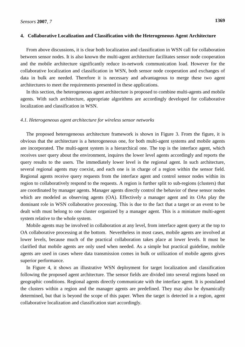
4. Collaborative Localization and Classification with the Heterogeneous Agent Architecture

From above discussions, it is clear both localization and classification in WSN call for collaboration

between sensor nodes. It is also known the multi-agent architecture facilitates sensor node cooperation

and the mobile architecture significantly reduce in-network communication load. However for the

collaborative localization and classification in WSN, both sensor node cooperation and exchanges of

data in bulk are needed. Therefore it is necessary and advantageous to merge these two agent

architectures to meet the requirements presented in these applications.

In this section, the heterogeneous agent architecture is proposed to combine multi-agents and mobile

agents. With such architecture, appropriate algorithms are accordingly developed for collaborative

localization and classification in WSN.

4.1. Heterogeneous agent architecture for wireless sensor networks

The proposed heterogeneous architecture framework is shown in Figure 3. From the figure, it is

obvious that the architecture is a heterogeneous one, for both multi-agent systems and mobile agents

are incorporated. The multi-agent system is a hierarchical one. The top is the interface agent, which

receives user query about the environment, inquires the lower level agents accordingly and reports the

query results to the users. The immediately lower level is the regional agent. In such architecture,

several regional agents may coexist, and each one is in charge of a region within the sensor field.

Regional agents receive query requests from the interface agent and control sensor nodes within its

region to collaboratively respond to the requests. A region is further split to sub-regions (clusters) that

are coordinated by manager agents. Manager agents directly control the behavior of these sensor nodes

which are modeled as observing agents (OA). Effectively a manager agent and its OAs play the

dominant role in WSN collaborative processing. This is due to the fact that a target or an event to be

dealt with must belong to one cluster organized by a manager agent. This is a miniature multi-agent

system relative to the whole system.

Mobile agents may be involved in collaboration at any level, from interface agent query at the top to

OA collaborative processing at the bottom. Nevertheless in most cases, mobile agents are involved at

lower levels, because much of the practical collaboration takes place at lower levels. It must be

clarified that mobile agents are only used when needed. As a simple but practical guideline, mobile

agents are used in cases where data transmission comes in bulk or utilization of mobile agents gives

superior performance.

In Figure 4, it shows an illustrative WSN deployment for target localization and classification

following the proposed agent architecture. The sensor fields are divided into several regions based on

geographic conditions. Regional agents directly communicate with the interface agent. It is postulated

the clusters within a region and the manager agents are predefined. They may also be dynamically

determined, but that is beyond the scope of this paper. When the target is detected in a region, agent

collaborative localization and classification start accordingly.

Sensors 2007, 7

1370

Figure 3. Heterogeneous agent architecture for WSN.

Figure 4. Illustrative WSN deployment with the heterogeneous agent architecture.

The number of those observing agents involved in collaboration and the subsequent collaboration

mechanisms for localization and classification are problem dependent. In the following, collaboration

schemes for acoustic localization and hull vector based SVM are discussed in detail.

4.2. Agent collaborative acoustic localization

To confine the discussion within the scope of localization, it is assumed that the target is stationary

or moves very slowly across the sensor field. Moreover we suppose that the locations of the sensor

Sensors 2007, 7

1371

nodes are known a priori. The location may be artificially specified during the deployment or

determined by the WSN self localization algorithms as introduced in [23].

As stated above, the TDOA and energy based methods can both be employed to localize a target in

WSN. TDOA doesn’t rely on propagation models of investigated acoustic signatures, but it exerts

higher synchronous requirements on the sensors involved in localization. If these sensors are badly

synchronized, the time delay calculated by cross correlation will be far from reliable. Moreover, TDOA

requires to calculate the cross correlation of signatures measured by several observing agents. In such

collaboration, it is nearly impossible to avoid exchanges of time series signals in bulk. Because no

compression can be done to the time series, otherwise the phase information will be lost. In addition

searching for the peak of the cross correlation function is computationally expensive. To the contrary,

the energy based method only requires exchange of the acoustic energy measured at each observing

agent. For these reasons, the energy based method is chosen for target localization in WSN.

As noted in Eq.(12), there are two unknowns in the equation; therefore it seems two such equations are sufficient to determine the target position. However, note all the sP satisfying Eq.(12) forms a

circle in a plane. Solutions of two such equations correspond to the intersections of two circles, which

usually corresponds to two solutions to Eq.(12). Therefore a third equation is needed to uniquely

determine the target position. That is to say, at least four observing agents are needed to collaboratively

localize the target by 3 such equations:

1 1 4 4

2 2 4 4

3 3 4 4

2 2

2 2

2 2

0

0

0

s m m s m m

s m m s m m

s m m s m m

E E

E E

E E

− − − = − − − = − − − =

p p p p

p p p p

p p p p

(19)

Before turning to its solution, it should be determined which observing agents are used to establish

Eq.(19). We propose to select the 4 observing agents that report the highest energy level. The choice is

actually intuitive, since it is believed the measurements near a target are more reliable.

There is no closed form solution to Eq.(19). Moreover due to noises and other possible interference,

there is usually no exact solution to Eq.(19). Mathematically it is a common practice to find a solution

that makes the terms on the left hand side approach zero as much as possible. We propose to derive the

most exact solution of Eq.(19) by solving the optimization problem:

4 4

23 2 2

1

min ( )jj

s s m m s m msj

J E E=

= − − − ∑

Pp p p p p (20)

Note that Eq.(20) is an unconstrained optimization problem which has been extensively explored

mathematically. In this paper we recommend to employ gradient based steepest descent search method

[24] to solve it. Its computation expense is comparatively low and converges fast to the solution.

Though Eq.(20) is an unconstrained optimization, yet since the target is within the sensor field, the

search space should be constricted within the field. An even better approach is to search within the

region where it is detected. Another important issue concerning solution of Eq.(20) is choice of an

Sensors 2007, 7

1372

appropriate initial search position. Intuitively the location of the observing agent that provides the

highest energy level is selected as the initial search point. The rationale is that a sensor is closer to the

target if it receives higher level of energy. Such search choice intuitively guarantees the fastest

convergence.

Figure 5. Agent collaborative localization algorithm.

Localization is achieved by collaboration between the manager agent and OAs in its cluster. Step 1: On detection of a target, the manager agent instructs all p observing agents in its cluster to

take N samples of the acoustic signature and report their average energy respectively.

Step 2: Each observing agent takes N samples; calculates the average energy by: 2

21

1[ ]

m

N

mjm

E u jNα =

= ∑

Then report its average energy to the manager agent. Step 3: The manager agent receives all the average energy mE . Then selects the 4 observing agents

1m , 2m , 3m and 4m that report the highest average energy to formulate the optimization(20).

Step 4: Steepest descent search algorithm is applied to solve (20). The resulted converged point *

sP is the best estimate of the target location.

Figure 6. Steepest descent search algorithm with termination condition relaxation.

Step 0: Initialize :

Maximum search steps U; Termination condition 0ε ;

Search counter k=0, The initial search position 0

xs m=p p where

1,2,3,4arg max

jx mj

m E=

=

Step 1: While k<U+1 1 ( )k k k

s s s+ = − ∇p p J p

If 10

k ks s ε+ − ≤p p

Then 1ks s

+=p p , go to Step 2

Else k=k+1

End If End While Relax termination condition by setting0 0ε λε= , where 1λ > . Then go to Step 0.

Step 2: Steepest descent search is finished and the estimated target location is* 1k

s+=p p .

In the steepest descent search, maximum search steps and termination condition have to be set

beforehand. It is possible (e.g. due to noises) that in the given search steps, the termination condition is

not met. To address this problem, we propose to dynamically adjust the termination condition. If

termination condition is not met when it has reached the assigned maximum search steps, the

termination condition is relaxed accordingly.

Sensors 2007, 7

1373

In Figure 5, the formally formulated localization algorithm by agent collaboration is presented. Note

in the presented algorithm, average energy is used. The steepest descent search algorithm that

dynamically adjusts termination condition is shown in Figure 6. Note that the observing agents

involved in (20) are determined by the process presented in Figure 5. The notations here are consistent with the ones used there. Note sp in (20) is a vector of two dimensions, that is [ , ]T

s s sx y=p . The

notation ( )s∇J p in Figure 6 denotes the gradient of( )sJ p :

( )

( )( )

s

ss

s

s

J

xJ

J

y

∂ ∂ ∇ = ∂ ∂

P

PP

(21)

Figure 5 and Figure 6 give the complete description of the algorithms for agent collaborative

localization in WSN. Next we proceed to the classification problem.

4.3. Agent collaborative support vector machine classification

4.3.1 Distributed support vector machine learning with hull vectors and support vectors

As shown before, distributed algorithms are needed to learn SVM classifiers in WSN. The SV only

algorithm is simple but its performance is not satisfactory, because much important information is lost.

Though the convex hull approach (in feature space) preserves most of the important information of the

whole samples, however it requires explicit mapping into the feature space. Choice between these two

algorithms is actually find the tradeoff between learning complexity and accuracy. In this paper, we

propose to balance complexity and accuracy by combining the two algorithms in the sample space.

Figure 7. HV and SV algorithm for distributed SVM learning with mobile agents.

Distributed SVM learning is accomplished by sending mobile agents from the manager to related

observing agents. The distributed HV and SV learning algorithm is used. Convex hull vectors are

calculated by the divide and conquer algorithm.

Step 1: The manager agent determines the p observing agents { } 1

p

i iOA

= involved in the collaborative

learning and sends mobile agents to the observing agents ( )1iOA i p≤ ≤ respectively.

Step 2: When a mobile agent arrives at the observing agents{ } 1

p

i iOA

=, the feature extraction agent

prepares feature samplesiD . Hull vectors iHV of iD are calculated by the divide and conquer algorithm.

Support vectors iSVare determined by learning the SVM classifier fromiD . Finally determine the union

i i iHSV HV SV= U and send it to the manager agent.

Step 3: The manager agent learns the global SVM classifier ( )f X from the samples 1

p

u ii

D HSV=

=U

following the optimization (14).

The resulted SVM is the learned classifier using the HV and SV algorithm.

Sensors 2007, 7

1374

In the proposed algorithm, the hull vectors (i.e. the samples on the boundary) are computed in the

sample space instead of the feature space. This way the computation is much simplified but

comparatively less information is preserved. To compensate for such information lose, support vectors

are merged with them. Since both support vectors and hull vectors are used, it is called the HV and SV

algorithm.

In real world classification applications, the samples stored at local sensor nodes are raw data;

therefore feature extraction has to be performed before learning the SVM classifier. The feature

extraction method is to be discussed later. At present, we assume that the feature extraction algorithm

is available.

Mobile agents should be used for distributed SVM learning in WSN. Otherwise large volumes of

raw data have to be transmitted to the manager agents from each relevant observing agent. A mobile

agent based distributed SVM learning with the HV and SV algorithm is presented in Figure 7. Note

that in the proposed learning scheme, a feature extraction agent is incorporated into the SVM learning

agent to extract feature vectors from raw data at local observing agents.

When the global classifier is learned, it can be used to classify new samples observed in the cluster.

Usually classification of a target in WSN is also a task that requires collaboration.

4.3.2 Collaborative support vector machine classification decision

In real world applications, usually more than one modality of signature is observed. For example

acoustic and seismic signatures may be observed for vehicle classification. Therefore there may be

several classifiers learned by the manager agent. Each classifier is responsible for classification using

one modality of signature. To achieve the best accuracy, classification decisions made from various

modalities should be fused.

The fusion is essentially the combination of heterogeneous and homogeneous decisions. The fusion

of classification decisions from the same modality is homogeneous, but that of decisions from different

modalities is heterogeneous. We propose a hierarchical fusion scheme for such hybrid fusion.

Homogeneous decisions are first merged; then the fused decisions from various modalities are further

fused.

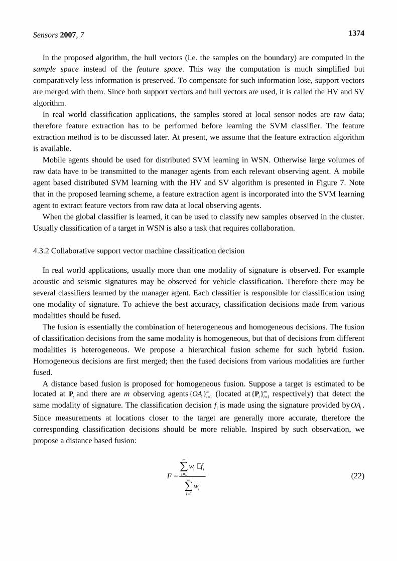
A distance based fusion is proposed for homogeneous fusion. Suppose a target is estimated to be located at sP and there are m observing agents 1{ } m

i iOA = (located at 1{ } mi i =P respectively) that detect the

same modality of signature. The classification decision if is made using the signature provided byiOA .

Since measurements at locations closer to the target are generally more accurate, therefore the

corresponding classification decisions should be more reliable. Inspired by such observation, we

propose a distance based fusion:

1

1

m

i ii

m

ii

w fF

w

=

=

⋅=∑

∑ (22)

Sensors 2007, 7

1375

1i

s i

w =−p p

(23)

Here iw is the weight for decisionif , and F is the homogeneously fused decision.

Now that homogeneous fusion has been finished, heterogeneous fusion can be embarked. Generally

heterogeneous fusion depends on a priori knowledge of the confidence associated with different

modalities. From experience, it is known that different modalities of signatures produce different

classification accuracy. A straightforward fusion scheme is placing more confidence on the modalities

producing better accuracy. This is achieved by setting larger weights just as the approaches for

homogeneous fusion. Suppose there are k modalities whose homogeneously fused decisions are ( )1rF r k≤ ≤ respectively. Assume classification accuracy concerning each modality rM is known a

priori and denoted byrA . Under such assumption, heterogeneous fusion is achieved by

1

1

k

r rr

k

rr

A FF

A

=

=

⋅=∑

∑ (24)

A final remark on heterogeneous fusion is that classification accuracyrA may be obtained by testing

the corresponding SVM classifier with known samples (i.e. whose labels are known a priori).

In the above discussions, it is supposed that the feature extraction method is available. In the

following section, it will be shown how the features are extracted from raw data.

4.3.3 Feature extraction with wavelet packet

Feature extraction is problem specific varying from application to application. That is why it is

supposed to be available in the preceding discussion. In this paper, we focus on extracting features

from acoustic and seismic signatures.

To extract their features, the characteristics of acoustic and seismic signals have to be investigated

first. A real world seismic signature is presented in Figure 8. Obviously the signature shown are

noticeably noised and non-stationary. The transient characteristics of the observed signature make

classical spectral methods like Fourier transformation unsuitable for efficient analysis. In [25], it is

proposed to use wavelet packet decomposition (WPD) for feature extraction. WPD provides detailed

information of a transient signature in both time and frequency domain by decomposing it into several

successive sub-band signals. An energy based WPD feature extraction method is proposed in this paper

following the same WPD principle in [24]. It is briefly summarized as follows.

Sensors 2007, 7

1376

Figure 8. Seismic signal observed by a seismic sensor in a real world WSN deployment.

First the signature is decomposed by WPD using the wavelet packet db4 at level 3. This results in 8

consecutive sub-band signals, denoted by3 ( ), ( 1,2,...8)iS t i = respectively. Then energy iE of 3 ( )iS t is

calculated by 2

3 ( )i iE S t dt= ∫ . Finally the feature vector is constructed by combining energy of these

sub-bands as 1 2 8' [ , , ... , ]F E E E= . Practically 'F is usually normalized to '/ max( ')F F F= . The

decomposed sub-band signals of the signature in Figure 8 are shown in Figure 9. In the figure, 1S is the

sub-band signal of the lowest frequency and 8S is the highest. Energy distribution among these

frequency bands varies with the type of the target that generates the seismic vibration; therefore feature

vectors composed of the sub-band energy can represent the characteristics of the target.

In the formulation of agent collaborative localization and classification algorithms, some approaches

and methods are intuitively proposed (not theoretically established). Real world target localization and

classification experiments are required to evaluate their validity.

Figure 9. Wavelet packet decomposition of the seismic signal shown in Figure 8.

Sensors 2007, 7

1377

5. Experiments

5.1. Experimental setup

In this section the proposed agent collaborative algorithms are evaluated in a real world WSN

deployment for vehicle localization and classification. The experiments are carried out on a schoolyard.

Big toy tanks and jeeps are used to simulate real vehicles. The WSN comprises 8 MICAz motes from

MICAz mote developer’s kit (a commercial product of Crossbow Inc.) [26]. The MICAz is a 2.4GHz,

IEEE 802.15.4 compliant module used for enabling low-power, wireless sensor networks. The mote

offers sensor boards that can measure signatures such as acoustic, acceleration and so forth [26]. In the

experiments, acoustic signatures are measured by the acoustic sensors provided by the MICAz sensor

board. However the mote is not equipped with sensors for seismic signatures; therefore seismic sensors

are artificially connected to the mote through its sensor board interface. Moreover the MICAz motes

are programmed to sample at the frequency of 1.024 kHz to accommodate acoustic and seismic

signatures of high frequency.

In the experiment, the 8 MICAz motes are randomly deployed on the schoolyard as illustrated in

Figure 10. As shown in the figure, the 8 motes denoted by s1, s2 through s8 are deployed within an

area approximately in the size of26 36m m× . Their corresponding x and y coordinates in the Cartesian

coordinate system are marked in the parentheses. The star in the figure denotes an imaginary target.

Following the proposed heterogeneous agent architecture, s1 through s7 are configured to be

observing agents and s8 is programmed to take the role of a manager agent. Meanwhile s8 is connected

to a laptop, which therefore also serves as the interface agent. In this configuration, the system can be

viewed as a miniature implementation of the proposed heterogeneous agent architecture, though only 8

sensor nodes are available.

A final remark on the deployment is that s8 will not participate in measurements of any kind. It is

solely responsible for coordination of the observing agents and dispatch of mobile agents.

Figure 10. Deployment of MICAz motes on the schoolyard for vehicle localization and classification.

Sensors 2007, 7

1378

5.2. Agent collaborative vehicle localization experiments

In the localization experiment, the vehicle is a toy tank emitting loud sound. It is kept stationary

during the localization. Nevertheless it must be clarified that the proposed method is equally applicable

to localization of moving vehicles. In one experiment, the vehicle is deployed at a position whose

Cartesian coordinates are (-4, 3). This is exactly where the target is in Figure 10. The acoustic

signatures measured by microphone sensors at s1, s2 and s3 (shown as examples) are shown in Figure

11. The signatures have all been processed to eliminate the influence of sensor gain discrepancy.

Following the proposed localization algorithms, s1, s2, s3 and s5 (reporting the highest average

energy) are selected to collaborate. The average energy and the positions of these observing agents are

used to determine the objective function (20). The steepest descent search is carried out by the manager

agent s8. The search result is reported in Figure 12. In the search, the termination condition is set to be

0.005, while the maximum search step is assigned to be 100. Numerical calculation shows no

relaxation of termination condition is needed. The search starts from the position of s1 which reports

the highest average energy. It takes only 10 steps to converge to the estimated location (-4.89, 2.52).

The estimate is 1.05m away from the true position. The distance between s1 and the target is 10.97m,

therefore the relative localization error is no more than1.05/10.97 100%=9.57 %× . This result proves the

proposed agent collaborative algorithm can efficiently perform vehicle localization in WSN.

As pointed out in the formulation of the agent collaborative algorithm, the selection of agents

involved in the objective function (20) is actually by intuition. To compare with the intuitive approach

an experiment using the 4 agents giving the lowest average energy is conducted. The result is shown in

Figure 13. As shown in the figure, s4, s5, s6 and s7 (reporting the lowest average energy) are chosen

for collaboration and the search is started from s5 (reporting the highest average energy among the 4

agents). It takes 11 steps to converge to the estimated location (-3.07, 1.91) which is 1.43m away from

the actual position. Again no relaxation of termination condition is deed.

Note that the proposed algorithm needs 10 steps and the estimated position is 1.05m from the true

location. By comparison, localization using the 4 agents with the highest average energy requires less

search steps and provides better localization accuracy. Therefore the proposed search method is time

efficient and accurate. Further evaluation of the proposed search method (i.e. searching with the agents

reporting highest average energy) is carried out by localizing vehicles randomly positioned within the

sensor field as shown in Figure 14.

As shown in Figure 14, 9 locations (denoted by T1 through T9, and marked by stars) are randomly

chosen. Their corresponding estimated locations are denoted by E1 through E9 respectively (marked by

diamonds). It shows that the algorithm can accurately localize vehicles at randomly selected position.

Note that some of the localization results (like E1, E3, E6 and E8) are more accurate than others. This

is due to differences in the relative positions between deployed sensor nodes and the vehicles.

The efficiency and accuracy of the proposed agent collaborative localization algorithm has been

validated by these experiments. Its good localization accuracy also benefits the agent collaborative

classification because the proposed homogeneous classification decision fusion is based upon the

estimated position of the target.

Sensors 2007, 7

1379

Figure 11. Acoustic signatures measured by microphones at s1, s2 and s3.

Figure 12. Vehicle localization by collaboration between s1, s2, s3 and s5.

Figure 13. Vehicle localization by collaboration between s4, s5, s6 and s7.

Sensors 2007, 7

1380

Figure 14. Agent collaborative localization of randomly positioned vehicles in the sensor field.

5.3. Agent collaborative vehicle classification experiments

The vehicle classification experiments are performed using the same deployment in Figure 10. The

vehicles to be classified are either toy tanks or jeeps. To achieve better classification accuracy, both

acoustic and seismic signatures are observed by MICAz motes. In our implementation, s1, s3, and s5

are programmed to measure acoustic signatures, while s2, s4 and s6 are configured to measure seismic

signals. Once again s8 serves as the manager agent and interface agent. Note that s7 is not used. Such

choice is to maintain the equilibrium between agents measuring acoustic signatures and the ones

measuring seismic signatures.

Learning samples are prepared in a supervised approach. Different vehicles are placed at various

positions. The seismic and acoustic signals are accordingly measured and stored by corresponding

observing agents. Meanwhile an operator determines the vehicle type and instructs the manager agent

to send vehicle type information to the observing agents. This ensures the locally gathered samples are

correctly labeled. All sampling lasts for 2 seconds. Recall that the sampling frequency is 1.024 kHz;

therefore each sample contains 2048 sample points.

When samples are prepared, the proposed distributed SVM learning can be started. Mobile agents

are sent from the manager agent s8 to observing agents s1 through s6 to extract features, learn local

SVM classifiers and compute hull vectors. Radial basis function (RBF) is used as the kernel for SVM

learning.

Typical acoustic features of toy tanks and jeeps are demonstrated in Figure 15. In the figure, Sn

denotes the nth component of the feature vector and normalized energy is expressed in logarithm

coordinate. Evidently the features make these two types of toy vehicles distinguishable, but such

features are more than enough to separate toy tanks from jeeps. For example, the first component s1 is

identical for both vehicles; therefore it contributes extremely little, if any at all, to the discrimination of

the vehicles. Following the same principle, components s4, s5 and s6 are negligible too, because these

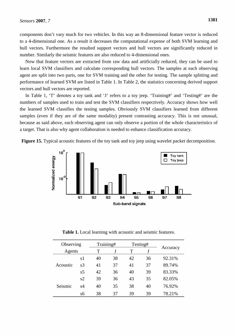
Sensors 2007, 7

1381

components don’t vary much for two vehicles. In this way an 8-dimensional feature vector is reduced

to a 4-dimensional one. As a result it decreases the computational expense of both SVM learning and

hull vectors. Furthermore the resulted support vectors and hull vectors are significantly reduced in

number. Similarly the seismic features are also reduced to 4-dimensional ones.

Now that feature vectors are extracted from raw data and artificially reduced, they can be used to

learn local SVM classifiers and calculate corresponding hull vectors. The samples at each observing

agent are split into two parts, one for SVM training and the other for testing. The sample splitting and

performance of learned SVM are listed in Table 1. In Table 2, the statistics concerning derived support

vectors and hull vectors are reported.

In Table 1, ‘T’ denotes a toy tank and ‘J’ refers to a toy jeep. ‘Training#’ and ‘Testing#’ are the

numbers of samples used to train and test the SVM classifiers respectively. Accuracy shows how well

the learned SVM classifies the testing samples. Obviously SVM classifiers learned from different

samples (even if they are of the same modality) present contrasting accuracy. This is not unusual,

because as said above, each observing agent can only observe a portion of the whole characteristics of

a target. That is also why agent collaboration is needed to enhance classification accuracy.

Figure 15. Typical acoustic features of the toy tank and toy jeep using wavelet packet decomposition.

Table 1. Local learning with acoustic and seismic features.

Training# Testing# Observing

Agents T J T J Accuracy

s1 40 38 42 36 92.31%

s3 41 37 41 37 89.74% Acoustic

s5 42 36 40 39 83.33%

s2 39 36 43 35 82.05%

s4 40 35 38 40 76.92% Seismic

s6 38 37 39 39 78.21%

Sensors 2007, 7

1382

In table 2, ‘SV#’ denotes the number of support vectors (SV), ‘HV #’ means the number of hull

vectors (HV). ‘HSV #’ refers to the number of the vectors in the union of support vectors and hull

vectors. We are most interested in the difference between SV# and HSV#. Because SV# indirectly

represents the transmitted data volume for the SV only algorithm and HSV #corresponds to that of the

HV and SV algorithm. In all cases, HSV# is larger than SV#, which is expected by theoretical analysis.

Accordingly the HV and SV algorithm consumes more energy for communication between the

manager and observing agents. As noted before, hull vectors are incorporated to improve distributed

learning accuracy. Now let us turn to see its learning performance as shown in Table 3.

In the table, ‘Centralized’ refers to the traditional centralized learning algorithm that sends all

samples to a central point and learns the global SVM classifier accordingly. Evidently the centralized

algorithm performs the best for both modalities, because it has access to all available samples. The HV

and SV algorithm is almost as good as the centralized algorithm. In contrast, the SV only algorithm

performs much worse than the centralized. For acoustic features, it is nearly 7% worse than the

centralized. For seismic, it is almost 10% worse in performance.

Therefore as far as learning accuracy is concerned, the HV and SV algorithm proposed in this paper

is superior to the SV only algorithm. However just as shown in Table 2, the accuracy improvement is

at the cost of increase in communication load. Usually such tradeoff is desirable, because in

classification applications, accuracy is of the highest priority compared to other factors like energy

consumed by wireless communication.

Table 2. The numbers of support vectors, hull vectors and their unions.

SV# HV# HSV# Observing

Agents T J T J T J

s1 29 13 26 22 36 26

s3 35 9 30 26 38 26 Acoustic

s5 29 13 26 22 36 26

s2 17 17 28 19 32 25

s4 19 19 24 25 32 32 Seismic

s6 18 18 24 24 32 30

Table 3. Learning performance of different algorithms and modalities.

Learning Algorithm Training# Testing# SV# Accuracy

SV only 126 234 41 88.46%

HV and SV 188 234 35 93.59% Acoustic

Centralized 156 312 64 95.19%

SV only 108 234 108 74.79%

HV and SV 183 234 93 83.33% Seismic

Centralized 156 312 64 84.29%

Sensors 2007, 7

1383

Furthermore it should be noted that data transmission has been drastically decreased by mobile

agents. Feature extraction and the HV and SV algorithm both perform data compression. Take

transmission of raw data of s1 for example. All together, 624kByte raw data have to be transmitted

(note that, a double point takes 4 bytes; each raw sample is 2048*4 bytes; there are 40+38 samples all

together). However, for the HV and SV algorithm using mobile agents, only 0.248kByte data (volume

of the derived 4-dimensional hull vectors and support vectors) need to be transmitted. Even if dispatch

of mobile agents is taken into account, the data transmission is still much smaller than 624kBytes.

Now that global SVM classifiers have been learned at the manager agent using acoustic and seismic

features respectively, they can be used to classify unknown targets detected in the sensor field.

The classification of an unknown target is relatively easier than the learning of the classifier itself.

When a target is detected and located, the manager agent instructs the observing agents to measure

either acoustic or seismic signatures. Then mobile agents for feature extraction are sent to these

observing agents. The extracted features are sent back to the manager agent where homogeneous and

heterogeneous fusions are carried out to make the fused classification decision.

In the experiment, s1, s3 and s5 measure acoustic signature; s2, s4 and s6 observe seismic signatures.

A toy tank is place at position (-4,-5) whose estimated position is (-5.3, -4.3). The homogeneous and

heterogeneous fusion results are presented in Table 4 following the proposed fusion algorithms.

In the table, the weight for homogenous fusion is determined following (23) but normalized. The

modality weight for heterogeneous fusion is determined upon their classification performance. In this

experiment, as shown in Table 3, the classification accuracy is 93.59% (using the HV and SV

algorithm) for acoustic modality and 83.33% for seismic modality. Therefore the normalized modality

weight for acoustic classification is 93.59% / (93.59%+83.33%) =0.529. The seismic modality weight

is similarly calculated.

According to the decision rule, a positive decision means a toy tank while a negative one means a

toy jeep. For acoustic classification, s1 and s3 believe the target is a toy tank, but s5 reports it as a toy

jeep. Disputes arise and fusion needs to be made to form a more reliable decision. The situation is

similar for seismic classification. Homogeneous fusion results are further fused following (24) and the

final decision is 1.0638. It means the global fusion decision is a toy tank. Such decision is in

accordance with the truth, for it is known a priori that the target is a toy tank.

Table 4. Fusion results of agent collaborative classification decisions.

Homogeneous Fusion Modality

Modality

Weight Agent

Decision Weight Fusion

Hetero-

geneous

Decision

s1 1.6405 0.2459

s3 2.2360 0.5344 Acoustic 0.529

s5 -1.9544 0.2196

1.1692

s2 0.9673 0.4894

s4 1.8766 0.3373 Seismic 0.471

s6 -0.9279 0.1733

0.9455

1.0638

Sensors 2007, 7

1384

The fusion results in Table 4 show that local decision may be incorrect, but following the proposed

fusion algorithm a reliable global decision is obtained. Therefore the proposed method is efficient to

perform hierarchical fusion of both homogenous and heterogeneous decisions.

As corroborated by the experiment results, the proposed heterogeneous agent architecture

significantly facilitates designs of WSN and remarkably reduces in-network communication load. With

this architecture, the proposed localization and classification algorithms are easily implemented and

prove to be accurate and energy efficient.

6. Conclusions

This paper proposes to model WSN as a heterogeneous agent system. With this architecture, target

localization and classification tasks are implemented through agent collaboration. The developed agent

system is basically a 4 level hierarchical multi-agent system where mobile agents are employed when

necessary and beneficial. Both target localization and classification tasks in WSN essentially require

some kinds of collaboration. As shown in the paper, it is very convenient to achieve such collaboration

through the proposed agent architecture. Practically various forms of collaboration are possible.

Therefore much effort in the paper is devoted to develop the appropriate collaboration mechanisms.

These mechanisms should provide desirable accuracy and at the same adapt to WSN constraints like

limited power supply and bandwidth. Based upon this rationale, energy based acoustic localization by

multi-agent collaboration is proposed, because it requires less in-network communication. In the

proposed SVM classification method, hull vectors are used to guarantee good accuracy and meanwhile

keep communication load as low as possible. The integration of mobile agents drastically reduces data

exchange by transmitting codes instead of raw data. As confirmed by the experiment results, the

heterogeneous agent architecture remarkably simplifies application designs and collaborative algorithm

implementations. It is also proved that the proposed agent collaborative algorithms for localization and

classification are accurate and energy efficient.

Acknowledgements

This paper is supported by the National Grand Fundamental Research 973 Program of China under

Grant No.2006CB303000 and National Natural Science Foundation of China under Grant

No.60673176, No.60373014 and No.50175056.

References and Notes

1. Estrin, D.; Girod, L.; Pottie, G.; Srivastava, M. Instrumenting the world with wireless sensor

network. Proc. ICASSP’2001, 2001, 2675-2678.

2. Estrin, D.; Culler, D.; Pister, K.; Sukhatme, G. Connecting the physical world with pervasive

networks. IEEE Pervasive Computing, 2002, 1(1), 59-69.

3. Li, D.; Wong, K.D.; Hu, Y.H.; Sayeed, A.M. Detection, classification and tracking of targets.

IEEE Signal Processing Magazine, 2002, 19, 17–29.

Sensors 2007, 7

1385

4. Li, D.; Hu, Y.H. Energy based collaborative source localization using acoustic micro-sensor array.

EURASIP Journal on Applied Signal Processing, 2003, 4, 321-337.

5. Huang, Y.; Benesty, J.; Elko, G.W.; Mersereau, R.M. Real-time passive source localization: A

practical linear-correction least-squares approach. IEEE Trans. Speech Audio Processing, 2001, 9(8), 943-956.

6. Lehmann, E.A.; Ward, D.B.; Williamson, R.C. Experimental comparison of particle filtering

algorithms for acoustic source localization in a reverberant room. Proc. 2003 IEEE International

Conference on Acoustics, Speech, and Signal Processing, 2003, 5, 375-380.

7. Marco, F.D.; Yu, H.H. Vehicle classification in distributed sensor networks. Journal of Parallel

and Distributed Computing, 2004, 64, 826–838.

8. Wang,X.; Wang, S. Collaborative signal processing for target tracking in distributed wireless

sensor networks. Journal of Parallel and Distributed Computing, 2007, 67(5), 501-515.

9. Liu,J.; Reich, J.; Zhao, F. Collaborative in-network processing for target tracking. EURASIP

Journal on Applied Signal Processing, 2003, 4, 378-391.

10. Xu, Y. Distributed computing paradigms for collaborative signal and information processing in

sensor networks. Journal of Parallel and Distributed Computing, 2004, 64(8), 945–959.

11. Qi, H.; Wang, X.; Iyengar, S.S.; Chakrabarty, K. Multisensor data fusion in distributed sensor

networks using mobile agents. Proceedings of International Conference on Information Fusion,

2001, 11-16.

12. Panait, L.; Luke, S. Cooperative multi-agent learning: the state of the art. Autonomous Agents and

Multi-Agent Systems, 2005, 11(3), 387–434.

13. Shakshuki, E.; Ghenniwa, H.; Kamel, M. Agent-based system architecture for dynamic and open

environments. Journal of Information Technology and Decision Making, 2003, 2(1), 105-133.

14. Hussain, S.; Shakshuki, E.; Matin, A.W. Agent-based system architecture for wireless sensor

networks. 2006 Proc. 20th International Conference on Advanced Information Networking and

Applications, 2006, 2, 18-20.

15. Wang, X.; Wang, S. An improved particle filter for target tracking in sensor system. Sensors, 2007, 7(1), 144 -156.

16. Knapp, C.H.; and Carter, G.C. The generalized correlation method of estimation of time delay.

IEEE Trans. on Acoustics, Speech, and Signal Processing, 1976, 24(4), 320-327.

17. V. Vapnik, the Nature of Statistical Learning Theory, New York: Springer, 1998. 18. Burges, C.J.C. A tutorial on support vector machines for pattern recognition. Data Mining and

Knowledge Discovery, 1998, 2, 21-167.

19. Caragea, C.; Caragea, D.; Honavar, V. Learning support vector machine classifiers from

distributed data sources. Proc. of the Twentieth National Conference on Artificial Intelligence,

2005, 1602-1603.

20. Syed, N.; Liu, H.; and Sung, K. Incremental learning with support vector machines. Proc. of

Workshop on Support Vector Machines at the International Joint Conference on Artificial

Intelligence, 1999，272-276.

21. Osuna, E; Castro, O.D. Convex hull in feature space for support vector machines. Lecture Notes in

Computer Science, 2002, 2527/2002, 411-419.

Sensors 2007, 7

1386

22. Rawlins, G.J.E.; Wood, D.: Ortho-convexity and its generalizations. Computational Morphology,

1988, 137-152.

23. Moses, R.L.; Krishnamurthy, D.; Patterson, R. A self-localization method for wireless sensor

networks. EURASIP Journal on Applied Signal Processing, 2003, 4, 348-358.

24. Polak, E.: Optimization: Algorithms and Consistent Approximations. Springer-Verlag, 1997. 25. Averbuch, A.; Hulata, E.; Zheludev, V. Wavelet packet algorithm for classification and detection

of moving vehicles. Multidimensional Systems and Signal Processing, 2001, 12(1), 9-31.

26. MICAz Datasheet, Crossbow Technology Inc., San Jose, California, 2006.

© 2007 by MDPI (http://www.mdpi.org). Reproduction is permitted for noncommercial purposes.