agglomeration and demographic change - etsg · agglomeration and demographic change theresa...
TRANSCRIPT

Agglomeration and demographic change
Theresa Grafeneder-Weissteiner∗, Klaus Prettner†
Preliminary version
July 15, 2009
Abstract
This article investigates common consequences of population agingand economic integration for agglomeration. We introduce demogra-phy into the New Economic Geography by generalizing the constructedcapital approach to account for finite planning horizons. Interestingly,the level of trade costs triggering agglomeration is rather sensitive tochanges in mortality. In particular, we find that a positive mortalityrate counteracts concentration of industrial activity. In sharp contrastto other New Economic Geography approaches, agglomeration pro-cesses may thus not set in even if economic integration is promoted upto a high degree.
JEL classification: F12; F15; C61Keywords: Agglomeration; Constructed Capital Model; PopulationAging
∗Vienna University of Economics and Business Administration, Department of Eco-nomics, Augasse 2-6, A-1090 Vienna, Austria; email: [email protected]; tel: +43 131336 4088; fax: +43 1 31336 9209†Vienna Institute of Demography, Austrian Academy of Sciences, Wohllebengasse 12-
14, A-1040, Vienna, Austria and Institute of Mathematical Methods in Economics, ViennaUniversity of Technology, Argentinierstrasse 8/4/105-3, A-1040 Vienna, Austria; email:[email protected]; tel: +43 1 51581 7729; fax: +43 1 51581 7730
1
1 Introduction
Over the last decades, most economies have been confronted with tremen-dous structural changes arising from globalization and demographic devel-opments. Freer trade (see Sachs and Warner (1995)) has led to higher inter-national integration meaning that goods produced in a certain region cannowadays be sold all over the world at a more competitive price. As a re-sult, global competition for productive factors has emerged. In particular,firms have started to invest in regions where productive factors are rela-tively cheap and ship their goods to regions populated by consumers withhigh purchasing power. This emphasizes the linkage between relocation ofmanufacturing to areas with high rates of return on capital on the one handand deeper economic integration on the other hand.
At the same time, fertility rates have decreased in nearly all countries(see Eurostat (2004)) resulting in lower population growth rates and agingsocieties (see United Nations (2007)). These demographic developments donot only change the productivity of labor but also have crucial impacts onthe demand and saving patterns in the economy which in turn affect thereturns of productive factors. As a consequence, economic integration anddemographic change are inseparably linked with each other. Despite thisfact, their common economic consequences have barely been analyzed inone single framework up to now. Our paper closes the gap by introducingdemography into the New Economic Geography. We are thus able to de-scribe the effects of declining transport costs on the location of productivefactors in a setting with aging populations. In particular, our model revealswhether concentration of economic activity as emphasized by the New Eco-nomic Geography literature still takes place when allowing for finite planninghorizons.
The New Economic Geography literature pioneered by Krugman (1991),Venables (1996) and Krugman and Venables (1995) provided new insightsinto how transport costs can determine the spatial distribution of economicactivity. These models are characterized by catastrophic agglomerationmeaning that for certain threshold levels of economic integration, indus-trial activity completely concentrates in one region. In particular, circularcausality effects between factor rewards and demands for monopolisticallycompetitive goods encourage agglomeration processes. They destabilize the
2
symmetric equilibrium with an equal division of productive factors and turnthe core-periphery outcome with all industrial activity taking place in oneregion into a stable equilibrium. Reciprocal liberalization between initiallysymmetric regions that strengthens such circular causality effects thus leadsto complete deindustrialization of one region.
Puga (1999) set up a model that nested as special cases both the Krug-man (1991) framework with labor mobility between regions as well as thevertically linked-industries model of Venables (1996) and Krugman and Ven-ables (1995) without interregional labor mobility. However, the richness ofagglomeration features in these models reduced their analytical tractabil-ity. Therefore Baldwin (1999) introduced the constructed capital frameworkwith interregional labor and capital immobility but forward-looking agents.His model features catastrophic agglomeration of capital stocks explainedby the difference in the capital rental rates of two regions. A higher rentalrate in the home region causes home capital accumulation, whereas capitalis decumulated in the foreign region. The only force fostering this agglom-eration process is a demand-linked circular causality effect setting in as ahigher capital stock raises capital income and thus expenditures which leadsto a further increase in home rental rates. Since neoclassical growth modelsin the spirit of Ramsey (1928) and Solow (1956) associate capital accu-mulation with medium-run growth, Baldwin (1999) describes the economyaccumulating capital as a growth pole, whereas the other region appears as agrowth sink. His agglomeration induced growth story therefore nicely illus-trates how economic integration strengthening the demand-linked circularcausality could lead to the development of “rust” and “boom belts”.
In contrast to the Ramsey (1928) framework of one single, infinitelylived, representative agent, on which the constructed capital model’s savingfeatures heavily rely, agents do not live forever in reality. We therefore gen-eralize Baldwin (1999)’s approach by introducing the possibility of deathand thus accounting for finite planning horizons. In doing so, we adoptBlanchard (1985)’s structure of overlapping generations, where heterogene-ity among individuals is due to their date of birth. While still following thelines of intertemporally optimizing agents, this results in a more compre-hensive model incorporating life-cycle decisions and nesting the constructedcapital set-up as a special case. Since demographic structures influence thesaving patterns in the economy, the introduction of mortality affects the
3

capital rental rate and plays a crucial role for agglomeration processes. Themodel presented in this paper therefore reveals in detail the linkages betweenpopulation aging, economic integration and agglomeration.
Our results show that the introduction of finite planning horizons weak-ens agglomeration tendencies between two regions. The possibility of deathacts as an additional dispersion force against the concentration of indus-trial activity by lowering the positive effect of an increased capital stock onthe capital rental rate. In particular, we find that a higher mortality rateconsiderably reduces the possibility of the symmetric equilibrium to be un-stable. This implies that Baldwin (1999)’s agglomeration induced growthfinding primarily applies in the very special case of infinitely lived individu-als and that agglomeration processes in aging societies may not set in evenif economic integration is promoted up to a high degree.
The paper proceeds as follows. Section 2 presents the structure of themodel and derives optimal saving behavior and the equilibrium capital rentalrate of the economy. Section 3 verifies the existence of a symmetric long-runequilibrium and characterizes its properties with respect to the mortalityrate. Section 4 establishes the link between agglomeration and demographicchange. To complement our analytical findings by numerical illustrations wealso calibrate the model for reasonable parameter values. Finally, section 5summarizes and draws conclusions for economic policy.
2 The model
This section describes how we integrate Blanchard (1985)’s notion of finiteplanning horizons into the constructed capital framework of Baldwin (1999).Consumption and savings behavior as well as production technologies areintroduced and various intermediate findings resulting from profit maximiza-tion are presented. In order to be able to analyze the long-run equilibrium,we also derive aggregate laws of motion for capital and expenditures.
2.1 Basic structure and underlying assumptions
The model consists of two symmetric regions or countries, referred to as Hfor home and F for foreign1, with identical production technologies, prefer-
1If further distinction is needed, foreign variables are moreover indicated by an asterisk.In particular, the superscript F denotes that a good was produced in the foreign region,
4

ences of individuals, labor endowments and demographic structures. Eachregion has three economic sectors (agriculture, manufacturing and invest-ment) with two immobile factors (labor L and capital K) at their disposal.The homogeneous agricultural good, n, is produced in a perfectly competi-tive market with labor as the only input and can be traded between the tworegions without any cost. Manufacturing firms are modeled as in the mo-nopolistic competition framework of Dixit and Stiglitz (1977) and thereforeproduce varieties, m, with one unit of capital as fixed input and labor as thevariable production factor. A continuum of varieties i ∈ (0, VH ] is producedat home, whereas a continuum of varieties j ∈ (0, VF ] is manufactured in theforeign region. In contrast to the agricultural good, trade of manufacturesinvolves iceberg transport costs such that ϕ ≥ 1 units of the differentiatedgood have to be shipped in order to sell one unit abroad (see e.g. Baldwinet al. (2003)). In the Walrasian investment sector, capital, i.e. machines,are produced using labor as the only input where wages are paid out of theindividuals’ savings. The failure rate of a machine is assumed to be inde-pendent of the machine’s age. Denoting this failure rate as 0 < δ ≤ 1, andusing the law of large numbers, implies that the overall depreciation rate ofcapital is given by δ as well.
As far as the demographic structure of our model economy is concerned,we closely follow Blanchard (1985)’s simplified setting. We assume that ateach point in time, τ ∈ [0,∞), a large cohort consisting of new individuals isborn. These newborns receive no bequests and thus start their lives withoutany wealth. The size of this cohort is N(τ, τ) = µN(τ), where 0 < µ ≤ 1 isthe constant birth rate and N(τ) ≡
∫ τ−∞N(t0, τ)dt0 is total population at
time τ with N(t0, τ) denoting the size of the cohort born at t0 for any givenpoint in time τ .2 Consequently, cohorts can be distinguished by the birthdate t0 of their members. Since there is no heterogeneity between membersof the same cohort, each cohort can be described by one representativeindividual, who inelastically supplies his efficiency units of labor at the labormarket with perfect mobility across sectors but immobility between regions.The age of the individual is given by a = τ − t0 and his time of death isstochastic with an exponential probability density function. In particular,
whereas the asterisk indicates that it is consumed in the foreign region.2In what follows the first time index of a variable will refer to the birth date, whereas
the second will indicate a certain point in time.
5

the probability of death is also given by the age independent parameter µresulting in a surviving probability to age τ − t0 of e−µ(τ−t0). Since thepopulation size is large, the frequency of dying is equal to the instantaneousmortality rate. Therefore the number of deaths at each point in time isµN(τ). As this equals, by assumption, the number of births, populationsize is constant and can be normalized to one. Finally, as in Yaari (1965), aperfect life-insurance company offers actuarial notes, which can be boughtor sold by each individual and are canceled upon the individual’s death.
2.2 Individual utility optimization
Preferences over the agricultural good and a CES composite of the man-ufacturing varieties are Cobb-Douglas.3 The representative individual ofcohort t0 chooses at each instant τ > t0 consumption of the agriculturalgood, cn(t0, τ), consumption of varieties produced at home, cHm(i, t0, τ), andconsumption of varieties produced abroad, cFm(j, t0, τ), to maximize his ex-pected lifetime utility at time t04
U(t0, t0) =∫ ∞t0
e−(ρ+µ)(τ−t0) ln[(cn(t0, τ))1−ξ(caggm (t0, τ))ξ
]dτ, (1)
where ρ > 0 is the pure rate of time preference, 0 < ξ < 1 is the manufac-turing share of consumption and
caggm (t0, τ) ≡
[∫ VH(τ)
0
(cHm(i, t0, τ)
)σ−1σ di+
∫ VF (τ)
0
(cFm(j, t0, τ)
)σ−1σ dj
] σσ−1
represents consumption of the CES composite with σ > 1 denoting theelasticity of substitution between varieties.
Individual savings, defined as income minus consumption expenditures,are converted into capital in the investment sector with a time indepen-dent, exogenous labor input coefficient of F . The wealth constraint of a
3The following discussion refers to the home region but due to symmetry, equivalentequations also hold in the foreign region.
4Equation (1) can be easily derived by calculating expected lifetime utility where thedate of death is a random variable with an exponential probability density function pa-rameterized by a constant instantaneous mortality rate µ.
6

representative individual can be thus written as
k(t0, τ) =w(τ)l(τ) + π(τ)k(t0, τ)− e(t0, τ)
w(τ)F+ µk(t0, τ)− δk(t0, τ), (2)
where w(τ) denotes the wage per efficiency unit of labor, l(τ) refers to theage independent efficiency units of labor an individual supplies, π(τ) is thecapital rental rate, k(t0, τ) the individual capital stock of an individual ande(t0, τ) are individual total expenditures for consumption defined as
e(t0, τ) ≡ pn(τ)cn(t0, τ) +∫ VH(τ)
0pHm(i, τ)cHm(i, t0, τ)di+∫ VF (τ)
0pFm,ϕ(j, τ)cFm(j, t0, τ)dj.
Here pn(τ) is the price of the agricultural good, pHm(i, τ) the price of a manu-factured variety produced at home and pFm,ϕ(j, τ) the price of a manufacturedvariety produced abroad with the subscript ϕ indicating the dependence ontransport costs.
The particular law of motion for capital given in equation (2) is based onYaari (1965)’s full insurance result implying that all individuals only holdtheir wealth in the form of actuarial notes.5 Therefore the market rate ofreturn on capital, π(τ)
w(τ)F − δ, has to be augmented by µ to obtain the fairrate on actuarial notes (see Yaari (1965)).
In appendix A we solve the individual’s utility optimization problem byapplying a three stage procedure. In the first stage the dynamic savings-expenditure decision is analyzed. Stage two deals with the static optimalconsumption allocation between the CES composite and the agriculturalgood and in stage three individuals decide upon the amount of consumptionthey allocate to each of the manufactured varieties. Altogether this leads tothe following demand functions for the agricultural good and for each of the
5Two interpretations of the capital accumulation process are therefore possible. Eithereach individual itself converts its savings into capital and then leaves it to the insurancecompany or savings are immediately transferred to the insurance company which convertsthem into machines by employing workers.
7

manufactured varieties
cn(t0, τ) =(1− ξ)e(t0, τ)
pn(τ), (3)
cHm(i, t0, τ) =ξe(t0, τ)(pHm(i, τ))−σ[∫ VH(τ)
0 (pHm(i, τ))1−σdi+∫ VF (τ)
0 (pFm,ϕ(j, τ))1−σdj] , (4)
cFm(j, t0, τ) =ξe(t0, τ)(pFm,ϕ(j, τ))−σ[∫ VH(τ)
0 (pHm(i, τ))1−σdi+∫ VF (τ)
0 (pFm,ϕ(j, τ))1−σdj] (5)
as well as to the consumption Euler equation for the representative individ-ual of cohort t0
e(t0, τ)e(t0, τ)
=π(τ)Fw(τ)
− δ − ρ. (6)
As first shown by Yaari (1965) the representative individual’s Euler equa-tion with fully insured lifetime uncertainty is identical to the Euler equationwhen no lifetime uncertainty exists, i.e. individual saving behavior is notinfluenced by the mortality rate and moreover does not differ across gener-ations.
2.3 Aggregate expenditures and capital
Due to the overlapping generations structure resulting from the introduc-tion of mortality into the constructed capital framework, our model setupdoes not feature one single representative individual. In order to be ableto analyze the long-run equilibrium of the economy as well as its stabilityproperties it is therefore necessary to derive the aggregate law of motions ofcapital and consumption expenditures. The capital stock of the economy ata certain point in time t can be obtained by aggregating up the capital stocksof all cohorts. An analogous definition applies to consumption expenditures.These aggregation rules are formally given by
K(t) ≡∫ t
−∞k(t0, t)N(t0, t)dt0, (7)
E(t) ≡∫ t
−∞e(t0, t)N(t0, t)dt0, (8)
8

where K(t) is the aggregate capital stock and E(t) denotes aggregate con-sumption expenditures6. Equivalent equations hold for the foreign region.
Using the demographic assumptions described in section 2.1 we can ex-actly trace the size N(t0, t) of any particular cohort over time. A cohortborn at time t0 is of size µe−µ(t−t0) at time t ≥ t0 as the probability ofsurviving to time t equals e−µ(t−t0) and the initial size of the cohort is µ.Substituting for N(t0, t) in equation (8) therefore yields
E(t) ≡ µ∫ t
−∞e(t0, t)e−µ(t−t0)dt0. (9)
The “aggregate Euler equation”, modified for the existence of overlappinggenerations of finitely lived agents, directly follows from equation (9) bydifferentiating it with respect to t and then substituting for e(t0, t) from theindividual Euler equation (6) and for e(t, t) and E(t) from the correspondingexpressions derived in appendix B where we describe the various aggregationsteps in detail.7 It is given by
E(t)E(t)
= −µ(ρ+ µ)Fw(t)K(t)E(t)
+π(t)w(t)F
− ρ− δ (10)
= −µE(t)− e(t, t)E(t)
+e(t0, t)e(t0, t)
. (11)
In sharp contrast to the individual Euler equation, the mortality rate playsa prominent role in the aggregate Euler equation. From equation (11) itfollows that the difference between individual and aggregate savings behav-ior is captured by a correction term representing the distributional effectsdue to the turnover of generations (see Heijdra and van der Ploeg (2002),chapter 16). Optimal consumption expenditure growth is the same for allgenerations (see equation (6)) but optimal expenditure levels differ. In par-ticular, allowing for finite planning horizons introduces heterogeneity amongindividuals with respect to their birth dates and, since wealth and consump-tion levels are age dependent, also with respect to their expenditures. Asshown in appendix B, optimal consumption expenditures e(t0, t) are propor-
6The aggregate efficiency units of labor L(t) are equal to the individual supply ofefficiency units of labor l(t) due to age independency and the normalization of populationsize to one.
7Those aggregation steps closely follow the ones described by Heijdra and van der Ploeg(2002) in chapter 16.
9

tional to total wealth with the marginal propensity to consume out of totalwealth being equal to the “effective” rate of time preference ρ+µ. Olderindividuals are wealthier due to their accumulated capital holdings andtherefore have higher consumption expenditure levels than their youngercounterparts. Since dying old generations are replaced by newborns with nocapital holdings at each point in time, aggregate consumption expendituregrowth is smaller than individual consumption expenditure growth. Thecorrection term on the right hand side of equation (10) therefore describesthe difference between average consumption expenditures8 and consumptionexpenditures by newborns as shown in equation (11). Since E(t) − e(t, t)is unambiguously positive (see appendix B), a higher mortality rate de-creases aggregate consumption expenditure growth. This is intuitively clearas a higher µ implies a higher generational turnover and therefore a morepronounced (negative) distributional impact. In the case of infinitely livedindividuals, i.e. µ = 0, the turnover effect completely disappears. Since themortality rate only enters the aggregate Euler equation via this turnovercorrection term, we can conclude that the introduction of finite planninghorizons influences aggregate saving patterns in the economy only by thedistributional effects resulting from the death. It is thus not surprising thatthis turnover channel will play a crucial role when it comes to investigatingthe linkage between the mortality rate and the forces fostering or weakeningagglomeration in our model.
Similarly, the aggregate law of motion for the capital stock can be ob-tained. Rewriting equation (7) in analogy to equation (9) and then differ-entiating it with respect to t yields
K(t) =[π(t)w(t)F
− δ]K(t) +
w(t)L(t)w(t)F
− E(t)w(t)F
, (12)
where we applied the same steps as in the derivation for the aggregate Eulerequation shown in appendix B.9 Compared to the law of motion for indi-vidual capital, there appears no term featuring the mortality rate µ. Thiscaptures the fact that µK(t) does not represent aggregate capital accumu-lation but is a transfer - via the life insurance company - from individuals
8Since we normalized total population size to 1, total consumption expenditures E(t)are equal to average consumption expenditures.
9In particular, we substituted for k(t0, t) from equation (2).
10

who died to those who survived within a given cohort. As a consequence,aggregate capital accumulates at a rate π(t)
w(t)F −δ, whereas individual capital
attracts the actuarial interest rate π(t)w(t)F + µ − δ for surviving individuals
(see Heijdra and van der Ploeg (2002), chapter 16).Summarizing, the mortality rate µ enters the law of motion for the in-
dividual capital stock but disappears in the corresponding aggregate law ofmotion. This is in sharp contrast to the Euler equation, where µ does notshow up at the individual level but is part of the aggregate consumptionexpenditure growth rate.
2.4 Production technology and profit maximization
Profit maximization in the manufacturing and agricultural sector closelyfollows Baldwin (1999) and yields various intermediate results that simplifythe subsequent analysis of the long-run equilibrium. In particular, the waythe manufacturing sector is modeled allows us to derive the rental rate ofcapital as a function of home and foreign capital stocks and expenditures.
2.4.1 Agricultural sector
The homogeneous agricultural good, which can be interpreted as food, isproduced according to the following constant returns to scale productionfunction
Yn(t) =1αLn(t), (13)
where Yn(t) denotes output of the agricultural sector, Ln(t) represents ag-gregate labor devoted to agricultural production, and α is the unit input co-efficient in the production of agricultural goods. Profit maximization underperfect competition implies that the price equals marginal costs. Moreover,by choice of units for agricultural output, α can be set to one implying thatthe wage rate equals the price of the agricultural good
pn(t) = wn(t). (14)
Since labor is perfectly mobile across sectors the wage rate in the economyw(t) satisfies
wn(t) = wm(t) = winv(t) = w(t), (15)
11

where wn(t), wm(t) and winv(t) denote wages in the agricultural, manu-facturing and investment sector. Therefore equation (14) pins down theequilibrium wage in the economy. As free trade of the agricultural good be-tween home and foreign equalizes its price, wages are also equalized betweenthe two regions as long as each of them produces some Yn(t). This can beshown to hold if ξ, the manufacturing share of consumption, is not too large(see Baldwin (1999)) which will be assumed from now on. Finally, choosingthe agricultural good as numeraire leads to
w(t) = w∗(t) = 1. (16)
2.4.2 Manufacturing sector
Each firm in the Dixit and Stiglitz (1977) monopolistically competitive man-ufacturing sector produces a different output variety using labor as variableand one variety-specific machine as fixed input. This machine originatesfrom the investment sector and is equivalent to one unit of capital. Due tothe fixed costs, firms face an increasing returns to scale production technol-ogy with an associated cost function
π(t) + w(t)βYm(i, t), (17)
where β is the unit input coefficient for efficiency units of labor, Ym(i, t) istotal output of one manufacturing good producer and the capital rental rateπ(t) represents the fixed cost.
Defining10 Pm(t) ≡∫ VH(t)
0 (pHm(i, t))1−σdi +∫ VF (t)
0 (pFm,ϕ(j, t))1−σdj andP ∗m(t) ≡
∫ VF (t)0 (pHm(j, t))1−σdj+
∫ VH(t)0 (pFm,ϕ(i, t))1−σdi and recognizing that
each individual firm has mass zero and hence does not influence the priceindexes Pm and P ∗m, leads to the following maximization problem for each
10Note that pHm(j, t) = p∗Fm (j, t) and pFm,ϕ(i, t) = p∗Hm,ϕ(i, t) due to symmetry betweenthe two regions, where p∗Hm,ϕ(i, t) is the price of a good produced in the home economy butconsumed in the foreign region.
12

firm at time t11
maxpHm,p
Fm,ϕ
(pHm(i, t)− w(t)β)(∫ t
−∞cHm(i, t0, t)N(t0, t)dt0
)+(pFm,ϕ(i, t)− w(t)ϕβ)
(∫ t
−∞cH∗m (i, t0, t)N∗(t0, t)dt0
)s.t. cHm(i, t0, t) =
ξe(t0, t)(pHm(i, t))−σ
Pm(t)
cH∗m (i, t0, t) =ξe∗(t0, t)(pFm,ϕ(i, t))−σ
P ∗m(t). (18)
Carrying out the associated calculations shown in appendix C gives optimalprices
pHm(i, t) =σ
σ − 1w(t)β, (19)
pFm,ϕ(i, t) =σ
σ − 1w(t)βϕ. (20)
Therefore the profit maximization problem yields the familiar rule thatprices are equal to a constant markup over marginal costs which decreasesin σ. This implies that a higher elasticity of substitution reduces the marketpower of manufacturing firms. Moreover, mill pricing is optimal, i.e. theonly difference between prices in the two regions is due to transport costs(see Baldwin et al. (2003)).
Since we have variety specificity of capital and free entry into the manu-facturing sector driving pure profits down to zero, the capital rental rate isequivalent to the Ricardian surplus, i.e. the operating profit of each man-ufacturing firm. In particular, the insurance companies, which hold all thecapital due to the full insurance result (see section 2.2), rent their capitalholdings to the manufacturing firms and can fully extract all profits. Asshown in appendix C, using optimal prices given in equations (19) and (20)and redefining global quantities and regional share variables12, gives oper-
11We ignore fixed costs in the derivations here as they do not influence the first orderconditions. Therefore we just maximize operating profit defined as revenues from sellingthe variety to the home and foreign region minus variable production costs (taking intoaccount the effect of transport costs).
12In particular, note that the number of varieties in the home region VH(t) is equal tothe capital stock at home K(t) as one variety exactly requires one unit of capital as fixedinput (analogously K∗(t) ≡ VF (t)).
13

ating profits and thus capital rental rates as13
π =(
θEθK + φ(1− θK)
+(1− θE)φ
φθK + 1− θK
)︸ ︷︷ ︸
Bias
(ξEW
σKW
), (21)
π∗ =(
1− θE1− θK + φθK
+θEφ
φ(1− θK) + θK
)︸ ︷︷ ︸
Bias∗
(ξEW
σKW
), (22)
where φ ≡ ϕ1−σ is a measure of openness between the two regions withφ = 0 indicating prohibitive trade barriers and φ = 1 free trade. Worldexpenditures are defined as EW ≡ E + E∗ and the world capital stock asKW ≡ K + K∗ with θK and θE being the respective home shares of thesequantities, i.e. θK ≡ K
K+K∗ and θE ≡ EE+E∗ .
As expected, these rental rates are identical to those derived in Bald-win (1999)’s constructed capital model, since the introduction of mortalitydoes not change the production side of the economy. In analogy to Baldwin(1999), the terms labeled Bias and Bias∗ can be interpreted as the bias innational sales, i.e. Bias measures the extent to which a home variety’s sales(σπ) differ from the world average sales per variety ( ξE
W
KW ). In the symmetriccase with θK = 1/2 and θE = 1/2, Bias = Bias∗ = 1 implying that operat-ing profits of each manufacturing firm are given by ξEW
σKW , a result familiarfrom the monopolistic competition framework of Dixit and Stiglitz (1977).Additionally, Bias and Bias∗ capture the impact of capital and expenditureshifting on profits.14 At the symmetric equilibrium, shifting expenditure tohome (dθE > 0) raises π and lowers π∗ since it increases the home marketsize. A higher expenditure share therefore supports agglomeration of capitalat home since capital accumulates where the rental rate is higher and decu-mulates in the other region. Production shifting15 to home (dθK > 0), onthe other hand, has the opposite impact as it increases competition in thehome market. Both forces are crucial for explaining agglomeration processesin Baldwin (1999)’s constructed capital model. In particular, suppose the
13We ignore time arguments here.14As capital is immobile between regions, the term capital shifting might be misleading.
It should, however, only represent an exogenous perturbation of the home capital share(and similarly of the home expenditure share in the case of expenditure shifting).
15Recall that the number of varieties in the home region, VH(t), is equal to the capitalstock at home, K(t). This implies that capital accumulation in one region is tantamountto firm creation.
14

two regions are in a symmetric equilibrium and capital stocks are slightlyperturbed. If this perturbation raises the relative profitability in the re-gion with the increased capital share then the equilibrium is unstable andagglomeration sets in. Whether catastrophic agglomeration of capital oc-curs is thus determined by the relative strength of the two effects describedabove. The local competition effect directly decreases the capital rentalrate, whereas the higher expenditure share associated with a higher capi-tal share indirectly increases the rate. This last channel is based on thedemand-linked circular causality, i.e. a higher capital stock implies a higherincome which increases expenditures and thus the capital rental rate. Asboth the pro-agglomerative expenditure shifting and the anti-agglomerativeproduction shifting effect depend on the level of trade openness φ, the linkbetween economic integration and agglomeration can be easily established.In this respect Baldwin (1999) shows that, when starting from a situation ofprohibitive trade costs, agglomeration processes set in as soon as economicintegration reaches a certain threshold level. The crucial question to beinvestigated in the following sections is whether similar agglomerative ten-dencies also appear in a setting with finite planning horizons of individuals.
3 Long-run equilibrium
The dynamics of this neoclassical growth model with overlapping generationsare fully described by the following four dimensional system in the variablesE, E∗, K and K∗ whose equations were derived in section 2.3 and are givenby16
K =[ξ
σF
(E
K + φK∗+
φE∗
φK +K∗
)− δ]K +
L
F− E
F, (23)
E = −µ(ρ+ µ)FK + E
[ξ
σF
(E
K + φK∗+
φE∗
φK +K∗
)− ρ− δ
],(24)
K∗ =[ξ
σF
(E∗
K∗ + φK+
φE
φK∗ +K
)− δ]K∗ +
L
F− E∗
F, (25)
E∗ = −µ(ρ+ µ)FK∗ + E∗[ξ
σF
(E∗
K∗ + φK+
φE
φK∗ +K
)− ρ− δ
].
(26)16We again suppress time arguments here.
15

Here we used that the equilibrium wage rate is equal to one in both re-gions and we already substituted for the rental rates from equations (21)and (22).17 The introduction of finite planning horizons affects the systemonly via the turnover correction term in the aggregate Euler equations, i.e.all effects of mortality hinge on the heterogeneity of wealth and thereforeexpenditure levels with respect to age. This again emphasizes the centralrole the generational turnover will play when investigating the model’s dy-namics with respect to the mortality rate. Moreover, setting µ = 0, i.e.considering the case of an infinitely lived representative agent, reduces thelaw of motions to the ones obtained by Baldwin (1999). Our framework thusnests the constructed capital model as a special case.
A long-run equilibrium characterized by the steady-state values E, K,E∗ and K∗ must fulfill the system with the left hand side set equal to zero.It can be verified18 that the symmetric outcome with K = K∗ and E = E∗
has this property with the steady-state values given by19
Esym =Lσ(σδ2 + ρσδ − 2µ(µ+ ρ)(σ − ξ) + δ
√σ√σ(δ + ρ)2 + 4µ(µ+ ρ)ξ
)2(δσ + (µ+ ρ)(σ − ξ))(δσ + µ(ξ − σ))
,
(27)
Ksym =δLσ(σ + ξ) + L
√σ(σ − ξ)
(ρ√σ −
√σ(δ + ρ)2 + 4µ(µ+ ρ)ξ
)2F (δσ + (µ+ ρ)(σ − ξ))(δσ + µ(ξ − σ))
.
(28)
Investigating the dependence of these steady-state values of consumptionexpenditures and capital on the mortality rate gives deeper insight about thevarious ways the introduction of finite horizons impacts upon the model’sbehavior. There are two possible channels via which demographic change, ascaptured by variations in the mortality rate, can influence the steady statevalue of aggregate consumption expenditures. On the one hand, a highermortality rate changes the age structure of the population by increasing the
17Note that we rewrote the rental rates as functions of the variables E, E∗, K and K∗
and that, due to the assumption of symmetric regions, we have L = L∗ and µ = µ∗ aswell as F = F ∗, δ = δ∗, ρ = ρ∗, ξ = ξ∗ and σ = σ∗.
18These and most other results were derived with Mathematica. The corresponding filesare available from the authors upon request.
19Solving the system for the symmetric equilibrium values in fact yielded two solutionpairs. As one of them gives negative equilibrium expenditures for plausible parametervalues we restrict our attention to the economically meaningful solution pair.
16

proportion of poor and young to wealthy and old individuals. As the formerhave lower expenditure levels, this first channel, which is closely connectedto the turnover effect, indicates a negative dependence of equilibrium ex-penditures upon the mortality rate (“population structure based channel”).On the other hand, a higher mortality rate influences the savings behaviorof individuals across all generations uniformly by changing their effectiverate of time preference ρ+µ and thus their marginal propensity to consumeout of total wealth (see section 2.3). According to this second channel,a higher mortality rate positively affects consumption expenditures sincean increased probability of death resulting in a more heavy discounting ofthe future decreases saving incentives of all individuals (“saving behaviorchannel”). We can therefore conclude that the mortality rate’s effect onaggregate consumption expenditures is a priori ambiguous since it cruciallydepends on which of the two effects dominates.
However, as far as the aggregate equilibrium capital stock is concerned,both channels imply a negative dependence. First, a higher mortality ratedecreases the proportion of old individuals with high capital stocks reducingthe aggregate capital stock. Secondly, it increases the discount rate whichimplies lower savings and thus capital accumulation of all individuals.
To clarify the above arguing, we investigate the derivatives of Esym andKsym with respect to µ. As the corresponding signs are analytically ambigu-ous, we resort to numerical analysis by calibrating our model and evaluatingthe derivatives at the following plausible parameter values: µ = 0.0125 re-sulting in a life expectancy of 80 years20, δ = 0.05 implying that capitaldepreciates on average after 20 years, ρ = 0.015 (see Auerbach and Kot-likoff (1987)), F = 2 by choice of units for the investment good and L = 1.Since there is considerable disagreement about the parameter values of σand ξ, we use a wide range of their values in our numerical calculations.As far as the former is concerned, a plausible lower bound is σ = 2 as inBaldwin (1999). Most authors, however, use σ ≈ 4 (see Krugman (1991),Krugman and Venables (1995), Martin and Ottaviano (1999), Puga (1999),Brakman et al. (2005) and Bosker and Garretsen (2007)). In order to con-sider all reasonable possibilities, we choose as an upper bound σ = 8. Withrespect to ξ, which in fact describes the share of consumption expenditures
20Since the probability of death during each year equals 0.0125, average life expectancyis 1
0.0125.
17

Figure 1: Derivative of Esym with respect to µ
for the good produced under increasing returns to scale (relative to the goodproduced under constant returns to scale), Puga (1999), Head and Mayer(2003) and Bosker and Garretsen (2007) consider a value of ξ = 0.1, Krug-man (1991) and Baldwin (1999) set ξ = 0.3, Krugman and Venables (1995)choose ξ = 0.6 and Martin and Ottaviano (1999) set ξ = 0.8. We thereforeconsider a possible parameter range of 0.1 ≤ ξ ≤ 0.9 to account for this widespread.21
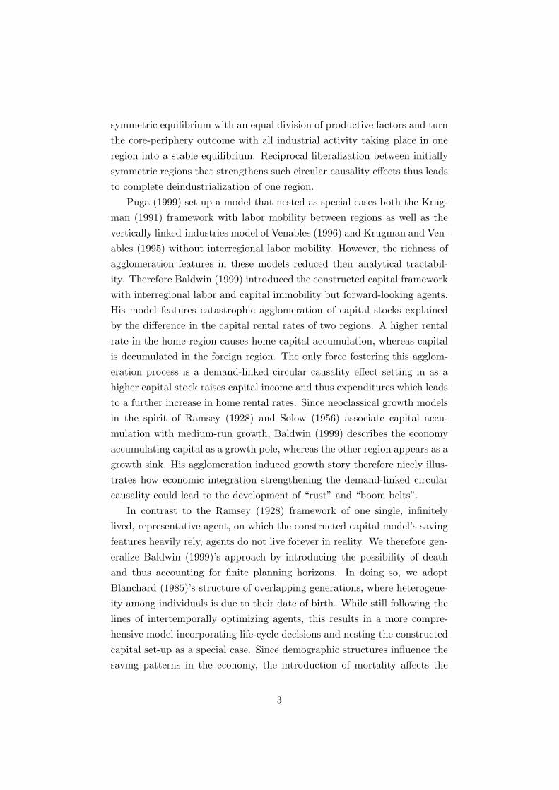
Figure 1 and 2 reveal that for these parameter ranges the derivativeof Esym with respect to µ is positive, whereas the derivative of Ksym isnegative.22 Consequently, a decrease in the mortality rate increases theaggregate equilibrium capital stock and decreases aggregate equilibrium ex-penditures. We can thus conclude that the mortality rate influences expen-ditures primarily via its positive effect on the discount rate. The savingbehavior channel dominates the population structure one capturing the ef-
21Recall, however, that production of the agricultural good in both regions requires ξto be sufficiently small (see section 2.4.1).
22We also investigated the derivatives for varying mortality rates. Assuming 0.008 ≤µ ≤ 0.025 resulting in a life expectancy between 40 and 120 years, and still consideringthe values for the other parameters mentioned before, does not change our findings.
18
Figure 2: Derivative of Ksym with respect to µ
fects of the mortality rate on the age composition of the population andexerting its influence via the heterogeneity of expenditure and wealth lev-els with respect to age. The positive dependence of aggregate equilibriumexpenditures on the mortality rate is fully consistent with the life cycle sav-ings literature claiming that longer planning horizons, i.e. lower mortalityrates, lead to higher individual savings and lower consumption levels (seee.g. Gertler (1999), Futagami and Nakajima (2001) or Zhang et al. (2003)).
As it turns out, when considering the impact of the mortality rate onthe steady-state consumption expenditure share23, Esym
δKsym+Esym, even ana-
lytical results can be derived. This share is obtainable from the ratio of theequilibrium capital stock to the equilibrium expenditures24
Ksym
Esym=
2ξF (δσ + ρσ +
√σ√σ(δ + ρ)2 + 4µ(µ+ ρ)ξ)
, (29)
23This share is defined as equilibrium consumption expenditures divided by steady-stateincome, where steady-state income is the sum of replacement investment, δK (equal tosavings in steady-state), and consumption expenditures.
24Simply calculate 1δKsymEsym
+1.
19

which obviously depends negatively on the mortality rate. Consistent withour numerical findings, a higher mortality rate thus increases the steady-state consumption expenditure share which again supports the predominantrole of the saving behavior channel.
4 Symmetric equilibrium stability -
The impact of introducing mortality on agglom-
eration
New Economic Geography models emphasize that reciprocal liberalizationbetween initially symmetric regions leads to catastrophic agglomeration, i.e.their main focus is on the instability of the symmetric equilibrium to be ableto explain agglomeration processes between regions. In this section we showthat the introduction of mortality considerably reduces the possibility of thesymmetric equilibrium to be unstable. As a consequence, agglomeration ofeconomic activity may not set in even if economic integration is promotedup to a high degree.
4.1 Formal stability analysis
The stability properties of the symmetric long-run equilibrium for varyingtrade costs and mortality rates are analyzed by following the classical ap-proach (see Barro and Sala-i-Martin (2004)) of linearizing the non-lineardynamic system given in equations (23), (24), (25) and (26) around thesymmetric equilibrium and then by evaluating the eigenvalues of the corre-sponding 4× 4 Jacobian matrix
Jsym =
(J1 J2
J3 J4
), (30)
where the four symmetric 2 × 2 sub-matrices Ji for i = 1, . . . , 4 are givenin appendix D. Solving the characteristic equation yields the following four
20
eigenvalues
eig1 =12
(r1 −√rad1), (31)
eig2 =12
(r1 +√rad1), (32)
eig3 =1
(φ+ 1)2√σ
(r2 −√rad2), (33)
eig4 =1
(φ+ 1)2√σ
(r2 +√rad2), (34)
where
r1 ≡ A√σ− δ,
rad1 ≡(A√σ
+ δ
)2
+(σ − ξ)
((A+B)2 + 4µ(µ+ ρ)ξ
)σξ
,
r2 ≡ 3φA+A−√σ(δ(2φ2 + φ+ 1
)+ (φ− 1)φρ
),
rad2 ≡(A(φ− 1) + (δ(φ− 1) + φ(φ+ 3)ρ)
√σ)2 +
(φ+ 1)(φσ + σ + φξ − ξ)((A+B)2(φ− 1)2 + 4µ(φ+ 1)2(µ+ ρ)ξ
)ξ
,
with the parameter clusters A ≡√σ(δ + ρ)2 + 4µ(µ+ ρ)ξ as well as B ≡
(δ + ρ)√σ. The signs and nature of these eigenvalues fully characterize the
system’s local dynamics around the symmetric equilibrium. Analyticallyinvestigating them25 thus results in lemma 1.
Lemma 1. Eigenvalue 3 is decisive for the local stability properties of thesymmetric equilibrium. A positive eigenvalue 3 implies instability, a negativeone saddle path stability.
Proof. By investigating the expressions for the eigenvalues it is first easilyestablished that all of them are real. This holds since both rad1 and rad2 arenonnegative for all possible parameter values (in particular since σ > ξ).26
Convergence to or divergence from the symmetric equilibrium is thereforemonotonic.
As there are two jump variables E and E∗, saddle path stability prevails25In order to get a first idea about the signs and nature of the eigenvalues, we also
calibrated the model and investigated the eigenvalues numerically. The correspondingfindings are presented in appendix D.
26Recall the parameter ranges σ > 1, 0 < δ ≤ 1, ρ > 0, 0 < µ ≤ 1, 0 < ξ < 1 and0 ≤ φ ≤ 1 which imply that A > 0 and B > 0.
21

if and only if there are two negative eigenvalues. If fewer than two eigenval-ues are negative, the system is locally unstable. By inserting the expressionfor A, it turns out that r1 > 0. We can thus immediately conclude thateigenvalue 2 is positive. In order to find out the sign of eigenvalue 1, wecompare r1 with the corresponding part under the radical, i.e. rad1. Thesquare of the former is smaller than the latter, implying that eigenvalue 1 isalways negative. It remains to investigate the signs of eigenvalues 3 and 4.Again we first check whether r2 is nonnegative. By inserting the expressionfor A, r2 can be rewritten as
r2 = −√σδ(2φ2 + φ+ 1
)︸ ︷︷ ︸term1
+√σ(1− φ)φρ︸ ︷︷ ︸term2
+
(1 + 3φ)√σ(δ + ρ)2 + 4µ(µ+ ρ)ξ︸ ︷︷ ︸
term3
. (35)
All three terms are increasing in ρ, ξ and µ but react differently to changesin φ, δ and σ. In order to show that r2 is nevertheless nonnegative for allparameter values we set ρ, ξ and µ equal to zero resulting in the “worst”, i.e.most negative, outcome with respect to these parameters. Since even in thiscase it is easily established that r2 is nonnegative for the whole feasible pa-rameter space the fourth eigenvalue is definitely positive. Summarizing, wehave shown that eigenvalue 2 and 4 are always positive, whereas eigenvalue1 is always negative. This proves the crucial role of the third eigenvalue asclaimed in lemma 1.
Having demonstrated that changes in the parameter values, and in par-ticular of the mortality rate, can only influence the stability properties ofthe symmetric equilibrium via eigenvalue 3, it is immediate to investigatethis eigenvalue more thoroughly. Figure 3 plots eigenvalue 3 as a functionof φ for three different mortality rates given our choice of the most plausiblevalues of the other parameters (ρ = 0.015, δ = 0.05, ξ = 0.3 and σ = 4).The graph indicates that, depending on the level of trade costs, eigenvalue 3switches its sign.27 Moreover, it is clearly visible that the range of φ withinwhich eigenvalue 3 is positive, crucially depends on the mortality rate. Thisobservation is investigated in the following proposition.
27The numerical investigation of eigenvalue 3 in appendix D also reveals that it isimpossible to come up with a definite sign for the whole parameter space.
22

Figure 3: Eigenvalue 3 as a function of φ for µ = 0 (dashed line),µ = 0.0002 (solid line) and µ = 0.0004 (dotted line)
Proposition 1. The sign of eigenvalue 3 and hence the stability propertiesof the symmetric equilibrium depend on the mortality rate.
Proof. To prove this proposition, we use the concept of the critical levelof trade costs φbreak. This threshold value identifies the degree of opennesswhere eigenvalue 3 changes its sign and therefore where the stability proper-ties of the symmetric equilibrium change (i.e. where eigenvalue 3 crosses thehorizontal axis in figure 3). To analytically obtain φbreak, we set the expres-sion for the third eigenvalue equal to zero and solve the resulting equation.This yields two solutions for φbreak as functions of the other parameters.28
Since these two critical levels in particular also depend on the mortality rate(see again figure 3 for a graphical illustration), proposition 1 holds.
So far, we have shown that changes in the mortality rate influence thestability properties of the symmetric equilibrium. Figure 3 moreover alreadyindicates the particular direction of the impact by illustrating that eigen-value 3 decreases in the mortality rate. The next section is dedicated toinvestigating this relationship between aging and the stability properties ofthe symmetric equilibrium in more detail.
28As the expressions are rather cumbersome they are not presented here but availableupon request.
23
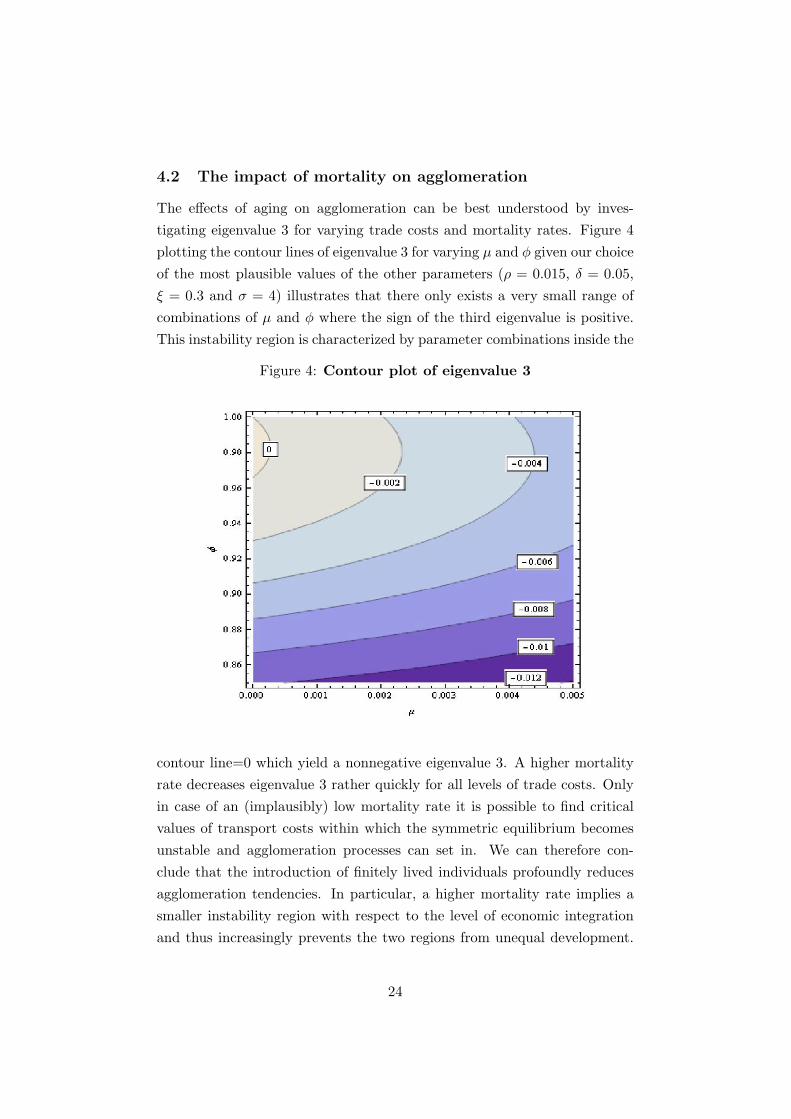
4.2 The impact of mortality on agglomeration
The effects of aging on agglomeration can be best understood by inves-tigating eigenvalue 3 for varying trade costs and mortality rates. Figure 4plotting the contour lines of eigenvalue 3 for varying µ and φ given our choiceof the most plausible values of the other parameters (ρ = 0.015, δ = 0.05,ξ = 0.3 and σ = 4) illustrates that there only exists a very small range ofcombinations of µ and φ where the sign of the third eigenvalue is positive.This instability region is characterized by parameter combinations inside the
Figure 4: Contour plot of eigenvalue 3
contour line=0 which yield a nonnegative eigenvalue 3. A higher mortalityrate decreases eigenvalue 3 rather quickly for all levels of trade costs. Onlyin case of an (implausibly) low mortality rate it is possible to find criticalvalues of transport costs within which the symmetric equilibrium becomesunstable and agglomeration processes can set in. We can therefore con-clude that the introduction of finitely lived individuals profoundly reducesagglomeration tendencies. In particular, a higher mortality rate implies asmaller instability region with respect to the level of economic integrationand thus increasingly prevents the two regions from unequal development.
24

The “smallness” of the instability region29 moreover implies that, in sharpcontrast to other New Economic Geography frameworks and in particular toBaldwin (1999)’s catastrophic agglomeration result, our model predicts thesymmetric outcome to be predominant even in the presence of high economicintegration.
The effects of aging on agglomeration are confirmed by investigating howthe critical levels of trade costs react to changes in the mortality rate. With-out mortality, i.e. µ = 0, and again applying our choice of the most plausibleparameter values, the two critical levels of trade costs are φbreak1 = 0.965974and φbreak2 = 1.30 In between those values, i.e. for sufficiently low levelsof trade costs, the symmetric equilibrium is unstable and agglomerationprocesses do set in. Allowing µ to increase, however, shows that φbreak1
increases, while φbreak2 decreases. The range of trade cost levels withinwhich the symmetric equilibrium is unstable clearly shrinks (in figure 3 thisshrinkage is equivalently represented by the downward shift of eigenvalue 3).Figure 5 illustrates this finding by plotting the the two critical levels of tradecosts for varying mortality rates as boundaries of the shaded instability re-gion. In particular, we can establish that for µ = 0.00028, corresponding to alife expectancy of less than approximately 3500 years, there exists no level oftrade costs such that the symmetric equilibrium is unstable (i.e. the down-ward shift in figure 3 is such that eigenvalue 3 does not cross the horizontalaxis anymore where it would become positive).31 Assuming reasonable val-ues of the mortality rate therefore implies that, again in sharp contrast toother New Economic Geography models, deeper economic integration doesnot result in agglomeration processes. We can thus also conclude that Bald-win (1999)’s agglomeration induced growth finding primarily applies in thevery special case of infinitely lived individuals.
Figure 5 does not only show that the instability region shrinks in the29Note that we plot this figure only for µ ≤ 0.005 and φ ≥ 0.85 which indicates how
small the instability region relative to the whole parameter range is.30When calibrating our model with the parameter values assumed by Baldwin (1999),
i.e. ρ = δ = 0.1, ξ = 0.3 and σ = 2, the two critical levels of trade costs exactly coincidewith Baldwin (1999)’s and are given by φbreak1 = 0.860465 and φbreak2 = 1.
31We also performed these simulations with respect to the critical level of trade costs forother parameter ranges, in particular for Baldwin (1999)’s parameter choice ρ = δ = 0.1,ξ = 0.3 and σ = 2. In this case the critical mortality rate, above which the symmetricequilibrium is always stable, is given by µ > 0.00395. This implies that in Baldwin (1999)’ssetup a life expectancy of less than approximately 250 years prevents any agglomerativetendencies.
25

Figure 5: φbreak1 (dashed) and φbreak2 (solid) as a function of µ
mortality rate but also reveals an interesting feature of the instability setwith respect to the level of trade costs: for low but positive mortality rates,the instability set is non-monotone in φ implying that agglomeration pro-cesses only set in for an intermediate range of trade costs and that thesymmetric equilibrium gets stable again for sufficiently high levels of eco-nomic integration. This is reflected by φbreak2 being smaller than one whichcontrasts with Baldwin (1999)’s set-up where φbreak2 is always equal to oneand the symmetric equilibrium is thus unstable for all values of φ beyondφbreak1 (see figure 5 for µ=0).32 The reason for this distinctive feature ofthe instability region becomes clear in the next section when looking at theforces weakening or fostering agglomeration in our model. As it turns out,such informal stability will moreover be useful for developing some economicintuition about the relationship between aging and agglomeration, i.e. forunderstanding the channel through which the mortality rate impacts uponthe stability properties of the symmetric equilibrium.
4.3 Economic intuition
As shown by Baldwin (1999), the formal stability analysis pursued in section4.1 yields the same results as a more informal way of checking the stability
32Figure 3 also illustrates that eigenvalue 3 is positive for all φ > φbreak1 in the case ofµ = 0.
26

of the symmetric equilibrium. This informal way is based on investigatinghow an exogenous perturbation of the home share of capital, θK , influencesthe profitability of home-based firms relative to foreign-based firms. A pos-itive impact implies instability as even more firms would locate in the homeregion, i.e. capital accumulation would set in.
We can isolate three channels via which production shifting influences therelative profitability of home-based firms. First, there is a pro-agglomerativedemand-linked circular causality effect. A higher capital share increases cap-ital income in the home region and thus its expenditure share. The associ-ated increased market size positively affects home profitability (see section2.4.2) and therefore causes further production shifting.33 The second chan-nel is based on the anti-agglomerative local competition effect capturing thenegative impact of production shifting upon equilibrium profits due to themore severe competition among home-based firms (see again section 2.4.2).Both these forces are present in Baldwin (1999)’s constructed capital modeland explain why agglomeration in this framework sets in for sufficiently highlevels of economic integration.
In our model, there appears, however, an additional dispersion forcestrengthening the stability of the symmetric equilibrium. In particular, theintroduction of finite planning horizons motivates the anti-agglomerativeturnover effect as a third channel via which production shifting changesthe profitability of home-based firms. This dispersion force is based on thedistributional effects caused by the turnover of generations. An exogenousrise in the home capital share increases wealth and thus expenditure levelsof individuals being currently alive in the home region relative to foreign-based individuals. The negative distributional effects on aggregate expen-ditures resulting from death, i.e. the replacement of these individuals bynewborns whose consumption expenditures are lower since they have zerowealth levels (see section 2.3), are thus more pronounced in the home re-gion. This, in turn, decreases the home expenditure share and thereforerelative profitability. Since a higher mortality rate increases the strength of
33This agglomeration force was first introduced by Baldwin (1999) and is due to theendogeneity of capital in his model. It hinges critically on the immobility of capital asonly in this case capital income cannot be repatriated to its immobile owners and thereforeincreases the region’s own income. In our model with capital immobility it is, however,indeed the case that the equilibrium value of the consumption expenditure share depends,via this income effect, on the capital stock.
27

the anti-agglomerative turnover effect, this third channel intuitively explainsthe positive impact of µ on the stability of the symmetric equilibrium. Wecan thus conclude that generalizing the constructed capital model to allowfor aging introduces an additional dispersion force that crucially depends onthe heterogeneity of individuals with respect to their expenditure and wealthlevels: as long as the consumption expenditures of newborns are smaller thanaverage consumption expenditures, the turnover effect is active and the as-sociated distributional effects due to death work against agglomeration.
Going back to figure 5, we are now able to explain the non-monotonicityof the instability set with respect to the level of trade costs. From figure3 it is evident that the relative strength of the agglomeration force, as rep-resented by eigenvalue 3, is maximized for φ < 1. This is also the case forBaldwin (1999)’s set-up with a zero mortality rate. In particular, both thelocal competition and the agglomeration force present in the constructedcapital model decrease in the level of trade costs. The local competitioneffect diminishes since freer trade makes firms less dependent on the homemarket, whereas the demand-linked circular causality effect is reduced aslocal sales increasingly lose importance. Both forces, however, diminish atdifferent speeds with the competition force being reduced more rapidly forhigh levels of trade costs whereas the decrease of the agglomeration force isstronger for sufficiently low levels of trade barriers. This implies that the rel-ative strength of the agglomeration force is largest for an intermediate levelof trade costs. Since eigenvalue 3 remains positive and the symmetric equi-librium thus unstable for all φ > φbreak1 (see eigenvalue 3 for µ = 0 in figure3), this special feature does not have any consequences for the instabilityset in the case of a zero mortality rate. The introduction of finite horizons,however, additionally decreases eigenvalue 3 for all levels of trade costs dueto the anti-agglomerative turnover effect. For µ > 0, the non-monotonicityof the relative strength of the agglomeration force therefore qualitativelychanges the stability properties of the symmetric equilibrium: as shown infigure 5, φbreak1 increases and φbreak2 decreases below one implying that thesymmetric equilibrium retains its stability for sufficiently high levels of tradeopenness. The emergence of an additional dispersion force, when allowingfor finite planning horizons, thus explains the non-monotonicity of the in-stability set with respect to the level of economic integration in the case ofa positive mortality rate.
28

5 Concluding remarks
The model in this paper introduces demography into the New EconomicGeography by generalizing the constructed capital framework of Baldwin(1999) to account for changes in the age structure of the population. In-corporating finite individual planning horizons allows us to investigate theimpacts of population aging on agglomeration tendencies of economic activ-ities. We show that the introduction of mortality stabilizes the symmetricequilibrium and thus acts as a force that promotes a more equal distributionof productive factors between two regions.
From the point of view of economic policy, we can conclude that, in sharpcontrast to other New Economic Geography approaches, our model does notnecessarily associate sufficiently deep integration with high interregional in-equality. In particular, we have shown that plausible mortality rates are faraway from supporting agglomeration processes. Consequently, there is noneed to impose any type of trade barriers in order to avoid deindustrializa-tion of one region resulting from decreased transport costs. Especially in thecase of the European Union this implies that there is no tradeoff between itstwo most important targets: integration on the one hand and interregionalequality on the other hand. Instead, the implementation of appropriate poli-cies to achieve one objective does not interfere with the realization of theother goal.
However, introducing mortality was only a first step towards a morecomprehensive understanding of the interrelations between aging, economicintegration and agglomeration. The assumption of a constant mortality rateadopted for the sake of analytical tractability is still at odds with reality.Using age dependent mortality rates is therefore one possible line for futureresearch. Similarly, investigating the effects of age dependent labor produc-tivity on agglomeration processes might yield important insights, especiallywhen viewing labor productivity as decisive for a region’s competitiveness.Moreover, it would be worthwhile to consider asymmetric regions, in partic-ular with respect to mortality. In such a setting one could investigate howdifferences in mortality rates are linked to differences in capital accumulationrates, again a question of high relevance for economic policy.
29

Acknowledgements
We thank Dalkhat Ediev (Vienna Institute of Demography), Ingrid Ku-bin (Vienna University of Economics and Business Administration), AlexiaPrskawetz (Vienna University of Technology), Gerhard Orosel (Universityof Vienna), Gerhard Sorger (University of Vienna), Jens Sudekum (Univer-sity of Duisburg-Essen), Vladimir Veliov (Vienna University of Technology),Stefan Wrzaczek (Vienna University of Technology), and the conference par-ticipants at the RIEF Doctoral Meeting 2009 and at the Annual Meeting ofthe Austrian Economic Association 2009 as well as the seminar participantsat the Institute for Advanced Studies, the University of Vienna, the ViennaUniversity of Economics and Business and the Vienna Institute for Interna-tional Economics Studies for helpful comments and suggestions. The paperwas prepared within the research project “Agglomeration processes in agingsocieties” funded by the Vienna Science and Technology Fund (WWTF) inits “Mathematics and... Call” 2007.
30

Appendix
A The individual’s utility optimization problem
Suppressing time arguments in the optimization procedure, the current valueHamiltonian for the individual’s optimization problem is
H(e, k, λ, t) = ln[ eP
]+ λ
(wl + πk − e
wF+ µk − δk
)(36)
where P is the perfect price index translating expenditures into indirectutility.34 The first order conditions of the problem associated with equation(36) are given by
∂H
∂e
!= 0 ⇒ 1e
=λ
Fw, (37)
∂H
∂k
!= (ρ+ µ)λ− λ ⇒ λ
λ= − π
Fw+ ρ+ δ, (38)
∂H
∂λ
!= k ⇒ wl + πk − ewF
+ µk − δk = k (39)
and the standard transversality condition. Taking the time derivative ofequation (37) under the assumption that w is time independent35 and com-bining it with equation (38) yields the individual consumption Euler equa-tion
e
e=
π
Fw− δ − ρ.
The static problem of dividing consumption between the manufacturingcomposite and the agricultural good for fixed consumption expenditure ecan be formulated as
maxcaggm ,cn
(cn)1−ξ(caggm )ξ
s.t. pncn + paggm caggm = e, (40)
where paggm is an appropriate price index which can be shown to equal aweighted average of the two Dixit and Stiglitz (1977) price indexes at homeand foreign with the foreign price index being augmented by transport costs.
34This price index can be obtained from the solution to the optimization problem instage two and three.
35Section 2.4.1 shows that this indeed holds as the wage rate is pinned down by theprice of the agricultural good which is chosen to be the numeraire of the economy.
31

Setting up the Lagrangian
`(cn, caggm , λa) = (cn)1−ξ(caggm )ξ + λa (e− pncn − paggm caggm ) (41)
and solving for the first order conditions yields
∂`
∂cn
!= 0 ⇒ (1− ξ)(cn)−ξ(caggm )ξ = λapn, (42)
∂`
∂caggm
!= 0 ⇒ (cn)1−ξξ(caggm )ξ−1 = λapaggm , (43)
∂`
∂λa
!= 0 ⇒ pncn + paggm caggm = e. (44)
Manipulating these first order conditions leads to unit elastic demands forthe agricultural good and the CES composite of manufactured varieties givenby
cn =(1− ξ)epn
caggm =ξe
paggm. (45)
Due to the Cobb-Douglas specification of utility, a fraction ξ of incomeused for consumption is spent on manufactures and a fraction 1− ξ on theagricultural good.
In the last stage, the static problem of distributing manufacturing con-sumption among different varieties for fixed manufacturing consumption ex-penditure ξe can be formulated as
maxcHm(i),cFm(j)
[∫ VH
0
(cHm(i)
)σ−1σ di+
∫ VF
0
(cFm(j)
)σ−1σ dj
] σσ−1
s.t.∫ VH
0pHm(i)cHm(i)di+
∫ VF
0pFm,ϕ(j)cFm(j)dj = ξe. (46)
Setting up the Lagrangian
`(cHm(i), cFm(j), λm) =
[∫ VH
0
(cHm(i)
)σ−1σ di+
∫ VF
0
(cFm(j)
)σ−1σ dj
] σσ−1
+
λm
[ξe−
∫ VH
0
pHm(i)cHm(i)di−∫ VF
0
pFm,ϕ(j)cFm(j)dj
](47)
32

and solving for the first order conditions yields36
∂`
∂cHm(i)!= 0 ⇒ σ
σ − 1
[∫ VH
0(cHm(i))
σ−1σ di+
∫ VF
0(cFm(j))
σ−1σ dj
] 1σ−1
×σ − 1σ
(cHm(i))−1σ = λmp
Hm(i), (48)
∂`
∂cFm(j)!= 0 ⇒ σ
σ − 1
[∫ VH
0(cHm(i))
σ−1σ di+
∫ VF
0(cFm(j))
σ−1σ dj
] 1σ−1
×σ − 1σ
(cFm(j))−1σ = λmp
Fm,ϕ(j), (49)
∂`
∂λm
!= 0 ⇒∫ VH
0pHm(i)cHm(i)di+
∫ VF
0pFm,ϕ(j)cFm(j)dj = ξe. (50)
Recalling the definition of caggm given below equation (1), these first orderconditions can be rewritten as
caggm
[∫ VH
0(cHm(i))
σ−1σ di+
∫ VF
0(cFm(j))
σ−1σ dj
]−1
(cHm(i))−1σ = λmp
Hm(i),
(51)
caggm
[∫ VH
0(cHm(i))
σ−1σ di+
∫ VF
0(cFm(j))
σ−1σ dj
]−1
(cFm(j))−1σ = λmp
Fm,ϕ(j).
(52)
Isolating cHm(i) and cFm(j) on the left hand side, then multiplying both sidesby pHm(i) or pFm,ϕ(j) and finally integrating over all varieties yields
∫ VH
0pHm(i)cHm(i)di =
λ−σm∫ VH
0 (pHm(i))1−σdi[∫ VH
0 (cHm(i))σ−1σ di+
∫ VF0 (cFm(j))
σ−1σ dj
]−σ(caggm )−σ
,∫ VF
0pFm,ϕ(j)cFm(j)dj =
λ−σm∫ VF
0 (pFm,ϕ(j))1−σdj[∫ VH
0 (cHm(i))σ−1σ di+
∫ VF0 (cFm(j))
σ−1σ dj
]−σ(caggm )−σ
.
Adding these two expressions, using the budget constraint from above, and36Note that this is in fact a variational problem.
33

isolating λm gives the Lagrange multiplier
λm =(ξe)−
1σ caggm
[∫ VH0 (pHm(i))1−σdi+
∫ VF0 (pFm,ϕ(j))1−σdj
] 1σ[∫ VH
0 (cHm(i))σ−1σ di+
∫ VF0 (cFm(j))
σ−1σ dj
] , (53)
i.e. the shadow price of manufacturing consumption. Plugging this expres-sion back into equations (51) and (52) finally leads to the demands for allvarieties
cHm(i) =ξe(pHm(i))−σ[∫ VH
0 (pHm(i))1−σdi+∫ VF
0 (pFm,ϕ(j))1−σdj] ,
cFm(j) =ξe(pFm,ϕ(j))−σ[∫ VH
0 (pHm(i))1−σdi+∫ VF
0 (pFm,ϕ(j))1−σdj] .
B Aggregation over individuals
Following Heijdra and van der Ploeg (2002), chapter 16, the aggregate Eulerequation can be derived as follows. Taking the time derivative of aggregateconsumption expenditures defined in equation (9) yields
E(t) = µe(t, t) + µ
∫ t
−∞e(t0, t)e−µ(t−t0) + e(t0, t)(−µ)e−µ(t−t0)dt0
= µe(t, t)− µE(t) + µ
∫ t
−∞e(t0, t)e−µ(t−t0)dt0, (54)
where we used again the definition of aggregate consumption expendituresin going from the first to the second line. To arrive at the final aggregateEuler equation it is necessary to derive optimal consumption expenditurese(t, t) of newborns in the planning period t and the aggregate consumptionexpenditure rule E(t). To achieve this, we reformulate the individual’s op-timization problem as follows. In line with equation (1) the expected utilityU(t0, t) at an arbitrary point in time t of a consumer born at time t0 ≤ t isgiven by
U(t0, t) ≡∫ ∞t
e−(ρ+µ)(τ−t)ln
(e(t0, τ)P (τ)
)dτ, (55)
where we again used the perfect price index P translating expenditures inindirect utility (see appendix A). The law of motion of capital given in
34

equation (2) can be rewritten as
k(t0, τ) =w(τ)l(τ) + π(τ)k(t0, τ)− e(t0, τ)
w(τ)F+ µk(t0, τ)− δk(t0, τ)
=(
π(τ)w(τ)F
+ µ− δ)k(t0, τ) +
l(τ)F− e(t0, τ)w(τ)F
. (56)
From equation (56) the individual’s lifetime budget can be derived. First
both sides of the equation are multiplied by e−RA(t,τ) ≡ e
−∫ τt
(π(s)w(s)F
+µ−δ)ds
and rearranged to[k(t0, τ)−
(π(τ)w(τ)F
+ µ− δ)k(t0, τ)
]e−R
A(t,τ) =[l(τ)F− e(t0, τ)w(τ)F
]e−R
A(t,τ).
(57)
Observing that the left hand side of equation (57) is d[k(t0, τ)e−R
A(t,τ)]/dτ
by applying Leibnitz’s rule to recognize that dRA(t, τ)/dτ = π(τ)w(τ)F + µ− δ
and integrating over the interval [t,∞) yields∫ ∞t
d[k(t0, τ)e−R
A(t,τ)]
=∫ ∞t
[l(τ)F− e(t0, τ)w(τ)F
]e−R
A(t,τ)dτ.
This expression can be solved to
limτ→∞
k(t0, τ)e−RA(t,τ) − k(t0, t)e−R
A(t,t) = HW (t)−∫ ∞t
e(t0, τ)w(τ)F
e−RA(t,τ)dτ,
(58)where HW (t) ≡
∫∞t
w(τ)l(τ)w(τ)F e−R
A(t,τ)dτ denotes human wealth of individualsin capital units consisting of the present value of lifetime wage income usingthe annuity factor RA(t,τ) for discounting. Note that e−R
A(t,t) = 1 and thatthe first term on the left hand side represents “terminal capital holdings”.These holdings must be equal to zero because first, the insurance companywill ensure their nonnegativity, and second, it is suboptimal for an individualto have positive terminal assets as there is neither a bequest motive norsatiation from consumption. Taking this into account, yields the followingsolvency condition
limτ→∞
e−RA(t,τ)k(t0, τ) = 0, (59)
which prevents an individual from running a Ponzi game against the life-insurance company. The No-Ponzi-Game condition can be inserted in equa-
35

tion (58) to obtain the individual’s lifetime budget restriction
k(t0, t) +HW (t) =∫ ∞t
e(t0, τ)w(τ)F
e−RA(t,τ)dτ. (60)
The present value of an individual’s consumption expenditure plan in cap-ital units must be equal to the sum of human wealth in capital units andcapital holdings (=total wealth). Evaluating the lifetime budget constraintat t = t0 shows that the discounted sum of lifetime labor earnings mustequal discounted consumption expenditures.37 This implies, from investi-gating the law of motion for capital, that discounted savings are equal todiscounted accumulated profits, i.e. savings are only used for reallocatingconsumption across lifetime.
Maximizing expected utility given in equation (55) subject to the budgetconstraint in equation (60) yields the following first order condition
1e(t0, τ)
e−(ρ+µ)(τ−t) = λ(t)1
w(τ)Fe−R
A(t,τ), τ ∈ [t,∞), (61)
where λ(t) represents the marginal expected lifetime utility of wealth.38 In-dividuals should therefore plan consumption expenditures in a way such thatthe appropriately discounted marginal utility of expenditures and wealth areequated.
Applying equation (61) for the planning period (τ = t) yields e(t0, t) =w(t)Fλ(t) . Using this result and then substituting for λ(t) also from the first
order condition in equation (61) helps to establish the following equality∫ ∞t
e(t0, t)e−(ρ+µ)(τ−t)dτ =∫ ∞t
w(t)Fλ(t)
e−(ρ+µ)(τ−t)dτ
= Fw(t)∫ ∞t
e(t0, τ)Fw(τ)
e−RA(t,τ)dτ.
Integrating out and using the lifetime budget constraint of equation (60)37Recall that capital holdings of newborns k(t0, t0) are zero by assumption (no bequests).38Differentiating this first order condition with respect to τ , inserting the expression
for λ(t) also obtainable from this first order condition and simplifying yields the followingEuler equation
e(t0, τ)
e(t0, τ)=
π(τ)
w(τ)F− ρ− δ +
w(τ)
w(τ). (62)
With time-invariant wages (see section 2.4.1), this Euler equation is exactly the same asthe one obtained in equation (6).
36

finally yields consumption expenditures e(t0, t) in the planning period t
e(t0, t)ρ+ µ
[−e−(ρ+µ)(τ−t)
]∞t
= Fw(t)[k(t0, t) +HW (t)]
e(t0, t) = (ρ+ µ)Fw(t)[k(t0, t) +HW (t)]. (63)
The above equation clearly shows that optimal consumption expendituresin the planning period t in capital units, e(t0,t)
Fw(t) , are proportional to totalwealth with the marginal propensity to consume out of total wealth beingconstant and equal to the effective rate of time preference ρ+ µ.
Using this expression for optimal consumption expenditures in the def-inition of aggregate consumption expenditures in equation (9) yields thefollowing very simple aggregate consumption expenditure rule
E(t) ≡ µ
∫ t
−∞e−µ(t−t0)(ρ+ µ)Fw(t)[k(t0, t) +HW (t)]dt0
= (ρ+ µ)Fw(t)µ[∫ t
−∞e−µ(t−t0)k(t0, t)dt0 +
∫ t
−∞e−µ(t−t0)HW (t)dt0
]= (ρ+ µ)Fw(t) [K(t) +HW (t)] , (64)
where the aggregate capital stock is defined in equation (7) and can berewritten in analogy to aggregate consumption expenditures in equation (9).
Moreover it is easily established that µHW (t)[e−µ(t−t0)
µ
]t−∞
= HW (t).39
Finally we modify equation (54) by substituting for e(t, t) and E(t) fromthe derived expressions of equation (63) evaluated at birth date t40 andequation (64) as well as for e(t0, t) from the individual Euler equation given
39This aggregation property of consumption expenditures is due to the fact that weassume a constant probability of death implying an age independent marginal propensityto consume out of total wealth (see equation (63)).
40Note again that k(t, t) = 0 and newborns therefore consume a fraction of their humanwealth at birth, i.e. e(t, t) = (ρ+ µ)Fw(t)HW (t).
37

in expression (62). Dividing by E(t) then gives the aggregate Euler equation
E(t)E(t)
= −µ(ρ+ µ)Fw(t)K(t)E(t)
+
µ
E(t)
∫ t
−∞e(t0, t)
[π(t)w(t)F
− ρ− δ +w(t)w(t)
]e−µ(t−t0)dt0
= −µ(ρ+ µ)Fw(t)K(t)E(t)
+π(t)w(t)F
− ρ− δ +w(t)w(t)
= −µE(t)− e(t, t)E(t)
+e(t0, t)e(t0, t)
,
where in the third line we used again the definition of aggregate consumptionexpenditure from equation (9) and the term w(t)/w(t) disappears in the caseof time invariant wages (see section 2.4.1).
C The manufacturing firm’s profit maximization
problem - Derivation of rental rates
By substituting for optimal demands for varieties from the constraints ofthe maximization problem as stated in equation 18, operating profit can berewritten as
(pHm(i, t)− w(t)β)(∫ t
−∞
ξe(t0, t)(pHm(i, t))−σ
Pm(t)N(t0, t)dt0
)+
(pFm,ϕ(i, t)− w(t)ϕβ)
(∫ t
−∞
ξe∗(t0, t)(pFm,ϕ(i, t))−σ
P ∗m(t)N∗(t0, t)dt0
),
(65)
whose derivatives with respect to pHm(i, t) and pFm,ϕ(i, t) are set equal to zeroto yield the first order conditions∫ t
−∞ ξe(t0, t)N(t0, t)dt0Pm(t)
[(1− σ)(pHm(i, t))−σ + σw(t)β(pHm(i, t))−σ−1
]= 0,
∫ t−∞ ξe∗(t0, t)N∗(t0, t)dt0
P ∗m(t)[(1− σ)(pFm,ϕ(i, t))−σ + σw(t)βϕ(pFm,ϕ(i, t))−σ−1
]= 0.
38

Rearranging and simplifying gives optimal prices
pHm(i, t) =σ
σ − 1w(t)β,
pFm,ϕ(i, t) =σ
σ − 1w(t)βϕ.
Using these pricing rules and the definition of aggregate expenditures givenin equation 8 in equation 65 and simplifying yields operating profits as
π(t) =ξE(t)
σ(K(t) + ϕ1−σK∗(t))+
ξϕ1−σE∗(t)σ(ϕ1−σK(t) +K∗(t))
(66)
where an equivalent equation holds in the foreign region. Note that thenumber of varieties in the home region VH(t) is equal to the capital stockat home K(t) as one variety exactly requires one unit of capital as fixedinput (analogously K∗(t) ≡ VF (t)) and that the variety index i can bedropped since prices and therefore profits are equal for all firms. Applyingthe definitions of regional share variables and global quantities as well as thedefinition of openness yields the final expressions for regional rental rates41
π =(
θEθK + φ(1− θK)
+(1− θE)φ
φθK + 1− θK
)︸ ︷︷ ︸
Bias
(ξEW
σKW
),
π∗ =(
1− θE1− θK + φθK
+θEφ
φ(1− θK) + θK
)︸ ︷︷ ︸
Bias∗
(ξEW
σKW
).
41We ignore time arguments here.
39

D Intermediate results for the stability analysis
The Jacobian matrix Jsym, which is evaluated at the symmetric equilibriumand given in equation 30, has the following entries Ji for i = 1, . . . , 4:
J1 =1
2(φ+ 1)√σ
(A(φ+ 2)−Bφ (A+B)φ
(A+B)φ A(φ+ 2)−Bφ
), (67)
J2 =
−F (A+B)2(φ2+1)4(φ+1)2ξ − Fµ(µ+ ρ) − (A+B)2Fφ
2(φ+1)2ξ
− (A+B)2Fφ2(φ+1)2ξ
−F (A+B)2(φ2+1)4(φ+1)2ξ − Fµ(µ+ ρ)
,
(68)
J3 =1
F (φ+ 1)σ
(ξ − (φ+ 1)σ φξ
φξ ξ − (φ+ 1)σ
), (69)
J4 =
φ(A+ρ√σ)−δ(φ2+φ+1)√σ(φ+1)2
√σ
− (A+B)φ(φ+1)2
√σ
− (A+B)φ(φ+1)2
√σ
φ(A+ρ√σ)−δ(φ2+φ+1)√σ(φ+1)2
√σ
, (70)
with the parameter clusters A ≡√σ(δ + ρ)2 + 4µ(µ+ ρ)ξ as well as B ≡
(δ + ρ)√σ.
In order to get a first insight into the nature and signs of the eigenvaluesof Jsym, we calibrated the model using the parameter values ρ = 0.015 andδ = 0.05 and allowing the elasticity of substitution and the manufacturingshare of consumption to vary within the ranges 2 ≤ σ ≤ 8 and 0.1 ≤ ξ ≤ 0.9.Figures 6, 7, 8 and 9 illustrate the numerical investigation of the signs ofthe eigenvalues for σ = 4, ξ = 0.3 and varying µ and φ.42
First, the figures suggest that all eigenvalues are real for the chosen pa-rameter space. Moreover, figures 6, 7 and 9 show that the first eigenvalueis always negative, whereas the second and fourth are always positive. Thisresult is independent of the level of transport costs and the mortality rate.Saddle path stability of the symmetric equilibrium therefore seems to cru-cially depend on the third eigenvalue by requiring it to be negative. As canbe seen from the 3D plot in figure 8 there only exists a very small range ofcombinations of low µ and high φ where the sign of the third eigenvalue ispositive. One is therefore tempted to conclude that with a sufficiently highmortality rate, the symmetric equilibrium is stable for all levels of transportcosts.
42We also conducted the same simulations for other values of σ and ξ within the consid-ered range. Overall, we find that our findings with respect to the signs of the eigenvaluesare insensitive to changes in those parameters.
40

Figure 6: Eigenvalue 1
Figure 7: Eigenvalue 2
41

Figure 8: Eigenvalue 3
Figure 9: Eigenvalue 4
42

References
Auerbach, A. J. and Kotlikoff, L. J. (1987). Dynamic Fiscal Policy. Cam-bridge University Press.
Baldwin, R., Forslid, R., Martin, P., Ottaviano, G., and Robert-Nicoud, F.(2003). Economic Geography & Public Policy. Princeton University Press.
Baldwin, R. E. (1999). Agglomeration and endogenous capital. EuropeanEconomic Review, Vol. 43(No. 2):253–280.
Barro, R. J. and Sala-i-Martin, X. S. (2004). Economic Growth. MIT Press.
Blanchard, O. J. (1985). Debt, deficits and finite horizons. Journal ofPolitical Economy, Vol. 93(No. 2):223–247.
Bosker, M. and Garretsen, H. (2007). Trade costs, market access and eco-nomic geography: Why the empirical specification of trade costs matters.CEPR Discussion Paper 2071, pages 1–41.
Brakman, S., Garretsen, H., and Schramm, M. (2005). Putting the neweconomic geography to the test: Free-ness of trade and agglomeration inthe EU regions. CESifo Working Paper No. 1566, pages 1–38.
Dixit, A. K. and Stiglitz, J. E. (1977). Monopolistic competition and opti-mum product diversity. American Economic Review, Vol. 67(No. 3):297–308.
Eurostat (2004). Eurostat yearbook 2004: The statistical guide to Europe.Office for Official Publications of the European Communities.
Futagami, K. and Nakajima, T. (2001). Population aging and economicgrowth. Journal of Macroeconomics, Vol. 23(No. 1):31–44.
Gertler, M. (1999). Government debt and social security in a life-cycleeconomy. Carnegie-Rochester Conference Series on Public Policy, Vol.50:61–110.
Head, K. and Mayer, T. (2003). The empirics of agglomeration and trade.CEPII Working Papers, pages 1–69.
Heijdra, B. J. and van der Ploeg, F. (2002). Foundations of Modern Macroe-conomics. Oxford University Press.
43

Krugman, P. (1991). Increasing returns and economic geography. Journalof Political Economy, Vol. 99(No. 3):483–499.
Krugman, P. and Venables, A. J. (1995). Globalization and the inequality ofnations. The Quarterly Journal of Economics, Vol. 110(No. 4):857–880.
Martin, P. and Ottaviano, G. (1999). Growing locations: Industry loca-tion in a model of endogenous growth. European Economic Review, Vol.43:281–302.
Puga, D. (1999). The rise and fall of regional inequalities. European Eco-nomic Review, Vol. 43:303–334.
Ramsey, F. P. (1928). A mathematical theory of saving. The EconomicJournal, Vol. 38(No. 152):543–559.
Sachs, J. D. and Warner, A. (1995). Economic reform and the process ofglobal integration. Brookings Papers on Economic Activity, (No. 1):1–118.
Solow, R. M. (1956). A contribution to the theory of economic growth. TheQuarterly Journal of Economics, Vol. 70(No. 1):65–94.
United Nations (2007). World population prospects: The 2006 revision. Url:http://www.un.org/esa/population/publications/wpp2006/english.pdf.
Venables, A. J. (1996). Equilibrium locations of vertically linked industries.International Economic Review, Vol. 37(No. 2):341–359.
Yaari, M. E. (1965). Uncertain lifetime, life insurance and the theory of theconsumer. The Review of Economic Studies, Vol. 32(No. 2):137–150.
Zhang, J., Zhang, J., and Lee, R. (2003). Rising longevity, education, sav-ings, and growth. Journal of Development Economics, Vol. 70(No. 1):83–101.
44