Ups

Qa

b

c

I

a

ARRAA

KMMPS

1

senbs1foHfto

h0

Agricultural and Forest Meteorology 232 (2017) 606–622

Contents lists available at ScienceDirect

Agricultural and Forest Meteorology

j o ur na l ho me pag e: www.elsev ier .com/ locate /agr formet

sing the particle swarm optimization algorithm to calibrate thearameters relating to the turbulent flux in the surface layer in theource region of the Yellow River

idong Yanga,∗, Jian Wua, Yueqing Lib, Weidong Lia, Lijuan Wangc, Yang Yangc

Department of Atmospheric Sciences, Yunnan University, Yunnan Province 650091, ChinaInstitute of Plateau Meteorology, China Meteorological Administration, Sichuan Province 610000, ChinaGansu Key Laboratory of Arid Climatic Change and Reducing Disater/Key Open Laboratory of Arid Climatic Change and Disaster Reduction of CMA,

nstitute of Arid Meteorology, China Meteorological Administration, Gansu Province 730020, China

r t i c l e i n f o

rticle history:eceived 10 March 2016eceived in revised form 18 October 2016ccepted 24 October 2016vailable online 28 October 2016

eywords:aqu stationonin-Obukhov similarity theory

a b s t r a c t

Accurately determining the fluxes of mass and energy between land and the atmosphere is important forunderstanding regional climates and hydrological cycles. In numerical modeling, the parameterization ofa turbulent flux is usually based on Monin-Obukhov similarity theory (MOST). According to this theory,it is necessary to simultaneously calculate the empirical similarity parameters ˇm, ˇh, �m, and �h, theaerodynamic roughness (z0m) and the thermal roughness (zT ). However, it is difficult to solve a simulta-neous set of nonlinear equations for these six parameters. In this study, a new method was introduced tosolving this problem. Using measurements from Maqu Station in the source region of the Yellow River,this study employed the artificial intelligence particle swarm optimization (PSO) algorithm to calibrate

article swarm optimization algorithmource region of the Yellow River

the parameters relating to the turbulent flux in the surface layer. We concluded that the differences inthe sensible heat and momentum fluxes between the calculations that used the calibrated parametersand the measurements were rather small and that their correlation coefficients were relatively high. Theresults suggested that PSO algorithm is a feasible approach which can be applied in MOST parameterestimation.

© 2016 The Author(s). Published by Elsevier B.V. This is an open access article under the CC BY license

. Introduction

The atmospheric surface layer is at the bottom of the atmo-pheric boundary layer. Due to the strong aerodynamic and thermalffects of the underlying surface, atmospheric motion is domi-ated by turbulence. The mass and energy exchanges that occuretween the atmosphere and land surface via turbulent fluxesignificantly impact both weather and climate (Dickinson et al.,998; Seneviratne et al., 2006). In numerical modeling, schemesor parameterizing the turbulent surface flux enforce the balancesf mass and energy between land and the atmosphere (Beljaars andoltslag, 1991; Chen et al., 1997; Garratt and Pielke, 1989). There-

ore, to improve the performance of climate models, it is important

o carefully study the physical interactions between different typesf land surface and the atmosphere, develop optimal schemes for

∗ Corresponding author.E-mail address: yangqd@ynu.edu.cn (Q. Yang).

ttp://dx.doi.org/10.1016/j.agrformet.2016.10.019168-1923/© 2016 The Author(s). Published by Elsevier B.V. This is an open access article

(http://creativecommons.org/licenses/by/4.0/).

parameterizing the turbulent fluxes and accurately determine theland-atmosphere fluxes of mass and energy.

In global climate models, the land-atmosphere fluxes ofmomentum, sensible heat and water vapor are usually calculatedusing the wind velocity, potential temperature and humidity gra-dients with the relevant bulk transfer coefficients (Dai, 2003; Niu,2011; Zeng and Dickinson, 1998). The wind velocity, potentialtemperature and humidity gradients can be directly measured.Therefore, accurately determining the bulk transfer coefficients isthe key to parameterizing the turbulent fluxes in numerical models.Since the Monin-Obukhov similarity theory (MOST) was proposedin the 1950s (Dyer, 1974; Monin and Obukhov, 1954), significantbreakthroughs have been made in the parameterization of surfaceturbulent fluxes (Businger et al., 1971; Dyer, 1974). More than 20parameterization schemes for the bulk transfer coefficients havebeen developed based on this theory (Abdella and McFarlane, 1996;Łobocki, 1993; Louis, 1979; Paulson, 1970), and these schemes have

been widely applied in various types of numerical model. Accord-

under the CC BY license (http://creativecommons.org/licenses/by/4.0/).

rest M

ir

C

C

wtKfhsr

h1f(vmt

�

�

wfaebI�ftpm

a(ssabbMarlwfta(tctt2

Q. Yang et al. / Agricultural and Fo

ng to MOST, the land-atmosphere bulk transfer coefficients can beepresented as follows:

D = �2

[ln(z/z0m) − m(z/L)

]2(1)

H = CE = �2[ln(z/z0m) − m(z/L)

] [ln(z/zT ) − h(z/L)

] (2)

here CD , CH and CE are the bulk transfer coefficients of momen-um, sensible heat and water vapor, respectively, � is the vonarman constant. �M and �H are the integrals of the similarity

unctions associated with momentum and heat. z is a referenceeight, L is the Obukhov length, z/L represents the atmospherictability, z0m is the aerodynamic roughness and zT is the thermaloughness.

Many studies of the similarity functions in the above equationsave been conducted (Businger et al., 1971; Dyer, 1974; Högström,996). Near-surface measurements with different underlying sur-ace types were found to lead to different forms of these functionsvan den Hurk and Holtslag, 1997). Sorbjan (1986) reviewed pre-ious results and summarized the similarity functions for theomentum and sensible heat as follows, based on the status of

he atmospheric stability (Sorbjan, 1986):

m =

⎧⎨⎩

1 + ˇm(z

L)z

L≥ 0

−1/4 z

L< 0

(3)

h =

⎧⎨⎩

1 + ˇhz

L

z

L≥ 0

−1/2 z

L< 0

(4)

here ϕm and ϕh are the differential expressions of the similarityunctions, ˇm and ˇh, and �m and �h are empirical parameters thatre normally regressed from measurements. In numerical mod-ls, the similarity functions obtained by Businger and Dyer haveeen most widely used (Dai, 2003; Niu, 2011; Oleson et al., 2010).n these functions, the empirical parameters are ˇm = ˇh = 16 andm = �h = 4.7. However, these functions are not always suitable

or all seasons and surface types. Numerous studies have shownhat the selection of empirical parameters depends largely on thehysical properties of the underlying surface, the accuracy of theeasurements and the methods of the study (Högström, 1988).The stability parameter z/L determines the atmosphere’s motion

nd thermal status. It is usually an implicit function of C Yang et al.2001) suggested that z/L can be represented by the bulk Richard-on number and similarity functions (Yang et al., 2001). Undertable conditions, because the similarity functions are linear, annalytical solution for z/L is available. In contrast, under unsta-le conditions, the similarity functions are nonlinear, and z/L cane obtained via iteration or semi-analytical methods (Abdella andcFarlane, 1996; Łobocki, 1993; Louis, 1979; Paulson, 1970; Sharan

nd Srivastava, 2014). The atmosphere aerodynamic and thermaloughness lengths are two parameters that are important for calcu-ating the bulk transfer coefficients. They represent the heights at

hich the surface wind velocity reaches zero and at which the sur-ace temperature is equal to the atmospheric temperature. Thesewo parameters are difficult to measure directly; therefore, theyre often taken as empirical parameters in near-surface studiesKanda et al., 2007; MacKinnon et al., 2004). Present studies suggesthat the aerodynamic roughness strongly depends on the surface

onditions. Therefore, in land surface models (i.e. CLM, NOAH),he underlying surface is divided into different types, and eachype is assigned a different aerodynamic roughness (Oleson et al.,010). Thermal roughness was originally considered identical to

eteorology 232 (2017) 606–622 607

aerodynamic roughness (Louis, 1979), but further development innear-surface measurements and research have shown that ther-mal roughness is normally less than aerodynamic roughness (Sun,1999; Yang et al., 2008, 2003). We can use KB−1 = ln(z0m/zT ) tocompare the two parameters. Accurately determining the aerody-namic and thermal roughnesses or KB−1 is critical for improvingthe parameterization of the turbulent flux.

From the above analysis and a combination of Eqs. (1) and(2), we can see that CD depends on ˇm, �m and z0m and that CHdepends on ˇm, ˇh, �m, �h, z0m and zT . Together, these six param-eters affect the bulk transfer coefficients, which can be obtainedafter simultaneously solving for ˇm, ˇh, �m, �h, z0m and zT . Deter-mining these six parameters simultaneously requires solving a setof non-linear equations. The calculation is complex, iterative andtime consuming. Previous conventional studies usually selectedsimilarity functions, that is, assigned a value to ˇm, ˇh, �m, �h, andthen calculated the others using the multi-layer wind velocity andpotential temperature profiles under neutral conditions. Then, thebulk transfer coefficients could be calculated. This method sufferedfrom a few pitfalls: (1) It reduced the six parameters in the orig-inal parameterization scheme to one or two parameters and didnot verify the suitability of the similarity functions and the sen-sitivity of the calculation. (2) The six parameters were mutuallyrelated. Calculating z0m or zT using profiles of the wind velocityand the potential temperature may accurately yield one of the twobulk transfer coefficients for the momentum or sensible heat butcannot accurately yield both. (3) An accurate calculation of z0m orzT requires accurate profiles of the multi-layer wind velocity andthe potential temperature. In addition, different neutral conditionranges could lead to large variations in the results. Therefore, it isnecessary to investigate methods of efficiently calculating the tur-bulent flux parameters that avoid the caveats of the conventionalapproach.

The recent development of the particle swarm optimization(PSO) algorithm used in artificial intelligence provides one possi-ble method for solving the above problem (Kennedy and Eberhart,1995; Poli et al., 2007). This algorithm mimics animal activities suchas the process birds and fish use for finding food, which essentially isa particle constrained by a certain object function solving a globalor quasi-global optimal solution within a given space. Therefore,many studies have used this method to calibrate the parametersof continental hydrological models. For example, Gill et al. used amulti-objective particle swarm algorithm to estimate hydrologicalparameters (Gill et al., 2006). Chau et al. combined the PSO algo-rithm with artificial neural networks (ANNs) to predict water levels(Chau, 2006). Scheerlinck et al. used the PSO algorithm to calibratethe parameters of a simple hydrological model and found that it waseasy to implement and used measurements efficiently (Scheerlincket al., 2009).

Calibrating the turbulent flux parameters is a similar optimiza-tion process; i.e., given a different parameter space, we compare theerrors between the calculated and measured values of the momen-tum and sensible heat fluxes within a time period, evaluate thesuitability of the parameters and then obtain more accurate param-eters. Hence, many optimization algorithm can be used to calibratethe turbulent flux parameters. Compared with other algorithm,the PSO algorithm has the following advantages to calibrate thesurface-layer turbulent flux. (1) The particle swarm optimizationis easy to implement with a set of non-linear equations to find theoptimum solution. Furthermore, according to the theoretical studyof PSO algorithm, it was proved that the PSO algorithm can getapproximate global optimum, and has a lesser tendency of getting

trapped in local minima (Schmitt and Wanka, 2015). The optimumsolution is not affected by the velocity, iteration number, and initialvalue. (2) The ranges of turbulent fluxes related parameters havebeen able to obtain, but the exact values is still difficult to determine

6 orest M

bTpPoPal

rrhpepr

2

r3A(l3ssotha2tttyi

2miosTKvatsttk

amtrSNa

p7b

2

08 Q. Yang et al. / Agricultural and F

ecause these parameters have temporal and spatial variations.he PSO algorithm can be used to find optimal solution for a givenarameter space. (3) We can easily define an objective function inSO algorithm by observed and calculated turbulent fluxes. In viewf above-mentioned reasons, this study attempts to introduce theSO algorithm to calibrate the surface layer parameters, and thenccurately determine the momentum and heat flux between theand and atmosphere.

This study used the data from Maqu Station located in sourceegion of the Yellow River, and employd the particle swarm algo-ithm to calibrate the surface layer parameters.Then the sensibleeat and momentum fluxes were calculated using the calibratedarameters. The study was benefit for providing reliable param-ters in future numerical modeling, and, in turn, to improve theerformance of models used for simulating the climate of thisegion.

. Data

The data used in this study were from Maqu Climate and Envi-onment Comprehensive Observation Station (33◦52′N, 102◦09′E,443 m in altitude), which was established by the Cold andrid Regions Environmental and Engineering Research Institute

CAREERI) of the Chinese Academy of Sciences. Maqu Station isocated in the source region of the Yellow River (95◦50′–103◦30′E,2◦30′–36◦05′N) which is a part of the Tibetan Plateau. The landurface types of this region are alpine meadow, permafrost, andnow (Cuo et al., 2013). Surface runoff accounts for approximatelyne third of the total discharge of the Yellow River. In recent years,he temperature of this region has been gradually increasing, whichas caused the permafrost to retreat and thus changed the land-tmosphere fluxes of mass and energy (Fu et al., 2004; Hu et al.,012). These changes could further lead to systematic changes inhe regional climate, ecology, and water resources. Accordingly.he CAREERI established Maqu Station to study climate change inhis region. The Maqu Station has made measurements over twoears and provided a sound basis for studying the land-atmospherenteractions in this region.

The position of the Maqu Station is shown in Fig. 1(a). During009–2011, the annual mean air temperature is 275 K, the annualean wind speed is 2.5 m s−1, and the annual total precipitation

s 420 mm. More than two-thirds of the annual precipitation isccurred in the summer and autumn. The land surface of Maqutation is flat without any mountains, large scale terrain (Fig. 1b).he underlying cover is dominated by alpine plants, including theobresia tibetica, Potentilla anserine, Kobresia humilis etc. The totalegetation coverage is about 92%. In winter and spring season theverage plant height is about 5 cm. With the increase of precipita-ion, the short grass begins to grow in May. In summer and autumneason the mean plant height can up to 15 cm. In the 0–20 cm depth,he sand, clay and silt content is about 25%, 70%, and 5%. Maqu Sta-ion can represent the climate condition within a few hundreds ofilometers in the source region of the Yellow River.

Maqu Station is equipped with a micro-meteorological tower,n ultrasonic detector, a radiation sensor, a soil temperature andoisture system and other equipment, which enable it to record

he near-surface wind velocity, wind direction, pressure, amount ofadiation and turbulent flux. The details are listed in Table 1. Maqutation has joined the Chinese Terrestrial Ecosystem Flux Researchetwork (ChinaFLUX), from which data have been widely used intmospheric and hydrological studies.

This study used half-hourly data of the wind velocity (u), air tem-erature (Ta), and relative humidity (h) at the reference height at.17 m, atmospheric pressure (p), surface temperature (Ts), sensi-le heat flux (H) and momentum flux (�) collected at Maqu Station

eteorology 232 (2017) 606–622

between July 2009 and July 2011. Data quality control was per-formed using the following criteria:

|Ta| < 50oC,|Ts| < 100oC,0.01ms−1 < u < 20ms−1 0.01kg m−1s−

< � < 2.0kg m−1s−2, H > −30Wm−2.

After completing the quality control process and removing themissing data, we found that the data from October, November andDecember of 2009 and 2011 were completely unusable, whereasonly a few of the data points from other months were removed.Accordingly, we divided the available data into two groups fur-ther referred to as the C1 and C2 period. The C1 period, containeddata collected between July 2009 and June 2010, and the C2 period,contained data collected between July 2010 and June 2011.We usedata in both periods to calibrate parameters every month, becausethe variation of these parameters is little in month scale. The C1is used as training data set whereas the C2 is then used as valida-tion data set, or vice versa. In short, V1, the C1 validation periodcorresponds to the C2 calibration period, and V2, the C2 validationperiod corresponds to C1 calibration period.

3. Methods

3.1. Turbulent fluxes parameterization schemes

In the numerical model, the following formulas were used tocalculate the land-atmosphere fluxes of momentum, sensible heatand water vapor, respectively:

� = �CD(u − us)2 (5)

H = �CpCH(u − us)(�s − �) (6)

E = �CE(u − us)(qs − q) (7)

where �, H and E are the fluxes of momentum, sensible heat andwater vapor, respectively, CD, CH and CE are the bulk transfer coef-ficients of momentum, sensible heat and water vapor, � and Cp arethe air density and specific heat, respectively, u (us), � (�s) and q(qs) are the (land surface) wind velocity, potential temperature andspecific humidity at 7.17m, respectively, and us = 0 at the height ofthe roughness length. The turbulent fluxes between the land andatmosphere can be calculated using the parameterization of CD, CHand CE . Due to the difficulty of measuring the specific humidity atthe land surface, we only examined the momentum and sensibleheat fluxes between the land and atmosphere.

According to MOST, the dimensionless wind velocity, poten-tial temperature and specific humidity gradients can be writtenas follows:

�z

u∗∂u∂z

= m(z

L) (8)

�z

�∗∂�∂z

= h(z

L) (9)

where � is the von Karman constant, u∗ and �∗ are the fric-tion velocity, the characteristic potential temperature, respectively.Integrating the above gradients results in the following equations:

u = u∗�

[ln(

z

z0m) − m(

z

L)]

(10)

and

� − �s = �∗�

[ln(

z

zT) − h(

z

L)]

(11)

Q. Yang et al. / Agricultural and Forest Meteorology 232 (2017) 606–622 609

Fig. 1. (a) The location of Maqu Station (b) the underlying cover of Maqu Station.

610 Q. Yang et al. / Agricultural and Forest Meteorology 232 (2017) 606–622

Table 1The observational variables and sensors of Maqu Station.

Variables Height Type of sensors

Wind speed 2.35,4.20,7.17,10.13,18.15 m Windsonic by GillAir temperature and humidity 2.35,4.20,7.17,10.13,18.15 m HMP45C21 by VaisallaWind direction 10.8 m W200P of VectorRadiation 2 m CNR1 by Kipp&ZonenSensible heat flux 3.2 m CSAT3 by CampbellCarbon and water flux 3.2 m LI7500, LI-COR by Campbell

cm

cm

a

)

w

x

y

ci

C

C

actc

3

Ewtnoostoa

cc

x

v

e

v

Precipitation –

Soil temperatue −5,−10,−20,−80,−160Soil moisture −5,−10,−20,−80,−160

nd where (Yang et al., 2008)

m =

⎧⎪⎪⎨⎪⎪⎩

−ˇm (z − z0m)L

z

L≥ 0

2 ln(1 + x

1 + x0) + ln(

1 + x2

1 + x20

) − 2tan−1x + 2tan−1x0z

L< 0

(12

and

h =

⎧⎪⎨⎪⎩

−ˇh(z − z0m)

L

z

L≥ 0

2 ln(1 + y

1 + y0)z

L< 0

z

L< 0

(13)

here

= (1 − �mz/L)1/4, x0 = (1 − �mz0m/L)

1/4 (14)

= (1 − �hz/L)1/2, y0 = (1 − �hzT/L)

1/2 (15)

The profiles of the wind velocity, potential temperature and spe-ific humidity can be used to derive the bulk transfer coefficientsn Eqs. (1) and (2). Therefore,

D = CD(ˇm, �m, z0m) (16)

H = CH(ˇm, ˇh, �m, �h, z0m, zT ) (17)

Simultaneously determining ˇm, ˇh, �m, �h, z0m, zT or (KB−1)llows these equations to be used to calculate the bulk transferoefficients. In combination with the measured wind velocity andhe air and surface temperatures, these coefficients can be used toalculate the turbulent fluxes.

.2. PSO algorithm

The PSO algorithm was first introduced by Kennedy andberhart (1995) to simulate the society physiological behavior andas later expanded to other applications and became an optimiza-

ion method to solve the global optimal solution for large-scaleon-linear problems (Kennedy and Eberhart, 1995). The principlef PSO is to assign coordinates and initial velocities for a groupf randomly chosen particles and then search the position in thepace within a defined region. By continuously updating the posi-ions and velocities of these particles, the algorithm compares thebject function of each particle to obtain the local optimal positionnd finally the global optimal position.

If we want to optimize an n-dimensional problem for m parti-les, the position and velocity vector of the ith (i = 1,2,. . .,m) particlean be expressed as:

i = (xi1, xi2, ..., xin) (18)

i = (vi1, vi2, ..., vin) (19)

The updated position and velocity of the ith particle can bexpressed as:

N+1in

= �vNin + c1r1(pNin − xNin) + c2r2(GNn − xNin) (20)

T200B by Geonor107L by CampbellCS616 by Campbell

xN+1in

= xNin − vNin (21)

in which N represents the number of iterations; ω represents theinertia weight; c1 and c2 are the acceleration constants, which arethe weight coefficients of the optimal value by tracking its ownhistory and therefore represent self-awareness of the particle; r1and r2 are random numbers in [0,1]. pi and Gn represent the optimalvalue of the ith particle by looking into the historic global optimumrecord and the current optimal position among all the particles,respectively, which can be expressed as:

pi = (pi1, pi2, ..., pin) (22)

Gn = (pg1, pg2, ..., pgn) (23)

g = min1≤i≤n

[f(pi)] (24)

in which g represents the position when the value of the objectfunction is the lowest and f is the object function. The object func-tion f in the PSO algorithm can be a single function or vectorfunction. When f is a vector function, it should be the multipleobject function; therefore, one method is to solve for its Pareto front(Gupta et al., 1999), and another method, proposed by Crow et al.(2003) is to standardize multiple variables with different orders ofmagnitude and then define a single object function to solve for itsminimum (Crow et al., 2003).

3.3. Calibration method

When utilizing the PSO algorithm to calibrate parameters, anobject function must be defined. In this study, the Kling-Gupta effi-ciency (KGE) function proposed by Gupta et al. (2009) is used as theobject function, which is defined as (Gupta et al., 2009):

KGE = 1 −√

(r − 1)2 + ( − 1)2 + ( − 1)2 (25)

in which r represents the correlation coefficient between theobservational and calculation value, � represents the ratio of thestandard deviation of the observational value to that of the calcu-lation value, and represents the ratio of the mean observationalvalue to the mean calculation value. KGE is used to evaluate thequality of the fit for the calculation result with the observation,whose range varies from −∞ to 1; the closer the value is to 1, thebetter the calculation capability. The KGEj (j specifies the momen-tum and sensible heat flux) are calculated using momentum andsensible heat flux with corresponding calculated and observed val-ues. The final KGE is the average of all KGEj values. Because themomentum and sensible heat fluxes have different orders of magni-tude, they are standardized during the calculation, i.e., the averagevalue is subtracted from each observational or calculation value,which is then divided by the corresponding standard deviation.

The PSO algorithm also depends on parameters of the modelitself, specifically, the number of particles, and the position andvelocity variation range of each particle, etc. According to multipletests and previous studies (Scheerlinck et al., 2009), (1) m = 30; (2)

Q. Yang et al. / Agricultural and Forest M

Input the particle number, dimension and the range of

calibration paramters. Save the observed turbulent fluxes

Generate initial particle velocity and position (Eq 18, 19)

Termination criteria achieved

The turbulent fluxes calculated with optimal parameters

Input the atmospheric temperature, presure, wind speed,

relative humidity, surface temperautre, and calibration

Solve MOST equation (Eq 8 to 17) and calculate the turbulent

fluxes (Eq 5 to 6)

Combine the calculated and observed turbulent fluxes to

calculate the KGE value (Eq 25)

Update the particle position and velocity (Eq 20 ,21)

The optimal parameters obtained (Eq 24)

YN

Fr

Na−p[

x

ial(tptd(

i

R

M

Ilsuc

ig. 2. The combination of turbulent flux parameterization schemes and PSO algo-ithm.

= 200; (3) the variation range of w is from 0.2 to 0.5; (4) c1 = 1.8,nd c2 = 2.0; (5) the variation range of the particle position is from1 to 1, and that of the particle velocity is from −0.01 to 0.01. For allarameters that must be calibrated, their variation ranges become−1, 1] by the following method:

= 2y − (Rmax + Rmin)(Rmax − Rmin)

(26)

n which y is the actual value of a parameter for calibration and Rmax

nd Rmin represent the range of the parameter. Based on the under-ying surface characteristics and the results of previous studiesHögström, 1996; Oleson et al., 2010), the ranges of the parame-ers to be calibrated are shown in Table 2. Then the turbulent fluxarameterization schemes and the PSO algorithm is combined, andhe surface layer turbulent related parameters are calibrated. Theetailed realization method is depicted in the following flow chartFig. 2).

To evaluate the calibration and validation processes, the follow-ng expressions were proposed:

oot mean bias error (RMBE) : RMBE = (N�i=1

(Oi − Si)2/N)

1/2

(27)

ean bias error (MBE) : MBE =N�i=1

(Oi − Si)/N (28)

n the above expressions, Oi is the observation value, Si the calcu-

ation value, N the number of samples. RMBE is a measure of thequared difference between the calculated and the measured val-es, whereas MBE is an indicator of the bias in the calculated valuesompared to the observations.

eteorology 232 (2017) 606–622 611

4. Results

Fig. 3 shows a comparison of the sensible heat flux calculatedusing the calibrated parameters for the C1 period and measure-ments with eddy correlation method. As shown in Fig. 3, thecalculation reflected changes in the sensible heat flux rather well,which was consistent with the measurements. The scatterplot ofthe sensible heat flux (Fig. 4) showed that the linear fit line betweenthe calculation and measurements was close to the 1:1 line, witha correlation coefficient greater than 0.90. Table 3 shows the aver-ages of the calculations for each month in the C1 and C2 periodsand the average, linear regression coefficient, intercept, correlationcoefficient, error and KGE value of the measurements. As shown inTable 3, the averages of the calculated and measured values werevery close, and the slope of their linear fit line was close to the1:1 line with correlation coefficient greater than 0.9 and low meanerror and root mean square error. A student t-test was run to test themean values and correlation coefficients in every month, all passedthe confidence of 95%. It implied that the differences in sensibleheat fluxes between the calculation that used the calibrated param-eters and the measurement were rather small and their correlationcoefficients were relatively high.

As shown in Fig. 3, in the V1 period, the calculated heat fluxeswere also consistent with the measurements, which suggested thatthe calibrated parameters had the temporal transferability to eval-uate the sensible heat fluxes in this region. But as shown in Fig. 4 andTable 3, the bias between the calculated fluxes and measurementsin the V1 period were larger than the C1 period. Fig. 5 shows thediurnal variations of sensible heat flux MBE in C1 and V1 period.As shown in Fig. 5, both of the highest errors occured close tonoon. In C1 period, the maximum MBE is about 25 W m−2, whilein V1 period, the maximum MBE can up to 50 W m−2. These resultssuggested that when the calibrated parameters used outside thecalibration period, the bias increased.

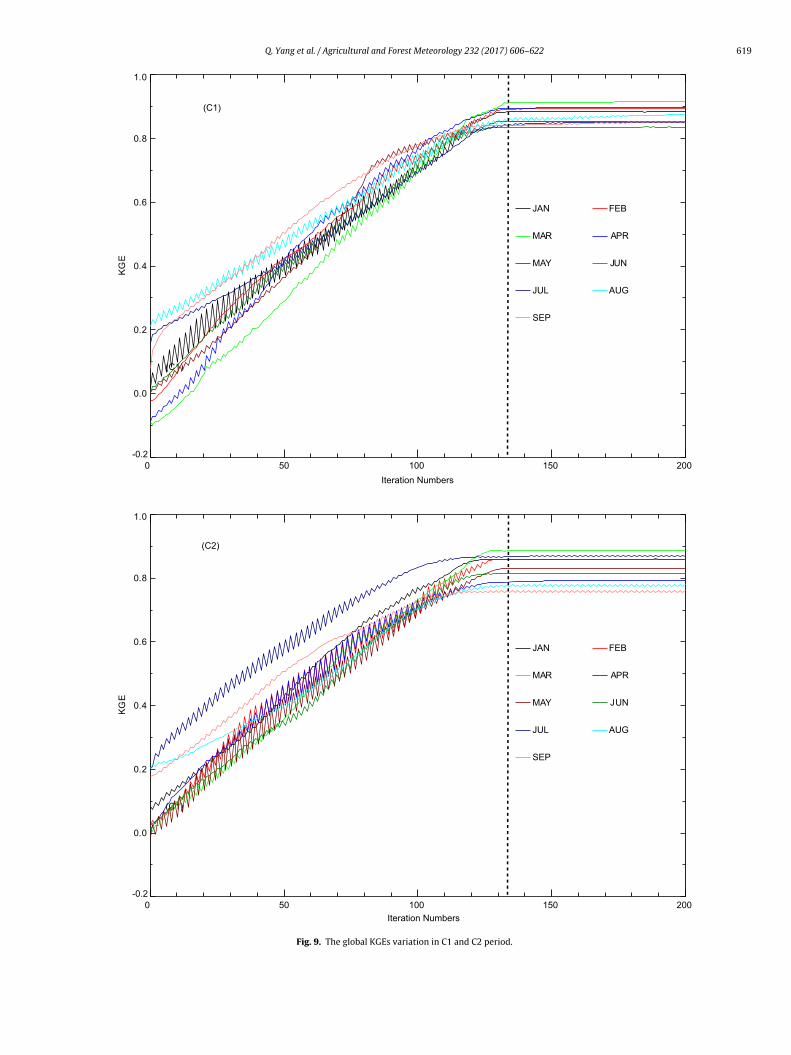
Figs. 6 and 7 show a comparison of the calculated and mea-sured momentum fluxes. Fig. 8 shows the diurnal variations ofmomentum flux MBE in C1 and V1 period. Table 4 shows numerousstatistics for the calculated momentum flux. The pattern resem-bled that of the sensible heat flux. Furthermore, the global KGEsvariation in C1 and C2 period was represented in Fig. 9 to betterunderstand the calibration process. As show in Fig. 9, the globalKGEs were converged after about 130 iterative times in everymonth, with all the values greater than 0.75.It implied that cali-bration process generated by the PSO algorithm and the MOST wasrather stable and efficient.

In summary, the combination of the MOST and the PSO algo-rithm was able to simultaneously calibrate the turbulent fluxparameters. The calibrated parameters enabled the fluxes of sen-sible heat and momentum fluxes to be reliably determined fordifferent time periods. The calibration process was stable and effi-cient. In addition, this calibration process was neither limited toneutral conditions nor dependent on the profiles of the multi-layerwind velocity and potential temperature being very accurate as theconventional approach.

The variations of the calibrated parameters were depicted inFig. 10. Table 5 lists the calibrated parameters during the C1 andC2 periods. As shown in Fig. 10, there were monthly variationsin the calibrated parameters during the same calibration period.In addition, the calibrated parameters for a given month differedin the two periods. The empirical parameters did not exhibit anymonthly trend, indicating a wide range of variations on a monthlyscale. Therefore, the present similarity functions were not appli-

cable to every month. Furthermore, the calculated annual meanvalues of ˇm, ˇh, �m and �h were 17.4, 14.1, 4.6 and 5.5 and 17.8,15.6, 4.5 and 4.7 during the C1 and C2 periods, respectively. Onan annual scale, the variations in these parameters were relatively

612 Q. Yang et al. / Agricultural and Forest Meteorology 232 (2017) 606–622

Measured Calibrated ValidatedJAN

1-01 1-05 1-10 1-15 1-20 1-25 1-30-100

0

100

200

300

400

500

SE

N (W

m

)-2

Measured Calibrated ValidatedFEB

2-01 2-05 2-10 2-15 2-20 2-25 2-28-100

0

100

200

300

400

500S

EN

(W m

)

-2

Measured Calibrated ValidatedMAR

3-01 3-05 3-10 3-15 3-20 3-25 3-30-100

0

100

200

300

400

500

SE

N (W

m

)-2

Measured Calibrated ValidatedAPR

4-01 4-05 4-10 4-15 4-20 4-25 4-30-100

0

100

200

300

400

500

SE

N (W

m

)-2

Measured Calibrated ValidatedMAY

5-01 5-05 5-10 5-15 5-20 5-25 5-30-100

0

100

200

300

400

500

SE

N (W

m

)-2

Measured Calibrated ValidatedJUN

6-01 6-05 6-10 6-15 6-20 6-25 6-30-100

0

100

200

300

400

500

SE

N (W

m

)-2

Measured Calibrated ValidatedJUL

7-01 7-05 7-10 7-15 7-20 7-25 7-30-100

0

100

200

300

400

500

SE

N (W

m

)-2

Measured Calibrated ValidatedAUG

8-01 8-05 8-10 8-15 8-20 8-25 8-30-100

0

100

200

300

400

500

SE

N (W

m

)-2

Measured Calibrated ValidatedSEP

9-01 9-05 9-10 9-15 9-20 9-25 9-30-100

0

100

200

300

400

500

SE

N (W

m

)-2

Fig. 3. Comparison of the calculated sensible (SEN) heat flux against measurement.

Q. Yang et al. / Agricultural and Forest Meteorology 232 (2017) 606–622 613

Table 2The ranges of the parameters to be calibrated.

Variable Symbol Range

Momentum empirical parameters for stable ˇm [2,8]Sensible heat empirical parameters for stable ˇh [2,8]Momentum empirical parameters for unstable �m [10,30]Sensible heat empirical parameters for unstable �h [10,30]Aeroaerodynamic roughness z0m [1e-4,1.0]Parameter related with thermal and aeroaerodynamic roughness Kb−1 [0,20]

(C1) JAN

-100 0 100 200 300 400Measured SEN (Wm )

-100

0

100

200

300

400

Cac

ulat

ed S

EN

(Wm

)

N= 594

KGE= 0.88

y =1.06x-4.06

R = 0.95

-2

-2

(V1) JAN

-100 0 100 200 300 400Measured SEN (Wm )

-100

0

100

200

300

400C

acul

ated

SE

N (W

m

)

N= 560

KGE= 0.72

y =1.24x-4.35

R = 0.95

-2

-2

(C1) FEB

-100 0 100 200 300 400Measured SEN (Wm )

-100

0

100

200

300

400

Cac

ulat

ed S

EN

/(Wm

)

N= 658

KGE= 0.88

y =1.09x-4.58

R = 0.97

-2

-2

(V1) FEB

-100 0 100 200 300 400Measured SEN (Wm )

-100

0

100

200

300

400

Cac

ulat

ed S

EN

(Wm

)

N= 658

KGE= 0.70

y =1.26x-4.35

R = 0.96

-2

-2

(C1) MA R

-100 0 100 200 300 400Measured SEN (Wm )

-100

0

100

200

300

400

Cac

ulat

ed S

EN

(Wm

)

N= 792

KGE= 0.90

y =1.08x-5.34

R = 0.98

-2

-2

(V1) MAR

-100 0 100 200 300 400Measured SEN (Wm )

-100

0

100

200

300

400

Cac

ulat

ed S

EN

(Wm

)

N= 788

KGE= 0.85

y =1.14x-4.85

R = 0.97

-2

-2

(C1) APR

-100 0 100 200 300 400Measured SEN (Wm )

-100

0

100

200

300

400

Cac

ulat

ed S

EN

(Wm

)

N= 769

KGE= 0.89

y =1.09x-7.71

R = 0.97

-2

-2

(V1) APR

-100 0 100 200 300 400Measured SEN (Wm )

-100

0

100

200

300

400

Cac

ulat

ed S

EN

(Wm

)

N= 722

KGE= 0.72

y =1.28x-9.28

R = 0.97

-2

-2

(C1) MA Y

-100 0 100 200 300 400-100

0

100

200

300

400

Cac

ulat

ed S

EN

(Wm

)

N= 436

KGE= 0.92

y =1.05x-1.53

R = 0.97

-2

-2

(V1) MAY

-100 0 100 200 300 400Measured SEN (Wm )

-100

0

100

200

300

400

Cac

ulat

ed S

EN

(Wm

)

N= 433

KGE= 0.82

y =1.15x-1.94

R = 0.97

-2

-2

(V1) JUN

-100 0 100 200 300 400Measured SEN (Wm )

-100

0

100

200

300

400

Cac

ulat

ed S

EN

(Wm

)

N= 922

KGE= 0.83

y =1.08x-0.01

R = 0.94

-2

-2

(C1) JUN

-100 0 100 200 300 400Measured SEN (Wm )

-100

0

100

200

300

400

Cac

ulat

ed S

EN

(Wm

)

N= 927

KGE= 0.92

y =0.97x-0.25

R = 0.94

-2

-2

(C1) JUL

-100 0 100 200 300 400Measured SEN (Wm )

-100

0

100

200

300

400

Cac

ulat

ed S

EN

(Wm

)

N= 1044

KGE= 0.89

y =0.96x+0.26

R = 0.91

-2

-2

(V1) JUL

-100 0 100 200 300 400Measured SEN (Wm )

-100

0

100

200

300

400

Cac

ulat

ed S

EN

(Wm

)

N= 1039

KGE= 0.86

y =1.02x-1.48

R = 0.91

-2

-2

-2

(C1) AUG

-100 0 100 200 300 400Measured SEN (Wm )

-100

0

100

200

300

400

Cac

ulat

ed S

EN

(Wm

)

N= 554

KGE= 0.95

y =0.98x+1.35

R = 0.96

-2

-2

(V1) AUG

-100 0 100 200 300 400Measured SEN (Wm )

-100

0

100

200

300

400

Cac

ulat

ed S

EN

(Wm

) N= 546

KGE= 0.84

y =1.09x+0.75

R = 0.97

-2

-2

(C1) SEP

-100 0 100 200 300 400Measured SEN (Wm )

-100

0

100

200

300

400

Cac

ulat

ed S

EN

(Wm

)

N= 763

KGE= 0.95

y =0.99x+0.99

R = 0.96

-2

-2

(V1) SEP

-100 0 100 200 300 400Measured SEN (Wm )

-100

0

100

200

300

400

Cac

ulat

ed S

EN

(Wm

)

N= 765

KGE= 0.95

y =0.95x+0.58

R = 0.97

-2

-2

Fig. 4. Scatter plot of the sensible (SEN) heat flux calculation against measurement.

614 Q. Yang et al. / Agricultural and Forest Meteorology 232 (2017) 606–622

(C1)

0 4 8 12 16 20 24-50

-30

-10

10

30

50

SE

N M

BE

(W m

)

JAN FEB

MAR APR

MAY JUN

JUL AUG

SEP

-2

HOUR

(V1)

0 4 8 12 16 20 24-50

-30

-10

10

30

50

SE

N B

ias

(W m

)

JAN FEB

MAR APR

MAY JUN

JUL AUG

SEP

-2

HOUR

Fig. 5. The diurnal variations of sensible (SEN) heat flux MBE in C1 and V1 period.

Q. Yang et al. / Agricultural and Forest Meteorology 232 (2017) 606–622 615

Measured Calibrated ValidatedJAN

1-01 1-05 1-10 1-15 1-20 1-25 1-300.0

0.2

0.4

0.6

0.8

1.0

1.2

MO

M (k

g m

s

)-2

-1Measured Calibrated ValidatedFEB

2-01 2-05 2-10 2-15 2-20 2-25 2-280.0

0.2

0.4

0.6

0.8

1.0

1.2

MO

M (k

g m

s

)-2

-1

Measured Calibrated ValidatedMAR

3-01 3-05 3-10 3-15 3-20 3-25 3-300.0

0.2

0.4

0.6

0.8

1.0

1.2

MO

M (k

g m

s

)-2

-1

Measured Calibrated ValidatedAPR

4-01 4-05 4-10 4-15 4-20 4-25 4-300.0

0.2

0.4

0.6

0.8

1.0

1.2

MO

M (k

g m

s

)-2

-1

Measured Calibrated ValidatedMAY

5-01 5-05 5-10 5-15 5-20 5-25 5-300.0

0.2

0.4

0.6

0.8

1.0

1.2

MO

M (k

g m

s

)-2

-1

Measured Calibrated ValidatedJUN

6-01 6-05 6-10 6-15 6-20 6-25 6-300.0

0.2

0.4

0.6

0.8

1.0

1.2

MO

M (k

g m

s

)-2

-1

Measured Calibrated ValidatedJUL

7-01 7-05 7-10 7-15 7-20 7-25 7-300.0

0.2

0.4

0.6

0.8

1.0

1.2

MO

M (k

g m

s

) -2

-1

Measured Calibrated ValidatedAUG

8-01 8-05 8-10 8-15 8-20 8-25 8-300.0

0.2

0.4

0.6

0.8

1.0

1.2

MO

M (k

g m

s

)-2

-1

Measured Calibrated ValidatedSEP

9-01 9-05 9-10 9-15 9-20 9-25 9-300.0

0.2

0.4

0.6

0.8

1.0

1.2

MO

M (k

g m

s

)-2-1

Fig. 6. Comparison of the calculated momentum (MOM) flux against measurement.

616 Q. Yang et al. / Agricultural and Forest Meteorology 232 (2017) 606–622

Table 3Mean Values of the observed (Mean Obs) and calculated (Mean Cal) sensible heat flux; the Intercept, Slope, and R of the Linear Fit coefficients; and the RMSE, MBE and KGEvalue for different calibration and validation period (in brackets).

Mean Obs Mean Cal Slope Intercept R MBE RMSE KGE

JAN(C1/V1) 68.45 68.56 (73.46) 1.06 (1.24) −4.06 (−4.35) 0.95 (0.95) 0.12 (10.82) 23.69 (34.34) 0.88 (0.72)JAN(C2/V2) 39.11 36.04 (28.82) 1.05 (0.84) −5.02 (−3.92) 0.92 (0.93) −3.07 (−10.29) 27.88 (25.26) 0.83 (0.72)FEB(C1/V1) 45.86 45.37 (60.50) 1.09 (1.26) −4.58 (−4.35) 0.97 (0.96) −0.49 (10.67) 19.82 (31.62) 0.88 (0.70)FEB(C2/V2) 59.07 54.64 (43.86) 1.06 (0.91) −8.12 (−9.69) 0.95 (0.95) −4.42 (−15.21) 29.87 (28.71) 0.85 (0.65)MAR(C1/V1) 57.67 56.72 (61.69) 1.08 (1.14) −5.34 (−4.85) 0.98 (0.97) −0.95 (3.19) 21.74 (25.52) 0.90 (0.85)MAR(C2/V1) 65.03 60.70 (53.91) 1.04 (0.93) −7.26 (−6.19) 0.95 (0.95) −4.33 (−10.65) 32.01 (29.28) 0.87 (0.80)APR(C1/V1) 68.56 66.94 (76.43) 1.09 (1.28) −7.71 (−9.28) 0.97 (0.97) −1.62 (9.66) 24.68 (39.09) 0.89 (0.72)APR(C2/V2) 56.18 52.07 (59.17) 1.01 (1.18) −4.72 (−7.17) 0.96 (0.96) −4.11 (2.98) 23.22 (30.00) 0.90 (0.80)MAY(C1/V1) 34.36 34.51 (35.52) 1.05 (1.15) −1.53 (−1.94) 0.97 (0.97) −0.15 (2.97) 14.79 (18.09) 0.92 (0.82)MAY(C2/V2) 44.91 42.53 (42.02) 1.07 (1.05) −5.44 (−4.95) 0.95 (0.95) −2.38 (−2.89) 24.63 (24.11) 0.86 (0.86)JUN(C1/V1) 29.15 28.18 (31.10) 0.97 (1.08) −0.25 (−0.01) 0.94 (0.94) −0.97 (2.39) 14.53 (16.47) 0.92 (0.83)JUN(C2/V2) 34.39 33.28 (34.38) 0.98 (1.02) −0.47 (−0.56) 0.95 (0.94) −1.10 (−0.07) 16.21 (17.09) 0.93 (0.91)JUL(C1/V1) 27.36 26.51 (25.40) 0.96 (1.02) 0.26 (−1.48) 0.91 (0.91) −0.85 (−0.97) 17.07 (17.55) 0.89 (0.86)JUL(C2/V2) 21.41 21.35 (20.82) 0.96 (0.94) 0.79 (0.68) 0.95 (0.95) −0.06 (−0.59) 12.18 (12.37) 0.95 (0.94)AUG(C1/V1) 31.58 32.37 (34.83) 0.98 (1.09) 1.35 (0.75) 0.96 (0.97) 0.79 (3.56) 12.52 (14.20) 0.95 (0.84)AUG(C2/V2) 36.13 34.08 (29.87) 0.98 (0.86) −1.19 (−1.26) 0.91 (0.90) −2.05 (−6.26) 22.04 (21.81) 0.87 (0.76)SEP(C1/V1) 36.74 37.33 (34.94) 0.99 (0.95) 0.99 (0.58) 0.96 (0.97) 0.59 (−1.21) 13.36 (12.47) 0.95 (0.95)SEP(C2/V2) 43.18 40.27 (57.70) 1.00 (1.21) −2.89 (−3.51) 0.90 (0.90) −2.89 (4.52) 27.62 (29.39) 0.84 (0.75)

Table 4Mean Values of the measurement and calculated momentum flux; the Intercept, Slope, and R of the Linear Fit coefficients; and the RMSE, MBE and KGE value for differentcalibration and validation period (in brackets).

Mean Obs Mean Cal Slope Intercept R MBE RMSE KGE

JAN(C1/V1) 0.084 0.086 (0.101) 1.03(1.32) −0.001(0.001) 0.95(0.95) 0.002 (0.025) 0.034 (0.055) 0.89 (0.62)JAN(C2/V2) 0.064 0.062(0.042) 0.94(0.71) 0.002(−0.003) 0.91(0.93) −0.002 (−0.008) 0.038(0.042) 0.90(0.71)FEB(C1/V1) 0.061 0.060 (0.072) 0.95(1.07) 0.002(0.001) 0.92(0.89) −0.001 (0.005) 0.026(0.036) 0.91 (0.79)FEB(C2/V2) 0.081 0.075(0.063) 1.03(0.87) −0.008(−0.006) 0.93(0.95) −0.006(−0.017) 0.041(0.037) 0.87(0.71)MAR(C1/V1) 0.092 0.091 (0.097) 1.00(1.08) −0.001(−0.004) 0.95(0.96) −0.001 (0.004) 0.030(0.036) 0.94(0.87)MAR(C2/V1) 0.106 0.101(0.085) 0.98(0.86) −0.002(−0.005) 0.93(0.93) −0.005(−0.019) 0.048(0.049) 0.90(0.75)APR(C1/V1) 0.094 0.095 (0.117) 1.04(1.32) −0.003(−0.004) 0.95(0.95) 0.001 (0.025) 0.030(0.054) 0.90(0.64)APR(C2/V2) 0.078 0.071(0.054) 0.88(0.78) 0.010(0.005) 0.81(0.81) −0.007(−0.024) 0.051(0.056) 0.78(0.63)MAY(C1/V1) 0.073 0.075 (0.085) 1.06(1.19) −0.001(0.001) 0.87(0.88) 0.002 (0.014) 0.036 (0.042) 0.78 (0.67)MAY(C2/V2) 0.084 0.079(0.071) 0.84(0.83) 0.019(0.018) 0.79(0.79) −0.006(−0.003) 0.064(0.063) 0.79(0.73)JUN(C1/V1) 0.054 0.065 (0.064) 0.84(0.82) 0.019(0.019) 0.81(0.81) 0.011 (0.009) 0.036 (0.035) 0.75 (0.73)JUN(C2/V2) 0.067 0.067(0.075) 0.80(0.86) 0.019(0.024) 0.81(0.79) −0.006(0.007) 0.049(0.054) 0.71(0.66)JUL(C1/V1) 0.054 0.055(0.079) 0.94(1.25) 0.004(0.009) 0.85(0.85) 0.001 (0.008) 0.024 (0.026) 0.83 (0.77)JUL(C2/V2) 0.081 0.089(0.067) 0.85(0.81) 0.005(0.004) 0.82(0.85) 0.008(−0.013) 0.066(0.062) 0.79(0.70)AUG(C1/V1) 0.058 0.063 (0.074) 1.11(1.14) −0.002(−0.003) 0.92(0.92) −0.005 (0.016) 0.027 (0.041) 0.80 (0.70)AUG(C2/V2) 0.047 0.045(0.036) 0.83(0.81) 0.011(0.007) 0.83(0.81) −0.002(−0.011) 0.041(0.039) 0.70(0.74)SEP(C1/V1) 0.049 0.062 (0.064) 1.11(1.21) 0.004(0.011) 0.84(0.83) 0.014 (0.016) 0.040 (0.038) 0.78 (0.71)SEP(C2/V2) 0.059 0.058(0.069) 0.81(0.80) 0.016(0.021) 0.90(0.89) −0.001(0.009) 0.048(0.054) 0.70(0.63)

Table 5Values of Calibrated parameters relating to the monthly turbulent flux.

ˇm, ˇh �m �h z0m (cm) Kb−1

JAN(C1) 17.49 14.56 6.58 5.62 0.93 5.41JAN(C2) 20.05 17.80 6.02 3.71 1.84 6.66FEB(C1) 16.16 11.09 3.37 3.89 0.73 6.87FEB(C2) 21.19 19.83 6.31 6.32 1.13 6.60MAR(C1) 17.09 12.89 3.74 6.36 0.59 7.48MAR(C2) 18.59 12.90 3.65 4.71 0.86 6.30APR(C1) 13.07 10.09 4.21 6.23 0.61 6.50APR(C2) 10.58 10.21 2.50 4.77 1.41 7.46MAY(C1) 16.18 15.41 3.04 5.66 0.77 6.96MAY(C2) 11.17 10.96 3.14 3.50 1.41 7.49JUN(C1) 17.80 17.33 5.69 5.96 1.22 6.12JUN(C2) 19.28 19.14 4.90 5.79 1.31 6.37JUL(C1) 15.40 12.86 4.06 5.53 2.82 1.81JUL(C2) 16.98 15.84 2.59 4.19 3.10 4.34AUG(C1) 23.93 19.53 5.27 4.81 2.04 1.44

5.535.745.43

stiKu

AUG(C2) 21.21 18.90

SEP(C1) 19.40 13.28

SEP(C2) 20.99 14.93

mall. The characteristic variations in z0m were consistent during

he C1 and C2 periods, with a minimum in March and a maximumn August (C1) or September (C2). The characteristic variations inb−1 were also consistent in periods C1 and C2, with higher val-es between January and June and lower values between July and

5.28 3.89 2.10 5.31 3.16 2.22 4.14 2.66 3.76

September. But as shown in Table 5, the values of z0m and Kb−1 were

different in C1 and C2 periods, which implied that the differencewould affect the validation process and result in the deviations. Todecrease the deviation, several years’ data should be employed to

Q. Yang et al. / Agricultural and Forest Meteorology 232 (2017) 606–622 617

(C1) JAN

0.0 0.2 0.4 0.6 0.8 1.0Measured MOM (kg m s )

0.0

0.2

0.4

0.6

0.8

1.0C

alcu

late

d M

OM

(kg

m s

)

N= 594

KGE= 0.89

y =1.03x-0.001

R = 0.95

-2-1

-2-1

(V1) JAN

0.0 0.2 0.4 0.6 0.8 1.0Measured MOM (kg m s )

0.0

0.2

0.4

0.6

0.8

1.0

Cal

cula

ted

MO

M (k

g m

s

)

N= 560

KGE= 0.62

y =1.32x-0.001

R = 0.95

-2 -1

-2-1

(C1) FEB

0.0 0.2 0.4 0. 6 0. 8 1. 0Measured MOM (kg m s )

0.0

0.2

0.4

0.6

0.8

1.0

Cal

cula

ted

MO

M (k

g m

s

)

N= 658

KGE= 0.91

y =0.95x+0.002

R = 0.92

-2 -1

-2 -1

(V1) FEB

0.0 0.2 0.4 0. 6 0. 8 1. 0Measured MOM (kg m s )

0.0

0.2

0.4

0.6

0.8

1.0

Cal

cula

ted

MO

M (k

g m

s

)

N= 658

KGE= 0.79

y =1.07x+0.001

R = 0.89

-2-1

-2-1

(C1) MAR

0.0 0.2 0.4 0. 6 0. 8 1. 0Measured MOM (kg m s )

0.0

0.2

0.4

0.6

0.8

1.0

Cal

cula

ted

MO

M (k

g m

s

)

N= 792

KGE= 0.94

y =1.00x-0.001

R = 0.95

-2 -1

-2-1

(V1) MA R

0.0 0.2 0.4 0. 6 0. 8 1. 0Measured MOM (kg m s )

0.0

0.2

0.4

0.6

0.8

1.0

Cal

cula

ted

MO

M (k

g m

s

)

N= 788

KGE= 0.87

y =1.08x-0.004

R = 0.96

-2-1

-2-1

(C1) APR

0.0 0.2 0.4 0. 6 0. 8 1. 0Measured MOM (kg m s )

0.0

0.2

0.4

0.6

0.8

1.0

Cal

cula

ted

MO

M (k

g m

s

)

N= 769

KGE= 0.90

y =1.04x-0.003

R = 0.95

-2 -1

-2 -1

(V1) APR

0.0 0.2 0.4 0. 6 0. 8 1. 0Measured MOM (kg m s )

0.0

0.2

0.4

0.6

0.8

1.0

Cal

cula

ted

MO

M (k

g m

s

)

N= 722

KGE= 0.64

y =1.32x-0.004

R = 0.95

-2-1

-2-1

(C1) MAY

0.0 0.2 0.4 0. 6 0. 8 1. 0Measured MOM (kg m s )

0.0

0.2

0.4

0.6

0.8

1.0

Cal

cula

ted

MO

M (k

g m

s

)

N= 436

KGE= 0.78

y =1.06x-0.001

R = 0.87

-2 -1

-2-1

(V1) MA Y

0.0 0.2 0.4 0. 6 0. 8 1. 0Measured MOM (kg m s )

0.0

0.2

0.4

0.6

0.8

1.0

Cal

cula

ted

MO

M (k

g m

s

)

N= 433

KGE= 0.67

y =1.19x+0.001

R = 0.88

-2-1

-2-1

(C1) JUN

0.0 0.2 0.4 0.6 0.8 1.0Measured MOM (kg m s )

0.0

0.2

0.4

0.6

0.8

1.0

Cal

cula

ted

MO

M (k

g m

s

)

N= 927

KGE= 0.75

y =0.84x+0.019

R = 0.81

-2 -1

-2-1

(V1) JU N

0.0 0.2 0.4 0.6 0.8 1.0Measured MOM (kg m s )

0.0

0.2

0.4

0.6

0.8

1.0

Cal

cula

ted

MO

M (k

g m

s

)

N= 922

KGE= 0.73

y =0.82x+0.019

R = 0.81

-2-1

-2-1

(C1) JUL

0.0 0.2 0.4 0. 6 0. 8 1. 0Measured MOM (kg m s )

0.0

0.2

0.4

0.6

0.8

1.0

Cal

cula

ted

MO

M (k

g m

s

)

N= 1044

KGE= 0.83

y =0.94x+0.004

R = 0.85

-2 -1

-2 -1

(V1) JU L

0.0 0.2 0.4 0. 6 0. 8 1. 0Measured MOM (kg m s )

0.0

0.2

0.4

0.6

0.8

1.0

Cal

cula

ted

MO

M (k

g m

s

)

N= 1039

KGE= 0.77

y =1.25x+0.009

R = 0.85

-2 -1

-2-1

(C1) AUG

0.0 0.2 0.4 0. 6 0. 8 1. 0Measured MOM (kg m s )

0.0

0.2

0.4

0.6

0.8

1.0

Cal

cula

ted

MO

M (k

g m

s

)

N= 554

KGE= 0.80

y =1.11x-0.002

R = 0.92

-1 -2

-2-1

(V1) AU G

0.0 0.2 0.4 0. 6 0. 8 1. 0Measured MOM (kg m s )

0.0

0.2

0.4

0.6

0.8

1.0

Cal

cula

ted

MO

M (k

g m

s

)

N= 546

KGE= 0.70

y =1.14x-0.003

R = 0.92

-2-1

-2-1

(C1) SEP

0.0 0.2 0.4 0. 6 0. 8 1. 0Measured MOM (kg m s )

0.0

0.2

0.4

0.6

0.8

1.0

Cal

cula

ted

MO

M (k

g m

s

)

N= 763

KGE= 0.78

y =1.11x+0.004

R = 0.84

-2 -1

-2-1

(V1) SEP

0.0 0.2 0.4 0. 6 0. 8 1. 0Measured MOM (kg m s )

0.0

0.2

0.4

0.6

0.8

1.0

Cal

cula

ted

MO

M (k

g m

s

)

N= 765

KGE= 0.71

y =1.21x+0.011

R = 0.83

-2 -1

-2-1

OM)

cn

5

fu

Fig. 7. Scatter plot of the momentum (M

alibrate parameters and the mean value may be more suitable forumerical modeling.

. Conclusions and discussions

Land-atmosphere exchanges of mass and energy determine theundamental characteristics of a regional climate. Therefore, tonderstand regional climates and hydrological cycles, it is impor-

flux calculation against measurement.

tant to determine the parameters that relate to the turbulent fluxin the surface layer and to develop optimal turbulent flux parame-terization schemes using near-surface synthesis measurements. Innumerical modeling, the turbulent flux parameterization is gen-

erally based on MOST. According to this theory, it is necessaryto simultaneously determine the empirical similarity parametersˇm, ˇh, �m and �h, the aerodynamic roughness (z0m) and the ther-mal roughness (zT ). However, it is difficult to determine these six

618 Q. Yang et al. / Agricultural and Forest Meteorology 232 (2017) 606–622

0 4 8 12 16 20 24-0.10

-0.06

-0.02

0.02

0.06

0.10

MO

M M

BE

(kg

m

s )

(C1) JAN FEB MAR APR MAY

JUN JUL AUG SEP

-2

-1

HOUR

(V1)

0 4 8 12 16 20 24-0.10

-0.06

-0.02

0.02

0.06

0.10

MO

M M

BE

(kg

m

s

)

JAN FEB MAR APR MAY

JUN JUL AUG SEP

-2

-1

HOUR

Fig. 8. The diurnal variations of momentum (MOM) flux MBE in C1 and V1 period.

Q. Yang et al. / Agricultural and Forest Meteorology 232 (2017) 606–622 619

JAN FEB

MAR APR

MAY JUN

JUL AUG

SEP

(C1)

0 50 100 150 200-0.2

0.0

0.2

0.4

0.6

0.8

1.0

KG

E(C1)

Iteration Numbers

JAN FEB

MAR APR

MAY JUN

JUL AUG

SEP

(C1)

0 50 100 150 200-0.2

0.0

0.2

0.4

0.6

0.8

1.0

KG

E

Iteration Numbers

(C2)

Fig. 9. The global KGEs variation in C1 and C2 period.

620 Q. Yang et al. / Agricultural and Forest Meteorology 232 (2017) 606–622

C1 C2(a)

JAN FEB MA R AP R MAY JU N JU L AU G SEP0

5

10

15

20

25

30

βm

C1 C2(b)

JAN FEB MA R AP R MAY JU N JU L AU G SEP0

5

10

15

20

25

30

βh

C1 C2(c)

JAN FEB MA R AP R MAY JU N JU L AU G SEP0

2

4

6

8

10

γm

C1 C2(d)

JAN FEB MA R AP R MAY JU N JU L AU G SEP0

2

4

6

8

10

γh

C1 C2(e)

JAN FEB MA R AP R MAY JU N JU L AU G SEP0

1

2

3

4

5

Z0m (m

)

C1 C2(f)

JAN FEB MA R AP R MAY JU N JU L AU G SEP0

2

4

6

8

10

Kb-1

Fig. 10. The variations of the calibrated parameters during the C1 and C2 periods.

rest M

pTsbrtp

(

(

bTosastTbtamsfPpstwbiotbfl

A

Wt(Con

R

A

B

Q. Yang et al. / Agricultural and Fo

arameters simultaneously by solving a set of nonlinear equations.he artificial intelligence algorithm provides a feasible approach toolving this problem. With measurements from Maqu Station as aasis, this study used the PSO algorithm to calibrate the parameterselating to the monthly turbulent flux at the surface and calculatedhe fluxes of sensible heat and momentum using the calibratedarameters. This study concluded the following:

1) Using the PSO algorithm, the surface layer turbulent fluxparameters can be calibrated simultaneously. The fluxes ofsensible heat and momentum calculated with the calibratedparameters using MOST were close and highly correlated to themeasured values; their linear fit lines had slopes of nearly one.

2) The calibrated empirical similarity parameters showedmonthly variations that did not have any trend, which sug-gested that there is a wide range of monthly variation in theseempirical parameters, and the present similarity functionsmay not be fully applicable to every month. The characteristicvariations in z0m and Kb−1 were consistent while the valueswere different in two calibration periods. Therefore, deviationsmay be introduced when these parameters transferred outsidethe calibration periods.

Our study showed that the PSO algorithm can be used to cali-rate the parameters relating to turbulent flux in the surface layer.here still exist a few problems in using the PSO algorithm orther optimization algorithms, which must be addressed in futuretudies, as follows: (1) Parameters obtained by an optimizationlgorithm should be further tested against observations. In fact, theurface layer parameters or parameter combinations calibrated byhe PSO algorithm are only optimal solutions of MOST equations.hese solutions have no specific physical meanings. How to com-ine the optimal solution with the actual physical process requiredo further proved; (2) As a major drawback of the PSO algorithm,

number of parameters inherent to algorithm have to be deter-ined, though these parameters have no effect on the optimal

olution. Like other optimization algorithms, if a multi-objectiveunction is defined in the PSO algorithm, we can only obtain theareto solution of the problem; (3) The number of calibrationarameters should be limited. Because each parameter can beelected within its range. With the number of calibration parame-ers increased, the corresponding combinations for the parametersere also increased. However, Finding the optimal solution would

e more difficult within finite times and iterations. In summary,t is of equal importance to conduct comprehensive near-surfacebservational experiments, and combine optimization algorithmso accurately identify surface layer parameters or parameter com-inations, which can eventually improve the accuracy of turbulentuxes between atmosphere and land surface.

cknowledgments

This work is supported by the R&D Special Fund for Publicelfare Industry (GYHY201406001), Natural Science Founda-

ion of China (41305103 and 41275162) and Yunnan Province2013FD005), and the Jiangsu Collaborative Innovation Center forlimate Change. We also thank the Maqu station for providing thebservation data and High Performance Computing Center of Yun-an University for computational support.

eferences

bdella, K., McFarlane, N.A., 1996. Parameterization of the surface-layer exchangecoefficients for atmospheric models. Boundary-Layer Meteorol. 80 (3),223–248.

eljaars, A.C.M., Holtslag, A.A.M., 1991. Flux parameterization over land surfacesfor atmospheric models. J. Appl. Meteorol. 30 (3), 327–341.

eteorology 232 (2017) 606–622 621

Businger, J.A., Wyngaard, J.C., Izumi, Y., Bradley, E.F., 1971. Flux-profilerelationships in the atmospheric surface layer. J. Atmos. Sci. 28 (2),181–189.

Chau, K.W., 2006. Particle swarm optimization training algorithm for ANNs instage prediction of Shing Mun River. J. Hydrol. 329 (3–4), 363–367.

Chen, F., Janjic, Z., Mitchell, K., 1997. Impact of atmospheric surface-layerparameterizations in the new land-surface scheme of the NCEP mesoscale etamodel. Boundary-Layer Meteorol. 85 (3), 391–421.

Crow, W.T., Wood, E.F., Pan, M., 2003. Multiobjective calibration of land surfacemodel evapotranspiration predictions using streamflow observations andspaceborne surface radiometric temperature retrievals. J. Geophys. Res.:Atmos. 108 (D23), 4725.

Cuo, L., Zhang, Y., Gao, Y., Hao, Z., Cairang, L., 2013. The impacts of climate changeand land cover/use transition on the hydrology in the upper Yellow RiverBasin, China. J. Hydrol. 502, 37–52.

Dai, Y., et al., 2003. The common land model. Bull. Am. Meteorol. Soc. 84 (8),1013–1023.

Dickinson, R.E., Shaikh, M., Bryant, R., Graumlich, L., 1998. Interactive canopies fora climate model. J. Clim. 11 (11), 2823–2836.

Dyer, A.J., 1974. A review of flux-profile relationships. Boundary-Layer Meteorol. 7(3), 363–372.

Fu, G., Chen, S., Liu, C., Shepard, D., 2004. Hydro-climatic trends of the yellow riverbasin for the last 50 years. Clim. Change 65 (1), 149–178.

Garratt, J.R., Pielke, R.A., 1989. On the sensitivity of mesoscale models tosurface-layer parameterization constants. Boundary-Layer Meteorol. 48 (4),377–387.

Gill, M.K., Kaheil, Y.H., Khalil, A., McKee, M., Bastidas, L., 2006. Multiobjectiveparticle swarm optimization for parameter estimation in hydrology. WaterResour. Res. 42 (7), 257–271.

Gupta, H.V., Bastidas, L.A., Sorooshian, S., Shuttleworth, W.J., Yang, Z.L., 1999.Parameter estimation of a land surface scheme using multicriteria methods. J.Geophys. Res.: Atmos. 104 (D16), 19491–19503.

Gupta, H.V., Kling, H., Yilmaz, K.K., Martinez, G.F., 2009. Decomposition of themean squared error and NSE performance criteria: implications for improvinghydrological modelling. J. Hydrol. 377 (1–2), 80–91.

Högström, U., 1988. Non-dimensional wind and temperature profiles in theatmospheric surface layer: a re-evaluation. Boundary-Layer Meteorol. 42 (1),55–78.

Högström, U., 1996. Review of some basic characteristics of the atmosphericsurface layer. Boundary-Layer Meteorol. 78 (3), 215–246.

Hu, Y., Maskey, S., Uhlenbrook, S., 2012. Trends in temperature and rainfallextremes in the Yellow River source region, China. Clim. Change 110 (1),403–429.

Kanda, M., Kanega, M., Kawai, T., Moriwaki, R., Sugawara, H., 2007. Roughnesslengths for momentum and heat derived from outdoor urban scale models. J.Appl. Meteorol. Climatol. 46 (7), 1067–1079.

Kennedy, J., Eberhart, R., 1995. Particle swarm optimization. Proc. IEEE Int. Conf.Neural Networks 4, 1942–1948.

Łobocki, L., 1993. A procedure for the derivation of surface-layer bulk relationshipsfrom simplified second-order closure models. J. Appl. Meteorol. 32 (1),126–138.

Louis, J.-F., 1979. A parametric model of vertical eddy fluxes in the atmosphere.Boundary-Layer Meteorol. 17 (2), 187–202.

MacKinnon, D.J., Clow, G.D., Tigges, R.K., Reynolds, R.L., Chavez Jr., P.S., 2004.Comparison of aerodynamically and model-derived roughness lengths (zo)over diverse surfaces, central Mojave Desert, California, USA. Geomorphology63 (1–2), 103–113.

Monin, A.S., Obukhov, A.M., 1954. Basic laws of turbulent mixing in the surfacelayerof the atmosphere. Tr. Akad. Nauk SSSR Geophiz. Inst. 24 (151),163–187.

Niu, G.-Y., et al., 2011. The community Noah land surface model withmultiparameterization options (Noah-MP): 1. Model description andevaluation with local-scale measurements. J. Geophys. Res.: Atmos. 116 (D12),1248–1256.

Oleson, K.W. et al. 2010. Technical Description of version 4.0 of the CommunityLand Model (CLM). NCAR Technical Note NCAR/TN-478+STR.

Paulson, C.A., 1970. The mathematical representation of wind speed andtemperature profiles in the unstable atmospheric surface layer. J. Appl.Meteorol. 9 (6), 857–861.

Poli, R., Kennedy, J., Blackwell, T., 2007. Particle swarm optimization. Swarm Intell.1 (1), 33–57.

Scheerlinck, K., Pauwels, V.R.N., Vernieuwe, H., De Baets, B., 2009. Calibration of awater and energy balance model: recursive parameter estimation versusparticle swarm optimization. Water Resour. Res. 45 (10), W10422.

Schmitt, M., Wanka, R., 2015. Particle swarm optimization almost surely finds localoptima. Theor. Computer Sci. 561, 57–72, Part A.

Seneviratne, S.I., Luthi, D., Litschi, M., Schar, C., 2006. Land-atmosphere couplingand climate change in Europe. Nature 443 (7108), 205–209.

Sharan, M., Srivastava, P., 2014. A semi-analytical approach for parametrization ofthe obukhov stability parameter in the unstable atmospheric surface layer.Boundary-Layer Meteorol. 153 (2), 339–353.

Sorbjan, Z., 1986. On similarity in the atmospheric boundary layer. Boundary-LayerMeteorol. 34 (4), 377–397.

Sun, J., 1999. Diurnal variations of thermal roughness height over a grassland.Boundary-Layer Meteorol. 92 (3), 407–427.

6 orest M

Y

Y

Y

van den Hurk, B.J.J.M., Holtslag, A.A.M., 1997. On the bulk parameterization of

22 Q. Yang et al. / Agricultural and F

ang, K., Tamai, N., Koike, T., 2001. Analytical solution of surface layer similarity

equations. J. Appl. Meteorol. 40 (9), 1647–1653.

ang, K., Koike, T., Yang, D., 2003. Surface flux parameterization in the Tibetanplateau. Boundary-Layer Meteorol. 106 (2), 245–262.

ang, K., et al., 2008. Turbulent flux transfer over bare-soil surfaces: characteristicsand parameterization. J. Appl. Meteorol. Climatol. 47 (1), 276–290.

eteorology 232 (2017) 606–622

surface fluxes for various conditions and parameter ranges. Boundary-LayerMeteorol. 82 (1), 119–133.

Zeng, X., Dickinson, R.E., 1998. Effect of surface sublayer on surface skintemperature and fluxes. J. Clim. 11 (4), 537–550.