Agricultural Productivity and Structural Transformation. Evidence

from Brazil∗

Paula Bustos Bruno Caprettini Jacopo Ponticelli†

First Draft: July 2012

This Draft: August 2013

Abstract

We study the effects of the adoption of new agricultural technologies on structural transfor-

mation. To guide empirical work, we present a simple model where the effect of agricultural

productivity on industrial development depends on the factor bias of technical change. We test

the predictions of the model by studying the introduction of genetically engineered soybean

seeds in Brazil, which had heterogeneous effects on agricultural productivity across areas with

different soil and weather characteristics. We find that technical change in soy production was

strongly labor saving and lead to industrial growth, as predicted by the model.

Keywords: Agricultural Productivity, Structural Transformation, Industrial Development, La-

bor Saving Technical Change, Genetically Engineered Soy.

JEL Classification: F16, F43, 014, Q16.

∗We received valuable comments from David Atkin, Vasco Carvalho, Gino Gancia, Gene Grossman, Juan CarlosHallak, Nina Pavcnik, Joao Pinho de Melo, Silvana Tenreyro, Jaume Ventura, and participants at presentationsheld at Pontificia Universidade Catolica de Rio de Janeiro, Fundacao Getulio Vargas, CREI, UPF, LSE, UniversidadTorcuato di Tella, SED annual meeting, CEPR ESSIM, CEPR ERWIT, Barcelona GSE Summer Forum and PrincetonIES Summer Workshop. We acknowledge financial support from the Private Enterprise Development in Low-IncomeCountries Project by the CEPR and UK Department for International Development.†Bustos: CREI, Universitat Pompeu Fabra and Barcelona GSE, pbustos@crei.cat. Caprettini: Universi-

tat Pompeu Fabra, bruno.caprettini@upf.edu. Ponticelli: University of Chicago Booth School of Business, ja-copo.ponticelli@chicagobooth.edu.

1 Introduction

The early development literature documented that the growth path of most advanced economies

was accompanied by a process of structural transformation. As economies develop, the share of

agriculture in employment falls and workers migrate to cities to find employment in the indus-

trial and service sectors [Clark (1940), Kuznets (1957)]. These findings suggest that isolating the

forces that can give rise to structural transformation is key to our understanding of the develop-

ment process. In particular, scholars have argued that increases in agricultural productivity are an

essential condition for economic development, based on the experience of England during the in-

dustrial revolution.1 Classical models of structural transformation formalize their ideas by showing

how productivity growth in agriculture can release labor or generate demand for manufacturing

goods.2 However, Matsuyama (1992) notes that the positive effects of agricultural productivity on

industrialization occur only in closed economies, while in open economies a comparative advan-

tage in agriculture can slow down industrial growth. This is because labor reallocates towards the

agricultural sector, reducing the size of the industrial sector and its scope to benefit from external

scale economies. Despite the richness of the theoretical literature, there is scarce direct empirical

evidence testing the mechanisms proposed by these models.3

In this paper we provide direct empirical evidence on the effects of technical change in agriculture

on the industrial sector by studying the recent widespread adoption of new agricultural technologies

in Brazil. First, we analyze the effects of the adoption of genetically engineered soybean seeds (GE

soy). This new technology requires less labor per unit of land to yield the same output, thus can

be characterized as land-biased technical change. In addition, we study the effects of the adoption

of second-harvest maize (milho safrinha). This type of maize permits to grow two crops a year,

effectively increasing the land endowment. Thus, it can be characterized as labor-biased technical

change.4 The simultaneous expansion of these two crops permits to assess the effect of agricultural

productivity on structural transformation in open economies.

To guide empirical work, we build a simple model describing a two-sector small open economy

where technical change in agriculture can be factor-biased. The model predicts that a Hicks-

neutral increase in agricultural productivity induces a reduction in the size of the industrial sector

1See, for example, Rosenstein-Rodan (1943), Nurkse (1953), Lewis (1954), Rostow (1960).2See Baumol (1967), Murphy, Shleifer, Vishny (1989), Kongsamut, Rebelo and Xie (2001), Gollin, Parente and

Rogerson (2002), Ngai and Pissarides (2007).3Empirical studies of structural transformation include Foster and Rosenszweig (2004, 2008), Nunn and Qian

(2011), Michaels, Rauch and Redding (2012), Hornbeck and Keskin (2012). We discuss this literature in more detailbelow.

4Land augmenting technical change is labor-biased when the production displays an elasticity of substitutionbetween land and labor smaller than one.

1

as labor reallocates towards agriculture, as in Matsuyama (1992). Similar results are obtained when

technical change is labor-biased. However, if technical change is strongly labor-saving, labor demand

in agriculture falls and workers reallocate towards manufacturing. In sum, the model predicts that

the effects of agricultural productivity on structural transformation in open economies depend on

the factor-bias of technical change.

In a first analysis of the data we find that regions where the area cultivated with soy expanded

experienced an increase in agricultural output per worker, a reduction in labor intensity in agri-

culture and an expansion in industrial employment. These correlations are consistent with the

theoretical prediction that the adoption of strongly labor saving agricultural technologies reduces

labor demand in the agricultural sector and induces the reallocation of workers towards the indus-

trial sector. However, causality could run in the opposite direction. For example: an increase in

labor demand in the industrial sector could increase wages, inducing agricultural firms to switch

to less labor intensive crops, like soy.

We propose to establish the direction of causality by using two sources of exogenous variation

in the profitability of technology adoption. First, in the case of GE soy, as the technology was

invented in the U.S. in 1996, and legalized in Brazil in 2003, we use this last date as our source of

variation across time. Second, as the new technology had a differential impact on yields depending

on geographical and weather characteristics, we use differences in soil suitability across regions as

our source of cross-sectional variation. Similarly, in the case of maize, we exploit the timing of

expansion of second-harvest maize and cross-regional differences in soil suitability.

We obtain an exogenous measure of technological change in agriculture by using estimates of

potential soil yields across geographical areas of Brazil from the FAO-GAEZ database. These yields

are calculated by incorporating local soil and weather characteristics into a model that predicts

the maximum attainable yields for each crop in a given area. Potential yields are a source of

exogenous variation in agricultural productivity because they are a function of weather and soil

characteristics, not of actual yields in Brazil. In addition, the database reports potential yields

under traditional and new agricultural technologies. Thus, we exploit the predicted differential

impact of the new technology on yields across geographical areas in Brazil as our source of cross-

sectional variation in agricultural productivity. Note that this empirical strategy relies on the

assumption that although goods can move across geographical areas of Brazil, labor markets are

local due to limited labor mobility. This research design allows us to investigate whether exogenous

shocks to local agricultural productivity lead to changes in the size of the local industrial sector.

We use municipalities as our geographical unit of observation, that are assumed to behave as the

2

small open economy described in the model.5

We find that municipalities where the new technology is predicted to have a higher effect on

potential yields of soy did experience a higher increase in the area planted with GE soy. In addition,

these regions experienced increases in the value of agricultural output per worker and reductions

in labor intensity measured as employment per hectare. Finally, these regions experienced faster

employment growth and wage reductions in the industrial sector. Interestingly, the effects of tech-

nology adoption are different for maize. Regions where the FAO potential maize yields are predicted

to increase the most when switching from the traditional to the new technology did indeed expe-

rience a higher increase in the area planted with maize and in the value of agricultural output.

However, they also experienced increases in labor intensity, reductions in industrial employment

and increases in wages.

The differential effects of technological change in agriculture documented for GE soy and maize

indicate that the factor-bias of technical change is a key factor in the relationship between agricul-

tural productivity and structural transformation in open economies. If technical change is labor-

biased, as in the case of maize, agricultural productivity growth leads to a reduction in industrial

employment, as predicted by Matsuyama (1992). However, if technical change is strongly labor

saving, as in the case of GE soy, agricultural productivity growth leads to employment growth in

the industrial sector.

Related Literature

There is a long tradition in economics of studying the links between agricultural productivity and

industrial development. Nurkse (1953) and Rostow (1960) argued that agricultural productivity

growth was an essential precondition for the industrial revolution. Schultz (1953) held the view

that an agricultural surplus is a necessary condition for a country to start the development process.

Classical models of structural transformation formalized their ideas by proposing two main mecha-

nisms through which agricultural productivity can speed up industrial growth in closed economies.

First, the demand channel: agricultural productivity growth rises income per capita, which gener-

ates demand for manufacturing goods if preferences are non-homotetic [Murphy, Shleifer, Vishny

(1989), Kongsamut, Rebelo and Xie (2001), Gollin, Parente and Rogerson (2002)]. The higher

relative demand for manufactures generates a reallocation of labor away from agriculture. Second,

the supply channel: if productivity growth in agriculture is faster than in manufacturing and these

goods are complements in consumption, then the relative demand of agriculture does not grow

as fast as productivity and labor reallocates towards manufacturing [Baumol (1967), Ngai and

5Because the size of municipalities is small in coastal areas of Brazil, we show that our results are robust to usinga larger unit of observation, Micro-regions.

3

Pissarides (2007)].6,7

The view that agricultural productivity can generate manufacturing growth was challenged by

scholars studying industrialization experiences in open economies. These scholars argued that high

agricultural productivity can retard industrial growth as labor reallocates towards the comparative

advantage sector [Mokyr (1976), Field (1978) and Wright (1979)] . Matsuyama (1992) formalized

these ideas by showing how the demand and supply channels are not operative in a small open

economy that faces a perfectly elastic demand for both goods at world prices. The open economy

model we present in this paper differs from Matsuyama’s in one key dimension. In his model,

there is only one type of labor thus technical change is, by definition, Hicks-neutral. In our model

agricultural production uses both land and labor, and technical change can be factor-biased. Thus,

a new prediction emerges: when technical change is strongly labor saving an increase in agricultural

productivity leads to industrial growth even in open economies.

Our work also builds on the empirical literature studying the links between agricultural pro-

ductivity and economic development.8 The closest precedent to our work is Foster and Rosenzweig

(2004, 2008) who study the effects of the adoption of high-yielding-varieties (HYV) of corn, rice,

sorghum, and wheat during the Green Revolution in India. To guide empirical work, they present

a model where agricultural and manufacturing goods are tradable and technical change is Hicks-

neutral. Consistent with the model, they find that villages with higher improvements in crop yields

experienced lower manufacturing growth. Our findings are in line with theirs in the case of Maize,

where technical change is labor-biased. However, we find the opposite effects in the case of soy,

where technical change in strongly labor saving. Thus, relative to theirs, our work highlights the

importance of the factor bias of technical change in shaping the relationship between agricultural

productivity and industrial development in open economies.

Finally, our work is also related to recent empirical papers studying the effects of agricultural

productivity on urbanization [Nunn and Qian (2011)], the links between structural transformation

and urbanization [Michaels, Rauch and Redding (2012)], and the effects of agriculture on local

economic activity [Hornbeck and Keskin (2012)].

The remaining of the paper is organized as follows. Section 2 gives background information

on agriculture in Brazil. Section 3 presents the theoretical model. Section 4 describes the data.

6The agricultural and manufacturing goods are complements in consumption of the elasticity of substitutionbetween the two goods is less than one.

7Another mechanism generating a reallocation of labor from agriculture to manufacturing is faster growth in therelative supply of one production factor when there are differences in factor intensity across sectors [See Caselli andColeman (2001), and Acemoglu and Guerrieri (2008)]. For a recent survey of the structural transformation literaturesee Herrendorf, Valentinyi and Rogerson (2013).

8This literature is surveyed by Syrquin (1988) and Foster and Rosensezweig (2008).

4

Section 5 presents the empirical strategy and results. Section 7 concludes.

2 Agriculture in Brazil

In this section we provide background information about recent developments in the Brazilian

agricultural sector. As Figure 1 shows, in the last decade, Brazilian labor force has been shifting

away from agriculture and increasing in manufacturing and services. At the end of the 1990s,

agriculture employed around 16 million workers, while manufacturing less than 8 million. By 2011,

this gap was almost closed with agriculture and manufacturing employing, respectively, 12 and 10.5

million workers.

During the same period, agricultural productivity increased significantly. Figures 2 and 3

compare the distributions of, respectively, average soy yields and average maize yields (expressed

in tons per hectare) across Brazilian municipalities in 1996 and 2006. The figures show a clear

shift to the right in the distribution of average yields for both soy and maize, the two major crops

produced in Brazil. Productivity growth went hand-in-hand with an expansion in the area planted.

Table 1 shows that the land cultivated with seasonal crops – i.e. crops produced from plants that

need to be replanted after each harvest, such as soy and maize – increased by 10.4 million hectares

between 1996 and 2006. Out of these 10.4 million, 6.2 million hectares were converted to soy

cultivation.

During this period new agricultural technologies were adopted in the cultivation of both soy and

maize. In the case of soy, Brazilian farmers started introducing on a large scale genetically engi-

neered (GE) seeds. In the case of maize, Brazilian farmers started introducing a second harvesting

season, which requires the use of advanced cultivation techniques.

2.1 Technical Change in Soy: Genetically Engineered Seeds

The first generation of GE soy seeds, the Roundup Ready (RR) variety, was commercially released

in the U.S. in 1996 by the agricultural biotechnology firm Monsanto. In 1998 the Brazilian National

Technical Commission on Biosecurity (CTNBio) authorized Monsanto to field-test GE soy in Brazil

for 5-years as a first step before commercialization. However, reports from the Foreign Agricultural

Service of the United States Department of Agriculture (USDA) document that smuggling of GE soy

seeds from Argentina – where they were approved for cultivation since 1996 – was already taking

place from 2001 (USDA, 2001, p. 63). Eventually, pressure from soy farmers led the Brazilian

government to legalize cultivation of GE soy seeds in 2003.9

9In 2003, law 10.688 allowed the commercialization of GE soy for one harvesting season, requiring farmers to burnall unsold stocks after the harvest. This temporary measure was renewed in 2004. Finally, in 2005, law 11.105 – the

5

The main advantage of GE soy seeds relative to traditional seeds is that they are herbicide

resistant. This allows the use of no-tillage planting techniques.10 The planting of traditional seeds

is preceded by soil preparation in the form of “tillage”, the operation of removing the weeds in the

seedbed that would otherwise crowd out the crop or compete with it for water and nutrients. In

contrast, planting GE soy seeds requires no tillage, as the application of herbicide will selectively

eliminate all unwanted weeds without harming the crop. As a result, GE soy seeds can be applied

directly on last season’s crop residue, allowing farmers to save on production costs since less labor

is required per unit of land to obtain the same output.11

The new technology spread quickly: in 2006 GE seeds were planted in 46.4% of the area

cultivated with soy in Brazil, according to the last Agricultural Census (IBGE, 2006, p.144). In

the following years the technology continued spreading to the point that it covered 85% of the area

planted with soy in Brazil in the 2011-2012 harvesting season, according to the Foreign Agricultural

Service of the USDA (USDA, 2012). The timing of adoption of GE soy coincides with a fast

expansion in the area planted with soy in Brazil. Figure 4 documents the evolution of the area

planted with soy since 1980. The figure shows that this area grew slightly between 1980 and

1996, but experienced a fast expansion afterwards. In particular, note that growth in the soy area

accelerated after 2001 when the USDA documents that GE soy seeds started to be smuggled from

Argentina.

The expansion of the area planted with soy can affect labor demand in the agricultural sector

through two channels. First, soybean production is one of the least labor-intensive agricultural

activities, as documented in Table 2.12 As a result, the expansion of soy cultivation over areas

previously devoted to other agricultural activities tends to reduce the labor intensity of agricultural

production (across-crops effect). Second, during the period under study there was a reduction in

New Bio-Safety Law – authorized production and commercialization of GE soy in its Roundup Ready variety (art.35).

10Genetic engineering (GE) techniques allow a precise alteration of a plant’s traits. This allows to target a singleplant’s trait, facilitating the development of plant characteristics with a precision not attainable through traditionalplant breeding. In the case of herbicide resistant GE soy seeds, soy genes were altered to include those of a bacteriathat was herbicide resistant.

11GE soybeans seeds allow farmers to adopt a new “package” of techniques that lowers labor intensity for severalreasons. First, since GE soybeans are resistant to herbicides, weed control can be done more flexibly. Herbicides canbe applied at any time during the season, even after the emergence of the plant (Duffy and Smith, 2001). Second,GE soybeans are resistant to a specific herbicide (glyphosate), which needs fewer applications: fields cultivated withGE soybeans require an average of 1.55 sprayer trips against 2.45 of conventional soybeans (Duffy and Smith, 2001;Fernandez-Cornejo et al., 2002). Third, no-tillage production techniques require less labor. This is because theapplication of chemicals needs fewer and shorter trips than tillage. In addition, no-tillage allows greater density ofthe crop on the field (Huggins and Reganold, 2008). Finally, farmers that adopt GE soybeans report gains in thetime to harvest (Duffy and Smith, 2001). These cost savings might explain why the technology spread fast, eventhough experimental evidence in the U.S. reports no improvements in yield with respect to conventional soybeans(Fernandez-Cornejo and Caswell, 2006)

12In 2006 it required less than 20 workers per 1000 hectares against the 84 of the average seasonal crop and the127 of the average permanent crop.

6

the labor intensity of soy cultivation, which also tends to reduce the labor intensity of agricultural

production (within-crop effect), as documented in Table 2 and Figure 5.

2.2 Technical Change in Maize: Second Harvesting Season

During the last two decades Brazilian agriculture experienced also important changes in maize

cultivation. Maize used to be cultivated as soy, during the summer season that takes place between

August and December. At the beginning of the 1980s a few farmers in the South-East started

producing maize after the summer harvest, between March and July. This second season of maize

cultivation spread across Brazil, where it is now known as milho safrinha (small-harvest maize).

Cultivation of a second season of maize requires the use of modern cultivation techniques for

several reasons. First, more intensive land-use removes nitrogen from the soil, which needs to be

replaced by fertilizers (EMBRAPA, 2006). Second, the planting of a second crop requires careful

timing, as yields drop considerably due to late planting. Then, herbicides are used to remove

residuals from the first harvest on time to plant the second crop. In addition, the second season crop

needs to be planted one month faster than the first, which usually requires higher mechanization

(CONAB, 2012). Finally, because a second-harvest implies a more intensive use of the soil, farmers

have to rely mostly on no-tillage techniques (EMBRAPA, 2006).

Note that, even with advanced cultivation techniques, maize is still more labor intensive than

both soy and other agricultural activities like cattle ranching (see Table 2). In the USDA Agri-

cultural Resources Management Survey (ARMS) labor cost of maize cultivation in 2001 and 2005

were on average 1.8 and 1.4 times higher than the labor cost for soy cultivation.13,14

Figure 7 documents the evolution of the area cultivated with maize since 1980. The figure

shows that, although the total area devoted to maize has increased only slightly, the area devoted

to second season maize has expanded steadily since the beginning of the 1990s.15

3 Model

In this section we present a simple model to illustrate the effects of factor-biased technical change

on structural transformation in open economies. We consider a small open economy where there

are two sectors, agriculture and manufacturing, and two production factors, land and labor.

13Maize (corn) survey years are 2001 and 2005, soybean producers were surveyed by the USDA in 2002 and 2006.14In Table 2 we do not report productivity for Brazilian farms whose main activity was maize cultivation because

publicly available data on area in farms and number of workers by principal activity is available only for farms whoseprincipal activity is either soy or cereals, a category that includes rice, wheat, maize and other cereals.

15Data on area cultivated with maize broken down by the season of harvest of maize are available only at theaggregate level. For this reason in section 5, when we study municipality-level data, we will not be able to distinguishbetween the two maize cultivation seasons.

7

3.1 Setup

This small open economy has a mass one of residents, each endowed with L units of labor. There

are two goods, manufactures and agriculture, both of which are tradable. Production of the man-

ufactured good requires only labor and labor productivity in manufacturing is Am, so that

Qm = AmLm (1)

where Qm denotes production of the manufactured good and Lm denotes labor allocated to the

manufacturing sector. Production of the agricultural good requires both labor and land, and takes

the CES form:

Qa = Aa

[γ (ALLa)

σ−1σ + (1− γ) (ATTa)

σ−1σ

] σσ−1

(2)

where Qa denotes production of the agricultural good, the two production factors are labor (La

) and land (Ta), Aa is hicks-neutral technical change, AL is labor-augmenting technical change

and AT is land-augmenting technical change. The parameter γ ∈ (0, 1), and the parameter σ > 0

captures the elasticity of substitution between land and labor. The production function described

by equation (2) implies the following ratio of marginal product of land to marginal product of labor:

MPTaMPLa

=1− γγ

(AT

AL

)σ−1σ(TaLa

)− 1σ

Thus, if land and labor are complements in production (σ < 1), labor-augmenting technical change

is land-biased. That is, increases in AL rise the marginal product of land relative to labor for

a given amount of land per worker. Similarly, land-augmenting technical change is labor-biased.

Finally, technical change is strongly labor-saving if improvements in technology reduce the marginal

product of labor. In the case of labour-augmenting technical change, this requires ∂MPLa∂AL

< 0, which

imposes a stronger condition on the elasticity of substituiton:16

σ <(1− γ) (ATT )

σ−1σ

γ (ALLa)σ−1σ + (1− γ) (ATT )

σ−1σ

< 1. (3)

Note that this condition is more likely to be satisfied the more complementary are land and labor

in production and the more important is land relative to labor in production.17

Consumers have homotetic preferences over the agricultural and manufacturng good: U (Ca, Cm)

where ∂U∂Ci

> 0 and ∂2U∂C2

i< 0 for i = a,m.

16See Acemoglu (2010) for a discussion and more general definition of strongly labor-saving technical change.17See Appendix A for a formal proof.

8

3.2 Equilibrium

We consider a small open economy that trades with a world economy where the relative price of

the agricultural good is PaPm

=(

PaPm

)∗.Profit maximization implies that the value of the marginal

product of labor must equal the wage in both sectors, thus:

PaMPLa = w = PmMPLm. (4)

This implies that, in equilibrium, the marginal product of labor is determined by international

prices and manufacturing productivity:

MPLa =

(Pm

Pa

)∗Am. (5)

The equilibrium allocation of labor can be determined by substituting the land market clearing

condition, Ta = T, in equation 5:

Aa

[γ (ALLa)

σ−1σ + (1− γ) (ATT )

σ−1σ

] σσ−1−1γ (ALLa)

σ−1σ−1AL =

(Pm

Pa

)∗Am. (6)

The above equation 6 implicitely defines the equilibrium level of employment in agriculture, Leqa .

In turn, the equilibrium level of employment in manufacturing, Leqm , can be determined using the

labor market clearing condition, Lm + La = L. Once Leqm and Leq

a are determined output in each

sector can be found using the production functions described in equations 2 and 1. Equilibrium

consumption is finally determined by: ∂U/∂Ca∂U/∂Cm

=(

PaPm

)∗and the zero trade balance condition

(Qa − Ca) =(PmPa

)∗(Qm − Cm).

3.3 Technological Change and Structural Transformation

In this section we asess the response of the employment share of agriculture to three types of

technological change: Hicks-neutral, labor-augmenting and land-augmenting. We assume that land

and labor are complements in production, thus labor-augmenting technical change is land-biased

and land-augmenting technical change is labor-biased.

Hicks-neutral technical change

An increase in Aa generates a reallocation of labor from manufacturing to agriculture, that is

∂Leqa∂Aa

> 0 and ∂Leqm∂Aa

< 0. To see why this is the case, note that, in equlibrium, the marginal product

of labor in agriculture is given by international prices and manufacturing productivity, thus it

must stay constant when Aa increases. However, the increase in agricultural productivity rises the

9

marginal product of labor in agriculture because ∂MPLa∂Aa

> 0. Thus, employment in agriculture

must increase to reduce the marginal product of labor to its equilibrium level, because ∂MPLa∂La

< 0

(see Appendix A for a proof).

Land-augmenting technical change (labor-biased)

An increase in AT generates a reallocation of labor from manufacturing to agriculture, that is

∂Leqa∂AT

> 0 and ∂Leqm∂AT

< 0. To see why this is the case, note that the land-augmenting technical

change rises the marginal product of labor in agriculture because ∂MPLa∂AT

> 0 as long as σ < 1 (see

Appendix A for a proof). Thus, employment in agriculture must increase to bring the marginal

product of labor back to its equilibrium level, because ∂MPLa∂La

< 0.

Labor-augmenting technical change (land-biased)

A. Strongly labor saving

If land and labor are strong complements in production, that is, the elasticity of substitution, σ,

satisfies the condition stated in equation (3), labor-augmenting technical change is not only land-

biased but also strongly labor-saving. In this case, an increase in AL generates a reallocation of

labor from agriculture to manufacturing, that is ∂Leqa∂AL

< 0 and ∂Leqm∂AL

> 0. This is because technical

change induces a reduction in the marginal product of labor in agriculture, that is ∂MPLa∂AL

< 0.

However, in equlibrium, the marginal product of labor in agriculture is given by international prices

and manufacturing productivity, thus it must stay constant when AL changes. Thus, as ∂MPLa∂La

< 0,

employment in agriculture must fall to bring the marginal product of labor back to its equilibrium

level.

B. Weakly labor saving

If the elasticity of substitution, σ, is smaller than one but does not satisfy the condition stated

in equation (3), labor-augmenting technical change is land-biased but not strongly labor-saving.

Thus, an increase in AL generates a reallocation of labor from manufacturing to agricluture, that

is ∂Leqa∂AL

> 0 and ∂Leqm∂AL

< 0. This is because technical change induces an increase in the marginal

product of labor in agriculture, that is ∂MPLa∂AL

> 0. Thus, agricultural employment must increase

to bring the marginal product of labor back to its equilibrium level.

3.4 Empirical Predictions

The model predicts that, in a small open economy, a Hicks-neutral increase in agricultural produc-

tivity induces a reduction in the size of the industrial sector as labor reallocates towards agriculture,

as in Matsuyama (1992). Similar results are obtained when technical change is labor-biased. How-

ever, if technical change is strongly labor-saving, labor demand in agriculture falls and workers

10

reallocate towards manufacturing. In sum, the model predicts that the effects of agricultural pro-

ductivity on structural transformation in open economies depend on the factor-bias of technical

change.

In the following section, we test the predictions of the model by studying the simultaneous

expansion of two new agricultural technologies: GE soy and second-harvest maize. In the case of

soy, the advantage of GE seeds relative to traditional ones is that they are herbicide resistant, which

reduces the need to plow the land. As a result, this new technology requires less labor per unit

of land to yield the same output and can be characterized as labor-augmenting technical change.

As discussed above, the effect of labor-augmenting technical change on structural transformation

depends on the elasticity of substitution between land and labor in the agricultural production

function. In the case where land and labor are strong complements, then technical change is

expected to reduce the labor intensity of agricultural production and employment in agriculture as

labor reallocates towards manufacturing. Thus, in this case, we expect that the adoption of GE soy

reduces the labor intensity of agricultural production and reallocates labor from agriculture towards

manufacturing. Note, however, that if the complementarity between land and labor is not strong

enough, we obtain the opposite prediction: the labor intensity of agricultural production increases

and labor reallocates towards agriculture. In the case of maize, farmers started introducing a second

harvesting season, which requires the use of advanced cultivation techniques and inputs. Second-

harvest maize (milho safrinha) permits to grow two crops a year, effectively increasing the land

endowment. In the case where land and labor are complements in production, land-augmenting

technical change can be characterized as labor-biased. Thus, we expect that the adoption of second-

harvest maize increases the labor intensity of agricultural production and reallocates labor from

manufacturing towards agriculture.

4 Data

In this paper we use three main data sources: the Agricultural Census for data on agriculture,

the Population Census for data on the sectoral composition of employment and wages, and the

FAO Global Agro-Ecological Zones database for potential yields of soy and maize. To perform

robustness checks we also use manufacturing plant-level data from the Brazilian Yearly Industrial

Survey (PIA).18

The Agricultural Census is released at intervals of 10 years by the Instituto Brasileiro de Ge-

ografia e Estatıstica (IBGE), the Brazilian National Statistical Office. We use data from the last

18In this section we briefly discuss the main data sources and variables of interest. For detailed variable definitionand data sources please refer to Appendix B.

11

two rounds of the census that have been carried out in 1996 and in 2006. This allows us to observe

agricultural variables both before and after the introduction of genetically engineered soybean seeds,

which were commercially released in the U.S. in 1996 and legalized in Brazil in 2003. The census

data is collected through direct interviews with the managers of each agricultural establishment

and is made available online by the IBGE aggregated at municipality level. The main variables we

use from the Census are: the value of agricultural production, the number of agricultural workers

and the area devoted to agriculture in each municipality. Out of the area devoted to agriculture in

each municipality we are able to distinguish the area devoted to each crop in a given Census year.

This allows us to monitor how land use has changed between 1996 and 2006.

Data on the sectoral composition of the economy and average wages is constructed using the

Brazilian Population Census. The Census is carried out every 10 years and it covers the entire

Brazilian population. We use data from the last two rounds of the census (2000 and 2010) so

that we can observe the variables of interest both before and after the legalization of the new

technology.19 Data on the sector of employment is collected both in 2000 and 2010 through a special

survey that is administered to a sample of around 11% of the Brazilian population (questionario

da amostra). The sample is selected to be representative of the Brazilian population within narrow

cells defined by geographical district, sex, age and urban or rural situation. The variables we focus

on are the sector in which the person was working during the previous week and its wage. 20 For

each municipality, we compute the employment share in manufacturing as the number of people

working in CNAE sectors from 15 to 37 divided by the total number of people employed in that

municipality.

Our third source of data is the Global Agro-Ecological Zones database produced by the FAO,

which provides data on potential yields for soy and maize. Potential yields are the maximum yields

attainable for a crop in a certain geographical area. They depend on the climate and soil conditions

of that geographical area, and the level of technology available. The FAO-GAEZ database provides

estimates of potential yields under different theoretical levels of technology. We focus on the

two extreme levels of technological inputs used in production: low and high. When the level of

technology is assumed to be low, agriculture is not mechanized, it uses traditional cultivars and

does not use nutrients or chemicals for pest and weed control. When the level of technology is high

instead, production is fully mechanized, it uses improved or high yielding varieties and ”optimum”

application of nutrients and chemical pest, disease and weed control. The database reports potential

yields for each crop under low and high technological levels for a worldwide grid at a resolution of

19To perform some of the robustness checks we also use the 1991 Population Census.20The sector classification is comparable across the census of 2000 and 2010 and it is the CNAE Domiciliar 1.0.

The broader categories of CNAE Domiciliar 1.0 follow the structure of the ISIC classification version 3.1.

12

9.25 × 9.25 km. Figures 8 and 9 show the potential yields for soybean in Brazil under, respectively,

low and high technology. Figure 10 and 11 show the correspondent maps for maize.

In order to match the potential yields data with agriculture and industry variables we super-

imposed each of the potential yields’ maps with political maps of Brazil reporting the boundaries

of either municipality or micro-regions (a larger administrative unit of observation that encompass

several municipalities). Next, we compute the average potential yield of all cells falling within the

boundaries of every geographical unit. We repeated this operation for both soy and maize and for

each of the two levels of technology. Our measure of technical change in soy or maize production

within each municipality is obtained as the potential yield under high technology minus the poten-

tial yield under low technology. Figure 12 illustrates the resulting measure of technical change in

soy at the municipality level, while Figure 13 shows the same measure at the micro-region level.

Finally, in order to perform some robustness checks, we use data from the Pesquisa Industrial

Anual (PIA), the Yearly Industrial Survey carried out by the IBGE. This survey monitors the

performance of Brazilian firms in the extractive and manufacturing sectors. We focus on the

manufacturing sector as defined by CNAE 1.0 (sectors 15 to 37).21 We use yearly data from 1996

to 2006. The population of firms eligible for the survey is composed by all firms with more than

5 employees registered in the national firm registry (CEMPRE, Cadastro Central de Empresas).

The survey is constructed using two strata: the first includes a sample of firms having between 5

and 29 employees (estrato amostrado) and it is representative at the sector and state level. The

second includes all firms having 30 or more employees (estrato certo). We focus on the sample of

firms with 30 or more employees which is representative at municipality level. The variables we

focus on are: total employment and average wages.

5 Empirics

In this section we study the effects of the adoption of new agricultural technologies on structural

transformation in Brazil. For this purpose, we first study the effect of the adoption of GE soy and

second season maize on agricultural productivity and the factor intensity of agricultural production.

This first step permits to characterize the factor-bias of technical change. Next, we asses the

impact of technical change on the allocation of labor across sectors. We start by reporting simple

correlations between the expansion of the area planted with soy and maize and agricultural and

industrial labor market outcomes. Then, to establish causality, we exploit the timing of adoption

and the differential impact of the new technology on potential yields across geographical areas.

21The broad category of CNAE 1.0 are identical to the broad categories of CNAE Domiciliar version 1.0 and ofthe ISIC classification version 1.0.

13

Note that our empirical strategy relies on the assumption that, although goods can move across

geographical areas of Brazil, labor markets are local. This research design allows us to investigate

whether exogenous shocks to local agricultural productivity lead to changes in the size of the local

industrial sector. Thus, our ideal unit of observation would be a region containing a city and its

hinterland with limited migration across regions. In this section we attempt to approximate this

ideal using municipalities as our main level of geographical aggregation. Municipalities include both

rural and urban areas in the interior of the country, but tend to be mostly urban in more densely

populated coastal areas. To address this concern we show that our results are robust to using a

larger unit of observation: micro-regions. These are groups of several municipalities created by the

1988 Brazilian Constitution and used for statistical purposes by IBGE. Figures 12 and 13 contain

maps of Brazil displaying both levels of aggregation.

5.1 Basic Correlations in the Data

We start by documenting how the expansion of soy and maize cultivation during the 1996-2006

period relates to changes in agricultural production and industrial employment. In section 5.1.1

we present a set of OLS estimates of equations relating agricultural outcomes to the percentage of

farm land cultivated with soy and maize. In section 5.1.2 we present a second set of OLS estimates

of equations relating manufacturing outcomes to the percentage of farm land cultivated with soy

and maize. These basic correlations in the data attempt to answer the following question: did areas

where soy expanded experience faster structural transformation? Note that these correlations are

not informative about the causal relation between these variables. In section (5.2) we present an

empirical strategy that attempts to establish the direction of causality.

The basic form of the equations to be estimated in this section is:

yjt = αj + αt + β

(Soy Area

Agricultural Area

)jt

+ γ

(Maize Area

Agricultural Area

)jt

+ εjt (7)

where yjt is an outcome that varies across municipalities and time, j indexes municipalities, t

indexes time, αj are municipality fixed effects, αt are time fixed effects, Soy (Maize) AreaAgricultural Area is the total

area reaped with soy (maize) divided by total farm land.22,23 Our source for agricultural variables

is the Agricultural Census, thus we observe them for the years 1996 and 2006. Because fixed effects

and first difference estimates are identical when considering only two periods, we estimate (7) in

22Total farm land includes areas devoted to crop cultivation (both permanent and seasonal crops), animal breedingand logging.

23Borders of municipalities often change, thus, to make them comparable across time, IBGE has defined AreaMınima Comparavel (AMC), smallest comparable areas, which we use as our unit of observation.

14

first differences:

∆yj = ∆α+ β ∆

(Soy Area

Agricultural Area

)j

+ γ ∆

(Maize Area

Agricultural Area

)j

+ ∆εj (8)

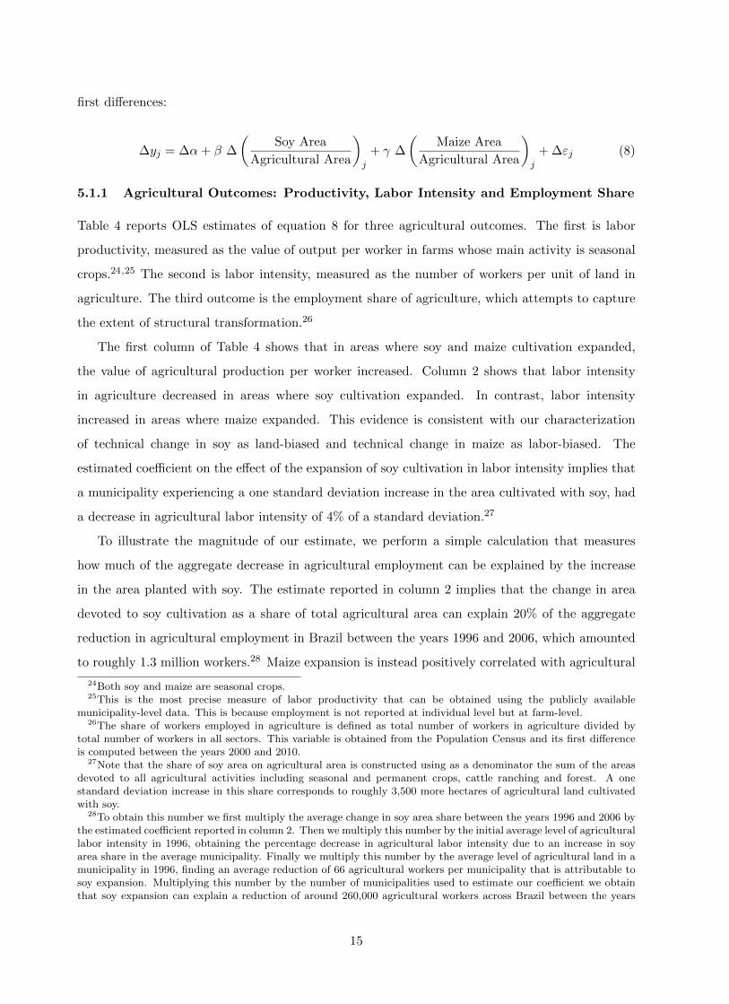
5.1.1 Agricultural Outcomes: Productivity, Labor Intensity and Employment Share

Table 4 reports OLS estimates of equation 8 for three agricultural outcomes. The first is labor

productivity, measured as the value of output per worker in farms whose main activity is seasonal

crops.24,25 The second is labor intensity, measured as the number of workers per unit of land in

agriculture. The third outcome is the employment share of agriculture, which attempts to capture

the extent of structural transformation.26

The first column of Table 4 shows that in areas where soy and maize cultivation expanded,

the value of agricultural production per worker increased. Column 2 shows that labor intensity

in agriculture decreased in areas where soy cultivation expanded. In contrast, labor intensity

increased in areas where maize expanded. This evidence is consistent with our characterization

of technical change in soy as land-biased and technical change in maize as labor-biased. The

estimated coefficient on the effect of the expansion of soy cultivation in labor intensity implies that

a municipality experiencing a one standard deviation increase in the area cultivated with soy, had

a decrease in agricultural labor intensity of 4% of a standard deviation.27

To illustrate the magnitude of our estimate, we perform a simple calculation that measures

how much of the aggregate decrease in agricultural employment can be explained by the increase

in the area planted with soy. The estimate reported in column 2 implies that the change in area

devoted to soy cultivation as a share of total agricultural area can explain 20% of the aggregate

reduction in agricultural employment in Brazil between the years 1996 and 2006, which amounted

to roughly 1.3 million workers.28 Maize expansion is instead positively correlated with agricultural

24Both soy and maize are seasonal crops.25This is the most precise measure of labor productivity that can be obtained using the publicly available

municipality-level data. This is because employment is not reported at individual level but at farm-level.26The share of workers employed in agriculture is defined as total number of workers in agriculture divided by

total number of workers in all sectors. This variable is obtained from the Population Census and its first differenceis computed between the years 2000 and 2010.

27Note that the share of soy area on agricultural area is constructed using as a denominator the sum of the areasdevoted to all agricultural activities including seasonal and permanent crops, cattle ranching and forest. A onestandard deviation increase in this share corresponds to roughly 3,500 more hectares of agricultural land cultivatedwith soy.

28To obtain this number we first multiply the average change in soy area share between the years 1996 and 2006 bythe estimated coefficient reported in column 2. Then we multiply this number by the initial average level of agriculturallabor intensity in 1996, obtaining the percentage decrease in agricultural labor intensity due to an increase in soyarea share in the average municipality. Finally we multiply this number by the average level of agricultural land in amunicipality in 1996, finding an average reduction of 66 agricultural workers per municipality that is attributable tosoy expansion. Multiplying this number by the number of municipalities used to estimate our coefficient we obtainthat soy expansion can explain a reduction of around 260,000 agricultural workers across Brazil between the years

15

labor intensity. The estimated coefficient on the effect of the expansion of maize cultivation in

labor intensity implies that a municipality experiencing a 1 standard deviation increase in the area

cultivated with maize, had an increase in agricultural labor intensity of around 10% of a standard

deviation.

Finally, column 3 shows that the employment share of agriculture decreased in places where

soy expanded. In contrast, the employment share of agriculture increased in areas where maize

expanded, although this change is not statistically significant.

5.1.2 Manufacturing Outcomes: Employment Share, Total Employment and Wages

We now turn to the question of whether manufacturing employment expanded (contracted) in areas

where soy (maize) expanded. Table 5 reports OLS estimates of equation 8 for three manufacturing

outcomes: manufacturing employment share, the level of employment in manufacturing, and the

average wage in the manufacturing sector.

Note that the timing of Population and Agricultural Censi do not coincide, thus our estimation

of equation (8) relates changes in manufacturing outcomes between 2000 and 2010 to changes in the

area planted with soy and maize between 1996 and 2006. In both cases the initial year precedes the

timing of legalization of soybean seeds in Brazil (2003), as well as the first date in which smuggling

of GE soy seeds was documented (2001).

The first column of Table 5 shows that municipalities where soy expanded experienced a faster

increase in the employment share in manufacturing. In contrast, this share remained unchanged

in municipalities where maize expanded. The estimated coefficient on the effect of the expansion

of soy cultivation in manufacturing employment share implies that a municipality experiencing a 1

standard deviation increase in the area cultivated with soy had an increase in the manufacturing

employment share of 7% of a standard deviation. Interestingly, in areas where soy expanded, not

only the share but also the level of manufacturing employment increased, as shown in column 2.

To illustrate the magnitude of our estimate, we perform a simple calculation that measures how

much of the aggregate increase in manufacturing employment can be explained by the expansion

in the area planted with soy. The estimate reported in column 2 implies that the change in area

devoted to soy cultivation as a share of total agricultural area can explain 6% of the aggregate

increase in manufacturing employment in Brazil between the years 2000 and 2010, which amounted

to roughly 1.6 million workers in the sample used to estimate our coefficient.29 The last column

1996 and 2006.29To obtain this number we first multiply the average change in soy area share between the years 1996 and 2006 by

the estimated coefficient reported in column 2. Then we multiply this number by the initial average level of manufac-turing employment across municipalities in 1996, finding an average increase of around 24 manufacturing workers per

16

of Table 5 reports estimated coefficients of the correlation between the expansion in soy and maize

area and wages in manufacturing, which are both not statistically different from zero.

The finding that manufacturing employment increased in areas where soy expanded suggests

that soy technical change is not only land-biased but also strongly labor-saving. In this case, our

model predicts that technology adoption reduces labor demand in agriculture inducing a reallocation

of labor towards manufacturing.

5.2 The Effect of Agricultural Technological Change on Structural Transforma-

tion

In this section we provide direct empirical evidence on the causal effects of the widespread adoption

of new agricultural technologies on industrial development in Brazil. The basic correlations in the

data reported in the previous section show that areas where soy expanded experienced an increase

in output per worker and a reduction in labor intensity in agriculture while industrial employment

expanded. However, these correlations are not informative about the direction of causality. Indeed,

these findings could reflect the two following different sequences of events. First, the adoption of

strongly labour saving agricultural technologies reduces labor demand in the agricultural sector

and induces a reallocation of labor towards the industrial sector. Second, productivity growth in

the industrial sector increases labor demand and wages, inducing agricultural firms to switch to

less labor-intensive crops, like soy. To establish the direction of causality we exploit the timing of

adoption and the differential impact of the new technology on potential yields across geographical

areas.

First, we discuss the timing of adoption. GE soy seeds were patented in the U.S. in 1996, and

legalized in Brazil in 2003. Given that GE seeds were developed in the U.S., their date of invention,

1996, is exogenous with respect to developments in the Brazilian economy. In contrast, the date

of legalization, 2003, responded partly to pressure from Brazilian farmers. In addition, smuggling

of GE soy seeds across the border with Argentina is reported since 2001. Thus, in our empirical

analysis we will compare outcomes before and after 1996 whenever possible.30 The cultivation

techniques necessary to introduce the second harvest maize, instead, were developed within Brazil.

Thus, the timing of its expansion can not be considered exogenous to other developments in the

Brazilian economy. Nevertheless, since the diffusion of this new technology across space depends

municipality that is attributable to soy expansion. Multiplying this number by the number of municipalities used toestimate our coefficient we obtain that soy expansion can explain an increase of around 92,000 manufacturing workersacross Brazil between the years 1996 and 2006.

30For some data sources we will compare outcomes before and after 2001 or 2003, due to data availability constraints.In those cases, however, the potential effect of smuggling can only bias downward our estimates.

17

on exogenous local soil and weather characteristics, we think it is reasonable to argue that this

diffusion is exogenous to developments in the local industrial sector.

Second, these new technologies have a differential impact on potential yields depending on soil

and weather characteristics. Thus, we exploit these exogenous differences on potential yields across

geographical areas as our source of cross-sectional variation in the intensity of the treatment.

To implement this strategy, we need an exogenous measure of potential yields for soy and

maize, which we obtain from the FAO-GAEZ database. These potential yields are estimated by

FAO using an agricultural model that predicts yields for each crop given climate and soil conditions.

As potential yields are a function of weather and soil characteristics, not of actual yields in Brazil,

they can be used as a source of exogenous variation in agricultural productivity across geographical

areas. Crucially for our analysis, the database reports potential yields under different technologies or

input combinations. Yields under low inputs are described as those obtained using traditional seeds

and no use of chemicals, while yields under high inputs are obtained using high yielding varieties

and optimum application of fertilizers and herbicides. Thus, the difference in yields between the

high and low technology captures the effect of moving from traditional agriculture to a technology

that uses optimum weed control, among other characteristics.31 We expect this increase in yields

to be a good predictor of the profitability of adopting herbicide resistant GE soy seeds.

More formally, our basic empirical strategy consists in estimating the following equation:

yjt = αj + αt + β Asoyjt + εjt (9)

where yjt is an outcome that varies across municipalities and time, j indexes municipalities, t

indexes time, αj are municipality fixed effects, αt are time fixed effects and Asoyjt is equal to the

potential soy yield under high inputs from 2003 onwards and to the potential soy yield under low

inputs in the years before 2003. Asoyjt can be thought of as the empirical counterpart of the labor

augmenting technical change AL presented in our model.

In the case of maize, we follow a similar strategy. As noted in Section 2, the cultivation of second

harvest maize requires the use of modern techniques that are intensive in the use of fertilizers,

herbicides and tractors. Thus, we expect that the the difference in FAO-GAEZ potential yields

31The description of each technology in the FAO-GAEZ dataset documentation is as follows. Low-level in-puts/traditional management: ”Under the low input, traditional management assumption, the farming system islargely subsistence based and not necessarily market oriented. Production is based on the use of traditional cultivars(if improved cultivars are used, they are treated in the same way as local cultivars), labor intensive techniques, andno application of nutrients, no use of chemicals for pest and disease control and minimum conservation measures.”High-level inputs/advanced management: ”Under the high input, advanced management assumption, the farmingsystem is mainly market oriented. Commercial production is a management objective. Production is based on im-proved high yielding varieties, is fully mechanized with low labor intensity and uses optimum applications of nutrientsand chemical pest, disease and weed control.”

18

between the high and low technology captures the profitability of planting second season maize.

Thus, we augment the equation described above to include the following variable: Amaizejt which

is equal to the potential maize yield under high inputs from 2003 onwards and to the potential

maize yield under low inputs in the years before 2003. Amaizejt can be thought of as the empirical

counterpart of the land augmenting technical change AT presented in our model.

yjt = αj + αt + βAsoyjt + γAmaize

jt + εjt . (10)

In the following subsections we report the results of using our measure of technical change to

explain changes in agricultural production and in the sectoral composition of the economy. Section

5.2.1 reports the relationship between our measure of technical change and the expansion of soy and

maize cultivation. Section 5.2.2 shows the relationship between this measure and other agricultural

outcomes. Finally, section 5.2.3 presents results using manufacturing outcomes.

5.2.1 Agricultural Outcomes: Soy and Maize Expansion

In this section we document the relationship between technical change measured by the increase

in the FAO-GAEZ potential yield of soy and maize, and the actual change in agricultural area

cultivated with each crop. The objective of this exercise is to check whether the change in potential

yields is a good proxy of the profitability of the adoption of new agricultural technologies. If this is

the case, we expect the increase in the potential yield of a given crop to predict the actual expansion

in the area cultivated with that crop between 1996 and 2006. With this purpose, we estimate a

first-difference version of equation 10:

∆yj = ∆α+ β∆Asoyj + γ∆Amaize

j + ∆εj (11)

where the outcome of interest, ∆yj is the change in share of farm land reaped with either soy or

maize between 1996 and 2006, and Asoyj is potential yield of soy under high inputs minus potential

yields of soy under low inputs (Asoyj is its equivalent for maize).

Column 1 in Table 6 shows that the increase in potential soy yield predicts the expansion

in soy area as a share of agricultural area between 1996 and 2006. Column 2 shows that this

estimate is robust to controlling for the increase in potential maize yield. The size of the estimated

coefficient reported in column 3 implies that a one standard deviation increase in potential soy

yield corresponds to an increase in the share of soy in agricultural land of almost 30% of a standard

deviation. Notice also that the estimated effect of the increase in potential maize yield on the

expansion of soy area is negative and statistically significant.

19

Similarly, the estimates reported in column 3 imply that the increase in potential maize yield

predicts the expansion in maize area as a share of agricultural area between 1996 and 2006. Column

4 shows that this estimate is robust to controlling for the increase in potential soy yield, which in

turn has a negative effect on the expansion of maize area as a share of agricultural area. The size

of the estimated coefficient implies that a one standard deviation increase in potential maize yield

corresponds to an increase in the share of maize in agricultural area of 14% of a standard deviation.

The fact that our measure of technical change correctly predicts the expansion or retrenchment

of specific crops suggests that it captures the benefits of adoption of new agricultural technologies.

Taken together, the results reported in Table 6 suggest that technical change measured as the

increase in a crop potential yield had large effects on land allocation.

Next, we investigate whether the expansion in soy area is driven by the adoption of GE soy.

For this purpose, we check whether our measure of technical change in soy predicts actual adoption

of GE seeds.32 In principle, we expect that areas with a higher increase in FAO-GAEZ potential

soy yields are those switching to genetically engineered soy on a larger scale. Column 1 of Table 7

shows that this is indeed the case. The size of the estimated coefficient implies that a one standard

deviation increase in potential soy yield corresponds to an increase in GE soy area as a share of

agricultural area of 25% of a standard deviation. In column 2 we perform a falsification test, by

looking at the correlation between the change in potential soy yield and the expansion in non-GE

soy area. In this case, the coefficient is negative and significant. This finding suggests that the

change in potential soy yield correctly captures the benefits of adopting GE soy vis-a-vis traditional

soy seeds.

5.2.2 Agricultural Outcomes: Productivity, Labor Intensity and Employment Share

In this section we study the effect of agricultural technical change on production and employment in

agriculture. Table 8 reports the results of estimating equation (11) where the dependent variables

are three agricultural outcomes: the value of agricultural production per worker in seasonal crops,

labor intensity, and the share of workers employed in agriculture, all defined as in section 5.1.1.

The estimated coefficients reported in column 1 of Table 8 indicate that in areas where the

potential soy yield increased relatively more, the value of agricultural production per worker in-

creased. The size of the estimated coefficient implies that a one standard deviation increase in

potential soy yield corresponds to an increase in the value of agricultural production per worker

of 7% of a standard deviation. On the other hand, an increase in potential maize yield seems

32Unfortunately, we can not perform the same test for maize given that the publicly available Agricultural Censusdata does not contain information on the season of planting of maize at the municipality level.

20

negatively associated with the value of agricultural production per worker, but this effect is not

statistically significant.

The estimated coefficients reported in column 2 indicate that in areas where potential soy yield

increased relatively more, agricultural labor intensity decreased. The size of the coefficient implies

that a one standard deviation increase in potential soy yield corresponds to a decrease in the ratio

of workers per unit of land in agriculture of 5% of a standard deviation. In contrast, the estimated

coefficient of the increase in potential maize yield is positive and significant, indicating that in

areas where potential maize yield increased relatively more agricultural labor intensity increased.

The size of the coefficient implies that a one standard deviation increase in potential maize yield

corresponds to an increase in agricultural labor intensity of 8% of a standard deviation. Notice

that the effects of potential soy and maize yields on labor intensity in agriculture are consistent

with the correlations presented in section 5.1.1.

Finally, the estimated coefficients reported in column 3 suggest that an increase in the potential

soy yield have no statistically significant effect on agricultural employment share. Note that these

results contrast with the simple correlations in the data reported in section 5.1.1, according to

which areas where soy expanded experienced a reduction in the employment share in agriculture.

This inconsistency might respond to two causes. First, potential soy yields are estimated, thus they

might not correctly capture the benefits of GE soy adoption. Second, the agricultural employment

share is measured with error in the Population Census. Individuals interviewed for the Brazilian

Population Census are classified in different sectors depending on the occupation they report in the

week preceding the interview. This is a potential problem when measuring employment, especially

in agriculture, where employment is more seasonal than in other sectors.

Taken together, the results presented in Table 8 suggest that the introduction of new agricultural

technologies in Brazil had a sizable impact in agricultural labor markets. Areas where the potential

impact of GE soy adoption was higher experienced an increase in the value of agricultural production

per worker and a reduction in the number of workers per unit of land. These findings are consistent

with our characterization of the adoption of GE soy as a land-biased technical change. In the case of

maize, areas where the potential impact of the introduction of a second harvesting season was higher

experienced an increase in the number of workers per unit of land. This result is also consistent

with our characterization of the introduction of a second harvesting season as labor-biased technical

change.

21

5.2.3 Manufacturing Outcomes: Employment Share, Employment and Wages

In this section we study the effect of agricultural technical change on manufacturing employment

and wages. Table 9 reports the results of estimating equation (11) where the dependent variables are

three manufacturing outcomes: the employment share of manufacturing, the level of manufacturing

employment, and the average wage in manufacturing as defined in section 5.1.2.

The estimates reported in column 1 indicate that areas where potential soy yield increased

relatively more, experienced a larger increase in the employment share of manufacturing. The size

of the estimated coefficient implies that a one standard deviation increase in potential soy yield

corresponds to an increase in manufacturing employment share of 30% of a standard deviation. On

the other hand, areas with higher increase in potential maize yield experienced a larger decrease

in the manufacturing employment share. . The size of the estimated coefficient implies that a one

standard deviation increase in potential maize yield corresponds to a decrease in manufacturing

employment share of 12% of a standard deviation.

When looking at the level of manufacturing employment instead of its share in total employ-

ment we find very similar results. The estimates reported in column 2 suggest that areas where

potential soy yield increased relatively more, experienced a larger increase in the level of manu-

facturing employment. The estimated coefficient implies that a one standard deviation increase in

potential soy yield corresponds to an increase in the level of manufacturing employment of 34% of a

standard deviation. Again, we observe the opposite result for the potential maize yield: areas with

higher increase in potential maize yield experienced a larger decrease in the level of manufacturing

employment. The size of the estimated coefficient is such that one standard deviation increase in

potential maize yield corresponds to a decrease in the level of manufacturing employment of almost

20% of a standard deviation.

Finally, we study the effect of potential soy and maize yields on manufacturing wages. The

results reported in column 3 indicate that areas where potential soy yields increased relatively

more, experienced a larger decrease in average manufacturing wages. The estimated coefficient

implies that a one standard deviation increase in potential soy yields corresponds to a decrease in

average manufacturing wages of 16% of a standard deviation. An increase in potential maize yield

has the opposite effect on manufacturing wages: in areas where potential maize yield increased

relatively more, average manufacturing wages also increased (15% of a standard deviation for a one

standard deviation increase in potential maize yield).

Taken together, the estimates reported in this section are consistent with the empirical pre-

dictions of our model. They show that the effects of agricultural productivity on the industrial

22

sector depend on the factor bias of technical change. In the case of soy, our estimates indicate that

strongly labor saving technologies (like GE seeds), by reducing the demand for labor in agriculture,

promote the growth of the manufacturing sector through an increase in labor supply and lower

wages. On the other hand, in the case of maize, our estimates show that land-augmenting technical

change (like the introduction of a second harvesting season), by increasing the labor intensity of

agriculture, result in a decrease of manufacturing employment and increasing wages.

6 Robustness Checks

6.1 Robustness to Using a Larger Unit of Observation: Micro-Regions

In the empirical analysis performed so far we assumed that municipalities are the best approxima-

tion of the relevant labor market faced by Brazilian agricultural workers. A potential issue is that

local labor market boundaries do not overlap with a municipality’s administrative boundaries. In

particular, some municipalities might be too small to properly capture labor flows between urban

and rural areas, provided manufacturing activities take place in the former, and agricultural activ-

ities in the latter. In order to take into account this concern we aggregate our data at a larger unit

of observation: the micro-regions. Table 10 and 11 show that the results reported in Tables 5 and

9 are robust to using the 557 micro-regions for which data are available as units of observation.

6.2 Falsification Test: Checking for Pre-Existing Trends

In this section we address the possibility that our results are driven by pre-existing trends. If

municipalities with the largest increase in potential soy and maize yields were already experiencing

faster structural transformation before 2000, the results shown in the previous section may not be

caused entirely by the technical changes introduced by GE soy seeds and the second harvesting

season in maize.

Table 12 reports the results of our falsification test. We replicate the estimation of equation

11 as reported in Table 9 but using differences in manufacturing outcomes between 1991 and 2000

instead of between 2000 and 2010. We perform this test for manufacturing employment and average

manufacturing wages but not for the manufacturing employment share on total employment that we

are unable to measure consistently across the 1991 and 2000 censi due to a change in the definition

of employment introduced by the IBGE after the 1991 Census.33

33Between the 1991 and 2000 censi the Brazilian Statistical Institute (IBGE) changed its definition of employmentin two important ways. First, it started to count zero-income workers as employed. In order to homogenize theBrazilian Census with international practices, the IBGE started to consider employed anyone who helped anotherhousehold member with no formal compensation, as well as agricultural workers that produced only for their own

23

Table 12 shows that that our measures of technical change in agriculture do not explain variation

in manufacturing employment or wages before 2000. The estimated coefficients on potential soy and

maize yields are not statistically different from zero. The only exception is the estimated coefficient

of potential maize yield on wages in column 2, which is positive and marginally significant.34 This

falsification test validates our interpretation that the effect of our measures of technical change on

structural transformation is due to the introduction of new agricultural technologies rather than to

pre-existing trends in the areas that were mostly affected by these new technologies.

6.3 Robustness to Controlling for Commodity Prices

Another potential concern is that our results might be driven by the evolution of commodity prices,

soy and maize in particular, and not by technical change. For example, an increase in the price

of soy could induce an expansion in the area planted with this crop and generate income spent

on manufacturing goods produced in the same area. The evolution of international prices for soy

and maize is depicted in Figures 14 and 15. Both soy and maize prices are relatively stable in

the period 1996-2006, and they both start growing from 2007. Thus, throughout the period of

analysis for agricultural variables (1996-2006) prices were relatively stable. Still, the period of

analysis of manufacturing variables (2000-2010) includes these years of high prices. This is in

principle problematic because, although international commodity prices should affect all Brazilian

municipalities at the same time, they might still have heterogeneous effects in places that are more

suitable to the cultivation of a particular crop.

To address this concern, we use an alternative source of data on manufacturing employment

that, unlike the Population Census, has a yearly frequency. This permits to both exclude the years

where prices are high from the analysis and fully control for yearly prices.

The source of these data is the yearly industry survey (PIA), which covers the universe of firms

consumption (IBGE, 2003; p. 218). Zero-income workers are more common in agriculture than in other sectors, andin 1991 were only partially included in the labor force. In the 1991 Census 15% of agricultural workers reported zeroincome, against 34% in 2000 and 35% in 2010 (the corresponding numbers for people employed in fishery are 3%in 1991, 22% in 2000 and 28% in 2010). Second, the IBGE changed the reference period for considering a personemployed: while in 1991 such period included the last 12 months, in 2000 it only included the reference week of theCensus. This new rule implied that workers performing temporary and seasonal activities that were not employedduring the reference week were counted in the 1991 census but not the in the 2000 census. The IBGE felt thatinquiring into temporary employment entailed too many additional questions, and that smaller surveys would bemore suitable to deal with the matter (IBGE, 2003; p. 218). Also this second change is likely to be especiallyproblematic for the agricultural sector, also considering that the reference week in the 2000 Census was in the middleof the Brazilian winter. This is why, to test for pre-existing trends, we focus on the absolute number of workersemployed in manufacturing as an outcome (instead of its share in total employment). This measure is less likely tobe affected by the changes introduced between the two censi, because: (1) there are virtually no zero-income workersin manufacturing (only 0.5%, 1.9% and 1% of manufacturing workers declare zero income in 1991, 2000 and 2010,respectively) and (2) manufacturing is less seasonal than other sectors.

34This could reflect the fact that a second harvesting season for maize was introduced in several areas of Brazilalready before 2000.

24

with at least 30 employees in Brazil and it is therefore, for this class of firms, representative at

municipality level. We focus on two variables from this survey: total manufacturing employment

and average wage.35

We estimate an equation of the following form:

yjt = αj + αt + βAsoyjt + γAmaize

jt +∑z

θzPzt A

zj0 + εjt (12)

where yjt is total employment or average wage in a given municipality; Asoyjt is equal to the potential

soy yield under low inputs for all years before 2003 and to the potential soy yield under high inputs

starting from 2003 (same criteria is used to define Amaizejt ). We observe all years from 1996 to 2006

and control for the prices of soy and maize multiplied by the potential yield under low inputs of

these crops. In all specifications we control for both municipality and year fixed effects (αj and αt)

and cluster standard errors at the municipality level to address potential serial correlation in the

error term (Bertrand, et al., 2004).

The results obtained using data from the industrial survey are consistent with those obtained

using the Population Census data (see Table 9): areas where potential soy yields increased rela-

tively more, experienced a larger increase in manufacturing employment and a larger decrease in

average manufacturing wages. To compare the magnitude of the estimated coefficients with those

obtained using the Population Census data we calculate how much of the change in manufactur-

ing employment and wages between the years 1996 and 2006 can be explained by the change in

potential soy and maize yields in the same years. The estimated coefficients in column 2 and 4

imply that a one standard deviation increase in potential soy yield corresponds to an increase in

manufacturing employment of 6% of a standard deviation and a decrease in average manufacturing

wages of 6% of a standard deviation. An increase in potential maize yield has instead the opposite

effect when the outcome is the average manufacturing wage (6.5% of a standard deviation for a one

standard deviation increase in potential maize yield) while its effect is negative but not statistically

significant when the outcome is total manufacturing employment.36

35The average wage is defined as the aggregate wage bill (in real terms) divided by the total number of workersemployed in a municipality.

36The fact that these effects are quantitatively smaller with respect to those obtained with the Population Censuscan be attributed to the following reasons: (1) the yearly industrial survey, differently from the Population Census,does not cover informal employment (2) the changes in manufacturing employment and wages in the PopulationCensus are calculated between the years 2000 and 2010, while in the industrial survey they are calculated betweenthe years 1996 and 2006 (i.e. this data covers a shorter period after the introduction of the new technology), (3) theindustrial survey tends to over represent larger firms that are more likely to hire high skilled workers with respect tolow skilled workers, and are therefore less likely to be hiring former agricultural workers.

25

7 Final Remarks

The process of modern economic growth is accompanied by structural transformation, i.e. the

reallocation of economic activity from agriculture to industry. Identifying the forces behind struc-

tural transformation is therefore key to our understanding of economic development. Based on

the experience of England during the industrial revolution, economists have argued that increases

in agricultural productivity is one important force behind structural transformation. However, as

underlined by Matsuyama (1992), in open economies a comparative advantage in agriculture could

instead slow down industrial growth. Despite the importance of the question, there is so far scarce

evidence on the channels through which agricultural productivity can shape the reallocation of

economic activity across sectors in an open economy.

In this paper we argue that the effect of agricultural productivity on industrial development

depends crucially on the factor-bias of technical change. In particular, predictions of models of

structural transformation in open economies hold when technical change is hicks neutral or labor-

biased, but are reversed when land-biased technical change is strongly labor saving.

We provide direct empirical evidence on these mechanisms by isolating the effects of adoption

of two new agricultural technologies in Brazil: genetically engineered soybean seeds and a second

harvesting season for maize. We argue that the first technical change is land-biased, while the

second is labor-biased, and exploit this setup to study the effect of the diffusion of these agricultural

technologies on the manufacturing sector. To identify the causal effects of this new technology, we

exploit the timing of adoption and the differential impact of the new technologies on potential

yields across geographical areas.

We find that in municipalities where the new technology had a larger potential impact on

soy yields, there was faster GE soy adoption, a reduction of labor intensity in agriculture and an

expansion of manufacturing employment. In contrast, in municipalities where the new technology

had a larger potential impact on maize yields, there was an increase of labor intensity in agriculture

and a contraction of manufacturing employment. These different effects documented for soy and

maize indicate that the factor bias of technical change is a key factor in the relationship between

agricultural productivity and industrial growth in open economies.

26

References

Acemoglu, D. (2010). “When Does Labor Scarcity Encourage Innovation?”. Journal of PoliticalEconomy 118, 1037–1078.

Acemoglu, D. and V. Guerrieri (2008). “Capital Deepening and Non-Balanced Economic Growth”.Journal of Political Economy 116, 467–498.

Baumol, W. J. (1967). “Macroeconomics of Unbalanced Growth: the Anatomy of Urban Crisis”.American Economic Review 57 (3), 415–426.

Bertrand, M., E. Duflo, and S. Mullainathan (2004). “How Much Should We Trust Differences-in-differences Estimates?”. Quarterly Journal of Economics 119 (1), 249–275.

Buera, F. J. and J. P. Kaboski (2009). “Can Traditional Theories of Structural Change Fit theData?”. Journal of the European Economic Association 7 (2-3), 469–477.

Caselli, F. and W. J. Coleman II (2001). “The US Structural Transformation and Regional Con-vergence: A Reinterpretation”. Journal of Political Economy 109 (3), 584–616.

Clark, C. (1940). “The Conditions of Economic Progress”. London: MacMillan & Co.

CONAB (2003-2012). “Levantamento De Avaliacao Da Safra”.

Duffy, M. and D. Smith (2001). “Estimated Costs of Crop Production in Iowa”. Iowa StateUniversity Extension Service FM1712.

EMBRAPA (2006). “Cultivo do Milho”. Embrapa, Sistemas de Producao.

Fajgelbaum, P., G. M. Grossman, and E. Helpman (2011). “Income Distribution, Product Quality,and International Trade”. Journal of Political Economy 119 (4), 721–765.

Fernandez-Cornejo, J. and M. Caswell (2006). “The First Decade of Genetically Engineered Crops inthe United States”. United States Department of Agriculture, Economic Information Bulletin 11.

Fernandez-Cornejo, J., C. Hendricks, and A. Mishra (2005). “Technology Adoption and Off-FarmHousehold Income: The Case of Herbicide-Tolerant Soybeans”. Journal of Agricultural andApplied Economics 37 (3), 549.

Fernandez-Cornejo, J., C. Klotz-Ingram, and S. Jans (2002). “Estimating Farm-Level Effects ofAdopting Herbicide-Tolerant Soybeans in the USA”. Journal of Agricultural and Applied Eco-nomics 34, 149–163.

Field (1978). “Sectoral Shifts in Antebellum Massachusetts: A Reconsideration”. Exploration inEconomic History 15, 146–171.

Foster, A. D. and M. R. Rosenzweig (2004). “Agricultural Productivity Growth, Rural EconomicDiversity, and Economic Reforms: India, 1970–2000”. Economic Development and CulturalChange 52 (3), 509–542.

Foster, A. D. and M. R. Rosenzweig (2008). “Economic Development and the Decline of AgriculturalEmployment”. Handbook of Development Economics 4, 3051–3083.

Gollin, D., S. Parente, and R. Rogerson (2002). “The Role of Agriculture in Development”. Amer-ican Economic Review 92 (2), 160–164.

27

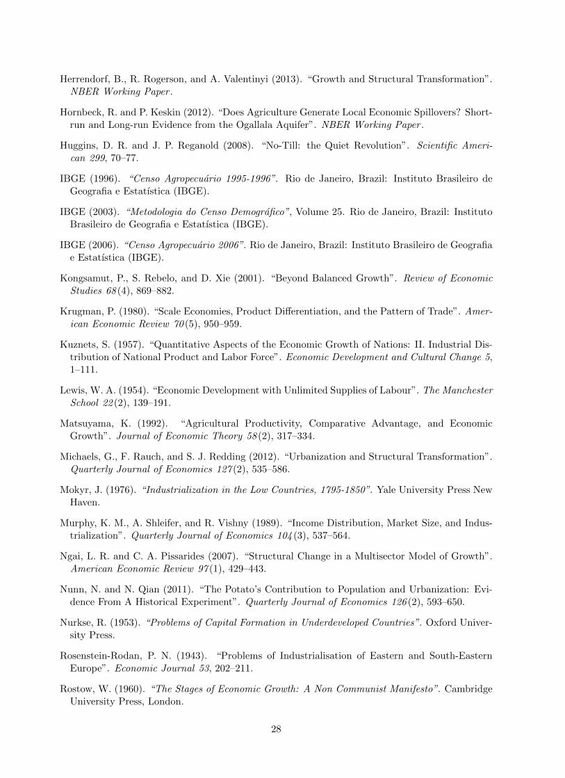
Herrendorf, B., R. Rogerson, and A. Valentinyi (2013). “Growth and Structural Transformation”.NBER Working Paper .

Hornbeck, R. and P. Keskin (2012). “Does Agriculture Generate Local Economic Spillovers? Short-run and Long-run Evidence from the Ogallala Aquifer”. NBER Working Paper .

Huggins, D. R. and J. P. Reganold (2008). “No-Till: the Quiet Revolution”. Scientific Ameri-can 299, 70–77.

IBGE (1996). “Censo Agropecuario 1995-1996”. Rio de Janeiro, Brazil: Instituto Brasileiro deGeografia e Estatıstica (IBGE).

IBGE (2003). “Metodologia do Censo Demografico”, Volume 25. Rio de Janeiro, Brazil: InstitutoBrasileiro de Geografia e Estatıstica (IBGE).

IBGE (2006). “Censo Agropecuario 2006”. Rio de Janeiro, Brazil: Instituto Brasileiro de Geografiae Estatıstica (IBGE).

Kongsamut, P., S. Rebelo, and D. Xie (2001). “Beyond Balanced Growth”. Review of EconomicStudies 68 (4), 869–882.

Krugman, P. (1980). “Scale Economies, Product Differentiation, and the Pattern of Trade”. Amer-ican Economic Review 70 (5), 950–959.

Kuznets, S. (1957). “Quantitative Aspects of the Economic Growth of Nations: II. Industrial Dis-tribution of National Product and Labor Force”. Economic Development and Cultural Change 5,1–111.

Lewis, W. A. (1954). “Economic Development with Unlimited Supplies of Labour”. The ManchesterSchool 22 (2), 139–191.

Matsuyama, K. (1992). “Agricultural Productivity, Comparative Advantage, and EconomicGrowth”. Journal of Economic Theory 58 (2), 317–334.

Michaels, G., F. Rauch, and S. J. Redding (2012). “Urbanization and Structural Transformation”.Quarterly Journal of Economics 127 (2), 535–586.

Mokyr, J. (1976). “Industrialization in the Low Countries, 1795-1850”. Yale University Press NewHaven.

Murphy, K. M., A. Shleifer, and R. Vishny (1989). “Income Distribution, Market Size, and Indus-trialization”. Quarterly Journal of Economics 104 (3), 537–564.

Ngai, L. R. and C. A. Pissarides (2007). “Structural Change in a Multisector Model of Growth”.American Economic Review 97 (1), 429–443.

Nunn, N. and N. Qian (2011). “The Potato’s Contribution to Population and Urbanization: Evi-dence From A Historical Experiment”. Quarterly Journal of Economics 126 (2), 593–650.

Nurkse, R. (1953). “Problems of Capital Formation in Underdeveloped Countries”. Oxford Univer-sity Press.

Rosenstein-Rodan, P. N. (1943). “Problems of Industrialisation of Eastern and South-EasternEurope”. Economic Journal 53, 202–211.

Rostow, W. (1960). “The Stages of Economic Growth: A Non Communist Manifesto”. CambridgeUniversity Press, London.

28

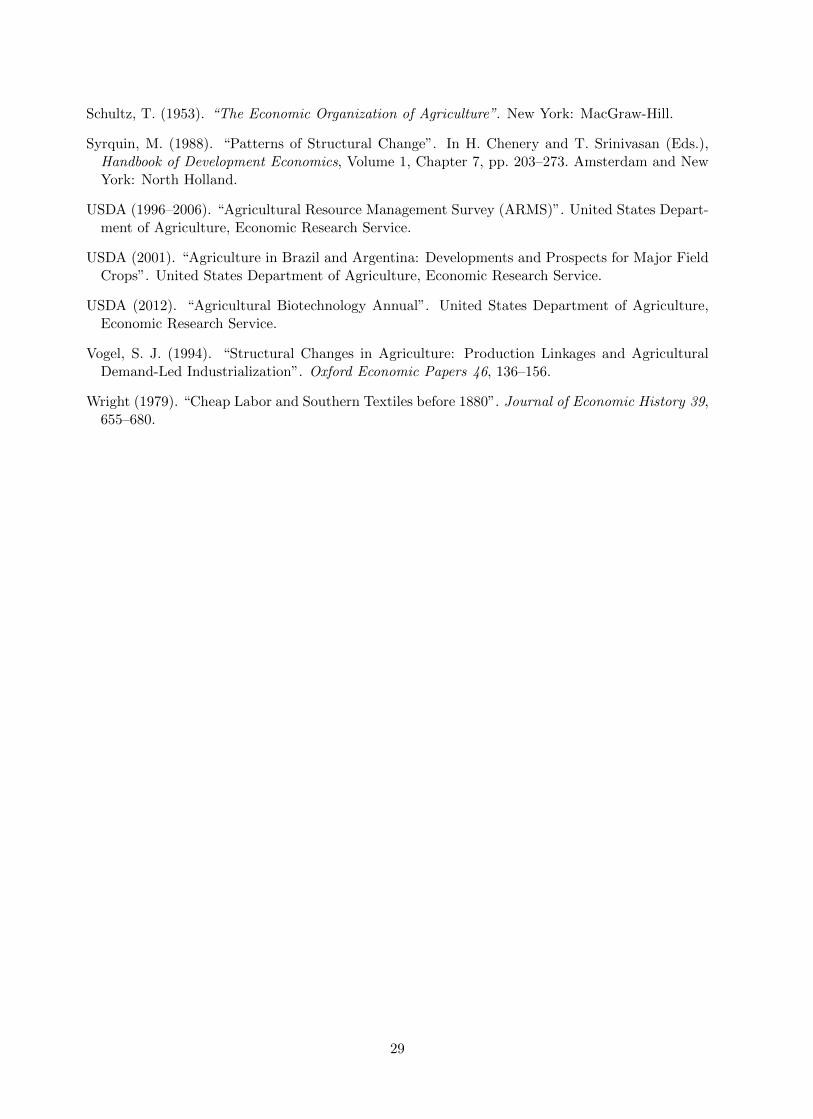
Schultz, T. (1953). “The Economic Organization of Agriculture”. New York: MacGraw-Hill.

Syrquin, M. (1988). “Patterns of Structural Change”. In H. Chenery and T. Srinivasan (Eds.),Handbook of Development Economics, Volume 1, Chapter 7, pp. 203–273. Amsterdam and NewYork: North Holland.

USDA (1996–2006). “Agricultural Resource Management Survey (ARMS)”. United States Depart-ment of Agriculture, Economic Research Service.

USDA (2001). “Agriculture in Brazil and Argentina: Developments and Prospects for Major FieldCrops”. United States Department of Agriculture, Economic Research Service.

USDA (2012). “Agricultural Biotechnology Annual”. United States Department of Agriculture,Economic Research Service.

Vogel, S. J. (1994). “Structural Changes in Agriculture: Production Linkages and AgriculturalDemand-Led Industrialization”. Oxford Economic Papers 46, 136–156.

Wright (1979). “Cheap Labor and Southern Textiles before 1880”. Journal of Economic History 39,655–680.

29

Figures and Tables

Figure 1Employment in agriculture, industry, services and construction(1992-2011)

010

2030

4050

wor

kers

(in

mill

ions

)

1990 1995 2000 2005 2010

year

agriculture manufacturing

services construction

Notes: The Figure shows the evolution between 1992 and 2011 of the total number of workers (expressed

in million) employed by sector in Brazil. The sectors are: Agriculture (codes A and B in the CNAE-

Domiciliar classification), Industry (code D), Services (codes: G, H, I, J , K, L, M , N , O, P , Q, E)

and Construction (code: F ). Workers in the Extractive Industry (code C) are not included in any of

the categories above. Data is from PNAD, a national household survey representative at country level

carried out yearly by the IBGE (the survey was not carried out in 1994 and in the census years: 1991,

2000 and 2010). Since the PNAD coverage changed over time, to harmonize the sample across years we

exclude: (i) workers located in the states of: Rondonia, Acre, Amazonas, Roraima, Para and Amapa

(North macro-region) because only urban areas (and not rural areas) of these states were covered until

2004; (ii) workers located in the states of: Tocantins, Mato Grosso do Sul, Goias and the Distrito Federal

because the sample of households in these states is not complete in the years from 1992 to 1997.

30

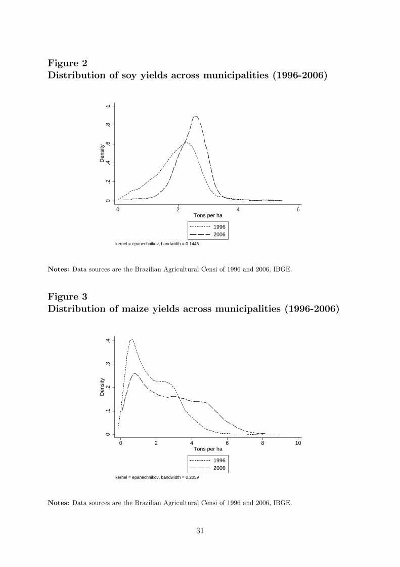
Figure 2Distribution of soy yields across municipalities (1996-2006)

0.2

.4.6

.81

Den

sity

0 2 4 6Tons per ha

19962006

kernel = epanechnikov, bandwidth = 0.1446

Notes: Data sources are the Brazilian Agricultural Censi of 1996 and 2006, IBGE.

Figure 3Distribution of maize yields across municipalities (1996-2006)

0.1

.2.3

.4D

ensi

ty

0 2 4 6 8 10Tons per ha

19962006

kernel = epanechnikov, bandwidth = 0.2059

Notes: Data sources are the Brazilian Agricultural Censi of 1996 and 2006, IBGE.

31

Figure 4Area planted with soy (1980-2011)

510

1520

area

(m

illio

n ha

)

1980 1990 2000 2010

year

Notes: The Figure depicts the evolution between 1980 and 2011 of the total area planted with soy

in Brazil (expressed in million hectares). Data sources are monthly surveys carried out by CONAB,

Companhia Nacional de Abastecimento, an agency created by the Brazilian Ministry of Agriculture.

Data is constructed by interviewing on the ground farmers, agronomists and financial agents in the main

cities of the country.

32

Figure 5Area planted per worker in soy production (1980-2011)

020

4060

8010

0

hect

ares

per

wor

ker

1980 1990 2000 2010

year

Notes: The Figure depicts the evolution between 1980 and 2011 of the area planted with soy divided

by the total number of workers employed in soy production in Brazil. Data sources are CONAB for area

planted with soy and PNAD for the total number of workers in soy production. CONAB, Companhia

Nacional de Abastecimento, is an agency created by the Brazilian Ministry of Agriculture. Data is

constructed by interviewing on the ground farmers, agronomists and financial agents in the main cities of

the country. PNAD is a national household survey representative at country level carried out yearly by

the IBGE (the survey was not carried out in 1994 and in the census years: 1991, 2000 and 2010). Since

the PNAD coverage changed over time, to harmonize the sample across years we exclude: (i) workers

located in the states of: Rondonia, Acre, Amazonas, Roraima, Para and Amapa (North macro-region)

because only urban areas (and not rural areas) of these states were covered until 2004; (ii) workers located

in the states of: Tocantins, Mato Grosso do Sul, Goias and the Distrito Federal because the sample of

households in these states is not complete in the years from 1992 to 1997. We harmonized data from

CONAB with the PNAD coverage such data numerator and denominator are constructed using the same

subset of states.

33

Figure 6Employment in soy production (1980-2011)

100

200

300

400

500

600

700

wor

kers

(in

thou

sand

s)

1980 1990 2000 2010

year

Notes: The Figure depicts the evolution between 1980 and 2011 of the total number of workers employed

in soy production (expressed in thousands) in Brazil. Data source is PNAD, see the Note under Figure

1 for a detailed description.

Figure 7Area planted with maize (1980-2010)

05

1015

area

(m

illio

n ha

)

1980 1985 1990 1995 2000 2005 2010

year

Total 1st season

2nd season

Notes: The Figure depicts the evolution between 1980 and 2010 of the area planted with maize in

Brazil (expressed in million hectares). The series show the total area planted with maize as well as the

breakdown by the season of harvest (1st or 2nd season). Data sources are monthly surveys carried out

by CONAB, Companhia Nacional de Abastecimento, an agency created by the Brazilian Ministry of

Agriculture.

34

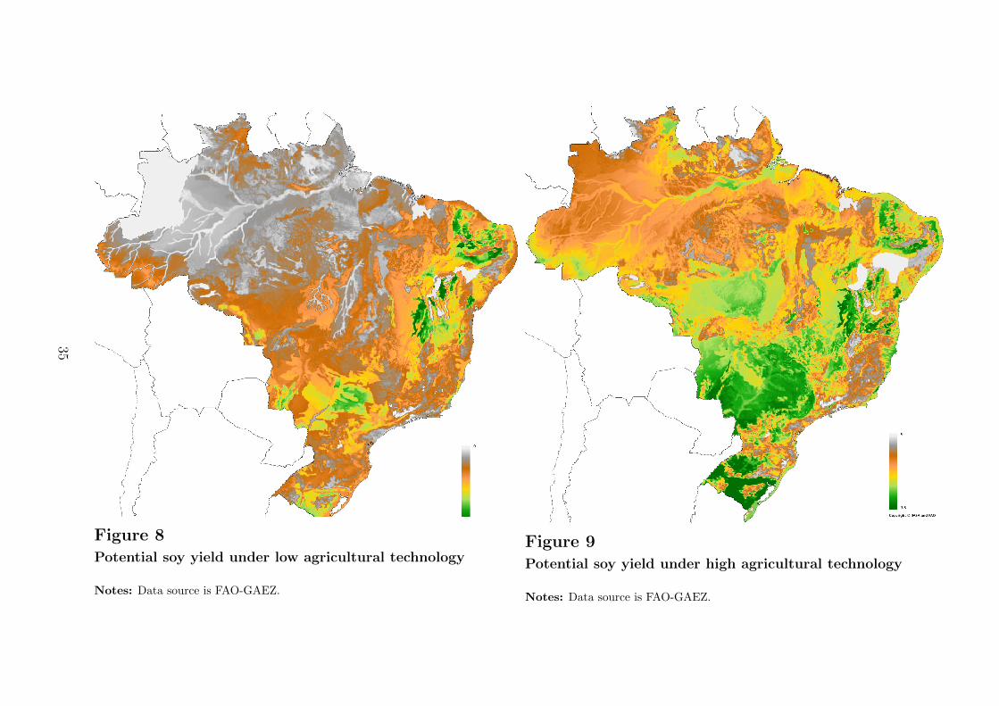
Figure 8Potential soy yield under low agricultural technology

Notes: Data source is FAO-GAEZ.

Figure 9Potential soy yield under high agricultural technology

Notes: Data source is FAO-GAEZ.

35

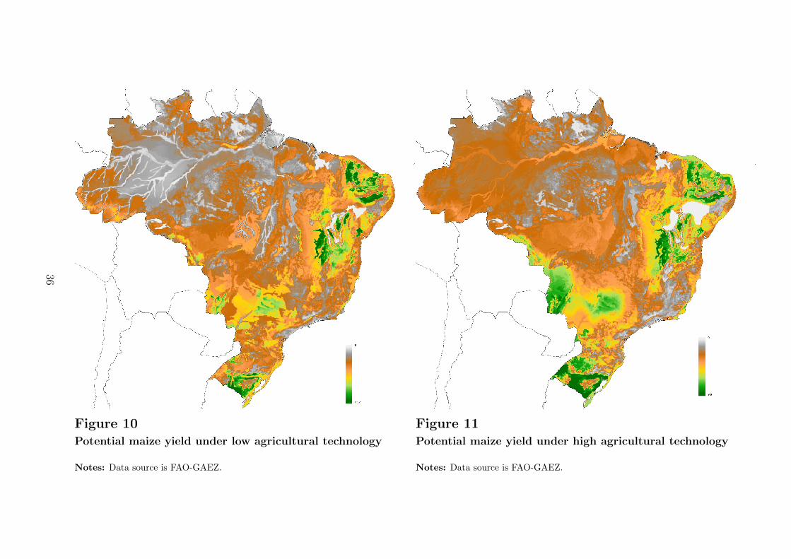
Figure 10Potential maize yield under low agricultural technology

Notes: Data source is FAO-GAEZ.

Figure 11Potential maize yield under high agricultural technology

Notes: Data source is FAO-GAEZ.

36

Figure 12Technological change in soyPotential yield under high technology minus potential yield

under low technology

Municipalities

Notes: Authors’ calculations from FAO-GAEZ data.

Figure 13Technological change in soyPotential yield under high technology minus potential yield

under low technology

Micro-regions

Notes: Authors’ calculations from FAO-GAEZ data.

37

100

200

300

400

500

Soy

bean

s, 2

000

US

$ pe

r m

etric

ton

1990

1992

1994

1996

1998

2000

2002

2004

2006

2008

2010

2012

2014

time

Figure 14Evolution of soy price (1990-2013)

Notes: The Figure shows the monthly evolution of soy real price between 1990

and 2013. Data are from the IMF Primary Commodity Prices database, series

code: PSOYB USD, expressed in nominal US$ per metric ton. We deflate the

series using the US Consumer Price Index for All Urban Consumers: All

Items, source: Federal Reserve St. Louis, series code: CPIAUCNS, rescaled

so that 2000 is the base year.

5010

015

020

025

0

Mai

ze, 2

000

US

$ pe

r m

etric

ton

1990

1992

1994

1996

1998

2000

2002

2004

2006

2008

2010

2012

2014

time

Figure 15Evolution of maize price (1990-2013)

Notes: The Figure shows the monthly evolution of maize real price between 1990

and 2013. Data are from the IMF Primary Commodity Prices database, series code:

PMAIZMT US, expressed in nominal US$ per metric ton. We deflate the series

using the US Consumer Price Index for All Urban Consumers: All Items, source:

Federal Reserve St. Louis, series code: CPIAUCNS, rescaled so that 2000 is the

base year.

38

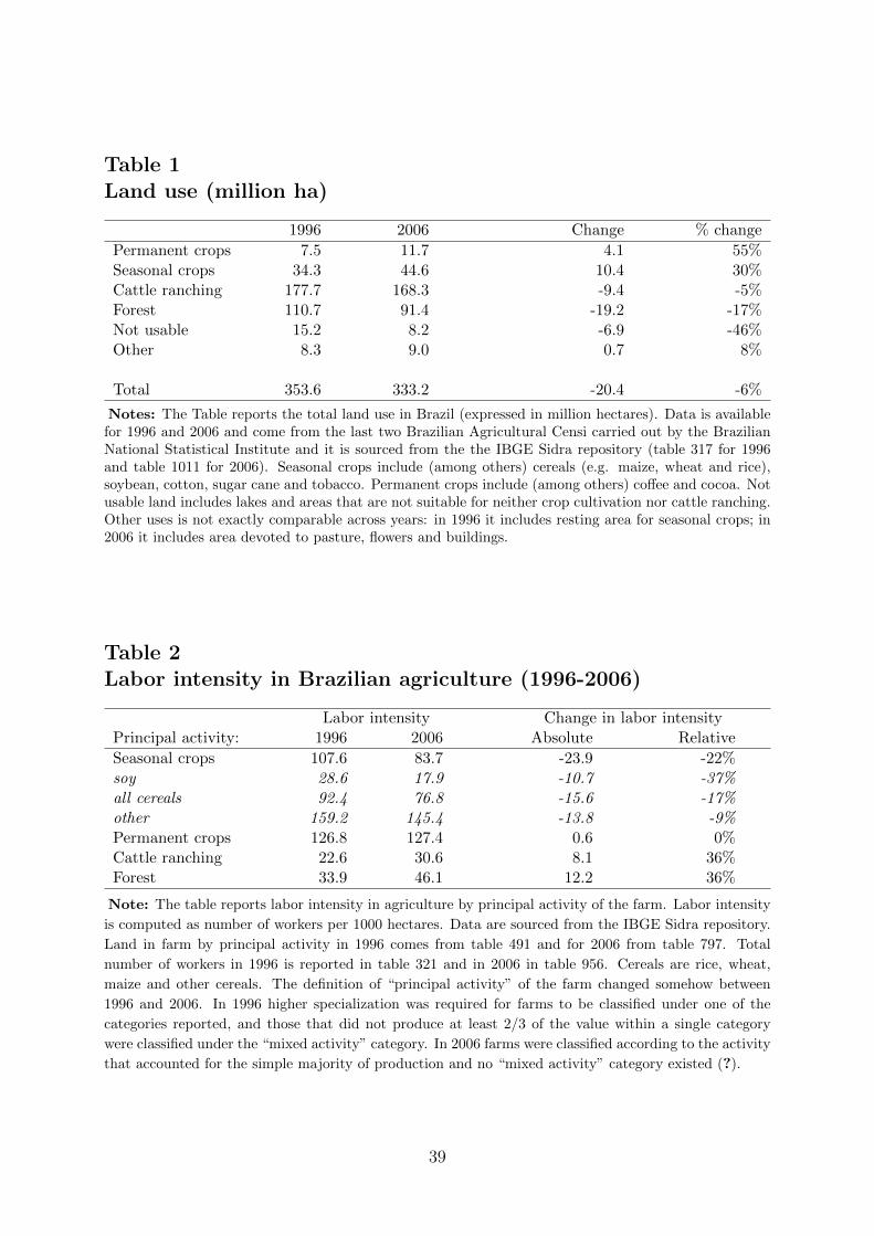
Table 1Land use (million ha)

1996 2006 Change % change

Permanent crops 7.5 11.7 4.1 55%Seasonal crops 34.3 44.6 10.4 30%Cattle ranching 177.7 168.3 -9.4 -5%Forest 110.7 91.4 -19.2 -17%Not usable 15.2 8.2 -6.9 -46%Other 8.3 9.0 0.7 8%

Total 353.6 333.2 -20.4 -6%

Notes: The Table reports the total land use in Brazil (expressed in million hectares). Data is availablefor 1996 and 2006 and come from the last two Brazilian Agricultural Censi carried out by the BrazilianNational Statistical Institute and it is sourced from the the IBGE Sidra repository (table 317 for 1996and table 1011 for 2006). Seasonal crops include (among others) cereals (e.g. maize, wheat and rice),soybean, cotton, sugar cane and tobacco. Permanent crops include (among others) coffee and cocoa. Notusable land includes lakes and areas that are not suitable for neither crop cultivation nor cattle ranching.Other uses is not exactly comparable across years: in 1996 it includes resting area for seasonal crops; in2006 it includes area devoted to pasture, flowers and buildings.

Table 2Labor intensity in Brazilian agriculture (1996-2006)

Labor intensity Change in labor intensityPrincipal activity: 1996 2006 Absolute Relative

Seasonal crops 107.6 83.7 -23.9 -22%soy 28.6 17.9 -10.7 -37%all cereals 92.4 76.8 -15.6 -17%other 159.2 145.4 -13.8 -9%Permanent crops 126.8 127.4 0.6 0%Cattle ranching 22.6 30.6 8.1 36%Forest 33.9 46.1 12.2 36%

Note: The table reports labor intensity in agriculture by principal activity of the farm. Labor intensity

is computed as number of workers per 1000 hectares. Data are sourced from the IBGE Sidra repository.

Land in farm by principal activity in 1996 comes from table 491 and for 2006 from table 797. Total

number of workers in 1996 is reported in table 321 and in 2006 in table 956. Cereals are rice, wheat,

maize and other cereals. The definition of “principal activity” of the farm changed somehow between

1996 and 2006. In 1996 higher specialization was required for farms to be classified under one of the

categories reported, and those that did not produce at least 2/3 of the value within a single category

were classified under the “mixed activity” category. In 2006 farms were classified according to the activity

that accounted for the simple majority of production and no “mixed activity” category existed (?).

39

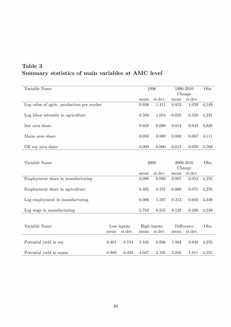
Table 3Summary statistics of main variables at AMC level

Variable Name 1996 1996-2010 Obs.Change

mean st.dev. mean st.dev.

Log value of agric. production per worker 0.938 1.411 0.853 1.059 4,149

Log labor intensity in agriculture -2.594 1.054 -0.025 0.556 4,231

Soy area share 0.028 0.099 0.012 0.043 3,920

Maize area share 0.050 0.069 0.008 0.067 4,111

GE soy area share 0.000 0.000 0.013 0.059 3,769

Variable Name 2000 2000-2010 Obs.Change

mean st.dev. mean st.dev.

Employment share in manufacturing 0.098 0.086 0.007 0.052 4,255

Employment share in agriculture 0.405 0.197 -0.066 0.075 4,255

Log employment in manufacturing 6.006 1.597 0.213 0.603 4,249

Log wage in manufacturing 5.753 0.555 0.128 0.426 4,249

Variable Name Low inputs High inputs Difference Obs.mean st.dev. mean st.dev. mean st.dev.

Potential yield in soy 0.301 0.154 2.105 0.936 1.804 0.849 4,255

Potential yield in maize 0.989 0.493 4.047 2.195 3.058 1.811 4,255

40

Table 4Basic correlations in the data: agricultureProductivity, labor intensity and employment share

(1) (2) (3)VARIABLES ∆ Value per worker ∆ Labor intensity ∆ Employment share

∆ Soy area share 2.350*** -0.484*** -0.058**(0.297) (0.154) (0.027)

∆ Maize area share 2.410*** 0.746*** -0.024(0.229) (0.119) (0.019)

Constant 0.120*** -0.029*** -0.066***(0.018) (0.009) (0.001)

Observations 3,753 3,805 3,805

Note: The table reports the OLS estimated coefficients of equation 8 in the text. The independent

variables are defined as the share of farm land reaped with soy and maize. The dependent variables are

reported on top of the respective columns. Value per worker is defined as total value of output in farms

whose main activity is seasonal crop cultivation divided by the total number of workers employed by

these farms. Labor intensity is the total number of workers employed in agriculture divided by total area

in farms. Share of workers employed in agriculture is defined as total number of workers in agriculture

divided by total number of workers in all sectors. The source of data for the independent variables and

the dependent variables reported in columns 1 and 2 are the agricultural censi of 1996 and 2006. Thus,

changes are calculated over the years 1996 and 2006. The source for the employment share reported in

column 3 are the population censi of 2000 and 2010. In this case, changes in the dependent variable are

calculated over the years 2000 and 2010. The unit of observation are municipalities. Robust standard

errors are reported in parentheses. Significance levels: *** p<0.01, ** p<0.05, * p<0.1.

41

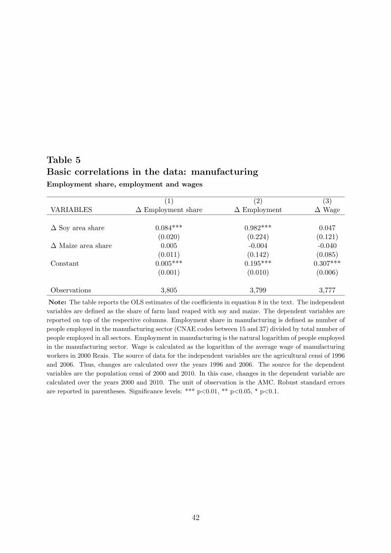
Table 5Basic correlations in the data: manufacturingEmployment share, employment and wages

(1) (2) (3)VARIABLES ∆ Employment share ∆ Employment ∆ Wage

∆ Soy area share 0.084*** 0.982*** 0.047(0.020) (0.224) (0.121)

∆ Maize area share 0.005 -0.004 -0.040(0.011) (0.142) (0.085)

Constant 0.005*** 0.195*** 0.307***(0.001) (0.010) (0.006)

Observations 3,805 3,799 3,777

Note: The table reports the OLS estimates of the coefficients in equation 8 in the text. The independent

variables are defined as the share of farm land reaped with soy and maize. The dependent variables are

reported on top of the respective columns. Employment share in manufacturing is defined as number of

people employed in the manufacturing sector (CNAE codes between 15 and 37) divided by total number of

people employed in all sectors. Employment in manufacturing is the natural logarithm of people employed

in the manufacturing sector. Wage is calculated as the logarithm of the average wage of manufacturing

workers in 2000 Reais. The source of data for the independent variables are the agricultural censi of 1996

and 2006. Thus, changes are calculated over the years 1996 and 2006. The source for the dependent

variables are the population censi of 2000 and 2010. In this case, changes in the dependent variable are

calculated over the years 2000 and 2010. The unit of observation is the AMC. Robust standard errors

are reported in parentheses. Significance levels: *** p<0.01, ** p<0.05, * p<0.1.

42

Table 6The effect of technological change on agricultureSoy and maize expansion

(1) (2) (3) (4)VARIABLES ∆ Soy area share ∆ Maize area share

∆Asoy 0.012*** 0.014*** -0.006***(0.001) (0.002) (0.002)

∆Amaize -0.002** 0.003*** 0.005***(0.001) (0.001) (0.001)

Constant -0.009*** -0.009*** -0.000 0.004(0.001) (0.001) (0.002) (0.002)

Observations 3,920 3,920 4,111 4,111

Note: The table reports the OLS estimates of the coefficients in equation 11 in the text. Dependent

variables – reported on top of the respective columns – are defined as the share of farm land reaped with

soy and maize. ∆Asoy is defined as potential soy yield under high inputs minus potential soy yield under

low inputs. ∆Amaize is defined as potential maize yield under high inputs minus potential maize yield

under low inputs. The source of data for the dependent variables are the agricultural censi of 1996 and

2006. Thus, changes are calculated over the years 1996 and 2006. The source of data for the independent

variables is the FAO-GAEZ v3.0 dataset. The unit of observation is the AMC. Robust standard errors

are reported in parentheses. *** p<0.01, ** p<0.05, * p<0.1.

Table 7The effect of technological change on agricultureGE soy adoption

(1) (2)VARIABLES ∆ GE soy area share ∆ Non-GE soy area share

∆Asoy 0.017*** -0.007***(0.002) (0.002)

Constant -0.017*** 0.011***(0.002) (0.002)

Observations 3,769 3,769

Note: The table reports the OLS estimates of the coefficients in equation 11 in the text where the

dependent variable is defined as the share of farm land reaped with GE soy (column 1) and non-GE soy

(column 2). ∆Asoy is defined as potential soy yield under high inputs minus potential soy yield under

low inputs. The source of data for the independent variables are the agricultural censi of 1996 and 2006.

Thus, changes are calculated over the years 1996 and 2006. The source of data for the independent

variables is the FAO-GAEZ v3.0 dataset. The unit of observation is the AMC. Robust standard errors

in parentheses. *** p<0.01, ** p<0.05, * p<0.1.

43

Table 8The effect of technological change on agricultureProductivity, labor intensity and employment share

(1) (2) (3)VARIABLES ∆ Value per worker ∆ Labor intensity ∆ Employment share

∆Asoy 0.090*** -0.034** 0.000(0.031) (0.016) (0.002)

∆Amaize -0.017 0.024*** -0.001(0.015) (0.008) (0.001)

Constant 0.045 -0.037* -0.063***(0.037) (0.019) (0.003)

Observations 4,149 4,231 4,255

Note: The table reports the OLS estimates of the coefficients in equation 11 in the text. The dependent

variables are reported on top of the respective columns. Value per worker is defined as total value of

output in farms whose main activity is seasonal crop cultivation divided by the total number of workers

employed by these farms. Labor intensity is the total number of workers employed in agriculture divided

by total area in farms. Share of workers employed in agriculture is defined as total number of workers

in agriculture divided by total number of workers in all sectors. ∆Asoy is defined as potential soy yield

under high inputs minus potential soy yield under low inputs. ∆Amaize is defined as potential maize yield

under high inputs minus potential maize yield under low inputs. The source of data for the dependent

variables reported in columns 1 and 2 are the agricultural censi of 1996 and 2006. Thus, changes are

calculated over the years 1996 and 2006. The source for the employment share reported in column 3 are

the population censi of 2000 and 2010. In this case, changes in the dependent variable are calculated

over the years 2000 and 2010. The source of data for the independent variables is the FAO-GAEZ v3.0

dataset. The unit of observation is the AMC. Robust standard errors are reported in parentheses. ***

p<0.01, ** p<0.05, * p<0.1.

44

Table 9The effect of technological change on manufacturingEmployment share, employment and wages

(1) (2) (3)VARIABLES ∆ Employment share ∆ Employment ∆ Wage

∆Asoy 0.018*** 0.241*** -0.071***(0.002) (0.016) (0.012)

∆Amaize -0.003*** -0.062*** 0.030***(0.001) (0.008) (0.005)

Constant -0.015*** -0.032 0.339***(0.002) (0.021) (0.014)

Observations 4,255 4,249 4,226

Note: The table reports the OLS estimates of the coefficients in equation 11 in the text. The dependent

variables are reported on top of the respective columns. Employment share in manufacturing is defined

as number of people employed in the manufacturing sector (CNAE codes between 15 and 37) divided by

total number of people employed in all sectors. Employment in manufacturing is the natural logarithm

of people employed in the manufacturing sector. Wage is calculated as the logarithm of the average wage

of manufacturing workers in 2000 Reais. ∆Asoy is defined as potential soy yield under high inputs minus

potential soy yield under low inputs. ∆Amaize is defined as potential maize yield under high inputs minus

potential maize yield under low inputs. The source for the dependent variables are the population censi

of 2000 and 2010. In this case, changes in the dependent variable are calculated over the years 2000

and 2010. The source of data for the independent variables is the FAO-GAEZ v3.0 dataset.The unit of

observation is the AMC. Robust standard errors are reported in parentheses. Significance levels: ***

p<0.01, ** p<0.05, * p<0.1.

45

Table 10Basic correlations in the data: manufacturingEmployment share, employment and wages

Robustness of results reported in Table 5 to a larger unit of observation: micro-

regions

(1) (2) (3)VARIABLES ∆ Employment share ∆ Employment ∆ Wage

∆ Soy area share 0.093* 0.906** 0.043(0.049) (0.396) (0.228)

∆ Maize area share 0.038 0.126 0.259(0.032) (0.468) (0.207)

Constant -0.003** 0.170*** 0.262***(0.001) (0.015) (0.009)

Observations 557 557 556

Note: The table reports the OLS estimates of the coefficients in equation 8 in the text. The independent

variables are defined as the share of farm land reaped with soy and maize. The dependent variables are

reported on top of the respective columns. Employment share in manufacturing is defined as number of

people employed in the manufacturing sector (CNAE codes between 15 and 37) divided by total number of

people employed in all sectors. Employment in manufacturing is the natural logarithm of people employed

in the manufacturing sector. Wage is calculated as the logarithm of the average wage of manufacturing

workers in 2000 Reais. The source of data for the independent variables are the agricultural censi of 1996

and 2006. Thus, changes are calculated over the years 1996 and 2006. The source for the dependent

variables are the population censi of 2000 and 2010. In this case, changes in the dependent variable are

calculated over the years 2000 and 2010. The unit of observation is the micro-region. Robust standard

errors are reported in parentheses. Significance levels: *** p<0.01, ** p<0.05, * p<0.1.

46

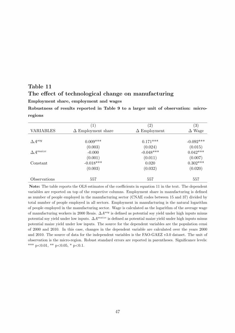
Table 11The effect of technological change on manufacturingEmployment share, employment and wages

Robustness of results reported in Table 9 to a larger unit of observation: micro-

regions

(1) (2) (3)VARIABLES ∆ Employment share ∆ Employment ∆ Wage

∆Asoy 0.009*** 0.171*** -0.092***(0.003) (0.024) (0.015)

∆Amaize -0.000 -0.048*** 0.042***(0.001) (0.011) (0.007)

Constant -0.018*** 0.020 0.302***(0.003) (0.032) (0.020)

Observations 557 557 557

Note: The table reports the OLS estimates of the coefficients in equation 11 in the text. The dependent

variables are reported on top of the respective columns. Employment share in manufacturing is defined

as number of people employed in the manufacturing sector (CNAE codes between 15 and 37) divided by

total number of people employed in all sectors. Employment in manufacturing is the natural logarithm

of people employed in the manufacturing sector. Wage is calculated as the logarithm of the average wage

of manufacturing workers in 2000 Reais. ∆Asoy is defined as potential soy yield under high inputs minus

potential soy yield under low inputs. ∆Amaize is defined as potential maize yield under high inputs minus

potential maize yield under low inputs. The source for the dependent variables are the population censi

of 2000 and 2010. In this case, changes in the dependent variable are calculated over the years 2000

and 2010. The source of data for the independent variables is the FAO-GAEZ v3.0 dataset. The unit of

observation is the micro-region. Robust standard errors are reported in parentheses. Significance levels:

*** p<0.01, ** p<0.05, * p<0.1.

47

Table 12The effect of technological change on manufacturingEmployment and wages

Falsification test of results reported in Table 9: checking for pre-existing trends

(1) (2)VARIABLES ∆ Employment ∆ Wage

∆Asoy -0.019 -0.001(0.020) (0.026)

∆Amaize 0.001 0.020*(0.009) (0.012)

Constant 0.246*** -0.157***(0.025) (0.033)

Observations 4,231 4,096

Note: The table reports the OLS estimates of the coefficients in equation 11 in the text. The dependent

variables are reported on top of the respective columns. Employment in manufacturing is the natural

logarithm of people employed in the manufacturing sector. Wage is calculated as the logarithm of the

average wage of manufacturing workers in 2000 Reais. ∆Asoy is defined as potential soy yield under high

inputs minus potential soy yield under low inputs. ∆Amaize is defined as potential maize yield under

high inputs minus potential maize yield under low inputs. The source for the dependent variables are the

population censi of 1991 and 2000. In this case, changes in the dependent variable are calculated over the

years 1991 and 2000. The source of data for the independent variables is the FAO-GAEZ v3.0 dataset.

The unit of observation is the AMC. Robust standard errors are reported in parentheses. Significance

levels: *** p<0.01, ** p<0.05, * p<0.1.

48

Table 13The effect of technological change on manufacturingEmployment and wages

Robustness of results reported in Table 9 to controlling for commodity prices

(1) (2) (3) (4)VARIABLES Total Employment Total Employment Wage Wage

Asoy 0.073** 0.077*** -0.046*** -0.040***(0.029) (0.028) (0.014) (0.014)

Amaize -0.013 -0.016 0.020*** 0.019***(0.015) (0.015) (0.007) (0.007)

P zAz controls No Yes No Yes

AMC & year FE Yes Yes Yes Yes

Observations 20,740 20,740 20,718 20,718

Note: The table reports the OLS estimates of the coefficients in equation 12 in the text. The dependent

variables are reported on top of the respective columns. Total employment is the natural logarithm of the

total number of workers employed in manufacturing plants (CNAE 1.0 codes 15 to 37) owned by firms

that employ at least 30 employees within an AMC. The average wage is computed from manufacturing

plants (CNAE 1.0 codes 15 to 37) owned by firms that employ at least 30 employees. Wage is defined as

the aggregate wage bill (in real terms) across firm within an AMC divided by total number of workers

across the same firms within the same AMC. Asoy is defined as potential soy yield under high inputs for

the years between 2003 and 2006, and the potential soy yield under low inputs for the years between 1996

and 2002. Amaize is defined as potential maize yield under high inputs for the years between 2003 and

2006, and potential maize yield under low inputs for the years between 1996 and 2002. P zAz controls

stand for the interaction of the potential yield of soy and maize under low inputs interacted with price

levels of these crops between 1996 and 2006. The source for the dependent variables is the plant-level

supplement of the yearly industrial survey (PIA) for the years 1996 to 2006. The source of data for the

independent variables is the FAO-GAEZ v3.0 dataset. The unit of observation is the AMC. Standard

errors clustered at AMC level are reported in parentheses. Significance levels: *** p<0.01, ** p<0.05, *

p<0.1.

49