Agricultural Trade, Institutions, and Depletion of Natural Resources∗

Sheetal Sekhri,† Paul Landefeld‡

This Draft: September 2013

Abstract

Globalization can lead to either conservation or depletion of natural resources that are

used in the production of traded goods. Rising prices may lead to better resource man-

agement. Alternatively, stronger incentives to extract these resources may exacerbate

their decline- especially in open access institutional frameworks. We examine the impact

of agricultural trade promotion on the groundwater extraction in India using nationally

representative data from 1996-2005. We find evidence that trade promotion leads to de-

pletion of groundwater reserves. Access to world markets does not result in emergence of

institutions that would enable protection of the resource.

JEL classification: O13, Q25, Q56

Keywords: Groundwater Depletion, Agricultural Trade

∗We thank Central Groundwater Board of India for providing the groundwater data. The paper benefitted

from comments by Andrew Foster, Leora Friedberg, James Harrigan, Amit Khandelwal, John Mclaren, Ariell

Reshef, and Sriniketh Nagavarapu. Sekhri thanks the Sustainability Science Program at the Kennedy School

of Government for its support and hospitality. Sekhri also thankfully acknowledges funding from the Bankard

Fund for Political Economy. This paper represents the views of the authors alone. It should not be construed

as representing the views or policies of the staff of the Joint Committee on Taxation or any member of the

United States Congress.

†University of Virginia, PO Box 400182, Department of Economics, Monroe Hall, Charlottesville, VA 22904-

4182 Email: SSekhri@virginia.edu

‡Joint Committee on Taxation Email: paul.landefeld@jct.gov

1 Introduction

Promoting the trade of goods that use natural resources as factors of production can have

consequences for these resources. However, the nature of these consequences is not well es-

tablished. Prominent theories investigating the linkage between trade and natural resources

indicate that access to world markets may generate strong incentives to improve resource

management (Copeland and Taylor, 2009). Non-market institutions that promote resource

conservation may emerge (Ostrom, 1990; Ostrom, 2010).1 On the other hand, trade pro-

motion in economies with an open-access property rights regime may exacerbate extraction.

These competing effects make the impact of trade promotion on resource stocks theoreti-

cally unclear. Rigorous empirical examination of this relationship is especially important in

poor and predominantly agricultural economies that use agricultural trade promotion as a

policy lever to improve standards of living. In this paper, we explore whether promotion of

agricultural trade leads to conservation of groundwater.

Groundwater is mined for irrigation use in many industrialized and developing countries

including India, Pakistan, China, Yemen, and the United States. Access to this resource

can lead to manifold increases in agricultural productivity but also raises the risk of its

depletion. Declining water tables can threaten food security and compromise the ability to

mitigate droughts.2 Groundwater is also used to meet drinking water needs in many parts

of the world. Concerns about changing precipitation patterns due to global warming have

made sustaining groundwater reserves even more critical. Thus, from a policy perspective,

understanding how groundwater can be used in a sustainable manner is vital.

We explore the introduction of agricultural trade promotion zones in India to make two

contributions to the literature. First, our study identifies the causal impact of an increase in

international trade on renewable resources in an economy with open-access property rights.

We present novel evidence on the impact of agricultural trade promotion on groundwater

resources used as a factor of production in agriculture. Second, we estimate reduced-form

welfare gains by examining changes in per-capita expenditure and rural wages. To carry out

our empirical analysis, we collated a unique dataset that includes nationally representative

groundwater data from 1996 to 2005 covering 16,000 observation wells in the country.

1In her influential work on the emergence of non-market institutions to promote conservation of open-access

resources, Ostrom has provided many case studies highlighting when and where these institutions emerge.2Water table is the depth below surface of earth where water is first encountered at atmospheric pressure.

2

India is a pertinent setting in which to explore the relationship between agricultural trade

promotion and depletion of groundwater for a number of reasons. India extracts the largest

amount of groundwater in the world, almost twice as much as the United States. Around

60 percent of Indian agriculture is sustained by groundwater. Between 1980 and 2010, water

tables declined by more than 12 meters in many parts of India, and the depletion rates

have been accelerating since 2000 (Rodell at al., 2009; Sekhri, 2012). According to the

satellite-data-based study conducted by NASA, the rate at which aquifers are being mined in

India is unsustainable (Rodell at al., 2009). Sekhri (2013 a) finds that a 1 meter decline in

district water tables below its long-term mean in India reduces production of food grains by

8 percent. Groundwater scarcity increases rural poverty by almost 12 percent (Sekhri, 2013

b). According to an estimate of the International Water Management Institute, the current

patterns of extraction in India could lead to a 25 percent decline in food production by 2025

(Seckler et al, 1998). Given that malnutrition, especially among children, is high in India,3

conserving groundwater and ensuring food security are first-order policy goals.

The Government of India introduced Agricultural Export Promotion Zones (AEZs) in its

exim (export-import) policy of 2001. These AEZs provide integrated services such as pack-

aging, agricultural extension, quality control, and upgrading to geographically concentrated

clusters of administrative jurisdictions (districts) to promote export of government-approved

cash crops. We use geographical neighbors of the AEZs as the counterfactual in our empirical

analysis. The major determinant of selection was suitability for the approved cash crop, which

is affected by characteristics of districts that do not change in the short-run, such as geology

and geography. The inclusion of district fixed effects in our regression analysis accounts for

differences in suitability for various crops. We also control for AEZ cluster fixed effects, so

that the identification comes from the comparison of districts specific to an AEZ cluster to

their neighbors over time. Shared geographical neighbors across different clusters and multi-

ple AEZs in districts allow us to control for these two sets of fixed effects.4 Our long panel

3Almost 40 percent of the world’s malnourished children live in India (Von Braun et al., 2008).4 We do not compare the set of districts that received an AEZ to the set of districts that comprise geograph-

ical neighbors of these districts. The control set in such a comparison may not be in proximity to the treated

districts and thus may be less comparable in crop suitability. Rather, we compare districts in a specific AEZ

to its geographical neighbors. To identify the effect of million-dollar plants on local economies, Greenstone

et al. (2010) make this type of dyadic comparison between counties that win such plants and those that lose

them.

3

data allow us to establish that pre-policy trends in groundwater depth do not confound our

results. Our identifying assumption is that conditional on district fixed effects and these pre-

trends, the neighboring districts form valid counterfactuals for the treated districts. We show

that prior to AEZ establishment, treated districts have similar trends in most economic and

demographic variables compared to the neighboring districts. We do not rely on early versus

late adoption of AEZ for identification because the timing may be influenced by financial

constraints, and hence may be endogenous. Although our results are larger in specifications

comparing early to late adopters, we illustrate that the timing of adoption is correlated with

trends in economic variables.

We find that the introduction of AEZs leads to an increase in exports but depletes the

groundwater resource more rapidly. Following Brander and Taylor (1997) and Taylor (2011),

we conjecture that the underlying mechanism is entry of more farmers into growing cash crops.

Using Taylor’s framework, we illustrate that such entry can lead to depletion of groundwater.

To corroborate our study design, we conduct a placebo test to show that AEZ clusters that

were planned but not implemented did not experience any changes in depth to groundwater.

To examine spill-overs, we carry out our analysis on a restricted sample of districts that

are on the geographical boundaries of the clusters. Our results in this restricted sample are

similar to those in the full sample, indicating the absence of spatial spill-over effects. Finally,

we estimate reduced-form effects on mean per-capita expenditure (mpce) and rural wages.

Mean per-capita expenditure is higher and significant for landowners relative to the landless.

Consistently, we do not detect any effect on rural wages. Among cultivating farmers, the

effect on mpce does not vary by holding size. Small and large farmers benefit from the AEZ.

For the farmers with median land-holdings, 72 percent of the change in mpce is attributable

to the change in groundwater depth. Our estimates imply that a decline of 0.4 meters in

groundwater depth results in an increase of 91 rupees (0.17 of a within-district standard

deviation) in per-capita expenditure for the median farming household. At the shadow price

equivalent to the price of metered water delivered to households, this gain in mpce would be

much lower than the social cost of groundwater.

This paper contributes to the literature on trade promotion and depletion of natural re-

sources. Current theoretical insights offer mixed findings depending on how increased exports

alter the trajectory of prices. Copeland and Taylor (2009) develop a model that lays out the

conditions under which trade can lead to conservation of renewable resources. They argue

4

that an increase in the price of the product resulting from favorable terms of trade may lead

to the emergence of institutions that help conserve natural resources. Property rights that

promote conservation can emerge as a result of increased trade. Foster and Rosenzweig (2003)

present empirical evidence to demonstrate that increased prices for forest products between

1977 and 1999 in India, albeit resulting from increase in local demand for forest goods, led

to a revival of the forests and decelerated deforestation. Kremer and Morcom (2000) develop

a model in which open-access resources are used for production of storable goods, and show

that both survival and extinction equilibria are likely to arise. Chichilnisky (1994) and Bran-

der and Taylor (1997) present theoretical arguments; Taylor (2011) and Lopez (1997, 1998)

develop theories and offer supporting evidence from the historical extinction of buffalo in US

and African agriculture respectively.5 However, lack of available data has contributed to the

paucity of careful causal analysis on how trade in goods using renewable resources influences

the stock of those resources due to the evolution or lack thereof of pertinent institutions.

Another pressing empirical problem for such analysis is that the availability or abundance of

the renewable resource might influence policies that promote trade making the identification

of causal effects difficult. Our comprehensive data and study design allow us to circumvent

these issues. To the best of our knowledge, our study is the first to present evidence on the

effects of agricultural trade promotion on groundwater.

The rest of the paper is organized as follows: Section 2 provides background on AEZs in

India and their selection process. Section 3 discusses the data we use in our empirical work.

Section 4 presents our estimation Strategy. Section 5 discusses the main results. Section

6 explains the mechanism relying on a model of entry into cash crops. Section 7 presents

results from robustness tests and evidence in support of our theory. Section 8 presents the

reduced-form effects on mean per-capita expenditure and rural wages. Section 9 provides

concluding remarks.

2 Background

2.1 Agricultural Export Promotion Zones

The government of India created the concept of AEZ under its exim Policy of 2001 to promote

the export of cash crops. It nominated the Agricultural and Processed Food Products Export

5Bulte and Barbier (2005) review the literature on trade and property rights.

5

Development Authority (APEDA) as the nodal agency to oversee the creation and operations

of these zones. In establishing an AEZ, the government designates a potential product for

export and a contiguous geographical region in which this product can be grown. Subse-

quently, production, packaging, and transportation of APEDA-approved cash crops, which

have a high return on investment, are integrated within the zone. The government provides

financial assistance for training and extension services, research and development, quality up-

grading, and marketing. At the time of establishment, the government anticipated that these

zones would increase value addition, improve quality, increase competitiveness, bring down

the cost of production due to economies of scale, increase research and development for trade

promotion, and increase employment. Individual states nominated clusters, comprising either

a single district or a block of districts, and products for centralized approval. Each cluster was

envisioned to have research and development support from a nearby agricultural university.

States are also expected to provide institutional support for smooth day-to-day functioning

of the zone. Importantly, pricing or provision of electricity did not change due to setting

up of an AEZ.6 As of 2008, 60 AEZ clusters had been created. 7 In our empirical analysis,

we use 42 out of the 60 AEZs; we dropped nine clusters because the AEZ was never made

operational, and another nine due to a lack of groundwater data for the districts involved.

We use the planned but not operationalized AEZs to conduct a falsification test and validate

that an increase in exports of cash crops due to AEZ establishment drives our results.

2.2 Selection of Agricultural Export Zones

The states had to choose feasible cash crops and clusters of areas that could grow these

cash crops. Thus, an important criterion in selecting the AEZ cluster sites was suitability

for growing the cash crops. Suitability for growing crops in a geographical area is largely

6Many states in India already subsidize electricity for agriculture; thus the marginal cost of extraction is

negligible. No concurrent changes in agricultural electricity pricing occurred that can drive the results. For

example, Punjab (a major agricultural state experiencing significant declines in groundwater) went from flat

tariffs for agricultural electricity usage to free provision in 1997. The free provision was reversed in 2002 and

then instituted again in 2005. Relative to the previous decade, groundwater depth in Punjab did not drop

significantly after 1997, but rather after 2001, when two AEZs had been established. Furthermore, the depleting

trend did not reverse between 2002 and 2005, when free provision was reversed. In addition, electricity pricing

would have to change differentially for a districts receiving AEZs and neighbors within a state to drive the

results. But within-state pricing policies are uniformly applied to all districts.7 Districts in our sample can be a part of more than one AEZ cluster established at different times.

6

determined by static factors such as soil characteristics, long term climate, and geographical

characteristics such as elevation and slope. Support from an agricultural university was

also deemed important and proximity to such universities influenced the selection of cluster

locations.

States also had to provide substantial financial support for the AEZs. Appendix Table 1

shows the details of government expenditures, the product for which AEZ was launched, the

state and districts of establishment, and the date of approval and commencement. Suitability

influenced the location, whereas institutional and financial constraints of the states influenced

the timing of creation. Appendix Figure 1 shows the distribution of the dates of establishment

of these zones. Among the AEZs established by 2008, the median number were established

by December, 2002. Becasue the timing was largely governed by financial and institutional

constraints, we do not rely on timing of implementation for identification. We provide more

details in section 7.4.

To address endogeneity concerns, we use neighboring districts that did not receive an AEZ

as counterfactuals. We compare the groundwater depths for these districts before and after

the AEZ creation using a long panel of groundwater data. Our identifying assumption is that

neighboring districts provide a good counterfactual in terms of potential to grow the cash

crops. The geographical neighbors we use as controls are comparable in crop suitability to

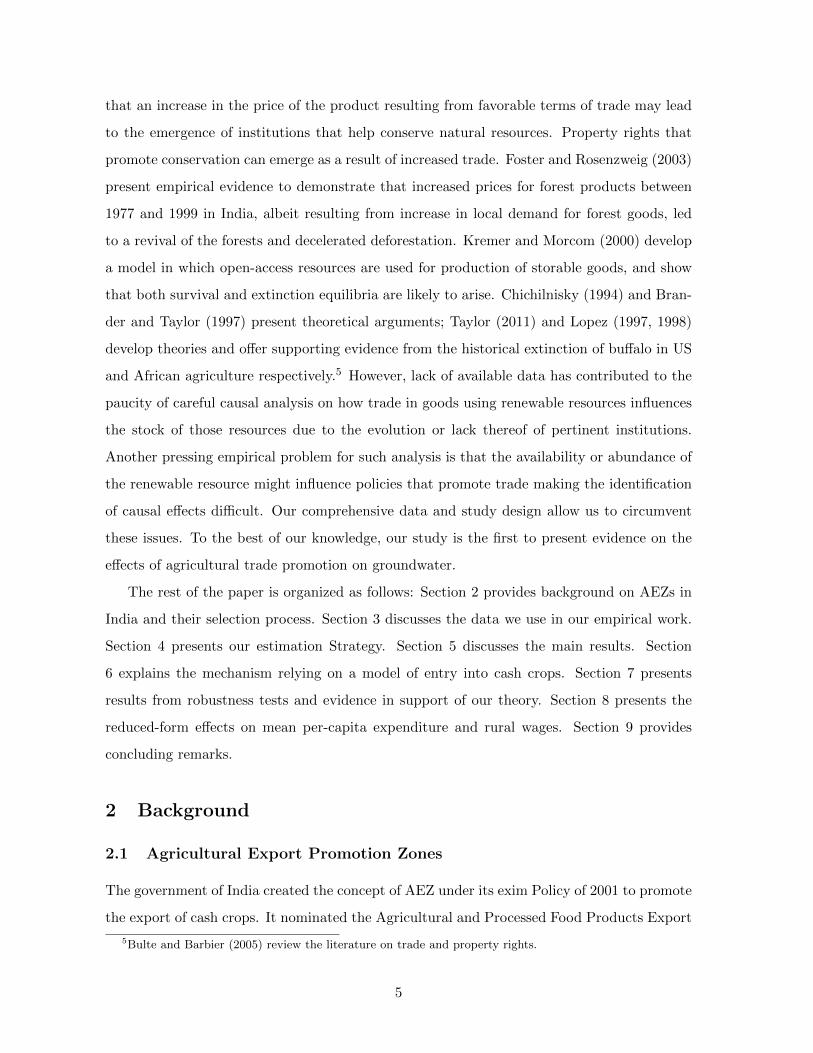
the treated districts and are in close proximity to agricultural universities. Figure 1 maps the

districts that were in an AEZ by 2008 along with their neighbors and locations of agricul-

tural universities to highlight that the agricultural universities were equidistant.8 We discuss

selection into treatment and its implications in detail in section 4.2.

3 Data

The groundwater data comes from individual monitoring wells of the Indian Central Ground

Water Board. These data are collected from around 16,000 monitoring or observation wells

that are spread through out the country. Groundwater measurements are taken four times

a year at these monitoring wells, once in each quarter – in May/June, August, November,

8We do not have data for some of the geographical neighbors. In addition, some universities were established

after 2001 by the time the exim policy had been already announced. Appendix Figure 2 maps the districts

that were in an AEZ and indicates neighbors for which we do not have data. This map also indicates the

locations of universities by the establishment date.

7

and January. These well data have been aggregated spatially to the district level using the

spatial boundaries of Indian districts corresponding to the 2001 Census of India. We use both

quarterly and annual average district -level data in the empirical analysis.

Precipitation and temperature data from the University of Delaware Center for Climactic

Research are used to calculate district annual average monthly precipitation and tempera-

ture. The Center for Climactic Research at the University of Delaware compiled monthly

weather station data from 1900 to 2008 from several sources.9 After combining data from

various sources, the Center for Climactic Research used various spatial interpolation and

cross-validation methods to construct a global 0.5 degree by 0.5 degree latitude/longitude grid

of monthly precipitation and temperature data from 1900 to 2008 (Matsuura and Wilmott,

2009). From these data, all grid points within India’s administrative boundaries were ex-

tracted to construct district-level annual average and monthly precipitation and temperature

in each year. In addition, we take district demographic and socioeconomic characteristics

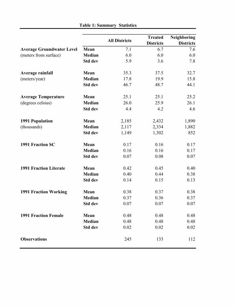
from the 2001 Census of India. Table 1 reports the summary statistics. Our sample contains

245 districts, of which 133 districts received an AEZ and 112 constitute neighboring controls.

Table 1 reports the summary statistics. Overall average depth to groundwater in the

sample is 7.1 meters below ground level (mbgl). The average is 6.7 mbgl for the treated

districts and 7.6 mbgl for the control districts. The sample median is 6 mbgl. The overall

standard deviation is 5.9 mbgl. The standard deviation in the treated group is smaller at 3.6

than the control group at 7.8 mbgl. The average annual rainfall is 35.4 mm per annum. The

treated areas on average receive more rainfall but the variability in rainfall is also higher. The

average annual temperature is 25.1 degree centrigrade and is comparable across the treated

and control areas. The treated areas are more populous as per the Census of India 1991. In

the sample, 38 percent of the population is employed in 1991. Around 48 percent is female

and 17 percent is scheduled castes.10 These characteristics are very similar across treated

and control group districts. Average Literacy rate is 42 percent. In levels, the treated areas

have higher literacy in 1991. But we later show that these variables do not exhibit differential

9 These sources include the Global Historical Climatology Network, the Atmospheric Environment Ser-

vice/Environment Canada, the Hydrometeorological Institute in St. Petersburg, Russia, GC-Net, the Auto-

matic Weather Station Project, the National Center for Atmospheric Research, Sharon Nicholson’s archive

of African precipitation data, Webber and Willmott’s (1998) South American monthly precipitation station

records, and the Global Surface Summary of Day.10Scheduled Castes are historically marginalized population group in India.

8

trends.

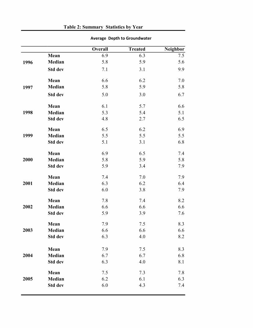
Table 2 shows the summary statistics for the depth to groundwater by year. In 1996, the

average depth was 6.9 mbgl, whereas in 2001, the average depth was 7.4 mbgl. This further

fell to 7.9 mbgl in 2002. The average depth to groundwater in treated districts was 6.3 mbgl

in 1996, whereas it was 7.5 in the control areas. The variability in depth is also lower in

the treated areas. Overall depth to groundwater in both the treated and control areas was

declining over this time period. In the treated areas, depth to groundwater fell by 1 meter

and in control areas, it fell by only 0.3 meters. Prior to treatment, the treated areas had

shallower water tables. In what follows, we show that much of this rapid decline in treated

areas resulted from promotion of AEZs.

4 Estimation Strategy

4.1 Empirical Model

The main empirical challenge in estimating the effects of the establishment of AEZs on ground-

water decline is that districts for AEZs were not randomly chosen. As mentioned before, in

order to address endogeneity concerns, we use neighboring districts that did not receive an

AEZ as counterfactuals. We compare the groundwater depths for AEZ districts and neighbors

before and after the AEZ’s establishment, using a long panel of groundwater data.11

The empirical model is as follows:

Wdt = α0 +Ac +Dd +Qt + trendt + α1 Post ∗ T + α2 Xdt + εdt (1)

where Wdt is the depth to groundwater in district d at time t. Post is an indicator that

takes value 1 after an AEZ has been established in a district and 0 before. T is an indicator

that takes the value 1 if a district is a part of the AEZ cluster. Qt is an indicator for the

quarter of the year in which groundwater measurement is taken to account for the seasonality

in depth of groundwater. trendt is a linear time trend and controls for any secular changes

in depth over time. Xdt are time-varying characteristics of the districts that may vary across

11We do not have district specific data on production of all APEDA-approved crops. Hence, we do not

estimate a 2SLS model in which the first stage would show the effect of the policy shift on area under cultivation

of cash crops and the second stage would show how increased area under cultivation shifts water tables.

9

treatment and control districts and influence selection into treatment. εdt is the standard

error. Robust standard errors are clustered by district.

In addition, we control for two sets of fixed effects. Ac are AEZ-cluster fixed effects to

ensure that we identify the effect by comparing treated and neighboring control districts

within specific AEZ clusters. We use this paired-group difference to ensure we compare the

districts that receive a specific crop-based AEZ to their immediate neighbors who are also

suitable for growing that crop. Dd is the complete set of district fixed effects. Hence any

fixed characteristics of districts that are used for selection of districts for locating the AEZ are

controlled for and do not confound our results.12 As we discussed earlier, the main criterion

was suitability for cultivation of a specific APEDA-approved cash crop. We control for this

criterion by including the district fixed effects in our specifications.13 The identification relies

on comparing within district changes over time. The coefficient of interest is α1, which

captures the effect of AEZ establishment on treated districts post treatment.

In additional specifications, we also include treatment specific pre-trends and both treat-

ment specific pre- and post-trends. Controlling pre-trends further allays concerns regarding

bias resulting from endogenous placement of AEZs. These pre-trends control for any time-

variant characteristics of districts that may have influenced selection. Thus, conditional on

district fixed effects, AEZ-cluster fixed effects, and treatment specific pre-trends, the neighbor-

ing districts form a valid counterfactual for the districts that received an AEZ. The treatment

specific post-trends allow us to examine if a trend break occurs in the groundwater depth in

addition to a level effect.

4.2 Selection into Treatment

We compare the observable characteristics of treated districts (districts that received AEZ)

with the neighboring control districts to examine if the neighboring controls are comparable

to the treated districts. In particular, we explore how demographic characteristics of the

districts might have influenced selection. We use demographic information from the 1991 and

2001 Census of India. We also examine whether geographical characteristics of districts such

12As mentioned before, control districts are shared across different AEZ clusters, and in some cases treated

districts received more than one AEZ. This overlap allows us to include both sets of fixed effects.13We discuss the crop suitability data in section 4.2. Suitability measures are available for some, but not

all, of the APEDA crops. Hence, we are unable to control for suitability measure in our regressions, and allow

it to have a differential effect before and after the introduction of AEZs.

10

as elevation, rainfall, and temperature are balanced across the treated and control districts.

Table 3 reports the means of the observable characteristics by treatment status. Column (i)

presents the average values for the control districts that did not receive an AEZ. Column

(ii) reports the averages for the treated districts, and column (iii) reports the difference. We

compare the pre-treatment 1991 levels of demographic characteristics. Only total population

and percentage of literate population are statistically significantly different. Although these

differences are marginally statistically significant at the 10 percent significance level. We also

include the changes in demographics from 1991-2001 rather than the 1991 levels to examine

if these factors are trending differently. We observe a small difference in changes over time in

total population. Hence we control for trends in total population in our empirical analysis.

We find no difference in percentage working and percentage literate, implying the standard

of living was trending in a comparable way in treated and control districts. Looking at

geographical characteristics of districts, treated areas are at a higher elevation, though the

difference between treated and control districts is statistically insignificant. Treated areas

also receive more rainfall, though, again, the difference is statistically insignificant.

Two important determinants of selection were access to agricultural universities and suit-

ability for growing cash crops. We determined the geographical coordinates of all agricultural

universities and the date of their establishment. Using spatial software tools, we calculated

the shortest distance between the location of the nearest agricultural universities and the

centroid of treated and control districts of the AEZ clusters. We calculated both the distance

from universities that were already established before the exim policy of 2001 was announced

and distance from all universities irrespective of the date of establishment. We report both

these average distances of the treated and the control districts from the agricultural univer-

sity in Table 3. Distances from agricultural universities and from pre-existing agricultural

universities are balanced in the treated and control districts.14

To assess if suitability for cultivation is balanced across treated districts and our control

sample, we analyze the suitability for growing a subset of the crops specified for AEZs in

the treatment and control districts. We use geo-spatial data from the Food and Agriculture

Organization of the United Nations. These data come from module 6 “Land Productivity

Potential” of the Food Insecurity, Poverty, and Environmental Global GIS Database (FGGD).

14Appendix Table 2 reports the names and years of establishment of various agricultural universities in the

country.

11

The data are organized as a raster dataset covering the entire global land area in a grid of

blocks of five arc-minutes each. Each block is then assigned ratings for its suitability for

production of crops under various farming regimes, based on soil and terrain characteristics

as well as a number of other biophysical factors that influence production. We aggregate blocks

to the district level and use the median rating for a district as a measure of that district’s

suitability to growing the crops specified in the AEZ agreement. We do not have these data

for all the APEDA-approved crops. Hence we are not able to control for suitability directly

in our regression analysis. However, with the crops data we do have, we use the neighbor

controls and show that suitability for cultivation of the APEDA-approved cash crops across

the treated AEZ districts is modestly higher than these neighboring districts. For example,

looking specifically at the case of onions, which are covered by four separate AEZs affecting 20

districts, making it one of the most widely targeted crops is instructive. The FAOs suitability

ratings for onions fall between 0 to 10, with higher scores meaning an area is more suitable

for cultivation. Across the AEZs covering onions, the average median suitability index rating

was 5.75, whereas among their 18 near neighbors, it was slightly lower at 5.0. These measures

indicate that both treatment and control groups are well suited to growing onions, but the

treatment districts are slightly more productive. This is in line with the selection methodology

outlined by APEDA. Thus we report the average suitability for the treated and the control

districts for the subset of cash crops for which we do have the suitability data. The average

for the treated is 5.65 and that for the controls is 5.49. As expected, the difference is positive

but small and statistically insignificant.

We also include the change in depth to groundwater from 1999-2000 and the level of

depth in 2000, the year prior to the announcement of the AEZ policy. Neither of these are

statistically different. The difference in the change in depth is negative though statistically

insignificant. If anything, this finding would imply depth was falling less rapidly in the treated

places before the program.15 Hence, if we detect an increase in depth to groundwater after

the program, it is not likely to be attributed to pre-existing declining trends in groundwater

depth.

In our empirical implementation, district fixed effects control for the time-invariant deter-

minants of selection. Distance from universities and suitability for growing crops are purged,

as these are time-invariant features of the districts. We include time-varying demographic

15Depth has a lower value when groundwater is closer to the surface.

12

characteristics of districts including population in our regression specifications to address any

concerns about selection based on these observables. We also control for annual average tem-

perature and rainfall in our analysis. Our difference-in-differences estimator will be biased

if the parallel-trends assumption does not hold. In order to allay concerns about differen-

tial trends prior to treatment, we also control for treatment specific pre-trends in depth to

groundwater from 1996 to 2000 in the analysis.

5 Results

5.1 Impact of Agricultural Trade on Groundwater

We examine whether establishment of Agricultural Export Zones influences groundwater

depths by comparing districts that receive an AEZ with immediate neighbors that do not.

Quarterly groundwater depth is measured in meters below the surface, so that a positive

coefficient implies a worsening of the groundwater situation.

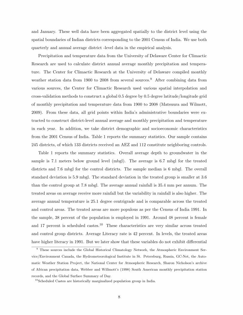
We first show that volume of cash crop exports from India did increase in response to

the AEZ policy. Figure 2 shows the volume of exports in metric tonnes over time. Before

2000-01, there is the data reveal no systematic pattern. After the announcement of the policy

in 2000-01, the volume of APEDA- approved cash crops increases systematically. APEDA

does not provide cluster or district-specific export figures. Hence we are unable to perform

district-level regression analysis. 16

Next we turn to exploring the effect of AEZs on groundwater depth. We use approval

dates as the time of treatment, but results are similar if we use the date of signing of the MOU

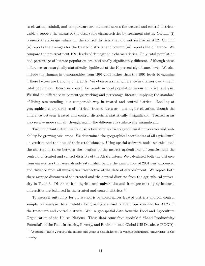
with the national government as the treatment date. We plot the raw data for treated and

comparison districts by quarter since the AEZ approval in Figure 3. Two notable features

are worth highlighting in this graph. First, the trends in groundwater depth in treated

and comparison districts before the AEZ policy were parallel. Second, before the AEZ was

approved, the depth to groundwater in treated districts was closer to the surface than in the

comparison group. After the AEZ, this wedge closed and the depth for the treated group

exceeded the comparison group in approximately four quarters (approximately one harvest

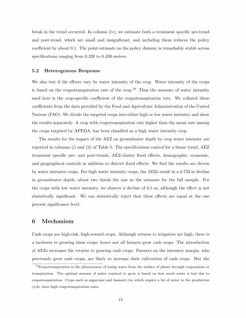
cycle). Figure 4 shows our results on groundwater. We represent quarters before and after

16Also, due to data limitations on crop-production data for cash crops, we are not able to estimate district-

specific changes in cash-crop production.

13

the passage of AEZ on the X axis. We plot the DID coefficients from a simple benchmark

specification that compares the log of annual depth to groundwater (where increases means

depletion of groundwater) in treated districts to their immediate neighbors controlling for

district fixed effects, AEZ-cluster fixed effects, quarter-of-year fixed effects, time trend, and

other time-variant characteristics of the districts. Before any AEZs were established, to the

left of 0, we see no effect on groundwater depth. However, after the AEZs were implemented,

we observe a decline in groundwater in the treated areas. This decline increases with passage

of time since the AEZs establishment.17These results are large in a small number of AEZs

where more than 12 quarters have elapsed since the establishment of an AEZ. In results not

shown, we find that estimates using a sample that excludes these AEZs (which have been

established for more than 12 quarters) are nearly identical to the ones from full sample.

We report the results from the regression analysis in Table 4. Each specification con-

trols for demographic, economic, and geographical characteristics of districts including total

population, literate population, fraction of working population, fraction of scheduled caste

population, and average annual rainfall and temperature.18 Each specification also includes

AEZ-cluster fixed effects, quarter fixed effects, and district fixed effects. Column (i) is the

most parsimonious specification, where we include a simple policy indicator equal to 1 in the

post-treatment period for treated districts. The coefficient estimate suggests that AEZ ap-

proval results in a level shift of groundwater in the treated districts of about 0.3 meters away

from the surface. The coefficient is highly statistically significant. Because the within district

standard deviation is around 2.5 meters, this effect represents 0.12 of a standard deviation

increase in the depth to groundwater.

We add a linear trend in column (ii) to account for any secular changes in groundwater

over the period. The point estimate for the policy dummy does not change. In column (iii),

we examine the possibility that groundwater trends were different in the control group prior

to the policy introduction, but we do not find any evidence for differential pre-trends. The

point estimate is robust to controlling for pre-trends in groundwater data. In the final column

of Table 4, we investigate the possibility that, in addition to a level shift in groundwater, a

17We estimate the effects by quarters since establishment for both treated and control districts. The patterns

in the coefficients are similar to those in the raw data in Figure 3. In Figure 4, we show the differences in the

coefficients for treated and control districts.18 We have the demographic and economic data for the Census years and interpolate these variables for the

remaining years.

14

break in the trend occurred. In column (iv), we estimate both a treatment specific pre-trend

and post-trend, which are small and insignificant, and including them reduces the policy

coefficient by about 0.1. The point estimate on the policy dummy is remarkably stable across

specifications ranging from 0.320 to 0.439 meters.

5.2 Heterogenous Response

We also test if the effects vary by water intensity of the crop. Water intensity of the crops

is based on the evapotranspiration rate of the crop.19 Thus the measure of water intensity

used here is the crop-specific coefficient of the evapotranspiration rate. We collated these

coefficients from the data provided by the Food and Agriculture Administration of the United

Nations (FAO). We divide the targeted crops into either high or low water intensity and show

the results separately. A crop with evapotranspiration rate higher than the mean rate among

the crops targeted by APEDA, has been classified as a high water intensity crop.

The results for the impact of the AEZ on groundwater depth by crop water intensity are

reported in columns (i) and (ii) of Table 5. The specifications control for a linear trend, AEZ

treatment specific pre- and post-trends, AEZ-cluster fixed effects, demographic, economic,

and geographical controls in addition to district fixed effects. We find the results are driven

by water intensive crops. For high water intensity crops, the AEZs result in a 0.733 m decline

in groundwater depth, about two thirds the size as the estimate for the full sample. For

the crops with low water intensity, we observe a decline of 0.5 m, although the effect is not

statistically significant. We can statistically reject that these effects are equal at the one

percent significance level.

6 Mechanism

Cash crops are high-risk, high-reward crops. Although returns to irrigation are high, there is

a tacitness to growing these crops; hence not all farmers grow cash crops. The introduction

of AEZs increases the returns to growing cash crops. Farmers on the intensive margin, who

previously grew cash crops, are likely to increase their cultivation of cash crops. But the

19Evapotranspiration is the phenomenon of losing water from the surface of plants through evaporation or

transpiration. The optimal amount of water required to grow is based on how much water is lost due to

evapotranspiration. Crops such as sugarcane and basmati rice which require a lot of water in the production

cycle, have high evapotranspiration rates.

15

strong incentives driven by an increase in prices, may also lead to entry into cultivating cash

crops. When a large fraction of farmers enter this market, resource extraction increases. The

model presented here formalizes this hypothesis. We use the framework previously developed

and used by Brander and Taylor (1997) and Taylor (2011) to examine extraction of renewable

resources in the following model of entry and exit in Indian cash-crop production to explain

our empirical findings.

In the model, the farmers either decide to grow the cash crops being targeted by the AEZ

or traditional crops that they have experience growing. This implies that there is entry and

exit into the cash crop markets.20

Farmers’ land is differentially suited to growing cash crops but assumed to be equally

suitable for growing conventional crops. If the farmer decides to grow cash crops, they earn

pw in time dt, where p is the relative price of the cash crops and w is the amount of water

extracted. If they do not grow cash crops, they earn I. Suppose GW (t) is the stock of

groundwater available at time t and the productivity of land for cash crops is proportional to

the available stock. Then, a farmer with land productivity α will earn pw = p α GW (t) per

unit time. Assume that the distribution of productivity is F (α) where α ∈ [0, α] . Farmers

compare income from growing cash crops to income from growing conventional varieties to

determine whether they should enter the cash crop market and extract groundwater.

The marginal farmer who grows cash crops is given by: p α∗ GW = I

Farmers with productivity α > α∗ grow cash crops.

If the mass of farmers growing cash crops is N, and the total number of active farmers is

N [1 − F (α∗)], then NF (α∗) must grow conventional crops. Since α∗ > 0 , the conventional

crop is always produced. Assuming constant returns in the conventional crop, and choosing

units such that output equals labor input, I = 1 at all times.

Define 4W as the amount of groundwater extracted per unit time when the stock size is

GW , and farmers with productivity no less than α∗ are engaged in growing cash crops.

4W = N GW

∫ α

α∗αf(α)dα (2)

20We make a simplifying assumption that farmers have already sunk a well. We can endogenize the decision

to sink a well. The qualitative predictions would remain the same. Therefore, we abstain from introducing well

sinking as a choice in the model for the sake of brevity. The purpose of our model is to provide insights about

the mechanism driving our empirical findings, and our simple model captures the underlying mechanism.

16

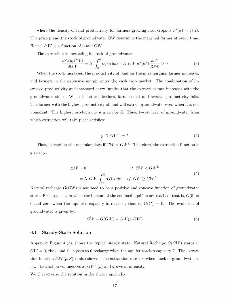
where the density of land productivity for farmers growing cash crops is F ′(α) = f(α).

The price p and the stock of groundwater GW determine the marginal farmer at every time.

Hence, 4W is a function of p and GW.

The extraction is increasing in stock of groundwater.

d4(p,GW )

dGW= N

∫ α

α∗αf(α)dα−N GW α∗(α∗)

dα∗

dGW> 0 (3)

When the stock increases, the productivity of land for the inframarginal farmer increases,

and farmers in the extensive margin enter the cash crop market. The combination of in-

creased productivity and increased entry implies that the extraction rate increases with the

groundwater stock. When the stock declines, farmers exit and average productivity falls.

The farmer with the highest productivity of land will extract groundwater even when it is not

abundant. The highest productivity is given by α. Thus, lowest level of groundwater from

which extraction will take place satisfies:

p α GWL = I (4)

Thus, extraction will not take place if GW < GWL. Therefore, the extraction function is

given by:

4W = 0 if GW < GWL

= N GW

∫ α

a∗αf(α)dα if GW ≥ GWL

(5)

Natural recharge G(GW) is assumed to be a positive and concave function of groundwater

stock. Recharge is zero when the bottom of the confined aquifers are reached; that is, G(0) =

0 and zero when the aquifer’s capacity is reached; that is, G(C) = 0. The evolution of

groundwater is given by:

˙GW = G(GW )−4W (p,GW ) (6)

6.1 Steady-State Solution

Appendix Figure 3 (a), shows the typical steady state. Natural Recharge G(GW ) starts at

GW = 0, rises, and then goes to 0 recharge when the aquifer reaches capacity C. The extrac-

tion function 4W (p, S) is also shown. The extraction rate is 0 when stock of groundwater is

low. Extraction commences at GWL(p) and grows in intensity.

We characterize the solution in the theory appendix.

17

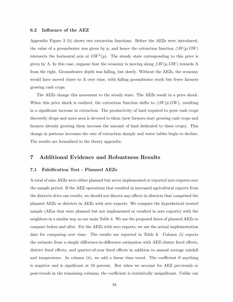
6.2 Influence of the AEZ

Appendix Figure 3 (b) shows two extraction functions. Before the AEZs were introduced,

the value of a groundwater was given by p, and hence the extraction function 4W (p;GW )

intersects the horizontal axis at GWL(p). The steady state corresponding to this price is

given by A. In this case, suppose that the economy is moving along 4W (p,GW ) towards A

from the right. Groundwater depth was falling, but slowly. Without the AEZs, the economy

would have moved closer to A over time, with falling groundwater stock but fewer farmers

growing cash crops.

The AEZs change this movement to the steady state. The AEZs result in a price shock.

When this price shock is realized, the extraction function shifts to 4W (p;GW ), resulting

in a significant increase in extraction. The productivity of land required to grow cash crops

discreetly drops and more area is devoted to them (new farmers start growing cash crops and

farmers already growing them increase the amount of land dedicated to these crops). This

change in patterns increases the rate of extraction sharply and water tables begin to decline.

The results are formalized in the theory appendix.

7 Additional Evidence and Robustness Results

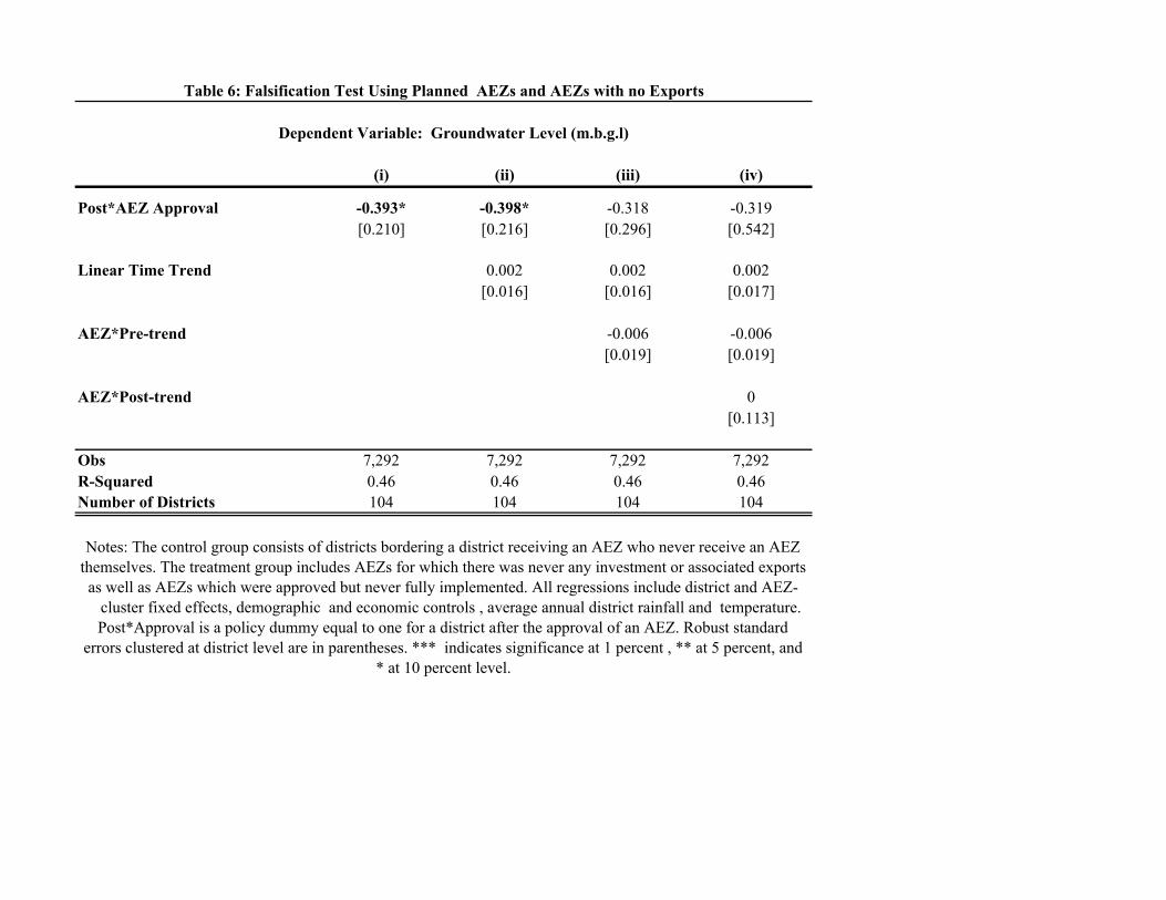
7.1 Falsification Test - Planned AEZs

A total of nine AEZs were either planned but never implemented or reported zero exports over

the sample period. If the AEZ operations that resulted in increased agricultural exports from

the districts drive our results, we should not discern any effects in districts that comprised the

planned AEZs or districts in AEZs with zero exports. We compare the hypothetical treated

sample (AEzs that were planned but not implemented or resulted in zero exports) with the

neighbors in a similar way as our main Table 4. We use the proposed dates of planned AEZs to

compare before and after. For the AEZs with zero exports, we use the actual implementation

date for comparing over time. The results are reported in Table 6. Column (i) reports

the estimate from a simple difference-in-difference estimation with AEZ-cluster fixed effects,

district fixed effects, and quarter-of-year fixed effects in addition to annual average rainfall

and temperature. In column (ii), we add a linear time trend. The coefficient if anything

is negative and is significant at 10 percent. But when we account for AEZ pre-trends or

post-trends in the remaining columns, the coefficient is statistically insignificant. Unlike our

18

main results, we observe a negative coefficient. These findings illustrate that an increase in

cash crop exports resulting from operations of AEZ are driving our results.

7.2 Are There Any Spill-Over Effects?

One possibility is that there are spatial spill-overs in our frame work. Economic spill-overs

can arise if increased returns to agricultural inputs in treated areas resulting from an increase

in exports changes the behavior of the farmers in the control areas. For example, there is a

movement of factors of production into treated areas from control areas. Also, hydrological

spill-overs from treated areas to their neighbors might occur. Given that lateral velocity of

groundwater is low (Todd, 1980), this scenario is less likely though still possible. In order

to examine these possibilities, we restrict our sample of treatment districts to those on the

cluster boundaries sharing a geographic border with the neighboring districts. If factors of

production move to the treated areas from the neighbors, we should see a larger effect in this

sample. If, on the other hand, the treated areas attract the groundwater from the control

areas, we should see a muted effect in this sample, and the magnitude should be smaller than

in the main sample. We report the results from this exercise in Table 7. Our most preferred

specification in column (iii) , where we report the results from a specification controlling AEZ-

cluster fixed effects, district fixed effects, quarter fixed effects, linear trend, and treatment

specific pre-trend in addition to annual average rainfall and temperature, finds that AEZs lead

to a decline of 0.491 m in the boundary sample. The coefficient from the same specification in

Table 4 yields an estimate of 0.413 which is also significant at 5 percent. These estimates are

not statistically distinguishable from each other. The test statistics testing for equivalence

of the interaction coefficients across Table 4 and 7 yield p-values of 0.4, 0.48, 0.4 and 0.15

across the four columns of the tables. Hence we cannot reject the null hypothesis that these

estimates are equal, and we do not find any evidence for spatial spill-overs.

7.3 Spatial Correlation across Districts

Geographical proximity of districts may result in spatial correlation in our application. Hence,

following Conley (1999), we allow for spatial correlation in our main empirical analysis. Dis-

tricts in India cover an expanse of around 66 kilometers on the average. Thus, we first allow

the spatial correlation to fall to 0 at a cutoff of 1 degree (latitude and longitude). This is

equivalent to around 111.3 km. The results from this estimation are reported in column (i) of

19

Appendix Table 3. As a sensitivity check, we also use 0.5 degrees (55.65 km) as the cutoff in

column (ii), and 1.5 degrees (166.95 km) in column (iii). The results are identical across these

columns using different cutoffs. The estimated coefficient of 0.43 is statistically significant at

5 percent. These results are the same as those reported in Table 4. Thus, our findings are

robust to allowing for spatial correlation.21

7.4 Using Variation in Timing of Introduction

The AEZ clusters did not start all at once. As Appendix Figure 1 shows, the timing of

introduction was staggered. Because state finance and budgetary considerations likely influ-

enced the timing, it is more likely to be endogenous. For example, states that were getting

richer could have implemented AEZs earlier than poorer states, and changes in standard of

living could have an independent effect on groundwater depth. Hence, we do not rely on this

variation for identification in our baseline results. We show that our results are invariant

qualitatively, and larger in magnitude in specifications comparing early versus late adopters,

but that early adoption is responsive to trends in economic variables. In this case, every

district in the sample would have received an AEZ, but the timing, and hence years of expo-

sure, would be different. Median number of clusters were set up by 2002. Hence we compare

districts in AEZ clusters set up before 2002 to ones set up after 2002.

We first compare the characteristics of districts that received the AEZs earlier (before

the median number were established) to neighboring districts that received it later. The

differences are reported in Appendix Table 4. As mentioned, we do see that these districts

are trending differently. Employment and literacy rates are increasing in early adopters. The

trends are modestly different and marginally significant. We replicate the specifications from

Table 4 and report the results in Appendix Table 5. In column (i), we show results from a

basic difference-in-difference model. In column(ii), we add a linear trend. In column (iii), we

add a treatment specific pre-trend. We add treatment specific pre- and post-trends in column

(iv). We find qualitatively similar results. Early adoption results in a 0.6 m greater decline in

groundwater depth. These results are stable across specifications and statistically significant

at the 1 percent level.

21We demeaned our data to carry out this analysis in order to control for district specific heterogeneity.

Conley’s (1999) algorithm to account for spatial correlation was implemented on the demeaned data.

20

7.5 Can Domestic Demand Have Driven the Results?

Because the Indian economy went through a period of rapid growth in the last decade, an

alternate explanation can be that domestic demand for agricultural products rose and thereby

accelerated groundwater decline. However, this explanation is not consistent with a number

of facts. First, the timing is inconsistent with this alternate hypothesis. The groundwater

depth declined in treated areas post AEZ establishment compared to years prior to AEZ

establishment. Not all AEZs were introduced at the same time. On the other hand, growth

rates over this period were high but steady and did not exhibit sharp temporal increases

(Virmani, 2009). Hence, increased domestic demand can have caused a gradual uniform shift

in groundwater depth but cannot explain a difference pre and post AEZ establishment over

multiple years. Second, we include linear time trends in our specifications to control for

universally experienced growth shocks. Thus, universal increases in demand cannot explain

our results. From Table 2, we see that treatment is uncorrelated with the change in rate of

employment. Standard of living in treated areas is similar to the control areas. Thus, local

growth shocks specific to the treatment areas cannot have generated demand for the goods

in question.22 In Table 5, our results vary by water intensity of crops and if local growth

generated our results, we would not expect this type of heterogeneity in our results. Finally

and most importantly, in Table 6, we show that the planned AEZs or AEZs that did not

result in any exports, did not affect groundwater depth. If local demand were driving the

results, we would see an effect in this case as well.

8 Income and Wages

The decline in depth to groundwater resulting from the establishment of AEZs should be

associated with an increase in incomes of individuals engaged in agriculture. From a policy

perspective, the impact on income is of interest for two reasons. First, illustrating the short-

term benefits is of first order importance from a public finance point of view. The cost of

provision of an agricultural export zone can be compared to these benefits to assess whether

these schemes make economic sense. Second, this exercise enables us to compare the ben-

22Local agriculture markets are spatially fragmented. Farmers from 2 to 3 villages sell to a wholesaler in

a nearby market called the ‘mandi’. These sales are often mediated by a middleman called the ‘artia’. The

wholesaler then sells to retailers. Produce is also sold at local village markets called the ‘haats’.

21

efits of the AEZ and the emergent increase in irrigation with the social cost resulting from

groundwater extraction.

We analyze the impact on mean expenditure per-capita using the following specification:

Idt = β0 +Ac +Dd + Post+ β1 Post ∗ T + β2 Xdt + νdt (7)

We estimate the model using district fixed effects (Dd), period fixed effect (Post) , and

AEZ- cluster fixed effects. Hence, the effect of the AEZ is identified entirely from variation

within districts over time that comprise specific AEZ clusters and their neighbors. We account

for common macro shocks affecting all districts. The district fixed effects control for time-

invariant characteristics of districts that make them suitable for both placement of an AEZ

and agriculturally productive so as to affect income. We show results both- with and without-

controlling for demographic and economic characteristics. We also examine the differential

impact on land-owning versus landless households. Hence, in the following variation of the

above specification, β4 is the parameter of interest.

Idt = β0+Ac+Dd+Post+β1 L+β2 Post∗T+β3Post∗L+β4 Post∗L∗T+β5 Xdt+νdt (8)

We use the nationally representative expenditure survey conducted by the National Sample

Survey Organization (NSSO) to estimate the effect on expenditures. The NSSO conducts

“thick rounds” every five years.23 We use the 1999 and 2009 rounds to conduct our analysis.

The AEZ policy was announced in 2001. Hence, we use 1999 as the pre year. We use repeated

cross-sections of the surveys to create a district-level panel. The NSSO data provide rural

wages, landholding status, occupation, and monthly mean per-capita expenditure (mpce).

We match these data to district level temperature and rainfall, and the groundwater depth

data.

Table 8 reports the results. The overall impact on monthly mean per-capita expenditure

is reported in columns (i) and (ii). The coefficient is 141 rupees without the demographic

controls and 126 with these controls. In both specifications, it is significant at the 10 percent

significance level. Columns (iii) through (vi) report the coefficients for landless and land-

owning households engaged in agriculture. The introduction of AEZs did not change the

expenditure profile of the landless households. The coefficients reported in columns (iii) and

23Thick rounds have larger sample sizes compared to thin rounds that are conducted every year.

22

(iv) are small and statistically insignificant. However, land-owning farmers did benefit. The

mpce increased by 147 rupees per month. The coefficients from both specifications (with and

without demographic controls) reported in columns (v) and (vi) are statistically significant

at the 5 percent significance level. The within district standard deviation over time is 537.94.

Hence, this effect is 0.3 of a standard deviation and is economically significant.

With the objective of examining whether small farmers benefitted differentially from large

farmers due to AEZ establishment, we also estimate heterogenous impacts by percentile of

land distribution within landowners. We split the land-owning sample below and above the

median of the land distribution in 1999. Thus, we compare households that own less than 2.04

hectares of land to those whose holdings are greater than 2.04 hectares. Columns (vi) through

(x) report the results. The impact on small and large farmers is positive and significant at

conventional levels of significance. We cannot reject the hypothesis that the coefficients are

equal (the p-value from the test of equivalence of (vi) and (ix) is 0.63 and for columns (viii)

and (x) is 0.634). Thus, we do not find evidence of small farmers benefitting differentially

relative to large farmers from the establishment of an AEZ in a district.

Next, we control for groundwater depth in the specifications to examine how much of

the variation in our mpce results is explained by changes in groundwater depth. The results

are reported in Table 9. The coefficient in columns (v) and (vi) are one-third in magnitude

and statistically insignificant in column (vi). Changes in groundwater depth cannot explain

around 37 percent of the variation in the results for the land-owning farmers (55.78 as a

percentage of 147.2). The increased extraction explains almost 62.2 percent of the variation

in the mpce. Thus, we can bound the benefit of a fall in groundwater depth of 0.4 meters

(reported in Table 4) at an increase of approximately 91 rupees in monthly mean per-capita

expenditure. This number represents 17.2 percent increase over the 1999 average for the

control group.24 Similarly, changes in groundwater depth explain 72 percent of the variation

in the effect on landowners with holdings greater than the median and 60 percent of the

24 If we assume that the depth goes down uniformly in the aquifers underlying the farms, then for the

median farmer with holdings of 2.04 hectares, a decline in depth of 0.4 meters will yield 8,160 cubic meters of

water. Groundwater for irrigation is not priced. Thus, if we further take the price of metered water provided

to households as the shadow price for water (provided at 10 rupees per liter in Chandigarh and 11 rupees in

Delhi), the social cost of groundwater extracted per household is fairly steep and could outweigh the realized

benefits. In order to explicitly do the cost-benefit analysis, we would need to specify the welfare function and

make assumptions about the rate of discounting over time.

23

variation for landowners with holdings smaller than the median. The coefficients reported in

columns (vii) through (x) are statistically insignificant when we control for changes in the

depth to groundwater. Overall, these findings indicate that changes in groundwater depth

are driving the results that we observe in Table 8, and change in the depth of groundwater

can be interpreted as a sufficient statistic in our analysis.

Finally, we examine the effect on rural agricultural wages. The results are reported in

Table 10. We find no effect of AEZ establishment on rural wages. The coefficients are

reported in columns (i) and (ii). The point estimates are small and statistically insignificant.

The impact on wages is small, insignificant, and statistically no different for landless and

land-owners. This finding is consistent with the results above that show no impact of the

AEZ on mpce for the landless households. Because wages are not changing in response to the

establishment of AEZ, the expenditure profile of landless households does not change either.

AEZs promote capital intensive agriculture, which might be primarily responsible for stable

wages over time.

9 Conclusion

Our paper investigates the effects of agricultural trade on groundwater depletion. Agricultural

trade is often promoted as an important lever to boost productivity and improve standards

of living in developing countries. Given the rapidly depleting groundwater resources around

the world that present a threat to food security, understanding how promoting agricultural

trade can affect groundwater stocks is vital.

We use the variation in trade introduced by the government of India’s 2001 exim policy

that set up agricultural trade promotion zones in various districts of India to promote the

trade of cash crops. We find that agricultural trade promotion exacerbates the depletion of

water tables in India. Our findings show that using trade promotion as a lever to increase

agricultural productivity can be counter productive in the long run if the institutional frame-

work for groundwater extraction remains unchanged. Groundwater shortages can reduce

agriculture production (Sekhri, 2013 b). In a property rights regime that allows for unlimited

access to groundwater conditional on landownership, such as exists in India, an increase in

international agricultural trade provides incentives to extract more groundwater. Institutions

that can promote resource management and conservation do not seem to have emerged.

24

References

[1] Bohn, H. and R. Deacon (2000), “Ownership Risk, Investment, and the Use of Natural

Resources”, The American Economic Review, Vol.90(3), pp.526-549

[2] Brander J.A. and M.S. Taylor (1997), “International Trade and Open Access Renewable

Resources: The Small Open Economy Case”, Canadian Journal of Economics, Vol. 30(3),

pp. 526-552

[3] Brander J.A. and M.S. Taylor(1998) , “The Simple Economics of Easter Island: A

Ricardo-Malthus Model of Renewable Resource Use,” American Economic Review, Vol.

88(1), pp. 119-138

[4] Bulte, E. and E. Barbier(2005), “Trade and Renewable Resources in a Second Best

World: An Overview”, Environmental and Resource Economics, Vol. 30(4), pp. 423-463

[5] Chichilnisky,G.(1994), “North-South Trade and the Global Environment”, Amreican

Economic Review,Vol. 84(4), pp. 851-874

[6] Conley, T. (1999), “GMM estimation with Cross Sectional Dependence”,Journal of

Econometrics,Vol. 92(1), pp. 1-45

[7] Copeland, B. and M.S. Taylor (2009), “Trade, Tragedy,and the Commons”, Amreican

Economic Review, Vol. 99(3), pp. 725-749

[8] Fischer, C. (2010), “ Does Trade Help or Hinder the Conservation of Natural Resources”,

Review of Environemntal Economics and Policy, Vol. 4(1), 103-121

[9] Foster, A. and M. Rosenzweig (2003) , “Economic Growth and the Rise of Forests” The

Quarterly Journal of Economics, Vol. 118(2), pp. 601-637

[10] Greenstone, M., R. Hornbeck, and E. Moretti(2010),“Identifying Agglomeration

Spillovers: Evidence from Winners and Losers of Large Plant Openings”, Journal of

Political Economy,Vol. 118(3),pp. 536-598

[11] Kremer, M. and C. Morcom (2000) , “Elephants,” American Economic Review vol. 90(1),

pp. 212-234

25

[12] Lopez, R.(1997),“Environmental externalities in traditional agriculture and the impact

of trade liberalization: the case of Ghana,” Journal of Development Economics, Vol.

53(1), pp. 17-39

[13] Lopez, R.(1998),“ The tragedy of the commons in Cote d’Ivoire agriculture: empiri-

cal evidence and implications for evaluating trade policies,”The World Bank Economic

Review Vol. 12(1), pp. 105-131

[14] Margolis,M. and J. Shogren(2002), “Unprotected Resources and Voracious World Mar-

kets,” Resources for the Future Discussion Paper 02-30

[15] Ostrom, E. (1990), Governing the Commons: The Evolution of Institutions for Collective

Action, Cambridge University Press: USA

[16] Ostrom, E. (2010), “Beyond Markets and States: Polycentric Governance of Complex

Economic Systems”, American Economic Review, Vol. 100(3), pp. 641-672

[17] Rodell, M., I. Velicogna, and J.Famiglietti (2009), “Satellite-based estimates of ground-

water depletion in India”, Nature, Vol. 460, pp. 999-1002

[18] Sekhri, S.(2012), “ Sustaining Groundwater: Role of Policy Reforms in Promoting Con-

servation” Forthcoming India Policy Forum

[19] Sekhri, S. (2013, a), “Missing Water: Agricultural Stress and Adaptation Strategies in

Response to Groundwater Depletion in India” Working paper

[20] Sekhri, S.(2013, b),“ Wells, Water, and Welfare: The Impact of Access to Groundwa-

ter on Rural Poverty and Conflict”, forthcoming American Economic Journal: Applied

Economics

[21] Taylor, S. (2011) ,“Buffalo Hunt International Trade and the Virtual Extinction of the

North American Bison” American Economic Review, Vol 101(7), pp. 3162-3195

[22] Virmani, A. (2009), “ India’s Growth Acceleration: The Third Phase !” OECD Data

Study

[23] Von Braun, J., M. Ruel, and A. Gulati (2008), “ Accelerating Progress Toward Reducing

Childhood Malnutrition in India,” Discussion paper, International Food Policy Research

Institute.

26

 

 Figure 1: AEZ clusters – in-sample treated and control districts along with the location of Agricultural Universities

 

Legend - AEZ-treated districts - Control districts - Agricultural Universities

 

                   

 

 

 

 ‐

 2,000,000

 4,000,000

 6,000,000

 8,000,000

 10,000,000

 12,000,000

Quan

tity in

 Metric Tons

Figure 2: Increase in Volume of Exports for APEDA Approved cash Crops

 

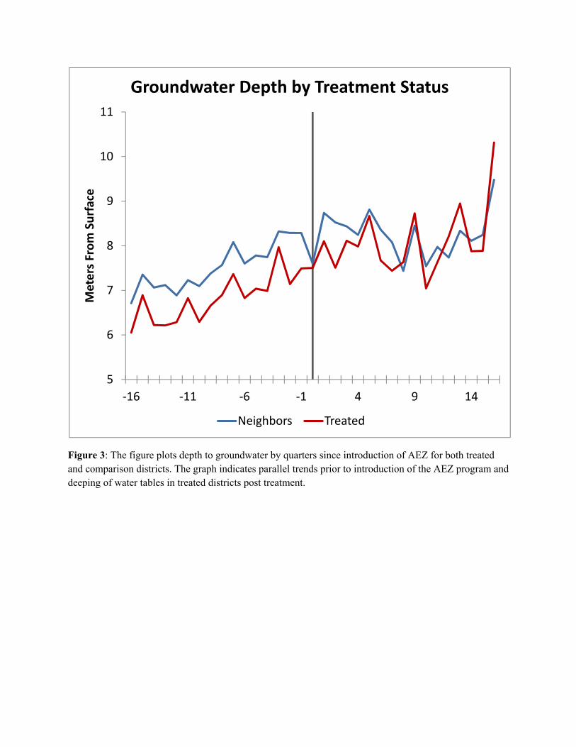
Figure 3: The figure plots depth to groundwater by quarters since introduction of AEZ for both treated and comparison districts. The graph indicates parallel trends prior to introduction of the AEZ program and deeping of water tables in treated districts post treatment.

 

5

6

7

8

9

10

11

‐16 ‐11 ‐6 ‐1 4 9 14

Meters From Surface

Groundwater Depth by Treatment Status

Neighbors Treated

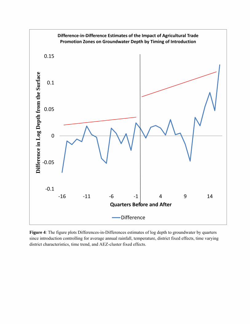
Figure 4: The figure plots Differences-in-Differences estimates of log depth to groundwater by quarters since introduction controlling for average annual rainfall, temperature, district fixed effects, time varying district characteristics, time trend, and AEZ-cluster fixed effects.

‐0.1

‐0.05

0

0.05

0.1

0.15

‐16 ‐11 ‐6 ‐1 4 9 14

Dif

fere

nce

in L

og D

epth

fro

m t

he

Su

rfac

e

Quarters Before and After

Difference‐in‐Difference Estimates of the Impact of Agricultural TradePromotion Zones on Groundwater Depth by Timing of Introduction

Difference

All DistrictsTreated Districts

Neighboring Districts

Average Groundwater Level Mean 7.1 6.7 7.6(meters from surface) Median 6.0 6.0 6.0

Std dev 5.9 3.6 7.8

Average rainfall Mean 35.3 37.5 32.7(meters/year) Median 17.8 19.9 15.8

Std dev 46.7 48.7 44.1

Average Temperature Mean 25.1 25.1 25.2(degrees celsius) Median 26.0 25.9 26.1

Std dev 4.4 4.2 4.6

1991 Population Mean 2,185 2,432 1,890(thousands) Median 2,117 2,334 1,882

Std dev 1,149 1,302 852

1991 Fraction SC Mean 0.17 0.16 0.17Median 0.16 0.16 0.17Std dev 0.07 0.08 0.07

1991 Fraction Literate Mean 0.42 0.45 0.40Median 0.40 0.44 0.38Std dev 0.14 0.15 0.13

1991 Fraction Working Mean 0.38 0.37 0.38Median 0.37 0.36 0.37Std dev 0.07 0.07 0.07

1991 Fraction Female Mean 0.48 0.48 0.48Median 0.48 0.48 0.48Std dev 0.02 0.02 0.02

Observations 245 133 112

Table 1: Summary Statistics

Average Depth to Groundwater

Overall Treated Neighbor Mean 6.9 6.3 7.5Median 5.8 5.9 5.6Std dev 7.1 3.1 9.9

Mean 6.6 6.2 7.0Median 5.8 5.9 5.8Std dev 5.0 3.0 6.7

Mean 6.1 5.7 6.6Median 5.3 5.4 5.1Std dev 4.8 2.7 6.5

Mean 6.5 6.2 6.9Median 5.5 5.5 5.5Std dev 5.1 3.1 6.8

Mean 6.9 6.5 7.4Median 5.8 5.9 5.8Std dev 5.9 3.4 7.9

Mean 7.4 7.0 7.9Median 6.3 6.2 6.4Std dev 6.0 3.8 7.9

Mean 7.8 7.4 8.2Median 6.6 6.6 6.6Std dev 5.9 3.9 7.6

Mean 7.9 7.5 8.3Median 6.6 6.6 6.6Std dev 6.3 4.0 8.2

Mean 7.9 7.5 8.3Median 6.7 6.7 6.8Std dev 6.3 4.0 8.1

Mean 7.5 7.3 7.8Median 6.2 6.1 6.3Std dev 6.0 4.3 7.4

1997

1996

2004

2005

1998

1999

2000

2001

2002

2003

Table 2: Summary Statistics by Year

Untreated Treated Difference

Population 1890.47 2432.42 551.59*

Percent SC 0.17 0.16 0.00

Percent Literate 0.40 0.45 .05*

Percent Working 0.38 0.37 0.00

Percent Female 0.48 0.48 0.00

Population 103.70 363.94 260.23*

Percent SC 0.00 0.00 0.00

Percent Literate 0.12 0.12 -0.01

Percent Working 0.02 0.02 -0.01

Percent Female 0.00 0.00 0.00

0.57 0.58 0.01

Distance from Pre-existing Agricultural 0.72 0.62 -0.10Universities

272.13 287.17 15.03

33.26 37.84 4.58

25.08 25.03 -0.05

5.49 5.65 0.15

0.56 0.29 -0.28

7.48 6.62 -0.86

112 133 --

Change in Demographics, 1991-2001

Table 3: Characteristics Influencing Selection of Treated Districts

Demographics, Levels 1991

Distance from Agricultural Universities

Elevation

Notes: Average Crop suitability based on suitability measures for onion, rice, potato, banana, citrus, flower, vegetable, fruit and wheat. * indicates p<.05

Number of Districts

Rainfall

Temperature

Average Suitability for Certain Crops

Change In groundwater Level, '99-00

Average Groundwater Level

Dependent Variable: Groundwater Level (m.b.g.l)

(i) (ii) (iii) (iv)

Post*AEZ Approval 0.305* 0.320* 0.413** 0.439**[0.171] [0.182] [0.172] [0.204]

Linear Time Trend -0.005 -0.002 -0.002[0.015] [0.017] [0.017]

AEZ*Pre-trend -0.011 -0.011[0.014] [0.014]

AEZ*Post-trend -0.004[0.031]

Obs 14,629 14,629 14,629 14,629R-Squared 0.24 0.24 0.24 0.24Number of Districts 246 246 246 246

Table 4: Impact of Agricultural Trade Promotion on Groundwater

Notes: The control group consists of districts bordering a district receiving an AEZ who never receive an AEZ themselves. The treatment group excludes AEZs for which there was never any investment or associated exports. All regressions include district and AEZ-cluster fixed effects, demographic and economic controls , average annual district rainfall and temperature. Post*Approval is a policy dummy equal to one for a district after the approval of an AEZ. Robust standard errors clustered at district level are in parentheses. *** indicates significance at 1 percent , ** at 5 percent, and * at 10 percent level.

Table 5: The Impact of Agricultural Trade Promotion on Groundwater by Crop Water Intensity

Low High

(i) (ii)

Post*AEZ Approval -0.573 0.733***[0.428] [0.192]

Linear Time Trend Yes Yes

AEZ*Pre-trend Yes Yes

AEZ*Post-trend Yes Yes

R-Squared 0.29 0.16Number of Districts 83 125

Notes: High water intensity crops have an evapotranspiration rate higher than the mean rate among targeted crops. All regressions include district and AEZ-cluster fixed effects, demographic and economic controls, average annual district rainfall and temperature. Robust standard errors clustered at district level are in parentheses. *** indicates significance at 1 percent , ** at 5 percent level , * at 10 percent

level.

Water Intensity

Dependent Variable: Groundwater Level (m.b.g.l)

Dependent Variable: Groundwater Level (m.b.g.l)

(i) (ii) (iii) (iv)

Post*AEZ Approval -0.393* -0.398* -0.318 -0.319[0.210] [0.216] [0.296] [0.542]

Linear Time Trend 0.002 0.002 0.002[0.016] [0.016] [0.017]

AEZ*Pre-trend -0.006 -0.006[0.019] [0.019]

AEZ*Post-trend 0[0.113]

Obs 7,292 7,292 7,292 7,292R-Squared 0.46 0.46 0.46 0.46Number of Districts 104 104 104 104

Table 6: Falsification Test Using Planned AEZs and AEZs with no Exports

Notes: The control group consists of districts bordering a district receiving an AEZ who never receive an AEZ themselves. The treatment group includes AEZs for which there was never any investment or associated exports as well as AEZs which were approved but never fully implemented. All regressions include district and AEZ-

cluster fixed effects, demographic and economic controls , average annual district rainfall and temperature. Post*Approval is a policy dummy equal to one for a district after the approval of an AEZ. Robust standard

errors clustered at district level are in parentheses. *** indicates significance at 1 percent , ** at 5 percent, and * at 10 percent level.

Dependent Variable: Groundwater Level (m.b.g.l)

(i) (ii) (iii) (iv)

Post*AEZ Approval 0.380** 0.378* 0.491** 0.668***[0.188] [0.198] [0.197] [0.171]

Linear Time Trend 0.001 0.003 0.004[0.017] [0.018] [0.018]

AEZ*Pre-trend -0.012 -0.013[0.014] [0.014]

AEZ*Post-trend -0.025[0.031]

Obs 12,950 12,950 12,950 12,950R-Squared 0.24 0.24 0.24 0.24Number of Districts 216 216 216 216

Table 7: Impact of Agricultural Trade Promotion on Groundwater Along Cluster Boundaries

Notes: The control group consists of districts bordering a district receiving an AEZ who never receive an AEZ themselves. The treatment group excludes AEZs for which there was never any investment or associated exports. All regressions include district and AEZ-cluster fixed effects, demographic and economic controls , average annual district rainfall and temperature. Post*Approval is a policy dummy equal to one for a district after the approval of an AEZ. Robust standard errors clustered at district level are in parentheses. *** indicates significance at 1 percent , ** at 5 percent, and * at 10 percent level.

Dependent Variable: Mean Monthly Per Capita Expenditure

(i) (ii) (iii) (iv) (v) (vi) (vii) (viii) (ix) (x)

AEZ * Post 141.3* 126.3* 16.63 27.41 168.5** 147.2** 184.3** 164.0** 160.4** 140.8*(76.03) (68.77) (146.4) (147.8) (69.22) (59.60) (83.60) (73.33) (79.90) (72.34)

District-level Demographic No Yes No Yes No Yes No Yes No Yes

Observations 97,707 85,523 3,420 3,103 94,181 82,339 40,647 35,776 53,534 46,563R-squared 0.047 0.044 0.447 0.518 0.047 0.044 0.021 0.021 0.219 0.220

*** indicates significance at 1 percent , ** at 5 percent, and * at 10 percent level.The outcome variable is the mean per capita expenditure within household. Robust standard errors are clustered at district level and reported in parentheses. Post is an indicator that equals to 1 for 2009 and 0 for 1999. Every regression controls for district fixed effects, post indicator, AEZ- cluster fixed effect, district level average rainfall and temperature. Demographic controls include total population of the district, percentage of working population, and percentage of literature population interacted with post.

Table 8: Impact of Agricultural Trade Promotion on Per Capita Expenditure

All Observations Landless Land-owners 50-100 percentile0-50 percentileLand Holdings > 2.04

haLand Holdings 0.01 - 2.04 ha

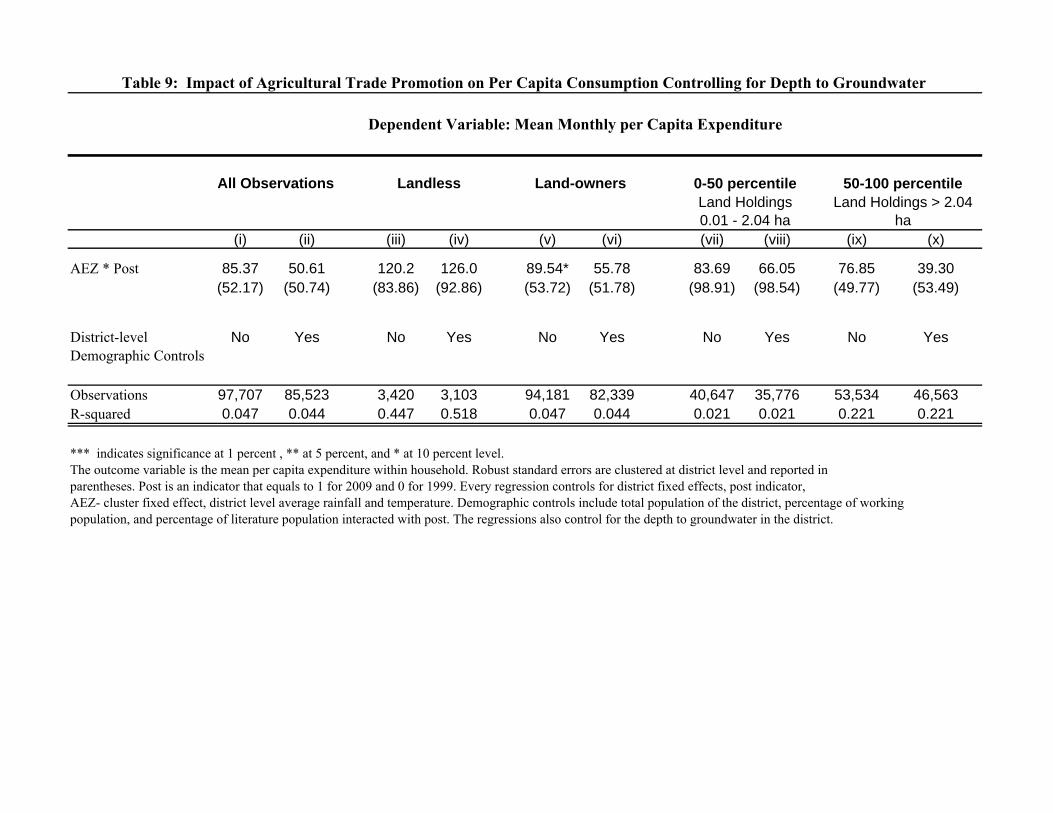
Dependent Variable: Mean Monthly per Capita Expenditure

(i) (ii) (iii) (iv) (v) (vi) (vii) (viii) (ix) (x)

AEZ * Post 85.37 50.61 120.2 126.0 89.54* 55.78 83.69 66.05 76.85 39.30(52.17) (50.74) (83.86) (92.86) (53.72) (51.78) (98.91) (98.54) (49.77) (53.49)

District-level Demographic Controls

No Yes No Yes No Yes No Yes No Yes

Observations 97,707 85,523 3,420 3,103 94,181 82,339 40,647 35,776 53,534 46,563R-squared 0.047 0.044 0.447 0.518 0.047 0.044 0.021 0.021 0.221 0.221

*** indicates significance at 1 percent , ** at 5 percent, and * at 10 percent level.The outcome variable is the mean per capita expenditure within household. Robust standard errors are clustered at district level and reported in parentheses. Post is an indicator that equals to 1 for 2009 and 0 for 1999. Every regression controls for district fixed effects, post indicator, AEZ- cluster fixed effect, district level average rainfall and temperature. Demographic controls include total population of the district, percentage of working population, and percentage of literature population interacted with post. The regressions also control for the depth to groundwater in the district.

Land Holdings 0.01 - 2.04 ha

Land Holdings > 2.04 ha

Table 9: Impact of Agricultural Trade Promotion on Per Capita Consumption Controlling for Depth to Groundwater

All Observations Landless Land-owners 0-50 percentile 50-100 percentile

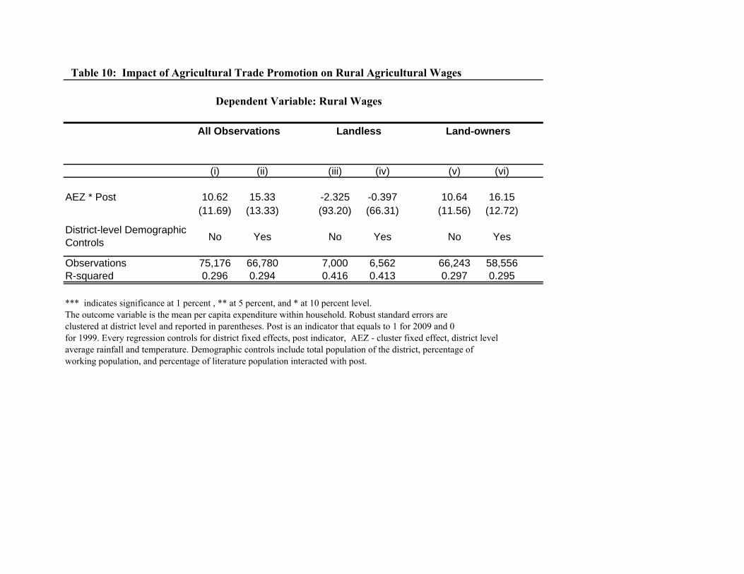
Table 10: Impact of Agricultural Trade Promotion on Rural Agricultural Wages

Dependent Variable: Rural Wages

(i) (ii) (iii) (iv) (v) (vi)

AEZ * Post 10.62 15.33 -2.325 -0.397 10.64 16.15(11.69) (13.33) (93.20) (66.31) (11.56) (12.72)

District-level Demographic Controls No Yes No Yes No Yes

Observations 75,176 66,780 7,000 6,562 66,243 58,556R-squared 0.296 0.294 0.416 0.413 0.297 0.295

*** indicates significance at 1 percent , ** at 5 percent, and * at 10 percent level.The outcome variable is the mean per capita expenditure within household. Robust standard errors areclustered at district level and reported in parentheses. Post is an indicator that equals to 1 for 2009 and 0for 1999. Every regression controls for district fixed effects, post indicator, AEZ - cluster fixed effect, district level average rainfall and temperature. Demographic controls include total population of the district, percentage of working population, and percentage of literature population interacted with post.

All Observations Landless Land-owners

Supplemental Material: Online Appendix

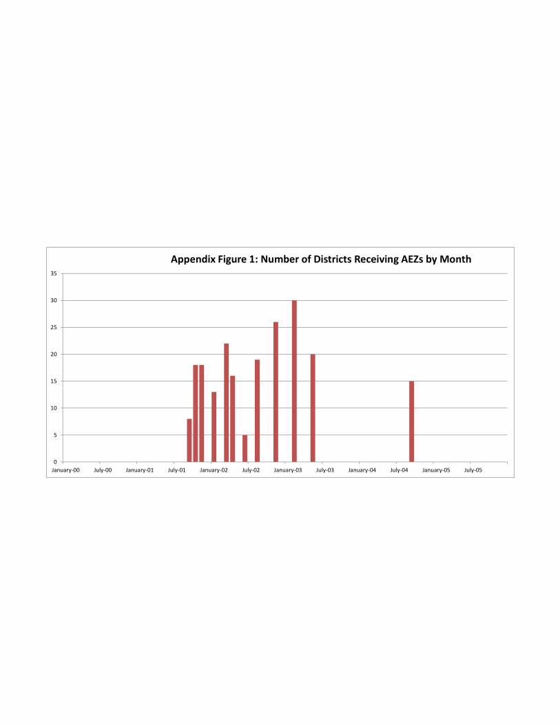
15

20

25

30

35

Appendix Figure 1: Number of Districts Receiving AEZs by Month

0

5

10

January‐00 July‐00 January‐01 July‐01 January‐02 July‐02 January‐03 July‐03 January‐04 July‐04 January‐05 July‐05

 

 

Appendix Figure 2: AEZ clusters – in-sample treated and comparison districts along with the location of Agricultural Universities separated by year of establishment 

Legend

- AEZ-treated districts - Control districts - Control districts with missing data - Agricultural Universities established prior to 2001 - Agricultural Universities established after 2001

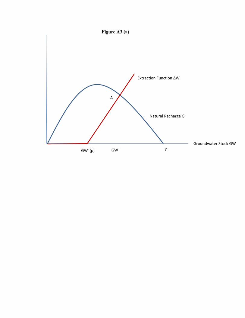
                                                                         Figure A3 (a)

A

Groundwater Stock GW 

Extraction Function ΔW 

Natural Recharge G 

GWL (p)  GW*  C

                                                                           Figure A3 (b) 

A

B 

Ground Water Stock GW

GW* GW*’  C 

G(GW) 

ΔW(p,GW) 

ΔW(p’,GW) 

GWL (p) GWL (p’) 

S. No Product State District/Area

Date of Approval

Date of Signing of

MOU

Planned Percentage of Expenditures

by Government

1 Pineapple West Bengal Darjeeling, Uttar Dinajpur, Cooch Behar and Jalpaiguri 7-Sep-01 18-Sep-01 11.7

2 Gherkins Karnataka

Tumkur, Bangalore Urban, Bangalore Rural, Hassan, Kolar, Chtradurga, Dharwad and Bagalkot 7-Sep-01 19-Sep-01 29.2

3 Lychee Uttaranchal Udhamsingh Nagar, Nainital and Dehradun 7-Sep-01 22-Sep-01 60.5

4 Vegetables Punjab Fatehgarh Sahib, Patiala, Sangrur, Ropar & Ludhiana 11-Oct-01 29-Oct-01 44.2

5 Potatoes Uttar Pradesh

Agra, Hathras, Farrukhabad, Kannoj, Meerut, Aligarh and Bagpat 11-Oct-01 7-Nov-01 88.1

6Mangoes and Vegetables Uttar Pradesh

Lucknow, Unnao, Hardoi, Sitapur & Barabanki 11-Oct-01 7-Nov-01 36.9

7 Potatoes Punjab

Singhpura, Zirakpur (Patiala), Rampura Phul, Muktsar, Ludhiana, Jallandhar 27-Nov-01 20-Dec-01 78.7

8 Mangoes Uttar Pradesh

Sahranpur, Muzaffarnagar, Bijnaur, Meerut, Baghpat, Bulandshar and Jyotifulenagar 27-Nov-01 21-Dec-01 52.4

9Grapes and Grape Wine Maharashtra

Nasik, Sangli, Pune, Satara, Ahmednagar and Sholapur 27-Nov-01 7-Jan-02 100.0

Table A1: Catalog of Agri Export Zones and Associated Exports/Expenditures

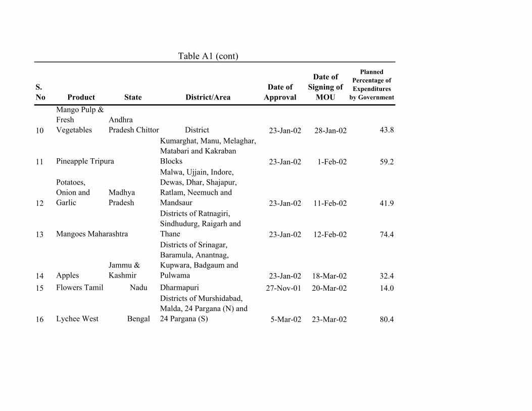
Table A1 (cont)

S. No Product State District/Area

Date of Approval

Date of Signing of

MOU

Planned Percentage of Expenditures

by Government

10

Mango Pulp & Fresh Vegetables

Andhra Pradesh Chittor District 23-Jan-02 28-Jan-02 43.8

11 Pineapple Tripura

Kumarghat, Manu, Melaghar, Matabari and Kakraban Blocks 23-Jan-02 1-Feb-02 59.2

12

Potatoes, Onion and Garlic

Madhya Pradesh

Malwa, Ujjain, Indore, Dewas, Dhar, Shajapur, Ratlam, Neemuch and Mandsaur 23-Jan-02 11-Feb-02 41.9

13 Mangoes Maharashtra

Districts of Ratnagiri, Sindhudurg, Raigarh and Thane 23-Jan-02 12-Feb-02 74.4

14 Apples Jammu & Kashmir

Districts of Srinagar, Baramula, Anantnag, Kupwara, Badgaum and Pulwama 23-Jan-02 18-Mar-02 32.4

15 Flowers Tamil Nadu Dharmapuri 27-Nov-01 20-Mar-02 14.0

16 Lychee West Bengal

Districts of Murshidabad, Malda, 24 Pargana (N) and 24 Pargana (S) 5-Mar-02 23-Mar-02 80.4

Table A1 (cont)

S. No Product State District/Area

Date of Approval

Date of Signing of

MOU

Planned Percentage of Expenditures

by Government

17 Lychee Bihar

Muzaffarpur, Samastipur, Hajipur, Vaishali, East and West Champaran, Bhagalpur, Begulsarai, Khagaria, Sitamarhi, Sarannd Gopalganj 5-Mar-02 5-Apr-02 38.2

18 Kesar Mango Maharashtra

Districts of Aurangabad, Jalna, Beed, Latur, Ahmednagar and Nasik 5-Mar-02 11-Apr-02 40.8

19 Walnut Jammu & Kashmir

Kashmir Region – Baramulla, Anantnag, Pulwama, Budgam, Kupwara and Srinagar / Jammu Region - Doda, Poonch, Udhampur, Rajouri and Kathua 5-Mar-02 11-May-02 47.0

20 Flowers Uttranchal Districts of Dehradun, Pantnagar 23-Apr-02 30-May-02 21.7

21Mangoes & Vegetables Gujarat

Districts of Ahmedabad, Khaida, Anand, Vadodra, Surat, Navsari, Valsad, Bharuch and Narmada 23-Apr-02 30-May-02 45.6

22 Flowers Maharashtra Pune, Nasik, Kolhapur and Sangli 5-Mar-02 10-Jun-02 54.2

S. No Product State District/Area

Date of Approval

Date of Signing of

MOU

Planned Percentage of Expenditures

by Government

23 Potatoes West Bengal

Districts of Hoogly, Burdwan, Midnapore (W), Uday Narayanpur and Howrah 23-Apr-02 18-Jun-02 22.0

24 Rose Onion Karnataka Bangalore (Urban), Bangalore (Rural), Kolar 13-Jun-02 1-Jul-02 40.7

25 Flowers Karnataka

Bangalore (Urban), Bangalore (Rural), Kolar, Tumkur, Kodagu and Belgaum 13-Jun-02 1-Jul-02 65.2

26Mango & Grapes

Andhra Pradesh

Districts of Ranga Reddy, Medak & Parts of Mahaboobnagar Districts 23-Apr-02 29-Jul-02 27.0

27

Flowers (Orchids) & Cherry Pepper Sikkim East Sikkim 13-Jun-02 26-Aug-02 32.5

28 Ginger Sikkim North, East, South & West 13-Jun-02 26-Aug-02 68.0

29 Apples Himachal Pradesh

Shimla, Sirmour, Kullu, Mandi, Chamba and Kinnaur 28-Aug-02 17-Sep-02 48.3

30 Basmati Rice Punjab

Districts of Gurdaspur, Amritsar, Kapurthala, Jalandhar, Hoshiarpur and Nawanshahar 28-Aug-02 17-Sep-02 58.8

Table A1 (cont)

S. No Product State District/Area

Date of Approval

Date of Signing of

MOU

Planned Percentage of Expenditures

by Government

31 Mangoes Andhra Pradesh Krishna District 28-Aug-02 27-Sep-02 44.7

32 Flowers Tamilnadu Nilgiri District 28-Aug-02 6-Feb-03 45.5

33 Onion Maharashtra

Districts of Nasik, Ahmednagar, Pune, Satara and Solapur 18-Nov-02 16-Jan-03 59.3

34Ginger and Turmeric Orissa Kandhamal District 18-Nov-02 10-Jan-03 49.8

35 Vegetables Jharkhand Ranchi, Hazaribagh and Lohardaga 18-Nov-02 15-Feb-03 54.4

36 Seed Spices Madhya Pradesh

Guna, Mandsaur, Ujjain, Rajgarh, Ratlam, Shajapur and Neemuch 18-Nov-02 28-Nov-02 51.6

37 Basmati Rice Uttaranchal

Udham Singh Nagar, Nainital, Dehradun and Haridwar 18-Nov-02 24-Jan-03 48.5

38 Mangoes West Bengal Malda and Murshidabad 18-Nov-02 16-Dec-02 41.5

39 Vegetables West Bengal Nadia, Murshidabad and North 24 Parganas 18-Nov-02 16-Dec-02 25.2

40 Mangoes Tamil Nadu

Districts of Madurai, Theni, Dindigul, Virudhunagar and Tirunelveli 18-Nov-02 6-Feb-03 43.4

Table A1 (cont)

S. No Product State District/Area

Date of Approval

Date of Signing of

MOU

Planned Percentage of Expenditures

by Government

41 Wheat Madhya Pradesh

Three distinct and contiguous zones:- Ujjain Zone comprising of Neemach, Ratlam, Mandsaur and Ujjain / Indore Zone comprising of Indore, Dhar, Shajapur and Dewas / Bhopal Division, comprising of Sehore, Vidisha, Raisen, Hoshangabad, Harda, Narsinghpur and Bhopal 28-Aug-02 16-Jan-03 42.3

42Horticulture Products Kerala

Districts of Thrissur, Ernakulam, Kottayaam, Alappuzha, Pathanumthitta, Kollam, Thiruvanthapuram, Idukki and Palakkod 3-Feb-03 5-Mar-03 60.3

43

Fresh & Processed Ginger Assam

Kamrup, Nalbari, Barpeta, Darrang, Nagaon, Morigaon, Karbi Anglong and North Cachar districts 3-Feb-03 4-Apr-03 41.1

Table A1 (cont)

S. No Product State District/Area

Date of Approval

Date of Signing of

MOU

Planned Percentage of Expenditures

by Government

44 Basmati Rice Uttar Pradesh

Districts of Bareilly, Shahajahanpur, Pilibhit, Rampur, Badaun, Bijnor, Moradabad, J B Phulenagar, Saharanpur, Mujjafarnagar, Meerut, Bulandshahar, Ghaziabad 3-Feb-03 11-Mar-03 50.9

45

Medicinal & Aromatic Plants Uttranchal

Districts of Uttarkashi, Chamoli, Pithoragarh, Dehradun and Nainital 3-Feb-03 26-Mar-03 51.9

46Dehydrated Onion Gujarat

Districts of Bhavnagar, Surendranagar, Amreli, Rajkot, Junagadh and Jamnagar. 5-May-03 10-Jun-03 47.7

47 Gherkins Andhra Pradesh

Districts of Mahboobnagar, Rangareddy, Medak, Karinagar, Warangal, Ananthpur and Nalgonda 5-May-03 12 May, 2003 18.6

48 Pomegranate Maharashtra

Districts of Solapur, Sangli, Ahedabagar, Pune, Nasik, Osmanabad, Latur 5-May-03 9 June, 2003 52.5

49 Banana Maharashtra

Jalgaon, Dhule, Nandurbar, Buldhana, Parbhani, Hindoli, Nanded and Wardha 24-Sep-04 - 43.0

50 Oranges Maharashtra Nagpur and Amraoti 24-Sep-04 - 47.2

Table A1 (cont)

S. No Product State District/Area

Date of Approval

Date of Signing of

MOU

Planned Percentage of Expenditures

by Government

51Lentil and Grams

Madhya Pradesh

Shivpuri, Guna, Vidisha, Raisen, Narsinghpura, Chhindwara 24-Sep-04 - 39.6

52 Oranges Madhya Pradesh

Chhindwara, Hoshangabad, Betul 24-Sep-04 - 43.9

53 Cashewnut Tamil Nadu Cuddalore, Thanjavur, Pudukottai and Sivaganga 24-Sep-04 - 40.6

60 Chilli Andhra Guntur 24-Sep-04 29-Dec-05 37.8

Table A1 (cont)

Table A2: Agricultural Universities by Years of EstablishmentYear of

Name District State Establishment

Acharya NG Ranga Agricultural University Hyderabad Andra Pradesh 1964

Anand Agricultural University formerly Gujarat Agricultural University Anand Gujarat 1972

Assam Agricultural University Jorhat Assam 1969

Bidhan Chandra Krishi Viswavidyalaya Nadia West Bengal 1974

Bihar Agricultural University Bhagalpur Bihar 2010

Birsa Agricultural University Ranchi Jharkhand 1981

Central Agricultural University Imphal Manipur 1992

Chandra Shekar Azad University of Agriculture & Technology Kanpur Uttar Pradesh 1975

Chaudhary Charan Singh Haryana Agricultural University Hisar Haryana 1970

CSK Himachal Pradesh Krishi Vishvavidyalaya Palampur Himachal Pradesh 1978

Chhattisgarh Kamdhenu Vishwavidyalaya Durg Chattisgarh 2012

Dr Balasaheb Sawant Konkan Krishi Vidyapeeth Ratnagiri Maharashtra 1972

Dr Panjabrao Deshmukh Krishi Vidyapeeth Akola Maharashtra 1969

Dr Yashwant Singh Parmar Univ of Horticulture & Forestry Solan Himachal Pradesh 1988

Dr YSR Horticultural University West Godavari Andra Pradesh 2007

Govind Ballabh Pant University of Agriculture & Technology Udham Singh Uttranchal 1960

Nagar

Guru Angad Dev Veterinary and Animal Science University Ludhiana Punjab 2005

Indira Gandhi Krishi Vishwavidyalaya Rai Pur Chattisgarh 1987

Jawaharlal Nehru Krishi Viswavidyalaya Jabalpur Madhya Pradesh 1964

Junagadh Agricultural University Junagarh Gujarat 1972

Karnataka Veterinary, Animal and Fisheries Sciences University Bidar Karnataka 2005

Kerala Agricultural University Trichur Kerala 1971

Kerala University of Fisheries & Ocean Studies Kochi Kerala 1979

Kerala Veterinary and Animal Sciences University Thiruvananthapuram Kerala 2010

Lala Lajpat Rai University of Veterinary & Animal Sciences Hisar Haryana 2010

Nanaji Deshmukh Veterinary Science University Jabalpur Madhya Pradesh 2009

Maharana Pratap Univ. of Agriculture & Technology Udaipur Rajasthan 1999

Maharashtra Animal Science & Fishery University Nagpur Maharashtra 2000

Mahatma Phule Krishi Vidyapeeth Rahuri Maharashtra 1969

Manyavar Shri Kanshiram Ji University of Agriculture and Technology Banda Uttar Pradesh 2010

Marathwada Agricultural University Parbhani Maharashtra 1972

Narendra Deva University of Agriculture & Technology Faizabad Uttar Pradesh 1974

Navsari Agricultural University, formerly Gujarat Agriculture University Navsari Gujarat 1972

Orissa University of Agriculture & Technology Bhubaneshwar Orrisa 1962

Punjab Agricultural University Ludhiana Punjab 1962

Rajasthan University of Veterinary and Animal Sciences Bikaner Rajasthan 2010

Rajendra Agricultural University Samistipur Bihar 1970

Rajmata Vijayraje Sciendia Krishi Vishwa Vidyalaya Gwalior Madhya Pradesh 2008

Sardar Vallabhbhai Patel University of Agriculture and Technology Meerut Uttar Pradesh 2000

Sardarkrushinagar-Dantiwada Agricultural University Banaskantha Gujarat 1972

Sher-E-Kashmir Univ of Agricultural Sciences & Technology Jammu Jammu and Kashmir 1998

Sher-E-Kashmir Univ of Agricultural Sciences & Technology of Kashmir Srinagar Jammu and Kashmir 1992

Sri Venkateswara Veterinary University Tirupati Andra Pradesh 2005

Swami Keshwanand Rajasthan Agricultural University Bikaner Rajasthan 1987

Tamil Nadu Agricultural University Coimbatore Tamil Nadu 1971

Tamil Nadu Fisheries University Nagapattinam Tamil Nadu 2012

Tamil Nadu Veterinary & Animal Science University Chennai Tamil Nadu 1989

University of Agricultural Sciences, Bangalore Begaluru Karnataka 1963

University of Agricultural Sciences, Dharwad Dharwand Karnataka 1986

University of Agricultural Sciences, Shimoga Shimoga Karnataka 1963

University of Horticultural Sciences Bagalkot Karnataka 2008

University of Agricultural Sciences Raichur Karnataka 2009

UP Pandit Deen Dayal Upadhaya Pashu Chikitsa Vigyan Mathura Uttar Pradesh 2001

Vishwa Vidhyalaya evam Go Anusandhan Sansthan

Uttarakhand University of Horticulture and Forestry Pauri Garhwal Uttrakhand 2011

Uttar Banga Krishi Viswavidyalaya Cooch Bihar West Bengal 2001

West Bengal University of Animal & Fishery Sciences Calcutta West Bengal 1995

Table A3 : Impact of Agricultural Trade Promotion on Groundwater Allowing for Spatial Correlation

Dependent Variable: Groundwater Level (m.b.g.l)

(i) (ii) (iii)

Cutoff 1 degree 0.5 degrees 1.5 degrees

Post*AEZ Approval 0.438** 0.438** 0.43**(0.21) (0.20) (0.23)

Linear Time Trend Yes Yes Yes

AEZ*Pre-trend Yes Yes Yes

AEZ*Post-trend Yes Yes Yes

Obs 14,629 14,629 14,629

Notes: The control group consists of districts bordering a district receiving an AEZ who never receive an AEZ themselves. The treatment group excludes AEZs for which there was never any investment or associated exports. De-meaned data are used to account for district fixed effects. All regressions include AEZ-cluster fixed effects, demographic and economic

controls , average annual district rainfall and temperature. Post*Approval is a policy dummy equal to one for a district after the approval of an AEZ. Spatial errors are in parentheses. *** indicates significance at 1 percent , ** at 5 percent, and * at

10 percent level.

Untreated Treated Difference

Population 2267.99 2582.90 314.91*

Percent SC 0.15 0.18 0.03*

Percent Literate 0.48 0.43 -0.05*

Percent Working 0.39 0.38 -0.01

Percent Female 0.49 0.48 -0.01

Population 275.23 392.47 117.24*

Percent SC 0.00 0.00 -0.00*

Percent Literate 0.10 0.13 0.03*

Percent Working 0.00 0.02 0.02*

Percent Female 0.00 0.00 0.00

0.59 0.56 -0.03

365.32 315.48 -49.84

38.52 34.34 -4.18

25.19 25.03 -0.15

6.35 5.56 -0.79*

0.14 0.32 0.18

6.95 6.96 0.01

19 96 --

Table A4: Characteristics Influencing Selection of Early Adopters

Demographics, Levels 1991

Average Groundwater Level

Number of DistrictsNotes: Average Crop suitability based on suitability measures for onion, rice, potato, banana, citrus, flower, vegetable, fruit and wheat. * indicates p<.05

Average Suitability for Certain Crops

Change In groundwater Level, '99-00

Change in Demographics, 1991-2001

Distance from Ag University

Elevation

Rainfall

Temperature

(i) (ii) (iii) (iv)

Post*AEZ Approval 0.595*** 0.661*** 0.624*** 0.670***[0.206] [0.197] [0.220] [0.241]

Linear Time Trend -0.028 -0.032 -0.03[0.018] [0.020] [0.019]

AEZ*Pre-trend 0.014 0.012[0.021] [0.020]

AEZ*Post-trend -0.008[5.648] [6.599] [6.602] [6.542]

Obs 5,617 5,617 5,617 5,617R-Squared 0.36 0.36 0.36 0.36Number of Districts 114 114 114 114

Table A5: Impact of Agricultural Trade Promotion on Groundwater using Variation in Timing

Dependent Variable: Groundwater Level (m.b.g.l)

Notes: The control group consists of neighboring districts in which an AEZ is approved after 2002. All regressions include district and AEZ-cluster fixed effects, demographic and economic controls, average annual

district rainfall and temperature. Post*Approval is a policy dummy equal to one for a district after the approval of an AEZ. Robust standard errors clustered at district level are in parentheses. *** indicates significance at 1

percent , ** at 5 percent , * at 1 percent level.