arX

iv:1

705.

0666

8v1

[cs

.MS]

18

May

201

7

Introducing Geometric Algebra to Geometric Computing

Software Developers: A Computational Thinking Approach

Ahmad Hosny Eid

May 19, 2017

Department of Electrical Engineering,Faculty of Engineering,Port-Said University,Egypt

Abstract

Designing software systems for Geometric Computing applications can be a challenging task. Soft-ware engineers typically use software abstractions to hide and manage the high complexity of suchsystems. Without the presence of a unifying algebraic system to describe geometric models, the use ofsoftware abstractions alone can result in many design and maintenance problems. Geometric Algebra(GA) can be a universal abstract algebraic language for software engineering geometric computingapplications. Few sources, however, provide enough information about GA-based software imple-mentations targeting the software engineering community. In particular, successfully introducing GAto software engineers requires quite different approaches from introducing GA to mathematiciansor physicists. This article provides a high-level introduction to the abstract concepts and algebraicrepresentations behind the elegant GA mathematical structure. The article focuses on the conceptualand representational abstraction levels behind GA mathematics with sufficient references for moredetails. In addition, the article strongly recommends applying the methods of Computational Think-ing in both introducing GA to software engineers, and in using GA as a mathematical language fordeveloping Geometric Computing software systems.

Keywords: Computational Thinking, Geometric Algebra, Geometric Computing, Software Engineering

1 Introduction

Geometric Algebra (GA) is an expressive algebraic framework capable of unifying many mathematicaltools that engineers and scientists use to model their ideas [1, 2, 3]. GA can be used for unified algebraicrepresentation and manipulation of multidimensional Euclidean and non-Euclidean geometries in a con-sistent manner [4, 5, 6, 7]. Many good sources exist that explain the mathematics behind GA and exploresome of its possible applications [8, 9, 3, 10, 11, 12, 13, 14, 15, 16, 17, 18, 19]. These sources vary in theirscope, intended audience, goals, level of details, and mathematical rigor. Few sources investigate theconcepts, options, and issues software engineers need to understand and study when designing practicalGA-based software systems for Geometric Computing applications [8, 20, 21, 3, 22, 23, 24, 25, 26, 27].This led to less attention given to GA-based models simply because software engineers don’t have enoughGA material targeting their domain of knowledge. The software engineering domain has quite differentthought process characteristics from that of non-software oriented engineers, mathematicians, and physi-cists typically producing the GA models. Without sufficient attention from the developers of GeometricComputing software implementations, many of the good GA models would be trapped inside the limitedacademic circle of the GA community.

1.1 Geometric Algebra and Geometric Computing

In many areas of computer science, engineering, mathematics, physics, biology, and chemistry we findcommon geometric ideas defining, relating, and manipulating objects in space and time. In addition,there is a prevalent use of modern computing environments to implement geometric algorithms and toprocess geometric information [28]. Many researchers informally use the term “Geometric Computing”

1

1.2 GA as a Language for Computational Thinking 1 INTRODUCTION

(GC) to express this intersection between classical geometry and modern computation. To the best of myknowledge there is no solid definition of this term in modern literature. Some researchers even use the termGeometric Computing to actually refer to Computational Geometry [29, 30], which is just one applicationarea that requires GC. As an attempt to make the meaning of this term clear as I understand and useit in this work, I will adopt the following definition, which is a modification of the term “Computing” inthe 1989 ACM report on "Computing as a Discipline" [31]:

Definition 1. The discipline of Geometric Computing is the systematic study of algorithmic processesthat describe and transform geometric information: their theory, analysis, design, efficiency, implemen-tation, and application. The fundamental question underlying all geometric computing is “What (andhow) geometric processes can be efficiently automated?”

An essential ingredient in creating GC applications is the use of symbolic algebraic tools, in themathematical sense, to express and manipulate abstract geometric objects, spaces, and processes. Manysuch tools exist from diverse areas of mathematics; for example matrix algebra, 3D vector algebra,quaternions, complex numbers, several kinds of hyper-complex numbers, and many more. The use of somany conceptually and computationally incompatible algebraic tools to express geometric ideas resultsin various problems. Such problems manifest in multiple levels and forms including:

• The difficulty of expressing geometrically intuitive ideas in an algebraically consistent manner.

• The need to learn many distinct algebraic representations in order to model the geometry of rela-tively complex problems.

• The need for many conversions between algebraic frameworks within the context of the same prob-lem domain.

• The awkward isolation of people working in areas of research that essentially depend on the sameset of geometric ideas primarily because such groups tend to use isolated algebraic frameworks.

The prevalent state in developing GC applications is to rely on software abstractions [32] to unify theinterface between the users and the GC software infrastructure. For example, in a typical GC softwareimplementation the software engineer creates a set of classes, implementing a unified software interface, torepresent primitive geometric objects like points, lines, spheres, circles, planes, etc. The software engineerwould then implement transformations on all these geometric objects using specialized hand-writtensubroutines for each class; an exhausting and difficult task for large systems. The situation gets evenworse when implementing geometric operations involving multiple objects like an intersections, collisiondetection, or distance computations [33, 34]. Such approach eventually creates many problems in GCsoftware design, complexity, maintenance, and cost. A much better approach is to rely instead on higher-level algebraic abstractions to unify the mathematical base of many geometric objects. This is partiallydone in computer graphics and robotics, for example, when implementing 3D affine transformations using4× 4 homogeneous matrices [35].

There has been a search going on for decades to find a unifying algebraic framework capable of ex-pressing geometric ideas in a universal, consistent, dimension-independent, and coordinates-independentmanner. Recent research and numerous applications have proven Geometric Algebra to be a powerfulalgebraic framework that is capable of providing such features. GA-based algebraic abstractions enabledomain specific optimizations, provide unification of geometric representations, and clarify expressionof geometric ideas [3, 36, 37]. In addition, GA can replace and extend most of the distinct algebraicframeworks we use in practice. Thus we can learn a single algebraic framework and uniformly apply itto more domains with minimum need for representational conversions. This would also remove manyof the communication boundaries between scientific and engineering fields that have a common base ofgeometric ideas. For more information about the historical developments that led to modern GA thereader can refer to [38, 39].

1.2 GA as a Language for Computational Thinking

Computational Thinking (CT) complements critical thinking as a way of reasoning to understand andsolve problems, take proper actions, and interact with our surroundings. The concepts and techniques ofCT are drown from computer and information science while having broad application in the arts, sciences,engineering, humanities and social sciences [40]. One definition of CT is as follows [41]:

2

1.2 GA as a Language for Computational Thinking 1 INTRODUCTION

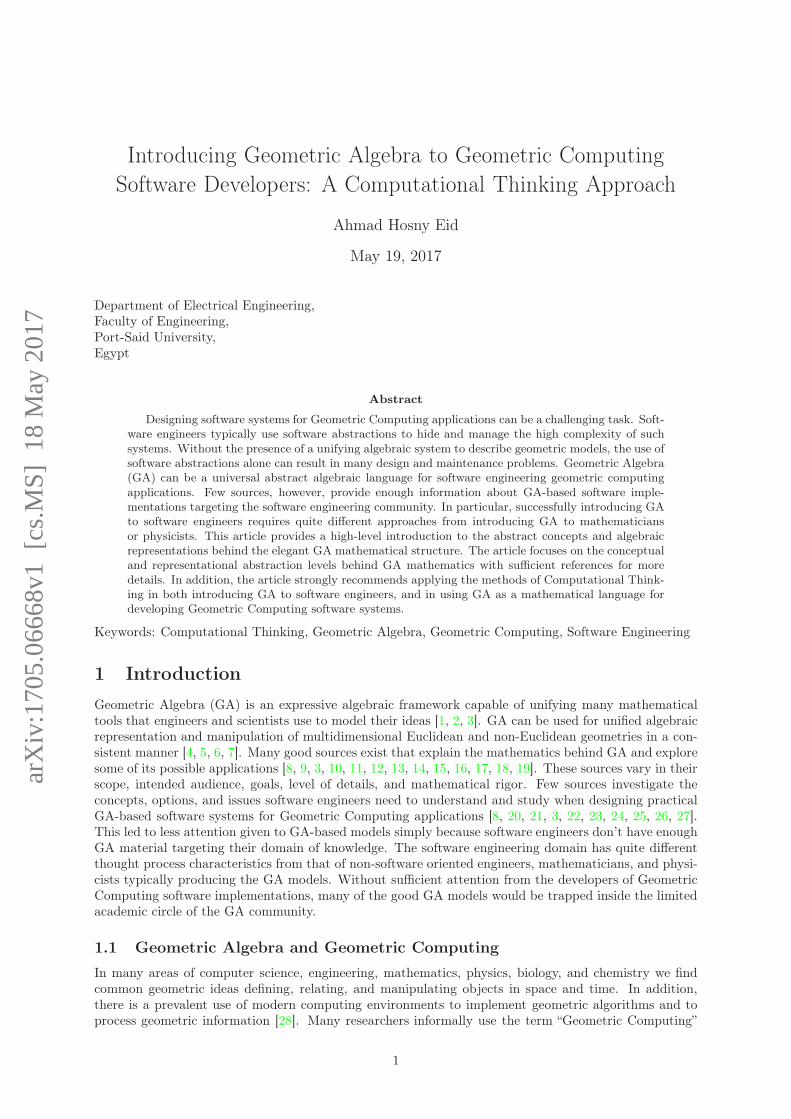
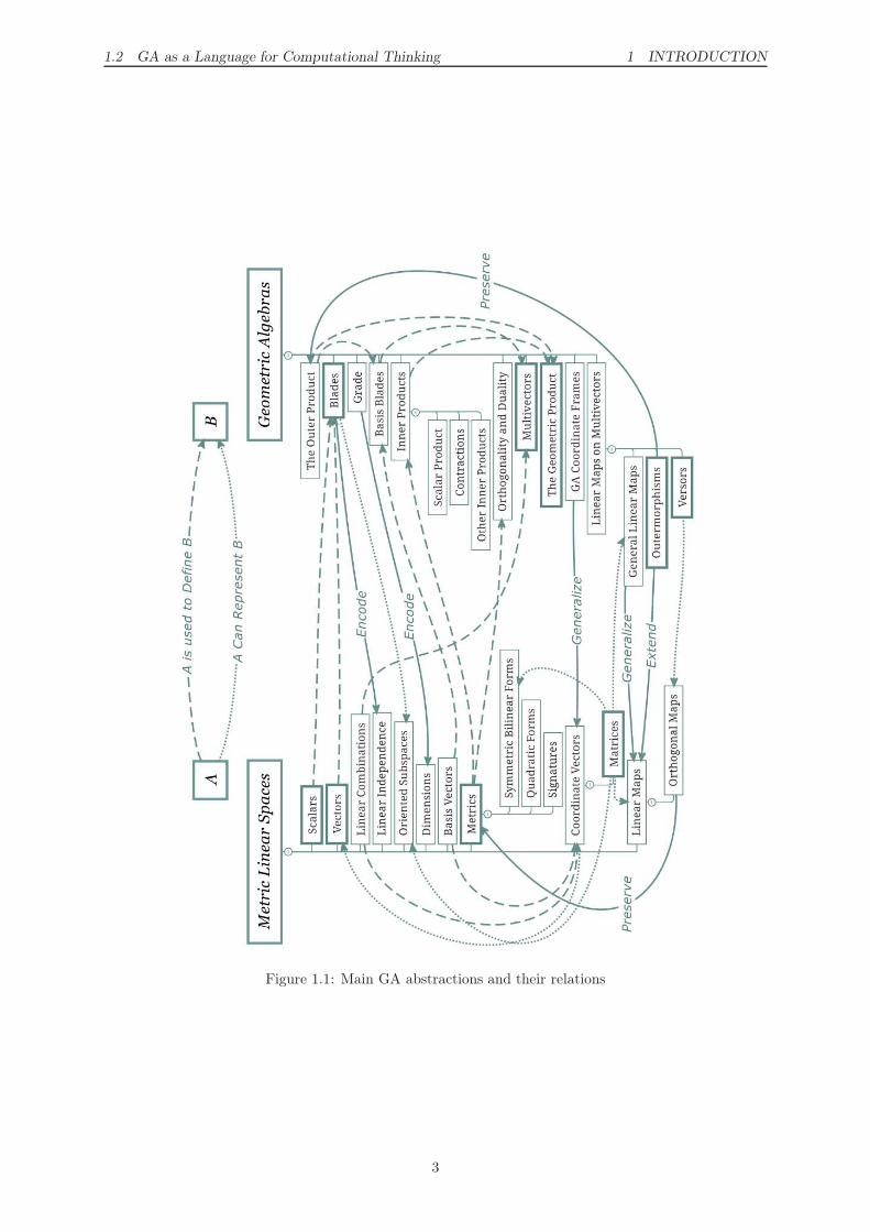
Figure 1.1: Main GA abstractions and their relations

3

1.2 GA as a Language for Computational Thinking 1 INTRODUCTION

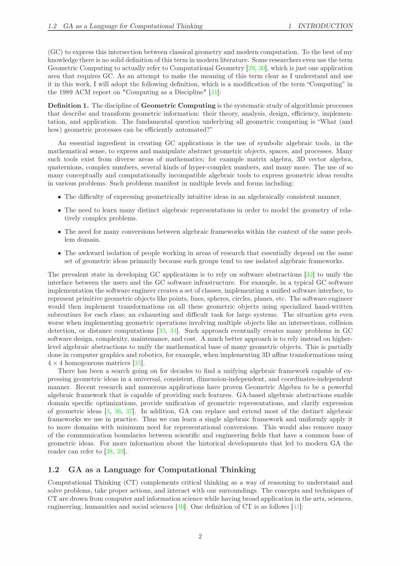
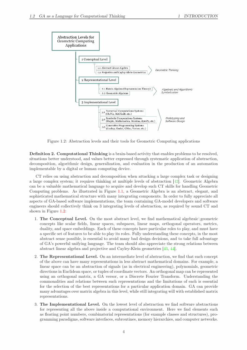
Figure 1.2: Abstraction levels and their tools for Geometric Computing applications

Definition 2. Computational Thinking is a brain-based activity that enables problems to be resolved,situations better understood, and values better expressed through systematic application of abstraction,decomposition, algorithmic design, generalization, and evaluation in the production of an automationimplementable by a digital or human computing device.

CT relies on using abstraction and decomposition when attacking a large complex task or designinga large complex system; it requires thinking at multiple levels of abstraction [42]. Geometric Algebracan be a valuable mathematical language to acquire and develop such CT skills for handling GeometricComputing problems. As illustrated in Figure 1.1, a Geometric Algebra is an abstract, elegant, andsophisticated mathematical structure with many integrating components. In order to fully appreciate allaspects of GA-based software implementations, the team containing GA-model developers and softwareengineers should collectively think on 3 integrating levels of abstraction, as required by sound CT andshown in Figure 1.2:

1. The Conceptual Level. On the most abstract level, we find mathematical algebraic\geometricconcepts like scalar fields, linear spaces, subspaces, linear maps, orthogonal operators, metrics,duality, and space embeddings. Each of these concepts have particular roles to play, and must havea specific set of features to be able to play its roles. Fully understanding these concepts, in the mostabstract sense possible, is essential to avoid many bad design decisions, and to take full advantageof GA’s powerful unifying language. The team should also appreciate the strong relations betweenabstract linear algebra and projective and Cayley-Klein geometries [43, 44].

2. The Representational Level. On an intermediate level of abstraction, we find that each conceptof the above can have many representations in less abstract mathematical domains. For example, alinear space can be an abstraction of signals (as in electrical engineering), polynomials, geometricdirections in Euclidean space, or tuples of coordinate vectors. An orthogonal map can be representedusing an orthogonal matrix, a GA versor, or a Discrete Fourier Transform. Understanding thecommonalities and relations between such representations and the limitations of each is essentialfor the selection of the best representations for a particular application domain. GA can providemany advantages over matrix algebra in this level, while still integrating will with established matrixrepresentations.

3. The Implementational Level. On the lowest level of abstraction we find software abstractionsfor representing all the above inside a computational environment. Here we find elements suchas floating point numbers, combinatorial representations (for example classes and structures), pro-gramming paradigms, software interfaces, subroutines, memory hierarchies, and computer networks.

4

1.2 GA as a Language for Computational Thinking 1 INTRODUCTION

Computers impose many physical constraints on the above two levels of abstraction that must betaken into consideration when addressing practical GA-based software implementations. Many GA-based software tools are currently present to be used at this level including numerical, symbolic,and Generative Programming-based systems.

These three levels are familiar to software engineers in other domains of application. For example, indatabase systems design we find three analogous levels of Conceptual Design, Logical Design, and PhysicalDesign [45]. The role GA plays in Geometric Computing applications can be thought to be analogousto the role of Relational Algebra in relational database systems design. The study of the mathematicsbehind Relational Algebra alone is not sufficient to produce successful database applications, however.Software engineers must address other complementary aspect of the design related to user interactionwith data (using SQL as a Domain Specific Language for example), physical storage and transfer of data,optimization of data query executions, data visualization and presentation, scalability, and many more.Without addressing such aspects, Relational Algebra wouldn’t have become a basic part of computerscience curricula worldwide. We must address similar complementary aspects for Geometric Algebra inorder to achieve its rightful place in the scientific, educational, and industrial fields.

Whenever possible, expressing our ideas at the top level of abstraction is very powerful conceptually.At this level we can understand and relate many application areas at a fundamental level. We cancommunicate ideas and transfer knowledge between them more easily. Sadly, many people don’t haveaccess to this level of abstraction in practice. We are taught to think about our mathematical tools startingfrom the second intermediate level of abstraction, not the first top level. The benefits of eliminating thisserious problem appears in all areas in which GA can be applied; for example:

• Many transformations we apply in signal and image processing are just instances of abstract orthog-onal linear maps, with more unifying common properties than initially perceived. Such transformsinclude continuous and discrete Fourier transforms, Laplace, z-, Walsh-Hadamard, slant, Haar,Karhunen-Loeve, and wavelet transforms [46]. Using GA to represent and apply these transformscan lead to new applications and insights [47, 48], and eventually to new unified architectures formulti-dimensional signal processing software systems with modeling and processing capabilities wellbeyond the current systems.

• In geometric modeling and geometric reasoning, Euclidean, Hyperbolic, and Elliptic geometrieshave a common algebraic foundation within GA. This enables us to create GA-based universalgeometric constructions and apply them to specific problems with any desired geometry of thesethree [4, 5, 6, 7]. Some dynamic geometry software systems already apply this approach, likeCinderella [49, 50] that internally models the general Cayley-Klein geometry using complex numbers[44].

• Many algebras that are very useful in practice are actually sub-algebras of some GA. The listinclude the algebra of real numbers, complex numbers, n-D Euclidean vectors, quaternions, dualquaternions, spinors, Clifford’s dual numbers, and Grassmann numbers. GA can unify and convertthese numbers within the context of a single problem, engineering discipline, or scientific field.

Another anti-CT pattern facing most software engineers in designing GC applications results from nothaving a clear separation between those three levels of abstraction. In many cases, intermediate repre-sentational abstractions are incorrectly perceived to be identical to the conceptual abstractions. As anexample, consider the default use of matrices to represent linear maps in GC applications. There areother intermediate representations that are better than matrices in modeling certain geometric aspectswith better computational properties. For example, it’s much easier to extract the axis and angle of rota-tion of a 3D general rotation linear map if we use a quaternion to represent the linear map. Quaternionsrequire less memory, less processing, and are numerically more stable compared to rotation matrices [3].As another example for incorrectly mixing levels of abstraction, many programmers blindly use floatingpoint numbers as a perfect representation of real numbers, not taking into consideration some of theirproblematic features [51].

Clear separation of the first two abstraction levels can result from studying a course in projectivegeometry [44], abstract algebra [52], and abstract linear spaces [53, 54] in addition to the classical co-ordinate based linear algebra courses [55]. GA can be very helpful in this regard as it contains enoughmathematical abstraction and generality to provide clear understanding and separation of abstract levelsof thinking. This skill is typically available to mathematicians and physicists, but less so for computerscientists and engineers. Separation of the third level requires careful study of the physical limitations of

5

1.3 Aims and Contents 2 METRIC LINEAR SPACES

representing and communicating information inside computational environments. In addition, a throughunderstanding of capabilities of modern programming languages and programming paradigms is neces-sary to design better implementations [56, 57]. This skill is typically available to computer scientists andsoftware engineers, but less so for mathematicians and physicists.

From another angle, learning GA can take much time and effort. Applying Computational Thinkingto the GA learning problem can reduce time and effort considerably. Because GA is relevant to so manyareas in science and engineering, its presentation should be formulated to each specific discipline. Avery good example for presenting GA to electrical and electronic engineers, for example, is [17]. Similarefforts are needed to properly introduce GA to software engineers and software developers. PresentingGA to a software engineer is different from presenting to a mathematician or physicist. The mindset ofa software engineer prefers dealing with diagrams, specifications, relations, and algorithms rather thanaxioms, theorems, proofs, and equations [8]. Such efforts also include designing easy to use domain-specific GA-based software systems for educational and prototyping purposes in addition to productionpurposes for Geometric Computing applications.

1.3 Aims and Contents

This article is intended as a Computational Thinking driven exposition of GA for software engineersinterested in creating GA-based GC software systems. I attempt to emphasize the conceptual and rep-resentational abstraction levels related to each mathematical element of Geometric Algebra, leaving theimplementational level to future articles. The conceptual level is purely mathematical and is independentof any particular software implementation. The representational level is also mathematical but typicallydefines the high-level design of the GA-based software system. My main intention here is to provide aunified entry point for facilitating further study of the mathematics behind the concepts summarized herethat is suitable for software engineers.

The main body of this article consists of 3 parts. In the first part of this article in section 2, Isummarize the main abstract and algebraic concepts of Metric Linear Spaces, the base on which GAs areconstructed. In the second part in section 3, I build on the concepts of section 2 to explain the elegantmathematical structure of Geometric Algebra with references to additional information sources for theinterested reader. Since I’m mainly interested here in the most computationally-significant algebraicconstructions of GA, I will not discuss GA’s numerous geometric interpretations found in the literature.In the third part in section 4, I focus on defining GA Coordinate Frames and how to use them forcomputing linear operations, products, and maps on GA multivectors. This is the mathematical base forthe symbolic computations infrastructure layer in GMac, a universal GA-based implementation generatorsystem I designed [58, 59]. Finally, in section 5 I provide some concluding remarks and suggestions.

2 Metric Linear Spaces

2.1 Scalar Fields

Many number systems exist in mathematics with varying properties and applications. In practice, how-ever, we tend to concentrate on a few of them: rational numbers Q , real numbers R , and complexnumbers C . Such numbers are also called scalars to distinguish them from vectors in linear spaces.There are common properties of these number systems that, when abstracted into algebraic relations,give us the concept of a scalar field [52]. On the top conceptual level of abstraction, a field F is a set of“scalars” closed under two operations called addition and multiplications satisfying some familiar prop-erties like associativity and commutativity of addition and multiplication, presence of unique additiveand multiplicative identities and inverses, and distributivity of multiplication over addition. From thesesimple properties many features, theorems, and operations can be defined and deduced based on theseabstract concepts without having to give concrete examples like the real or complex number systems.Some roles of scalars in Geometric Computing applications include:

• Used as abstractions of physical measurements like mass, velocity, length, area, etc..

• Used to encode, quantify, sort, and compare geometric objects and their properties.

• Used as construction elements in Linear Combinations and other related combinations over Vectors.

Mathematically, we can construct a linear space, hence a GA, over any scalar field; including finite fields[60]. Linear spaces over finite fields have interesting properties that could be investigated using Geometric

6

2.2 Linear Combinations and Abstract Vectors 2 METRIC LINEAR SPACES

Algebra especially for digital and discrete geometry applications [61, 62]. In the GA literature there existstrong assertions that only real numbers should be used as a base for constructing GAs [39]. This pointof view is mainly based on the existence of isomorphisms between complex numbers-based GAs and realnumbers-based GAs; so the use of complex-based GAs is mathematically redundant and geometricallymore complex for modeling the physical space and time we live in. This is certainly a respectable pointof view, especially in physics. From a software engineering and educational point of view, however, Irecommend to leave the door open for using the most suitable number system for a particular problemat hand. I believe many problems can be more easily transformed from the classical representations intoGA-based representations if we are flexible about the choice of the number system we use [11].

2.2 Linear Combinations and Abstract Vectors

At the base of the elegant GA mathematical structure we find the abstract concept of Linear Spaces;also commonly called Vector Spaces [53, 54, 55]. Many study linear spaces because of their basic rolein encoding the Superposition Principle; a cornerstone in modern science and engineering. Typicalmathematical introductions to linear spaces concentrate on the abstract algebraic properties of vectorsand their two main operations of vector addition and scalar multiplication. From a computational pointof view, however, the central concept in linear spaces is the Linear Combination. A linear combination isan expression of the form a1v1 + a2v2 + · · ·+ akvk ≡

∑ki=1 aivi where vi are “vectors” and ai are scalars

not all zero. A linear space is simply any set of “vectors” that is closed under linear combinations over agiven scalar field; i.e. any linear combination of any collection of vectors is also a vector in the same set.The familiar algebraic properties of vector addition and scalar multiplication are necessary to performlinear combinations consistently. This very abstract concept has so many manifestations in science andengineering that it is a central concept in many applications. All other main concepts of linear spacesare derived from linear combinations; for example:

• Span: The span of a given set of vectors span (v1, v2, . . . , vk) is the set of vectors resulting from allpossible linear combinations of these vectors. Here the vectors vi are fixed while the scalars ai cantake any possible values from their field.

• Subspace: A linear subspace W of a larger linear space V , denoted here as W ≤ V , is a subsetof the linear space V that is closed under linear combinations. The span of any set of vectors fromV is always a subspace of V .

• Linear Independence: A collection of vectors are called Linearly Dependent when we can expressany of them as a linear combination of the others; else they are Linearly Independent (LID) vectors.These two are basic conceptual relations among any given collection of vectors.

• Basis: A basis is a LID set of vectors {e1, e2, . . . , en} that spans the whole linear space. Anyvector in the linear space can be expressed as a unique linear combination of the basis vectors.A linear space can have an infinite number of basis sets, but they all contain the same numberof vectors n. This number n is the dimension of the linear space denoted by dim (V ). In all thefollowing discussions, the basis is assumed to be an ordered set, not a general set; denoted here as〈e1, e2, . . . , en〉.

• Coordinate Vector: Given a fixed ordered basis E = 〈e1, e2, . . . , en〉 we can express any abstractvector v as a linear combination of the basis vectors v =

∑ki=1 aiei. The scalar coefficients ai ∈ F can

be written as a tuple vE = (a1, a2, . . . , an) ∈ Fn that is called the coordinate vector representationof v;. The abstract vector v and its coordinate vector vE are two conceptually distinct entities, buthave a linear isomorphism between them; so we can compute with coordinate vectors and interpretthe results in the context of the abstract linear space. Sometimes we prefer to express the coordinatevector in matrix form as a column vector holding the same scalars. I will denote the column vectorrepresentation of an abstract vector v on the basis E as: [v]E =

[a1 a2 · · · an

]T.

• Linear Map: A linear map is a map between two linear spaces f : V → W that preserves linearcombinations f [

∑ki=1 aivi] =

∑ki=1 aif [vi]. When the two linear spaces are the same, its is called a

linear operator.

• Other Combinations: Imposing constraints on the scalar coefficients of linear combinations leadsto theoretically and practically significant concepts with many important geometric interpretations

7

2.3 Abstract Vectors and Coordinate Vectors 2 METRIC LINEAR SPACES

like Affine Combinations∑k

i=1 ai = 1 [35], Conical Combinations ai ≥ 0, and Convex Combinationsai ≥ 0,

∑ki=1 ai = 1 [63].

It is important to note that we are not yet talking about distances and angles between vectors or or-thogonality of vectors because such concepts require the more fundamental concept of metric definedlater. The main relation between vectors in non-metric abstract linear spaces is the Linear Depen-dence\Independence relation. The main construction operation is the Linear Combination. We can“divide” two vectors (i.e. compare their relative scale) but only if one of them is a linear combination (i.e.a scaled version) of the other. Generally, this is not how engineers are usually taught linear spaces inundergraduate courses, but a clear understanding and separation of these fundamental concepts is nec-essary to correctly understand and use the mathematical structure of Geometric Algebra that is basedon abstract linear spaces.

2.3 Abstract Vectors and Coordinate Vectors

In order to use computers for dealing with abstract concepts of linear spaces, we need an equivalentintermediate representation that only uses numbers and their basic operations of addition and multipli-cation. Mathematics provide a base for such representation through coordinate vectors. Without lossof generality I will concentrate on the field of real numbers R as the scalar field for all the followingdiscussions. Having an n-dimensional abstract linear space V on R with basis E = 〈e1, e2, . . . , en〉 we canset up a linear isomorphism (i.e. one-to-one linear map) φ defined with its inverse map φ−1 as follows:

φ : Rn → V, φ : (a1, a2, . . . , an) 7→n∑

i=1

aiei; (2.1)

φ−1 : V → Rn, φ−1 : v 7→ vE (2.2)

This way, linear combinations on the coordinate vectors of the real linear space Rn are equivalentrepresentations of the same linear combinations on the abstract linear space V . Now we can add twovectors in V by simply adding the real components of their coordinate vectors in Rn and apply the linearisomorphism to get the final result in V . We can do the same for scalar multiplication by multiplying thescalar with the components of the coordinate vector. All derived linear operations on V can be formulated“numerically” on the equivalent real linear space Rn. This is the playground of matrix algebra [55], thetypical starting point where most engineers learn about linear spaces. The n-dimensional real coordinatevectors space Rn is a linear space that is equivalent to all n-dimensional abstract linear spaces; Rn is auniversal intermediate representation for all abstract linear spaces.

One important point to realize is that by changing the basis of V we are also changing the linear iso-morphism φ because the same abstract vector has a different linear combination on a different basis. Tomake our computations consistent we must use the same basis for all related computations. In addition,some facts should remain the same regardless of the used basis and isomorphism. For example, linearindependence of a set of vectors should remain the same regardless of the selected basis. Such propertiesare called coordinate-independent or basis-independent. GA can provide many coordinate-independentformulations for properties of linear spaces and at the same time act as an excellent intermediate rep-resentation through its multivectors and products. Because a GA is itself a linear space, as will beexplained later, we can always represent all GA multivectors and operations using matrix algebra. Thisis the approach used in some GA software systems like the Clifford Multivector Toolbox for MATLAB[64, 65] for example.

2.4 Metrics and Their Representations

A metric linear space is just a linear space with an additional bilinear map, called the metric, thatassociates a scalar with each pair of vectors [66]. The objective of defining a metric is to enable comparingvectors and subspaces of different attitude in space using scalars. Many familiar concepts we use areactually based on the more fundamental metric concept. Such concepts include distance, length, area,angle, orthogonality, orthogonal maps, projections, rotations, and many others. In GA the definition ofa metric is based on the concept of a symmetric bilinear form and the associated concept of a quadraticform. A symmetric bilinear form B on the real linear space V is a mapping B : V × V → R that islinear in both arguments (i.e. bilinear) and symmetric B(u, v) = B(v, u) ∀u, v ∈ V . A related concept

8

2.5 Linear Maps and Their Representations 2 METRIC LINEAR SPACES

is the quadratic form that is related to a symmetric bilinear form by: Q(u) = 12B(u, u), B(u, v) =

Q(u+v)−Q(u)−Q(v) ∀u, v ∈ V . The quadratic form satisfies the relation Q(av) = a2Q(v) ∀v ∈ V, a ∈ R.The metric also associates each vector in the linear space with some scalar by putting the vector in

both inputs of the metric. This scalar is called the norm ‖v‖ ≡ v2 ≡ B(v, v) of the vector v ∈ V andis equal to double the quadratic form of the vector ‖v‖ = 2Q (v)1. If two vectors are associated withthe same scalar they are of equal norm, and null vectors are vectors having zero norm. In this contextthe norm is any general real number; even zero and negative numbers are allowed for non-zero vectorsin GA. This is one important generalization different from metrics in classical linear algebra that areusually restricted to being positive definite. One of the common interpretations of vector norm in thespecial case of Euclidean linear spaces is the the squared length of a direction vector.

If the linear space has the basis 〈e1, e2, · · · , en〉 then we can construct a bilinear form matrix AB =[aij ] , aij = B(ei, ej) , also called the metric matrix on this basis. This matrix is a real symmetric matrixthat we can use to compute the bilinear form of any two vectors u, v ∈ V given their representation onthe basis as follows:

u = u1e1 + · · ·+ unen,

v = v1e1 + · · ·+ vnen

⇒ B(u, v) =(u1 · · · un

)AB

(v1 · · · vn

)T(2.3)

Using bilinear forms the concept of orthogonality of vectors can be defined as follows: two vectorsu, v are called orthogonal iff B(u, v) = 0. The inner product of two vectors is simply the bilinear formof the vectors u · v ≡ B(u, v), and the norm is the inner product of a vector with itself v2 = v · v; thusjustifying the use of the name Inner Product Matrix (IPM) for the symmetric bilinear form matrix. TheIPM AB, being a real symmetric matrix, can be diagonalized using a Change of Basis Matrix (CBM) P

to obtain a diagonal matrix D = PTABP where P is an orthogonal matrix P−1 = PT . The columnsof P are orthogonal eigen vectors for AB. The diagonalization can always be performed such that thenumbers on the diagonal (called the eigen values) are either -1, 0, or +1. The number of eigen valuesthat are 1,-1, and 0 are characteristics for a given metric and define what is called the signature of thebilinear\quadratic form. A bilinear\quadratic form is said to have the signature (p, q, r) if there exists adiagonalization of the IPM having p eigen values with value 1, q eigen values with value -1 and r eigenvalues with value zero. If the IPM is singular (i.e. has no inverse which is equivalent to r > 0) the bilinearform is called degenerate. If all the eigen values are positive the IPM is positive definite and the spaceis a Euclidean space; there exists a basis with all basis vectors norms equal to +1. A mixed-signaturemetric space has some non-zero vectors with norm equal to zero. Such vectors are called null vectors andonly exist in mixed-signature spaces (spaces having a bilinear form with p > 0 and q > 0) in addition todegenerate spaces. The signature of the IPM extends to the signature of the whole GA that we constructusing the IPM. By combining the concept of metric and the concept of space embedding, discussed later,we can consistently model Euclidean and non-Euclidean geometries using GAs of various signatures.

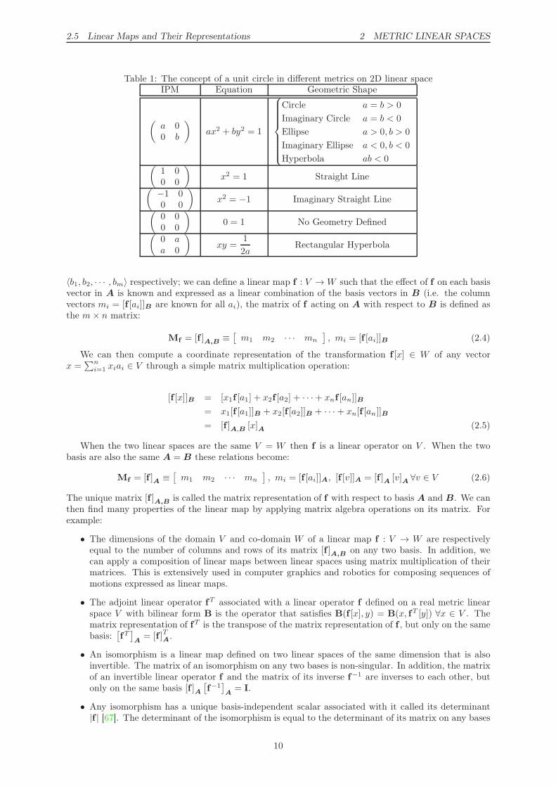
To illustrate how a metric effects the geometry of the space, Table 1 shows some possible metricsof a 2D linear space with basis 〈e1, e2〉. Using this general definition of the unit circle “The set ofposition vectors having unit norm {v : v = xe1 + ye2, ‖v‖ = 1, x, y ∈ R}” we get the general equationx2e21 + 2xy (e1 · e2) + y2e22 = 1. We see that only in Euclidean space ei · ej = δ

ji where we get the

familiar circle equation, where in other metrics we get totally different geometries. The same goes forthe geometric meanings of other metric-dependent concepts like orthogonality, angle, rotation, distance,area, projection, etc.

2.5 Linear Maps and Their Representations

Linear maps are a central concept for creating Geometric Computing applications. One of the mainreasons is that linear maps have a direct relation to multi-dimensional Projective Geometry [44, 36],which is the base for all Euclidean and non-Euclidean geometries, and has many applications in computergraphics, computer vision, robotics, and image processing, for example. I will denote the effect of a linearmap f : V → W on a vector x ∈ V and on a subspace X = span (x1, x2, . . . xk) ≤ V as f [x] ∈ W andf [X ] ≤W respectively. Classically the concept of a linear map is associated with matrix algebra throughthe following construction: assuming the real linear spaces V,W with bases A = 〈a1, a2, · · · , an〉 ,B =

1This is different from classical literature where the norm of a Euclidean vectors x is the square root of the inner product√x · x equivalent to its length. I will use here the notation |x| = √

x · x assuming x · x ≥ 0.

9

2.5 Linear Maps and Their Representations 2 METRIC LINEAR SPACES

Table 1: The concept of a unit circle in different metrics on 2D linear spaceIPM Equation Geometric Shape

(a 00 b

)ax2 + by2 = 1

Circle a = b > 0

Imaginary Circle a = b < 0

Ellipse a > 0, b > 0

Imaginary Ellipse a < 0, b < 0

Hyperbola ab < 0(1 00 0

)x2 = 1 Straight Line

(−1 00 0

)x2 = −1 Imaginary Straight Line

(0 00 0

)0 = 1 No Geometry Defined

(0 a

a 0

)xy =

1

2aRectangular Hyperbola

〈b1, b2, · · · , bm〉 respectively; we can define a linear map f : V →W such that the effect of f on each basisvector in A is known and expressed as a linear combination of the basis vectors in B (i.e. the columnvectors mi = [f [ai]]B are known for all ai), the matrix of f acting on A with respect to B is defined asthe m× n matrix:

Mf = [f ]A,B ≡[m1 m2 · · · mn

], mi = [f [ai]]B (2.4)

We can then compute a coordinate representation of the transformation f [x] ∈ W of any vectorx =

∑ni=1 xiai ∈ V through a simple matrix multiplication operation:

[f [x]]B = [x1f [a1] + x2f [a2] + · · ·+ xnf [an]]B

= x1[f [a1]]B + x2[f [a2]]B + · · ·+ xn[f [an]]B

= [f ]A,B [x]A (2.5)

When the two linear spaces are the same V = W then f is a linear operator on V . When the twobasis are also the same A = B these relations become:

Mf = [f ]A ≡[m1 m2 · · · mn

], mi = [f [ai]]A, [f [v]]A = [f ]A [v]A ∀v ∈ V (2.6)

The unique matrix [f ]A,B is called the matrix representation of f with respect to basis A and B. We canthen find many properties of the linear map by applying matrix algebra operations on its matrix. Forexample:

• The dimensions of the domain V and co-domain W of a linear map f : V → W are respectivelyequal to the number of columns and rows of its matrix [f ]A,B on any two basis. In addition, wecan apply a composition of linear maps between linear spaces using matrix multiplication of theirmatrices. This is extensively used in computer graphics and robotics for composing sequences ofmotions expressed as linear maps.

• The adjoint linear operator fT associated with a linear operator f defined on a real metric linearspace V with bilinear form B is the operator that satisfies B(f [x], y) = B(x, fT [y]) ∀x ∈ V . Thematrix representation of fT is the transpose of the matrix representation of f , but only on the samebasis:

[fT]A

= [f ]TA.

• An isomorphism is a linear map defined on two linear spaces of the same dimension that is alsoinvertible. The matrix of an isomorphism on any two bases is non-singular. In addition, the matrixof an invertible linear operator f and the matrix of its inverse f−1 are inverses to each other, butonly on the same basis [f ]A

[f−1]A

= I.

• Any isomorphism has a unique basis-independent scalar associated with it called its determinant|f | [67]. The determinant of the isomorphism is equal to the determinant of its matrix on any bases

10

2.6 Oriented Subspaces 2 METRIC LINEAR SPACES

|f | =∣∣∣[f ]A,B

∣∣∣. The geometric significance of the determinant is more apparent within the context

of GA’s outermorphisms discussed later.

• We can define a unique Change of Basis isomorphism between two linear spaces of the same dimen-sion g : V → W that takes A to B such that g [ai] = bi ∀i = 1, 2, . . . , n.. This isomorphism alsohas a unique invertible matrix [g]A,B called a Change of Basis Matrix (CBM). This means that thesame invertible matrix may represent an invertible linear operator on the same basis, or a changeof basis linear map on two different bases. This is one instance of mixing of conceptual abstractionsthat is common in matrix algebra formulations. Such issue might lead to confusions in algebraicformulations when using matrix algebra to represent abstract linear maps.

• Two matrices M ,N are called similar M ∼N if they represent the same linear operator on differentbases, or equivalently if there is a CBM C such that M = C−1

NC. Similarity between squarematrices is an equivalence relation. Many invariant properties of similar matrices are actuallyproperties of their common abstract linear map. Most notably, spectral analysis and invariantsubspace techniques in linear algebra [68] depend on this relation between an abstract linear mapand its infinite number of representation matrices. These techniques are very important in manyscientific and engineering applications.

• An invertible linear operator f that satisfies B(f [x], f [y]) = B(x, y) ∀x, y ∈ V , where B is the bilinearform on V , is called an orthogonal linear operator; it preserves the metric between vectors. Thismeans that f preserves many metric-dependent properties and operations like the inner product,norm, orthogonality, and angle between vectors. In addition, its adjoint is equal to its inverse:f−1 = f . For non-degenerate metrics, the matrix of an orthogonal operator is invertible, has ±1determinant, and has columns that represent orthonormal vectors; i.e. each two column vectorsare orthogonal and have unit (i.e. ±1) norm. These matrices are called orthogonal matrices andare very important in many practical applications. We can analyze\construct any such map as acomposition of a series of geometric reflections in homogeneous hyper-planes (i.e. (n−1)-dimensionalsubspaces) of the linear space. The Householder operator [69, 70, 71], one of the most importantcomputational tools in numerical matrix algebra, is based on this conceptual construction. GAprovide a better algebraic alternative using its Versors and Versor Product.

• The Kernel kerf or Null Space of a linear map f : V →W is the set of vectors that transform to thezero vector of W under f : kerf = {v : v ∈ V, f [v] = 0W }. The range rangef or Image of f is the setof vectors in W that are transformations under f of vectors in V : rangef = {w : ∃v ∈ V f [v] = w}.These two sets are subspaces satisfying the relations kerf ≤ V , rangef ≤ W , and dim (V ) =dim (kerf ) + dim (rangef ) where nullf ≡ dim (kerf ) is also called the nullity off and rankf ≡dim (rangef ) is called the rank off . We can use matrix algebra to find the kernel of f using itsrepresentation matrix [f ]A,B on any two bases by solving the matrix equation [f ]A,B v = 0 forcoordinate vectors v to find a set of LID spanning coordinate vectors for the kernel. We can alsorepresent the range of a linear map using [f ]A,B by viewing its column vectors as representingabstract vectors in W that span rangef . This leads to the familiar matrix rank of [f ]A,B being

equal to the rank of the linear map it represents rank([f ]A,B

)= rankf . These linear spaces and

their relations are an important part of the Fundamental Theorem of Linear Algebra [72] usuallyexpressed using matrices not abstract linear maps.

It is very important when designing Geometric Computing applications in a Computational Thinkingsound manner to have clear conceptual distinction between an abstract linear map and its infinite numberof possible matrix representations. In GC applications it is typical that the choice of basis is not arbitraryor even unique. The same problem may need many bases to be used, as in the case of robotics andcomputer graphics for example. Because matrices can also represent subspaces (as lists of column vectors)and metrics (as IPMs), matrix algebra formulations can hide the abstract geometric meaning behind theclutter of its less abstract and basis-implicit representations. The use of GA formulations instead ofmatrix algebra can, in many cases, enforce a clear separation of basic abstract concepts from theirrepresentations.

2.6 Oriented Subspaces

When we use matrix algebra to represent linear spaces, we have a well-developed set of tools to alge-braically represent and manipulate abstract vectors. In many applications in science and engineering,

11

2.6 Oriented Subspaces 2 METRIC LINEAR SPACES

however, we often need to algebraically represent and manipulate whole subspaces in addition to vectors.Some common subspace manipulations we use include:

• To construct a subspace given a set of vectors that spans the subspace; the vectors may or may notbe linearly independent.

• We may need to extract information about a subspace such as its dimensionality, its relation to fixedsubspaces in the problem, and the “best” basis of vectors we can use to span the subspace. Herethe word “best” is context-dependent. We may prefer a basis for getting more numerically-stablecomputations, or perhaps for having a better correspondence with actual physical elements of ourmodel.

• To apply a linear map to a whole subspace and get another.

• To operate on two or more subspaces in order to get another subspace as output. For example, tofind the common subspace of two subspaces, to find the smallest subspace containing two subspaces,to project one subspace on another, to find a subspace that complements another into a biggersubspace, and to reflect one subspace on another.

• To compare two subspaces having different attitudes in space. This includes, for example, findingthe angle of a single rotation operation that takes one subspace into another, or finding if twosubspaces are orthogonal to each other in the sense that each vector in the first is orthogonal to allvectors in the second subspace.

Any single vector v actually represents a 1-dimentional subspace ←→v through its span: ←→v = span (v).Extending this to more dimensions we can use the span of k LID vectors to represent their k-dimensionalsubspace W = span (v1, v2, . . . , vk). A matrix AW can represent an ordered set of vectors by puttingtheir equivalent coordinate representations on some basis E as rows or columns in the matrix: AW =[[v1]E [v2]E · · · [vk]E

]. This way we can use matrix algebra and matrix operations to manipulate

this “list of coordinate vectors” as an indirect (and mostly awkward) computational representation of ab-stract linear subspaces. This kind of representation has disadvantages for practical Geometric Computingapplications. Matrix algebra is a suitable mathematical abstraction for low-level computations inside ma-chines, but is not an intuitive modeling abstractions when designing GC models and algorithms. Muchgeometric information get scattered among the numbers of the matrix, and we need significant effort toextract such information. In addition, matrix algebra-based formulations are often basis-dependent andmetric-dependent. As I will explain in the next section, Geometric Algebra can provide more powerfuland geometrically significant representations for subspaces using GA’s Blades. GA-based formulationsare found to be significantly more compact and basis-independent for many applications.

While the set intersection U ∩W of two subspaces U,W ≤ V is also a subspace in V , their set unionU ∪ W is not guaranteed to be a linear space. An analogous operation to set union that guaranteesa subspace result is called the sum of subspaces defined as W + U = {x :: x = w + u; w ∈ W,u ∈V }, W, V ≤ V . Having a set of mutually disjoint subspaces W1,W2, · · · ,Wk ≤ V (i.e. Wi ∩ Wj ={0} ∀i, j = 1, 2, · · ·k, i 6= j) the subspace sum of Wi is called the direct sum of the disjoint subspacesand is denoted by ⊕k

i=1Wi ≡W1⊕W2⊕ · · · ⊕Wk. The dimension of the direct sum of disjoint subspacesis equal to the numerical sum of their respective dimensions dim

(⊕k

i=1Wi

)=∑k

i=1 dim (Wi). We oftenuse this notation to construct a larger linear space, like the linear Grassmann space of multivectors, outof a number of mutually disjoint linear spaces. This conceptual construction is metric-independent andbasis-independent.

Another important concept is the orthogonal complement of a metric subspace W ≤ V defined byW⊥ = {x :∈ V : y ⊥ x∀y ∈ W}. The orthogonal complement of a subspace W ≤ V has the followingproperties:

V = W ⊕W⊥ (2.7)

x ⊥ y ∀x ∈W, y ∈W⊥ (2.8)

(W⊥)⊥ = W (2.9)

The classical treatment of subspaces in linear algebra mostly deals with un-oriented subspaces, werea subspace is just a set of vectors closed under linear combinations. In many practical scientific andengineering applications, however, we need to distinguish between two opposite orientations for any

12

2.7 Space Embeddings 2 METRIC LINEAR SPACES

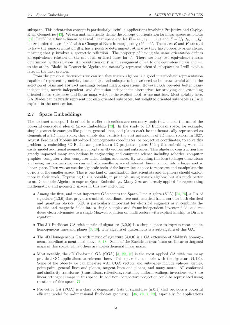
subspace. This orientation concept is particularly useful in applications involving Projective and Cayley-Klein Geometries [43]. We can mathematically define the concept of orientation for linear spaces as follows[67]: Let V be a finite-dimensional real linear space and let E = 〈e1, e2, . . . , en〉 and F = 〈f1, f2, . . . , fn〉be two ordered bases for V with a Change of Basis isomorphism g : V → V . The bases E and F are saidto have the same orientation iff g has a positive determinant; otherwise they have opposite orientations,meaning that g involves a geometric reflection. The property of having the same orientation definesan equivalence relation on the set of all ordered bases for V . There are only two equivalence classesdetermined by this relation. An orientation on V is an assignment of +1 to one equivalence class and −1to the other. Blades in Geometric Algebra can naturally represent oriented subspaces as I will explainlater in the next section.

From the previous discussions we can see that matrix algebra is a good intermediate representationcapable of representing metrics, linear maps, and subspaces; but we need to be extra careful about theselection of basis and abstract meanings behind matrix operations. However, GA provides better basis-independent, metric-independent, and dimension-independent alternatives for studying and extendingoriented linear subspaces and linear maps without the explicit need to use matrices. Most notably here,GA Blades can naturally represent not only oriented subspaces, but weighted oriented subspaces as I willexplain in the next section.

2.7 Space Embeddings

The abstract concepts I described in earlier subsections are necessary tools that enable the use of thepowerful conceptual idea of Space Embedding [73]. In the study of 3D Euclidean space, for example,simple geometric concepts like points, general lines, and planes can’t be mathematically represented aselements of a 3D linear space; they simply don’t satisfy the abstract axioms of 3D linear spaces. In 1827,August Ferdinand Möbius introduced homogeneous coordinates, or projective coordinates, to solve thisproblem by embedding 3D Euclidean space into a 4D projective space. Using this embedding we couldeasily model additional geometric concepts as 4D vectors and subspaces. This algebraic construction hasgreatly impacted many applications in engineering and computer science including robotics, computergraphics, computer vision, computer-aided design, and more. By extending this idea to larger dimensionsand using various metrics, we can embed a smaller space of interest, linear or not, into a larger metriclinear space. Then we can use the algebraic tools of the larger linear space to represent and manipulate theobjects of the smaller space. This is one kind of linearization that scientists and engineers should exploitmore in their work. Expressing this is possible, in principle, using matrix algebra; but it’s much betterto use Geometric Algebra to express Space Embeddings. Many GAs are already applied for representingmathematical and geometric spaces in this way including:

• Among the first, and most important GAs comes the Space-Time Algebra (STA) [74, 75], a GA ofsignature (1,3,0) that provides a unified, coordinate-free mathematical framework for both classicaland quantum physics. STA is particularly important for electrical engineers as it combines theelectric and magnetic fields into a single complex and frame-independent bivector field, and re-duces electrodynamics to a single Maxwell equation on multivectors with explicit kinship to Dirac’sequation.

• The 3D Euclidean GA with metric of signature (3,0,0) is a simple space to express rotations onhomogeneous lines and planes [3, 18]. The algebra of quaternions is a sub-algebra of this GA.

• The 4D Homogeneous GA with metric of signature (4,0,0) is a GA extension of Möbius’s homoge-neous coordinates mentioned above [3, 18]. Some of the Euclidean transforms are linear orthogonalmaps in this space, while others are non-orthogonal linear maps.

• Most notably, the 5D Conformal GA (CGA) [3, 22, 76] is the most applied GA with too manypractical GC applications to reference here. This space has a metric with the signature (4,1,0).Some of the objects we can linearize with CGA vectors and subspaces include spheres, circles,point-pairs, general lines and planes, tangent lines and planes, and many more. All conformaland similarity transforms (translations, reflections, rotations, uniform scalings, inversions, etc.) arelinear orthogonal maps in this space. In addition, perspective projection could be represented usingrotations of this space [77].

• Projective GA (PGA) is a class of degenerate GAs of signatures (n,0,1) that provides a powerfulefficient model for n-dimensional Euclidean geometry. [36, 78, 7, 79], especially for applications

13

3 GEOMETRIC ALGEBRAS

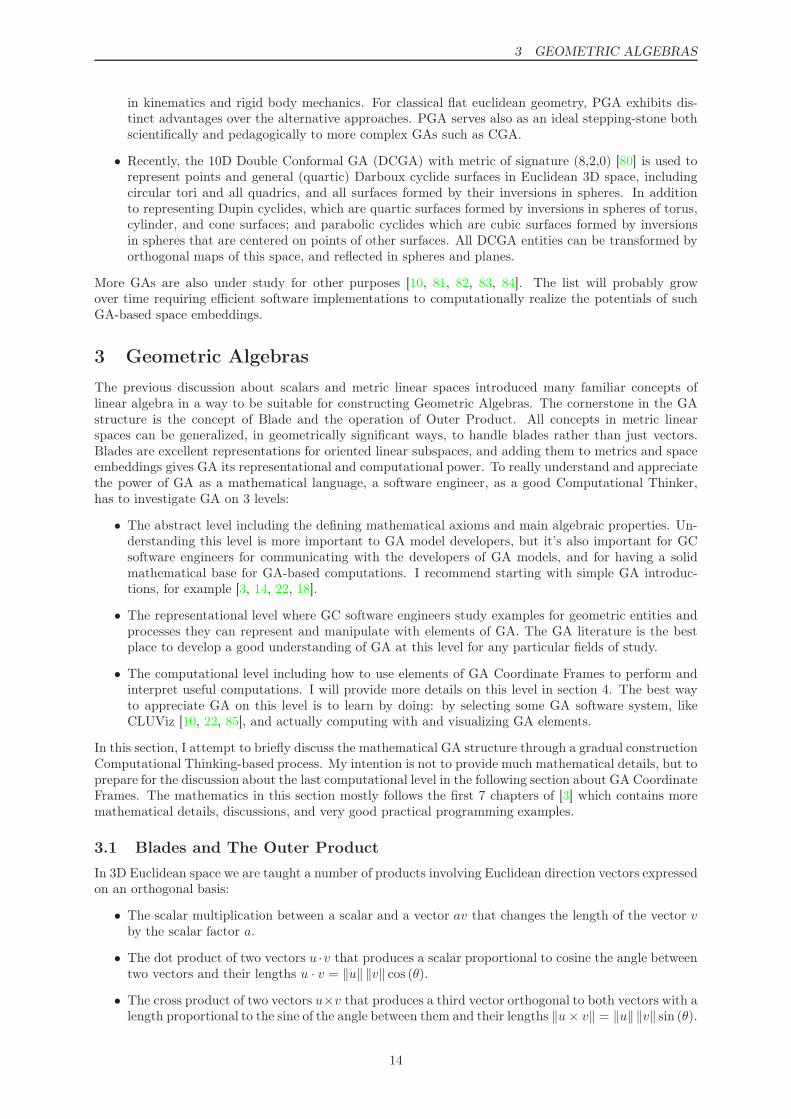
in kinematics and rigid body mechanics. For classical flat euclidean geometry, PGA exhibits dis-tinct advantages over the alternative approaches. PGA serves also as an ideal stepping-stone bothscientifically and pedagogically to more complex GAs such as CGA.

• Recently, the 10D Double Conformal GA (DCGA) with metric of signature (8,2,0) [80] is used torepresent points and general (quartic) Darboux cyclide surfaces in Euclidean 3D space, includingcircular tori and all quadrics, and all surfaces formed by their inversions in spheres. In additionto representing Dupin cyclides, which are quartic surfaces formed by inversions in spheres of torus,cylinder, and cone surfaces; and parabolic cyclides which are cubic surfaces formed by inversionsin spheres that are centered on points of other surfaces. All DCGA entities can be transformed byorthogonal maps of this space, and reflected in spheres and planes.

More GAs are also under study for other purposes [10, 81, 82, 83, 84]. The list will probably growover time requiring efficient software implementations to computationally realize the potentials of suchGA-based space embeddings.

3 Geometric Algebras

The previous discussion about scalars and metric linear spaces introduced many familiar concepts oflinear algebra in a way to be suitable for constructing Geometric Algebras. The cornerstone in the GAstructure is the concept of Blade and the operation of Outer Product. All concepts in metric linearspaces can be generalized, in geometrically significant ways, to handle blades rather than just vectors.Blades are excellent representations for oriented linear subspaces, and adding them to metrics and spaceembeddings gives GA its representational and computational power. To really understand and appreciatethe power of GA as a mathematical language, a software engineer, as a good Computational Thinker,has to investigate GA on 3 levels:

• The abstract level including the defining mathematical axioms and main algebraic properties. Un-derstanding this level is more important to GA model developers, but it’s also important for GCsoftware engineers for communicating with the developers of GA models, and for having a solidmathematical base for GA-based computations. I recommend starting with simple GA introduc-tions, for example [3, 14, 22, 18].

• The representational level where GC software engineers study examples for geometric entities andprocesses they can represent and manipulate with elements of GA. The GA literature is the bestplace to develop a good understanding of GA at this level for any particular fields of study.

• The computational level including how to use elements of GA Coordinate Frames to perform andinterpret useful computations. I will provide more details on this level in section 4. The best wayto appreciate GA on this level is to learn by doing: by selecting some GA software system, likeCLUViz [10, 22, 85], and actually computing with and visualizing GA elements.

In this section, I attempt to briefly discuss the mathematical GA structure through a gradual constructionComputational Thinking-based process. My intention is not to provide much mathematical details, but toprepare for the discussion about the last computational level in the following section about GA CoordinateFrames. The mathematics in this section mostly follows the first 7 chapters of [3] which contains moremathematical details, discussions, and very good practical programming examples.

3.1 Blades and The Outer Product

In 3D Euclidean space we are taught a number of products involving Euclidean direction vectors expressedon an orthogonal basis:

• The scalar multiplication between a scalar and a vector av that changes the length of the vector v

by the scalar factor a.

• The dot product of two vectors u ·v that produces a scalar proportional to cosine the angle betweentwo vectors and their lengths u · v = ‖u‖ ‖v‖ cos (θ).

• The cross product of two vectors u×v that produces a third vector orthogonal to both vectors with alength proportional to the sine of the angle between them and their lengths ‖u× v‖ = ‖u‖ ‖v‖ sin (θ).

14

3.1 Blades and The Outer Product 3 GEOMETRIC ALGEBRAS

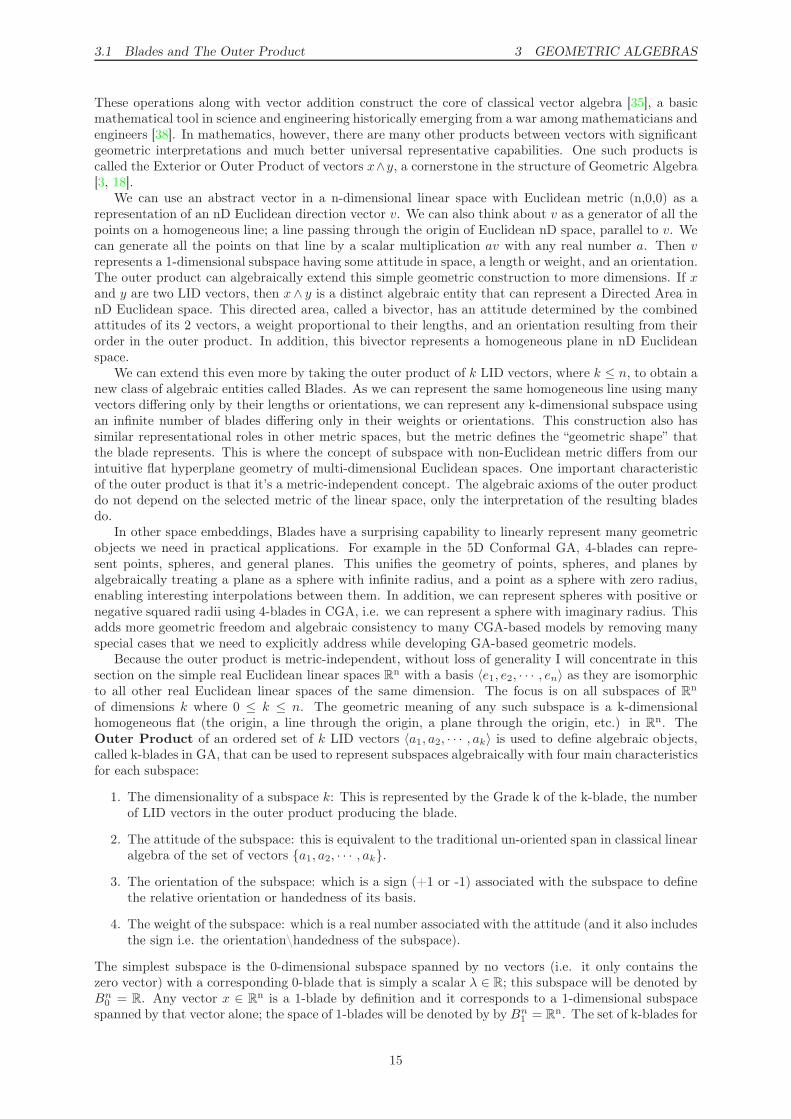
These operations along with vector addition construct the core of classical vector algebra [35], a basicmathematical tool in science and engineering historically emerging from a war among mathematicians andengineers [38]. In mathematics, however, there are many other products between vectors with significantgeometric interpretations and much better universal representative capabilities. One such products iscalled the Exterior or Outer Product of vectors x∧y, a cornerstone in the structure of Geometric Algebra[3, 18].

We can use an abstract vector in a n-dimensional linear space with Euclidean metric (n,0,0) as arepresentation of an nD Euclidean direction vector v. We can also think about v as a generator of all thepoints on a homogeneous line; a line passing through the origin of Euclidean nD space, parallel to v. Wecan generate all the points on that line by a scalar multiplication av with any real number a. Then v

represents a 1-dimensional subspace having some attitude in space, a length or weight, and an orientation.The outer product can algebraically extend this simple geometric construction to more dimensions. If xand y are two LID vectors, then x∧ y is a distinct algebraic entity that can represent a Directed Area innD Euclidean space. This directed area, called a bivector, has an attitude determined by the combinedattitudes of its 2 vectors, a weight proportional to their lengths, and an orientation resulting from theirorder in the outer product. In addition, this bivector represents a homogeneous plane in nD Euclideanspace.

We can extend this even more by taking the outer product of k LID vectors, where k ≤ n, to obtain anew class of algebraic entities called Blades. As we can represent the same homogeneous line using manyvectors differing only by their lengths or orientations, we can represent any k-dimensional subspace usingan infinite number of blades differing only in their weights or orientations. This construction also hassimilar representational roles in other metric spaces, but the metric defines the “geometric shape” thatthe blade represents. This is where the concept of subspace with non-Euclidean metric differs from ourintuitive flat hyperplane geometry of multi-dimensional Euclidean spaces. One important characteristicof the outer product is that it’s a metric-independent concept. The algebraic axioms of the outer productdo not depend on the selected metric of the linear space, only the interpretation of the resulting bladesdo.

In other space embeddings, Blades have a surprising capability to linearly represent many geometricobjects we need in practical applications. For example in the 5D Conformal GA, 4-blades can repre-sent points, spheres, and general planes. This unifies the geometry of points, spheres, and planes byalgebraically treating a plane as a sphere with infinite radius, and a point as a sphere with zero radius,enabling interesting interpolations between them. In addition, we can represent spheres with positive ornegative squared radii using 4-blades in CGA, i.e. we can represent a sphere with imaginary radius. Thisadds more geometric freedom and algebraic consistency to many CGA-based models by removing manyspecial cases that we need to explicitly address while developing GA-based geometric models.

Because the outer product is metric-independent, without loss of generality I will concentrate in thissection on the simple real Euclidean linear spaces Rn with a basis 〈e1, e2, · · · , en〉 as they are isomorphicto all other real Euclidean linear spaces of the same dimension. The focus is on all subspaces of Rn

of dimensions k where 0 ≤ k ≤ n. The geometric meaning of any such subspace is a k-dimensionalhomogeneous flat (the origin, a line through the origin, a plane through the origin, etc.) in Rn. TheOuter Product of an ordered set of k LID vectors 〈a1, a2, · · · , ak〉 is used to define algebraic objects,called k-blades in GA, that can be used to represent subspaces algebraically with four main characteristicsfor each subspace:

1. The dimensionality of a subspace k: This is represented by the Grade k of the k-blade, the numberof LID vectors in the outer product producing the blade.

2. The attitude of the subspace: this is equivalent to the traditional un-oriented span in classical linearalgebra of the set of vectors {a1, a2, · · · , ak}.

3. The orientation of the subspace: which is a sign (+1 or -1) associated with the subspace to definethe relative orientation or handedness of its basis.

4. The weight of the subspace: which is a real number associated with the attitude (and it also includesthe sign i.e. the orientation\handedness of the subspace).

The simplest subspace is the 0-dimensional subspace spanned by no vectors (i.e. it only contains thezero vector) with a corresponding 0-blade that is simply a scalar λ ∈ R; this subspace will be denoted byBn

0 = R. Any vector x ∈ Rn is a 1-blade by definition and it corresponds to a 1-dimensional subspacespanned by that vector alone; the space of 1-blades will be denoted by by Bn

1 = Rn. The set of k-blades for

15

3.2 Generalizing the Inner Product 3 GEOMETRIC ALGEBRAS

any value of k ∈ {0, 1, · · · , n} is denoted by Bnk and the set of all blades is denoted here by Bn =

⋃ni=0 B

ni ,

the set union of blades of all grades. I will use the notation grade(A) to refer to the grade of a blade A.I will denote that a blade A represents an oriented subspace W as: A ∝ W . I will also use the notation←→A to indicate the oriented subspace spanned by a blade A.

The Outer Product is an associative grade-rising bilinear map used to construct higher-grade bladesfrom lower-grade ones ∧ : Bn

r ×Bns → Bn

r+s , r, s, r + s ∈ {0, 1, · · · , n}. The basic properties of the outerproduct of scalars (0-blades), vectors (1-blades), bivectors (2-blades), and general k-blades are as follows:

α ∧ β = αβ (3.1)

α ∧ x = x ∧ α = αx (3.2)

x ∧ y = −y ∧ x (3.3)

X ∧ (Y + Z) = X ∧ Y +X ∧ Z (3.4)

A ∧ (B ∧ C) = (A ∧B) ∧ C (3.5)

A ∧ (αB) = α(A ∧B) (3.6)

α, β ∈ Bn0 ;

x, y, z ∈ Bn1 ;

X,Y, Z, (Y + Z) ∈ Bnk ;

A,B,C ∈ Bn

In addition, the anti-symmetry property (3.3) is a special case of a more general relation X ∧ Y =(−1)rsY ∧ X, X ∈ Bn

r , Y ∈ Bns . The anti-symmetry property (3.3) leads to the important relation

x ∧ x = −x ∧ x = 0. This means that the Outer Product of a collection of linearly dependent vectorsis always zero. A a non-zero blade algebraically encodes the relation of linear independence amongvectors. This is one major difference between the use of Blades vs matrices for representing linearsubspaces that has many conceptual, representational, and computational consequences. Having the r-blade X = x1 ∧ x2 ∧ · · · ∧ xr ∈ Bn

r and the s-blade Y ∈ Bns , s ≥ r we say that X is a sub-blade of Y

denoted by X ≤ Y iff xi ∧ Y = 0, ∀i = 0, 1, . . . , r. If X ∝←→X and Y ∝

←→Y then X ≤ Y ⇔

←→X ≤

←→Y

justifying the use of the same notation. When we write x ≤ X we imply that the vectors x, x1, x2, . . . , xr

are linearly dependent, meaning that x ∈←→X ; or equivalently that ←→x ≤

←→X . The pseudo-scalar of the

linear space is defined as I = e1 ∧ e2 ∧ · · · ∧ en. The pseudo-scalar blade represents the full linear spaceand is of special importance in may applications because it contains all other blades A ≤ I ∀A ∈ Bn.

Two additional computationally useful operations can be defined on blades: the Reverse of a bladeA = a1∧a2 ∧ · · · ∧ak defined as A ≡ A∼ ≡ ak ∧ak−1 ∧ · · · ∧a1 = (−1)k(k−1)/2A and its Grade InvolutionA ≡ A∧ ≡ (−1)k A. These two operations are used to make many algebraic formulations involving bladesmore compact. For linear spaces with other metrics, the above relations are exactly the same becausethe Outer Product is a metric-independent concept, their interpretations are different, however, from theEuclidean case depending on the used metric.

We must take care that algebraically adding two k-blades can result in a non-blade; the result can’t beexpressed as the outer product of LID vectors, and thus doesn’t represent a subspace. This means thatthe sets Bn

k are not linear spaces, neither is their union Bn. I will come back to this new algebraic entitywhen discussing multivectors later. Because blades algebraically represent subspaces, we can generalizeoperations such as the inner product and linear maps to take blades rather than only vectors. This is thenext step in constructing the full GA mathematical structure.

3.2 Generalizing the Inner Product

In nD Euclidean spaces, we can define useful geometric operations on vectors using the inner product.For example the squared length of a vector ‖x‖ = x · x and the angle between two vectors cos(θ) =u · v� (|u| |v|). We can extend the bilinear form of any metric linear space to operate on k-blades ofany grade, not just vectors. We can use this extended bilinear form as a product to define similargeometrically significant operations for higher-grade blades. This product is called the Scalar Product

of blades [86, 3]. The scalar product can be defined as follows:

16

3.2 Generalizing the Inner Product 3 GEOMETRIC ALGEBRAS

∗ : Bnk ×Bn

k → Bn0

α ∗ β = αβ,

where α, β ∈ Bn0

X ∗ Y = (−1)k(k−1)/2

∣∣∣∣∣∣∣∣∣

B(x1, y1) B(x1, y2) · · · B(x1, yk)B(x2, y1) B(x2, y2) · · · B(x2, yk)

......

. . ....

B(xk, y1) B(xk, y2) · · · B(xk, yk)

∣∣∣∣∣∣∣∣∣

=

∣∣∣∣∣∣∣∣∣

x1 · yk x1 · yk−1 · · · x1 · y1x2 · yk x2 · yk−1 · · · x2 · y1

......

. . ....

xk · yk xk · yk−1 · · · xk · y1

∣∣∣∣∣∣∣∣∣(3.7)

where X = x1 ∧ x2 ∧ · · · ∧ xk, Y = y1 ∧ y2 ∧ · · · ∧ yk

X ∗ Y = 0 otherwise

From the symmetry of the definition we can deduce the following property: A ∗ B = B ∗A = A ∗ B.Using the scalar product we can extend the norm of vectors to a k-blade A as: ‖A‖ = A ∗ A and define

|A| =√A ∗ A but only if A ∗ A ≥ 0. A blade with zero norm is called a null blade. In nD Euclidean

spaces this norm is equal to the squared area of of 2-blades, the squared volume of 3-blades, etc. Inaddition, the angle θ between two non-zero Euclidean k-blades A,B of the same grade k can be defined

as cos(θ) =A ∗ B

|A| |B|. Reinterpreting a zero cosine within this larger context, it either means that two

blades are geometrically perpendicular in the usual sense (i.e. it takes a right turn to align them); or thatthey are algebraically orthogonal in the sense of being independent; i.e., not having enough in common interms of dimension or attitude such that there is no single rotation with any angle that can make themidentical. For two blades of different grades, the scalar product has a zero value by definition; it can onlyrelate subspaces of the same dimension.

To compare subspaces of different dimensions another bilinear product is required that should beuniversally applicable to all blades. The Left Contraction of blades [86, 3] is one such product havinggeometrically significant interpretations. The Left Contraction Product is denoted by A⌋B and pro-nounced “A contracted on B” where ⌋ : Bn

r × Bns → Bn

s−r , r, s, s − r ∈ {0, 1, · · · , n} is a grade-loweringbilinear map on blades. This product was introduced by Lounesto as the adjoint of the Outer Productunder the extended bilinear form expressed here as the Scalar Product [87]. The Left Contraction Productis bilinear and distributive over addition, but not associative; this is apparent from comparing the gradeof (A⌋B)⌋C and A⌋(B⌋C) that are generally not equal. The Left Contraction is identical to the ScalarProduct of two same-grade blades A⌋B = A∗B, ∀A,B ∈ Bn

k . Having A ∝←→A , B ∝

←→B , A ∈ Bn

r , B ∈ Bns ,

the geometric meaning of A⌋B is the (s-r)-blade C ∝←→B ∩ (

←→A )⊥. If the subspace

←→C =

←→B ∩ (

←→A )⊥has

a dimension other than s − r the result of A⌋B is considered zero by definition to preserve its linearity.A constructive explicit definition of the left contraction is as follows [3]:

α⌋β = αβ (3.8)

α⌋A = αA (3.9)

A⌋B = 0, grade(A) > grade(B) (3.10)

a⌋b = B(a, b) = a · b (3.11)

a⌋(B ∧C) = (a⌋B) ∧C + (−1)grade(B)B ∧ (a⌋C) (3.12)

(A ∧B)⌋C = A⌋(B⌋C) (3.13)

α, β ∈ Bn0 ,

A,B,C ∈ Bn

The relation (3.13) is valid for any three blades A,B,C whereas the following relation of the threeblades is only valid under a certain condition:

(A⌋B)⌋C = A ∧ (B⌋C), A ≤ C (3.14)

17

3.3 Orthogonality and Duality of Blades 3 GEOMETRIC ALGEBRAS

Equations (3.13) and (3.14) are called the duality formulas that link the Outer and Contractionproducts on blades. One more useful property of the contraction is given by:

x⌋(a1 ∧ a2 ∧ · · · ∧ ak) =

k∑

i=1

a1 ∧ a2 ∧ · · · ∧ (x⌋ai) ∧ · · · ∧ ak (3.15)

⇒ x⌋(a ∧ b) = (x · a)b− (x · b)a (3.16)

Geometrically when A,B are blades, A⌋B is another blade contained in B and perpendicular to A

with a norm proportional to the norms of A,B, and the projection of A on B. In addition, the followingrelation between a vector and a blade is important: x⌋A = 0 ⇔ x ⊥ y, ∀y ≤ A; meaning that x⌋A = 0

iff x is orthogonal to all vectors contained in the subspace←→A . Another computationally useful version

of the Left Contraction can be defined that is called the Right Contraction product, denoted by B⌊Aand pronounced as “B contracted by A” where ⌊: Bn

r ×Bns → Bn

r−s , r, s, r− s ∈ {0, 1, · · · , n}. The rightcontraction is related to the left contraction by:

B⌊A =(A⌋B

)∼= (−1)a(b+1)A⌋B, (3.17)

a = grade (A) , b = grade (B)

The duality formulas (3.13) and (3.14) can be written for the right contraction as:

C⌊(B ∧ A) = (C⌊B) ⌊A, ∀A,B,C ∈ Bn (3.18)

C⌊(B⌊A) = (C⌊B) ∧ A ∀A,B,C ∈ Bn, A ≤ C (3.19)

3.3 Orthogonality and Duality of Blades

Any non-null blade A ∈ Bnk , ‖A‖ 6= 0 can have an inverse blade A−1 with respect to the left contraction

product (i.e. A⌋A−1 = 1) defined as:

A−1 =A

‖A‖=

(−1)k(k−1)/2

A ∗ AA, k = grade(A) (3.20)

This inverse is not unique with respect to the left contraction, but is always present for non-null blades.A special case is the inverse of a non-null vector given by a−1 =

a

‖a‖. When combined with the geometric

product in the next subsection, this inverse defines a geometrically meaningful “division” by non-nullblades and vectors for the first time. For any blade with unit norm like the pseudo-scalar of a Euclideanspace the inverse of the blade is its reverse I−1 = I∼, ‖I‖ = 1. For a mixed-signature metric space withsignature (p, q, 0) the inverse of the pseudo-scalar is given by I−1 = (−1)qI∼. For degenerate metricspaces the inverse of the pseudo-scalar is not defined.

Using the inverse of a blade a very important operation on blades can be defined that is called thedual of a blade A ∈ Bn

r with respect to a larger containing blade X ∈ Bns , A ≤ X that is a linear mapping

∗ : Bnr ×Bn

s → Bns−r that acts as follows:

A∗X = A⌋X−1, ∀A ≤ X (3.21)

When the larger blade is the space pseudo-scalar I the dual is simply written as A∗ = A⌋I−1. Thegeometric meaning of the dual A∗ is simply a blade orthogonal to the original blade A such that theytogether complete the space; i.e. A ∝

←→A ⇔ A∗ ∝ (

←→A )⊥. This means that any blade A ∈ Bn

r cancomputationally represent two subspaces [3, 10]:

• The r-Blade A directly represents the r-dimensional subspace X = {x : x ∧ A = 0}; this is denotedhere as A ∝ X . In this case, the subspace X is called the Outer Product Null Space (OPNS) of theblade A.

• The r-Blade A dually represents the (n− r)-dimensional subspace Y = {y : y⌋A = 0}; this is de-

noted here as A⊥∝ Y . In this case, the subspace Y is called the Inner Product Null Space (IPNS)

of the blade A.

18

3.4 Multivectors and The Geometric Product 3 GEOMETRIC ALGEBRAS

These two representation methods will need special attention when consistently applying linear maps onsubspaces using outermorphisms of blades in subsection 3.6. In 3D Euclidean spaces we use the IPNS inthe form of normal vectors computed from the cross product. We can then replace and generalize thecross product using the relation u× v = (u ∧ v)∗ ∈ Bn

n−2.By applying relation (3.14), we find that taking the dual of a blade two times results in the same

blade with a weight change:

(A∗X)∗X = (−1)s(s−1)/2 1

‖X‖A (3.22)

∀A ∈ Bnr , X ∈ Bn

s , A ≤ X

Another related operation on a blade A ≤ X called the un-dualization of the blade A with respect tothe blade X can be defined as follows:

A⊙X = A⌋X, ∀A ≤ X (3.23)

Applying the un-dualization after the dualization (and similarly applying the dualization after theun-dualization) results in the original blade with no weight change: (A∗X)⊙X = (A⊙X)∗X = A. Usingthe duality formulas a duality relation can be found between the contraction products and the outerproduct for any two blades:

(A ∧B)∗X = A⌋B∗X , (A⌋B)∗X = A ∧B∗X ∀A,B ≤ X (3.24)

A useful application on the concepts in this subsection is the typical need is to express a vector x ∈ Rn

as a linear combination of general (i.e. not necessarily orthogonal) basis vectors 〈b1, b2, · · · , bn〉 [3]. Firstan association of each basis vector bi with a reciprocal vector is done, defined as ci = (−1)i−1(b1 ∧ b2 ∧· · · ∧ bi−1 ∧ bi+1 ∧ · · · ∧ bn)⌋I

−1, i = 1, 2, · · · , n, I = b1 ∧ b2 ∧ · · · ∧ bn. The basis 〈b1, b2, · · · , bn〉 and〈c1, c2, · · · , cn〉 are easy to be shown mutually orthogonal bi · cj = δ

ji , ∀i, j = 1, 2, · · ·n. The geometric

meaning of a reciprocal basis vector ci is the orthogonal complement of the span of all basis vectors exceptthe basis vector bi. To determine the coefficients xi such that x = x1b1 + x2b2 + · · ·xnbn the relationxi = x ·ci (i.e. x =

∑ni=1(x ·ci)bi) is used. If the linear space is Euclidean with orthonormal basis then all

basis vectors have a norm of ‖bi‖ = 1 hence the reciprocal basis vector ci is the same as the basis vectorbi. Generally, two reciprocal basis vectors are not co-linear bi ∧ ci 6= 0 however the following relationholds:

∑ni=1 bi ∧ ci = 0.

3.4 Multivectors and The Geometric Product

Having a mathematical structure consisting of an n-dimensional real linear space V with basis E =〈e1, e2, · · · , en〉, and associated bilinear form B with signature (p, q, r), up until this point we can performthe following algebraic operations using the scalars and vectors of this structure:

1. Create vectors using linear combinations of other vectors. This involves the operations of scalarmultiplication and vector addition. We can also represent any vector as a linear combination of thebasis vectors ei.

2. Apply the bilinear form to vectors as an inner product x · y to get a geometrically significant scalarvalue.

3. Construct k-blades from LID vectors using the outer product where k = 0, 1, . . . , n.

4. Extend the bilinear form to blades as a Scalar Product s = A ∗B having a geometrically significantscalar value s.

5. Apply the Left Contraction as a dual operation to the Outer Product on blades to obtain a geo-metrically significant blade C from two blades C = A⌋B.

What remains to reach the full Geometric Algebra structure is the following steps. These steps are easyto formulate mathematically, but they create the surprisingly elegant and universal GA structure:

1. Create a total of 2ndifferent Basis Blades by taking all possible non-zero outer products of the basisvectors in E.

19

3.4 Multivectors and The Geometric Product 3 GEOMETRIC ALGEBRAS

Table 2: Example for constructing n + 1 basis sets for k-vectors Enk from the set of basis vectors E =

〈e1, e2, . . . , en〉 using the outer productGrade Dimension Name Basis Blades

0 1 E40 〈1〉

1 4 E41 E = 〈e1, e2, e3, e4〉

2 6 E42 〈e1 ∧ e2, e1 ∧ e3, e2 ∧ e3, e1 ∧ e4, e2 ∧ e4, e3 ∧ e4〉

3 4 E43 〈e1 ∧ e2 ∧ e3, e1 ∧ e2 ∧ e4, e1 ∧ e3 ∧ e4, e2 ∧ e3 ∧ e4〉

4 1 E44 〈e1 ∧ e2 ∧ e3 ∧ e4〉

2. Create linear combinations of the basis blades to get new algebraic entities called k-vectors andmultivectors. This leads to the construction of a non-metric graded linear Grassmann Space

∧n

from the base linear space Rn.

3. Extend the metric of the base linear space V to act on multivectors. This leads to a metric gradedlinear Geometric Algebra Gp,q,r .

4. Define a universal bilinear Geometric Product (GP) between multivectors based on the OuterProduct and the Bilinear Form between vectors. This product actually contains all other bilinearproducts as special cases. Physicists and pure mathematicians usually start with this step backwardsand deduce the other products from the GP. However, for software developers this constructionsequence could be more suitable for their create\refactor Computational Thinking mental process.

In the first step of this construction, the 0-grade basis blade is the scalar 1 by definition. There

are n 1-blades that are the basis vectors themselves ei. We can create(

n

2

)= n (n− 1) basis 2-blades

(bivectors) using the basis vectors ei. Note that ei ∧ ej = −ej ∧ ei ∀i 6= j, so we can only considerone of them to be a basis 2-blade and the other just one of its scalar multiples. I will select the basis2-blade such that i < j to get a canonical ordering of the basis 2-blades based on the ordering of thebasis vectors. Generally, for all k-blades we can extend this construction to obtain canonically ordered(

n

k

)=

n!

k! (n− k)!basis k-blades of the form ej1 ∧ ej2 ∧ · · · ∧ ejk , j1 < j2 < · · · < jk for each

k = 0, 1, 2, . . . n. This leads to a total of∑n

k=0

(n

k

)= 2n basis blades. I will denote the n + 1 sets

of basis k-blades asEnk and the set of all basis blades as E

n =⋃n

k=0 Enk . Table 2 shows an example for

constructing the basis blades of the 4D Euclidean Geometric Algebra.Going to the second step, it is now natural to try to apply linear combinations to basis blades

to get other elements. Taking a linear combination of basis k-blades inEnk dosn’t generally produce a

k-blade. For example, the algebraic element 3e1 ∧ e2 − 2e1 ∧ e3 = e1 ∧ (3e2 − 2e3) is a 2-blade since itis the outer product of two vectors e1and 3e2 − 2e3, while e1 ∧ e2 + e3 ∧ e4 can never be expressed asan outer product of vectors so it’s not a blade. This new kind of element is actually called a k-vector,or a Homogeneous Multivector. Such element is a member of the Clifford Algebra [1] on which the GA

is based. This simply means that basis k-blades span the(

n

k

)-dimensional linear space of k-vectors

denoted here by∧n

k , so that all k-blades are k-vectors Bnk ⊆

∧nk , but not the other way around. The

only 4 values for k where both k-blades and k-vectors are identical are k = 0, 1, n− 1, n. The elements ofthese four spaces are called scalars, vectors, pseudo-vectors, and pseudo-scalars respectively.

We can now complete this step by taking linear combinations of basis blades of different grades andidentifying the zero scalar with all zero k-vectors as a single algebraic entity for convenience. This isthe most general case by which we get a full 2n-dimensional linear space called the Grassmann Space ofMultivectors and denoted by

∧n=⊕n

k=0

∧nk . In this way scalars, vectors, k-blades, and k-vectors are

all special cases of these multivectors.A useful metric-independent operator to define on multivectors is the Grade Extraction operator

〈〉k :∧n →

∧nk that extracts the k-vector component from any multivector. For example, if A = e3 +

3e1∧e2−2e3∧e4−e1∧e2∧e3∧e4 ∈∧4 is a multivector, then 〈A〉0 = 0, 〈A〉1 = e3, 〈A〉2 = 3e1∧e2−2e3∧e4,

〈A〉3 = 0, and 〈A〉4 = −e1 ∧ e2 ∧ e3 ∧ e4. If A ∈∧n

k is a k-vector then 〈A〉k = A, 〈A〉r = 0 ∀r 6= k. Thisway, we can symbolically express any multivector A ∈

∧n as the sum of its k-vectors: A =∑n

k=0 〈A〉k.I will also denote the sum of even grade k-vectors in a multivector A as 〈A〉even ≡

∑r 〈A〉 2r, and the

20

3.4 Multivectors and The Geometric Product 3 GEOMETRIC ALGEBRAS

sum of its odd grade k-vectors as 〈A〉odd ≡∑

r 〈A〉 2r+1 so that any multivector can also be expressed asA = 〈A〉even + 〈A〉odd. If the multivector only contains k-vectors of even grade A = 〈A〉even it is called aneven multivector. If it only contains k-vectors of odd grades A = 〈A〉odd it is called an odd multivector.We can then define a useful Grade Parity operator on multivectors as:

grade(A) =

1 A = 〈A〉odd0 A = 〈A〉evenundefined otherwise

∀A ∈n∧

Now for the third step to construct a Geometric Algebra Gp,q,r from a base n-dimensional metriclinear space Rn with signature (p, q, r), we just need to generalize the linear products and operations ofRn to multivectors to obtain a full Geometric Algebra Gp,q,r out of the non-metric Grassmann Space ofmultivectors

∧n where n = p+ q + r. Because all basic algebraic products and operations are linear thegeneralizations are straight forward as follows:

A =

n∑

r=0

(−1)r(r−1)/2 〈A〉 r (3.25)

A =

n∑

r=0

(−1)r 〈A〉 r (3.26)

A ∧B =n∑

r=0

n−r∑

s=0

〈A〉 r ∧ 〈B〉 s (3.27)

A ∗B =

n∑

r=0

〈A〉 r ∗ 〈B〉 r (3.28)

A⌋B =n∑

s=0

s∑

r=0

〈A〉 r⌋ 〈B〉 s (3.29)

A⌊B =

n∑

r=0

r∑

s=0

〈A〉 r⌊〈B〉 s (3.30)

∀A,B ∈ Gp,q,r

The above relations are mathematically useful, but computationally inefficient for computing withmultivectors. I will give much better formulations in the section 4 when talking about computing withGA Coordinate Frames. In addition, not all multivectors have a geometrically significant meaning ina given problem domain. We must be careful to clearly distinguish between algebraic computations onmultivectors from the actual geometric meaning they represent. This issue is generally less sever in GAthan in matrix algebra due to the richer and more geometric significant structure of GA.

The fourth and final step is to define the closed bilinear universal Geometric Product of multivec-tors, the following is not an axiomatic definition, but more like a listing of the main properties of the GP.First of all, the GP is associative (3.31), bilinear (3.32, 3.33), and distributive over addition (3.34, 3.35):

X(Y Z) = (XY )Z (3.31)

(aX + bY )Z = a(XZ) + b(Y Z) (3.32)

Z(aX + bY ) = a(ZX) + b(ZY ) (3.33)

(X + Y )Z = XZ + Y Z (3.34)

Z(X + Y ) = ZX + ZY (3.35)

∀X,Y, Z ∈ Gp,q,r, a, b ∈ R

On scalars and vectors the GP is defined using the multiplication of real numbers and the scalarmultiplication of vectors and scalars:

21

3.4 Multivectors and The Geometric Product 3 GEOMETRIC ALGEBRAS

ab = ba ≡ The same as real numbers multiplication (3.36)

ax = xa ≡ The same as scalar multiplication (3.37)

∀x ∈ Rn, a, b ∈ R

By assuming an orthonormal basis E = 〈e1, e2, · · · , en〉 for Rn, i.e. ei·ej = 0∀i 6= j, e2i ∈ {1,−1, 0}thenon vectors the GP is defined using the outer and inner products as follows:

xx = x2 ≡ B(x, x) = x · x = ‖x‖ (3.38)

xy = x · y + x ∧ y (3.39)

eiej = −ejei (3.40)

∀x, y ∈ Rn, eiej ∈ E, i 6= j

Using relation (3.40) we can now compute the GP of any two basis blades easily. Then we can usethe other relations to compute the GP on general multivectors of any kind as long as they are expressedon the orthonormal basis E. Note that the GP is niter commutative nor anti-commutative for general

multivectors. With the GP any non-null vector a ∈ Rn has the unique inverse: a−1 =1

‖a‖a. The inverse

a−1 is a vector in the same direction of a but properly scaled to make aa−1 = 1. We can prove that themain products, with one vector argument, are related to the GP using the following relations on Blades,then extend them by linearity to multivectors:

v ∧X =1

2(vX + Xv) (3.41)

X ∧ v =1

2(Xv + vX) (3.42)

v⌋X =1

2(vX −Xv) (3.43)

X⌊v =1

2(Xv − vX) (3.44)

∀v ∈ V,X ∈ Gp,q,r

We can also compute the main products on blades using the GP:

A ∧B = 〈AB〉r+s r + s ≤ n (3.45)

A⌋B = 〈AB〉s−r 0 ≤ s− r ≤ n (3.46)

A⌊B = 〈AB〉r−s 0 ≤ r − s ≤ n (3.47)

∀A ∈ Bnr , B ∈ Bn

s

A ∗B = 〈AB〉0 (3.48)

∀A ∈ Bnk , B ∈ Bn

k

Then we can use linearity to generalize these relations to multivectors:

A ∧B =

n∑

r=0

n−r∑

s=0

〈〈A〉r 〈B〉s〉r+s (3.49)

A⌋B =n∑

s=0

s∑

r=0

〈〈A〉r 〈B〉s〉s−r (3.50)

A⌊B =

n∑

r=0

r∑

s=0

〈〈A〉r 〈B〉s〉r−s (3.51)

A ∗B =n∑

r=0

〈〈A〉r 〈B〉r〉0 (3.52)

∀A,B ∈ Gp,q,r

22

3.5 Linear Maps on Multivectors 3 GEOMETRIC ALGEBRAS

These last relations are useful mathematically for expressing the bilinear products using the GP, butthey are also computationally inefficient. I will explain the more efficient method for computing the GPand all the bilinear products in section 4.

3.5 Linear Maps on Multivectors

The construction of a GA is based on a linear Grassmann Space. When we use GA to model somepractical GC problem, we might need several GA spaces each representing one aspect of the problem.We could also need to define several linear maps to transform multivectors between the GAs. We canalways define a general linear map between two Grassmann Spaces T :

∧n →∧m

, T [aX + bY ] =aT [X ] + bT [Y ] ∀X,Y ∈

∧n. Such linear map can have a 2m × 2n representation matrix MT on twosets of bases blades. This map could transform, for example, a vector into a 3-vector, or a bivector intoa mixed-grade multivector. Because most GA operations on multivectors are linear or bilinear, we canexploit this representation for applying many numerical linear algebra techniques to multivectors usingmatrix algebra in the background [10, 64]. The actual interpretation and possible applications associatedwith such linear maps are not discussed here.

A general linear map on multivectors is only required to preserve linear combinations of multivectors.In many practical GC applications, however, we need to impose more restrictions on general linear maps.Some of the most applied restrictions are:

• The preservation of the Outer Products T [A ∧B] = T [A] ∧T [B] ∀A,B ∈∧n. Such linear maps

are called Outermorphisms. An important class of outermorphisms are invertible outermorphisms,which can be used as Change of Basis Outermorphisms (CBO) between GA Coordinate Frames asdiscussed later in subsection 4.1.

• The preservation of the Geometric Products T [AB] = T [A]T [B] ∀A,B ∈ Gp,q,r. These linearmaps are called Automorphisms. Every automorphism T also preserves all bilinear products onmultivectors including the outer and inner products T [A ⋆ B] = T [A] ⋆T [B] ∀A,B ∈ Gp,q,r . Thismeans that an automorphism is also an outermorphism and an orthogonal linear map on vectorsand multivectors in general.

3.6 Outermorphisms

The concept of a linear map on vectors f : Rn → Rm can be extended to act on a whole subspace S =span (x1, x2, . . . , xk) ≤ Rn by applying f to the spanning vectors of the subspace and reconstructing thetransformed subspace afterwards f [S] = span (f [x1] , f [x2] , . . . , f [xk]) ≤ Rm. An alternative approachis possible using the algebraic constructions of GA through extending the linear map to act on arbitraryblades, by constructing what is called an Outermorphism f based on f as follows:

f :

n∧→

m∧(3.53)

f [a] = a (3.54)

f [x] = f [x] (3.55)

f [aX + bY ] = af [X ] + bf [Y ] (3.56)

f [X ∧ Y ] = f [X ] ∧ f [Y ] (3.57)

∀a, b ∈ Bn0 , x ∈ Bn

1 , X, Y ∈n∧

An extension of a map of “vectors to vectors” in this manner to the whole of the Grassmann Algebra iscalled extension as a linear outermorphism, since its last property shows that a morphism (i.e., a mapping)is obtained that commutes with the outer product. Outermorphisms have nice algebraic properties thatare essential to their geometrical usage [3]:

• Blades Remain Blades: Geometrically, oriented subspaces are transformed to oriented subspacesof the same grade: grade(A) = grade(f [A])∀A ∈ Bn. This means that the dimensionality ofsubspaces do not change under a linear transformation.

• Preservation of Factorization. If two blades A,B have a blade C in common then the bladesf [A] , f [B] have f [C] in common.

23

3.6 Outermorphisms 3 GEOMETRIC ALGEBRAS

The determinant of a linear operator f is a fundamental scalar property of f defined using its outermor-phism as: f [I] = det (f) I2. It signifies the change in weight between the pseudo-scalar of the space I

and its transformed version under f which is the original definition of determinants in abstract linearalgebra. Using this definition it is easy to show properties of determinants of linear transforms suchas det (g ◦ f) = det (g) det (f) without using matrices and coordinates as usually done in linear algebratexts. Another important concept in linear algebra is the adjoint of a linear operator f denoted hereby fT . For any linear operator f : Rn → Rn defined on a real linear space Rn having arbitrary (notnecessarily orthogonal) basis 〈b1, b2, · · · , bn〉 the adjoint operator is defined using the reciprocal basis〈c1, c2, · · · , cn〉as:

fT : Rn → Rn

fT [x] =

n∑

i=1

(x · f [bi])ci ∀x ∈ Rn (3.58)

The outermorphism of the adjoint can be constructed as above. The adjoint outermorphism satisfiesthe following relations for all blades:

f [A] ∗B = A ∗ fT[B] ∀A,B ∈ Bn (3.59)

(fT)T

= f (3.60)(fT)−1

=(f−1)T≡ f

−T(3.61)

Applying an outermorphism to the scalar product is simple since it always produces a scalar: f [A∗B] =

A ∗ B. For the left contraction product the relation is: f [A⌋B] = f−T

[A]⌋f [B], and in the case that f

is an orthogonal operator the relation becomes simpler: f [A⌋B] = f [A]⌋f [B] because f−T

= f in this

case. Actually, for orthogonal isomorphisms f−T

= f any bilinear product on multivectors ⋆ satisfies therelation f [A ⋆ B] = f [A] ⋆ f [B] including the outer and geometric products.

We know that in 3D Euclidean space transforming a normal vector w = u × v using some linearmap f will generally not preserve its orthogonality property f [w] · f [u] 6= 0, f [w] · f [v] 6= 0 ∀u, v ∈ Rn,w = u× v. To correctly transform w as a normal vector we need to use f−T [w] not f [w]. This is becausew is a dual representation for the subspace span (u, v)not a direct representation like u ∧ v. This idea

can be generalized in GA for any blade A⊥∝ X . When applying an outermorphism to A we need to

use Y = det(f)f−T

[A]⊥∝ f [X ], not the usual f [A], in order to ensure the consistency of transforming

the represented subspace under the linear map f . Only for orthogonal outermorphisms f−T

= f with

det (f) = 1 that we can use f [A]⊥∝ f [X ] for consistently transforming a blade A

⊥∝ X . This also means

that only invertible linear maps can be used to consistently transform blades like A. If the linear map is

not invertible we can only consistently transform blades A ∝ X but not B⊥∝ Y . This includes normal

vectors in 3D Euclidean geometry as a special case.We can write an expression for the inverse of an outermorphism, if it exists, as follows:

f−1

[A] =1

det (f)

(fT[A∗]

)⊙

=1

det (f)fT [

A⌋I−1]⌋I (3.62)

Although this expression uses metric-dependent dualities it is actually a metric-independent expressionbecause the two dualities cancel each other. Hence any metric can be assumed for computing the inverseoutermorphism, preferably a simple Euclidean metric. In section 4 I will explain how to represent andcompute with outermorphisms on GA Coordinate Frames using matrices.

2Here I use det (f) instead of det(f

)because the determinant is a property of f that can be defined through its extension

f .

24

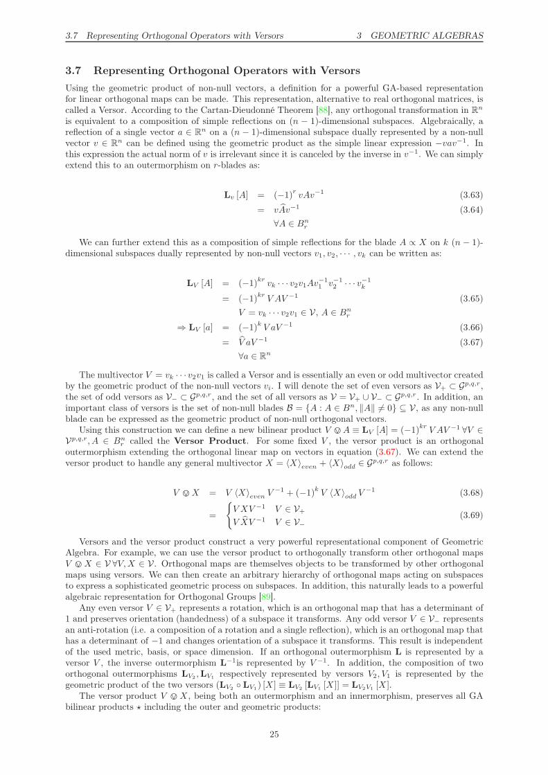
3.7 Representing Orthogonal Operators with Versors 3 GEOMETRIC ALGEBRAS

3.7 Representing Orthogonal Operators with Versors

Using the geometric product of non-null vectors, a definition for a powerful GA-based representationfor linear orthogonal maps can be made. This representation, alternative to real orthogonal matrices, iscalled a Versor. According to the Cartan-Dieudonné Theorem [88], any orthogonal transformation in Rn

is equivalent to a composition of simple reflections on (n − 1)-dimensional subspaces. Algebraically, areflection of a single vector a ∈ Rn on a (n − 1)-dimensional subspace dually represented by a non-nullvector v ∈ Rn can be defined using the geometric product as the simple linear expression −vav−1. Inthis expression the actual norm of v is irrelevant since it is canceled by the inverse in v−1. We can simplyextend this to an outermorphism on r-blades as:

Lv [A] = (−1)r vAv−1 (3.63)

= vAv−1 (3.64)

∀A ∈ Bnr

We can further extend this as a composition of simple reflections for the blade A ∝ X on k (n − 1)-dimensional subspaces dually represented by non-null vectors v1, v2, · · · , vk can be written as:

LV [A] = (−1)kr vk · · · v2v1Av−11 v−1

2 · · · v−1k

= (−1)kr V AV −1 (3.65)

V = vk · · · v2v1 ∈ V , A ∈ Bnr

⇒ LV [a] = (−1)k V aV −1 (3.66)

= V aV −1 (3.67)

∀a ∈ Rn

The multivector V = vk · · · v2v1 is called a Versor and is essentially an even or odd multivector createdby the geometric product of the non-null vectors vi. I will denote the set of even versors as V+ ⊂ Gp,q,r,the set of odd versors as V− ⊂ Gp,q,r, and the set of all versors as V = V+ ∪ V− ⊂ Gp,q,r . In addition, animportant class of versors is the set of non-null blades B = {A : A ∈ Bn, ‖A‖ 6= 0} ⊆ V , as any non-nullblade can be expressed as the geometric product of non-null orthogonal vectors.

Using this construction we can define a new bilinear product V 6A ≡ LV [A] = (−1)kr V AV −1 ∀V ∈Vp,q,r, A ∈ Bn

r called the Versor Product. For some fixed V , the versor product is an orthogonaloutermorphism extending the orthogonal linear map on vectors in equation (3.67). We can extend theversor product to handle any general multivector X = 〈X〉even + 〈X〉odd ∈ G

p,q,r as follows:

V 6 X = V 〈X〉even V −1 + (−1)k V 〈X〉odd V−1 (3.68)

=

{V XV −1 V ∈ V+

V XV −1 V ∈ V−(3.69)

Versors and the versor product construct a very powerful representational component of GeometricAlgebra. For example, we can use the versor product to orthogonally transform other orthogonal mapsV 6 X ∈ V ∀V,X ∈ V . Orthogonal maps are themselves objects to be transformed by other orthogonalmaps using versors. We can then create an arbitrary hierarchy of orthogonal maps acting on subspacesto express a sophisticated geometric process on subspaces. In addition, this naturally leads to a powerfulalgebraic representation for Orthogonal Groups [89].

Any even versor V ∈ V+ represents a rotation, which is an orthogonal map that has a determinant of1 and preserves orientation (handedness) of a subspace it transforms. Any odd versor V ∈ V− representsan anti-rotation (i.e. a composition of a rotation and a single reflection), which is an orthogonal map thathas a determinant of −1 and changes orientation of a subspace it transforms. This result is independentof the used metric, basis, or space dimension. If an orthogonal outermorphism L is represented by aversor V , the inverse outermorphism L−1is represented by V −1. In addition, the composition of twoorthogonal outermorphisms LV2

,LV1respectively represented by versors V2, V1 is represented by the

geometric product of the two versors (LV2◦ LV1

) [X ] ≡ LV2[LV1

[X ]] = LV2V1[X ].

The versor product V 6 X , being both an outermorphism and an innermorphism, preserves all GAbilinear products ⋆ including the outer and geometric products:

25

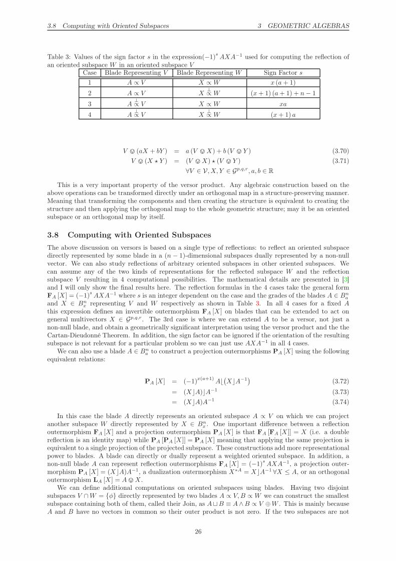
3.8 Computing with Oriented Subspaces 3 GEOMETRIC ALGEBRAS

Table 3: Values of the sign factor s in the expression(−1)s AXA−1 used for computing the reflection ofan oriented subspace W in an oriented subspace V

Case Blade Representing V Blade Representing W Sign Factor s

1 A ∝ V X ∝W x (a+ 1)

2 A ∝ V X⊥∝W (x+ 1) (a+ 1) + n− 1

3 A⊥∝ V X ∝W xa

4 A⊥∝ V X

⊥∝W (x+ 1) a

V 6 (aX + bY ) = a (V 6 X) + b (V 6 Y ) (3.70)

V 6 (X ⋆ Y ) = (V 6 X) ⋆ (V 6 Y ) (3.71)

∀V ∈ V , X, Y ∈ Gp,q,r, a, b ∈ R

This is a very important property of the versor product. Any algebraic construction based on theabove operations can be transformed directly under an orthogonal map in a structure-preserving manner.Meaning that transforming the components and then creating the structure is equivalent to creating thestructure and then applying the orthogonal map to the whole geometric structure; may it be an orientedsubspace or an orthogonal map by itself.

3.8 Computing with Oriented Subspaces

The above discussion on versors is based on a single type of reflections: to reflect an oriented subspacedirectly represented by some blade in a (n − 1)-dimensional subspaces dually represented by a non-nullvector. We can also study reflections of arbitrary oriented subspaces in other oriented subspaces. Wecan assume any of the two kinds of representations for the reflected subspace W and the reflectionsubspace V resulting in 4 computational possibilities. The mathematical details are presented in [3]and I will only show the final results here. The reflection formulas in the 4 cases take the general formFA [X ] = (−1)s AXA−1 where s is an integer dependent on the case and the grades of the blades A ∈ Bn

a

and X ∈ Bnx representing V and W respectively as shown in Table 3. In all 4 cases for a fixed A

this expression defines an invertible outermorphism FA [X ] on blades that can be extended to act ongeneral multivectors X ∈ Gp,q,r. The 3rd case is where we can extend A to be a versor, not just anon-null blade, and obtain a geometrically significant interpretation using the versor product and the theCartan-Dieudonné Theorem. In addition, the sign factor can be ignored if the orientation of the resultingsubspace is not relevant for a particular problem so we can just use AXA−1 in all 4 cases.

We can also use a blade A ∈ Bna to construct a projection outermorphisms PA [X ] using the following

equivalent relations:

PA [X ] = (−1)x(a+1)A⌊(X⌋A−1

)(3.72)

= (X⌋A)⌋A−1 (3.73)

= (X⌋A)A−1 (3.74)

In this case the blade A directly represents an oriented subspace A ∝ V on which we can projectanother subspace W directly represented by X ∈ Bn

x . One important difference between a reflectionoutermorphism FA [X ] and a projection outermorphism PA [X ] is that FA [FA [X ]] = X (i.e. a doublereflection is an identity map) while PA [PA [X ]] = PA [X ] meaning that applying the same projection isequivalent to a single projection of the projected subspace. These constructions add more representationalpower to blades. A blade can directly or dually represent a weighted oriented subspace. In addition, anon-null blade A can represent reflection outermorphisms FA [X ] = (−1)s AXA−1, a projection outer-morphism PA [X ] = (X⌋A)A−1, a dualization outermorphism X∗A = X⌋A−1 ∀X ≤ A, or an orthogonaloutermorphism LA [X ] = A 6 X .

We can define additional computations on oriented subspaces using blades. Having two disjointsubspaces V ∩W = {φ} directly represented by two blades A ∝ V,B ∝W we can construct the smallestsubspace containing both of them, called their Join, as A⊔B ≡ A∧B ∝ V ⊕W . This is mainly becauseA and B have no vectors in common so their outer product is not zero. If the two subspaces are not

26

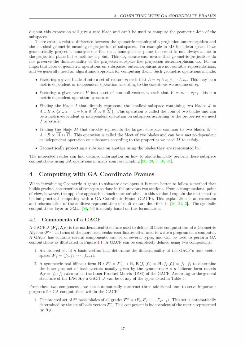
4 COMPUTING WITH GA COORDINATE FRAMES

disjoint this expression will give a zero blade and can’t be used to compute the geometric Join of thesubspaces.

There exists a related difference between the geometric meaning of a projection outermorphism andthe classical geometric meaning of projection of subspaces. For example in 3D Euclidean space, if wegeometrically project a homogeneous line on a homogeneous plane the result is not always a line inthe projection plane but sometimes a point. This degenerate case means that geometric projections donot preserve the dimensionality of the projected subspace like projection outermorphisms do. For animportant class of geometric operations on subspaces, outermorphisms are not suitable representations,and we generally need an algorithmic approach for computing them. Such geometric operations include:

• Factoring a given blade A into a set of vectors vi such that A = v1 ∧ v1 ∧ · · · ∧ vr. This may be ametric-dependent or independent operation according to the conditions we assume on vi.

• Factoring a given versor V into a set of non-null vectors vi such that V = vr · · · v2v1. his is ametric-dependent operation by nature.

• Finding the blade J that directly represents the smallest subspace containing two blades J =

A ⊔ B ∝ {x :: x = a + b; a ∈←→A , b ∈

←→B }. This operation is called the Join of two blades and can

be a metric-dependent or independent operation on subspaces according to the properties we needJ to satisfy.

• Finding the blade M that directly represents the largest subspace common to two blades M =

A ⊓ B ∝←→A ∩

←→B . This operation is called the Meet of two blades and can be a metric-dependent

or independent operation on subspaces according to the properties we need M to satisfy.

• Geometrically projecting a subspace on another using the blades they are represented by.

The interested reader can find detailed information on how to algorithmically perform these subspacecomputations using GA operations in many sources including [90, 20, 3, 10, 91].

4 Computing with GA Coordinate Frames

When introducing Geometric Algebra to software developers it is much better to follow a method thatbuilds gradual construction of concepts as done in the previous two sections. From a computational pointof view, however, the opposite approach is much more suitable. In this section I explain the mathematicsbehind practical computing with a GA Coordinate Frame (GACF). This explanation is an extensionand reformulation of the additive representation of multivectors described in [20, 21, 3]. The symboliccomputations layer in GMac [58, 59] is mainly based on this formulation.

4.1 Components of a GACF

A GACF F (F n1 ,AF ) is the mathematical structure used to define all basic computations of a Geometric

Algebra Gp,q,r in terms of the more basic scalar coordinates often used to write a program on a computer.A GACF has contains several components, can be of several types, and can be used to perform GAcomputations as illustrated in Figure 4.1. A GACF can be completely defined using two components:

1. An ordered set of n basis vectors that determine the dimensionality of the GACF’s base vectorspace: F

n1 = 〈f0, f1, · · · , fn−1〉.

2. A symmetric real bilinear form B : F n1 × F

n1 → R, B (fi, fj) = B (fj , fi) = fi · fj to determine

the inner product of basis vectors usually given by the symmetric n × n bilinear form matrixAF = [fi · fj]; also called the Inner Product Matrix (IPM) of the GACF. According to the generalstructure of the IPM AF a GACF F can be of any of the types listed in Table 4.

From these two components, we can automatically construct three additional ones to serve importantpurposes for GA computations within the GACF:

1. The ordered set of 2n basis blades of all grades F n = 〈F0, F1, · · · , F2n−1〉. This set is automaticallydetermined by the set of basis vectors F n

1 . This component is independent of the metric representedby AF .

27

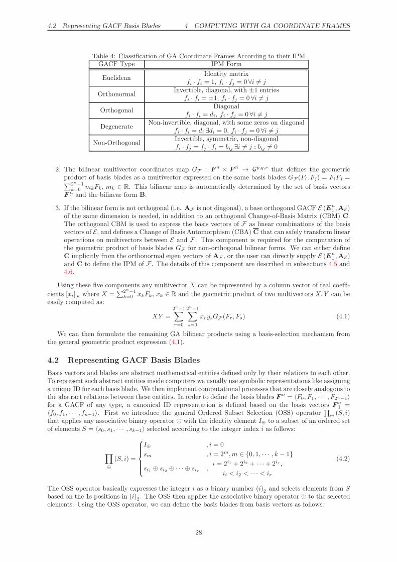
4.2 Representing GACF Basis Blades 4 COMPUTING WITH GA COORDINATE FRAMES

Table 4: Classification of GA Coordinate Frames According to their IPMGACF Type IPM Form

EuclideanIdentity matrix

fi · fi = 1, fi · fj = 0 ∀i 6= j

OrthonormalInvertible, diagonal, with ±1 entries

fi · fi = ±1, fi · fj = 0 ∀i 6= j

OrthogonalDiagonal

fi · fi = di, fi · fj = 0 ∀i 6= j

DegenerateNon-invertible, diagonal, with some zeros on diagonal

fi · fi = di ∃di = 0, fi · fj = 0 ∀i 6= j

Non-OrthogonalInvertible, symmetric, non-diagonalfi · fj = fj · fi = bij ∃i 6= j : bij 6= 0

2. The bilinear multivector coordinates map GF : Fn × F

n → Gp,q,r that defines the geometricproduct of basis blades as a multivector expressed on the same basis blades GF (Fi, Fj) = FiFj =∑2n−1

k=0 mkFk, mk ∈ R. This bilinear map is automatically determined by the set of basis vectorsF

n1 and the bilinear form B.

3. If the bilinear form is not orthogonal (i.e. AF is not diagonal), a base orthogonal GACF E (En1 ,AE)

of the same dimension is needed, in addition to an orthogonal Change-of-Basis Matrix (CBM) C.The orthogonal CBM is used to express the basis vectors of F as linear combinations of the basisvectors of E , and defines a Change of Basis Automorphism (CBA) C that can safely transform linearoperations on multivectors between E and F . This component is required for the computation ofthe geometric product of basis blades GF for non-orthogonal bilinear forms. We can either defineC implicitly from the orthonormal eigen vectors of AF , or the user can directly supply E (En

1 ,AE)and C to define the IPM of F . The details of this component are described in subsections 4.5 and4.6.

Using these five components any multivector X can be represented by a column vector of real coeffi-cients [xi]F where X =

∑2n−1k=0 xkFk, xk ∈ R and the geometric product of two multivectors X,Y can be

easily computed as:

XY =

2n−1∑

r=0

2n−1∑

s=0

xrysGF (Fr, Fs) (4.1)

We can then formulate the remaining GA bilinear products using a basis-selection mechanism fromthe general geometric product expression (4.1).

4.2 Representing GACF Basis Blades

Basis vectors and blades are abstract mathematical entities defined only by their relations to each other.To represent such abstract entities inside computers we usually use symbolic representations like assigninga unique ID for each basis blade. We then implement computational processes that are closely analogous tothe abstract relations between these entities. In order to define the basis blades F n = 〈F0, F1, · · · , F2n−1〉for a GACF of any type, a canonical ID representation is defined based on the basis vectors F

n1 =

〈f0, f1, · · · , fn−1〉. First we introduce the general Ordered Subset Selection (OSS) operator∏

⊕(S, i)

that applies any associative binary operator ⊕ with the identity element I⊕ to a subset of an ordered setof elements S = 〈s0, s1, · · · , sk−1〉 selected according to the integer index i as follows:

∏

⊕

(S, i) =

I⊕ , i = 0

sm , i = 2m,m ∈ {0, 1, · · · , k − 1}

si1 ⊕ si2 ⊕ · · · ⊕ sir ,i = 2i1 + 2i2 + · · ·+ 2ir ,

ii < i2 < · · · < ir

(4.2)

The OSS operator basically expresses the integer i as a binary number (i)2 and selects elements from S

based on the 1s positions in (i)2. The OSS then applies the associative binary operator ⊕ to the selectedelements. Using the OSS operator, we can define the basis blades from basis vectors as follows:

28

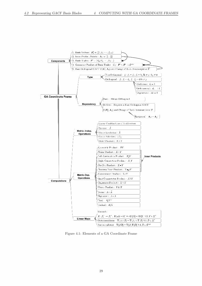
4.2 Representing GACF Basis Blades 4 COMPUTING WITH GA COORDINATE FRAMES

Figure 4.1: Elements of a GA Coordinate Frame

29

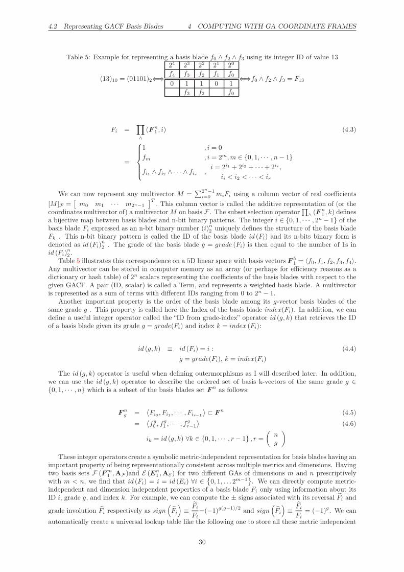
4.2 Representing GACF Basis Blades 4 COMPUTING WITH GA COORDINATE FRAMES

Table 5: Example for representing a basis blade f0 ∧ f2 ∧ f3 using its integer ID of value 13

(13)10 = (01101)2⇐⇒

24 23 22 21 20

f4 f3 f2 f1 f0

0 1 1 0 1f3 f2 f0

⇐⇒f0 ∧ f2 ∧ f3 = F13

Fi =∏

∧

(F n1 , i) (4.3)

=

1 , i = 0

fm , i = 2m,m ∈ {0, 1, · · · , n− 1}

fi1 ∧ fi2 ∧ · · · ∧ fir ,i = 2i1 + 2i2 + · · ·+ 2ir ,

ii < i2 < · · · < ir

We can now represent any multivector M =∑2n−1

i=0 miFi using a column vector of real coefficients

[M ]F =[m0 m1 · · · m2n−1

]T. This column vector is called the additive representation of (or the

coordinates multivector of) a multivector M on basis F . The subset selection operator∏

∧(F n

1 , k) definesa bijective map between basis blades and n-bit binary patterns. The integer i ∈ {0, 1, · · · , 2n − 1} of thebasis blade Fi expressed as an n-bit binary number (i)n2 uniquely defines the structure of the basis bladeFk . This n-bit binary pattern is called the ID of the basis blade id (Fi) and its n-bits binary form isdenoted as id (Fi)

n2 . The grade of the basis blade g = grade (Fi) is then equal to the number of 1s in

id (Fi)n2 .

Table 5 illustrates this correspondence on a 5D linear space with basis vectors F 51 = 〈f0, f1, f2, f3, f4〉.

Any multivector can be stored in computer memory as an array (or perhaps for efficiency reasons as adictionary or hash table) of 2n scalars representing the coefficients of the basis blades with respect to thegiven GACF. A pair (ID, scalar) is called a Term, and represents a weighted basis blade. A multivectoris represented as a sum of terms with different IDs ranging from 0 to 2n − 1.

Another important property is the order of the basis blade among its g-vector basis blades of thesame grade g . This property is called here the Index of the basis blade index(Fi). In addition, we candefine a useful integer operator called the “ID from grade-index” operator id (g, k) that retrieves the IDof a basis blade given its grade g = grade(Fi) and index k = index (Fi):

id (g, k) ≡ id (Fi) = i : (4.4)

g = grade(Fi), k = index(Fi)

The id (g, k) operator is useful when defining outermorphisms as I will described later. In addition,we can use the id (g, k) operator to describe the ordered set of basis k-vectors of the same grade g ∈{0, 1, · · · , n} which is a subset of the basis blades set F

n as follows:

Fng =

⟨Fi0 , Fi1 , · · · , Fir−1

⟩⊂ F

n (4.5)

=⟨fg0 , f

g1 , · · · , f

gr−1

⟩(4.6)

ik = id (g, k) ∀k ∈ {0, 1, · · · , r − 1} , r =

(n

g

)

These integer operators create a symbolic metric-independent representation for basis blades having animportant property of being representationally consistent across multiple metrics and dimensions. Havingtwo basis sets F (Fm

1 ,AF )and E (En1 ,AE) for two different GAs of dimensions m and n prescriptively

with m < n, we find that id (Fi) = i = id (Ei) ∀i ∈{0, 1, . . .2m−1

}. We can directly compute metric-

independent and dimension-independent properties of a basis blade Fi only using information about itsID i, grade g, and index k. For example, we can compute the ± signs associated with its reversal Fi and

grade involution Fi respectively as sign(Fi

)≡

Fi

Fi=(−1)g(g−1)/2 and sign

(Fi

)≡

Fi

Fi= (−1)g. We can

automatically create a universal lookup table like the following one to store all these metric independent

30

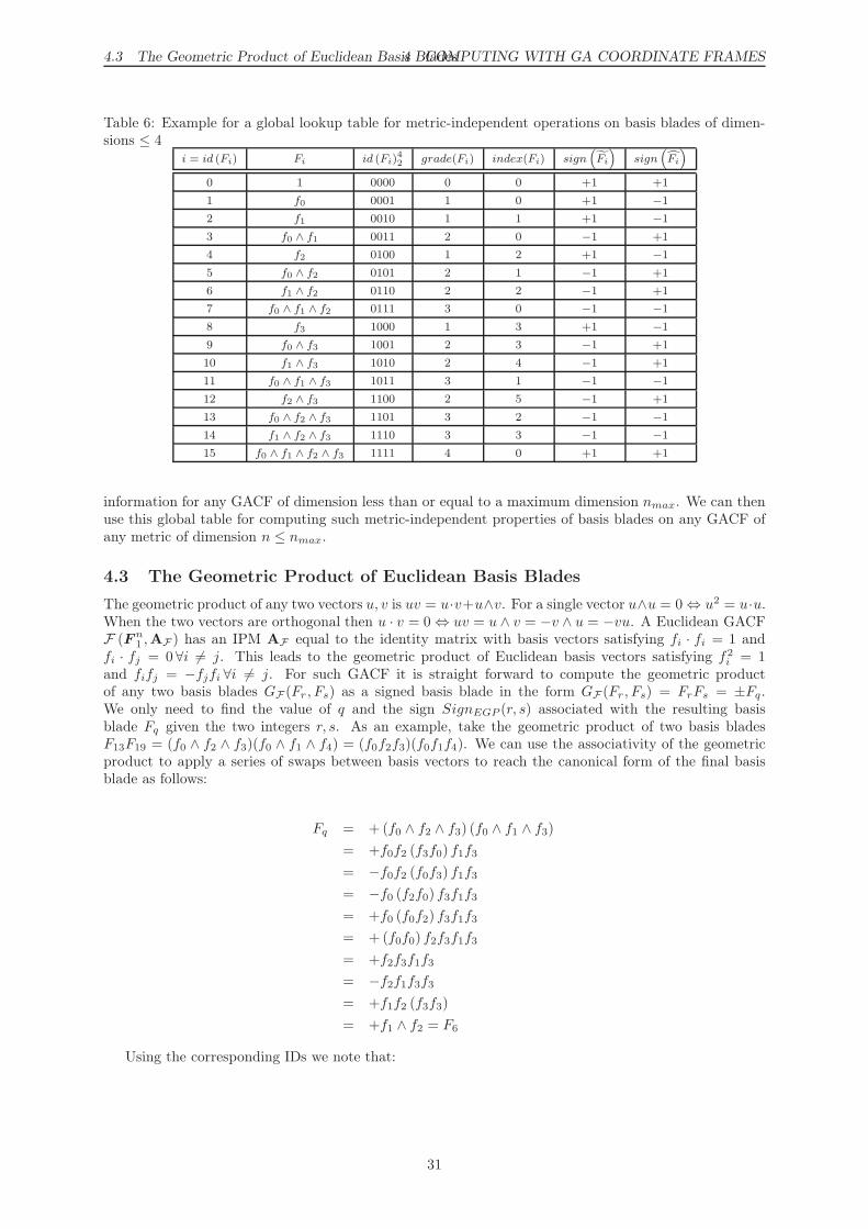
4.3 The Geometric Product of Euclidean Basis Blades4 COMPUTING WITH GA COORDINATE FRAMES

Table 6: Example for a global lookup table for metric-independent operations on basis blades of dimen-sions ≤ 4

i = id (Fi) Fi id (Fi)4

2grade(Fi) index(Fi) sign

(Fi

)sign

(Fi

)

0 1 0000 0 0 +1 +1

1 f0 0001 1 0 +1 −1

2 f1 0010 1 1 +1 −1

3 f0 ∧ f1 0011 2 0 −1 +1

4 f2 0100 1 2 +1 −1

5 f0 ∧ f2 0101 2 1 −1 +1

6 f1 ∧ f2 0110 2 2 −1 +1

7 f0 ∧ f1 ∧ f2 0111 3 0 −1 −1

8 f3 1000 1 3 +1 −1

9 f0 ∧ f3 1001 2 3 −1 +1

10 f1 ∧ f3 1010 2 4 −1 +1

11 f0 ∧ f1 ∧ f3 1011 3 1 −1 −1

12 f2 ∧ f3 1100 2 5 −1 +1

13 f0 ∧ f2 ∧ f3 1101 3 2 −1 −1

14 f1 ∧ f2 ∧ f3 1110 3 3 −1 −1

15 f0 ∧ f1 ∧ f2 ∧ f3 1111 4 0 +1 +1

information for any GACF of dimension less than or equal to a maximum dimension nmax. We can thenuse this global table for computing such metric-independent properties of basis blades on any GACF ofany metric of dimension n ≤ nmax.

4.3 The Geometric Product of Euclidean Basis Blades

The geometric product of any two vectors u, v is uv = u·v+u∧v. For a single vector u∧u = 0⇔ u2 = u·u.When the two vectors are orthogonal then u · v = 0⇔ uv = u ∧ v = −v ∧ u = −vu. A Euclidean GACFF (F n

1 ,AF ) has an IPM AF equal to the identity matrix with basis vectors satisfying fi · fi = 1 andfi · fj = 0 ∀i 6= j. This leads to the geometric product of Euclidean basis vectors satisfying f2

i = 1and fifj = −fjfi ∀i 6= j. For such GACF it is straight forward to compute the geometric productof any two basis blades GF (Fr , Fs) as a signed basis blade in the form GF (Fr , Fs) = FrFs = ±Fq.We only need to find the value of q and the sign SignEGP (r, s) associated with the resulting basisblade Fq given the two integers r, s. As an example, take the geometric product of two basis bladesF13F19 = (f0 ∧ f2 ∧ f3)(f0 ∧ f1 ∧ f4) = (f0f2f3)(f0f1f4). We can use the associativity of the geometricproduct to apply a series of swaps between basis vectors to reach the canonical form of the final basisblade as follows:

Fq = +(f0 ∧ f2 ∧ f3) (f0 ∧ f1 ∧ f3)

= +f0f2 (f3f0) f1f3

= −f0f2 (f0f3) f1f3

= −f0 (f2f0) f3f1f3

= +f0 (f0f2) f3f1f3

= +(f0f0) f2f3f1f3

= +f2f3f1f3

= −f2f1f3f3

= +f1f2 (f3f3)

= +f1 ∧ f2 = F6

Using the corresponding IDs we note that:

31

4.4 The Geometric Product of Orthogonal Basis Blades4 COMPUTING WITH GA COORDINATE FRAMES

Algorithm 1 SignEGP (r, s): Computes the sign of the geometric product FrFs of two Euclidean basisblades Fr, Fs ∈ Gn,0,0

1. Initialize the sign variable S ← +1 and the ID variables idr ← id (Fr), ids ← id (Fs)

2. For increasing i from 0 to n− 1 do steps 3-6:

3. If bit i in (ids)n2 is a 1 do:

4. For decreasing j from n− 1 to i+ 1 do step 5:

5. If bit j in (idr)n2 is a 1 Then set S ← −S

6. If bit i in (idr)n2 is a 1 Then set it to 0 Else set it to 1

7. Return final result in S

id (f1 ∧ f2)42 = 0110

= 1011 XOR 1101

= id (f0 ∧ f1 ∧ f3)42 XOR id (f0 ∧ f2 ∧ f3)

42

This is not a coincidence because if the same basis vector fi is present or absent in both input basisblades it will always be absent in the final basis blade due to the property f2

i = 1, and if a basis vectoris only present in one of the input basis blades it’s always present in the final basis blade. Hence we canfind the ID of the final basis blade Fq by a bit-wise XOR operation between the IDs of the input basisblades Fr, Fs:

FrFs = SignEGP (r, s)Fq (4.7)

(q)2 = id (Fq)n2 = id (Fr)

n2 XOR id (Fs)

n2

= (r)n2 XOR (s)

n2 (4.8)

∀r, s ∈ {0, 1, . . . , 2n − 1}

We can compute the sign of the final geometric product term using Algorithm 1 or a similar variant.Using such algorithm, we can construct a Euclidean Geometric Product Sign lookup table having 2n−1

rows and 2n − 1 columns where each cell at row i and column j contains the number SignEGP (Fi, Fj). Although this table is specific to Euclidean metric of dimension n, we can use it to compute theEuclidean geometric product of basis blades of any dimension m ≤ n because of the universal property ifthis method of representation. In addition, we can compute the geometric product of basis blades havingother metrics based on the signs in this Euclidean table, as I will show shortly. An important propertyfor SignEGP (i, i) is:

F 2i = FiFi

= Fi

(Fi

)∼

= (−1)g(g−1)/2FiFi

= (−1)g(g−1)/2

⇒ SignEGP (i, i) = (−1)g(g−1)/2, g = grade (Fi) (4.9)

∀i ∈ {0, 1, . . . , 2n − 1}

4.4 The Geometric Product of Orthogonal Basis Blades

An orthogonal GACF F (F n1 ,AF ) has a diagonal IPM AF with basis vectors satisfying fi · fi = di

and fi · fj = 0 ∀i 6= j leading to the geometric product of orthogonal basis vectors satisfying f2i = di

and fifj = −fjfi ∀i 6= j. The only difference between a Euclidean GACF and an orthogonal GACFis that the square of a basis vector can be any real number di, including negative numbers and zero.

32

4.5 Constructing a Derived GACF 4 COMPUTING WITH GA COORDINATE FRAMES

The same algorithm applied for a Euclidean GACF can thus be used to deduce a geometric product forsuch GACF with a single change to step 5 to become: “If bit i in (idr)

n2 is a 1 Then set it to 0 and set

S ← diS Else set it to 1”. We could then create a similar lookup table for each orthogonal GACF inour problem. There is a better alternative in this case, however, by using the geometric product for aEuclidean GACF E (En

1 ,AE) with the same dimension having basis blades En = 〈E0, E1, · · · , E2n−1〉.

If ErEs = SignEGP (r, s)Ek then FrFs = SignEGP (r, s)λkFk where λk =∏

(〈d0, d1, · · · , dn−1〉 , k) =

FkFk = ‖Fk‖, called the signature of Fk, is the multiplication of all di having a corresponding 1-bit inthe bit pattern (k)

n2 = id (Fk)

n2 = id (Ek)

n2 = (r)

n2 XOR (s)

n2 . This leads to a save in memory by only

storing 2n scalar values λk = FkFk, k ∈ {0, 1, · · · , 2n − 1} for each orthogonal GACF, then the EuclideanGeometric Product Sign lookup table is used to compute FrFs as follows:

FrFs = SignEGP (r, s)λkFk (4.10)

(k)n2 = (r)n2 XOR (s)n2 (4.11)

∀r, s ∈ {0, 1, . . . , 2n − 1}

When the orthogonal GACF is degenerate we have some null basis vectors with di = 0 and subse-quently we find the basis blade signatures λk computed from these null basis vectors will also equal zero.For degenerate orthogonal GACFs we have to be careful when computing with null basis blades in someGA operations; for example when we need to divide by the norm of a blade we must take care not to usenull blades.

4.5 Constructing a Derived GACF

Having a general GACF E (En1 ,AE) with basis vectors E

n1 = 〈e0, e1, · · · , en−1〉 we can use an invertible

Change-of-Basis Matrix C = [cij ] to define a new derived set of basis vectors F n1 = 〈f0, f1, · · · , fn−1〉 for

the same linear space as fi =∑n−1

j=0 cijej ∀i ∈ {0, 1, · · · , n− 1}. If a vector x is represented on the basis

En1 by the column vector [x]En

1

=[x0 x1 · · · xn−1

]Tand on the basis F

n1 by the column vector

[x]Fn1

=[y0 y1 · · · yn−1

]Twe find that:

[x]En1

= CT [x]Fn1

(4.12)

⇔ [x]Fn1

= C−T [x]En1

(4.13)

In the special case that C is orthogonal C−1 = CT we get [x]Fn1

= C [x]En1

. The elements of thederived IPM AF = [fi · fj ] can be easily calculated from the IPM AE = [ei · ej ] as follows for anyinvertible C:

fi · fj =

(n−1∑

r=0

cirer

)·

(n−1∑

s=0

cjses

)

=

n−1∑

s=0

n−1∑

r=0

circjs(er · es)

=

n−1∑

s=0

(n−1∑

r=0

cir(er · es)

)cTsj

⇒ AF = CAECT (4.14)

Using Fn1 and AF we can then construct a derived GACF F (F n

1 ,AF) relative to the given base GACFE (En

1 ,AE) by means of the invertible CBM C. To compute the geometric product of multivectors onthe derived GACF we have 3 separate cases:

• In the case when AF is diagonal then F is an orthogonal GACF and the geometric product of twomultivectors represented on F can be computed using the method in the previous subsection.

• When AF is not diagonal but the base GACF E is orthogonal and C is an orthogonal CBMC−1 = CT , the geometric product of the derived basis blades F n can be computed by extending P =

CT = C−1 and PT = C−T = C as two adjoint orthogonal outermorphisms P and PTrespectively.

33

4.6 Constructing a Non-Orthogonal GACF 4 COMPUTING WITH GA COORDINATE FRAMES

These two outermorphisms preserve all bilinear products including the geometric product. We cansafely use P and P

Tto transform bilinear products of multivectors back and forth between the

base GACF E and the derived GACF F . Any bilinear product ⋆ of two multivectors X,Y can becomputed on the derived GACF F as:

XY = P[P

T[X ] ⋆P

T[Y ]], P = C

T,P

T= P

−1(4.15)

• When AF is not diagonal and either E is not orthogonal or C is not an orthogonal CBM, an-other method for computing the geometric product is needed, which is explained in the followingsubsection.

4.6 Constructing a Non-Orthogonal GACF

We can directly define a non-orthogonal GACF F (F n1 ,AF ) using a given non-diagonal symmetric real

IPM AF . For a non-orthogonal GACF F the geometric product of any two basis blades is not guaranteedto be a term (i.e. a weighted basis blade) but is generally a multivector (i.e. the sum of terms of differentbasis blades). If we try to make a geometric product lookup table for such GACF, each cell in thelookup table would then be a full multivector that may contain up to 2n terms. This is a lot to store inmemory for a single GACF; 23n terms many of which are typically zeros. A better alternative is to usea diagonalization technique on the IPM AF to express the non-orthogonal GACF as a derived GACFfrom a base orthogonal GACF E (En

1 ,AE) with basis vectors En1 = 〈e0, e1, · · · , en−1〉. This is done by

finding the IPM AE of the base orthogonal GACF and the orthogonal CBM C = [cij ] ,C−1 = CT that

expresses the basis vectors in Fn1 as linear combinations of the orthogonal basis vectors in E

n1 using

fi =∑n−1

j=0 cijej ∀i ∈ {0, 1, · · · , n− 1} as explained in the previous subsection. This time we already haveAF and we need to compute AE and C.

Noting that the IPM AF is a symmetric real matrix, it is easy to find the real eigen values di and n

corresponding orthonormal eigen column vectors Vi of AF that satisfy AFVi = diVi, VTi Vj = 0 ∀i, j ∈

{0, 1, · · · , n− 1}. We can then create an orthogonal matrix P =[V1 V2 · · · Vn

],P−1 = PT as a

concatenation of the orthonormal column vectors Vi. The matrix AE = PTAFP is actually a diagonalmatrix containing the eigen values di on its diagonal. Hence AE can be considered the IPM of a baseorthogonal GACF from which we derive the non-orthogonal GACF F (F n

1 ,AF ). Now we can use equation(4.15) to compute any bilinear product on two multivectors as before. This means that for each non-

orthogonal GACF F it is necessary to construct and store the orthogonal outermorphisms PT

and P

created through an eigen analysis of AF .

4.7 Constructing a Reciprocal GACF

Having a general non-degenerate GACF E (En1 ,AE)with basis vectors E

n1 = 〈e0, e1, · · · , en−1〉 and non-

null basis blades, it is possible to create a special type of derived GACF called the Reciprocal GACFF (F n

1 ,AF ) having non-null basis vectors Fn1 = 〈f0, f1, · · · , fn−1〉 using the relations [3]:

fi = (−1)i−1 (e1 ∧ e2 ∧ · · · ∧ ei−1 ∧ ei+1 ∧ · · · ∧ en)⌋I−1 (4.16)

I = e1 ∧ e2 ∧ · · · ∧ en,

I−1 =(−1)n(n−1)/2

III

⇒ fi · ej = δij , (4.17)

fi · fj = ei · ej (4.18)

∀i, j ∈ {0, 1, · · · , n− 1}

⇔ AF = A−1E

(4.19)

If the base GACF E is orthogonal the derived reciprocal GACF F is also orthogonal and the aboverelations reduce to the simpler form:

fi =1

ei · eiei ∀i ∈ {0, 1, · · · , n− 1} (4.20)

⇔ AF = A−1E

= A−1E

(4.21)

34

4.8 Computing Bilinear Products on a GACF4 COMPUTING WITH GA COORDINATE FRAMES

For a non-orthogonal base GACF E the reciprocal GACF F is also non-orthogonal. We can then useequation (4.19) to compute AF and then find the orthogonal CBM P and continue as described in theprevious subsection.

4.8 Computing Bilinear Products on a GACF

Starting with orthogonal GACFs, any bilinear product ⋆ of two multivectors X,Y ∈ Gp,q,r performed ontheir representations [X ]

F, [Y ]

Fin an orthogonal GACF F (F n

1 ,AF) with basis blades F n = 〈F0, F1, · · · , F2n−1〉can be implemented as:

X ⋆ Y =2n−1∑

r=0

2n−1∑

s=0

xrys (Fr ⋆ Fs) (4.22)

The goal is to find the value of Fr ⋆ Fs for all r, s ∈ {0, 1, · · · , 2n − 1}. Due to the properties of thegeometric product on orthogonal frames and the definitions of the bilinear products, the bilinear productof any two basis blades Fr ⋆ Fs is either a zero or a single term λ⋆

kFk, but never more than a single term.Actually when the value of Fr ⋆ Fs = λ⋆

kFk the term is equal to the geometric product of the two basisblades λ⋆

kFk = GF (Fr, Fs) = FrFs. Assuming a = grade (Fr) and b = grade (Fs), the following relationslist some useful GA bilinear products and their relations with the geometric product on the basis blades:

Scalar Product:

Fr ∗ Fs = 〈FrFs〉0 (4.23)

=

{0 (r)2 XOR (s)2 6= (0)2FrFs otherwise

(4.24)

Left Contraction Product:

Fr⌋Fs = 〈FrFs〉b−a (4.25)

=

{0 (r)2 AND NOT (s)2 6= (0)2FrFs otherwise

(4.26)

Right Contraction Product:

Fr⌊Fs = 〈FrFs〉a−b (4.27)

=

{0 (s)2 AND NOT (r)2 6= (0)2FrFs otherwise

(4.28)

Fat-Dot Product:

Fr • Fs = 〈FrFs〉0 + 〈FrFs〉b−a + 〈FrFs〉a−b (4.29)

=

0 a = b, (r)2 XOR (s)2 6= (0)20 a < b, (r)2 AND NOT (s)2 6= (0)20 a > b, (s)2 AND NOT (r)2 6= (0)2FrFs otherwise

(4.30)

Hestenes Inner Product:

Fr •H Fs =

{Fr • Fs ab > 0

0 ab = 0(4.31)

=

0 ab > 0, a = b, (r)2 XOR (s)2 6= (0)20 ab > 0, a < b, (r)2 AND NOT (s)2 6= (0)20 ab > 0, a > b, (s)2 AND NOT (r)2 6= (0)20 ab = 0

FrFs otherwise

(4.32)

35

4.9 Computing Linear Maps on GACFs 4 COMPUTING WITH GA COORDINATE FRAMES

Commutator Product:

Fr×Fs =1

2(FrFs − FsFr) (4.33)

=

{0 SignEGP (r, s) = SignEGP (s, r)

FrFs otherwise(4.34)

Anti-Commutator Product:

Fr×Fs =1

2(FrFs + FsFr) (4.35)

=

{0 SignEGP (r, s) 6= SignEGP (s, r)

FrFs otherwise(4.36)

One exception to this pattern is the Outer Product that is metric-independent, and can’t be com-puted from the metric-dependent geometric product. Based on the discussion in section 4.3 we can assumea Euclidean GACF with the same dimension N (Nn

1 , In) with no loss of generality and then compute theouter product Fr ∧ Fs from the geometric product on the Euclidean GACF N :

Fr ∧ Fs = Nr ∧Ns (4.37)

= 〈NrNs〉a+b (4.38)

=

{0 (r)2 AND (s)2 6= (0)2NrNs otherwise

(4.39)

Another exception is the Regressive Product that we can compute given two multivectors X,Y

using other bilinear products. This particular product has several definitions in the literature. Thefollowing is just one of them:

X ∨ Y = (X∗ ∧ Y ∗)⊙ (4.40)

=(XI−1 ∧ Y I−1

)I (4.41)

For a non-orthogonal GACF F a bilinear product of two basis blades is not guaranteed to producea single term, except for the outer product. All the above computational relations become invalid inthis case. We can use equation (4.15) to compute any metric-dependent bilinear product from the two

orthogonal outermorphisms PT

and P associated with F .

4.9 Computing Linear Maps on GACFs

Any Grassmann Space∧n is a linear space with 2n basis blades. We can define and use general linear

maps between two Grassmann spaces T :∧n →

∧m and use any given bases E (En1 ,AE) and F (Fm

1 ,AF )on the two spaces to create a (2m − 1)×(2n − 1) representation matrix MT =

[M0 M1 · · · M2n−1

]

for T on the two bases where the column vectors Mk = [T [Ek]]F represent the transformed basis bladesin E using the basis blades in F . We can then transform any multivector A =

∑2n−1i=0 aiEi ∈ Gp1,q1,r1 by

representing it using a column vector [A]E=[a0 a1 · · · a2n−1

]Tand computing its transformation

using simple matrix multiplication:

[T [A]]F= MT [A]

E(4.42)

A special kind of linear maps on multivectors are the outermorphisms discussed earlier. We canfully define an outermorphism f :

∧n →∧m as an extension of a linear map f : Rn → Rm using two

GACFs E (En1 ,AE) and F (Fm

1 ,AF ) by applying the outer product preservation property to basis vectorsf [ei ∧ ej ] = f [ei] ∧ f [ej ] = f [ei] ∧ f [ej ] ∀ei, ej ∈ E

n1 . I will denote the vectors f [ei] ∈ W as hi and their

ordered set as Hn1 = 〈h0, h1, . . . , hn−1〉. Note that the vectors in Hn

1 are not guaranteed to be LIDor even span the whole of W , so the outer product of any subset of Hn

1 may be a zero blade in∧m.

36

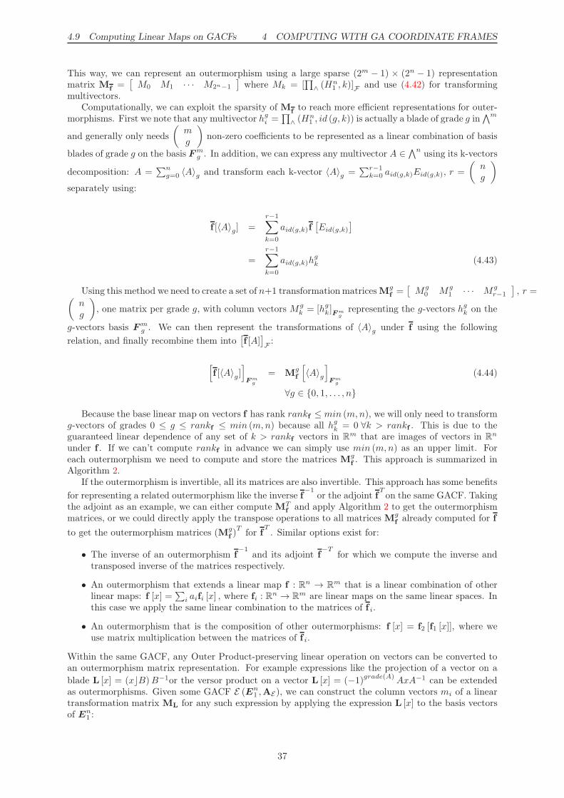
4.9 Computing Linear Maps on GACFs 4 COMPUTING WITH GA COORDINATE FRAMES

This way, we can represent an outermorphism using a large sparse (2m − 1) × (2n − 1) representationmatrix M

f=[M0 M1 · · · M2n−1

]where Mk = [

∏∧(Hn

1 , k)]F and use (4.42) for transformingmultivectors.

Computationally, we can exploit the sparsity of Mf

to reach more efficient representations for outer-morphisms. First we note that any multivector hg

i =∏

∧(Hn

1 , id (g, k)) is actually a blade of grade g in∧m

and generally only needs(

m

g

)non-zero coefficients to be represented as a linear combination of basis

blades of grade g on the basis Fmg . In addition, we can express any multivector A ∈

∧n using its k-vectors

decomposition: A =∑n

g=0 〈A〉g and transform each k-vector 〈A〉g =∑r−1

k=0 aid(g,k)Eid(g,k), r =

(n

g

)

separately using:

f [〈A〉g] =

r−1∑

k=0

aid(g,k)f[Eid(g,k)

]

=

r−1∑

k=0

aid(g,k)hgk (4.43)

Using this method we need to create a set of n+1 transformation matrices Mgf=[M

g0 M

g1 · · · M

gr−1

], r =(

n

g

), one matrix per grade g, with column vectors M

gk = [hg

k]Fmg

representing the g-vectors hgk on the

g-vectors basis Fmg . We can then represent the transformations of 〈A〉g under f using the following

relation, and finally recombine them into[f [A]

]F

:

[f [〈A〉g]

]Fm

g

= Mgf

[〈A〉g

]Fm

g

(4.44)

∀g ∈ {0, 1, . . . , n}

Because the base linear map on vectors f has rank rankf ≤ min (m,n), we will only need to transformg-vectors of grades 0 ≤ g ≤ rankf ≤ min (m,n) because all hg

k = 0 ∀k > rankf . This is due to theguaranteed linear dependence of any set of k > rankf vectors in Rm that are images of vectors in Rn

under f . If we can’t compute rankf in advance we can simply use min (m,n) as an upper limit. Foreach outermorphism we need to compute and store the matrices M

gf. This approach is summarized in

Algorithm 2.If the outermorphism is invertible, all its matrices are also invertible. This approach has some benefits

for representing a related outermorphism like the inverse f−1

or the adjoint fTon the same GACF. Taking

the adjoint as an example, we can either compute MTf

and apply Algorithm 2 to get the outermorphismmatrices, or we could directly apply the transpose operations to all matrices M

gf

already computed for f

to get the outermorphism matrices (Mgf)T for f

T. Similar options exist for:

• The inverse of an outermorphism f−1

and its adjoint f−T

for which we compute the inverse andtransposed inverse of the matrices respectively.

• An outermorphism that extends a linear map f : Rn → Rm that is a linear combination of otherlinear maps: f [x] =

∑i aifi [x] , where fi : R

n → Rm are linear maps on the same linear spaces. Inthis case we apply the same linear combination to the matrices of f i.

• An outermorphism that is the composition of other outermorphisms: f [x] = f2 [f1 [x]], where weuse matrix multiplication between the matrices of f i.

Within the same GACF, any Outer Product-preserving linear operation on vectors can be converted toan outermorphism matrix representation. For example expressions like the projection of a vector on ablade L [x] = (x⌋B)B−1or the versor product on a vector L [x] = (−1)grade(A)

AxA−1 can be extendedas outermorphisms. Given some GACF E (En

1 ,AE), we can construct the column vectors mi of a lineartransformation matrix ML for any such expression by applying the expression L [x] to the basis vectorsof En

1 :

37

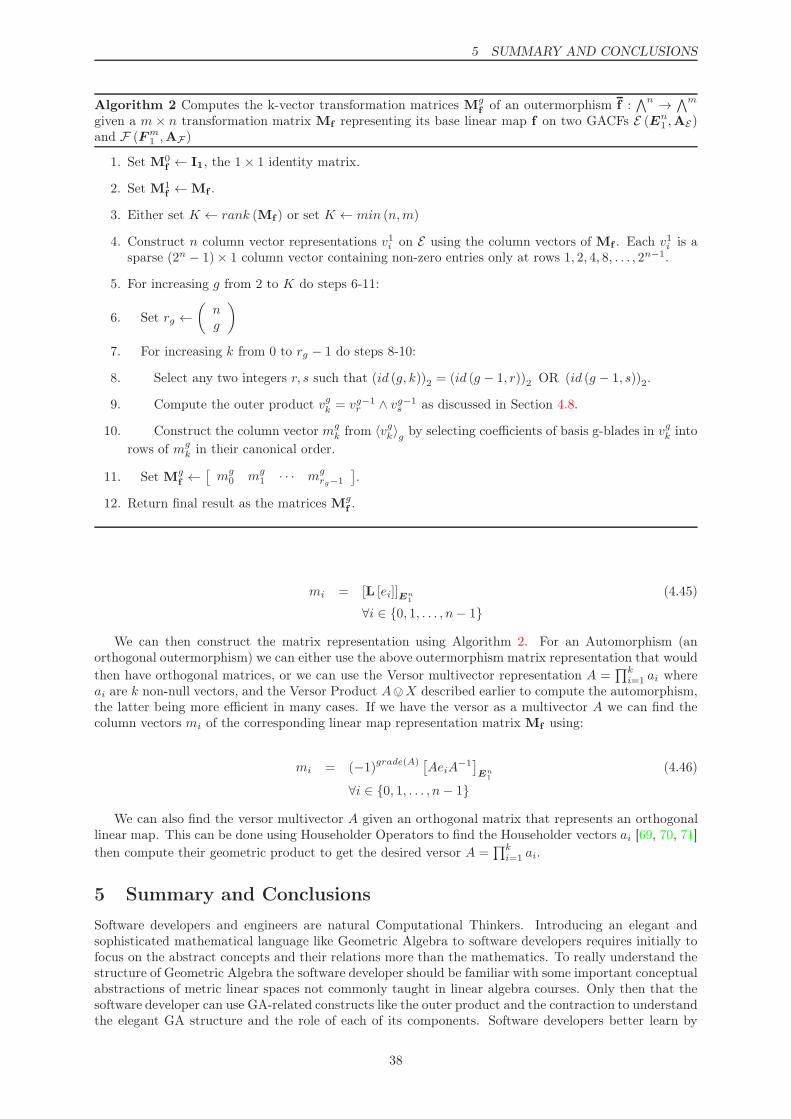
5 SUMMARY AND CONCLUSIONS

Algorithm 2 Computes the k-vector transformation matrices Mgf

of an outermorphism f :∧n →

∧m

given a m × n transformation matrix Mf representing its base linear map f on two GACFs E (En1 ,AE)

and F (Fm1 ,AF)

1. Set M0f← I1, the 1× 1 identity matrix.

2. Set M1f←Mf .

3. Either set K ← rank (Mf ) or set K ← min (n,m)

4. Construct n column vector representations v1i on E using the column vectors of Mf . Each v1i is asparse (2n − 1)× 1 column vector containing non-zero entries only at rows 1, 2, 4, 8, . . . , 2n−1.

5. For increasing g from 2 to K do steps 6-11:

6. Set rg ←

(n

g

)

7. For increasing k from 0 to rg − 1 do steps 8-10:

8. Select any two integers r, s such that (id (g, k))2 = (id (g − 1, r))2 OR (id (g − 1, s))2.

9. Compute the outer product vgk = vg−1

r ∧ vg−1s as discussed in Section 4.8.

10. Construct the column vector mgk from 〈vgk〉g by selecting coefficients of basis g-blades in v

gk into

rows of mgk in their canonical order.

11. Set Mgf←[m

g0 m

g1 · · · m

grg−1

].

12. Return final result as the matrices Mgf.

mi = [L [ei]]En1

(4.45)

∀i ∈ {0, 1, . . . , n− 1}

We can then construct the matrix representation using Algorithm 2. For an Automorphism (anorthogonal outermorphism) we can either use the above outermorphism matrix representation that wouldthen have orthogonal matrices, or we can use the Versor multivector representation A =

∏ki=1 ai where

ai are k non-null vectors, and the Versor Product A>X described earlier to compute the automorphism,the latter being more efficient in many cases. If we have the versor as a multivector A we can find thecolumn vectors mi of the corresponding linear map representation matrix Mf using:

mi = (−1)grade(A) [AeiA

−1]En

1

(4.46)

∀i ∈ {0, 1, . . . , n− 1}

We can also find the versor multivector A given an orthogonal matrix that represents an orthogonallinear map. This can be done using Householder Operators to find the Householder vectors ai [69, 70, 71]then compute their geometric product to get the desired versor A =

∏ki=1 ai.

5 Summary and Conclusions

Software developers and engineers are natural Computational Thinkers. Introducing an elegant andsophisticated mathematical language like Geometric Algebra to software developers requires initially tofocus on the abstract concepts and their relations more than the mathematics. To really understand thestructure of Geometric Algebra the software developer should be familiar with some important conceptualabstractions of metric linear spaces not commonly taught in linear algebra courses. Only then that thesoftware developer can use GA-related constructs like the outer product and the contraction to understandthe elegant GA structure and the role of each of its components. Software developers better learn by

38

REFERENCES REFERENCES

doing; they need to watch abstract mathematical ideas come to life on computer displays. Creating aGA-based software library is the best way for a software developer to learn the mathematical details ofGA. This article provided a Computational Thinking-based introduction to Geometric Algebra targetingsoftware developers. The main three parts of this article introduced concepts of metric linear systems,and then used them to construct the main structural elements of GA in the second part. The third partaimed at providing enough mathematics to implement a GA-based software library either for learning,prototyping, or production purposes. In addition, the interested reader can find enough resources in thereferences for more information on the concepts and techniques presented in this article.

I believe the future of widely accepting GA as a universal mathematical language for Geometric Com-puting depends on how the scientific computing and software engineering communities appreciate GA asa powerful language for developing Geometric Computing software systems. Making GA implementationsinto valuable and enjoyable software systems for the public domain is possible only through the efforts ofgood software developers who understand and use GA in their own creative Computational Thinking way.Targeting these communities should be a top priority for the GA community to gain more popularityfor their GA-based models. I recommend for the GA community to communicate more with softwaredevelopers on both academic and practical levels. This would also make the GA community more awareof the practical problems facing GA-based software implementations that would require more researchinto GA-based algorithms and techniques.

References

[1] D. Hestenes and G. Sobczyk, Clifford algebra to geometric calculus: A unified language for math-ematics and physics, ser. Fundamental theories of physics. Dordrecht and Boston and Hingham,MA, U.S.A.: D. Reidel and Distributed in the U.S.A. and Canada by Kluwer Academic Publishers,1984. 1, 3.4

[2] D. Hestenes, New Foundations for Classical Mechanics, 2nd ed., ser. Fundamental theories of physics.Dordrecht: Springer Netherlands, 2002, vol. 99. 1

[3] L. Dorst, D. Fontijne, and S. Manning, Geometric algebra for computer science: An object-orientedapproach to geometry, 2nd ed., ser. The Morgan Kaufmann series in computer graphics. Amsterdam[u.a.]: Morgan Kaufmann/Elsevier, 2009. 1, 1.1, 1.2, 2.7, 3, 3.1, 3.2, 3.2, 3.3, 3.3, 3.6, 3.8, 3.8, 4, 4.7

[4] G. Sommer, Geometric computing with Clifford algebras: Theoretical foundations and applicationsin computer vision and robotics. Berlin and New York: Springer, 2001. 1, 1.2

[5] G. Sobczyk, “Clifford geometric algebras in multilinear algebra and non-euclidean geometries,” inNATO Science Series II: Mathematics, Physics and Chemistry. Kluwer Academic Publishers, 2004,pp. 1–27. 1, 1.2

[6] C. Doran and A. Lasenby, Geometric Algebra for Physicists. Cambridge University Press, 2007. 1,1.2

[7] C. Gunn, “Geometric algebras for euclidean geometry,” Advances in Applied Clifford Algebras, 2016.1, 1.2, 2.7

[8] M. Nilsson, “Geometric algebra with conzilla: Building a conceptual web of mathematics,” MSc,Center for User-Oriented IT-design, Royal Institute of Technology, Stockholm, 2002. [Online].Available: http://cid.nada.kth.se/pdf/CID-201.pdf 1, 1.2

[9] J. M. Pozo and G. Sobczyk, “Geometric algebra in linear algebra and geometry,” Acta ApplicandaeMathematicae, vol. 71, no. 3, pp. 207–244, 2002. 1

[10] C. Perwass, Geometric algebra with applications in engineering, ser. Geometry and computing.Berlin: Springer, 2009, vol. 4. 1, 2.7, 3, 3.3, 3.5, 3.8

[11] D. Lundholm and L. Svensson, “Clifford algebra, geometric algebra, and applications.” [Online].Available: http://arxiv.org/pdf/0907.5356 1, 2.1

[12] L. Dorst, “Tutorial: Structure-preserving representation of euclidean motions through conformalgeometric algebra,” in Geometric algebra computing, E. Bayro Corrochano and G. Scheuermann,Eds. London: Springer, 2010, pp. 35–52. 1

39

REFERENCES REFERENCES

[13] L. Dorst and J. Lasenby, Eds., Guide to geometric algebra in practice. London and New York:Springer, 2011. 1

[14] A. Macdonald, Linear and Geometric Algebra. CreateSpace Independent Publishing Platform, 2011.1, 3

[15] E. Chisolm, “Geometric algebra.” [Online]. Available: http://arxiv.org/pdf/1205.5935 1

[16] E. Hitzer, T. Nitta, and Y. Kuroe, “Applications of clifford’s geometric algebra,” Advances in AppliedClifford Algebras, vol. 23, no. 2, pp. 377–404, mar 2013. 1

[17] J. M. Chappell, S. P. Drake, C. L. Seidel, L. J. Gunn, A. Iqbal, A. Allison, and D. Abbott, “Geometricalgebra for electrical and electronic engineers,” Proceedings of the IEEE, vol. 102, no. 9, pp. 1340–1363, 2014. 1, 1.2

[18] K. Kanatani, Understanding Geometric Algebra: Hamilton, Grassmann, and Clifford for ComputerVision and Graphics. CRC Press, 2015. 1, 2.7, 3, 3.1

[19] A. Macdonald, “A survey of geometric algebra and geometric calculus,” Advances in Applied CliffordAlgebras, vol. 27, no. 1, pp. 853–891, apr 2017. 1

[20] M. D. Zaharia and L. Dorst, “The interface specification and implementation internals of a programmodule for geometric algebra.” 1, 3.8, 4

[21] D. Fontijne, Efficient implementation of geometric algebra. [S.l. and Amsterdam: s.n.] and Univer-siteit van Amsterdam [Host], 2007. 1, 4

[22] D. Hildenbrand, Foundations of geometric algebra computing, ser. Geometry and computing. Hei-delberg and New York: Springer, 2013, vol. v. 8. 1, 2.7, 3

[23] R. Abłamowicz and B. Fauser, “On parallelizing the clifford algebra product for CLIFFORD,” Ad-vances in Applied Clifford Algebras, vol. 24, no. 2, pp. 553–567, feb 2014. 1

[24] W. Luo, Y. Hu, Z. Yu, L. Yuan, and G. Lü, “A hierarchical representation and computation schemeof arbitrary-dimensional geometrical primitives based on cga,” Advances in Applied Clifford Algebras,2016. 1

[25] D. Hildenbrand, J. Albert, P. Charrier, and C. Steinmetz, “Geometric algebra computing for het-erogeneous systems,” Advances in Applied Clifford Algebras, vol. 27, no. 1, pp. 599–620, jun 2016.1

[26] S. Breuils, V. Nozick, and L. Fuchs, “A geometric algebra implementation using binary tree,” Ad-vances in Applied Clifford Algebras, vol. 1, p. 350, 2017. 1

[27] W. Benger and W. Dobler, “Massive geometric algebra: Visions for c++ implementations of ge-ometric algebra to scale into the big data era,” Advances in Applied Clifford Algebras, apr 2017.1

[28] S. Ghali, Introduction to Geometric Computing. Springer London, 2008. 1.1

[29] K. Mehlhorn and S. Naher, Leda. Cambridge University Press, 1999. 1.1

[30] D.-Z. Du and F. K. Hwang, Computing in Euclidean Geometry (2nd Edition). WORLD SCIEN-TIFIC PUB CO INC, 1995. 1.1

[31] P. J. Denning, D. E. Comer, D. Gries, M. C. Mulder, A. Tucker, A. J. Turner, and P. R. Young,“Computing as a discipline,” Communications of the ACM, vol. 32, no. 1, pp. 9–23, 1989. 1.1

[32] D. Jackson, Software abstractions: Logic, language, and analysis / Daniel Jackson, revised edition ed.Cambridge, Mass.: MIT Press, 2012. 1.1

[33] A. M. K., Computer Graphics And Geometric Modeling: Mathematics. Eswar Press, 2010. 1.1

[34] ——, Computer Graphics And Geometric Modeling: Implementation And Algorithms. SpringerIndia, 2010. 1.1

40

REFERENCES REFERENCES

[35] R. Goldman, An Integrated Introduction to Computer Graphics and Geometric Modeling. Taylor &Francis Inc, 2009. 1.1, 2.2, 3.1

[36] C. Gunn, “Geometry, kinematics, and rigid body mechanics in cayley-klein geometries,” phdthesis,Technische UniversitÀt Berlin, FakultÀt II - Mathematik und Naturwissenschaften, 2011. 1.1,2.5, 2.7

[37] L. Yuan, Z. Yu, W. Luo, L. Yi, and G. LÃŒ, “Geometric algebra for multidimension-unified geo-graphical information system,” Advances in Applied Clifford Algebras, vol. 23, no. 2, pp. 497–518,oct 2012. 1.1

[38] J. M. Chappell, A. Iqbal, J. G. Hartnett, and D. Abbott, “The vector algebra war: A historicalperspective,” IEEE Access, vol. 4, pp. 1997–2004, 2016. 1.1, 3.1

[39] D. Hestenes, “The genesis of geometric algebra: A personal retrospective,” Advances in AppliedClifford Algebras, vol. 27, no. 1, pp. 351–379, 2017. 1.1, 2.1

[40] B. Kules, “Computational thinking is critical thinking: Connecting to university discourse, goals, andlearning outcomes,” Proceedings of the Association for Information Science and Technology, vol. 53,no. 1, pp. 1–6, 2016. 1.2

[41] C. Selby and J. Woollard, “Refining an understanding of computational thinking,” Author’s original,pp. 1–23, 2014. 1.2

[42] J. M. Wing, “Computational thinking,” Communications of the ACM, vol. 49, no. 3, p. 33, 2006. 1.2

[43] A. L. Onishchik and R. Sulanke, Projective and Cayley-Klein Geometries. Springer Berlin Heidel-berg, 2006. 1, 2.6

[44] J. Richter-Gebert, Perspectives on Projective Geometry. Springer-Verlag GmbH, 2011. 1, 1.2, 2.5

[45] C. Coronel and S. Morris, Database Systems: Design, Implementation, & Management. COURSETECHNOLOGY, 2016. 1.2

[46] R. Wang, Introduction to orthogonal transforms: With applications in data processing and analysis/ by Ruye Wang. Cambridge: Cambridge University Press, 2011. 1.2

[47] E. Bayro Corrochano and G. Scheuermann, Eds., Geometric algebra computing: In engineering andcomputer science / edited by Eduardo Bayro-Corrochano, Gerik Scheuermann. London: Springer,2010. 1.2

[48] E. Hitzer, “The quest for conformal geometric algebra fourier transformations,” in AIP ConferenceProceedings 1558, 529 (2013), ser. AIP Conference Proceedings. AIP, 2013, pp. 529–532. 1.2

[49] E. M. S. Hitzer and L. Redaelli, “Geometric algebra illustrated by cinderella,” Advances in AppliedClifford Algebras, vol. 13, no. 2, pp. 157–181, oct 2003. 1.2

[50] J. Richter-Gebert and U. Kortenkamp. [Online]. Available: https://www.cinderella.de 1.2

[51] D. Goldberg, “What every computer scientist should know about floating-point arithmetic,”ACM Computing Surveys, vol. 23, no. 1, pp. 5–48, mar 1991. [Online]. Available:https://docs.oracle.com/cd/E19957-01/806-3568/ncg_goldberg.html 1.2

[52] D. S. Dummit and R. M. Foote, Abstract Algebra. JOHN WILEY & SONS INC, 2003. 1.2, 2.1

[53] J. S. Golan, The Linear Algebra a Beginning Graduate Student Ought to Know. Springer Nether-lands, 2007. 1.2, 2.2

[54] S. J. Axler, Linear algebra done right, 3rd ed., ser. Undergraduate texts in mathematics. New York:Springer, 2015. 1.2, 2.2

[55] D. Poole, Linear algebra: A modern introduction, 4th ed. Stamford CT: Cengage Learning, 2015.1.2, 2.2, 2.3

[56] M. L. Scott, Programming Language Pragmatics, 3rd ed. Morgan Kaufmann, 2009. 1.2

41

REFERENCES REFERENCES

[57] M. Gabbrielli and S. Martini, Programming Languages: Principles and Paradigms. Springer-VerlagGmbH, 2010. 1.2

[58] A. H. Eid, “Optimized automatic code generation for geometric algebra based algorithms with raytracing application,” phdthesis, Faculty of Engineering, Port-Said University, Egypt, Apr. 2010.[Online]. Available: http://arxiv.org/pdf/1607.04767 1.3, 4

[59] ——. [Online]. Available: https://gacomputing.info/about-gmac/ 1.3, 4

[60] R. Lidl, Introduction to Finite Fields and Their Applications. CAMBRIDGE UNIV PR, 2002. 2.1

[61] G. L. Mullen and D. Panario, Handbook of Finite Fields. Taylor & Francis Ltd, 2013. 2.1

[62] L. Aveneau, L. Fuchs, and E. Andres, “Digital geometry from a geometric algebra perspective,” inDiscrete Geometry for Computer Imagery. Springer International Publishing, 2014, pp. 358–369.2.1

[63] H. Tuy, Convex Analysis and Global Optimization. Springer International Publishing, 2016. 2.2

[64] S. J. Sangwine and E. Hitzer, “Clifford multivector toolbox (for MATLAB),” Advances in AppliedClifford Algebras, vol. 27, no. 1, pp. 539–558, apr 2016. 2.3, 3.5

[65] ——. [Online]. Available: http://clifford-multivector-toolbox.sourceforge.net/ 2.3

[66] S. Roman, Advanced Linear Algebra. Springer New York, 2007. 2.4

[67] I. R. Shafarevich and A. O. Remizov, Linear Algebra and Geometry. Springer Berlin Heidelberg,2013. 2.5, 2.6

[68] I. Gohberg, P. Lancaster, and L. Rodman, Invariant Subspaces of Matrices with Applications (Clas-sics in Applied Mathematics). SIAM, Society for Industrial and Applied Mathematics, 2006. 2.5

[69] T. A. Davis, Direct Methods for Sparse Linear Systems. Society for Industrial and Applied Math-ematics, jan 2006. 2.5, 4.9

[70] W. H. PRESS, NUMERICAL RECIPES. CAMBRIDGE UNIVERSITY PRESS, 2007. 2.5, 4.9

[71] T. B. Co, Methods of Applied Mathematics for Engineers and Scientists. Cambridge UniversityPress, 2013. 2.5, 4.9

[72] G. Strang, “The fundamental theorem of linear algebra,” The American Mathematical Monthly, vol.100, no. 9, p. 848, nov 1993. 2.5

[73] D. Timashev, Homogeneous Spaces and Equivariant Embeddings. Springer Berlin Heidelberg, 2011.2.7

[74] D. Hestenes, Space-Time Algebra. Springer International Publishing, 2015. 2.7

[75] J. Dressel, K. Y. Bliokh, and F. Nori, “Spacetime algebra as a powerful tool for electromagnetism,”Physics Reports, vol. 589, pp. 1–71, aug 2015. 2.7

[76] C. B. Perwass and D. Hildenbrand, “Aspects of geometric algebra in euclidean, projective and con-formal space: An introductory tutorial.” 2.7

[77] R. Goldman, S. Mann, and X. Jia, “Computing perspective projections in 3-dimensions using rotorsin the homogeneous and conformal models of clifford algebra,” Advances in Applied Clifford Algebras,vol. 24, no. 2, pp. 465–491, jan 2014. 2.7

[78] C. Gunn, “On the homogeneous model of euclidean geometry,” in Guide to geometric algebra inpractice, L. Dorst and J. Lasenby, Eds. London and New York: Springer, 2011, pp. 297–327. 2.7

[79] C. G. Gunn, “Doing euclidean plane geometry using projective geometric algebra,” Advances inApplied Clifford Algebras, 2016. 2.7

[80] R. B. Easter and E. Hitzer, “Double conformal geometric algebra,” Advances in Applied CliffordAlgebras, apr 2017. 2.7

42

REFERENCES REFERENCES

[81] D. Klawitter, “A clifford algebraic approach to line geometry,” Advances in Applied Clifford Algebras,vol. 24, no. 3, pp. 713–736, apr 2014. 2.7

[82] R. Goldman and S. Mann, “R(4, 4) as a computational framework for 3-dimensional computergraphics,” Advances in Applied Clifford Algebras, vol. 25, no. 1, pp. 113–149, 2015. 2.7

[83] L. Dorst, “3d oriented projective geometry through versors of r(3,3),” Advances in Applied CliffordAlgebras, 2015. 2.7

[84] D. Klawitter, “Reflections in conics, quadrics and hyperquadrics via clifford algebra,” Beiträge zurAlgebra und Geometrie / Contributions to Algebra and Geometry, vol. 57, no. 1, pp. 221–242, 2016.2.7

[85] C. Perwass. [Online]. Available: https://www.raytrix.de/downloads/ 3

[86] L. Dorst, “The inner products of geometric algebra,” in Applications of geometric algebra in computerscience and engineering, L. Dorst, C. Doran, and J. Lasenby, Eds. Boston: Birkhäuser, 2002, pp.35–46. 3.2, 3.2

[87] P. Lounesto, “Marcel riesz’s work on clifford algebras,” in Clifford Numbers and Spinors. SpringerNetherlands, 1993, pp. 246–247. 3.2

[88] J. Gallier, Geometric Methods and Applications. Springer New York, 2001. 3.7

[89] L. C. Grove, Classical Groups and Geometric Algebra (Graduate Studies in Mathematics). AmericanMathematical Society, 2001. 3.7

[90] T. A. Bouma, L. Dorst, and H. G. J. Pijls, “Geometric algebra for subspace operations,” ActaApplicandae Mathematicae, vol. 73, no. 3, pp. 285–300, 2002. 3.8

[91] D. Fontijne and L. Dorst, “Efficient algorithms for factorization and join of blades,” in GeometricAlgebra Computing. Springer London, 2010, pp. 457–476. 3.8

43