aij guidelines for practical applications of cfd to...
TRANSCRIPT

AIJ Guidelines for Practical Applications of CFD to Pedestrian Wind Environment around Buildings
Yoshihide Tominagaa* Akashi Mochidab, Ryuichiro Yoshiec, Hiroto Kataokad, Tsuyoshi Nozue,
Masaru Yoshikawaf, Taichi Shirasawac
aNiigata Institute of Technology, Fujihashi 1719, Kashiwazaki-City, Niigata, Japan bTohoku University, Aoba 06, Aramaki, Aoba-ku, Sendai-City, Miyagi, Japan cTokyo Polytechnic University, Iiyama 1583, Atsugi-City, Kanagawa, Japan
dTechnical Research Institute, Obayashi Corp., Shimokiyoto 4-640, Kiyose-City, Tokyo, Japan eInstitute of Technology, Shimizu Corp., Echujima 3-4-17, Koto-ku, Tokyo, Japan fTechnology Center, Taisei Corp., Nasecho 344-1, Totsuka-ku, Yokohama, Japan
ABSTRACT Significant improvements of computer facilities and Computational Fluid Dynamics (CFD) software in recent years have enabled prediction and assessment of the pedestrian wind environment around buildings in the design stage. Therefore, guidelines are required that summarize important points in using the CFD technique for this purpose. This paper describes guidelines proposed by the Working Group of the Architectural Institute of Japan (AIJ). The feature of these guidelines is that they are based on cross comparison between CFD predictions, wind tunnel test results and field measurements for seven test cases used to investigate the influence of many kinds of computational conditions for various flow fields. Keywords: CFD, Pedestrian wind environment, Prediction, Guidelines, Benchmark test 1 INTRODUCTION
Significant improvements of computer facilities and Computational Fluid Dynamics (CFD) software in recent years have enabled prediction and assessment of the pedestrian wind environment around buildings in the design stage. However, CFD has been applied with insufficient information about the influence of many factors related to the computational condition on prediction results. There have been several case studies on the pedestrian level wind environment around actual buildings using CFD (Stathopoulos and Baskaran, 1996; Timofeyef, 1998; Westbury et al., 2002 ; Richards et al, 2002). However, the influence of the computational conditions, i.e., grid discretization, domain sizes, boundary conditions, etc., on the prediction accuracy have not been systematically investigated. Therefore, a set of guidelines is required that summarize important points in using the CFD technique for appropriate prediction of pedestrian wind environment.
Some guidelines on industrial CFD applications have been published in order to clarify the method for validation and verification of CFD results (Roache et al., 1986; AIAA, 1998; ERCOFTAC, 2000). These guidelines provide valuable information on the applications for flow around buildings. However, no guidelines have yet been established on the use of CFD for investigating the pedestrian wind environment around buildings.
Recommendations have recently been proposed on the use of CFD in predicting the pedestrian wind environment by COST (European Cooperation in the field of Scientific and Technical Research) group (Action C14“Impact of Wind and Storms on City Life and Built Environment” Working Group 2 – CFD techniques). These recommendations (hereafter COST) were mainly based on the results published by other authors. They are summarized by Franke et al. (2004) and Franke (2006).
The guidelines for CFD prediction of the pedestrian wind environment around buildings were proposed by the Working Group in the Architectural Institute of Japan (AIJ), which consists of researchers from several universities and private companies. This working group conducted a lot of wind tunnel experiments, field measurements and the computations using different CFD codes to investigate the influence of various kinds of computational parameters for various flow fields. A distinctive feature of these guidelines is that they were derived from extensive and numerous cross comparisons, while those proposed by COST mainly consist of results obtained from a literature review. This paper also discusses similarities and differences to the COST recommendations.
The guidelines proposed here are mainly based on high Reynolds (Re) number RANS (Reynolds Averaged Navier-Stokes equations) models, although it is desirable to use a Large Eddy Simulation (LES) and a low Re number type model in order to obtain more accurate results. However, it is difficult to use those models for practical analysis because many computational cases and a huge number of grids are required for the prediction and analysis of the pedestrian wind environment under severe time restrictions. In spite of that, these guidelines can also be helpful when using a highly accurate model like an LES or low Re number type model. 2 OUTLINE OF CROSS COMPARISON TESTS
In order to clarify the major factors affecting prediction accuracy, the Working Group carried out cross comparisons of wind tunnel experiments, field measurements and CFD results of flow around a single high-rise building placed within the surface boundary layer, flow within a building complex in an actual urban area, and flow around a tree, obtained from various k-ε models, DSM and LES. Fig.1 illustrates seven test cases for these cross comparisons. In order to assess the effect of a specific factor, e.g., the performance of a turbulence model, the results were compared under the same computational conditions as for other factors. Special attention was paid to this point in this project. The basic computational conditions, i.e., grid arrangements, boundary conditions, etc., were specified by the organizers. Contributors were requested to use these conditions. The results of these cross comparisons have been reported in several papers (Mochida et al., 2002; Shirasawa et al., 2003; Tominaga et al., 2004; Yoshie et al., 2005a, Yoshie et al., 2005b; Tominaga et al., 2005; Yoshie et al., 2006, Mochida et al. 2006)). 3 COMPUTATIONAL DOMAIN AND REPRESENTATION OF SURROUNDINGS 3.1 Domain size
For the size of the computational domain, the blockage ratio should be below 3% based on knowledge of wind tunnel experiments. For the single building model, the lateral and the top boundary should be set 5H or more away from the building, where H is the height of the target building (Mochida et al., 2002; Shirasawa et al., 2003). The distance between the inlet boundary and the building should be set to correspond to the upwind area covered by a smooth floor in the wind tunnel. The outflow boundary should be set at least 10H behind the building. Where the building surroundings are included, the height of the computational domain should be set to correspond to the boundary layer height determined by the terrain category of the surroundings (AIJ, 2004). The lateral size of the computational domain should extend about 5H from the outer edges of the target building and the buildings included in the computational domain should not exceed the recommended blockage ratio (3%).
Similar requirements for the inlet and the top boundaries were suggested by COST. However, the recommend lateral boundaries (2.3W, where W is width of built area) and the outflow boundaries

(15Hmax, where Hmax is the height of the tallest building) (Franke, 2006) may be conservative. It should be noted that there is a possibility of unrealistic results if the computational region is expanded without representation of surroundings (Yoshie et al. 2006). 3. 2 Representation of surroundings
For the actual urban area, the buildings in the region to be assessed (generally 1-2H radius from the target building) should be clearly modeled. Moreover, at least one additional street block in each direction around the assessment region should also be clearly reproduced (Yoshie et al., 2005a; Yoshie et al., 2005b). In addition, it is recommended to use some simplified geometries of a cluster of buildings or to specify appropriate roughness lengths zo for the ground surface boundary condition to represent the roughness of the outer region (from the outer edge of the additional street blocks to the boundary of the computational domain).
COST suggest that the central building, at which wind effects are of main interest, requires the greatest level of detail but its area and resolutions to be represented have not been mentioned (Franke, 2006). 3.3 Treatment of obstacle smaller than grid size
To simulate the aerodynamic effects of small scale obstacles such as small buildings, sign boards, trees and moving automobiles, etc., it is necessary to add additional terms to the basic flow equations in order to decrease wind velocity but increase turbulence. This is called a canopy model and is based on the k-ε model in which extra terms are added to the transport equations. These extra terms are derived by applying the spatial average to the basic equations (Hiraoka, 1993; Maruyama, 1993; Hataya et al., 2006). A volume fraction technique, e.g. FAVOR (Hirt et al., 1993), is a simplified technique for considering the effect of an obstacle smaller than the grid.
In particular, tree planting is one of the most popular measures for improving the pedestrian wind environment. Mochida et al. (2006) has classified various tree canopy models and have also compared the predictions of various canopy models with field measurements of flows around trees. It is suggested that users should compare their results with Mochida et al. (2006) when any kind of tree canopy model is used. 4 GRID DISCRETIZATION 4.1 General notice
In order to predict the flow field around a building with acceptable accuracy, the most important thing is to correctly reproduce the characteristics of separating flows near the roof and the walls. Therefore, a fine grid arrangement is required to resolve the flows near the corners. However, it is generally very difficult to resolve the viscous sub-layers near the building walls and it is also difficult to adopt no-slip boundary conditions on the walls. The use of wall functions to represent flow around buildings is basically incorrect, since many wall functions such as logarithmic laws have been developed considering the situations in the attached boundary-layer flows. However, many buildings are bluff bodies with sharp edges and separating points are always found at the leading edges, regardless of the Re numbers. In such cases, the decrease of accuracy due to the use of wall functions is not as significant as expected.
According to cross comparisons results for a simple building model (Mochida et al., 2002; Shirasawa et al., 2003, Yoshie et.al., 2005a), the minimum of ten grids is required on one side of a building to

reproduce the separation flow around the upwind corners. Grid shapes should be set up so that the widths of adjacent grids are similar, especially in regions
with a steep velocity gradient. In these regions, it is desirable to set a stretching ratio of adjacent grids of 1.3 or less. However, it is desirable to confirm that the results would not change with different grid layouts, since these recommended stretching ratios may change according to the shape of the building and its surroundings.
COST advises the same limitation for grid stretching ratio, and it recommends that the sensitivity of the results on mesh resolution should be tested (Franke et al., 2004). 4.2 Grid resolution for actual building complex
The minimum grid resolution should be set to about 1/10 of the building scale (about 0.5-5.0m) within the region including the evaluation points around the target building. Moreover, the grids should be arranged so that the evaluation height (1.5-5.0m above ground) is located at the 3rd or higher grid from the ground surface (Yoshie et al., 2005a; Tominaga et al. 2005).
COST suggests that at least ten cells should be used per building side and ten cells per cube root of building volume as an initial choice. It also recommends that pedestrian wind speeds at 1.5m - 2m high be calculated at the third or fourth cell above ground (Franke et al., 2004). Those requirements are comparable with the AIJ guidelines. 4.3 Grid dependence of solution
It should be confirmed that the prediction result does not change significantly with different grid systems. The number of fine meshes should be at least 1.5 times the number of coarse meshes in each dimension (Ferziger and Peric, 2002).
COST indicates that at least three systematically and substantially refined grids should be used so that the ratio of cells for two consecutive grids should be at least 3.4 (Franke et al., 2004). The value of 3.4 means finer girds with 1.5 times the grid number in three dimensions, i.e., 1.53=3.375.
4.4 Unstructured Grid
It is necessary to ensure that the aspect ratios of the grid shapes do not become excessive in regions adjacent to coarse girds or near the surfaces of complicated geometries. For improved accuracy, it is desirable to arrange the boundary layer elements (prismatic cells) parallel to the walls or the ground surfaces (Fig. 2). COST also introduces the same technique. 5 BOUNDARY CONDITIONS 5.1 Inflow boundary condition
The vertical velocity profile U(z) on flat terrain is usually given by a power law (AIJ, 2004). α
⎟⎟⎠
⎞⎜⎜⎝
⎛=
sS z
zUzU )( (5)
SU :Velocity at reference height, Sz α : power-law exponent determined by terrain category
The vertical distribution of turbulent energy k(z) can be obtained from a wind tunnel experiment or a observation of corresponding surroundings. If it is not available, k(z) can be also given by Eqn. (6) based on the estimation equation for the vertical profile of turbulent intensity I(z) proposed by AIJ

Recommendations for Loads on Buildings (2004). ).α(
G
u
zz.
)z(U)z(σ)z(I
050
10−−
⎟⎟⎠
⎞⎜⎜⎝
⎛== (6)
zG : Boundary layer height determined by terrain category σu:R.M.S. value of velocity fluctuation in stream-wise direction.
In the atmospheric boundary layer, the following relation between I(z) and k(z) can be assumed.
22222
))()(()(2
)()()()( zUzIz
zzzzk u
wvu ⋅=≅++
= σσσσ
(7)
It is recommended that the values of ε are given by assuming local equilibrium of Pk = ε (Pk : Production term for k equation).
( ) ( ) ( ) ( ) ( )dz
zdUzkCdz
zdUz'w'uzP)z(ε /µk
21≅−≅≅ (8)
When the vertical gradient of velocity can be expressed by a power law with exponent α, ( 1)
1/ 2( ) ( ) s
s s
U zz C k zz z
α
µε α−
⎛ ⎞= ⎜ ⎟
⎝ ⎠ (9)
µC : model constant (= 0.09)
For the inflow boundary conditions, COST recommends the formulas suggested by Richards and Hoxey (1993), in which the vertical profiles for U(z), k(z) and ε(z) in the atmospheric boundary layer by assuming a constant shear stress with height are as follows.
*0( ) lnABL z zUU z
zκ+⎛ ⎞= ⎜ ⎟
⎝ ⎠ (10)
* 2
( ) ABLUk zCµ
= (11)
* 3
0
( )( )
ABLUzz z
εκ
=+
(12)
κ : Karman constant (= 0.4) *ABLU : atmospheric boundary layer friction velocity
*ABLU is calculated from a specified velocity Uh at reference height h as
*
0ln
hABL
UUh z
z
κ=
+⎛ ⎞⎜ ⎟⎝ ⎠
(13)
Uh : specified velocity at a reference height h The vertical profiles expressed in Eqns. (5)-(9) are given by assumimg the power-law exponent α,
and are consistent with the wind load estimation method in Japan (AIJ, 2004). However, the recommended profiles in COST, as described by Eqns. (10) - (13), are based on an assumed value of the roughness parameter z0. Eqns. (10) - (13) assume that the height of the computational domain is much lower than the atmospheric boundary layer height because the assumption of constant shear stresses is only valid in the lower part of the atmospheric boundary layer. Therefore, it is necessary to pay attention to the relationship between the height of the computational domain and the atmospheric boundary layer.

5.2 Lateral and upper surfaces of computational domain If the computational domain is large enough (see section 3.1), the boundary conditions for lateral and
upper surfaces do not have significant influences on the calculated results around the target building (Mochida et al., 2002; Shirasawa et al., 2003; Yoshie et al., 2005a). Using the inviscid wall condition (normal velocity component and normal gradients of tangential velocity components set to zero) with a large computational domain will make the computation more stable. 5.3 Downstream boundary
It is common to set the normal gradients of all variables to zero for the outflow boundary condition. The outflow boundary needs to be placed far from the region where the influence of the target building is negligible (see section 3.1). 5.4 Solid surface boundary conditions for velocities (1)Ground surface for Single building model for comparison with experimental result
When choosing the ground surface boundary conditions, the most important principle is that the computational trail of a simple boundary layer flow without a building should be firstly assessed. The vertical profile of wind velocity gradually changes near the turntable floor in a wind tunnel as the flow proceeds downstream. Boundary conditions that reproduce this gradual change in velocity profile should be used.
A logarithmic law for a smooth wall surface or a logarithmic law with roughness parameters z0 or kS (kS : sand-grain roughness height) can be used for the boundary condition.
The logarithmic law for a smooth wall surface is expressed as follows.
( )( )1/ 2
1/ 2
/1 1ln ln/
w PPn
w
zUz A A
vτ ρ
κ κτ ρ+ ⋅
= + = + (14)
PU :tangential component of velocity vector at near-wall node wτ : shear stress at the wall, nz + : wall unit
Pz :distance between the definition point of PU and wall A: universal constant (=5~5.5)
To obtain wτ without iterative calculation, one can use its generalized form proposed by Launder and Spalding (1974). Murakami and Mochida (1988) have applied this generalized log-law boundary conditions to investigate flows around a building.
The logarithmic law with roughness parameter z0 is expressed as follows.
1/ 20
1 ln( / )
P P
w
U zzτ ρ κ
⎛ ⎞= ⎜ ⎟
⎝ ⎠ (15)
If the boundary layer formed near the ground can be regarded as the constant flux layer, the value of z0 can be assumed from the logarithmic law using the relation 1/ 2 1/ 4 1/ 2( / ) *w U C kµτ ρ = = and the measured values of velocity and k near the ground surface.
⎟⎟
⎠
⎞
⎜⎜
⎝
⎛=
2/14/1
0
expP
P
P
kCU
zz
µ
κ (16)
Pk : k value at Pz

In order to check whether the given boundary condition is appropriate, it should be confirmed that the velocity profile near the ground surface is similar to wind tunnel observations at a few measured locations. This can be done by 2D computation of boundary layer flow with the same grids in the vertical plane of the 3D grid system. It was thus confirmed that the condition with Eqns. (15) and (16) could minimize the changes in the vertical profiles obtained by Eqns. (5) - (9) for test case A (Mochida et al., 2002). COST also emphasizes verification of the assumption of an equilibrium boundary layer corresponding to the prescribed approach flow by performing a simulation in an empty domain with the same grid and boundary conditions as the final computation (Franke, 2006). (2)Ground surface for Actual Building Complex
The boundary condition corresponding to the actual ground surface should be used. For example, for a smooth ground surface, the logarithmic law for a smooth wall (Eqn. (14)) can be used.
For a rough ground surface, which can be expressed by a roughness length z0, a logarithmic law including a roughness parameter (Eqn. (15)) is applicable.
COST points out that the rough wall condition with kS leads to a very bad resolution of the flow close to the wall, because the first calculation node of the wall should be placed at least one kS away from the wall. Therefore, the use of the smooth wall condition for a built area is recommended (Franke et al, 2004). More detailed investigation was reported by Blocken et al (2007). (3)Building wall
For the building walls, the boundary condition according to the above principle is used. 5.5 Solid surface boundary for turbulent energy k and dissipation rate ε (1) Turbulent energy k
The transport equation of k is solved with the condition that the normal gradient of k is zero. (2) Dissipation rate ε
The dissipation rate ε at the first grid point, εP is given by 3/ 4 3/ 2
PP
P
C kz
µεκ
= (17)
6 SOLUTION ALGORITHM, SPATIAL DISCRETIZATION 6.1 Solution algorithm
Basically, steady and unsteady calculations using the RANS model should result in the same solutions if unsteady fluctuation does not occur in the calculation and if both are sufficiently convergent. However, in real situations, unsteady periodic fluctuation usually occurs behind high-rise buildings. This fluctuation essentially differs from that of turbulence, and can not be reproduced by a steady calculation. This periodic fluctuation is not reproduced in many cases using a high Re number type k-ε model, although the unsteady calculation is conducted. It may be reproduced when highly accurate turbulence models and boundary conditions are used (Mochida et al., 2002; Tominaga et al., 2003). For this case, the time averaged values of each variable need to be calculated because the solution changes with time. 6.2 Scheme for convection terms
The first order upwind scheme is not appropriate for all transported quantities, since the spatial gradients of the quantities tend to become diffusive due to a large numerical viscosity.
COST also does not recommend the use of first order methods like the upwind scheme except in initial iterations (Franke et al., 2004).

7 CONVERGENCE OF SOLUTION 7.1 Criteria for convergence
Calculation needs to be finished after sufficient convergence of the solution. For this purpose, it is important to confirm that the solution does not change by monitoring the variables on specified points or by overlapping the contours among calculation results at different calculation steps. The default values for convergence in most commercial codes are not strict because code vendors want to stress calculation efficiency. Therefore, stricter convergence criteria are required to check that there is no change in the solution.
When the calculation diverges or convergence is slow, the points below should be examined. -The aspect ratio and the stretching ratio of the grids may be too large. -The relaxation coefficient of the matrix solver may be too small. -Periodic fluctuations such as a vortex shedding may be occurring. COST suggests that scaled residuals should be dropped 4 orders of magnitude (Franke, 2006).
However, these values are largely dependent on flow configuration and boundary conditions, so it is better to check the solution directly using different convergence criteria, as mentioned above. 7.2 Initial conditions
To obtain the converged solution quickly, an appropriate physical property of initial condition should be given. The inflow profiles extended to the whole domain or the results obtained by laminar flow computation are often used for the initial condition. 8 TURBULENCE MODELS
The well-known problem of the standard k-ε model is that it cannot reproduce the separation and reverse flow at the roof top of a building due to its overestimation of turbulence energy k at the impinging region of the building wall. Although this problem does not appear near the ground surface as much as it does on the roof, it may affect the prediction accuracy of the value and the location of high velocity. However, many revised k-ε models and DSM (Differential Stress Model) have mitigated this problem and enhanced the prediction accuracy for the strong wind region near the ground surface (Mochida et al., 2004; Shirasawa et al., 2003, Tominaga et al., 2004; Yoshie et al, 2005a).
Concerning the choice of turbulence models, COST concludes that the standard k-ε model should not be used in simulation for wind engineering problems, but recommends the improved two-equation models within the linear eddy viscosity assumption (Franke, 2006). This investigation of the turbulence model corresponds with the finding of the Working Group. Although COST also mentions that preferably non-linear models or Reynolds stress models should be used (Franke, 2006), there are presently very few examples of the prediction accuracy of these models applied to pedestrian wind problems in order to evaluate their performance. Therefore, it is expected that further investigation will be carried out by COST in the near future. 9 VALIDATION OF USER’S CFD MODEL
Users should conduct calculations for at least one case of a single high-rise building and at least one case of a building complex in an actual urban area using their CFD code, and compare the results with

those carried out by the AIJ group. These experimental results are available on web page http://www.aij.or.jp/Jpn/publish/cfdguide/index_e.htm. 10 CONCLUSIONS
The guidelines for practical application of CFD to the pedestrian wind environment around buildings proposed by the working group of the AIJ have been delineated. They are based on the results of cross comparison between CFD predictions, wind tunnel test results and field measurements for seven test cases, which have been conducted to investigate the influence of many kinds of computational conditions for various flow fields. They summarize important points in using CFD techniques to predict the pedestrian wind environment. The authors believe that the guidelines presented here give useful information for predicting and assessing the pedestrian wind environment around buildings using CFD. The results of cross comparisons for the seven test cases conducted within this project will be utilized to validate the accuracy of CFD codes used in the practical applications of wind environment assessments. ACKNOWLEDGEMENTS
The authors would like to express their gratitude to the members of working group for CFD prediction of the pedestrian wind environment around buildings. The working group members are: A. Mochida (Chair, Tohoku Univ.), Y. Tominaga (Secretary, Niigata Inst. of Tech.), Y. Ishida (I.I.S., Univ. of Tokyo), T. Ishihara (Univ. of Tokyo), K. Uehara (National Inst. of Environ. Studies), H. Kataoka (Obayashi Corp.), T. Kurabuchi (Tokyo Univ. of Sci.), N. Kobayashi (Tokyo Polytechnic Univ.), R. Ooka (I.I.S., Univ. of Tokyo), T. Shirasawa (Tokyo Polytechnic Univ.), N. Tsuchiya (Takenaka Corp.), Y. Nonomura (Fujita Corp.), T. Nozu (Shimizu Corp.), K. Harimoto (Taisei Corp.), K. Hibi (Shimizu Corp.), S. Murakami (Keio Univ.), R. Yoshie (Tokyo Polytechnic Univ.), M. Yoshikawa (Taisei Corp.)
We also give our sincere thanks to Prof. T. Stathopoulos (Concordia Univ.) and Dr. J. Franke (Univ. of Siegen) for their valuable comments and information on this work.
This manuscript was written with the assistance of Dr. Y. F. Lun (Tohoku Univ.) and Dr. C.-H. Hu (Tokyo Polytechnic Univ.), whose contributions are gratefully acknowledged. REFERENCES AIAA, Guide for the Verification and Validation of Computational Fluid Dynamics Simulations, AIAA
G-077-1998, 1998. Architectural Institute of Japan, 2004, Recommendations for Loads on Buildings, Architectural Institute
of Japan (in Japanese) Blocken, B., Stathopoulos, T., Carmeliet, J., 2007, CFD simulation of the atmospheric boundary layer :
wall function problems, Atmospheric Environment 41, 238-252. ERCOFTAC, Best Practices Guidelines for Industrial Computational Fluid Dynamics, Version 1.0,
January 2000. Ferziger, J.H. and Perić, M., Computational Methods for Fluid Dynamics, Springer Ver-lag, Berlin
Heidelberg New York, 3rd edition, 2002. Franke, J., Hirsch, C., Jensen, A.G., Kru¨ s, H.W., Schatzmann, M., Westbury, P.S., Miles, S.D., Wisse,
J.A., Wright, N.G., 2004. Recommendations on the use of CFD in wind engineering In: Proceedings of the International Conference on Urban Wind Engineering and Building Aerodynamics. In: van Beeck JPAJ (Ed.), COST Action C14, Impact of Wind and Storm on City Life Built Environment. von Karman Institute, Sint-Genesius-Rode, Belgium, 5–7 May 2004.

Franke, J., 2006, Recommendations of the COST action C14 on the use of CFD in predicting pedestrian wind environment, The Fourth International Symposium on Computational Wind Engineering, Yokohama, Japan, July. 2006.
Hataya, N., Mochida, A., Iwata, T., Tabata, Y., Yoshino, H., Tominaga, Y., 2006, Develop-ment of the simulation method for thermal environment and pollutant diffusion in street canyons with subgrid scale obstacles, Computational Wind Engineering 2006.
Hiraoka, H., 1993, Modelling of Turbulent Flows within Plant/Urban Canopies, Journal of Wind Engineering and Industrial Aerodynamics 46&47, 173-182.
Hirt, C. W., 1993, Volume-fraction techniques: powerful tools for wind engineering, Journal of Wind Engineering and Industrial Aerodynamics 46&47, pp.327–338
Launder, B. and D. Spalding, 1974, The numerical computation of turbulent flows, Computer Methods in Applied Mechanics and Engineering 3, 269-289
Maruyama, T., 1993, Optimization of Roughness Parameters for Staggered Arrayed Cubic Blocks using Experimental Data, Journal of Wind Engineering and Industrial Aerodynamics 46 & 47, 165-171.
Mochida, A., Tominaga, Y., Murakami, S., Yoshie, R., Ishihara T. and Ooka, R., 2002, Comparison of various k-εmodels and DSM applied to flow around a high-rise building - report on AIJ cooperative project for CFD prediction of wind environment -,Wind and Structures 5, No.2-4, 227-244.
Mochida, A., Yoshino, H., Iwata, T., Tabata, Y., 2006, Optimization of Tree Canopy Model for CFD Prediction of Wind Environment at Pedestrian Level, The Fourth International Symposium on Computational Wind Engineering, Yokohama, Japan, July. 2006.
Murakami, S. and Mochida, A, 1988, 3-D numerical simulation of airflow around a cubic model by means of the k-ε model., Journal of Wind Engineering and Industrial Aerodynamics 31, 283-303.
Richards, P.J., Mallinson, G.D., McMillan, D. and Li, Y.F., 2002, Pedestrian level wind speeds in downtown Auckland, Wind & Structures, Vol. 5, No. 2-4, 151-164.
Richards, P.J., Hoxey, R.P., 1993. Appropriate boundary conditions for computational wind engineering models using the k-ε turbulence model. Journal of Wind Engineering and Industrial Aerodynamics 46&47, 145–153.
Roache, P.J., K. Ghia, and F. White, "Editorial Policy Statement on the Control of Numerical Accuracy," ASME Journal of Fluids Engineering, Vol. 108,No. 1., March 1986, p. 2.
Shirasawa, T., Tominaga, T., Yoshie, R., Mochida, A., Yoshino, H., Kataoka, H., Nozu, T., 2003, Development of CFD method fr predicting wind environment around a high-rise building Part2 : The cross comparison of CFD results using various k- models for the flowfield around a building model with 4:4:1 shape, AIJ Journal of Technology and Design, No.18, 169-174. (in Japanese)
Stathopoulos, T., Baskaran, A., 1996. Computer simulation of wind environmental conditions around buildings, Eng. Struct. 18 (11), 876-885.
Timofeyef, N., 1998. Numerical study of wind mode of a territory development. In: Proceedings of the Second East European Conference on Wind Engineering, September 7-11, Prague, Czech Republic.
Tominaga, Y., Mochida, A., Murakami, S., 2003, Large Eddy Simulation of Flowfield around A High-rise Building, Conference Preprints of 11th International Conference on Wind Engineering, Lubbock, Texas, U.S.A., June 2-5, 2003, Vol. 2, 2543-2550.
Tominaga, Y., Mochida, A., Shirasawa, T., Yoshie, R., Kataoka, H., Harimoto, K., Nozu, T., 2004, Cross Comparisons of CFD Results of Wind Environment at Pedestrian Level around a high-rise Building and within a Building Complex, Journal of Asian Architecture and Building Engineering, 63-70.
Tominaga, Y., Yoshie, R., Mochida, A., Kataoka, H., Harimoto, K., Nozu, T., 2005, Cross Comparisons of CFD Prediction for Wind Environment at Pedestrian Level around Buildings Part 2 : Comparison of

Results for Flowfield around Building Complex in Actual Urban Area, The 6th Asia-Pacific Conference on Wind Engineering, Seoul, Korea, Sep. 2005.
Westbury, P.S., Miles, S.D., Stathopoulos, T., 2002. CFD application on the evaluation of pedestrian-level winds, In: Workshop on Impact of Wind and Storm on City Life and Built Environment, Cost Action C14, CSTB, June 3-4, Nantes, France.
Yoshie, R., Mochida, A., Tominaga, Y., Kataoka, H., Harimoto, K., Nozu, T., Shirasawa, T, 2005a,: Cooperative project for CFD Prediction of Pedestrian Wind Environment in Architectural Institute of Japan, Journal of Wind Engineering and Industrial Aerodynamics 95, 1551-1578.
Yoshie, R., Mochida, A., Tominaga, Y., Kataoka, H., Yoshikawa, M., 2005b, Cross Comparisons of CFD Prediction for Wind Environment at Pedestrian Level around Buildings Part 2 : Comparison of Results of Flow-field around a High-rise Building Located in Surrounding City Blocks, The 6th Asia-Pacific Conference on Wind Engineering, Seoul, Korea, Sep. 2005.
Yoshie, R., Mochida, A., Tominaga, Y., 2006, CFD Prediction of Wind Environment around a High-rise Building Located in an Urban Area, The Fourth International Symposium on Computational Wind Engineering, Yokohama, Japan, July. 2006.

H=2b
b
Wind
b
b
4b
4b
b
4b
4bwind
DD
D
Wind
DD
D
Wind
(1) Test Case A (2) Test Case B (3) Test Case C
(2:1:1 square prism) (4:4:1 square prism) (Simple city blocks)
(4) Test Case D (5) Test Case E
(High-rise building in city ) (Building complexes with simple building shapes in actual urban area)
x10
0
x3
Tree
x10
0
x3
Tree
(6) Test Case F (7) Test Case G
(Building complexes with complicated building shapes (Two-dimensional Pine Tree) in actual urban area)
Fig. 1 Seven test cases for cross comparison
Surface mesh
Tetrahedral element
Boundary layer element(Prism)
Fig. 2 Arrangement of grid elements near solid surface in unstructured grid

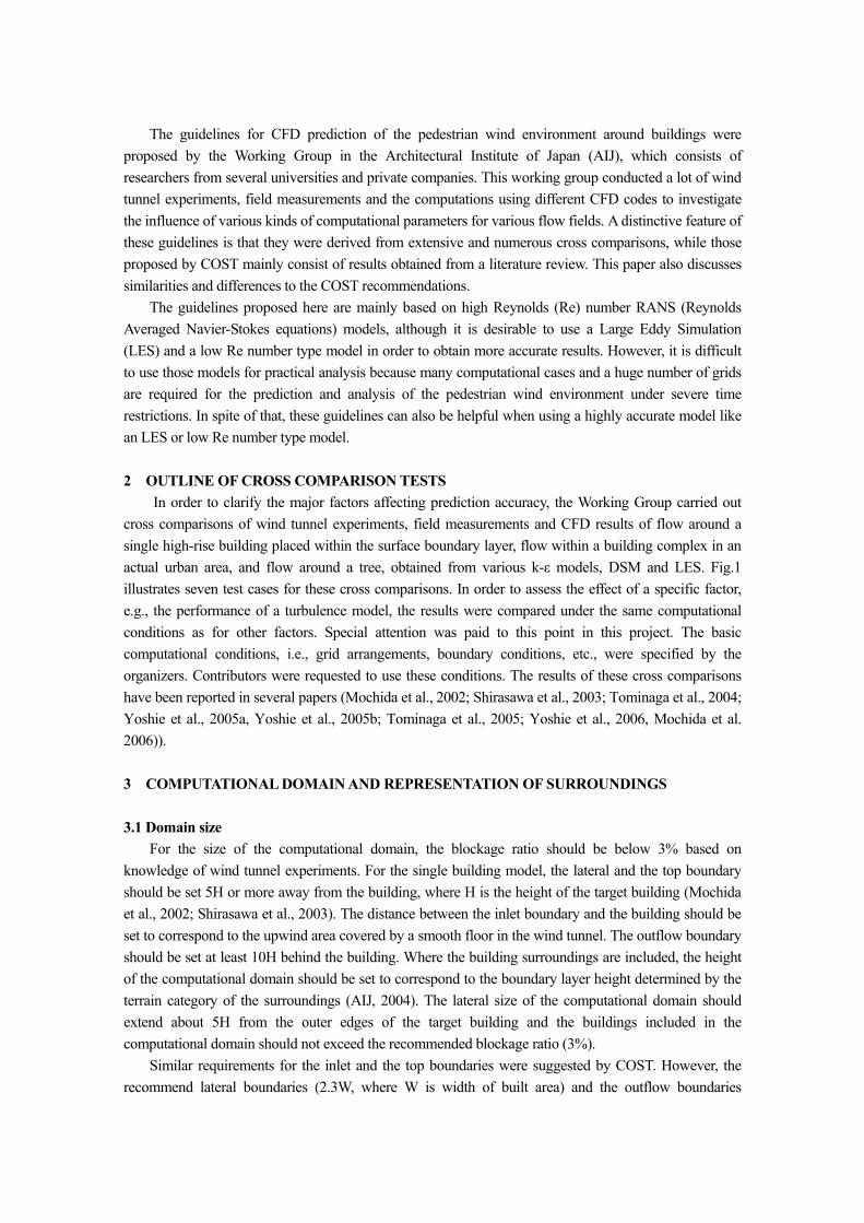
高層建物後流弱風域におけるガス拡散性状に関する LES と Durbin 型 k-εモデルの比較
Comparison of LES and Durbin type k-ε model for gas diffusion in weak wind region behind a building
白 澤 多 一*, 遠 藤 芳 信**, 義 江 龍 一 郎***
持 田 灯****, 田 中 英 之* Taichi SHIRASAWA, Yoshinobu ENDO, Ryuichiro YOSHIE
Akashi MOCHIDA, Hideyuki TANAKA
Flow and diffusion fields around a building were predicted by LES and Durbin type k-ε model. The prediction accuracy of the both models was assessed by comparing their results with those obtained by wind tunnel test. The results of LES showed good agreement with experimental data in terms of mean wind velocity, turbulence statistics and mean gas concentration, while the significant differences were observed between the results of the experiment and the Durbin type k-ε model concerning the flow and diffusion fields in the wake region behind the building. This is mainly due to the fact that the periodic motions caused by the vortex shedding were not reproduced by this model.
Keywords: Large eddy simulation, Pollutant diffusion, turbulent diffusion flux, vortex shedding, High rise building, wind tunnel experiment
ラージ・エディ・シミュレーション, 汚染質拡散性状, 乱流フラックス, 渦放出, 高層建物, 風洞実験
1.はじめに
近年、計算機性能の向上に伴い、数値流体力学(Computational Fluid
Dynamics: CFD)に基づく環境シミュレーション技術は、実際の市街地
を対象とした都市風環境の予測・評価に利用可能な段階に到達しつつ
ある。筆者らは日本建築学会の WG の活動の一環として、単体の建
物モデル、街区モデル、実在市街地等を対象とした CFD 解析のベン
チマークテストを実施し 1)、CFD による市街地風環境予測のためのガ
イドラインを作成した 2)。実務の場では依然として、計算負荷の小さ
いアンサンブル平均操作に基づく k-ε系のモデルが利用されることが
多いが、いわゆるビル風による強風域を予測する場合、標準 k-εモデ
ルにおける建物風上コーナーの乱流エネルギーk の過大評価 3)を抑制
するために改良が施されたモデル例えば 4)を用いれば、それなりの精度
の解が得られる 1)5)6)。しかし、改良を施された k-ε系のモデルであっ
ても、建物後流の弱風域、市街地内部の弱風域における風速の予測精
度は悪いことが明らかとなっている 1)5)6)。この弱風域は、市街地空間
内の熱拡散や汚染質拡散を予測する場合、問題となることが多く、こ
の領域の予測精度向上が求められている。
また近年、ヒートアイランド対策の一つとして市街地の風通しの確
保の重要性が広く認識されており、強風による環境障害にとどまらず、
弱風域における通風確保が非常に重要な命題となってきている。市街
地の通風性能や熱拡散、あるいは汚染質の拡散性状予測に CFD を適
用していくためには、多くの検証事例を積み重ねていくことが重要と
考えられる。k-ε系のモデルでは予測精度の悪い建物後流域、市街地
内部の弱風域を対象とする場合、計算負荷は大きいものの、アンサン
ブル平均操作を伴わない Large Eddy Simulation(以降、LES)を適用する
ことで予測精度の改善が期待できる。LES を用いた建物周りの汚染質
の拡散性状の予測に関する研究では、富永・村上・持田 7)が単体建物
後方から浮力のあるガスが排出された拡散場を対象に、解強制置換法
を用いた複合グリッドシステム、Dynamic Mixed SGS モデルの有効性
を示した。田村・中山 8)は上流側に煙源がある場合の、障壁周りの拡
散問題について LES を適用し、その予測精度、乱流物質輸送機構に
ついて考察している。また田村・中山・奥田 9)は実在する都市空間に
LES を適用し、複雑な都市形態の違いによる気流性状、濃度拡散性状
や瞬間的な高濃度の出現について議論している。これらの研究は、実
験や実測との比較を通し、平均濃度、濃度変動の予測精度の検証は行
っている。しかし都市・建物周辺における汚染質の輸送構造を議論す
るためには、平均量や変動量だけではなく、移流濃度フラックスや乱
流濃度フラックスまで含めた統計量も実験結果と比較し、汚染質の輸
送構造の再現性をも確認することが望ましい。しかし、数値解析の流
入境界条件としての気流性状や、数値計算の検証に必要な平均風速の
3 成分、変動成分、さらに乱流濃度フラックスを含む乱流統計量の測
定データが揃った風洞実験結果は、現時点では非常に少ない。また、
ヒートアイランド現象や汚染質の滞留が深刻となる、建物後方や都市
キャノーピー内等の弱風域では、温度変化に伴う浮力の影響が相対的
* 東京工芸大学 研究員・博士(工学) Researcher, Tokyo Polytechnic University, Dr. Eng. ** 東北大学大学院工学研究科 大学院生 Graduate student, Graduate School of Eng., Tohoku University *** 東京工芸大学工学部 教授・博士(工学) Prof., Faculty of Eng., Tokyo Polytechnic University, Dr. Eng. **** 東北大学大学院工学研究科 教授・工学博士 Prof., Graduate School of Eng., Tohoku University, Dr. Eng.

に大きくなるため、今後、非等温の LES の必要性も高まってくるも
のと予想されるが、そのような解析事例は未だ極めて少なく、乱流熱
フラックスを備えた風洞実験結果もほとんど無い。筆者らはこうした
対象に対する数値計算結果の検証用データを提供することを目的と
して、単体建物周辺の風速・温度・濃度の同時測定 10)11)12)13)を行い、
それらに関する平均量や各種乱流統計量を取得してきた。特に歩行者
レベルに対応する地表面付近の風速、温度、濃度のデータを数多く取
得している。
本報では、研究の第一段階として、まず単体建物周りの等温の流れ
場、拡散場の風洞実験 10)11)を対象に、LES と風工学の分野で現在用い
られることの多い Durbin 型の k-εモデル 4)の解析を行い、移流・乱流
フラックスによる濃度輸送構造までをも含めて実験結果と比較して、
両モデルの予測精度の評価を行った結果を報告する。なお、本報中の
主要な記号は最後にまとめて示す。
2.風洞実験概要
本解析対象は、数値計算結果の予測精度検証用データを提供するた
めに筆者らが実施した等温の境界層流中に建つ建物周辺の流れ場・濃
度場の風洞実験 10)11)と同一の対象とした。以下にその概要を示す。
東京工芸大学の境界層型風洞(測定部断面: 1.2m×1.0m)中に、図 1
に 示 す 建 物 高 さ : H が 200mm 、 建 物 幅 :W 、 奥 行 き :D が
100mm(H:W:D=2:1:1)の建物模型を設置し、その周辺の流れ場や濃度
場の測定を行った。ガス排出点は、建物模型から風下側 50mmの床面
とし、ここに排出孔(φ2mm)を設け、0.35 l/min で C2H4(エチレンガス)
を排出した。風洞気流にはべき指数約 1/4 の乱流境界層を再現し、そ
の乱れの長さスケールは実大気の 1/300 程度であった。建物高さ H と
軒高風速<uH>により求めたレイノルズ数は約 56,000 である。風速の
測定にはスプリットフィルムプローブ、濃度の測定には水素炎式高速
炭化水素計を用い、風速と濃度の同時測定を行った。サンプリング周
波数は 1,000Hzとし、120秒間に 120,000個のデータを測定している。
なお、風洞実験では、建築分野では示されることが少ない不確かさ解
析 14)を行っており、測定データの信頼性を付与している。
3.数値流体解析の概要
3.1 計算ケース
LES の SGS モデルには標準 Smagorinsky モデルを用いた。
Smagorinsky 係数は 0.1215)とし、Van Driest 型の damping function を grid
scale に乗じた。また、SGS シュミット数は 0.57)とした。
k-εモデルの解析では標準型、Durbin モデル 4)の 2 ケースを行った。
3.2 計算手法
表 1 に計算条件を示す。計算領域は、流れ方向には建物背面より風
上側に 3H、風下側に 7. 5H とした。高さと幅は実験を行った風洞の
測定断面と同一とした。LES の流入境界条件としては、片岡らの方法
16)に準じて、別途流入変動風を生成した注 1)。また床面からのガス排
出口からの排出風速は一定値とし、乱れは与えなかった注 2)。なお、
以下に示す LES の解析結果はすべて grid –scale の値である注 3)。
4.流れ場の比較
4.1 再付着距離(表 2)
屋上面及び建物後方床面の再付着距離を表 2 に示す。LES と Durbin
モデルは屋上面の逆流を再現するが、かねてから指摘 3)されているよ
うに、標準型 k-εモデルは屋上面の逆流が再現されない。建物後方床
面の再付着距離 XFはすべてのモデルで実験より長めに評価している
ものの、LES は大幅に実験に近づく。これ以降、k-ε系のモデルにつ
いては、屋上面の逆流を再現し、建物後方の循環流の過大評価が標準
型よりも小さい Durbin モデルを取り上げ比較する。
4.2 平均風速ベクトル(図 2,3)
図 2 に鉛直中心断面における平均風速ベクトルを示す。LES の結果
は後方循環流の広さが Durbin モデルに比べ実験に近い。図 3 には、
水平断面における平均風速ベクトルを示す。Durbin モデルは建物後
方の両コーナー付近に形成される 2 つの渦の中心が実験、LES に比べ、
センターラインから x2 方向にやや離れた場所に位置し、また渦の形
状が風下側に長く延びている。また建物側面で Durbin モデルは、実
験、LES に比べ大きなはく離流が生じ、再付着していない。
4.3 平均スカラー風速の水平分布(図 4)
図 4 に床面付近のスカラー風速の水平分布を示す。Durbin モデルは
実験に比べ、建物後方の弱風領域が後方に長く拡がっている。一方、
LES は弱風領域の広さや分布形状が全体的に実験に近い。このような
差は既報 6)15)で指摘したように、LES では渦放出に伴う周期的な変動
が再現されるのに対して、k-εモデルではこれが再現されていないこ
とにより生じるものと考えられる。
4.4 乱流エネルギーの鉛直・水平分布(図 5, 6, 7(1), 8(1))
図1 解析対象と座標系 表 1 計算条件
解析領域 10.5H(x1)×6.0H(x2)×5.0H(x3) x2、x3方向の解析領域の広さは風洞の断面と一致させている。
メッシュ分割 k-ε:76(x1)×45(x2)×37(x3) LES:107(x1)×99(x2)×73(x3)
流入境界 k-ε:<u1>と k は風洞実験値を補間、
εは流入面で k の生産項 Pk=εを仮定し算出した。 LES:片岡らの方法 16)に準じて、別途流入変動風を作成した。
側面・上空境界 法線方向の速度成分をゼロとする。 諸量に関して法線方向の勾配ゼロとする。
流出境界 諸量に関して法線方向の勾配ゼロとする。
地表面境界・ 建物壁面境界
k-ε:generalized log law (滑面用) LES:Werner and Wengle により提案された 2 層モデル 17) 濃度:法線方向の勾配ゼロ
移流項スキーム k-ε :全輸送方程式に QUICK を使用。 LES:2 次精度中心差分。但し、濃度の輸送方程式の計算には
3 次精度の風上差分 18)を用いた。 計算
アルゴリズム k-ε :HSMAC 法 LES:SMAC 法
表 2 再付着距離
x1
x2
x3
<uH>=4.2 m/s
H=0
.2m
0.05m Tracer gas source
x1
x2
x3
<uH>=4.2 m/s
H=0
.2m
0.05m Tracer gas source
XR/D XF/D風洞実験 0.53 1.37
LES 0.65 2.02標準k-ε - 2.80Durbin 0.71 2.76
x1
x3
wind
D XF
XR
x1
x3
wind
D XF
XRXR/D XF/D
風洞実験 0.53 1.37LES 0.65 2.02
標準k-ε - 2.80Durbin 0.71 2.76
x1
x3
wind
D XF
XR
x1
x3
wind
D XF
XR

乱流エネルギーk の鉛直断面の分布を図 5 に示す。建物後方循環流
領域内では、Durbin モデルは実験に比べ、k を全体的に小さく予測し
ている。一方、LES は循環流域の上部付近(自由せん断層付近)を中心
として実験に比べやや大きめに k を評価しているものの、分布形状は
実験に近い注 4)。
地表面付近における k の水平分布を図 6 に示す。実験、LES は建物
側面から建物後方循環流領域内にかけて k の大きな領域が拡がるの
に対して、Durbin モデルではその傾向が再現されない。
4.5 後方循環流域内のノルマルストレスの鉛直分布(図 7(2)~(4))
建物後方循環流域内のノルマルストレスの鉛直分布を図 7(2)-(4)に
示す。ここでは図中に実験の測定の不確かさ範囲 14)を併せて示す。
なお、不確かさ範囲は、測定量の 95%がこの範囲に収まると期待さ
れる領域を示している。Durbin モデルはノルマルストレスの各成分
を過小に評価し、実験の傾向を再現していない。一方、LES は建物後
1
0 0.5 1 1.5 2‐0.5‐1
1.5
X 1/H
X 3/H
0.5
0
1
0 0.5 1 1.5 2‐0.5‐1
1.5
X 1/H
X 3/H
0.5
0
1
0 0.5 1 1.5 2‐0.5‐1
1.5
X 1/H
X 3/H
0.5
0
1
0 0.5 1 1.5 2‐0.5‐1
1.5
X 1/H
X 3/H
0.5
0
1
0 0.5 1 1.5 2‐0.5‐1
1.5
X 1/H
X 3/H
0.5
0
1
0 0.5 1 1.5 2‐0.5‐1
1.5
X 1/H
X 3/H
0.5
0
1
0 0.5 1 1.5 2‐0.5‐1
1.5
X 1/H
X 3/H
0.5
0
1
0 0.5 1 1.5 2‐0.5‐1
1.5
X 1/H
X 3/H
0.5
0
(1)実験 (2)LES (3)Durbin モデル 図 2 平均風速ベクトルの鉛直分布(x2/H=0.0)
0
0 0.5 1 1.5 2‐0.5‐1
1
0.5
X 1/H
X 2/H
‐0.5
‐1
0
0 0.5 1 1.5 2‐0.5‐1
1
0.5
X 1/H
X 2/H
‐0.5
‐1
0
0 0.5 1 1.5 2‐0.5‐1
1
0.5
X 1/H
X 2/H
‐0.5
‐1
0
0 0.5 1 1.5 2‐0.5‐1
1
0.5
X 1/H
X 2/H
‐0.5
‐1
(1)実験 (2)LES (3)Durbin モデル 図 3 平均風速ベクトルの水平分布(x3/H=0.0625)
0
0 0.5 1 1.5 2‐0.5‐1
1
0.5
X 1/H
X 2/H
‐0.5
‐1
0.5
0.1
0.8
0.1
0.5
0.30.3
0.7
0.2
0
0 0.5 1 1.5 2‐0.5‐1
1
0.5
X 1/H
X 2/H
‐0.5
‐1
10.8 0.5
0.30.10.20.20.3
0.5 0.7
0.2 0
0 0.5 1 1.5 2‐0.5‐1
1
0.5
X 1/H
X 2/H
‐0.5
‐1
0.90.7
0.50.3
0.30.3
0.5
0.7
0.2 0.10.1
0.8
0
0 0.5 1 1.5 2‐0.5‐1
1
0.5
X 1/H
X 2/H
‐0.5
‐1
0.90.7
0.50.3
0.30.3
0.5
0.7
0.2 0.10.1
0.8
(1)実験 (2)LES (3)Durbin モデル 図 4 平均スカラー風速<U>/<uH>の水平分布(x3/H=0.0625)
0.09
0.07
0.12
0.03
0.03
0.03
0.030.05
0.051
0 0.5 1 1.5 2‐0.5‐1
1.5
X 1/H
X 3/H
0.5
0
0.10.12
0.12
0.05
0.07
0.02
0.05
0.07
0.03
1
0 0.5 1 1.5 2‐0.5‐1
1.5
X 1/H
X 3/H
0.5
0
0.70.11
0.02
0.04
0.04
0.04
0.03
1
0 0.5 1 1.5 2‐0.5‐1
1.5
X 1/H
X 3/H
0.5
0
(1)実験 (2)LES (3)Durbin モデル 図 5 乱流エネルギーの鉛直分布 k /<uH>2
(x2/H=0.0)
0
0 0.5 1 1.5 2‐0.5‐1
1
0.5
X 1/H
X 2/H
‐0.5
‐1
0.05
0.070.07 0.07
0.03
0.030.01
0
0 0.5 1 1.5 2‐0.5‐1
1
0.5
X 1/H
X 2/H
‐0.5
‐1
0.05
0.08 0.070.08
0.03
0.050.03 0
0 0.5 1 1.5 2‐0.5‐1
1
0.5
X 1/H
X 2/H
‐0.5
‐1
0.050.08
0.01
0.03
0.01
0.08
(1)実験 (2)LES (3)Durbin モデル 図 6 乱流エネルギーk /<uH>2
の水平分布(x3/H=0.0625)

方循環流領域内では、x2方向のノルマルストレスをやや
実験に比べ大きめに見積もっているものの、概ね測定の
不確かさ範囲に収まり、実験との対応がよい。しかし、
x3/H>1 の領域で x2、x3方向のノルマルストレスが実験
値より大きくなっており、前述したこの領域での kの過大評
価と対応している。
4.6 後方循環流域内のノルマルストレスの水平分布
(図 8(2)~(4))
建物後方循環流域内地表面付近のノルマルストレスの水平分布を
図 8(2)-(4)に示す。全体的に Durbin モデルは x1、x2方向のノルマルス
トレスを過小評価し、x3方向のノルマルストレスを過大に評価してい
る。一方、LES は各成分ともにやや大きめな値を示し、測定の不確か
さ範囲内に収まらないが、実験同様の分布形状を再現している。
4.7 シアストレス<u1’u2’>/<uH>2の水平分布(図 9)
前述のノルマルストレスの予測精度の改善は、シアストレスの生産
項を通じてシアストレスに影響を及ぼすため、ノルマルストレスとシ
アストレスの予測精度の改善は連動するものと考えられる注 5)。そこ
0.0
0.5
1.0
1.5
2.0
0.00 0.05 0.10 0.15
X3/HExp
LES
Durbin
0.0
0.5
1.0
1.5
2.0
0.00 0.05 0.10 0.15
X3/H 不確かさ範囲
0.0
0.5
1.0
1.5
2.0
0.00 0.05 0.10 0.15
X3/H
0.0
0.5
1.0
1.5
2.0
0.00 0.05 0.10 0.15
X3/H x3
x1x1=0.0
plotting line
x3
x1x1=0.0
plotting line
x1/H=0.5
(1) k/<uH>2 (2) <u1’2>/<uH>2 (3) <u2’2>/<uH>2 (4) <u3’2>/<uH>2
図 7 建物後方循環流域内の乱流エネルギーk/<uH>2とノルマルストレス<ui’2>/<uH>2
の鉛直分布(x1/H=0.5, x2/H=0)
0.0
0.5
1.0
1.5
2.0
0 0.05 0.1
X2/HExp
LES
Durbin
0.0
0.5
1.0
1.5
2.0
0 0.05 0.1
X2/H 不確かさ範囲不確かさ範囲
0.0
0.5
1.0
1.5
2.0
0 0.05 0.1
X2/H
0.0
0.5
1.0
1.5
2.0
0 0.05 0.1
X2/Hx2
x1
plotting line
x1/H=0.5
x1=0.0
(1) k/<uH>2 (2) <u1’2>/<uH>2 (3) <u2’2>/<uH>2 (4) <u3’2>/<uH>2 図 8 乱流エネルギー k/<uH>2
とノルマルストレス<ui’2>/<uH>2の水平分布(x1/H=0.5, x3/H=0.0625)
2.55
1080
1
0 0.5 1 1.5 2‐0.5‐1
1.5
X 1/H
X 3/H
0.5
0
160
320
2040
1
0 0.5 1 1.5 2‐0.5‐1
1.5
X 1/H
X 3/H
0.5
0
2.55
1020
4080320
160
1
0 0.5 1 1.5 2‐0.5‐1
1.5
X 1/H
X 3/H
0.5
0
2.5510
2040
80
80160
320
1
0 0.5 1 1.5 2‐0.5‐1
1.5
X 1/H
X 3/H
0.5
0
2.5510
2040
80
80160
320
(1)実験 (2)LES (3)Durbin モデル 図 10 平均濃度<c>/<c0>の鉛直分布(x2/H=0.0)
0
0 0.5 1 1.5 2‐0.5‐1
1
0.5
X 1/H
X 2/H
‐0.5
‐1
2.55
10204080
160 320
0
0 0.5 1 1.5 2‐0.5‐1
1
0.5
X 1/H
X 2/H
‐0.5
‐1
2.5
5
102040
80 0
0 0.5 1 1.5 2‐0.5‐1
1
0.5
X 1/H
X 2/H
‐0.5
‐1
2.55
102040
80
160 320
(1)実験 (2)LES (3)Durbin モデル 図 11 平均濃度<c>/<c0>の水平分布(x3/H=0.0625)
(1) LES (2) Durbin モデル
図 9 シアストレス<u1’u2’>/<uH>2の水平分布(x3/H=0.0625)
0
0 0.5 1 1.5 2‐0.5‐1
1
0.5
X 1/H
X 2/H
‐0.5
‐1
-0.02
-0.010
0
0.02
0.01
00
0-0.01
0
0 0.5 1 1.5 2‐0.5‐1
1
0.5
X 1/H
X 2/H
‐0.5
‐1
-0.02 -0.01
0.02 0.01
00
0
-0.02
0
0.02

で、図 9 に LES と Durbin モデルの<u1’u2’>の水平分布を示し、比較す
る。渦放出の再現の有無の影響はシアストレス<u1’u2’>の分布に大き
く現れている。LES では建物側面から建物後方循環流域内にかけて絶
対値 0.02 で示される領域が拡がっているが、Durbin モデルではその
領域が非常に狭くなっている。この結果、Durbin モデルは x2方向の
運動量拡散が不十分となり、後方再付着距離、弱風領域の大きさが正
しく評価されなかったものと考えられる。
5.拡散場の比較
5.1 平均濃度<c>/<c0>
(1)鉛直分布(図 10)
図 10 に平均濃度の鉛直分布を示す。Durbin モデルの結果は建物背
面の高濃度の領域が建物高さ付近まで拡がり、分布形状が実験と異な
る。LES の結果は、全般に濃度がやや低くなる傾向にあるものの、
Durbin モデルに比べ、大幅に分布形状が実験に近づく。
(2)水平分布(図 11)
地表面付近の平均濃度の水平分布を図 11 に示す。LES は実験に比
べ、水平方向にガスが拡がった分布を示すものの、排出口(x1/H=0.25、
x2/H=0)と建物背面の間を中心に高濃度の領域が拡がる実験の分布形
状に近い。一方、Durbin モデルは前述のように建物からの渦放出に
伴う周期的変動が再現されない結果、x2方向の拡散が抑えられたまま
ガスは逆流に乗って地表面に沿って建物背面まで輸送される。そして、
それが前述した(図 3(3))建物側面の大きな逆流により建物側面まで拡
がっており、異なる分布の傾向を示している。
5.2 移流フラックス
(1)<u1><c>/<uH><c0>の鉛直分布(図 12)
LES は概ね実験と同様の分布性状を示しているものの、Durbin モデ
ルは建物背面の負の領域が実験に比べ広い。これは建物後方循環流が
大きめに評価されたためと考えられ、建物後方の弱風領域の大きさを
正しく評価できなかった結果と対応している。
(2) <u1><c>/<uH><c0>の水平分布(図 13)
実験結果は建物背後の弱風領域で負値を示し、建物後方コーナー付
0.5
-0.5
0
0.30.1
0.1 0.3
1
0 0.5 1 1.5 2‐0.5‐1
1.5
X 1/H
X 3/H
0.5
0
0.5-0.5
0 0.3
00.1
0.51
0 0.5 1 1.5 2‐0.5‐1
1.5
X 1/H
X 3/H
0.5
0
0.5-0.5 0 0.3
0.10.5
0.30
0
1
0 0.5 1 1.5 2‐0.5‐1
1.5
X 1/H
X 3/H
0.5
0
(1)実験 (2)LES (3)Durbin モデル 図 12 移流フラックス<u1><c>/<uH><c0>の鉛直分布(x2/H=0.0)
0
0 0.5 1 1.5 2‐0.5‐1
1
0.5
X 1/H
X 2/H
‐0.5
‐1
5 3
1
-5 10-1
0
0 0.5 1 1.5 2‐0.5‐1
1
0.5
X 1/H
X 2/H
‐0.5
‐1
5 3
1
-5 0-1-31
0
0
0 0.5 1 1.5 2‐0.5‐1
1
0.5
X 1/H
X 2/H
‐0.5
‐1
5 31
-5 0-1
1-5
(1)実験 (2)LES (3)Durbin モデル
図 13 移流フラックス<u1><c>/<uH><c0>の水平分布(x3/H=0.0625)
0
0 0.5 1 1.5 2‐0.5‐1
1
0.5
X 1/H
X 2/H
‐0.5
‐1
0
-13
3 1
0
-3
-3
0
0 0.5 1 1.5 2‐0.5‐1
1
0.5
X 1/H
X 2/H
‐0.5
‐1
0
-105
-50
1
0
0
0 0.5 1 1.5 2‐0.5‐1
1
0.5
X 1/H
X 2/H
‐0.5
‐1
0
05
-50
0
5
-5
-5
5
(1)実験 (2)LES (3)Durbin モデル 図 14 移流フラックス<u2><c>/<uH><c0>の水平分布(x3/H=0.0625)
0.5
0
00.10.3
0.1
0.10.31
0 0.5 1 1.5 2‐0.5‐1
1.5
X 1/H
X 3/H
0.5
0
0.5 00
0.3 0.1
-0.1
-0.5
1
0 0.5 1 1.5 2‐0.5‐1
1.5
X 1/H
X 3/H
0.5
0
0.5
-0.10.1
-0.3-0.5
0
0
0
1
0 0.5 1 1.5 2‐0.5‐1
1.5
X 1/H
X 3/H
0.5
0
(1)実験 (2)LES (3)Durbin モデル 図 15 移流フラックス<u3><c>/<uH><c0>の鉛直分布(x2/H=0.0)

近から風下側には正値の領域が拡がっている。LES は実験と同様の分
布性状を示すものの、実験に比べ、建物後方コーナー付近から風下側
に正値を示す領域が広い。一方、Durbin モデルは実験と異なり、建
物背後から側面まで負値を示す領域が拡がっている。先に示したよう
に(図 3(3))、Durbin モデルは建物側面の逆流が大きく、建物背面の
wake と一体化している。その結果、この逆流によって建物背面の高
濃度ガスが建物側面まで移流されており、建物側面まで高濃度の領域
が拡がった分布を示した平均濃度分布(図 11(3))と対応している。ま
た建物側面まで輸送されたガスが建物風上コーナーからの剥離流に
より移流される結果、正値を示す領域が実験より風上側まで拡がって
おり、実験、LES と大きく異なる分布性状を示す。
(3) <u2><c>/<uH><c0>の水平分布(図 14)
LES は実験に比べ、移流フラックス<u2><c>/<uH><c0>の絶対値が大
きく、その領域も広いものの、実験と同様の分布性状を示す。実験と
LES は排出口(x1/H=0.25)後方で中心軸を挟み、正値および負値を示す
領域が明確に現れるのに対し、Durbin モデルには見られない。
(4) <u3><c>/<uH><c0>の鉛直分布(図 15) LES は実験とほぼ同様の分布を示すが、建物背面付近の正値を示す
領域が実験に比べてやや狭い。これは、建物背面高濃度領域の鉛直方
向への広がりが実験に比べて、やや小さくなった結果(図 10(2))と対
応している。一方、Durbin モデルは建物背面で正値を示すものの、
上方に行くに従い正値を示す領域が減少する傾向が再現されない。こ
れは建物背面の高濃度の領域が建物高さ付近まで拡がる結果(図
10(3))と対応している。
5.3 乱流拡散フラックス
(1)<u1’c’>/<uH><c0>の鉛直分布(図 16)
LES は建物背面付近の乱流拡散フラックス<u1’c’>の大きな領域が
実験に比べやや狭いものの、実験に近い。一方、Durbin モデルは排
出口から風下側への<u1’c’>の広がりが見られない。これは排出口よ
り風下側は低濃度であり、濃度勾配も小さく(図 10(3))、勾配拡散近
似より求まる<u1’c’>は非常に小さな値を示したためである。
(2)<u1’c’>/<uH><c0>の水平分布(図 17)
1
0 0.5 1 1.5 2‐0.5‐1
1.5
X 1/H
X 3/H
0.5
0
0.50.3
0
-0.1
-0.1
‐0.5
1
0 0.5 1 1.5 2‐0.5‐1
1.5
X 1/H
X 3/H
0.5
0
0.50.3
0
-0.1
‐0.5
1
0 0.5 1 1.5 2‐0.5‐1
1.5
X 1/H
X 3/H
0.5
0
0.50.3
00.1
‐0.5
(1)実験 (2)LES (3)Durbin モデル 図 16 乱流拡散フラックス<u1’c’>/<uH><c0>の鉛直分布 (x2/H=0)
0
0 0.5 1 1.5 2‐0.5‐1
1
0.5
X 1/H
X 2/H
‐0.5
‐1
50
1
-1‐1
-1
0
0 0.5 1 1.5 2‐0.5‐1
1
0.5
X 1/H
X 2/H
‐0.5
‐1
5
01
-1
3
0 0
-3‐5
0
0 0.5 1 1.5 2‐0.5‐1
1
0.5
X 1/H
X 2/H
‐0.5
‐1
5
0
1
3 5
(1)実験 (2)LES (3)Durbin モデル
図 17 乱流拡散フラックス<u1’c’>/<uH><c0>の水平分布(x3/H=0.0625)
0
0 0.5 1 1.5 2‐0.5‐1
1
0.5
X 1/H
X 2/H
‐0.5
‐1
50
1 3
-1-3-5
0
0 0.5 1 1.5 2‐0.5‐1
1
0.5
X 1/H
X 2/H
‐0.5
‐1
50
1
-1
3
-3-5
0
0 0.5 1 1.5 2‐0.5‐1
1
0.5
X 1/H
X 2/H
‐0.5
‐1
5 0
1
-1
-5
1
-1
0
(1)実験 (2)LES (3)Durbin モデル 図 18 乱流拡散フラックス<u2’c’>/<uH><c0>の水平分布(x3/H=0.0625)
0.5
00.1
0.3
01
0 0.5 1 1.5 2‐0.5‐1
1.5
X 1/H
X 3/H
0.5
0
0.5
0
0.1
0.3
0.1
0
1
0 0.5 1 1.5 2‐0.5‐1
1.5
X 1/H
X 3/H
0.5
00.5 0
0.3
0
0.1
0.3 0.11
0 0.5 1 1.5 2‐0.5‐1
1.5
X 1/H
X 3/H
0.5
0
(1)実験 (2)LES (3)Durbin モデル 図 19 乱流拡散フラックス<u3’c’>/<uH><c0>の鉛直分布(x2/H=0.0)

実験では、建物後方コーナー付近で負値を示し、ガス排出口付近
(x1/H=0.25)で正の領域が拡がっている。LES はどちらの領域もやや広
めであるが、この傾向を再現している。しかし、Durbin モデルは建
物後方コーナー付近で負値を示さず、またガス排出口付近の正の領域
の x2方向への広がりが小さい。
(3)<u2’c’>/<uH><c0>の水平分布(図 18)
勾配拡散近似で算出される Durbin モデルの拡散フラックスは LES
に比べ、水平方向への拡がりが小さい。これは、Durbin モデルは建
物からの渦放出が再現されない結果、x2方向の拡散が抑えられたこと
によるものである。一方、LES には渦放出に伴う周期的変動が含まれ
ており、その結果、建物後方循環流域の広範囲で x2 方向の濃度輸送
が行われている。その結果、実験と同様に水平方向に広がりを持った
平均濃度分布(図 11(2))になったものと考えられる。
LES の結果は、前述のように、建物後方循環流内のノルマルストレ
ス(図 7(3),図 8(3))、拡散フラックス<u2’c’>/<uH><c0>を実験に比べ、や
や過大評価しており、今回の LES の結果は渦放出に伴う x2方向の拡
散がやや過大となっており、そのため、LES では実験に比べ、水平方
向に拡がった平均濃度分布(図 11(2))になったと考えられる。この点
については、乱流シュミット数の与え方、SGS モデルを含め、検討
の余地がある。
(4)<u3’c’>/<uH><c0>の鉛直分布(図 19)
LES の結果は、実験に比べ<u3’c’>の大きな領域が鉛直方向に狭く、
風下方向に拡がる傾向があるが、実験と同様の傾向を示す。一方、
Durbin モデルの結果は排出口から建物背面にかけて<u3’c’>が正値を
とる点では実験と同様の傾向だが、排出口から風下側への広がりがな
く、実験と異なる。これは、排出口の風下側の負値をとる領域で
は∂<c>/∂x3>0 の濃度勾配が生じており(図 10(3))、勾配拡散近似
により算出された<u3’c’>が負となるため、実験、LES と異なる分布を
示していることによる。
5.4 |<uα’c’>|/(|<uα><c>|+|<uα’c’>|)の鉛直・水平分布(図 20,21,22)
トータルのフラックスに占める乱流拡散フラックスの寄与を調べ
るため、実験結果、LES、Durbin モデルより算出した移流フラックス
の絶対値と乱流拡散フラックスの絶対値の和に対する乱流拡散フラ
ックスの絶対値の比である|<uα’c’>|/(|<uα><c>|+|<uα’c’>|)の x1、x2 成
分の水平分布を図 20,図 21 に示す。x1成分では、実験、LES ともに建
物側面と建物後流域で大きな値を示し、乱流拡散フラックス<u1’c’>
の影響が強い。一方、Durbin モデルはその傾向を再現しない。x2成分
は、実験結果は建物側方から建物後方弱風域にかけて、移流フラック
スに対し乱流拡散フラックス<u2’c’>の寄与が大きい領域が拡がって
いる。LES は Durbin モデルよりも建物弱風域の乱流拡散フラックス
の影響が強い領域が広く、実験に近づく。前述のように建物後方から
の渦放出に伴う周期的変動が再現されたことにより、この領域での
LES の乱流拡散フラックス<u2’c’>の予測精度が向上したことが、建物
背面付近における濃度分布が実験に近づいた要因と考えられる。
x3成分の鉛直分布を図 22 に示す。LES は、実験の傾向を概ね再現
する。一方、Durbin モデルは、後方循環流域内で移流フラックスが
卓越している領域が広く、実験、LES と異なる傾向を示す。
6.結論
境界層流中に置かれた建物周りの流れ場・濃度場の解析を行い、建
物後方の弱風域に着目して、風洞実験との比較を通し、LES、k-ε系
モデルの予測精度の比較を行った。
(1) LES は、渦放出に伴う周期的変動が再現されることにより、k-ε系
モデルに比べ建物後方の循環流領域の大きさ、地表面付近の弱風領域
の平均風速分布、ノルマルストレスの予測精度が大幅に改善され、そ
の有効性が確認された。
(2) 渦放出に伴う周期的変動は流れ場だけではなく拡散場にも大きな
影響を及ぼす。LES は k-εモデルに比べ、流れ場の予測精度が改善さ
れることにより、移流フラックスの予測精度が向上する。また勾配拡
散近似に基づく k-ε系モデルは乱流拡散フラックスが実験の傾向を捉
えきれないのに対し、LES はその分布性状が実験の傾向と定性的に一
致する。これらの結果より k-ε系モデルに比べ、LES は実験と対応す
る平均濃度分布の形状が得られたものと考えられる。
(3)しかし、今回の LES は渦放出に伴う x2方向の物質輸送をやや過大
に評価した。乱流シュミット数の与え方、SGS モデルについて検討
の余地がある。
[記号] xi :空間座標の 3 成分(i=1:主流方向、i=2:スパン方向、i=3:鉛直方向) ui :風速ベクトルの i 成分
00 0.5 1 1.5 2‐0.5‐1
0.5
X 1/H
X 2/H0.6 0.1
0.10.3
0.30.5
0.6
0
0 0.5 1 1.5 2‐0.5‐1
0.5
X 1/H
X 2/H
0.1
0.10.3
0.2
0.9
0.30.40.60.9
0.50.40.1 00 0.5 1 1.5 2‐0.5‐1
0.5
X 1/H
X 2/H0.1
0.40.90.1
0.1 0.7
0.9
0.50.7
0.7
(1)実験 (2)LES (3)Durbin モデル 図 20 |<u1’c’>|/(|<u1><c>|+|<u1’c’>|)の水平分布(x3/H=0.0625)
00 0.5 1 1.5 2‐0.5‐1
0.5
X 1/H
X 2/H
0.1 0.9
0.90.3
0
0 0.5 1 1.5 2‐0.5‐1
0.5
X 1/H
X 2/H0.1
0.9
0.30.50.60.70.4
0.8
0.9
0.40.9
0.7 00 0.5 1 1.5 2‐0.5‐1
0.5
X 1/H
X 2/H 0.10.3
0.90.1
0.2 0.30.7
0.9
0.10.2
(1)実験 (2)LES (3)Durbin モデル 図 21 |<u2’c’>|/(|<u2><c>|+|<u2’c’>|)の水平分布(x3/H=0.0625)
1
0 0.5 1 1.5 2‐0.5‐1 X 1/H
X 3/H
0.5
0
0.70.6 0.5
0.3
0.10.3
0.70.5 0.9
1
0 0.5 1 1.5 2‐0.5‐1 X 1/H
X 3/H
0.5
0
0.90.5
0.3
0.10.3 0.7
0.5
0.7 0.6
1
0 0.5 1 1.5 2‐0.5‐1 X 1/H
X 3/H
0.5
0
0.3
0.1
0.90.9
0.1
0.2
0.4
0.10.3
(1)実験 (2)LES (3)Durbin モデル 図 22 |<u3’c’>|/(|<u3><c>|+|<u3’c’>|)の鉛直分布(x2/H=0.0)

f :変数 f の瞬時値 <f> :変数 f の時間平均値 f’ :時間平均からのずれ(=f-<f>) H :建物高さ(0.2m) <uH> :流入境界における高さ H の平均風速(u1成分) (4.2m/s) q :ガス発生量 <C0> :規準濃度(q/<uH>H2) <U> :平均スカラー風速(<U>=(<u1>2+<u2>2+<u3>2)0.5)
謝辞
本研究は、平成 19 年度科学研究費補助金基盤研究(B)、課題番号 19360265:
「「鉛直方向の風の道」による臨海過密都市のヒートアイランド・大気汚染対
策の提案」、及び東京工芸大学 21 世紀 COE プログラムからの助成を受けてい
る。また本計算は、日本建築学会屋外環境予測・評価小委員会(主査:持田)
「市街地の通風・拡散予測 WG(主査:義江)」の活動の一環として行われた。
WG 委員の方々には貴重な御助言・ご協力を頂きました。また本稿作成にあた
り、東京工芸大学大学院生小林剛氏の協力を得ました。ここに記して謝意を表
します。
注
注 1) 流入変動風は片岡らの方法 16)に準じて作成した。流入変動風生成のため
の計算領域は、5H(x1)×6H(x2)×5H(x3)、計算格子数は 144,540 である。SGS
モデルは本計算と同じ標準 Smagorisky モデルを用いた。モデル係数は既往
の研究 19)を参考にして Cs=0.1 を使用した。この計算により、無次元時間(t・
<UH>/H)で 105 の間の変動成分を取得し、この結果を周期条件として、本計
算の流入変動風として用いた。図 23 に平均風速と乱流エネルギーの鉛直分
布を風洞実験とあわせて示す。
0.0
1.0
2.0
3.0
4.0
5.0
0 0.5 1 1.5
<u>/<uH>
X3/H
Exp LES
0.0
1.0
2.0
3.0
4.0
5.0
0 0.025 0.05
<k>/<UH>2
不確かさ範囲不確かさ範囲
図 23 流入変動風の性状
注 2) エチレンガスの排出口での Re を概算する。管内流のレイノルズ数は、
Re=<w>d/ν
ここで、エチレンガスの 300[K]の動粘性係数νは 8.99×10⁻⁶ [m2/s] 20)である。
エチレンガスは排出孔(d=2[mm])より 0.35 l/min(q=5.83×10-6 [m3/s])で排出し
ており、管断面の平均流速<w>は 1.86[m/s]となる。したがって、
Re=1.86×2×10-3/(8.99×10-6)=414
となり、本実験の場合は層流であると考えられる。
注 3) LES は、無次元時間差分間隔(t・<UH>/H)=4.2×10-4で解析し、無次元時間
(t・<UH>/H)で 210 の間のデータを平均化して諸量を算出した。また k-ε系の
モデルは、HSMAC法に基づく非定常解析(無次元時間差分間隔(t・<UH>/H)=1.05×10-3)
を行ったが、渦放出に伴う周期的変動は再現されなかった。
注 4) 既往の研究 3)でも、標準 Smagorinskyモデルを用いた立方体周りの流れの
解析において、自由せん断層付近の k の過大評価は報告されており、本計算
も同様の傾向である。
注 5) シアストレス-<u1’u2’>の輸送方程式の生産項 P12は、次式で表される。
kk
kk x
uuu
xu
uuP∂
∂′′−
∂
∂′′−= 1
22
112
3
132
3
231
2
2
1
121
2
122
1
211 x
uuu
xu
uuxu
xu
uuxu
uuxu
uu∂
∂′′−
∂∂
′′−⎟⎟⎠
⎞⎜⎜⎝
⎛
∂∂
+∂
∂′′−⎟
⎟⎠
⎞⎜⎜⎝
⎛
∂∂
′′+∂
∂′′−=
参考文献
1) 日本建築学会:流体数値解析による市街地風環境の予測・評価ガイドブッ
ク-ガイドラインと検証データ-,2007
2) A. Mochida, Y. Tominaga, R. Yoshie:AIJ Guideline for Practical Applications of
CFD to Wind Environment around Buildings, The 4th International Symposium on
Computational Wind Engineering (CWE2006), Yokohama, 533-536, 2006
3) 持田灯,村上周三,林吉彦:立方体モデル周辺の非等方乱流場に関する k-εモ
デルと LES の比較 -乱流エネルギー生産の構造とノルマルストレスの非等
方性の再現に関して-,日本建築学会計画系論文集 423, 23-31, 1991.5
4) P.A. Durbin, Technical Note: On the k-ε stagnation point anomaly, Int. J. Heat and
Fluid Flow, 17 ,9-90, 1996
5) Y. Tominaga, A. Mochida, T.Shirasawa, R. Yoshie, H. Kataoka, K. Harimoto and T.
Nozu: Cross Comparisons of CFD Results of Wind Environment at Pedestrian
Level around a High-rise Building and within a Building Complex, Journal of Asian
Architecture and Building Engineering, vol.3 no.1 ,63-70, 2004
6) 富永禎秀,持田灯,村上周三,佐脇哲史:高層建物周辺気流の CFD 解析におけ
る各種改良 k-εモデルの比較,日本建築学会計画系論文集,556,47-54, 2002.6
7) 富永禎秀,村上周三,持田灯:複合グリッドを用いた Dynamic Mixed SGS モデ
ル による建物周辺のガス拡散の LES, 日本建築学会計画系論文
集,496,53-58,1997.6
8) 田村哲郎,中山浩成:障壁まわりの乱流場・拡散場の LES 解析、日本風工学
会論文集,第 30 巻,第 2 号,21-36,2005
9) 田村哲郎,中山浩成,奥田泰雄:実在都市における空間発達型境界層乱流中の
大気拡散に関する LES 解析,日本建築学会環境系論文集,604,31-38,2006.6
10) 田中英之,義江龍一郎,白澤多一:単独建物周りの流れ場と拡散場の計測とそ
の不確かさ評価 その 1 スプリットフィルムプローブの精度確認と適切な
風速測定方法,日本建築学会大会学術講演梗概集(D2), 819-820 , 2006
11) 白澤多一,義江龍一郎,田中英之:単独建物周りの流れ場と拡散場の計測とそ
の不確かさ評価 その 2 不確かさの範囲を併記した風洞実験結果,日本建
築学会大会学術講演梗概集(D2), 821-822, 2006
12) 小林剛,義江龍一郎,田中英之,白澤多一:弱風域を対象とした流れ場・温度
場・拡散場に関する風洞実験と数値解析 (その 1) 非等温流れ場の風速・
温度・濃度の同時測定手法と平均量の測定結果,日本建築学会大会学術講
演梗概集(D2), 695-696, 2007
13) 田中英之,義江龍一郎,小林剛,白澤多一:弱風域を対象とした流れ場・温度
場・拡散場に関する風洞実験と数値解析 (その 2) 非等温流れ場における
熱フラックス,濃度フラックス等の乱流統計量,日本建築学会大会学術講
演梗概集(D2), 697-698, 2007
14) 日本規格協会:計測における不確かさの表現ガイド,1996
15) 富永禎秀,持田灯,村上周三,佐脇哲史:建物後方の周期的変動と再付着距離
の予測精度に関する検討 LES による高層建物周辺気流の解析, 日本建築学
会環境系論文集,581,45-51, 2004.7
16) 片岡浩人,水野稔:流入変動風を用いた三次元角柱周りの気流解析,日本建築
学会計画系論文集,523, 71-77, 1999.9
17) H. Werner and H. Wengle: Large-eddy simulation of turbulent flow over and around
a cube in plate channel:Proc.8th Symp. on Turbulent shear Flows, 19-4,
155-158,1991
18) 大宮司久明,三宅裕,吉澤徴編:乱流の数値流体力学, 東京大学出版会
19) 石田義洋,持田灯,富永禎秀,白澤多一:流入変動風を同時生成した建物周辺
気流の LES,第 17 回数値流体シンポジウム,E6-1,2003
20) 日本機械学会:伝熱工学資料(改訂第 4 判),1986

1,3) Researcher 2,5) Professor 4,6) Graduate Student
Cross Comparison of CFD Results of Gas Diffusion in Weak Wind Region behind a High-rise Building
*Taichi Shirasawa1) Ryuichiro Yoshie2) Hideyuki Tanaka3) Tsuyoshi Kobayashi4)
Akashi Mochida5) Yoshinobu Endo6)
1)2)3)4) Graduate School of Eng., Tokyo Polytechnic University, Iiyama 1583, Atsugi, Japan,
5)6) Graduate School of Eng., Tohoku University, Aoba-ku 6-6-11-1202, Sendai, Japan, 1)[email protected]
ABSTRACT
Flow and diffusion fields around a building have been predicted by various RANS models (Standard k-ε model, RNG k-ε model, realizable k-ε model, Reynolds stress model) and LES. The prediction accuracy was assessed by comparing the results with those obtained by wind tunnel tests. The LES results showed good agreement with the experimental data in terms of mean wind velocity, turbulence statistics and mean gas concentration, while significant differences were observed between the results of the experiment and the RANS model concerning the flow and diffusion fields in the wake region behind the building. This is mainly because the periodic motions caused by the vortex shedding were not reproduced by the RANS models. INTRODUCTION
Recently, numerical prediction of wind and the thermal environment in an actual urban area has been carried out in the practical design stage using Computational Fluid Dynamics (CFD). In order to formulate guidelines for proper use of CFD for calculation of the wind environment, a working group was organized by the Architectural Institute of Japan (Mochida et al., 2006). The present authors conducted cross comparisons among CFD results for flow around a single building model, a high-rise building located in a city and building complexes in actual urban areas (Architectural Institute of Japan, 2007). For practical use, the k-ε model is still favorable due to its computational cost effectiveness. However, it is well known that the standard k-ε model has the serious drawback that it overestimates turbulent energy, k, in the

impinging flow region (Murakami et al., 1990). Several revised k-ε models have been proposed to overcome this drawback. Revised k-ε models (e.g. Durbin, 1996) provide adequate predictions for strong wind near the separation region close to the ground surface (Architectural Institute of Japan, 2007, Tominaga et al, 2004, Tominaga et al., 2008). However, it is known that the prediction results given by these modified k-ε models are poor in the wake region behind a building and in street canyons in urban areas (Architectural institute of Japan, 2007, Tominaga et al., 2004, Tominaga et al., 2008). When predicting thermal or pollutant diffusion in urban areas, it is essential to accurately predict turbulent flows in these locations. In addition, the importance of air ventilation in urban areas is now broadly recognized as a countermeasure to the urban heat island phenomenon, so it is becoming extremely important to ensure air ventilation in weak wind regions. In order to apply CFD to the estimation of air ventilation, thermal diffusion, and pollutant diffusion in urban areas, it is crucial to assess the performance of turbulence models for these problems. Thus, to generate data to validate numerical calculation results, the present authors carried out simultaneous measurements of wind velocity and gas concentration around a building (Tanaka et al., 2006) and obtained their time-averaged values and turbulence statistics. In particular, we obtained a large amount of data on wind velocity and gas concentration near the ground surface, which corresponds to pedestrian level, in this wind tunnel experiment.
The purpose of this work was to examine the accuracy of CFD predictions of heat and pollutant diffusion around buildings and in street canyons in non-isothermal flow. As the first step of this work, we carried out cross comparisons of CFD results of a gas diffusion field around a high rise building in isothermal flow by various RANS models (i.e., the standard k-ε model, several revised k-ε models and the Reynolds Stress Model) and Large eddy simulation. The prediction accuracy of these models and the computational method is discussed by comparing their results with those of the wind tunnel experiment. The symbols used in this paper are defined on the last page. OUTLINE OF NUMERICAL ANALYSIS Flowfield analyzed for this study
The flow and concentration fields around a building within the isothermal boundary layer were selected for this study. Detailed measurements were reported by the present authors (Tanaka et al. 2006), as outlined below. The experiment was conducted in the wind tunnel (cross section at measurement part: 1.2 m × 1.0 m) of Tokyo Polytechnic University. The model building had a height (H) of 200 mm, a width (W) of 100 mm, and a depth (D) of 100 mm (H:W:D = 2:1:1) as shown in Figure 1, and was located in a turbulent boundary layer with a power index of about 1/4. A point gas source was set on the floor 50 mm leeward of the model building. Tracer gas (C2H4: ethylene) was released from a hole (diameter: 2 mm) at a flow rate of 0.35 ℓ/min. The Reynolds number based on H (building height) and <uH> (inflow velocity at building height) was about 56,000. The wind velocity and the gas concentration were measured simultaneously using a split film probe and a fast response flame ionization detector. The sampling frequency was set at 1,000 Hz, to obtain 120,000 data in 120 seconds. In this experiment, the present authors conducted uncertainty analysis (Kirkup and Frenkel, 2006) to check the reliability of the measurement data.

Fig.1 Flowfield analyzed for this study Outlines of computations of RANS and LES
For turbulence modeling, we examined the standard k-ε model, the revised k-ε models (the RNG (Yakhot et. al, 1992) and realizable (Shih et. al, 1995) models), and the Reynolds stress model (RSM) (Gibson and Launder, 1978). The commercial code FLUENT was used for the calculation with the RANS model. A self-developed code was used for the analysis of the LES. Table 1 shows calculation conditions for the k-ε models and RSM. In the RSM, Reynolds stress <ui'uj'> was determined by solving the transport equation of <ui'uj'>, but turbulent diffusion flux <ui'c'> was calculated using the gradient-diffusion approximation (eddy viscosity modeling), instead of solving the transport equation of turbulent diffusion flux <ui'c'>. Table 2 shows calculation conditions for the LES. The standard Smagorinsky-type sub-grid model was applied in the LES computation. The Smagorinsky constant was set to 0.12 (Tominaga et .al, 2008), and the Van Driest-type damping function was used to account for the near wall effect. In addition, the SGS Schmidt number was set to 0.5 (Tominaga et al., 1997). For the inflow boundary condition of the LES, the velocity fluctuations were generated using the method proposed by Kataoka and Mizuno (Kataoka and Mizuno, 2002). The velocity of the gas discharged from the hole in the floor was set constant, and no turbulence was added. The following computational results of the LES are grid-scale values.
Unsteady-State calculations were performed for all the models but periodic fluctuations due to the vortex shedding were not reproduced except in the LES.
x1
x2
x3
UH=4.2 m/s
H=0
.2m
0.05m Tracer gas source
x1
x2
x3
UH=4.2 m/s
H=0
.2m
0.05m Tracer gas source

Table 1 Calculation conditions for RANS
Computational domain The computational domain covers 12.5H in the streamwise (x1), 6.0H in the lateral (x2) directions and 5.0H in the vertical (x3) direction.
Grid discretization 109(x1)×66(x2)×45(x3)
Inflow boundary
The interpolated values of <u> from the experimental results were imposed. The value of ε was obtained from the relation Pk=ε. The interpolated values of k from the experimental results were imposed for thek-ε models.
The interpolated values of <ui'uj'> from the experimental results were imposed for the RSM
Downstream boundary Zero gradient condition was used.
Lateral, upper, Ground and Building surfaces of
the computational domain
The generalized log law for a smooth wall was adopted. In the RSM, Reynolds stress at wall-adjacent cells are given by: <uτ'uτ'>/k=1.098, <uη'uη'>/k=0.247, <uλ'uλ'>/k=0.655, -<uτ'uη'>/k=0.255 (τ: tangential coordinate, η: normal coordinate, λ: binormal coodinate) Symmetry boundary conditions (slip walls) were used for the transport equation of k in the k-ε models and the RSM.
Scheme for Convection terms The QUICK scheme was applied to all convection terms.
Table 2 Calculation conditions for LES
Computational domain The computational domain covers 10.5H in the streamwise (x1), 6.0H in the lateral (x2) directions and 5.0H in the vertical (x3) direction.
Grid discretization 107(x1)×99(x2)×73(x3)
Inflow boundary The velocity fluctuations were generated using an artificial generation method proposed by Kataoka & Mizuno (Kataoka and Mizuno, 2002)
Downstream boundary Zero gradient condition was used. Lateral and upper
surfaces of computational domain
The normal gradients of tangential velocity components and the normal velocity components were set to zero at the upper and side faces of the computational domain.
Ground surface and Building surface
boundary
Werner and Wengle’s approach (Werner and Wengel, 1991) was adopted, in which a linear or a 1/7 power law distribution of the instantaneous velocity was assumed.
Scheme for Convection terms
A second-order centered difference scheme was adopted for the spatial derivative, except for the convection terms in the transport
equations of the gas concentration. For the convection terms of
the transport equation of the gas, a third-order upwind difference
scheme (Leonard, 1981) was used.

RESULTS AND DISCUSSIONS Reattachment lengths
Table 3 compares the predicted reattachment lengths: xR (on the roof) and xF (behind the building). The LES reproduced the reverse flow on the roof, but the RANS model did not for this flow.
In all models, the reattachment length xF on the ground behind the building was overestimated compared with the experimental data. The revised k-ε models predicted larger xF values than the standard k-ε. The results of the LES calculation were very close to the experimental data.
Table 3 Reattachment lengths xR/D xF/D Exp. 0.53 1.37
Standard k-ε - 2.26 RNG k-ε - 2.89 Realizable k-ε - 2.62 RSM - 2.25 LES 0.67 2.10
Streamlines
Figure 2(a) shows the vertical distribution of streamlines. Compared with the experiment, the RANS models showed a larger recirculating region behind the building. On the other hand, the LES showed a flow pattern shape closer to that of the experiment than the RANS models did.
Figure 2(b) shows the horizontal distribution of the streamlines. On the side of the building, the realizable model, the RSM and the LES showed clear recirculation flow. Behind the building, the RANS models showed vortices highly stretched more toward the back than those in the experiment. On the other hand, the streamlines in the LES are closer to those in the experiment, although the reverse flow region behind the building is somewhat larger. Those differences between the RANS models and the LES arose because periodic fluctuations due to the vortex shedding were reproduced in the LES while they were not in the k-ε models and RSM.
WindXR
XF

(1) Exp. (1) Exp.
(2) Standard k-ε (2) Standard k-ε
(3) RNG k-ε (3) RNG k-ε
(4) Realizable k-ε (4) Realizable k-ε
(5) RSM (5) RSM
(6) LES (6) LES
(a) Vertical distribution (x2/H=0) (b) Horizontal distribution (x3/H=0.0625) Fig. 2 Streamlines

0.0
0.5
1.0
1.5
0 0.05 0.1 0.15
x3/H
Exp.
SKE
RSM
LES
RNG
REL
0.0
0.5
1.0
1.5
0 0.05 0.1 0.15
x 3/H
0.0
0.5
1.0
1.5
0 0.05 0.1 0.15
x3/H
0.0
0.5
1.0
1.5
0 0.05 0.1 0.15
x 3/H
x3
x1x1=0.0
plotting line
x3
x1x1=0.0
plotting line
x1/H=0.5
(1)k/<uH>2 (2)<u1’>2/<uH>2 (3)<u2’>2/<uH>2 (4)<u3’>2/<uH>2 Fig. 3 Vertical distributions of k /<uH>2 and <uα’2>/<uH>2
behind building (x1/H=0.5, x2/H=0)
0.0
0.5
1.0
1.5
0 0.05 0.1 0.15
x 2/H
Exp.SKE
RSMLES
RNGREL
0.0
0.5
1.0
1.5
0 0.05 0.1 0.15
x 2/H
0.0
0.5
1.0
1.5
0 0.05 0.1 0.15
x 2/H
0.0
0.5
1.0
1.5
0 0.05 0.1 0.15
x 2/H
x2
x1
plotting line
x1/H=0.5
x1=0.0
(1)k/<uH>2 (2)<u1’>2/<uH>2 (3)<u2’>2/<uH>2 (4)<u3’>2/<uH>2 Fig. 4 Horizontal distribution of k /<uH>2 and
< uα’2>/<uH>2 near ground surface (x1/H=0.5, x3/H=0.0625) Comparison in turbulence energy k and normal stress behind building
Figures 3 and 4 show experimental and numerical results of the turbulence energy and normal stresses behind the building. The experimental uncertainty range (Kirkup and Frenkel, 2006) of measurement is also shown in the figures. The uncertainty range shows the range in which 95% of measurements are expected to exist. Vertical distribution Figure 3 shows the vertical distribution of the turbulence energy and the normal stresses behind the building. In the RANS models, each component of the normal stress and turbulence energy were underestimated and they did not reproduce the tendency of the experiment. On the other hand, the LES results are consistent with the experimental results, as they are mostly within the uncertainty range of the measurement. However, in the range of x3/H over 1 in the upper region of the recirculation flow behind the building, the X2 and X3 components of the normal stresses and k are larger than the experimental values. A previous study (Murakami et al., 1990) also reported that k was overestimated in the free shear layer, in the computation of flow around a cube using the standard Smagorinsky model. This computation also showed the same tendency.

Horizontal distribution Figure 4 shows the horizontal distribution of the turbulence energy and the normal stresses near the ground behind the building. In the k-ε models, the x1 and x2 components of normal stress were underestimated and the x3 component was overestimated.
On the other hand, in the LES, all components showed slightly larger values that were not within the measurement uncertainty but the distribution pattern is very similar to that in the experiment.
(1)Standard k-ε (4)RSM
(2)RNG k- ε (5)LES
(3)realizable k- ε Fig. 5 Horizontal Distribution of <u1’u2’>/<uH>2 near ground surface (x3/H=0.0625)
Comparison of shear stress
It can be considered that the improvements in the prediction accuracies of normal stresses and shear stresses are correlated with each other.
Figure 5 shows the horizontal distribution of <u1'u2'> in each model. The distribution of shear stress <u1'u2'> clearly shows whether or not vortex shedding behind the building was reproduced. In the LES, the region represented by absolute value 0.02 extends from the side of the building to the recirculation region behind the building but no such area was observed in the RANS models.
As a result, it is considered that in the RANS model, the momentum diffusion in the x2 direction was insufficient, and so it was impossible to accurately estimate the reattachment length behind the building and the area of the weak wind region.

CONCENTRATION DISTRIBUTION Vertical distribution
Figure 6(a) shows the vertical distribution of mean concentration. In the RANS models, the distribution patterns are different from those in the experiment. In particular, the high concentration area near the ground did not spread downwind from the gas emission point. In the LES, the mean concentration is generally lower than that in the experiment but the distribution pattern is much closer to that in the experiment than in the RANS model. Horizontal distribution
Figure 6(b) shows the horizontal distribution of mean gas concentration near the ground surface. In the LES, the distribution shape is similar to that in the wind tunnel experiment, although the gas diffuses more broadly than in the wind tunnel experiment. The distribution pattern of high concentration area spreading mainly between the gas emission source (x1/H=0.25, x2/H=0) and the back of the building is closer to that in the experiment. On the other hand, in the RANS models, as mentioned above, periodic fluctuations due to vortex shedding were not reproduced and as a result the diffusion in the x2 direction was inhibited and the gas was transported to the back of the building along the ground surface with the recirculation flow and further to the side.
In particular, in the realizable k-ε model and the RSM, the high concentration area was spread to the front edge of the building. The high concentration gas was advected on the large recirculation flow on the side of the building to the front edge of the building.

(1) Exp. (1) Exp.
(2) Standard k-ε (2) Standard k-ε
(3) RNG k-ε (3) RNG k-ε
(4) Realizable k-ε (4) Realizable k-ε
(5) RSM (5) RSM
(6) LES (6) LES
(a) Vertical distribution (x2/H=0) (b) Horizontal distribution (x3/H=0.0625) Fig. 6 Distribution of mean concentration<c>/<c0>
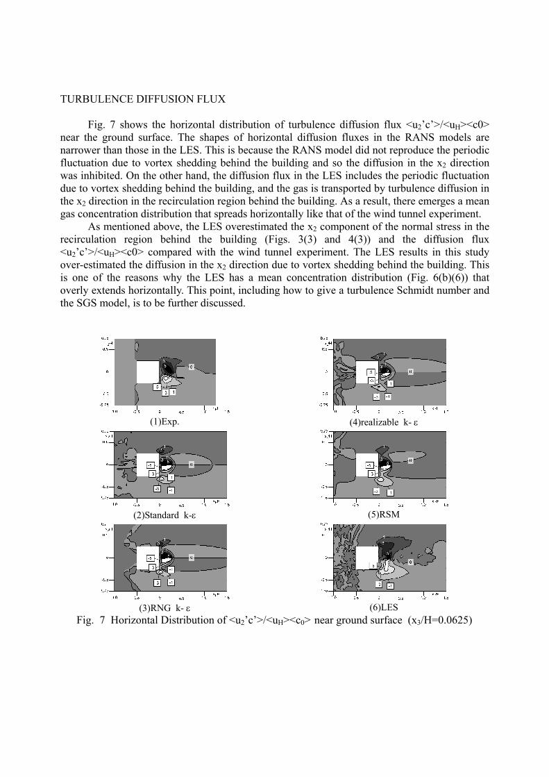
TURBULENCE DIFFUSION FLUX
Fig. 7 shows the horizontal distribution of turbulence diffusion flux <u2’c’>/<uH><c0> near the ground surface. The shapes of horizontal diffusion fluxes in the RANS models are narrower than those in the LES. This is because the RANS model did not reproduce the periodic fluctuation due to vortex shedding behind the building and so the diffusion in the x2 direction was inhibited. On the other hand, the diffusion flux in the LES includes the periodic fluctuation due to vortex shedding behind the building, and the gas is transported by turbulence diffusion in the x2 direction in the recirculation region behind the building. As a result, there emerges a mean gas concentration distribution that spreads horizontally like that of the wind tunnel experiment.
As mentioned above, the LES overestimated the x2 component of the normal stress in the recirculation region behind the building (Figs. 3(3) and 4(3)) and the diffusion flux <u2’c’>/<uH><c0> compared with the wind tunnel experiment. The LES results in this study over-estimated the diffusion in the x2 direction due to vortex shedding behind the building. This is one of the reasons why the LES has a mean concentration distribution (Fig. 6(b)(6)) that overly extends horizontally. This point, including how to give a turbulence Schmidt number and the SGS model, is to be further discussed.
(1)Exp. (4)realizable k- ε
(2)Standard k-ε (5)RSM
(3)RNG k- ε (6)LES
Fig. 7 Horizontal Distribution of <u2’c’>/<uH><c0> near ground surface (x3/H=0.0625)

CONCLUSION
The flows and concentration fields around a building placed within the boundary layer were analyzed using several revised k-ε models, the RSM and the LES. The calculation results were compared with those of wind tunnel experiments, focusing on the weak wind region behind the building. (1) The LES reproduced the periodic fluctuation due to vortex shedding behind the building, which significantly improved the prediction accuracies of the size of the recirculation region behind the building, the mean wind velocity distribution in the weak wind region in the vicinity of the ground surface, and the normal stresses compared with RANS models. (2) Periodic fluctuations due to the vortex shedding have a significant influence on the diffusion field as well as on the flow field. In the LES, the mean concentration distributions closely corresponded to those in the experiment because the periodic fluctuations were reproduced. In the RANS models, on the other hand, the periodic fluctuations were not reproduced and the mean concentration and the turbulence diffusion flux <u2'c'> did not sufficiently spread in the x2 direction. Symbols
xi : three components of space coordinates (i = 1,2,3: streamwise, lateral, vertical) ui : three components of velocity vector f : instantaneous value of a quantity
<f> : time-averaged value of f H : building height (0.2 m)
<uH> : <u1> value at inflow of computational domain at height H q : gas emission amount
<C0> : reference gas concentration (q/<uH>H2) Acknowledgements
This computation was conducted as one of the projects entitled “WG for prediction of the Air Ventilation and Diffusion in Urban Areas” of the outdoor environment prediction and assessment subcommittee of the Architectural Institute of Japan. The WG members provided us with helpful advice and support. In addition, Ms. K. Horikawa and Mr. T. Deguchi, student of Tokyo Polytechnic University, assisted us in writing this manuscript. We would like to express our heartfelt thanks to them.
This study was partially funded by the Ministry of Education, Culture, Sports, Science and Technology, Japan, Grant-in-Aid for Scientific Research (B), 19360265 and the 21st Century Center of Excellence Program of Tokyo Polytechnic University. REFERENCES Mochida, A., Tominaga, Y. et al. (2006), “AIJ Guideline for Practical Applications of CFD to
Wind Environment around Buildings’’, Proceedings of The 4th International Symposium on Computational Wind Engineering, 533-536
Architectural Institute of Japan (2007), “Guidebook for Practical Applications of CFD to Pedestrian Wind Environment around Buildings”

Murakami, S, Mochida, A. and Hayashi, Y. (1990), “Examining the k-ε model by means of a wind tunnel test and large-eddy simulation of the turbulence structure around a cube”, Journal of Wind Engineering and Industrial Aerodynamics 35, 87-100
Durbin, P. A. (1996), Technical Note: “On the k-ε stagnation point anomaly”, Int. J. Heat and Fluid Flow, 17, 89-90
Tominaga, Y., Mochida, A., Shirasawa, T., Yoshie, R., Kataoka, H., Harimoto, K. and Nozu, T. (2004), “Cross Comparisons of CFD Results of Wind Environment at Pedestrian Level around a High-rise Building and within a Building Complex”, Journal of Asian Architecture and Building Engineering, 3(1), 63-70
Tominaga, Y, Mochida, A., Murakami, S. and Sawaki, S. (2008), “Comparison of various revised k-ε models and LES applied to flow around a high-rise building model with 1:1:2 shape placed within the surface boundary layer”, Journal of Wind Engineering and Industrial Aerodynamics 96, 4, 389-411
Tominaga, Y., Murakami, S., and Mochida, A. (1997), “CFD prediction of gaseous diffusion around a cubic model using a dynamic mixed SGS model based on composite grid technique”, Journal of Wind Engineering and Industrial Aerodynamics 67&68, 827-841
H.Tanaka, R.Yoshie, Cheng-Hu Hu (2006), ”Uncertainty in Measurements of Velocity and Concentration around a Building”, The 4th International Symposium on Computational Wind Engineering, 549-552
Kirkup, L. and Frenkel, B.(2006), “An introduction to uncertainty in measurement”, Cambridge University press
Yakhot. Y, Orszag, S. A., Thangam, S., Gatski, T. B. and Speziale, C. G. (1992), “Development of turbulence models for shear flows by a double expansion technique”, Phys. Fluids A 4 1510-1520
Shih, T.-H., Liou, W. W.,Shabbir, A., Yang, Z. and Zhu, J. (1995) , “A New k-² Eddy-Viscosity Model for High Reynolds Number Turbulent Flows - Model Development and alidation”, Computers Fluids, 24(3):227–238
Gibson, M. M., and Launder, B. E. (1978) , “Ground Effects on Pressure Fluctuations in the Atmospheric Boundary Layer”, J. Fluid Mech., 86:491–511, 1978.
Tominaga, Y., Mochida, A., and Murakami, S., (2003), “Large eddy simulation of flowfield around a high-rise building”, Conference Preprints of 11th International Conference on Wind Engineering, Lubbock, Texas, U.S.A., 2, 2543-2550
Kataoka, H. and Mizuno, M., (2002), “Numerical flow computation around aeroelastic 3D square cylinder using inflow turbulence”, Wind & Structures, 5(2-4) 379-392
Werner, H. and Wengle, H. (1991), “Large-eddy simulation of turbulent flow over and around a cube in plate channel: Proceedings 8th Symposium on Turbulent shear Flows”, 19-4, 155-158
Leonard, B.P. (1981), “A survey of finite differences with upwinding for numerical modeling of the incompressible convective diffusion equation”, Computational Techniques in Transient and turbulent Flow, 2, Pineridge Press

高層密集市街地における建物群の形態が歩行者レベルの風速・気温分布に与える影響 EXPERIMENTAL STUDY ON AIR VENTILATION IN
A BUILT-UP AREA WITH CLOSELY-PACKED HIGH-RISE BUILDINGS
義江龍一郎*1, 田中英之*2, 白澤多一*2, 小林剛*3 Ryuichiro YOSHIE, Hideyuki TANAKA, Taichi SHIRASAWA and Tsuyoshi KOBAYASHI
In this study, we investigated characteristics of air ventilation and thermal environment in a built-up area with closely-packed high-rise buildings by wind tunnel experiments. The objectives of this study were to grasp the situation of the air ventilations in the extremely dense city, and to assess the influence of forms of building groups on the air ventilation. As the experimental results, spatial average of wind velocity ratios at pedestrian level could be expressed by vertical average of gross building coverage ratio, and the height variation of buildings was very effective for improving the air ven-tilation and the thermal environment in this dense area.
Keywords : Area with closely-packed high-rise buildings, Air ventilation, Floor area ratio, Building coverage ratio, Height variation 高層密集市街地,風通し,容積率,建蔽率,建物高さのバリエーション
1.はじめに
狭い土地に人口が集中し,高層ビルが密集して建ち並ぶ香港では,
都市の風通しの悪さやエネルギー消費量の急速な増加によって,ヒ
ートアイランド現象や汚染物質の滞留が深刻な問題となっている。
こうした問題に対処するために,香港政府都市計画局では「Air
Ventilation Assessment System (AVAS):都市通風換気アセスメント
システム」の制定を目指している。AVAS のコンサルタントチーム
は,”The more air ventilation, the better”をスローガンとして,風通し
をよくするための都市計画のガイドラインや,開発行為に対する事
前影響評価方法などの検討を開始したところである。都市の風通し
を改善するための方策としては,水平方向の風を都市領域内に引き
入れること,すなわち地表付近の「水平方向の風の道」を確保する
ことに焦点が当てられがちである。主風向に対する建物の見つけ面
積を少なくするとスコアが高くなる建築物総合環境性能評価システ
ム CASBEE-HI もその一例である。確かにグロス建蔽率を小さくす
ることで市街地の風通しが改善されるとの報告もあり 1),2),街路幅
や空き地を広くとって建蔽率を低減させることは,ヒートアイラン
ドの緩和策として極めて有効であることには違いない。しかし,香
港のような高層密集市街地では,建蔽率を大きく低減させることは
困難であり,建物群の形態を工夫することで上空の涼風を都市キャ
ノピー内に導くこと,すなわち「鉛直方向の風の道」を確保するこ
とが重要であると筆者らは考える。なお,ここで「鉛直方向の風の
道」とは,建物周辺に生じる鉛直方向の平均流れ(移流)や鉛直方向の
乱流拡散によって,上空の新鮮な冷気流が地表付近まで輸送され,
また地表付近で発生する汚染物質や熱が上空に排出される効果(経
路)と定義する。
本研究では AVAS 制定のための基礎情報を提供するために,日本
よりはるかに高密度な香港の高層密集市街地での風通しの現状を把
握するとともに,容積率や建蔽率,建物高さのバリエーション等に
よる建物群の形態の違いが,街区内の歩行者レベルにおける風速・
気温分布に与える影響を風洞実験により調査した。
2.実験概要
2.1 比較する建物群形態
香港において最も密集した高層市街地の一つである旺角
(Mong-Kok)の市街地,約 600m 四方の範囲(図 1)を参考に,街区を縮
尺 1/600 で表 1 中のパース図のようにモデル化した。旺角の建物群
を忠実に再現せずに,このような単純なモデル化をした理由は,こ
の実験の目的が,旺角を対象としたケーススタディではなく,建物
群の形態が街区内の通風性状に及ぼす影響に関して何らかの普遍的
な知見を得ることにあるためである。
表 1 に風洞実験で用いた模型の特徴を示す。基準ケースとして,
本稿は 2007 年度日本建築学会大会学術講演概要集に掲載されたもの 5)に新しい知見を加え,再構成したものである。 *1 東京工芸大学工学部建築学科 教授・博士(工) Prof., Department of Architecture, Faculty of Eng., Tokyo Polytechnic University, Dr. Eng. *2 東京工芸大学大学院工学研究科 研究員・博士(工) Researcher, Graduate School of Eng., Tokyo Polytechnic University, Dr. Eng. *3 東京工芸大学大学院工学研究科 大学院生 Graduate Student, Graduate School of Eng., Tokyo Polytechnic University
図 1 モデル化範囲 (香港,旺角の中心市街地)
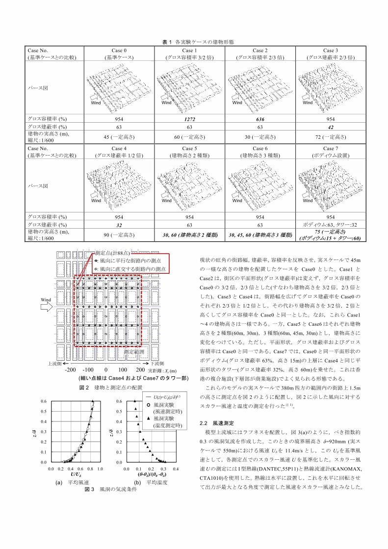
現状の旺角の街路幅,建蔽率,容積率を反映させ,実スケールで 45m
の一様な高さの建物を配置したケースを Case0 とした。Case1 と
Case2 は,街区の平面形状(グロス建蔽率)は変えず,グロス容積率を
Case0 の 3/2 倍,2/3 倍とした(すなわち建物高さを 3/2 倍,2/3 倍と
した)。Case3 と Case4 は,街路幅を広げてグロス建蔽率を Case0 の
それぞれ 2/3 倍と 1/2 倍とし,その代わり建物高さを 3/2 倍,2 倍と
高くしてグロス容積率を Case0 と同一とした。なお,これら Case1
~4 の建物高さは一様である。一方,Case5 と Case6 はそれぞれ建物
高さを 2 種類(60m, 30m),3 種類(60m, 45m, 30m)とし,建物高さに
変化をつけている。ただし,平面形状,グロス建蔽率およびグロス
容積率は Case0 と同一である。Case7 では,Case0 と同一平面形状の
ポディウム(グロス建蔽率 63%,高さ 15m)の上層に Case4 と同じ平
面形状のタワー(グロス建蔽率 32%,高さ 60m)を乗せた。これは香
港の複合施設(下層部が商業施設)でよく見られる形態である。
これらのモデルの実スケールで 380m 四方の範囲内の街路上 1.5m
の高さに測定点を図 2 のように配置し,図 2 に示した風向に対する
スカラー風速と温度の測定を行った注 1)。
2.2 風速測定
模型上流域にはラフネスを配置し,図 3(a)のように,べき指数約
0.3 の風洞気流を作成した。このときの境界層高さ δ=920mm (実ス
ケールで 550m)における風速 Uδを 11.4m/s とし,この Uδを基準風
速として,各測定点でのスカラー風速 U を基準化した。スカラー風
速 Uの測定には I型熱線(DANTEC,55P11)と熱線流速計(KANOMAX,
CTA1010)を使用した。熱線は水平に設置し,これを水平に回転させ
て出力が最大となる角度で測定した風速をスカラー風速とみなした。
表 1 各実験ケースの建物形態 Case No. (基準ケースとの比較)
Case 0 (基準ケース)
Case 1 (グロス容積率 3/2 倍)
Case 2 (グロス容積率 2/3 倍)
Case 3 (グロス建蔽率 2/3 倍)
パース図
グロス容積率 (%) 954 1272 636 954 グロス建蔽率 (%) 63 63 63 42 建物の実高さ (m), 縮尺:1/600 45 (一定高さ) 60 (一定高さ) 30 (一定高さ) 72 (一定高さ)
Case No. (基準ケースとの比較)
Case 4 (グロス建蔽率 1/2 倍)
Case 5 (建物高さ 2 種類)
Case 6 (建物高さ 3 種類)
Case 7 (ポディウム設置)
パース図
グロス容積率 (%) 954 954 954 954 グロス建蔽率 (%) 32 63 63 ポディウム:63, タワー:32 建物の実高さ (m), 縮尺:1/600 90 (一定高さ) 30, 60 (建物高さ 2 種類) 30, 45, 60 (建物高さ 3 種類) 75 (一定高さ)
(ポディウム:15 + タワー:60)
(細い点線は Case4 および Case7 のタワー部)
図 2 建物と測定点の配置
(a) 平均風速 (b) 平均温度 図 3 風洞の気流条件
Wind Wind Wind Wind
Wind Wind Wind Wind
7 6 7 6 7 6 7 6 7 6 7 6 7 6 7 6 7 6 7 6 7 6 7 6
7 6 7 6 7 6 7 6 7 6 7 6 7 6
7 6 7 6 7 6 7 6 7 6 7 6 7 6
7 6 7 6 7 6 7 6 7 6 7 6 7 6
7 6 7 6 7 6 7 6 7 6 7 6 7 6
7 6 7 6 7 6 7 6 7 6 7 6 7 6 7 6 7 6 7 6 7 6 7 6
7 6 7 6 7 6 7 6 7 6 7 6 7 6 7 6 7 6 7 6 7 6 7 6
7 6 7 6 7 6 7 6 7 6 7 6 7 6 7 6 7 6 7 6 7 6 7 6
7 6 7 6 7 6 7 6 7 6 7 6 7 6 7 6 7 6 7 6 7 6 7 6
測定範囲
Wind
7 6
7 6: 風向に平行な街路内の測点
: 風向に直交する街路内の測点
測定点(計88点)
-200 -100 0 100 200下流側上流側
実距離 : Xr (m)2001000-100-200
0.0
0.1
0.2
0.3
0.4
0.5
0.6
0.0 0.2 0.4 0.6 0.8 1.0
z /δ
U/Uδ
0.0
0.1
0.2
0.3
0.4
0.5
0.6
0.0 0.1 0.2 0.3 0.4
z /δ
(θ-θδ)/(θ0 -θδ)
風洞実験
(温度測定時)
(風速測定時)風洞実験
U(z)=Uδ(z/δ)0.3

このように熱線を水平に設置した理由は,鉛直方向成分を含むスカ
ラー風速を測定するためである。なお,各ケースの最大建物高さで
の風速から算出したレイノルズ数(Re数)は Re≧1.7 x10⁴である。
2.3 温度測定
温度測定時の風洞気流は,境界層高さの風速を Uδ=1.9m/s とし,
風速測定時と同程度のべき指数となるように作成した(図 3(a))。そ
の際,境界層高さの気流温度 θδ および床面温度 θ0をそれぞれ 7.6 oC
と 45.3oCとして,図 3(b)のように気流温度を不安定成層条件とした。
このときの Re数は Re≧3.4 x10³ 注 2),バルクリチャードソン数(Rb数)
は Rb= -0.23 である注 3)。気流温度 θは DANTEC 社製の冷線(55P31)
と抵抗温度計(90C20)を用いて測定し,θδおよび θ0で基準化した。
3.実験結果
3.1 建物群の形態が風通しに及ぼす影響
(1) 容積率の影響(Case0 と Case1,2 の比較)
歩行者レベル高さ 1.5m の風速比 U/Uδ およびその空間平均値
<U/Uδ>を,風向に平行な街路内(図 4(a))と直交する街路内(図 4(b))
の測定点で分けて示す。図 4(c)では,これら全測定点の風速比から
算出した空間平均値を示すとともに,その確率密度分布を Weibll
分布で近似して各ケースの通風性能を特徴付けている。また,その
近似精度の指標として近似標準誤差 SE注 4)も図 4(c)中に併せて示す。
風向に平行な街路内(図 4(a))では,グロス容積率が大きいほど,
その風速比は街区上流側で大きく,下流側では小さい。これは,風
上側では建物の高層化に伴って風上端の高層建物間の縮流が強くな
り,風下側では抵抗の増加により流れが遅くなっているものと考え
られる。風向に直交する街路内(図 4(b))では,いずれのケースも風
向に平行な街路内(図 4(a))と比べて風速はかなり低い。また,グロ
ス容積率が大きいほど風速比がやや小さくなる傾向を示している。
図 4(c)の確率密度分布では,グロス容積率が大きいほど風速分布
の幅が広がっているが,街区全体では風速比の増減が相殺されたた
め,各ケース間の空間平均値に大きな差は生じていない。
(2) 建蔽率の影響(Case0 と Case3,4 の比較)
建蔽率による影響も前記の容積率の影響(図 4(a)~(c))と同様に整
理して図 5 に示す。
図 5(a)より,風向に平行な街路内全域で,グロス建蔽率が 2/3 倍,
1/2 倍と小さくなるに従い,風速比の空間平均値は 1.6 倍,2 倍と大
きく改善されている。風向に直交する街路内(図 5(b))でも,グロス
建蔽率が小さいほど風速比が大きいが,風向に平行な街路(図 5(a))
で見られたほどの効果はない。図 5(c)の確率密度分布に示すように,
街区全体では Case3,4 のピーク位置が高風速側に大きく移動し,街
路幅を Case0 の 2 倍とした Case4 では,その空間平均値も Case0 の
ほぼ 2 倍となっている。
久保田らは,実在する日本の中・高層街区を対象に,グロス建蔽
率と地上高さ 1.5m における平均風速比の関係を図 6 のように整理
している 1)。現状の旺角のグロス建蔽率を反映させた Case0 は久保
田らによる日本の中・高層街区と比べるとはるかに風通しが悪い。
久保田らの実験は,建物高さのバリエーションがそれほど大きくな
い地域を対象としたものであるが,建物高さが一様である本実験の
(a) 風向に平行な街路内の風速比 (b) 風向に直交する街路内の風速比 (c) 風速比の確率密度分布
図 4 グロス容積率の影響
(a) 風向に平行な街路内の風速比 (b) 風向に直交する街路内の風速比 (c) 風速比の確率密度分布
図 5 グロス建蔽率の影響
0
0.1
0.2
0.3
0.4
-200 -100 0 100 200
風速
比U
/Uδ
Xr (m)
Case1(容積率3/2倍) : 0.14Case0(基準ケース) : 0.12Case2(容積率2/3倍) : 0.11
0
5
10
0 0.1 0.2 0.3 0.4 0.5
確率
密度
f (%
)
風速比 U/Uδ
Case1 : 0.11Case0 : 0.10Case2 : 0.09
Case No. : 空間平均値
U1.5 /Uδ =0.27(建物がない場合の風速比)
0
0.1
0.2
0.3
0.4
-200 -100 0 100 200
風速
比U
/Uδ
Xr (m)
Case1(容積率3/2倍) : 0.05Case0(基準ケース) : 0.06Case2(容積率2/3倍) : 0.06
Case No. : 空間平均値
,SE =1.7,SE =2.1,SE =2.0
空間
平均値,Case No.:近似標準
誤差(%)
0
0.1
0.2
0.3
0.4
-200 -100 0 100 200
風速
比U
/Uδ
Xr (m)
Case0(基準ケース) : 0.12Case3(建蔽率2/3倍) : 0.19Case4(建蔽率1/2倍) : 0.24
0
0.1
0.2
0.3
0.4
-200 -100 0 100 200
風速
比U
/Uδ
Xr (m)
Case0(基準ケース) : 0.06Case3(建蔽率2/3倍) : 0.07Case4(建蔽率1/2倍) : 0.08
Case No. : 空間平均値Case No. : 空間平均値
0
5
10
0 0.1 0.2 0.3 0.4 0.5
確率
密度
f(%
)
風速比 U/Uδ
Case0 : 0.10Case3 : 0.16Case4 : 0.19
U1.5 /Uδ =0.27(建物がない場合の
風速比)
,SE =2.1,SE =2.2,SE =2.4
空間
平均値,Case No.:近似標準
誤差(%)

Case0 と Case3,Case4 の結果は,久保田らが求めた近似直線の延長
線上にあることがわかる。また,これらのケースとは大きくグロス
容積率の異なる Case1 と Case2 の平均風速比は,Case0 の平均風速
比と大差ないため,やはり同じ近似直線上に分布している。このこ
とから,本実験対象のように極度に密集した Case0~Case4 のような
街区であってもその平均風速比はグロス建蔽率によって評価でき,
グロス容積率による影響は小さいことが明らかとなった。また,久
保田らが対象とした実在街区のグロス建蔽率とグロス容積率はそれ
ぞれ 10~30%と 69~171%,本実験ではそれぞれ 32~63%と 636~
1272%であり,非常に幅広い範囲の建物密度にわたって,都市の平
均的な風通しが,このように一つの直線で整理できることは,都市
再開発や大規模な開発行為の基本計画を考える上で有用な結果であ
ると思われる。
(3) 建物高さのバリエーションの影響(Case0 と Case5,6 の比較)
建物高さのバリエーションによる影響を図 7 に示す。図 7(a),(b)
より,建物高さに変化がある Case5,6 では,多くの測定点で風速比
は Case0 よりも高くなっている。特に風向に直交する街路内の空間
平均風速比は Case0 の 0.06 から 0.11(Case5),0.15(Case6)まで増加
しており,前述のグロス建蔽率を低減させた場合の 0.07(Case3),
0.08(Case4)と比べても大きく改善されている。また,Case5,6 では,
風向に平行な街路内の下流域でも風速が他のケースよりも高くなっ
ていることがわかる。このように建物高さに変化がある場合には,
建物背後や街区下流域でも通風性状が大きく改善されている。また,
図 7(c)より,その確率密度は建物高さのバリエーションが増えるに
従って高風速域にまで分布が拡がり,街区全体の空間平均風速比も
高くなっている。
(4) ポディウムの影響(Case0 と Case7 の比較)
図 8(a),(b)でポディウムを有する Case7 の風速比を基準ケースで
ある Case0 の結果と比較した。図 8(a)より,風向に平行な街路内で
は,Case7 の風速比は街区上流側で大きく下流側ほど小さい。また
その風速比の空間平均値 0.20 は Case0 の空間平均値に比べると大き
く改善されており,グロス建蔽率を下げた Case3,4 の通風性状(図
5(a))と同じ傾向を示している。図 8(b)の風向に直交する街路内では,
建物高さを変化させた Case5,6(図 7(b))ほどではないがグロス建蔽
率を下げた Case3,4(図 5(b))よりもその風通しは改善されている。
図 8(c)には Case0 と Case7 の確率密度とともに Case4 と Case6 の結
果も併せて示す。Case7 の確率密度は Case4(グロス建蔽率 1/2 倍)と図 6 グロス建蔽率と風速比の関係
(a) 風向に平行な街路内の風速比 (b) 風向に直交する街路内の風速比 (c) 風速比の確率密度分布
図 7 建物高さのバリエーションの影響
(a) 風向に平行な街路内の風速比 (b) 風向に直交する街路内の風速比 (c) 風速比の確率密度分布
図 8 ポディウムの影響
y = -0.002x + 0.273相関係数:R = 0.85
0
0.05
0.1
0.15
0.2
0.25
0 20 40 60 80
風速
比の
空間
平均
値<U
/Uδ>
グロス建蔽率 (%)
Case0 ダミー
Case1 Case2Case3 Case4 K ダミー日本の中・高層街区(久保田 et al.)
0
0.1
0.2
0.3
0.4
-200 -100 0 100 200
風速
比U
/Uδ
Xr (m)
Case0(基準ケース) : 0.12Case5(建物高さ2種類) : 0.14Case6(建物高さ3種類) : 0.17
0
0.1
0.2
0.3
0.4
-200 -100 0 100 200
風速
比U
/Uδ
Xr (m)
Case0(基準ケース) : 0.06Case5(建物高さ2種類) : 0.11Case6(建物高さ3種類) : 0.15
0
5
10
0 0.1 0.2 0.3 0.4 0.5
確率
密度
f (%
)
風速比 U/Uδ
Case0 : 0.10Case5 : 0.13Case6 : 0.16
Case No. : 空間平均値Case No. : 空間平均値
U1.5 /Uδ=0.27(建物がない場合の
風速比)
,SE =2.1,SE =1.6,SE =1.8
空間
平均値,Case No.:近似標準
誤差(%)
0
0.1
0.2
0.3
0.4
-200 -100 0 100 200
風速
比U
/Uδ
Xr (m)
Case0(基準ケース) : 0.12Case7(ポディウム付) : 0.20
0
0.1
0.2
0.3
0.4
-200 -100 0 100 200
風速
比U
/Uδ
Xr (m)
Case0(基準ケース) : 0.06Case7(ポディウム付) : 0.09
0
5
10
0 0.1 0.2 0.3 0.4 0.5
確率
密度
f(%
)
風速比 U/Uδ
Case0 : 0.10Case4 : 0.19Case6 : 0.16Case7 : 0.17
U1.5 /Uδ =0.27(建物がない場合の
風速比)
Case No. : 空間平均値 Case No. : 空間平均値
,SE =2.1,SE =2.4,SE =1.8,SE =1.8
空間
平均値,Case No.:近似標準
誤差(%)

Case6(建物高さ 3 種類)の間の傾向を示し,その空間平均風速比も
Case4 に次いで高い結果となっている。このようにタワー状の高層
建物の下部にポディウムがあっても,歩行者レベルの風通しに対し,
それほど悪影響を及ぼしておらず,Case4 と比べてもそれほど風通
しは悪くなっていない。
(5) 高さ方向平均グロス建蔽率による風通しの評価
(2)で述べたように,建物高さがほぼ一様であるような場合(Case0
~4)はグロス建蔽率によって街区内の平均的な風通しを評価するこ
とができた。しかし,建物高さに変化がある場合(Case5,6)やポデ
ィウムの上層にタワーを設置する場合(Case7)のように,街区内の上
下方向で建物の空間に占める割合が大きく変わる場合には,歩行者
レベルのグロス建蔽率が同じであっても,その平均風速比は久保田
らの近似直線の上方に位置している(図 9)。このように街区の風通し
を評価するためには,歩行者レベルのグロス建蔽率だけではなく,
街区上層の形態も考慮する必要がある。そこで,以下の高さ方向平
均グロス建蔽率を用いて街区の平均的な風通しを評価することを試
みた。
1 (1)
ここで,λac :高さ方向平均グロス建蔽率
hmax :街区内の最高建物高さ
λ(z) :高さ z における建物群水平断面積が街区全体の面積
に占める割合
各ケースの空間平均風速比をこの高さ方向平均グロス建蔽率で整
理した結果を図 10 に示すが,すべてのケースの空間平均風速比が 1
本の直線上にほぼのっている。このように街区内の上下方向で大き
く建物群の形態が変わる場合であっても,提案した高さ方向平均グ
ロス建蔽率を一つの指標とすれば,歩行者レベルの平均的な風通し
の程度を普遍的に評価できる可能性がある。
3.2 建物群の形態が気流温度に及ぼす影響
測定した気流温度 θ については,境界層高さ温度 θδとの差 θ-θδを床面温度と境界層高さ温度の差 θ0-θδ で基準化した温度比
(θ-θδ)/(θ0-θδ)として整理した。図 9 で風速比の空間平均値が高かっ
た Case4,Case6,Case7 を取り上げ,それらの温度比を Case0(基準
ケース)と比較した結果を図 11~13 に示す。図 14 には,これらの全
測定点の温度比から算出した空間平均値と Weibll 分布で近似した
確率密度分布を示し,図 16 に,全ケースの温度比の空間平均値と高
さ方向平均グロス建蔽率の関係を示す。
(1) 建蔽率の影響
Case4 の風洞気流に平行な街路内(図 11(a))では,街路幅が 2 倍と
なったことによる「水平方向の風の道」の効果のため,街区上流側
で気流温度が Case0 よりも大きく下がっている。しかし,街区の下
流側ほど気流温度は上がる傾向にあり,そこでは Case0 からの改善
効果は小さい。風洞気流に直交する街路内(図 11(b))でも,Case4 の
気流温度は低くなっている。また,図 16 のように Case0 と Case1~
Case4 は同一直線上にあるため,街区内の気流温度性状もグロス建
蔽率(建物高さが一定の場合,高さ方向平均グロス建蔽率はグロス建
蔽率と同値)で整理でき,グロス容積率にはほとんど依存しないこと
がわかる。
(2) 建物高さのバリエーションの影響
Case6(図 12)は,Case4,Case7 とは異なった気流温度分布である。
特に,街区の下流域や風洞気流に直交する街路内(図 12(b))での気流
温度の改善傾向が Case4,Case7 に比べて大きい。確率密度分布を示
した図 14 においても,Case6 の空間平均温度は Case4 と同程度とな
っているが,その確率密度は Case4 よりも低温度側に広く分布して
いる。ここで,街路内の空間平均温度が低く,同程度であった Case4
と Case6 の風速比と温度比の関係と相関係数 R を図 15 に示す。風
洞気流に平行な街路内(図 15(a))では,Case4,Case6 ともに負の相関
を持っている。すなわち,風速が高いほど気流温度は低くなってい
る。しかし,風洞気流に直交する街路内(図 15(b))では,Case6 の風
速比と気流温度にはほとんど相関が見られない。このように建物高
さにバリエーションがある場合では,風向に直交する街路内や街区
の下流域のような弱風域であっても気流温度が下がっており,上空
の冷たい気流が鉛直方向の移流または乱流拡散によって地上付近に
まで輸送されるとともに地表付近の熱が効果的に上空へと排出され
たと考えられる。また,図 10 の高さ方向平均グロス建蔽率と風速比
の関係と異なり,図 16 の Case5,6 の温度比は,建物高さが一定の
場合の高さ方向平均グロス建蔽率(グロス建蔽率)-温度比の直線の
下方にあり,街区の風通し以上に気流温度が改善されたことを示し
ている。このように建物高さにバリエーションがある場合は,グロ
ス建蔽率を下げて同程度の風通しを確保した場合よりも,街区内の
図 9 グロス建蔽率と風速比の関係(建物高さを変化させた効果)
図 10 高さ方向平均グロス建蔽率と風速比の関係
0
0.05
0.1
0.15
0.2
0.25
0 20 40 60 80
風速
比の
空間
平均
値<U
/Uδ>
グロス建蔽率 (%)
Case0 Case1Case2 Case3Case4 Case5 Case6 Case7K日本の中・高層街区(久保田 et al.)
0
0.05
0.1
0.15
0.2
0.25
0 20 40 60 80
風速
比の
空間
平均
値<U
/Uδ>
高さ方向平均グロス建蔽率 (%)
Case0 Case1Case2 Case3Case4 Case5 Case6 Case7K日本の中・高層街区(久保田 et al.)

気流温度がより改善されており,ヒートアイランド現象に対して
「鉛直方向の風の道」を考慮することの重要性が確認された。実在の
都市は容積率等の制限から,久保田らが対象とした測定ケース 1),2)
のように建物高さが一定に近い場合が多いが,今後都市の換気能力
を向上させるためには建物高さにバリエーションを与えることも一
つの施策として有効であると考える。この効果は香港のように密集
した都市においては特に大きいと推察する。
(3) ポディウムの影響
Case7(図 13)では,街区上方(15m 以上の高さ)の見つけ面積を小さ
くしているため,気流温度は Case0 よりも改善されている。しかし,
歩行者レベルのグロス建蔽率は Case0 と変わっていないため,Case4
ほどの改善効果はない。図 10 では,ポディウムを有する Case7 の平
均風速比は Case4 に次いで高い結果となっているにもかかわらず,
(a) 風向に平行な街路内の温度比 (a) 風向に平行な街路内の温度比 (a) 風向に平行な街路内の温度比
(b) 風向に直交する街路内の温度比 (b) 風向に直交する街路内の温度比 (b) 風向に直交する街路内の温度比 図 11 グロス建蔽率の影響 図 12 建物高さのバリエーションの影響 図 13 ポディウムの影響
(a) 風向に平行な街路内の温度比 (b) 風向に直交する街路内の温度比
図 14 温度比の確率密度分布 図 15 風速比と温度比の相関
図 16 高さ方向平均グロス建蔽率と温度比の関係
0.2
0.4
0.6
0.8
-200 -100 0 100 200
温度
比(θ
-θ δ
)/(θ 0
-θ δ
)
Xr (m)
Case0(基準ケース) : 0.64
Case7(ポディウム付) : 0.580.2
0.4
0.6
0.8
-200 -100 0 100 200
温度
比(θ
-θ δ
)/(θ 0
-θ δ
)
Xr (m)
Case0(基準ケース) : 0.64
Case4(建蔽率1/2倍) : 0.480.2
0.4
0.6
0.8
-200 -100 0 100 200
温度
比(θ
-θ δ
)/(θ 0
-θ δ
)
Xr (m)
Case0(基準ケース) : 0.64
Case6(建物高さ3種類) : 0.53
Case No. : 空間平均値Case No. : 空間平均値
Case No. : 空間平均値
0.2
0.4
0.6
0.8
-200 -100 0 100 200
温度
比(θ
-θ δ
)/(θ 0
-θ δ
)
Xr (m)
Case0(基準ケース) : 0.68
Case7(ポディウム付) : 0.620.2
0.4
0.6
0.8
-200 -100 0 100 200
温度
比(θ
-θ δ
)/(θ 0
-θ δ
)
Xr (m)
Case0(基準ケース) : 0.68
Case4(建蔽率1/2倍) : 0.610.2
0.4
0.6
0.8
-200 -100 0 100 200
温度
比(θ
-θ δ
)/(θ 0
-θ δ
)
Xr (m)
Case0(基準ケース) : 0.68
Case6(建物高さ3種類) : 0.49
Case No. : 空間平均値
Case No. : 空間平均値
Case No. : 空間平均値
0
5
10
15
20
0.2 0.4 0.6 0.8 1
確率
密度
f(%
)
温度比 (θ- θδ)/(θ0- θδ)
Case0 : 0.65Case4 : 0.52Case6 : 0.52Case7 : 0.59
θ1.5- θδθ0 - θδ
=0.33
(建物がない
場合の温度比)
,SE =1.8,SE =2.8,SE =1.8,SE =2.2
空間
平均値,Case No.:近似標準
誤差(%)
0 0.1 0.2 0.3 0.4 0.5
風速比 U/Uδ
0.2
0.3
0.4
0.5
0.6
0.7
0.8
0 0.1 0.2 0.3 0.4 0.5
温度
比(θ-
θ δ)
/(θ 0
-θ δ
)
風速比 U/Uδ
Case4 : R=-0.81Case6 : R=-0.68
Case4 : R=-0.49Case6 : R=-0.01
Case4 (建蔽率1/2倍)
Case6 (建物高さ3種類)
0.4
0.45
0.5
0.55
0.6
0.65
0.7
0.75
0.8
0 20 40 60 80
温度
比の
空間
平均
値
< (θ-
θ δ)/(θ 0
-θ δ
)>
高さ方向平均グロス建蔽率 (%)
Case0 Case1
Case2 Case3
Case4 Case5
Case6 Case7

その平均気流温度は Case3~6 よりも悪い(図 16)。また,Case7 の温
度比の空間平均値は,図 16 のように高さ方向平均グロス建蔽率(グ
ロス建蔽率)-温度比の直線の上方にある。ポディウムがあっても風
通しはそれほど悪化しないものの(Case4と比べてもそれほど風通し
は悪くはないものの),地表付近の気流温度は悪化してしまうことが
わかる。これは,ポディウム高さが一定なので鉛直方向の移流また
は乱流拡散が促進されず,そのため上空の冷気流が地表付近まで効
果的に輸送されていないとともに,地表面付近の熱が排出されにく
いものと推測される。
4.結論
香港のような極度に密集した高層市街地を対象として,容積率や
建蔽率,建物高さのバリエーション等による建物群の形態の違いが,
街区内の歩行者レベルにおける風速・気温分布に与える影響を風洞
実験により調査した。この実験から得られた知見をまとめると以下
のようになる。
1) 香港の高層密集市街地の現状を反映させたケースでは,久保田
らによる日本の中・高層街区と比べて,はるかに風通しが悪いこ
とが明らかとなった。
2) 建物高さが一様である場合には,街区内歩行者レベルの平均風
速比は,グロス容積率には依らず,グロス建蔽率に依存してい
る。今回の実験により得られた平均風速比とグロス建蔽率の関
係は,久保田らが求めた関係式の延長線上にあり,非常に幅広
い範囲の建物密度(グロス建蔽率,グロス容積率)にわたって,
街区内歩行者レベルの平均風速比をグロス建蔽率で評価できる
ことが明らかとなった。
3) 建物高さにバリエーションがある場合には,特に建物背後や街
区下流域での風通しが大きく改善される。
4) 建物高さにバリエーションがある場合やポディウムがある場合
のように,街区内の上下方向で大きく建物群の形態が変わる場
合であっても,今回提案した高さ方向平均グロス建蔽率を一つ
の指標とすれば,歩行者レベルの平均風速比を普遍的に評価す
ることができる。
5) 建物高さにバリエーションがある場合は,グロス建蔽率を下げ
て同程度の風通しを確保した場合よりも,街区内の気流温度が
より改善されている。これは上空の冷たい気流が地上付近にま
で効果的に輸送されているためであり,ヒートアイランド現象
に対して「鉛直方向の風の道」を考慮することの重要性が確認さ
れた。
6) タワー状の高層建物の下部にポディウムがある場合,下層部の
グロス建蔽率が高くても歩行者レベルの風通しに対して,風通
しはそれほど悪化しないものの,気流温度は悪化している。
謝辞
村上周三教授(慶應大学),持田灯教授(東北大学),Edward Ng 教授
(香港中文大学)からは本研究を実施するきっかけを与えて頂くとと
もに,実験ケースの設定にあたり貴重なご助言を頂いた。また,本
論文の投稿にあたっては,匿名の査読者から大変有意義なご助言を
頂いた。ここに記して謝意を表す。なお,本研究の一部は東京工芸
大学 21 世紀 COE プログラムによる成果である。
注
注 1) Case0 の風洞実験では,8 風向に対して風速を測定した。図 17 に示した
風向別の風速比の空間平均値は,方位によって大きな差はない(0.09~
0.11)。また,図 18 には 8 風向すべての風速比データを用いて算出した確
率密度分布を示すとともに,1 風向のみ(西風)のデータから算出した確率
密度分布も併せて示す。結果として,8 風向と本報と同じ風向(西風)のみ
の確率密度分布にも大きな差はない。
図 17 8 風向別の風速比の
空間平均値 図 18 8 風向と 1 風向の確率密度分布の比較
注 2) 温度測定時の Re数は風速測定時の約 1/5 であったが,Townsend らの研
究 3)より Re数が十分に大きければ建物周りの流れの構造は相似になるこ
とや,Hoydysh らの研究 4)で Re≧3.4 x10³ であればストリートキャニオン
内の基準化されたスカラー量の分布に差がなくなることが明らかになっ
ている。今回の実験ではいずれの測定ケースにおいても Re≧3.4 x10³ を
満たしており,Re 数の違う流れ場での風速測定と温度測定の結果を関連
付けて検証することに問題はない。
注 3) 温度測定時の Rb 数は Rb=-0.23 で,極めて弱い不安定状態である。実際
の夏季弱風時とは相似になっていないため,温度に関しては実験ケース
間の相対比較のみを目的とした。
なお,Rb = gδ(θδ-θ0) /{(θmean +273)(Uδ 2)} (2)
ここで,Uδ :境界層高さ風速(Uδ =1.93 m/s),δ : 境界層高さ(δ =0.67 m),
θδ :境界層高さの気流温度(θδ =7.6 oC),
θ0 :床面温度(θ0 =45.3 oC),
θmean:境界層内の平均温度(θmean =16.1 oC)
注 4) 近似標準誤差 SE(%)の定義を以下に示す。
SE = ∑
(3)
ここで,r :残差,確率密度 f とその近似値 の差( = f - )
ν :自由度,データ数 n と近似係数の個数 m の差( = n - m )
参考文献
1) 久保田徹, 三浦昌生, 富永禎秀, 持田灯: 実在する 270m 平方の住宅地にお
ける地域的な風通しに関する風洞実験 建築群の配置・集合形態が地域
的な風通しに及ぼす影響 その 1, 日本建築学会計画系論文集, 第 529 号,
pp.109-116, 2000.3
2) 久保田徹, 三浦昌生, 富永禎秀, 持田灯: 風通しを考慮した住宅地計画のた
めの全国主要都市におけるグロス建蔽率の基準値 建築群の配置・集合
形態が地域的な風通しに及ぼす影響 その 2, 日本建築学会計画系論文集,
第 556 号, pp.107-114, 2002.6
3) A. A. Townsend: The structure of turbulent shear flow, Cambridge Univ.
Press, 1956
4) W. G. Hoydysh, Y. Ogawa, R. A. Griffiths: A scale model study of dispersion
of pollutant in street canyons, The 67th APCA, pp.74-157, 1974.6
5) 義江龍一郎, 田中英之, 白澤多一, 小林剛: 香港の高層密集市街地における
風通しに関する研究(その 1) 建蔽率と建物高さのバリエーション等が歩
行者レベルの風速・気温分布に及ぼす影響, 日本建築学会大会学術講演概
要集(D1), pp.745-746, 2007.8
0
0.1
0.2North
NE
East
SE
South
SW
West
NW
0.00 0.250.05 0.15 0.20
15
10
5
確率
密度
f(%
)
0
風速比 U/Uδ
0.10
(f =)Akx k ⎪⎩
⎪⎨⎧
⎜⎝⎛−exp
⎪⎭
⎪⎬⎫
⎟⎠⎞
k−1k
Uδ
UUδ
⎟⎠⎞U
⎜⎝⎛
Uδ
UUδ
⎟⎠⎞U
⎜⎝⎛
⎝ AUδ
UUδ
⎟⎠⎞U
⎜⎝⎛
,風向8 1.1=E S近似標準誤差
,(West)風向1 1.2=E S
(f =)Akx k ⎪⎩
⎪⎨⎧
⎜⎝⎛−exp
⎪⎭
⎪⎬⎫
⎟⎠⎞
k−1k
Uδ
UUδ
⎟⎠⎞U
⎜⎝⎛
Uδ
UUδ
⎟⎠⎞U
⎜⎝⎛
AUδ
UUδ
⎟⎠⎞U
⎜⎝⎛

逆流を伴う非等温流れ場における風速・温度・濃度の同時測定方法 TECHNIQUE FOR SIMULTANEOUSLY MEASURING FLUCTUATING CONCENTRATION,
VELOCITY AND TEMPERATURE IN NON-ISOTHERMAL FLOW
田中英之*1, 義江龍一郎*2, 白澤多一*1, 栗田剛*3, 小林剛*4 Hideyuki TANAKA, Ryuichiro YOSHIE, Taichi SHIRASAWA, Tsuyoshi KURITA and Tsuyoshi KOBAYASHI
In this study, we aimed to provide experimental data to validate CFD for pollutant diffusion around buildings in non-isothermal flow. We developed a system for simultaneously measuring fluctuating velocity, temperature and concentration. The system compensates for the contribution of temper-ature to output voltage of a split film with a cold wire. We made a calibrator for a split film for different temperatures and proposed calibration equa-tions for it, and it showed good performance. These equations can be used to simultaneously measure wind velocity and temperature around buildings in non-isothermal flow. We used a high speed flame ionization detector to measure concentration simultaneously with wind velocity and temperature, enabling us to provide turbulence statistics such as turbulent heat flux and turbulent concentration flux.
Keywords: Wind tunnel experiment, Non-isothermal flow, Flow around a building, Turbulent heat flux, Turbulent concentration flux 風洞実験,非等温流れ場,建物周辺気流,乱流熱フラックス,乱流濃度フラックス
1.はじめに
k-ε系のモデルを用いた CFD(Computational Fluid Dynamics)は,い
わゆるビル風のような強風問題の予測に盛んに使われるようになっ
てきており,「市街地風環境予測のための流体数値解析ガイドブッ
ク」1)が作成されるなど,既に実用化の段階に入っていると言っても
過言ではない。一方,近年ではヒートアイランド現象や大気汚染の
問題を CFD で予測・評価する研究事例も増えてきており 2), 3), 4)等,
この種の問題に対しても今後 CFD が有効かつ実用的な手段となる
ことが期待されている。ヒートアイランド現象や大気汚染の問題は,
建物後流域や都市キャノピー内のような弱風域でより深刻となるが,
こうした弱風域に対して k-ε 系のモデルでは風速の予測精度が悪い
ことが明らかとなっている 5)~8)。さらに弱風域では,日射や夜間放
射によって加熱または冷却された地表面や建物壁面から気流への対
流熱伝達及び,それに伴う浮力の影響が相対的に大きくなるため,
その影響は無視できぬものであると思われる。しかし,こうした非
等温弱風域の流れ場,温度場,拡散場に対する CFD の予測精度に関
しては未だ十分な検証はなされていない。その検証に際しては,平
均量だけではなく乱流統計量,特に乱流熱フラックスや乱流濃度フ
ラックスといった乱流拡散にかかわる統計量も実験結果と比較し,
熱や汚染物質の輸送構造の再現性をも確認することが望ましい。し
かし,建物後流域や都市キャノピー内等の非等温流れ場に関して,
CFD の検証に耐えうる熱フラックスや濃度フラックスを含む乱流
統計量を備えた詳細な実験データベースは筆者らの知り得る限り存
在しない。これらの乱流フラックスを求めるためには,風速と温度,
風速と濃度の同時測定が必要となる。風速と温度を同時測定する場
合,既往の研究では,気流温度の影響を受けない LDV(Laser Doppler
Velocimettry)を用いた測定例が多数報告されている例えば,9)。しかし,
LDV を使用してさらに濃度も同時に測定しようとした場合は,シー
ディング粒子が濃度の測定機器に悪影響を及ぼす可能性があるため,
風速と温度,濃度の同時測定は非常に困難である。一方で,X-wire
と Cold-wire を組み合わせて風速と温度を同時測定した実験例もあ
るが,それらの対象は,温度成層条件下での境界層 10), 11)や 2 次元丘
陵の逆流が生じていない領域 12)に限られている。これは X-wire が
大きな変動を伴った流れ場での正流と逆流の判別ができないためで
ある。このように測定が非常に困難な「逆流を伴う非等温流れ場」に
おいて風速,温度,濃度を同時に測定するためには,下記の点に留
意した測定システムを構築する必要がある。
・ 風速,温度,濃度の瞬時値の同時測定が可能である。
・ 正流と逆流を伴った大きな乱れを有する流れ場の測定が可能
である。
・ 大きな温度変動のある流れ場で適切な温度補償が可能である。
そこで,著者らは逆流の測定が可能な Split-film を用い,Cold-wire
と高速 FID(水素炎式高速炭化水素計)を組み合わせた測定システム
を開発し,風速,温度,濃度の同時測定を可能とした。本報では,
Split-film と Cold-wire の較正精度を向上させるために制作した熱線
と冷線の較正装置について述べるとともに,Split-film の温度補償を
適切に行うための較正式も提案している。さらに,CFD の検証用実
験データとして,測定結果の信頼性を向上させるため,測定の不確
かさ解析 13)を行って測定精度を管理するとともに測定結果の不確
かさを定量的に評価している注 1)。
本稿は 2007 年度日本建築学会大会学術講演概要集に掲載されたもの 17), 18)の測定方法に関して詳細に記述し,新しい知見を加えて再構成したものである。 *1 東京工芸大学大学院工学研究科 研究員・博士(工) Researcher, Graduate School of Eng., Tokyo Polytechnic University, Dr. Eng. *2 東京工芸大学工学部建築学科 教授・博士(工) Prof., Department of Architecture, Faculty of Eng., Tokyo Polytechnic University, Dr. Eng. *3 ㈱風技術センター Wind Engineering Center CO., LTD. *4 東京工芸大学大学院工学研究科 大学院生 Graduate Student, Graduate School of Eng., Tokyo Polytechnic University

2.主な記号 X,Y,Z :空間座標(風洞主流方向,主流直角方向,鉛直方向) x,y,z :Split-film 座標系 (図 5 参照)
<ζ> :変数 ζの時間平均 ζ’ :変数 ζの変動量(= ζ-<ζ>) σζ :変数 ζの標準偏差 H,δ :フェンス高さ (m),境界層高さ (m) u,v,w :風速の 3 成分 (m/s) uH :フェンス高さの風速 (m/s) uave :較正装置内断面平均風速 (m/s) uc :較正風速 (m/s) usc :スカラー風速 (m/s) ux,uy :Split-film に対する風速成分 (m/s), (図 5 参照) α :Split-film に対する風向角 (deg.), (図 5 参照) θ :気流温度 (°C) θs :Split-film の表面温度 (°C) θH :フェンス高さの気流温度 (°C) θδ :境界層高さの気流温度 (°C) θf :風洞床面温度 (°C) θ0 :境界層内平均気流温度 (°C) c :トレーサーガス濃度 (ppm) q :トレーサーガス発生量 (m3/s) c0 :基準濃度 (ppm),c0=q/(uH・H2) E1,E2 :Split-film の測定電圧 (V) Ecw :Cold-wire の測定電圧 (V) Xm,Zm :測定量 ξ,ζ :測定量 Xm,Zmの推定値 U(ξ) :変数 ξの標準不確かさ Uc(ζ) :合成標準不確かさ Ue(ζ) :拡張不確かさ K :包含係数
3.較正装置の特性
3.1 較正装置概要
低風速において,Split-film の出力電圧値から温度変動の寄与分を
高い精度で補償するためには,安定した風速と温度条件のもとで精
度の高い較正データを測定する必要がある。そこで,本実験では較
正の精度向上と効率化のために熱線風速計と冷線温度計用の較正装
置(図 1)を製作した。
本較正装置では,層流型流量計で較正装置内(直径 D=100mm)の流
量を測定し,それを測定部断面の面積で除すことにより断面平均風
速 uave を求める。この uave と後述する較正装置測定部断面での風速
分布を考慮して較正風速 uc (測定部中心風速)を求める。装置内の温
度制御にはダクトヒーターを用い,線径 75µm の T 型熱電対によっ
て装置内の気流温度 θを測定する。なお,外装には断熱材を使用し,
装置外気温の影響を小さくしている。
図 1 較正装置の構成
3.2 較正装置の特性
較正装置内の風速分布と温度分布を図 2 に示す。風速分布と温度
分布は装置中心(Z/(D/2)=0)付近では一様となっている。熱線と冷線
を装置中心付近に設置すれば,位置決め誤差による較正精度への影
響は非常に小さい。図 3 に装置中心(Z/(D/2) =0)での風速と気流温度
の乱れ強度を示す。風速と温度の乱れ強度 Iu,Iθはそれぞれ Iu<1%,
Iθ<2%と小さく,本装置は安定した風速と温度の気流を生成してい
る。図 4(a)には,較正のために本装置を用いた場合と東京工芸大学
所有の温度成層風洞 14)を用いた場合の較正風速の相対不確かさ注 1)
を示す。その相対不確かさ Ue(<uc>)/|<uc>|は 1.5%以下であり,風洞
を用いた場合の相対不確かさ Ue(<uc>)/|<uc>|≦5.0%と比較すると,
本装置を用いることで較正風速の信頼性が向上していることがわか
る。また,図 4(b)で示した温度の相対不確かさ Ue(<θ>)/|<θ>|では,
本装置と風洞ともに大きな差はなく,どちらのケースでも 1.5%以下
であった。
(a) 平均風速 (b) 平均温度
図 2 較正装置内の分布
(a) 風速 (b) 温度
図 3 較正装置内の乱れ強度
(a) 較正風速 (b) 較正温度
図 4 相対不確かさ 4.Cold-wire と Split-film の較正
4.1 較正データの測定
本測定システムでは,風速測定に DANTEC 社製の Split-film
(55R55)と CTA Module(90C10)を使用し,温度測定には Cold-wire
(55P31)と Temperature Module(90C20)を使用した。それらからの出
力電圧はローパスフィルタ (NF ELECTRONIC INSTRUMENTS,
P-83)を通して,16bit-A/D 変換ボード(National Instruments,PCI6220)
によりデジタルデータに変換される。較正データを測定する際には,
サンプリング周波数とローパスフィルタのカットオフ周波数をそれ
265
5,000428 800 200
流量測定部 温度制御部 測定部 送風部
層流型流量計 内径 D=100φダクトヒーター
フィルター
(単位:mm)
-1
-0.8
-0.6
-0.4
-0.2
0
0.2
0.4
0.6
0.8
1
0 0.5 1 1.5
Z/(D
/2)
<u>/uave
20℃30℃40℃50℃
-1
-0.8
-0.6
-0.4
-0.2
0
0.2
0.4
0.6
0.8
1
10 20 30 40 50 60
Z/(D
/2)
<θ> (oC)
0
0.5
1
1.5
2
0 1 2 3 4I u=σ u
/<u>
x10
0 (%
)
較正風速 <uc> (m/s)
20℃30℃40℃50℃
0
0.5
1
1.5
2
0 1 2 3 4
I θ=σ θ
/<θ>
x10
0 (%
)
較正風速 <uc> (m/s)
20℃30℃40℃50℃
0
1
2
3
4
5
0 1 2 3 4
相対
不確
かさ
(%)
較正風速 <uc> (m/s)
風洞
較正装置
0
0.5
1
1.5
2
0 10 20 30 40 50 60
相対
不確
かさ
(%)
較正温度 <θ> (oC)
風洞
較正装置

ぞれ 500Hz,200Hz とし,60 秒間に 30,000 個のデータを収集した。
この時,Split-film と Cold-wire が互いの測定値に影響を与えないよ
うに各センサーは 5mm(∆z/(D/2) =0.1)の距離をおいて設置した。較
正データの測定手順は以下に示すとおりである。
① Split-film への風向角を α=0°にセットし(図 5),一定の気流温度
において,気流風速 ucを 0.5m/s~2.5m/s の範囲で 8 通り程度変
化させる注 2)。この時,各風速で Split-film からの出力電圧 E1,
E2を測定し,熱電対で気流温度 θを測定すると同時に,Cold-wire
からの出力電圧 Ecwも測定する。
② Split-film への風向角を α=180°にセットし,①と同様に測定する。
③ 上記の①,②を 8 通り程度の気流温度(10°C~60 °C)で行い,そ
れぞれの気流温度 θ と
E1,E2,Ecwを測定する。
なお,較正する気流温
度の範囲は,風洞実験
時に測定する気流温度
の上下限よりも広く設
定するものとする。
4.2 較正係数の算出
(1) Cold-wire
熱電対によって測定された気流温度 θと Cold-wire の出力電圧 Ecw
の関係を図 6 に示す。図 6 のように Ecwは風速に依存しないため,
その較正式は式(1)で示される。図 6 の測定データ θと Ecwから最小
二乗法によって最適な 1 次近似式を算出し,式(1)の較正係数 Ac と
Bcを求める。
<Ecw> = Ac+Bc<θ> (1)
(2) Split-film
熱電対によって測定された気流温度 θ と Split-film の出力電圧
E12+E2
2の関係を図 7 に示す。Split-film のセンサー部は一定の高温度
θsに保たれている。気流温度 θが上昇すると,θと θsの差が小さく
なり,Split-film から空気への対流熱伝達量が小さくなるので,
Split-film の出力電圧 E1,E2は小さくなる。図 7 より θと E12+E2
2の
関係は1次式で近似することができ,その切片の値は風速によらず
一定の値であることがわかる。これは Split-film のセンサー部が定
温度に保たれていることに対応しており,気流温度 θと Split-film の
センサー部温度 θsが等しい時には,センサーと気流間の対流熱伝達
量がゼロとなり,その結果出力電圧 E1,E2がゼロとなることを表し
ている。この関係から式(2)が成り立つ。この1次式を最小二乗法に
よって近似した切片の値,すなわちセンサー部温度 θsを求める。
<θ> = θs + C (<E1>2+ <E2>2) (C は定数) (2)
図 6 θ と Ecwの関係 図 7 θ と θsの関係
次に Split-film の出力電圧 E1,E2 と較正風速 ucの関係を King’s law
より次式で評価する。
mc
s
uBAEE><+=
><−><+><
++ )()(
22
21
θθ (3)
mc
s
uBAEE><+=
><−><−><
−− )()(
22
21
θθ (4)
図 8(a),(b)はそれぞれ縦軸に式(3),式(4)の左辺を取り,横軸に
<uc>mをとったものである。図 8 より,式(3)の左辺の値と<uc>mの関
係,(4)式の左辺の値と<uc>m の関係はいずれも線形であることがわ
かる。なお m の値はデータを 1 次式で良く近似できるように m=0.5
とした。図 8 からわかるように,これらの較正直線は気流温度 θの
影響を受けるため,風速の較正係数 A(+),B(+),A(-),B(-)は図 9 のよ
うに θの関数となる。ここではこの関数を 2 次式で近似した。
以上 4.1 と 4.2 が較正装置を用いて行う手続きである。
(a) 2 乗和 (b) 2 乗差
図 8 較正直線
図 9 較正係数 A(+), B(+), A(-), B(-)
5.風洞実験における気流温度と風速成分の同時測定方法
風洞実験においては,4.2 で求めた較正係数を用いて,Cold-wire,
Split-film からの出力電圧の瞬時値 Ecw, E1, E2を気流温度 θ,風速成
分 ux, uy (図 5 参照)に換算する。その方法を以下に述べる。
5.1 気流温度
気流温度 θの瞬時値は,測定した Ecwと 4.2(1)で求めた較正係数
Ac, Bcから次式より算出する。
Ecw = Ac+Bc θ (5)
0
1
2
3
4
5
6
0 10 20 30 40 50 60
<Ecw
>(V
)
<θ> (oC)
Uc=1.0m/sUc=1.5m/sUc=2.0m/s
0
50
100
150
200
0 2 4 6 8 10 12 14 16
<θ>
(o C)
<E1>2+<E2>2 (V2)
Uc=1.0m/sUc=1.5m/sUc=2.0m/s
θsEcw=Ac+Bc<θ>
uc
uc
uc
uc
uc
uc
0.055
0.06
0.065
0.07
0.075
0.08
0.085
0.09
0.5 1 1.5 2
(<E
1>2 +
<E2>
2 )/(θ
s-<θ
>) (
V2 /o C
)
<uc>m ((m/s)0.5) (m=0.5)
11℃ 16℃20℃ 25℃30℃ 40℃50℃ 61℃
0.01
0.015
0.02
0.025
0.03
0.035
0.5 1 1.5 2
(<E
1>2 -
<E2>
2 )/(θ
s-<θ
>) (
V2 /o C
)
<uc>m ((m/s)0.5) (m=0.5)
11℃ 16℃20℃ 25℃30℃ 40℃50℃ 61℃
0.038
0.039
0.04
0 20 40 60 80
A(+
)(V
2 /o C)
<θ> (oC)
-0.001
0
0.001
0 20 40 60 80
A(-
)(V
2 /o C)
<θ> (oC)
A(+)=a1+a2<θ>+a3<θ>2
A(-)=a1+a2<θ>+a3<θ>2
0.026
0.028
0.03
0 20 40 60 80B(+
)(V
2 /(o C
(m/s
)0.5 )
)
<θ> (oC)
0.016
0.018
0.02
0 20 40 60 80B(-
) (V
2 /(o C
(m/s
)0.5 )
)
<θ> (oC)
B(+)=b1+b2<θ>+b3<θ>2
B(-)=b1+b2<θ>+b3<θ>2
図 5 Split-film 座標系
uy
α
usc
ux
Sensor 1
Sensor 2
z
yx
Split film
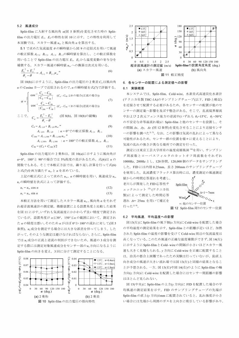
5.2 風速成分
Split-film に入射する風向角 α(図 5 参照)を変化させた時の Split-
film の出力電圧 E1,E2の特性を図 10 に示す。この特性を利用して
本実験では,スカラー風速 uscと風向角 αを算出する。
5.1 で求めた気流温度 θの瞬時値から図 9 の近似式を用いて風速
の較正係数 A(+),B(+),A(-),B(-)の瞬時値を算出し,この較正係数を
用いることで Split-film の出力電圧 E1,E2から温度変動の寄与分を
補償する。スカラー風速の瞬時値 uscへの換算は次式を用いる。
msc
s
uBAEE)()(
22
21
++ +=−+θθ
(6)
図 10(b)に示すように,Split-film の出力電圧の 2 乗差 Cαは風向角
αの Cosine カーブで近似されるので,αの瞬時値を式(7)で評価する。
ここで, θθα −
−=
s
EEC2
22
1 (図 8(b),図 10(b)の縦軸) (8)
C0 = A(-),0 + B(-),0 usc m (9) A(-),0,B(-),0 :α = 0°での較正係数 A(-),B(-)
C180 = A(-),180 + B(-),180 usc m (10) A(-),180,B(-),180 :α = 180°での較正係数 A(-),B(-)
C90 = (C0 + C180 )/2 (11) Split-film の出力電圧の 2 乗和は,図 10(a)に示すように風向角が
α=0°,180°と 90°の場合では 5%程度の差があるため,式(6)は α の
関数でもある。そこで本較正方法では,繰り返し計算を行って式(6)
と式(7)を両方満たす uscと αを求めている。
上記の較正式によって求めた usc,αの瞬時値を用い,風速成分 ux,
uyの瞬時値を次式によって評価する。
ux = usc cos α (12)
uy = usc sin α (13) 本較正方法を用いて測定したスカラー風速 usc ,風向角 αをそれぞ
れ超音波風速計の測定値,微動装置による設置角度と比較した結果
を図 11 に示す。いずれも気流温度にかかわらず良い精度で測定され
ているが,設置角度が α≦30°,150°≦αの範囲において,測定され
た αの精度は悪い。そのため αがほぼ 0°か 180°の流れに対して(図 5
参照),uy成分を測定する場合には大きな誤差を伴ってしまう。した
がって,そのような測定は避けなければならない。さらに,Split-film
では uy成分の正流と逆流の判別ができないため,風速の 3 成分を測
定する際には測定対象風速成分をセンサー部の ux方向になるように
Split-film の向きを変え,3 回に分けて測定することになる。
(a) 2 乗和 (b) 2 乗差
図 10 Split-film の出力電圧の指向特性
(a) スカラー風速 (b) 風向角
図 11 較正精度 6.各センサーの配置による測定値への影響
6.1 実験概要
本システムでは,Split-film,Cold-wire,水素炎式高速炭化水素計
(テクニカ社製 THC-1A)のサンプリングチューブ(以下,FID と略記)
を近接させて配置する必要があるため,各センサーの配置が他のセ
ンサーの測定量へ影響を及ぼす懸念がある。そこで,乱流境界層流
中および 2 次元フェンス後方の逆流中(いずれも θδ=15°C,θf =50°C
の不安定な非等温流れ場)に Split-film と他のセンサーを設置し,そ
の間隔 ∆x,∆y,∆z (図 12 参照)を変化させることにより近接センサ
ーの影響を調べた注 3)。なお,この影響は気流の乱れによって異なる
可能性があるため,センサー群の位置を様々に変えることにより,
気流の乱れの強さが異なる場所での測定を行った。
測定には東京工芸大学所有の温度成層風洞 14)を用い,サンプリン
グ周波数とローパスフィルタのカットオフ周波数をそれぞれ
1000Hz,200Hz とし,120 秒間,120,000 個のデータをサンプリング
した。FID には内径 0.25mm,長さ 200mm のサンプリングチューブ
を使用した。乱流濃度フラックス算出時には,濃度測定の風速測定
値からの時間応答遅れを考慮し,
老川らが開発した FID 応答性チ
ェックユニット 15) (テクニカ社
製)によって測定した時間応答
遅れ ∆t= 25ms を用いて補正を
行った注 4)。
6.2 平均風速,平均温度への影響
図 13(左)に Split-filmの風下側(x方向)に Cold-wireを配置した場合
の平均温度の測定結果を示す。Split-film との距離が近いほど,加熱
された Split-film の温度の影響を受けて Cold-wire 周辺の気流温度は
高くなっている。このため風速の正確な温度補償ができず,図 14(左)
に示すように Split-filmと Cold- wireの間隔が小さいほどスカラー風
速も大きく見積もられる。y 方向に Cold-wire を正確に配置すること
は,治具の都合上困難であったため実験は行っていないが,鉛直上
向き成分の風速が大きい流れ場では図 13(左)と同様の結果となるこ
とが予想される。一方,図 13(右)や図 14(右)のように Split-film の軸
方向(z 方向)に Cold-wire を配置した場合にはセンサー間距離の影響
はほとんど見られない。
図 15(中央)に Split-film の上方(y 方向)に FID を配置した場合の平
均風速の測定結果を示す。FID のサンプリングチューブの先端が
Split-film の直上(y 方向)1mm に配置されていると,乱れ強度が小さ
い場合には先端から周囲のガスを上向きに吸引している影響があり,
⎩ −−−
||cos
90180
901
CCCCα⎪
⎪⎪⎨=α
−−−
||cos
900
901
CCCCα
0
0.01
0.02
0.03
0.04
0 30 60 90 120 150 180
(<E 1
>2 -<E
2>2 )
/(θs-
<θ>)
(V2 /o C)
α (deg.)
13℃,U=0.4m/s13℃,U=1.0m/s13℃,U=1.8m/s
0.04
0.05
0.06
0.07
0.08
0 30 60 90 120 150 180
(<E 1
>2 +<E
2>2 )
/(θs-
<θ>)
(V2 /o C)
α (deg.)
uuu
0
0.5
1
1.5
2
2.5
0 0.5 1 1.5 2 2.5
<usc
>(m
/s)
超音波風速計の測定値 (m/s)
13℃30℃50℃
0
30
60
90
120
150
180
0 30 60 90 120 150 180
α(d
eg.)
Split-filmの設置角度角度 (deg.)
13℃30℃50℃
図 12 Split-film 周りのセンサー位置
y
z
x
Wind
: 他のセンサー位置
∆=1~7mm
Split film
(Ca - C90 ≧0 の場合(正流の場合))
(Ca - C90 <0 の場合(逆流の場合))
(7)

風速が僅かに大きくなっている。一方,FID が Split-film の x 方向(図
15(左))や z 方向(図 15(右))に配置される場合には,センサー間距離
の影響はほとんどない。
6.3 乱流熱フラックス,乱流濃度フラックスへの影響
図 16 では,Cold-wire を周方向(x 方向)に配置した場合と軸方向(z
方向)に配置した場合の乱流熱フラックス<u’θ’>を比較する。<u’θ’>
においても,平均温度と平均風速の場合と同様に,Cold-wire が軸方
向(z 方向,図 16(右))に配置された場合に比べ,風下側(x 方向,図
16(左))に配置された場合では,<u’θ’>はセンサー間隔 ∆x の影響を大
きく受けている。図 17(右)のように FID が軸方向(z 方向)に配置され
た場合に比べ,FID が上方(y 方向)や風下側(x 方向)に配置された場
合(図 17(左, 中央))では,乱流濃度フラックス<u’c’>が低下し,その
変化量∂<u’c’>/∂y,∂<u’c’>/∂x も大きい。このように<u’θ’>や<u’c’>
の測定値に関しても,Split-film の周方向(x,y 方向)よりも軸方向(z
方向)に他のセンサーを配置した方が,センサー間距離が測定値に与
える不確かさが小さいことが確認できる。
これらの結果と 6.2 の結果を踏まえ,風向に関わらず Cold-wire
が Split-film の風下側に位置することを避けるため,Cold-wire は
Split-film の周方向(x,y 方向)ではなく,軸方向(z 方向)にできるだけ
近接させて配置することとした。また,FID も同様に Split-film の軸
方向(z 方向)に配置することとした。
以上のように乱流熱フラックス<u’θ’>や乱流濃度フラックス
<u’c’>の測定にはセンサー位置の違いによる不確かさが存在する。
そこで,以下ではその不確かさを評価するための感度係数注 1)
∂<u’θ’>/∂z,∂<u’c’>/∂z について検討する。各無次元乱流フラックス
のセンサー間距離に対する変化量の絶対値|∂(<u’θ’>/uδ/|θδ-θf|)/∂z|,
|∂(<u’c’>/uδc0)/∂z|を乱流強度 Iu で整理すると,乱流強度の大きさや
逆流の有無に関わらず,図 18のように 1次式で近似できる。そこで,
本研究では,センサー間の距離が異なることによる<u’θ’>,<u’c’>
の 不 確 か さ を , 図 18 の 近 似 式 か ら 算 出 し た 感 度 係 数
∂(<u’θ’>/uδ/|θδ-θf|)/∂z,∂(<u’c’>/uδc0)/∂z を用いて評価した。
図 13 Split-film と Cold-wire の配置が測定温度に与える影響 図 16 Split-film と Cold-wire の配置が乱流熱フラックスに与える影響
図 14 Split-film と Cold-wire の配置が測定風速に与える影響 図 17 Split-film と FID の配置が乱流濃度フラックスに与える影響
(a) 乱流熱フラックス (b) 乱流濃度フラックス
図 15 Split-film と FID の配置が測定風速に与える影響 図 18 感度係数
-1
-0.8
-0.6
-0.4
-0.2
0
0 1 2 3
(<θ>
-θf)
/|θδ-θ f
|
∆z (mm)
-1
-0.8
-0.6
-0.4
-0.2
0
0 1 2 3
(<θ>
-θ f
)/|θ δ-θ f
|
∆x (mm)
Iu=3% Iu=10% Iu=17%Iu=110% Iu=179% Iu=334%
乱流境界層流中
2次元フェンス後方
-0.4
0
0.4
0.8
1.2
1.6
0 1 2 3
<u'θ
'>/u
δ|θδ-θ f
|
∆x (mm)
-0.4
0
0.4
0.8
1.2
1.6
0 1 2 3
<u'θ
'>/u
δ|θδ-θ f
|
∆z (mm)
x10-2x10⁻²
Iu=3% Iu=10% Iu=17%Iu=110% Iu=179% Iu=334%
乱流境界層流中
2次元フェンス後方
0
0.2
0.4
0.6
0.8
1
1.2
0 1 2 3
<usc
>/u δ
∆x (mm)
0
0.2
0.4
0.6
0.8
1
1.2
0 1 2 3
<usc
>/u δ
∆z (mm)
Iu=3% Iu=10% Iu=17%Iu=110% Iu=179% Iu=334%
乱流境界層流中
2次元フェンス後方
-0.4
-0.2
0
0.2
0.4
0 1 2 3∆z (mm)
-0.4
-0.2
0
0.2
0.4
0 1 2 3∆y (mm)
-0.4
-0.2
0
0.2
0.4
0 1 2 3
<u'c
'>/u
δc0
∆x (mm)
Iu=2% Iu=13% Iu=95%Iu=200% Iu=441% Iu=489%
乱流境界層流中
2次元フェンス後方
0
0.2
0.4
0.6
0.8
1
1.2
0 1 2 3
<usc
>/u δ
∆x (mm)
0
0.2
0.4
0.6
0.8
1
1.2
0 1 2 3∆z (mm)
0
0.2
0.4
0.6
0.8
1
1.2
0 1 2 3∆y (mm)
Iu=2% Iu=13% Iu=95%Iu=200% Iu=441% Iu=489%
乱流境界層流中
2次元フェンス後方
0
0.5
1
1.5
2
2.5
3
0% 200% 400% 600%
感度
係数
(1/m
m)
Iu (%)
乱流境界層流中
2次元フェンス後方0
0.2
0.4
0.6
0.8
1
1.2
0% 200% 400% 600%
感度
係数
(1/m
m)
Iu (%)
乱流境界層流中
2次元フェンス後方
x10-3 x10⁻²
R2= 0.943
R2= 0.961

7.逆流域を含む流れ場の測定例
7.1 実験概要
本測定システムと前述した熱線と冷線の較正装置および較正式を
用いて,2 次元フェンス後方の逆流を含む流れ場を測定した結果に
ついて述べる。対象とした流れ場を図 19 に示す。2 次元フェンスに
は高さ 80mm,厚さ 5mm のアルミ製の板を使用し,風洞気流に対し
て直角に配置した。トレーサーガス(C2H4)は 2 次元フェンスの風下
側 120mm (X/H=1.5)の位置に設けた φ5mm の孔から流量 q=9.17x10⁻⁶
m3/s で放出した。実験には東京工芸大学の温度成層風洞を用い,流
れ場の条件を等温(Rb=0)と安定な非等温状態(Rb=0.11),不安定な非
等温状態(Rb= -0.14)の 3 ケース(表 1)に設定した。本測定では,風速
の u 成分を測定する際には,Split-film の方向を ux=u とし,w 成分の
測定時には ux=w となるようにセットした(ux成分は図 5 参照)。サン
プリング周波数 1000Hz で 120 秒間の測定を行った。ローパスフィ
ルタによるカットオフ周波数は 200Hz とした。
図 19 対象とする流れ場
表 1 風洞の気流条件
Case Rb=0.11 Rb=0 Rb= -0.14 Rb 0.11 0 -0.14Re 1.2x10⁴ 1.2x10⁴ 1.2x10⁴
uH(m/s) 1.1 1.1 1.1θf (oC) 18.0 16.8 48.1θH(oC) 45.0 16.5 16.6θ0 (oC) 40.3 16.8 20.9θgas (oC) 31.0 16.8 31.1
Bulk Richardson number: Rb = gH(θH-θf) /{(θ0 +273)(uH 2)}
7.2 測定結果
(1) センサーによる不確かさの違い
本測定手法を用いて,弱安定成層条件下(Rb=0.11)で測定したフェ
ンス後方 X/H=1.0 での平均スカラー風速の鉛直分布を図 20(a)に示
す。図 20(a)には,I-wire で測定した結果注 5)も併せて示すが,その
結果は Split-film の不確かさ範囲内に収まっており,よく一致して
いる。
図 20(b)では,平均スカラー風速<usc>に対する拡張不確かさ注 1)
Ue(<usc>/uH)を示し,グラフ中の点線の傾きによって相対不確かさ
Ue(<usc>/uH)/|<usc>/uH|を百分率で表す。フェンスより高い強風域
(<usc>/uH≧0.3)では,I-wire で測定した平均スカラー風速の拡張不確
かさは,多くの測点で相対不確かさ 5%のラインを下回っているの
に対し,Split-film による測定値の相対不確かさは 11%~13%であっ
た。フェンス後方弱風域(<usc>/uH≦0.3)では,I-wire,Split-film とも
に測定値の相対不確かさは若干大きくなっているが,図 20(a)に示す
ようにその拡張不確かさの絶対値は小さい。
(a) <usc>の鉛直分布 (b) <usc>の拡張不確かさと相対不確かさ
図 20 Split-film と I-wire の実験結果の比較 (X/H=1.0) (2) 本測定手法の不確かさ評価
1) 平均風速
2 次元フェンスの風下側 X/H=1.0 での平均風速<u>の鉛直分布を
図 21(a)に示し,図 21(b)には平均風速<u>の拡張不確かさ Ue(<u>)
を示す。等温条件(Rb=0.00)では孟らによって提案された較正手法 16)
を用い,非等温条件では本較正手法を用いた。その拡張不確かさは
等温条件である Rb=0.00 のケースで最も小さく,Rb=-0.14,Rb=0.11
の順で大きくなっている。このように非等温条件では温度測定に起
因する不確かさ要因があるため,等温条件よりもその拡張不確かさ
が概ね 4%程度大きくなっている。
(a) 鉛直分布 (b) 拡張不確かさと相対不確かさ 図 21 平均風速<u>の分布 (X/H=1.0)
2) 平均温度と乱流熱フラックス
図 22(b)に示した平均温度<θ>の拡張不確かさは概ね 5%のライン
を下回っており,その拡張不確かさ範囲は図 22(a)でも判別できない
ほど小さいため,測定値の信頼性は高い。図 23(b)に示した乱流熱フ
ラックス<u’θ’>の相対拡張不確かさは,どちらの非等温条件でも
20%を超え,測定値が小さい場合には 100%のラインを上回る測定点
もある。この原因としては,図 23(a)に示すように乱流熱フラックス
の値が非常に小さくゼロに近いため,拡張不確かさの絶対値が小さ
い場合でも,相対的な値は大きくなることが挙げられる。また,フ
ェンス後方弱風域では測定の繰り返し性注 6)とセンサー間距離によ
る要因が大きく,測定の繰り返し性とセンサー間距離の標準不確か
さが拡張不確かさに占める割合は,それぞれ 1~2 割と 2~4 割程度
であった。
3) 平均濃度と乱流濃度フラックス
図 24(b)に示した平均濃度<c>の拡張不確かさは,ほぼ 20%のライ
ンを下回っているが,平均風速や平均温度の測定結果に比べると大
きく,ばらつきがある。これは濃度変動の間欠性が大きく,測定の
繰り返し性による実験標準偏差 s 注 1)が大きかったためである。この
影響から,図 25(b)の乱流濃度フラックス<u’c’>の拡張不確かさに占
X/H=1.5 ガス排出孔(φ5mm)
C2H4
H=0
.08m
測線X/H=1.0
0
0.5
1
1.5
2
0 0.5 1 1.5
Z / H
<u>/ uH
Rb= 0.11Rb= 0.00Rb=-0.14
0
0.05
0.1
0.15
0.2
0 0.5 1 1.5 2
拡張
不確
かさ
Ue(<
u sc>
/uH
)
測定値 <usc> /uH
Split-filmI-wire
00.5
11.5
22.5
33.5
4
0 0.5 1 1.5 2
Z/H
<usc> /uH
Split-filmI-wire
:不確かさ範囲
0
0.05
0.1
0.15
0.2
-0.5 0 0.5 1 1.5 2
拡張
不確
かさ
Ue(<
u> /u
H)
測定値 <u> /uH
00.5
11.5
22.5
33.5
4
-0.5 0 0.5 1 1.5 2
Z/H
<u> /uH
:不確かさ範囲
Rb= 0.11Rb= 0.00Rb=-0.14
Rb= 0.11Rb= 0.00Rb=-0.14

める濃度変動の繰り返し性注 6)の標準不確かさの割合も 6 割以上と
大きく,<u’c’>の相対不確かさはほぼ全点で 50%を超えている。こ
の不確かさは試行回数を増やすことによって低減可能である。その
例として,図 25 中のある 1 点(Z/H=0.3125)において,試行回数 n を
2~9 回と変化させたときの<u’c’>の相対不確かさの変化を図 26 に
示す。図 25 は n=3 回の試行回数に基づく結果であるが,図 26 によ
れば試行回数を 3 回から 6 回に増やすことでその相対不確かさを半
分程度にまで減らすことができる。今後の CFD 検証用風洞実験の際
には数回以上の試行回数が望ましいことが明らかとなった。
(a) 鉛直分布 (b) 拡張不確かさと相対不確かさ 図 22 平均温度<θ>の分布 (X/H=1.0)
(a) 鉛直分布 (b) 拡張不確かさと相対不確かさ 図 23 乱流熱フラックス<u’θ’>の分布 (X/H=1.0)
(a) 鉛直分布 (b) 拡張不確かさと相対不確かさ 図 24 平均濃度<c>の分布 (X/H=1.0)
(a) 鉛直分布 (b) 拡張不確かさと相対不確かさ 図 25 乱流濃度フラックス<u’c’>の分布 (X/H=1.0)
図 26 試行回数による乱流濃度フラックスの相対不確かさの変化
(Rb=0.00,X/H=1.0, Z/H=0.3125)
8.まとめ
本研究では,非等温流れ場における建物周辺気流の風速,温度,
濃度の同時測定を目的とし,それを実現する測定システムを開発し,
較正方法を提案した。以下に本研究で得られた知見をまとめる。
1) 製作した熱線と冷線の較正装置内の風速と温度の乱れ強度 Iu,Iθは,較正風速 uc=0.2~3.55m/s の範囲においてそれぞれ Iu<1%,
Iθ<2%であり,安定した風速と温度の供給を可能にしている。
2) Split-film の周囲に Cold-wire や FID のサンプリングチューブを
近接配置して測定値への影響を調査した結果,Split-film の軸方
向に他のセンサーを配置した場合に影響が最も少ないことが明
らかとなった。
3) 提案した Split-film の較正式によって,逆流を伴う非等温流れ場
での風速と温度の同時測定が可能となった。測定された平均風
速の相対不確かさは強風域で 10%~13%である。弱風域では,
相対不確かさが 20%以上と強風域よりも大きいが,その拡張不
確かさの絶対値は小さい。その他の平均量の相対不確かさは,
平均温度で 5%以下,平均濃度で 3%~20%である。
4) 風速,温度,濃度の同時測定によって得られた乱流熱フラック
ス,乱流濃度フラックスの相対不確かさはそれぞれ,20%以上,
50%以上である。しかし,いずれの測定量の拡張不確かさにお
いても,測定の繰り返し性の影響が大きく,測定の試行回数を
増やすことで改善することができる。
9.おわりに
現在,この測定手法を用いて建物背後や都市街区内のような非等
温弱風域の風洞実験を行い 17),18),19),CFD 検証用の実験データベース
を作成し,汚染物質や熱の移流・乱流拡散による輸送構造について
調査している。さらに今後は,建築学会の「屋外空気環境予測・評
価小委員会」の活動の一環として,これらの風洞実験を対象とした
非等温弱風流れ場の CFD ベンチマークテストを行い,ヒートアイラ
ンド現象や大気汚染の問題に CFD を適用する際の精度と問題点を
明らかにしていく予定である。
謝辞
本研究の一部は東京工芸大学 21 世紀 COE プログラムによる成果
である。また,本論文の投稿にあたっては,匿名の査読者から大変
有意義なご助言を頂いた。ここに記して謝意を表す。
注
注 1) 測定結果に信頼性を付加するために用いる不確かさとは,「測定の結果
に付随した,合理的に測定量に結び付けられ得る値のばらつきを特徴づ
0
0.025
0.05
0.075
0.1
0 0.5 1 1.5 2測定値 <θ>/|θH-θf|
00.5
11.5
22.5
33.5
4
0 0.5 1 1.5 2 2.5
Z/H
<θ> /|θH-θf|
:
不確かさ範囲
拡張
不確か
さU
e(<θ>
/|θH-θ f
|)Rb= 0.11Rb=-0.14 Rb= 0.11
Rb=-0.14
0
0.001
0.002
0.003
0.004
0.005
0 0.0025 0.005 0.0075 0.01測定値 |<u'θ'> /uH/|θH-θf||
00.5
11.5
22.5
33.5
4
-0.01 -0.005 0 0.005
Z/H
<u'θ'> /uH|θH-θf|
:
不確かさ範囲
拡張
不確
かさ
Ue(|
<u'θ
'> /u
H/|θ
H-θ f
||)Rb= 0.11Rb=-0.14 Rb= 0.11
Rb=-0.14
0
1
2
3
4
5
6
0 20 40 60
拡張
不確かさ
Ue(<
c> /c
0)
測定値 <c> /c0
00.5
11.5
22.5
33.5
4
0 20 40 60
Z/H
<c> /c0
:不確かさ範囲
Rb= 0.11Rb= 0.00Rb=-0.14
Rb= 0.11Rb= 0.00Rb=-0.14
0
0.5
1
1.5
2
2.5
3
0 1 2 3測定値 |<u'c'> /uHc0|
00.5
11.5
22.5
33.5
4
-4 -3 -2 -1 0 1
Z/H
<u'c'> /uHc0
:不確かさ範囲
Rb= 0.11Rb= 0.00Rb=-0.14
Rb= 0.11Rb= 0.00Rb=-0.14
拡張
不確
かさ
Ue(|
<u'c
'> /u
Hc 0
|)
0
30
60
90
120
0 1 2 3 4 5 6 7 8 9 10
相対
不確かさ(
%)
試行回数 n

けるパラメータ」として定義されている 13)。これは,「測定値は真値では
なく,最良推定値である」という前提に基づいており,その評価方法は参
考文献 13), 20)を要約すると以下のように示される。
ある測定量 Xm1, Xm2, . . , XmNの推定値 ξ1, ξ2, . . , ξN によって決定される
推定値 ζが式(14)で表されるとする。
ζ = f (ξ1, ξ2, . . , ξN ) (14)
この推定値 ζ の合成標準不確かさ Uc(ζ) は,各推定値 ξi の標準不確かさ
U(ξi)を合成して式(15)によって算出される。もし各測定量間に相関があ
る場合は,推定共分散 U(ξi, ξj)を用いて式(16)によって合成標準不確かさ
Uc(ζ)が計算される。なお,式(15),(16)中の∂f /∂ξiは感度係数と呼ばれる。
Uc (ζ) = 2
1
)(∑= ⎭
⎬⎫
⎩⎨⎧∂∂N
ii
i
Uf ξξ
(15)
Uc (ζ) = ),(2)(1
1 1
2
1j
N
i
N
iji
ji
N
ii
i
UffUf ξξξξ
ξξ ∑ ∑∑
−
= +== ∂∂
∂∂
+⎭⎬⎫
⎩⎨⎧∂∂
(16)
この標準不確かさ U(ξi)は評価方法の違いによって Type A と Type B の評
価方法に分類される。Type A は統計的手法による評価であり,式(17)に
よって標準不確かさ U(ξi)が算出される。ここで,s(ξi)は推定値 ξi の実験
標準偏差であり,n は自由度である。代表的な例として,繰り返し測定
された平均値 ξiの標準偏差が s(ξi),繰り返し回数が n に相当する。Type B
は統計的手法以外の評価方法であり,測定機器メーカーの仕様や較正証
明書など適切な情報に基づいた工学的判断によって評価される。
U (ξi) = n
s i )(2 ξ (17) 本実験では,包含係数K を 95%の信頼の水準に基づいて算出している。
この包含係数 K を使用して式(18)によって拡張不確かさ Ue(ζ)を求め,式
(19)によって測定量 Zmを表す。
Ue(ζ) = K Uc(ζ) (18)
Zm = ζ ± Ue(ζ) (19)
また,ζの相対不確かさは Ue(ζ)/|ζ| の百分率で表わされる。
注 2) 較正風速範囲よりもさらに低風速の範囲(-0.5m/s~0.5m/s)について
は,風洞実験時に測定した気流温度 θ における E1,E2と uscの関係から
スプライン関数を用いて内挿補間している。
注 3) 各センサーはマイクロメータ(測定精度:±0.05mm)を組み込んだ治具に
よって風洞の微動装置に取り付けられており,このマイクロメータによ
って各センサー間距離の調整を行っている。
注 4) FID 応答性チェックユニット 15)により測定した時間応答遅れ ∆t=25ms
は,サンプルガスがサンプリングチューブ先端から FID 燃焼室に達する
時間 t1と FID 燃焼室に達してから出力が一定値の 63.2%に到達するまで
の時間 t2 の和である。それらの解析値は,テクニカ社が示している解析
手法 21),22)等によると,それぞれ t1=15.4ms,t2=9.8ms,∆t =t1+t2=25.2ms と
なり,FID 応答性チェックユニットによる時間応答遅れの測定値とほぼ
一致している。風洞実験では,この ∆t=25ms を用い,測定した風速の瞬
時値 u(t)よりも 0.025 秒後の濃度の瞬時値 c(t+0.025)を同じタイミングの
測定値として乱流濃度フラックス u’c’(t)を算出している。
注 5) I-wire の較正は,式(2),(3),(6)中の E12+E2
2を I-wire の出力電圧 E の
2 乗 E2に置き換えて行った。
注 6) 測定の繰り返し性による標準不確かさ U (ξi)は,繰り返し測定の結果得
られた時間平均値を式(17)より算出している。風速 3 成分の測定では 40
秒間を 3 回(計 120 秒)行い,風速に関連した測定量(平均風速,レイノル
ズ応力,乱流フラックス)では 3 回の試行回数を有している。また,温度
と濃度に関連した測定量(平均値,標準偏差)では,同一測定点で風速の 3
成分ごとに温度と濃度を同時に測定しているため,計 9 回の試行回数を
有する。
参考文献 1) 日本建築学会:市街地風環境予測のための流体数値解析ガイドブック -ガ
イドラインと検証データベース-, 2007 2) 村上周三, 大岡龍三, 足永靖信, 河野孝昭, 大黒雅之, 谷本潤, 持田灯, 松縄
堅: ヒートアイランド現象緩和に関する評価システム構築のための CFDによる感度解析, 日本建築学会技術報告集, No.23, pp.241-246, 2006.6
3) 足永靖信, 東海林孝幸, 河野孝昭: 地球シミュレータを用いた東京都心
10km 四方における高解像度のヒートアイランド数値解析, 日本建築学会
環境系論文集, No.616, pp.67-72, 2007.6 4) 加藤信介, H.Huang, 大岡龍三, T.Jiang: CFD 解析による市街地における
Visitation frequency, Purging flow rate の解析 高架道路周辺換気効率の評
価に関する研究, 風工学シンポジウム論文集, Vol.15, pp.93-98, 2004.11 5) A.Mochida, Y.Tominaga, S.Murakami, R.Yoshie, T.Ishihara and R.Ooka:
Comparison of various k-ε models and DSM to flow around a high rise building - report of AIJ cooperative project for CFD prediction of wind en-vironment, Wind & Structures, Vol. 5, No. 2-4, pp.227-244. 2002.3
6) 白澤多一, 富永禎秀, 義江龍一郎, 持田灯, 吉野博, 片岡浩人, 野津剛: CFDを利用した高層建物周辺の風環境評価手法の開発(その 2) 4:4:1 角柱モデ
ルを対象とした各種改良 k-εモデルの相互比較, 日本建築学会技術報告集, No.18, pp.169-174, 2003.12
7) 富永禎秀, 持田灯, 張本和芳, 片岡浩人, 義江龍一郎: CFD を利用した高層
建物周辺の風環境予測(その 3) 実在市街地モデルを対象としたベンチマ
ークテスト, 日本建築学会技術報告集, No.19, pp.181-184, 2004.6 8) R.Yoshie, A.Mochida, Y.Tominaga, H.Kataoka, K.Harimotoe, T.Nozu,
T.Shirasawa: Cooperative project for CFD prediction of pedestrian wind en-vironment in the Architectural Institute of Japan, Journal of Wind Engineering and Industrial Aerodynamics, Vol.95, pp.1551-1578, 2007.2
9) 上原清, 村上周三, 老川進, 若林伸司: 温度成層流中のストリートキャニオ
ン内の流れに関する LDV を用いた風洞実験, 日本建築学会計画系論文集, No.492, pp.39-46, 1997.2
10) Y.Ogawa, P.G.Diosey, K.Uehara, H.Ueda: Plume behavior in stratified flows, Atmospheric Environment, Vol.16, No.6, pp.1419-1433, 1982
11) Y.Ohya: Wind tunnel study of atmospheric stable boundary layers over a rough surface, Boundary-Layer Meteorology,Vol.98, pp.57-82, 2001.1
12) R.Zegadi, M.Ayarault, P.Mejean: Effect of a two-dimensional low hill in a thermally neutral and stable stratified turbulent boundary layer, Atmospheric Environment, Vol.28, No.11, pp.1871-1878, 1994
13) 日本規格協会: 計測における不確かさの表現のガイド, 1996 14) 大場正昭, 栗田剛, 名和健太郎: 室内回流式エッフェル型温度成層風洞の
紹介, 日本風工学会誌, No.88, pp.73-80, 2001.7 15) 老川進, 孟 岩: 建物後流における短時間ピーク濃度の性状について, 大気
環境学会誌, No.33, pp.151-163, 1998.5 16) 孟 岩, 日比一喜: 高層建物屋上の流れ場の乱流特性と組織運動, 日本風工
学会誌, No.72, pp.21-34, 1997.2 17) 小林剛, 義江龍一郎, 田中英之, 白澤多一: 弱風域を対象とした流れ場・温
度場・拡散場に関する風洞実験と数値解析(その 1) 非等温流れ場の風
速・温度・濃度の同時測定手法と平均量の測定結果, 日本建築学会大会学
術講演梗概集(D2), pp.695-696, 2007.8 18) 田中英之, 義江龍一郎, 小林剛, 白澤多一: 弱風域を対象とした流れ場・温
度場・拡散場に関する風洞実験と数値解析(その 2) 非等温流れ場におけ
る熱フラックス・濃度フラックス等の乱流統計量, 日本建築学会大会学術
講演梗概集(D2), pp.697-698, 2007.8 19) 義江龍一郎, 田中英之, 白澤多一, 小林剛: 香港の高層密集市街地における
風通しに関する研究(その 1) 建蔽率と建物高さのバリエーション等が歩
行者レベルの風速・気温分布に及ぼす影響, 日本建築学会大会学術講演概
要集(D1), pp.745-746, 2007.8 20) L.Kirkup, R.B. Frenkel: An introduction to uncertainty in measurement, 2006 21) J.Lawton, F.J.Weinberg: Electrical aspects of combustion, Clareudon Press,
1969 22) J.M.Goodings: Detailed ion chemistry in methane-oxygen flames-negative
ions, Combustion and Flame, Vol.36, pp.45, 1979