ailawadi, k. l., & neslin, s. a. (1998). the effect of promotion on consumption- buying more and...

The Effect of Promotion on Consumption: Buying More and Consuming It FasterAuthor(s): Kusum L. Ailawadi and Scott A. NeslinSource: Journal of Marketing Research, Vol. 35, No. 3 (Aug., 1998), pp. 390-398Published by: American Marketing AssociationStable URL: http://www.jstor.org/stable/3152036 .

Accessed: 01/10/2013 04:42

Your use of the JSTOR archive indicates your acceptance of the Terms & Conditions of Use, available at .http://www.jstor.org/page/info/about/policies/terms.jsp

.JSTOR is a not-for-profit service that helps scholars, researchers, and students discover, use, and build upon a wide range ofcontent in a trusted digital archive. We use information technology and tools to increase productivity and facilitate new formsof scholarship. For more information about JSTOR, please contact [email protected].

.

American Marketing Association is collaborating with JSTOR to digitize, preserve and extend access toJournal of Marketing Research.

http://www.jstor.org

This content downloaded from 130.115.84.35 on Tue, 1 Oct 2013 04:42:39 AMAll use subject to JSTOR Terms and Conditions

http://www.jstor.org/action/showPublisher?publisherCode=ama

http://www.jstor.org/stable/3152036?origin=JSTOR-pdf

http://www.jstor.org/page/info/about/policies/terms.jsp


KUSUM L. AILAWADI and SCOTT A. NESLIN*

The authors empirically demonstrate the existence of flexible consumption rates in packaged-goods products, how this phenomenon can be modeled, and its importance in assessing the effectiveness of sales promotion. They specify an incidence, choice, and quantity model in which category consumption varies with the level of household inventory. The authors use two different functions to relate consumption rates to household inventory and estimate the models using scanner panel data from two product categories: yogurt and ketchup. Both functions provide a significantly better fit than a conventional model, which assumes a constant daily usage rate. They also have strong discriminant validity; yogurt consumption is found to be much more flexible with respect to inventory than ketchup consumption is. The authors use a Monte Carlo simulation to decompose the long-term impact of promotion into brand switching and consumption effects and conclude with the implications of their findings

for researchers and managers.

The Effect of Promotion on Consumption:

Buying More and Consuming It Faster

Researchers have spent more than a decade using scanner data to investigate the effect of sales promotion. They have established that promotion results in a significant temporal and cross-sectional shifting of category demand (e.g., Blat- tberg and Wisniewski 1989; Gupta 1988). Conspicuously, however, there is little empirical research that measures promotion's potential to increase category demand (for excep- tions, see Chandon and Laurent 1996; Chiang 1995; Dillon and Gupta 1996), though both academics and managers appear to be well aware of the potential for such an effect (cf. Blattberg and Neslin 1990, pp. 133-35).

Promotion's effect on consumption stems from its funda- mental ability to increase household inventory levels. High- er inventory, in turn, can increase consumption through two mechanisms: fewer stockouts and an increase in the consumer's usage rate of the category. The first of these is simple-fewer stockouts mean the household has more oppor-

*Kusum L. Ailawadi is an associate professor and Scott A. Neslin is Benjamin Ames Kimball Professor of the Science of Administration, Amos Tuck School of Business Administration, Dartmouth College (e-mail: [email protected] and [email protected]). Authors' names are listed in alphabetical order to reflect their equal contri- bution. The authors appreciate comments from Randy Bucklin, Jeongwen Chiang, Pradeep Chintagunta, Paul Farris, Karen Gedenk, Sachin Gupta, Jeff Inman, John Little, Purushottam Papatla, Bob Shoemaker, Steve Shugan, Kannan Srinivasan, Brian Wansink, and participants in the 1995 Northwestern Research Seminar, 1996 INFORMS Marketing Science Con- ference, and 1996 Association for Consumer Research Conference. They are also grateful to John Harris and John Roback for computing support. This research was supported by the Tuck Associates Program.

Journal of Marketing Research Vol. XXXV (August 1998), 390-398

tunities to consume the product. Existing models of purchase incidence and quantity can capture this mechanism because they allow promotion-induced purchasing to increase inventory and therefore reduce stockouts (e.g., Buck- lin and Lattin 1991; Chintagunta 1993; Guadagni and Little 1987; Gupta 1988, 1991). Neslin and Stone (1996, p. 89), in a study on purchase acceleration, note that promotion also increases consumption "due to higher inventory levels, and hence fewer stockouts under the promotion scenario."

The second mechanism, which says that households increase their usage rate when they have high inventory, is supported by both economic and behavioral theory. As- suniao and Meyer (1993) show that consumption should increase with inventory, not only because of the stock pressure from inventory holding costs, but also because higher in- ventories give consumers greater flexibility in consuming the product without having to worry about replacing it at high prices. Scarcity theory suggests that consumers curb consumption of products when supply is limited because they perceive smaller quantities as more valuable (e.g., Folkes, Martin, and Gupta 1993). Wansink and Deshpand6 (1994) show that increased inventory generated by promotion can result in a faster usage rate if product usage-related thoughts are salient, that is, if products are perishable, are more versatile in terms of potential usage occasions (e.g., snack foods), need refrigeration, or occupy a prominent place in the pantry.

Although these studies provide important theoretical jus- tification for the existence of a flexible usage rate, we are not aware of any attempts to model this phenomenon in

390



The Effect of Promotion on Consumption

scanner data-based models.I Most purchase incidence and quantity models assume a constant usage rate for the household (e.g., Bucklin and Lattin 1991; Chintagunta 1993; Gupta 1988, 1991; Tellis and Zufryden 1995). This omits the usage rate mechanism and potentially results in an un- derestimate of the effect of promotion on consumption.

Our goal here is to (1) demonstrate empirically the existence of the flexible usage rate phenomenon, (2) show how it can be modeled, and (3) illustrate its importance in evalu- ating the effectiveness of promotion. A function that enables usage rate to vary with the level of household inventory is embedded in a model of purchase incidence and quantity. We use two different usage rate functions to suggest alternative modeling approaches, as well as to provide convergent validity for the flexible usage rate phenomenon. We estimate the complete model using each function for two product categories, yogurt and ketchup, across which the flexibility of usage rates is expected to differ substantially. Our results establish the existence of the phenomenon and provide convergent, as well as discriminant, validity for the functions used to model it.

The article is organized as follows: The next section de- scribes our model, focusing on the flexible usage rate. We then summarize the data used for the empirical analysis and the results of our estimation, as well as the findings of a Monte Carlo simulation designed to measure the increase in consumption due to promotion. We conclude with a discussion of our key findings, their implications, and some sug- gestions for additional research.

THE MODEL

We model the purchase incidence, brand choice, and purchase quantity decisions for a household. Household inventory is an explanatory variable in the incidence and quantity decisions and is associated directly with the flexible usage rate phenomenon that is the central focus of our article. We therefore begin our model description with the inventory identity and usage rate function.

Inventory Identity Similar to other researchers, we use the following identity

to calculate household inventory recursively at the beginning of each shopping trip (e.g., Bucklin and Lattin 1991; Chintagunta 1993; Gupta 1988; Tellis and Zufryden 1995):

(1) Invh = InvhI + PurQtyh_ - Consumpth

where

Invh = inventory carried by household h at beginning of shopping trip t,

PurQtyth_ = quantity (in ounces) purchased by household h during trip t- 1, and

Consumpth_ = consumption (in ounces) by household h since trip t- 1.

Typically, the starting inventory for each household is set equal to the average weekly consumption level of the house-

IWiner (1980a, b) examines the impact of advertising on consumption using panel data from a split cable experiment. However, he assumes that households consume all their inventory of the category before their next purchase.

hold.2 Thus, the starting inventory is 7 x Ch, where Ch is the household's average daily consumption level computed from an initialization period, that is, the total volume of product purchased by household h over the duration of the initialization period, divided by the number of days in the period. Then, inventory at the beginning of each subsequent shopping trip is calculated recursively by adding the amount purchased on the previous trip and subtracting the amount consumed since the previous trip.

Usage Rate Function

Researchers have assumed a constant daily usage rate, also equal to Ch. In these models, termed the status quo hereafter, daily consumption is calculated as

(2) Consumpth = min{Invh,C },

where Consumptht is the consumption during day t by household h, and Invht is the inventory held by household h at the beginning of day t. Households are assumed to consume Ch ounces of the product per day if their available inventory is equal to or more than Ch If available inventory is less than Ch, the entire amount is consumed (e.g., Gupta 1988).3

Instead of this status quo, we allow the usage rate during a given day to vary depending on the inventory available to the household at the beginning of that day. Then, we recursively calculate inventory at the end of each day the same way other researchers do. Beginning inventory on any given day is logically and temporally prior to the consumption during that day. We use two different functional forms for the usage rate to illustrate alternative approaches for modeling the phenomenon and to provide a test of convergent validity. These functions are described next.

Flexible usage rate: A spline function. One of the sim- plest ways to think about flexible consumption is by consid- ering that households might consume their inventory at a higher rate soon after a purchase (i.e., when inventory is high) compared with later times, instead of at a single constant rate.4 This can be represented by a spline function with a single node. To retain heterogeneity in usage rates across households while limiting the number of additional parameters to be estimated, we specify the spline function so that the daily usage rate is a x Ch for a period immediately after a purchase, and Ch thereafter. Furthermore, because households may differ in their purchase frequency, we assume that the change in usage rate, that is, the node of the spline function, occurs at half the household's average interpur- chase time, Th. Finally, we impose the restriction that consumption on any given day cannot exceed the inventory available at the beginning of that day. Therefore, the spline function is as follows:

2The empirical results in this article are not sensitive to the particular starting inventory used.

3Some researchers (e.g., Chintagunta 1993) allow inventory levels to be negative. The fit of our continuous usage rate model, described subse- quently, is significantly better than both this model and the model in Equa- tion 2.

4We thank an anonymous reviewer for suggesting this approach to us.

391



JOURNAL OF MARKETING RESEARCH, AUGUST 1998

(3) Consumpth =

-h ^h

min(lnvth, aC ) if days < 2

h-h ) ida h min(InvP,Ch) if days > 2

Figure 1 EFFECT OF Ch

(f = 1.0)

where a is the parameter to be estimated, and days are the number of days since the last purchase. This function provides a parsimonious and simple way to document the phenomenon of a flexible usage rate. If usage rate does increase with inventory, we would expect a to be greater than 1, which is the value assumed in status quo models.

Flexible usage rate: A continuous nonlinear function. Al- though simple, the spline function is not particularly appeal- ing from a behavioral viewpoint. Although it makes sense for households to consume more immediately after a purchase, when inventory tends to be higher, it is difficult to understand why they would consume at one constant rate for awhile and then, at some arbitrary point, switch over to a slower but still constant rate, irrespective of how much they purchased. The switch-over point that provides the best statistical fit could be estimated from the data, but it would add another parameter and not improve the behavioral interpre- tation of the function. Instead of the spline model, it is be- haviorally more reasonable to assume that household consumption varies continuously and nonlinearly with actual inventory. This is the case with behavioral response to many physical stimuli, as is consistent with the Weber-Fechner and Power Function Laws found in psychophysical literature (Engel, Blackwell, and Miniard 1995, pp. 475-76; Stevens 1986, pp. 1-19). We therefore specify an alternative usage rate function that models daily consumption as a continuous, nonlinear function of available inventory:

(4)

-h Consumptth = Invth h

C +(Inv_h)f

This function, whose shape is depicted in Figures 1 and 2, has several additional desirable characteristics:

1. It is parsimonious with only a single parameter "f' to be estimated.

2. Consumption does not exceed available inventory, so there is no need to truncate consumption, as in the case of the spline function.

3. For a given value of f, heavy users (with high Ch) consume more than light users at any given inventory level. We illustrate this in Figure I by graphing the function at various values of Ch while keeping f fixed. The figure shows that higher Chs move the function upward without changing its shape much.

4. The value of f, which we term the flexibility parameter, de- termines how responsive consumption is to high levels of inventory.5 Figure 2 shows that, for a given value of Ch, if f is negative, households tend to consume almost all that is available to them. If f is positive, households are not as flexible in their usage rate. For f = 1, this usage rate function is similar

5Similar to most nonlinear functions, our usage rate function is not invariant with respect to the units of measurement. Therefore, its shape at various values of f should be evaluated for a range of inventory values that correspond to the data being used. Our data for yogurt and ketchup are mea- sured in ounces, and in the discussion that follows, we evaluate the usage rate function for inventory in multiple ounces.

o e.

r,

o U

8 + +4--

1- -. 4 I II II++ IIIII..I1IIII1III--- . . . . .

0rl' IIIll IIIIIll Ill II III III IIIIII IfIIIIII III IIIIIII 1 5 9 13 17 21 25 29 33 37 41 45 49

Available Inventory

Ch= I ....... Ch=5

I ~h = 10

to the status quo, in that households initially increase consumption with inventory, but when they approach their average usage rate Ch, consumption remains constant, even for high values of inventory.6

Consequently, this usage rate function is able to map out varying levels of flexibility in consumption through the parameter f. Status quo models, by not allowing consumption to vary with inventory levels greater than Ch, essentially have assumed a value of f equal to 1. We, however, empirically estimate the value of f.

Model for Brand Choice, Purchase Incidence, and Purchase Quantity

We link the choice and incidence models through a standard nested logit formulation and incidence and quantity decisions through a hurdle formulation (Mullahy 1986).7 Although the former is standard in the literature, the latter deserves some discussion. A binomial logit model governs purchase incidence, and if the "hurdle" is crossed and a purchase takes place, the conditional distribution of the number of units purchased is governed by a truncated-at-zero Pois- son model. The advantage of this hurdle formulation is that the incidence and quantity models, both of which contain the inventory variable and therefore are affected by the usage rate function, can be estimated jointly. In addition, the Poisson model, unlike regression models used in the literature, provides integer predictions of purchase quantity.

The specific formulations for brand choice, purchase incidence, and purchase quantity models are described subse- quently. The explanatory variables used in each model are based on existing literature (e.g., Bucklin and Lattin 1991;

6This also can be demonstrated analytically by calculating the first deriv- ative of the function at f = I and taking the limit as inventory goes to oo.

7We thank Pradeep Chintagunta, University of Chicago, for suggesting this approach to us.

392




Figure 2 EFFECT OF FLEXIBILITY PARAMETER f (Ch = 2)

30

25 -

_.+ ,+

4- Xx

+'+ _ x,X

.+"+0 ^Xl

..f +

Xx'

,. .x.

1+' -,Xx-"

,+X X + -- - -- - - -- - - ---- ---

+,-I-' x , X '

..I X.l-~-"._.._- - .. ..

Equation 5, namely, the inclusive value in nested logit), inventory (mean-centered for each household), Ch, and lagged purchase incidence. We include the lagged incidence variable to model systematic swings in purchase and consumption due to eating bouts, binging, special diets, and other situational factors (see, for example, Logue 1991; McAlister and Pessemier 1982; Wansink 1994). As a result of these phenomena, category purchase on one shopping trip might be associated with a higher likelihood of purchase on the next trip.9

Purchase quantity. A truncated-at-zero Poisson model governs probability of purchasing q units (q > 1), given that the purchase incidence hurdle has been passed.

(7) (Xh )q

Pth(qlinc & j) = jt

(e jt - 1)q!

o . I I I I I I I I I I I I I I I I I I I I I I I I I I I I

1 3 5 7 9 11 13 15 17 19 21 23 25 27 29

Available Inventory

....... f= 1.00

f = .5

-X-f=0

Bucklin and Silva-Risso 1996; Guadagni and Little 1983; Gupta 1988; Tellis and Zufryden 1995) and are detailed in the Appendix.

Brand choice. The probability Pht(jlinc) that a household h will choose brand size j during shopping trip t, given that the product category is being purchased, is modeled as8

Ph(jlinc) = e

XeUht ' k, kt

kcKst

where Kst is the set of brand sizes available in store s in which the household shops on the tth shopping trip, and Uhjt, the systematic utility of a given brand size, is a linear function of its shelf price per ounce (whether or not it is on promotion) and the loyalty of the household to the brand and size of brand size j.

Purchase incidence. The probability that household h will purchase the product category during shopping trip t is as follows:

(6) Ph(inc) = e h 1+ eVP

where Vht, the systematic utility, is a linear function of the category value (equal to the logarithm of the denominator in

xThe brand size choice model is required only to the extent that it provides parameters for the category value variable to be used in the incidence model.

where the Poisson parameter khit is a linear function of (mean-centered) inventory, the average number of units purchased by the household (denoted by Uh), and the size, price, and promotion status of the selected brand size.

EMPIRICAL ANALYSIS

We estimate these models for two product categories, yogurt and ketchup. We wish to (1) determine whether the flexible usage rate phenomenon exists by examining improvement in statistical fit over the status quo model, (2) evaluate convergent validity by comparing results obtained from the spline and continuous usage rate functions, and (3) evaluate discriminant validity by comparing usage rate parameters for the two product categories.

Hypotheses

Yogurt is perishable and can be consumed as a "snack" at any time during the day. Furthermore, because it must be refrigerated, its presence is made salient every time the refrigerator is opened. This encourages increased yogurt consumption when inventory is high. Ketchup, conversely, is less versatile in terms of usage occasions and is not eaten by itself. Furthermore, it is not perishable nor refrigerated until the bottle has been opened. There could be some flexibility due to splurging when inventory is high or holding back consumption when it is low, but it is not likely to be consumed much faster simply because there is extra inventory at hand. Therefore, we have the following hypothesis for the estimated usage rate parameters in the two product categories:

Hi: Yogurt consumption is very flexible, whereas ketchup consumption is less so. Therefore, the relative sizes of the ketchup and yogurt usage rate parameters in the spline and continuous functions should be I < aketchup < ayogurt and fyo- gurt < 0 < fketchup-

Data

We use Nielsen scanner panel data from two markets, Springfield, Mo., and Sioux Falls_S. Dak. The first 51 weeks are used for initialization of Ch, Uh, Th, and the loyalty variables, and the next 51 weeks are used for calibration. Because our interest is in measuring consumption of

9The key empirical results in our article are not sensitive to whether lagged incidence is included in the model.

20-

15-

10-

0

2P.

0 Q

5 -

(5)

393




Table 1 STATISTICAL FIT OF ALTERNATIVE CONSUMPTION FUNCTIONS

Yogurt Ketchup

Status Quo Spline Continuous Status Quo Spline Continuous

Number of observations 99344 99344 99344 141727 141727 141727 Purchase Incidence Model:

Log-likelihood -29418.91 -29403.14 -29389.15 -22410.05 -22373.45 -22294.36 Null log-likelihood* -32095.96 -32095.96 -32095.96 -23754.30 -23754.30 -23754.30 ji2 .0833 .0837 .0842 .0564 .0579 .0612

Purchase Quantity Model: Log-likelihood -8497.81 -8389.66 -8402.35 -189.03 -189.00 -188.89 Null log-likelihood* -10145.51 -10145.51 -10145.51 -206.36 -206.36 -206.36 1i2 .1619 .1726 .1713 .0599 .0551 .0556

Overall Model: Usage rate parameter 590.00 -.650 - 1.42 .900

(140.78) (.063) (.04) (.005) Log-likelihood -37916.72 -37792.80 -37791.50 -22599.08 -22562.45 -22483.25 Null log-likelihood* -42241.47 -42241.47 -42241.47 -23960.66 -23960.66 -23960.66 fP2 .102 .105 .105 .056 .058 .061 Z-statistic -15.71 -15.80 -8.50 -15.19

*The null model contains only the constant term. Note: Standard errors are in parentheses.

the product category, we include all available brand sizes of the product category in our analysis. Only households that made at least one shopping trip every two weeks are included in the analysis (i.e., a "one-in-two static" sample). Our analyses of the yogurt and ketchup categories therefore are based on 849 and 1238 households, respectively. The total number of shopping trips made by these households during the calibration period is 99,344 and 141,727, respectively, and the number of purchase occasions are 9964 and 5713, respectively.

Estimation Procedure

We use the maximum likelihood module in the GAUSS computer program to estimate our models. The likelihood function for the entire system of purchase incidence, brand size choice, and quantity, described in the previous section, is given by

hDh

h tI kl~H eUh e t + e t)

-Dth

, ev -q-h h + eVP, (e it - I q

parameters to create the category value variable for the purchase incidence model.10 Second, we estimate the usage rate function, purchase incidence, and quantity models jointly by maximizing the log of the remaining three elements of the likelihood function.11 The usage rate function is embedded in the likelihood function through the inventory variable. For comparison, we also estimate the status quo incidence and quantity models.

Results

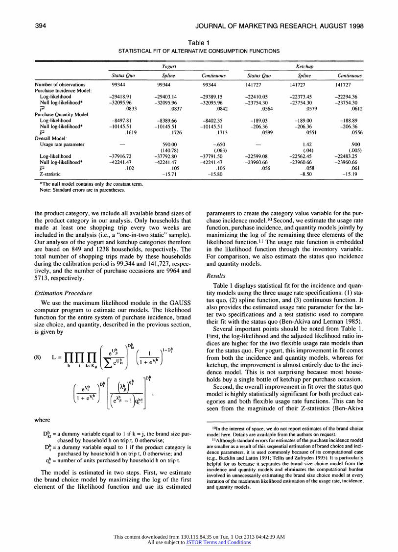
Table I displays statistical fit for the incidence and quantity models using the three usage rate specifications: (1) status quo, (2) spline function, and (3) continuous function. It also provides the estimated usage rate parameter for the latter two specifications and a test statistic used to compare their fit with the status quo (Ben-Akiva and Lerman 1985).

Several important points should be noted from Table 1. First, the log-likelihood and the adjusted likelihood ratio in- dices are higher for the two flexible usage rate models than for the status quo. For yogurt, this improvement in fit comes from both the incidence and quantity models, whereas for ketchup, the improvement is almost entirely due to the incidence model. This is not surprising because most households buy a single bottle of ketchup per purchase occasion.

Second, the overall improvement in fit over the status quo model is highly statistically significant for both product categories and both flexible usage rate functions. This can be seen from the magnitude of their Z-statistics (Ben-Akiva

where

Dht = a dummy variable equal to I if k = j, the brand size purchased by household h on trip t, 0 otherwise;

Dh = a dummy variable equal to I if the product category is purchased by household h on trip t, 0 otherwise; and

qh = number of units purchased by household h on trip t.

The model is estimated in two steps. First, we estimate the brand choice model by maximizing the log of the first element of the likelihood function and use its estimated

'In the interest of space, we do not report estimates of the brand choice model here. Details are available from the authors on request.

I ' Although standard errors for estimates of the purchase incidence model are smaller as a result of this sequential estimation of brand choice and incidence parameters, it is used commonly because of its computational ease (e.g., Bucklin and Lattin 1991; Tellis and Zufryden 1995). It is particularly helpful for us because it separates the brand size choice model from the incidence and quantity models and eliminates the computational burden involved in unnecessarily estimating the brand size choice model at every iteration of the maximum likelihood estimation of the usage rate, incidence, and quantity models.

394




and Lerman 1985). Therefore, we have strong evidence for the existence of a flexible usage rate, as well as convergent validity from both the spline and continuous functions.

Third, the estimated values of the usage rate parameters strongly support our hypotheses. For the continuous function, the estimated value of f is -.65 for yogurt and +.90 for ketchup.12 For the spline function, the estimated value of a is 590 for yogurt and 1.42 for ketchup. These parameter values confirm that the yogurt usage rate increases steadily with available inventory, whereas the ketchup usage rate is less sensitive to available inventory. The standard errors of the usage rate parameters for both product categories show that the difference in estimated values is statistically significant. Thus, we obtain strong discriminant validity for both usage rate functions. The value of a for yogurt, however, seems high. The reason for this is that some households have low values of Ch (e.g., .01 ounce) because they buy yogurt infre- quently. Even these infrequent users, however, consume most of their yogurt soon after purchasing it. A large a is the only way that the spline function can reflect this. This large a does not hurt model fit for frequent buyers because consumption is not allowed to exceed available inventory.

Fourth, the spline and continuous functions fit equally well in the yogurt category, but in the ketchup category, the continuous function is significantly better.13 Because consumption varies continuously with inventory, it also decreases continuously over the time between two purchases. For product categories with high flexibility (e.g., yogurt),

12As was expected, the value of the log-likelihood function for the status quo model is close to its value for our continuous usage rate model when the flexibility parameter f is set equal to 1.0.

13The spline function actually fits better for the yogurt quantity model, but this is offset by its poorer fit for the incidence model.

households quickly consume all they have, and inventory essentially goes down to zero. As we have seen previously, the spline can approximate this continuous function quite well by estimating an extremely large value for a. Similar- ly, the spline will work well for product categories with no flexibility because usage rate flattens out at Ch. However, for product categories with intermediate levels of flexibility (e.g., ketchup), for which consumption decreases gradually over time between two purchase occasions, this discontinu- ous function does not provide a good enough approximation to actual consumption.

In Table 2, we show estimates of the purchase incidence and quantity model for each product category using the status quo and the continuous flexible usage rate function.14 A comparison of the two sets of estimates shows that the key difference between them lies in the inventory parameter. Three of the four inventory parameters are much stronger when the flexible usage rate function is used, because it provides a better measure of household inventory than that obtained by the status quo model. The exception is the ketchup quantity model, which remains insensitive to inventory because, as we noted previously, most households buy a single unit of ketchup. Not surprisingly, the strengthening of the inventory parameter is much more dramatic in the case of yogurt. Yogurt consumption is highly flexible and the status quo model, by enforcing a constant consumption rate, intro- duces a large amount of measurement error in the inventory variable, thus biasing its coefficient strongly toward zero. When this measurement error is reduced through our flexible usage rate function, we obtain a less biased, stronger inventory parameter.

14Estimates using the spline function are similar.

Table 2 MODEL ESTIMATES UNDER ALTERNATIVE CONSUMPTION FUNCTIONS

Yogurt Ketchup

Flexible Usage Flexible Usage Variable Status Quo (Continuous) Status Quo (Continuous)

Purchase Incidence Estimates: Ch .271* .266* .989* .994*

(.007) (.005) (.022) (.023) Category value .050* .052* .062* .061*

(.018) (.018) (.020) (.021) Inventory -.0003* -.015* -.015* -.024*

(.0001) (.002) (.001) (.001) Lagged incidence 1.336* 1.412* -.110 .123**

(.027) (.028) (.072) (.073) Purchase Quantity Estimates:

Inventory .0001 * -.012* -.0005 -.0009

h_ (.00004) (.001) (.0004) (.002) Uh .156* .152* .318* .317*

(.004) (.003) (.053) (.081) Size purchased -.042* -.042* -.001 -.001

(.002) (.003) (.002) (.015) Price -3.277* -3.692* -1.201 -1.201

(.260) (.268) (1.404) (6.900) Promotion .133* .122* .021 .021

(.015) (.014) (.028) (.1 I1)

*p < .05. **p <. 10. Note: Standard errors are in parentheses.

395




Quantifying the Consumption Effect

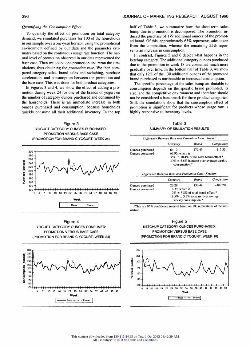
To quantify the effect of promotion on total category demand, we simulated purchases for 100 of the households in our sample over a one-year horizon using the promotional environment defined by our data and the parameter estimates based on the continuous usage rate function. The nat- ural level of promotion observed in our data represented the base case. Then we added one promotion and reran the simulations, thus obtaining the promotion case. We then compared category sales, brand sales and switching, purchase acceleration, and consumption between the promotion and the base case. This was done for both product categories.

In Figures 3 and 4, we show the effect of adding a promotion during week 24 for one of the brands of yogurt on the number of category ounces purchased and consumed by the households. There is an immediate increase in both ounces purchased and consumption, because households quickly consume all their additional inventory. In the top

Figure 3 YOGURT CATEGORY OUNCES PURCHASED:

PROMOTION VERSUS BASE CASE

(PROMOTION FOR BRAND C YOGURT, WEEK 24)

300 280 -

260 -

240 220 200 180 -

160 -

140 -

120 -

100 1 4 7 10 13 16 19 22 25 28 31 34 37 40 43 46 49

Week

| -- Base--- Promo [

Figure 4 YOGURT CATEGORY OUNCES CONSUMED:



- 280- 0 c 260- C = 240-

: 220- .2 200. E3 180.

= 160-

o 140- 0

120-

I

1 4 7 10 13 16 19 22 25 28 31 34 37 40 43 46 49

Week

I ,, Base ....... PromoI

half of Table 3, we summarize how the short-term sales bump due to promotion is decomposed. The promotion induced the purchase of 179 additional ounces of the promoted brand. Of this, approximately 65% represents sales taken from the competition, whereas the remaining 35% represents an increase in consumption.

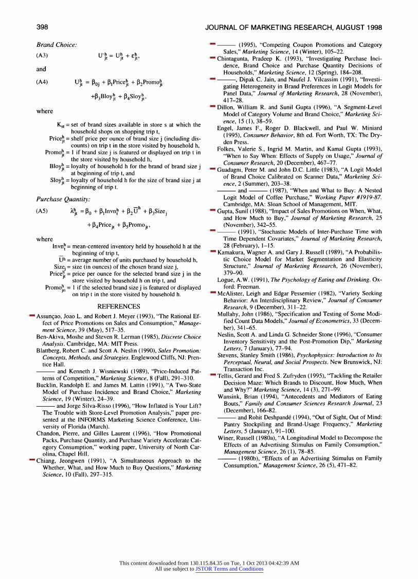
In contrast, Figures 5 and 6 depict what happens in the ketchup category. The additional category ounces purchased due to the promotion in week 18 are consumed much more gradually over time. In the bottom half of Table 3, we show that only 12% of the 130 additional ounces of the promoted brand purchased is attributable to increased consumption.

The specific percentage of the sales bump attributable to consumption depends on the specific brand promoted, its size, and the competitive environment and therefore should not be considered a benchmark for these product categories. Still, the simulations show that the consumption effect of promotion is significant for products whose usage rate is highly responsive to inventory levels.

Table 3 SUMMARY OF SIMULATION RESULTS

Difference Between Base and Promotion Case: Yogurt

Category Brand Competition

Ounces purchased 64.10 179.43 -115.33 Ounces consumed 63.96, which is

35% ? 10.4% of the total brand effect.* 30% ? 5.6% increase over average weekly

consumption.*

Difference Between Base and Promotion Case: Ketchup

Category Brand Competition

Ounces purchased 23.29 130.48 -107.20 Ounces consumed 16.39, which is

12% ? 5.8% of total brand effect.* 11.5% ? 3.3% increase over average

weekly consumption.*

*This is a 95% confidence interval based on 100 replications of the simulation.

Figure 5 KETCHUP CATEGORY OUNCES PURCHASED:



S

0

c

z

-S

0.

16 18 20 22 24 26 28 30 32 34 36 38 40 42 44 46 48 50

Week

|I --- Base ....... Promo I

396

i

0

f}

g.

o

IL

I Il.....lllllilIll........illII.

I4RM

,II IIIIIIIIII IIIIII IIIII III I III I II I1

' n \ Cxt-\s j / / aror vh




Figure 6 KETCHUP CATEGORY CONSUMPTION:



165

0 c

c 0

E

C c 0 0

160 -

155 -

150' -

145 I I I I I I I I I I 11 IIIIIi1111 IIIIII II 16 18 20 22 24 26 28 30 32 34 36 38 40 42 44 46 48 50

Week

jI -- Base ....... Promoj

DISCUSSION

In summary, we have accomplished the following in this article:

1. We have captured the usage rate mechanism by which promotion can increase category demand by modeling consumption during a given period as a function of inventory at the beginning of that period and incorporating this into a jointly estimated purchase incidence and quantity model. We have test- ed two different functional forms for this flexible usage rate.

2. We have estimated these models for two product categories, yogurt and ketchup, and shown that, in both cases, flexible usage rate functions fit significantly better than the status quo model. Convergent validity is evidenced by the ability of both functions to model the flexible usage rate phenomenon.

3. We have provided discriminant validity with the ability of both functions to estimate significantly different usage rate parameters for the less flexible ketchup category and the more flexible yogurt category.

4. We have demonstrated the importance of the flexible usage rate phenomenon by quantifying the effect of promotion on consumption through a Monte Carlo simulation. For yogurt, for which usage rate is highly flexible, a substantial percentage of the short-term promotion sales bump is attributable to increased category consumption.

Implications for Researchers and Managers There are several implications of these results for

researchers. First, and most basic, flexible consumption is a real phenomenon that provides a fertile area for marketing science modeling. There are many more issues to investigate. For example, which product categories are more or less prone to flexible consumption and why? We believe our results illustrate the promise of undertaking such work.

Second, our flexible usage rate functions appear to capture the phenomenon quite well with only one parameter. The continuous function is preferred because it fits as well as the spline in one category and significantly better in the other. However, there are various avenues along which these functions could be improved. For example, the parameters in the two usage rate functions, a and f, could be

functions of price expectations and/or depend on various de- mographics, such as household size and income level. Re- searchers also could investigate household heterogeneity in these parameters by splitting the data by demographic group and estimating a separate parameter for each or by using one of several methods of modeling unobserved heterogeneity (e.g., Chintagunta, Jain, and Vilcassim 1991; Kamakura and Russell 1989).

Third, we need to understand the behavioral underpin- nings of flexible consumption in more detail. For example, our model establishes a strong link between inventory and consumption, but it does not address whether households jointly optimize inventory and consumption levels or whether promotion leads them to stockpile, and they then use additional inventory at a faster rate then usual. Further research is required to disentangle the two, through either econometric modeling or experimental work. It also would be valuable to develop a comprehensive utility maximiza- tion framework that brings together work on optimal purchase decisions (e.g., Chiang 1991; Chintagunta 1993) with work on optimal consumption decisions (e.g., Assuniao and Meyer 1993).

Our work also has important implications for managers. Managers should not view promotion as only a market share or temporal displacement game. It can be used to grow the category. This is particularly important for managers of high share brands, who often view promotion as unprofitable because they cannot attract a greater share. As we have shown, this depends on the product category. Sta- ples such as bathroom tissue, diapers, and various cleaning products might be difficult to expand with promotion. But for many other categories-yogurt, cereal, cookies, bever- ages, and so forth-managers should think of promotion as a tool for growing the category rather than as a market share weapon. Finally, there also might be some important public health and policy implications of this research, espe- cially as it relates to consumption of food items and diet control.

APPENDIX

Variables in Incidence, Choice, and Quantity Models

Purchase Incidence:

(Al) 'h= h + ' t "t t ,

and

(A2) Vh = 30o + P1CatValh + I21nvnh

+ P3C +f 34Purlnct -,

where

CatValh = category value for household h during week t (equal to the "inclusive value" of nested logit, obtained from the brand choice model),

Invnh = mean-centered inventory held by household h at _ beginning of week t,

Ch = average daily consumption for household h, equal to total amount purchased over the period divided by number of days, and

Purlnch_ = dummy variable equal to 1 if product category was purchased during previous shopping trip and 0 if not.

397

_e/~~~~~~~~~~~~F.-




u,' = Uh + e jt jit Jt

and

(A4) Uht = Poj + 31Priceht + 12Promot

+P3Bloyht + P4Sloyht,

where

KSt = set of brand sizes available in store s at which the household shops on shopping trip t,

Priceh = shelf price per ounce of brand size j (including dis- counts) on trip t in the store visited by household h,

Promoh = I if brand size j is featured or displayed on trip t in the store visited by household h,

Bloyht = loyalty of household h for the brand of brand size j at beginning of trip t, and

Sloyh = loyalty of household h for the size of brand size j at beginning of trip t.

Purchase Quantity:

(A5) Xt =P0 + Pil1nvnt + P2U + h3Sizej

+ P4Pricejt + P5Promojt,

where Invnh = mean-centered inventory held by household h at the

beginning of trip t, Uh = average number of units purchased by household h,

Sizej = size (in ounces) of the chosen brand size j, Price1O = price per ounce for the selected brand size j in the

store visited by household h on trip t, and Promohn = I if the selected brand size j is featured or displayed

on trip t in the store visited by household h.

REFERENCES

Assunqao, Joao L. and Robert J. Meyer (1993), "The Rational Ef- fect of Price Promotions on Sales and Consumption," Manage- ment Science, 39 (May), 517-35.

Ben-Akiva, Moshe and Steven R. Lerman (1985), Discrete Choice Analysis. Cambridge, MA: MIT Press.

Blattberg, Robert C. and Scott A. Neslin (1990), Sales Promotion: Concepts, Methods, and Strategies. Englewood Cliffs, NJ: Pren- tice Hall.

and Kenneth J. Wisniewski (1989), "Price-Induced Pat- terns of Competition," Marketing Science, 8 (Fall), 291-310.

Bucklin, Randolph E. and James M. Lattin (1991), "A Two-State Model of Purchase Incidence and Brand Choice," Marketing Science, 19 (Winter), 24-39.

and Jorge Silva-Risso (1996), "How Inflated is Your Lift? The Trouble with Store-Level Promotion Analysis," paper pre- sented at the INFORMS Marketing Science Conference, Uni- versity of Florida (March).

Chandon, Pierre, and Gilles Laurent (1996), "How Promotional Packs, Purchase Quantity, and Purchase Variety Accelerate Cat- egory Consumption," working paper, University of North Car- olina, Chapel Hill.

Chiang, Jeongwen (1991), "A Simultaneous Approach to the Whether, What, and How Much to Buy Questions," Marketing Science, 10 (Fall), 297-315.

(1995), "Competing Coupon Promotions and Category Sales," Marketing Science, 14 (Winter), 105-22.

Chintagunta, Pradeep K. (1993), "Investigating Purchase Inci- dence, Brand Choice and Purchase Quantity Decisions of Households," Marketing Science, 12 (Spring), 184-208.

, Dipak C. Jain, and Naufel J. Vilcassim (1991), "Investi- gating Heterogeneity in Brand Preferences in Logit Models for Panel Data," Journal of Marketing Research, 28 (November), 417-28.

Dillon, William R. and Sunil Gupta (1996), "A Segment-Level Model of Category Volume and Brand Choice," Marketing Sci- ence, 15 (1), 38-59.

Engel, James F., Roger D. Blackwell, and Paul W. Miniard (1995), Consumer Behavior, 8th ed. Fort Worth, TX: The Dry- den Press.

Folkes, Valerie S., Ingrid M. Martin, and Kamal Gupta (1993), "When to Say When: Effects of Supply on Usage," Journal of Consumer Research, 20 (December), 467-77.

Guadagni, Peter M. and John D.C. Little (1983), "A Logit Model of Brand Choice Calibrated on Scanner Data," Marketing Sci- ence, 2 (Summer), 203-38.

and (1987), "When and What to Buy: A Nested Logit Model of Coffee Purchase," Working Paper #1919-87. Cambridge, MA: Sloan School of Management, MIT.

Gupta, Sunil (1988), "Impact of Sales Promotions on When, What, and How Much to Buy," Journal of Marketing Research, 25 (November), 342-55.

(1991), "Stochastic Models of Inter-Purchase Time with Time Dependent Covariates," Journal of Marketing Research, 28 (February), 1-15.

Kamakura, Wagner A. and Gary J. Russell (1989), "A Probabilis- tic Choice Model for Market Segmentation and Elasticity Structure," Journal of Marketing Research, 26 (November), 379-90.

Logue, A.W. (1991), The Psychology of Eating and Drinking. Ox- ford: Freeman.

McAlister, Leigh and Edgar Pessemier (1982), "Variety Seeking Behavior: An Interdisciplinary Review," Journal of Consumer Research, 9 (December), 311-22.

Mullahy, John (1986), "Specification and Testing of Some Modi- fied Count Data Models," Journal of Econometrics, 33 (Decem- ber), 341-65.

Neslin, Scott A. and Linda G. Schneider Stone (1996), "Consumer Inventory Sensitivity and the Post-Promotion Dip," Marketing Letters, 7 (January), 77-94.

Stevens, Stanley Smith (1986), Psychophysics: Introduction to Its Perceptual, Neural, and Social Prospects. New Brunswick, NJ: Transaction Inc.

Tellis, Gerard and Fred S. Zufryden (1995), 'Tackling the Retailer Decision Maze: Which Brands to Discount, How Much, When and Why?" Marketing Science, 14 (3), 271-99.

Wansink, Brian (1994), "Antecedents and Mediators of Eating Bouts," Family and Consumer Sciences Research Journal, 23 (December), 166-82.

and Rohit Deshpand6 (1994), "Out of Sight, Out of Mind: Pantry Stockpiling and Brand-Usage Frequency," Marketing Letters, 5 (January), 91-100.

Winer, Russell (1980a), "A Longitudinal Model to Decompose the Effects of an Advertising Stimulus on Family Consumption," Management Science, 26 (1), 78-85.

(1980b), "Effects of an Advertising Stimulus on Family Consumption," Management Science, 26 (5), 471-82.

Brand Choice:

(A3)

398



ailawadi, k. l., & neslin, s. a. (1998). the effect of promotion on consumption- buying more and...

Documents

category consumption

consumption rates

ketchup consumption

effect of promotion

consumption stems

consumption effects

effect of sales promotion

jstor terms