Air Entrainment and Acoustic Wave Celerities Following a Rapidly Moving Pipe FillingBore

by

Andrew Patrick

A thesis submitted to the Graduate Faculty ofAuburn University

in partial fulfillment of therequirements for the Degree of

Master of Science

Auburn, AlabamaMay 10, 2015

Keywords: Pipeline Priming, Air Entrainment, Rapid Filling, Pipe filling bore, Acoustic wave,Water hammer

Copyright 2015 by Andrew Patrick

Approved by

Jose Goes Vasconcelos Neto, Professor of Civil EngineeringPrabakhar Clement, Professor of Civil Engineering

Xing Fang, Professor of Civil Engineering

Abstract

Water mains stormwater sewers and tunnels may undergo processes of rapid filling, in which

flow regimes transit from open channel into pressurized flows. In the process, air bubbles may

be entrained, which may influence the resulting volume and distribution of air in the system upon

priming. The amount of air that is entrained can have an effect on the the magnitude of the pressure

wave celerities, an important parameter in the numerical simulation of unsteady tunnel filling or

pipeline priming. However, air entrainment has not yet been studied in the context of rapid filling

pipe flows. The purpose of this research is to study the nature of air entrainment and the effects on

the celerity of pressure waves following episodes of rapidly filling pipes. Studies were conducted

on a 10-m long, 1% and 2% slope, clear PVC pipeline using three diameters ranging from 50 mm

to 152 mm. Inflow rates were systematically varied, and various repetitions (at least 10) were

performed in each case to ensure consistency of results. Air entrainment is initiated by creating

a backward moving, sometimes pipe-filling bore generated by a knife-gate valve closure at the

down stream end. Upon complete pipe pressurization and air entrainment, a second pressure pulse

was generated by maneuvering a solenoid valve. After each run the amount of air entrained is

measured, as well as the speed of the acoustic wave and the speed of the bore. Research results

include analyzing the relationship between the volume of air entrainment and various normalized

parameters. The acoustic wave speed in these tests were also compared to baseline cases in which

no air was entrained. These experiments hope to improve current understanding of unsteady flows

following the rapid filling of closed pipes.

ii

Acknowledgments

I would like to thank my advisor and friend, Professor Jose Goes Vasconcelos, for all the

patience and time spent in the development of my experimental research. Your good counsel and

academic mentoring was vital in the development of my engineering knowledge base. I also would

like to thank Robyn Manhard for the help in the laboratory with the experiments. I would also like

to thank my fiancee Kimberly for her patience and encouragement throughout my tenure here at

Auburn. A good woman is an enabler, I am thankful for your faith in me.

I would like also to thank my parents, Scott (Dad) and Carmen (Mom) Patrick, as well as my

brother, Aaron, and sister, Maggie as well as my extended family for being my rock solid support

system.

I would finally like to thank the Lord for his providence and guidance. This document has

been a long time coming and he has been faithful. ”And let us not grow weary of doing good, for

in due season we will reap, if we do not give up” Galatians 6:9

iii

Table of Contents

Abstract . . . . . . . . . . . . . . . . . . . . . . . . . . . . . . . . . . . . . . . . . . . . . ii

Acknowledgments . . . . . . . . . . . . . . . . . . . . . . . . . . . . . . . . . . . . . . . . iii

List of Figures . . . . . . . . . . . . . . . . . . . . . . . . . . . . . . . . . . . . . . . . . . vi

List of Tables . . . . . . . . . . . . . . . . . . . . . . . . . . . . . . . . . . . . . . . . . . viii

1 Introduction . . . . . . . . . . . . . . . . . . . . . . . . . . . . . . . . . . . . . . . . 1

2 Literature Review . . . . . . . . . . . . . . . . . . . . . . . . . . . . . . . . . . . . . 3

2.1 Air entrainment in classical free surface hydraulic jumps . . . . . . . . . . . . . . 3

2.2 Air pocket formation and behavior . . . . . . . . . . . . . . . . . . . . . . . . . . 6

2.3 Air Removal from Pipelines . . . . . . . . . . . . . . . . . . . . . . . . . . . . . 7

2.4 Air entrainment in closed conduits . . . . . . . . . . . . . . . . . . . . . . . . . . 9

3 Knowledge Gap and Objectives . . . . . . . . . . . . . . . . . . . . . . . . . . . . . . 15

4 Methodology . . . . . . . . . . . . . . . . . . . . . . . . . . . . . . . . . . . . . . . 16

4.1 Apparatus Description . . . . . . . . . . . . . . . . . . . . . . . . . . . . . . . . 16

4.2 Experimental Procedure . . . . . . . . . . . . . . . . . . . . . . . . . . . . . . . . 19

4.3 Data Collection . . . . . . . . . . . . . . . . . . . . . . . . . . . . . . . . . . . . 22

4.4 Troubleshooting . . . . . . . . . . . . . . . . . . . . . . . . . . . . . . . . . . . . 24

4.5 Error . . . . . . . . . . . . . . . . . . . . . . . . . . . . . . . . . . . . . . . . . . 28

5 Results and analysis . . . . . . . . . . . . . . . . . . . . . . . . . . . . . . . . . . . . 29

5.1 Froude Comparison . . . . . . . . . . . . . . . . . . . . . . . . . . . . . . . . . . 31

5.2 Normalized Flow and Air Entrainment . . . . . . . . . . . . . . . . . . . . . . . . 45

5.3 Gravity Currents . . . . . . . . . . . . . . . . . . . . . . . . . . . . . . . . . . . 46

5.4 System Priming Rate . . . . . . . . . . . . . . . . . . . . . . . . . . . . . . . . . 50

5.5 Acoustic Wave Celerities . . . . . . . . . . . . . . . . . . . . . . . . . . . . . . . 52

iv

6 Conclusion . . . . . . . . . . . . . . . . . . . . . . . . . . . . . . . . . . . . . . . . 55

Bibliography . . . . . . . . . . . . . . . . . . . . . . . . . . . . . . . . . . . . . . . . . . 58

v

List of Figures

2.1 Image (a)-(d) show, respectively, a hydraulic jump with undulations Fr = 1.1, a directhydraulic jump Fr = 2.3, a hydraulic jump with recirculations Fr = 4.1, and a hydraulicjump with transition to pressurized flow Fr = 6.5. . . . . . . . . . . . . . . . . . . . . 5

2.2 The plot for β vs. Froude number taken from Kalinske and Robertson [1943]. . . . . . 10

2.3 Experimental data presented by Mortensen et al. [2011]. The pipe diameters are asfollows in (cm); � 7.62,� 17.7, ◦ 30.0, N 59.1. The bold line is the proposed equationby Mortensen et al. [2011] and the other is Kalinske and Robertson [1943] . . . . . . . 12

2.4 The three cases and locations for hydraulic jumps tested by Mortensen et al. [2012] inwhich Lr = length of roller, Lj = length of jump and La = length of aeration. . . . . . . 13

4.1 A view of the 102 mm configuration looking upstream . . . . . . . . . . . . . . . . . 17

4.2 The apparatus used to run the experiments . . . . . . . . . . . . . . . . . . . . . . . . 17

4.3 Shows the valve combination progression repeated for each experimental run. 1.Steady state: Knife gate open, solenoid closed 2. Bore Generation: Knife gate closed,solenoid closed 3. Pressure wave Generation: Knife gate closed, solenoid open 4.Pressurization: Knife gate closed, solenoid closed. . . . . . . . . . . . . . . . . . . . 21

4.4 Typical pressure signal used to calculate the acoustic wave speed after being passedthrough a numerical filter. . . . . . . . . . . . . . . . . . . . . . . . . . . . . . . . . 21

4.5 This figure shows how the non-visible portion of the PVC pipe was dimensioned.The hatched area is the water inside the pipe with the air pocket on top. A tape wasprojected along the waters surface to the back of the PVC elbow to determine theellipsoid depth. . . . . . . . . . . . . . . . . . . . . . . . . . . . . . . . . . . . . . . 23

4.6 The USB conversion for the pressure transducers . . . . . . . . . . . . . . . . . . . . 26

5.1 The three scenarios observed during the experimental testing. . . . . . . . . . . . . . . 29

5.2 The Froude number compared with β where β is the air entrained divided be the timerequired for the bore to sweep the system. . . . . . . . . . . . . . . . . . . . . . . . . 32

5.3 Froude number compared with V ∗A for both 1% and 2% slopes. Each point is an aver-age of repetitions. . . . . . . . . . . . . . . . . . . . . . . . . . . . . . . . . . . . . . 35

5.4 A frame taken from the camera of the case 2 bore seen in the 6 in pipe. The top imageis the bore advancing and the bottom shows after the bore has passed . . . . . . . . . . 36

5.5 Both pipes have the same Q∗, the top image has a 1% slope with Fr. = 1.4 and thebottom image has a 2% slope and Fr. = 2.6 . . . . . . . . . . . . . . . . . . . . . . . 37

vi

5.6 Bubbles collected along the roof of the pipe following a weak bore that caused lapping. 38

5.7 An image sample from each series of repetitions run for 50 and 102 mm pipe diametersat 1% slope . . . . . . . . . . . . . . . . . . . . . . . . . . . . . . . . . . . . . . . . 41

5.8 An image sample from each series of repetitions run for the 152 mm pipe diameter at1% slope . . . . . . . . . . . . . . . . . . . . . . . . . . . . . . . . . . . . . . . . . 42

5.9 An image sample from each series of repetitions run for 50 and 102 mm pipe diametersat 2% slope . . . . . . . . . . . . . . . . . . . . . . . . . . . . . . . . . . . . . . . . 43

5.10 An image sample from each series of repetitions run for the 152 mm pipe diameters at1% slope . . . . . . . . . . . . . . . . . . . . . . . . . . . . . . . . . . . . . . . . . 44

5.11 The normalized flow rate compared with V ∗A . Each point is an average of repetitions. . 46

5.12 The normalized bore velocity compared with V ∗A . . . . . . . . . . . . . . . . . . . . . 47

5.13 The ratio of the bores interface to diameter of the pipe for both 1% and 2%. Error barsare show .25D because lengths were estimated . . . . . . . . . . . . . . . . . . . . . 49

5.14 This figure shows how the parameter L f was estimated. The black tape lines are spacedat 152-mm intervals. . . . . . . . . . . . . . . . . . . . . . . . . . . . . . . . . . . . 50

5.15 The normalized time compared with V ∗A . Each point is an average of repetitions. . . . . 51

5.16 The normalized acoustic wave celerities compared with V ∗A . This chart also containsthe theoretical values for pipe size and entrainment. . . . . . . . . . . . . . . . . . . . 53

vii

List of Tables

4.1 List of the various electrical components used as well as their operational limits. . . . 18

4.2 Component sizes for various experimental runs . . . . . . . . . . . . . . . . . . . . . 18

4.3 Detailed flow rates for each series of test . . . . . . . . . . . . . . . . . . . . . . . . . 24

4.4 Estimated Error of Measurements . . . . . . . . . . . . . . . . . . . . . . . . . . . . 28

viii

List of Notations

a = Corresponding number to value n Escarameia [2007]aair = Calculated acoustic wave speed based on equations Wylie and Streeter [1993]aw = Calculated acoustic wave speed based on equations Wylie and Streeter [1993]

A f s = Area of the free surface flowAvoid = Area of the pipe without water

β = Ratio of Air to Water flow rateB∗v = Normalized Bore Velocity

Bvel = Velocity of the boreC∗ = Normalized Acoustic Wave Speed

Cbaseline = Measured acoustic wave speed with no air in the systemCmeasured = Measured acoustic wave speed in the pipe

Ct = Normalized acoustic wave celerity based on theoretical valuesD = Pipeline diameterE = Youngs modulus of the pipe materiale = Pipe wall thickness

V ∗A = Normalized Air EntrainmentFr = Froude Number

g = Gravity accelerationK = Bulk modulus of elasticity for the system

Kg = Bulk modulus of elasticity of airKliq = Bulk modulus of elasticity of waterL f = The length of the air water interface of the bore

Lpipe = Total pipeline lengthQ∗ = Normalized flow rate in the pipeline=Qin f low/

√gD5

n = 4VbubbleπD3

Qin f low = Measured flow rateρ = Density of air-water mixture

ρg = Density of airρliq = Density of liquid

s = Slope of the pipeS f = Correction factor (≈ 1.1) Escarameia [2007]T = Total time taken for the bore to sweep the system.

SPR = Normalized variable accounting for length, diameter, and duration timeTwidth = Top width of the free surface flow

V ∗A = Normalized entrained air volumeVair = Volume of air

Vbubble = Volume of an air bubbleVclear = Velocity required to clear an air pocket from a line

Vliq = Volume of liquid in the systemVg = Volume of air in the systemV = Volume of air and liquid in the system

ix

Chapter 1

Introduction

The rapid filling of water conveyance systems, whether they be storm water or water works

transmission lines, can often entrain air through the mechanics of a hydraulic jump. The entrain-

ment process happens at the turbulent interface where water changes from a supercritical flow

profile to a sub-critical flow profile. This transition also happens in free surface flows such as

open channel energy dissipation devices. This topic has practical importance since it has been

established that entrained air in closed conduits has a strong impact in decreasing the speed of

the acoustic wave, thus decreasing the strength of water hammer phenomena [Wylie and Streeter,

1993]. Knowledge of air entrainment in closed conduits caused by hydraulic jumps are also rele-

vant in the context of air-water surges and water hammer phenomena in pipelines once these sys-

tems are operating in pressurized conditions. Because air in pipelines has adverse effects, pipeline

efficiency and improved understanding of the ways that air enters a pipeline during the priming

process could lead to safer operations of distribution systems.

Previous researchers have investigated the characteristics and mechanics of air entrainment

in static hydraulic jumps. Such research has established that conduit geometry, Froude num-

ber, Reynolds numbers, and viscous forces contribute to the quantity of air entrained in hydraulic

jumps. Past investigations have also helped to explain the formation of pockets of air in pipelines

as well as their behavior, motion, and contributions to pipeline pressure fluctuations. These stud-

ies cover a variety of surcharging conditions that can lead to air pocket formation and were both

experimental and observational in nature.

The first publication documenting air entrainment from a hydraulic jump in a closed conduit

was presented by Kalinske and Robertson [1943]. Since then there have been several papers ex-

ploring additional parameters that influence air entrainment caused by a hydraulic jump in a closed

1

conduits. Yet, no investigation to date has considered the case of a moving bore and its effects

during the priming of a pipeline.

This thesis presents a experimental investigation on air entrainment caused by a moving bore

by testing a variety of pipe diameters and flow rates on different slopes. The experimental apparatus

and procedure are presented and supported with figures and images to clarify the processes. The

data and results are also discussed using a variety of normalized parameters in order to assess the

applicability of those findings to other commentaries. Such parameters provide interesting insights

on the phenomenon and the collected data, consequential results, and discussion.

2

Chapter 2

Literature Review

Investigations to date involving static pipe-filling bores in closed conduits have determined

that such jumps create significant air entrainment which increases with the Froude number mea-

sured at the toe of the jump. A similar investigation of the nature of entrainment in rapid filling

pipe conditions, where hydraulic jumps and pressurization interfaces are not static, has not been

performed to date. The following literature review will be an overview of works that investigate

air entrainment in classical hydraulic jumps, air pocket formations and behavior in pressurized

pipelines, hydraulic removal of air from pipelines, and finally a review of studies involving air

entrainment via a hydraulic jump in closed conduits.

2.1 Air entrainment in classical free surface hydraulic jumps

Air entrainment in hydraulic jumps is a significant mode by which air enters flow profiles.

Studies investigating the amount of air entrained in a classical free surface hydraulic jump is inves-

tigated and explained by Rajaratnam [1962]; Hager and Bremen [1989]; Chanson [2006]. Chanson

and Murzyn [2008]; Chanson and Gualtieri [2008]; Gualtieri and Chanson [2007]; Chanson [2006,

1995] are all studies addressing scale effects for air entrainment in a hydraulic jumps. These studies

suggested that air entrainment is effected by geometric properties of the jump by showing discrep-

ancies in air entrainment for jumps that were dynamically similar. By comparing two jumps with

similar Froude numbers and different flume widths, it was noticed that larger jumps entrained more

air. This was attributed this to the higher velocities in the larger jumps [Chanson and Gualtieri,

2008].

These experimental studies also attributed bubble size to the amount of air entrained. One

study by Chanson and Gualtieri [2008] found that stronger hydraulic jumps created smaller bubbles

3

because the strength of the vorticies in the larger jump were able to break larger air pockets into

smaller ones that are more easily entrained and swept downstream. The work by Chanson and

Murzyn [2008] compared air entrainment to many different normalized parameters and found that

Froude similitude does not always best explain air entrainment. These previous studies suggested

that viscous and tension forces also contribute to the quantity of air entrainment.

Studies by Hager and Bremen [1989, 1990] added to the discussion of the classical free sur-

face hydraulic jump. Their works described jump characteristics by observing the region of tur-

bulent recirculation. Their works defined a roller length and aeration length. The roller length

was considered the distance from the toe of the jump to where the surface flow velocity is zero

described in the paper as the stagnation point. The aeration length was considered the length from

the toe of the jump to where the bubbles had reached the surface. The same studies done by Hager

and Bremen [1990] and Hager and Bremen [1989] found that the Reynolds number in addition

to the Froude number has an impact on air entrainment in hydraulic jumps for Froude numbers

greater than 8.

A transitional study from free surface hydraulic jumps to those in closed conduits was con-

ducted by Stahl and Hager [1999]. This study, while not pertaining to air demand or quantification

of air mass entrained, looked at the subsequent depths of a hydraulic jump in a closed conduit. The

purpose of this observational study was to discuss pre-jump flow conditions that would create a

hydraulic jump where the subsequent depth was less than the diameter of the conduit. These find-

ings showed that hydraulic jumps with subsequent depths less than the pipe diameter had similar

properties to that of a free surface hydraulic jump. This same work reported observed properties

of various jumps in closed conduits. Stahl and Hager [1999] noted that in jumps with a filling

ratio of h/D > (1/3), where h is the depth of the water at the toe of the jump and D is the pipe

diameter, the hydraulic jumps width was similar to the that the supercritical free surface flow prior

to the jump. This work also noted that the hydraulic jump is similar to a classical hydraulic jump

in terms of the development of rollers and a length of aeration. This work also noted that for jumps

with a h/D ratio smaller than (1/3) the jump developed wings. These wings are described as areas

4

Figure 2.1: Image (a)-(d) show, respectively, a hydraulic jump with undulations Fr = 1.1, a directhydraulic jump Fr = 2.3, a hydraulic jump with recirculations Fr = 4.1, and a hydraulic jump withtransition to pressurized flow Fr = 6.5.

5

of circulating flow on either side of the main entry flow or jet. These wings are similar in depth to

that of the entry flow but essentially expand the channel into the surcharging interface of the jump.

These two types of jumps were noticed in flows with a Froude number greater than 2. More impor-

tantly however, Stahl and Hager [1999] noticed that for Froude numbers less than 2 the jumps in

the closed conduit were undular meaning that it was characterized by irregularities in the surface

such as waves. The images of the different cases presented in by Stahl and Hager [1999] can be

seen in Figure 2.1. The images (a) and (b) in this figure are the experiments with similar Froude

numbers used in this thesis.

Although all of these studies are relevant in the understanding of air entrainment in hydraulic

jumps, none of these studies dealt with a moving bore.

2.2 Air pocket formation and behavior

Other studies have also looked into different mechanisms whereby air becomes entrapped

during the filling of closed conduits. Research conducted by Hamam and McCorquodale [1982]

explored methods of air pocket formation based on shear forces developed from air movement

across a free surface flow. His research looked at the development of irregularities in the free

surface caused by shear from an air current that flowed counter current the the free surface below

in a closed conduit. As these water surface irregularities grew, they eventually reached to the crown

of the conduit developing a pressurized air pocket.

Additional research pertaining to the behavior of these air pocket are explored as gravity

currents. A classic publication by Benjamin [1968] addresses the velocities of gravity currents in

near horizontal pipelines as they progress forward. Benjamin [1968] found this maximum value to

be v/(gD)0.5 = 0.54, Corcos [1992] later found the value to be v/(gD)0.5 = 0.484 for smaller near

horizontal pipes. Where v is the gravity current velocity, g is gravity and D is the pipe diameter.

An additional study by Baines [1991] explained the gulping phenomenon in a horizontal pipe as it

relates to gravity currents. He found that this gulping, similar to the gulping noticed when pouring

out a water bottle, occurred in horizontal pipes with a weir or partial obstruction at the outlet.

6

Another publication by Zhou et al. [2002] discussed the effects of pressure oscillations in a

pipe segment when a pocket of air was compressed by an advancing water front with an orifice at

the end. His research was in the movement of the air/water interface as the mass (air and water)

in the pipe was expelled through the down stream orifice. His work aided in the explanation of air

pocket formation in poorly ventilated pipelines. Another similar study by Vasconcelos and Wright

[2006] looked at how air pockets move in a horizontal pipeline with different inflows. Although

the paper by Vasconcelos and Wright [2006] was strictly observational, it did shed light on the

advancing front during the surcharging of a water line.

None of these above studies however addressed air entrainment in a closed conduit via means

of a hydraulic jump but rather the formation of large air pockets from a rapidly advancing surcharge

interface.

2.3 Air Removal from Pipelines

Many authors have investigated methods for removing air from pipelines via hydraulic means.

This process is often referred to as hydraulic clearing. A paper by Wisner et al. [1975] presented

initial works by previous authors. The purpose of his paper was to replicate and discuss the findings

of previous authors who investigated hydraulic clearing of air in pipelines. The earliest of these

studies reference by Wisner et al. [1975] was the paper by Gandenberger [1957]. Another paper

more recently published explaining previous works was that of Lauchlan et al. [2005]. This report

presented many previous researchers contributions to air pocket and air bubble behavior and move-

ment in pipelines including air removal. Escarameia [2007] published a study in which she looked

into the removal of air bubbles in a pipeline of various slopes ranging from 0 to 22.5◦downward

as well as some upward slopes. Her work consisted of a 150 mm diameter pipe into which she

introduced air and observed its behaviors as well as the minimum velocity required to overcome

surface tension and buoyant forces on the bubble to drive it downstream. The focus of her research

was on milder slopes similar to those used in this current study. There is an equation proposed by

7

Escarameia [2007] for clearing velocities for a bubble based on her experimental study and it can

be seen as follows:

Vclear = S f (g ·D)0.5 ∗ [0.56 · sin(s)0.5 +a] (2.1)

Where Vclear is the minimum velocity needed to clear a bubble, S f is a safety factor that is 1.1,

s is the slope, a is a variable that corresponds to an n value that is an expression of air volume to

pipe diameter. A more recent study by Pozos et al. [2010] sought to validate equations proposed

by previous researchers. His findings were that for pipes with slopes ranging from 0.087 to 1.73 air

bubble movement upstream or downstream based on flow rate and diameter was correctly predicted

by the equation:

Q2in f low

g ·D5 = s (2.2)

Where Qin f low is the inflow rate, g is gravity, D is the pipe diameter, and s is the pipe slope. If

the left hand side of the equation is greater than the right then the air pocket will move in the water

flow direction. If the opposite is true then the air pocket will move against the flow. This paper

by Pozos et al. [2010] was discussed by a paper Falvey [2011] that disputed Pozos et al. [2010]

findings based on failures of hydraulic structures incurred by the USBR. Falvey [2011] stated

that while the findings by Pozos et al. [2010] may apply to small bubbles and air pockets, real

water conveyance systems can have multidirectional air flow based on pocket size and distribution.

These small pockets can collect downstream into bigger pockets that eventually become buoyant

enough to blow back upstream against the flow. Falvey [2011] presented a plot showing instances

of conditions where the equation validated by Pozos et al. [2010] determined air pockets were to be

swept downstream but instead a blowback occurred that damaged a USBR hydraulic conveyance

unit.

The discussion of air removal in pipelines via hydraulic means has been investigated by many

authors. There have been investigations looking into viscus forces, scale effects, and the effects of

8

slope on air pocket removal. While this is not the focus of this research, a background in hydraulic

clearing can help to further discuss the air pocket behavior in this study.

2.4 Air entrainment in closed conduits

The amount of air that can be entrained in a static hydraulic jump occurring within a closed

conduit was first investigated in a 1943 study by Kalinske and Robertson presented by Falvey

[1980]. That pioneering work explored the air demand in closed conduit flows where a hydraulic

jump is present, and the results scaled reasonably well with the Froude number at the toe of the

jump. Kalinske and Robertson [1943] experiments involved measuring the air demand for a hy-

draulic jump in a closed conduit for slopes ranging from 0 to 16 degrees. Their findings were that

the level of air demand for entrainment in the jump was a function of the Froude number at the toe

of the jump. The study proposed an equation for β , which was the ratio of water flow rate, Qin f low,

and the volumetric flow rate of entrained air, Qair:

β =Qair

Qin f low= 0.0066(Fr−1)1.4 (2.3)

A plot of data presented by Kalinske and Robertson [1943] can be seen in Figure 2.2. As in-

dicated in equation 2.3, entrainment increased with the Froude number, Fr, measured at the toe of

the hydraulic jump. Kalinske and Robertson [1943] also noted that in much steeper slopes, it was

possible for more than one hydraulic jump to occur over the length of the pipe. An important phe-

nomenon, referred to as “blow-back”, and characterized by the return of entrained air mass toward

the jump, was not reported by the authors, as pointed by Falvey [1980], Estrada [2007] and Sherma

[1967]. Sherma [1967] collected air entrainment data for a high head gated conduit that was rect-

angular. His experiments tested many different pipe filling flow scenarios including those which

generated a stationary bore that filled the rectangular conduit. Sherma [1967] found that the model

proposed by Kalinske and Robertson [1943] underestimated air entrainment when the hydraulic

9

Figure 2.2: The plot for β vs. Froude number taken from Kalinske and Robertson [1943].

10

jumps location was a significant distance away from the pipe entrance. He did suggest however

that jump location and upstream roughness in the water surface could effect air entrainment.

Escarameia [2007] performed similar experiments to that of previous researchers except that

her experiments used a circular conduit rather than a rectangular one. A section of this paper

discussed the applications of air evacuation through hydraulic jumps. The data presented in Es-

carameia [2007] compares the previous works of Kalinske and Robertson [1943], Wisner et al.

[1975], Rajaratnam [1967], and Rabben et al. [1983] in a plot with the results of her experimental

investigation. Her work revealed large discrepancies in the data found by the different authors.

She contributed this to a jump that emptied into a full pipe flow rather than exited into a free sur-

face flow as well as the shape of the conduit being circular rather than rectangular. Escarameia

[2007] showed that conduit shape matters when quantifying the amount of air entrained by a hy-

draulic jump in a closed conduit. A later study by Pothoff [2011] would expand on the use of these

parameters to predict air movement and behavior in pipes.

A recent investigation by Mortensen et al. [2011] focused on the scale effects of different

pipe sizes and water temperatures on air entrainment in static pipe-filling bores. To do this the

researchers selected several different diameter pipes made of both steel and acrylic. All test were

performed at a slope of 4%. To measure the amount of air entrained in the various jumps, an air

velocity sensor was placed at the air intake on the upstream end of the pipe. To ensure that the size

of the air intake valve did not choke the amount of air entrained, several different size intakes were

used to show that the air flow was consistent. Test were run for different diameter pipes ranging

from 7.62 to 59.1 centimeters with approximately the same series of Froude numbers per pipe and

at the same locations within the pipe. Their studies found that a best fit for their results is a linear

equation in terms of the Fr :

β = 2.340∗F1−5.248 (2.4)

In addition to equation 2.4, Mortensen et al. [2011] derived a more generic expression that

also accounted for the effects of temperature. Unlike Kalinske and Robertson [1943], experimental

results by Mortensen et al. [2011] were grouped by pipe diameters in the charts. This Figure from

11

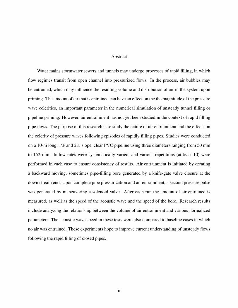
Figure 2.3: Experimental data presented by Mortensen et al. [2011]. The pipe diameters are as fol-lows in (cm); � 7.62, � 17.7, ◦ 30.0, N 59.1. The bold line is the proposed equation by Mortensenet al. [2011] and the other is Kalinske and Robertson [1943]

Mortensen et al. [2011] is presented in Figure 2.3. In a subsequent study, Mortensen et al. [2012]

studied the effect of the location of the hydraulic jump within a closed conduit on air entrainment.

The authors determined that when the jump was too close to the pipe outlet the entrainment was

independent of Fr at the toe of the hydraulic jump. A diagram from the study by Mortensen et al.

[2012] showing the various locations of the hydraulic jumps in his experiments can be seen in

Figure 2.4.

A paper by Skartlien et al. [2012] explained that the volume, or flux of entrained air is caused

by water being ejected from the interface of the hydraulic jump for flows with strong Froude

numbers which are able to generate rollers. The ability of the water to be ejected from the hydraulic

jump is a function of the kinetic energy and cross sectional flow properties of the jump. When the

air is ejected from the interface of the jump it entrains more air when in plunges back into the

free surface flow ahead of the bore. This study sought to investigate the process of air entrainment

within a closed conduit rather than the relationship between inflow properties and entrainment air

demand.

Another experimental study for applications of pipeline priming was conducted by Hou et al.

[2014] exploring the rapid filling of large-scale pipelines. In the work, the authors reported air

12

h

Figure 2.4: The three cases and locations for hydraulic jumps tested by Mortensen et al. [2012] inwhich Lr = length of roller, Lj = length of jump and La = length of aeration.

13

entrapment in rapid filling processes along the advancing water inflow interface. The initial condi-

tions involved a near-empty pipeline (some sag points existed), to which flow was rapidly added.

Air pockets became entrapped behind the leading edge of the filling front. Unlike typical water

transmission mains the experimental apparatus used by Hou et al. [2014] had the only air ventila-

tion point for the pipeline at the downstream end of the system.

An actual pipeline filling study was presented by Vasconcelos et al. [2009], who monitored

the filling of a purified water transmission main in Brasilia, Brazil. Flow rates and pressures were

measured at selected locations along the 4.4-km long, 350-mm ductile iron pipeline. A numeri-

cal model based on the Saint-Venant equation modified by the two-component pressure approach,

developed by Vasconcelos and Wright [2006], was used to compare field measurements with nu-

merical model predictions. While the model predictions agreed well with field measurements,

some discrepancies were attributed to the presence of air that was entrapped during the filling

process.

In summary, past research addressed how air is entrained in stationary hydraulic jumps in a

closed conduits and how air pockets are captured during rapid pipeline filling events. Past research

also investigated how entrapped air interacts with water in a pressurized pipeline as well as the ef-

fects air has on pressure peaks and pressure oscillations. Yet none of the above literature addresses

air entrainment in a backward moving pipe filling bore generated in a pipeline filling event.

14

Chapter 3

Knowledge Gap and Objectives

Upon review of the previous literature, it is proven that the behavior and flow characteristics

of air entrainment in the rapid filling of pipelines via backward-moving pipe filling bores are still

unknown. While other researchers have investigated the creation of air pockets in rapidly filling

pipe conditions and properties of air entrainment through static hydraulic jumps in conduits, none

of these studies implemented the use of a backward pipe filling bore. These past investigations

considered a variety of variables such as slope, Froude number, conduit shape, water temperature

and bore location. Yet none of the closed conduit research with regards to air entrainment via

hydraulic jumps have looked at what happens once the bore is no longer static and instead moves.

The purpose of the present study is to address this knowledge gap through systematic exper-

imental investigations. Such work will involve repetitive experimental testing for a range of pipe

diameters and flow rates for different slopes. The aim is to further study the relationship between

Froude numbers and air entrainment and compare these findings with those of previous researchers

for static bores. In addition to comparisons of air entrainment to Froude number, a variety of other

non dimensional parameters are also compared. It is also an objective to discuss observed mechan-

ics of air entrainment and how this entrained air impacts acoustic wave celerities.

15

Chapter 4

Methodology

4.1 Apparatus Description

The experimental apparatus included a reservoir with a pump that circulated water in a closed

system based on 152.4-mm, 102-mm, and 50.8-mm schedule 40 clear PVC pipes with a length of

10 m. This circulation system has two sides that branch from a T junction in the pipe. One side

is a simple circulation branch that allows continued circulation when the experimental apparatus

branch is shut off. This allowed for the ability to maintain a steady pressure head on the experi-

mental side as well as prevent the pump from overheating during the duration of the experimental

run. On the experimental branch, water flows were passed initially through an upstream knife gate

valve that was used to regulate the amount of flow entering the apparatus. Once the water had

passed the knife gate valve, it flowed through junctions that reduced turbulence. this junction also

maintained the full submersion of a Nortek Vectrino Micro ADV so proper velocity monitoring

was possible. The water would then enter the main reach of clear PVC pipe in which flow became

free surface flow. At the end of the clear PVC reach was a T-junction, in which the main branch

was connected to a second knife gate valve opened to atmosphere. The T-junction derivation led to

a reduction and a fast-acting solenoid valve (initially fully closed) operated upstream with a power

switch. After the knife gate valve at the end of the segment of clear PVC the water would flow into

a reservoir. The water was pumped from the reservoir into a 102 mm drainage port in the wall using

two high head sump pumps. A sketch of the apparatus can be seen in Figure 4.2 as well as a list of

all electrical instruments and components as seen in Table 4.1. A high resolution camera, (1080p),

was also used as part of the experimental set up. This camera was on a tripod that looked at the

upstream section of the clear PVC reach. The functions of the camera in experimental procedure

will be described later.

16

Figure 4.1: A view of the 102 mm configuration looking upstream

Figure 4.2: The apparatus used to run the experiments

17

Instrument/Component Operating LimitationsASCO-8210G004 Solenoid Valve >0.34 Mpa

Nortek Vectrino Micro ADV >0.10 m/sMEGGIT-ENDEVCO 8510B-15 <0.10 MpaMEGGIT-ENDEVCO 8510C-50 <0.34 Mpa

Extech HD750 Manometer <0.34 MpaNational Instruments NI- USB6210 None

Table 4.1: List of the various electrical components used as well as their operational limits.

The PVC pipeline was comprised of 3.3 meter segments connected via rubber couplings. The

clear PVC was mounted to a metallic truss that was supported by metal jack stands. The pipe was

anchored to this truss via elastic cords. The upstream knife gate valve was bolted to a wooden truss

that supported the pipe leading up to the clear PVC reach. At the upstream end of the experimental

branch, on the 45◦elbow that transitions into the clear PVC pipe, is where the air vent valve was

placed. This can be seen in 4.2. This valve is a regular ball valve that was manually operated.

Along the length of the clear PVC pipe were three piezo-resistive pressure transducers (MEGGIT-

ENDEVCO 8510B-15 or 8510C-50) spaced at approximately at 3.3 meter intervals. Two of these

transducers were rated at 0.1 Mpa and the third was rated at 0.34 Mpa, and all sampled at a rate of

1000 Hz. These transducers were connected to a National Instruments NI- USB6210 acquisition

board. The Micro ADV sampled velocities at a rate of 25 Hz. The velocity measurements were

read in real time via the computer interface to which the Micro ADV was connected. Because of

the inaccuracies in measurements of water velocities for the 50 mm apparatus configuration using

the Micro ADV, water velocities were measured using a head discharge relationship for a sudden

expansion using a differential manometer . Further details about the components used for each test

can be seen in Table 4.2.

Pipe Size (mm) Test Type Solenoid Air Valve Dim Vel Measurement50.8 Decompression ASCO-8210G004 12.7 mm Manometer102 Decompression ASCO-8210G004 19.0 mm Micro ADV152.4 Decompression ASCO-8210G004 38.1 mm Micro ADV

Table 4.2: Component sizes for various experimental runs

18

4.2 Experimental Procedure

In order to normalize the results of impacts of entrained air to wave celerity, a baseline acoustic

wave speed had to be measured in cases with no entrained air. This is the acoustic wave in the

pipeline when there is no air present in the conditions of anchoring that the 10-m apparatus was

subjected. To measure this, the following experimental procedure was used

1. For every tested diameter, the pipeline was very slowly primed with the upstream air valve

open. The solenoid valve and the downstream knife gate were valve closed. During this

filling process, care was taken to remove any air that was entrained or stuck on the pipe

walls.

2. Once the pipeline was completely primed, the air valve was shut and the pipeline was pres-

surized.

3. After a steady state conditions were achieved, the transducers were turned on.

4. The solenoid valve was then maneuvered open and generated a low pressure wave in the

system. Elapsed time for the low pressure wave propagation was captured by the transducers.

5. The solenoid valve was closed and steady conditions were again achieved.

6. The procedure above was repeated several times to improve consistency in the baseline re-

sults of acoustic wave speed.

Experimental runs that aimed to create air entrainment through a backward moving pipe filing

bore were conducted with a similar experimental protocol as described below.

1. The experiment started by establishing a steady state in the system in which a target velocity

is attained with minimal fluctuation. Velocity is read in real time using the computer interface

for the ADV.

19

2. The arc length of the area above the free surface in the pipe was measured at regular intervals

along the pipe length. Special attention is paid to ensure that the measurement is taken

normal to the pipe to help mitigate inaccuracies due to parallax and refraction.

3. After this, the three manometers attached to the pipe next to each pressure transducer are

recorded.

4. Prior to rapid filling or initiation of logging sensor data a video camera began recording.

Each step of the process from here on was documented via audio on the camera.

5. Shortly afterwards, the ADV and Transducers were initiated and the experiment proceeded

with the rapid shutting of the knife gate valve which generated a backward moving pipe

filling bore.

6. When this bore reached the upstream end and the flow regime was pressurized, an air valve

that has been venting the air displaced by the backward moving bore is closed.

7. Few seconds afterwards, the opening of the solenoid downstream created a pressure pulse

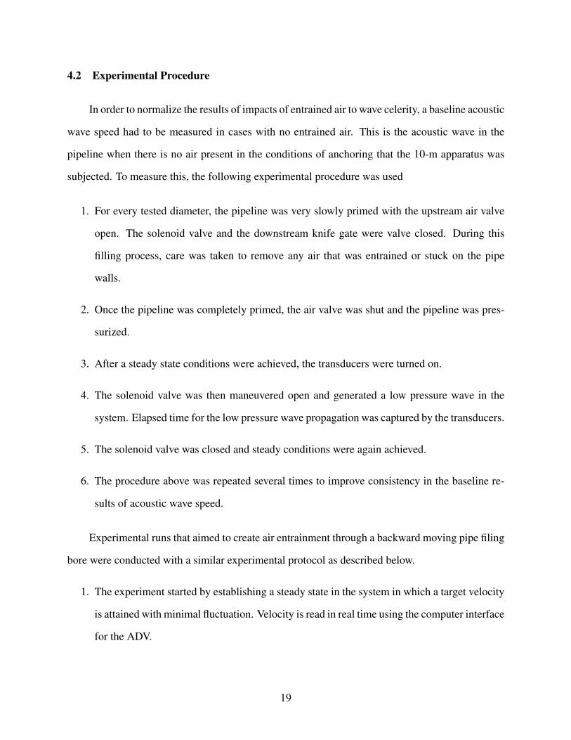
that was captured by the transducers. one of such surges can be seen in Figure 4.4

8. After the solenoid valve closing, MicroADV, pressure transducers, and camera were stopped

few seconds later.

9. The final pressures on the digital manometers was then also read and recorded.

10. Entrained air volume in the pipe is measured, marking the end of an experimental run

The experimental procedure for the down stream valves can be seen in Figure 4.3.

20

Figure 4.3: Shows the valve combination progression repeated for each experimental run. 1.Steady state: Knife gate open, solenoid closed 2. Bore Generation: Knife gate closed, solenoidclosed 3. Pressure wave Generation: Knife gate closed, solenoid open 4. Pressurization: Knifegate closed, solenoid closed.

Figure 4.4: Typical pressure signal used to calculate the acoustic wave speed after being passedthrough a numerical filter.

21

4.3 Data Collection

The pressure transducers results had significant noise in the signal that created some difficul-

ties in detecting the exact point in time at which the acoustic wave had moved over the sensor.

To mitigate this issue, a simple 5-point numerical filter was used to smooth the signals and help

identify more clearly the instant when the peak pressure pulse occurred at each transducer and thus

measure the velocity of the acoustic wave. The same 5 point approach was done with the Micro

ADV measurements to eliminate noise from the recorded velocity data. The numerical filter used

is as follows:

P(i) =15

j=2

∑j=−2

v[i+ j] (4.1)

Where P(i) is the filtered pressure at time i along the signal, and v[i+ j] is the voltage that

was recorded by the transducers at time i+ j.

The air pocket was measured using circular geometry gathered from arc lengths taken at

given intervals. Unfortunately, a small part of the air pocket was hidden from view behind a rubber

gaskets and into a 45-degree elbow made of regular non-transparent PVC pipe at the upstream end.

A sketch of this can be seen in Figure 4.5 An estimated pocket volume for the gasket was taken

based on the closest visible arc length and the length of the gasket plus the length of the PVC lip on

the 45◦coupling. This can also be seen in Figure 4.5. An ellipsoid equation was used to estimate

the amount of air in the elbow of the PVC joint. To dimension this ellipsoid, a measuring tape was

pulled along the projected water surface inside the gasket upstream toward to the back of the 45

degree elbow. Then the total length to back of the elbow minus the length of rubber gasket and

PVC lip was calculated to give an ellipsoid depth. This dimension is also sketched in Figure 4.5.

Using geometric properties, a top width of the water surface was calculated, then the distance from

the water surface to the roof of the pipe were calculated. The volume of the ellipsoid, gasket, and

visible air pocket were summed to determine the total approximate volume of air.

These air volumes were then adjusted to their atmospheric equivalents using the pressure

readings from the manometers at the end of each run. The velocity of the bore at the upstream

22

Figure 4.5: This figure shows how the non-visible portion of the PVC pipe was dimensioned. Thehatched area is the water inside the pipe with the air pocket on top. A tape was projected along thewaters surface to the back of the PVC elbow to determine the ellipsoid depth.

end of the pipe (as it approached the air ventilation point) was measured using a frame by frame

measurement, accurate to 1/30 seconds, from the video camera that recorded the experiment. Also,

the speed of the bore was manually paced using audio queues at 2 foot intervals. Due to high

variability of the air entrainment process the test were carried out in a series of repetitions (at least

10) for at least three different velocities on 1% and 2% slopes. Each of these series were carried

out in each of the three pipe sizes. The velocities varied for the different pipe slopes and pipe

diameters between 0.20 m/s and 0.45 m/s. Flow velocities for the different test were limited by the

desired normalized upper flow rate or the pumping capacity of the laboratory recirculation system.

The limiting factor the the 152 mm pipe diameter tests was the ability to drain the water out of the

reservoir that the system emptied into. The limiting factor for the lower flow rate threshold was

the ability to generate a bore strong enough to entrain air. Table 4.3 presents details for each test

condition considered in this work.

23

Pipe Size (mm) Q* 1% slope Q* 2% slope50.8 0.29, 0.35, 0.46 0.29, 0.40, 0.46, 0.52102 0.16, 0.25, 0.29 0.16, 0.25, 0.33152.4 0.13, 0.20, 0.23 0.17, 0.20, 0.23

Table 4.3: Detailed flow rates for each series of test

4.4 Troubleshooting

Each experimental system was subject to its own challenges and unique mitigating parame-

ters. The following is a record of issues that arose in the lab and how they were mitigated.

Earlier trials were conducted without the use of the circulation branch. This lead to an extra

step in shutting down the pump which lead to a drop in head. This steady drop in head was caused

by the pump ramping down as well as leaks along the length of the apparatus. The only way to

gather manometer data that would be useful was to rapidly read the values out loud so they could

be recorded by the camera immediately after turning off power the pump following the termination

of the data logging by the transducers. Major problems with this approach were the inability to

accurately measure final pressures in the system at both the very end of the run and the pressures

after the air pockets were measured to compute their atmospheric equivalents. The implementation

of the circulation branch mitigated this issue entirely.

The initial set up also included two cameras. The extra camera did not reveal any relevant

information and was instead a hassle. For this reason the one camera alternative was adopted.

Leakage was another issue that required extensive trouble shooting. The first method of at-

taching pipes was to use short wood screws to fasten the pipes to the PVC couplings and then apply

generous amounts of silicone caulking to the outside seam where the PVC pipe slid into the re-

spective coupling. This method was troublesome and resulted in leaking as the caulking was often

blown out of the connections when the system was pressurized. These leaks would suck air into the

system in sub atmospheric conditions that occurred at steady state. This air being sucked into the

system negatively impacted experimental runs by adding unwanted air to the system. The solution

to this issue was to cement various segments of multiple PVC components together with PVC hot

24

weld cement. This in turn created modular units that could be interchanged easily with the rubber

gaskets that connected them. While this worked well for the 102 mm and 50 mm pipe sections,

the cost of 152 mm pipe segments and couplings required a revisit to a non permanent solution for

fastening the pipes. The solution designed in the lab was to use the caulk from the inside of the

coupling rather than the outside. Once the joint was screwed into position, a generous amount of

caulking was applied to the inside lip of the pipe where it sat against inside wall of the coupling.

This method was effective because the water pressure inside the pipe pressed the caulking further

into the seam rather than off the connection.

To ensure that there was no leakage around the air release valve at the upstream end, the

valve was attached by first cutting a circle with a power tool that is slightly smaller than the metal

coupling that was to be used. Then the metal threaded coupling was screwed into the hole so that

the metal threads would thread the hole in the softer PVC plastic. Once the coupling was screwed

in a layer of silicone caulking was applied around the outside. Right after the caulk was applied the

ball valve was screwed onto the coupling and tightened down until the coupling started to screw

further into the pipe wall. The hope was that the wet caulking would be pulled into the connection

between the pipe wall can metal coupling via the couplings threads. This was the most important

seal of all because an air leak around this valve would allow for all the entrained air to seep out of

the system at the end of each experimental repetition.

The earlier repetitions of these experiments involved moving and switching out transducers.

The initial first few test used a .034 Mpa transducer and a .34 Mpa transducer. The .034 Mpa

transducer produced a clear signal that was easy to interpret, however repetitive excessive pressure

peaks from the series of runs eventually damaged this transducer. To make the shuffle of the

transducers more manageable, a USB cord was spliced and the male end was soldered to the

transducer and the female end was attached to the shielded cable. Figure 4.6 shows the pre and

post USB transition for connecting the pressure transducers. These transducers were connected

to the National Instruments NI- USB6210 acquisition board. This method was new to the lab and

allowed for simple swapping and moving of sensors between ports in the pipe. The transducers

25

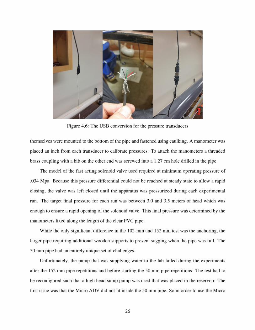
Figure 4.6: The USB conversion for the pressure transducers

themselves were mounted to the bottom of the pipe and fastened using caulking. A manometer was

placed an inch from each transducer to calibrate pressures. To attach the manometers a threaded

brass coupling with a bib on the other end was screwed into a 1.27 cm hole drilled in the pipe.

The model of the fast acting solenoid valve used required at minimum operating pressure of

.034 Mpa. Because this pressure differential could not be reached at steady state to allow a rapid

closing, the valve was left closed until the apparatus was pressurized during each experimental

run. The target final pressure for each run was between 3.0 and 3.5 meters of head which was

enough to ensure a rapid opening of the solenoid valve. This final pressure was determined by the

manometers fixed along the length of the clear PVC pipe.

While the only significant difference in the 102-mm and 152 mm test was the anchoring, the

larger pipe requiring additional wooden supports to prevent sagging when the pipe was full. The

50 mm pipe had an entirely unique set of challenges.

Unfortunately, the pump that was supplying water to the lab failed during the experiments

after the 152 mm pipe repetitions and before starting the 50 mm pipe repetitions. The test had to

be reconfigured such that a high head sump pump was used that was placed in the reservoir. The

first issue was that the Micro ADV did not fit inside the 50 mm pipe. So in order to use the Micro

26

ADV, the 50 mm line coming from the pump had to be expanded into a 102-mm section of pipe

and then reduced again to a 50-mm section. After installing the Micro ADV and running several

tests it became apparent that the velocities in the 102-mm pipe were too turbulent for the Micro

ADV to yield an accurate reading. So a cage was made from metal mesh that was then filled with

marbles. The cage was made to fit snugly in the 102 mm section of pipe and provide head loss that

would in turn reduce turbulence. Although the marble cage was effective in mitigating turbulence,

it was later found that the velocities in the 102 mm section were too low to be accurately read

using the Micro ADV. This being the case, a new method for estimating flow rate in the pipe was

implemented using a head discharge relationship for a pipe expansion. By using a manometer with

two ports on either side of an expansion from 19-mm galvanized coupling to a 38-mm pipe. The

flow was adjusted until a steady pressure differential was reached. Once the system had stabilized,

the flow rate was measured manually using a stop watch a 3 liter container. Each flow rate was

measured 5 times and the average of this series of test was deemed the acceptable flow rate for

the respective pressure differential. Once a series of 5 different pressures and 5 flow rates were

measured, they were plotted to determine a best fit equation that was used for measuring flow rate.

The best fit line had an R2 value of .99. Special attention was paid that the pressures used in the

experiments were within the range of previously measured flow rates.

Anther issue that arose was the surface tension forces that acted on the bubbles entrained in

the 50 mm pipe. Typically for the larger diameter pipes the air bubbles could be coerced upstream

by jostling the pipe. For the 50 mm pipe, a smaller segment of PVC pipe was cut that was about

4 cm long. Then this piece was cut again as to create a semi-circle. A powerful magnet was glued

to semicircle on the concave side. This made for a bubble squeegee that could be moved inside

the pipe wall non invasively with another magnet on the outside. This device worked exceedingly

well. During a repetition the squeegee would be clipped to the crown of the T junction using the

exterior magnet until the repetition was over. The squeegee was small enough that the edges of it

did not dip into the flow at steady state.

27

Table 4.4: Estimated Error of Measurements

Device ± UnitAir Cavity Length 0.5 in.Air Pocket Length 0.125 in.Micro ADV 0.02 m/sTransducer Time Sample 0.001 sManometer 0.3 %Camera 1/30 s

4.5 Error

The Table 4.4 shows the estimated margin of error for each tool used and measurement taken.

The Air Cavity length is the steady state length of the arc along the outer pipe wall that is occupied

by air above the free surface flow. The Air Pocket Length is the length of the outer pipe wall that

is occupied by air that was entrained by the bore.

28

Chapter 5

Results and analysis

There were two observed mechanisms for entraining air mass into the pressurized water flow.

The first was the turbulent interface of the moving pipe-filling bore. The second mechanism ap-

peared to come from the instability in the area-discharge relationship in circular cross sections as

the flow depth approaches the pipe crown. The nature of this entrapment resembled small waves

lapping at the pipe crown. These waves are believed to be similar to those observed by an exper-

imental study conducted by Stahl and Hager [1999]. In that work the irregularities are referred

to as undulations. Because of the similarity of what was observed during experimental repetition

and those observations by Stahl and Hager [1999], air entrained due to the lapping entrainment

mechanism will be referred to as undular entrainment. Considering that the experimental appara-

tus had limitations on the flow rates it could provide, with a maximum Q∗ of 0.25 for the 152-mm

apparatus, most of the cases tested with this diameter had a significant fraction of entrapped air

volume due to undular entrainment. These two mechanisms are sketched in Figure 5.1, along with

the third observed outcome, which was gradual filling with no entrained air volume observable.

Figure 5.1: The three scenarios observed during the experimental testing.

29

This result before described for the 152 mm pipe are consistent with Stahl and Hager [1999].

Stahl and Hager [1999] describes three different types of jumps. The first type is a more gradual

fill with disturbances on the surface associated with Froude numbers less than 1.5. In comparison

with Stahl and Hager [1999], in this thesis gradual filling is defined when the undulations dissipate

before reaching the crown of the pipe. For Froude numbers of 1.5 to 2, Stahl and Hager [1999]

results indicate a similar undular nature of the jump except in this range the waves break at the

upstream side of the jump entraining more air. Stahl and Hager [1999] thus present this range

as the lower Froude limit where small rollers and turbulence in the bore face begin to entrain air.

This exact scenario was also observed in the present experimental study and is described in the

middle sketch in Figure 5.1. Then, for hydraulic jumps with Froude numbers greater than 2, a

bore with rollers at its interface with similar characteristics to those described by Skartlien et al.

[2012] develop. The bore has lost visible undulations and now is predominately characterized by

turbulent rollers and vortices of a classic hydraulic jump. Subsequent depths downstream of the

jump for this scenario were greater than the pipe diameter. The similarities in observed behavior

of hydraulic jumps from Stahl and Hager [1999] study with the present study thus suggest that the

undulation in the static bore observed by Stahl and Hager [1999] is the equivalent of the lapping

mechanism noticed in this present study for a moving bore. It was difficult to ascertain when this

lapping mechanism becomes unimportant, but it is estimated that as the inflow rates become larger

and the Fr ahead of the moving bore increases, the air entrainment through the bore turbulence

should become more dominant.

A final general observation was that the relative size of the bubbles entrained in the 50-mm

apparatus were much larger in comparison to the pipe diameter when compared with the other

pipe diameters tested. This observation is consistent with the study by Chanson and Gualtieri

[2008], in which it is noted that jumps in larger conduits create smaller air bubbles and cause more

entrainment than jumps of similar Froude magnitude in smaller conduits.

30

5.1 Froude Comparison

Differently from Kalinske and Robertson [1943] and Mortensen et al. [2011] studies in which

the location of the hydraulic jump did not change during the experiment, during the filling process

a hydraulic jump moved toward the upstream end of the experiment. Thus, in these experiments

the Froude number of reference was computed in a frame of reference static with respect to the

moving bore, defined as:

Fr =

Qin f lowA f s

+Bvel(g∗ A f s

Twidth

)(1/2)(5.1)

Where A f s is the free surface cross sectional area of the flow ahead of the bore, Bvel is the

velocity of the backward moving bore measured with the camera, Twidth is the top width of the

free surface profile, and g is gravity. The bore velocity term was added to the expression so that

the Froude number was evaluated in a frame of reference that is static with respect to the bore. to

compare the measurements with the regression equation from Kalinske and Robertson [1943] and

Mortensen et al. [2011] studies, air entrained was expressed in terms of a non-dimensional air flow

rate β . Kalinske and Robertson [1943] and Mortensen et al. [2011] measured the air flow rate with

an air flow sensor for a given interval of time. β can be described below as:

β =Vair

T ·Qin f low(5.2)

Where Vair is the total volume of air entrained measured after the priming was completed, T

is the total time that moving bore took to surcharge the pipeline as measured by the audio cues of

the camera, and Qin f low is the water flow rate measured with the Micro ADV or manometer. The

comparison of measured β with the regression equation from previous investigations is presented

in Figure 5.2. Results for 102-mm and 50-mm apparatus and 1% slope agreed well with Mortensen

et al. [2011] expression, but were smaller than Kalinske and Robertson [1943] equation predictions.

Surprisingly, results for smaller Fr values and the 152-mm were above the predictions from both

theoretical expressions. It was noted, however, that in most experiments with this shallower slope

31

Figure 5.2: The Froude number compared with β where β is the air entrained divided be the timerequired for the bore to sweep the system.

32

and 152-mm apparatus the entrainment was characterized by the undular entrainment mechanism

instead of the entrainment through the bore. It is noticed in this chart that even when there was no

identifiable bore (Fr ahead of the bore less than one), the undular entrainment mechanism was still

observable and resulted in a measurable amount of air entrainment along the pipe crown.

Measured β in experiments using 2% pipeline slopes were fairly consistent among the three

tested diameters, albeit all were below the predicted values from Kalinske and Robertson [1943]

and Mortensen et al. [2011] regression equations. In these experiments it was observed that en-

trained air formed pockets that trailed the backward moving bore, however these air pockets in

many cases caught up with the bore interface. When this occurred, the pocket air volume was

released to the air mass ahead of the bore, resembling the occurrence of blow-back phenomenon

described by Falvey [1980]. Such occurrences were also observed in the 1% experiments, albeit

much less significantly since the buoyant forces acting on these pockets were not as intense.

Considering the problem involves a fixed pipeline volume to be primed, it is proposed to study

the normalized entrapped air volume V ∗A is instead of β :

V ∗A =Vair

D3 (5.3)

Where D is the pipe diameter. In general V ∗A results in terms of Froude number reflected

the corresponding values in terms of β for each repetition as shown in Figure 5.3. For the 1%

apparatus, V ∗A increases rapidly for the 50-mm and 102-mm pipelines for Fr values above 1.5.

This is the same class of jump identified by Stahl and Hager [1999] and would correspond the to

scenario where both undular and turbulent air entrainment occur. This dual entrainment perhaps

explains the rapid increase in values for V ∗A . V ∗A results for the 152-mm pipeline were determined

mostly by the lapping mechanism. The results with the 2% slope and larger Fr values were also

consistent among the different diameters, and also showed a dramatic increase in the entrained air

volume for Fr values above 2.

33

These findings are interesting and relevant because it indicates that air entrainment may exist

in fillings even in the absence of pipe-filling bores and strong hydraulic jumps. While in the range

of the tested Fr numbers the overall entrained volume may not be significant, this amount of air is

sufficient to affect the acoustic wave speed in the pressurized regions of the flow, as is described in

subsequent sections. While the instability in the depth-discharge relationship has been recognized

as cause for free surface instabilities as the water depth approaches the pipe crown, there has

been no reported studies measuring the amount of air that can be captured through this undular

entrainment mechanism. Perhaps, Froude is not the best parameter to characterize air entrainment

during rapid filling pipe conditions. For instance, what would be considered a normally sub-critical

flow regime can become critical when taken into considered in moving reference. Such is the case

in image A of Figure 5.5 which is one of the observed repetitions for lapping.

A majority of the experimental repetitions were characterized by air entrainment through

bores with the exception of some conditions involving the 152 mm pipe at 1% slope. One of such

trails can be seen in Figure 5.4. This top image in this figure shows a weak bore as it is passing

in front of the camera. The bottom image in 5.4 is the subsequent depth trailing the bore. It can

be observed that even in the presence of this weaker bore, there are undulations in the free surface

after the bore that are large enough to entrain air. This entrained air is shown in Figure 5.6.

The bores seen in Figure 5.5, are another example of the undular entrainment observed in the

1%, 152 mm diameter test. The top image shows a repetition from the 1% slope and the bottom

shows a repetition from the 2% slope. The normalized flow for the two runs are the same. The top

picture shows a bore thats subsequent depth is slightly less than the crown of the pipe. The front of

the bore seems to end at the second line from the left. The waves in the free surface behind the bore

from the top image touch the crown of the pipe trapping air pockets. The bottom image from the

2% runs shows a stronger bore that fills the entire pipe. This is an example from the 152 mm pipe

test that does not have significant entrainment from the undulating mechanism. Detailed observa-

tion of the video from the different experimental runs reveals similar additional cases where the

subsequent depth was very close to the diameter of the 152 mm pipe. The jump appeared to reach

34

Figure 5.3: Froude number compared with V ∗A for both 1% and 2% slopes. Each point is an averageof repetitions.

35

Figure 5.4: A frame taken from the camera of the case 2 bore seen in the 6 in pipe. The top imageis the bore advancing and the bottom shows after the bore has passed

36

Figure 5.5: Both pipes have the same Q∗, the top image has a 1% slope with Fr. = 1.4 and thebottom image has a 2% slope and Fr. = 2.6

37

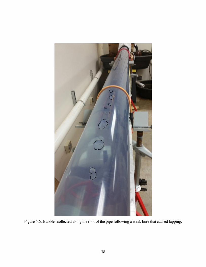
Figure 5.6: Bubbles collected along the roof of the pipe following a weak bore that caused lapping.

38

the crown of the pipe, however, large pockets associated with undulation were still visible before

the standard length of the jump (5-7 times the height of the jump) had passed. The experimental

observations did not provide a clear transition point between undular and turbulent dominated air

entrainment.

An analysis of the behaviors of air pockets in a pipeline leads to three possible behaviors

which have been discussed in previous investigations by authors like Escarameia [2007]; Lauchlan

et al. [2005]; Wisner et al. [1975]; Pozos et al. [2010]. The first is that the air pocket is dominated

by drag forces and is swept downstream, the second is that the pocket does not move due to

dominating surface tension forces, and the third is that buoyant force dominates and the pocket

moves upstream as bubbles merge to create air pockets that resemble gravity currents.

The possibility for air to be swept away via hydraulic clearing is possible for a stationary

hydraulic jump. If the water velocity in the surcharged section of the pipeline is high enough then

the air pockets will be swept away. These minimum velocities are discussed by Escarameia [2007]

and Pozos et al. [2010]. Hydraulic clearing is not possible in this experimental study because the

water velocity behind the moving bore is essentially 0.

In this experimental study it was observed that if the moving bore was weak, the air pockets

along the crown caused by undular entrainment were small and dominated by tension forces. These

air bubbles can be seen in Figure 5.6 after the experimental repetition and pipeline pressurization.

Perhaps, if this equivalent bore occurred in a stationary front, these smaller air pockets would not

be entrained. If a air pocket was formed in by an undulation in a stationary bore, where tension

forces dominated, then the air pocket would not move from its location. As the interface between

the hydraulic jump and the pipe crown oscillated, the air pocket would be simply form and then

dissipate with each oscillation. Perhaps these smaller pockets like the ones seen in Figure 5.6 can

only been entrained by a moving bore.

Based on the observations from this current study, it is possible that water transmission mains

may entrain air via this undulation mechanism in a filling event. Once the undulation bubbles are

entrained by the moving bore, it may be impossible to remove them if tension forces dominate. The

39

suggested equation proposed by Pozos et al. [2010] states that much larger velocities are required

in larger pipes to clear air pockets by hydraulic means. These velocities could be uncommon in

transmission mains. For much larger pipes such as storm water mains, these air pockets are are

more likely to be dominated by buoyant forces and result in a blow back event. This is suggested in

a work by Zukoski [1966] presented by Escarameia [2007] that suggest surface tension and viscus

forces become negligible in pipes with diameters of 175 mm or greater.

Figures 5.7, 5.8, 5.9, and 5.10 show frames taken from the video of the various scenarios that

were run. These images have the pipe diameter, slope, normalized flow rate and Froude number

for each series of test. The undular ripples can be seen clearly for the 152 mm, 1% slope tested in

Figure 5.8.

40

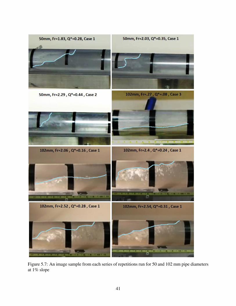
Figure 5.7: An image sample from each series of repetitions run for 50 and 102 mm pipe diametersat 1% slope

41

Figure 5.8: An image sample from each series of repetitions run for the 152 mm pipe diameter at1% slope

42

Figure 5.9: An image sample from each series of repetitions run for 50 and 102 mm pipe diametersat 2% slope

43

Figure 5.10: An image sample from each series of repetitions run for the 152 mm pipe diametersat 1% slope

44

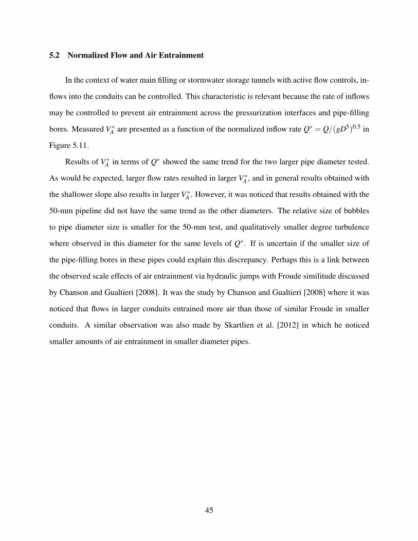
5.2 Normalized Flow and Air Entrainment

In the context of water main filling or stormwater storage tunnels with active flow controls, in-

flows into the conduits can be controlled. This characteristic is relevant because the rate of inflows

may be controlled to prevent air entrainment across the pressurization interfaces and pipe-filling

bores. Measured V ∗A are presented as a function of the normalized inflow rate Q∗ = Q/(gD5)0.5 in

Figure 5.11.

Results of V ∗A in terms of Q∗ showed the same trend for the two larger pipe diameter tested.

As would be expected, larger flow rates resulted in larger V ∗A , and in general results obtained with

the shallower slope also results in larger V ∗A . However, it was noticed that results obtained with the

50-mm pipeline did not have the same trend as the other diameters. The relative size of bubbles

to pipe diameter size is smaller for the 50-mm test, and qualitatively smaller degree turbulence

where observed in this diameter for the same levels of Q∗. If is uncertain if the smaller size of

the pipe-filling bores in these pipes could explain this discrepancy. Perhaps this is a link between

the observed scale effects of air entrainment via hydraulic jumps with Froude similitude discussed

by Chanson and Gualtieri [2008]. It was the study by Chanson and Gualtieri [2008] where it was

noticed that flows in larger conduits entrained more air than those of similar Froude in smaller

conduits. A similar observation was also made by Skartlien et al. [2012] in which he noticed

smaller amounts of air entrainment in smaller diameter pipes.

45

Figure 5.11: The normalized flow rate compared with V ∗A . Each point is an average of repetitions.

5.3 Gravity Currents

As mentioned earlier, it was noted that in some experiments larger air pockets trailing the

backward filling bore would catch up to the bore and escape to the air mass ahead of the bore. In

such conditions, referred to as blow-back, it is hypothesized that the motion of these air pockets

would resemble the motion of discrete air-water cavities, a subject discussed in classic works on or

gravity currents presented by Benjamin [1968]; Baines [1991]; Corcos [1992]. Benjamin [1968]

research pointed that the maximum celerity of such gravity currents in circular pipes would be

limited to 0.54√

gD. Thus, it is further hypothesized that if the bore front has velocity inferior

to this celerity value it would be feasible that the pocket could catch up with the pressurization

interface , leading to the occurrence of blow back during filling events.

Measurements of the bore velocity performed in the experiments were averaged for each

tested conditions and presented along with V ∗A in Figure 5.12. The bores velocity and the cavity

celerity are both normalized by√

gD. In Figure 5.12, the maximum gravity current celerity (“cavity

46

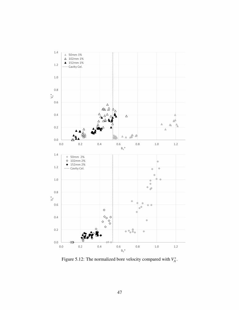
Figure 5.12: The normalized bore velocity compared with V ∗A .

47

cel.”) predicted by Benjamin [1968] is also shown as a vertical line at the horizontal coordinate

0.54.

It is noted that most of the backward moving bores velocities measured with the larger pipe

diameters are below the maximum theoretical gravity current celerity. The bores obtained with

50-mm pipe, and larger inflow rates as well, were consistently above the maximum cavity celerity.

This is consistent with observations in the experiments, in which there was no reported occurrences

of blow back during the filling of 50-mm pipelines. Blow backs occurrences were observed in

experiments involving the two larger diameter pipes, and were more common when the steeper

slope of 2% was used. This is possibly caused by the more pronounced buoyant forces acting on

the entrapped air pockets behind the bore in that slope. Results presented in Figure 5.12 reflect

this observation, since the number of repetitions in which the final V ∗A was above 0.2 were much

fewer for the 2% when compared to the 1% case. Also, blow back occurrences were comparatively

more common in the largest diameter of 152-mm, which is reflected in the fact that there was no

V ∗A values above 0.2 measured for that diameter and the 2% slope.

Other interesting observations yielded by these experiments are estimates of the length of

the bore or pressurization interface L f for all tested cases. The length, measured with the aid of

captured frames by the high definition camcorder, corresponded to the distance from the toe of

the bore to the surcharged interface along the axis parallel to the length of the pipe. The length,

normalized by the pipe diameter is correlated with the flow rate and presented in Figure 5.13.

As it would be anticipated, a larger flow rate will create steeper pressurization interfaces that had

smaller L f /D values, and this trend was observed across all tested diameters. The values L f /D

ranged from less than 1 up to 5, with the range slightly larger for the 2% slope experiments. It

should be noticed that for some of the 1% slope experiments the bore front was so shallow that the

location where it touched the pipe crown was too far back and was not captured in the camera field

of view of approximately 1.0 meter.

48

Figure 5.13: The ratio of the bores interface to diameter of the pipe for both 1% and 2%. Errorbars are show .25D because lengths were estimated

49

Figure 5.14: This figure shows how the parameter L f was estimated. The black tape lines arespaced at 152-mm intervals.

5.4 System Priming Rate

While all of the above terms are good descriptors of data from the experiments, an additional

term, SPR was created to compensate for the ratios of length to diameter as well as the time

that the bore was present in the pipe. Experimental procedures for a static hydraulic jump used

three constant parameters; Froude number, pipe diameter, and a duration of time over which the

experiment was run. In the experiments conducted for this thesis it was not possible to control

the duration of each run. This is because the time taken to fill the pipe was a function of volume

and flow rate. This new parameter, SPR, takes into consideration the geometric properties of the

pipe,the average cross sectional area of the air volume in the free surface profile and the inflow

rate.

SPR =Qin f low

Aair ·L√

D/g (5.4)

Where L is the pipeline length and Aair is the cross sectional area of the pipe that does not

have water when conditions are steady state. This new parameter for normalizing time is shown

in Figure 5.15. The results in Figure 5.15 point that the larger SPR values, associated with faster

pressurization interfaces, are linked to more air entrained. This is consistent with higher flow

50

Figure 5.15: The normalized time compared with V ∗A . Each point is an average of repetitions.

rates to generate stronger Froude numbers and faster bores. Over all, this new parameter seems

to suggest the existence of scale effects of pipe diameter on quantities of air entrainment. These

scale effects can be seen in figure 5.15. The results for both the 2% and 1% slopes seem to follow

a similar trend for the larger diameter pipes. This trend however does not seem to hold true for

the 50 mm values. The 50 mm pipe diameters, however, still appear to entrain similar amounts of

air for a given SPR when compared to the 102 mm and 152 mm diameter pipes with the exception

of the 50 mm 2% slope test at higher SPR values. What is most notable about SPR is the trend

that is identified in Figure 5.15. Results indicate a region of SPR values from 0.003 to 0.005 there

the trend for most of the pipe diameters is more linear. Lower SPR values would be associated

with pipe filling scenarios that likely have the undular entrainment mechanism present as well as

the possibility of blow back from weaker and slower moving bores. The larger diameters have

similar quantities of air entrainment between 0.003 and 0.005. Perhaps this suggest that undular

entrainment is more consistent than turbulent entrainment in the produced quantity of air entrained.

51

Higher SPR values would be linked with turbulent rapidly moving interfaces that would entrain

much more air.

5.5 Acoustic Wave Celerities

As explained, the experiments involved a dual-valve maneuver strategy. The closure of a

larger, knife gate valve triggered the creation of a pipe-filling bore front propagating backward and

entrained air as it swept across the clear PVC pipeline. Once the bore covered the entire pipe length

and the system was pressurized, a fast opening of a solenoid valve at the downstream end created

a second pressure wave which propagated through the pressurized domain with entrained air. This

air was irregularly distributed over the pipe crown with slightly more regular distribution of air in

cases where undular entrainment had occurred. This slightly more regular distribution of air was

also noticed in the 50 mm pipe diameter where it is speculated that surface tension forces hindered

any air bubble movement upstream. Acoustic wave celerity Cmeasured was measured by calculating

the elapsed time for the low pressure wave to be detected in piezo-resistive pressure transducers

that were spaced 9.1-m away. These measurements were compared with the average of 10 baseline

celerity results (Cbaseline) obtained in conditions of very gradual filling where no observable air

entrainment was detected. The normalized acoustic wave celerities results are presented in figure

5.16.

Wylie and Streeter [1993] present an expression for the acoustic wave speed in homogeneous

systems with low air content. This theoretical expression for the celerity Ct is calculated as:

aw =

√(K/ρ)

(1+(K/E)(D/e)(5.5)

where aw is the calculated acoustic wave speed with no air present, e is the pipe wall thickness and

E is the Young Modulus of elasticity of the PVC material. The air-water bulk modulus of elasticity

K and density ρ are calculated in terms of the air and water densities (ρg,ρliq respectively), volumes

of air, water and pipeline system volume (Vg,Vliq and V respectively), and the bulk modulus of

52

Figure 5.16: The normalized acoustic wave celerities compared with V ∗A . This chart also containsthe theoretical values for pipe size and entrainment.

elasticity of air and water (Kg,Kliq respectively), as shown below:

K =Kliq

1+(Vg/V )(Kliq/Kg−1)(5.6)

ρ = ρgVg

V+ρliq

Vliq

V(5.7)

and additional term aair is calculated using the before mentioned equation with K and ρ being

solved for a volume of air present in the pipe as . These calculated acoustic wave speed aair is

then normalized using the calculated acoustic wave speed when no air is present in the pipe. The

equation goes as follows:

Ct =aair

aw(5.8)

In the plot of Figure 5.16 the theoretical expression calculated with equation 5.5 was also

normalized with the baseline results for the acoustic wave speed considering PVC pipes. Analysis

of these results indicate that the celerity values tend to decrease significantly with V ∗A . Values

53

for V ∗A > 0.4 are at least 30% smaller than the baseline results, but more often 40% smaller than

the baseline result. However, the rate of decrease does not follow closely those of the theoretical

Ct , which can be probably explained by the generally uneven distribution of air in the pipe cross

section. Indeed, results for the 50-mm apparatus indicate that in general the measured celerity

significantly smaller than Ct . This is likely due to the more uniform distribution of air in the 50 mm

pipe whereas results with the 152-mm apparatus are generally above Ct . Scatter in the results are

also more pronounced with the larger diameter apparatuses, possibly because of the more irregular

final air bubble distribution observed along the pipe crown. It was also common for experiments

using larger diameters that most of the air entrained volume to be collected into large pockets that

kept moving upstream or already arrived at the upstream end of the apparatus when the pressure

wave associated with the solenoid was generated. While these results point to a clear decrease

in the celerity in pressurized acoustic wave speed in pipes that have entrained air following rapid

filling, more studies are needed to assess this trend for other pipeline configurations and inflow

conditions.

54

Chapter 6

Conclusion

This present work addresses an issue that is still poorly understood, which is the entrainment

of air during the rapid filling of closed conduits through pressurization interfaces. Practical ap-

plications in which this issue is relevant include the priming of transmission mains and the rapid

filling of closed conduits. Entrainment of air through hydraulic jumps in closed conduits has been

previously investigated in closed conduits in conditions where the hydraulic jump does not change

its position during experiments. The problem involving rapid filling of closed conduits results in

moving pressurization interfaces, and it was uncertain to what extent the findings of these previous

studies would be applicable. Moreover, the entrainment of air can have an impact in the acoustic

wave speed of the pressurized region of the flow once the filling is completed. Yet, such impact

has not been investigated to date in the context of the rapid filling of closed conduits and mixed

flow applications.

One interesting finding was that besides the turbulent air entrainment through hydraulic jumps,

the instability of the free surface at as it gradually approached the pipe crown also results in air en-

trainment. Air entrained in this “undular entrainment mechanism” was generally in slightly larger

pockets, but the size of these pockets was still small enough that most of this air remained attached

to the crown after the bore swept through the system. This mechanism was observed particularly in

shallow slopes and larger pipe diameters, indicating that these parameters may influence the type

of mechanism will control air entrainment. Also, these results indicate that air entrainment may

occur in rapid filling conditions even when a pipe-filling bore does not exist. The threshold for the

complete avoidance of air entrainment was not systematically studied in this work, but observa-

tions in the shallow slopes tested indicate that a Q∗ < 0.1 may be required to avoid air entrainment.

.

55

Results of normalized air flow entrainment β for 2% slopes show that the measured air en-

trainment is below the theoretical expressions developed by Kalinske and Robertson [1943] and

Mortensen et al. [2011]. The blow-back episodes were observed during the priming of lines, par-

ticularly for 2% slope, and this may be an explanation for this discrepancy. Results for the 1%

slope and 152-mm diameter were also discrepant, but this is possibly because the undular entrian-

ment mechanism was dominant in generating air entrainment. Results for entrained air volume V ∗A

were generally aligned with the ones expressed in terms of β . As it would be anticipated, V ∗A val-

ues increased with the magnitude of inflow rate, however, there was a discrepancy for the smallest

diameter tested. An expression reflecting the system priming rate also indicated that more gradual

filling yielded smaller V ∗A , an expected result.

Measured wave speed celerity following rapid filling was significantly smaller than the base-

line cases when air bubbles were not entrained. Theoretical expressions relating air volume and

celerity in closed conduits are not accurate in predicting this decrease. This may be explained

because the air-water configuration following rapid filling is not homogeneous as the air pockets

are often spread out along the pipe crown. Nevertheless, because the measured acoustic wave

speed was at least 40%-60% smaller following rapid filling, this effect warrants further investiga-

tion. One can speculate that this impact may be even more significant in less elastic conduits (e.g.

ductile iron, steel or concrete).

It is recommended that future experiments should explore gaps left by this work, such as scale

effects on the entrainment mechanisms, as well a wider range of Froude numbers and pipeline

slopes. It is planned to conduct related investigations involving larger pipe diameters (300-mm)

also in clear PVC. Additional research could explore how these parameters, such as Q∗, Fr, and

SPR, would relate to V ∗A in the presence of an ambient background velocity. This ambient velocity

would be the product of a partial closing of the downstream knife gate valve. Such experiments

would definitely be useful in the context of urban water systems operating in extreme flow condi-

tions toward a better description of these flows using numerical models.

56

Further investigation on the physical properties of the bore should also be pursued. Questions

pertaining to this may include: at what point does entrainment dominated by undulations transition

into entrainment dominated by a hydraulic jump? Is the subsequent depth of the jump in relation

to pipe diameter an indicator of whether or not undular entrainment will occur or rather is it related

to subsequent depth of the different zones of the hydraulic bore? For instance this could be the

depth at which the aeration length or depth at which the length of roller stops. Additionally, future

experiments should be carried out with additional pipe diameters and slope to asses to what extent

the observed mechanisms very with these parameters. In conclusion,while providing insight into a

previously unknown phenomena, this study has also raised other questions that will require further

investigations to be fully addressed.

57

Bibliography

Baines, W. D. (1991). Air cavities as gravity currents on slope. Journal of Hydraulic Engineer-ing, 117(12):1600–1615.

Benjamin, T. (1968). Gravity currents and related phenomena. Journal of Fluid Mechanics,31(2):209–248.

Chanson, H. (1995). Air-water gas transfer at hydraulic jump with partially developed inflow.Water Research, 29(10):2247–2254.

Chanson, H. (2006). Air bubble entrianment in hydraulic jumps, similtude and scale effects.Technical report, University of Queensland, Dept. of Civil Eng.

Chanson, H. and Gualtieri, C. (2008). Similitude and scale effects of air entrainment in hy-draulic jumps. Journal of Hydraulic Research, 46(1):35–44.

Chanson, H. and Murzyn, F. (2008). Froude similitude and scale effects affecting air entrain-ment in hydraulic jumps. World Environmental and Water Resources Congress.

Corcos, G. (1992). Air in Water Pipes: A Manual for Designers of Spring Supplied Gravity-driven Drinking Water Rural Delivery Systems. Aqua Para La Vida.

Escarameia, M. (2007). Investigating hydraulic removal of air from pipelines. Water Manage-ment, (160):25–34.

Estrada, O. P. (2007). Investigations on the effects of entrained air in pipelines. Dissertation,Stuggart University, Stuggart, Gemany.

Falvey, H. T. (1980). Air-water flow in hydraulic structures. Monograph 41, U.S. Dept. of theinterior, Denver, Colorado.

Falvey, H. T. (2011). Air entrapped in gravity pipeline systems. Journal of Hydraulic Research,49(3):394–395.

Gandenberger, W. (1957). Uber die wirtschaftliche und betriebssichere Gestaltung von Fern-wasserleitungen. Oldenbourg.

Gualtieri, C. and Chanson, H. (2007). Experimental analysis of froude number effect on airentrainment in the hydraulic jump. Environmental Fliud Mechanics, 7(3):217–238.

Hager, W. H. and Bremen, R. (1989). Classical hydraulic jump: sequent depths. Journal ofHydraulic Research, 27(5):565–585.

58

Hager, W. H. and Bremen, R. (1990). Classical hydraulic jump: Length of roller. Journal ofHydraulic Research, 28(5):597–628.

Hamam, M. A. and McCorquodale, J. A. (1982). Transient conditions in the transition fromgravity to surcharged sewer flow. Canadian Journal of Civil Engineering, 9(2):189–196.

Hou, Q., Tijsseling, A., Laanearu, J., Annus, I., Koppel, T., Bergant, A., Vuckovic, S., Ander-son, A., and Westende, J. V. (2014). Experimental investigation on rapid filling of a large-scalepipeline. Journal of Hydraulic Engineering, 140(11).

Kalinske, A. A. and Robertson, J. M. (1943). Entrainment of air in flowing water: A symposium:Closed conduit flow. Transactions of the American Society of Civil Engineers, 108(1):1434–1447.

Lauchlan, C., Escarameia, M., May, R., Burrows, R., and Gahan, C. (2005). Air in pipelines. Aliterature review. Report SR, 649.

Mortensen, J., Barfuss, S., and Johnson, M. C. (2011). Scale effects of air entrained by hydraulicjumps within closed conduits. Journal of Hydraulic Research, 49(1):90–95.

Mortensen, J. D., Barfuss, S. L., and Tullis, B. (2012). Effects of hydraulic jump location on airentrainment in closed conduits. Journal of Hydraulic Research, 50(3):298–303.

Pothoff, I. W. M. (2011). Co-current air-water flow in downward sloping pipes. StichtingDeltares.

Pozos, O., Gonzalez, C. A., Giesecke, J., Marx, W., and Rodal, E. A. (2010). Air entrapped ingravity pipeline systems. Journal of hydraulic research, 48(3):338–347.

Rabben, S., Els, H., and Rouve, G. (1983). Investigation on flow aeration at offsets downstreamof high-head control structures. In Proc. 20th IAHR Congress, volume 4, pages 354–360.

Rajaratnam, N. (1962). An experimental study of air entrainment characteristics of a hydraulicjump. Journal of Instn. Eng. India, 42(7):247–273.

Rajaratnam, N. (1967). Hydraulic jumps. Advances in hydroscience, 4:197–280.

Sherma, H. R. (1967). Air-entrainment in high head gated conduits. J. Hydraulics Division,102(11):1629–1646.

Skartlien, R., Julshamn, J., Lawrence, C., and Liu, L. (2012). A gas entrainment model forhydraulic jumps in near horizontal pipes. International Journal of Multiphase Flow, 43:39–55.

Stahl, H. and Hager, W. H. (1999). Hydraulic jump in circular pipes. Canadian Journal of CivilEngineering, 26(3):368–373.

Vasconcelos, J. G., Moraes, J. R. S., and Gebrim, D. V. B. (2009). Field measurements andnumerical modeling of a water pipeline filling events. In Event Proc. 33rd IAHR Congress.Enevt Proc.

59

Vasconcelos, J. G. and Wright, S. J. (2006). Mechanisms for air pocket entrapment in stormwa-ter storage tunnels. In Proceedings of world environmental and water resources congress, Om-aha, Nebraska, Paper, pages 40856–14275.

Wisner, P. E., Kouwen, N., and Mohsen, F. N. (1975). Removal of air from water lines byhydraulic means. Journal of the Hydraulics Division, 101(2):243–257.

Wylie, B. E. and Streeter, V. L. (1993). Fluid transients in systems. Prentice Hall EnglewoodCliffs, NJ.

Zhou, F., Hicks, F. E., and Steffler, P. M. (2002). Observations of air-water interaction in arapidly filling horizontal pipe. J. Hydr. Engrg., 128(6):635–639.

Zukoski, E. (1966). Influence of viscosity, surface tension, and inclination angle on motion oflong bubbles in closed tubes. Journal of Fluid Mechanics, 25(04):821–837.

60