DEVELOPMENT AND CHARACTERIZATION OF AN EMERGENCY COMMUNICATIONS SYSTEM

USING NEAR VERTICAL INCIDENT SKYWAVE ANTENNAS

THESIS

Richard A. Allnutt, Colonel, USAF

AFIT/GE/ENG/02M-32

DEPARTMENT OF THE AIR FORCE AIR UNIVERSITY

AIR FORCE INSTITUTE OF TECHNOLOGY

Wright-Patterson Air Force Base, Ohio

APPROVED FOR PUBLIC RELEASE; DISTRIBUTION UNLIMITED.

Report Documentation Page

Report Date 7 Mar 02

Report Type Final

Dates Covered (from... to) Aug 2000 - Mar 2002

Title and Subtitle Development and Characterization of an EmergencyCommunications System Using Near VerticalIncident Skywave Antennas

Contract Number

Grant Number

Program Element Number

Author(s) Col Richard A. Allnutt, USAF

Project Number

Task Number

Work Unit Number

Performing Organization Name(s) and Address(es) Air Force Institute of Technology Graduate Schoolof Engineering and Management (AFIT/EN) 2950 PStreet, Bldg 640 WPAFB OH 45433-7765

Performing Organization Report Number AFIT/GE/ENG/02M-32

Sponsoring/Monitoring Agency Name(s) and Address(es) AFRL/HEH 2245 Manahan Way, Bldg 29 WPAFBOH 45433-7008

Sponsor/Monitor’s Acronym(s)

Sponsor/Monitor’s Report Number(s)

Distribution/Availability Statement Approved for public release, distribution unlimited

Supplementary Notes The original document contains color images.

Abstract The NVIS system characterized in this work was designed to eliminate skip propagation by optimizing thedesign for contiguous coverage. The NVIS technique involves use of transmission and receiving antennasthat create nearly vertical propagation and continuous coverage from the transmitter to a distance of 200miles. Man portable, very low power transceivers (5 watts maximum) and horizontal dipole antennas fivefeet above the ground are used in an NVIS communication system for this work. The system is designedfor the purpose of supporting communication with emergency workers in areas where othercommunication is difficult. Digital and analog effectiveness are compared at this low power range, and thehuman factors of communication error are described.

Subject Terms : Near Vertical Incidence Skywave, NVIS, Emergency Communications, Human Factors, DigitalCommunications

Report Classification unclassified

Classification of this page unclassified

Classification of Abstract unclassified

Limitation of Abstract UU

Number of Pages 114

The views expressed in this thesis are those of the author and do not reflect the official policy or position of the United States Air Force, Department of Defense, or the U. S. Government.

AFIT/GE/ENG/02M-32

DEVELOPMENT AND CHARACTERIZATION OF AN EMERGENCY COMMUNICATIONS SYSTEM

USING NEAR VERTICAL INCIDENT SKYWAVE ANTENNAS

THESIS

Presented to the Faculty

Department of Electrical and Computer Engineering

Graduate School of Engineering and Management

Air Force Institute of Technology

Air University

Air Education and Training Command

In Partial Fulfillment of the Requirements for the

Degree of Master of Science

Richard A. Allnutt III, BA, MPH, MD

Colonel, USAF

March 2002

APPROVED FOR PUBLIC RELEASE; DISTRIBUTION UNLIMITED

Acknowledgments

I would like to express my sincere appreciation to my fellow engineering students. The

many hours of labor they shared with me taught me much of what it is to be an engineer. Special

thanks go to fellow study group members who taught me calculus again and helped me to plunge

for the first time into the murky waters of differential equations and linear algebra.

To my wife and children who, through love and support, helped me to learn how to study

again, I owe everything – except to again state that I remain a bond-servant of Christ.

To my fellow amateur radio operators, and especially to Mr. Frank Beafore, I can offer

only to continue to learn and share, toward the benefit of the general advancement in amateur

radio experimentation.

To the gentlemen of my thesis committee I owe deep thanks for the hours they spent in

helping me formulate and clarify what I would say in this thesis. Dr. Mike Temple, went beyond

this by helping me to chart a course for the last 18 months of my part-time education.

Research in areas where there is little published literature moves from the impossible to

the possible with the enormous storehouse of information using the Internet. Unfortunately, that

storehouse has an effervescent quality of impermanence to it as well. I have referenced a

number of Internet resources in this document, but only when there was no known bound

reference available. For those who may tread in my footsteps, the chair of my thesis committee

within the Air Force Institute of Technology will maintain a paper copy of the Internet sites.

I would also like to introduce the thesis by noting the information here is useful to the

Electrical Engineering, Medical and Amateur Radio communities. I have tried to write so these

words are readable by all three.

Richard A. Allnutt

iv

Table of Contents Page Acknowledgements............................................................................................……...…… iv List of Figures....................................................................................................……...…… vii List of Abbreviations......................................................................................………...…... xi Abstract.........................................................................................................…………........ xiii I. Introduction......................................................................................………….….... 1-1

Objectives........................................................................................……………..... 1-4 Methods.........................................................................................……...……........ 1-4 Terminology.......................................................................................…………....... 1-5 Equipment............................................................................................……...…….. 1-6 II. Background..........................................................................................…….…….... 2-1 Propagation.........................................................................................……..…....... 2-1 Antennas.........................................................................................……….............. 2-10 Communication Techniques................................................................………......... 2-14 Operations.........................................................................................…….…….......2-16 III. Methodology.......................................................................................………..…... 3-1 Overall Configuration.........................................................................………......... 3-1

Antenna description ...........................….........................................…………….... 3-1 Transceiver description ……..………………………………............…………..... 3-3 Transceiver and computer interface……………………………………………….. 3-4

Antenna models........................…………….......................................………......... 3-5 Quantifiable digital and analog communication techniques……………………… 3-39 Data Collection .......................................................................................….……... 3-44 Mobile site description ……...................................................................…..…….... 3-46 Analysis procedures............................................................................…....……...... 3-52 IV. Results...................................................................................................………….... 4-1

Performance Testing...........................................................................…………......4-1 V. Conclusions and recommendations for further research.......................………....... 5-1 Appendix A. – NEC Input Tables.................................................................…….……....... A-1 Appendix B. – Test Word Lists............................................................................……..…. B-1

v

Appendix C. – NVIS “Pre-Flight” Checklist......................................................………......C-1 Appendix D – Dual Band Antenna Configurations………………………………………... D-1 Bibliography....................................................................................................……….........BIB-1 Vita……………………………………………………………………………………….. VIT-1

vi

List of Figures Figure Page

Figure 1. 40 Meter Vertical – 0.1cm diameter vertical element – Standing Wave Ratio.....................................................................................….......3-7

Figure 2. 40 Meter Vertical – Azimuth Field Strength...........................................….........3-7 Figure 3. 40 Meter Vertical – Elevation Field Strength.........................................….......... 3-8 Figure 4. Horizontal 40 Meter Corner Fed Loop –

33 feet above ground – SWR....................................................................…........... 3-9

Figure 5. Horizontal 40 Meter Corner Fed Loop – 10 feet above ground – SWR...................................................................…............ 3-10 Figure 6. Horizontal 40 Meter Corner Fed Loop –

5 feet above ground – SWR....................................................................…............. 3-10 Figure 7. Horizontal 40 Meter Corner Fed Loop –

33 feet above ground – Azimuth............................................................……........... 3-11 .

Figure 8. Horizontal 40 Meter Corner Fed Loop – 10 feet above ground – Azimuth. ......................................................……............... 3-11

Figure 9. Horizontal 40 Meter Corner Fed Loop – 5 feet above ground – Azimuth. ...........................................................……............ 3-12

Figure 10. Horizontal 40 Meter Corner Fed Loop – 33 feet above ground – Elevation..........................................................…............... 3-13

Figure 11. Horizontal 40 Meter Corner Fed Loop – 10 feet above ground – Elevation. ............................................................….......... 3-13

Figure 12. Horizontal 40 Meter Corner Fed Loop – 5 feet above ground – Elevation................................................................….......... 3-14

Figure 13. 40 Meter Dipole – 33 Feet Above Ground – Standing Wave Ratio.................................................................................….......... 3-15

Figure 14. 40 Meter Dipole – 10Feet Above Ground – Standing Wave Ratio................................................................................…........... 3-15

Figure 15. 40 Meter Dipole – 5 Feet Above Ground – Standing Wave Ratio.................................................................................….......... 3-16

vii

Figure 16. 40-Meter Dipole – 33 Feet Above Ground – Azimuth........................……....... 3-16 Figure 17. 40 Meter Dipole – 10 Feet Above Ground – Azimuth...........................…….... 3-17 Figure 18. 40 Meter Dipole – 5 Feet Above Ground – Azimuth...........................……...... 3-17 Figure 19. 40 Meter Dipole – 33 Feet Above Ground – Elevation.......................……....... 3-18 Figure 20. 40 Meter Dipole – 10 Feet Above Ground – Elevation.......................……....... 3-19 Figure 21. 40 Meter Dipole – 5 Feet Above Ground – Elevation.........................……....... 3-19 Figure 22. 40-80 Meter Crossed Dipole – 33 Feet Above Ground – Standing Wave Ratio..............................................................................................……......3-21 Figure 23. 40-80 Meter Crossed Dipole – 10Feet Above Ground – Standing Wave Ratio..............................................................................................……......3-22 Figure 24. 40-80 Meter Crossed Dipole – 5Feet Above Ground – Standing Wave Ratio...............................................................................................…….....3-22 Figure 25. 40-80 Meter Crossed Dipole – 33 Feet Above Ground – Azimuth.....……...... 3-23 Figure 26. 40-80 Meter Crossed Dipole – 10 Feet Above Ground – Azimuth.......…….... 3-23 Figure 27. 40-80 Meter Crossed Dipole – 5 Feet Above Ground – Azimuth........……..... 3-24 Figure 28. 40-80 Meter Crossed Dipole – 33 Feet – Elevation at 0 degrees Azimuth................................................................................……....3-25 Figure 29. 40-80 Meter Crossed Dipole – 33 Feet – Elevation at 90 degrees Azimuth...........................................................................…….......3-25 Figure 30. 40-80 Meter Crossed Dipole – 10 Feet – Elevation at 0 degrees Azimuth..............................................................................…….....3-26 Figure 31. 40-80 Meter Crossed Dipole – 10 Feet – Elevation at 90 degrees Azimuth..........................................................................……........3-26 Figure 32. 40-80 Meter Crossed Dipole – 5 Feet – Elevation at 0 degrees Azimuth...........................................................................………......3-27 Figure 33. 40-80 Meter Crossed Dipole – 5 Feet – Elevation at 90 degrees Azimuth.........................................................................…….........3-27 Figure 34. 40-80 Meter Loops – 33 Feet Above Ground – Standing Wave Ratio.........................................................................................……...........3-28

viii

Figure 35. 40-80 Meter Loops – 10Feet Above Ground – Standing Wave Ratio...........................................................................................…….........3-28 Figure 36. 40-80 Meter Loops – 5Feet Above Ground – Standing Wave Ratio...........................................................................................……..........3-29 Figure 37. Double Loops – 33 Feet Above Ground – Standing Wave Ratio – 80 M.................................................................................……........3-30 Figure 38. Double Loops – 33 Feet Above Ground – Standing Wave Ratio – 40 M.............................................................................……...........3-30 Figure 39. Double Loop – 33 Feet Above Ground – Azimuth..........................…….......... 3-31 Figure 40. Double Loop – 10 Feet Above Ground – Azimuth..........................…….......... 3-31 Figure 41. Double Loop – 5 Feet Above Ground – Azimuth...............................……....... 3-32 Figure 42. Double Loop – 33 Feet High – Elevation at 135 degrees Azimuth........…….... 3-33 Figure 43. Double Loop – 33 Feet High – Elevation at 225 degrees Azimuth........……... 3-33 Figure 44. Double Loop – 10 Feet High – Elevation at 135 degrees Azimuth......……...... 3-34 Figure 45. Double Loop – 10 Feet High – Elevation at 225 degrees Azimuth........…….... 3-34 Figure 46. Double Loop – 5 Feet High – Elevation at 135 degrees Azimuth.......……….... 3-35 Figure 47. Double Loop – 5 Feet High – Elevation at 225 degrees Azimuth........………... 3-35 Figure 48. 40 Meter Loop at 10 feet with Reflector – Azimuth...........................…….........3-37 Figure 49. 40 Meter Loop at 10 feet with Reflector – Elevation.........................……......... 3-37 Figure 50. 40 Meter Dipole at 10 feet with Reflector – Azimuth......................……........... 3-38 Figure 51. 40 Meter Dipole at 10 feet with Reflector – Elevation..................…….............. 3-38 Figure 52. WS8B Station.............................................................................………............3-47 Figure 53. WS8G Home Station..................................................................……...............3-48 Figure 54. Englewood Reserve Station........................................................……...............3-49 Figure 55. Hueston Woods Station..............................................................……...............3-50 Figure 56. Wright-Patterson Station - Topographic................................………………....3-51

ix

Figure 57. Wright-Patterson Station - Satellite Photo...........................……………......... 3-52 Figure 58. Voice Scores for Each Location - Operator A and B..................…………….... 4-1

Figure 59. Percent of Words Correct for Each Location BPSK....................……………....4-2

Figure 60. Percent of Words Correct for Each Location MFSK..................…………….....4-3

Figure 61. Percent Character Errors – BPSK and MFSK.............................…………….... 4-3

Figure 62. Percent Character Errors – Mode Comparison Overall………………………... 4-4

x

List of Abbreviations AM – Amplitude modulation BBC – British Broadcasting Corporation BPSK – Binary phase shift keying COTS – Commercial off the shelf CW – Continuous wave, i.e. Morse code FEC – Forward error correction FM – Frequency modulation HF – High frequency HT – Handheld transceiver LOS – Line-of-sight M – meter MF – Medium frequency MFSK – M-ary frequency shift keying MFSK16 – COTS MFSK program which includes convolutional encoding and interleaving

MHz – megahertz MUF – Maximum usable frequency NEC – National electromagnetic code NVIS – Near vertical incidence sky wave PSK31 – COTS BPSK program for personal computer PVC – Poly-vinyl chloride RF – Radio frequency SSB – Single side band

xi

SWR – Standing wave ratio

UHF – Ultra high frequency VHF – Very high frequency WS8B – Amateur call sign of Mr. F. Beafore WS8G – Amateur call sign of Dr. R. Allnutt

xii

AFIT/GE/ENG/02M-32 Abstract

Near Vertical Incident Skywave (NVIS) techniques involve physical propagation using

the electromagnetically reflective canopy of ionosphere. HF radio transmission is normally

optimized for distances beyond 1000 miles. However, NVIS techniques optimize

communication from the transmitting station out to 200 miles.

A void exists in communication distances beyond line-of-sight and closer than several

hundred miles. Line-of-sight communications can easily be accomplished with transceivers

operating above 90 MHz. Long distance communication around the globe can be accomplished

with HF radios, however HF communication is frequently disrupted by the peculiar nature of

skip propagation. Skip propagation is the tendency for HF waves to be received in the

immediate vicinity of the transmitter and also received several hundred miles away, but to be

missing (skipping) the interval between. This is the result of optimizing the design of HF

antennas for long distance communication.

The NVIS system characterized in this work was designed to eliminate skip propagation

by optimizing the design for contiguous coverage. The NVIS technique involves use of

transmission and receiving antennas that create nearly vertical propagation and continuous

coverage from the transmitter to a distance of 200 miles.

Man portable, very low power transceivers (5 watts maximum) and horizontal dipole

antennas five feet above the ground are used in an NVIS communication system for this work.

The system is designed for the purpose of supporting communication with emergency workers in

areas where other communication is difficult. Digital and analog effectiveness are compared at

this low power range, and the human factors of communication error are described.

xiii

1-1

DEVELOPMENT AND CHARACTERIZATION OF AN EMERGENCY COMMUNICATIONS SYSTEM USING

NEAR VERTICAL INCIDENT SKYWAVE ANTENNAS

I. Introduction

September 11, 2001 was a watershed date for military men and women in the

United States. The thinking and planning for this thesis had progressed through the

spring and summer of 2001, but with the “Attack on America” in September, the

importance of techniques for emergency communication gained new importance and

interest. This exploration of an unusual and little researched communication technique,

i.e., the use of near vertical incidence skywave (NVIS) propagation, poses immediate

usefulness to a society dependent on technologically advanced communication prone to

sabotage and disruption.

There is a long history of military and commercial aviation use of HF radios.

While military HF applications have diminished, the standard worldwide means of

tracking long, over-water, commercial aircraft flights remains HF communications [9].

In some communities, HF communications is often viewed as an outdated,

difficult, and unreliable mode for communicating. It does have its share of problems,

including fading, dependence on the solar cycle, and a high noise background induced by

atmospherics [30]. However, there are attributes of HF communications which are well

matched to new digital capabilities developed with other purposes in mind, but which can

easily be made to work with HF waves [32, 37].

As mentioned above, the limitations of radio communication involve radiated

power, distance and obstacles. It has been said that the finest transceiver is useless

without a practical and efficient antenna. This is because effective radiated power (ERP)

1-2

depends on an efficient link between transceiver and free space [33]. Antennas for HF

transmission are much the same as antennas used in any other frequency band. Varying

as a function of wavelength, real antennas of a size necessary for efficient HF

transmission normally do not resemble either isotropic or free space models. Dipoles and

their derivatives are the primary practical antennas used for HF frequencies [33].

Looking at the practicalities of trying to maximize long distance communication,

antennas were developed which emphasize radio wave propagation toward at the horizon.

Producing a grazing antenna pattern, often referred to in amateur radio literature as

having a low take-off angle, is best achieved using either a vertical antenna, utilizing a

reflective ground plane to create a virtual dipole, or a horizontal dipole located as far

away from the earth as possible [34].

A side effect of emphasizing long distance communication is the production of

skip propagation. Skip propagation is the tendency for HF waves to be received in the

immediate vicinity of the transmitter (line-of-sight and ground wave) and also received

several hundred miles away, but to miss (skip) the interval between [30].

Near Vertical Incidence Skywave (NVIS) techniques involve a physical

propagation technique using the electromagnetically reflective canopy of the ionosphere

[24]. While all HF communications can reflect from the ionosphere, as well as the

earth’s surface, HF radio transmission is normally optimized for distances beyond 1000

miles [35].

NVIS techniques attempt to optimize communication over ranges of 20 to 200

miles. Instead of radiating most energy from the HF antenna at a grazing angle, the

primary lobe of radiated energy is raised toward the zenith. These techniques are based

on the common use of HF radio waves, but the novel techniques involve using antennas

1-3

optimized for nearly vertical propagation. Instead of aiming for long distance,

contiguous short distance communication is the goal [15, 23].

The NVIS communication techniques purposely attempt to circumvent the

generation of skip propagation, making medium distance communication possible. By

design, the direction of propagation in azimuth and elevation can be selected. The

resulting antenna pattern produces spatial selectivity – enhancing some signals while

rejecting signals on the same frequency whose propagated waves are received from other

directions[1].

Antennas designed to work effectively at long distances direct their energy at a

small grazing angle relative to the earth’s surface. Waves propagating beyond the visual

horizon continue to the ionosphere where a portion of the energy is reflected back toward

the earth [24]. The reflection from the ionosphere’s electrons is quasi optical and away

from the transmitter. An area of skip propagation can be formed between the horizon and

the point where the reflection again reaches the earth [30]. The propagating wave is

actually refracted and dispersed during its interaction with the ionosphere. There is no

physical altitude of actual reflection. Instead, an apparent altitude of reflection can be

calculated which is actually at a greater altitude than the more curved path taken by the

electromagnetic wave during propagation [30].

Conversely, if the antenna is designed to direct its radiation in a solid cone

primarily oriented upward and perpendicular to the earth’s surface, the apparent

reflections are primarily downward. Communications can be maintained beyond the

visual horizon with no area of skip. Such antennas can be used to allow communications

to literally “leap” tall mountains and escape from urban canyons where UHF and VHF

transmissions are absorbed by building materials [15].

1-4

There are complexities in designing of NVIS systems [6], including a host of

issues involving ionospheric reflectivity at different times of day and the sun spot cycle

[24]. Practical antennas need to be considered [9]. The form of communication, analog

versus digital, needs further exploration [35]. It is these details that form the body of this

work.

Objectives

Within this thesis, the described history of NVIS communications leads naturally

to new explorations involving digital techniques. Specifically, an experiment comparing

analog voice communication with two digital techniques is described in detail. Using

simple antennas designed to optimize NVIS communications, an experiment using very

low power HF radios is developed and reported. This experiment allows comparison of

the relative merits of newer digital techniques with the analog NVIS communication

systems developed by the US Army and radio amateurs.

Methods

The Federal Communications Commission sponsors the Amateur Radio Service,

among other reasons, to allow experimentation with communication techniques. The

NVIS experiment conducted as part of this research, takes place within the radio

spectrum available for such an experiment by United States Amateur Radio Operators

[30]. The author is licensed by the FCC as an Amateur Extra class licensee with a call

sign of WS8G. As a partner in these explorations, another radio amateur, Mr. Frank

Beafore, WS8B acted as the station control operator of a second station for the

experimental work. Transmissions were made at very low power (5 watts) and from

different locations purposely chosen for their difficult terrain obstacles. Throughout the

1-5

research, data was collected with the expectation of reaching a conclusion regarding the

practicality of the digital modes, as presently available, with analog voice

communication by an experienced radio operator.

Terminology

Certain specialized terms are important to the understanding of these concepts.

As already described, Near Vertical Incident Skywave (NVIS) antennas are used.

Technically, an NVIS antenna has a far field radiation pattern that is directed primarily in

a cone normal to the earth’s surface. Practical NVIS antennas have an antenna pattern

which if visible would look much like a rather tall puffball mushroom [9].

Dipole antennas are used extensively in this research. Normally, they are half

wavelength dipoles implemented as physical wires horizontally oriented. The wires are

connected to the transceiver via 50-ohm coaxial cable and are unbalanced wire antennas

pruned to have a minimum Standing Wave Ratio (SWR) for a specific frequency.

Occasionally, crossed dipole or loop antennas are introduced, both of which are also be

horizontally oriented [33, 34, 35].

Analog communications refers to voice communication using standard single side

band (SSB) techniques on the lower side band of the frequencies considered here [34].

Two types of digital communications are considered. Binary phase shift keyed (BPSK)

transmissions using a published protocol known as PSK31 uses a frequency band about

30 Hz wide. A personal computer program generates the signal [12, 25]. Using another

program, 16-Ary multiple frequency shift keying (MFSK) with convolutional

coding/decoding and interleaving, is tested with a protocol known as MFSK16 [10, 19,

20].

1-6

Equipment

To the maximum extent possible, commercial-off-the-shelf (COTS) materials and

equipment are used in this work. The HF radios were manufactured and certified for

amateur radio use by Yaesu and are designated the FT-817. Operating on 9 to 12 volts

with either an internal battery or external battery, the units are capable of transmitting at

several power levels between 0.5 and 5 watts [13].

All communications were accomplished on the 40-meter (7.000 to 7.230 MHz)

amateur radio bands. More than one band needs to be available to deal with cyclic

changes in propagation. Operator experience (and the application of several rules of

thumb) leads to making the proper frequency choice [30]. Voice communications were

made via the lower sideband using standard single sideband techniques [33]. Digital

signals were created by an interface with a personal computer. The personal computer

ran freeware versions of PSK31 and MFSK16 programs available over the internet. The

computer program for the selected digital mode drives the computer’s standard sound

card (Soundblaster 16) to create (or analyze in receive mode) the audio frequency

signal. The audio signal interfaces the microphone and headphone jacks of the radio.

The communication link was half-duplex; i.e. the radio was either in receive or transmit

mode at any time [11].

To make comparisons between the different modes, a set of standard words was

used to determine the ability to receive with accuracy. This set of words is developed

from the audiology literature and from the aviation medicine practice [31]. It is used by

flight surgeons to determine a pilot’s performance in understanding aircraft radio

communication. Several similar lists are used with order effects controlled. The same

lists were used for the spoken audio (analog) and for the digital modes. In each case, the

1-7

receiving radio operator chooses between similar sounding (reading) words using a

multiple choice score sheet. In addition, for the digital words, a raw score of character

errors was calculated from a direct comparison of the ASCII transcripts of the digital

mode sessions [31].

The antennas used for this research are dipole antennas incrementally designed by

the author using commercial antenna modeling software [28]. Derivatives of the very

simple half wavelength dipole antenna, they have been primarily modified by being

placed close to the ground. During the incremental design process, the goal was finding a

balance between take-off angle and radiated power could be made by adjusting the height

of the dipole above the ground. To decrease the effect of ground wave and multipath

canceling, the antenna was designed to minimize ground wave at some expense of total

radiated signal strength [1].

2-1

II. Background

Propagation

NVIS propagation can be described as a new way of thinking about an old

subject. Radio engineers have been using NVIS techniques for many years, though much

of their work has been directed toward ways of decreasing NVIS propagation.

Early in the history of radio, professionals and amateurs learned methods of

promoting over-the-horizon propagation of HF radio waves. A low take-off angle in the

antenna used by the transmitter and receiver promoted long distance communication.

The means of this long distance communication was gradually understood to be

ionospheric reflection of the HF radio waves [33].

The use of electromagnetic waves for communication parallels development of

science in the western world [17]. Beginning with spark gap transceivers and continuous

wave transmitters, communication techniques progressed to amplitude modulation,

suppressed carrier, frequency modulation, and digital communication techniques. The

communication efficiency is dependent on distance, radiated power, and obstacles

between transmitter and receiver [35].

Frequencies used for communication literally span the spectrum from audio to

light [17]. Early commercial analog communications were conducted at what is now

called the medium frequency (MF) band – commonly known as the AM radio spectrum.

Commercial broadcasters encouraged the government to allocate the high frequency (HF)

spectrum above MF to amateur experimentation, believing these frequencies were

essentially worthless for commercial use. World War II brought military development

and use of higher frequency bands for communication. Introduction of the klystron tube

2-2

made high power transmission above 100 MHz practical. Practical use of Very High

Frequency (VHF), Ultra High Frequency (UHF), and other bands used early for radar and

later for communication was a byproduct of military development [30].

Electromagnetic waves essentially propagate along straight paths. Like light, they

propagate until they are absorbed, reflected, or refracted. The consequential limitation of

line-of-sight (LOS) communications becomes apparent as an uninterrupted line of sight is

lost. Many children have played with handheld transceivers (HTs) and experienced one

of the most discouraging limitations of these HTs, namely, the loss of signal occurring

very soon after one user loses visual sight of the other. The primary limitations of low,

fixed power transceivers is the same as all transmitters- radiated power, distance, and

obstacles. But when one goes around the school building, the primary limitation

becomes the obstacle. If the obstacle is too dense, or contains much metal, the signal is

lost [1].

One way to limit the problems of LOS communication is to put one or both users

at an elevated location, i.e., put one user on top of a hill or tall building. Such a simple

maneuver can extend the maximum effective range of HTs from less than a mile to many

miles. As elevation eliminates LOS obstacles, the range limitation becomes a function of

the radiated power [35].

Line-of-sight communications can easily be accomplished with transceivers

operating above 90 MHz. This includes everything from commercial FM radio to VHF

and UHF. VHF, and later UHF, transceivers were developed during WWII for the

military, but are now ubiquitous in amateur, business, and personal communications [35].

2-3

Similar, but not identical, to LOS communication is ground wave propagation.

Classic experiments have shown that light, and by extension, radio waves diffract around

corners. The amount of energy diffracting around a corner is dependent on the physical

nature of the corner and the radio wave. Different materials, different shapes and

different wavelengths all impact the actual behavior of the diffraction. Over the varieties

of undefined terrain surrounding a radio user, it is clear that energy propagates around

corners that one can not see around. The corner may be a gentle hill, an ocean wave, or

for a short distance, the nautical horizon. Whatever the physical nature of the corner,

this kind of communication link can be thought to be primarily ground wave

communication [35].

The usefulness of ground wave propagation increases with wavelength. VHF and

UHF have very little ability to bend around hills and buildings. One very nice property

of MF transmission is the extent to which the waves can propagate along the ground. It is

this specific property that made MF AM signals, a commercial broadcaster’s dream. A

reasonably high antenna and relatively high power can be used to reach a very large

audience, well beyond the LOS region. The clear channel voices of the major cities can

still be heard well beyond the nautical horizon [34].

The early MF commercial broadcasters did not recognize the potential for sky

wave communication. Giving the short wave frequency bands to amateurs, many of them

thought the HF bands would always be useless. Prone to large amounts of static

interference from atmospheric lightning discharges occurring hundreds (or thousands) of

miles away, the potential to use the HF bands for communication was strongly discounted

[30].

2-4

The long distance properties of HF radio waves begin with the earth’s ionosphere.

Starting at an altitude of about 40 km, and stretching to several earth radii, the ionosphere

is a charged region consisting of ionized particles stripped of their electrons by solar

radiation. The ionosphere is a region of low winds, high temperature (with almost no gas

mass to transmit that temperature to solids) and very low pressure. Depending on the

time of day, season, and the amount of solar radiation, it forms layers (primarily

electrons) which reflect HF radio waves [24].

Amateur radio operators, given the HF bands for experimentation, soon found that

long distance communication around the globe could be accomplished with HF radios.

Between 3 and 30 MHz, intercontinental communication is often practical at reasonably

low power levels[30].

The founding experiments of long distance radio communication were focused on

communication with ships at sea and with intercontinental radio. The primary official

focus was on communication with ships, as there were legal disputes between those who

wanted to use radio waves to communicate between North America and Europe and those

who had paid to lay intercontinental wire on the floor of the Atlantic Ocean [30].

Successful long distance communication requires choice of appropriate

frequencies to exploit the radio reflective canopy of the ionosphere [24]. Medium

frequency waves, such as those used by commercial AM radio transmitters in the

frequency range 0.5 to 1.5 MHz are of most use as direct LOS and extended ground wave

communications. At very high power, and especially at the higher end of the spectrum,

these waves can be heard between cities several hundred miles apart. In the 1930s, a set

of clear channel voice radio stations with power levels of up to 500,000 watts were used

2-5

by commercial radio broadcasters [33]. The author’s father remembers hearing AM

signals from WLW in Cincinnati (500,000 watts) detected by bedsprings in New Orleans,

Louisiana. In the 1930s, lying in bed in the quiet of the night, familiar radio stars could

be heard coming from the metallic springs under the mattress! On a somber note,

medical anecdotes of people being hospitalized in psychiatric hospitals for schizophrenia

(voices in their head) were later found to have actual voices emanating from dental

fillings acting as AM radio detectors. (Always ask someone who hears voices if they also

hear music or radio station call signs.) Later, the clear channel voices of New York,

Chicago, Cincinnati, and Los Angeles were limited to 50,000 watts and reports of

incidental AM detection decreased [33].

Very short waves are also of limited use for long distance communication on

earth [30]. VHF and UHF (and higher) frequencies are of most use in line of sight

communication. They penetrate the ionosphere easily and are used in extraordinarily

long distance communication between earth and far-flung satellites at interplanetary

distances [7]. But on earth, these signals are normally stopped by the first thick physical

horizon made of rock, dirt, or metal [1]. Within these ranges, lower frequency signals are

able to penetrate man made (non metallic) structures, while at the upper ranges, even

household building materials become a significant barrier to radio waves. At the lower

end, the ionosphere can occasionally reflect signals near 50 MHz. Signals near 150 MHz

can occasionally be propagated well over the horizon by tropospheric ducting

(atmospheric wave guide) or briefly by ion scatter created by meteorites. But at the

higher end, 400 MHz into the low GHz ranges, physical objects become more and more

opaque and reflective of radio waves. For these reasons, most use of these waves is line-

2-6

of-sight. Portable communications in these frequencies often assume the form of

handheld transceivers (HTs and cell phones) of very low power output in the range of

less than 10 watts [30].

Ground level VHF, UHF, and microwave communications between handheld

devices is inherently limited to distances of only several miles [34]. These distances can

be extended indefinitely with the use of high towers and dedicated radio repeaters [34].

Amateurs, business band users, and cell phone companies all use this repeater concept to

add range to what is an essentially short-range method of communication. Aircraft based

VHF and UHF communications can be of long distance because the physical horizon is at

a great distance when the aircraft is at cruising altitude. For specialized operations,

repeaters can be aircraft or spacecraft based, allowing long distance communication at the

expense of keeping the aerospace vehicle off the ground and overhead [7].

Between the upper frequencies of medium wave AM and the lower edge of VHF,

there is possibility of reflection of radio waves off the high altitude ionosphere. The

ionosphere begins at 40 km and extends to several earth radii of altitude. The ionosphere

was first described by experimental soundings at a group of worldwide locations. It has

been shown that the reflective planes of mainly electrons change their altitude and

characteristics on both a daily and seasonal basis. Solar events also affect the

characteristics of the ionosphere. The ionosphere is essentially the product of the

interaction of the gasses of the atmosphere with high-energy particles and

electromagnetic waves created by the sun. Thus, most events that change the solar

radiation of the earth change the ionosphere. These changes have profound effect on

ionospheric reflection of radio waves [24].

2-7

Changes in the ionospheric conditions and the condition of solar radiation are

known as space weather. Space weather changes much like earth weather. There are

episodic storms each of which is not open to direct prediction. There are also a number

of cyclic changes that can directly be predicted in time if not in extent [30].

The daily shift from day to night dramatically changes the condition and altitude

of radio reflective layers of the ionosphere. As the day dawns, energy from sunlight

changes the ionosphere so that the Maximum Usable Frequency (MUF) rises. The shift

of seasons likewise brings changes to the ionosphere. The increased length of the day

and greater angle of incidence of sunlight on the ionosphere leads to a higher MUF

[24,30].

The 11 year solar sunspot cycle, recorded for the last several hundred years, also

contributes dramatically to the activity of the ionosphere, with elevated sun spot numbers

leading to a higher MUF and generally better conditions for HF reflection [24, 30].

These space weather phenomena are subject to some prediction or at least the

application of several rules of thumb. An HF radio operator on a commercial airliner

knows that lower frequencies will work better at night and early in the morning. Higher

frequency bands will be more useful as the morning ends and through the evening.

Summer months allow the use of higher HF frequencies in either the northern or southern

hemisphere when contacts are made within the hemisphere. Spring and fall are the

seasons of choice for long distance communication across the equator. Radio amateurs

follow with great anticipation the development of each sunspot cycle as radio propagation

steadily improves in the first half of a cycle and then wanes in the nadir of the cycle

[[30].

2-8

Sunspots make their own individual contribution to HF radio conditions as

markers of specific solar events. A visible group of sunspots (visible about 8 minutes

after they appear - given the distance of the sun from the earth and the speed of light)

may lead to a particle event several days later that has its own independent effect on HF

radio propagation through interaction with the earth’s magnetosphere [24]. During

intense magnetic storm conditions, HF radio communication that relies on reflection from

the ionsophere may be entirely shut down for several hours. The same magnetic storm

may cause considerable damage to orbiting satellites and health risks for astronauts

outside the protective lower levels of the magnetosphere [7].

By the 1940s, the transatlantic radio service was well established and ship-to-

shore communication had been expanded to include communication with intercontinental

air service [34]. Commercial and government short wave radio stations around the world

have heavily depended on high frequency communication. Such broadcasts never gained

the following in the United States that they did in other countries. Nevertheless, the US

has many faithful followers of the BBC Worldwide Broadcasting Network [30].

Part of the attraction of the short-wave broadcasts is their availability at great

distance. This distance was achieved by the propagation methods alluded to previously.

Essentially, they depend on skip to get their message over the horizon [35].

All of which led to a study of skip and improved scientific understanding of the

propagation method. Informally, skip is the tendency of HF radio waves to be heard

well at great distance while they cannot be received at an intermediate distance [30].

2-9

There are two factors that lead to the skip phenomenon. The first is the direction

the transmitting and receiving antennas have their main beams pointed. The second may

involve optical principles that approach total internal reflection [1].

As briefly stated earlier, early emphasis in HF radio was in promoting long

distance communication. There were other communication forms that would work for

short distance. The domain of the HF radio engineer was working out communication

between distant outposts [35].

A study of propagation with ionospheric reflection at close range requires

consideration of the interaction of sky wave and ground wave signals. For the moment,

ground wave signals will be those line of sight electromagnetic waves and those ground

wave refracted waves that come to nearby site. This leads to a combination of waves

observed line of sight and a bit beyond the visual horizon. HF waves have a tendency to

propagate over some hills and small obstructions precisely because they are of long

wavelength [24].

In distinction to these ground wave signals, sky wave signals will be those that are

received after being reflected off the ionosphere. In NVIS work, the direction of

incidence of the incoming HF signal is from nearly vertical [9].

Assuming one can bounce a signal off the ionosphere and a station can receive it

several miles distant from the transmitting station, it is possible for the ground wave to

block the sky wave by destructive interference [24]. A similar situation exists in VHF

and UHF transmissions when signals reflected by structures or delayed by atmospheric

events may arrive in phase or out of phase. Often, moving several inches can

dramatically affect reception of UHF signals. In mobile service, such reception is

2-10

sometimes called “picket fencing” because the audio wave received sounds like it is

received through a picket fence along the road [30]. Similar effects can cause large

changes in cell telephone service well within the expected service range from a transmit

site [32].

Such destructive interference can exist when sky wave and ground wave signals

arrive slightly out of phase. If it is desired to make use of the sky wave signal to be able

to talk over a mountain, into an urban canyon, or to a station 60 miles away, then the

antenna design will need to optimize the sky wave signal while working to keep the

ground wave signal at a minimum.

The problem with communications based on skip is the transience of

communication due to time dependent ionospheric changes. Especially irritating is the

inability of hearing stations just over the horizon to a couple hundred miles away [34].

Antennas

Part of the beauty and the headache of antennas used for HF radio work is their

size. In an era when electrical engineering design is primarily design of chips or the

programming of them, antenna design deals with larger components. These components,

the radiating elements and transmission lines, are of such a size that one can hold them in

a hand and move them easily. The other enjoyable aspect of antenna design is that

experiments can take on an aspect of art where creativity still plays a part [30].

The antennas used for HF transmission and reception (equivalent functions for

design) can be elegantly simple. Horizontal half wave dipole antennas have been used

for a century. Their equivalent, the quarter wave vertical, is also well described,

understood, and widely used [33].

2-11

In amateur radio work, commercially available transmitters are almost always

designed to expect 50-ohms of impedance at the feed point. The 50-ohm coaxial,

shielded cable is the nearly universal transmission line between the transceiver and the

antenna. This is reasonable, if properly pruned dipoles or verticals are the antenna

system. A minimum Standing Wave Ratio (SWR) near 1.2 to 1.4 can be achieved

reducing transmission line heating and loss of power. This SWR is possible because the

natural impedance of the free space dipole is 68 ohms and the natural impedance of the

quarter wave vertical over a perfect conductor is half of that at 34 ohms [30].

The analytic representation of a horizontal dipole antenna has previously been

characterized. The direct component of the horizontal dipole has an electric field θE as

shown here:

≈−

θ

θπ

πηθ sin

cos2

cos

2 r

eIjE

jkrO

where OI is the current maximum,

η is the intrinsic impedance of the medium, r is the distance from the antenna, and

θ is the angel of observation from the y axis (zenith.) The antenna pattern of a horizontal dipole is a well-described doughnut with

minima along the axis of the antenna. Nearer the ground, the pattern becomes more and

more distorted by reflection and coupling, until a greatly diminished hemispherical

pattern exists as the dipole is brought very close to the ground [1].

Because of the physical size of the quarter wave elements, other methods have

been used to reduce the real estate required for the antenna. Elements can be shortened

by adding inductors in the mid span of the antenna or capacitance hats at the distal ends

2-12

of the antenna. These maneuvers have two undesirable consequences. They decrease the

efficient bandwidth of the antenna by affecting its Q and reduce the radiation efficiency

of the antenna [33]. Another approach can be used to decrease the size of the antenna: A

square loop can be employed, decreasing the longest dimension of the antenna by 30

percent [1].

If the troublesome aspects of skip are partly the result of designing antennas to

produce a grazing angle near the horizon, then designing antennas to have a high take-off

angle may be one method to reduce the impact of skip. If the take-off angle can be

modified to be more nearly vertical, then energy with the potential of reflection off the

ionosphere will arrive with the angle necessary to communicate at close range. Skip will

have been eliminated by the simple expedient of not putting anyone within two hundred

miles in a skip zone [9].

With care in the design of HF antennas, certain trade-offs can be made between

generation of sky wave and ground wave energy. A very low horizontal antenna will

have almost all of its energy directed upwards and very little will be transmitted via

ground wave. Unfortunately, severe restriction on the generation of ground wave carries

the price of absorption of a considerable fraction of the output power by the ground,

which may be as close as a fiftieth of a wavelength above the ground [22].

Because of the absorption of power by the ground in NVIS systems, most

operators have used transmitters at or above 100 watts. There is no prior experience in

the literature showing low power NVIS to be practical [16].

Thought has been applied to the concept of using directional antennas or arrays to

point more of the signal upward. Reflectors behind a dipole have been used to increase

2-13

the signal upward. Unfortunately, to be effective, the reflector needs to be back from the

active driven element by something near a quarter wavelength to be effective [1]. Any

antenna of this height produces considerable ground wave [6]. For these reasons, no

attempt to use finite element analysis models of these arrays was attempted.

Certain practical considerations for a mobile communication system were

considered for this system. As discussed in the propagation section, at least two

frequency bands need to be available to contend with the state of the ionosphere daytime

vs. nighttime [9]. In addition, the same frequency spread will help deal with the annual

and 11-year cycles. In the case of the experiments undertaken, the 40 and 80-meter

amateur radio bands were chosen. For operational use, frequencies reserved for the

military in this part of the spectrum could be just as effectively used [9].

For ease and the sake of simplicity, designs were sought which could use a

common transmission line, yet be tuned for use on the two bands. By proactively

designing the antenna system for two frequency bands, all question of interaction

between antenna systems is resolved. In addition, the radio operator need not change

antenna connections when changing frequencies [30].

The intent of this emergency communication system is to be transportable.

Changes could be made in the antenna system to allow mobile use, but the antennas

would consequently suffer a loss of efficiency as they were made physically short with

the use of inductors or capacitors [14].

While transportable, the goal in selecting designs was to work toward the lightest

and least complicated designs available. This approach leads to a design that a single

individual can carry and erect in a few minutes.

2-14

The actual design of the antenna system and the analysis of antenna patterns is

contained in the Methods section of this work.

Communication Techniques

Part of the goal of the experimental approach to this topic is to use lightweight,

minimal power equipment. The transceiver selected, with internal battery supply, has a

maximum output of 5 watts peak power. It is adjustable by steps down to 0.5 watts [13].

In this power range, at distances or in geographic areas that require ionospheric

communication, the received signal will be weak. Successful communication in the

presence of very weak signals can be aided by skilled operators and by the use of digital

encoding procedures [32].

For the purposes of emergency communication, an assumption will be made that

the signals need to be sent and interpreted in real time. A number of digital techniques

can be used to store and forward information with delay. Certain trade-offs can be made

between transmitted power and loss of the ability to interpret a signal in real time. A

well-known example of these techniques is used by interplanetary space probes. Very

detailed digital images can be collected by a distant spacecraft in rapid order. However,

the digital transmission of those images, pixel by pixel, even when compressed, may take

many hours or days with redundant error correction techniques [32].

In the case of real-time or near-real time transmission, communications explored

here are analog speech signals interpreted by a skilled operator, and digital signals

interpreted by an operator.

2-15

Digital signals can be of several types. Binary signals can represent the required

bit stream by operating on the amplitude, frequency, phase, or several combinations of

the transmitted signal [32].

A primitive example of on/off amplitude shifting is continuous wave (CW)

signals sent by hand using the Morse Code. Historically, transient spark gap Morse Code

signals were the first radio signals sent from one point to another. However, very soon

CW Morse signals were being exchanged between distant stations [30].

Binary Phase shift keying (BPSK) was developed for use by spacecraft outside

earth orbit. With BPSK, the phase of the signal is abruptly modified . The bandwidth of

the signal is directly related to the time domain bit rate driven phase shifts. As the bit

rate increases so does the bandwidth required for the signal. Of course, the inverse is also

true. As the bit rate is decreased, the necessary bandwidth decreases [32].

One popular digital communication program (PSK31) has aimed for the minimum

bandwidth to keep up with typing ASCII characters at up to 50 words per minute. Using

a computer sound card to both process the received signal and to generate an audio signal

for the transmitter, the transmitted signal is compressed into a 31 hertz. This leads to

very effective utilization of the small amount of bandwidth available for experimental use

[12, 25].

Other modulation techniques are also available. There are schemes that modulate

multiple levels of phase, amplitude, and frequency [11]. One attractive system available

for evaluation via the use of computer sound cards employs 16 levels of frequency

shifting with convolutional encoding and interleaving [19, 20].

2-16

Much is made in the digital communication literature of bit error rate. Bit error

rates for various communication techniques can be calculated both on an expected basis

and in real time. Bit errors normally roll up into character errors when text is the output

of the communication system. These character errors are subject to correction by

algorithm and by the skilled user [32].

Encoding a digital signal can allow for error correction by retransmission and also

by the techniques of forward error correction (FEC). A number of FEC systems are in

use, but the convolutional encoding scheme of Viturbi is a well-described method of

correcting the errors that may have been received in the communication system. One

COTS program available to the amateur community based on these conditions is

MFSK16 [10].

Operations

Much of the over the horizon military communication requirement and emergency

communication implementation now depend on the availability of high cost

infrastructure. Commercial cell telephone coverage requires a large number of cell

telephone towers. These communication nodes are weak points and are distributed

widely enough as to make them possible targets for anyone desiring disruption of our

emergency response capability [34].

Cell telephone sites are often redundant, with users able to access more than one

site [31]. This is good when a small number of users need access over a wide area.

However, without a priority access system, a local tragedy can bring the system to its

knees. Trunking systems are also prone to failure, just like the cell telephone system,

2-17

when large numbers of users simultaneously try to access the communication system

[32].

Communications are sometimes necessary in emergency operations where no

established repeaters are available. The needs of users can be met with aircraft mounted

or space based repeaters, but at great cost. This may be feasible over the short term, but

becomes less and less attractive for long term communications with rescue or aircraft

accident investigation personnel [7].

An aircraft accident investigation team, a hundred miles from a base in an area,

and not served by cell telephone service (desert canyons) will have a rough go at

communicating with the local military command structure. Aircraft can be used as

temporary repeater sites, but become expensive when an investigation lasts more than a

few days [34].

A very practical solution to these problems is the use of close-in HF

communication with NVIS antennas. Such radio systems with their antennas can be

carried by a single individual in a backpack and with solar cell recharging of their

batteries can be used indefinitely away from any power grid [8, 9].

There is scant literature on the use of NVIS systems for military operations [9].

Unfortunately, the work that does exist is anecdotal and contains little useful research to

allow a planner to understand the engineering concerns or the actual performance of the

system [27].

Emergency communication centers using NVIS antennas can be situated in

valleys or alleys off the high ground. Long cable runs or the necessity of removing the

2-18

communication center from the actual area of operations is avoided with NVIS HF

communications [8].

Though not specifically addressed in this thesis, there is also possibility of using

spread spectrum techniques to additionally complicate the signal jammer’s task. Spread

spectrum communications are not presently allowed on the HF amateur frequency bands.

Therefore, radios that use spread spectrum at HF are not available to amateur operators

short of building such radios from scratch. By design, spread spectrum techniques use a

wide expanse of frequency, and at HF there are few bands open to investigation [32].

3-1

III. Methodology Overall Configuration

The design constraints for the system include weight, independence from a power

grid, and ease of transportation. To be useful as an emergency field communication

system, the design constraints led to a back-packable system that could operate on its

own batteries for a short time and from the 12-volt system of a vehicle or solar

rechargeable battery for extended periods.

Antenna Description

The portable antenna used by WS8G in this experiment is a resonant dipole for 40

meter radio waves, 0.04 wavelengths above random terrain. The antenna was constructed

of two lengths of 26-gauge multi-strand copper wire, each 34 feet long. The wires were

joined in the center by an insulator made of a two-inch length of poly vinyl chloride

(PVC) pipe. The insulator contained a chassis mount female UHF connector (SO-239)

with an electrical ground connection on one element of the dipole and the center

conductor to the other element.

The center insulator was connected to a 50-foot length of RG-8X 50 ohm coaxial

cable using standard PL-259 connectors. The coax was connected directly to the

transceiver.

The antenna was supported off the ground by three supports. Each support was

made of a 5 foot section of 1 inch PVC pipe, held erect by placing it over a 3 foot section

of steel reinforcing rod pushed into the ground and extending about 2.5 feet. Using this

method of antenna construction, the antenna system was installed in as little as 5 minutes

at each mobile location.

3-2

The antenna was tuned before use by trimming the distal ends of the dipole by

winding up to a foot of excess wire into a tight 1 inch diameter coil. This coil is seen by

the system as a nearly infinite resistance to radio frequency energy and eliminates the

need to physically remove the wire when tuning for best standing wave ratio (SWR) [32].

Tuning was accomplished with an antenna analyzer, combining a low power

oscillator, frequency counter, and an SWR bridge. By design, approximately 1 foot of

each end of the antenna required trimming by winding into a terminal inductor. A SWR

of less than 1.2 was found for the antenna over all sorts of moist Ohio soil using this

technique with a single length of terminal coil. This measurement held over all

frequencies used for the experiment – 7.0 to 7.2 MHz.

The antenna used by WS8B at his residence was not optimized for NVIS

transmission and was a sloping inverted V antenna. The center point of the antenna is a

central insulator 18 feet above the ground. The two antenna legs are spread 100 degrees

and the ends of the dipole legs are about 10 feet above the ground. This antenna

represents a common instalation of a dipole for long distance communication. Clearly,

this antenna falls far short of the goal of getting the antenna at least one-quarter

wavelength (33 feet) above the ground. It is actually an NVIS antenna that does little to

limit ground wave transmission propagation. This antenna was also tuned for use at 7.0

to 7.2 MHz at a SWR of less than 1.2.

Both antennas represent balanced antennas fed with unbalanced transmission line.

No balun (balanced/unbalanced transformer) was used at either station, as this is

commonly found by amateurs to be an unnecessary, though theoretically advocated for

performance enhancement [32].

3-3

The portable unit used by WS8G had a combined weight of about 6 pounds,

exclusive of the antenna supports. Two pounds could have been trimmed from this

weight by decreasing the length of the coax cable to 15 feet.

RF safety concerns were addressed before using the system. References to

regulatory documents showed that minimum distance to the antenna if used at 100 watts

at 7 MHz was 1 to 5 feet (depending on antenna gain) even for uncontrolled/public limits

[21]. At 5 watts of transmit power, this limit would be several feet closer to the antenna,

if any separation was necessary at all. Operators remained at least 10 feet away from the

antenna during use, and during mobile use, the control operator made sure all spectators

remained more than 10 feet away from the antenna as well.

All research data was recorded during the daytime in December 2001 and January

2002. The phase of the solar sunspot cycle was just past peak, with excellent sunspot

numbers. All tests were conducted on the 40 Meter band, though maximum usable

frequency was known to be above 28 MHz with sporadic opening to 56 MHz [26].

Transceiver Description

Both stations used the same commercially available transceiver. Designated the

FT-117 and built by Yaesu, this small transceiver is designed to work a large frequency

spectrum including all of the amateur bands between 1.5 MHz and 450 MHz. Purposely

designed for amateurs wanting to use only low power, it produces a maximum of 5 watts

of power in the HF bands [13]. For these experiments, the full 5 watts was utilized,

though from several locations, it was noted that much less than this power level was

required to maintain the communication link.

3-4

The transceivers operate on an internal 9-volt battery or on 12-volt external

power. Because of inclement weather, the portable WS8G station used a pick-up bed

camper with heater. The camper’s 12-volt supply was used to power the transceiver,

though several hours of use could have been achieved from the internal battery. The

fixed WS8G station used the transceiver powered by a home-built, regulated power

supply operating off wall (120 volt) current.

Each transceiver is supplied with a microphone and has an internal speaker. For

the voice portions of this experiment, the stock microphone and internal speaker were

used. The operator set the speaker volume to a comfortable level.

Transceiver and Computer Interface

For the digital portion of these experiments, it was necessary to connect the sound

card of a computer to the audio input and outputs of the radio. An interface is necessary

in these connections to reduce the voltage of the audio out of the radio and to electrically

isolate the devices with transformers. In addition, voltage from a pin of the computer’s

serial port was required to signal the transceiver when to switch from receive to transmit.

Two different interfaces were used. The WS8B station used a commercially

manufactured device [36]. The WS8G mobile station used a kit –built interface [29].

Both worked satisfactorily, though the kit built system had a number of advantages

including ease of use and cost..

Both operators used lap top computers with internal sound cards. The sound

cards were compatible with Soundblaster 16 standards. Computer processor speeds

ranged from 100 MHz to 350 MHz. Both computers ran versions of Windows (98 or

2000) on Intel Pentium operating systems.

3-5

Antenna Models

The overall design constraint led to early consideration of wire antennas. Wire is

portable and lightweight. Surprising large antennas can be erected with field expedient

antenna supports or with small plastic supports.

Vehicular antennas for mobile use were not seriously considered for this

application. Mobile antennas for HF can be constructed, but these antennas are

considerably shortened from the natural quarter wavelength antennas used in this

experiment. Physically short antennas can be built with inductive loads or with

capacitance hats, but these antennas are inefficient radiators. One of the goals of this

experiment was the use of very low power to preserve battery charge and allow backpack

portability. Bringing the full size antenna near the ground, to decrease ground wave,

causes much of the radiated energy to be absorbed by the soil. Adding further loss by

using an inefficient short antenna did not seem to be a reasonable compromise.

Vehicular antennas can, and have been used with NVIS propagation, but usually with far

more power – at least 100 watts. A vehicle battery in mobile use can sustain this amount

of power as long as the motor is running. However, carrying enough battery to use high

power for more than a few hours on one’s back quickly becomes burdensome [14].

Of full size antennas, four are representative of the primary classes of wire HF

antennas. These classes are the vertical, the dipole, the loop and the passive array [33].

All four are classic antennas, and each was modeled for possible use in an NVIS system.

Modeling was accomplished with a commercial method of moments application

using the NEC II code [2, 3, 4, 5, 28] which is able to deal with up to 30,000 antenna

3-6

segments and multiple RF sources. Its output consists of both standard tabular NEC

results and also a variety of graphic outputs [28].

The vertical antenna modeled was a classic quarter wave ground plane antenna

[30, 33]. The specific design was a tuned quarter wave over a plane of 4 intersecting

quarter wave wires 4 centimeters above average ground. The author has constructed a

number of similar antennas and found the modeling to be predictive of the actual

performance of the antenna.

Vertical antennas are normally designed with many more ground wire elements.

Several sources recommend up to a hundred such wires in the ground plane [33, 34]. The

modeled difference between many wires in the ground plane and a few is very small. Of

much more importance is suspending the ground plane an inch or two above the ground.

Removing the ground wires from the ground makes them individually much more

efficient in improving the radiation characteristics of the antenna [6]. Such a practical

antenna can be built by laying 4 ground wires on top of grass. This is also a practical

way to build a temporary antenna for portable use.

The specific design input into the NEC program for each of the antennas

described here is located in Appendix A. All antennas were modeled with a 50 ohm,

unbalanced feed.

The real problem for NVIS work is the antenna pattern of the vertical antenna.

The antenna is best used as an omni-directional, long-distance radiator, with peak-

radiated power about 24 degrees above the horizon. For the following figure, and all

elevation figures in this work, the azimuth is shown when measured at 24 degrees from

3-7

the horizon. The concentric circles are labeled in dB as compared with an isotropic antenna. The labels are different for each graph and have been scaled to more easily see the difference between antennas.

Figure 1. 40 Meter Vertical – 0.1cm diameter vertical element – Standing Wave Ratio

Figure 2. 40 Meter Vertical – Azimuth Field Strength

For the 40 meter vertical antenna characterized here, Fig. 1 shows the efficient

SWR achieved by the model. Fig. 2 shows the azimuth pattern, a simple circle. Fig. 3,

3-8

the elevation pattern shows why vertical antennas are not a good choice for NVIS work.

As can be expected, there is very little energy directed toward the zenith.

Figure 3. 40 Meter Vertical – Elevation Field Strength

A loop antenna can be used to practically radiate vertically. Such an antenna is a

full wavelength in circumference with each of the 4 sides being a quarter wavelength

long. Some designers feed the loop from the center of one side. Others feed from a

corner. Both have very similar radiation characteristics [3, 33].

Because of a desire to significantly attenuate ground wave propagation of

transmitted signals and the reception of ground wave signals originated at another site,

both this antenna and the subsequent antennas that are parallel to the ground are modeled

quite close to the ground [6, 15].

In an attempt to determine the effects of moving the antenna close to the ground,

the antennas were modeled at different practical distances. These distances included a

3-9

classic quarter wavelength (33 feet at 7 MHz), ten feet above ground, and five feet above

ground.

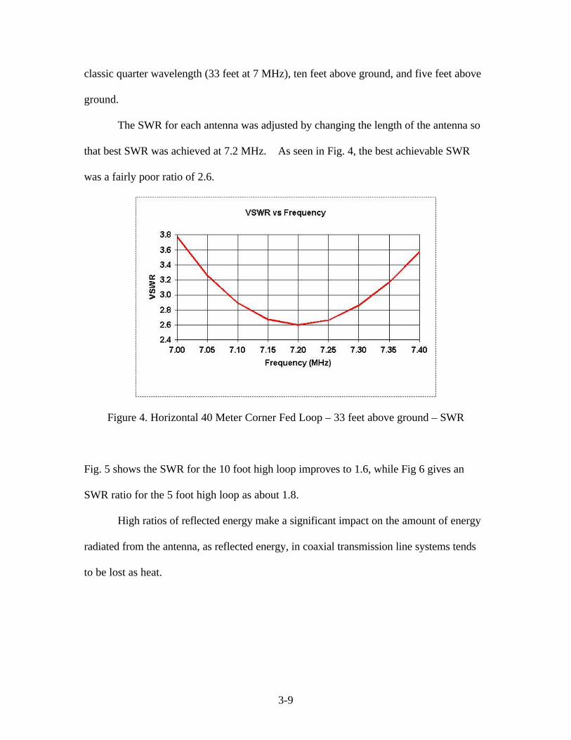
The SWR for each antenna was adjusted by changing the length of the antenna so

that best SWR was achieved at 7.2 MHz. As seen in Fig. 4, the best achievable SWR

was a fairly poor ratio of 2.6.

Figure 4. Horizontal 40 Meter Corner Fed Loop – 33 feet above ground – SWR

Fig. 5 shows the SWR for the 10 foot high loop improves to 1.6, while Fig 6 gives an

SWR ratio for the 5 foot high loop as about 1.8.

High ratios of reflected energy make a significant impact on the amount of energy

radiated from the antenna, as reflected energy, in coaxial transmission line systems tends

to be lost as heat.

3-10

Figure 5. Horizontal 40 Meter Corner Fed Loop – 10 feet above ground – SWR

Figure 6. Horizontal 40 Meter Corner Fed Loop – 5 feet above ground – SWR

Next, the antenna pattern for each of these antennas can be compared in azimuth

and elevation above the horizon.

3-11

Figure 7. Horizontal 40 Meter Corner Fed Loop – 33 feet above ground – Azimuth

Figure 8. Horizontal 40 Meter Corner Fed Loop – 10 feet above ground – Azimuth

3-12

Figure 9. Horizontal 40 Meter Corner Fed Loop – 5 feet above ground – Azimuth

There is a difference in these antenna patterns as the antenna is brought closer and

closer to the ground. Fig. 7 shows a close approximation to the ideal antenna pattern of a

full wavelength loop. Fig 8. shows the pattern diminishing as the antenna is brought

closer to the ground, while Fig 9. shows the pattern down more than 6 dB from isotropic

in azimuth. For our practical purpose, it is sufficient to note that the radiated power near

the horizon becomes lower and lower as the antenna is brought closer to the ground.

There is also significant difference in elevation above the horizon. It is these

comparisons that one finds the balance between ground absorption of the signal while

limiting the horizontal reception of the antenna.

Fig. 10 shows the zenith power of a quarter wavelength high loop as about 7 dB

above isotropic.

3-13

Figure 10. Horizontal 40 Meter Corner Fed Loop – 33 feet above ground – Elevation

Figure 11. Horizontal 40 Meter Corner Fed Loop – 10 feet above ground – Elevation

3-14

Figure 12. Horizontal 40 Meter Corner Fed Loop – 5 feet above ground – Elevation

Fig. 11 shows the 10 foot high loop is about 4 dB above isotropic, while the 5 foot

high version is at isotropic.

A similar analysis of horizontal dipoles follows. The simple dipole is supported

above average ground and is modeled as two equal length 1mm wires fed with a 50 ohm

unbalanced transmission line. The same modeling is accomplished for the three

antennas as in the previous example of the horizontal loop.

The antennas were adjusted for best SWR at 7.2 MHz. The SWR for the antennas

was slightly better than the best achievable SWR for the loop antennas.

Figs. 13 – 15 show the SWR for these horizontal dipoles is considerably more

favorable than the SWR for the loops. This favorable SWR means less signal power is

lost into the transmission line, and more is radiated.

3-15

Figure 13. 40 Meter Dipole – 33 Feet Above Ground – Standing Wave Ratio

Figure 14. 40 Meter Dipole – 10Feet Above Ground – Standing Wave Ratio

3-16

Figure 15. 40 Meter Dipole – 5 Feet Above Ground – Standing Wave Ratio

The azimuth patterns of Figs. 16 – 18, show the same relationship to height above

ground that was demonstrated for the horizontal loops. As the antenna is brought closer

to the ground, the pattern is distorted and diminished.

Figure 16. 40-Meter Dipole – 33 Feet Above Ground – Azimuth

3-17

Figure 17. 40 Meter Dipole – 10 Feet Above Ground – Azimuth

Figure 18. 40 Meter Dipole – 5 Feet Above Ground – Azimuth

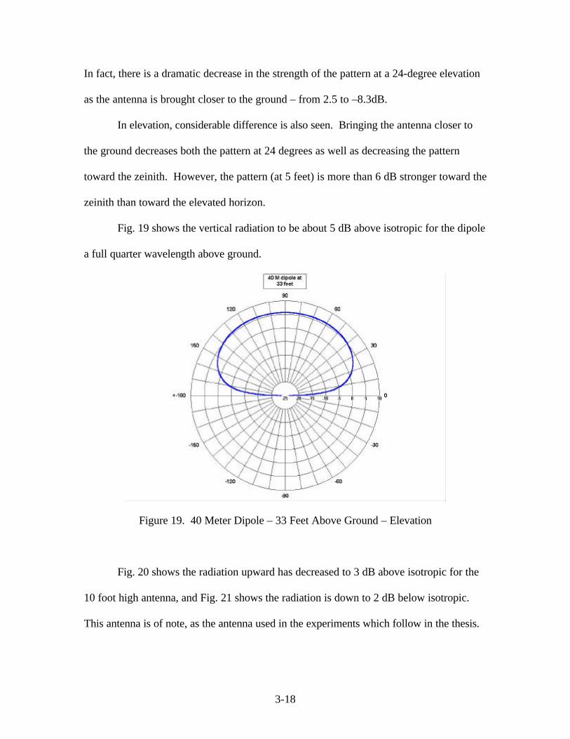
3-18

In fact, there is a dramatic decrease in the strength of the pattern at a 24-degree elevation

as the antenna is brought closer to the ground – from 2.5 to –8.3dB.

In elevation, considerable difference is also seen. Bringing the antenna closer to

the ground decreases both the pattern at 24 degrees as well as decreasing the pattern

toward the zeinith. However, the pattern (at 5 feet) is more than 6 dB stronger toward the

zeinith than toward the elevated horizon.

Fig. 19 shows the vertical radiation to be about 5 dB above isotropic for the dipole

a full quarter wavelength above ground.

Figure 19. 40 Meter Dipole – 33 Feet Above Ground – Elevation

Fig. 20 shows the radiation upward has decreased to 3 dB above isotropic for the

10 foot high antenna, and Fig. 21 shows the radiation is down to 2 dB below isotropic.

This antenna is of note, as the antenna used in the experiments which follow in the thesis.

3-19

Figure 20. 40 Meter Dipole – 10 Feet Above Ground – Elevation

Figure 21. 40 Meter Dipole – 5 Feet Above Ground – Elevation

3-20

Note that the strength of the upward directed pattern decreases significantly

between each of these steps toward the ground, but the selectivity of only receiving

signals from overhead increases at an even greater rate. The difference between

maximum vertical component comparing 10 feet with 5 foot heights goes from 3 dB to -

2 dB compared with isotropic, about a 5 dB delta. The maximum azimuth strength at 24

degrees above the horizon decreases from –4 dB to –8 dB, a difference of only 4 dB, but

resulting in very week reception of signals near the horizon.

The loop antenna’s pattern at 5 feet was about 2 dB stronger, but so was it’s

pattern toward the elevated horizon. Complicating this is the decreased SWR for the

dipole – 1.3 vs. 1.8 for the loop. A decision was made to use the dipole based on its

simple geometry. Either antenna would work reasonably well [23].

Next, consideration was given to the combination of antennas for two frequencies.

With emphasis on simplicity, design of an antenna was begun with a goal of including

two bands in one antenna with a single 50 ohm feed line to the transceiver.

Dual band antennas are not uncommon. In vertical, and Yagi beam antennas,

radio frequency traps are often placed in the antenna element so that at the higher of two

usable frequencies the LC trap acts as a tuned infinite resistance. At the lower frequency,

the trap is simply seen as an inductor, shortening the antenna [33].

Fan dipole antennas with separate elements are sometimes used for multi-band

HF antennas [30]. Starting with this idea, a crossed dipole antenna was designed for the

40-meter and the 80-meter bands. Such an antenna would allow choice of 40 or 80 meter

communication from the transceiver without any change to the antenna system. It is

likely that one of these two frequency bands would allow HF communication during

3-21

nearly every combination of the sun spot cycle, the cycle of seasons, and the diurnal

cycle.

The antenna was designed as two perpendicular dipole antennas, in the horizontal

plane, joined at the center insulator at which an unbalanced 50-ohm feed was attached.

The system was analyzed above a standard ground with the use of the Sommerfield

Integral option of NEC Win Plus.

Figure 22. 40-80 Meter Crossed Dipole – 33 Feet Above Ground –

Standing Wave Ratio

Fig. 22 shows the frequency response of the dual band antenna at 33 feet. Similar

SWR analysis for the ten and five foot high versions are included as Figs. 23 and 24. As

designed, the SWR is low at the center of the 40-meter and the 80-meter amateur bands.

3-22

Figure 23. 40-80 Meter Crossed Dipole – 10Feet Above Ground –

Standing Wave Ratio

Figure 24. 40-80 Meter Crossed Dipole – 5Feet Above Ground –

Standing Wave Ratio

Individual frequency sweeps for the 40 and 80 meter center points showed that

these antennas had individual SWR predictions of less than 2 SWR units.

3-23

The azimuth figures for the crossed dipole at the 3 heights follow:

Figure 25. 40-80 Meter Crossed Dipole – 33 Feet Above Ground – Azimuth

Figure 26. 40-80 Meter Crossed Dipole – 10 Feet Above Ground – Azimuth

3-24

Figure 27. 40-80 Meter Crossed Dipole – 5 Feet Above Ground – Azimuth

Figs. 25 –27 show the dual band azimuth patterns of the crossed dipole

configuration at all three design heights. Just as with the single band version, the amount

of grazing angle radiation decreases greatly for the lower antennas.

For the elevation figures, calculation and graphing was accomplished on each of

the major dimensions of the antenna. Because the antennas are crossed, each has a set of

two elevation plots.

In Figs. 28 – 33, the elevation pattern for each antenna is shown on each of the

primary axes, of the antenna pattern. As might be expected, the 40 meter patterns are

very similar to what was seen in the previous work. The 80 meter patterns are not as

efficient as the antenna gets closer to the ground.

3-25

Figure 28. 40-80 Meter Crossed Dipole – 33 Feet – Elevation at 0 degrees Azimuth

Figure 29. 40-80 Meter Crossed Dipole – 33 Feet – Elevation at 90 degrees Azimuth

3-26

Figure 30. 40-80 Meter Crossed Dipole – 10 Feet – Elevation at 0 degrees Azimuth

Figure 31. 40-80 Meter Crossed Dipole – 10 Feet – Elevation at 90 degrees Azimuth

3-27

Figure 32. 40-80 Meter Crossed Dipole – 5 Feet – Elevation at 0 degrees Azimuth

Figure 33. 40-80 Meter Crossed Dipole – 5 Feet – Elevation at 90 degrees Azimuth

Finally, the same comparison was made for two loop antennas. Several

configurations are possible. Using minimal landscape, one of the most efficient designs

3-28

is a corner fed pair of loops with the smaller loop sharing a part of two of the larger

loop’s sides.

Figure 34. 40-80 Meter Loops – 33 Feet Above Ground – Standing Wave Ratio

Figure 35. 40-80 Meter Loops – 10Feet Above Ground – Standing Wave Ratio

3-29

Figures of the antenna configurations can be examined in Appendix D.

Figure 36. 40-80 Meter Loops – 5Feet Above Ground – Standing Wave Ratio

The Standing Wave Ratio of this system is seen for the three heights in Figs. 34 –

38. Unfortunately, it is very difficult to trim the double loop antennas for precise SWR

on each band. For the 33-foot high antenna shown above, the detailed look at the

resonant frequencies is shown in Fig. 37. The SWRs of 4 and 8 for 40-meters and 80-

meters respectively, are for best achievable SWR and point out the large amount of

energy that would be lost in the transmission line if a 50 ohm line were used.

3-30

Figure 37. Double Loops – 33 Feet Above Ground – Standing Wave Ratio – 80 M

Figure 38. Double Loops – 33 Feet Above Ground – Standing Wave Ratio – 40 M

The Azimuth patterns are:

3-31

Figure 39. Double Loop – 33 Feet Above Ground – Azimuth

Figure 40. Double Loop – 10 Feet Above Ground – Azimuth

3-32

Figure 41. Double Loop – 5 Feet Above Ground – Azimuth

Figures 39 –41 depict the dual band azimuth patterns of the double loop antennas

at the 3 heights. The 40 meter portions of these patterns are distorted by the presence of

half wavelength antenna components in plane with the 40 meter quarter wavelength

components.

And finally the elevation patterns are shown in Figs. 42 –47. As with the crossed

dipoles, these antenna elevations are analyzed in each of the two major vertical planes of

radiation. For each antenna, because the load is applied to the corner, two elevations are

shown, one at 135 degrees of azimuth and the other at 225 degrees of azimuth. It may

not be surprising, with the half wavelength components at the shorter wavelength, that

the pattern has been distorted so that less energy is available for vertical transmission on

40 meters as there is available on 80 meters.

3-33

Figure 42. Double Loop – 33 Feet High – Elevation at 135 degrees Azimuth

Figure 43. Double Loop – 33 Feet High – Elevation at 225 degrees Azimuth

3-34

Figure 44. Double Loop – 10 Feet High – Elevation at 135 degrees Azimuth

Figure 45. Double Loop – 10 Feet High – Elevation at 225 degrees Azimuth

3-35

Figure 46. Double Loop – 5 Feet High – Elevation at 135 degrees Azimuth

Figure 47. Double Loop – 5 Feet High – Elevation at 225 degrees Azimuth

3-36

The pattern of the loop antennas is somewhat distorted in elevation and azimuth

for this system. While the main lobe of the antenna actually transmits more efficiently

than the crossed dipole near the earth, the inability to closely match SWR drives down

the performance of the antenna.

For completeness, a fourth antenna was briefly considered. Passive array

antennas are frequently used as directional antennas in azimuth. A classic antenna using

this principle is the Yagi antenna. With its reflector and directors, considerable gain can

be realized.

Unfortunately, all these designs require a reflector at something close to a quarter

wavelength behind a driven element to be efficient[6]. As has been seen in the forgoing,

this is going to be a very high antenna even for the 40-meter band. This exposes the

antenna to much more ground wave propagation which can have destructive interference.

Modeling for only the 10 foot height for the 40 Meter loop and dipole was

accomplished to examine whether these antennas would have any significant advantage

over their single element counterparts.

Figs. 48 –51 show the azimuth and elevation antenna patterns for a 10 foot high

antenna with a reflector (of 10 percent increased dimension) on the ground. Comparision

of these patterns with the corresponding patterns for the versions without reflector, show

no significant difference.

3-37

Figure 48. 40 Meter Loop at 10 feet with Reflector – Azimuth

Figure 49. 40 Meter Loop at 10 feet with Reflector – Elevation

3-38

Figure 50. 40 Meter Dipole at 10 feet with Reflector – Azimuth

Figure 51. 40 Meter Dipole at 10 feet with Reflector – Elevation

3-39

Description of Quantifiable Digital and Analog Communication Techniques

Part of the challenge of these experiments was the comparison of digital

communication techniques with analog voice techniques in a way that would be

meaningful to operational and emergency personnel.

A number of techniques can be used to compare digital communications systems.

The classic comparison would be the bit error rate [32].

The probability of bit error, BP for coherent BPSK is:

=

0

2

N

EQP b

B

where bE is the energy per bit, 0N is the noise energy, and where Q is given by

∫∞

−=

x

duu

xQ2

exp2

1)(

2

π

which is the complimentary error function.

The probability of symbol error, EP , for M-ary MFSK is bounded by:

)()1()(0N

EQMMP S

E −≤

where )(log 2 MEE BS = , the energy per symbol, M is then number of symbols, and K

is the smallest integer which fulfills: KM 2= .

In these communications, the output was a series of characters on a screen. The

characters were a product of several bits, and the bit errors rolled up into character errors

in a not always predictable manner.

Even with ASCII characters, each of which is coded by a fixed length bit

sequence, character errors do not necessarily relate directly to bit errors. Because of the

3-40

random nature of bit errors, it is possible to have more than one bit error in a character

error. It is also possible to have a bit error in a character and not have a character error –

not all bit errors result in character errors.

All of this is considerably complicated by the actual character representations

used by the COTS programs used in the experiment. Each program uses a similar (but

not identical) “varicode” to encode each character. The marker at the end of a character

is fixed as a multiple 0 bit with all the other characters not including the multiple 0 in

their bit string. This allows the determination of a bit string terminator and variable

length characters. Both systems assign common characters to the shortest bit

representations, while less common characters are given longer representations [19, 25].

For all these reasons, and for the simplicity of describing the results to emergency

radio operators, analysis is limited to character errors.

There were two digital methods used. The first was a simple binary phase shift

keying (BPSK) system designed to occupy minimum bandwidth for a communication

rate which would allow manual typing of messages between radio operators in a “chat

style” communication link. It was assumed that operators would not type any faster than

about 50 words per minute [25]. Words averaged 6 characters, and characters averaged 6

bits. The system transmits a bit rate of about 30 bits per second, given by

.

( )sec/

minsec/

// 3060

6650bits

chbitswordchwpm =

3-41

Applying standard digital techniques, since the system uses single side band

transmission, SSBW is the bandwidth of single side band required at radio frequency

SSSB RrW )1(2

1+=

where SR is the symbol rate in symbols per second, and r is the roll off rate of the

digital filter, here assumed to be 1. This means an additional 100 percent of bandwidth,

beyond that predicted by the Nyquist sampling theorem to account for roll off, and

HzWSSB 30=

which agrees very well with the advertised bandwidth of 31 Hz in PSK31.

The second digital technique uses 16-ary frequency shift keying (FSK) with

convolutional encoding, and interleaving used as forward error correction (FEC)

techniques. Together, these methods are effective in dealing with the fading, static

crashes, and interference that can occur on HF frequencies [19].

Knowing that the bit rate is doubled for FEC, the bit rate is given by

and the symbol rate is given by

.

The bandwidth can be calculated in the 16-ary case from the symbol rate. In an

uncorrelated MFSK signal, the bandwidth FSKBW is given by

( ) ( ) bbitsbitschbitswordchwpm R=== sec/sec/

minsec/

// 6023060

6650

sec/154

60S

bS K

RR ===

3-42

where

K is the smallest integer which fulfils KM 2≤ and

SR is the symbol rate in symbols per second.

Determination of expected error rates is complex for convolutional encoding

alone. The COTS system used here was designed with a data bit rate twice that required

for non-FEC communication. The bandwidth is nearly 10 times as wide as the BPSK

bandwidth, at about 250 Hz [19]. Both signals are narrow when compared with an

analog signal that utilizes a bandwidth of about 2000 Hz [34]. Trained operators can

often recognize the information in signals with center frequencies as close as 1000 Hz,

ignoring the low or high pitched audio from the neighboring single side band signals

[30].

In looking for a quantified test of the quality of an audio communication signal,

use was made of the clinical tests used by aerospace medicine specialists in diagnosis of

operationally relevant hearing loss in trained aviators. Within the Air Force medical

instructions, are several tests that allow a flight surgeon to send a word with a standard

voice and have the pilot on the other end of a communication link circle one of three

similar words [31].

The results of this test vary from one test physician to another, but each examiner

becomes familiar with the results they expect from pilots. These results are remarkably

( ) HzRMBW SFSK 255)15(171 ==+≈

3-43

similar between normal hearing pilots and only differ in a significant way when the pilot

is having trouble with his hearing.

Different physicians have slightly different results from the tests, as it is possible

for the test giver to attempt to make the words very clear or to say them more as words in

normal conversation. This is a known bias to the test, and is impossible to control to an

exact extent unless recordings are used instead of human examiners [31].

Unfortunately, recordings do not make the sorts of very automatic corrections to

prevailing radio conditions that trained operators make. This kind of correction leads to

some analytic confusion, but much more accurately represents what human operators

actually do in the field.

Both operators in these experiments agreed to not consciously over-pronounce

words or repeat them unless it was clear that a word had not been sent. Never was a word

repeated because it had not been understood the first time. For the few cases that the

word was not clearly understood, the receiving operator made a best guess.

The words are chosen to sound alike, not to look alike. It comes as no surprise

that the operators were able to choose the word correctly more often with the digital

modes than with the analog single side band mode. It may also come as no surprise to

the field operator that a more accurate message can be received by digital methods than

by audio.

But using the digital modes with these word lists and by comparison with the

actual transcript from the two sites digital communications was designed to not only find

the number of character errors, but to compare the words answered correctly with the

words that should have been able to be answered correctly from the transcript.

3-44

By knowing the number of words answered correctly, as compared with the

number that should have been able to be answered correctly, some estimate of the

number of word errors an operator makes due to human factors. Using this information,

inference can be made about the true analog error rate as compared with the recorded

analog error rate.

The word lists used in the experiment can be viewed in Appendix B.

Data Collection

The data was collected from December 2001 to January 2002. The solar cycle

was beginning to wane, though conditions for HF propagation were still good. The

previous peak had occurred about one year previous to these tests. The data were all

collected with a set combination of antennas. The WS8B site was a sloping inverted V

antenna. The WS8G antenna was a horizontal dipole at 5 feet above the natural ground.

All experiments were conducted on the 40 M amateur band. The analog portions

of the tests were conducted at or near 7.16 MHz, and the digital portions were conducted

at 7.065 MHz. These frequencies were chosen to comply with the established band plan

for the amateur service.

The method selected for collection of data was for each operator to send three

different 50-word tests. Each operator sent and received each of three modes. From each

geographic site the mobile operator took, there is a set of 6 tests. Each test has

approximately 215 characters.

Words were sent in blocks of 5 regardless of mode. The sending operator would

wait for an acknowledgement from the receiving operator before continuing. Groups of

words were not sent a second time, even when the operator knew they had difficulty with

3-45

one of the words for any reason. Occasionally, when it was agreed by both operators that

a word that should have been sent had not been sent at all, the word was sent on special

request. This happened very occasionally in the analog mode with the first or last word

of a group of 5.

During each test, the receiving operator filled in a multiple answer sheet. Three

choices were available for each transmitted word, and the operator circled their best guess

of the correct word. The sheets were labeled to show the date, operator, mode,

frequency, and distance between stations. The sheets were collected and were the

primary data source for parts of the analysis.

In addition, a character-by-character computer log was maintained on each

operator’s computer system during the digital portions of the testing. These logs were

stored and later printed. They became the basis for character-by-character analysis of the

digital data.

Several other data collection techniques, as follows, were considered and rejected.

While other researchers may find these data techniques useful, their collection at this

stage was not conclusively necessary.

An additional analog data source that was collected were audio recordings of the

single side band data sessions. This information would have been valuable in the

analyzing human error, by allowing a second trained operator to listen to the recorded

source and attempt to select correct words.

Another analog data source could have been a video recording or digital storage

of the sound card’s spectral power waterfall display. From this display, the operator can

observe the interplay of nearby signals and broadband noise sources. Together with an

3-46

audio recording of the digital signal, a further impression can be gleaned for analysis.

Unfortunately, no simple and expedient method to analyze or present this as anything

more than anecdotal data was discovered.

Mobile Site Description

Data was collected from four separate geographic areas. These were chosen to

represent several of the difficult field situations that exist in the relative close range. The

usefulness of HF communications at great distance has been previously described in

reasonable depth – as has the problem of skip propagation. The characteristics of VHF

and UHF using LOS communication are also well described. These locations were

chosen to represent places where UHF and VHF would be blocked and from which short-

range HF contacts might be difficult.

The experiment was conducted with a fixed station and a mobile station. The

fixed station, WS8B, whose antenna system was previously described, is attached to a

suburban home. At an elevation of about 700 feet above sea level, it sits on what was

once rolling farmland. The terrain is reasonably flat, and the station is in neither a valley

nor on a high point with regard to the surrounding area. For a topographic map of the site

with orientation of the antenna, see Fig. 52. Measured Global Positioning Satellite GPS

coordinates match the coordinates on the topographic map and are available upon request

from the author. All mobile sites were to the west of WS8B’s location.

For all maps that follow, North is toward the top of the page, and the scale is

1:25000.

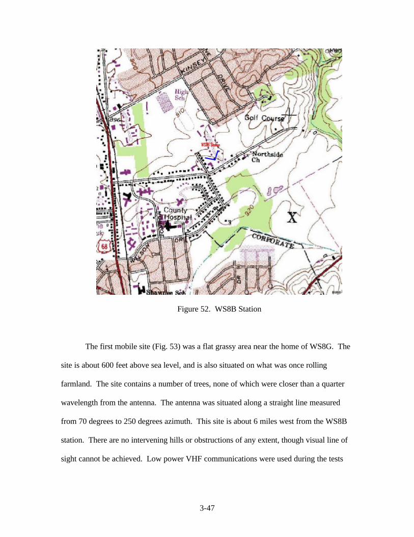
3-47

Figure 52. WS8B Station

The first mobile site (Fig. 53) was a flat grassy area near the home of WS8G. The

site is about 600 feet above sea level, and is also situated on what was once rolling

farmland. The site contains a number of trees, none of which were closer than a quarter

wavelength from the antenna. The antenna was situated along a straight line measured

from 70 degrees to 250 degrees azimuth. This site is about 6 miles west from the WS8B

station. There are no intervening hills or obstructions of any extent, though visual line of

sight cannot be achieved. Low power VHF communications were used during the tests

3-48

from this location to coordinate final configuration of the radio and computer systems,

confirming the presence of line of sight to 147 MHz communication.

Figure 53. WS8G Home Station

The second mobile site, 23 miles west-northwest from the WS8B station, was

chosen to present a very difficult terrain for line of sight and ground wave transmission.

This spot (Fig. 54), in the Englewood Reserve, was situated in a 150-foot (verified by

GPS measurement) deep valley with a very steep rocky and forested wall immediately

east of the mobile position. The position of this wall was directly between the mobile

station and the fixed WS8B station. Simplex communication between the stations on

VHF could not be achieved. Repeater based communication using a high tower near the

3-49

WS8B position was also not possible. Even cell telephone communication was very

difficult, though the station was within a few miles of Englewood, Ohio and Interstate 70.

The antenna was sited nearly east and west, over a frozen grassy picnic area. Trees were

present, but none were within a quarter wavelength of the antenna.

Figure 54. Englewood Reserve Station

The third mobile site, 46 miles west-south-west of the fixed WS8B station, was

situated in a rolling valley; about a hundred feet lower than the surrounding countryside,

near the lake in Hueston Woods State Park. This site is illustrated in Fig. 55. The

antenna was sited along a 10-foot wide east-west strip of grass in a parking lot at the state

park lodge.

3-50

Figure 55. Hueston Woods Station

The last mobile site (Figs. 56 - 57) was chosen to explore the sorts of difficulties

urban canyons impose on line of sight communication. Though only 11 miles from the

WS8B site, this spot, on a narrow grassy strip next to a large metal clad building,

represents city streets surrounded by tall buildings - the urban canyon. This site is on the

lower part of Wright Patterson AFB, about a hundred feet below the surrounding

countryside, with a hillside between it and the WS8B station. The road and the hillside

are perpendicular to a line connecting the stations.

3-51

Figure 56. Wright-Patterson Station - Topographic

Radio conditions for most of the tests were about average on the HF bands with

the exception of the testing from this urban canyon. A contest on the digital bands was in

full swing when this testing was accomplished. There were a multitude of competing

stations on the digital sub-bands.

3-52

Figure 57. Wright-Patterson Station - Satellite Photo

Analysis Procedures

The data from the experiments was analyzed in two ways. Obviously, the answer

sheets were graded, so that conclusions could be drawn from the errors. The digital data

logs were also examined toward several ends.

For the answer sheets, the known list of sent words was used to correct the words

the receiver believed they had heard. This analysis was not conducted in the field, and

the operator had no feedback as to their success during the experiment. There was

3-53

therefore no concurrent knowledge of how the radio operator was doing in comparison

with their other tests or in comparison with the other operator.

Both operators had access to the correct words, but the lists were found to be far

too long to attempt to memorize the word order. The operators had discussed data

collection previous to the tests and had decided that the best way to answer the questions

was to make a first choice and then stick with it. There was no evidence on the answer

sheets of corrections to answers once chosen.

The digital data consists of eight ASCII streams, one from each operator for each

time the mobile WS8G station moved. These streams include all the characters sent by

the operator, and the decoded characters obtained from the program’s analysis of the

received waveform.

Within each stream, there are four lists of 50 words. Two lists are the characters

sent by the operator and are assumed for these purposes to be an accurate account of the

keyboard entries made by the operator. The other two lists are assumed to be the

characters as they appeared to the receiving operator on their computer screen. The only

discrepancy from this is the use of the back space key. The ASCII stream accurately

shows all backspace entries made by the operators. The operator often did not see these

backspaces or have time to process the information removed by the backspacing before it

was replaced with new information.

The operators made a number of typing errors. In almost no case, did the typing

error lead to a missed word on the answer sheet. All typing errors were compared from

one computer’s log to the other computer’s log to determine the character error rate,

regardless of whether an operator answered correctly on the answer sheet.

3-54

Of interest, in nearly every instance when a single character error was sent – a

misspelled word – the receiving operator chose the correct word on the answer sheet.

The same cannot be said for correctly spelled words. Of the words incorrectly answered

on the sheet, a number of these errors were attributable to the operator reading the right

word on the computer screen and then circling the wrong word on the answer sheet. To

err is human.

Mathematically this can be expressed as follows:

eceword HHChE +−= )(

where wordE is the total number of word errors, eCh is the number of words coming

through the channel with an error, cH is the number of words corrected by the operator,

and eH is the number of words recorded in error by the operator.

4-1

IV. Results

This work is a descriptive study with conclusions drawn from qualitative analysis

of data collected. At one level, it describes the quantity of information that can be passed

with NVIS communication techniques. From a human factors perspective, it examines

the interaction of trained radio operators with technology.

Performance Testing

As seen in Fig. 58, the overall test performance for analog accuracy by both

operators was 92 percent. Operator A’s scores were consistently better than scores for

operator B.

Analog Voice

0

10

20

30

40

50

60

70

80

90

100

WS8G Station Englewood Hueston Woods Urban Canyon

per

cen

t co

rrec

t

Operator A

Operator B

Figure 58. Voice Scores for Each Location - Operator A and B.

This could have been improved if the operators had used a standard phonetic

alphabet to spell out each word as though it were a critical item of information. For

4-2

example, phase would become “Poppa Hotel Alpha Sierra Echo.” This method was not

separately examined for this work.

The overall test performance for Binary Phase Shift Keying (BPSK) was 98

percent. Fig. 59 shows BPSK performance was better than analog voice.

BPSK

0

10

20

30

40

50

60

70

80

90

100

WS8G Station Englewood Hueston Woods Urban Canyon

per

cen

t co

rrec

t

Operator A

Corrected

Operator B

Corrected

Figure 59. Percent of Words Correct for Each Location BPSK

The test performance for MFSK with convolutional encoding and interleaving

seen in Fig. 60 was better than analog voice. Fig. 61 shows there was no consistent

difference between the two digital modes except on one day when there was a higher

level of interfering signals than on any of the other days.

4-3

MFSK16

0

10

20

30

40

50

60

70

80

90

100

WS8G Station Englewood HuestonWoods

Urban Canyon

per

cen

t co

rrec

t

Operator A

Corrected

Operator B

Corrected

Figure 60. Percent of Words Correct for Each Location MFSK.

Character Errors

85

86

87

88

89

90

91

92

93

94

95

96

97

98

99

100

WS8G Station Englewood HuestonWoods

Urban Canyon

per

cen

t co

rrec

t

BPSK

MFSK16

Figure 61. Percent Character Errors – BPSK and MFSK

4-4

The actual performance of the digital modes was better than the human recording

of the digital modes. Both Figs. 59 and 60 show that if the operators had not made errors,

the accuracy rate would have been better than the test performance indicates.

Based on this collected data, Fig. 62 demonstrates the clear differences between

the error rates for the three modes. Examining the overall performance of the operators

(without correction) for the three modes, it is clear that the digital modes did better than

the analog voice.

Comparison of Modes

80

82

84

86

88

90

92

94

96

98

100

WS8G Station Englewood Hueston Woods Urban Canyon

per

cen

t co

rrec

t (u

nco

rrec

ted

)

Voice

BPSK

MFSK16

Figure 62. Percent Character Errors – Mode Comparison Overall

An assumption can be made that the human errors in analog voice test

performance also degraded performance in comparison with perfect performance. It may

be true that up to about 2 percent of errors are “careless” errors. There is insufficient

data to suppose either perfect performance by the operators on voice or to suppose that

the error rate on voice is the same as that on digital performance.

4-5

Several factors contribute to the improved performance of digital communication

vs. analog communication. A significant contribution to this error rate is the designed

difficulty of distinguishing the spoken words in the test sets. The words were developed

to sound alike, not necessarily to look alike in text. This same human factor is also

reflected in real world communications, when human voice is used for analog

communication.

An additional factor is the time dispersion of the digital signal as opposed to the

analog spoken word. Transient atmospheric disturbances have an effect on digital

characters, but the same disturbance can entirely render a spoken word meaningless.

Further, an operator’s temporary lapse of attention during the analog testing

resulted in an unrecoverable error. On the digital testing, the transmitted symbols

remained on the screen until scrolling off. Lapsed attention during a digital test could be

corrected by looking back at the screen a second time.

5-1

V. Conclusions and Recommendations for Further Research

It is practical to construct a medium range emergency communication system

using low power transceivers and a lightweight portable Near Vertical Incidence

Skywave (NVIS) antenna system on HF radio bands. Communications can be conducted

in analog single side band audio, or may utilize one of several COTS digital systems that

rely on a laptop computer and the digital signal processing capability of a computer

sound card. For this research, radio stations were set up in locations representing the

local conditions that could exist for emergency response parties.

Conclusions The first station pair represents a near line-of-sight (LOS) condition. For this

portable setup alone, VHF LOS communication was possible across this distance with

similar power output as what was used in the HF experiment. The portable station’s

antenna was designed in such a way that the ground wave and LOS wave would be

reduced in intensity, allowing the bulk of the received energy to be received from the sky

wave. The distance and reflective components of the sky wave make it a riskier

propagation path, but the communication was still able to succeed.

The second station pair was chosen at a reasonably close distance, but with lots of

rock and dirt between the stations. In a 150-foot deep hole at this distance, there would

not have been any significant ground wave in the valley. This station represents many of

the situations that may occur in rural hilly environments and mountain valleys.

The third station pair was chosen to represent the problems of a radio

environment near the radio horizon, and down a hill. It is this sort of environment that

suffers from an inability to maintain VHF links even with very tall towers at the base

5-2

station. It is this same sort of place that suffers from the strong signal degradation from

being in a skip area.

The fourth station pair was added to simulate the difficult radio environment of an

urban canyon. In such an area, VHF and UHF traffic is of little use unless very tall

buildings have working repeaters. Even when such repeaters exist, they may be jammed

with too much traffic during an emergency. This fourth station pair was added to test the

idea of using sky waves to communicate from the surface streets surrounded by the

concrete and metal of a modern city. Such communication can be conducted even when

the tops of the buildings are inaccessible and power systems have been turned off.

The result of all station pairs was a resounding success for all communication

modes. The received signal strength was usable in all modes. Error rates were

comparable to other forms of radio communication. Voice analog signals had an word

recognition error rate of between eight and twelve percent. Digital mode error rates were

all less than 5 percent.

Conclusions can be drawn about the human element in these experiments. As a

physician, these elements are amongst the most fascinating of the results. Almost a two

percent error rate can be attributed to the two operators in their choice of right answers

for the digital portions of the testing. Nothing can be inferred about the error rate

involving audio communication from this, other than a strong probability that the error

rate was not zero.

While an examination of the causes of human error is outside the scope of this

thesis, the existence of such error must be recognized as affecting the results of the

5-3

experiment. This is as it should be, because human operators of the system are expected

in any emergency communication system.

Recommendations for Further Research The strength of the signals begs work at lower power levels. One watt or even a

half-watt are reasonable goals for further experiments. Such power levels would improve

efficiency of communications systems that need to be carried in a backpack. This would

be the direction one could go if there was need for a very lightweight radio system to be

carried while running long distances, or climbing rock escarpments.

Other goals for further research would be to apply these antennas to spread

spectrum communication. While the bandwidth of the HF frequencies is not very large

compared with the available bandwidth at higher frequencies, enough is available to pass

small data streams across perhaps a tenth of a megahertz up to a full megahertz. With a

very small power level, such communications may not be easily discovered. It is likely

that such a data stream spread only over the available audio bandwidth of an amateur

radio transceiver and a commercial computer sound card could be identified, but when

spread out 50 times more thinly, it will be more difficult.

A-1

Appendix A – NEC Input Cards From these wire lengths, and orientation, the model results can be replicated. A copy of the computer files with these values will be held by Dr Terzuoli, the Thesis Advisor.

40 M Vertical CM CE GW 1 20 0 0 0.1 0 0 32.75 0.0010565 GW 2 10 0 0 0.1 32.75 0 0.1 0.0010565 GW 3 10 0 0 0.1 -32.75 0 0.1 0.0010565 GW 4 10 0 0 0.1 0 32.75 0.1 0.0010565 GW 5 10 0 0 0.1 0 -32.75 0.1 0.0010565 GW 30901 1 9901.0000 9901.0000 9901.0000 9901.0001 9901.0001 9901.0001 .00001 GS 0 0 .30479 GE 1 GN 2 0 0 0 13.0 0.005 EX 0 30901 1 0 1 0 LD 5 1 1 20 5.8001E7 LD 5 2 1 10 5.8001E7 LD 5 3 1 10 5.8001E7 LD 5 4 1 10 5.8001E7 LD 5 5 1 10 5.8001E7 NT 30901 1 1 1 0 0 0 1 0 0 FR 0 9 0 0 7 0.05 RP 0 1 360 1000 66 1 1 1 FR 0 9 0 0 7 0.05 RP 0 181 1 1000 -90 0 1 1 EN

40 M Loop at 33 feet CM CE GW 1 3 0.2 0 33 0 0.2 33 0.0013321 GW 2 10 0.2 0 33 35.2 0 33 0.0013321 GW 3 10 35.2 0 33 35.2 35.2 33 0.0013321 GW 4 10 35.2 35.2 33 0 35.2 33 0.0013321 GW 5 10 0 35.2 33 0 0.2 33 0.0013321 GS 0 0 .30479 GE 1 GN 2 0 0 0 13.0 0.005 EX 0 1 2 0 1 0 LD 5 1 1 3 5.8001E7 LD 5 2 1 10 5.8001E7 LD 5 3 1 10 5.8001E7

A-2

LD 5 4 1 10 5.8001E7 LD 5 5 1 10 5.8001E7 FR 0 9 0 0 7 0.05 RP 0 1 360 1000 66 1 1 1 FR 0 9 0 0 7 0.05 RP 0 181 1 1000 -90 0 1 1 EN

40 M Loop at 10 feet CM CE GW 1 3 0.2 0 10 0 0.2 10 0.0013321 GW 2 10 0.2 0 10 34.75 0 10 0.0013321 GW 3 10 34.75 0 10 34.75 34.75 10 0.0013321 GW 4 10 34.75 34.75 10 0 34.75 10 0.0013321 GW 5 10 0 34.75 10 0 0.2 10 0.0013321 GS 0 0 .30479 GE 1 GN 2 0 0 0 13.0 0.005 EX 0 1 2 0 1 0 LD 5 1 1 3 5.8001E7 LD 5 2 1 10 5.8001E7 LD 5 3 1 10 5.8001E7 LD 5 4 1 10 5.8001E7 LD 5 5 1 10 5.8001E7 FR 0 9 0 0 7 0.05 RP 0 1 360 1000 66 1 1 1 FR 0 9 0 0 7 0.05 RP 0 181 1 1000 -90 225 1 1 EN

40 M Loop at 5 feet CM CE GW 1 3 0.2 0 5 0 0.2 5 0.0013321 GW 2 10 0.2 0 5 34.25 0 5 0.0013321 GW 3 10 34.25 0 5 34.25 34.25 5 0.0013321 GW 4 10 34.25 34.25 5 0 34.25 5 0.0013321 GW 5 10 0 34.25 5 0 0.2 5 0.0013321 GS 0 0 .30479 GE 1 GN 2 0 0 0 13.0 0.005 EX 0 1 2 0 1 0 LD 5 1 1 3 5.8001E7 LD 5 2 1 10 5.8001E7 LD 5 3 1 10 5.8001E7

A-3

LD 5 4 1 10 5.8001E7 LD 5 5 1 10 5.8001E7 FR 0 9 0 0 7 0.05 RP 0 1 360 1000 66 1 1 1 FR 0 9 0 0 7 0.05 RP 0 181 1 1000 -90 135 1 1 EN

40 M Dipole at 33 feet CM CE GW 1 21 0 32.9 33 0 -32.9 33 0.0013321 GS 0 0 .30479 GE 1 GN 2 0 0 0 13.0 0.005 EX 0 1 11 0 1 0 LD 5 1 1 21 5.8001E7 FR 0 9 0 0 7 0.05 RP 0 1 360 1000 66 1 1 1 FR 0 9 0 0 7 0.05 RP 0 181 1 1000 -90 0 1 1 EN

40 M Dipole at 10 feet CM CE GW 1 21 0 33 10 0 -33 10 0.0013321 GS 0 0 .30479 GE 1 GN 2 0 0 0 13.0 0.005 EX 0 1 11 0 1 0 LD 5 1 1 21 5.8001E7 FR 0 9 0 0 7 0.05 RP 0 1 360 1000 66 1 1 1 FR 0 9 0 0 7 0.05 RP 0 181 1 1000 -90 0 1 1 EN

40 M Dipole at 5 feet CM CE GW 1 21 0 33 5 0 -33 5 0.0013321 GS 0 0 .30479 GE 1 GN 2 0 0 0 13.0 0.005 EX 0 1 11 0 1 0

A-4

LD 5 1 1 21 5.8001E7 FR 0 9 0 0 7 0.05 RP 0 1 360 1000 66 1 1 1 FR 0 9 0 0 7 0.05 RP 0 181 1 1000 -90 0 1 1 EN

40 M and 80 M Double Loop at 33 feet CM CE GW 1 3 0.5 0 33 0 0.5 33 0.0013321 GW 2 10 0.5 0 33 34.5 0 33 0.0013321 GW 3 10 34.5 0 33 73 0 33 0.0013321 GW 4 20 73 0 33 73 73 33 0.0013321 GW 5 20 73 73 33 0 73 33 0.0013321 GW 6 10 0 73 33 0 34.5 33 0.0013321 GW 7 10 0 34.5 33 0 0.5 33 0.0013321 GW 8 10 34.5 0 33 34.5 34.5 33 0.0013321 GW 9 10 34.5 34.5 33 0 34.5 33 0.0013321 GS 0 0 .30479 GE 1 GN 2 0 0 0 13.0 0.005 EX 0 1 2 0 1 0 LD 5 1 1 3 5.8001E7 LD 5 2 1 10 5.8001E7 LD 5 3 1 10 5.8001E7 LD 5 4 1 20 5.8001E7 LD 5 5 1 20 5.8001E7 LD 5 6 1 10 5.8001E7 LD 5 7 1 10 5.8001E7 LD 5 8 1 10 5.8001E7 LD 5 9 1 10 5.8001E7 FR 0 8 0 0 3.7 0.5 RP 0 1 360 1000 66 1 1 1 FR 0 8 0 0 3.7 0.5 RP 0 181 1 1000 -90 0 1 1 EN

40 M and 80 M Double Loop at 10 feet CM CE GW 1 3 0.5 0 10 0 0.5 10 0.0013321 GW 2 10 0.5 0 10 34.5 0 10 0.0013321 GW 3 10 34.5 0 10 73 0 10 0.0013321 GW 4 20 73 0 10 73 73 10 0.0013321

A-5

GW 5 20 73 73 10 0 73 10 0.0013321 GW 6 10 0 73 10 0 34.5 10 0.0013321 GW 7 10 0 34.5 10 0 0.5 10 0.0013321 GW 8 10 34.5 0 10 34.5 34.5 10 0.0013321 GW 9 10 34.5 34.5 10 0 34.5 10 0.0013321 GS 0 0 .30479 GE 1 GN 2 0 0 0 13.0 0.005 EX 0 1 2 0 1 0 LD 5 1 1 3 5.8001E7 LD 5 2 1 10 5.8001E7 LD 5 3 1 10 5.8001E7 LD 5 4 1 20 5.8001E7 LD 5 5 1 20 5.8001E7 LD 5 6 1 10 5.8001E7 LD 5 7 1 10 5.8001E7 LD 5 8 1 10 5.8001E7 LD 5 9 1 10 5.8001E7 FR 0 8 0 0 3.7 0.5 RP 0 1 360 1000 66 1 1 1 FR 0 8 0 0 3.7 0.5 RP 0 181 1 1000 -90 225 1 1 EN

40 M and 80 M Double Loop at 5 feet CM CE GW 1 3 0.5 0 5 0 0.5 5 0.0013321 GW 2 10 0.5 0 5 33 0 5 0.0013321 GW 3 10 33 0 5 73 0 5 0.0013321 GW 4 20 73 0 5 73 73 5 0.0013321 GW 5 20 73 73 5 0 73 5 0.0013321 GW 6 10 0 73 5 0 33 5 0.0013321 GW 7 10 0 33 5 0 0.5 5 0.0013321 GW 8 10 33 0 5 33 33 5 0.0013321 GW 9 10 33 33 5 0 33 5 0.0013321 GS 0 0 .30479 GE 1 GN 2 0 0 0 13.0 0.005 EX 0 1 2 0 1 0 LD 5 1 1 3 5.8001E7 LD 5 2 1 10 5.8001E7 LD 5 3 1 10 5.8001E7 LD 5 4 1 20 5.8001E7 LD 5 5 1 20 5.8001E7 LD 5 6 1 10 5.8001E7

A-6

LD 5 7 1 10 5.8001E7 LD 5 8 1 10 5.8001E7 LD 5 9 1 10 5.8001E7 FR 0 8 0 0 3.7 0.5 RP 0 1 360 1000 66 1 1 1 FR 0 8 0 0 3.7 0.5 RP 0 181 1 1000 -90 135 1 1 EN

40 M and 80 M Crossed Dipole at 33 feet CM CE GW 1 3 -0.5 -0.5 33 0.5 0.5 33 0.0013321 GW 2 10 -32.75 0 33 -0.5 -0.5 33 0.0013321 GW 3 10 32.75 0 33 0.5 0.5 33 0.0013321 GW 4 20 0 -64 33 -0.5 -0.5 33 0.0013321 GW 5 20 0 64 33 0.5 0.5 33 0.0013321 GS 0 0 .30479 GE 1 GN 2 0 0 0 13.0 0.005 EX 0 1 2 0 1 0 LD 5 1 1 3 5.8001E7 LD 5 2 1 10 5.8001E7 LD 5 3 1 10 5.8001E7 LD 5 4 1 20 5.8001E7 LD 5 5 1 20 5.8001E7 FR 0 9 0 0 7 0.05 RP 0 1 360 1000 66 1 1 1 FR 0 9 0 0 7 0.05 RP 0 181 1 1000 -90 0 1 1 EN

40 M and 80 M Crossed Dipole at 10 feet CM CE GW 1 3 -0.5 -0.5 10 0.5 0.5 10 0.0013321 GW 2 10 -33 0 10 -0.5 -0.5 10 0.0013321 GW 3 10 33 0 10 0.5 0.5 10 0.0013321 GW 4 20 0 -64 10 -0.5 -0.5 10 0.0013321 GW 5 20 0 64 10 0.5 0.5 10 0.0013321 GS 0 0 .30479 GE 1 GN 2 0 0 0 13.0 0.005 EX 0 1 2 0 1 0 LD 5 1 1 3 5.8001E7 LD 5 2 1 10 5.8001E7

A-7

LD 5 3 1 10 5.8001E7 LD 5 4 1 20 5.8001E7 LD 5 5 1 20 5.8001E7 FR 0 8 0 0 3.7 0.5 RP 0 1 360 1000 66 1 1 1 FR 0 8 0 0 3.7 0.5 RP 0 181 1 1000 -90 270 1 1 EN

40 M and 80 M Crossed Dipole at 5 feet CM CE GW 1 3 -0.5 -0.5 5 0.5 0.5 5 0.0013321 GW 2 10 -32.75 0 5 -0.5 -0.5 5 0.0013321 GW 3 10 32.75 0 5 0.5 0.5 5 0.0013321 GW 4 20 0 -63.5 5 -0.5 -0.5 5 0.0013321 GW 5 20 0 63.5 5 0.5 0.5 5 0.0013321 GS 0 0 .30479 GE 1 GN 2 0 0 0 13.0 0.005 EX 0 1 2 0 1 0 LD 5 1 1 3 5.8001E7 LD 5 2 1 10 5.8001E7 LD 5 3 1 10 5.8001E7 LD 5 4 1 20 5.8001E7 LD 5 5 1 20 5.8001E7 FR 0 8 0 0 3.7 0.5 RP 0 1 360 1000 66 1 1 1 FR 0 8 0 0 3.7 0.5 RP 0 181 1 1000 -90 270 1 1 EN

40 M Loop with reflector at 10 feet CM CE GW 1 3 0.2 0 10 0 0.2 10 0.0013321 GW 2 10 0.2 0 10 34.75 0 10 0.0013321 GW 3 10 34.75 0 10 34.75 34.75 10 0.0013321 GW 4 10 34.75 34.75 10 0 34.75 10 0.0013321 GW 5 10 0 34.75 10 0 0.2 10 0.0013321 GW 6 10 -1 -1 0.02 35.75 -1 0.02 0.0013321 GW 7 10 35.75 -1 0.02 35.75 35.75 0.02 0.0013321 GW 8 10 35.75 35.75 0.02 -1 35.75 0.02 0.0013321 GW 9 10 -1 35.75 0.02 -1 -1 0.02 0.0013321 GS 0 0 .30479 GE 1

A-8

GN 2 0 0 0 13.0 0.005 EX 0 1 2 0 1 0 LD 5 1 1 3 5.8001E7 LD 5 2 1 10 5.8001E7 LD 5 3 1 10 5.8001E7 LD 5 4 1 10 5.8001E7 LD 5 5 1 10 5.8001E7 LD 5 6 1 10 5.8001E7 LD 5 7 1 10 5.8001E7 LD 5 8 1 10 5.8001E7 LD 5 9 1 10 5.8001E7 FR 0 9 0 0 7 0.05 RP 0 1 360 1000 66 1 1 1 FR 0 9 0 0 7 0.05 RP 0 181 1 1000 -90 225 1 1 EN

40 M Dipole with reflector at 10 feet CM CE GW 1 21 0 33 10 0 -33 10 0.0013321 GW 2 20 0 34 0.02 0 -34 0.02 0.0013321 GS 0 0 .30479 GE 1 GN 2 0 0 0 13.0 0.005 EX 0 1 11 0 1 0 LD 5 1 1 21 5.8001E7 LD 5 2 1 20 5.8001E7 FR 0 9 0 0 7 0.05 RP 0 1 360 1000 66 1 1 1 FR 0 9 0 0 7 0.05 RP 0 181 1 1000 -90 0 1 1 EN

B-1

Appendix B – Word Lists . LIST 1 LIST 2 LIST 3 1. LATE 1. LAID 1. LANE 2. LEAN 2. LEAD 2. LEAK 3. HAD 3. HATCH 3. HASH 4. SPEED 4. SPEECH 4. SPEAK 5. GROSS 5. GROPE 5. GROVE 6. BUST 6. BUDGE 6. BUMP 7. REEL 7. READ 7. REACH 8. SLAP 8. SLAM 8. SLAB 9. HALF 9. HAVE 9. HANG

10. CHASE 10. CHANGE 10. CHAIN 11. GRADE 11. GRAZE 11. GREAT 12. TRIP 12. TRICK 12. TRIM 13. CREEP 13. CREAM 13. CREEK 14. FADE 14. PHASE 14. FACE 15. SUN 15. SUNK 15. SUB 16. PLACE 16. PLANE 16. PLATE 17. CAME 17. CASE 17. CAGE 18. CHICKS 18. CHIPS 18. CHILLS 19. SLANT 19. SLASH 19. SLACK

20. LEG 20. LED 20. LESS 21. MAZE 21. MAIN 21. MAKE 22. RAISE 22. RAID 22. RATE 23. HUT 23. HUNG 23. HUNT 24. JUDGE 24. JUNK 24. JUMP 25. LATCH 25. LAND 25. LAP 26. NET 26. NEST 26. NEXT 27. FLANK 27. FLAP 27. FLAT 28. SEAT 28. SEEM 28. CEASE 29. KEEN 29. KEEP 29. KEYS

30. WISH 30. WIND 30. WING 31. CLASP 31. CLAMP 31. CLAP 32. SUMP 32. SUCH 32. SOME 33. PATH 33. PAD 33. PAST 34. BLADE 34. BLAZE 34. BLAME 35. FAN 35. FAT 35. FAST 36. LOOSE 36. LOOP 36. LUBE 37. CHAFF 37. CHAP 37. CHAT 38. FEET 38. FIELD 38. FEED 39. CRASHED 39. CRACKED 39. CRAMPED

40. HOLD 40. HOSE 40. HOME 41. NODE 41. NOTE 41. NOSE

42. GATE 42. GAZE 42. GAIN 43. FIN 43. FILL 43. FIFTH 44. SKIP 44. SKIM 44. SKID 45. PACE 45. PAVE 45. PAYS 46. MADE 46. MATE 46. MALE 47. GULPS 47. GUNS 47. GULLS 48. MIST 48. MIX 48. MID 49. LID 49. LINK 49. LIFT 50. SURF 50. SURGE 50. SEARCH

B-2

TEST ANSWER SHEET List Number: _______ DATE:________ OP ______ Distance _____ Freq ______ Mode __________ INSTRUCTION: Circle word heard. If not certain, guess. 1. LAID LATE LANE 26. NET NEST NEXT 2. LEAN LEAD LEAK 27. FLAP FLAT FLANK 3. HASH HATCH HAD 28. SEEM CEASE SEAT 4. SPEECH SPEAK SPEED 29. KEEP KEEN KEYS 5. GROSS GROVE GROPE 30. WISH WIND WING 6. BUST BUDGE BUMP 31. CLASP CLAP CLAMP 7. READ REEL REACH 32. SOME SUMP SUCH 8. SLAB SLAP SLAM 33. PATH PAD PAST 9. HANG HALF HAVE 34. BLADE BLAZE BLAME 10. CHASE CHANGE CHAIN 35. FAT FAN FAST 11. GRAZE GREAT GRADE 36. LOOSE LUBE LOOP 12. TRIP TRIM TRICK 37. CHAP CHAFF CHAT 13. CREEP CREAM CREEK 38. FEET FIELD FEED 14. PHASE FACE FADE 39. CRAMPED CRACKED CRASHED 15. SUN SUNK SUB 40. HOSE HOLD HOME 16. PLATE PLACE PLANE 41. NODE NOSE NOTE 17. CASE CAME CAGE 42, GATE GAZE GAIN 18. CHICKS CHIPS CHILLS 43. FIFTH FILL FIN 19. SLACK SLASH SLANT 44. SKIM SKID SKIP 20. LESS LED LEG 45. PACE PAVE PAYS 21. MAZE MAKE MAIN 46. MALE MADE MATE 22. RAID RATE RAISE 47. GUNS GULPS GULLS 23. HUNG HUT HUNT 48. MIST MIX MID 24. JUDGE JUNK JUMP 49. LIFT LINK LID 25. LAP LAND LATCH 50. SURF SURGE SEARCH

C-1

Appendix C - NVIS Preflight Equipment:

- Antenna o Coax o Wires o Center o Supports

- FT 817 o Battery (charged) or power supply o Microphone o Soundcard Adaptor and extra stereo wire

- Papers o Examiner’s sheet o 3 data forms o Data form with info: Date, List #, Distance, Mode

- Computer o Program loaded o Battery charged o Battery charger

Voice (SSB) Checklist: - Microphone plugged in - Radio on LSB - Frequency double checked

Digital Checklist - Microphone out, Soundcard wires correctly attached - Radio on DIG (or USB) - Frequency double checked - Computer on - Get log file ready

o Open streamlog.txt o Select all (Edit, Select All) o Delete (Edit, Delete) o File, Save o Close streamlog.txt (which is now empty)

- Load Stream Program o Set for USB o Mode set for PSK31 (Or MFSK16)

- Communicate and collect data - Close Stream Program - Save log file

o Open streamlog.txt o File, Save As _______ (like fb0402nvis8milesurban.txt)

- Send data to WS8G o Email data file o Hand over the data sheets

D-1

Appendix D – Dual Band Antenna Configurations

Feedpoint

Crossed Dipole Configuration

80-M loop

40-M loop

Feed point

Double Loop Configuration

BIB-1

Bibliography Many of the resources below are from Internet sites. An archival copy of these resources is available for reference from Dr Terzuoli, the Thesis Advisor. 1. Balanis, Constantine A.. Antenna Theory: Analysis and Design, 2nd ed. New York: John Wiley & Sons, Inc., 1997. 2. Cebik, L.B., “A Beginner’s Guide to Modeling With NEC: Part 1 – Getting settled and getting started.” QST Nov. 2000: 34-38. 3. Cebik, L.B., “A Beginner’s Guide to Modeling With NEC: Part 2 – The Ins and Outs of Modeling.” QST Dec. 2000: 40-44. 4. Cebik, L.B., “A Beginner’s Guide to Modeling With NEC: Part 3 – Sources, grounds and sweeps.” QST Jan. 2001: 44-48. 5. Cebik, L.B., “A Beginner’s Guide to Modeling With NEC: Part 4 – Loads, transmission lines, tests and limitations.” QST Feb. 2001. 31-35. 6. Cebik, L. B. “Some Notes on NVIS Cloud Burners.” 15 Mar. 1999. 5 May 2001. <http://www.cebik.com/cb.html>. 7. Davidoff, Martin. The Radio Amateur’s Satellite Handbook. Newington, CT: American Radio Relay League, 1998. 8. Department of the Army. “Field Manual 24-18:Tactical Single-Channel Radio Communication Techniques” <http://www.adtdl.army.mil/cgi-bin/atdl.dll/fm/24-18/fm24-18.htm>. 9. Fiedler, D. M.; E. J Farmer, eds. Near Vertical Incidence Skywave Communication, Theory, Techniques and Validation. Sacramento, CA: World Radio Books, 1996. 10. Flemming, Chip. “A Tutorial on Convolutional Coding with Viterbi Decoding.” 27 Nov. 2001. 12 Dec. 2001. <http://pweb.netcom.com/~chip.f/viterbi/tutorial.html>. 11. Ford, Steve, “The HF Digital ‘Tower of Babel,’” QST Jan. 2001: 50-53. 12. Forrer, Johan. “Novel Robust, Narrow-band PSK Modes for HF Digital Communications.” 1998. 12 Dec. 2001. <http://www.peak.org/~forrerj/hfpsk.htm>. 13. “FT-817 The Ultimate Backpacker! Multi-mode Portable Transceiver.” Yaesu. Advertisement. 12 Dec. 2001. <http://www.yaesu.com/amateur/ft817tx.html>. 14. Gibbons, Patricia. “Mobile NVIS.” 8 Feb. 2000. 28 Apr. 2001. <http://www.tactical-link.com/nvis3.htm>.

BIB-2

15. Gibbons, Patricia. “NVIS – What it is and how to use it.” 15 May 2001. <http://www.ci.san-jose.ca.us/oes/races/hfradio.htm>. 16. Gibbons, Patricia. “Re:NVIS Thesis.” Online posting. NVIS 24 Dec. 2001. 28 Dec. 2001. <http://groups.yahoo.com/group/NVIS/message/773>. 17. Gilder, George, Telecosm: How Infinite Bandwidth Will Revolutionize Our World. New York: The Free Press, 2000. 18. Glover, J. R. “NVIS: Near Vertical Incidence Skywave.” 15 May 2001. <http://www.qsl.net/wb5ude/nvis/index.html>. 19. Greenman, Murray. “MFSK16: An MFSK DX Mode.” 12 Dec. 2001. <http://www.qsl.net/zl1bpu/MFSK/>. 20. Greenman, Murray, “MFSK for the New Millennium,” QST Jan. 2001: 33-36. 21. Hare, Ed. RF Exposure and You. Newington, CT: American Radio Relay League, 1998. 22. Hossak, James M. “Re: [NVIS] NVIS Thesis.” Online posting. NVIS 24 Dec. 2001. 28 Dec. 2001. <http://groups.yahoo.com/group/NVIS/message/774>. 23. Jelinek, C. O. “Near Vertical Incident Scattering Antenna.”15 May 2001. <http://www.qsl.net/vcars/CARL/NVIS.html> 24. Levis, C. A., J. T. Johnson. The Propagation of Electromagnetic Signals. Columbus, OH: The Ohio State University. 25. Martinez, Peter “PSK31 Fundamentals.” 12 Dec. 2001. <http://aintel.bi.ehu.es/psk31theory.html>. 26. “Near-Real-Time F2-Layer Critical Frequency Map.” 13 Feb. 2002. <http://www.spacew.com/www/fof2.html>. 27. Newstead, Richard. “NVIS Book.” 20 Dec. 2001. 29 Dec. 2001. <http://www.qsl.net/g3cwi/nvisbook.html>. 28.. Nittany Scientific. “NEC-Win Plus+.” Advertisement. 1999. 4 Feb. 2001. <http://www.nittany-scientific.com/plus/index.htm>. 29. Rogers, G.E. “Sound Card to Radio Interface Home Page.” Advertisement. 10 May 2001. <http://www.packetradio.com/psk31.htm>.

BIB-3

30. Schetgen, Robert, ed. The ARRL Handbook for Radio Amateurs. Newington, CT: American Radio Relay League, 1994. 31. Secretary of the Air Force. “AFPAM 48-123: Physical Examination Techniques.” 1 June 2000. 12 Dec. 2001. <http://afpubs.hq.af.mil/pubfiles/af/48/afpam48-133/afpam48-133.pdf>. 32. Sklar, Bernard. Digital Communications. Upper Saddle River, NJ: Prentis-Hall, Inc., 1988. 33. Straw, R. Dean, ed. The ARRL Antenna Book. Newington, CT: The American Radio Relay League, 1994. 34. Stremler, Ferrel G., Introduction to Communication Systems, 3rd ed. Reading, MA: Addison-Wesley Publishing Company, 1990. 35. Stutzman, Warren L., and Gary A Thiele. Antenna Theory and Design. New York: John Wiley & Sons, Inc., 1998. 36. West Mountain Radio. “Rigblaster.”Advertisement. 18 May 2001. <http://www.westmountainradio.com/RIGblaster.htm>. 37. Wickwire, K. et al. Performance and Setup Guide for the NOS TCP/IP Protocol Used on HF Near-Vertical Incidence-Skywave (NVIS) Radio Paths. Bedford, MA: MITRE Corp., 2000.

VIT-1

Vita

Colonel Richard Allnutt, MD, MPH, is a Chief Flight Surgeon and a senior Air

Force research physician. His assignments have included Langley AFB in Virginia,

Brooks AFB in Texas, Hahn AB in Germany, and Wright-Patterson AFB in Ohio.

Dr. Allnutt has served as the Chief of Flight Medicine at a busy base hospital, as

the Chief of Medical Research Requirements for Air Combat Command, as the Chief of

Aerospace Medicine for Air Force Material Command, and as the Chief of Experimental

Safety for the Human Effectiveness Directorate in the Air Force Research Laboratory.

Dr. Allnutt’s overarching purpose in pursuing the Master of Science degree is a

desire to speak with clarity in both the technical and medical research communities. He

hopes, by example, a number of young research physicians will follow these footsteps

and also obtain a technical degree to round out degrees in epidemiology and medicine.

This degree was designed to combine Dr Allnutt’s medical research and amateur

radio background. The thesis combines an exploration of human factors, electrical

engineering, and practical radio experience to characterize an achievable emergency

radio communication system that will work when nothing else will.