air force institute of technology - defense … · a comparison of hazard prediction and assessment...

A COMPARISON OF HAZARD PREDICTION AND ASSESSMENT CAPABILITY (HPAC) SOFTWARE DOSE-RATE CONTOUR PLOTS TO A

SAMPLE OF LOCAL FALLOUT DATA FROM TEST DETONATIONS IN THE CONTINENTAL UNITED STATES, 1945 - 1962

THESIS

Richard W. Chancellor, Major, USAF

AFIT/GNE/ENP/05-02

DEPARTMENT OF THE AIR FORCE AIR UNIVERSITY

AIR FORCE INSTITUTE OF TECHNOLOGY

Wright-Patterson Air Force Base, Ohio

APPROVED FOR PUBLIC RELEASE; DISTRIBUTION IS UNLIMITED

The views expressed in this thesis are those of the author and do not reflect the official policy or position of the United States Air Force, Department of Defense, or the United States Government.

AFIT/GNE/ENP/05-02



THESIS

Presented to the Faculty

Department of Engineering Physics

Graduate School of Engineering and Management

Air Force Institute of Technology

Air University

Air Education and Training Command

In Partial Fulfillment of the Requirements for the

Degree of Master of Science (Nuclear Sciences)

Richard W. Chancellor, BS

Major, USAF

March 2005

APPROVED FOR PUBLIC RELEASE; DISTRIBUTION IS UNLIMITED

iv

AFIT/GNE/ENP/05-02

Abstract

A comparison of Hazard Prediction and Assessment Capability (HPAC) software

dose-rate contour plots to a sample of local nuclear fallout data from test detonations in

the continental United States, 1945 - 1962, is performed. Fallout data from test

detonations is obtained from “Compilation of Local Fallout Data from Test Detonations

1945-1962 Extracted from DASA 1251, Volume I - Continental U.S. Tests.” This report

contains fallout plots and radiation contours for each test in the atmospheric nuclear test

program conducted by the United States prior to 1963. These plots are compared with

the plots resulting from Defense Threat Reduction Agency’s (DTRA) HPAC software

using test day wind data and additional wind data for up to seven days following each

test. The results from HPAC were extrapolated to H+1 hour using the 1.2t− decay

approximation. A visual comparison of the plots revealed mismatches between observed

and predicted data. A numerical comparison using Warner, et al, Rowland and

Thompson, dose-rate contour area comparisons and grounded unit time reference dose

rate corroborated the results of the visual comparisons.

v

Acknowledgments

I express my sincere appreciation to my faculty advisor, Dr. Charles J. Bridgman,

for his guidance and support throughout the course of this thesis effort. His insight,

immense experience and sense of humor were certainly appreciated. I also thank my

committee members Lt Col Steven T. Fiorino and Lt Col Vincent J. Jodoin for their

assistance and guidance with this research effort. I thank my sponsor, MAJ Dirk Plante,

from the Defense Threat Reduction Agency for both the support and latitude provided to

me in this endeavor. I appreciate the help given by Ms. Hanaa Benhalim with DASIAC

as well as Capt Hugh Freestrom and Mr. George Moody with the Air Force Combat

Climatology Center; all were instrumental in supplying data critical to this research

effort.

My sincere thanks go to LTC Nick Prins for his friendship and patient motivation.

I thank God for his intervention in getting this research effort completed. I appreciate my

parents’ faith in me throughout this process. Most importantly, I thank my wife for her

unfailing enthusiasm and loving support. Richard W. Chancellor

vi

Table of Contents

Page

Abstract .............................................................................................................................. iv

Acknowledgments................................................................................................................v

List of Figures .................................................................................................................. viii

List of Tables .......................................................................................................................x

I. Introduction ......................................................................................................................1

Motivation ....................................................................................................................1 Background...................................................................................................................2 Problem.........................................................................................................................2 Scope ............................................................................................................................3 Approach ......................................................................................................................3 Sequence of Presentation..............................................................................................5

II. Methodology ...................................................................................................................6

Chapter Overview.........................................................................................................6 Selected Tests ...............................................................................................................6 HPAC Overview...........................................................................................................7 DASA-EX Test Data ..................................................................................................13 Measure of Effectiveness, Warner, et al.....................................................................14 Figure of Merit, Rowland and Thompson ..................................................................16 Dose-Rate Contour Area Comparison........................................................................18 Grounded Unit Time Reference Dose Rate................................................................19

III. Results and Comparisons.............................................................................................21

Chapter Overview.......................................................................................................21 Operation TUMBLER-SNAPPER George ................................................................21 Operation TEAPOT Ess .............................................................................................29 Operation TEAPOT Zucchini.....................................................................................36 Operation PLUMBOB Priscilla..................................................................................44 Operation PLUMBOB Smoky ...................................................................................51 Operation SUNBEAM Johnie Boy ............................................................................58

IV. Summary and Conclusions ..........................................................................................66

Chapter Overview.......................................................................................................66 Results ........................................................................................................................66 Recommendations for Future Research......................................................................68

Appendix A: Example of Process .....................................................................................70

vii

Appendix B: Weather Profiles ..........................................................................................72

Bibliography ......................................................................................................................78

viii

List of Figures

Page

1. HPAC Process [DTRA, 2001:Ch. 10] ...........................................................................8

2. Conceptual View of 3 Comparative Dimensions [Warner, et al, 2001:1] ...................14

3. Example MOE [Warner, et al, 2002:4]........................................................................16

4. Operation TUMBLER-SNAPPER, George [DASA-EX, 1979:95] ............................22

5. George, DASA-EX ......................................................................................................24

6. George, HPAC 4.03 .....................................................................................................24

7. George, HPAC 4.04 .....................................................................................................24

8. MOE - George, DASA-EX vs. HPAC 4.03.................................................................27

9. MOE - George, DASA-EX vs. HPAC 4.04.................................................................27

10. Operation TEAPOT, Ess [DASA-EX, 1979:204] .......................................................30

11. Ess, DASA-EX ............................................................................................................31

12. Ess, HPAC 4.03 ...........................................................................................................31

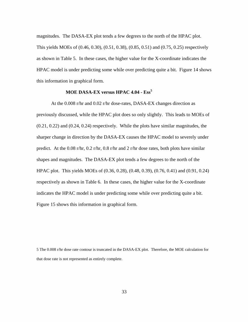
13. Ess, HPAC 4.04 ...........................................................................................................32

14. MOE - Ess, DASA-EX vs. HPAC 4.03 .......................................................................34

15. MOE - Ess, DASA-EX vs. HPAC 4.04 .......................................................................34

16. Operation TEAPOT, Zucchini [DASA-EX, 1979:240]...............................................38

17. Zucchini, DASA-EX....................................................................................................39

18. Zucchini, HPAC 4.03...................................................................................................39

19. Zucchini, HPAC 4.04...................................................................................................39

20. MOE - Zucchini, DASA-EX vs. HPAC 4.03 ..............................................................42

ix

21. MOE - Zucchini, DASA-EX vs. HPAC 4.04 ..............................................................42

22. Operation PLUMBOB, Priscilla [DASA-EX, 1979:276]............................................44

23. Priscilla, DASA-EX.....................................................................................................46

24. Priscilla, HPAC 4.03....................................................................................................46

25. Priscilla, HPAC 4.04....................................................................................................46

26. MOE - Priscilla, DASA-EX vs. HPAC 4.03 ...............................................................49

27. MOE - Priscilla, DASA-EX vs. HPAC 4.04 ...............................................................49

28. Operation PLUMBOB, Smoky [DASA-EX, 1979:328]..............................................52

29. Smoky, DASA-EX.......................................................................................................54

30. Smoky, HPAC 4.03......................................................................................................54

31. Smoky, HPAC 4.04......................................................................................................54

32. MOE - Smoky, DASA-EX vs. HPAC 4.03 .................................................................56

33. MOE - Smoky, DASA-EX vs. HPAC 4.04 .................................................................56

34. Operation SUNBEAM, Johnie Boy [DASA-EX, 1979:565].......................................59

35. Johnie Boy, DASA-EX................................................................................................61

36. Johnie Boy, HPAC 4.03...............................................................................................61

37. Johnie Boy, HPAC 4.04...............................................................................................61

38. MOE - Johnie Boy, DASA-EX vs. HPAC 4.03 ..........................................................64

39. MOE - Johnie Boy, DASA-EX vs. HPAC 4.04 ..........................................................64

40. Example of a Complete Profile File.............................................................................77

x

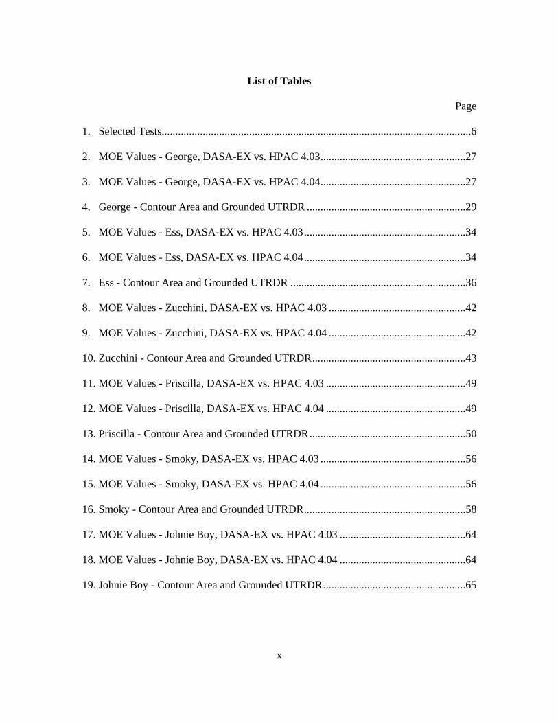
List of Tables

Page

1. Selected Tests.................................................................................................................6

2. MOE Values - George, DASA-EX vs. HPAC 4.03.....................................................27

3. MOE Values - George, DASA-EX vs. HPAC 4.04.....................................................27

4. George - Contour Area and Grounded UTRDR ..........................................................29

5. MOE Values - Ess, DASA-EX vs. HPAC 4.03...........................................................34

6. MOE Values - Ess, DASA-EX vs. HPAC 4.04...........................................................34

7. Ess - Contour Area and Grounded UTRDR ................................................................36

8. MOE Values - Zucchini, DASA-EX vs. HPAC 4.03 ..................................................42

9. MOE Values - Zucchini, DASA-EX vs. HPAC 4.04 ..................................................42

10. Zucchini - Contour Area and Grounded UTRDR........................................................43

11. MOE Values - Priscilla, DASA-EX vs. HPAC 4.03 ...................................................49

12. MOE Values - Priscilla, DASA-EX vs. HPAC 4.04 ...................................................49

13. Priscilla - Contour Area and Grounded UTRDR.........................................................50

14. MOE Values - Smoky, DASA-EX vs. HPAC 4.03 .....................................................56

15. MOE Values - Smoky, DASA-EX vs. HPAC 4.04 .....................................................56

16. Smoky - Contour Area and Grounded UTRDR...........................................................58

17. MOE Values - Johnie Boy, DASA-EX vs. HPAC 4.03 ..............................................64

18. MOE Values - Johnie Boy, DASA-EX vs. HPAC 4.04 ..............................................64

19. Johnie Boy - Contour Area and Grounded UTRDR....................................................65

1



I. Introduction

Motivation

In the event of a nuclear detonation today, especially a terrorist attack on the

continental United States, officials and planners at all levels of government and non-

governmental agencies need the ability to effectively predict fallout patterns and the

ability to provide adequate warning or preparation to civilian populations or military

forces.

The United States last conducted atmospheric nuclear tests in 1962. Data were

collected and reported for each test including wind speed and direction as well as

resulting fallout patterns and doses. Since then, predictions regarding atmospheric

nuclear detonations have been limited to the results of computer modeling and simulation

involving wind transport of radioactive particles and resulting fallout. One such

computer model is Hazard Prediction and Assessment Capability (HPAC) from the

Defense Threat Reduction Agency (DTRA). HPAC predicts hazards based on nuclear,

biological, or chemical event effects. It includes the capability to model effects of

nuclear weapon detonations including fallout and dose rates over geographical areas.

DTRA, particularly the Fallout Working Group, and the Air Force Technical

Applications Center are interested in the independent comparison of HPAC hazard

2

predictions with the actual test data last obtained in 1962. Some visual comparisons have

been done by McGahan [McGahan, 2004]; however, no numerical comparisons have

been accomplished.

Background

Fallout data from test detonations are obtained from “Compilation of Local

Fallout Data from Test Detonations 1945-1962 Extracted from DASA 1251, Volume I -

Continental U.S. Tests” published in 1979 for the Defense Nuclear Agency (DNA),

henceforth referred to as DASA-EX [DASA-EX, 1979:2]. This compilation was

extracted from DASA 1251 “Local fallout from Nuclear Test Detonations” (U)

Volume 2 “Compilation of Fallout Patterns and Related Test Data” (U) Parts 1

through 3. DASA-EX was prepared to serve as an unclassified source of information and

data concerning the atmospheric nuclear test program conducted by the United States

prior to 1963. Data from most U.S. detonations is presented in chronological order,

including fallout patterns for each event. Over time, the Defense Atomic Support

Agency (DASA) became DNA, which became DTRA.

Problem

The focus of this research is to compare the off-site dose-rate contour plots of

select U.S. tests from the 1950s and 1960s produced by HPAC 4.03 and 4.04 with those

found in DASA-EX using test day wind data and additional wind data for up to seven

days following each test. The comparison will be accomplished visually and

numerically. The visual comparison will focus on the magnitude and direction of the

plots. The numerical comparison will use Warner and Platt [Warner, et al, 2001:1] to

3

provide a Measure of Effectiveness (MOE), Rowland and Thompson [Rowland and

Thompson, 1972:5] to provide a Figure of Merit (FM), dose-rate contour area

comparisons and a step-function integration of the dose-rate plots to compare grounded

unit time reference dose rates for each plot.

Scope

The goal is to conduct a comparison of HPAC 4.03 and 4.04 output to off-site

dose-rate contour plots obtained from DASA-EX. A visual comparison of the magnitude

and direction of the plots is conducted. A numerical comparison using Warner and Platt

[Warner, et al, 2001:1], Rowland and Thompson [Rowland and Thompson, 1972:5],

dose-rate contour area comparisons and grounded unit time reference dose rate is also

conducted. The dose-rate contour plots obtained from DASA-EX serve as the only

source of observed, or known, data for this thesis. The contour plots generated by

HPAC 4.03 and 4.04 serve as the prediction.

Approach

DASA-EX was the source of the off-site dose-rate contour plots used to compare

to the HPAC generated plots. Six tests were selected for comparison. Four came from a

list identified by the Fallout Working Group [DTRA, July 2003:12] with the remaining

two chosen by this author. Test day winds data used by the HPAC software were

obtained from “Nuclear Cloud Rise and Growth” [Jodoin, 1994:35]. Additional wind

data for up to seven days following each test were obtained from the Air Force Combat

Climatology Center (AFCCC). Nuclear test information including date, time, yield,

height of burst, latitude and longitude was obtained from DASA-EX. The dose-rate

4

contour plots were generated by HPAC 4.03 and 4.04 and the results were extrapolated to

H+1 hour using the 1.2t− decay approximation [Bridgman, 2001:424]1.

HPAC version 4.03 uses the Defense Land Fallout Interpretive Code (DELFIC)

distribution, a single lognormal distribution, to characterize the distribution of particle

sizes in the fallout ranging from 1-1000 microns. HPAC version 4.04 uses the Heft

distribution [McGahan, October, 2004:1]. It is comprised of a linear combination of

three lognormal distributions, glass, crystalline and local, to characterize the distribution

of particle sizes in the fallout [Heft, 1970:254]. The size of the aerial cloud particles,

which are the glass and crystalline particles, ranges from a few tenths of a micron to one

centimeter. The size of the local particles ranges from tens of microns to several

centimeters [Heft, 1970:256]. Plots of these two distributions (DELFIC and Heft) can be

found in Skaar [Skaar, 2005].

The resulting fallout plots provide a direct visual comparison, giving the reader a

sense of the magnitude and direction of the HPAC predictive plots compared to the

DASA-EX actual plots. The actual and predictive plots were then discretized to provide

a point-wise numerical comparison of regions of overlap and exclusion between the two

plots to provide a MOE and FM. The dose-rate contour areas were then compared. The

plots were then evaluated using step-function integration to provide a comparison of unit

time reference dose rates.

1 The 1.2t− law was used because this is the same adjustment used by DASA-EX to adjust later time

measurements to an H+1 hour dose rate for the tests researched.

5

Sequence of Presentation

Chapter 2 presents the methodology of this research effort including discussions

of the HPAC software, DASA-EX, selected U.S. atmospheric nuclear tests, procedure,

MOE, FM, dose-rate contour area comparison and grounded unit time reference dose

rate. Chapter 3 presents visual and numerical comparisons of HPAC predictions. The

HPAC predictions used the data from DASA-EX, Jodoin, AFCCC and the actual dose-

rate contour plots from DASA-EX. Chapter 4 presents a summary of the results and

provides recommendations for future endeavors in this topic of research. Appendix A

contains an example of the process. Appendix B contains a sample weather profile for a

test.

6

II. Methodology

Chapter Overview

The purpose of this chapter is to present the methodology of this research effort

including discussions of the selected U.S. atmospheric nuclear tests, procedure, HPAC

software, DASA-EX, MOE, FM dose-rate contour area comparison and grounded unit

time reference dose rate.

Selected Tests

Six tests were selected for this research effort. Two, George and Zucchini, were

randomly selected by this author and four were selected from a list identified by the

Fallout Working Group, chaired by DTRA [DTRA, July 2003:12]. The tests are

identified in Table 1.

Table 1. Selected Tests

OPERATION TEST DATE/TIME (Z) YIELD (kT) HEIGHT OF BURST (ft)

TUMBLER-SNAPPER George 1 Jun 52/1155Z 15 300

TEAPOT Ess 23 Mar 55/2030Z 1 -67

TEAPOT Zucchini 15 May 55/1200Z 28 500

PLUMBOB Priscilla 24 Jun 57/1330Z 37 700

PLUMBOB Smoky 31 Aug 57/1230Z 44 700

SUNBEAM Johnie Boy 11 Jul 62/1645Z 0.5 -2

Each test was checked to ensure the detonation was below the fallout-free height

of burst [Glasstone and Dolan, 1977:71]. A detonation below this height can be assumed

7

to generate appreciable or significant fallout. A detonation above this height will still

produce fallout, but local fallout will be negligible compared to a burst where the fireball

touches the ground. The fallout free height of burst is found using Equation (1)

0.4180H W≈ (1)

where H is the maximum height of burst for which there will be appreciable fallout and

W is the actual yield in kilotons [Glasstone and Dolan, 1977:71].

Test information was input into both versions of HPAC to produce dose-rate

contour plots for comparison with those found in DASA-EX. The HPAC plots were

visually compared to those found in DASA-EX with emphasis on magnitude and

direction of the plots. The plots were also compared numerically using two comparative

methods. One method is the Measure of Effectiveness which involves point-to-point

comparisons. This method is described by Warner, et al. The other method is the Figure

of Merit which is an areal comparison developed by Rowland and Thompson.

Additionally, an areal comparison of the individual dose-rate contours was performed.

Finally, a step-function integration of each plot was performed to allow a comparison of

total activity between the three plots. This integration is an approximation of the unit

time reference dose rate which will be defined later in this chapter.

HPAC Overview

HPAC software is a counterproliferation and counterforce tool designed to predict

the effects of chemical, biological, radiological and nuclear (CBRN) events including

releases into the atmosphere and the corresponding effects on civilian and military

populations. War fighters can use HPAC to weaponeer targets containing weapons of

8

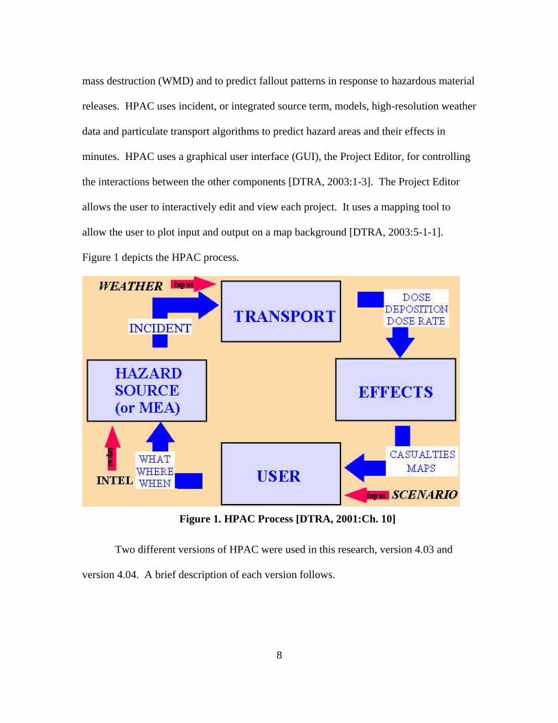
mass destruction (WMD) and to predict fallout patterns in response to hazardous material

releases. HPAC uses incident, or integrated source term, models, high-resolution weather

data and particulate transport algorithms to predict hazard areas and their effects in

minutes. HPAC uses a graphical user interface (GUI), the Project Editor, for controlling

the interactions between the other components [DTRA, 2003:1-3]. The Project Editor

allows the user to interactively edit and view each project. It uses a mapping tool to

allow the user to plot input and output on a map background [DTRA, 2003:5-1-1].

Figure 1 depicts the HPAC process.

Figure 1. HPAC Process [DTRA, 2001:Ch. 10]

Two different versions of HPAC were used in this research, version 4.03 and

version 4.04. A brief description of each version follows.

9

HPAC 4.03 and the DELFIC Particle Size Distribution

HPAC 4.03 uses one of seven integrated incident models, or source term models,

to calculate the associated CBRN material release based on the user’s input. The source

term model used for this research effort was the Nuclear Weapon Explosion (NWPN)

model [DTRA, 2003:1-3]. The NWPN model supports three types of nuclear weapons:

surface or low-air burst (standard), buried and “special.” The special weapon type is

intended for low-yield weapons detonated within a structure and is not applicable to this

research effort [DTRA, 2003:6-5-1]. NWPN defaults to U-238 as the fissionable material

for all three weapon types. The NWPN model determines the amount and distribution of

radioactive particles for HPAC to transport. It uses the DELFIC cloud rise model, using

a weather profile provided by HPAC to generate the cloud rise in the spatial and temporal

domains. When the cloud height stabilizes, DELFIC passes the activity distribution to

HPAC for the transport process [DTRA, 2003:6-5-1].

The cloud activity distributions are based on the legacy fallout codes NewFall and

K-Division Fallout Code, version 3 (KDFOC3) [DTRA, 2003:6-5-1]. These routines

prescribe both activity and dust lofting by particle size group. NewFall uses the DELFIC

distribution, a single lognormal distribution, to characterize the distribution of particle

sizes in the fallout ranging from 1-1000 microns. NWPN uses KDFOC3 to prescribe

both activity and dust lofting by particle size group for buried weapons [DTRA,

2003:6-5-1]. KDFOC3 breaks the nuclear detonation cloud in to three separate clouds:

the mushroom, the stem and the base surge. KDFOC3 maintains two log-normal particle

distributions for each cloud [DTRA, 2003:H-5].

10

HPAC 4.04 and the Heft Particle Size Distribution

HPAC 4.04 uses one of twelve integrated incident models, or source term models,

to calculate the associated CBRN material release based on the user’s input. The source

term model used for this research effort was the Nuclear Weapon Special Edition

(NWPNSE) model [DTRA, 2004:422]. The NWPNSE model supports three types of

nuclear weapons: surface or low-air burst (standard), buried and contained. As with

HPAC 4.03, the contained weapon type is not applicable to this research effort. Like the

NWPN model in HPAC 4.03, NWPNSE defaults to U-238 as the fissionable material for

all three weapon types. The NWPNSE model determines the amount and distribution of

radioactive particles for HPAC to transport. It uses the DELFIC cloud rise model, using

a weather profile provided by HPAC to generate the cloud rise in the spatial and temporal

domains [DTRA, 2004:424]. However, cloud activity distributions are based on the Heft

distribution. It is comprised of a linear combination of three lognormal distributions,

glass, crystalline and local, to characterize the distribution of particle sizes in the fallout

[Heft, 1970:254] [Skaar, 2005].

The crystalline particles are comprised of local soil material that was not melted

due to entering the fireball at a late time [Heft, 1970:255]. The particle densities match

those of the local soil. The glass particles are those particles that entered the fireball

earlier and were therefore subjected to more heat. They are more abundant and typically

have a larger particle diameter than the population of crystalline particles [Heft,

1970:255]. The glass particle densities are slightly less than or equal to the local soil.

The diameter of the aerial cloud particles, comprised of the glass and crystalline particles,

11

ranges from a few tenths of a micron to one centimeter [Heft, 1970:256]. The third

component of the Heft distribution is the local distribution. These particles are a result of

soil material interacting with the fireball at high temperature but separating from the

fireball, before the temperature falls below the melting point of the soil. The local

particle densities are usually very low compared to the local soil. The diameter of the

local particles ranges from tens of microns to several centimeters [Heft, 1970:256].

HPAC Weather and Terrain

HPAC then uses its integrated databases that provide environmental data

including weather and terrain and routines. These databases also interact with the user’s

weather data files that are downloaded from a Meteorological Data Server or other

external data sources. The external data are more applicable to the user’s particular

incident of interest and therefore produce more tailored results. HPAC automatically

invokes a mass-consistent wind field model called the Stationary WInd Fit and

Turbulence (SWIFT) model when terrain elevation data are used [DTRA, 2003:1-3].

Weather is a key factor in predicting the downwind hazard associated with a

particular release of weapons of mass destruction. Key variables include wind speed and

direction, temperature, and humidity. These variables are critical in determining the

direction and distribution of hazardous material. HPAC includes at least five different

methods for getting weather data into the atmospheric transport model known as

SCIPUFF. The methods are: fixed winds; historical weather data or climatology; surface

observations and upper air profiles; mass consistent wind fields; and prognostic

numerical weather prediction model output in either gridded or profile format [DTRA,

12

2003:4-9]. This author used upper air profiles to provide weather data. Detailed

information on upper air profiles can be found in Appendix B: Weather Profiles.

The weather profiles used for this research effort are from two sources. Jodoin’s

dissertation [Jodoin, 1994:38] was the source of initial weather data, obtained as close to

the detonation time and location as possible. Weather data for the seven days following

the test were also obtained from the Air Force Combat Climatology Center (AFCCC).

These data contained multiple updates for up to three different observation stations in the

region of the test. In both cases, the weather data included wind direction, wind speed,

pressure, temperature and humidity at different altitudes. Detailed information on these

profiles is in Appendix B: Weather Profiles.

HPAC uses two types of terrain data. The default assumption is a flat Earth for

the terrain, used to approximate small spatial domains. The second option uses a

complex option. It uses 3-D terrain data representing topographic variations. However,

use of the complex terrain option automatically invokes the mass-consistent wind field

model, SWIFT [DTRA, 2003:4-10]. This research used the flat Earth assumption.

HPAC Transport

HPAC then uses its particulate transport algorithms called the Second-order

Closure Integrated PUFF (SCIPUFF) model. SCIPUFF is a Lagrangian model that

calculates material dispersion in the environment, taking into account diffusion and

turbulence caused by weather, terrain and other factors [Sykes, 1998:1]. Two noteworthy

aspects of the SCIPUFF model are the numerical technique used to solve the dispersion

model and the parameter used for turbulent diffusion. Gaussian puff methodology is used

13

to numerically solve the dispersion model equations. In this method, a collection of

arbitrarily oriented three-dimensional puffs is used to represent a time-dependent

concentration field, which is also arbitrary. Second order closure theory is used to

parameterize the turbulent diffusion, linking the atmospheric wind velocity statistics and

predicted dispersion rates of lofted materials [Sykes, 1998:1].

DASA-EX Test Data

DASA-EX was prepared by General Electric in 1979 for DNA to serve as an

unclassified source of information and data regarding the atmospheric nuclear tests

conducted by the U.S. prior to 1963. Data from most U.S. detonations are presented in

chronological order, including fallout patterns for each event [DASA-EX:2].

DASA-EX includes basic data for each test such as date, time, latitude, longitude,

height of burst in feet and yield in kilotons. Wind speed and direction as a function of

altitude are included for each test. The data are for times as close to the test time as

possible. The wind direction is given in degrees from where the wind is blowing,

measured clockwise from the north. Wind velocities listed are in statute miles per hour.

On-site and off-site fallout patterns with dose-rate contours are included for most

tests. The dose-rate contours were drawn to show gamma dose rate in roentgens per

hour, three feet above the ground at one hour past detonation reference time. When no

actual decay information was available, the 1.2t− decay approximation was used to

extrapolate the data to H+1 hour [DASA-EX:2].

14

Measure of Effectiveness, Warner, et al

This numerical comparison looks at areas of dose-rate contours for each type of

plot and compares them on a point by point basis. In this case, the plots from DASA-EX

are compared with the plots from HPAC versions 4.03 and 4.04. The dose-rate contour

plots from DASA-EX are defined as the areas of observation. The dose-rate contour

plots from both versions of HPAC are defined as the areas of prediction. Areas where

DASA-EX and each version of HPAC agree are defined as areas of overlap. Areas

attributed solely to DASA-EX with no overlap from HPAC are defined as areas of false

negative. That is to say, there are observed data from DASA-EX, but no prediction from

HPAC to match the data. Areas attributed solely to HPAC with no overlap from

DASA-EX are defined as areas of false positive. In this case, there are no observed data

from DASA-EX, yet HPAC predicted the area [Warner, et al, 2001:1]. Figure 2

illustrates the different types of area definitions.

Figure 2. Conceptual View of 3 Comparative Dimensions [Warner, et al, 2001:1]

This Measure of Effectiveness (MOE) is a two-dimensional comparison. The

x-axis of the comparison is composed of the ratio of overlap to the observed area. The

y-axis of the comparison is composed of the ratio of overlap to the predicted area

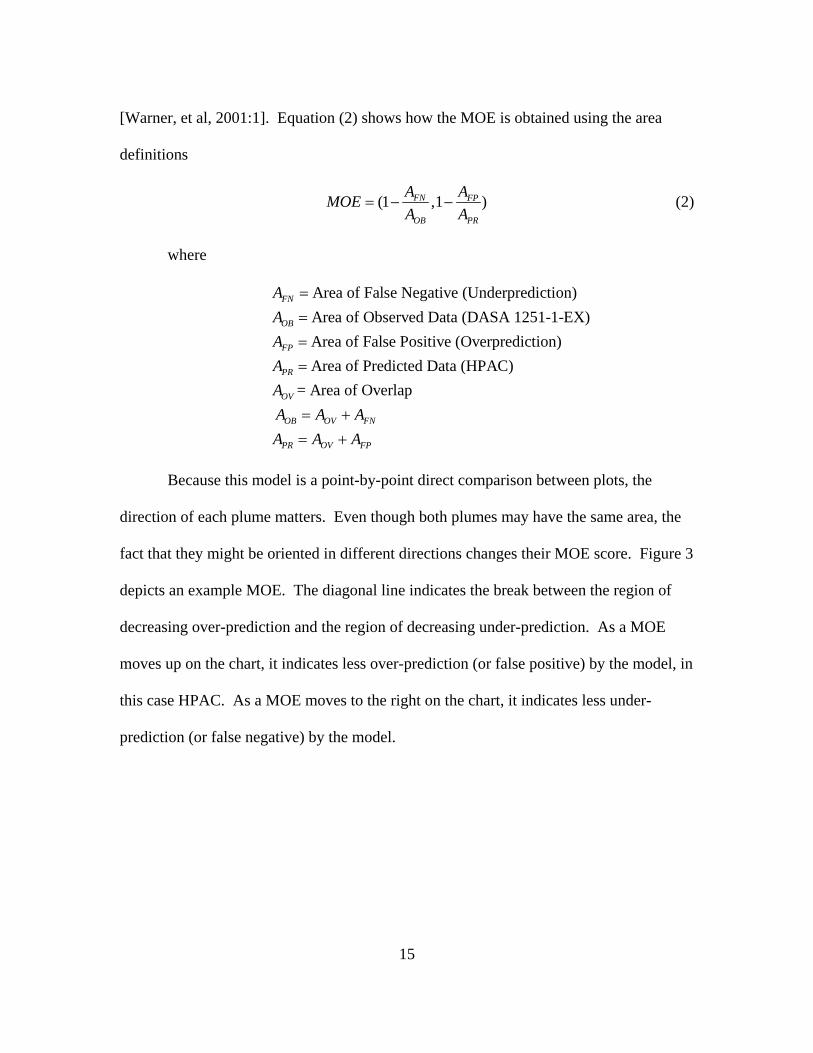
15

[Warner, et al, 2001:1]. Equation (2) shows how the MOE is obtained using the area

definitions

(1 ,1 )FN FP

OB PR

A AMOEA A

= − − (2)

where

Area of False Negative (Underprediction)Area of Observed Data (DASA 1251-1-EX)Area of False Positive (Overprediction)Area of Predicted Data (HPAC)

= Area of Overlap

FN

OB

FP

PR

OV

OB OV FN

PR O

AAAAAA A AA A

=

===

= +

= V FPA+

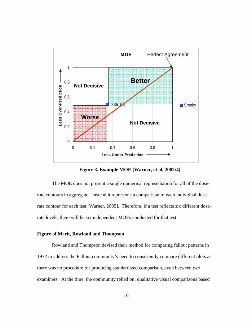
Because this model is a point-by-point direct comparison between plots, the

direction of each plume matters. Even though both plumes may have the same area, the

fact that they might be oriented in different directions changes their MOE score. Figure 3

depicts an example MOE. The diagonal line indicates the break between the region of

decreasing over-prediction and the region of decreasing under-prediction. As a MOE

moves up on the chart, it indicates less over-prediction (or false positive) by the model, in

this case HPAC. As a MOE moves to the right on the chart, it indicates less under-

prediction (or false negative) by the model.

16

Figure 3. Example MOE [Warner, et al, 2002:4]

The MOE does not present a single numerical representation for all of the dose-

rate contours in aggregate. Instead it represents a comparison of each individual dose-

rate contour for each test [Warner, 2005]. Therefore, if a test reflects six different dose-

rate levels, there will be six independent MOEs conducted for that test.

Figure of Merit, Rowland and Thompson

Rowland and Thompson devised their method for comparing fallout patterns in

1972 to address the Fallout community’s need to consistently compare different plots as

there was no procedure for producing standardized comparison, even between two

examiners. At the time, the community relied on: qualitative visual comparisons based

MOE

0.35, 0.5

0

0.2

0.4

0.6

0.8

1

0 0.2 0.4 0.6 0.8 1

Less Under-Prediction

Less

Ove

r-Pre

dict

ion

Smoky

Perfect Agreement

Better

Worse

Not Decisive

Not Decisive

17

on juxtaposition of contour plots reduced to similar scales; hotline comparisons involving

greatest radial extent of a particular dose rate and widths of contours at certain distances;

areal measurements of specific contours and cumulative doses compared to radial

distances; and exact measurements involving point-to-point comparisons within the

contour plots [Rowland and Thompson, 1972:3].

The visual comparisons were sensitive to observer bias while the hotline

comparisons had multiple trade-offs at each area of comparison such as deciding the

merit of shorter or longer radial distances compared to wider or narrower contours. Areal

comparisons by separate contour did not produce an integrated measure. At the time,

exact, point-to-point comparisons were not a viable option [Rowland and Thompson,

1972:4].

Their method is based on the areal method and derives a single Figure of

Merit (FM) to numerically quantify the goodness of fit between two fallout patterns.

Their FM accounts for the areal distribution of the contour plots, the dose-rate of each

contour and direction of each contour plot. The area of each similar contour pattern

being compared is calculated and the area which does not overlap for the same two

contour plots is also calculated. The measure of agreement is given by a non-linear FM

ranging from 0, no common area, to 1, two identical patterns [Rowland and Thompson,

1972:5]. Equation (3) shows how the FM is obtained.

18

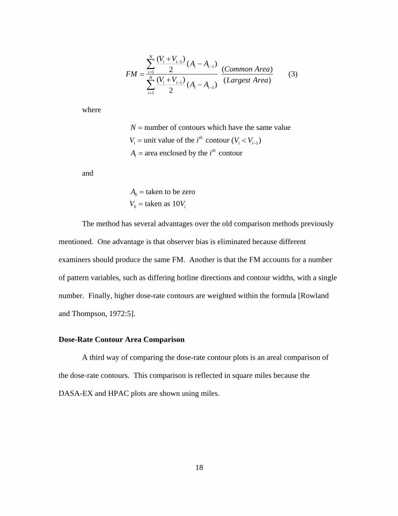
11

1

11

1

( ) ( )( )2

( ) ( )( )2

Ni i

i iiN

i ii i

i

V V A ACommon AreaFM

V V Largest AreaA A

−−

=

−−

=

+−

=

+ −

∑

∑ (3)

where

1

number of contours which have the same valueunit value of the contour ( )

area enclosed by the contour

thi i i

thi

NV i V V

A i−

=

= <

=

and

0

0

taken to be zerotaken as 10 i

AV V

==

The method has several advantages over the old comparison methods previously

mentioned. One advantage is that observer bias is eliminated because different

examiners should produce the same FM. Another is that the FM accounts for a number

of pattern variables, such as differing hotline directions and contour widths, with a single

number. Finally, higher dose-rate contours are weighted within the formula [Rowland

and Thompson, 1972:5].

Dose-Rate Contour Area Comparison

A third way of comparing the dose-rate contour plots is an areal comparison of

the dose-rate contours. This comparison is reflected in square miles because the

DASA-EX and HPAC plots are shown using miles.

19

Grounded Unit Time Reference Dose Rate

The final method of numerically comparing the dose-rate contour plots is the unit

time reference dose rate (at one hour) for each plot. The unit time reference dose rate

represents the dose rate if a volumetric integration of the activity remaining in the air and

deposited on the ground were performed at one hour [Bridgman, 2001:425]. Normally,

the unit time reference dose rate would be derived using continuous dose rates radiating

out from ground zero. However, the dose-rate contour plots from DASA-EX represent

only the grounded activity in a step-wise fashion. For this reason, the dose-rate contour

plots from both versions of HPAC were also evaluated in a step-wise fashion. The step-

function integration was performed taking each dose rate value at one hour on a fine grid,

multiplying them by the area that each point represents and summing them all. The sum

was divided by the yield, which then represents the dose rate at one hour per kiloton for

one square kilometer. This sum is a stepwise approximation to the grounded portion of

the unit time reference dose rate, henceforth referred to as Grounded UTRDR. Its value

will always be less than the true unit time reference dose rate.

If all of the activity for one kiloton of fission indicated by the volumetric

integration mentioned above were spread uniformly over one square kilometer at one

hour, the total activity would be called the source normalization constant, as derived by

Bridgman [Bridgman, 2001:425]. Expected values for the source normalization constant,

k, range between 2590 to over 7500 2R km

hr kT−−

[Bridgman, 2001:436]. This value is based

on 75% of the total gamma activity attributed by Glasstone and Dolan to the fission

products produced by one kiloton of fission, 530 gamma-megacuries at one hour after

20

detonation [Glasstone and Dolan, 1977:453]. The fraction 75 percent is based in part on

Baker’s bimodal distribution which assumes 75 percent of the activity is contained in the

particles which contribute to local fallout [Bridgman, 2001:425]. Hereafter, this value of

the source normalization constant is referred to as the “theoretical value” and is provided

for comparative purposes only.

21

III. Results and Comparisons

Chapter Overview

The purpose of this chapter is to present visual and numerical comparisons of

HPAC predictions using the data from DASA-EX, Jodoin and AFCCC, and the actual

dose-rate contour plots from DASA-EX. The tests are presented in chronological order,

earliest to latest. Dose-rate contour plots for each test are depicted in four ways in this

chapter. The plot is presented in its original format from DASA-EX and then in the gray-

scale format which is a product of Canvas software [Canvas 2004]. The Canvas software

was used to import the line drawings from DASA-EX and HPAC and turn them into a

gray scale picture by tracing the drawings and establishing contour plots for each dose

rate within the test.

Dose-rate contour plots from HPAC 4.03 and 4.04 are also presented in gray scale

format. Extra effort was taken to present the plots so that all are on the same scale. This

should give the reader a visual appreciation of the differences in magnitude and direction.

Operation TUMBLER-SNAPPER George

The George test shot took place June 1, 1952 at 1155 Greenwich Mean Time

(GMT) or Zulu (Z). It was a tower burst, detonated 300 feet above the ground, yielding

15 kilotons. The off-site fallout pattern at Figure 4 was drawn from readings obtained by

ground mobile monitors from the Radiological Safety organization on detonation day

(D-Day). Off-site refers to the area exceeding 4000 yards from ground zero [DASA-EX,

1979:93]. The dose-rates were extrapolated to H+1 hour using the 1.2t− decay

approximation [DASA-EX, 1979:93]. The dose-rate contours were plotted on a grid with

22

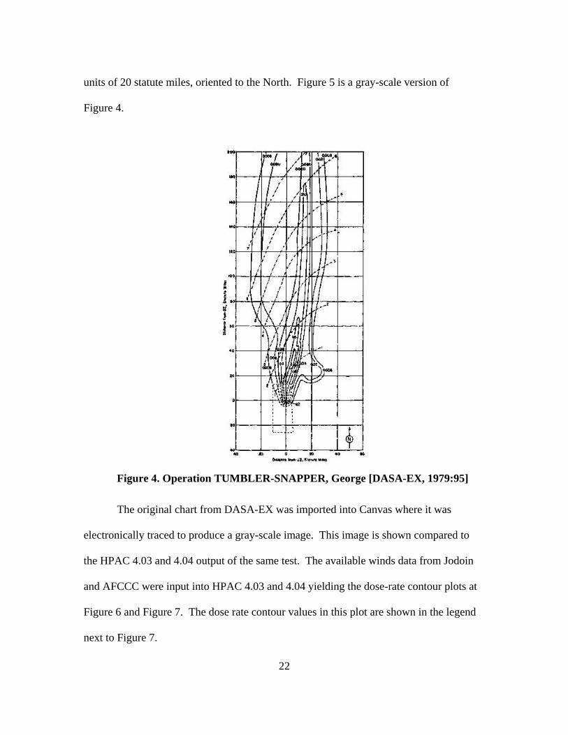
units of 20 statute miles, oriented to the North. Figure 5 is a gray-scale version of

Figure 4.

Figure 4. Operation TUMBLER-SNAPPER, George [DASA-EX, 1979:95]

The original chart from DASA-EX was imported into Canvas where it was

electronically traced to produce a gray-scale image. This image is shown compared to

the HPAC 4.03 and 4.04 output of the same test. The available winds data from Jodoin

and AFCCC were input into HPAC 4.03 and 4.04 yielding the dose-rate contour plots at

Figure 6 and Figure 7. The dose rate contour values in this plot are shown in the legend

next to Figure 7.

23

Visual Comparison - George

A visual comparison of Figure 5, Figure 6 and Figure 7 indicates all three plots

are oriented in the same northerly direction. The rough magnitudes of all three plots are

the same; all extend at least 200 miles. The DASA-EX plot and the HPAC 4.03 plots are

at least 60 miles wide, while the HPAC 4.04 plot is narrower, measuring approximately

40 miles wide. The DASA-EX plot shows some unique features in the 0.008 r/hr and

0.02 r/hr dose-rate contour plots at the lower southeast corner and along the lower

western side. The spur in the southeast corner and the exaggerated bulge in the lower

western side are not modeled in either of the HPAC plots, although there is a slight curve

to the west in the HPAC plots for the corresponding dose-rate contour plots at the

location of the exaggerated bulge in the DASA-EX plot. These unique features could be

due to terrain features not adequately modeled in either version of HPAC or limitations in

the sampling techniques at the time of the test. The dose-rate contour plots for 0.08 r/hr

and higher are significantly narrower in the DASA-EX plot as compared to both of the

HPAC plots. Again, this could be terrain dependent, sampling technique or an artifact of

the modeling techniques reflected in HPAC.

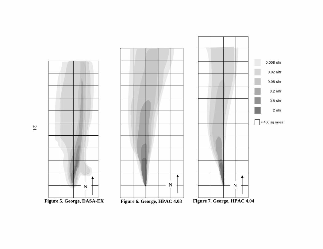
Figure 5. George, DASA-EX

Figure 6. George, HPAC 4.03

Figure 7. George, HPAC 4.04

0.008 r/hr

0.02 r/hr

0.08 r/hr

0.2 r/hr

0.8 r/hr

2 r/hr

= 400 sq miles

N N

24

N

25

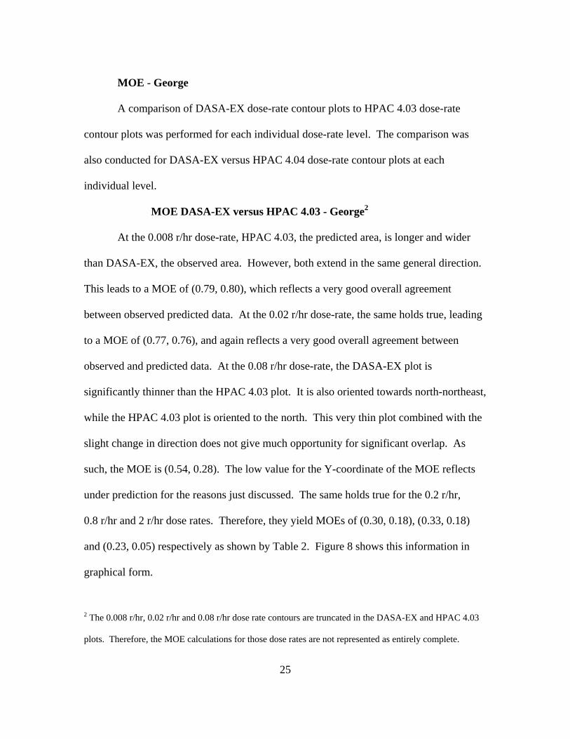
MOE - George

A comparison of DASA-EX dose-rate contour plots to HPAC 4.03 dose-rate

contour plots was performed for each individual dose-rate level. The comparison was

also conducted for DASA-EX versus HPAC 4.04 dose-rate contour plots at each

individual level.

MOE DASA-EX versus HPAC 4.03 - George2

At the 0.008 r/hr dose-rate, HPAC 4.03, the predicted area, is longer and wider

than DASA-EX, the observed area. However, both extend in the same general direction.

This leads to a MOE of (0.79, 0.80), which reflects a very good overall agreement

between observed predicted data. At the 0.02 r/hr dose-rate, the same holds true, leading

to a MOE of (0.77, 0.76), and again reflects a very good overall agreement between

observed and predicted data. At the 0.08 r/hr dose-rate, the DASA-EX plot is

significantly thinner than the HPAC 4.03 plot. It is also oriented towards north-northeast,

while the HPAC 4.03 plot is oriented to the north. This very thin plot combined with the

slight change in direction does not give much opportunity for significant overlap. As

such, the MOE is (0.54, 0.28). The low value for the Y-coordinate of the MOE reflects

under prediction for the reasons just discussed. The same holds true for the 0.2 r/hr,

0.8 r/hr and 2 r/hr dose rates. Therefore, they yield MOEs of (0.30, 0.18), (0.33, 0.18)

and (0.23, 0.05) respectively as shown by Table 2. Figure 8 shows this information in

graphical form.

2 The 0.008 r/hr, 0.02 r/hr and 0.08 r/hr dose rate contours are truncated in the DASA-EX and HPAC 4.03

plots. Therefore, the MOE calculations for those dose rates are not represented as entirely complete.

26

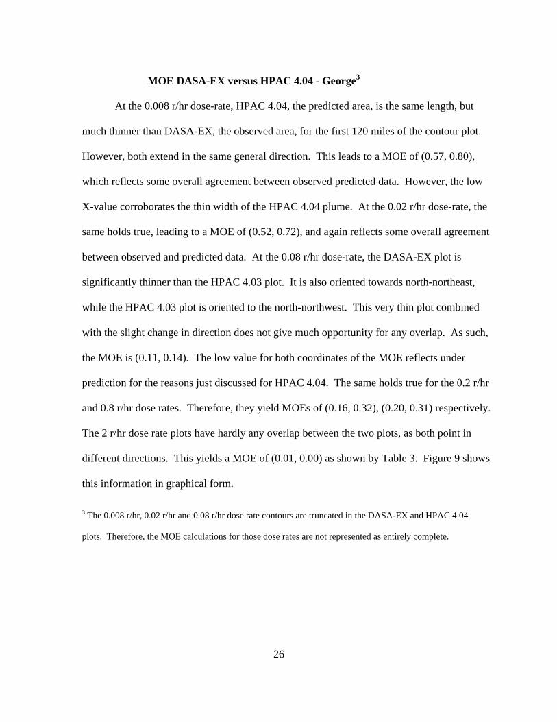
MOE DASA-EX versus HPAC 4.04 - George3

At the 0.008 r/hr dose-rate, HPAC 4.04, the predicted area, is the same length, but

much thinner than DASA-EX, the observed area, for the first 120 miles of the contour plot.

However, both extend in the same general direction. This leads to a MOE of (0.57, 0.80),

which reflects some overall agreement between observed predicted data. However, the low

X-value corroborates the thin width of the HPAC 4.04 plume. At the 0.02 r/hr dose-rate, the

same holds true, leading to a MOE of (0.52, 0.72), and again reflects some overall agreement

between observed and predicted data. At the 0.08 r/hr dose-rate, the DASA-EX plot is

significantly thinner than the HPAC 4.03 plot. It is also oriented towards north-northeast,

while the HPAC 4.03 plot is oriented to the north-northwest. This very thin plot combined

with the slight change in direction does not give much opportunity for any overlap. As such,

the MOE is (0.11, 0.14). The low value for both coordinates of the MOE reflects under

prediction for the reasons just discussed for HPAC 4.04. The same holds true for the 0.2 r/hr

and 0.8 r/hr dose rates. Therefore, they yield MOEs of (0.16, 0.32), (0.20, 0.31) respectively.

The 2 r/hr dose rate plots have hardly any overlap between the two plots, as both point in

different directions. This yields a MOE of (0.01, 0.00) as shown by Table 3. Figure 9 shows

this information in graphical form.

3 The 0.008 r/hr, 0.02 r/hr and 0.08 r/hr dose rate contours are truncated in the DASA-EX and HPAC 4.04

plots. Therefore, the MOE calculations for those dose rates are not represented as entirely complete.

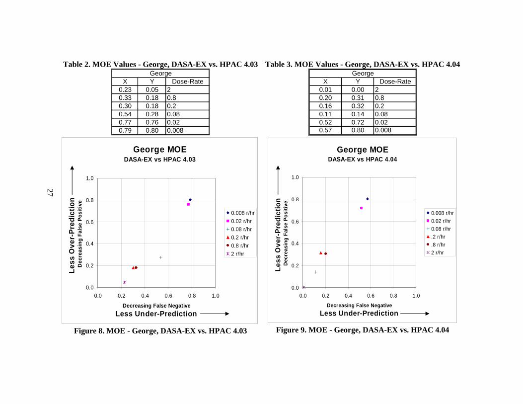
Table 2. MOE Values - George, DASA-EX vs. HPAC 4.03

X Y Dose-Rate0.23 0.05 20.33 0.18 0.80.30 0.18 0.20.54 0.28 0.080.77 0.76 0.020.79 0.80 0.008

George

George MOEDASA-EX vs HPAC 4.03

0.0

0.2

0.4

0.6

0.8

1.0

0.0 0.2 0.4 0.6 0.8 1.0

Decreasing False NegativeLess Under-Prediction

Less

Ove

r-Pr

edic

tion

Dec

reas

ing

Fals

e Po

sitiv

e

0.008 r/hr0.02 r/hr0.08 r/hr0.2 r/hr0.8 r/hr2 r/hr

Figure 8. MOE - George, DASA-EX vs. HPAC 4.03

Table 3. MOE Values - George, DASA-EX vs. HPAC 4.04

X Y Dose-Rate0.01 0.00 20.20 0.31 0.80.16 0.32 0.20.11 0.14 0.080.52 0.72 0.020.57 0.80 0.008

George

George MOEDASA-EX vs HPAC 4.04

0.0

0.2

0.4

0.6

0.8

1.0

0.0 0.2 0.4 0.6 0.8 1.0


Less

Ove

r-Pr

edic

tion

Dec

reas

ing

Fals

e Po

sitiv

e

0.008 r/hr0.02 r/hr0.08 r/hr.2 r/hr.8 r/hr2 r/hr

Figure 9. MOE - George, DASA-EX vs. HPAC 4.04

27

28

FM - George

The non-linear FM for comparing the DASA-EX dose-rate contour plots to those

of HPAC 4.03 is 0.17. The value for the comparison between DASA-EX and

HPAC 4.04 is 0.08. These values are weighted based on the values of the dose-rates.

Therefore, the fact that both of the HPAC plots and the DASA-EX plots diverge at the

higher dose-rates means the FM is low even though the overall magnitude and direction

of the plots are similar as discussed in the visual comparison portion above.

Dose-Rate Contour Area - George

The dose-rate contour areal comparison is summarized in Table 4. The data agree

with the visual comparison previously discussed. HPAC 4.03 predicts larger dose-rate

contour areas with the exception of the 0.02 r/hr dose-rate.

Grounded UTRDR - George

The Grounded UTRDR is summarized in Table 4 in 2R km

hr kT⎡ ⎤−⎢ ⎥−⎣ ⎦

. HPAC 4.03

predicts more grounded activity than DASA-EX or HPAC 4.04.

29

Table 4. George - Contour Area and Grounded UTRDR George

Contour Area (sq miles)Dose Rate (r/hr) DASA-EX HPAC 4.03 HPAC 4.04

2 62.6 266.3 120.20.8 246.7 256.5 74.40.2 810.8 1317.2 353.1

0.08 1278.6 2681.7 1269.50.02 5122.2 2995.7 3497.5

0.008 2369.4 2030.6 1546.8 Grounded UTRDR DASA-EX HPAC 4.03 HPAC 4.04 122.3 223.0 95.7

Operation TEAPOT Ess

The Ess test shot took place March 23, 1955 at 2030 Greenwich Mean Time

(GMT) or Zulu (Z). It was a sub-surface burst, detonated 67 feet below the ground,

yielding 1 kiloton. The off-site fallout pattern at Figure 10 was drawn from ground

survey readings taken by the off-site Radiological Safety organization on detonation day



approximation. The dose-rate contours were plotted on a grid with units of 20 statute

miles, oriented to the North. The dose rate contour values in this plot are shown in the

legend next to Figure 11 which is a gray-scale version of Figure 10.

Again, the original chart from DASA-EX was imported into Canvas where it was

electronically traced to produce a gray-scale image. This image is shown compared to

the HPAC 4.03 and 4.04 output of the same test. As before, the available winds data

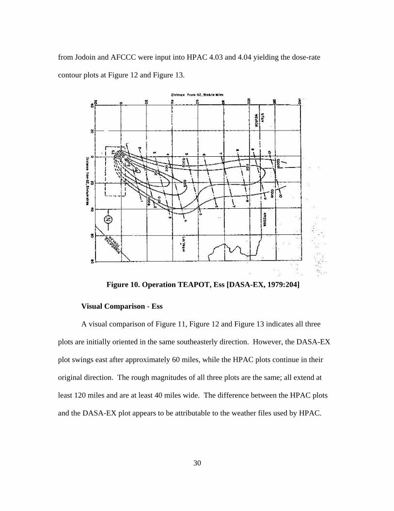
30

from Jodoin and AFCCC were input into HPAC 4.03 and 4.04 yielding the dose-rate

contour plots at Figure 12 and Figure 13.

Figure 10. Operation TEAPOT, Ess [DASA-EX, 1979:204]

Visual Comparison - Ess

A visual comparison of Figure 11, Figure 12 and Figure 13 indicates all three

plots are initially oriented in the same southeasterly direction. However, the DASA-EX

plot swings east after approximately 60 miles, while the HPAC plots continue in their

original direction. The rough magnitudes of all three plots are the same; all extend at

least 120 miles and are at least 40 miles wide. The difference between the HPAC plots

and the DASA-EX plot appears to be attributable to the weather files used by HPAC.

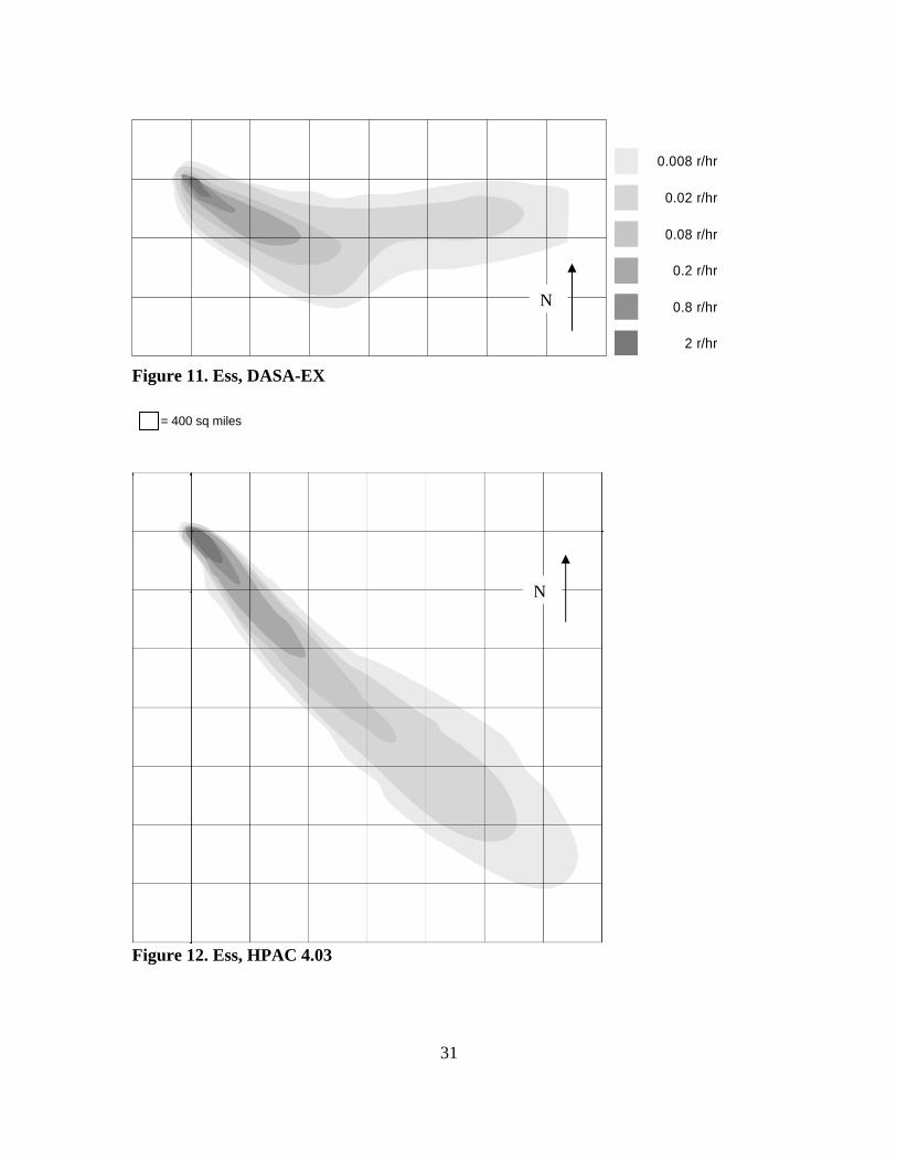
31

0.008 r/hr

0.02 r/hr

0.08 r/hr

0.2 r/hr

0.8 r/hr

2 r/hr Figure 11. Ess, DASA-EX

Figure 12. Ess, HPAC 4.03

= 400 sq miles

N

N

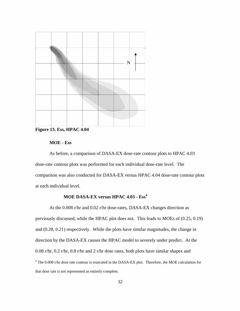
32

Figure 13. Ess, HPAC 4.04

MOE - Ess

As before, a comparison of DASA-EX dose-rate contour plots to HPAC 4.03

dose-rate contour plots was performed for each individual dose-rate level. The

comparison was also conducted for DASA-EX versus HPAC 4.04 dose-rate contour plots

at each individual level.

MOE DASA-EX versus HPAC 4.03 - Ess4

At the 0.008 r/hr and 0.02 r/hr dose-rates, DASA-EX changes direction as

previously discussed, while the HPAC plot does not. This leads to MOEs of (0.25, 0.19)

and (0.28, 0.21) respectively. While the plots have similar magnitudes, the change in

direction by the DASA-EX causes the HPAC model to severely under predict. At the

0.08 r/hr, 0.2 r/hr, 0.8 r/hr and 2 r/hr dose rates, both plots have similar shapes and

4 The 0.008 r/hr dose rate contour is truncated in the DASA-EX plot. Therefore, the MOE calculation for

that dose rate is not represented as entirely complete.

N

33

magnitudes. The DASA-EX plot tends a few degrees to the north of the HPAC plot.

This yields MOEs of (0.46, 0.30), (0.51, 0.38), (0.85, 0.51) and (0.75, 0.25) respectively

as shown in Table 5. In these cases, the higher value for the X-coordinate indicates the

HPAC model is under predicting some while over predicting quite a bit. Figure 14 shows

this information in graphical form.

MOE DASA-EX versus HPAC 4.04 - Ess5

At the 0.008 r/hr and 0.02 r/hr dose-rates, DASA-EX changes direction as

previously discussed, while the HPAC plot does so only slightly. This leads to MOEs of

(0.21, 0.22) and (0.24, 0.24) respectively. While the plots have similar magnitudes, the

sharper change in direction by the DASA-EX causes the HPAC model to severely under

predict. At the 0.08 r/hr, 0.2 r/hr, 0.8 r/hr and 2 r/hr dose rates, both plots have similar

shapes and magnitudes. The DASA-EX plot tends a few degrees to the north of the

HPAC plot. This yields MOEs of (0.36, 0.28), (0.48, 0.39), (0.76, 0.41) and (0.91, 0.24)

respectively as shown in Table 6. In these cases, the higher value for the X-coordinate

indicates the HPAC model is under predicting some while over predicting quite a bit.

Figure 15 shows this information in graphical form.



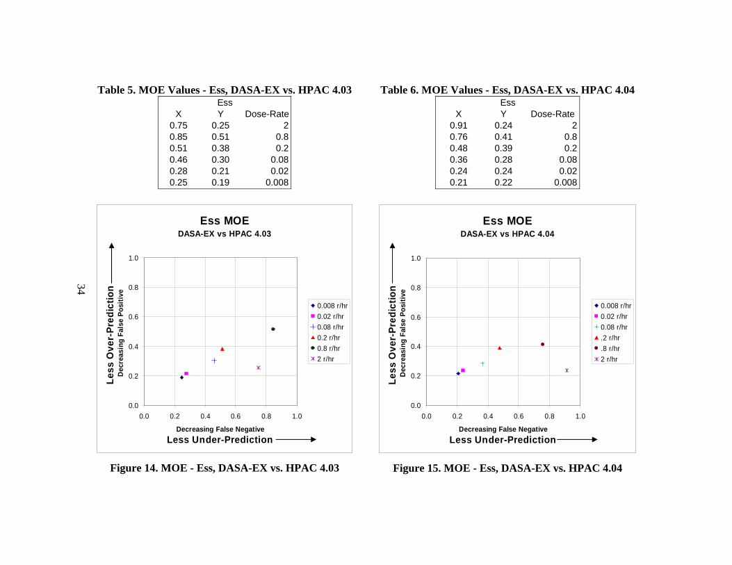
Table 5. MOE Values - Ess, DASA-EX vs. HPAC 4.03

X Y Dose-Rate0.75 0.25 20.85 0.51 0.80.51 0.38 0.20.46 0.30 0.080.28 0.21 0.020.25 0.19 0.008

Ess

Ess MOEDASA-EX vs HPAC 4.03

0.0

0.2

0.4

0.6

0.8

1.0

0.0 0.2 0.4 0.6 0.8 1.0


Less

Ove

r-Pr

edic

tion

Dec

reas

ing

Fals

e Po

sitiv

e


Figure 14. MOE - Ess, DASA-EX vs. HPAC 4.03

Table 6. MOE Values - Ess, DASA-EX vs. HPAC 4.04

X Y Dose-Rate0.91 0.24 20.76 0.41 0.80.48 0.39 0.20.36 0.28 0.080.24 0.24 0.020.21 0.22 0.008

Ess

Ess MOEDASA-EX vs HPAC 4.04

0.0

0.2

0.4

0.6

0.8

1.0

0.0 0.2 0.4 0.6 0.8 1.0


Less

Ove

r-Pr

edic

tion

Dec

reas

ing

Fals

e Po

sitiv

e


Figure 15. MOE - Ess, DASA-EX vs. HPAC 4.04

34

35

FM - Ess



HPAC 4.04 is 0.57. The fact that both of the HPAC plots and the DASA-EX plots

diverge at the lower dose-rates means the FM is somewhat improved because of the

similarities shared at the higher dose rates.

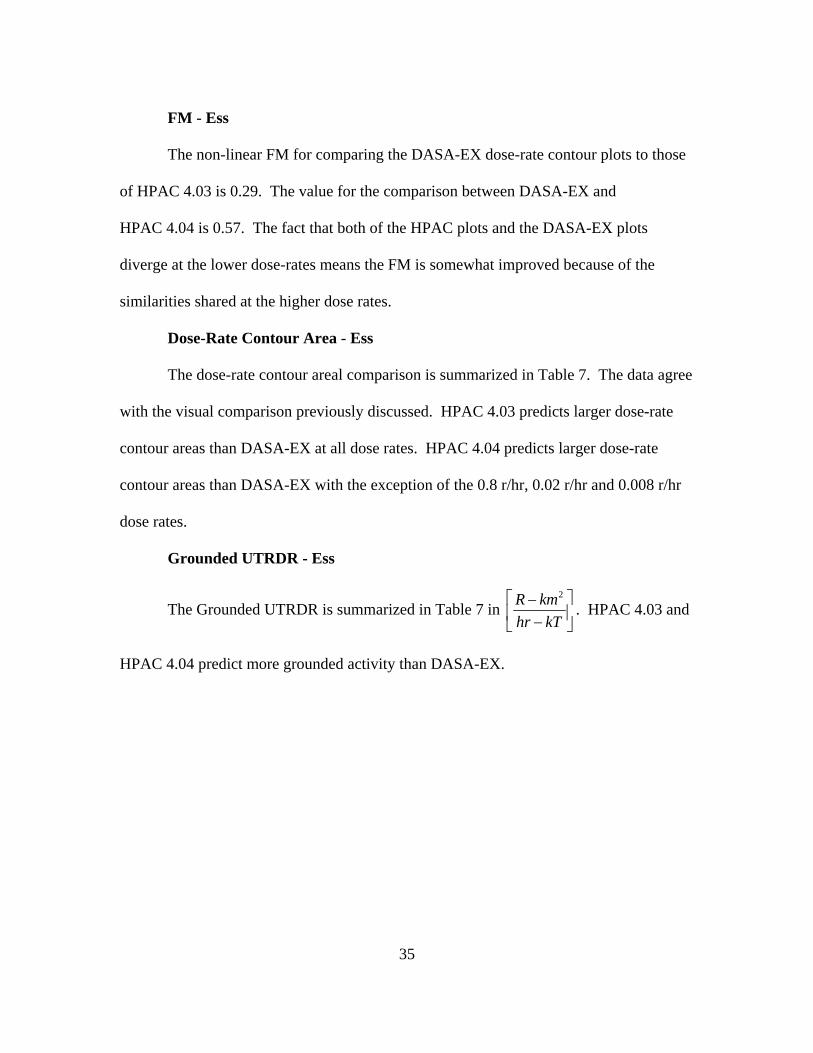
Dose-Rate Contour Area - Ess

The dose-rate contour areal comparison is summarized in Table 7. The data agree

with the visual comparison previously discussed. HPAC 4.03 predicts larger dose-rate

contour areas than DASA-EX at all dose rates. HPAC 4.04 predicts larger dose-rate

contour areas than DASA-EX with the exception of the 0.8 r/hr, 0.02 r/hr and 0.008 r/hr

dose rates.

Grounded UTRDR - Ess


hr kT⎡ ⎤−⎢ ⎥−⎣ ⎦

. HPAC 4.03 and

HPAC 4.04 predict more grounded activity than DASA-EX.

36

Table 7. Ess - Contour Area and Grounded UTRDR Ess

Contour Area (sq miles)Dose Rate DASA-EX HPAC 4.03 HPAC 4.04

2 22.2 58.4 76.5 0.8 52.9 58.2 48.7 0.2 276.5 346.5 303.2

0.08 382.8 606.6 485.3 0.02 1548.7 1794.7 1341.5

0.008 1557.6 2038.5 1335.5 Grounded UTRDR

DASA-EX HPAC 4.03 HPAC 4.04 559.4 862.9 851.7

Operation TEAPOT Zucchini

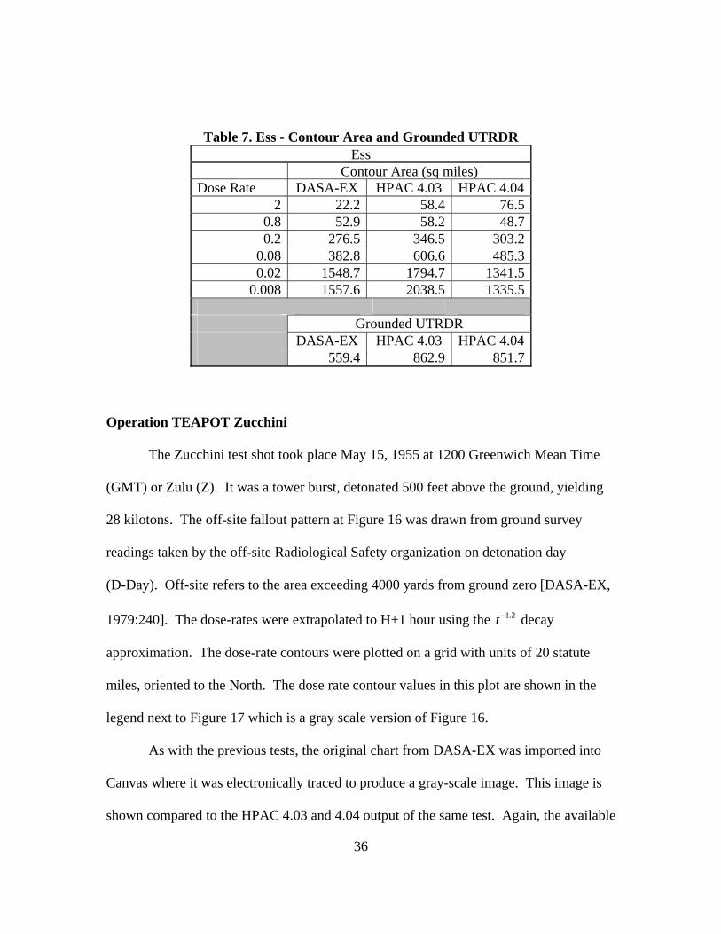
The Zucchini test shot took place May 15, 1955 at 1200 Greenwich Mean Time


28 kilotons. The off-site fallout pattern at Figure 16 was drawn from ground survey

readings taken by the off-site Radiological Safety organization on detonation day





legend next to Figure 17 which is a gray scale version of Figure 16.

As with the previous tests, the original chart from DASA-EX was imported into

Canvas where it was electronically traced to produce a gray-scale image. This image is

shown compared to the HPAC 4.03 and 4.04 output of the same test. Again, the available

37

winds data from Jodoin and AFCCC were input into HPAC 4.03 and 4.04 yielding the

dose-rate contour plots at Figure 18 and Figure 19.

Visual Comparison - Zucchini

A visual comparison of Figure 17, Figure 18 and Figure 19 indicates the HPAC

plots are initially oriented in an easterly direction before swinging to the south east after

approximately 80 miles and then returning to the east after an additional 80 miles.

However, the DASA-EX plot is initially oriented to the southeast before making a hard

swing to the northeast after approximately 60 miles. The magnitudes of the HPAC plots

are much greater than the DASA-EX plot, although the HPAC 4.04 plot is approximately

one third thinner than the HPAC 4.03 plot. The difference between the HPAC plots and

the DASA-EX plot appears to be attributable to the weather files used by HPAC.

Additionally, the DASA-EX plot has a unique indentation on its northwestern edge,

approximately 130 miles from ground zero. It also has at least two pronounced scallops

in its southeastern side starting approximately 100 miles from ground zero. These

features are readily apparent in the HPAC plots and could be due to terrain features not

adequately modeled in either version of HPAC or limitations in the sampling techniques

at the time of the test.

38

Figure 16. Operation TEAPOT, Zucchini [DASA-EX, 1979:240]

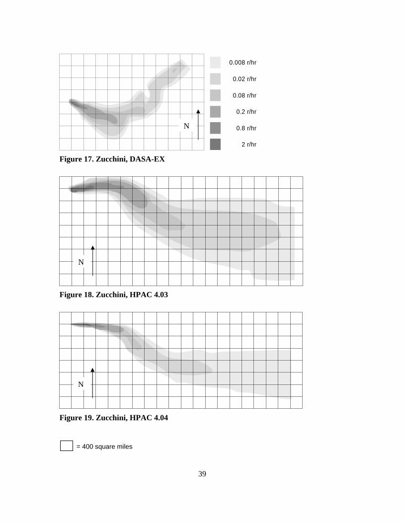
39

0.008 r/hr

0.02 r/hr

0.08 r/hr

0.2 r/hr

0.8 r/hr

2 r/hr Figure 17. Zucchini, DASA-EX

Figure 18. Zucchini, HPAC 4.03

Figure 19. Zucchini, HPAC 4.04

= 400 square miles

N

N

N

40

MOE - Zucchini

Like the previous tests, a comparison of DASA-EX dose-rate contour plots to

HPAC 4.03 dose-rate contour plots was performed for each individual dose-rate level.

The comparison was also conducted for DASA-EX versus HPAC 4.04 dose-rate contour

plots at each individual level.

MOE DASA-EX versus HPAC 4.03 - Zucchini6

In all dose-rate levels except the 2 r/hr, HPAC 4.03 grossly under predicted

compared to the DASA-EX data. This appears to be directly attributable to the dramatic

changes in the contour plots directions typically caused by poor, or incomplete, weather

data. HPAC 4.03 produces dramatically larger plots than DASA-EX; however, they are

oriented in completely different directions. At the 2 r/hr dose rate, there is enough

overlap between the two plots to produce a MOE (0.68, 0.12). The value of the X-

coordinate shows HPAC did not under predict as badly as the remainder of the dose rates.

The MOEs for the lower dose rates are shown in Table 8. Figure 20 shows this

information in graphical form.

6 The 0.008 r/hr and 0.02 r/hr dose rate contours are truncated in the DASA-EX plot and the 0.008 r/hr dose

rate contour is truncated in the HPAC 4.03 plot. Therefore, the MOE calculations for those dose rates are

not represented as entirely complete.

41

MOE DASA-EX versus HPAC 4.04 - Zucchini7

Just like the HPAC 4.03 plots, in all dose-rate levels, HPAC 4.04 grossly under

predicted compared to the DASA-EX data. This appears to be directly attributable to the

dramatic changes in the contour plots directions typically caused by poor, or incomplete,

weather data. HPAC 4.04 produces dramatically larger plots than DASA-EX; however,

they are oriented in completely different directions. The MOEs for all dose rates are

shown in Table 9. Figure 21 shows this information in graphical form.

7 The 0.008 r/hr and 0.02 r/hr dose rate contours are truncated in the DASA-EX plot and the 0.008 r/hr dose

rate contour is truncated in the HPAC 4.04 plot. Therefore, the MOE calculations for those dose rates are

not represented as entirely complete.

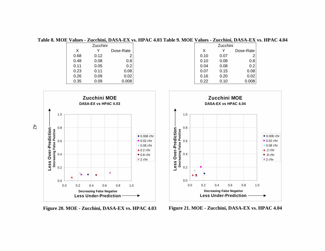
Table 8. MOE Values - Zucchini, DASA-EX vs. HPAC 4.03

X Y Dose-Rate0.68 0.12 20.48 0.08 0.80.11 0.05 0.20.23 0.11 0.080.26 0.09 0.020.35 0.09 0.008

Zucchini

Zucchini MOEDASA-EX vs HPAC 4.03

0.0

0.2

0.4

0.6

0.8

1.0

0.0 0.2 0.4 0.6 0.8 1.0


Less

Ove

r-Pr

edic

tion

Dec

reas

ing

Fals

e Po

sitiv

e


Figure 20. MOE - Zucchini, DASA-EX vs. HPAC 4.03

Table 9. MOE Values - Zucchini, DASA-EX vs. HPAC 4.04

X Y Dose-Rate0.10 0.07 20.10 0.08 0.80.04 0.08 0.20.07 0.15 0.080.16 0.20 0.020.22 0.10 0.008

Zucchini

Zucchini MOEDASA-EX vs HPAC 4.04

0.0

0.2

0.4

0.6

0.8

1.0

0.0 0.2 0.4 0.6 0.8 1.0


Less

Ove

r-Pr

edic

tion

Dec

reas

ing

Fals

e Po

sitiv

e


Figure 21. MOE - Zucchini, DASA-EX vs. HPAC 4.04

42

43

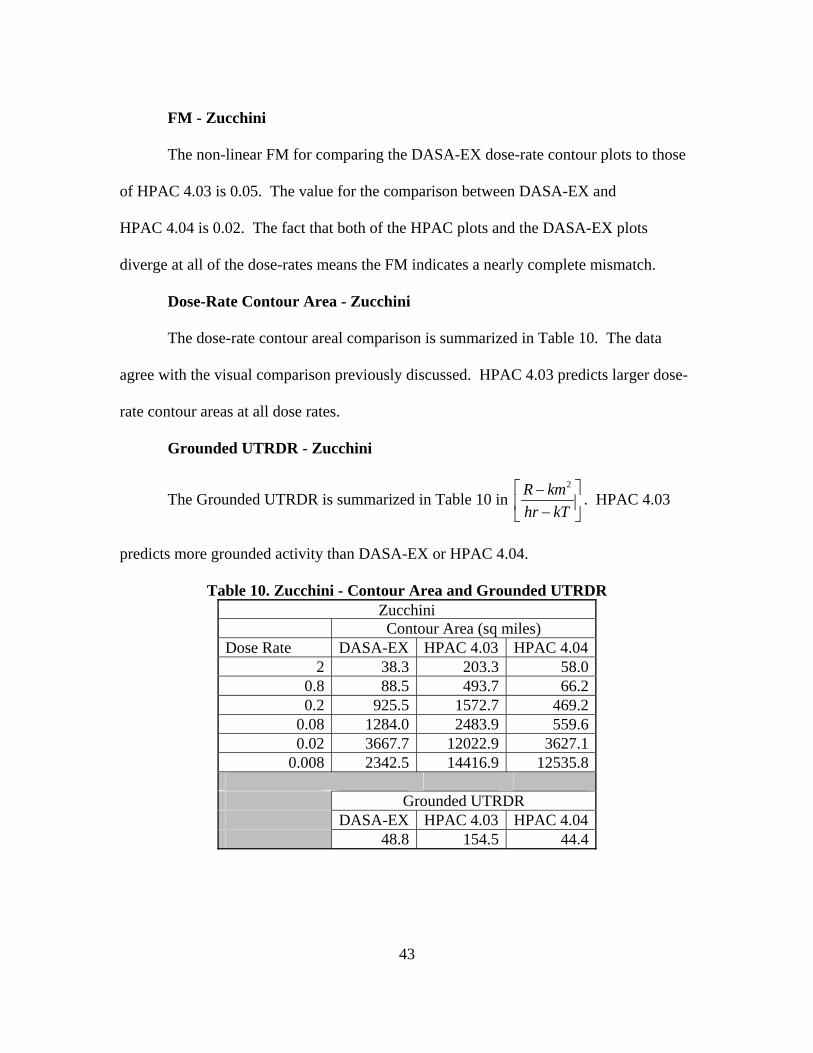
FM - Zucchini



HPAC 4.04 is 0.02. The fact that both of the HPAC plots and the DASA-EX plots

diverge at all of the dose-rates means the FM indicates a nearly complete mismatch.

Dose-Rate Contour Area - Zucchini

The dose-rate contour areal comparison is summarized in Table 10. The data

agree with the visual comparison previously discussed. HPAC 4.03 predicts larger dose-

rate contour areas at all dose rates.

Grounded UTRDR - Zucchini


hr kT⎡ ⎤−⎢ ⎥−⎣ ⎦

. HPAC 4.03

predicts more grounded activity than DASA-EX or HPAC 4.04.

Table 10. Zucchini - Contour Area and Grounded UTRDR Zucchini

Contour Area (sq miles) Dose Rate DASA-EX HPAC 4.03 HPAC 4.04

2 38.3 203.3 58.0 0.8 88.5 493.7 66.2 0.2 925.5 1572.7 469.2

0.08 1284.0 2483.9 559.6 0.02 3667.7 12022.9 3627.1


44

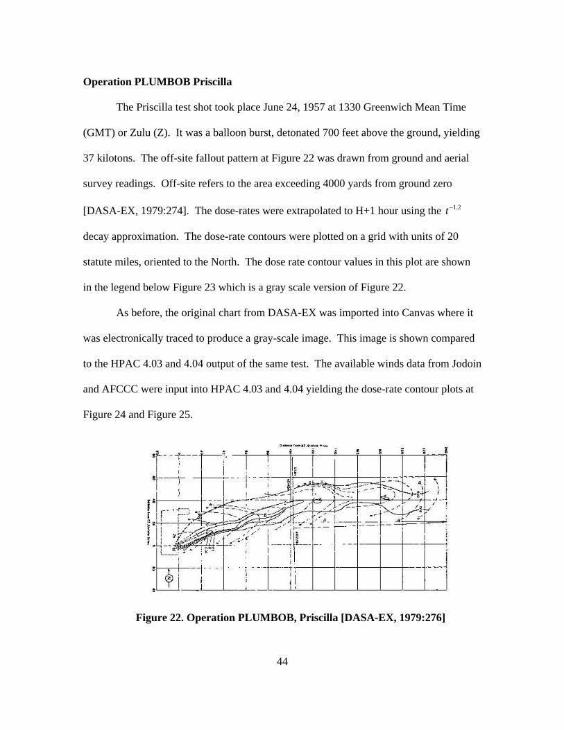
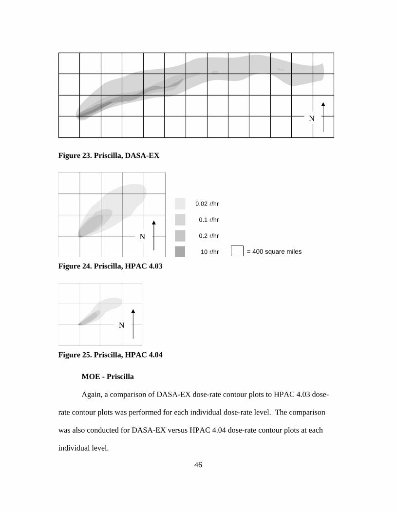
Operation PLUMBOB Priscilla

The Priscilla test shot took place June 24, 1957 at 1330 Greenwich Mean Time

(GMT) or Zulu (Z). It was a balloon burst, detonated 700 feet above the ground, yielding

37 kilotons. The off-site fallout pattern at Figure 22 was drawn from ground and aerial

survey readings. Off-site refers to the area exceeding 4000 yards from ground zero

[DASA-EX, 1979:274]. The dose-rates were extrapolated to H+1 hour using the 1.2t−

decay approximation. The dose-rate contours were plotted on a grid with units of 20

statute miles, oriented to the North. The dose rate contour values in this plot are shown

in the legend below Figure 23 which is a gray scale version of Figure 22.

As before, the original chart from DASA-EX was imported into Canvas where it

was electronically traced to produce a gray-scale image. This image is shown compared

to the HPAC 4.03 and 4.04 output of the same test. The available winds data from Jodoin

and AFCCC were input into HPAC 4.03 and 4.04 yielding the dose-rate contour plots at

Figure 24 and Figure 25.

Figure 22. Operation PLUMBOB, Priscilla [DASA-EX, 1979:276]

45

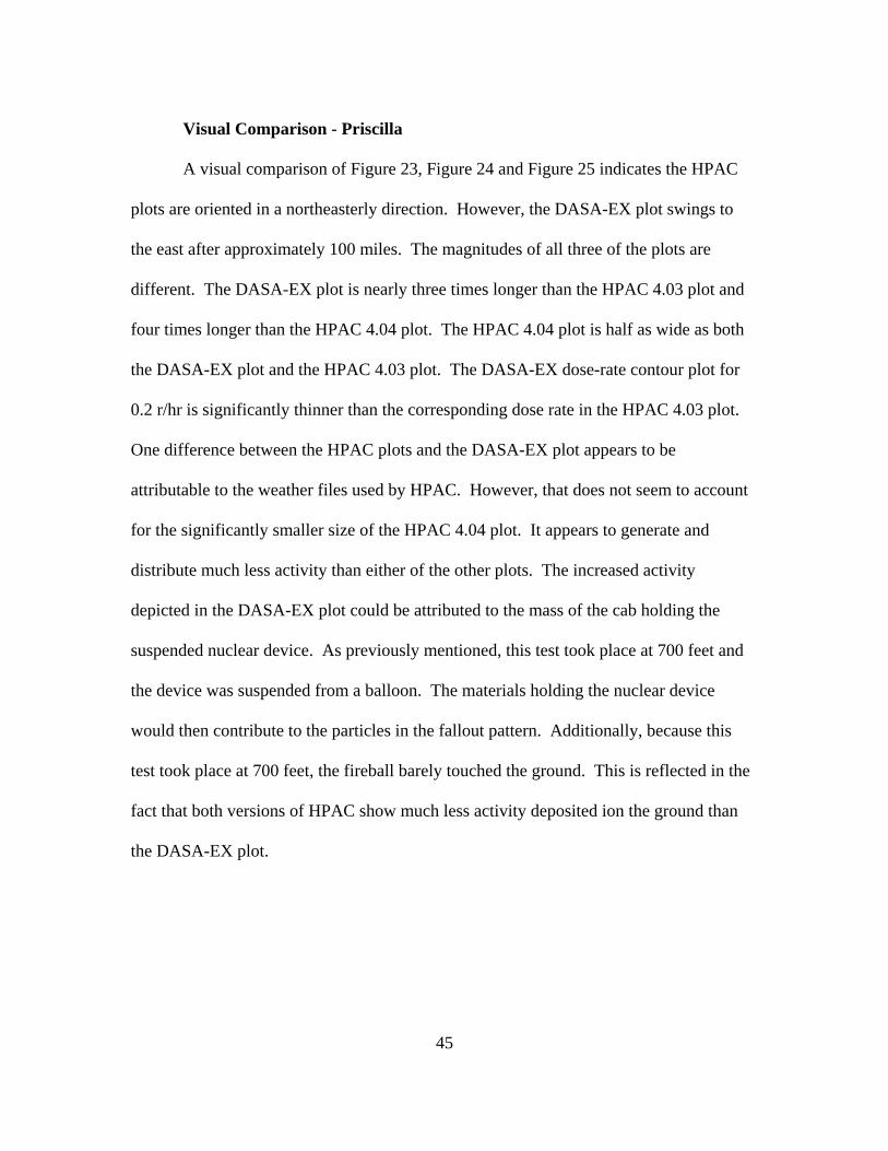
Visual Comparison - Priscilla

A visual comparison of Figure 23, Figure 24 and Figure 25 indicates the HPAC

plots are oriented in a northeasterly direction. However, the DASA-EX plot swings to

the east after approximately 100 miles. The magnitudes of all three of the plots are

different. The DASA-EX plot is nearly three times longer than the HPAC 4.03 plot and

four times longer than the HPAC 4.04 plot. The HPAC 4.04 plot is half as wide as both

the DASA-EX plot and the HPAC 4.03 plot. The DASA-EX dose-rate contour plot for

0.2 r/hr is significantly thinner than the corresponding dose rate in the HPAC 4.03 plot.

One difference between the HPAC plots and the DASA-EX plot appears to be

attributable to the weather files used by HPAC. However, that does not seem to account

for the significantly smaller size of the HPAC 4.04 plot. It appears to generate and

distribute much less activity than either of the other plots. The increased activity

depicted in the DASA-EX plot could be attributed to the mass of the cab holding the

suspended nuclear device. As previously mentioned, this test took place at 700 feet and

the device was suspended from a balloon. The materials holding the nuclear device

would then contribute to the particles in the fallout pattern. Additionally, because this

test took place at 700 feet, the fireball barely touched the ground. This is reflected in the

fact that both versions of HPAC show much less activity deposited ion the ground than

the DASA-EX plot.

46

Figure 23. Priscilla, DASA-EX

0.02 r/hr

0.1 r/hr

0.2 r/hr

10 r/hr Figure 24. Priscilla, HPAC 4.03

Figure 25. Priscilla, HPAC 4.04

MOE - Priscilla

Again, a comparison of DASA-EX dose-rate contour plots to HPAC 4.03 dose-

rate contour plots was performed for each individual dose-rate level. The comparison

was also conducted for DASA-EX versus HPAC 4.04 dose-rate contour plots at each

individual level.

= 400 square miles

N

N

N

47

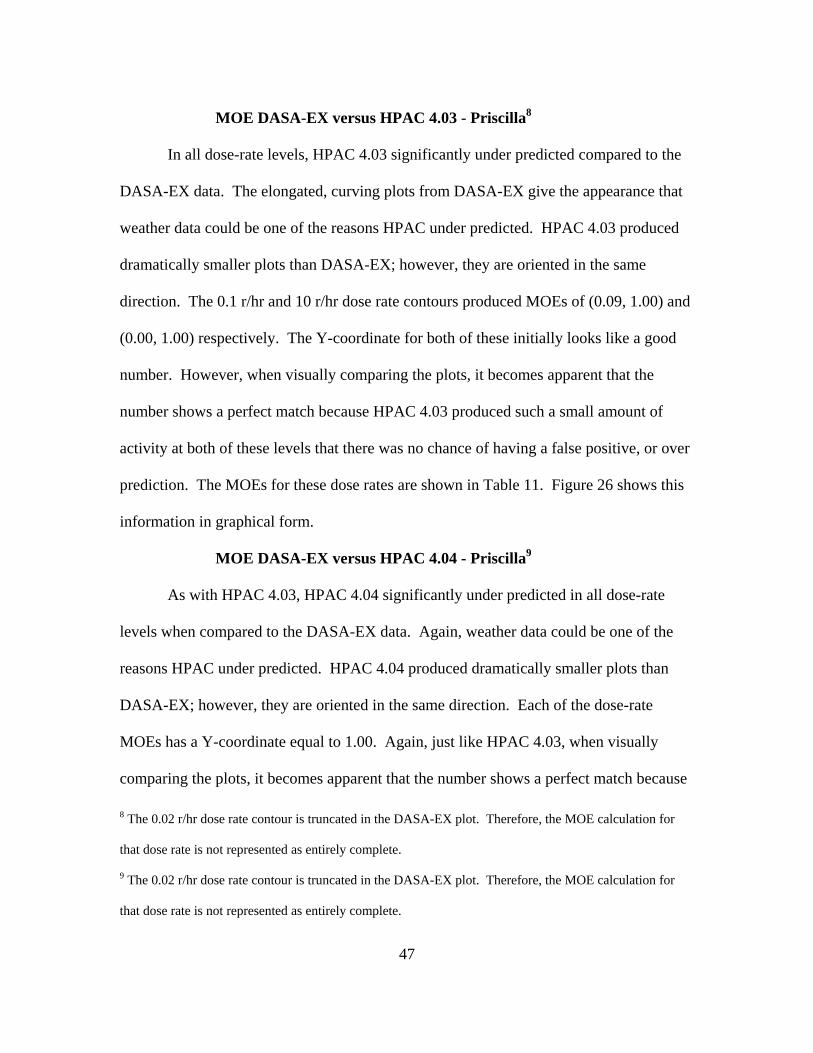
MOE DASA-EX versus HPAC 4.03 - Priscilla8

In all dose-rate levels, HPAC 4.03 significantly under predicted compared to the

DASA-EX data. The elongated, curving plots from DASA-EX give the appearance that

weather data could be one of the reasons HPAC under predicted. HPAC 4.03 produced

dramatically smaller plots than DASA-EX; however, they are oriented in the same

direction. The 0.1 r/hr and 10 r/hr dose rate contours produced MOEs of (0.09, 1.00) and

(0.00, 1.00) respectively. The Y-coordinate for both of these initially looks like a good

number. However, when visually comparing the plots, it becomes apparent that the

number shows a perfect match because HPAC 4.03 produced such a small amount of

activity at both of these levels that there was no chance of having a false positive, or over

prediction. The MOEs for these dose rates are shown in Table 11. Figure 26 shows this

information in graphical form.

MOE DASA-EX versus HPAC 4.04 - Priscilla9

As with HPAC 4.03, HPAC 4.04 significantly under predicted in all dose-rate

levels when compared to the DASA-EX data. Again, weather data could be one of the

reasons HPAC under predicted. HPAC 4.04 produced dramatically smaller plots than

DASA-EX; however, they are oriented in the same direction. Each of the dose-rate

MOEs has a Y-coordinate equal to 1.00. Again, just like HPAC 4.03, when visually

comparing the plots, it becomes apparent that the number shows a perfect match because





48

HPAC 4.04 produced such a small amount of activity at each of these levels that there

was no chance of having a false positive, or over prediction. The MOEs for these dose

rates are shown in Table 12. Figure 27 shows this information in graphical form.

Table 11. MOE Values - Priscilla, DASA-EX vs. HPAC 4.03

X Y Dose-Rate0.00 1.00 100.13 0.48 0.20.09 1.00 0.10.24 0.70 0.02

Priscilla

Priscilla MOEDASA-EX vs HPAC 4.03

0.0

0.2

0.4

0.6

0.8

1.0

0.0 0.2 0.4 0.6 0.8 1.0


Less

Ove

r-Pr

edic

tion

Dec

reas

ing

Fals

e Po

sitiv

e

0.02 r/hr0.1 r/hr0.2 r/hr10 r/hr

Figure 26. MOE - Priscilla, DASA-EX vs. HPAC 4.03

Table 12. MOE Values - Priscilla, DASA-EX vs. HPAC 4.04

X Y Dose-Rate0.01 1.00 100.08 1.00 0.20.02 1.00 0.10.09 1.00 0.02

Priscilla

Priscilla MOEDASA-EX vs HPAC 4.04

0.0

0.2

0.4

0.6

0.8

1.0

0.0 0.2 0.4 0.6 0.8 1.0


Less

Ove

r-Pr

edic

tion

Dec

reas

ing

Fals

e Po

sitiv

e

0.02 r/hr0.1 r/hr0.2 r/hr10 r/hr

Figure 27. MOE - Priscilla, DASA-EX vs. HPAC 4.04

49

50

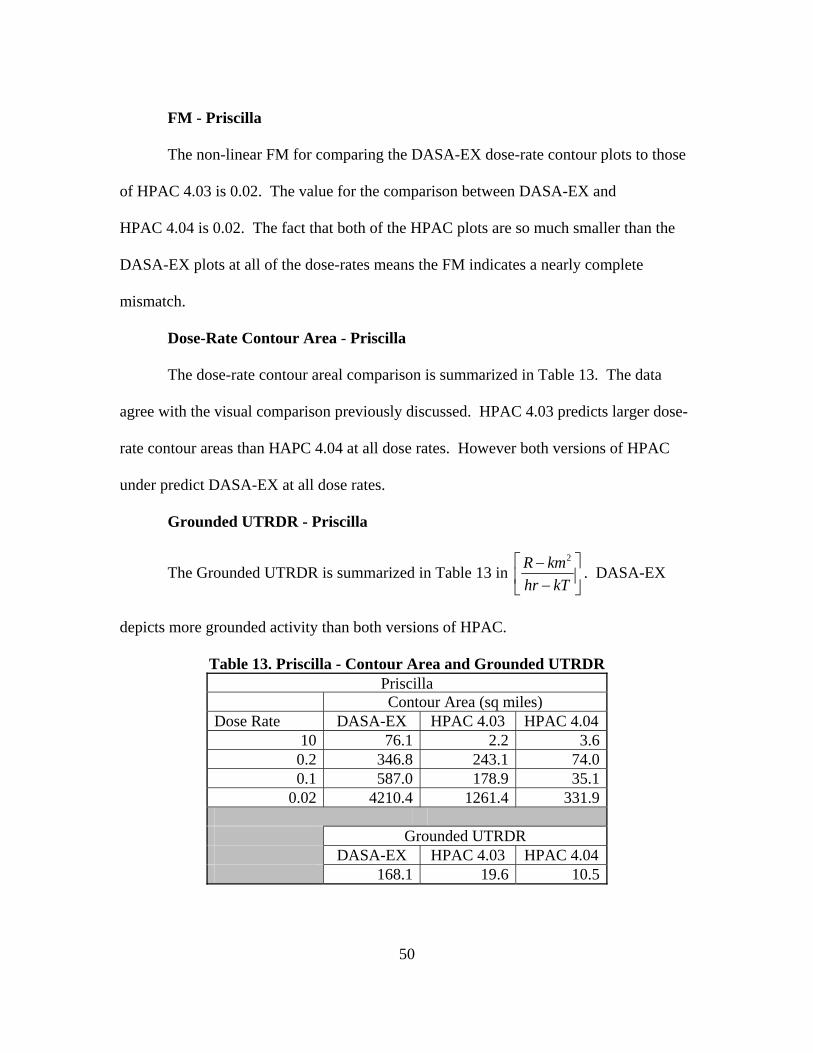
FM - Priscilla



HPAC 4.04 is 0.02. The fact that both of the HPAC plots are so much smaller than the

DASA-EX plots at all of the dose-rates means the FM indicates a nearly complete

mismatch.

Dose-Rate Contour Area - Priscilla



rate contour areas than HAPC 4.04 at all dose rates. However both versions of HPAC

under predict DASA-EX at all dose rates.

Grounded UTRDR - Priscilla


hr kT⎡ ⎤−⎢ ⎥−⎣ ⎦

. DASA-EX

depicts more grounded activity than both versions of HPAC.

Table 13. Priscilla - Contour Area and Grounded UTRDR Priscilla


10 76.1 2.2 3.6 0.2 346.8 243.1 74.0 0.1 587.0 178.9 35.1


51

Operation PLUMBOB Smoky

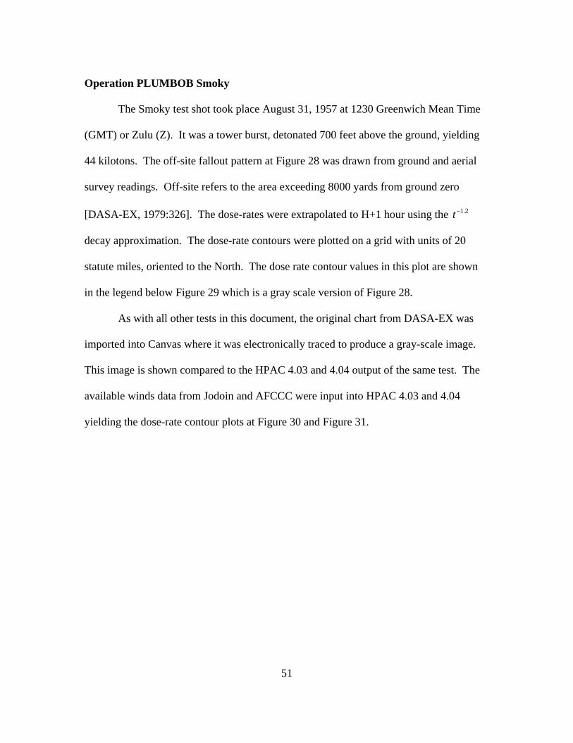
The Smoky test shot took place August 31, 1957 at 1230 Greenwich Mean Time


44 kilotons. The off-site fallout pattern at Figure 28 was drawn from ground and aerial

survey readings. Off-site refers to the area exceeding 8000 yards from ground zero

[DASA-EX, 1979:326]. The dose-rates were extrapolated to H+1 hour using the 1.2t−

decay approximation. The dose-rate contours were plotted on a grid with units of 20

statute miles, oriented to the North. The dose rate contour values in this plot are shown

in the legend below Figure 29 which is a gray scale version of Figure 28.

As with all other tests in this document, the original chart from DASA-EX was

imported into Canvas where it was electronically traced to produce a gray-scale image.

This image is shown compared to the HPAC 4.03 and 4.04 output of the same test. The

available winds data from Jodoin and AFCCC were input into HPAC 4.03 and 4.04

yielding the dose-rate contour plots at Figure 30 and Figure 31.

52

Figure 28. Operation PLUMBOB, Smoky [DASA-EX, 1979:328]

Visual Comparison - Smoky

A visual comparison of Figure 29, Figure 30 and Figure 31 indicates the three

plots are initially oriented in the east-southeast direction. However, the DASA-EX plot

swings to the northeast after approximately 100 miles. The magnitudes of all three of the

plots are different. The DASA-EX plot is nearly two times longer than the HPAC 4.03

plot and three times longer than the HPAC 4.04 plot. The HPAC 4.03 plot is nearly twice

as wide as both the DASA-EX plot and the HPAC 4.04 plot. As with previous tests, one

difference between the HPAC plots and the DASA-EX plot appears to be attributable to

the weather files used by HPAC. The long, dramatically curving shape of the DASA-EX

plot seems to indicate the weather file used by both versions of HPAC could benefit from

additional fidelity. However, that does not seem to completely account for the

53

significantly smaller size of both of the HPAC plots. The HPAC 4.04 plot appears to

generate and distribute much less activity than the HPAC 4.03 plot. The increased

activity depicted in the DASA-EX plot could be attributed to the mass of the cab holding

the suspended nuclear device. As previously mentioned, this test took place at 700 feet

and the device was suspended from a balloon. The materials holding the nuclear device

would then contribute to the particles in the fallout pattern. Additionally, because this

test took place at 700 feet, the fireball barely touched the ground. This is reflected in the

fact that both versions of HPAC show much less activity deposited ion the ground than

the DASA-EX plot.

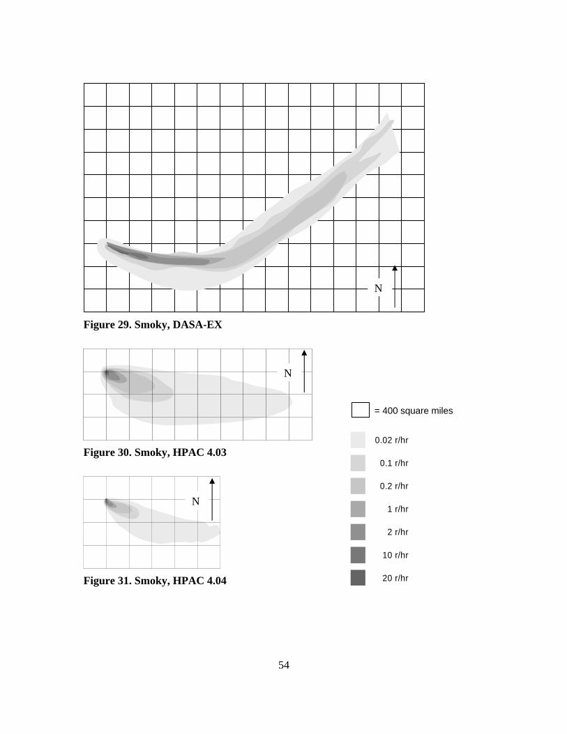
54

Figure 29. Smoky, DASA-EX

Figure 30. Smoky, HPAC 4.03

Figure 31. Smoky, HPAC 4.04

0.02 r/hr

0.1 r/hr

0.2 r/hr

1 r/hr

2 r/hr

10 r/hr

20 r/hr

= 400 square miles

N

N

N

55

MOE - Smoky




individual level.

MOE DASA-EX versus HPAC 4.03 - Smoky10

Similar to the Priscilla test, HPAC 4.03 significantly under predicted compared to

the DASA-EX data in all dose-rate levels. While the HPAC 4.03 plot is twice as wide as

the DASA-EX plot, it is only half as long. The 0.02 r/hr dose rate is the only contour plot

to generate a reasonable MOE (0.41, 0.57) in both the X and Y directions. This is due to

the sheer size of that dose-rate contour plot. It still is a significant under prediction

compared to the DASA-EX plot. The MOEs for all of the dose rates are shown in

Table 14. Figure 32 shows this information in graphical form.

MOE DASA-EX versus HPAC 4.04 - Smoky11

HPAC 4.04 significantly under predicted compared to the DASA-EX data in all

dose-rate levels. The dose-rate contour plot for 20 r/hr was so insignificant it produced a

MOE 0f (0.00, 0.00). The MOEs for all of the dose rates are shown in Table 15.

Figure 33 shows this information in graphical form.





Table 14. MOE Values - Smoky, DASA-EX vs. HPAC 4.03

X Y Dose-Rate0.00 0.00 200.01 0.05 100.07 0.47 20.12 0.51 10.13 0.51 0.20.15 0.54 0.10.41 0.57 0.02

Smoky

Smoky MOEDASA-EX vs HPAC 4.03

0.0

0.2

0.4

0.6

0.8

1.0

0.0 0.2 0.4 0.6 0.8 1.0


Less

Ove

r-Pr

edic

tion

Dec

reas

ing

Fals

e Po

sitiv

e

0.02 r/hr0.1 r/hr0.2 r/hr1 r/hr2 r/hr10 r/hr20 r/hr

Figure 32. MOE - Smoky, DASA-EX vs. HPAC 4.03

Table 15. MOE Values - Smoky, DASA-EX vs. HPAC 4.04

X Y Dose-Rate0.00 0.00 200.00 0.00 100.00 0.10 20.02 0.29 10.05 0.77 0.20.06 0.85 0.10.24 0.92 0.02

Smoky

Smoky MOEDASA-EX vs HPAC 4.04

0.0

0.2

0.4

0.6

0.8

1.0

0.0 0.2 0.4 0.6 0.8 1.0


Less

Ove

r-Pr

edic

tion

Dec

reas

ing

Fals

e Po

sitiv

e

0.02 r/hr0.1 r/hr0.2 r/hr1 r/hr2 r/hr10 r/hr20 r/hr

Figure 33. MOE - Smoky, DASA-EX vs. HPAC 4.04

56

57

FM - Smoky



HPAC 4.04 is 0.03. Again, the fact that both of the HPAC plots are so much smaller than

the DASA-EX plots at all of the dose-rates means the FM indicates a nearly complete

mismatch.

Dose-Rate Contour Area - Smoky



rate contour areas than HAPC 4.04 at all dose rates except the 20 r/hr. However both

versions of HPAC under predict DASA-EX at all dose rates except 2 r/hr and 0.02 r/hr.

Grounded UTRDR - Smoky


hr kT⎡ ⎤−⎢ ⎥−⎣ ⎦

. DASA-EX

depicts more grounded activity than both versions of HPAC.

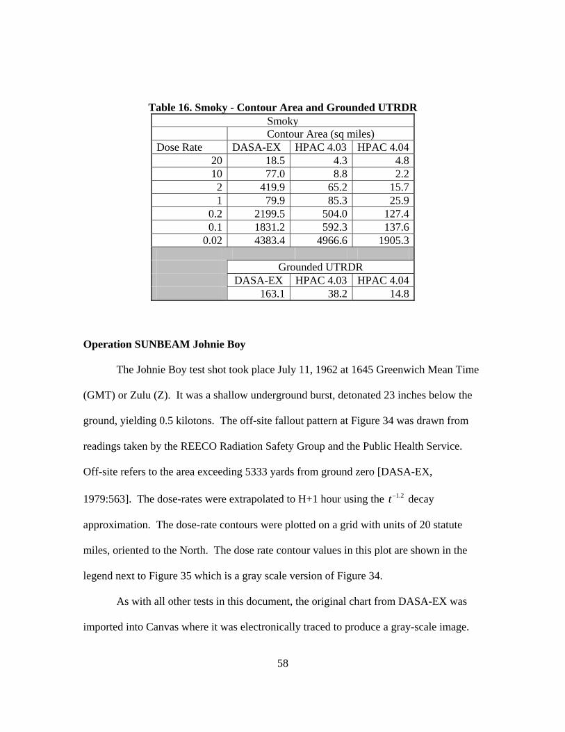
58

Table 16. Smoky - Contour Area and Grounded UTRDR Smoky


20 18.5 4.3 4.8 10 77.0 8.8 2.2 2 419.9 65.2 15.7 1 79.9 85.3 25.9

0.2 2199.5 504.0 127.4 0.1 1831.2 592.3 137.6


Operation SUNBEAM Johnie Boy

The Johnie Boy test shot took place July 11, 1962 at 1645 Greenwich Mean Time

(GMT) or Zulu (Z). It was a shallow underground burst, detonated 23 inches below the

ground, yielding 0.5 kilotons. The off-site fallout pattern at Figure 34 was drawn from

readings taken by the REECO Radiation Safety Group and the Public Health Service.

Off-site refers to the area exceeding 5333 yards from ground zero [DASA-EX,




legend next to Figure 35 which is a gray scale version of Figure 34.

As with all other tests in this document, the original chart from DASA-EX was

imported into Canvas where it was electronically traced to produce a gray-scale image.

59

This image is shown compared to the HPAC 4.03 and 4.04 output of the same test. The

available winds data from Jodoin and AFCCC were input into HPAC 4.03 and 4.04

yielding the dose-rate contour plots at Figure 36 and Figure 37.

Figure 34. Operation SUNBEAM, Johnie Boy [DASA-EX, 1979:565]

60

Visual Comparison - Johnie Boy

A visual comparison of Figure 35, Figure 36 and Figure 37 indicates the three

plots are oriented in a northeastern direction. The DASA-EX plot is half the size of both

of the HPAC plots. One reason for this is the level of uncertainty in producing the plot at

the time right after the test [DASA-EX, 1979:563] which limited the ability to plot the

dose-rate contours any further distance from ground zero.

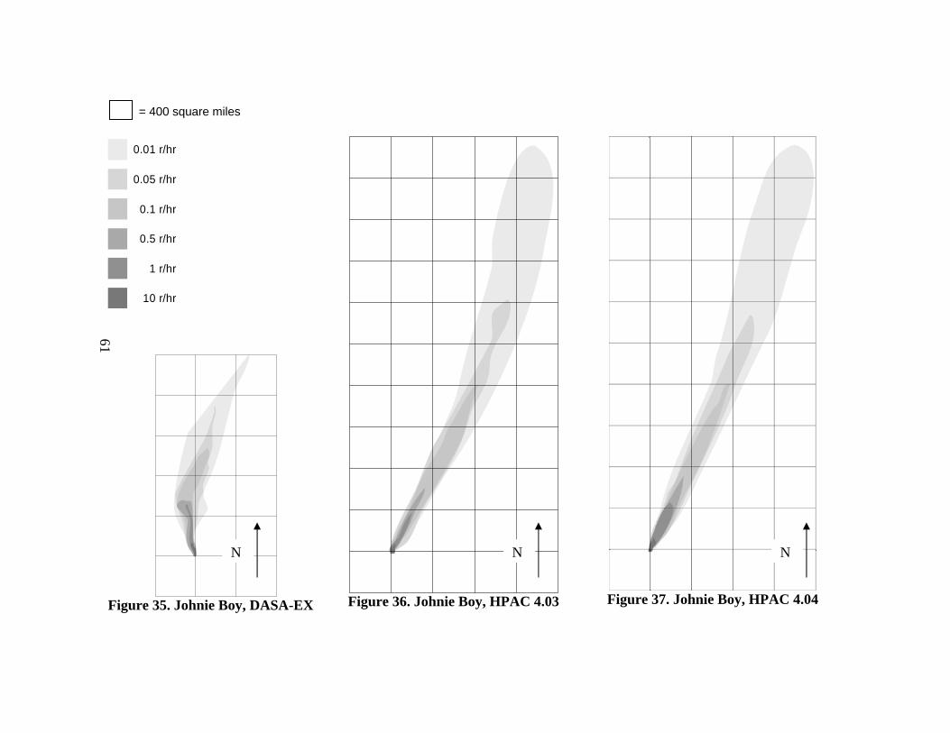
0.01 r/hr

0.05 r/hr

0.1 r/hr

0.5 r/hr

1 r/hr

10 r/hr

Figure 35. Johnie Boy, DASA-EX

Figure 36. Johnie Boy, HPAC 4.03

Figure 37. Johnie Boy, HPAC 4.04

= 400 square miles

NN N

61

62

MOE - Johnie Boy




individual level.

MOE DASA-EX versus HPAC 4.03 - Johnie Boy12

The DASA-EX plot is oriented to the north for approximately 40 miles before

shifting slightly to the north-northeast. Both of the HPAC plots are immediately oriented

to the northeast. All three of the plots are approximately 20 miles wide. Both of the

HPAC plots are very similar in magnitude and direction. Even though the DASA-EX

plot and the HPAC 4.03 plot are both oriented in similar directions, the slight difference

in initial directions yields MOEs that reflect no agreement, as indicated by Table 17.

Both the X and Y coordinates for all of the dose-rate levels are essentially zero.

Figure 38 shows this information in graphical form

MOE DASA-EX versus HPAC 4.04 - Johnie Boy13

This comparison is essentially the same as the previous case involving

HPAC 4.03. Even though the DASA-EX plot and the HPAC 4.04 plot are both oriented

in similar directions, the slight difference in initial directions yields MOEs that reflect no





63

agreement, as indicated by Table 18. Both the X and Y coordinates for all of the dose-

rate levels are essentially zero. Figure 39 shows this information in graphical form.

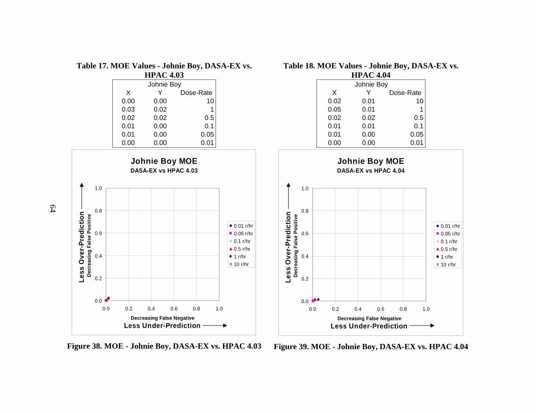
Table 17. MOE Values - Johnie Boy, DASA-EX vs. HPAC 4.03

X Y Dose-Rate0.00 0.00 100.03 0.02 10.02 0.02 0.50.01 0.00 0.10.01 0.00 0.050.00 0.00 0.01

Johnie Boy

Johnie Boy MOEDASA-EX vs HPAC 4.03

0.0

0.2

0.4

0.6

0.8

1.0

0.0 0.2 0.4 0.6 0.8 1.0


Less

Ove

r-Pr

edic

tion

Dec

reas

ing

Fals

e Po

sitiv

e

0.01 r/hr0.05 r/hr0.1 r/hr0.5 r/hr1 r/hr10 r/hr

Figure 38. MOE - Johnie Boy, DASA-EX vs. HPAC 4.03

Table 18. MOE Values - Johnie Boy, DASA-EX vs. HPAC 4.04

X Y Dose-Rate0.02 0.01 100.05 0.01 10.02 0.02 0.50.01 0.01 0.10.01 0.00 0.050.00 0.00 0.01

Johnie Boy

Johnie Boy MOEDASA-EX vs HPAC 4.04

0.0

0.2

0.4

0.6

0.8

1.0

0.0 0.2 0.4 0.6 0.8 1.0


Less

Ove

r-Pr

edic

tion

Dec

reas

ing

Fals

e Po

sitiv

e

0.01 r/hr0.05 r/hr0.1 r/hr0.5 r/hr1 r/hr10 r/hr

Figure 39. MOE - Johnie Boy, DASA-EX vs. HPAC 4.04

64

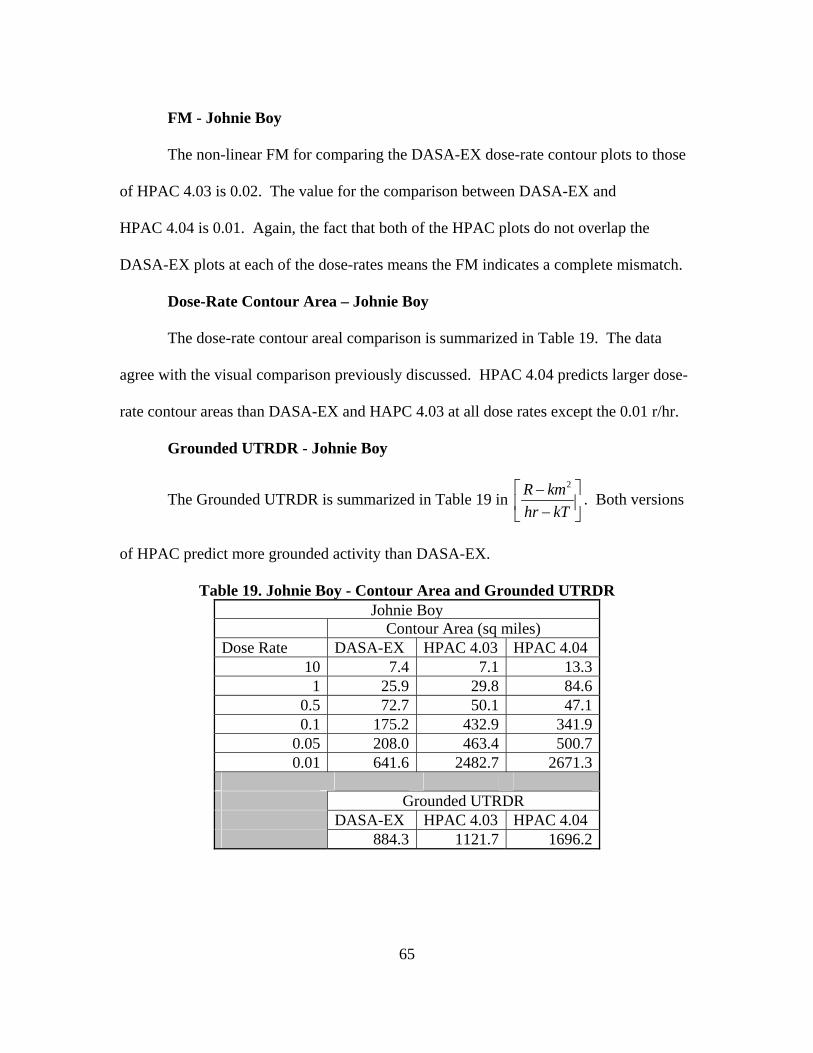
65

FM - Johnie Boy



HPAC 4.04 is 0.01. Again, the fact that both of the HPAC plots do not overlap the

DASA-EX plots at each of the dose-rates means the FM indicates a complete mismatch.

Dose-Rate Contour Area – Johnie Boy



rate contour areas than DASA-EX and HAPC 4.03 at all dose rates except the 0.01 r/hr.

Grounded UTRDR - Johnie Boy


hr kT⎡ ⎤−⎢ ⎥−⎣ ⎦

. Both versions

of HPAC predict more grounded activity than DASA-EX.

Table 19. Johnie Boy - Contour Area and Grounded UTRDR Johnie Boy


10 7.4 7.1 13.3 1 25.9 29.8 84.6

0.5 72.7 50.1 47.1 0.1 175.2 432.9 341.9

0.05 208.0 463.4 500.7 0.01 641.6 2482.7 2671.3

Grounded UTRDR DASA-EX HPAC 4.03 HPAC 4.04 884.3 1121.7 1696.2

66

IV. Summary and Conclusions

Chapter Overview

The purpose of this chapter is to present a summary of the results of the visual and

numerical comparisons of the different tests and provide recommendations for future

endeavors in this topic of research.

Results

The results of this research effort show definite trends regarding the dose-rate

contour plots of HPAC 4.03 and 4.04 when compared to the original data in DASA-EX.

Further, the use of visual comparisons and numerical analyses combined into one

document provides a capability previously unrealized. Although each of the techniques

used is not new, the combination provides future researchers a suite of tools to perform

multiple, independent analyses of the same data.

Visual Comparisons

In general, it can be seen that the HPAC 4.03 plots compare more favorably with

the DASA-EX plot than do the HPAC 4.04 plots. For the six tests evaluated, both HPAC

plots matched the general direction at the outset of each plot; although Ess, Priscilla and

Smoky had shifts in the DASA-EX plots that were not matched by HPAC. These shifts

appear to be caused by wind direction changes. Increased fidelity in the weather data

used by HPAC might alleviate the resulting mismatch farther into the contour plots.

DASA-EX showed unique spurs and eddies that were not apparent in either version of

HPAC. These could be traced to terrain subtleties not modeled in HPAC. They could

also be traced to data gathering techniques post-test.

67

It is interesting to note that Priscilla and Smoky have very thin, elongated contour

plots in DASA-EX while both versions of HPAC produce more rounded contours. The

increased activity depicted in both DASA-EX plots could be attributed to the mass of the

cab holding the suspended nuclear device. As previously mentioned, both tests took

place at 700 feet and the device was suspended from a balloon. The materials holding the

nuclear device would then contribute to the particles in the fallout pattern. Additionally,

because these tests took place at 700 feet, the fireball barely touched the ground. This is

reflected in the fact that both versions of HPAC show much less activity deposited ion

the ground than the DASA-EX plots. Another possible explanation is the fidelity of the

weather data used by HPAC as well as the way HPAC models transverse wind shear.

Finally, the visual comparisons clearly showed that HPAC 4.04 typically deposits less

activity than HPAC 4.03. This could be attributable to the use of the Heft distribution in

HPAC 4.04. It is possible that this distribution has such a large percentage of fallout

mass suspended as very fine particles that they do not deposit within the ranges covered

by DASA-EX or HPAC 4.04, if ever. Further information on this can be found with

Skaar [Skaar, 2005].

An additional consideration for the differences between the DASA-EX and HPAC

plots could be HPAC computed stabilized cloud height compared to those recorded in

DASA-EX. However, this was not evaluated in this research effort.

Numerical Comparisons

The numerical comparisons used in this research effort complemented the visual

comparisons with few unexpected results. The MOE used for each dose-rate contour

68

comparison between DASA-EX and each version of HPAC numerically reinforced what

was seen in the visual comparisons. For example, while HPAC might predict dose-rate

contours that appear to be the same magnitude and direction as those in DASA-EX, the

fact that the plots were not covering the exact same plot of ground meant they were

mismatches. The same held true for the FM method as well. In the case of the MOE

method, some dose rates were matched more closely than others; however, this does not

appear to be a function of increased modeling accuracy for that dose-rate.

The dose-rate areal comparisons corroborated the visual comparisons.

HPAC 4.03 typically predicted larger dose-rate contour areas than HPAC 4.04 in all

cases except Johnie Boy.

The Grounded UTRDR comparison revealed that HPAC 4.03 predicts more

activity than DASA-EX in four of the cases. The other two favored DASA-EX.

HPAC 4.04 predicted greater activity than DASA-EX in two of the cases (Ess and Johnie

Boy). It is noted that in all cases the Grounded UTRDR was considerably less than

theoretical values of the source normalization constant cited earlier. This is

unquestionably due to the step function integration that had to be used.

Recommendations for Future Research

In the future, research in this topic could include weather data with increased

fidelity. This would likely require the use of reanalysis data to show improved weather

trends over the areas in question. The effort could also benefit from high fidelity terrain

models to possibly capture some of the nuances shown in the DASA-EX plots. The

Grounded UTRDR could also be dramatically improved by converting the step-wise plots

69

in DASA-EX into continuous curves. Although the curves would not be actual data from

DASA-EX, they would allow for a reasoned approach to obtaining a more realistic

Grounded UTRDR value for each plot. Both versions of HPAC allow for near-

continuous data for the plots produced. The effort would be to perform the

metamorphosis of the DASA-EX data. A comparison of stabilized cloud heights between

HPAC and DASA-EX could also be performed.

70

Appendix A: Example of Process

Six tests were selected for this research effort; four were selected based on input

from the minutes of the Fallout Working Group and two were randomly selected by this

author. Each test was evaluated to ensure it was lower than the fallout free height of

burst. Following selection of a particular test, the dose-rate contour plot was extracted

from the DASA 1251-EX electronic PDF file and imported into Canvas software. The

image was traced over each dose-rate contour line using Canvas software. This was done

in successive steps until the entire set of dose-rate contour lines was traced. Each dose-

rate contour line was then filled in using successively darker gray-scale colors for each

increase in dose rate. A grid was then inserted over the document based on the scale

contained in DASA-EX. The scale is 20 miles by 20 miles for each grid square. Dots

were then marked on key intersections of the grid to provide data interpretation at later

steps. The image was then saved as a gray-scale TIF file on a scale designed to produce

three pixels for statute mile within the picture; therefore, each square mile is represented

by nine pixels. For example, if the original DASA-EX diagram was 120 miles wide by

240 miles long, the resulting TIF file was saved to a resolution of 361 pixels wide by 721

pixels long. This represents three pixels per linear mile plus one pixel for the edge of the

grid.

The TIF file was imported in to MATLAB as a gray-scale image. MATLAB

imports this image in a pixel-by-pixel fashion and assigns gray-scale values ranging from

255 (white space) to 0 (black space) to each pixel. The black dots previously inserted

were located as zeros within the MATLAB image array. From there the exact pixel

representing ground zero was determined and the contour values for the image were then

71

interpreted from there. This yields a gridded image from DASA-EX that can be

compared to the HPAC output.

The HPAC output was obtained by entering the details of the test event into each

version of HPAC. Dose rate contour plots were obtained by selecting the custom output

option and entering dose rates of interest. The dose rates of interest were obtained by

observing the HPAC run time for each event and then using the 1.2t− decay rate

approximation to determine the dose rate at H+1 hour. This method was used because

HPAC does not plot H+1 hour dose rates as a function of final dose rate. However,

DASA-EX is plotted in H=1 hour dose rates. The custom plot was then saved as a JPEG

file and imported into Canvas. From there, the picture was processed like the DASA-EX

pictures were processed as mentioned earlier. The document was set to scale using the

option available in Canvas and the ruler embedded in the HPAC plot picture. A 20 mile

by 20 mile grid was then inserted on top of the picture to facilitate visual comparisons

between both versions of HPAC as well as the DASA-EX plots. The image was saved in

gray-scale format and imported in to MATLAB. This yields a gridded image that can be

compared point to point with the Canvas image using the gray scale values which now

represent dose-rates.

72

Appendix B: Weather Profiles

HPAC uses several types of weather data. They are focused in two main areas:

real-time/forecasts and past. Because this research effort involved events that already

occurred, the option involving real-time and forecast data are not addressed. For events

that have already occurred, HPAC offers the option of using historical data or specific

data for specific events. The historical data option makes use of upper air climatology

data for two days of each month from 1990. According to the literature, this year was

chosen arbitrarily. The two days are the 15th and 16th of each month. HPAC chooses

which day to use based on the start date of the particular project [DTRA, 2003:A-2]. In

this case, actual data were available; therefore, the historical option was not used.

This research effort involved six nuclear tests that took place between 1952 and

1962. Weather data were available for these tests; however, it was not readily available.

Some weather observation data were available in Jodoin for each of the events. These

data were derived from DASA-EX and other unclassified sources. The data were in the

form of a profile observation. However, this single observation did not add much fidelity

to either of the HPAC models. The lack of weather updates caused the models to predict

fallout contour plots that were oriented in one direction following the bomb detonation.

To improve upon this, additional weather observations were obtained through the Air

Force Combat Climatology Center (AFCCC). This author requested weather data for

each of the tests for a period beginning at test time through seven days after the test.

These data were received from AFCCC as Rawinsonde Observations (RAOBS) in a

format that was not immediately useable by either version of HPAC. However, after a

few modifications to the files, they were in the correct format. These modifications

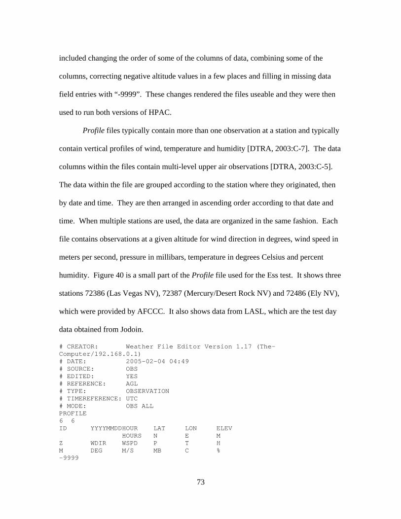
73

included changing the order of some of the columns of data, combining some of the

columns, correcting negative altitude values in a few places and filling in missing data

field entries with “-9999”. These changes rendered the files useable and they were then

used to run both versions of HPAC.

Profile files typically contain more than one observation at a station and typically

contain vertical profiles of wind, temperature and humidity [DTRA, 2003:C-7]. The data

columns within the files contain multi-level upper air observations [DTRA, 2003:C-5].

The data within the file are grouped according to the station where they originated, then

by date and time. They are then arranged in ascending order according to that date and

time. When multiple stations are used, the data are organized in the same fashion. Each

file contains observations at a given altitude for wind direction in degrees, wind speed in

meters per second, pressure in millibars, temperature in degrees Celsius and percent

humidity. Figure 40 is a small part of the Profile file used for the Ess test. It shows three

stations 72386 (Las Vegas NV), 72387 (Mercury/Desert Rock NV) and 72486 (Ely NV),

which were provided by AFCCC. It also shows data from LASL, which are the test day

data obtained from Jodoin.

# CREATOR: Weather File Editor Version 1.17 (The-Computer/192.168.0.1) # DATE: 2005-02-04 04:49 # SOURCE: OBS # EDITED: YES # REFERENCE: AGL # TYPE: OBSERVATION # TIMEREFERENCE: UTC # MODE: OBS ALL PROFILE 6 6 ID YYYYMMDDHOUR LAT LON ELEV HOURS N E M Z WDIR WSPD P T H M DEG M/S MB C % -9999

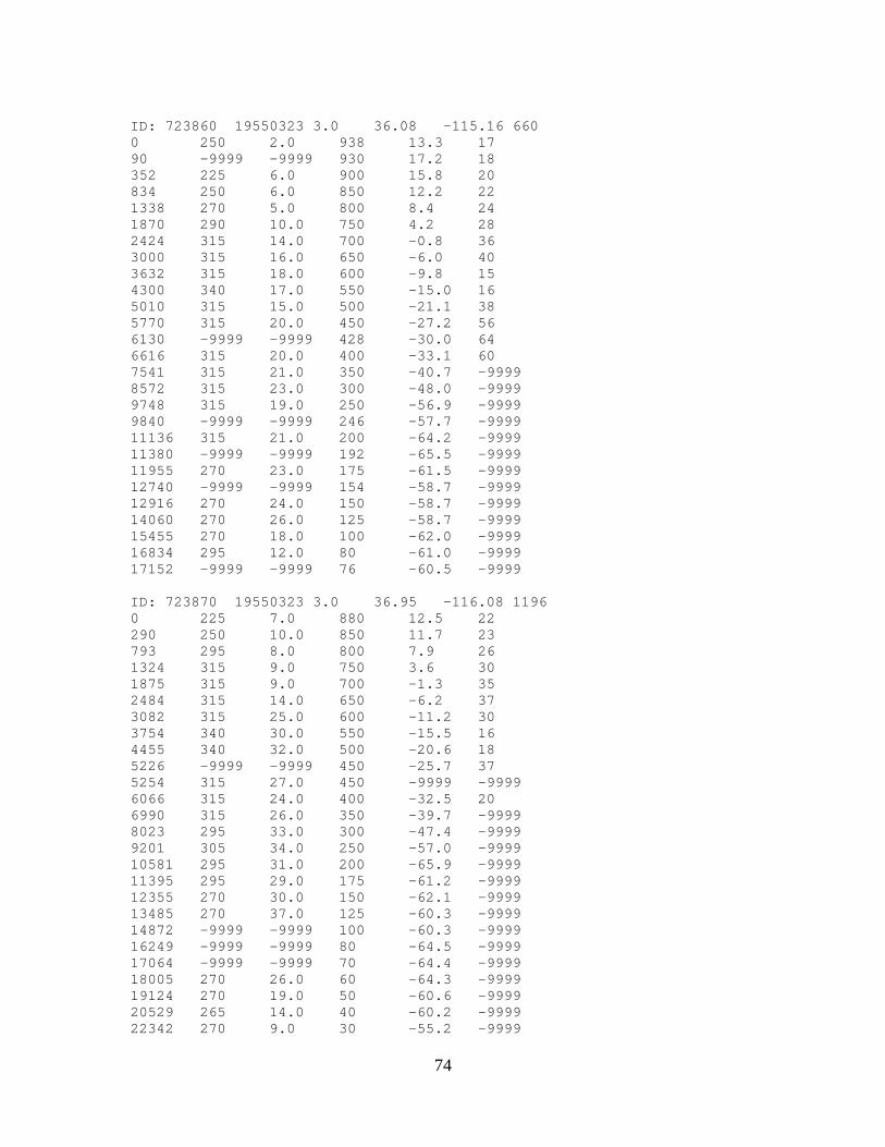
74

ID: 723860 19550323 3.0 36.08 -115.16 660 0 250 2.0 938 13.3 17 90 -9999 -9999 930 17.2 18 352 225 6.0 900 15.8 20 834 250 6.0 850 12.2 22 1338 270 5.0 800 8.4 24 1870 290 10.0 750 4.2 28 2424 315 14.0 700 -0.8 36 3000 315 16.0 650 -6.0 40 3632 315 18.0 600 -9.8 15 4300 340 17.0 550 -15.0 16 5010 315 15.0 500 -21.1 38 5770 315 20.0 450 -27.2 56 6130 -9999 -9999 428 -30.0 64 6616 315 20.0 400 -33.1 60 7541 315 21.0 350 -40.7 -9999 8572 315 23.0 300 -48.0 -9999 9748 315 19.0 250 -56.9 -9999 9840 -9999 -9999 246 -57.7 -9999 11136 315 21.0 200 -64.2 -9999 11380 -9999 -9999 192 -65.5 -9999 11955 270 23.0 175 -61.5 -9999 12740 -9999 -9999 154 -58.7 -9999 12916 270 24.0 150 -58.7 -9999 14060 270 26.0 125 -58.7 -9999 15455 270 18.0 100 -62.0 -9999 16834 295 12.0 80 -61.0 -9999 17152 -9999 -9999 76 -60.5 -9999 ID: 723870 19550323 3.0 36.95 -116.08 1196 0 225 7.0 880 12.5 22 290 250 10.0 850 11.7 23 793 295 8.0 800 7.9 26 1324 315 9.0 750 3.6 30 1875 315 9.0 700 -1.3 35 2484 315 14.0 650 -6.2 37 3082 315 25.0 600 -11.2 30 3754 340 30.0 550 -15.5 16 4455 340 32.0 500 -20.6 18 5226 -9999 -9999 450 -25.7 37 5254 315 27.0 450 -9999 -9999 6066 315 24.0 400 -32.5 20 6990 315 26.0 350 -39.7 -9999 8023 295 33.0 300 -47.4 -9999 9201 305 34.0 250 -57.0 -9999 10581 295 31.0 200 -65.9 -9999 11395 295 29.0 175 -61.2 -9999 12355 270 30.0 150 -62.1 -9999 13485 270 37.0 125 -60.3 -9999 14872 -9999 -9999 100 -60.3 -9999 16249 -9999 -9999 80 -64.5 -9999 17064 -9999 -9999 70 -64.4 -9999 18005 270 26.0 60 -64.3 -9999 19124 270 19.0 50 -60.6 -9999 20529 265 14.0 40 -60.2 -9999 22342 270 9.0 30 -55.2 -9999

75

23513 -9999 -9999 25 -55.7 -9999 24942 270 9.0 20 -56.3 -9999 ID: 724860 19550323 3.0 39.28 -114.85 1913 0 155 3.0 807 1.0 52 66 205 4.0 800 3.0 47 167 -9999 -9999 792 5.5 35 587 295 9.0 750 2.0 38 1144 295 12.0 700 -2.4 43 1727 295 15.0 650 -7.5 51 2344 295 17.0 600 -13.0 63 3007 315 22.0 550 -18.8 74 3327 -9999 -9999 527 -20.9 71 3705 295 23.0 500 -21.6 47 4487 295 35.0 450 -26.2 49 5320 -9999 -9999 400 -31.2 35 6248 -9999 -9999 350 -39.5 22 7280 -9999 -9999 300 -48.2 -9999 8027 -9999 -9999 268 -54.2 -9999 8452 -9999 -9999 250 -56.6 -9999 9841 -9999 -9999 200 -63.4 -9999 10007 -9999 -9999 195 -64.2 -9999 10655 -9999 -9999 175 -65.0 -9999 11605 -9999 -9999 150 -59.3 -9999 12743 -9999 -9999 125 -59.2 -9999 14146 -9999 -9999 100 -55.9 -9999 14387 -9999 -9999 96 -55.0 -9999 15548 -9999 -9999 80 -61.2 -9999 16387 -9999 -9999 70 -60.6 -9999 17358 -9999 -9999 60 -60.0 -9999 18506 -9999 -9999 50 -57.9 -9999 19904 -9999 -9999 40 -58.0 -9999 21716 -9999 -9999 30 -56.2 -9999 22155 -9999 -9999 28 -55.8 -9999 ID: 723870 19550323 9.0 36.95 -116.08 1196 0 45 0.0 882 12.0 39 305 270 3.0 850 9.4 29 803 295 5.0 800 5.8 27 1324 315 7.0 750 2.1 25 1881 295 13.0 700 -1.3 14 2464 295 16.0 650 -5.3 15 3090 315 18.0 600 -10.2 37 3754 315 21.0 550 -14.5 41 4472 315 20.0 500 -18.3 17 5224 315 18.0 450 -25.1 32 6066 -9999 -9999 400 -32.8 20 6094 315 23.0 400 -9999 -9999 6992 -9999 -9999 350 -40.0 -9999 7019 315 24.0 350 -9999 -9999 8025 -9999 -9999 300 -48.5 -9999 8051 315 23.0 300 -9999 -9999 9222 315 31.0 250 -58.0 -9999 10595 295 28.0 200 -66.4 -9999 11397 295 31.0 175 -68.2 -9999 12354 295 23.0 150 -58.0 -9999

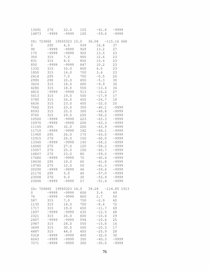
76

13491 270 22.0 125 -61.8 -9999 14873 -9999 -9999 100 -59.6 -9999 ID: 723860 19550323 15.0 36.08 -115.16 660 0 295 4.0 939 16.8 37 90 -9999 -9999 929 13.2 27 170 -9999 -9999 920 13.5 23 355 315 7.0 900 12.6 23 831 315 8.0 850 10.4 23 850 -9999 -9999 847 10.2 23 1332 315 10.0 800 6.5 23 1850 315 14.0 750 3.4 23 2414 295 7.0 700 -0.5 26 2990 290 10.0 650 -5.3 30 3624 315 18.0 600 -9.9 36 4280 315 18.0 550 -13.4 34 4810 -9999 -9999 513 -16.2 27 5013 315 19.0 500 -17.9 17 5780 315 24.0 450 -24.7 18 6636 315 23.0 400 -32.0 20 7562 315 23.0 350 -40.1 -9999 8593 315 25.0 300 -48.8 -9999 9765 315 29.0 250 -58.2 -9999 10500 -9999 -9999 223 -63.3 -9999 10970 -9999 -9999 206 -63.3 -9999 11145 295 32.0 200 -63.9 -9999 11710 -9999 -9999 182 -66.1 -9999 11960 295 26.0 175 -63.0 -9999 12915 270 26.0 150 -60.0 -9999 13340 -9999 -9999 140 -58.2 -9999 14060 270 27.0 125 -58.2 -9999 15457 270 25.0 100 -60.7 -9999 16847 270 23.0 80 -59.2 -9999 17680 -9999 -9999 70 -60.4 -9999 18636 295 19.0 60 -61.8 -9999 19765 270 12.0 50 -61.5 -9999 20290 -9999 -9999 46 -59.6 -9999 21176 295 5.0 40 -57.0 -9999 23008 270 9.0 30 -53.9 -9999 23690 -9999 -9999 27 -51.4 -9999 ID: 724860 19550323 16.0 39.28 -114.85 1913 0 -9999 -9999 808 3.4 49 76 -9999 -9999 800 2.7 50 587 315 7.0 750 -2.9 60 1135 315 14.0 700 -8.4 72 1717 315 19.0 650 -11.7 69 1897 -9999 -9999 635 -12.5 68 2321 315 24.0 600 -10.6 29 2407 -9999 -9999 594 -10.6 25 2987 315 28.0 550 -15.8 16 3699 315 30.0 500 -20.3 17 4487 315 44.0 450 -25.9 28 5318 -9999 -9999 400 -32.0 30 6243 -9999 -9999 350 -40.3 -9999 7271 -9999 -9999 300 -50.0 -9999

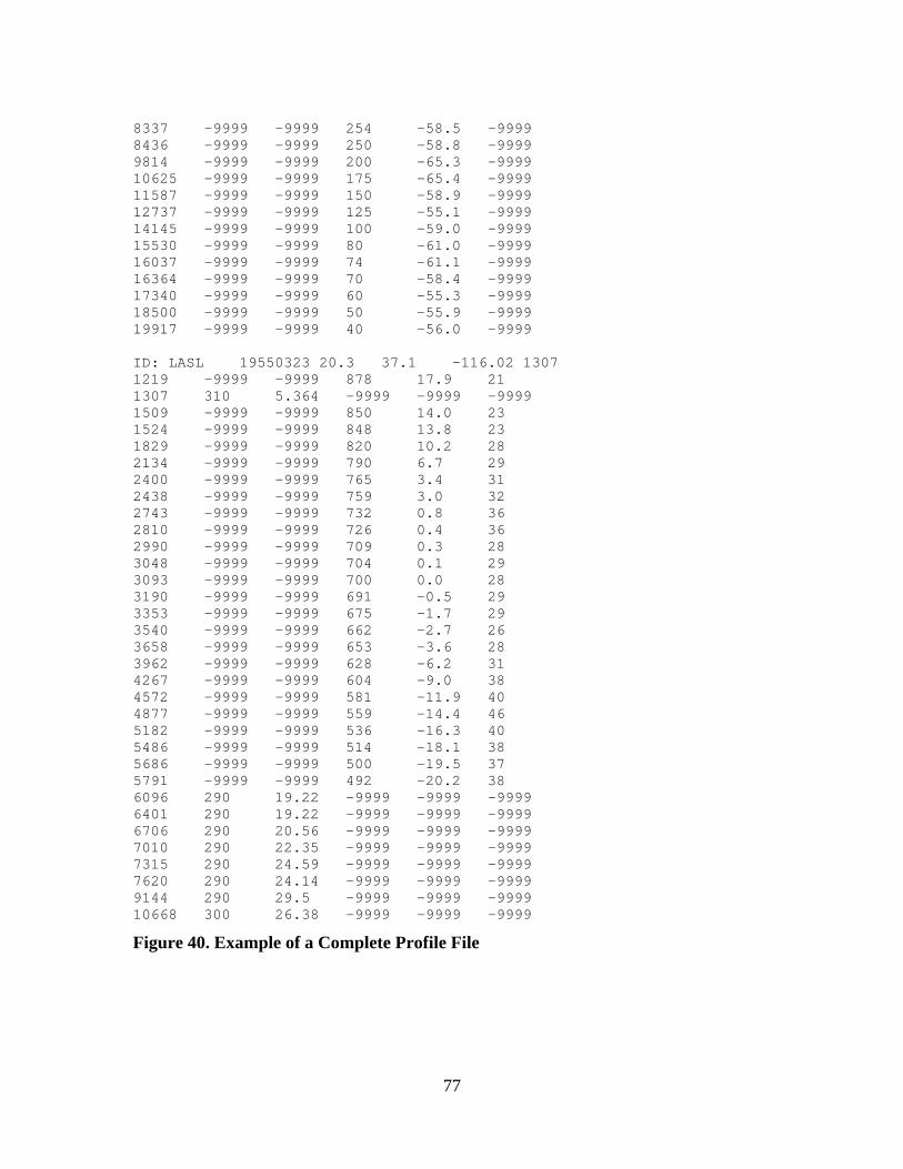
77

8337 -9999 -9999 254 -58.5 -9999 8436 -9999 -9999 250 -58.8 -9999 9814 -9999 -9999 200 -65.3 -9999 10625 -9999 -9999 175 -65.4 -9999 11587 -9999 -9999 150 -58.9 -9999 12737 -9999 -9999 125 -55.1 -9999 14145 -9999 -9999 100 -59.0 -9999 15530 -9999 -9999 80 -61.0 -9999 16037 -9999 -9999 74 -61.1 -9999 16364 -9999 -9999 70 -58.4 -9999 17340 -9999 -9999 60 -55.3 -9999 18500 -9999 -9999 50 -55.9 -9999 19917 -9999 -9999 40 -56.0 -9999 ID: LASL 19550323 20.3 37.1 -116.02 1307 1219 -9999 -9999 878 17.9 21 1307 310 5.364 -9999 -9999 -9999 1509 -9999 -9999 850 14.0 23 1524 -9999 -9999 848 13.8 23 1829 -9999 -9999 820 10.2 28 2134 -9999 -9999 790 6.7 29 2400 -9999 -9999 765 3.4 31 2438 -9999 -9999 759 3.0 32 2743 -9999 -9999 732 0.8 36 2810 -9999 -9999 726 0.4 36 2990 -9999 -9999 709 0.3 28 3048 -9999 -9999 704 0.1 29 3093 -9999 -9999 700 0.0 28 3190 -9999 -9999 691 -0.5 29 3353 -9999 -9999 675 -1.7 29 3540 -9999 -9999 662 -2.7 26 3658 -9999 -9999 653 -3.6 28 3962 -9999 -9999 628 -6.2 31 4267 -9999 -9999 604 -9.0 38 4572 -9999 -9999 581 -11.9 40 4877 -9999 -9999 559 -14.4 46 5182 -9999 -9999 536 -16.3 40 5486 -9999 -9999 514 -18.1 38 5686 -9999 -9999 500 -19.5 37 5791 -9999 -9999 492 -20.2 38 6096 290 19.22 -9999 -9999 -9999 6401 290 19.22 -9999 -9999 -9999 6706 290 20.56 -9999 -9999 -9999 7010 290 22.35 -9999 -9999 -9999 7315 290 24.59 -9999 -9999 -9999 7620 290 24.14 -9999 -9999 -9999 9144 290 29.5 -9999 -9999 -9999 10668 300 26.38 -9999 -9999 -9999

Figure 40. Example of a Complete Profile File

78

Bibliography

Bridgman, Charles J. “Introduction to the Physics of Nuclear Weapons Effects,” Defense Threat Reduction Agency, 8725 John J. Kingman Road, Fort Belvoir VA 22060-6201, 2001.

Canvas. Version 9.0.4, CD, Computer Software. ACD Systems Inc., 2004.

DASA 1251-1-EX. “Compilation of Local Fallout Data from Test Detonations 1945-1962 Extracted from DASA 1251. Volume I - Continental U.S. Tests,” Defense Nuclear Agency, Washington D.C., 1979.

Defense Threat Reduction Agency (DTRA). Fallout Working Group Minutes, Alexandria VA, July 2003.

DTRA. Hazard Prediction and Assessment Capability (HPAC), User Guide, Version 4.03. Alexandria VA, 2003.

DTRA. Hazard Prediction and Assessment Capability (HPAC), User Guide, Version 4.04. Alexandria VA, 2004.

DTRA. HPAC, Primer of Nuclear, Biological, and Chemical Weapons and Effects, Version 4.0. Alexandria VA, 2001.

Glasstone, Samuel and Dolan, Philip J. “The Effects of Nuclear Weapons,” Third Edition, Department of Defense and Department of Energy, 1977.

Heft, Robert E. “The Characterization of Radioactive Particles from Nuclear Weapons Tests,” Radionuclides in the Environment. Washington DC: American Chemical Society, 1970.

Jodoin, Vincent J. “Nuclear Cloud Rise and Growth,” AFIT Dissertation AFIT/DS/ENP/94J-2, June 1994.

McGahan, Joseph T. “Results of Fallout Model Validation,” SAIC, Alexandria VA, 2004.

McGahan, Joseph T. Personal Correspondence with Skaar, E.T., SAIC, Alexandria VA, October 13, 2004.

Rowland, R. H. and Thompson, J. H. “A Method for Comparing Fallout Patterns,” Defense Nuclear Agency, Washington D.C., 1972.

79

Skaar, E.T. “A Comparison Of The Heft Subsurface and DELFIC Particle Size Distributions And Effects in HPAC,” 2005, unpublished.

Sykes, R. I., et al. PC-SCIPUFF Version 1.2PD, Technical Documentation, Titan Corporation, Princeton NJ, 1998.

Warner, S. Institute for Defense Analysis, Alexandria VA. Telephone Interview. 2 February 2005.

Warner, S., et al. “User-Oriented Measures of Effectiveness for the Evaluation of Transport and Dispersion Models,” Institute for Defense Analyses, Alexandria VA, 2001.

Warner, S., et al. “User-Oriented Measures of Effectiveness for the Evaluation of Transport and Dispersion Models,” Institute for Defense Analyses, Alexandria VA, 2002.

REPORT DOCUMENTATION PAGE Form Approved OMB No. 074-0188

The public reporting burden for this collection of information is estimated to average 1 hour per response, including the time for reviewing instructions, searching existing data sources, gathering and maintaining the data needed, and completing and reviewing the collection of information. Send comments regarding this burden estimate or any other aspect of the collection of information, including suggestions for reducing this burden to Department of Defense, Washington Headquarters Services, Directorate for Information Operations and Reports (0704-0188), 1215 Jefferson Davis Highway, Suite 1204, Arlington, VA 22202-4302. Respondents should be aware that notwithstanding any other provision of law, no person shall be subject to a penalty for failing to comply with a collection of information if it does not display a currently valid OMB control number. PLEASE DO NOT RETURN YOUR FORM TO THE ABOVE ADDRESS. 1. REPORT DATE (DD-MM-YYYY)

21 Mar 05 2. REPORT TYPE

Master’s Thesis 3. DATES COVERED (From – To)

March 2002 – March 2003 5a. CONTRACT NUMBER

5b. GRANT NUMBER

4. TITLE AND SUBTITLE A Comparison Of Hazard Prediction And Assessment Capability (HPAC) Software Dose-Rate Contour Plots To A Sample Of Local Fallout Data From Test Detonations In The Continental United States, 1945 - 1962

5c. PROGRAM ELEMENT NUMBER

5d. PROJECT NUMBER 5e. TASK NUMBER

6. AUTHOR(S) Chancellor, Richard W., Major, USAF

5f. WORK UNIT NUMBER

7. PERFORMING ORGANIZATION NAMES(S) AND ADDRESS(S) Air Force Institute of Technology Graduate School of Engineering and Management (AFIT/EN) 2950 Hobson Way WPAFB OH 45433-7765

8. PERFORMING ORGANIZATION REPORT NUMBER AFIT/GNE/ENP/05-02

10. SPONSOR/MONITOR’S ACRONYM(S)

9. SPONSORING/MONITORING AGENCY NAME(S) AND ADDRESS(ES) Defense Threat Reduction Agency ATTN: TDOC 8725 John J. Kingman Rd, MS 6201 MAJ Robert Sobeski Fort Belvoir VA 22060-6201 DSN 221-7178

11. SPONSOR/MONITOR’S REPORT NUMBER(S)

12. DISTRIBUTION/AVAILABILITY STATEMENT APPROVED FOR PUBLIC RELEASE; DISTRIBUTION IS UNLIMITED.

13. SUPPLEMENTARY NOTES

14. ABSTRACT A comparison of Hazard Prediction and Assessment Capability (HPAC) software dose-rate contour plots to a sample of local nuclear fallout data from test detonations in the continental United States, 1945 - 1962, is performed. Fallout data from test detonations is obtained from “Compilation of Local Fallout Data from Test Detonations 1945-1962 Extracted from DASA 1251, Volume I - Continental U.S. Tests.” This report contains fallout plots and radiation contours for each test in the atmospheric nuclear test program conducted by the United States prior to 1963. These plots are compared with the plots resulting from Defense Threat Reduction Agency’s (DTRA) HPAC software using test day wind data and additional wind data for up to seven days following each test. The results from HPAC were extrapolated to H+1 hour using the 1.2t− decay approximation. A visual comparison of the plots revealed mismatches between observed and predicted data. A numerical comparison using Warner, et al, Rowland and Thompson, dose-rate contour area comparisons and grounded unit time reference dose rate corroborated the results of the visual comparisons. 15. SUBJECT TERMS Fallout, Radioactive Fallout, Mathematical Analysis, Numerical Analysis, HPAC, Nuclear Test Detonations, Detonations 16. SECURITY CLASSIFICATION OF:

19a. NAME OF RESPONSIBLE PERSON Charles J. Bridgman, AFIT/ENP

a. REPORT

U

b. ABSTRACT

U

c. THIS PAGE

U

17. LIMITATION OF ABSTRACT

UU

18. NUMBER OF PAGES

91

19b. TELEPHONE NUMBER (Include area code) (937) 255-3636, ext 4675 ([email protected])

Standard Form 298 (Rev. 8-98) Prescribed by ANSI Std. Z39-18

air force institute of technology - defense … · a comparison of hazard prediction and assessment...

Documents