air force institute of technology - dtic.mil · 22 the ni usrp-2921 is positioned at the 0 m marker...

A COMPARATIVE ANALYSIS OF IEEE802.15.4 ADAPTERS FOR WIRELESS

RANGEFINDING

THESIS

Andrew P. Seitz, MSgt, USAF

AFIT-ENG-MS-16-M-045

DEPARTMENT OF THE AIR FORCEAIR UNIVERSITY

AIR FORCE INSTITUTE OF TECHNOLOGY

Wright-Patterson Air Force Base, Ohio

DISTRIBUTION STATEMENT A:APPROVED FOR PUBLIC RELEASE; DISTRIBUTION UNLIMITED.

The views expressed in this thesis are those of the author and do not reflect the officialpolicy or position of the United States Air Force, the Department of Defense, or theUnited States Government. This material is declared a work of the U.S. Governmentand is not subject to copyright protection in the United States.


A COMPARATIVE ANALYSIS OF IEEE 802.15.4 ADAPTERS FOR WIRELESS

RANGEFINDING

THESIS

Presented to the Faculty

Department of Electrical and Computer Engineering

Graduate School of Engineering and Management

Air Force Institute of Technology

Air University

Air Education and Training Command

in Partial Fulfillment of the Requirements for the

Degree of Master of Science in Cyber Operations

Andrew P. Seitz, BS

MSgt, USAF

March 2016




RANGEFINDING

THESIS

Andrew P. Seitz, BSMSgt, USAF

Committee Membership:

Maj Benjamin W. Ramsey, PhDChair

LTC Mason J. Rice, PhDMember

Barry E. Mullins, PhDMember


Abstract

ZigBee wireless networks have become increasingly prevalent over the past decade.

Based on the IEEE 802.15.4 low data rate wireless standard, ZigBee offers low-cost

mesh connectivity in hospitals, refineries, building automation, and critical infras-

tructure.

This thesis explores two ZigBee Received Signal Strength Indicator (RSSI)-based

rangefinding tool sets used for assessing wireless network security: Z-Ranger and

Zbfind. Z-Ranger is a new tool set developed herein for the Microchip Zena Wireless

Adapter that offers configurable distance estimating parameters and a RSSI resolution

of 256 values. Zbfind is an application developed for the Atmel RZUSBstick with no

configurable distance estimating parameters and a RSSI resolution of 29 values.

The two tool sets are evaluated while rangefinding four low-rate wireless devices

indoors and two devices outdoors. Mean error is calculated at each of the 35 collection

points and a 99% confidence interval and p-Test are used to identify statistically

significant deviations between the two tool sets.

Results indicate that calibration of the reference Received Signal Strength (RSS)

or an increase in RSSI resolution do not conclusively reduce mean distance estimation

error. This conclusion is the result of three rounds of tool set evaluations. In the first

round, Z-Ranger is calibrated with a reference RSS parameter and evaluated against

Zbfind. In the second round, both tool sets are calibrated with unique distance

estimating parameters in which Z-Ranger executes with similar results to that of

Zbfind. In the final round of evaluation, RSS windowing is explored and presented

for both tool sets; however, no conclusive gains in rangefinding accuracy are observed

for either.

iv

The result of this research is that Z-Ranger is found to be a rangefinding tool

set that consistently performs at least as well as Zbfind. This in turn offers users

an alternative open source tool set (hardware and software) for rangefinding low-rate

wireless devices.

v

To my beautiful wife and daughters.

vi

Table of Contents

Page

Abstract . . . . . . . . . . . . . . . . . . . . . . . . . . . . . . . . . . . . . . . . . . . . . . . . . . . . . . . . . . . . . . . iv

List of Figures . . . . . . . . . . . . . . . . . . . . . . . . . . . . . . . . . . . . . . . . . . . . . . . . . . . . . . . . . viii

List of Tables . . . . . . . . . . . . . . . . . . . . . . . . . . . . . . . . . . . . . . . . . . . . . . . . . . . . . . . . . . . ix

List of Acronyms . . . . . . . . . . . . . . . . . . . . . . . . . . . . . . . . . . . . . . . . . . . . . . . . . . . . . . . . . x

I. Introduction . . . . . . . . . . . . . . . . . . . . . . . . . . . . . . . . . . . . . . . . . . . . . . . . . . . . . . . . 1

1.1 Problem Statement . . . . . . . . . . . . . . . . . . . . . . . . . . . . . . . . . . . . . . . . . . . . . . 11.2 Hypothesis . . . . . . . . . . . . . . . . . . . . . . . . . . . . . . . . . . . . . . . . . . . . . . . . . . . . . 31.3 Research Goals . . . . . . . . . . . . . . . . . . . . . . . . . . . . . . . . . . . . . . . . . . . . . . . . . . 31.4 Approach . . . . . . . . . . . . . . . . . . . . . . . . . . . . . . . . . . . . . . . . . . . . . . . . . . . . . . 31.5 Assumptions . . . . . . . . . . . . . . . . . . . . . . . . . . . . . . . . . . . . . . . . . . . . . . . . . . . . 41.6 Thesis Overview. . . . . . . . . . . . . . . . . . . . . . . . . . . . . . . . . . . . . . . . . . . . . . . . . 4

II. Background and Related Research . . . . . . . . . . . . . . . . . . . . . . . . . . . . . . . . . . . . . 5

2.1 Low Rate Wireless Technologies . . . . . . . . . . . . . . . . . . . . . . . . . . . . . . . . . . . 52.1.1 IEEE 802.15.4 . . . . . . . . . . . . . . . . . . . . . . . . . . . . . . . . . . . . . . . . . . . . 52.1.2 ZigBee . . . . . . . . . . . . . . . . . . . . . . . . . . . . . . . . . . . . . . . . . . . . . . . . . . . 9

2.2 KillerBee Tool Set Suite . . . . . . . . . . . . . . . . . . . . . . . . . . . . . . . . . . . . . . . . . 112.3 Zbfind Tool Set . . . . . . . . . . . . . . . . . . . . . . . . . . . . . . . . . . . . . . . . . . . . . . . . 12

2.3.1 Hardware . . . . . . . . . . . . . . . . . . . . . . . . . . . . . . . . . . . . . . . . . . . . . . . 132.3.2 RSS Distance Calculation . . . . . . . . . . . . . . . . . . . . . . . . . . . . . . . . . 14

2.4 Z-Ranger Tool Set . . . . . . . . . . . . . . . . . . . . . . . . . . . . . . . . . . . . . . . . . . . . . . 152.4.1 Hardware . . . . . . . . . . . . . . . . . . . . . . . . . . . . . . . . . . . . . . . . . . . . . . . 152.4.2 Software . . . . . . . . . . . . . . . . . . . . . . . . . . . . . . . . . . . . . . . . . . . . . . . . 16

2.5 Related Research . . . . . . . . . . . . . . . . . . . . . . . . . . . . . . . . . . . . . . . . . . . . . . . 192.5.1 RSSI-Based localization . . . . . . . . . . . . . . . . . . . . . . . . . . . . . . . . . . . 192.5.2 LR-WPAN Tool Sets . . . . . . . . . . . . . . . . . . . . . . . . . . . . . . . . . . . . . . 20

2.6 Summary . . . . . . . . . . . . . . . . . . . . . . . . . . . . . . . . . . . . . . . . . . . . . . . . . . . . . 22

III. Tool Set Development . . . . . . . . . . . . . . . . . . . . . . . . . . . . . . . . . . . . . . . . . . . . . . . 23

3.1 Z-Ranger Development . . . . . . . . . . . . . . . . . . . . . . . . . . . . . . . . . . . . . . . . . . 233.1.1 Distance Estimation . . . . . . . . . . . . . . . . . . . . . . . . . . . . . . . . . . . . . . 24

3.2 Zbfind Code Modification . . . . . . . . . . . . . . . . . . . . . . . . . . . . . . . . . . . . . . . 293.3 Summary . . . . . . . . . . . . . . . . . . . . . . . . . . . . . . . . . . . . . . . . . . . . . . . . . . . . . 30

vii

Page

IV. Methodology . . . . . . . . . . . . . . . . . . . . . . . . . . . . . . . . . . . . . . . . . . . . . . . . . . . . . . 31

4.1 Overview . . . . . . . . . . . . . . . . . . . . . . . . . . . . . . . . . . . . . . . . . . . . . . . . . . . . . . 31

4.2 System Boundaries . . . . . . . . . . . . . . . . . . . . . . . . . . . . . . . . . . . . . . . . . . . . . 31

4.3 Work Load . . . . . . . . . . . . . . . . . . . . . . . . . . . . . . . . . . . . . . . . . . . . . . . . . . . . 32

4.3.1 Z-Ranger . . . . . . . . . . . . . . . . . . . . . . . . . . . . . . . . . . . . . . . . . . . . . . . . 32

4.3.2 Zbfind . . . . . . . . . . . . . . . . . . . . . . . . . . . . . . . . . . . . . . . . . . . . . . . . . . 32

4.4 Metrics . . . . . . . . . . . . . . . . . . . . . . . . . . . . . . . . . . . . . . . . . . . . . . . . . . . . . . . 32

4.4.1 Mean Absolute Percent Error . . . . . . . . . . . . . . . . . . . . . . . . . . . . . . 32

4.4.2 Evaluating Accuracy . . . . . . . . . . . . . . . . . . . . . . . . . . . . . . . . . . . . . . 33

4.5 System Parameters . . . . . . . . . . . . . . . . . . . . . . . . . . . . . . . . . . . . . . . . . . . . . 33

4.6 Factors . . . . . . . . . . . . . . . . . . . . . . . . . . . . . . . . . . . . . . . . . . . . . . . . . . . . . . . 35

4.6.1 Indoor Target Devices . . . . . . . . . . . . . . . . . . . . . . . . . . . . . . . . . . . . . 35

4.6.2 Outdoor Target Devices . . . . . . . . . . . . . . . . . . . . . . . . . . . . . . . . . . . 38

4.6.3 Antenna Orientation and Placement . . . . . . . . . . . . . . . . . . . . . . . . 41

4.6.4 RSSI Samples Measured . . . . . . . . . . . . . . . . . . . . . . . . . . . . . . . . . . . 42

4.6.5 Factors Summary . . . . . . . . . . . . . . . . . . . . . . . . . . . . . . . . . . . . . . . . . 43

4.7 Evaluation Technique . . . . . . . . . . . . . . . . . . . . . . . . . . . . . . . . . . . . . . . . . . . 44

4.7.1 Indoor Evaluation . . . . . . . . . . . . . . . . . . . . . . . . . . . . . . . . . . . . . . . . 46

4.7.2 Outdoor Evaluation . . . . . . . . . . . . . . . . . . . . . . . . . . . . . . . . . . . . . . . 46

4.8 K-fold Cross-Validation . . . . . . . . . . . . . . . . . . . . . . . . . . . . . . . . . . . . . . . . . 47

4.8.1 Indoors . . . . . . . . . . . . . . . . . . . . . . . . . . . . . . . . . . . . . . . . . . . . . . . . . 48

4.8.2 Outdoors . . . . . . . . . . . . . . . . . . . . . . . . . . . . . . . . . . . . . . . . . . . . . . . . 50

4.9 Summary . . . . . . . . . . . . . . . . . . . . . . . . . . . . . . . . . . . . . . . . . . . . . . . . . . . . . 51

V. Results and Analysis . . . . . . . . . . . . . . . . . . . . . . . . . . . . . . . . . . . . . . . . . . . . . . . . 52

5.1 Initial Tool Set Comparison . . . . . . . . . . . . . . . . . . . . . . . . . . . . . . . . . . . . . . 52

5.1.1 Indoors . . . . . . . . . . . . . . . . . . . . . . . . . . . . . . . . . . . . . . . . . . . . . . . . . 52

5.1.2 Outdoors . . . . . . . . . . . . . . . . . . . . . . . . . . . . . . . . . . . . . . . . . . . . . . . . 55

5.2 Best fit Parameter Refinement . . . . . . . . . . . . . . . . . . . . . . . . . . . . . . . . . . . 58

5.2.1 Indoors . . . . . . . . . . . . . . . . . . . . . . . . . . . . . . . . . . . . . . . . . . . . . . . . . 60

5.2.2 Outdoors . . . . . . . . . . . . . . . . . . . . . . . . . . . . . . . . . . . . . . . . . . . . . . . . 64

5.3 RSS Windowing . . . . . . . . . . . . . . . . . . . . . . . . . . . . . . . . . . . . . . . . . . . . . . . . 68

5.3.1 Indoor RSS Sliding Window . . . . . . . . . . . . . . . . . . . . . . . . . . . . . . . 69

5.3.2 RSS Windowing Results . . . . . . . . . . . . . . . . . . . . . . . . . . . . . . . . . . . 70

5.4 Z-Ranger Implementation . . . . . . . . . . . . . . . . . . . . . . . . . . . . . . . . . . . . . . . 71

5.5 Production Tool Set Comparison . . . . . . . . . . . . . . . . . . . . . . . . . . . . . . . . . 76

5.6 Conclusion . . . . . . . . . . . . . . . . . . . . . . . . . . . . . . . . . . . . . . . . . . . . . . . . . . . . 78

5.7 Summary . . . . . . . . . . . . . . . . . . . . . . . . . . . . . . . . . . . . . . . . . . . . . . . . . . . . . 79

viii

Page

VI. Conclusion and Recommendations . . . . . . . . . . . . . . . . . . . . . . . . . . . . . . . . . . . . 80

6.1 Conclusions of Research . . . . . . . . . . . . . . . . . . . . . . . . . . . . . . . . . . . . . . . . . 806.1.1 Goal 1: Determine if an increase in RSSI

resolution reduces mean distance estimation error . . . . . . . . . . . . . 806.1.2 Goal 2: Determine if a configurable reference

RSS parameter decreases mean distanceestimation error . . . . . . . . . . . . . . . . . . . . . . . . . . . . . . . . . . . . . . . . . . 80

6.1.3 Goal 3: Develop a new low-rate wireless devicerangefinding tool set that is at least as accurateas the existing Zbfind tool set . . . . . . . . . . . . . . . . . . . . . . . . . . . . . . 80

6.2 Research Contributions . . . . . . . . . . . . . . . . . . . . . . . . . . . . . . . . . . . . . . . . . 816.3 Recommendations For Future Work . . . . . . . . . . . . . . . . . . . . . . . . . . . . . . . 81

6.3.1 Exploring SDR Rangefinding . . . . . . . . . . . . . . . . . . . . . . . . . . . . . . . 816.3.2 Rangefinding on an iOS Device . . . . . . . . . . . . . . . . . . . . . . . . . . . . . 826.3.3 Selective RSSI-based Distance Estimation

Technique . . . . . . . . . . . . . . . . . . . . . . . . . . . . . . . . . . . . . . . . . . . . . . . 82

Appendix A. Source Files . . . . . . . . . . . . . . . . . . . . . . . . . . . . . . . . . . . . . . . . . . . . . . . 83

A.1 Z-Ranger . . . . . . . . . . . . . . . . . . . . . . . . . . . . . . . . . . . . . . . . . . . . . . . . . . . . . . 83A.2 RZUSBstick . . . . . . . . . . . . . . . . . . . . . . . . . . . . . . . . . . . . . . . . . . . . . . . . . . . 83A.3 NI USRP-2921 . . . . . . . . . . . . . . . . . . . . . . . . . . . . . . . . . . . . . . . . . . . . . . . . . 84

A.3.1 GNU Radio Installation . . . . . . . . . . . . . . . . . . . . . . . . . . . . . . . . . . . 84A.3.2 IEEE 802.15.4 Module . . . . . . . . . . . . . . . . . . . . . . . . . . . . . . . . . . . . 84

Appendix B. Data Tables . . . . . . . . . . . . . . . . . . . . . . . . . . . . . . . . . . . . . . . . . . . . . . . 85

B.1 RSSI-to-RSS Conversion Tables . . . . . . . . . . . . . . . . . . . . . . . . . . . . . . . . . . 85B.1.1 Published MRF24J40 Converion Table . . . . . . . . . . . . . . . . . . . . . . 85B.1.2 Extended MRF24J40 Conversion Table . . . . . . . . . . . . . . . . . . . . . . 86

B.2 Best fit Parameter Discovery Tables . . . . . . . . . . . . . . . . . . . . . . . . . . . . . . . 88B.2.1 Indoor Targets . . . . . . . . . . . . . . . . . . . . . . . . . . . . . . . . . . . . . . . . . . . 88B.2.2 Outdoor Targets . . . . . . . . . . . . . . . . . . . . . . . . . . . . . . . . . . . . . . . . . 92

Appendix C. Windowing Table Results . . . . . . . . . . . . . . . . . . . . . . . . . . . . . . . . . . . . 94

C.1 Z-Ranger . . . . . . . . . . . . . . . . . . . . . . . . . . . . . . . . . . . . . . . . . . . . . . . . . . . . . . 94C.1.1 Indoor RSS Sliding Window . . . . . . . . . . . . . . . . . . . . . . . . . . . . . . . 94C.1.2 Outdoor RSS Sliding Window . . . . . . . . . . . . . . . . . . . . . . . . . . . . . . 94C.1.3 Indoor RSS Sequential Window . . . . . . . . . . . . . . . . . . . . . . . . . . . . 95C.1.4 Outdoor RSS Sequential Window . . . . . . . . . . . . . . . . . . . . . . . . . . . 95

Bibliography . . . . . . . . . . . . . . . . . . . . . . . . . . . . . . . . . . . . . . . . . . . . . . . . . . . . . . . . . . . 96

ix

List of Figures

Figure Page

1 IEEE 802.15.4 and ZigBee defined LR-WPAN layers. . . . . . . . . . . . . . . . . . 6

2 An IEEE 802.15.4 PHY and MAC defined data frame[Ada06]. . . . . . . . . . . . . . . . . . . . . . . . . . . . . . . . . . . . . . . . . . . . . . . . . . . . . . . . . 8

3 Two network architectures identified in the IEEE802.15.4 standard. Adapted from [BPC+07]. . . . . . . . . . . . . . . . . . . . . . . . . 10

4 Example of Zbfind rangefinding a low-rate wirelessdevice. . . . . . . . . . . . . . . . . . . . . . . . . . . . . . . . . . . . . . . . . . . . . . . . . . . . . . . . . 13

5 Image of the Atmel RZ USB stick. . . . . . . . . . . . . . . . . . . . . . . . . . . . . . . . . 14

6 Image of the Microchip Inc. Zena Wireless Adapter. . . . . . . . . . . . . . . . . . 16

7 ZenaNG.c application displaying collected packets fromchannel 15 in hex format. . . . . . . . . . . . . . . . . . . . . . . . . . . . . . . . . . . . . . . . . 18

8 The command ./zenang -h is used to display allavailable features and version information for theZenaNG.c application. Adapted from [Ver13] . . . . . . . . . . . . . . . . . . . . . . . 18

9 The WiPry application and WiPry Pro hardwarefront-end [Osc15]. . . . . . . . . . . . . . . . . . . . . . . . . . . . . . . . . . . . . . . . . . . . . . . . 22

10 Zena USB packet schema for both short and long IEEE802.15.4 packets. Adapted from [Des11]. . . . . . . . . . . . . . . . . . . . . . . . . . . . 24

11 The C struct used to hold the Zena USB packet andattributes, found within the Zena.c application [Ver13]. . . . . . . . . . . . . . . 25

12 Example of Z-Ranger execution using default parameters. . . . . . . . . . . . . 29

13 Example of Z-Ranger execution with user specifiedparameters of: A = −58.0 dBm and P = 3.0. . . . . . . . . . . . . . . . . . . . . . . . 29

14 Python print statements added to the Zbfind source code. . . . . . . . . . . . . 30

15 Terminal output of Python print statements added toZbfind source code. . . . . . . . . . . . . . . . . . . . . . . . . . . . . . . . . . . . . . . . . . . . . . 30

16 The defined System Under Test for this research. . . . . . . . . . . . . . . . . . . . 31

x

Figure Page

17 Indoor ZigBee target devices a) Freescale MC13213, b)Phillips Hue bridge, c) Awarepoint S2, and d) AtmelRZUSBstick . . . . . . . . . . . . . . . . . . . . . . . . . . . . . . . . . . . . . . . . . . . . . . . . . . . 36

18 The execution of Zbid and Zbstumbler on theRZUSBstick; used to send beacon request frames duringindoor experiment. . . . . . . . . . . . . . . . . . . . . . . . . . . . . . . . . . . . . . . . . . . . . . . 38

19 The indoor collection corridor with dimensionsmeasuring 3 m by 3 m by 125 m. The star indicates theposition of the target device and the arrow indicates thedirection the target device faces. . . . . . . . . . . . . . . . . . . . . . . . . . . . . . . . . . . 38

20 Outdoor ZigBee target devices a) Itron OpenwayCENTRON smart meter and b) NI USRP-2921 . . . . . . . . . . . . . . . . . . . . . 40

21 The CENTRON smart meter is positioned at the 0 mmarker with RSSI measurements taken along the pathof the measurement line. . . . . . . . . . . . . . . . . . . . . . . . . . . . . . . . . . . . . . . . . . 41

22 The NI USRP-2921 is positioned at the 0 m markerwith RSSI measurements taken along the path of themeasurement line. . . . . . . . . . . . . . . . . . . . . . . . . . . . . . . . . . . . . . . . . . . . . . . 41

23 Both indoor and outdoor target device setup andorientation during collection trials. . . . . . . . . . . . . . . . . . . . . . . . . . . . . . . . . 42

24 Indoor RSSI sample measurement setup. . . . . . . . . . . . . . . . . . . . . . . . . . . . 47

25 Outdoor RSSI sample measurement setup. . . . . . . . . . . . . . . . . . . . . . . . . . 47

26 K-fold cross-validation technique used to discover the Aparameter for Z-Ranger [Koh95]. . . . . . . . . . . . . . . . . . . . . . . . . . . . . . . . . . . 49

27 This figure depicts the MAPE produced by Z-Rangerduring indoor rangefinding using parameters discoveredfrom the cross-validation method. The MAPE producedby Zbfind is the result of using original values. . . . . . . . . . . . . . . . . . . . . . . 55

28 This figure depicts the MAPE produced by Z-Rangerduring outdoor rangefinding using parametersdiscovered from the cross-validation method. TheMAPE produced by Zbfind is the result of using originalvalues. . . . . . . . . . . . . . . . . . . . . . . . . . . . . . . . . . . . . . . . . . . . . . . . . . . . . . . . . 58

xi

Figure Page

29 This figure depicts the MAPE produced by Z-Rangerand Zbfind during indoor rangefinding using parametersdiscovered from the best fit method. . . . . . . . . . . . . . . . . . . . . . . . . . . . . . . . 63

30 This figure depicts the MAPE produced by Z-Rangerand Zbfind during outdoor rangefinding usingparameters discovered from the best fit method. . . . . . . . . . . . . . . . . . . . . 68

31 This figure depicts the MAPE produced by Z-Rangerduring indoor rangefinding using parameters discoveredfrom both the cross-validation and best fit log-distancepath loss parameter discovery methods. . . . . . . . . . . . . . . . . . . . . . . . . . . . . 72

32 This figure depicts the MAPE produced by Z-Rangerduring outdoor rangefinding using parametersdiscovered from both the cross validation and best fitparameter discovery methods. . . . . . . . . . . . . . . . . . . . . . . . . . . . . . . . . . . . . 73

33 Example execution of Z-Ranger rangefinding aRZUSBstick indoors. . . . . . . . . . . . . . . . . . . . . . . . . . . . . . . . . . . . . . . . . . . . . 75

34 Example execution of Z-Ranger rangefinding a NIUSRP-2921 outdoors. . . . . . . . . . . . . . . . . . . . . . . . . . . . . . . . . . . . . . . . . . . . 75

35 This figure depicts how the production tool setscompare in an indoor rangefinding scenario. Each toolset is configured to use default parameters forrangefinding select devices. . . . . . . . . . . . . . . . . . . . . . . . . . . . . . . . . . . . . . . . 77

36 This figure depicts how the production tool setscompare in an outdoor rangefinding scenario. Each toolset is configured to use default parameters forrangefinding select devices. . . . . . . . . . . . . . . . . . . . . . . . . . . . . . . . . . . . . . . . 77

37 Zbfind source code modification. . . . . . . . . . . . . . . . . . . . . . . . . . . . . . . . . . . 84

xii

List of Tables

Table Page

1 Overview of RF characteristics defined by PHY layer. . . . . . . . . . . . . . . . . 7

2 The RSSI-to-RSS conversion list for the AT86RF230transceiver. . . . . . . . . . . . . . . . . . . . . . . . . . . . . . . . . . . . . . . . . . . . . . . . . . . . . 15

3 Comparison of the Microchip Zena wireless adapter andthe Atmel RZUSBstick wireless adapter platforms. . . . . . . . . . . . . . . . . . . 16

4 The MRF24J40 published RSS-to-RSSI values. Adaptedfrom [Mic10]. The full table can be found in Appendix B . . . . . . . . . . . . 26

5 Extended RSSI-to-RSS mapping for the Zena WirelessAdapter. The full table can be found in Appendix B. . . . . . . . . . . . . . . . . 27

6 Indoor target device transmission power levels. . . . . . . . . . . . . . . . . . . . . . 34

7 Outdoor target device transmission power levels. . . . . . . . . . . . . . . . . . . . . 34

8 Summary of rangefinding experiment factors. . . . . . . . . . . . . . . . . . . . . . . . 44

9 Five indoor folds and corresponding average RSSsamples for Z-Ranger. . . . . . . . . . . . . . . . . . . . . . . . . . . . . . . . . . . . . . . . . . . . 50

10 5-fold cross-validation for indoor Z-Ranger A parameter. . . . . . . . . . . . . . 50

11 Three outdoor folds and corresponding average RSSsamples for Z-Ranger. . . . . . . . . . . . . . . . . . . . . . . . . . . . . . . . . . . . . . . . . . . . 51

12 3-fold cross validation for outdoor Z-Ranger A parameter. . . . . . . . . . . . . 51

13 Indoor distance estimates and corresponding MAPEproduced by Z-Ranger using the values of A = −43.46and P = 3.0. . . . . . . . . . . . . . . . . . . . . . . . . . . . . . . . . . . . . . . . . . . . . . . . . . . . 53

14 Indoor distance estimates and corresponding MAPEproduced by Zbfind using the parameters of A = −58.0and P = 3.0. . . . . . . . . . . . . . . . . . . . . . . . . . . . . . . . . . . . . . . . . . . . . . . . . . . . 54

15 Outdoor distance estimates and corresponding MAPEproduced by Z-Ranger using the parameters ofA = −39.55 and P = 3.0. . . . . . . . . . . . . . . . . . . . . . . . . . . . . . . . . . . . . . . . . 56

xiii

Table Page

16 Outdoor distance estimates and corresponding MAPEproduced by Zbfind using the parameters of A = −58.0and P = 3.0. . . . . . . . . . . . . . . . . . . . . . . . . . . . . . . . . . . . . . . . . . . . . . . . . . . . 57

17 Identified path-loss exponents from differentenvironments. Adapted from [Rap96]. . . . . . . . . . . . . . . . . . . . . . . . . . . . . . 59

18 Best fit P and corresponding A parameters for theZ-Ranger tool set. The Best fit P and A parametersdisplayed are found to produce the least amount ofMAPE for each indoor target device. . . . . . . . . . . . . . . . . . . . . . . . . . . . . . . 61

19 Indoor distance estimates and corresponding MAPEproduced by Z-Ranger using the parameters ofA = −38.93 and P = 2.75. . . . . . . . . . . . . . . . . . . . . . . . . . . . . . . . . . . . . . . . 61

20 The best fit P and corresponding A parameters for theZbfind tool set. The best fit P and A parametersdisplayed are found to produce the least amount ofMAPE for each indoor target device. . . . . . . . . . . . . . . . . . . . . . . . . . . . . . . 62

21 Indoor distance estimates and corresponding MAPEproduced by Zbfind using the parameters of A = −49.33and P = 2.25. . . . . . . . . . . . . . . . . . . . . . . . . . . . . . . . . . . . . . . . . . . . . . . . . . . 62

22 Best fit P and corresponding A parameters for theZ-Ranger tool set. The Best fit P and A parametersdisplayed are found to produce the least amount ofMAPE for each outdoor target device. . . . . . . . . . . . . . . . . . . . . . . . . . . . . . 65

23 Outdoor distance estimates and corresponding MAPEproduced by Z-Ranger using best fit parameters ofA = −26.2 and P = 2.5. . . . . . . . . . . . . . . . . . . . . . . . . . . . . . . . . . . . . . . . . . 65

24 Best fit P and corresponding A parameters for theZbfind tool set. The best fit P and A parametersdisplayed are found to produce the least amount ofMAPE for each outdoor target device. . . . . . . . . . . . . . . . . . . . . . . . . . . . . . 66

25 Outdoor distance estimates and corresponding MAPEproduced by Zbfind using best fit parameters ofA = −29.4 and P = 2.35. . . . . . . . . . . . . . . . . . . . . . . . . . . . . . . . . . . . . . . . . 67

26 Indoor RSS sliding window MAPE comparison forZ-Ranger. . . . . . . . . . . . . . . . . . . . . . . . . . . . . . . . . . . . . . . . . . . . . . . . . . . . . . 70

xiv

Table Page

27 Z-Ranger log-distance path loss parameter discoverymethod comparison for an indoor environment. . . . . . . . . . . . . . . . . . . . . . 72

28 Z-Ranger log-distance path loss parameter discoverymethod comparison for an outdoor environment. . . . . . . . . . . . . . . . . . . . . 73

29 The MRF24J40 published RSS-to-RSSI values.Adapted from [Mic10]. . . . . . . . . . . . . . . . . . . . . . . . . . . . . . . . . . . . . . . . . . . 85

30 Extended RSSI-to-RSS mapping for the Zena WirelessAdapter. . . . . . . . . . . . . . . . . . . . . . . . . . . . . . . . . . . . . . . . . . . . . . . . . . . . . . . 86

30 Extended RSSI-to-RSS mapping for Zena wirelessadapter. . . . . . . . . . . . . . . . . . . . . . . . . . . . . . . . . . . . . . . . . . . . . . . . . . . . . . . . 87

31 Best fit values for P ∈ {1.6-4.0} for the Phillips HueBridge . . . . . . . . . . . . . . . . . . . . . . . . . . . . . . . . . . . . . . . . . . . . . . . . . . . . . . . . 88

32 Best fit values for P ∈ {1.6-4.0} for the Awarepoint S2 . . . . . . . . . . . . . . 89

33 Best fit values for P ∈ {1.6-4.0} for the FreescaleMC13213 . . . . . . . . . . . . . . . . . . . . . . . . . . . . . . . . . . . . . . . . . . . . . . . . . . . . . . 90

34 Best fit values for P ∈ {1.6-4.0} for the AtmelRZUSBstick . . . . . . . . . . . . . . . . . . . . . . . . . . . . . . . . . . . . . . . . . . . . . . . . . . . 91

35 Best fit values for P ∈ {1.6-4.0} for the OpenwayCENTRON smart meter . . . . . . . . . . . . . . . . . . . . . . . . . . . . . . . . . . . . . . . . . 92

36 Best fit values for P ∈ {1.6-4.0} for the NI USRP-2921 . . . . . . . . . . . . . . 93

37 Indoor RSS sliding window MAPE comparison forZ-Ranger. . . . . . . . . . . . . . . . . . . . . . . . . . . . . . . . . . . . . . . . . . . . . . . . . . . . . . 94

38 Indoor RSS sliding window MAPE comparison forZbfind. . . . . . . . . . . . . . . . . . . . . . . . . . . . . . . . . . . . . . . . . . . . . . . . . . . . . . . . . 94

39 Outdoor RSS sliding window MAPE comparison forZ-Ranger. . . . . . . . . . . . . . . . . . . . . . . . . . . . . . . . . . . . . . . . . . . . . . . . . . . . . . 94

40 Outdoor RSS sliding window MAPE comparison forZbfind. . . . . . . . . . . . . . . . . . . . . . . . . . . . . . . . . . . . . . . . . . . . . . . . . . . . . . . . . 94

41 Indoor RSS sequential window MAPE comparison forZ-Ranger. . . . . . . . . . . . . . . . . . . . . . . . . . . . . . . . . . . . . . . . . . . . . . . . . . . . . . 95

xv

Table Page

42 Indoor RSS sequential window MAPE comparison forZbfind. . . . . . . . . . . . . . . . . . . . . . . . . . . . . . . . . . . . . . . . . . . . . . . . . . . . . . . . . 95

43 Outdoor RSS sequential window MAPE comparison forZ-Ranger. . . . . . . . . . . . . . . . . . . . . . . . . . . . . . . . . . . . . . . . . . . . . . . . . . . . . . 95

44 Outdoor RSS sequential window MAPE comparison forZbfind. . . . . . . . . . . . . . . . . . . . . . . . . . . . . . . . . . . . . . . . . . . . . . . . . . . . . . . . . 95

xvi

List of Acronyms

Acronym Page

RSSI Received Signal Strength Indicator . . . . . . . . . . . . . . . . . . . . . . . . . . iv

WSN Wireless Sensor Network . . . . . . . . . . . . . . . . . . . . . . . . . . . . . . . . . . . . 1

IEEE Institute of Electrical and Electronics Engineers . . . . . . . . . . . . . . . . 1

LR-WPAN Low-Rate Wireless Personal Area Network . . . . . . . . . . . . . . . . . . . . . 1

RZUSBstick Atmel RZ USB stick . . . . . . . . . . . . . . . . . . . . . . . . . . . . . . . . . . . . . . . . 2

RSSI Received Signal Strength Indicator . . . . . . . . . . . . . . . . . . . . . . . . . . . 2

RSS Received Signal Strength . . . . . . . . . . . . . . . . . . . . . . . . . . . . . . . . . . . . 2

MAPE Mean Absolute Percentage Error . . . . . . . . . . . . . . . . . . . . . . . . . . . . . 3

CI Confidence Interval . . . . . . . . . . . . . . . . . . . . . . . . . . . . . . . . . . . . . . . . . 3

OS Operating System . . . . . . . . . . . . . . . . . . . . . . . . . . . . . . . . . . . . . . . . . . 4

OSI Open Systems Interconnection . . . . . . . . . . . . . . . . . . . . . . . . . . . . . . . 5

PHY Physical . . . . . . . . . . . . . . . . . . . . . . . . . . . . . . . . . . . . . . . . . . . . . . . . . . 5

MAC Media Access Control . . . . . . . . . . . . . . . . . . . . . . . . . . . . . . . . . . . . . . . 5

NWK Network . . . . . . . . . . . . . . . . . . . . . . . . . . . . . . . . . . . . . . . . . . . . . . . . . . 5

APL Application Layer . . . . . . . . . . . . . . . . . . . . . . . . . . . . . . . . . . . . . . . . . . 5

ED Energy Detection . . . . . . . . . . . . . . . . . . . . . . . . . . . . . . . . . . . . . . . . . . 6

LQI Link Quality Indictor . . . . . . . . . . . . . . . . . . . . . . . . . . . . . . . . . . . . . . . 6

CCA Clear Channel Assessment . . . . . . . . . . . . . . . . . . . . . . . . . . . . . . . . . . . 6

RF Radio Frequency . . . . . . . . . . . . . . . . . . . . . . . . . . . . . . . . . . . . . . . . . . . 6

O-QPSK Offset-Quadrature Phase Shift Keying . . . . . . . . . . . . . . . . . . . . . . . . . 6

BPSK Bi-Phase Shift Keying . . . . . . . . . . . . . . . . . . . . . . . . . . . . . . . . . . . . . . 6

SHR Synchronization header . . . . . . . . . . . . . . . . . . . . . . . . . . . . . . . . . . . . . 7

xvii

Abbreviation Page

SFD Start Frame Delimiter . . . . . . . . . . . . . . . . . . . . . . . . . . . . . . . . . . . . . . 7

PHR PHY header . . . . . . . . . . . . . . . . . . . . . . . . . . . . . . . . . . . . . . . . . . . . . . . 7

PSDU PHY Service Data Unit . . . . . . . . . . . . . . . . . . . . . . . . . . . . . . . . . . . . . 7

MHR MAC header . . . . . . . . . . . . . . . . . . . . . . . . . . . . . . . . . . . . . . . . . . . . . . . 7

PPDU PHY Protocol Data Unit . . . . . . . . . . . . . . . . . . . . . . . . . . . . . . . . . . . . 7

MSDU MAC Service Data Unit . . . . . . . . . . . . . . . . . . . . . . . . . . . . . . . . . . . . . 7

FCS Frame Check Sequence . . . . . . . . . . . . . . . . . . . . . . . . . . . . . . . . . . . . . . 7

MFR MAC Footer . . . . . . . . . . . . . . . . . . . . . . . . . . . . . . . . . . . . . . . . . . . . . . . 7

GTS Guaranteed Time Slot . . . . . . . . . . . . . . . . . . . . . . . . . . . . . . . . . . . . . . 7

CSMA Carrier Sense Multiple Access . . . . . . . . . . . . . . . . . . . . . . . . . . . . . . . . 7

CD Collision Detection . . . . . . . . . . . . . . . . . . . . . . . . . . . . . . . . . . . . . . . . . 8

CA Collision Avoidance . . . . . . . . . . . . . . . . . . . . . . . . . . . . . . . . . . . . . . . . . 8

FFD Full Function Device . . . . . . . . . . . . . . . . . . . . . . . . . . . . . . . . . . . . . . . . 8

RFD Reduced Function Device . . . . . . . . . . . . . . . . . . . . . . . . . . . . . . . . . . . . 8

PAN Personal Area Network . . . . . . . . . . . . . . . . . . . . . . . . . . . . . . . . . . . . . . 8

ZDO ZigBee Device Object . . . . . . . . . . . . . . . . . . . . . . . . . . . . . . . . . . . . . . 10

APS Application Support . . . . . . . . . . . . . . . . . . . . . . . . . . . . . . . . . . . . . . . 10

GUI Graphical User Interface . . . . . . . . . . . . . . . . . . . . . . . . . . . . . . . . . . . 12

USB Universal Serial Bus . . . . . . . . . . . . . . . . . . . . . . . . . . . . . . . . . . . . . . . 13

MCU Microcontroller Unit . . . . . . . . . . . . . . . . . . . . . . . . . . . . . . . . . . . . . . . 13

mW milliwatt . . . . . . . . . . . . . . . . . . . . . . . . . . . . . . . . . . . . . . . . . . . . . . . . . 15

WDS Wireless Development Studio . . . . . . . . . . . . . . . . . . . . . . . . . . . . . . . 16

SUT System Under Test . . . . . . . . . . . . . . . . . . . . . . . . . . . . . . . . . . . . . . . . 31

LOS Line Of Sight . . . . . . . . . . . . . . . . . . . . . . . . . . . . . . . . . . . . . . . . . . . . . 35

xviii

Abbreviation Page

SIP System in a Package . . . . . . . . . . . . . . . . . . . . . . . . . . . . . . . . . . . . . . . 36

NI National Instruments . . . . . . . . . . . . . . . . . . . . . . . . . . . . . . . . . . . . . . 38

USRP Universal Software Radio Peripheral . . . . . . . . . . . . . . . . . . . . . . . . . 38

SDR Software Defined Radio . . . . . . . . . . . . . . . . . . . . . . . . . . . . . . . . . . . . 39

GRC GNU Radio Companion . . . . . . . . . . . . . . . . . . . . . . . . . . . . . . . . . . . . 39

GB Gigabytes . . . . . . . . . . . . . . . . . . . . . . . . . . . . . . . . . . . . . . . . . . . . . . . . 44

VM Virtual Machine . . . . . . . . . . . . . . . . . . . . . . . . . . . . . . . . . . . . . . . . . . 44

HP Hewlett Packard . . . . . . . . . . . . . . . . . . . . . . . . . . . . . . . . . . . . . . . . . . 44

UHD USRP Hardware Driver . . . . . . . . . . . . . . . . . . . . . . . . . . . . . . . . . . . . 45

FILO First In Last Out . . . . . . . . . . . . . . . . . . . . . . . . . . . . . . . . . . . . . . . . . 68

ICCWS International Conference on Cyber Warfare andSecurity . . . . . . . . . . . . . . . . . . . . . . . . . . . . . . . . . . . . . . . . . . . . . . . . . . 76

xix


RANGEFINDING

I. Introduction

Implementing Wireless Sensor Network (WSN)s in everything from home automa-

tion to national critical infrastructure has become common practice over the last

decade. Many WSNs are collections of energy-efficient, short-range sensors that con-

form to the Institute of Electrical and Electronics Engineers (IEEE) 802.15.4 spec-

ification for Low-Rate Wireless Personal Area Network (LR-WPAN)s [IEE03]. The

ZigBee alliance further defines interoperability between networked devices by publish-

ing their network and application layer [Zig12] specifications. These standards build

upon the IEEE 802.15.4 protocol foundation, improving network security and adding

advanced routing features. Industry took notice, implementing tens of millions of

upgraded ZigBee Smart Energy utility meters as part of an Advanced Metering In-

frastructure [Whi07], tracking patients and equipment throughout hospitals [Jih11],

and adapting smart cameras into legacy building automation systems [SKG12]. The

use of LR-WPAN sensors in these sensitive facilities has prompted researchers and

policy makers to question the secureness of the these networks. The sensitive data

that traverse these simple wireless sensors elevates the need for a secure operational

environment and the right tools to accurately assess network vulnerabilities.

1.1 Problem Statement

The main task of a wireless network security penetration tester (referred to as

tester) is to assess the level of secureness by actively probing, exploiting, and attack-

1

ing. One attack vector, known as warwalking, is to physically locate a network device

or end point by using a rangefinding tool while walking to its estimated location,

recalculating a distance estimate at every step. Once the device is located, the tester

can tamper with, break, or steal it. Otherwise, they may launch a more nefarious

longterm data exfiltration attack. Recent work has shown network encryption keys of

first and second generation ZigBee devices may be recovered by an attacker that has

gained physical access to the device [Goo09]. Discovery of a network vulnerability

before it can be leveraged by an attacker is a core function for any tester.

One open source application used for rangefinding and locating ZigBee devices

during penetration testing is called Zbfind. The Zbfind tool is a Python-based ap-

plication found within the KillerBee IEEE 802.15.4 attack suite of tools, released by

Joshua Wright in 2010 [WSM10]. Currently, the only supported hardware for Zbfind

is the Atmel RZ USB stick (RZUSBstick). The term tool set, in the context of this

thesis, makes reference to the software application and hardware as one complete

set. During execution of the Zbfind application, the RZUSBstick quantifies Received

Signal Strength Indicator (RSSI) with a resolution of 29 possible values. Compound-

ing this hardware restricted range of values, the Zbfind application offers no target

device selection or distance estimating parameter configuration, leaving the tool set

to a one-size-fits-all approach to rangefinding wireless devices.

This research suggests an alternative platform to build a ZigBee rangefinding ap-

plication upon. The Microchip Inc. Zena Wireless Adapter (henceforth referred to

as Zena) quantifies RSSI at a resolution of 256 values, which is almost nine times

greater than that of the former. Coupled with the Zena hardware, a software applica-

tion is developed to offer the user a configurable environmental path-loss parameter

and reference Received Signal Strength (RSS) parameter, two parameters critical for

RSSI-based distance estimation [RMLS14]. This new tool set is named Z-Ranger.

2

1.2 Hypothesis

The hypothesis of this research is that there is a statistical difference in mean

distance estimation error while rangefinding low-rate wireless devices as a result of an

increase in RSSI resolution and configuration of the reference RSS parameter. Testing

of the hypothesis requires two rangefinding tool sets. The Z-Ranger and Zbfind tool

sets satisfy the outlined necessities. Z-Ranger offers an RSSI resolution of 256 values

compared to the 29 values possible in Zbfind. Z-Ranger also offers the user an option

to configure both environmental path-loss and reference RSS parameters, a feature

not present in Zbfind.

1.3 Research Goals

The primary goal of this research is to: (1) determine if an increase in RSSI

resolution reduces mean distance estimation error; (2) determine if a configurable

reference RSS parameter reduces mean distance estimation error; and (3) develop

a new low-rate wireless device rangefinding tool set that is at least as accurate as

the existing Zbfind tool set. To achieve these goals, software development, indoor

and outdoor distance estimation collection trials, and post collection analysis are

conducted.

1.4 Approach

Both rangefinding tool sets are compared and evaluated over a series of indoor and

outdoor collection trials, where 8120 RSS samples are measured from four indoor and

two outdoor ZigBee devices. By comparing tool set (distance estimation to actual

distance), Mean Absolute Percentage Error (MAPE) is calculated. A 99% Confidence

Interval (CI) is then calculated for the error values to identify any difference in MAPE.

3

Comparing p values allows a statistically significant increase or decrease in accuracy to

be identified, if one exists. Based on these calculated percentages, tool set refinements

and recommendations are quantified and implemented.

1.5 Assumptions

This research evaluates the performance of the Zbfind application included in

KillerBee (version 1.0) that is bundled with the Kali Linux (version 2.0) Operating

System (OS) [Sec15]. This version of Zbfind represents the most widely distributed

and easily accessible tool set. Improvements from previous work by Ramsey et al.

[RMW12] have been incorporated into the Zbfind revision 47 (r47) distribution avail-

able for download from Github [WSM10]. However, since improvements from Ramsey

et al. [RMW12] are not included in the Kali Linux distribution it is unlikely that a

novice user would update it independently. Taking this into consideration, the Kali

Linux distribution offers the most realistic representation of distance estimates from

users in the field and thus it is used in this comparison analysis study.

1.6 Thesis Overview

Chapter II provides background and related work. Chapter III details the Z-Ranger

tool set development and programming. Chapter IV discusses the system under test

and experiment design. Chapter V describes the results and tool set refinement rec-

ommendations. Finally, Chapter VI offers a summary of this thesis and provides

recommendations for future research based on the discoveries herein.

4

II. Background and Related Research

Section 2.1 discusses two common low-rate sensor specifications, IEEE 802.15.4

and ZigBee. Section 2.2 explains the KillerBee attack suite of tools. Section 2.3

provides an in-depth explanation of Zbfind, the defacto rangefinding tool set for

ZigBee. Section 2.4 details the Zena Wireless Adapter. Section 2.5 concludes the

chapter with related research and a summary of the topics discussed.

2.1 Low Rate Wireless Technologies

2.1.1 IEEE 802.15.4.

The IEEE is the largest technical expertise society with over 395,000 members

from 130 countries [IEE15]. Members consist of software developers, medical doctors,

physicists, and information technology professionals. One of their main objectives is

to advance humanity through the use and standardization of technologies across the

globe. Some well known and widely accepted standards include of the 802.11 wireless

LAN, also known as Wi-Fi, and the 802.3 standard for wired Ethernet.

Released by the IEEE in 2003, the 802.15.4 standard outlines the requirements

for low-cost, low-power, low-rate (< 250 kb/s) LR-WPANs. Figure 1 depicts how

the 802.15.4 and ZigBee defined layers, align with the Open Systems Interconnection

(OSI) model layers. The 802.15.4 protocol specification defines the Physical (PHY)

and Media Access Control (MAC) layers for LR-WPAN interconnectivity. The ZigBee

specification details the upper Network (NWK) and Application Layer (APL).

2.1.1.1 PHY Layer.

The PHY layer is designed to manage access to the transmission medium and

operation of the radio. The PHY layer offers the following features: transceiver

5

Figure 1. IEEE 802.15.4 and ZigBee defined LR-WPAN layers.

management, Energy Detection (ED), Link Quality Indictor (LQI), Clear Channel

Assessment (CCA), data transmission, and Radio Frequency (RF) band management.

Transceiver management ensures the radio is turned on and off for transmission or

reception. ED is quantifying the received energy level into a numeric value, also

known as RSSI. A CCA checks the energy levels in the medium before a transmission

starts. This ensures one radio does not transmit at the same time as another nearby

radio.

Table 1 provides an overview of the three RF bands defined by the PHY layer.

The three defined bands for operation are: 868 MHz, 916 MHz, and 2450 MHz. The

868 MHz band is used in Europe and consists of one channel. The 915 MHz band is

used North America and consists of 10 channels with 2 MHz spacing between each.

The 2450 MHz band is used in North America and consists of 16 channels with 5

MHz spacing between each. The 2450 MHz band employs Offset-Quadrature Phase

Shift Keying (O-QPSK) modulation, while the other two bands (868 MHz and 915

MHz) employ Bi-Phase Shift Keying (BPSK) modulation [IEE11].

The PHY layer also defines four types of frames used for transmission; they are:

Beacon, Acknowledgment, Data, and MAC command. Figure 2 provides an example

6

Table 1. Overview of RF characteristics defined by PHY layer.

RF Band Frequency Range (MHz) Channels per Band Modulation Data Rate868 MHz 868-868.6 1 BPSK < 20 kb/s916 MHz 902-928 10 (Numbered 1-10) BPSK < 40 kb/s2450 MHz 2400-2483.5 16 (Numbered 11-26) O-QPSK < 250 kb/s

illustration of a Data frame and serves as a representation of the other three frame

structures due to their similarity. The Synchronization header (SHR) contains two

parts: the preamble, which is a sequence of bits that allow the receiver to synchronize

and acquire an incoming signal; and the Start Frame Delimiter (SFD), which identifies

the end of the preamble. The PHY header (PHR) is the sixth byte in the frame and

contains the frame length byte, which identifies the length of the PHY Service Data

Unit (PSDU). The PSDU contains the MAC header (MHR), composed of the frame

control, data sequence number, and device addressing information. The SHR, PHR,

and PSDU make up the overall PHY Protocol Data Unit (PPDU) frame. The payload

of the frame is held in the MAC Service Data Unit (MSDU), and there is 16-bit Frame

Check Sequence (FCS) in the MAC Footer (MFR) that marks the end of the frame.

2.1.1.2 MAC Layer.

The MAC layer mirrors the Data Link layer in the OSI model, offering similar

features and device management services. All interaction between upper layer ap-

plications and the PHY radio channel is handled by the MAC layer. Some features

and services the MAC layer offers are: association and disassociation of devices to

the network, frame validation, Guaranteed Time Slot (GTS) management, network

beacon generation, Carrier Sense Multiple Access (CSMA) mechanisms, and frame

acknowledgment. Frame validation ensures each frame is properly addressed and fits

the length requirements specified in the 802.15.4 standard. GTS assigns time slots

to devices for uninterrupted access to the medium for transmission. Network bea-

7

Figure 2. An IEEE 802.15.4 PHY and MAC defined data frame [Ada06].

cons are used for timing, synchronization, and network discovery. Some common

CSMA mechanisms employed consist of: ALOHA, CSMA-Collision Detection (CD),

and CSMA-Collision Avoidance (CA). These mechanisms allow multiple users access

to the same wireless medium without interfering with each other. Frame acknowledg-

ment occurs when successful reception and validation of a data or MAC command

frame is observed, an ACK frame is sent to notify the sender.

2.1.1.3 Devices and Topologies.

As described in the 802.15.4 standard, LR-WPAN topologies consist of Full Func-

tion Device (FFD)s and Reduced Function Device (RFD)s. An FFD operates with

all MAC functions and is able to organize other devices as the Personal Area Network

(PAN) coordinator. FFDs are capable of addressing, routing, and forwarding frames

throughout a network. Every LR-WPAN requires a PAN coordinator to assign a

PAN ID and manage the network; only a FFD is capable of these functions. An RFD

operates as a simple device with little implementation complexity. RFDs can only be

used as end devices and can only communicate with FFDs.

Two network architectures supported in the 802.15.4 standard are star and mesh

topologies. Figure 3a provides a diagram of a star network with a PAN coordinator

managing all traffic from outlying devices. Star topologies provide all interconnec-

8

tivity between outlying devices through one central device. Communication frames

are routed to the PAN coordinator for processing or are routed to the specified end

device. This type of architecture is typically seen when all network data must be

monitored or filtered by one central device (i.e., the PAN coordinator).

Figure 3b provides a diagram of a mesh network, where all routing is performed

by FFDs. Mesh networking allows all nodes to communicate with each other without

direct contact with the PAN coordinator. This network architecture provides the

ultimate in flexibility and redundancy, minimizing network congestion and increasing

the route failure tolerance level.

2.1.2 ZigBee.

The ZigBee Alliance is a global non-profit association comprised of government

regulatory groups, corporate sponsors, and universities focused on the advancement

of low-rate, energy efficient wireless networking standards [Zig15]. Released in 2003,

with revisions in 2006 and 2007, the ZigBee protocol is a low-cost, low-power con-

sumption, two-way wireless communication standard that operates in the 2450 MHz

band [Zig12]. The ZigBee stack architecture is comprised of the NWK and APL that

provide services to the next higher and lower layers. By standardizing these services,

developers can expect a baseline capability for any device certified by the ZigBee

Alliance.

2.1.2.1 NWK.

The NWK layer supports three device types: ZigBee end device, ZigBee router,

and ZigBee coordinator. The ZigBee end device is similar to a RFD or FFD, acting

as a node on the edge of a network. The ZigBee router, which must be an FFD,

provides routing capabilities for the network. The third device is the ZigBee coordi-

9

(a) Star network. (b) Mesh network.

Figure 3. Two network architectures identified in the IEEE 802.15.4 standard. Adaptedfrom [BPC+07].

nator, the equivalent of a PAN coordinator, which manages the entire network from

one device. The NWK layer provides device addressing, neighbor discovery, route

discovery, authentication, confidentiality, and configuration of new devices [Zig12].

Network establishment is also handled at this layer by the ZigBee coordinator.

A beacon request is used to identify local ZigBee networks. Sent by any of the

three types of ZigBee devices, a beacon request must be acknowledged by any device

in an existing network within receiving distance. If no reply is received, a ZigBee

coordinator may start a new network. ZigBee networks require a specified channel

to operate on, along with the PAN ID, ZigBee version indicator, and security level

[BPC+07].

2.1.2.2 APL.

The APL provides the Application Framework, the ZigBee Device Object (ZDO),

and the Application Support (APS) sub-layer. These sub-layers provide a basic level

10

of service for all ZigBee compliant devices allowing ease of installation, lower costs,

and a faster prototype development time line.

The Application Framework is the environment in which ZigBee application ob-

jects are hosted on devices [Zig12]. The application framework can host up to 254

application objects. The framework consists of application profiles and clusters. Ap-

plication profiles (e.g., home automation, input devices, or light link) provide design-

ers an agreed upon level of function based on a specific scenario. This allows designers

to develop distributed systems that operate using the same profiles. Clusters identify

groups of sensors that are unique to a particular application profile [Zig12].

The ZDO provides basic ZigBee functionality that must be implemented on all

devices in a ZigBee network (e.g., device and service discovery). The ZDO presents

a mechanism for controlling application objects from a public facing interface. This

provides an interface between application objects, device profile, and the application

sub-layer [Zig12].

The APS provides the interface between the network layer and the application

layer through a general set of services for use by both the ZDO and the manufacturer-defined

application objects [Zig12]. Some services and features that APS provides are frag-

mentation, reliable transport, device authentication, and security.

2.2 KillerBee Tool Set Suite

The KillerBee suite of tools is a Python-based framework used for assessing vulner-

abilities and attacking ZigBee and IEEE 802.15.4 compliant LR-WPANs [WSM10].

KillerBee operates in the 2450 MHz band, with RF channels 11-26. Kali Linux, an OS

designed for penetration testers, includes the KillerBee suite of tools [Sec15]. Tools

included in KillerBee are described below.

Zbstumbler is used for discovering and identifying IEEE 802.15.4 active networks.

11

This application transmits beacon request frames on each channel in an attempt

to solicit a response from nearby wireless sensor networks [WSM10].

Zbreplay is used for implementing replay attacks against an LR-WPAN. By retrans-

mitting previously recorded frames, an attacker may be able to take control of

a device and issue commands for execution [WSM10].

Zbid is an application used to identify computer interfaces that are currently associ-

ated with a KillerBee compatible hardware tool [WSM10]. A common interface

used to attach KillerBee devices is a USB port.

Zbgoodfind is an application that imports previously captured encrypted payloads

and executes a decryption key search function. Locating a key and decrypt-

ing the payload allows an attacker access to the sensitive data stored inside

[WSM10].

Zbscapy is an application that implements the Scapy project library [Bio03] into the

KillerBee framework, allowing an attacker to manipulate LR-WPAN packets. It

provides resources to launch a variety of attacks (e.g., SYN flood and preamble

manipulation) against the target network [WSM10].

2.3 Zbfind Tool Set

The Zbfind application, also included in the KillerBee suite, is a Graphical User In-

terface (GUI) based tool used for rangefinding and locating ZigBee and IEEE 802.15.4

compliant devices. Figure 4 provides an example of Zbfind rangefinding a nearby Zig-

Bee target device. In Figure 4 the following metadata is displayed in the top row for

the user: dest PAN (destination PAN), dest addr (destination address), src addr

(source address), distance, samples, and signal. Distance is the estimated distance

12

Figure 4. Example of Zbfind rangefinding a low-rate wireless device.

estimate between Zbfind and the target device, displayed in feet, and signal is the

hardware measured RSS of the incoming frame [WSM10].

2.3.1 Hardware.

The Zbfind application is designed to only work with the Atmel RZUSBstick.

The RZUSBstick, shown in Figure 5, is based on a Universal Serial Bus (USB) stick

with an AT90USB1287 Microcontroller Unit (MCU) and an AT86RF230 transceiver

[Atm12].

The AT86RF230 is a low-power 2.4 GHz transceiver designed for ZigBee and

IEEE 802.15.4 compliant applications. The AT86RF230 measures RSSI over an eight

symbol period upon receiving a frame larger than 2-bytes in length with a valid cyclic

redundancy check (CRC) [Atm09b]. The RSSI is stored in the lowest five bits of

the AT86RF230 8-bit register named PHY RSSI. Although five bits are allocated for

13

Figure 5. Image of the Atmel RZ USB stick.

RSSI measurements, only a value from 0-28 can be assigned to a RSSI measurement.

The AT86RF230 converts RSSI-to-RSS power levels by

r = −91 + 3 · (RSSI − 1), (1)

where r is the newly converted RSS power level value in dBm, −91 dBM is the RSSI

base value for the AT86RF230, and RSSI is the hardware measured received signal

strength quantified as an integer ranging from 0− 28 [Atm09b]. An RSSI value of 0

indicates a RSS < −91 dBm. An RSSI value of 28 represents RSS ≥ −10 dBm. Table

2 identifies all possible RSSI-to-RSS conversions for the AT86RF230. The first and

third column display all possible RSSI values in a one-up sequential ordering. In the

second column RSS increments in steps of 3 dB. As seen in previous work [RMW12],

nearly identical collection scenarios have shown RSSI to vary by one to two values.

This fluctuation translates to a three or six dB difference in RSS.

2.3.2 RSS Distance Calculation.

In Zbfind, RSS is calculated using (1) and is passed to the Log-Distance Path Loss

model. This model calculates distance between transceivers using

d ≈ 10A−r10·P , (2)

14

Table 2. The RSSI-to-RSS conversion list for the AT86RF230 transceiver.

RSSI Value RSS Value (dBm) RSSI Value RSS Value (dBm)0 < −91 15 −491 −91 16 −462 −88 17 −433 −85 18 −404 −82 19 −375 −79 20 −346 −76 21 −317 −73 22 −288 −70 23 −259 −67 24 −2210 −64 25 −1911 −61 26 −1612 −58 27 −1313 −55 28 ≥ −1014 −52

where d is the estimated distance between transceivers in meters, A is a reference

received signal strength at d = 1 m, r is the sensed received signal strength at some

unknown distance in dBm, and P is the environmental path loss constant [WSM10].

The A and P parameters found in Zbfind are hardcoded as A = −58.0 dBm

and P = 3.0. These parameters are unique to each transceiver pair and in the

case of Zbfind, these values are calibrated for a RZUSBstick rangefinding another

RZUSBstick [WSM10].

2.4 Z-Ranger Tool Set

2.4.1 Hardware.

In early 2012, Microchip Technology Inc. released the 2.4 GHz Zena with an

MRF24J40 transceiver, as shown in Figure 6. This wireless adapter is an upgrade

to the 2010 first generation Zena that is shipped with a Texas Instruments CC2420

transceiver. The MRF24J40 is an IEEE 802.15.4 compliant transceiver with RF

15

sensitivity at −95 dBm and a max RF output power of 1 milliwatt (mW) [Mic10].

Along with the MRF24J40, the Zena incorporates the PIC18F46J50 MCU on a four

layer printed board in the form a USB thumb drive [Mic11].

Table 3 provides a comparison between the Zena and RZUSBstick low-rate wireless

adapters. Although both platforms offer competitive specifications and features, the

Zena offers almost nine times more RSSI resolution than that of the RZUSBstick.

The RSSI value is represented with an 8-bit integer value ranging from 0−255, where

higher values represent stronger signal strengths. The RSSI values are stored in the

8-bit memory register 0x210 of the MRF24J40 and increment in 1 dB steps.

16

Figure 6. Image of the Microchip Inc. Zena Wireless Adapter.

Table 3. Comparison of the Microchip Zena wireless adapter and the Atmel RZUSB-stick wireless adapter platforms.

Attributes Zena RZUSBstickCompatible Transceiver MRF24J40 AT86RF230

Sensitivity -94 dBm -91 dBmRSSI Resolution 8-bit [0-255] 5-bit [0-28]

RSS Step Increment 1 dB 3 dBRSS Accuracy ± 1 dB ± 5 dB

Cost < 50USD < 50USD

2.4.2 Software.

The first and second generation Zena wireless adapters are manufactured to op-

erate with the Wireless Development Studio (WDS) from Microchip. WDS is a Java

based GUI allowing the user to configure the Zena for both ZigBee and the propri-

etary Microchip MiWi protocol stack [Mic12]. WDS allows the user to capture IEEE

802.15.4 compliant packets, displaying the frame number, RSSI, LQI, source address,

destination address, and any plain text recovered from the packet body.

2.4.2.1 Zena.c.

Since WDS is restricted to Microsoft and Apple OSs, the Zena.c application is

developed and released (the .c suffix distinguishes Zena.c source code from the Zena

Wireless Adapter). Developed by Joe Desbonnet and written in the C programming

language, the Zena.c application successfully ported the first generation Zena over

17

to the Linux OS and added the capability to capture and save LR-WPAN packets

into the PCAP file format [Des11]. This gives users access to advanced analysis tools

(e.g., Wireshark and Tshark) for packet analysis.

2.4.2.2 ZenaNG.c.

Soon after the release of the second generation Zena, Emeric Verschuur debuted an

application named ZenaNG.c [Ver13], an update to the previous Zena.c application

that adds compatibility for the second generation MRF24J40 transceiver. Along

with support for the MRF24J40 transceiver, Verschuur added a capability whereby

the Zena scans all 16 channels (11-26) in the 2.4 GHz band. Figure 7 gives an

example output from the ZenaNG.c application where the command ./zenang -c 15

-f usbhex -d 9 is executed. The command options are as follows: -c specifies the RF

channel, -f usbhex specifies the output format, and -d 9 specifies the debug level.

Figure 8 shows the output when the command ./zenang -h is executed. The -h

option produces a help menu with all available features, usage, and version informa-

tion.

18

Figure 7. ZenaNG.c application displaying collected packets from channel 15 in hexformat.

Figure 8. The command ./zenang -h is used to display all available features and versioninformation for the ZenaNG.c application. Adapted from [Ver13]

19

2.5 Related Research

Previous work in the field of wireless sensor RSSI-based localization and security

has underscored the value of new and improved tool set development. A brief survey

of related works and wireless sensor security assessment tools is summarized below.

2.5.1 RSSI-Based localization.

Jianwu and Lu study three different data processing methods for RSSI-based

localization [JL09]. Each method presents a different alternative at limiting RSSI

fluctuations in an indoor environment. Using stationary ZigBee sensors and MATLAB

simulation, they are able identify their Gaussian distribution method as the most

successful in limiting distance measurement error to only 2.4 m within 20 m. Initial

location of fixed nodes is required in order to achieve their results.

Xu and Chen discuss ZigBee node localization using a dynamic distance prediction

algorithm to overcome indoor signal propagation issues (i.e., scattering, diffraction,

and reflection) [XC11]. Xu and Chen advance their distance calculation algorithm by

adding shadowing effects into their equation and increase their distance estimation.

However, the work presented by Xu and Chen require that some known node locations

are known a priori.

Gansemer et al. present a novel approach to localization using RSSI and the

Euclidean Distance algorithm [GGH10]. They employ a calibration and positioning

phase in their algorithm and achieve a median location estimation error of only 2.12 m

while rangefinding. Gansemer et al. are able to further reduce location error by

implementing a moving median approach in which estimation error is dropped to a

scant 1.80 m. In order to conduct their study, calibrated points with known positions

are needed for initial calibration.

Along with the work above, many RSSI rangefinding studies use simulated exper-

20

imentation and require that some node locations are known. In real-world conditions,

network penetration testers may not have access to infrastructure plans, simulation

software, or the time necessary to analyze and deduce the most advantageous route

to a target using these methods. This thesis attempts to circumvent the known node

location requirement and develop a tool set that can generate distance estimates on

initial execution with no preparation needed.

2.5.2 LR-WPAN Tool Sets.

The popularity of ZigBee has caught a lot of attention from both the academic

community and commercial sector. With this exploration of technology comes the

emergence of various tool sets used for network vulnerability testing and attacks.

The list below identifies recent tool sets designed and fielded for penetration testing

of LR-WPANs.

The Api-do project has contributed significantly to the penetration testing com-

munity. Expanding upon the KillerBee framework, the Api-do team designed and

developed the OpenEar, Scapy dot15d4, and zbWarDrive tool sets [MSB11]. The

OpenEar tool pools together 16 RZUSBsticks to simultaneously scan all 16 channels

assigned to the 2.4 GHz band. This allows an attacker to quickly locate ZigBee net-

works within range. The Scapy dot15d4 tool integrates Scapy, a packet manipulating

tool, into the KillerBee project, allowing an attacker to forge and decode their own

protocol packets [Bio03]. The zbWarDrive tool identifies nearby ZigBee networks by

transmitting beacon request frames. If a response is received, then traffic capture is

initiated, saving all collected data to a PCAP file.

Travis Goodspeed utilizes all three tools in a real-world security exploration sce-

nario where a smart meter is targeted for a selective jamming and ACK spoofing

exercise [GBM+12]. Goodspeed demonstrates the seriousness of wireless sensor at-

21

tacks and the potential impact they may have on critical infrastructure (e.g., electric

grid, public water works, and natural gas pipelines).

Ramsey et al. explore RSSI-based rangefinding using Zbfind and three differ-

ent hardware configurations during indoor warwalking scenarios [RMLS14]. In their

study, Ramsey et al. evaluate the AT86RF230 transceiver found on the RZUSBstick

against the Texas Instruments CC2420 transceiver found on the TelosB and ApiMote

wireless hardware platforms. After concluding that the RZUSBstick is the most viable

wireless platform adapter of the three, Ramsey et al. further evaluate warwalking in

a hospital corridor and in an outdoor environment against an electric utility smart

meter. The data presented in their study indicate Zbfind to be an effective tool set

for rangefinding ZigBee devices, however, significant parameter tuning is required.

The WiPry-Pro 2.4 GHz wireless spectrum analyzer, shown in Figure 9, de-

signed by Oscium Inc. is ZigBee node identification and RF spectrum monitoring

tool [Osc15]. Designed to be used in conjunction with the WiPry iOS application,

WiPry-Pro is the hardware front-end that turns an Apple iPhone, iPad, or iPod into

a 2.4 GHz spectrum analyzer. Originally implemented as a Wi-Fi access point iden-

tification tool, WiPry can also be used to identify IEEE 802.15.4 LR-WPANs due to

the RF band overlap between the two technologies. Included in the application is a

spectrum measurement function and an RSSI reporting capability. In addition to this

functionality, Oscium Inc. provides an open API for application developers to interact

with the hardware front-end. The WiPry application and hardware may provide a fu-

ture alternative tool set to explore for RSSI-based rangefinding; however, as originally

implemented it does not provide the operational capability required. The application

lacks a distance estimating algorithm necessary to implement a rangefinding function.

22

Figure 9. The WiPry application and WiPry Pro hardware front-end [Osc15].

2.6 Summary

Currently, the Zbfind tool set offers the most attractive method for penetration

testers to rangefind and locate ZigBee devices. However, previous work by Ramsey

et al. indicates that the Zbfind tool set is inaccurate as initially released [RMW12]

and only after extensive field testing and tuning [RMLS14] does it become a viable

tool for rangefinding.

The research herein investigates whether or not a rangefinding tool set, given

configurable distance estimating parameters and an increased RSSI resolution, will

outperform a tool set that lacks these features, as indicated by a statistically signifi-

cant reduction in mean distance estimation error.

23

III. Tool Set Development

This chapter outlines the Z-Ranger application development and modifications to

the Zbfind source code. Section 3.1 outlines implementation of the log-distance path

loss model and programming modules used in Z-Ranger. Section 3.2 describes the

Zbfind source code modifications necessary to save data for off-line analysis.

3.1 Z-Ranger Development

The Zena uses a 64-byte USB packet to exchange data and control information

with the host computer. Figure 10 presents the two types of USB packets observed

from the Zena. The short packet is used for IEEE 802.15.4 packets from 7 to 53

bytes. The long packet layout is used for IEEE 802.15.4 packets that are greater

than 53 bytes. Byte 0 is always x00, bits 0-3 of byte 1 are used as a fragmentation

indicator (x0=none, x8=more, and x5=done), bits 4-7 of byte 1 are used as a packet

sequence number, bytes 2-5 are a packet timestamp, and byte 6 is the remaining

packet length to include FCS, RSSI, and LQI bytes. Control information (e.g., RF

channel specification) is passed to the Zena via USB endpoint x01 and data (e.g.,

received packets, RSSI, LQI, and FCS) is passed to the computer via USB endpoint

x81 [Ver13]. An USB endpoint is a device dependent buffer used to send and receive

data to or from a host [Mic16]. Endpoints are identified by their device dependent

hexadecimal values.

ZenaNG.c is a Linux-based command line application that provides the necessary

framework for implementing a rangefinding function with a configurable path-loss

environment and reference RSS parameter, two variables hypothesized to reduce mean

distance estimation error when compared to a distance estimating model with only

static parameters. Bundling the Zena with this new rangefinding application, the

24

Figure 10. Zena USB packet schema for both short and long IEEE 802.15.4 packets.Adapted from [Des11].

Z-Ranger tool set is developed. The sections below outline implementation of (2)

and user configuration options implemented in Z-Ranger.

3.1.1 Distance Estimation.

Distance estimation is obtained using (2). This requires the target device RSS, an

environmental path-loss constant (P ), and a reference RSS (A) at d = 1 m in order

to calculate an estimated distance in meters between two transceivers.

3.1.1.1 RSSI-to-RSS Conversion.

The Z-Ranger application stores the received USB packet in a C struct type named

zena packet t, pictured in Figure 11. The zena packet t struct holds the entire

packet in the packet[128] array structure. The RSSI, LQI, FCS, and other values can

then be pulled out of the packet[128] array based on their byte location in Figure 10.

The zena packet t struct also contains the Zena reported timestamp, host reported

timestamp, and calculated packet length, although they are not used during these

experiments.

To obtain a RSS power level, the hardware calculated RSSI value must be recov-

ered from the Zena USB packet and converted to a power level in dBm. To recover

the RSSI value, the RSSI attribute is referenced from the zena packet t struct. The

25

Figure 11. The C struct used to hold the Zena USB packet and attributes, found withinthe Zena.c application [Ver13].

conversion from a RSSI value to a RSS power level is unique for differing transceiver

models due to hardware setup and configuration. Table 4 presents an adapted version

of the Microchip Inc. [Mic10] mapping of RSSI values to corresponding RSS power

levels for the Zena. For select RSSI values in the range of 1-254, there is a one-to-one

mapping to corresponding RSS power level. The RSSI lower and upper bound values

of 0 and 255 are mapped in a 1:Many scheme. On the low end of the power spectrum,

the Zena maps RSS power levels ranging from −90 dBm to −100 dBm to the RSSI

value of 0. At the high end, the Zena maps RSS power levels ranging from −35 dBm

to −10 dBm to the RSSI value of 255.

Because [Mic10] maps RSS units in whole dB values to RSSI, Table 4 does not

publish all available RSSI values that the Zena produces. Thus, a new mapping is

developed to fill in the missing RSSI values, shown in Table 5. The missing RSSI

values from Table 4 are mapped to fractional RSS power levels in Table 5. The full

rendering of Table 4 and Table 5 can be found in Appendix B. For example, the Zena

RSSI value of 27 maps to a RSS power level of −82 dBm. The next documented

RSSI value available is 32, which maps to a RSS value of −81 dBm, leaving a gap of

four values between the two published RSSI values (i.e., 28, 29, 30, and 31). These

four RSSI values are then mapped to the fractional RSS value (i.e., 28 = −81.8 dBm,

26

Table 4. The MRF24J40 published RSS-to-RSSI values. Adapted from [Mic10]. Thefull table can be found in Appendix B

RSS(dBm)

RSSI RSS(dBm)

RSSI RSS(dBm)

RSSI RSS(dBm)

RSSI

-100 0 -80 37 -60 138 -40 239-99 0 -79 43 -59 143 -39 245-98 0 -78 48 -58 148 -38 250-97 0 -77 53 -57 153 -37 253-96 0 -76 58 -56 159 -36 254-95 0 -75 63 -55 165 -35 255-94 0 -74 68 -54 170 -34 255-93 0 -73 73 -53 176 -33 255-92 0 -72 78 -52 183 -32 255-91 0 -71 83 -51 188 -31 255-90 0 -70 89 -50 193 -30 255-89 1 -69 95 -49 198 -29 255-88 2 -68 100 -48 203 -28 255

29 = −81.6 dBm, 30 = −81.4 dBm, and 31 = −81.2 dBm). This practice continues

for all unpublished RSSI-to-RSS value mappings.

To recover the RSS power value in the Z-Ranger application a C array named

RSSI to RSS is developed to hold all 256 RSS power levels. The Zena holds the RSSI

value in the last byte of the USB packet, as depicted in Figure 10. Once access

to the RSSI value is gained via the zena packet t struct, the RSSI to RSS array

is called and the corresponding RSS value is placed in a variable named rss. The

assignment statement rss = RSSI TO RSS[zena packet.rssi]; is used to perform

this function.

3.1.1.2 Environmental Path Loss.

Path loss (P ) quantifies the reduction in power density of an electromagnetic

wave or signal as it propagates through the environment [Poo15]. This power value

is reduced by many variables, including the atmosphere, vegetation, buildings, and

free space. To model the reduction in signal power, a constant integer value, P , is

27

Table 5. Extended RSSI-to-RSS mapping for the Zena Wireless Adapter. The fulltable can be found in Appendix B.

RSS(dBm)

RSSI RSS(dBm)

RSSI RSS(dBm)

RSSI RSS(dBm)

RSSI RSS(dBm)

RSSI

-90 0 -77.4 51 -67.71 102 -57 153 -47.75 204-89 1 -77.2 52 -67.56 103 -56.83 154 -47.5 205-88 2 -77 53 -67.42 104 -56.66 155 -47.25 206-87.66 3 -76.8 54 -67.28 105 -56.5 156 -47 207-87.33 4 -76.6 55 -67.14 106 -56.33 157 -46.8 208-87 5 -76.4 56 -67 107 -56.17 158 -46.6 209-87.75 6 -76.2 57 -66.75 108 -56 159 -46.4 210-86.5 7 -76 58 -66.5 109 -55.83 160 -46.2 211-86.25 8 -75.8 59 -66.25 110 -55.66 161 -46 212-86 9 -75.6 60 -66 111 -55.5 162 -45.75 213-85.75 10 -75.4 61 -65.83 112 -55.33 163 -45.5 214-85.5 11 -75.2 62 -65.66 113 -55.17 164 -45.25 215-85.25 12 -75 63 -65.5 114 -55 165 -45 216

used in (2). As each environment changes, the corresponding P value also needs to

change to reflect new obstructions. Implementing a configurable P value in Z-Ranger

allows the user to improve accuracy based on the specific operating environment.

There are two environments under investigation in this research, an indoor office

corridor and an outdoor free space with few obstructions within the signal propagat-

ing path. Warwalking collection experiments are conducted in both environments.

Analyses conducted in Chapter V determine the corresponding P value for each en-

vironment. Both the indoor and outdoor P values found herein are hardcoded as

default values for each environment. The Z-Ranger application prompts the user to

specify either an indoor or outdoor collection environment using the default values or

allow the user to specify an alternative value for P .

3.1.1.3 Reference RSS.

The Reference RSS (A) parameter used in (2) is specified as the RSS from a

target device at distance d = 1 m. The A parameter for Z-Ranger follows the

28

cross-validation method for initial parameter discovery as this is an improvement

over existing techniques [RMLS14]. The cross-validation method allows for an A pa-

rameter to be derived from and tested against the same dataset. The implementation

of the cross-validation method is detailed in Chapter IV. The dataset used to realize

the A value is collected from a series of RSS measurements against four indoor and

two outdoor ZigBee target devices. An A parameter for each target device in each of

the two environments is calculated. These new A parameters are then hardcoded as

default parameters in the Z-Ranger application.

As with the P parameter, the Z-Ranger application prompts the user to enter

their own A parameter or use the A parameters found herein. This feature gives

the user flexibility when rangefinding ZigBee devices, whether the target is known or

unknown.

3.1.1.4 Z-Ranger Execution.

Figure 12 presents an example of how the Z-Ranger application executes against

an indoor target using the command ./z-ranger -f ranger -c 20. The -f ranger

option calls the rangefinding function within the script. This implicitly uses the

default P and A parameters for all distance calculations there after. The -c option

specifies the operating channel.

If the user wants to specify P and A parameters, the option -r is used. Figure 13

presents Z-Ranger executing with this option. The user specifies whether the warwalk

is indoor or outdoor (i.e., “i” or “o”) and then presents the user a prompt to enter

the A and P parameters. The A and P parameters used in this example are just

place holders and not actual values found in Chapter V. The Z-Ranger application

displays packet count, source ID, destination ID, LQI, RSS, and a distance estimate

in meters.

29

Figure 12. Example of Z-Ranger execution using default parameters.

Figure 13. Example of Z-Ranger execution with user specified parameters of: A = −58.0dBm and P = 3.0.

3.2 Zbfind Code Modification

Figure 14 shows the Python print statements added to Zbfind, and Figure 15

displays the result of this addition. The Zbfind source code is modified in order to

print all collected data to the terminal. This aids in the collection experiments by

allowing all data to be saved for off-line analysis. The information collected from

Zbfind includes: received packets, date, timestamp, receiving channel, RSSI, RSS,

and calculated distance.

30

Figure 14. Python print statements added to the Zbfind source code.

Figure 15. Terminal output of Python print statements added to Zbfind source code.

3.3 Summary

The A and P parameters used in (2) need to be calibrated for each collection en-

vironment and target transceiver. The Z-Ranger application development and design

gives the user the flexibility to identify her own distance estimating parameters or

use preset default parameters suggested herein. Saving the Zbfind measured data to

a text file allows for offline analysis and evaluation between tool sets.

31

IV. Methodology

4.1 Overview

This chapter presents the rangefinding experiment methodology. The system un-

der test, work load, parameters, and metrics used are all explained. The target devices

and collection environments are detailed, along with a list of factors contributing to

the experiments.

4.2 System Boundaries

As shown in Figure 16, the System Under Test (SUT) consists of the rangefind-

ing tool set. Each tool set consists of the LDPL model, the respective application

(Z-Ranger or Zbfind), and the corresponding hardware platform (Zena or RZUSB-

stick). The system parameters are limited to the A and P . The workload parameter

is the measured RSSI from the target device and the metric used for evaluating the

SUT is the mean distance estimation error produced by each tool set. The following

sections detail each component of the SUT.

Figure 16. The defined System Under Test for this research.

32

4.3 Work Load

Each target transmits a beacon request frame at a rate of one per second. The

SUT receives the transmitted beacon request frames, measures signal strength, and

a corresponding RSSI is recorded.

4.3.1 Z-Ranger.

The MRF24J40 transceiver computes RSSI as an average over the first eight sym-

bols following the SFD, identified in Figure 2. RSSI is assigned an integer from 0−255

by the transceiver, where a higher value represents a stronger received signal. If the

FCS is correct, the RSSI value is attached to the end of a USB packet [Mic10].

4.3.2 Zbfind.

The AT86RF230 updates the 8-bit register named PHY RSSI every 2 µs with an

RSSI value ranging from 0 − 28 [Atm09a]. The RSSI reflects not only the strength

of the received packet but also acts as an indicator that the FCS is correct [Atm09a].

The RSSI is appended to the end of each packet in the received packet buffer.

4.4 Metrics

4.4.1 Mean Absolute Percent Error.

Using (2) to estimate distance produces a percentage of error, either positive or

negative. Taking the absolute value of this calculated error at each collection point

and then averaging all collection point error values (14 indoor and 21 outdoor) for

each environment produces MAPE. M is the percentage of error defined by

M =100%

n

n∑t=1

(∣∣∣∣Ad − Fd

Ad

∣∣∣∣) , (3)

33

where n is number of collection points, Ad is actual distance between transceivers,

and Fd is the calculated distance estimate.

4.4.2 Evaluating Accuracy.

In order to identify either an increase or decrease in accuracy, a 99% CI is cal-

culated over the MAPE values produced by each target device in each respective

environment. A statistically significant difference in MAPE is identified for p ≤ .01.

4.5 System Parameters

Several parameters affect system performance:

• Target Device: There are four indoor and two outdoor target devices used in

the distance estimation experiments. Each device has a different manufacturer,

thus the manufacturing process varies. These variances in design and models

introduce differences in signal properties and performance. Although each tar-

get is different, all devices conform to the IEEE 802.15.4 specification, ensuring

at least a baseline performance from each target.

• External Interference: The 2.4 GHz band is populated with many different RF

transmission devices (e.g., Wi-Fi, cordless telephones, and microwave ovens)

thus there is a possibility of interference from outside sources during collection

trials [Ada06]. In an effort to minimize interference, all experiments are con-

ducted after 5 pm, as most building and surrounding occupants have left for

the day. To minimize an inadvertent capture of other LR-WPAN sensors, a

5 minute RF scan of channels 11 − 26 is conducted to ensure no other sensor

devices are transmitting in the vicinity. The Zbstumbler application with the

RZUSBstick are utilized to perform this procedure. The command used to exe-

34

cute the scan is zbstumbler -i 1:4. The -i option identifies the interface the

RZUSBstick occupies on the host computer.

• Target Transmission Strength: The transmission power for each device is within

the normal operating range as described by their respective manufacturers and

indicated in Table 6 and Table 7. Although most of the target devices are

capable of fluctuating transmission power levels, all levels are stationary for

this study. Indoor transmission power levels range between 0− 9.57 dBm while

outdoor devices transmit between 18.2− 18.8 dBm. Antenna gain, measured in

dBi, is noted in column three, and columns four and five present the calculated

Transmission (Tx) power as the radiated power level at the antenna, displayed

in mW and dBm.

Table 6. Indoor target device transmission power levels.

Device Power Antenna Gain Tx Power Tx Power

Hue 9.81 mW 0 dBi 9.81 mW 9.57 dBm

S2 5.5 mW 1.9 dBi 8.52 mW 9.3 dBm

MC13212 1.0 mW 0 dBi 1.0 mW 0.0 dBm

RZUSBstick 2.0 mW 0 dBi 2.0 mW 3.0 dBm

Table 7. Outdoor target device transmission power levels.

Device Power Antenna Gain Tx Power Tx Power

CENTRON 66.1 mW 0 dBi 66.1 mW 18.2 dBm

NI USRP-2921 63.1 mW 3 dBi 76.8 mW 18.8 dBm

• Signal Strength Attenuation: The strength of a transmitting signal degrades

as soon as it leaves the antenna. Factors that could affect signal propagation

during this study include the following:

35

– Obstructions: Objects present varying signal degradation based on their

composition. Indoor obstructions found in this experiment consist of dry-

wall, wood doors, tile flooring, and ceiling tiles. The outdoor environment

is clear of all obstructions, and a visual Line Of Sight (LOS) is established

between the target and SUT.

– Distance Between Devices: As distance between devices increases, signal

strength decreases. The distance intervals between collection points in this

study are the same for all devices based on each respective environment (2

m indoors and 5 m outdoors).

4.6 Factors

4.6.1 Indoor Target Devices.

The indoor targets range from smart home solutions to hospital patient tracking

sensors. The broad range of target devices provides a realistic data set for analysis

and distance estimate calibration. Figure 17 highlights the four indoor target devices

used during the collection trials: the Philips Hue bridge, Awarepoint S2, Freescale

MC13213, and Atmel RZUSBstick.

1. The Philips HUE Bridge (Figure 17a) provides a connection between a Phillips

Hue LED light bulb and a user LAN. The bridge translates an incoming com-

mand (e.g., light on) received from the LAN to a ZigBee frame and transmits

it to the associated LED(s), allowing a user to control up to 254 LED bulbs

from one bridge. Once the Hue is powered on, it begins transmitting beacon

request frames in an attempt to identify surrounding HUE devices. Based on

the RSSI of these beacon frames, a distance estimate is calculated and used for

evaluation of each SUT. The bridge used in this study operates on channel 15.

36

(a) Hue (b) S2 (c) MC13213 (d) RZUS-Bstick

Figure 17. Indoor ZigBee target devices a) Freescale MC13213, b) Phillips Hue bridge,c) Awarepoint S2, and d) Atmel RZUSBstick

2. The Awarepoint S2 (Figure 17b) is a ZigBee compliant sensor used for patient

and equipment tracking within hospitals. Acting as a wireless bridge, the S2

compiles location data collected from wireless sensors attached to tracked ob-

jects. It aggregates the collected data to form a real-time mapping of inventory.

After plugging the S2 into a 120V A/C power outlet, it begins transmitting

beacon request frames in an attempt identify other Awarepoint devices within

the surrounding area. Based on the RSSI of these beacon frames, a distance

estimate is calculated and used for evaluation of each SUT. The S2 used in this

experiment operates on channel 26.

3. The Freescale Semiconductor starter development kit (Figure 17c) comes with

the MC13213 System in a Package (SIP), printed F-type antenna, and the 8-bit

HCS08 MCU [Fre09]. The transmitter is intended for experimentation and fast

prototyping [Fre09]. Power is applied to the MC13213 by its connection to a

USB 2.0 laptop port. Once power is applied, the MC13213 broadcasts a beacon

request once per second. Based on the RSSI of these beacon frames, a distance

estimate is calculated and used for evaluation of each SUT. The MC13213 used

37

in this experiment operates on channel 26.

4. The Atmel RZUSBstick (Figure 17d) is a 2.4 GHz transceiver designed for

a wide range of low-rate, low-power networking projects and scenarios. The

RZUSBstick is powered by a USB 2.0 port laptop port. Figure 18 displays the

commands used to execute frame transmission from the RZUSBstick. Once

the RZUSBstick is connected to the laptop, the Zbid tool is used to identify

the host port the RZUSBstick is connected to (i.e., 1:14). Once identified, the

Zbstumbler tool is used to transmit beacon request frames. The commands

executed are zbid and zbstumbler -i 1:14 -c 26. The RZUSBstick used

in this experiment operates on channel 26. For clarification, the RZUSBstick

doubles as both a SUT and a target device in this research. When the Zbfind

tool set is collecting against the RZUSBstick, two RZUSBsticks are used.

4.6.1.1 Indoor Device Location.

Figure 19 shows the indoor office corridor used for indoor RSSI sample measure-

ments. The corridor dimensions measure 3 m by 3 m by 125 m. The red star indicates

the 0 m marker and location of the target device. The direction of the red arrow in-

dicates which way the target device is facing. The SUT measures RSSI samples at

measured increments along the red arrow line until the experiment is complete.

38

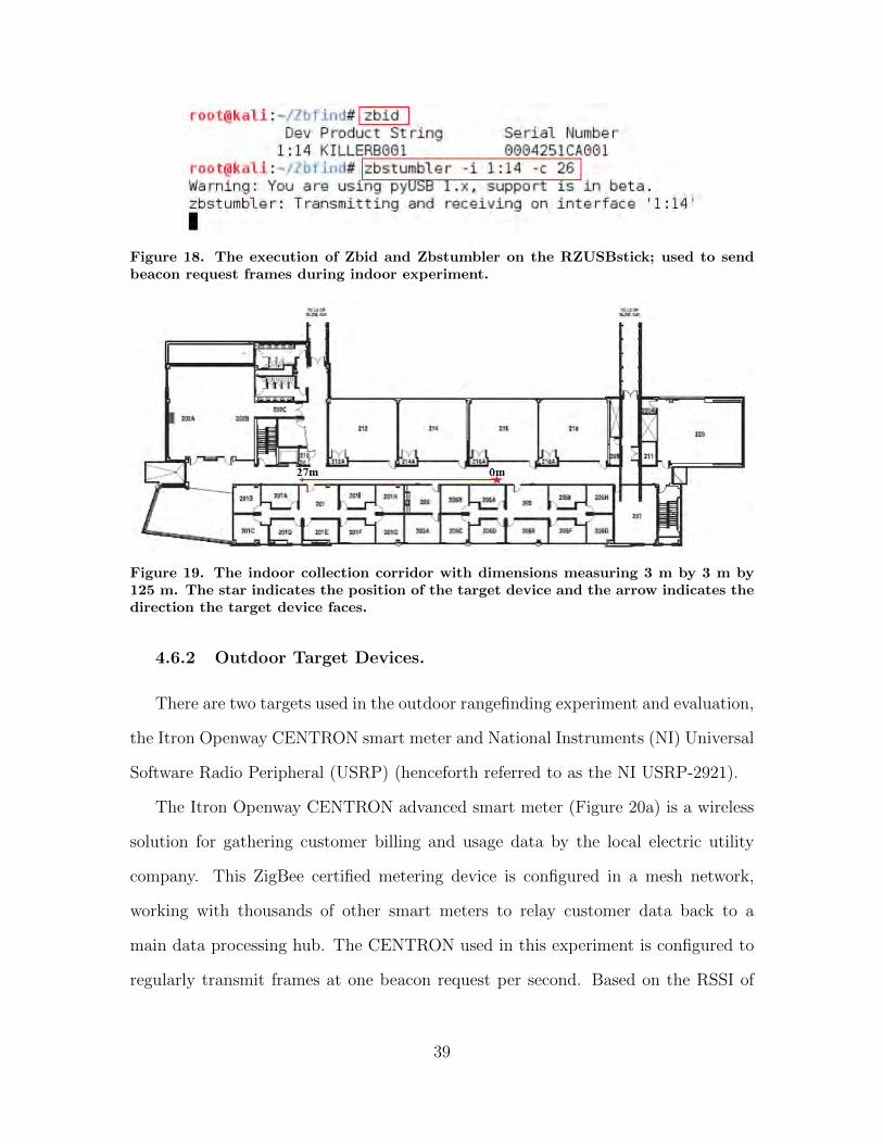
Figure 18. The execution of Zbid and Zbstumbler on the RZUSBstick; used to sendbeacon request frames during indoor experiment.

Figure 19. The indoor collection corridor with dimensions measuring 3 m by 3 m by125 m. The star indicates the position of the target device and the arrow indicates thedirection the target device faces.

4.6.2 Outdoor Target Devices.

There are two targets used in the outdoor rangefinding experiment and evaluation,

the Itron Openway CENTRON smart meter and National Instruments (NI) Universal

Software Radio Peripheral (USRP) (henceforth referred to as the NI USRP-2921).

The Itron Openway CENTRON advanced smart meter (Figure 20a) is a wireless

solution for gathering customer billing and usage data by the local electric utility

company. This ZigBee certified metering device is configured in a mesh network,

working with thousands of other smart meters to relay customer data back to a

main data processing hub. The CENTRON used in this experiment is configured to

regularly transmit frames at one beacon request per second. Based on the RSSI of

39

these beacon frames, a distance estimate is calculated and used for evaluation of each

SUT. The CENTRON used in this experiment operates on channel 26.

The NI USRP-2921 (Figure 20b) is a programmable Software Defined Radio

(SDR). In this experiment, the NI USRP-2921 is operated by the GNU Radio software

development toolkit [Rad15], a free signal processing software application designed

specifically for low-cost external RF hardware and commodity processors. The GNU

Radio includes a GUI application called GNU Radio Companion (GRC), allowing a

user to design, build, and execute software radios using a modular “block” system to

implement traditionally hardware based components.

The GNU radio blocks used to develop and transmit an IEEE 802.15.4 compliant

frame in this experiment are adapted from Bloessl [Blo12], who in turn modernized

Schmid’s [Sch06] initial contribution from 2006. The instructions for downloading,

installing, and executing both GNU Radio and Bloessl’s extended code can be found

in Appendix A. The NI USRP-2921 is connected to a laptop, via CAT-5e cable, where

the GRC software is installed. An IP address of 192.168.10.2 is given to the USRP,

and the host laptop receives the IP address 192.168.10.1. The GRC application is

then launched and executed, transmitting beacon request frames every second until

termination. A survey of 200,000 smart meters identifies the median transmission

power level to be 18.2 dBm (66.1 mW) [EPR10] with an upper value of 20.6 dBm

(114.8 mW). Based on this prior work, the USRP transmission power level is set

to 18 dBm for this experiment. The NI USRP-2921 used in this experiment comes

equipped with the Vert 2450 antenna, adding 3 dBi of gain to the radiated power

level. Calculating the added gain by the antenna, a transmission power level of 18.8

dBm (76.8 mW) is achieved. Based on the RSSI of these beacon frames, a distance

estimate is calculated and used for evaluation of each SUT. The NI USRP-2921 used

in this experiment operates on channel 26.

40

(a) Itron Openway CENTRON (b) NI USRP-2921

Figure 20. Outdoor ZigBee target devices a) Itron Openway CENTRON smart meterand b) NI USRP-2921

4.6.2.1 Outdoor Device Location.

The CENTRON smart meter is connected to the exterior side of an industrial

warehouse and adjacent to an open field, as pictured in Figure 21. The field measures

approximately 70 m by 130 m with a clear LOS between the target device and the

SUT.

The NI USRP-2921 is placed 4 m off the exterior side of a residential house and

adjacent to an open field, as pictured in Figure 22. The field measures approximately

100 m by 150 m with a clear LOS between the target device and the SUT.

41

Figure 21. The CENTRON smart meter is positioned at the 0 m marker with RSSImeasurements taken along the path of the measurement line.

Figure 22. The NI USRP-2921 is positioned at the 0 m marker with RSSI measurementstaken along the path of the measurement line.

4.6.3 Antenna Orientation and Placement.

With the exception of the NI USRP-2921, all target devices have an enclosed

and/or board printed antenna. The NI USRP-2921 uses a SMA attached Vert

2450 antenna, as pictured in Figure 20b. All target device antennas operate in an

omni-directional transmission radiation pattern.

Figure 23 shows the setup and orientation of each target device during collection

trials. Indoor target devices pictured in Figures 23a, 23c, and 23d are executed from

the top of a cardboard box, at a height of 24 cm, placed in the middle of the 3 m

hallway, and a clear LOS to the SUT. Figures 23e and 23f depict the outdoor target

device collection setup. Both outdoor targets transmit with a clear LOS to the SUT.

42

(a) Hue (b) S2 (c) MC13213

(d) RZUSBstick (e) CENTRON (f) NI USRP-2921

Figure 23. Both indoor and outdoor target device setup and orientation during collec-tion trials.

4.6.4 RSSI Samples Measured.

4.6.4.1 Indoor Environment.

RSSI measurements are taken in 2 m increments at distances d ∈ {1, 3, 5, ..., 27}m.

An increment of 2 m is used as it provides a closer interval than the 3 m interval

used in related previous work [RMLS14]. The target device is stationary at the 0 m

marker (indicated by star in Figure 19), and the SUT measures 50 RSSI samples at

each collection point for each target device. The basis for determining sample size is

the Central Limit theorem where a sample of at least 30 must be used to accurately

represent the population being sampled. Taking this into account, a value of 50 is

43

used as it provides more than enough samples for analysis. Each SUT measures 50

RSSI samples at each of the 14 collection points across all four target devices totaling

2800 RSSI measurements collected (4 ·50 ·14 = 2800). Each SUT measures 2800 RSSI

samples for a grand total of 5600 RSSI samples measured in the indoor experiment.

4.6.4.2 Outdoor Environment.

RSSI measurements are taken in 5 m increments at d ∈ {1, 6, 11, ..., 101} m. Due

to the significant increase in overall transmission distance between a target device and

SUT, the increment distance between collection points is raised to 5 m. The target

device is stationary at the 0 m marker and the SUT measures 30 RSSI samples at

each collection point for each target device. In this experiment, 30 RSSI samples are

measured compared to the 50 measured in the indoor experiment. This is due to the

increased number of collection points (14 versus 21), changing outdoor conditions,

and the minimum number of samples necessary to represent the population based on

the Central Limit theorem. Measuring 30 RSSI samples at each of the 21 collection

points across both target devices, totaling 1260 RSSI samples collected per SUT

(2 · 30 · 21 = 1260). Each SUT measures 1260 RSSI samples for a grand total of 2520

RSSI samples measured in the outdoor experiment.

4.6.5 Factors Summary.

The multiple of factors presented in the section previous are presented in a con-

densed table format below. The two environments, SUT, target devices, and the

number of RSSI measurements sampled are presented in Table 8.

44

Table 8. Summary of rangefinding experiment factors.

Factor Value

Physical LayoutIndoor

Outdoor

Tool SetZbfind & RZUSBstick

Z-Ranger & Zena

Target Device (Indoor)

HUE

S2

MC13213

RZUSBstick

Target Device (Outdoor)CENTRON

NI USRP-2921

Distance Interval (Indoor) {1, 3, 5, ..., 27} m

Distance Interval (Outdoor) {1, 6, 11, ..., 101} m

RSSI Samples Measured

5600 (Indoor)

2520 (Outdoor)

8120 (Total)

4.7 Evaluation Technique

A Lenovo ThinkPad laptop with an Intel Core i3-4000m CPU, clocked at 2.6 GHz

with 16 Gigabytes (GB) of RAM, is used during this experiment. The Lenovo runs

a 64-bit version of Windows 7 Professional with service pack one. On top of the

Windows OS, Virtual Machine (VM) Player 6.0.6 is virtualizing the Kali Linux OS,

version 2.0. From within the Kali Linux VM, both Z-Ranger and Zbfind are executed.

In order to transmit IEEE 802.15.4 frames from the NI USRP-2921 target device,

another laptop is required. For this purpose, a Hewlett Packard (HP) Envy 17 with

45

an Intel i7-720Q CPU and 16 GB of RAM running 32-bit Linux Mint 17 OS is used.

The HP Laptop is configured with USRP Hardware Driver (UHD) version 003.009

and GNU Radio Companion 3.7.8.

Direct physical measurement of signal strength from each target device is accom-

plished by each respective SUT. Measured RSSI is first converted to RSS and then

saved into a text file for each SUT at each collection point in each environment. The

collection process is the same regardless of the environment in which it is executed,

and is outlined below.

1. Position target device at 0 m marker.

2. Plug SUT into Lenovo laptop and position at 1 m marker.

3. Execute respective collection application for each SUT (Z-Ranger or Zbfind).

The collection of RSS measurement is confirmed once RSS measurement is

displayed on the Lenovo laptop screen via terminal. The measurement, along

with a packet number, is then saved for post collection analysis.

4. Apply power and/or execute required software for target device operation. The

RZUSBstick and NI USRP-2921 require the HP laptop to execute transmission.

5. Monitor SUT for the number of samples needed for experiment (50 for indoor

and 30 for outdoor). Once sample minimums are achieved, discontinue the SUT

collection and close application.

6. Discontinue target device transmission.

7. Move the SUT to next collection interval and repeat the process. Continue to

repeat the process until collection at the maximum distance (27 m for indoor

and 101 m for outdoor) is completed.

46

The CENTRON is a fully functioning smart meter and not permitted to be pow-

ered off or moved. Due to this limitation, Step 1 and 6 are not executed during this

collection trial for the CENTRON data collection. All data is collected in the re-

spective environments, and no RSSI values are simulated. The following subsections

describe the specific collection process details for each environment.

4.7.1 Indoor Evaluation.

The corridor is marked off in 2 m increments, out to a maximum of 27 m as

shown in Figure 24a. The Lenovo and SUT are perched on top of a rolling arm chair,

measuring 63 cm in height and positioned at the 1 m marker. Figure 24b presents the

positioning of the target devices and SUT. The S2 is plugged into an outlet measuring

42 cm in height at the 0 m marker. The remaining three targets are positioned on

top of a cardboard box measuring 24 cm in height, also at the 0 m marker. After

RSSI sample measurement is completed at the 1 m marker, the SUT is rolled to the

next interval marker and the collection process repeats.

4.7.2 Outdoor Evaluation.

Figure 25a shows the Lenovo and connected SUT as held during the experiment

at a height of 1 m. Both targets are stationary at the 0 m marker throughout

the collection experiment. Markers are set at 5 m intervals out to a maximum of

101 m. Initial collection starts with the SUT set at the 1 m marker, measuring

30 RSSI samples. Once finished, the SUT is moved to the next increment and the

process is repeated. Figure 25b shows the NI USRP-2921 target device setup. The

NI USRP-2921 is placed on top the HP laptop that is positioned on top of a stool,

measuring 1 m in height. The CENTRON is affixed to an exterior warehouse wall at

a height of 1.5 m.

47

(a) Office corridor (b) Indoor collection setup

Figure 24. Indoor RSSI sample measurement setup.

(a) SUT Collection (b) Target Device

Figure 25. Outdoor RSSI sample measurement setup.

4.8 K-fold Cross-Validation

Unlike Zbfind, Z-Ranger has no initial P or A parameter. For initial distance

calculations the P parameter for Z-Ranger is borrowed from Zbfind and set to P = 3.0.

The A parameter must be found empirically since it is unique to each transceiver.

Observing the transmission power levels of the indoor and outdoor targets used in

this research, it can be concluded that indoor devices operate at lower transmission

power levels than outdoor devices, thus a different A parameter is required for each

48

environment. To establish an A parameter, the K -fold cross-validation method is

used.

Figure 26 presents a diagram illustrating the K-fold cross-validation process for

training and testing data sets. The K-fold cross-validation method randomly [Ran15]

splits a limited data set into K mutually exclusive folds, without using replacement

[Koh95]. The folds are randomly chosen and stratified, as this lessens the chance of

producing a biased estimate of accuracy [Koh95]. The folds are then divided into

two groups, one for testing data and one for training data. The training group is

comprised of K − 1 folds and the testing group is comprised of the remaining Kth

fold. The training group is then compared to the testing group and the amount of

error produced is quantified using (3), this completes one round of testing. This

process is repeated K times in order to incorporate all folds into each group; thus,

a user is able to train and test using the entire data set. After all K rounds are

completed, the training group value that produces the least amount of MAPE is used

for the A parameter in (2). Since all data is incorporated into training and testing,

model overfitting is limited, producing a more accurate model to use [Koh95].

4.8.1 Indoors.

All RSS samples recovered at d = 1 m for all four target devices are grouped

together, resulting in a group of 200 samples. The samples are then randomly divided

into five mutually exclusive folds containing 40 samples each. Table 9 depicts the five

randomly chosen folds from the 200 samples and the corresponding average RSS

sample values.

49

Figure 26. K-fold cross-validation technique used to discover the A parameter forZ-Ranger [Koh95].

The training group is formed by combining four of the five folds and averaging the

RSS values together. The five training folds, associated RSS, testing fold, and asso-

ciated MAPE are presented in Table 10. The RSS value of −43.46 dBm, originating

from the combination of folds {5, 1, 2, 3}, is chosen as the initial indoor A parameter

for Z-Ranger, as it offers the best indicator of future performance with MAPE at

M = 0.06%.

50

Table 9. Five indoor folds and corresponding average RSS samples for Z-Ranger.

Fold Number Avg RSS (dBm)1 -43.292 -43.133 -44.024 -43.495 -43.41

Table 10. 5-fold cross-validation for indoor Z-Ranger A parameter.

Train folds Train RSS (dBm) Test fold Test RSS (dBm) MAPE

1, 2, 3, 4 -43.48 5 -43.41 0.18%

2, 3, 4, 5 -43.51 1 -43.29 0.51%

3, 4, 5, 1 -43.55 2 -43.13 0.97%

4, 5, 1, 2 -43.33 3 -44.02 1.57%

5, 1, 2, 3 -43.46 4 -43.49 0.06%

4.8.2 Outdoors.

All RSS samples from both outdoor targets at d = 1 m are grouped together,

resulting in a pool of 60 samples. The value of K = 3 is used due to the decreased

sample size for outdoor targets (60 outdoor versus 200 indoor). The group is then

subdivided into three folds of 20 RSS samples each. Table 11 presents the averaged

RSS values for each of the three mutually exclusive folds used for cross-validation.

In the same fashion as used above, the training groups are formed by combining

two folds and averaging the RSS values together. The three training groups, associ-

ated RSS, testing group, and associated MAPE is presented in Table 12. The RSS

value of −39.55 dBm, originating from folds {1 and 2}, is chosen as the initial outdoor

A parameters for Z-Ranger as it offers the best indicator of future performance with

MAPE M = 0.51%.

51

Table 11. Three outdoor folds and corresponding average RSS samples for Z-Ranger.

Fold Number Avg RSS (dBm)1 -40.432 -38.673 -39.35

Table 12. 3-fold cross validation for outdoor Z-Ranger A parameter.

Train folds Train RSS (dBm) Test folds Test RSS (dBm) MAPE

1 and 2 -39.55 3 -39.35 0.51%

2 and 3 -39.00 1 -40.43 3.53%

3 and 1 -39.89 2 -38.67 3.17%

4.9 Summary

This IEEE 802.15.4 rangefinding and evaluation experiment is conducted in both

indoor and outdoor environments, against an array of target devices. Varying fac-

tors include LR-WPAN sensor targets, antenna type, and executing software. The

methodology outlined in this chapter presents an experiment that measures 50 RSSI

samples at 14 collection points from four different targets by two different tool sets

in an indoor environment. The experiment continues outside, measuring 30 RSSI

samples at 21 collection points against two different targets using the same two tool

sets under test.

52

V. Results and Analysis

In this chapter distance estimates are calculated based on recovered RSS samples

from Chapter IV. Comparing actual distance to estimated distance, a corresponding

MAPE value is produced for each SUT at each collection point. A 99% CI is then

calculated for each SUT using the recovered MAPE values. Analysis of each SUT is

presented and further refinements are presented.

5.1 Initial Tool Set Comparison

5.1.1 Indoors.

5.1.1.1 Z-Ranger.

The A parameter derived from the cross-validation method in Chapter IV,

A = −43.46, and borrowing P = 3.0 from the Zbfind tool set a distance estimate

is calculated at each collection interval d ∈ {1, 3, 5, ..., 27} m using (2). Table 13

presents the estimated distance, absolute error percentage, MAPE per device, and

average MAPE for the tool set.

Average MAPE across all four targets is M = 54.00% with the lowest MAPE value

of M = 45.87%, found while rangefinding the S2 target. The highest MAPE value of

M = 66.67% is produced while rangefinding the Hue target. With the exception of

the S2, which is plugged into the wall, all three targets produce the most amount of

error at the 27 m collection point with an average MAPE of M = 78.77%. This spike

in MAPE may be the result from multi-path fading due to the location of the target

devices in the middle of the corridor.

53

Table 13. Indoor distance estimates and corresponding MAPE produced by Z-Rangerusing the values of A = −43.46 and P = 3.0.

Hue S2 MC13213 RZUSBstickDst Est Dst MAPE Est Dst MAPE Est Dst MAPE Est Dst MAPE1m 0.53m 47.4% 0.97m 21.2% 1.22m 21.8% 1.60m 60.4%3m 1.13m 62.2% 2.24m 25.2% 1.70m 43.2% 3.91m 30.2%5m 1.30m 74.1% 1.91m 61.8% 2.50m 49.9% 4.68m 6.4%7m 1.22m 82.6% 1.57m 77.5% 2.29m 67.3% 3.62m 48.3%9m 1.46m 83.8% 1.88m 79.1% 3.03m 66.3% 10.61m 17.9%11m 9.02m 18.0% 7.46m 32.3% 7.09m 35.6% 11.72m 6.5%13m 7.02m 46.0% 5.53m 57.5% 4.06m 68.8% 4.08m 68.6%15m 4.07m 72.8% 6.71m 55.3% 8.11m 45.9% 5.37m 64.2%17m 8.11m 52.3% 9.42m 44.6% 5.98m 64.8% 5.52m 67.5%19m 3.83m 79.9% 6.10m 67.9% 8.15m 57.1% 7.74m 59.3%21m 4.32m 79.4% 11.31m 46.2% 7.10m 66.2% 7.44m 64.6%23m 5.88m 74.5% 15.23m 33.8% 6.57m 71.4% 14.09m 38.7%25m 6.36m 74.5% 15.79m 36.8% 11.49m 54.1% 11.71m 53.1%27m 3.82m 85.8% 21.20m 21.5% 6.28m 76.7% 7.07m 73.8%

MAPE=66.66% MAPE=45.87% MAPE=56.37% MAPE=47.11%Average MAPE over all four targets=54.00%

5.1.1.2 Zbfind.

Using (2) and the Zbfind original values of A = −58.0 and P = 3.0, a distance

estimate is calculated at each collection interval d ∈ {1, 3, 5, ..., 27} m. An absolute

error value is also calculated at each collection point. The second to last row of Table

14 presents the MAPE over all collection points and the last row presents the average

MAPE produced by the four target devices during indoor collection.

The average MAPE produced by all four target during indoor rangefinding is

M = 70.22%. The Hue device produced the highest MAPE value at M = 86.63%.

This may be due to poor or degraded signal strength as the Hue also produced the

most MAPE during Z-Ranger collection. The least amount of MAPE produced comes

while rangefinding the S2 target device with M = 58.54%. The S2 also produced the

least amount of MAPE during Z-Ranger rangefinding.

54

Table 14. Indoor distance estimates and corresponding MAPE produced by Zbfindusing the parameters of A = −58.0 and P = 3.0.



5.1.1.3 Summary Analysis.

A 99% CI is calculated from the MAPE produced for each target device and

presented in Figure 27.

There is no significant difference between Z-Ranger and Zbfind when rangefinding

the Hue (Z-Ranger: M = 66.66%, SD = 19.34%; Zbfind: M = 86.63%, SD = 8.19%),

S2 (Z-Ranger: M = 45.87%, SD = 22.11%; Zbfind: M = 58.54%, SD = 18.76%),

MC13213 (Z-Ranger: M = 56.37%, SD = 15.54%; Zbfind: M = 77.06%, SD =

18.02%), and the RZUSBstick (Z-Ranger: M = 47.11%, SD = 23.3%; Zbfind: M =

58.63, SD = 16.6%) target devices, p ≥ .01.

Results from the indoor trials do not suggest any significant functional differences

in rangefinding error between the two tool sets for indoor warwalking.

55

Figure 27. This figure depicts the MAPE produced by Z-Ranger during indoorrangefinding using parameters discovered from the cross-validation method. TheMAPE produced by Zbfind is the result of using original values.

5.1.2 Outdoors.

5.1.2.1 Z-Ranger.

The A parameter derived from the cross-validation parameter discovery method,

A = −39.55, coupled with P = 3.0 from the Zbfind tool set, a distance estimate

is calculated at each collection interval d ∈ {1, 6, 11, ..., 101} m using (2). Table 15

presents the estimated distance, absolute error percentage, MAPE per device, and

overall MAPE for the tool set.

While rangefinding the NI USRP-2921 target, a MAPE value of M = 88.32%

is recorded, the highest of the two outdoor targets. The MAPE produced while

rangefinding the CENTRON target sensor is M = 70.20%, with an average MAPE

of M = 79.26% between the two target devices.

56

Table 15. Outdoor distance estimates and corresponding MAPE produced by Z-Rangerusing the parameters of A = −39.55 and P = 3.0.

NI USRP-2921 CENTRONDst Est Dst MAPE Est Dst MAPE1m 0.71m 29.5% 1.39m 39.4%6m 0.79m 86.8% 1.86m 69.1%11m 1.06m 90.4% 2.52m 77.1%16m 1.30m 91.9% 3.13m 80.5%21m 1.41m 93.3% 7.43m 64.6%26m 1.44m 94.4% 11.50m 55.8%31m 1.66m 94.6% 10.81m 65.1%36m 2.09m 94.2% 13.94m 61.3%41m 2.72m 93.4% 9.06m 77.9%46m 3.56m 92.3% 17.00m 63.0%51m 3.81m 92.5% 12.98m 74.6%56m 3.54m 93.7% 14.01m 75.0%61m 4.80m 92.1% 9.76m 84.0%66m 7.15m 89.2% 13.28m 79.9%71m 6.96m 90.2% 20.57m 71.0%76m 5.49m 92.8% 16.73m 78.0%81m 4.60m 94.3% 30.51m 62.3%86m 10.22m 88.1% 19.03m 77.9%91m 14.56m 84.0% 22.99m 74.7%96m 6.93m 92.8% 28.82m 70.0%101m 15.75m 84.4% 27.14m 73.1%

MAPE=88.32% MAPE=70.20%Average MAPE for both targets=79.26%

5.1.2.2 Zbfind.

Using (2) and the Zbfind original values of A = −58.0 and P = 3.0, a distance

estimate is calculated at each collection interval d ∈ {1, 6, 11, ..., 101} m. An absolute

error value is also calculated at each collection point. The second to last row of

Table 16 presents the MAPE over all collection points and the last row presents the

average MAPE produced by both target devices during outdoor collection. While

rangefinding outdoor targets, MAPE produced by Zbfind is M = 98.01% for the NI

USRP-2921 and M = 87.33% for the CENTRON smart meter. An average MAPE

of M = 92.67% for both targets.

57

Table 16. Outdoor distance estimates and corresponding MAPE produced by Zbfindusing the parameters of A = −58.0 and P = 3.0.

NI USRP-2921 CENTRONDst Est Dst MAPE Est Dst MAPE1m 0.05m 95.1% 0.41m 58.9%6m 0.22m 96.3% 1.03m 82.8%11m 0.27m 97.5% 1.95m 82.3%16m 0.30m 98.1% 1.74m 89.1%21m 0.33m 98.4% 2.93m 86.1%26m 0.33m 98.7% 3.95m 84.8%31m 0.40m 98.7% 5.17m 83.3%36m 0.40m 98.9% 4.14m 88.5%41m 0.54m 98.7% 5.98m 85.4%46m 0.74m 98.4% 3.77m 91.8%51m 0.70m 98.6% 4.97m 90.2%56m 0.66m 98.8% 6.12m 89.1%61m 0.71m 98.8% 6.12m 90.0%66m 1.30m 98.0% 5.33m 91.9%71m 1.89m 97.3% 7.47m 89.5%76m 1.55m 98.0% 6.12m 91.9%81m 1.57m 98.1% 7.24m 91.1%86m 1.95m 97.7% 6.61m 92.3%91m 1.61m 98.2% 7.64m 91.6%96m 2.11m 97.8% 7.59m 92.1%101m 2.11m 97.9% 8.84m 91.2%



A 99% CI is calculated from the MAPE produced for each target device and

presented in Figure 28. Analysis concludes there is a significant reduction in MAPE

produced by Z-Ranger while rangefinding the USRP NI-2921 (M = 88.32%, SD =

13.85%) and CENTRON (M = 70.20%, SD = 10.24%) targets, as compared to

Zbfind for the NI USRP-2921 (M = 98.01%, SD = .90%) and CENTRON (M =

87.33%, SD = 7.30%) targets, p ≤ .01.

Outdoor results suggest a statistically significant reduction in MAPE when Z-Ranger

is used versus Zbfind (p ≤ .01).

58

Figure 28. This figure depicts the MAPE produced by Z-Ranger during outdoorrangefinding using parameters discovered from the cross-validation method. TheMAPE produced by Zbfind is the result of using original values.

5.2 Best fit Parameter Refinement

The Z-Ranger tool set outperforms Zbfind during outdoor collection trials only.

The relatively high MAPE results suggest a penetration tester may still have a difficult

time in locating outdoor devices and an even more difficult assignment locating indoor

devices. Calibration of both the A and P value used in (2) may be necessary to achieve

a more accurate rangefinding tool set.

An alternative to the cross-validation method of parameter discovery is to identify

the best overall A and P parameters that produce the least amount of MAPE over

all collection points. The corresponding A and P parameters can then be averaged

together across all target devices in each respective environment (indoor or outdoor).

This produces a versatile combination of A and P parameters that can be used as

“default” parameters when rangefinding unknown devices. Rappaport identifies com-

mon path-loss values for differing environments [Rap96] and these are presented in

Table 17.

59

Table 17. Identified path-loss exponents from different environments. Adapted from[Rap96].

Environment Path Loss ValuesFree Space 2

Urban area cellular radio 2.7 to 3.5Shadowed urban cellular radio 3 to 5

In building line-of-sight 1.6 to 1.8Obstructed in building 4 to 6Obstructed in factories 2 to 3

Based on the previous work by Rappaport [Rap96], adjustment of the P parameter

between a range of 1.6−4.0, at increments of 0.1 is conducted. The range selected for

P is chosen to encompass many different propagation environments, even though these

experiments are conducted in an office corridor and an outdoor open field, both with

an established LOS. This range allows for uncontrolled factors to be compensated

for and thus not overlook the most advantageous P parameter. The A parameter

is set at −65 dBm and increments towards 19 dBm until the lowest MAPE value is

observed. This range for the A parameter is chosen as it encompasses all transmission

power levels of the target devices used in this study. The A parameter, along with the

P parameter under test, is then applied to (2) and a distance estimate is produced

at each collection point interval. A corresponding MAPE value is calculated over

all collection points for each device. Identification of the corresponding A and P

parameters that produce the least amount of overall MAPE is identified.

This process is executed for each device in each respective environment. The

corresponding A and P parameters that produce the least amount of MAPE are then

averaged across all devices for each respective environment. This produces default A

and P parameters for each environment. This process is repeated for both Z-Ranger

and Zbfind tool sets and is referred to as the best fit parameter discovery method.

60

5.2.1 Indoors.

5.2.1.1 Z-Ranger.

Using the process described in Section 5.2, the P, the A, and calculated MAPE

over all indoor collection points is found for the Z-Ranger tool set and presented in

Table 18. The full range of parameters can be found in Appendix B. Each best fit P

parameter is listed in the second column, followed by the corresponding A parameter,

and MAPE is presented in column four. The parameters are then averaged and

presented in the last row. The indoor best fit parameters for Z-Ranger are A = −38.93

and P = 2.75.

Table 19 presents the four indoor targets evaluated using the best fit parameters

of A = −38.93 and P = 2.75. In Table 19, a distance estimate is calculated at each

collection point, along with a corresponding MAPE value. MAPE for each device

over all collection points and average MAPE across all four devices is calculated and

presented in the bottom two rows.

The average MAPE produced across all four targets is M = 44.56%. Comparing

Table 19 to the initial rangefinding figures in Table 13, the S2 device still produces the

least amount of MAPE with M = 31.72%, a reduction of 30.9%. The highest amount

of MAPE is produced while rangefinding the RZUSBstick with 58.64%, counter to

the previous MAPE value of 47.11% identified in Table 13.

61

Table 18. Best fit P and corresponding A parameters for the Z-Ranger tool set. TheBest fit P and A parameters displayed are found to produce the least amount of MAPEfor each indoor target device.

Device P A (dBm) MAPEHue 3.5 -27.7 41.13%S2 2.8 -40.4 29.13%MC13213 2.6 -38.0 31.13%RZUSBstick 2.1 -49.6 46.17%Averaged best fit parameters, A = −38.93 and P = 2.75

Table 19. Indoor distance estimates and corresponding MAPE produced by Z-Rangerusing the parameters of A = −38.93 and P = 2.75.



5.2.1.2 Zbfind.

Using the best fit method described above, new recommended default P and A

parameters for Zbfind are found and presented in Table 20. Best fit parameters for

the Zbfind tool set are found to be P = 2.25 and A = −49.33.

Table 21 presents the four indoor targets evaluated using the new best fit param-

eters of A = −49.33 and P = 2.25. Table 21 presents the distance estimate at each

collection point, along with a corresponding MAPE value. MAPE for each device

62

Table 20. The best fit P and corresponding A parameters for the Zbfind tool set. Thebest fit P and A parameters displayed are found to produce the least amount of MAPEfor each indoor target device.

Device P A (dBm) MAPEHue 2.8 -32.8 33.87%S2 2.0 -59.0 31.06%MC13213 2.1 -46.8 37.88%RZUSBstick 2.1 -58.7 33.00%Averaged best fit parameters, A = −49.33 and P = 2.25

Table 21. Indoor distance estimates and corresponding MAPE produced by Zbfindusing the parameters of A = −49.33 and P = 2.25.


MAPE=65.45% MAPE=76.96% MAPE=47.05% MAPE=84.15%Total MAPE over all four targets=68.33%

over all collection points and average MAPE across all four devices is calculated in

the bottom two rows.

The average MAPE produced across all four targets is M = 68.33%. Comparing

MAPE values from Table 21 to the previous MAPE figures in Table 14, a reduction

in average MAPE by 2.68% is achieved using the best fit parameters found herein.

63

Figure 29. This figure depicts the MAPE produced by Z-Ranger and Zbfind duringindoor rangefinding using parameters discovered from the best fit method.


A 99% CI is calculated from the MAPE produced for each target device and pre-

sented in Figure 29. Analysis concludes there is not a significant difference in MAPE

produced by Z-Ranger when rangefinding any of the indoor targets using the best fit

method. The Hue (M = 51.86%, SD = 22.07%), S2 (M = 31.66%, SD = 21.02%),

MC13213 (M = 36.06%, SD = 21.69%), and RZUSBstick (M = 58.63%, SD =

41.95%) targets produced no significant difference in MAPE as compared to Zbfind

for the Hue (M = 65.44%, SD = 15.79%), S2(M = 76.96%, SD = 61.55%), MC13213

(M = 47.05%, SD = 19.18%), and RZUSBstick (M = 84.15%, SD = 69.58%) tar-

gets, p ≥ .01.

With no significant reduction in MAPE produced by Z-Ranger during the indoor

rangefinding experiment, it can be concluded that a higher RSSI resolution does not

reduce mean distance estimation error. Therefore, the hypothesis is not supported

by these results.

64

5.2.2 Outdoors.

5.2.2.1 Z-Ranger.

Using the best fit method described above, the recommended default parameters

of A = −26.2 and P = 2.5 are found for the two outdoor target devices. Table 22

presents all the calibrated A parameters for the range of P values under test. The

corresponding MAPE over all collection points is presented in columns three and five.

Table 23 presents the distance estimates produced at each collection point for each

outdoor target. Corresponding MAPE is also calculated at each collection point, with

an average MAPE of M = 71.85% presented in the final row of Table 23.

65

Table 22. Best fit P and corresponding A parameters for the Z-Ranger tool set. TheBest fit P and A parameters displayed are found to produce the least amount of MAPEfor each outdoor target device.

Device P A (dBm) MAPECENTRON 2.3 -36.4 31.82%NI USRP-2921 2.7 -16.0 54.34%Averaged Best-fit parameters, A = −26.2 and P = 2.5

Table 23. Outdoor distance estimates and corresponding MAPE produced by Z-Rangerusing best fit parameters of A = −26.2 and P = 2.5.

CENTRON NI USRP-2921Dst Est Dst MAPE Est Dst MAPE1m 5.09m 409.2% 2.25m 124.9%6m 7.18m 19.6% 2.59m 56.8%11m 10.35m 5.9% 3.66m 66.7%16m 13.44m 16.0% 4.69m 70.7%21m 37.94m 80.7% 5.18m 75.4%26m 64.06m 146.4% 5.32m 79.5%31m 59.52m 92.0% 6.28m 79.7%36m 80.72m 124.2% 8.27m 77.0%41m 48.13m 17.4% 11.37m 72.3%46m 102.47m 122.8% 15.70m 65.9%51m 74.11m 45.3% 17.02m 66.6%56m 81.21m 45.0% 15.60m 72.1%61m 52.62m 13.7% 22.49m 63.1%66m 76.20m 15.5% 36.25m 45.1%71m 128.80m 81.4% 35.11m 50.5%76m 100.51m 32.3% 26.39m 65.3%81m 206.72m 155.2% 21.32m 73.7%86m 117.27m 36.4% 55.62m 35.3%91m 147.14m 61.7% 85.05m 6.5%96m 193.01m 101.1% 34.92m 63.6%101m 179.61m 77.8% 93.49m 7.4%


5.2.2.2 Zbfind.

The best fit method is also applied to the Zbfind dataset. After completing the

calculations, the default parameters of A = −29.4 and P = 2.35 are found for the

two outdoor target devices. Table 24 presents the calibrated P and corresponding A

66

Table 24. Best fit P and corresponding A parameters for the Zbfind tool set. The bestfit P and A parameters displayed are found to produce the least amount of MAPE foreach outdoor target device.

Device P A (dBm) MAPECENTRON 2.0 -45.9 17.66%NI USRP-2921 2.7 -12.9 28.80%Averaged best fit parameters, A = −29.4 and P = 2.35

parameters under test. The calculated MAPE over all collection points is presented

in columns three and five.

Table 25 lists the distance estimates produced at each collection point for each

outdoor target using the best fit parameters found in Table 24. Corresponding MAPE

is calculated at each collection point with a combined MAPE presented in the final

row of Table 25.

MAPE produced while rangefinding the CENTRON smart meter is M = 191.0%,

an increase of 54.3% over the initial MAPE value of M = 87.3% presented in Table

16. Rangefinding the NI USRP-2921 produced a MAPE value of M = 72.2%, a

reduction of 35.8% over the initial MAPE value of M = 98.0%. Average MAPE for

both devices is M = 131.6%, an increase of 29.6% over the initial average MAPE

value of M = 92.7%, as presented in Table 16.


A 99% CI is calculated from the MAPE produced for each target device and pre-

sented in Figure 30. Analysis concludes there is a significant difference in MAPE pro-

duced by Z-Ranger when rangefinding the CENTRON (M = 81.08%, SD = 90.45%)

target, as compared to Zbfind for the CENTRON (M = 190.94%, SD = 84.00%)

target, p ≤ .01.

There is no significant difference in MAPE for Z-Ranger when rangefinding the

NI USRP-2921 (M = 62.78%, SD = 25.17%) target, as compared to Zbfind for the

67

Table 25. Outdoor distance estimates and corresponding MAPE produced by Zbfindusing best fit parameters of A = −29.4 and P = 2.35.

CENTRON NI USRP-2921Dst Est Dst MAPE Est Dst MAPE1m 5.29m 428.9% 0.35m 64.5%6m 17.14m 185.7% 2.37m 60.5%11m 38.66m 251.4% 3.07m 72.1%16m 33.37m 108.6% 3.45m 78.5%21m 64.98m 209.4% 3.87m 81.6%26m 95.22m 266.2% 3.94m 84.8%31m 134.17m 332.8% 4.92m 84.1%36m 100.98m 180.5% 4.96m 86.2%41m 161.63m 294.2% 7.22m 82.4%46m 89.78m 95.2% 10.69m 76.8%51m 127.76m 150.5% 10.00m 80.4%56m 166.45m 197.2% 9.17m 83.6%61m 166.45m 172.9% 10.10m 83.4%66m 139.53m 111.4% 21.54m 67.4%71m 214.74m 202.5% 34.47m 51.4%76m 166.45m 119.0% 26.86m 64.7%81m 206.49m 154.9% 27.38m 66.2%86m 183.58m 113.5% 35.82m 58.3%91m 221.15m 143.0% 28.18m 69.0%96m 218.99m 128.1% 39.43m 58.9%101m 266.40m 163.8% 39.43m 61.0%


NI USRP-2921 (M = 72.18%, SD = 10.78%), p ≥ .01.

The significant difference in MAPE produced by Z-Ranger is observed during 50%

of the outdoor rangefinding experiment. However, the reduction in MAPE shown

by Z-Ranger is not consistent and therefore does not support the hypothesis that

configured distance estimating parameters, along with an increased RSSI resolution,

reduces MAPE produced.

68

Figure 30. This figure depicts the MAPE produced by Z-Ranger and Zbfind duringoutdoor rangefinding using parameters discovered from the best fit method.

5.3 RSS Windowing

An alternative method for improving distance estimation may be to take the

mean of multiple RSS measurements and calculate a distance estimate from this

value. This process is then repeated as new RSS measurements are taken. Since

signals propagate, deflect, and refract off objects, walls, and other obstructions, it is

posited that by taking the mean of two or three RSS measurements, a more accurate

representation of signal strength can be obtained. Therefore, a distance calculation

based on this mean RSS value can more accurately reflect the true distance between

transceivers. This method is commonly referred to as windowing.

In this section, two types of windowing are examined: a sliding and a sequential

window.

• A sliding window is the mean of multiple RSS measurements based on the

size on a designated window. Once a new RSS measurement is taken, the

window slides to incorporate the new measurement into the mean and pushes

the first RSS measurement out. This method of replacement is referred to as the

First In Last Out (FILO) method. This slide allows the window to continually

69

incorporate new RSS measurements into the mean RSS product. The sliding

window method reuses each RSS measurement and the amount of reuse is based

on the designated window size.

• Sequential windowing takes the mean of multiple RSS measurements based on

the size of the window. Once enough new RSS measurements are taken to fill

the next window, a new mean RSS value is found. This method uses each RSS

measurement only once and must wait until the window is “filled” again before

producing a new mean RSS value.

Two window sizes of each type are examined. Results are quantified based on

the amount of MAPE produced by each tool set over all collection points, similar

to the experiments presented previously. The A and P parameters used for distance

calculations are the parameters discovered from the best fit method, presented in

Section 5.2.

5.3.1 Indoor RSS Sliding Window.

5.3.1.1 Z-Ranger.

Table 26 presents the MAPE produced over all collection points for each indoor

target device. A comparison between the best-fit, two-, and three-window methods

finds a slight improvement with the sliding two-window method, yielding an average

MAPE reduction of 4.2% when compared to the average MAPE value of 44.56%, as

identified in Table 19.

70

Table 26. Indoor RSS sliding window MAPE comparison for Z-Ranger.

Method Hue S2 MC13213 RZUSBstick MAPE Improvement

Best-fit 51.86% 31.67% 36.06% 58.64% 44.56% -

two-Window 51.97% 26.29% 33.10% 59.39% 42.69% 4.2%

three-Window 52.03% 26.98% 33.09% 59.36% 42.87% 3.8%

This window simulation process is repeated, in the same fashion as above, for all

sliding and sequential windowing scenarios. Full windowing tables are presented in

Appendix C.

5.3.2 RSS Windowing Results.

Examining the overall results from the RSS windowing experiment for Z-Ranger,

in only two instances did windowing outperform the best fit method; the indoor sliding

two-window and the indoor sequential two- and three-window. The indoor sliding

two-window (Table 26) average MAPE is found to be reduced by 4.2%. Similarly, by

using the indoor sequential two- and three-window method (Table 41) average MAPE

is reduced by 2.8%. The success of these results is limited to this simulation and is

not incorporated into the Z-Ranger application due to the inconsistency in reducing

MAPE production.

Examining the overall results for Zbfind, it is found windowing did not produce

significant improvement in the average MAPE. In every case, the best fit method

produced the least amount of average MAPE for the tool set.

71

5.4 Z-Ranger Implementation

5.4.0.1 Indoor Parameter Discovery Comparison.

Table 27 provides a summary and comparison of the A and P parameters found

from both the cross-validation and best fit methods of parameter discovery for Z-Ranger

during the indoor experiment. A 99% CI is calculated from the MAPE produced while

rangefinding each target device and presented in Figure 31.

Analysis suggests there is no significant difference while rangefinding the Hue

(M = 51.86%, SD = 22.07%), S2 (M = 31.66%, SD = 21.02%), MC13213 (M =

36.06%, SD = 21.69%), and RZUSBstick (M = 58.63%, SD = 41.95%) targets us-

ing the best fit method, as compared to the cross-validation method for the Hue

(M = 66.66%, SD = 19.34%), S2(M = 45.87%, SD = 22.11%), MC13213 (M =

56.37%, SD = 15.54%), and RZUSBstick (M = 47.11%, SD = 23.30%) targets,

p ≥ .01.

The results from the parameter discovery comparison marginally favor the best fit

method over the cross-validation method. This conclusion suggests the parameters

of A = −38.93 and P = 2.75 offer the most versatility for indoor rangefinding, and

thus are hard coded into the final version of Z-Ranger.

72

Table 27. Z-Ranger log-distance path loss parameter discovery method comparison foran indoor environment.

Cross-Validation Best fitP A (dBm) MAPE P A (dBm) MAPE

Indoor 3.0 -43.46 54.00% 2.75 -38.93 44.56%

Figure 31. This figure depicts the MAPE produced by Z-Ranger during indoorrangefinding using parameters discovered from both the cross-validation and best fitlog-distance path loss parameter discovery methods.

5.4.0.2 Outdoor Parameter Discovery Comparison.

Table 28 provides a summary and comparison of the A and P values found from

both the cross-validation and best fit parameter discovery methods for the Z-Ranger

tool set during the outdoor experiment. A 99% is calculated from the MAPE produced

while rangefinding each target device and presented in Figure 32. Analysis concludes

there is a significant reduction in MAPE produced by Z-Ranger when rangefinding the

NI USRP-2921 using the best fit method (M = 62.78%, SD = 25.17%) as compared

to the cross-validation method (M = 88.32%, SD = 3.02%), p ≤ .01.

There was no significant difference while rangefinding the CENTRON (M =

81.08%, SD = 90.45%) target using the best fit method, as compared to the cross-validation

73

Table 28. Z-Ranger log-distance path loss parameter discovery method comparison foran outdoor environment.

Cross-Validation Best-fitP A (dBm) MAPE P A (dBm) MAPE

Outdoor 3.0 -39.55 79.26% 2.50 -26.20 71.85%

Figure 32. This figure depicts the MAPE produced by Z-Ranger during outdoorrangefinding using parameters discovered from both the cross validation and best fitparameter discovery methods.

method for the CENTRON (M = 70.20%, SD = 10.24%) target, p ≥ .01.

Although the best fit method did not consistently outperform the cross-validation

method, it did present a reduced MAPE value against the NI USRP-2921 target

and thus the parameters discovered from the best fit method are chosen for final

implementation into the Z-Ranger application.

The Z-Ranger application requires default parameters for use during both indoor

and outdoor rangefinding exercises. Based on the evidence presented previously,

the A and P parameters discovered using the best fit method are chosen for final

implementation in the application. The indoor and outdoor default parameters for

Z-Ranger are A = −38.93 and P = 2.75, and A = −26.2 and P = 2.50.

The individual best fit parameters found in Table 18 and Table 22 are also included

in the final version of the Z-ranger application. These parameters are displayed via the

74

terminal when a penetration tester adds the -r option to the ./z-ranger command,

indicating she would like to manually enter the A and P parameters used for distance

calculation. Figure 33 and Figure 34 present examples of the releasable open source

version of Z-Ranger targeting a RZUSBstick while indoors and a NI USRP-2921 while

outdoors.

Individualized A and P parameters produce the least amount of MAPE out of

all methods discussed in this Thesis. Additional discovery of A and P parameters

for other devices not studied herein can be added to future versions of the Z-Ranger

application.

75

Figure 33. Example execution of Z-Ranger rangefinding a RZUSBstick indoors.

Figure 34. Example execution of Z-Ranger rangefinding a NI USRP-2921 outdoors.

76

5.5 Production Tool Set Comparison

The final version of Z-Ranger is available with open source code [Sei16] and is pre-

sented at the 2016 International Conference on Cyber Warfare and Security (ICCWS)

[SRMR16]. As such, a comparison of Zbfind to Z-Ranger using only default settings

provides insight as to what a novice user would encounter while rangefinding select

target devices. Figure 35 depicts Z-Ranger and Zbfind rangefinding the indoor target

devices using their respective default log-distance path loss parameters of A = −38.93

and P = 2.75 for Z-Ranger and A = −58.0 and P = 3.0 for Zbfind. Z-Ranger is found

to significantly decrease MAPE in three of the four rangefinding estimates (Hue, S2,

and MC13213 target devices). Only the RZUBstick (M = 58.63%, SD = 41.95%)

shows no significant reduction in MAPE, as compared to Zbfind for the RZUSBstick

(M = 58.62%, SD = 16.59%), p ≥ .01. This accuracy improvement is also supported

when examining average MAPE across all four targets by both SUT. The average

MAPE produced by Zbfind is M = 70.21% and Z-Ranger produces M = 44.56%, a

reduction of 36.5%.

In an outdoor rangefinding scenario, Z-Ranger is calibrated with outdoor log-distance

path loss default parameters of A = −26.2 and P = 2.5, and Zbfind is using the

original values of A = −58.0 and P = 3.0. Figure 36 identifies a significant de-

crease in MAPE when rangefinding the NI USRP-2921 by Z-Ranger. The CENTRON

(M = 81.08, SD = 90.45%) shows no significant reduction in MAPE, as compared to

Zbfind for the CENTRON (M = 87.34%, SD = 7.30%), p ≥ .01.

77

Figure 35. This figure depicts how the production tool sets compare in an indoorrangefinding scenario. Each tool set is configured to use default parameters forrangefinding select devices.

Figure 36. This figure depicts how the production tool sets compare in an out-door rangefinding scenario. Each tool set is configured to use default parameters forrangefinding select devices.

78

5.6 Conclusion

Calibrating the A parameter using the cross-validation method for Z-Ranger is

found to produce inconclusive results. Z-Ranger produces significantly lower MAPE

values in two of the four (50%) indoor rangefinding experiments and both of the

outdoor experiments (100%). The inconstancy in MAPE reduction does not support

the hypothesis that a calibrated A parameter will reduce MAPE during rangefinding.

Using the best fit method to calibrate both the A and P parameters for both

tool sets, it is found that Z-Ranger does not consistently reduce MAPE during either

indoor or outdoor rangefinding experiments. During the indoor experiment, the best

fit method does not produce a significantly higher or lower MAPE value for any

of the four targets. The outdoor experiment produces a significant reduction in

MAPE against only the CENTRON target device. The lack of consistency in MAPE

reduction does not support the hypothesis that calibrated A and P parameters, along

with an increase in RSSI resolution, contributes to a reduction in MAPE.

The results of the RSS windowing simulation are not conclusive, and no significant

reductions in MAPE are found.

The final open source version of Z-Ranger does perform with error indistinguish-

able from the default Zbfind tool set. Comparing default rangefinding scenarios be-

tween the two tool sets, it is found that Z-Ranger operates at least as well in both

an indoor and outdoor environment. During the indoor experiment, Z-Ranger is

found to significantly reduce MAPE against three of the four select targets. Outdoor

results show a significant reduction in MAPE against one of the two select targets.

These findings conclude that Z-Ranger operates at least as well as Zbfind and directly

supports research goal #3.

79

5.7 Summary

This chapter provides the results and analysis for the indoor and outdoor rangefind-

ing experiments. Measured RSS samples from both the Z-Ranger and Zbfind tool sets

are examined and compared. Initial A and P parameters for Z-Ranger are discovered

using the K-fold cross-validation method for both environments. Further analysis us-

ing the best fit method are explored and ultimately implemented into the final release

of Z-Ranger. An alternative method for accuracy improvement called windowing is

also presented.

80

VI. Conclusion and Recommendations

6.1 Conclusions of Research

For the experimentation conducted in this thesis, the new Z-Ranger tool set is not

found to consistently reduce MAPE as compared to the Zbfind tool set.

6.1.1 Goal 1: Determine if an increase in RSSI resolution reduces

mean distance estimation error.

The mean results from both the indoor and outdoor experiments do not differ

by a statistically significant margin. Therefore, no direct reduction in MAPE can

be contributed to the increase in RSSI resolution. Inconsistency in MAPE reduction

for both environments does not support the hypothesis that an increase in RSSI

resolution necessarily contributes to a better rangefinding tool set.

6.1.2 Goal 2: Determine if a configurable reference RSS parameter

decreases mean distance estimation error.

Results suggest that no consistent reduction in MAPE is observed while rangefind-

ing in both indoor and outdoor environments. These results do not support the

hypothesis that a configurable reference RSS parameter directly contributes to a re-

duction in rangefinding MAPE.

6.1.3 Goal 3: Develop a new low-rate wireless device rangefinding tool

set that is at least as accurate as the existing Zbfind tool set.

Indoor rangefinding results show that Z-Ranger produces statistically lower MAPE

values when rangefinding three of the four target devices. Similar results are expe-

rienced during outdoor rangefinding with Z-Ranger reducing significantly reducing

81

MAPE while rangefinding against one of the two select target devices. Results sug-

gest that the final version of Z-Ranger performs at least as well as the Zbfind tool

set. Z-Ranger version 1.0 is available for download [Sei16].

6.2 Research Contributions

This research provides a new open source tool set for rangefinding LR-WPAN

sensors. The Z-Ranger tool set has been demonstrated through experimentation to

perform at least as well as the Zbfind tool set when rangefinding select wireless sensor

devices in both an indoor office corridor and an outdoor free space environment. Along

with performance of the Z-Ranger tool set, the Zena offers a more rugged exterior

housing that surrounds the internal components. This protective enclosure deters

wind, water, and sand, thus the effective operating environment is larger than that of

the RZUSBstick. This evaluation of the two tool sets contributes to the advancement

of wireless security for LR-WPAN sensors.

Low-rate wireless sensors present a serious security risk to national critical in-

frastructure. Malicious foreign state actors are actively seeking and testing exploits,

malware, and physical compromise of IEEE 802.15.4 sensors around the globe. With-

out effective and efficient tools for accurately identifying vulnerabilities quickly, the

national defense is potentially weakened. This research contributes to the strength-

ening and advancement of a broader knowledge base for the Department of Defense.

6.3 Recommendations For Future Work

6.3.1 Exploring SDR Rangefinding.

Alternative devices for RSSI-based localization to be considered for future work

are SDRs. Coluccia and Ricciato present a developed framework using a USRP for

RSS experimentation [CR12] that may produce a more accurate distance estimation

82

tool. An SDR is considerably more sophisticated than a standard wireless transceiver,

offering a variety of features and attributes for a developer to manipulate. Once a

user is accustomed to the hardware and software environment, it may offer a more

precise and accurate tool set for locating LR-WPANs and devices.

6.3.2 Rangefinding on an iOS Device.

As mentioned in Chapter II, the WiPry Pro bundle monitors the 2.4 GHz range,

displaying local ZigBee devices on a spectrum analyzer. As configured, the WiPry ap-

plication identifies channel and RSSI of a target device, however, Oscium Inc. boasts

an open API for controlling their accessory. Configuring a rangefinding function us-

ing this new technology is worthy of exploration as it may represent the next step

in RSSI-based localization of ZigBee devices. Allowing an attacker to covertly locate

ZigBee devices using the common iPhone platform presents another avenue of attack

on physical security of wireless sensors and requires further research.

6.3.3 Selective RSSI-based Distance Estimation Technique.

RSSI-based localization is found to be inconsistent at times due to confounding

spectral dynamics. Inhibited low quality signals can be identified by the associated

LQI and thus not used for distance estimation. Raju et al. present a successful

adaptation of using LQI to filter RSSI measurements prior to calculating a distance

estimate [ROA12]. In order to calculate a distance estimate, Raju et al. set a LQI

threshold that must be met first. RSSI that does not meet the minimum threshold

are filtered out and not used for distance calculation.

This RSSI validation technique could be implemented into Z-Ranger, potentially

increasing rangefinding accuracy. A comparison analysis study of distance estimation

models could then be undertaken and presented as an extension of this research.

83

Appendix A. Source Files

A.1 Z-Ranger

The steps below outline the process necessary to download, compile, and exe-

cute the Z-Ranger tool set. In this thesis, Z-Ranger is executed from the Kali Linux

(Version 1.0) OS [Sec15], however, Z-Ranger is designed to run on most Linux distri-

butions.

1. Download the Z-Ranger source code from AFITWiSec.

2. Unzip the Z-Ranger package.

3. Ensure GCC version 4.3.3 (or higher) and libusb-1.0 is installed on the target

computer.

4. In the same directory as z-ranger.c, execute the command make. This will

use the Makefile file to create a new build directory where the latest com-

piled version of z-ranger will be held. After execution of make, the Z-Ranger

application is available for execution.

A.2 RZUSBstick

Modification for the Zbfind application included adding the Python print state-

ments depicted in Figure 37 starting at line number 955.

84

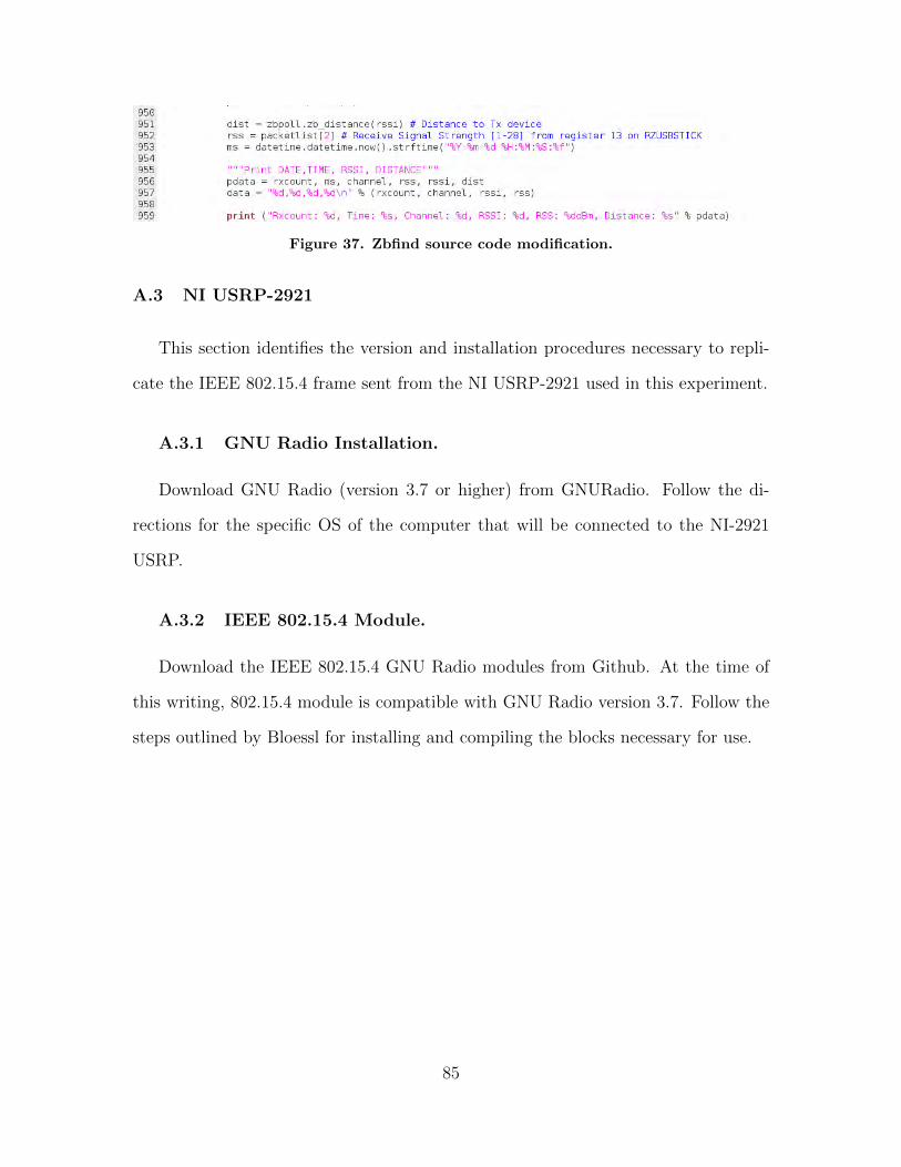
https://github.com/AFITWiSec/Z-Ranger

Figure 37. Zbfind source code modification.

A.3 NI USRP-2921

This section identifies the version and installation procedures necessary to repli-

cate the IEEE 802.15.4 frame sent from the NI USRP-2921 used in this experiment.

A.3.1 GNU Radio Installation.

Download GNU Radio (version 3.7 or higher) from GNURadio. Follow the di-

rections for the specific OS of the computer that will be connected to the NI-2921

USRP.

A.3.2 IEEE 802.15.4 Module.

Download the IEEE 802.15.4 GNU Radio modules from Github. At the time of

this writing, 802.15.4 module is compatible with GNU Radio version 3.7. Follow the

steps outlined by Bloessl for installing and compiling the blocks necessary for use.

85

http://gnuradio.org/redmine/projects/gnuradio/wiki

https://github.com/bastibl/gr-ieee802-15-4

Appendix B. Data Tables

B.1 RSSI-to-RSS Conversion Tables

B.1.1 Published MRF24J40 Converion Table.

Table 29. The MRF24J40 published RSS-to-RSSI values. Adapted from [Mic10].

RSS(dBm)

RSSI RSS(dBm)

RSSI RSS(dBm)

RSSI RSS(dBm)

RSSI

-100 0 -80 37 -60 138 -40 239-99 0 -79 43 -59 143 -39 245-98 0 -78 48 -58 148 -38 250-97 0 -77 53 -57 153 -37 253-96 0 -76 58 -56 159 -36 254-95 0 -75 63 -55 165 -35 255-94 0 -74 68 -54 170 -34 255-93 0 -73 73 -53 176 -33 255-92 0 -72 78 -52 183 -32 255-91 0 -71 83 -51 188 -31 255-90 0 -70 89 -50 193 -30 255-89 1 -69 95 -49 198 -29 255-88 2 -68 100 -48 203 -28 255-87 5 -67 107 -47 207 -27 255-86 9 -66 111 -46 212 -26 255-85 13 -65 117 -45 216 -25 255-84 18 -64 121 -44 221 -24 255-83 23 -63 125 -43 225 -23 255-82 27 -62 129 -42 228 -22 255-81 32 -61 133 -41 233 -21 255

-20 255

86

B.1.2 Extended MRF24J40 Conversion Table.

Table 30. Extended RSSI-to-RSS mapping for the Zena Wireless Adapter.

RSS

(dBm)

RSSI RSS

(dBm)

RSSI RSS

(dBm)

RSSI RSS

(dBm)

RSSI RSS

(dBm)

RSSI

-90 0 -77.4 51 -67.71 102 -57 153 -47.75 204-89 1 -77.2 52 -67.56 103 -56.83 154 -47.5 205-88 2 -77 53 -67.42 104 -56.66 155 -47.25 206-87.66 3 -76.8 54 -67.28 105 -56.5 156 -47 207-87.33 4 -76.6 55 -67.14 106 -56.33 157 -46.8 208-87 5 -76.4 56 -67 107 -56.17 158 -46.6 209-87.75 6 -76.2 57 -66.75 108 -56 159 -46.4 210-86.5 7 -76 58 -66.5 109 -55.83 160 -46.2 211-86.25 8 -75.8 59 -66.25 110 -55.66 161 -46 212-86 9 -75.6 60 -66 111 -55.5 162 -45.75 213-85.75 10 -75.4 61 -65.83 112 -55.33 163 -45.5 214-85.5 11 -75.2 62 -65.66 113 -55.17 164 -45.25 215-85.25 12 -75 63 -65.5 114 -55 165 -45 216-85 13 -74.8 64 -65.33 115 -54.8 166 -44.8 217-84.8 14 -74.6 65 -65.17 116 -54.6 167 -44.6 218-84.6 15 -74.4 66 -65 117 -54.4 168 -44.4 219-84.4 16 -74.2 67 -64.75 118 -54.2 169 -44.2 220-84.2 17 -74 68 -64.5 119 -54 170 -44 221-84 18 -73.8 69 -64.25 120 -53.83 171 -43.75 222-83.8 19 -73.6 70 -64 121 -53.66 172 -43.5 223-83.6 20 -73.4 71 -63.75 122 -53.5 173 -43.25 224-83.4 21 -73.2 72 -63.5 123 -53.33 174 -43 225-83.2 22 -73 73 -63.25 124 -53.17 175 -42.66 226-83 23 -72.8 74 -63 125 -53 176 -42.33 227-82.75 24 -72.6 75 -62.75 126 -52.86 177 -42 228-82.5 25 -72.4 76 -62.5 127 -52.71 178 -41.8 229-82.25 26 -72.2 77 -62.25 128 -52.56 179 -41.6 230-82 27 -72 78 -62 129 -52.42 180 -41.4 231-81.8 28 -71.8 79 -61.75 130 -52.28 181 -41.2 232-81.6 29 -71.6 80 -61.5 131 -52.14 182 -41 233-81.4 30 -71.4 81 -61.25 132 -52 183 -40.83 234-81.2 31 -71.2 82 -61 133 -51.8 184 -40.66 235-81 32 -71 83 -60.8 134 -51.6 185 -40.5 236-80.8 33 -70.83 84 -60.6 135 -51.4 186 -40.33 237-80.6 34 -70.66 85 -60.4 136 -51.2 187 -40.17 238-80.4 35 -70.5 86 -60.2 137 -51 188 -40 239-80.2 36 -70.33 87 -60 138 -50.8 189 -39.83 240-80 37 -70.17 88 -59.8 139 -50.6 190 -39.66 241-79.83 38 -70 89 -59.6 140 -50.4 191 -39.5 242-79.66 39 -69.83 90 -59.4 141 -50.2 192 -39.33 243-79.5 40 -69.66 91 -59.2 142 -50 193 -39.17 244

87

Table 30. Extended RSSI-to-RSS mapping for Zena wireless adapter.

Continuation of Table 5RSS

(dBm)

RSSI RSS

(dBm)

RSSI RSS

(dBm)

RSSI RSS

(dBm)

RSSI RSS

(dBm)

RSSI

-79.33 41 -69.5 92 -59 143 -49.8 194 -39 245-79.17 42 -69.33 93 -58.8 144 -49.6 195 -38.8 246-79 43 -69.17 94 -58.6 145 -49.4 196 -38.6 247-78.8 44 -69 95 -58.4 146 -49.2 197 -38.4 248-78.6 45 -68.8 96 -58.2 147 -49 198 -38.2 249-78.4 46 -68.6 97 -58 148 -48.8 199 -38 250-78.2 47 -68.4 98 -57.8 149 -48.6 200 -37.66 251-78 48 -68.2 99 -57.6 150 -48.4 201 -37.33 252-77.8 49 -68 100 -57.4 151 -48.2 202 -37 253-77.6 50 -67.86 101 -57.2 152 -48 203 -36 254

-35 255End of Table 5

88

B.2 Best fit Parameter Discovery Tables

B.2.1 Indoor Targets.

Table 31. Best fit values for P ∈ {1.6-4.0} for the Phillips Hue Bridge

Z-Ranger ZbfindP A (dBm) MAPE(%) A (dBm) MAPE(%)1.6 -51.0 68.780 -48.0 43.7801.7 -49.8 67.090 -46.6 39.5481.8 -48.6 65.322 -45.6 36.8101.9 -47.4 63.589 -44.3 35.9782.0 -46.1 61.758 -43.0 35.4602.1 -44.9 59.896 -41.7 35.0292.2 -43.6 58.019 -40.4 34.6752.3 -35.5 55.054 -39.1 34.4132.4 -35.1 51.809 -37.8 34.2142.5 -35.1 49.426 -36.5 34.0642.6 -35.1 47.618 -35.3 33.9352.7 -35.1 46.232 -33.9 33.8942.8 -35.1 45.161 -32.8 33.8742.9 -35.1 44.377 -32.0 34.1913.0 -33.8 43.758 -31.1 34.4643.1 -32.5 43.222 -30.1 34.8423.2 -30.0 42.704 -28.7 35.3683.3 -29.4 42.221 -27.8 36.1493.4 -28.9 41.820 -27.4 37.0183.5 -27.7 41.128 -26.9 37.8013.6 -26.5 42.476 -26.1 38.7443.7 -26.3 42.844 -25.2 39.6283.8 -26.5 43.177 -24.4 40.4863.9 -25.4 43.522 -23.6 41.3014.0 -24.2 43.882 -22.7 42.333

89

Table 32. Best fit values for P ∈ {1.6-4.0} for the Awarepoint S2


90

Table 33. Best fit values for P ∈ {1.6-4.0} for the Freescale MC13213

Z-Ranger ZbfindP A (dBm) MAPE(%) A (dBm) MAPE(%)1.6 -50.3 46.133 -53.1 43.0141.7 -49.0 42.939 51.3 40.3491.8 -46.1 39.005 50.3 38.8171.9 -46.0 36.221 -48.8 38.3552.0 -45.2 34.781 -47.8 37.9662.1 -43.9 33.890 -46.8 37.8842.2 -42.6 33.091 -45.9 38.0462.3 -41.4 32.368 -44.7 38.6872.4 -40.1 31.711 -43.7 39.4642.5 -38.8 31.153 -42.6 40.2272.6 -38.0 31.134 -41.7 40.9952.7 -37.5 31.505 -40.6 41.7292.8 -36.1 32.128 -39.7 42.4652.9 -35.2 33.159 -39.9 43.1433.0 -34.4 34.296 -39.1 43.7563.1 -33.7 35.367 -38.2 44.3573.2 -33.1 36.354 -37.7 45.1693.3 -31.9 37.538 -36.6 46.1213.4 -30.8 38.745 -35.7 47.4763.5 -29.6 39.931 -34.9 48.7473.6 -28.4 41.109 -34.0 49.9713.7 -27.3 42.281 -33.2 51.0923.8 -28.8 43.345 -32.4 52.1863.9 -28.1 44.275 -31.5 52.2074.0 -27.3 45.165 -30.7 54.182

91

Table 34. Best fit values for P ∈ {1.6-4.0} for the Atmel RZUSBstick

Z-Ranger ZbfindP A (dBm) MAPE(%) A (dBm) MAPE(%)1.6 -53.6 55.025 -65.3 44.6931.7 -53.1 51.609 -62.6 41.1391.8 -52.6 48.899 61.2 37.1411.9 -52.0 46.719 -61.0 34.5212.0 -50.7 47.390 -59.6 33.4132.1 -49.6 46.174 -58.7 33.0012.2 -49.6 46.262 -58.2 33.1142.3 -49.6 46.357 -57.2 33.5472.4 -49.6 46.452 -56.0 34.0372.5 -49.6 46.669 -54.8 34.5882.6 -48.4 47.059 -53.4 35.2932.7 -47.4 47.519 -52.1 36.0272.8 -46.4 48.026 -50.7 36.7952.9 -45.3 48.517 -49.3 37.5913.0 -44.3 49.022 -47.9 38.4133.1 -43.2 49.553 -46.5 39.2553.2 -42.2 50.055 -45.1 40.1163.3 -41.2 50.596 -43.7 40.9903.4 -40.1 51.119 -42.3 41.8773.5 -39.1 51.644 -40.9 42.7733.6 -38.4 52.280 -41.4 43.5823.7 -37.7 52.886 -40.2 44.3783.8 -37.0 53.462 -38.9 45.1663.9 -36.3 54.013 -37.7 45.9384.0 -35.6 54.539 -36.5 46.699

92

B.2.2 Outdoor Targets.

Table 35. Best fit values for P ∈ {1.6-4.0} for the Openway CENTRON smart meter


93

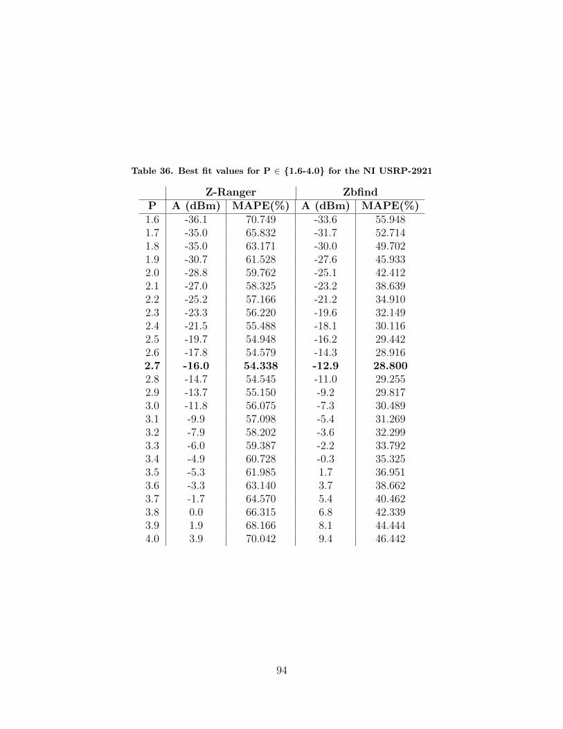
Table 36. Best fit values for P ∈ {1.6-4.0} for the NI USRP-2921

Z-Ranger ZbfindP A (dBm) MAPE(%) A (dBm) MAPE(%)1.6 -36.1 70.749 -33.6 55.9481.7 -35.0 65.832 -31.7 52.7141.8 -35.0 63.171 -30.0 49.7021.9 -30.7 61.528 -27.6 45.9332.0 -28.8 59.762 -25.1 42.4122.1 -27.0 58.325 -23.2 38.6392.2 -25.2 57.166 -21.2 34.9102.3 -23.3 56.220 -19.6 32.1492.4 -21.5 55.488 -18.1 30.1162.5 -19.7 54.948 -16.2 29.4422.6 -17.8 54.579 -14.3 28.9162.7 -16.0 54.338 -12.9 28.8002.8 -14.7 54.545 -11.0 29.2552.9 -13.7 55.150 -9.2 29.8173.0 -11.8 56.075 -7.3 30.4893.1 -9.9 57.098 -5.4 31.2693.2 -7.9 58.202 -3.6 32.2993.3 -6.0 59.387 -2.2 33.7923.4 -4.9 60.728 -0.3 35.3253.5 -5.3 61.985 1.7 36.9513.6 -3.3 63.140 3.7 38.6623.7 -1.7 64.570 5.4 40.4623.8 0.0 66.315 6.8 42.3393.9 1.9 68.166 8.1 44.4444.0 3.9 70.042 9.4 46.442

94

Appendix C. Windowing Table Results

C.1 Z-Ranger

C.1.1 Indoor RSS Sliding Window.

C.1.1.1 Z-Ranger.

Table 37. Indoor RSS sliding window MAPE comparison for Z-Ranger.

Method Hue S2 MC13213 RZUSBstick MAPE ImprovementBest fit 51.86% 31.67% 36.06% 58.64% 44.56% -

2-Window 51.97% 26.29% 33.10% 59.39% 42.69% 4.2%3-Window 52.03% 26.98% 33.09% 59.36% 42.87% 3.8%

C.1.1.2 Zbfind.

Table 38. Indoor RSS sliding window MAPE comparison for Zbfind.


2-Window 64.45% 85.26% 49.03% 89.25% 72.00% -5.2%3-Window 64.62% 84.71% 48.95% 88.56% 71.71% -4.8%

C.1.2 Outdoor RSS Sliding Window.

C.1.2.1 Z-Ranger.

Table 39. Outdoor RSS sliding window MAPE comparison for Z-Ranger.

Method CENTRON NI USRP-2921 MAPE ImprovementBest fit 80.93% 62.78% 71.86% -

2-Window 102.78% 71.67% 87.23% -21.4%3-Window 99.06% 71.80% 85.43% -18.9%

C.1.2.2 Zbfind.

Table 40. Outdoor RSS sliding window MAPE comparison for Zbfind.


2-Window 220.18% 76.79% 148.49% -13.5%3-Window 220.12% 76.87% 148.50% -13.5%

95

C.1.3 Indoor RSS Sequential Window.

C.1.3.1 Z-Ranger.

Table 41. Indoor RSS sequential window MAPE comparison for Z-Ranger.


2-Window 52.02% 26.47% 35.84% 58.97% 43.33% 2.8%3-Window 51.91% 26.90% 35.96% 58.52% 43.33% 2.8%

C.1.3.2 Zbfind.

Table 42. Indoor RSS sequential window MAPE comparison for Zbfind.


2-Window 64.30% 84.82% 48.85% 88.66% 71.66% -4.8%3-Window 64.55% 82.63% 48.97% 87.29% 70.86% -3.6%

C.1.4 Outdoor RSS Sequential Window.

C.1.4.1 Z-Ranger.

Table 43. Outdoor RSS sequential window MAPE comparison for Z-Ranger.


2-Window 101.18% 71.67% 86.69% -20.6%3-Window 99.54% 71.91% 85.73% -19.3%

C.1.4.2 Zbfind.

Table 44. Outdoor RSS sequential window MAPE comparison for Zbfind.


2-Window 220.81% 76.74% 148.78% -13.7%3-Window 219.74% 76.79% 148.27% -13.3%

96

Bibliography

Ada06. J. Adams. An Introduction to IEEE STD 802.15.4. In 2006 IEEEAerospace Conference, page 8, 2006.

Atm09a. Atmel. Atmel AT86RF230 Data Sheet. http://www.atmel.com/images/doc5131.pdf [Accessed: 26 May 2015], February 2009.

Atm09b. Atmel. AVR2009: AT86RF230 Software Programming Model. Technicalreport, 2009.

Atm12. Atmel. Atmel AVR2016: RZRAVEN Hardware Users Guide. http://

www.atmel.com/Images/doc8117.pdf [Accessed: 5 January 2016], 2012.

Bio03. P. Biondi. The Scapy Project. http://www.secdev.org/projects/

scapy/ [Accessed: 21 October 2015], 2003.

Blo12. B. Bloessl. IEEE 802.15.4 ZigBee Transceiver. https://github.com/

bastibl/gr-ieee802-15-4/tree/master/apps [Accessed: 23 November2015], 2012.

BPC+07. P. Baronti, P. Pillai, V. Chook, S. Chessa, A. Gotta, and Y. Fun Hu.Wireless Sensor Networks: A Survey on the State of the Art and the802.15.4 and ZigBee Standards. In Computer Communications, volume 30,pages 1655–1695. Elsevier, 26 May 2007.

CR12. A. Coluccia and F. Ricciato. A Software-Defined Radio Tool for Experi-menting with RSS Measurements in IEEE 802.15.4: Implementation andApplications. In 2012 21st International Conference on Computer Com-munications and Networks (ICCCN), pages 1–6, 2012.

Des11. J. Desbonnet. Using the Microchip ZENA ZigBee/802.15.4 Net-work Analyzer with Linux. http://jdesbonnet.blogspot.com/2011/

02/using-microchip-zena-zigbee802154.html [Accessed: 27 August2015], 2011.

EPR10. EPRI. An Investigation of Radiofrequency Fields Associated with theItron Smart Meter. http://smartgridcc.org/wp-content/uploads/

2012/08/000000000001021126.pdf [Accessed: 11 November 2015], 2010.

Fre09. Freescale. MC13211/212/213 ZigBee- Compliant Platform - 2.4 GHzLow Power Transceiver for the IEEE 802.15.4 Standard plus Microcon-troller. https://cache.freescale.com/files/rf_if/doc/data_sheet/MC1321x.pdf?pspll=1 [Accessed: 11 November 2015], 2009.

97

http://www.atmel.com/images/doc5131.pdf

http://www.atmel.com/images/doc5131.pdf

http://www.atmel.com/Images/doc8117.pdf

http://www.atmel.com/Images/doc8117.pdf

http://www.secdev.org/projects/scapy/

http://www.secdev.org/projects/scapy/

https://github.com/bastibl/gr-ieee802-15-4/tree/master/apps

https://github.com/bastibl/gr-ieee802-15-4/tree/master/apps

http://jdesbonnet.blogspot.com/2011/02/using-microchip-zena-zigbee802154.html

http://jdesbonnet.blogspot.com/2011/02/using-microchip-zena-zigbee802154.html

http://smartgridcc.org/wp-content/uploads/2012/08/000000000001021126.pdf

http://smartgridcc.org/wp-content/uploads/2012/08/000000000001021126.pdf

https://cache.freescale.com/files/rf_if/doc/data_sheet/MC1321x.pdf?pspll=1

https://cache.freescale.com/files/rf_if/doc/data_sheet/MC1321x.pdf?pspll=1

GBM+12. T. Goodspeed, S. Bratus, R. Melgares, R. Speers, and S. Smith. Api-do:Tools for Exploring the Wireless Attack Surface in Smart Meters. In45th Hawaii International Conference on System Science (HICSS), pages2133–2140, 2012.

GGH10. S. Gansemer, U. Grossmann, and S. Hakobyan. RSSI-based EuclideanDistance Algorithm for Indoor Positioning Adapted for the use in Dynam-ically Changing WLAN Environments and Multi-level Buildings. In Inter-national Conference on Indoor Positioning and Indoor Navigation (IPIN),pages 1–6, 2010.

Goo09. T. Goodspeed. Extracting Keys from Second Generation ZigBee Chips.In Chipcon, Black Hat USA, 2009.

IEE03. IEEE. Standard for Local and Metropolitan Area Networks Part 15.4:Low-Rate Wireless Personal Area Networks (LR-WPANs), 2003.

IEE11. IEEE. Standard for Local and Metropolitan Area Networks Part 15.4:Low-Rate Wireless Personal Area Networks (LR-WPANs), 2011.

IEE15. IEEE. IEEE About Page. http://www.ieee.org/about/ieee_history.html [Accessed: 21 October 2015], 2015.

Jih11. C. Jihong. Patient Positioning System in Hospital Based on Zigbee. InInternational Conference on Intelligent Computation and Bio-Medical In-strumentation (ICBMI), pages 159–162, 2011.

JL09. Z. Jianwu and Z. Lu. Research on Distance Measurement Based on RSSIof ZigBee. In ISECS International Colloquium on Computing, Commu-nication, Control, and Management (CCCM), volume 3, pages 210–212,August 2009.

Koh95. R. Kohavi. A Study of Cross-Validation and Bootstrap for Accuracy Es-timation and Model Selection. In International Joint Conference on Arti-ficial Intelligence (IJCAI), 1995.

Mic10. Microchip. MRF24J40 Data Sheet: IEEE 802.15.4 2.4 GHz RFTransceiver. http://ww1.microchip.com/downloads/en/DeviceDoc/

39776C.pdf [Accessed: 6 January 2016], 2010.

Mic11. Microchip. Zena Wireless Adapter. https://www.microchip.com/

DevelopmentTools/ProductDetails.aspx?PartNO=AC182015-1 [Ac-cessed: 21 August 2015], 2011.

Mic12. Microchip. Wireless Development Studio. https://www.microchip.com/stellent/idcplg?IdcService=SS_GET_PAGE&nodeId=2680&dDocName=

en554472 [Accessed: 9 August 2015], 2012.

98

http://www.ieee.org/about/ieee_history.html

http://www.ieee.org/about/ieee_history.html

http://ww1.microchip.com/downloads/en/DeviceDoc/39776C.pdf

http://ww1.microchip.com/downloads/en/DeviceDoc/39776C.pdf

https://www.microchip.com/DevelopmentTools/ProductDetails.aspx?PartNO=AC182015-1

https://www.microchip.com/DevelopmentTools/ProductDetails.aspx?PartNO=AC182015-1

https://www.microchip.com/stellent/idcplg?IdcService=SS_GET_PAGE&nodeId=2680&dDocName=en554472



Mic16. Microsoft. USB Endpoints and their Pipes. https://msdn.microsoft.

com/en-us/library/windows/hardware/dn303353(v=vs.85).aspx [Ac-cessed: 26 January 2016], 2016.

MSB11. R. Melgares, R. Speers, and S. Bratus. Api-do: Tools for Zig-Bee and 802.15.4 Security Auditing. https://code.google.com/p/

zigbee-security/ [Accessed: 20 October 2015], 2011.

Osc15. Oscium. WiPry Pro. https://www.oscium.com/spectrum-analyzers/

wipry-pro-combo [Accessed: 12 November 2015), 2015.

Poo15. I. Poole. Radio Signal Path Loss. http://www.radio-electronics.

com/info/propagation/path-loss/rf-signal-loss-tutorial.php

[Accessed: 9 November 2015], 2015.

Rad15. GNU Radio. GNU Radio: The Free and Open Software Radio Ecosys-tem. https://gnuradio.org/redmine/projects/gnuradio [Accessed:11 November 2015], 2015.

Ran15. Random. Random Team Generator. http://www.randomlists.com/

team-generator[Accessed: 20 November 2015], 2015.

Rap96. T. Rappaport. Wireless Communication Principles and Practice, chap-ter 3, page 102. 1996.

RMLS14. B. Ramsey, B. Mullins, W. Lowder, and R. Speers. Sharpening the Stinger:Tuning KillerBee for Critical Infrastructure Warwalking. In IEEE MilitaryCommunications Conference (MILCOM), pages 104–109, 2014.

RMW12. B. Ramsey, B. Mullins, and E. White. Improved Tools for Indoor ZigBeeWarwalking. In 7th IEEE International Workshop on Practical Issues inBuilding Sensor Network Applications, 2012.

ROA12. M. Raju, T. Oliveira, and D. Agrawal. A Practical Distance Estima-tor Through Distributed RSSI/LQI Processing-An Experimental Study.In IEEE International Conference on Communications (ICC), pages6575–6579, 2012.

Sch06. T. Schmid. GNU Radio 802.15.4 En- and Decoding. http:

//citeseerx.ist.psu.edu/viewdoc/download?doi=10.1.1.179.

31&rep=rep1&type=pdf [Accessed: 23 Nov 2015], 2006.

Sec15. Offensive Security. Kali Linux 2.0. https://www.kali.org/[Accessed: 22October 2015], 2015.

Sei16. A. Seitz. Z-Ranger. https://github.com/AFITWiSec/Z-Ranger [Ac-cessed: 23 January 2016], 2016.

99

https://msdn.microsoft.com/en-us/library/windows/hardware/dn303353(v=vs.85).aspx

https://msdn.microsoft.com/en-us/library/windows/hardware/dn303353(v=vs.85).aspx

https://code.google.com/p/zigbee-security/

https://code.google.com/p/zigbee-security/

https://www.oscium.com/spectrum-analyzers/wipry-pro-combo

https://www.oscium.com/spectrum-analyzers/wipry-pro-combo

http://www.radio-electronics.com/info/propagation/path-loss/rf-signal-loss-tutorial.php

http://www.radio-electronics.com/info/propagation/path-loss/rf-signal-loss-tutorial.php

https://gnuradio.org/redmine/projects/gnuradio

http://www.randomlists.com/team-generator

http://www.randomlists.com/team-generator

http://citeseerx.ist.psu.edu/viewdoc/download?doi=10.1.1.179.31&rep=rep1&type=pdf



https://www.kali.org/

https://github.com/AFITWiSec/Z-Ranger

SKG12. F. Schuster, W. Kastner, and W. Granzer. Integrating Smart Cameras intoZigBee. In 9th IEEE International Workshop on Factory CommunicationSystems (WFCS), pages 67–70, 2012.

SRMR16. A. Seitz, B. Ramsey, B. Mullins, and M. Rice. Z-Ranger: An ImprovedTool Set for ZigBee Warwalking. In International Conference on CyberWarfare and Security (ICCWS), 2016.

Ver13. E. Verschuur. ZenaNG Linux. https://github.com/emericv/ZenaNG

[Accessed: 21 October 2015], 2013.

Whi07. T. Whittaker. Final Word. In Control and Automation, volume 18,page 48. 2007.

WSM10. J. Wright, R. Speers, and R. Melgares. KillerBee: Framework and Toolsfor Exploiting ZigBee and IEEE 802.15.4 Networks. https://github.

com/riverloopsec/killerbee [Accessed: 15 October 2015], 2010.

XC11. Y. Xu and X. Chen. Node Localization in Wireless Sensor Network UsingDynamic Distance Prediction Algorithm. In IEEE Instrumentation andMeasurement Technology Conference (I2MTC), pages 1–4, 2011.

Zig12. ZigBee. ZigBee Specification. www.zigbee.org/ [Accessed: 15 March2015], 2012.

Zig15. ZigBee. ZigBee Alliance. http://www.zigbee.org/zigbeealliance/

[Accessed: 20 October 2015], 2015.

100

https://github.com/emericv/ZenaNG

https://github.com/riverloopsec/killerbee

https://github.com/riverloopsec/killerbee

www.zigbee.org/

http://www.zigbee.org/zigbeealliance/

REPORT DOCUMENTATION PAGE Form ApprovedOMB No. 0704–0188

The public reporting burden for this collection of information is estimated to average 1 hour per response, including the time for reviewing instructions, searching existing data sources, gathering andmaintaining the data needed, and completing and reviewing the collection of information. Send comments regarding this burden estimate or any other aspect of this collection of information, includingsuggestions for reducing this burden to Department of Defense, Washington Headquarters Services, Directorate for Information Operations and Reports (0704–0188), 1215 Jefferson Davis Highway,Suite 1204, Arlington, VA 22202–4302. Respondents should be aware that notwithstanding any other provision of law, no person shall be subject to any penalty for failing to comply with a collectionof information if it does not display a currently valid OMB control number. PLEASE DO NOT RETURN YOUR FORM TO THE ABOVE ADDRESS.

1. REPORT DATE (DD–MM–YYYY) 2. REPORT TYPE 3. DATES COVERED (From — To)

4. TITLE AND SUBTITLE 5a. CONTRACT NUMBER

5b. GRANT NUMBER

5c. PROGRAM ELEMENT NUMBER

5d. PROJECT NUMBER

5e. TASK NUMBER

5f. WORK UNIT NUMBER

6. AUTHOR(S)

7. PERFORMING ORGANIZATION NAME(S) AND ADDRESS(ES) 8. PERFORMING ORGANIZATION REPORTNUMBER

9. SPONSORING / MONITORING AGENCY NAME(S) AND ADDRESS(ES) 10. SPONSOR/MONITOR’S ACRONYM(S)

11. SPONSOR/MONITOR’S REPORTNUMBER(S)

12. DISTRIBUTION / AVAILABILITY STATEMENT

13. SUPPLEMENTARY NOTES

14. ABSTRACT

15. SUBJECT TERMS

16. SECURITY CLASSIFICATION OF:

a. REPORT b. ABSTRACT c. THIS PAGE

17. LIMITATION OFABSTRACT

18. NUMBEROFPAGES

19a. NAME OF RESPONSIBLE PERSON

19b. TELEPHONE NUMBER (include area code)

Standard Form 298 (Rev. 8–98)Prescribed by ANSI Std. Z39.18

24–03–2016 Master’s Thesis May 2014 — Mar 2016

A Comparative Analysis of IEEE 802.15.4 Adapters for WirelessRangefinding

JON 16G129

Seitz, Andrew P., MSgt, USAF

Air Force Institute of TechnologyGraduate School of Engineering and Management (AFIT/EN)2950 Hobson WayWPAFB OH 45433-7765


AFRL Information DirectoratePOC: Hiren Patel, Cyber ISR Program ManagerATTN: Hiren Patel AFRL/RIGDMailstop: 525 Brooks Rd, Rome, NY, 13441Email: [email protected] Phone: 315-330-4315 AFRL/RIGD


This work is declared a work of the U.S. Government and is not subject to copyright protection in the United States.

ZigBee offers low-cost mesh connectivity in hospitals, refineries, and critical infrastructure. This thesis explores twoZigBee Received Signal Strength Indicator (RSSI)-based rangefinding tool sets: Z-Ranger and Zbfind. Z-Ranger is a newtool set developed herein for the Zena Wireless Adapter that offers configurable distance estimating parameters and aRSSI resolution of 256 values. Zbfind is an application developed for the Atmel RZUSBstick with no configurabledistance estimating parameters and a RSSI resolution of 29 values. The two tool sets are evaluated while rangefindingfour wireless devices indoors and two devices outdoors. Mean error is calculated at each of the 35 collection points and a99% confidence interval and p− Test are used to identify statistical deviations between the two. After three rounds ofevaluation, the results suggest that calibrated distance estimating parameters along with an increased RSSI resolution donot statistically reduce mean error when compared to non-calibrated parameters and lower RSSI resolution. The result ofthis research is that Z-Ranger is shown to be an alternative rangefinding tool set that performs as well as Zbfind.

ZigBee, Warwalking, RSSI-based Distance Estimation, Low-rate sensor

U U U U 121

Dr. Benjamin Ramsey, AFIT/ENG

(937) 255-3636x4603; [email protected]

air force institute of technology - dtic.mil · 22 the ni usrp-2921 is positioned at the 0 m marker...

Documents