air quality assessment of the pengrowth lindbergh … files/volume ii/consultant...pengrowth energy...
TRANSCRIPT

Suite 217, 811 - 14 Street N.W. Calgary, AB Canada T2N 2A4 Tel: 403 592-6180 Fax: 403 283-2647 Email: [email protected] / www.mems.ca
Air Quality Assessment of the Pengrowth Lindbergh SAGD Project
Prepared for: Pengrowth Energy Corporation
Prepared by: Millennium EMS Solutions Ltd. Suite 217, 811 – 14th Street NW
Calgary, Alberta T2N 2A4
December 2011 File # 11-032

Pengrowth Energy Corporation Air Quality Assessment of the Lindbergh SAGD Project Millennium EMS Solutions Ltd. December 2011
Page i 11-032
Executive Summary
Pengrowth Energy Corporation (Pengrowth) is proposing to develop a 12,500 barrel (1,987 m3) per day (bpd) Steam Assisted Gravity Drainage (SAGD) Project on their Lindbergh lease (Oil Sands Leases #0727288080033, 072728808A033 and 0757598120181). The Lindbergh SAGD Project is located approximately 22 km southeast of Bonnyville and approximately 19 km east along Highway 646 from the Town of Elk Point, in the County of St. Paul. Millennium EMS Solutions Ltd. (MEMS) was retained to provide an air quality assessment of typical facility operations of NOx, SO2, CO and PM2.5 emissions. The modelling assessment was done in accordance with Alberta Environment and Water’s (AEW) requirements for EPEA Amendment applications and follows the most recent AEW modelling guidance (AEW, 2009).
Operations at the plant will result in emissions to the atmosphere. These emissions include combustion products such as sulphur dioxide (SO2), carbon monoxide (CO), oxides of nitrogen (NOx),
and particulate matter less than 2.5 m in diameter (PM2.5). These contaminants may be harmful to
human health at sufficiently high ambient ground-level concentrations and as such, should not exceed Alberta ambient air quality objectives (AAAQO).
The results of dispersion modelling showed there were no predicted exceedances for SO2, NOx, PM2.5
or CO for any averaging period. An upset flaring assessment was also performed and results showed no predicted exceedances of hourly SO2 or NO2 AAAQOs.

Pengrowth Energy Corporation Air Quality Assessment of the Lindbergh SAGD Project Millennium EMS Solutions Ltd. December 2011
Page ii 11-032
Table of Contents Page
Executive Summary ................................................................................................................................. i
Table of Contents ................................................................................................................................... ii
List of Tables ......................................................................................................................................... iii
List of Figures ........................................................................................................................................ iii
List of Appendices ................................................................................................................................. iv
1.0 INTRODUCTION ........................................................................................................................ 1
2.0 AIR QUALITY CRITERIA ........................................................................................................... 1
2.1 Ambient Air Quality Objectives ............................................................................................... 1
2.2 Relationship Between NOx and NO2 ....................................................................................... 2
3.0 EMISSION PARAMETERS ........................................................................................................ 3
3.1 Project Emissions ................................................................................................................... 3
3.2 Regional Emissions ................................................................................................................ 9
4.0 DISPERSION MODELLING APPROACH ................................................................................ 13
4.1 Model Parameters ................................................................................................................. 13
4.2 Meteorological Data .............................................................................................................. 13
4.3 Background Concentrations .................................................................................................. 16
5.0 DISPERSION MODEL PREDICTIONS .................................................................................... 16
5.1 Sulphur Dioxide Model Predictions ....................................................................................... 17
5.2 Nitrogen Dioxide Model Predictions ...................................................................................... 22
5.3 PM2.5 Model Predictions ........................................................................................................ 25
5.4 CO Model Predictions ........................................................................................................... 27
6.0 UPSET MODELLING ............................................................................................................... 30
7.0 SUMMARY AND CONCLUSIONS ........................................................................................... 33
8.0 CLOSURE ................................................................................................................................ 33
9.0 REFERENCES ......................................................................................................................... 34

Pengrowth Energy Corporation Air Quality Assessment of the Lindbergh SAGD Project Millennium EMS Solutions Ltd. December 2011
Page iii 11-032
List of Tables Page
Table 2.1 Alberta Ambient Air Quality Objectives and Canada Wide Standards ............................ 1
Table 2.2 Background Ozone (from Cold Lake South Monitoring Station) used for NO2 Conversion ...................................................................................................................... 3
Table 3.1 Pengrowth Lindbergh Stack Emission Sources .............................................................. 4
Table 3.2 CCME Emission and Performance Target Compliance for Boilers and Heaters ............ 5
Table 3.3 CPF Building Dimensions ............................................................................................... 6
Table 3.4 CPF Storage Tank Dimensions ....................................................................................... 7
Table 3.5 Summary of Existing & Approved Regional Emissions ................................................. 11
Table 3.6 Summary of Planned Regional Emissions .................................................................... 12
Table 4.1 Ambient Background Concentrations of Modelled Compounds .................................... 16
Table 5.1 Summary of Predicted SO2 Maximum Ground-Level Concentrations (g/m3) ............. 17
Table 5.2 Summary of NO2 Maximum Predicted Ground-Level Concentrations (μg/m3) .............. 22
Table 5.3 Summary of PM2.5 Maximum Ground-Level Concentrations (μg/m3) ............................ 25
Table 5.4 Summary of CO Maximum Ground-Level Concentrations (μg/m3) ............................... 27
Table 6.1 Emergency Generator Parameters and Emissions ....................................................... 30
Table 6.2 Flare Stack and Emission Parameters .......................................................................... 31
Table 6.3 Predicted 9th Highest Hourly Concentration from Emergency Generator Operation – Upset Case #1 (including Project and Regional Sources) (g/m3)............................. 32
Table 6.4 Predicted Hourly Concentration from Upset Flaring (including Project and Regional Sources) (g/m3) ........................................................................................................... 32
List of Figures Page
Figure 3.1 Buildings, Structures and Tanks Considered for Downwash Effects .............................. 8
Figure 3.2 Regional Facilities Included in Modelling ...................................................................... 10
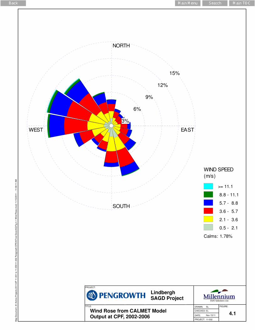
Figure 4.1 Wind Rose from CALMET Model Output at the CPF, 2002-2006 ................................. 15
Figure 5.1 Predicted 99.9th Percentile Hourly SO2 Concentrations (µg/m3) .................................... 18
Figure 5.2 Predicted 2nd Highest 24-hour SO2 Concentrations (µg/m3) ......................................... 19
Figure 5.3 Predicted Maximum Monthly SO2 Concentrations (µg/m3) ............................................ 20
Figure 5.4 Predicted Annual Average SO2 Concentrations (µg/m3) ............................................... 21
Figure 5.5 Predicted 99.9th Percentile Hourly NO2 Concentrations (µg/m3) ................................... 23
Figure 5.6 Predicted Annual Average NO2 Concentrations (µg/m3) ............................................... 24
Figure 5.7 Predicted 2nd Highest 24-hour PM2.5 Concentrations (µg/m3) ....................................... 26
Figure 5.8 Predicted 99.9th Percentile Hourly CO Concentrations (µg/m3) .................................... 28
Figure 5.9 Predicted Maximum 8-Hour CO Concentrations (µg/m3) .............................................. 29

Pengrowth Energy Corporation Air Quality Assessment of the Lindbergh SAGD Project Millennium EMS Solutions Ltd. December 2011
Page iv 11-032
List of Appendices
Appendix A Modelling Parameters
Appendix B CCME Emission Rate Sample Calculation

Pengrowth Energy Corporation Air Quality Assessment of the Lindbergh SAGD Project Millennium EMS Solutions Ltd. December 2011
Page 1 11-032
1.0 INTRODUCTION
Pengrowth Energy Corporation (Pengrowth) is proposing to develop a 12,500 barrel (1,987 m3) per day (bpd) Steam Assisted Gravity Drainage (SAGD) Project on their Lindbergh lease (Oil Sands Leases #0727288080033, 072728808A033 and 0757598120181). The Lindbergh SAGD Project is located approximately 22 km southeast of Bonnyville and approximately 22 km east along Highway 646 from the Town of Elk Point, in the County of St. Paul. The Lindbergh leases are located within Townships 58-59, Ranges 4-5, west of the 4th Meridian. The proposed Lindbergh SAGD Project will be located in Sections 13, 14, 23, 24, 25 and 26, Twp 58, Rge 5, west of the 4th Meridian. Pengrowth is currently developing the 200 m3/d Lindbergh SAGD Pilot Project which is located in Section 13, Twp 58, Rge 5, west of the 4th Meridian. Millennium EMS Solutions Ltd. (MEMS) was retained to provide an air quality assessment of typical facility operations of NOx, SO2, CO and PM2.5 emissions.
Building downwash effects were considered in the Lindbergh modelling. All buildings and structures within the areas of influence for downwash were included in the downwash model.
All emissions from industrial facilities operating within a 40 x 40 km area centered on the Pengrowth Lindbergh facility were explicitly modelled.
The modelling was executed following the latest AEW (2009) dispersion modelling guidance. The CALMET model, including 5 years (2002-2006) of meteorological data, was used in this modelling. This report outlines the assumptions, the dispersion modelling approach, model input data, and the dispersion modelling results.
2.0 AIR QUALITY CRITERIA
2.1 Ambient Air Quality Objectives
The Alberta Ambient Air Quality objectives (AAAQOs) for Project emissions are presented in Table 2.1. The objectives refer to averaging periods ranging from one hour to one year.
Table 2.1 Alberta Ambient Air Quality Objectives and Canada Wide Standards
Parameter Period Alberta Objectives(a)
Canada Wide Standards(b)
[µg/m3] [µg/m3]
SO2
Annual 20 –
30-day 30 –
24-hour 125 –
1-hour 450 –
NO2 Annual 45 –
1-hour 300 –

Pengrowth Energy Corporation Air Quality Assessment of the Lindbergh SAGD Project Millennium EMS Solutions Ltd. December 2011
Page 2 11-032
Table 2.1 Alberta Ambient Air Quality Objectives and Canada Wide Standards
Parameter Period Alberta Objectives(a)
Canada Wide Standards(b)
[µg/m3] [µg/m3]
CO 8-hour 6,000 –
1-hour 15,000 –
PM2.5 24-hour 30 30(c)
1-hour 80(d) -– (a) Source: AEW (2011) (b) Source: CCME (2000) (c) 98th percentile (d) Alberta Ambient Air Quality Guideline (AAAQG) - No air quality standard or guideline for this averaging period/parameter
2.2 Relationship Between NOx and NO2
Oxides of nitrogen (NOx) are comprised of nitric oxide (NO) and nitrogen dioxide (NO2). High temperature combustion processes primarily produce NO that in turn can be converted to NO2 in the atmosphere through reactions with tropospheric ozone:
NO + O3 → NO2 + O2
Conversion of NOx to NO2 is estimated using the AEW (2009) recommended Ozone Limiting Method (OLM), which has been established through the consideration of lowest observable effect level on a sensitive receptor. This method states that if the ambient ozone concentration is greater than 90% of the predicted NOx, then it is assumed that all the NOx is converted to NO2. Otherwise, the NO2 concentration is equal to the sum of the ozone and 10% of the predicted NOx concentration. That is:
If [O3] > 0.9 [NOx], then [NO2] = [NOx]
Otherwise, [NO2] = [O3] + 0.1 [NOx]
The 95th percentile of the observed O3 ambient concentrations from the Cold Lake South air quality monitoring station were used in the NO2 conversion calculations (Table 2.2). AEW requires that if the OLM method is used, NO2 concentration results assuming total conversion of NOx to NO2 also be presented.
Pengrowth Energy Corporation Air Quality Assessment of the Lindbergh SAGD Project Millennium EMS Solutions Ltd. December 2011
Page 3 11-032
Table 2.2 Background Ozone (from Cold Lake South Monitoring Station) used for NO2 Conversion
Averaging Period Observed Concentration (g/m3) Data Type
1 hour 96 95th Percentile
Annual 50 Average
Data Source: CASA Data Warehouse (2011)
3.0 EMISSION PARAMETERS
3.1 Project Emissions
Under typical facility operation there will be emissions from four continuous sources and two intermittent sources. Continuous emissions are from three steam boilers and one co-generation unit. A utility boiler and a glycol heater are both run intermittently and/or seasonally, but are modeled conservatively as continuous sources. Modelled stack and emission parameters are presented in Table 3.1.
All equipment duties were based on preliminary engineering and design. All emissions were provided by Pengrowth. SO2 emissions were estimated from AP-42 emission factors (US EPA 1998) plus SO2 produced through the combustion of H2S from the reservoir. NOx, CO and PM2.5 emissions were estimated from AP-42 emission factors. NOx and CO emissions for the boilers and heaters were designed to meet the CCME guidelines for Commercial/Industrial Boilers and Heaters (CCME, 1998), as presented in Table 3.2. A sample emission intensity calculation is presented in Appendix B.
A natural gas-fired emergency generator unit will provide back-up power, as required. In addition, two upset flaring scenarios were evaluated. Emissions and results from these three upset cases are presented in Section 6.
The generation of downwash by buildings located within the facility compound was considered. Figure 3.1 shows the Pengrowth Lindbergh property line, buildings and structures considered for downwash generation, and all stack emission sources modelled. Downwash was considered for Project emissions only. Tables 3.3 and 3.4 list the buildings and tanks, respectively, considered in the model and their respective dimensions.

Pengrowth Energy Corporation Air Quality Assessment of the Lindbergh SAGD Project Millennium EMS Solutions Ltd. December 2011
Page 4 11-032
Table 3.1 Pengrowth Lindbergh Stack Emission Sources
Source Description
Input Power Rating (kW)
UTM Coordinates (m) Elevation
(m ASL)
StackHeight
(m)
Stack Diameter
(m)
Exit Velocity
(m/s)
Exit Temp.
(K)
Emissions (t/d)
Easting Northing SO2 NOx CO PM2.5
Steam Boiler 1 67406 524929 5987931 698 30 1.52 20.9 450 0.29 0.25 0.22 0.02
Steam Boiler 2 67406 524918 5987931 698 30 1.52 20.9 450 0.29 0.25 0.22 0.02
Steam Boiler 3 67406 524907 5987931 698 30 1.52 20.9 450 0.29 0.25 0.22 0.02
Utility Boiler(a) 3737 524993 5988115 698 10 0.51 14.7 589 0.0 0.008 0.013 0.001
Co-Generation Unit 15000 524877 5987900 698 25 1.83 29.0 500 0.001 0.97 0.33 0.010
Glycol Heater(a) 2931 525002 5988115 698 10 0.61 9.7 672 0.0 0.007 0.011 0.001
TOTAL(c) 0.87 1.74 1.01 0.07
(a) Intermittent or seasonal source, modeled continuously for conservatism (b) Occasional source, modeled as an upset case. (c) Total is rounded for presentation.

Pengrowth Energy Corporation Air Quality Assessment of the Lindbergh SAGD Project Millennium EMS Solutions Ltd. December 2011
Page 5 11-032
Table 3.2 CCME Emission and Performance Target Compliance for Boilers and Heaters
Source
Energy Input
Modelled NOx Emissions
Modelled CO
Emissions CCME NOx Emission
Limit(b) CCME CO Emission Limit(b)
kW t/d g/GJi t/d g/GJi g/GJi g/GJi
Steam Boiler 1 67406 0.25 40 0.22 35 40 125
Steam Boiler 2 67406 0.25 40 0.22 35 40 125
Steam Boiler 3 67406 0.25 40 0.22 35 40 125
Utility Boiler(a) 3737 0.008 21 0.013 2 26 125
Glycol Heater(a)
2931 0.007 22 0.011 2 26 125
(a) These are intermittent sources; therefore, the total emissions will be lower (b) CCME (1998)

Pengrowth Energy Corporation Air Quality Assessment of the Lindbergh SAGD Project Millennium EMS Solutions Ltd. December 2011
Page 6 11-032
Table 3.3 CPF Building Dimensions
Tag Building Name Width (m) Length (m) Peak Height (m)
001 Tank Building 26.0 80.5 9.1
002 MCC Building A 7.3 23.0 3.0
003 Cogen Building 15.0 35.5 11.4
004 Steam Generator Building 31.5 44.0 11.2
005 Fuel Gas Building 7.3 13.0 3.0
006 Inlet Building 14.0 32.0 7.6
007 FWKO Building 11.8 22.2 3.2
008 Treater Building 7.0 21.0 3.2
009 Evaporator Building 27.0 35.0 11.4
010 Source Water Building 20.0 30.0 7.6
011 Glycol Building 17.5 20.0 7.6
012 Flare KO Building 7.0 9.0 3.2
013 MCC Building B 7.3 23.0 3.0
014 Office Building 16.0 27.5 7.6
015 Warehouse 16.0 17.0 7.6
016 Emergency Generator 3.4 6.1 3.2

Pengrowth Energy Corporation Air Quality Assessment of the Lindbergh SAGD Project Millennium EMS Solutions Ltd. December 2011
Page 7 11-032
Table 3.4 CPF Storage Tank Dimensions
Tag Tank Diameter (m) Height (m)
017 Skim Tank 14.5 9.8
018 De-Oiled Water Tank 14.5 9.8
019 IGF Feed Tank 14.5 9.8
020 Desand Tank 7.2 9.8
020 Desand Tank 7.2 9.8
022 Oil Production Tank 14.5 9.8
023 Sales Oil Tank 14.5 9.8
024 Off Spec. Bitumen Tank 14.5 9.8
025 Diluent Tank 14.5 9.8
026 Slop Tank 7.2 9.8
027 Floor Drain Tank 4.7 4.9
030 Source Water Tank 7.2 9.8
031 Boiler Feedwater Tank 14.5 9.8

hg
hghg
hghghg
hg
hg
!
!
!! !
!
!
!
!
!!
!
!
!
!
!
524800
524800
524900
524900
525000
525000
525100
525100
59
87
60
0
59
87
60
0
59
87
70
0
59
87
70
0
59
87
80
0
59
87
80
0
59
87
90
0
59
87
90
0
59
88
00
0
59
88
00
0
59
88
10
0
59
88
10
0
59
88
20
0
59
88
20
0
59
88
30
0
59
88
30
0
3.1
SL
EL
Nov 15/11
11-032
Buildings, Structures and TanksConsidered for Downwash Effects
LindberghSAGD Project
PROJECT:
DATE:
CHECKED:
DRAWN: FIGURE:
PROJECT:
TITLE:
Ma
p D
ocu
me
nt:
(K
:\A
ctive
Pro
jects
20
11
\AP
11
-00
1 t
o 1
1-0
50
\11
-03
2 P
en
gro
wth
EP
EA
\Fin
al D
ocs\A
Q\F
ig 3
.1 B
uild
ing
s,
Str
uctu
res,
Ta
nks.m
xd
) 11
/15
/20
11
--
3:4
8:5
6 P
M
hg
hg hg
hg hg hg
hg
hg
!
!
!
! !!
!
!
!
!
!
!
!
!
!
!
Facility Fenceline = 20m Receptor Spacing
027
026
022023024025
017018019
021
020
MCC
030
031
Flare
MCC B
Office
Treater
FuelGas
Warehouse
Tank Building
Steam Boilers
FWKOBuilding
GlycolHeater
InletBuilding
AerialCoolersGlycol
Building
Flare KO Building
EmergencyGenerator
EvaporatorBuilding
SourceWater
Building
Steam GenerationBuildingCogenerator &
Co-Gen Building
524800
524800
524900
524900
525000
525000
525100
525100
59
87
80
0
59
87
80
0
59
87
90
0
59
87
90
0
59
88
00
0
59
88
00
0
59
88
10
0
59
88
10
0
Enlarged Area

Pengrowth Energy Corporation Air Quality Assessment of the Lindbergh SAGD Project Millennium EMS Solutions Ltd. December 2011
Page 9 11-032
3.2 Regional Emissions
All facilities within a 40 x 40 km area surrounding the Pengrowth Lindbergh facility were included in the cumulative effects assessment dispersion modelling. This included a total of nine existing or approved facilities with emissions mainly from compressor engines. One proposed facility was also considered for completeness of this assessment. Table 3.5 lists the total emission rates of SO2, NOx, CO, and PM2.5 from stack sources and Figure 3.2 shows the regional facilities included in dispersion modelling.
Below is a summary of how regional emissions were calculated or obtained:
Emissions for AltaGas Lindbergh, AltaGas Muriel Lake, Bonavista Petroleum Reita Lake and the Canadian Salt Company were obtained from the Osum Taiga EIA (Osum, 2009).
Emissions for CNRL Frog Lake for one compressor, the water heater and the dehydrator reboiler were obtained from the Osum EIA (Osum, 2009) based upon approval limits. The remaining compressor engine (Waukesha F18GL) was not included in the Osum EIA so emissions were based upon information obtained in the Frog Lake EPEA approval (20887-00-00). NOx emissions were based upon the approval limit while CO emissions were obtained from the Waukesha data sheet based upon full load operation at 1800 rpm (Waukesha, 2008). PM2.5 emissions were estimated from U.S. EPA AP 42 emission factors for 4 stroke lean-burn natural gas fired internal combustion engines (AP 42 Table 3.2-2) (U.S. EPA, 2011) and assuming a 35% engine efficiency.
Emissions for CNRL Kehewin were obtained from Osum (2009) for the compressor engine. The Kehewin code of practice document lists a second source of emissions as a dehydrator reboiler. The NOx limit in the code of practice was used and the CO and PM2.5 emissions were estimated from US EPA AP42 emission factors for small boilers (Tables 1.4-1 and 1.4-2, US EPA 2011).
NOx emissions and stack parameters for AltaGas Muriel Lake South and AltaGas Moose Mountain were taken from the Stantec modelling report (Stantec, 2010). As CO and PM2.5 emissions were not readily available elsewhere, these emissions were scaled to emissions from AltaGas Moonshine based upon respective NOx emissions.
Emissions for the Pengrowth Lindbergh SAGD Pilot were obtained from the Project Update (Pengrowth 2010).
Emissions for Koch Exploration Canada, Ltd. Gemini Oilsands Facility were obtained from Osum (2009). This facility occurs on the edge of the 40x40 km project domain and is included for completeness. Emissions for this planned project are presented in Table 3.6.

#*
#*
#*
#*
#*
#*
#*
#*
#*
#*
Lindbergh SAGDCPF Location
KehewinI.R. 123
UnipouheosI.R. 121
Whitney LakesProv. Park
��41
��657
��897
Holyoke
Elk Point
Lindbergh
Beaverdam
R5 R4R6
T59
T58
T57
R3 W4M
Frog Creek
Mid
dle C
reek
Moosehills Creek
Moosw
a C
reek
St. PierreLake
JeromeLake
Hoselaw Lake
MichelLake
KehiwinLake
CushingLake
Sinking Lake
Reita LakeMuriel Lake
LacDufresne
DionLake
GadoisLake
Mitchell Lake
Simmo Lake
MoosehillsLake
WhitneyLake
BordenLake
Frog Lake
North Saskatchewan River
CNRL Frog Lake
Altagas Moonshine
Altagas Lindbergh
Canadian Salt Company
Altagas Moose Mountain
Pengrowth Lindbergh Pilot
Altagas Muriel Lake South
Bonavista Petroleum-Reita Lake 7-26CNRL Kehewin 11-19
Koch Gemini Project (Proposed)
510000
510000
515000
515000
520000
520000
525000
525000
530000
530000
535000
535000
540000
540000
545000
545000
59
65
00
0
59
65
00
0
59
70
00
0
59
70
00
0
59
75
00
0
59
75
00
0
59
80
00
0
59
80
00
0
59
85
00
0
59
85
00
0
59
90
00
0
59
90
00
0
59
95
00
0
59
95
00
0
60
00
00
0
60
00
00
0
60
05
00
0
60
05
00
0
3.2
SL
EL
Nov 15/11
11-032
Regional Facilities Included in Modelling
LindberghSAGD Project
PROJECT:
DATE:
CHECKED:
DRAWN: FIGURE:
PROJECT:
TITLE:
I
REF: Geobase, 2010.
0 4 82
Kilometres
Legend
#* Facility Location
Study Area
Project Footprint
Indian Reservation
Provincial ParkStudy Area
Fort McMurray!(
Calgary
Edmonton
Topography (masl)
High : 800
Low : 550
Ma
p D
ocu
me
nt:
(K
:\A
ctive
Pro
jects
20
11
\AP
11
-00
1 t
o 1
1-0
50
\11
-03
2 P
en
gro
wth
EP
EA
\Fin
al D
ocs\A
Q\F
ig 3
.2 R
eg
ion
al F
acili
tie
s.m
xd
) 11
/15
/20
11
--
10
:52
:49
AM

Pengrowth Energy Corporation Air Quality Assessment of the Lindbergh SAGD Project Millennium EMS Solutions Ltd. December 2011
Page 11 11-032
Table 3.5 Summary of Existing & Approved Regional Emissions
Facility Emission Source UTM E
(m) UTM N
(m) Elevation (m ASL)
Stack Height
(m)
Stack Diameter
(m)
Exit Velocity
(m/s)
Exit Temp
(K)
SO2 (t/d)
NOX
(t/d) CO (t/d)
PM2.5
(t/d)
AltaGas Services Inc.
Lindbergh Engine 520944 5986169 662 10.0 0.50 25.0 773 0.00 0.54 0.14 3.0E-04
Moose Mountain 513800 5986900 745 8.0 0.30 30.0 800 0.00 6.7E-02 0.0040 0.0
Moonshine Engine 542481 5989532 670 10.0 0.50 25.0 773 0.00 0.11 0.0042 0.0
Muriel Lake South 528400 5996200 619 8.0 0.30 30.0 800 0.00 0.12 0.0066 0.0
Bonavista Petroleum Reita Lake 07-26 Engine 533617 5997548 617 10.0 0.50 25.0 773 0.00 0.21 0.18 0.0
Canadian Natural Resources Ltd.
Frog Lake Engine 535622 5979760 626 8.0 0.26 34.6 613 0.00 0.39 1.2E-02 1.5E-03
Frog Lake Engine 535492 5980175 625 2.6 0.20 34.9 741 0.00 3.0E-02 1.4E-02 3.0E-04
Frog Lake Heater 535652 5979760 626 6.6 0.15 1.05 314 0.00 2.0E-04 2.6E-02 0.0
Frog Lake Boiler 535672 5979760 626 4.1 0.26 2.16 481 0.00 1.2E-03 2.2E-03 0.0
Kehewin 11-19 Compressor 507404 5997432 589 11.0 0.30 21.0 928 0.00 0.39 7.2E-02 1.0E-3
Kehewin 11-19 Dehydrator 507147 5997700 596 6.7 0.18 0.6 503 0.00 1.17 2.3E-02 2.3E-3
The Canadian Salt Company Ltd. Lindbergh Facility Boiler 525769 5968980 592 7.0 0.40 4.00 500 0.00 6.3E-02 5.8E-02 1.3E-03
Pengrowth Energy Corporation
Lindbergh Pilot Facility Generator 525632 5984951 658 14.0 1.51 5.0 479 0.042 4.1E-02 6.7E-02 6.0E-03
Lindbergh Pilot Facility Generator 525637 5984949 658 14.0 1.51 5.0 479 0.042 4.1E-02 6.7E-02 6.0E-03
Lindbergh Pilot Facility Boiler 525715 5984894 658 7.4 0.44 8.1 430 0.00 7.8E-03 1.3E-02 1.1E-03
Lindbergh Pilot Facility Boiler 525713 5984890 656 7.4 0.44 8.1 430 0.00 7.8E-03 1.3E-02 1.1E-03
Lindbergh Pilot Facility Flare 525782 5984839 656 12.2 0.20 0.01 1273 0.00 4.0E-04 0.0000 0.0
Lindbergh Pilot Facility Genset(a) 525737 5984920 656 3.4 2.68 0.13 644 0.00 3.2E-02 3.2E-02 4.0E-04
Total Emissions for Existing & Approved Regional Projects (b) 0.083 3.23 0.73 0.02 (a) Intermittent source used for upset conditions; not modelled (b) Numbers are rounded for presentation purposes

Pengrowth Energy Corporation Air Quality Assessment of the Lindbergh SAGD Project Millennium EMS Solutions Ltd. December 2011
Page 12 11-032
Table 3.6 Summary of Planned Regional Emissions
Facility Emission Source UTM E
(m) UTM N
(m)
Elevation
(m ASL)
Stack Height
(m)
Stack Diameter
(m)
Exit Velocity
(m/s)
Exit Temp
(K)
SO2 (t/d)
NOX
(t/d) CO (t/d)
PM2.5
(t/d)
Koch Exploration Canada, L.P. (KFC LP)
Gemini Oil Sands Projects Stage 1 Heater 543131 6004024 589 3.8 0.15 7.9 773 9.0E-04 0.0 0.0 0.0
Gemini Oil Sands Projects Stage 1 Generator 543127 6004055 589 6.2 0.25 71.2 996 2.2E-03 7.5E-02 1.5E-02 0.0
Gemini Oil Sands Projects Stage 1 Boiler 543162 6004048 589 18.9 1.77 7.2 483 1.7E-02 4.5E-02 1.1E-01 7.5E-03
Gemini Oil Sands Projects Stage 1 Flare 543101 6003978 596 13.4 5.03 0.021 2779 4.0E-04 3.0E-04 1.8E-03 0.0
Gemini Oil Sands Projects Stage 2 Boiler 542618 6004214 599 30.3 1.68 8.9 453 2.5E-01 1.8E-01 5.6E-01 1.4E-02
Gemini Oil Sands Projects Stage 2 Boiler 542635 6004215 596 30.3 1.68 8.9 450 2.5E-01 1.8E-01 5.6E-01 1.4E-02
Gemini Oil Sands Projects Stage 2 Heater 542466 6004176 604 8.5 0.61 2.5 438 0.0 4.5E-03 2.1E-02 6.0E-04
Gemini Oil Sands Projects Stage 2 Boiler 542455 6004240 606 10.1 0.51 4.5 495 0.0 5.2E-03 2.4E-02 6.0E-04
Gemini Oil Sands Projects Stage 2 Flare 542691 6004281 592 40.2 7.52 0.3 2780 0.0 1.0E-02 5.6E-02 0.0
Total Emissions for Planned Regional Projects(a) 0.68 0.50 1.34 0.04 (a) Numbers are rounded for presentation purposes.

Pengrowth Energy Corporation Air Quality Assessment of the Lindbergh SAGD Project Millennium EMS Solutions Ltd. December 2011
Page 13 11-032
4.0 DISPERSION MODELLING APPROACH
4.1 Model Parameters
CALMET and CALPUFF models were used for the air quality assessment, as recommended by AEW for refined regulatory air quality assessments (AEW, 2009). CALPUFF is an advanced non-steady-state meteorological and air quality modelling system consisting of three components: CALMET, CALPUFF, and CALPOST. CALMET is a diagnostic three-dimensional meteorological model, CALPUFF is an air quality dispersion model and CALPOST is a post-processing package. The latest CALPUFF/CALMET version was selected for modelling (Version 6).
The CALPUFF dispersion model was run to ensure that the receptor grids described below were considered in this assessment as per the latest AEW guidelines (AEW, 2009). The receptor grid origin (UTM Coordinate 524900 m east, UTM Coordinate 5981900 m north) was near Steam Boiler #1. The receptor grid was set according to the following spacing:
Grid A = 30 x 30 km, 1000 m spacing, centered on the grid origin;
Grid B = 15 x 15 km, 500 m spacing, centered on the grid origin;
Grid C = 6 x 6 km, 250 m spacing, centered on the grid origin;
Grid D = 1.5 x 1.5 km, 50 m spacing, centered on the grid origin;
Grid E = 1 x 1 km, 20 m spacing, centered on the grid origin; and
Grid F = 20 m spacing along the property fence line.
The southwestern corner of the computational domain (study area) was at UTM 509.9 km E and 5972.9 km N. The northeastern corner was at 539.9 km E, 6002.9 km N. The study area had a north-south extent of 30 km and an east-west extent of 30 km.
4.2 Meteorological Data
The CALMET modelling domain was 40 km west to east and 40 km north to south, larger than the computation domain. The UTM coordinates (NAD 83, Zone 12) for the modelling domain ranged from 505.7 km to 545.7 km E, and 5,965 km to 6,005 km N. Horizontal grid cells 1 km X 1 km were adopted for the modelling.
Five years (2002 to 2006) of the MM5 regional meteorological dataset provided by AEW were used as the meteorological data source. No surface stations are located within the modelling domain and as such, no surface observations were included directly in the model.
Terrain data were obtained from the Shuttle Radar Topography Mission (SRTM -3 Arc Second - 90 m) website. The terrain heights for meteorological grid points, receptors, and sources were processed through the TERREL CALMET pre-processor program.

Pengrowth Energy Corporation Air Quality Assessment of the Lindbergh SAGD Project Millennium EMS Solutions Ltd. December 2011
Page 14 11-032
Figure 4.1 shows a wind rose with the annual frequency of hourly-averaged wind speeds versus wind direction at the CPF. Winds originating from the west and west south-west directions were most frequently observed at this location.
To determine meteorological parameters in the boundary layer, the CALMET model requires a physical description of the ground surface. The geophysical parameters used for this assessment included land use category, terrain elevation, roughness length, albedo, Bowen ratio, surface heat flux parameter, anthropogenic heat flux and leaf area index (LAI). Details of all CALMET modelling parameters are presented in Appendix A.
4.1
SL
EL
Nov 15/11
11-032
Wind Rose from CALMET ModelOutput at CPF, 2002-2006
LindberghSAGD Project
PROJECT:
DATE:
CHECKED:
DRAWN: FIGURE:
PROJECT:
TITLE:
Ma
p D
ocu
me
nt:
(K
:\A
ctive
Pro
jects
20
11
\AP
11
-00
1 t
o 1
1-0
50
\11
-03
2 P
en
gro
wth
EP
EA
\Fin
al D
ocs\A
Q\F
ig 4
.1 W
ind
Ro
se
.mxd
) 11
/15
/20
11
--
11
:09
:11
AM
NORTH
SOUTH
WEST EAST
3%
6%
9%
12%
15%
WIND SPEED
(m/s)
>= 11.1
8.8 - 11.1
5.7 - 8.8
3.6 - 5.7
2.1 - 3.6
0.5 - 2.1
Calms: 1.78%
Pengrowth Energy Corporation Air Quality Assessment of the Lindbergh SAGD Project Millennium EMS Solutions Ltd. December 2011
Page 16 11-032
4.3 Background Concentrations
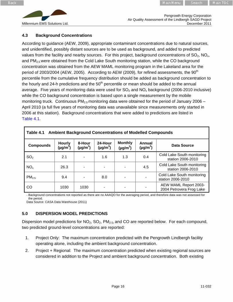
According to guidance (AEW, 2009), appropriate contaminant concentrations due to natural sources, and unidentified, possibly distant sources are to be used as background, and added to predicted values from the facility and nearby sources. For this project, background concentrations of SO2, NOx, and PM2.5 were obtained from the Cold Lake South monitoring station, while the CO background concentration was obtained from the AEW MAML monitoring program in the Lakeland area for the period of 2003/2004 (AEW, 2005). According to AEW (2009), for refined assessments, the 90th percentile from the cumulative frequency distribution should be added as background concentration to the hourly and 24-h predictions and the 50th percentile or mean should be added to the annual average. Five years of monitoring data were used for SO2 and NOx background (2006-2010 inclusive) while the CO background concentration is based upon a single measurement by the mobile monitoring truck. Continuous PM2.5 monitoring data were obtained for the period of January 2006 – April 2010 (a full five years of monitoring data was unavailable since measurements only started in 2006 at this station). Background concentrations that were added to predictions are listed in Table 4.1.
Table 4.1 Ambient Background Concentrations of Modelled Compounds
Compounds Hourly (µg/m3)
8-Hour (µg/m3)
24-Hour(µg/m3)
Monthly (µg/m3)
Annual (µg/m3)
Data Source
SO2 2.1 - 1.6 1.3 0.4 Cold Lake South monitoring
station 2006-2010
NOx 26.3 - - - 4.5 Cold Lake South monitoring
station 2006-2010
PM2.5 9.4 - 8.0 - - Cold Lake South monitoring station 2006-2010
CO 1030 1030 - - - AEW MAML Report 2003-2004 Petrovera Frog Lake
- Background concentrations not reported as there are no AAAQO for the averaging period, and therefore data was not assessed for the period.
Data Source: CASA Data Warehouse (2011)
5.0 DISPERSION MODEL PREDICTIONS
Dispersion model predictions for NO2, SO2, PM2.5, and CO are reported below. For each compound, two predicted ground-level concentrations are reported:
1. Project Only: The maximum concentration predicted with the Pengrowth Lindbergh facility operating alone, including the ambient background concentration.
2. Project + Regional: The maximum concentration predicted when existing regional sources are considered in addition to the Project and ambient background concentration. Both existing

Pengrowth Energy Corporation Air Quality Assessment of the Lindbergh SAGD Project Millennium EMS Solutions Ltd. December 2011
Page 17 11-032
and planned regional sources are included. The planned regional source is located at the edge of the project-inclusion area and is not a large source of emissions.
5.1 Sulphur Dioxide Model Predictions
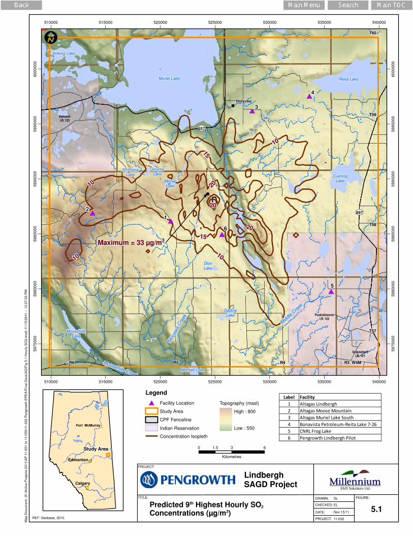
The CALPUFF modelling predictions for SO2 from the normal operation of the Project are listed in Table 5.1. The results show that all SO2 predictions at the Project property boundary line, as well as at the maximum points of impingement (MPOI), are below the AAAQO. All predictions presented in this section include background concentrations, as presented in Table 4.1.
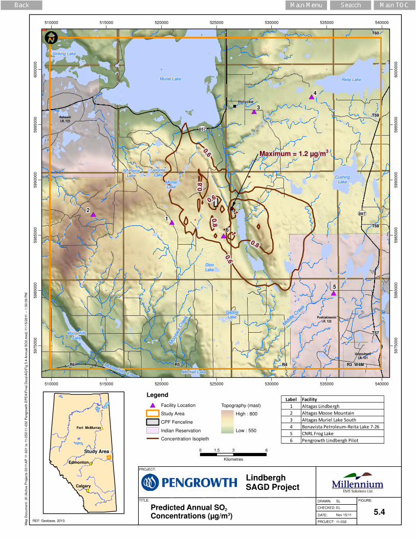
SO2 modelling results are also presented in the form of SO2 concentration contours (isopleths) in Figures 5.1 to 5.4, which show for the 9th highest hourly, 2nd highest daily, maximum monthly and annual predicted concentrations. The MPOI for the hourly, daily and monthly averaging periods is located northwest of the CPF. The annual MPOI occurs southeast of the CPF. As the steam boilers are the primary emitters of SO2 regionally, both scenarios yield the same results.
Table 5.1 Summary of Predicted SO2 Maximum Ground-Level Concentrations (g/m3)
Averaging Period
Scenario MPOI CPF
Boundary AAAQO (a)
99.9th Percentile 1-hour
Project Only 33 21 450
Project + Regional 33 21
2nd Highest 24-hour average
Project Only 15 7.0 125
Project + Regional 15 7.0
Maximum 30-day Average
Project Only 3.8 1.9 30
Project + Regional 3.8 1.9
Maximum Annual Average
Project Only 1.2 0.6 20
Project + Regional 1.2 0.7
(a) AEW 2011
#*
#*
#*
#*
#*
#*
KehewinI.R. 123
UnipouheosI.R. 121
Maximum = 33 µg/m3
PuskiakiweninI.R. 122
��657
��897
Holyoke
R5 R4R6
T59
T58
T57
R3 W4M
T60
Mid
dle
Cre
ek
Moosehills Creek
Moosw
a C
reek
St. PierreLake
JeromeLake
MichelLake
CushingLake
Sinking Lake
Reita LakeMuriel Lake
DionLake
GadoisLake
Mitchell Lake
MoosehillsLake
6
5
4
2
1
3
10
15
20
10
15
20
20
1010
510000
510000
515000
515000
520000
520000
525000
525000
530000
530000
535000
535000
540000
540000
59
75
00
0
59
75
00
0
59
80
00
0
59
80
00
0
59
85
00
0
59
85
00
0
59
90
00
0
59
90
00
0
59
95
00
0
59
95
00
0
60
00
00
0
60
00
00
0
5.1
SL
EL
Nov 15/11
11-032
LindberghSAGD Project
PROJECT:
DATE:
CHECKED:
DRAWN: FIGURE:
PROJECT:
TITLE:
I
REF: Geobase, 2010.
0 3 61.5
Kilometres
Legend
#* Facility Location
Study Area
CPF Fenceline
Indian Reservation
Concentration Isopleth
Study Area
Fort McMurray!(
Calgary
Edmonton
Topography (masl)
High : 800
Low : 550
Ma
p D
ocu
me
nt:
(K
:\A
ctive
Pro
jects
20
11
\AP
11
-00
1 t
o 1
1-0
50
\11
-03
2 P
en
gro
wth
EP
EA
\Fin
al D
ocs\A
Q\F
ig 5
.1 H
ou
rly S
O2
.mxd
) 11
/15
/20
11
--
12
:27
:53
PM
Predicted 9th Highest Hourly SO2
Concentrations (µg/m3)
Label Facility
1 Altagas Lindbergh
2 Altagas Moose Mountain
3 Altagas Muriel Lake South
4 Bonavista Petroleum-Reita Lake 7-26
5 CNRL Frog Lake
6 Pengrowth Lindbergh Pilot

#*
#*
#*
#*
#*
#*
KehewinI.R. 123
UnipouheosI.R. 121
Maximum = 15 µg/m3
PuskiakiweninI.R. 122
��657
��897
Holyoke
R5 R4R6
T59
T58
T57
R3 W4M
T60
Mid
dle
Cre
ek
Moosehills Creek
Moosw
a C
reek
St. PierreLake
JeromeLake
MichelLake
CushingLake
Sinking Lake
Reita LakeMuriel Lake
DionLake
GadoisLake
Mitchell Lake
MoosehillsLake
6
5
4
2
1
3
3.5 510
3.5
3.5
10
5
3.5
510000
510000
515000
515000
520000
520000
525000
525000
530000
530000
535000
535000
540000
540000
59
75
00
0
59
75
00
0
59
80
00
0
59
80
00
0
59
85
00
0
59
85
00
0
59
90
00
0
59
90
00
0
59
95
00
0
59
95
00
0
60
00
00
0
60
00
00
0
5.2
SL
EL
Nov 15/11
11-032
LindberghSAGD Project
PROJECT:
DATE:
CHECKED:
DRAWN: FIGURE:
PROJECT:
TITLE:
I
REF: Geobase, 2010.
0 3 61.5
Kilometres
Legend
#* Facility Location
Study Area
CPF Fenceline
Indian Reservation
Concentration Isopleth
Study Area
Fort McMurray!(
Calgary
Edmonton
Topography (masl)
High : 800
Low : 550
Ma
p D
ocu
me
nt:
(K
:\A
ctive
Pro
jects
20
11
\AP
11
-00
1 t
o 1
1-0
50
\11
-03
2 P
en
gro
wth
EP
EA
\Fin
al D
ocs\A
Q\F
ig 5
.2 D
aily
SO
2.m
xd
) 11
/15
/20
11
--
1:1
4:5
8 P
M
Predicted 2nd Highest Daily SO2
Concentrations (µg/m3)
Label Facility
1 Altagas Lindbergh
2 Altagas Moose Mountain
3 Altagas Muriel Lake South
4 Bonavista Petroleum-Reita Lake 7-26
5 CNRL Frog Lake
6 Pengrowth Lindbergh Pilot

#*
#*
#*
#*
#*
#*
KehewinI.R. 123
UnipouheosI.R. 121
Maximum = 3.8 µg/m3
PuskiakiweninI.R. 122
��657
��897
Holyoke
R5 R4R6
T59
T58
T57
R3 W4M
T60
Mid
dle
Cre
ek
Moosehills Creek
Moosw
a C
reek
St. PierreLake
JeromeLake
MichelLake
CushingLake
Sinking Lake
Reita LakeMuriel Lake
DionLake
GadoisLake
Mitchell Lake
MoosehillsLake
6
5
4
2
1
3
1.5
2
2.5
1.5
1.5
2
1.8
1.8
510000
510000
515000
515000
520000
520000
525000
525000
530000
530000
535000
535000
540000
540000
59
75
00
0
59
75
00
0
59
80
00
0
59
80
00
0
59
85
00
0
59
85
00
0
59
90
00
0
59
90
00
0
59
95
00
0
59
95
00
0
60
00
00
0
60
00
00
0
5.3
SL
EL
Nov 15/11
11-032
LindberghSAGD Project
PROJECT:
DATE:
CHECKED:
DRAWN: FIGURE:
PROJECT:
TITLE:
I
REF: Geobase, 2010.
0 3 61.5
Kilometres
Legend
#* Facility Location
Study Area
CPF Fenceline
Indian Reservation
Concentration Isopleth
Study Area
Fort McMurray!(
Calgary
Edmonton
Topography (masl)
High : 800
Low : 550
Ma
p D
ocu
me
nt:
(K
:\A
ctive
Pro
jects
20
11
\AP
11
-00
1 t
o 1
1-0
50
\11
-03
2 P
en
gro
wth
EP
EA
\Fin
al D
ocs\A
Q\F
ig 5
.3 M
on
thly
SO
2.m
xd
) 11
/15
/20
11
--
1:2
2:5
0 P
M
Predicted Maximum Monthly SO2
Concentrations (µg/m3)
Label Facility
1 Altagas Lindbergh
2 Altagas Moose Mountain
3 Altagas Muriel Lake South
4 Bonavista Petroleum-Reita Lake 7-26
5 CNRL Frog Lake
6 Pengrowth Lindbergh Pilot
#*
#*
#*
#*
#*
#*
KehewinI.R. 123
UnipouheosI.R. 121
Maximum = 1.2 µg/m3
PuskiakiweninI.R. 122
��657
��897
Holyoke
R5 R4R6
T59
T58
T57
R3 W4M
T60
Mid
dle
Cre
ek
Moosehills Creek
Moosw
a C
reek
St. PierreLake
JeromeLake
MichelLake
CushingLake
Sinking Lake
Reita LakeMuriel Lake
DionLake
GadoisLake
Mitchell Lake
MoosehillsLake
6
5
4
2
1
3
1
0.8
0.6
1
0.8
0.6
0.60.8
510000
510000
515000
515000
520000
520000
525000
525000
530000
530000
535000
535000
540000
540000
59
75
00
0
59
75
00
0
59
80
00
0
59
80
00
0
59
85
00
0
59
85
00
0
59
90
00
0
59
90
00
0
59
95
00
0
59
95
00
0
60
00
00
0
60
00
00
0
5.4
SL
EL
Nov 15/11
11-032
LindberghSAGD Project
PROJECT:
DATE:
CHECKED:
DRAWN: FIGURE:
PROJECT:
TITLE:
I
REF: Geobase, 2010.
0 3 61.5
Kilometres
Legend
#* Facility Location
Study Area
CPF Fenceline
Indian Reservation
Concentration Isopleth
Study Area
Fort McMurray!(
Calgary
Edmonton
Topography (masl)
High : 800
Low : 550
Ma
p D
ocu
me
nt:
(K
:\A
ctive
Pro
jects
20
11
\AP
11
-00
1 t
o 1
1-0
50
\11
-03
2 P
en
gro
wth
EP
EA
\Fin
al D
ocs\A
Q\F
ig 5
.4 A
nn
ua
l S
O2
.mxd
) 11
/15
/20
11
--
1:3
0:3
9 P
M
Predicted Annual SO2
Concentrations (µg/m3)
Label Facility
1 Altagas Lindbergh
2 Altagas Moose Mountain
3 Altagas Muriel Lake South
4 Bonavista Petroleum-Reita Lake 7-26
5 CNRL Frog Lake
6 Pengrowth Lindbergh Pilot

Pengrowth Energy Corporation Air Quality Assessment of the Lindbergh SAGD Project Millennium EMS Solutions Ltd. December 2011
Page 22 11-032
5.2 Nitrogen Dioxide Model Predictions
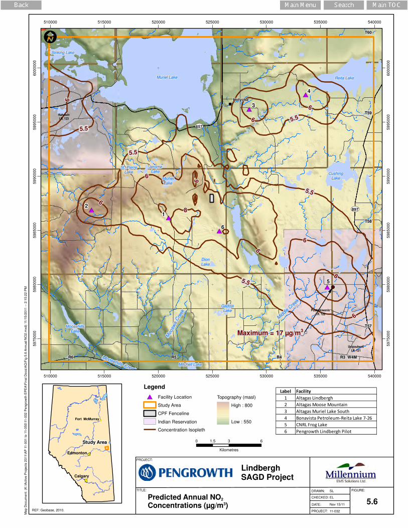
The CALPUFF modelling predictions for NO2 are listed in Table 5.2 and can also be seen in Figures 5.5 to 5.6, which show the contours of maximum NO2 concentration for the Project + Regional scenario for the hourly 99.9th percentile, 2nd highest 24-hour average, and maximum annual average concentrations, respectively. All predictions presented in this section include background concentrations, as presented in Table 4.1. NO2 concentration predictions using both the OLM and the Total Conversion Method are presented.
There are no exceedances of the AQ objectives for any averaging period when the OLM is used. The hourly MPOI occurs to the NE of the AltaGas Lindbergh facility. The annual maximum occurs near CNRL Frog Lake Facility.
Table 5.2 Summary of NO2 Maximum Predicted Ground-Level Concentrations (μg/m3)
Averaging Period Scenario MPOI CPF Boundary AAAQO
(a)
Total Conversion Method
99.9th Percentile
1-hour
Project Only 105 93 300
Project + Regional 623 139
Maximum Annual Average
Project Only 6.5 6.0 45
Project + Regional 17 7.1
Ozone Limiting Method
99.9th Percentile
1-hour
Project Only 105 93 300
Project + Regional 158 110
Maximum Annual Average
Project Only 6.5 6.0 45
Project + Regional 17 7.4
(a) AEW 2011

#*
#*
#*
#*
#*
#*
KehewinI.R. 123
UnipouheosI.R. 121
Maximum = 158 µg/m3
PuskiakiweninI.R. 122
��657
��897
Holyoke
R5 R4R6
T59
T58
T57
R3 W4M
T60
Mid
dle
Cre
ek
Moosehills Creek
Moosw
a C
reek
St. PierreLake
JeromeLake
MichelLake
CushingLake
Sinking Lake
Reita LakeMuriel Lake
DionLake
GadoisLake
Mitchell Lake
MoosehillsLake
6
5
4
2
1
3
8080
80
80
80
110
110
80
130 80
510000
510000
515000
515000
520000
520000
525000
525000
530000
530000
535000
535000
540000
540000
59
75
00
0
59
75
00
0
59
80
00
0
59
80
00
0
59
85
00
0
59
85
00
0
59
90
00
0
59
90
00
0
59
95
00
0
59
95
00
0
60
00
00
0
60
00
00
0
5.5
SL
EL
Nov 15/11
11-032
LindberghSAGD Project
PROJECT:
DATE:
CHECKED:
DRAWN: FIGURE:
PROJECT:
TITLE:
I
REF: Geobase, 2010.
0 3 61.5
Kilometres
Legend
#* Facility Location
Study Area
CPF Fenceline
Indian Reservation
Concentration Isopleth
Study Area
Fort McMurray!(
Calgary
Edmonton
Topography (masl)
High : 800
Low : 550
Ma
p D
ocu
me
nt:
(K
:\A
ctive
Pro
jects
20
11
\AP
11
-00
1 t
o 1
1-0
50
\11
-03
2 P
en
gro
wth
EP
EA
\Fin
al D
ocs\A
Q\F
ig 5
.5 H
ou
rly N
O2
.mxd
) 11
/15
/20
11
--
2:1
3:5
3 P
M
Predicted 9th Highest Hourly NO2
Concentrations (µg/m3)
Label Facility
1 Altagas Lindbergh
2 Altagas Moose Mountain
3 Altagas Muriel Lake South
4 Bonavista Petroleum-Reita Lake 7-26
5 CNRL Frog Lake
6 Pengrowth Lindbergh Pilot
#*
#*
#*
#*
#*
#*
KehewinI.R. 123
UnipouheosI.R. 121
Maximum = 17 µg/m3
PuskiakiweninI.R. 122
��657
��897
Holyoke
R5 R4R6
T59
T58
T57
R3 W4M
T60
Mid
dle
Cre
ek
Moosehills Creek
Moosw
a C
reek
St. PierreLake
JeromeLake
MichelLake
CushingLake
Sinking Lake
Reita LakeMuriel Lake
DionLake
GadoisLake
Mitchell Lake
MoosehillsLake
6
5
4
2
1
3
6
6
6
6
6
6
6
6
8
8
5.5
5.5
5.5
5.5
5.56
510000
510000
515000
515000
520000
520000
525000
525000
530000
530000
535000
535000
540000
540000
59
75
00
0
59
75
00
0
59
80
00
0
59
80
00
0
59
85
00
0
59
85
00
0
59
90
00
0
59
90
00
0
59
95
00
0
59
95
00
0
60
00
00
0
60
00
00
0
5.6
SL
EL
Nov 15/11
11-032
LindberghSAGD Project
PROJECT:
DATE:
CHECKED:
DRAWN: FIGURE:
PROJECT:
TITLE:
I
REF: Geobase, 2010.
0 3 61.5
Kilometres
Legend
#* Facility Location
Study Area
CPF Fenceline
Indian Reservation
Concentration Isopleth
Study Area
Fort McMurray!(
Calgary
Edmonton
Topography (masl)
High : 800
Low : 550
Ma
p D
ocu
me
nt:
(K
:\A
ctive
Pro
jects
20
11
\AP
11
-00
1 t
o 1
1-0
50
\11
-03
2 P
en
gro
wth
EP
EA
\Fin
al D
ocs\A
Q\F
ig 5
.6 A
nn
ua
l N
O2
.mxd
) 11
/15
/20
11
--
2:1
5:2
2 P
M
Predicted Annual NO2
Concentrations (µg/m3)
Label Facility
1 Altagas Lindbergh
2 Altagas Moose Mountain
3 Altagas Muriel Lake South
4 Bonavista Petroleum-Reita Lake 7-26
5 CNRL Frog Lake
6 Pengrowth Lindbergh Pilot

Pengrowth Energy Corporation Air Quality Assessment of the Lindbergh SAGD Project Millennium EMS Solutions Ltd. December 2011
Page 25 11-032
5.3 PM2.5 Model Predictions
The CALPUFF modelling predictions for PM2.5 are listed in Table 5.3, and the contours for the predicted 2nd highest daily concentrations are shown in Figure 5.7. The contours represent the Project + Regional scenario. All predictions presented in this section include background concentrations, as presented in Table 4.1. PM2.5 MPOIs are expected to occur of the west of the Lindbergh Pilot Facility.
Table 5.3 Summary of PM2.5 Maximum Ground-Level Concentrations (μg/m3)
Averaging Period Scenario MPOI CPF
Boundary AAAQO (a)
99.9th Percentile 1h Average
Project Only 13 13 80(b)
Project + Regional 55 26
2nd Highest 24-hour Average
Project Only 10 10 30
Project + Regional 23 12
(a) AEW 2011
(b) Guideline not an objective; not to be used to assess compliance.

#*
#*
#*
#*
#*
#*
KehewinI.R. 123
UnipouheosI.R. 121
Maximum = 23 µg/m3
PuskiakiweninI.R. 122
��657
��897
Holyoke
R5 R4R6
T59
T58
T57
R3 W4M
T60
Mid
dle
Cre
ek
Moosehills Creek
Moosw
a C
reek
St. PierreLake
JeromeLake
MichelLake
CushingLake
Sinking Lake
Reita LakeMuriel Lake
DionLake
GadoisLake
Mitchell Lake
MoosehillsLake
6
5
4
2
1
3
9
10
10
9
12
9
10
510000
510000
515000
515000
520000
520000
525000
525000
530000
530000
535000
535000
540000
540000
59
75
00
0
59
75
00
0
59
80
00
0
59
80
00
0
59
85
00
0
59
85
00
0
59
90
00
0
59
90
00
0
59
95
00
0
59
95
00
0
60
00
00
0
60
00
00
0
5.7
SL
EL
Nov 15/11
11-032
LindberghSAGD Project
PROJECT:
DATE:
CHECKED:
DRAWN: FIGURE:
PROJECT:
TITLE:
I
REF: Geobase, 2010.
0 3 61.5
Kilometres
Legend
#* Facility Location
Study Area
CPF Fenceline
Indian Reservation
Concentration Isopleth
Study Area
Fort McMurray!(
Calgary
Edmonton
Topography (masl)
High : 800
Low : 550
Ma
p D
ocu
me
nt:
(K
:\A
ctive
Pro
jects
20
11
\AP
11
-00
1 t
o 1
1-0
50
\11
-03
2 P
en
gro
wth
EP
EA
\Fin
al D
ocs\A
Q\F
ig 5
.7 D
aily
PM
25
.mxd
) 11
/15
/20
11
--
2:2
5:1
0 P
M
Predicted 2nd Highest Daily PM2.5
Concentrations (µg/m3)
Label Facility
1 Altagas Lindbergh
2 Altagas Moose Mountain
3 Altagas Muriel Lake South
4 Bonavista Petroleum-Reita Lake 7-26
5 CNRL Frog Lake
6 Pengrowth Lindbergh Pilot

Pengrowth Energy Corporation Air Quality Assessment of the Lindbergh SAGD Project Millennium EMS Solutions Ltd. December 2011
Page 27 11-032
5.4 CO Model Predictions
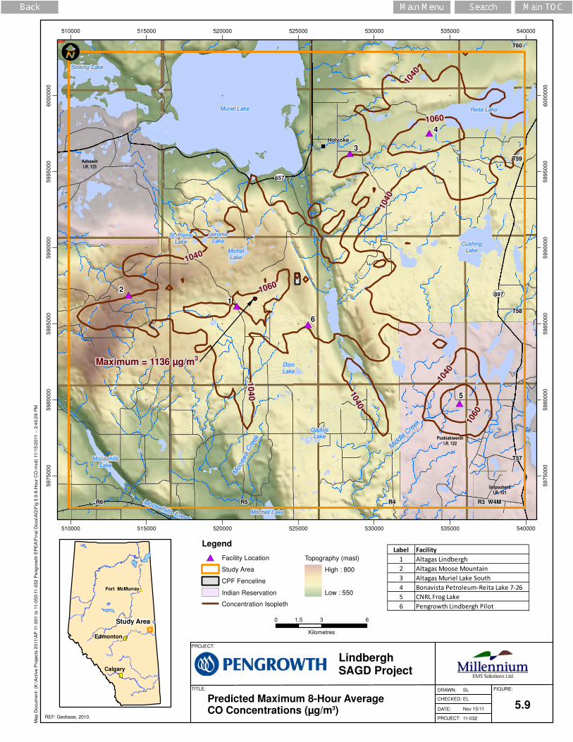
The CALPUFF modelling predictions for CO are listed in Table 5.4. All predictions presented in this section include background concentrations, as presented in Table 4.1. No exceedances of the AAAQO are predicted.
Figures 5.8 and 5.9 show the contours of predicted ground-level CO concentrations for hourly 99.9th percentile and maximum 8-hour averaging period, respectively. The MPOI occurs east of the Altagas Lindbergh facility, NW of the Pengrowth SAGD pilot and south of the Project, for both the 8-hour and hourly averaging periods.
Table 5.4 Summary of CO Maximum Ground-Level Concentrations (μg/m3)
Averaging Period Scenario MPOI CPF
Boundary AAAQO (a)
99.9th Percentile 1h-Average Project Only 1076 1076
15,000 Project + Regional 1187 1076
Maximum 8-hour Average Project Only 1078 1078
6,000 Project + Regional 1136 1078
(a) AEW 2011

#*
#*
#*
#*
#*
#*
KehewinI.R. 123
UnipouheosI.R. 121
Maximum = 1187 µg/m3
PuskiakiweninI.R. 122
��657
��897
Holyoke
R5 R4R6
T59
T58
T57
R3 W4M
T60
Mid
dle
Cre
ek
Moosehills Creek
Moosw
a C
reek
St. PierreLake
JeromeLake
MichelLake
CushingLake
Sinking Lake
Reita LakeMuriel Lake
DionLake
GadoisLake
Mitchell Lake
MoosehillsLake
6
5
4
2
1
3
1040
1040
1050
1050
1040
1050
1050
1040
1100
1040
1100
1040
510000
510000
515000
515000
520000
520000
525000
525000
530000
530000
535000
535000
540000
540000
59
75
00
0
59
75
00
0
59
80
00
0
59
80
00
0
59
85
00
0
59
85
00
0
59
90
00
0
59
90
00
0
59
95
00
0
59
95
00
0
60
00
00
0
60
00
00
0
5.8
SL
EL
Nov 15/11
11-032
LindberghSAGD Project
PROJECT:
DATE:
CHECKED:
DRAWN: FIGURE:
PROJECT:
TITLE:
I
REF: Geobase, 2010.
0 3 61.5
Kilometres
Legend
#* Facility Location
Study Area
CPF Fenceline
Indian Reservation
Concentration Isopleth
Study Area
Fort McMurray!(
Calgary
Edmonton
Topography (masl)
High : 800
Low : 550
Ma
p D
ocu
me
nt:
(K
:\A
ctive
Pro
jects
20
11
\AP
11
-00
1 t
o 1
1-0
50
\11
-03
2 P
en
gro
wth
EP
EA
\Fin
al D
ocs\A
Q\F
ig 5
.8 H
ou
rly C
O.m
xd
) 11
/15
/20
11
--
2:3
0:5
8 P
M
Predicted 9th Highest Hourly COConcentrations (µg/m3)
Label Facility
1 Altagas Lindbergh
2 Altagas Moose Mountain
3 Altagas Muriel Lake South
4 Bonavista Petroleum-Reita Lake 7-26
5 CNRL Frog Lake
6 Pengrowth Lindbergh Pilot
#*
#*
#*
#*
#*
#*
KehewinI.R. 123
UnipouheosI.R. 121
Maximum = 1136 µg/m3
PuskiakiweninI.R. 122
��657
��897
Holyoke
R5 R4R6
T59
T58
T57
R3 W4M
T60
Mid
dle
Cre
ek
Moosehills Creek
Moosw
a C
reek
St. PierreLake
JeromeLake
MichelLake
CushingLake
Sinking Lake
Reita LakeMuriel Lake
DionLake
GadoisLake
Mitchell Lake
MoosehillsLake
6
5
4
2
1
3
1060
1040
1040
10
40
1040
1060
1040
1060
1040
510000
510000
515000
515000
520000
520000
525000
525000
530000
530000
535000
535000
540000
540000
59
75
00
0
59
75
00
0
59
80
00
0
59
80
00
0
59
85
00
0
59
85
00
0
59
90
00
0
59
90
00
0
59
95
00
0
59
95
00
0
60
00
00
0
60
00
00
0
5.9
SL
EL
Nov 15/11
11-032
LindberghSAGD Project
PROJECT:
DATE:
CHECKED:
DRAWN: FIGURE:
PROJECT:
TITLE:
I
REF: Geobase, 2010.
0 3 61.5
Kilometres
Legend
#* Facility Location
Study Area
CPF Fenceline
Indian Reservation
Concentration Isopleth
Study Area
Fort McMurray!(
Calgary
Edmonton
Topography (masl)
High : 800
Low : 550
Ma
p D
ocu
me
nt:
(K
:\A
ctive
Pro
jects
20
11
\AP
11
-00
1 t
o 1
1-0
50
\11
-03
2 P
en
gro
wth
EP
EA
\Fin
al D
ocs\A
Q\F
ig 5
.9 8
-Ho
ur
CO
.mxd
) 11
/15
/20
11
--
2:4
0:2
9 P
M
Predicted Maximum 8-Hour AverageCO Concentrations (µg/m3)
Label Facility
1 Altagas Lindbergh
2 Altagas Moose Mountain
3 Altagas Muriel Lake South
4 Bonavista Petroleum-Reita Lake 7-26
5 CNRL Frog Lake
6 Pengrowth Lindbergh Pilot

Pengrowth Energy Corporation Air Quality Assessment of the Lindbergh SAGD Project Millennium EMS Solutions Ltd. December 2011
Page 30 11-032
6.0 UPSET MODELLING
According to AEW (2009), the impact due to emergency and upset conditions must be considered in environmental assessments for air quality.
Three upset scenarios were considered:
1. Loss of power requiring the use of an emergency generator. The estimated run time for the emergency generator is 4 outages per year, for 3 hours in duration, plus a monthly test of approximately 5 hours duration. Emission parameters are listed in Table 6.1.
2. Loss of boilers of boilers and all produced gas going to flare. This event is estimated to occur 8 times per year, with a maximum duration of 4 hours each.
3. Regulator failure on let-down station for pipeline fuel gas to boilers. This is estimated to occur once per year, with an anticipated duration of 15 minutes.
The emission details and modelling parameters for the two flaring upsets (Upset Case # 2 and Upset Case # 3) are presented in Table 6.2. The flare stack and emission parameters are derived from engineering estimates with pseudo stack parameters calculated using the ERCB Flare Spreadsheet (ERCB, 2010).
Table 6.1 Emergency Generator Parameters and Emissions
Parameter Upset Case 1
UTM Coordinates – Easting (m) 524840
UTM Coordinates –Northing (m) 5987928
Elevation (m ASL) 698
Stack Height (m) 4.0
Stack Diameter (m) 0.203
Exit Velocity (m/s) 63.1
Exit Temperature (K) 779
SO2 Emission Rate (g/s) 0.19
NOx Emission Rate (g/s) 2.9
CO Emission Rate (g/s) 0.61
PM2.5 Emission Rate (g/s) 0.20

Pengrowth Energy Corporation Air Quality Assessment of the Lindbergh SAGD Project Millennium EMS Solutions Ltd. December 2011
Page 31 11-032
Table 6.2 Flare Stack and Emission Parameters
Parameter Upset Case 2 Upset Case 3
UTM Coordinates – Easting (m) 525037 525037
UTM Coordinates –Northing (m) 5988177 5988177
Elevation (m ASL)
Flare Height (m) 40.0 40.0
Exit Diameter (m) 0.356 0.356
Pseudo Release Height (m) 41.7 51.5
Pseudo Exit Velocity (m/s) 0.325 1.8
Pseudo Diameter (m) 13.4 20.8
Exit Temperature (K) 1267 1282
SO2 Emission Rate (g/s) 11.3 0.04
NOx Emission Rate (g/s) 0.47 0.655
Max. Flaring Duration (min) 240 15
Lower Heating Value (MJ/m3) 256 33.56
Flow Rate (103m3/d @ 15oC and 101.325 kPa)
50.8 518.9
Mole Fraction:
H2O 3.38E-02 8.40E-05
H2 0.0 0.0
He 0.0 0.0
N2 3.83E-04 7.00E-03
CO2 2.26E-01 3.60E-03
H2S 7.11E-03 0.00E+00
CH4 7.28E-01 9.89E-01
C2H6 2.20E-05 4.00E-04
C3H8 3.30E-05 1.00E-04
i-C4H10 5.30E-05 1.00E-04
n-C4H10 3.39E-04 1.00E-04
i-C5H12 9.62E-04 0.0
n-C5H12 1.04E-03 0.0
n-C6H14 7.84E-04 0.0
C7+ 1.24E-03 0.0
CO 0.0 0.0
NH3 0.0 0.0
Total 1.0 1.0
The results of Upset Case #1 are presented in Table 6.3 and indicate that no exceedances of SO2, NO2, CO or PM2.5 are introduced by the operation of the emergency generator. The presented

Pengrowth Energy Corporation Air Quality Assessment of the Lindbergh SAGD Project Millennium EMS Solutions Ltd. December 2011
Page 32 11-032
predictions include all Project sources, regional sources and background concentrations, as well upset emissions.
Results from upset flaring scenarios are presented in Table 6.4. The predicted SO2 hourly
concentration for Upset Case #2 is 29 g/m3. This value is lower than the predicted concentration for normal operations, as presented in Section 5.1. The Project steam boilers are the primary source of SO2 emissions in the region. This flaring scenario occurs when there is a loss of the boilers, and the gas is diverted to the flare. The higher combustion temperature results in a more complete destruction of the H2S and the higher stack provides better dispersion.
The predicted hourly NO2 concentration for Upset Case #3 is 158 g/m3, which is below the AAAQO
of 300 g/m3.
Table 6.3 Predicted 9th Highest Hourly Concentration from Emergency Generator Operation –
Upset Case #1 (including Project and Regional Sources) (g/m3)
Species Predicted Concentration AAAQO(a)
SO2 47 450
NO2 170 300
CO 1187 15,000
PM2.5 57 80(b) (a) AEW 2011 (b) Guideline, not objective.
Table 6.4 Predicted Hourly Concentration from Upset Flaring (including Project and Regional
Sources) (g/m3)
Species Case #2 – Boiler Loss Case #3 – Regulator
Let-Down AAAQO(a)
SO2 29 - (b) 450
NO2 - (b) 158 300 (a) AEW 2011 (b) Emission rate low (see Table 6.3) so modelling results are not presented. Flaring contribution to regional predictions not-detectable.

Pengrowth Energy Corporation Air Quality Assessment of the Lindbergh SAGD Project Millennium EMS Solutions Ltd. December 2011
Page 33 11-032
7.0 SUMMARY AND CONCLUSIONS
The CALMET meteorological model and the CALPUFF dispersion models were used to assess the dispersion of SO2, NOx, PM2.5, and CO emissions associated with the expected operation of the Lindbergh SAGD facility using maximum emission rates. Sources of these emissions from all industrial facilities within a 40 x 40 km area centered on the Lindbergh site were included in the modelling.
The facility has a total of six stacks with continuous emissions. The results of dispersion modelling showed there were no predicted exceedances for SO2, NO2, PM2.5 or CO for any averaging period. The use of an emergency upset generator is not expected to introduce any exceedances of hourly AAAQOs for (SO2, NO2, CO or PM2.5). Upset flaring will not introduce any exceedances of hourly SO2 or NO2 AAAQOs. Thus, the air quality during operation of the Lindbergh SAGD facility in normal and upset conditions is expected to be acceptable.
8.0 CLOSURE
This report has been prepared for the exclusive use of Pengrowth Energy Corporation, its affiliates and authorized users for specific application to this Project. The environmental investigation was conducted in accordance with the proposed work scope prepared for this site, and generally accepted assessment practices. No other warranty, expressed or implied, is made.
Respectfully submitted,
Millennium EMS Solutions Ltd. Prepared by: Reviewed by:
Elizabeth Logan, M.A.Sc., E.I.T. Randy Rudolph, M.Sc. Air Quality Engineer Principal

Pengrowth Energy Corporation Air Quality Assessment of the Lindbergh SAGD Project Millennium EMS Solutions Ltd. December 2011
Page 34 11-032
9.0 REFERENCES
AEW (Alberta Environment and Water). 2005. Air Quality Monitoring – The Lakeland Area. Spring and Fall of 2003 and 2004 - Final Report. April 27, 2005.
AEW, 2009. Air Quality Model Guideline. http://environment.gov.ab.ca/info/library/8151.pdf
AEW, 2011. Alberta Ambient Air Quality Objectives and Guidelines. Issued in June, 15 2011.
CASA, 2010. Clean Air Strategic Alliance. Data Warehouse [Online] Accessed November 2010. Available at the website: http://www.casadata.org/reports/
CASA, 2011. Clean Air Strategic Alliance. Data Warehouse [Online] Accessed October 2011. Available at the website: http://www.casadata.org/reports/
CCME. 1998. National Emission Guideline for Commercial/Industrial Boilers and Heaters. CCME NOX/VOC Management Plan, N306 Multistakeholders Working Group and Steering Committee Canadian Environmental Quality Guidelines. Winnipeg, MB: CCME.
CCME. 2000. Canada-Wide Standards for Particulate Matter (PM) and Ozone. Endorsed June 5-6, 2000. Quebec, PQ.
ERCB (Energy Resources Conservation Board). 2010. ERCBflare Ver 1.05, March 5, 2010. Flaring Dispersion Modelling Spreadsheet for ERCB Directive 60 – Upstream Petroleum Industry Flaring, Incinerating, and Venting.
Osum Oil Sands Corp., 2009. Application for Approval of the Taiga Project. Prepared by Matrix Solutions Inc. Calgary, AB.
Pengrowth Corporation (2010). Lindbergh SAGD Pilot Project: Project Update and Supplemental Information Responses. Submitted to Alberta Environment. Prepared by Millennium EMS Solutions Ltd. Edmonton, AB.
Stantec, 2010. Stantec. Air Quality Update Report Associated with the Pengrowth Corporation Lindbergh Facility. June 25, 2009.
U.S. EPA. 1998. United States Environmental Protection Agency. AP-42 Emission Factors. Fifth Edition. http://www.epa.gov/ttn/chief/ap42/
U.S. EPA. 2011. Compilation of Air Pollutant Emission Factors AP-42, 5th Edition (on-line version, including all updates. Research Triangle Park, NC. http://www.epa.gov/ttn/chief/ap42/
Waukesha, 2008. Dresser Waukesha. Data Sheet for F18GL. Turbocharged and Intercooled, Lean Combustion, Six Cylinder, 4-Cycle Gas Fuelled Engine.

Pengrowth Energy Corporation Appendix A: Air Quality Modelling Settings Millennium EMS Solutions Ltd. December 2011
11-032
APPENDIX A: AIR QUALITY MODELLING SETTINGS
Pengrowth Energy Corporation Appendix A: Air Quality Modelling Settings Millennium EMS Solutions Ltd. December 2011
Page A-i 11-032
Table of Contents Page Table of Contents .................................................................................................................................... i List of Tables .......................................................................................................................................... ii
1.0 INTRODUCTION ........................................................................................................................ 1
2.0 CALMET MODEL OPTIONS ...................................................................................................... 1
2.1 Wind Field Options (Input Group 5) ........................................................................................ 1
2.2 Meteorological Data Options (Input Group 4 and 6) ............................................................... 1
2.3 Surface Meteorology ............................................................................................................... 6
2.4 Fifth Generation NCAR/Penn State Mesoscale Model (MM5) ................................................ 6
2.5 Geophysical Parameters ......................................................................................................... 6
2.5.1 Land Use ......................................................................................................................... 6
2.5.2 Terrain ............................................................................................................................. 8
2.5.3 Anthropogenic Heat Flux Parameter ............................................................................... 8
3.0 CALPUFF MODEL OPTIONS .................................................................................................... 9
4.0 REFERENCES ......................................................................................................................... 22

Pengrowth Energy Corporation Appendix A: Air Quality Modelling Settings Millennium EMS Solutions Ltd. December 2011
Page A-ii 11-032
List of Tables Page
Table A2-1 Wind Field Options and Parameters (Input Group 5) ...................................................... 2
Table A2-2 Wind Field Options and Parameters (Input Group 4) ...................................................... 3
Table A2-3 Mixing Height Parameters (Input Group 6) ..................................................................... 4
Table A2-4 Temperature Parameters ................................................................................................ 5
Table A2-5 Surface Variables Associated with Land Use Characteristics ......................................... 7
Table A3-1 Assumed Gas Properties ................................................................................................ 9
Table A3-2 Assumed Particulate Matter Properties ........................................................................... 9
Table A3-3 Assumed Wet Deposition Parameters ............................................................................ 9
Table A3-4 Input Groups in the CALPUFF Control File ................................................................... 10
Table A3-5 General Run Control Parameters (Input Group 1) ........................................................ 11
Table A3-6 Technical Options (Input Group 2) ................................................................................ 12
Table A3-7 Species List-Chemistry Options (Subgroup 3a) ............................................................ 14
Table A3-8 Map Projection Grid Control Parameters (Input Group 4) ............................................. 14
Table A3-9 Sub-Grid Scale Complex Terrain Inputs (Input Group 6a) ............................................ 15
Table A3-10 Dry Deposition Parameters for Gases (Input Group 7) ................................................. 16
Table A3-11 Size Parameters for Dry Deposition of Particles (Input Group 8) .................................. 17
Table A3-12 Miscellaneous Dry Deposition Parameters (Input Group 9) .......................................... 17
Table A3-13 Wet Deposition Parameters .......................................................................................... 17
Table A3-14 Chemistry Parameters (Input Group 11) ....................................................................... 18
Table A3-15 Miscellaneous Dispersion and Computational Parameters (Input Group 12) ............... 19

Pengrowth Energy Corporation Appendix A: Air Quality Modelling Settings Millennium EMS Solutions Ltd. December 2011
Page A-1 11-032
1.0 INTRODUCTION
CALMET and CALPUFF models were used for the air quality assessment. Both of the models are described in detail by Scire et al (2000) and Scire and Escoffier-Czaja (2004), and are recommended by Alberta Environment and Water (AEW) for regulatory air quality assessments (AEW, 2009).
This appendix summarizes the CALMET and CALPUFF settings and compares to the default parameter settings. Where a discrepancy between set value and default occurs, justification is given.
2.0 CALMET MODEL OPTIONS
2.1 Wind Field Options (Input Group 5)
Within the CALMET model, there are a number of options for calculating the modelling domain wind field. Similarity theory is used to extrapolate surface winds to upper layers.
The maximum overland radius of influence for the surface layer is 5 km. The radius is 15 km at upper levels. Additionally, the minimum radius of influence for the wind field interpolation is 0.1 km, and radius of influence is set to 15 km for terrain features. The wind field options for the dispersion meteorological component of the model are described in Table A2-1.
2.2 Meteorological Data Options (Input Group 4 and 6)
Hourly surface heat fluxes, as well as the observed morning and afternoon temperature soundings, were used to calculate mixing heights. The minimum and maximum mixing heights allowed were 50 m and 3,000 m, respectively.
The inverse distance-squared method, which was recommended by Dean and Snyder (1977) and Wei and McGuinness (1976), was used to interpolate air temperature, with a radius of influence of 500 km. A larger radius produces a more realistic temperature field, particularly at the surface.
The meteorological data options, mixing height, precipitation, and temperature parameters that were used in the Project assessment are outlined in Table A2-2, Table A2-3, and Table A2-4, respectively.
The following provides rationale for the use of non-default model parameters:
IEXTRP: MM5 meteorology was used as the only source of meteorological data and for that reason there is no extrapolation for surface wind observations.
IPROG: MM5 data were used.
FEXTR2: there is no extrapolation – this option is used only when IEXTRP = 3 or -3, whereas IEXTRP = 1 was used in the project.
ISURFT: this option is used only when ITPROG=2 (no surface and upper air observations – use MM5 for surface and upper air data).

Pengrowth Energy Corporation Appendix A: Air Quality Modelling Settings Millennium EMS Solutions Ltd. December 2011
Page A-2 11-032
NOOBS: no upper air stations used.
IRHPROG: used as NOOBS = 2.
ICLOUD: Cloud data calculated from MM5 data gives more realistic gridded cloud cover.
FCORIO: reflects northern latitude around the project.
ITPROG: use MM5 data.
Table A2-1 Wind Field Options and Parameters (Input Group 5)
Parameter Default Current Description
Wind Field Model Options
IWFCOD 1 1 Model selection variable – Diagnostic wind module
IFRADJ 1 1 Compute Froude number adjustment (Yes = 1)
IKINE 0 0 Compute kinematic effects (No = 0)
IOBR 0 0 Use O’Brien procedure for adjustment of the vertical velocity (No)
ISLOPE 1 1 Compute slope flow effects (Yes)
IEXTRP -4 -1 Extrapolate surface wind observations to upper layers (similarity theory used with layer 1 data at upper air stations ignored)
ICALM 0 0 Extrapolate surface winds even if calm (No)
BIAS NZ*0 0,0,0,0,0,0,0,
0 Layer-dependent biases modifying the weights of surface and upper air stations
RMIN2 4.0 4.0 Minimum distance (km) from nearest upper air station to surface station for which extrapolation of surface winds at surface station will be allowed
IPROG 0 14 Use gridded prognostic wind field model output fields as input to the diagnostic wind field model (14=use winds from MM5.DAT file as initial guess field)
ISTEPPGS 3600 3600 Time-step (seconds) of the prognostic model input data
IGFMET 0 0 Use coarse CALMET fields as initial guess fields (overwrites IGF based on prognostic wind fields if any)
Radius of Influence Parameters LVARY F F Use varying radius of influence (F - False)
RMAX1 - 50 Maximum radius of influence over land in the surface layer (km)
RMAX2 - 150 Maximum radius of influence over land aloft (km)
RMAX3 - 300 Maximum radius of influence over water (km)
Other Wind Field Input Parameters RMIN 0.1 0.1 Minimum radius of influence used in the wind field interpolation (km)
TERRAD - 15.0 Radius of influence of terrain features (km)
R1 - 25 Relative weighting of the first guess field and observations in the surface layer (km)
R2 - 75 Relative weighting of the first guess field and observations in the layers aloft (km)
RPROG - 54.0 Relative weighting parameter of the prognostic wind field data (km)
DIVLIM 5.0E-6 5.0E-6 Maximum acceptable divergence in the divergence minimization procedure

Pengrowth Energy Corporation Appendix A: Air Quality Modelling Settings Millennium EMS Solutions Ltd. December 2011
Page A-3 11-032
Table A2-1 Wind Field Options and Parameters (Input Group 5)
Parameter Default Current Description
NITER 50 50 Maximum number of iterations in the divergence minimization procedure
NSMTH (NZ) 2,(mxnz-
1)*4
2, 28, 28, 28, 28, 28, 28,
28 Number of passes in the smoothing procedure
NINTR2 99 99, 99, 99, 99, 99, 99,
99, 99
Maximum number of stations used in each layer for the interpolation of data to a grid point(number 12 is bigger than number of stations, then all stations are used)
CRITFN 1.0 1.0 Critical Froude number
ALPHA 0.1 0.1 Empirical factor controlling the influence of kinematic effects
FEXTR2(NZ) nz*0.0 1, 1.7, 2.2, 3, 3.9, 5.1, 6.3,
7.2
Multiplicative scaling factor for extrapolation of surface observations to upper layers
NBAR 0 0 Number of barriers to interpolation of the wind fields
KBAR NZ 8 Level (1 to NZ) up to which barriers apply
Diagnostic Module Data Input Options
IDIOPTI 0 0 Surface temperature (0 = compute internally from hourly surface observation)
ISURFT -1 -1 Surface meteorological station to use for the surface temperature (parameter ISURFT= -1 is for 2-D spatially varying surface temperatures)
IDIOPT2 0 0 Domain-averaged temperature lapse (0 = compute internally from hourly surface observation)
IUPT -1 -1 Upper air station to use for the domain-scale lapse rate (-1 to use 2-D spatially varying lapse rate)
ZUPT 200 200 Depth through which the domain-scale lapse rate is computed (m)
IDIOPT3 0 0 Domain-averaged wind components
IUPWND -1 -1 Upper air station to use for the domain-scale winds
ZUPWND 1.0, 1000 1.0, 1000 Bottom and top of layer through which domain-scale winds are computed (m)
IDIOPT4 0 0 Observed surface wind components for wind field module
IDIOPT5 0 0 Observed upper air wind components for wind field module
Table A2-2 Wind Field Options and Parameters (Input Group 4)
Parameter Default Current Description
NOOBS 0 2 Use surface and overwater stations (no upper air observations) Use MM4/MM5/M3D for upper air data
Number of Surface & Precipitation Meteorological Stations
NSSTA - 0 Number of surface stations
NPSTA - -1 use of MM5/M3D precipitation data
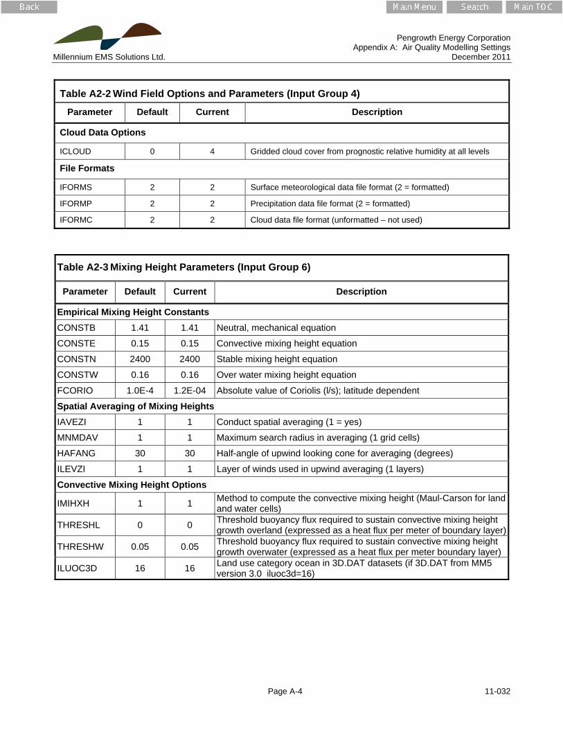
Pengrowth Energy Corporation Appendix A: Air Quality Modelling Settings Millennium EMS Solutions Ltd. December 2011
Page A-4 11-032
Table A2-2 Wind Field Options and Parameters (Input Group 4)
Parameter Default Current Description
Cloud Data Options
ICLOUD 0 4 Gridded cloud cover from prognostic relative humidity at all levels
File Formats
IFORMS 2 2 Surface meteorological data file format (2 = formatted)
IFORMP 2 2 Precipitation data file format (2 = formatted)
IFORMC 2 2 Cloud data file format (unformatted – not used)
Table A2-3 Mixing Height Parameters (Input Group 6)
Parameter Default Current Description
Empirical Mixing Height Constants
CONSTB 1.41 1.41 Neutral, mechanical equation
CONSTE 0.15 0.15 Convective mixing height equation
CONSTN 2400 2400 Stable mixing height equation
CONSTW 0.16 0.16 Over water mixing height equation
FCORIO 1.0E-4 1.2E-04 Absolute value of Coriolis (l/s); latitude dependent
Spatial Averaging of Mixing Heights
IAVEZI 1 1 Conduct spatial averaging (1 = yes)
MNMDAV 1 1 Maximum search radius in averaging (1 grid cells)
HAFANG 30 30 Half-angle of upwind looking cone for averaging (degrees)
ILEVZI 1 1 Layer of winds used in upwind averaging (1 layers)
Convective Mixing Height Options
IMIHXH 1 1 Method to compute the convective mixing height (Maul-Carson for land and water cells)
THRESHL 0 0 Threshold buoyancy flux required to sustain convective mixing height growth overland (expressed as a heat flux per meter of boundary layer)
THRESHW 0.05 0.05 Threshold buoyancy flux required to sustain convective mixing height growth overwater (expressed as a heat flux per meter boundary layer)
ILUOC3D 16 16 Land use category ocean in 3D.DAT datasets (if 3D.DAT from MM5 version 3.0 iluoc3d=16)

Pengrowth Energy Corporation Appendix A: Air Quality Modelling Settings Millennium EMS Solutions Ltd. December 2011
Page A-5 11-032
Table A2-3 Mixing Height Parameters (Input Group 6)
Parameter Default Current Description
Other Mixing Heights Variables
DPTMIN 0.001 0.001 Minimum potential temperature lapse rate in the stable layer above the current convective missing height (oK/m)
DZZI 200 200 Depth of layer above current convective mixing height through which lapse rate is computed (m)
ZIMIN 50 50 Minimum overland mixing height (m)
ZIMAX 3000 3000 Maximum overland mixing height (m)
ZIMINW 50 50 Minimum over-water mixing height (m)
ZIMAXW 3000 3000 Maximum over-water mixing height (m)
Overwater Surface Fluxes Method and Parameters
ICOARE 10 10 COARE with no wave parameterization
DSHELF 0 0 Coastal/Shallow water length scale
IWARM 0 0 COARE warm layer computation (0=off)
ICOOL 0 0 COARE cool skin layer computation (0=off)
Relative Humidity Parameters
IRHPROG 0 1 3D relative humidity from observations or from prognostic data (0= use RH NOOBS = 0,1)
Table A2-4 Temperature Parameters
Parameter Default Current Description
Temperature Parameters
ITPROG 0 2 Use Surface stations (no upper air observations), Use MM5/M3D for upper air data (only if NOOBS = 0,1)
IRAD 1 1 Interpolation type (1 = 1/R)
TRADKM 500 500 Radius of influence for temperature interpolation (km)
NUMTS 5 5 Maximum number of stations to include in temperature interpolation
IAVET 1 1 Conduct spatial averaging of temperatures (1 = yes)
TGDEFB -0.0098 -0.0098 Default temperature gradient below the mixing height over water (oK/m)
TGDEFA -0.0045 -0.0045 Default temperature gradient above the mixing height over water (oK/m)
JWAT1 - 99 Beginning land use categories for temperature interpolation over water (disabled)
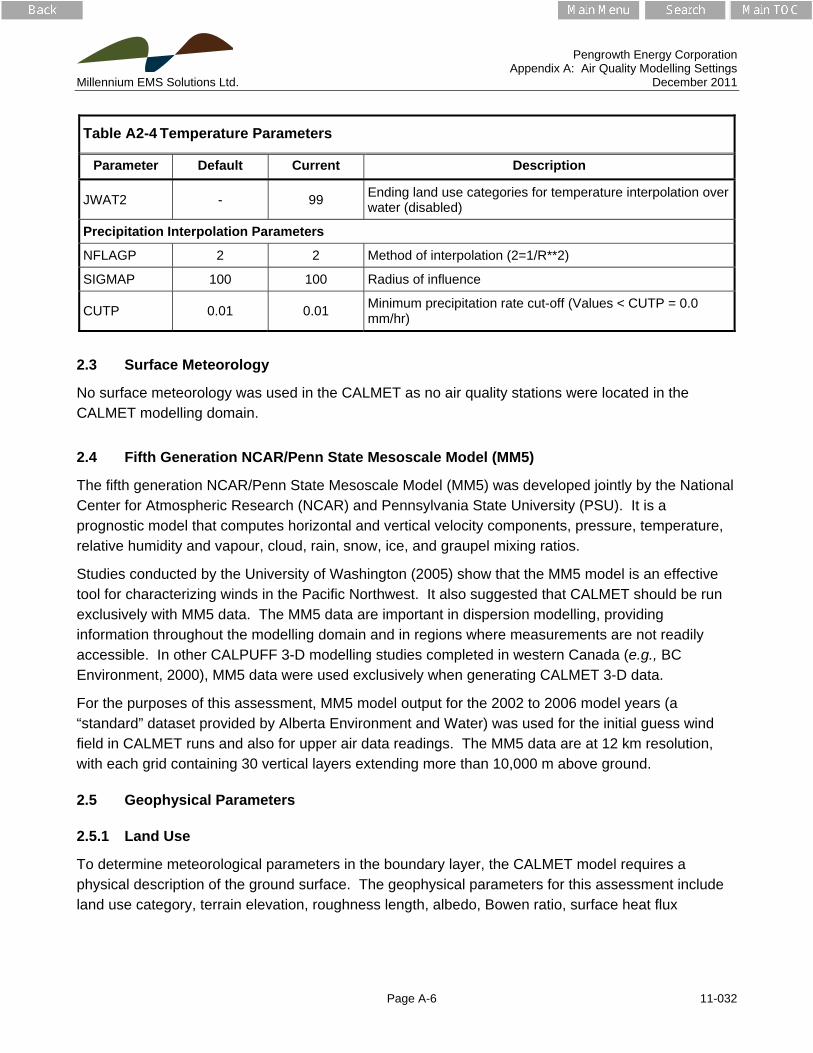
Pengrowth Energy Corporation Appendix A: Air Quality Modelling Settings Millennium EMS Solutions Ltd. December 2011
Page A-6 11-032
Table A2-4 Temperature Parameters
Parameter Default Current Description
JWAT2 - 99 Ending land use categories for temperature interpolation over water (disabled)
Precipitation Interpolation Parameters
NFLAGP 2 2 Method of interpolation (2=1/R**2)
SIGMAP 100 100 Radius of influence
CUTP 0.01 0.01 Minimum precipitation rate cut-off (Values < CUTP = 0.0 mm/hr)
2.3 Surface Meteorology
No surface meteorology was used in the CALMET as no air quality stations were located in the CALMET modelling domain.
2.4 Fifth Generation NCAR/Penn State Mesoscale Model (MM5)
The fifth generation NCAR/Penn State Mesoscale Model (MM5) was developed jointly by the National Center for Atmospheric Research (NCAR) and Pennsylvania State University (PSU). It is a prognostic model that computes horizontal and vertical velocity components, pressure, temperature, relative humidity and vapour, cloud, rain, snow, ice, and graupel mixing ratios.
Studies conducted by the University of Washington (2005) show that the MM5 model is an effective tool for characterizing winds in the Pacific Northwest. It also suggested that CALMET should be run exclusively with MM5 data. The MM5 data are important in dispersion modelling, providing information throughout the modelling domain and in regions where measurements are not readily accessible. In other CALPUFF 3-D modelling studies completed in western Canada (e.g., BC Environment, 2000), MM5 data were used exclusively when generating CALMET 3-D data.
For the purposes of this assessment, MM5 model output for the 2002 to 2006 model years (a “standard” dataset provided by Alberta Environment and Water) was used for the initial guess wind field in CALMET runs and also for upper air data readings. The MM5 data are at 12 km resolution, with each grid containing 30 vertical layers extending more than 10,000 m above ground.
2.5 Geophysical Parameters
2.5.1 Land Use
To determine meteorological parameters in the boundary layer, the CALMET model requires a physical description of the ground surface. The geophysical parameters for this assessment include land use category, terrain elevation, roughness length, albedo, Bowen ratio, surface heat flux

Pengrowth Energy Corporation Appendix A: Air Quality Modelling Settings Millennium EMS Solutions Ltd. December 2011
Page A-7 11-032
parameter, anthropogenic heat flux and leaf area index (LAI). Values for all land use parameters except land use category and elevation were determined for the following periods:
Winter – January 1 to March 31 and November 15 to December 31;
Spring – April 1 to June 14;
Summer – June 15 to August 31; and
Fall – September 1 to November 14.
The geophysical parameters for all periods are summarized in Table A2-5 below.
Table A2-5 Surface Variables Associated with Land Use Characteristics
LUC Description Roughness
Length Zo (m)Albedo
Bowen Ratio
Heat FluxAnthropogenic
Heat Flux Leaf Area
Index (LAI)
Winter
42 Evergreen Forest
(Coniferous) 0.90 0.35 1.50 0.15* 0 4.00
52 Lakes 0.05* 0.70* 0.50* 1.00 0 0
61 Forested Wetland 0.70 0.43 1.50 0.15* 0 1.0
62 Nonforested Wetland 0.70 0.43 1.50 0.15* 0 1.0
Spring
42 Evergreen Forest
(Coniferous) 0.90 0.25 0.70 0.15 0 4.00
52 Lakes 0.01 0.20 0.10 1.00 0 0
61 Forested Wetland 0.80 0.15 0.50 0.15 0 1.2
62 Nonforested Wetland 0.80 0.15 0.50 0.15 0 1.2
Summer
42 Evergreen Forest
(Coniferous) 1.00 0.12 1.20 0.15 0 4.00
52 Lakes 0.0001 0.10 0.05 1.00 0 0
61 Forested Wetland 1.0 0.12 0.40 0.25 0 2.0
62 Nonforested Wetland 1.0 0.12 0.40 0.25 0 2.0
Fall
42 Evergreen Forest
(Coniferous) 1.00 0.12 1.00 0.15 0 4.00
52 Lakes 0.0001 0.14 0.05 1.00 0 0
61 Forested Wetland 0.90 0.12 0.40 0.25 0 1.5
62 Nonforested Wetland 0.90 0.12 0.40 0.25 0 1.5
* Value recommended by TRC for perennial snow. Also the default value for cropland and pasture, rangeland, forest, and barren land.

Pengrowth Energy Corporation Appendix A: Air Quality Modelling Settings Millennium EMS Solutions Ltd. December 2011
Page A-8 11-032
The CALMET modelling domain was described using four land use categories. A category was assigned to each 0.5 km x 0.5 km grid cell based on the most prevalent land use type according to those described by Cihlar and Beaubien (1998). These descriptive categories were then grouped into broader classifications, which were provided by CALMET. The Land Use Categories were defined by referencing topographic 1:50,000 maps of the area.
Each land use category was assigned summer, fall, winter, and spring values of roughness length, albedo, Bowen Ratio, anthropogenic and soil flux parameters, and leaf area index.
The geotechnical parameters were largely the default values (recommended by PCRAMMET; US EPA 1995a).
2.5.2 Terrain
Topographic elevations for the terrain were obtained from the Shuttle Radar Topography Mission (SRTM – 3 Arc Second – 90 m), which is a joint project between the National Geo-spatial-Intelligence Agency (NGA) and the National Aeronautics and Space Administration (NASA) (SRTM, 2005). The CALMET pre-processor program, TERREL, was used to extract and format terrain data.
2.5.3 Anthropogenic Heat Flux Parameter
The urban heat island effect is a result of the interaction of several factors, including the absorption of heat during the day by surfaces such as asphalt roads, concrete pavements, and roofs, which is then radiated out into the atmosphere at night, and the release of heat from the tailpipes of vehicles and ventilation stacks from buildings. The latter source of heat is especially significant in winter months. The study of the anthropogenic heat flux in Nagoya, Japan revealed an additional anthropogenic heat flux from the city centre of about 50 W/m2 during the winter months (Yamaguchi et al, 2004). The anthropogenic heat flux in Tokyo exceeded 400 W/m2 in summer during the daytime, and the maximum value occurred in winter (1,590 W/m2). In the suburbs of Tokyo, the heat flux from houses reached about 30 W/m2 (CGER, 1997).
For modelling purposes, the anthropogenic heat flux is usually considered to be zero due to lack of measurements in a given area. However, PCRAMMET (US EPA, 1995a) recognizes that in areas with high population densities or energy use, such as an industrial facility, anthropogenic flux may not always be negligible. An anthropogenic heat flux of about 10 W/m2 in summer, 15 W/m2 in spring and fall, and 30 W/m2 in winter was assumed for urban areas. It was also assumed that the anthropogenic heat flux from open mine surfaces was 5 W/m2 during the whole year. The anthropogenic heat flux elsewhere was assumed to be zero.

Pengrowth Energy Corporation Appendix A: Air Quality Modelling Settings Millennium EMS Solutions Ltd. December 2011
Page A-9 11-032
3.0 CALPUFF MODEL OPTIONS
Assumed gas and particulate matter properties are listed in Tables A3-1 to A3-3. The CALPUFF dispersion model is a tool that uses a range of user specified options. The CALPUFF control file defines 17 input groups as identified in Table A3-4.
Table A3-1 Assumed Gas Properties
SO2 NO NO2 HNO3
Diffusivity (cm2/s) 0.115 0.186 0.141 0.108
Alpha Star (a*) 1000 1.0 1.0 1.0
Reactivity 8 2 8 18
Mesophyll Resistance (s/cm) 0 94 5 0
Henry's Law Coefficient 0.0332 21.5 4.09 10x10-8
Table A3-2 Assumed Particulate Matter Properties
SO4 NO3 PM2.5
Geometric mass mean diameter ((µm) 0.48 0.48 0.98
Geometric standard deviation (µm) 2.0 2.0 1.8
Table A3-3 Assumed Wet Deposition Parameters
Scavenging Coefficient
(s-1)
SO2 SO4 NO NO2 HNO3 NO3 PM2.5
Liquid 3.2 x 10⁻⁵ 1 x 10⁻⁴ 2.9 x 10⁻⁵ 5.1 x 10⁻⁵ 6 x 10⁻⁵ 1 x 10⁻⁴ 1 x 10⁻⁴
Frozen 0 3 x 10⁻⁵ 0 0 0 3 x 10⁻⁵ 3 x 10⁻⁵

Pengrowth Energy Corporation Appendix A: Air Quality Modelling Settings Millennium EMS Solutions Ltd. December 2011
Page A-10 11-032
Table A3-4 Input Groups in the CALPUFF Control File
Input Group
Description Applicable to the Project
0 Input and output file names Yes
1 General run control parameters Yes
2 Technical options Yes
3 Species list Yes
4 Grid control parameters Yes
5 Output options Yes
6 Sub grid scale complex terrain inputs No
7 Dry deposition parameters for gases Yes
8 Dry deposition parameters for particles Yes
9 Miscellaneous dry deposition for parameters Yes
10 Wet deposition parameters Yes
11 Chemistry parameters Yes
12 Diffusion and computational parameters Yes
13 Point source parameters Yes
14 Area source parameters Yes
15 Line source parameters No
16 Volume source parameters Yes
17 Discrete receptor information Yes
The chemistry option was invoked in CALPUFF since SO2 and NOx sources are involved in this assessment. This option was switched on when dealing with the following eight species: SO2, SO4, NO, NO2, HNO3, NO3, CO, and primary PM2.5, but was switched off for the modelling runs that assessed ambient VOC concentrations.
The CALPUFF input parameters were selected according to the default values, with some exceptions. For the simulation of building downwash, the PRIME method was used for buildings within Project fence lines; building downwash was not considered for non-Project facilities.
Tables A3-5 to A3-15 identify the input parameters, default options, and values used for the current project. Non-default parameters were used as follows:
MBDW: PRIME method used for plume downwash – PRIME method is considered more advanced and it is recommended by modelling guidelines AEW(2009a)

Pengrowth Energy Corporation Appendix A: Air Quality Modelling Settings Millennium EMS Solutions Ltd. December 2011
Page A-11 11-032
MCHEM: RIVAD/ARM3 chemistry used for chemical transformations. In several tests conducted to date, the results have shown no significant differences between the modelling results obtained with MESOPUFF II and RIVAD/ARM3 chemistry (http://www.src.com/calpuff/FAQ-answers.htm#3.3.6).
MREG: unnecessary as this is not a U.S. application
Diffusivity: based on current literature (Seinfeld and Pandis, 2006)
PPC values were based on values in the ADEPT2 model developed for dispersion modelling in Alberta.
Table A3-5 General Run Control Parameters (Input Group 1)
Parameter Default Current Description
METRUN 0 0 All model periods in met file(s) will be run
IBYR - 2002 Starting year
IBMO - 1 Starting month
IBDY - 1 Starting day
IBHR - 0 Starting hour
IBMIN - 0 Starting minute
IBSEC - 0 Starting second
IEYR - 2007 Ending year
IEMO - 1 Ending month
IEDY - 1 Ending day
IEMIN - 0 Ending minute
IESEC - 0 Ending second
XBTZ - 7.0 Base time zone (MST = 7.0)
NSECDT - 3600 Length of run (seconds)
NSPEC 5 8 Number of chemical species
NSE 3 5 Number of chemical species to be emitted
ITEST 2 2 Program is executed after SETUP phase
MRESTART 0 0 Does not read or write a restart file
NRESPD 0 0 Restart file written only at last period
METFM 1 1 Meteorological data format 1= CALMET binary file (CALMET.MET)

Pengrowth Energy Corporation Appendix A: Air Quality Modelling Settings Millennium EMS Solutions Ltd. December 2011
Page A-12 11-032
Table A3-5 General Run Control Parameters (Input Group 1)
Parameter Default Current Description
MPRFFM 1 1 Meteorological profile data format
AVET 60 60 Averaging time (minutes)
PGTIME 60 60 PG Averaging time (minutes)
Table A3-6 Technical Options (Input Group 2)
Parameter Default Current Description
MGAUSS 1 1 Gaussian distribution used in near field
MCTADJ 3 3 Terrain adjustment method (3 = Partial plume path adjustment)
MCTSG 0 0 Subgrid-scale complex terrain (0 = not modelled)
MSLUG 0 0 Near-field puffs not modelled as elongated
MTRANS 1 1 Transitional plume rise modelled
MTIP 1 1 Stack tip downwash used (MTIP=0 for upset flaring)
MRISE 1 1 Briggs plume rise for point sources not subjected to building downwash
MBDW 1 2 Method used to simulate building downwash (2 = PRIME method)
MSHEAR 0 0 Vertical wind shear not modelled
MSPLIT 0 0 Puff splitting is not allowed
MCHEM 1 3 Transformation rates computed internally using RIVID/ARM3 scheme
MAQCHEM 0 0 Aqueous phase transformation not modelled
MWET 1 1 Wet removal modelled
MDRY 1 1 Dry deposition modelled
MTILT 0 0 Gravitational settling (plume tilt) not modelled
MDISP 3 3 Method used to compute dispersion coefficients - PG dispersion coefficients for RURAL areas (computed using the ISCST multi-segment approximation) and MP coefficients in urban areas
MTURBVW 3 3 Use both v and w from PROFILE.DAT to compute y and z (n/a)

Pengrowth Energy Corporation Appendix A: Air Quality Modelling Settings Millennium EMS Solutions Ltd. December 2011
Page A-13 11-032
Table A3-6 Technical Options (Input Group 2)
Parameter Default Current Description
MDISP2 3 3
Back-up method used to compute dispersion when measured turbulence data are missing (used only if MDISP = 1 or 5) This parameter is not used because MDISP = 3 for Connacher Great Divide.
MTAULY 0 0 Draxler default 617.284 (s) used for Lagrangian timescale for Sigma-y (used only if MDISP=1,2 or MDISP2=1,2)
MTAUADV 0 0 Method used for Advective-Decay timescale for Turbulence (used only if MDISP=2 or MDISP2=2)
MCTURB 1 1 Standard CALPUFF subroutines used to compute turbulence sigma-v & sigma-w using micrometeorological variables(Used only if MDISP = 2 or MDISP2 = 2)
MROUGH 0 0 PG y and z not adjusted for roughness
MPARTL 1 1 partial plume penetration of elevated inversion
MPARTLBA 1 1 partial plume penetration of elevated inversion (buoyant area sources)
MTINV 0 0 Strength of temperature inversion computed from default gradients
MPDF 0 0 PDF not used for dispersion under convective conditions
MSGTIBL 0 0 Sub-grid TIBL module not used for shore line
MBCON 0 0 Boundary conditions (concentration) not modelled
MSOURCE 0 0 No Individual source contributions saved
MFOG 0 0 Do not configure for FOG model output
MREG 1 0 Do not test options specified to see if they conform to regulatory values

Pengrowth Energy Corporation Appendix A: Air Quality Modelling Settings Millennium EMS Solutions Ltd. December 2011
Page A-14 11-032
Table A3-7 Species List-Chemistry Options (Subgroup 3a)
CSPEC Modelled
(0=no, 1=yes)
Emitted
(0=no, 1=yes)
Dry deposition (0=none,
1=computed gas,
2=computed particle, 3=user-specified)
Output group Number
SO2 1 1 1 0
SO4-2 1 0 2 0
NO 1 1 1 0
NO2 1 1 1 0
HNO3 1 0 1 0
NO3- 1 0 2 0
PM2.5 1 1 2 0
CO 1 1 0 0
Table A3-8 Map Projection Grid Control Parameters (Input Group 4)
Parameter Default Current Description
PMAP UTM UTM Map projection: Universal Transverse Mercator
IUTMZN - 12 UTM Zone (1 to 60)
UTMHEM N N Northern hemisphere UTM projection
DATUM WGS-84 NAR-B NIMA Datum Region - Canada
NX - 90 Number of X grid cells in meteorological grid
NY 90 Number of Y grid cells in meteorological grid
NZ - 8 Number of vertical layers in meteorological grid
DGRIDKM - 0.5 Grid spacing (km)
ZFACE - 0,20,40,80,
160,320,600,1400,3000
Cell face heights in meteorological grid (m)
XORIGKM - 505.7 Reference X coordinate for SW corner of grid cell (1,1) of meteorological grid (km)
YORIGKM - 5965.0 Reference Y coordinate for SW corner of grid cell (1,1) of meteorological grid (km)

Pengrowth Energy Corporation Appendix A: Air Quality Modelling Settings Millennium EMS Solutions Ltd. December 2011
Page A-15 11-032
Table A3-8 Map Projection Grid Control Parameters (Input Group 4)
Parameter Default Current Description
IBCOMP - 1 X index of lower left corner of the computational grid
JBCOMP - 1 Y index of lower left corner of the computational grid
IECOMP - 40 X index upper right corner of the computational grid
JECOMP - 40 Y index upper right corner of the computational grid
LSAMP T F Sampling grid is not used
IBSAMP - 1 X index of lower left corner of the sampling grid
JBSAMP - 1 Y index of lower left corner of the sampling grid
IESAMP - 40 X index of upper right corner of the sampling grid
JESAMP - 40 Y index of upper right corner of the sampling grid
MESHDN 1 1 Nesting factor of the sampling grid
Table A3-9 Sub-Grid Scale Complex Terrain Inputs (Input Group 6a)
Parameter Default Current Description
NHILL 0 0 Number of terrain features
NCTREC 0 0 Number of special complex terrain receptors
MHILL - 0 Input terrain and receptor data for CTSG hills input in CTDM format
XHILL2M 1 1 Conversion factor for changing horizontal dimensions to metres
ZHILL2M 1 1 Conversion factor for changing vertical dimensions to metres
XCTDMKM - 0 X origin of CTDM system relative to CALPUFF coordinate system (km)
YCTDMKM - 0 Y origin of CTDM system relative to CALPUFF coordinate system (km)

Pengrowth Energy Corporation Appendix A: Air Quality Modelling Settings Millennium EMS Solutions Ltd. December 2011
Page A-16 11-032
Table A3-10 Dry Deposition Parameters for Gases (Input Group 7)
Species Default Current Description
SO2
0.1509 0.115 Diffusivity (cm2/s) (Seinfeld and Pandis, 2006; US Forest Services)
1000.0 1000. Alpha star
8.0 8.0 Reactivity
0.0 0.0 Mesophyll resistance (s/cm)
0.4 0.0332 Henry’s Law coefficient
NO
- 0.186 Diffusivity (cm2/s) (Seinfeld and Pandis, 2006; US Forest Services)
- 1.0 Alpha star
- 2. Reactivity
- 94. Mesophyll resistance (s/cm)
- 21.5 Henry’s Law coefficient
NO2
0.1656 0.141 Diffusivity (cm2/s) (Seinfeld and Pandis, 2006; US Forest Services)
1.0 1.0 Alpha star
8.0 8. Reactivity
5.0 5. Mesophyll resistance (s/cm)
3.5 4.09 Henry’s Law coefficient
HNO3
0.1628 0.108 Diffusivity (cm2/s) (Seinfeld and Pandis, 2006; US Forest Services)
1.0 1.0 Alpha star
18.0 18. Reactivity
0.0 0. Mesophyll resistance (s/cm)
0.00000008 0.0000001 Henry’s Law coefficient
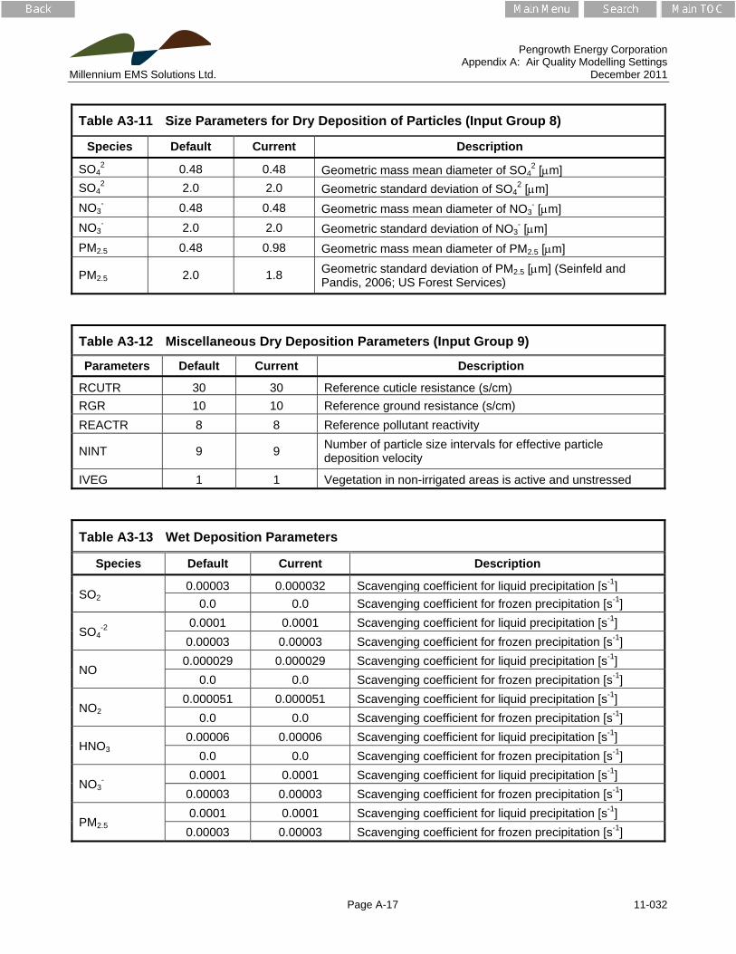
Pengrowth Energy Corporation Appendix A: Air Quality Modelling Settings Millennium EMS Solutions Ltd. December 2011
Page A-17 11-032
Table A3-11 Size Parameters for Dry Deposition of Particles (Input Group 8)
Species Default Current Description
SO42 0.48 0.48 Geometric mass mean diameter of SO4
2 [m]
SO42 2.0 2.0 Geometric standard deviation of SO4
2 [m]
NO3- 0.48 0.48 Geometric mass mean diameter of NO3
- [m]
NO3- 2.0 2.0 Geometric standard deviation of NO3
- [m]
PM2.5 0.48 0.98 Geometric mass mean diameter of PM2.5 [m]
PM2.5 2.0 1.8 Geometric standard deviation of PM2.5 [m] (Seinfeld and Pandis, 2006; US Forest Services)
Table A3-12 Miscellaneous Dry Deposition Parameters (Input Group 9)
Parameters Default Current Description
RCUTR 30 30 Reference cuticle resistance (s/cm)
RGR 10 10 Reference ground resistance (s/cm)
REACTR 8 8 Reference pollutant reactivity
NINT 9 9 Number of particle size intervals for effective particle deposition velocity
IVEG 1 1 Vegetation in non-irrigated areas is active and unstressed
Table A3-13 Wet Deposition Parameters
Species Default Current Description
SO2 0.00003 0.000032 Scavenging coefficient for liquid precipitation [s-1]
0.0 0.0 Scavenging coefficient for frozen precipitation [s-1]
SO4-2
0.0001 0.0001 Scavenging coefficient for liquid precipitation [s-1]
0.00003 0.00003 Scavenging coefficient for frozen precipitation [s-1]
NO 0.000029 0.000029 Scavenging coefficient for liquid precipitation [s-1]
0.0 0.0 Scavenging coefficient for frozen precipitation [s-1]
NO2
0.000051 0.000051 Scavenging coefficient for liquid precipitation [s-1]
0.0 0.0 Scavenging coefficient for frozen precipitation [s-1]
HNO3 0.00006 0.00006 Scavenging coefficient for liquid precipitation [s-1]
0.0 0.0 Scavenging coefficient for frozen precipitation [s-1]
NO3-
0.0001 0.0001 Scavenging coefficient for liquid precipitation [s-1]
0.00003 0.00003 Scavenging coefficient for frozen precipitation [s-1]
PM2.5 0.0001 0.0001 Scavenging coefficient for liquid precipitation [s-1]
0.00003 0.00003 Scavenging coefficient for frozen precipitation [s-1]

Pengrowth Energy Corporation Appendix A: Air Quality Modelling Settings Millennium EMS Solutions Ltd. December 2011
Page A-18 11-032
Table A3-14 Chemistry Parameters (Input Group 11)
Parameters Default Current Description
MOZ 1 1 Monthly background ozone value
BCKO3 12*80 32.03; 32.62; 35.75; 39.72; 36.39; 31.45; 24.56; 20.58; 19.97; 23.57; 28.08; 26.51
Background monthly ozone concentration (ppb)
BCKNH3 12*10 12*0.22 Background ammonia concentration (ppb)
RNITE1 0.2 0.2 Nighttime NO2 loss rate in percent/hour
RNITE2 2 2 Nighttime NOX loss rate in percent/hour
RNITE3 2 2 Nighttime HNO3 loss rate in percent/hour
MH202 1 1 Background H2O2 concentrations
BCKH202 12*1 12*1 Background monthly H2O2 concentrations (Aqueous phase transformations not modelled)
BCKPMF - -
Fine particulate concentration for Secondary Organic Aerosol Option (used only if MCHEM=4 in Connacher Great Divide MCHEM =3)
OFRAC - - Organic fraction of fine particulate for SOA Option (used only if MCHEM=4)
VCNX - - VOC/NOx ratio for SOA Option (used only if MCHEM=4)

Pengrowth Energy Corporation Appendix A: Air Quality Modelling Settings Millennium EMS Solutions Ltd. December 2011
Page A-19 11-032
Table A3-15 Miscellaneous Dispersion and Computational Parameters (Input Group 12)
Parameters Default Current Description
SYDEP 550 550 Horizontal size of a puff in metres beyond which the time dependant dispersion equation of Heffter is used
MHFTSZ 0 0 Do not use Heffter formulas for sigma z
JSUP 5 5 Stability class used to determine dispersion rates for puffs above boundary layer
CONK1 0.01 0.01 Vertical dispersion constant for stable conditions
CONK2 0.1 0.1 Vertical dispersion constant for neutral/stable conditions
TBD 0.5 0.5 Use ISC transition point for determining the transition point between the Schulman-Scire to Huber-Snyder Building Downwash scheme
IURB1 10 10 Lower range of land use categories for which urban dispersion is assumed
IURB2 19 19 Upper range of land use categories for which urban dispersion is assumed
ILANDUIN 20 20 Land use category for modelling domain
ZOIN 0.25 0.25 Roughness length in metres for modelling domain
XLAIIN 3.0 3.0 Leaf area index for modelling domain
ELEVIN 0.0 334 Elevation above sea level
XLATIN -999 57.0 North latitude of station in degrees
XLONIN -999 111.0 South latitude of station in degrees
ANEMHT 10 10 Anemometer height in metres
ISIGMAV 1 1 Sigma-v is read for lateral turbulence data
IMIXCTDM 0 0 Predicted mixing heights are used
XMXLEN 1 1 Maximum length of emitted slug in meteorological grid units
XSAMLEN 1 1 Maximum travel distance of slug or puff in meteorological grid units during one sampling unit
MXNEW 99 99 Maximum number of puffs or slugs released from one source during one time step
MXSAM 99 99 Maximum number of sampling steps during one time step for a puff or slug
NCOUNT 2 2 Number of iterations used when computing the transport wind for a sampling step that includes transitional plume rise

Pengrowth Energy Corporation Appendix A: Air Quality Modelling Settings Millennium EMS Solutions Ltd. December 2011
Page A-20 11-032
Table A3-15 Miscellaneous Dispersion and Computational Parameters (Input Group 12)
Parameters Default Current Description
SYMIN 1 1 Minimum sigma y in metres for a new puff or slug
SZMIN 1 1 Minimum sigma z in metres for a new puff or slug
CDIV 0.0, 0.0 0.0, 0.0 Divergence criteria for dw/dz in met cells
NLUTIBL 4 4 Search radius for nearest land and water cells
WSCALM 0.5 0.5 Minimum wind speed allowed for non-calm conditions (m/s)
XMAXZI 3000 3000 Maximum mixing height in metres
XMINZI 50 50 Minimum mixing height in metres
WSCAT
1.54 1.54 wind speed category 1 [m/s]
3.09 3.09 wind speed category 2 [m/s]
5.14 5.14 wind speed category 3 [m/s]
8.23 8.23 wind speed category 4 [m/s]
10.80 10.80 wind speed category 5 [m/s]
PTG0 0.020 0.020 potential temperature gradient for E stability [K/m]
0.035 0.035 potential temperature gradient for F stability [K/m]
SL2PF 10 10 Slug-to-puff transition criterion factor equal to sigma y/length of slug
NSPLIT 3 3 Number of puffs that result every time a puff is split
IRESPLIT Hour 17=1 Hour 17=1 Time(s) of day when split puffs are eligible to be split once again
ZISPLIT 100 100 Minimum allowable last hour’s mixing height for puff splitting
ROLDMAX 0.25 0.25 Maximum allowable ratio of last hour’s mixing height and maximum mixing height experienced by the puff for puff splitting
NSPLITH 5 5 Number of puff that result every time a puff is split (nsplith = 5 means that 1 puff splits into 5)
SYSPLITH 1 1 Minimum sigma-y of puff before it may be horizontally split
SHSPLITH 2 2 Minimum puff elongation rate due to wind shear before it may be horizontally split
CNSPLITH 1.0E-7 1.0E-7 Minimum concentration of each species in puff before it may be horizontally split

Pengrowth Energy Corporation Appendix A: Air Quality Modelling Settings Millennium EMS Solutions Ltd. December 2011
Page A-21 11-032
Table A3-15 Miscellaneous Dispersion and Computational Parameters (Input Group 12)
Parameters Default Current Description
EPSSLUG 1.00E-04 1.00E-04 Fractional convergence criterion for numerical SLUG sampling iteration
EPSAREA 1.00E-06 1.00E-06 Fractional convergence criterion for numerical AREA sampling iteration
DRISE 1.0 1.0 Trajectory step length for numerical rise
HTMINBC 500 500 Minimum height (m) to which BC puffs are mixed as they are emitted at the release point if greater than this minimum
RSAMPBC 10 10 Search radius (km) about a receptor for sampling nearest BC puff
MDEPBC 1 1 Near-surface depletion adjustment to concentration profile used when sampling BC puffs - Adjust concentration for depletion
Stability Class
Parameter
SVMIN SWMIN
Minimum turbulence (v) (m/s) Minimum turbulence (w) (m/s)
Land Water Land Water
A 0.50 0.37 0.20 0.20
B 0.50 0.37 0.12 0.12
C 0.50 0.37 0.08 0.08
D 0.50 0.37 0.06 0.06
E 0.50 0.37 0.03 0.03
F 0.50 0.37 0.016 0.016
Stability Class
Parameter
PLX0 PPC
Wind speed profile exponent Plume path coefficient
A 0.21 0.8
B 0.21 0.7
C 0.23 0.6
D 0.40 0.5
E 0.62 0.4
F 0.50 0.35

Pengrowth Energy Corporation Appendix A: Air Quality Modelling Settings Millennium EMS Solutions Ltd. December 2011
Page A-22 11-032
4.0 REFERENCES
AEW (Alberta Environment and Water). 2009. Air Quality Model Guideline. Prepared by A. Idriss and F. Spurrell, Climate Change, Air and Land Policy Branch. http://environment.gov.ab.ca/info/library/8151.pdf. 44 pp.
BOVAR Environmental (1996a). Meteorology Observations in the Athabasca Oil Sands Region. Report. No. 3 prepared for Suncor Inc., Oil Sands Group, and Syncrude Canada Ltd.
BOVAR Environmental (1996b). Ambient Air Quality Predictions in the Athabasca Oil Sands Region. Report. No. 4 prepared for Suncor Inc., Oil Sands Group, and Syncrude Canada Ltd.
British Columbia Ministry of Environment, Lands and Parks (BC Environment). 2000. Submission by BC Environment to Washington State Energy Facility Site Evaluation Council Regarding the Proposed Sumas Energy Project. Victoria, BC.
CEMA (Cumulative Environmental Management Association). 2005. NOx Dispersion and Chemistry Assumptions in the CALPUFF Model. Prepared by RWDI Air Inc.
Cihlar, J. and J. Beaubien. 1998. Land Cover of Canada, Version 1.1. Special Publication, NBIOME Project. Produced by the Canadian Center for Remote Sensing, Canadian Forest Service, Natural Resources Canada. Available on CD from the Canadian Centre for Remote Sensing. Ottawa, ON.
CGER (Center for Global Environmental Research).1997, Distribution of Urban Anthropogenic Heat In Tokyo Based on Very Precise Digital Land Use Data. CGER-D019(CD)-’97. Tsukuba JAPAN.
Dean, J.D. and W.M. Snyder. 1977. Temporally and Areally Distributed Rainfall. Journal of Irrigation and Drainage Division 103:221-229.
Holtslag, A.A.M. and A.P. van Ulden. 1983. A Simple Scheme for Daytime Estimates of Surface Fluxes from Routine Weather Data. Journal of Climate and Applied Meteorology 22: 517-529.
Scire, J. and C. Escoffier-Czaja. 2004. CALPUFF Training Course, Canadian Prairie and Northern Section of the Air and Waste Management Association. Calgary, AB
Scire, J.S., D.G. Strimaitis and R.J. Yamartino. 2000. A User’s Guide for the CALPUFF Model (Version 5.0). Earth Technologies Inc. Concord, MA.
Seinfeld J.H. and Pandis S.N. (2006) Atmospheric Chemistry and Physics – From Air Pollution to Climate Change; Second Edition –John Wiley & Sons Inc.

Pengrowth Energy Corporation Appendix A: Air Quality Modelling Settings Millennium EMS Solutions Ltd. December 2011
Page A-23 11-032
Shuttle Radar Technology Mission (SRTM). 2005. “Finished”. Pre-defined areas of 3 arc second (90 meter) SRTM "Finished" data in SRTM format, on DVD; covers the globe between 60° N and 56° S latitude. The SRTM Format is created from the SRTM DTED® Level 1 "Finished" product supplied by National Geospace-Intelligence Agency. Available at: http://edc.usgs.gov/products/elevation/srtmbil.html.
TRC (TRC solutions).2010. http://www.src.com/calpuff/FAQ-questions.htm. Accessed April 2010.
United States Environmental Protection Agency (US EPA). 1995a. PCRAMMET User’s Guide. US EPA, Office of Air Quality Planning and Standards. Research Triangle Park, NC.
United States Environmental Protection Agency (US EPA). 1995b. User’s Guide for the Industrial Source Complex (ISC3) Dispersion Models, Volume II – Description of Model Algorithms. Office of Air Quality Planning and Standards. Research Triangle Park, NC.
University of Washington. 2005. Pacific Northwest MM5 Verification Statistics. Available at: (http://www.atmos.washington.edu/mm5rt/verify.html).
US Forest Service. 2011. http://www.fs.fed.us/rm/landscapes/Solutions/Mole.shtml Date: Accessed April 2011.
Wei, T.C. and J.L. McGuinness. 1976. Reciprocal Distance Squared Method, A Computer Technique for Estimated Areal Precipitation. ARS NC-8. US Department of Agriculture. Washington, DC.
Yamaguchi, Y., S. Kato and K. Okamato. 2004. Surface Heat Flux Analysis in Urban Areas Using ATER and MODIS Data. GIS-IDEAS Hanoi, 2004 Symposium by Japan-Vietnam Geoinformatics Consortium. Available at: http://gisws.media.osaka-cu.ac.jp/gisideas04

Pengrowth Energy Corporation Air Quality Appendix B - Lindbergh SAGD Project Millennium EMS Solutions Ltd. December 2011
11-032
APPENDIX B: CCME EMISSION RATE SAMPLE CALCULATION
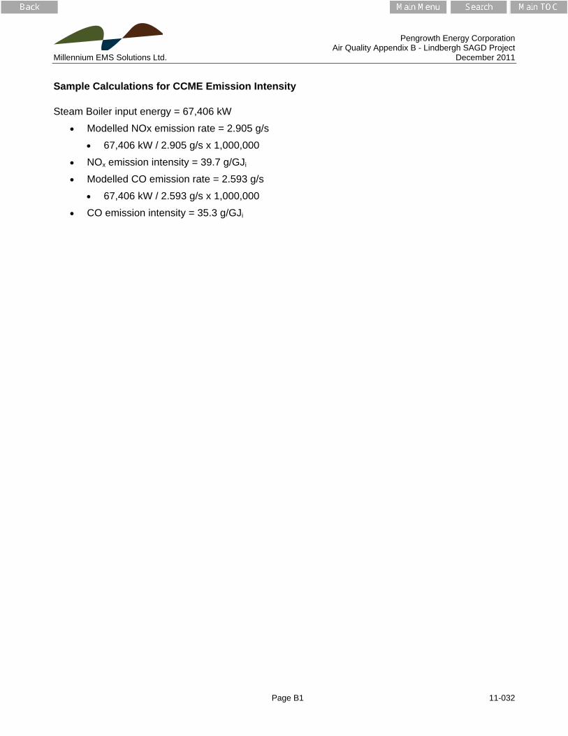
Pengrowth Energy Corporation Air Quality Appendix B - Lindbergh SAGD Project Millennium EMS Solutions Ltd. December 2011
Page B1 11-032
Sample Calculations for CCME Emission Intensity
Steam Boiler input energy = 67,406 kW
Modelled NOx emission rate = 2.905 g/s
67,406 kW / 2.905 g/s x 1,000,000
NOx emission intensity = 39.7 g/GJi
Modelled CO emission rate = 2.593 g/s
67,406 kW / 2.593 g/s x 1,000,000
CO emission intensity = 35.3 g/GJi