aircraft vehicle systems modeling and simulation under ...415979/fulltext01.pdf · aircraft vehicle...
TRANSCRIPT
L I N K Ö P I N G S T U D I E S I N S C I E N C E A N D T E C H N O L O G Y
T H E S I S N O 1 4 9 7
Aircraft Vehicle Systems Modeling and Simulation under Uncertainty
Sören Steinkellner
D E P A R T M E N T O F M A N A G E M E N T A N D E N G I N E E R I N G
D I V I S I O N O F M A C H I N E D E S I G N L I N K Ö P I N G S U N I V E R S I T E T
S E - 5 8 1 8 3 L I N K Ö P I N G
S W E D E N
L I N K Ö P I N G 2 0 1 1

ii
ISBN: 978-91-7393-136-6 ISSN: 0280-7971 LIU-TEK-LIC-2011:36 Copyright © June 2011 by Sören Steinkellner Distributed by: Linköpings universitet Department of Management and Engineering SE-581 83 Linköping, Sweden Tel: +46 13 281000, fax: +46 13 281873 Cover: Inspired by ”La trahison des images” (The Treachery of Images), René Magritte Printed in Sweden by LiU-Tryck Linköping, 2011
iii
Abstract
N AIRCRAFT DEVELOPMENT, it is crucial to understand and evaluate behavior, performance, safety and other aspects of the systems before and after they are physically
available for testing. Simulation models are used to gain knowledge in order to make decisions at all development stages.
Modeling and simulation (M&S) in aircraft system development, for example of fuel, hydraulic and electrical power systems, is today an important part of the design process. Through M&S a problem in a function or system is found early on in the process.
An increasing part of the end system verification relies on results from simulation models rather than expensive testing in flight tests. Consequently, the need for integrated models of complex systems, and their validation, is increasing. Not only one model is needed, but several interacting models with known accuracies and validity ranges are required. The development of computer performance and modeling and simulation tools has enabled large-scale simulation.
This thesis includes four papers related to these topics. The first paper describes a modeling technique, hosted simulation, how to simulate a complete system with models from different tools, e.g. control software from one tool and the equipment model from another. The second paper describes the use of M&S in the development of an aircraft. The third and fourth papers describe how to increase knowledge of the model’s validity by sensitivity analysis and the uncertainty sources.
In papers one and three an unmanned aerial vehicle is used as an example and in paper four a pressure regulator is the application.
I

iv
v
Acknowledgements
HE WORK PRESENTED in this thesis has been carried out at the Division of Machine Design at the Department of Management and Engineering (IEI) at Linköping University,
Sweden. I am very grateful to all the people who have supported me during the work with this thesis. First of all I would like to thank my supervisor and examiner Prof. Petter Krus for all his help with and input to the thesis. I would also like to thank my project leaders for taking care of all contractual and financial issues; the first project leader, Dr. Birgitta Lantto, who initiated the project and had patience with all the initial delays, and the second project leader, Dr. Ingela Lind, who finished it all. Then I would like to thank my speaking-partner and co-author of some of my papers Tekn. Lic. Henric Anderson, whom without my doctoral studies would not have been as interesting, fun and rewarding. I would also like to thank my remaining co-authors, Dr. Hampus Gavel, Dr. Ingela Lind, and Prof. Petter Krus. Moreover I would like to thank Dr. Olof Johansson and Prof. Johan Ölvander for reviewing, the two master thesis students Emil Larsson and Ylva Jung for their contributions, and my opponent Dr. Björn Lundén.
Finally, I am very grateful to my wife Siw for her support and encouragement and my son Matteo for his patience.
The research environment at the Division of Machine Design and its close neighbor Fluid and Mechatronic Systems was characterized by stimulating and generous colleagues.
This research work was funded by the Swedish National Aviation Engineering Research Programme (NFFP) and Saab Research Council in close relationship with the EC project CRESCENDO (Collaborative and Robust Engineering using Simulation Capability Enabling Next Design Optimisation). Linköping, June 2011
Sören Steinkellner
T

vi
vii
Nomenclature
Abbreviations
a/c Aircraft APESS Auxiliary power system ATA Air Transport Association CFD Computational Fluid Dynamics DAE Differential Algebraic Equation DDE Dynamic Data Exchange ECS Environmental Control System EIM Effective Influence Matrix ECU Electronic Control Unit FMI Functional Mockup Interface FS Fuel System GUI Graphical User Interface HILS Hardware In-the-Loop Simulation HMI Human Man Interface HS Hosted Simulation HSS Hydraulic Supply System INCOSE The International Council on Systems Engineering M&S Modeling and Simulation MBD Model Based Design MBD Model Based Development MBD Model Based Definition MBE Model Based Engineering MBSE Model Based Systems Engineering MDA Model Driven Architecture MDD Model Driven Design MDE Model Driven Engineering MSI Main Sensitivity Index ODE Ordinary Differential Equation PDE Partial Differential Equation

viii
S-ECS Secondary environmental control system SA Sensitivity analysis SE Systems Engineering TSI Total Sensitivity Index UAV Unmanned Aerial Vehicle V&V Verification and Validation VBA Visual Basic for Applications
ix
Papers
HIS THESIS IS based on the following four appended papers, which will be referred to by their Roman numerals. The papers are printed in their originally published state except for
changes in formatting and correction of minor errata. [I] Steinkellner S., Andersson H., Krus P., Lind I., “Hosted Simulation for Heterogeneous
Aircraft System Development”, 26th International Congress of the Aeronautical Sciences, Anchorage, Alaska, ICAS2008-6.2 ST, 2008.
[II] Steinkellner S., Andersson H., Gavel H., Krus P., ”Modeling and simulation of Saab
Gripen’s vehicle systems”, AIAA Modeling and Simulation Technologies Conference, AIAA 2009-6134, Chicago, USA, 2009.
[III] Steinkellner S., Krus P., ”Balancing Uncertainties in Aircraft System Simulation Models”
2nd European Air & Space Conference CEAS, Manchester, United Kingdom, 2009. [IV] Steinkellner S., Andersson H., Gavel H., Lind I., Krus P., “Modeling and simulation of
Saab Gripens vehicle systems, challenges in process and data uncertainties” 27th International Congress of the Aeronautical Sciences, Nice, France, ICAS2010-7.3.1, 2010.
T
x
The following papers are not appended to this thesis but constitute a part of the background. [V] Ellström H., Steinkellner S., “Modelling of pressurized fuel systems in military aircrafts,”
Proceedings of Simulation of Onboard systems, Royal Aeronautical Society, London, 2004.
[VI] Gavel H., Lantto B., Ellström H., Jareland M., Steinkellner S., Krus P., Andersson J.,
“Strategy for Modeling of large A/C fluid systems”, SAE Transactions Journal of Aerospace 2004, pp 1495-1506, 2004.
[VII] Lantto B., Ellström H., Gavel H., Jareland M., Steinkellner S., Järlestål A., Landberg M.,
“Modeling and Simulation of Gripen’s Fluid Power Systems” Recent advances in aerospace actuation systems and components, Toulouse, France, 2004.
[VIII] Andersson H., Steinkellner S., Erlandsson H., Krus P., “Configuration management of
models for aircraft simulation” 27th International Congress of the Aeronautical Sciences, Nice, France, ICAS2010-7.9.2, 2010.
xi
Contents
1 INTRODUCTION.......................................................................................................................... 1
1.1 AIM, LIMITATION AND CONTEXT ............................................................................................. 2 1.2 RESEARCH METHOD................................................................................................................. 3 1.3 THESIS OUTLINE ...................................................................................................................... 4
2 FRAME OF REFERENCE........................................................................................................... 5
2.1 MODELS .................................................................................................................................. 5 2.2 SIMULATION OF MATHEMATICAL MODELS............................................................................... 7 2.3 MODELING AND SIMULATION TOOLS ....................................................................................... 9 2.4 MODELING AND SIMULATION HISTORY...................................................................................11 2.5 MODEL BASED SYSTEMS ENGINEERING ..................................................................................11 2.6 THE MODEL BASED DESIGN PROCESS ......................................................................................12 2.7 AIRCRAFT SUBSYSTEMS .........................................................................................................13 2.8 AIRCRAFT SYSTEM SIMULATION AND SIMULATORS ................................................................15 2.9 VERIFICATION AND VALIDATION ............................................................................................15
3 MODELING AND SIMULATION OF VEHICLE SYSTEMS ................................................17
3.1 BACKGROUND ........................................................................................................................17 3.2 THE GRIPEN VEHICLE SYSTEM MODELS ..................................................................................18 3.3 HOSTED SIMULATION OF HETEROGENEOUS MODELS...............................................................20
3.3.1. Modeling techniques ....................................................................................................21 3.3.2. Equipment model..........................................................................................................22 3.3.3. Complete control code model.......................................................................................23 3.3.4. Model implementation. Signal-flow tool as host ..........................................................23 3.3.5. Model implementation. Power-port tool as host ..........................................................24 3.3.6. Hosted simulation experiences.....................................................................................24
3.4 THE GRIPEN’S VEHICLE SYSTEM DEVELOPMENT ....................................................................24
4 SENSITIVITY ANALYSIS AND PROCESSES ........................................................................27
4.1 MODELING AND SIMULATION PROCESS...................................................................................27 4.2 SENSITIVITY ANALYSIS...........................................................................................................30
4.2.1. Sensitivity analysis process ..........................................................................................31 4.2.2. Sensitivity analysis in the vehicle system design process .............................................31
4.3 UNCERTAINTIES .....................................................................................................................32 4.3.1. Parameter uncertainties...............................................................................................32 4.3.2. Model structure uncertainties ......................................................................................33 4.3.3. Model validation data uncertainties ............................................................................33 4.3.4. Numerical simulation error..........................................................................................34 4.3.5. Model inputs.................................................................................................................34
xii
4.4 SENSITIVITY ANALYSIS MEASURES .........................................................................................36 4.5 UAV FUEL SYSTEM EXAMPLE.................................................................................................36
4.5.1. Local sensitivity analysis implementation....................................................................36 4.5.2. Local sensitivity analysis simulation............................................................................38
4.6 SUMMARY ..............................................................................................................................40
5 DISCUSSION AND CONCLUSIONS.........................................................................................41
5.1 REUSE OF MODELS..................................................................................................................42 5.2 TOOL CHAIN ...........................................................................................................................44 5.3 VALIDATION...........................................................................................................................45 5.4 SENSITIVITY ANALYSIS ..........................................................................................................45 5.5 ADEQUATE MODEL EQUATION LEVEL REPRESENTATION.........................................................46 5.6 SUMMARY ..............................................................................................................................47 5.7 FUTURE WORK........................................................................................................................48
6 REFERENCES..............................................................................................................................49
APPENDED PAPERS
[I] Hosted Simulation for Heterogeneous Aircraft System Development....................................................53 [II] Modeling and simulation of Saab Gripen’s vehicle systems...................................................................67 [III] Balancing Uncertainties in Aircraft System Simulation Models.............................................................85 [IV] Modeling and simulation of Saab Gripens vehicle systems,
challenges in process and data uncertainties.........................................................................................101
1
Introduction
VERYTHING THAT IS a representation of something is a model. Neelamkavil [56], is very illustrative. “A model is a simplified representation of a system intended to enhance our
ability to understand, predict and possibly control the behavior of the system.” By using a model many benefits can be made. Within development of complex products it has become common to use models of the product. In aircraft development, it is crucial to understand and evaluate behavior, performance, safety and other aspects of systems before and after they are physically available for testing. Simulation models are used to gain knowledge in order to make decisions at all development stages. Use of models increases the product’s maturity. Early detection and correction of design faults cost 200-1,000 times less than at later stages, [5]. This realization has led to an increase in modeling and simulation (M&S) activity in early development phases. Another reason is the relationship between market requests for products with high functionality, which often results in complex system interactions that M&S can describe/develop. Added to this is also the financial incentive to minimize product development time and cost which M&S supports.
The activity “model validation” is difficult to perform in early development phases such as the concept phase due to the need for comparable system experiment data. This complicates the current design process that originates from the days of fewer early M&S activities and later M&S activities with models validated by experiments. Methods to increase and quantify the reliability of the model before access to measurement data are lagging behind the use of models and must be improved and used to achieve a credible development environment.
There exist many model uncertainty sources that are the reasons for the models’ unknown validity. Some of the main sources are, paper [IV]:
• model parameter uncertainties • model structure uncertainties • model validation data uncertainties • model input uncertainties
The use of M&S in early system development phases has increased. This has led to the emerging need for uncertainty management and more complete validation methods that complement the traditional validation based on measurement data, knowledge of a model’s maturity, and
E
2 Aircraft Vehicle Systems Modeling and Simulation under uncertainty
simulation result accuracy. A solution to this need is important to succeed in system development where early design decisions have to be made supported by simulation.
Sensitivity analyses can be made to point out model parameters/inputs that have a strong influence on the simulation result or compare the assumed uncertainty data influence with similar model accuracy experience. Sensitivity analyses can therefore support the process of increasing knowledge of the models’ validity.
The ability to handle uncertain information and lack of information is the key to success in early design.
1.1 Aim, limitation and context
The aim of the research is to provide industrially useful methods for supporting model validation when measurement data is lacking. First, simulation techniques are needed that enable system simulation with models from different domains, paper [I]. Second, as a model constantly evolves through the development process, these validation methods must also fit into the entire development process, paper [II]. Third, the industrial applicability of the methods and metrics using uncertainty data must be investigated, paper [III]. Finally, the sources of uncertainty must be identified and classified to be able to take an effective countermeasure to ensure that the model output can be a base for decision, paper [IV].
One limitation that reduces the number of methods is that the selected model category, mathematically based aircraft vehicle system models, is computationally demanding. Others are that the model equations are not explicitly accessible and that the number of model parameters affected by uncertainty can be relatively large.
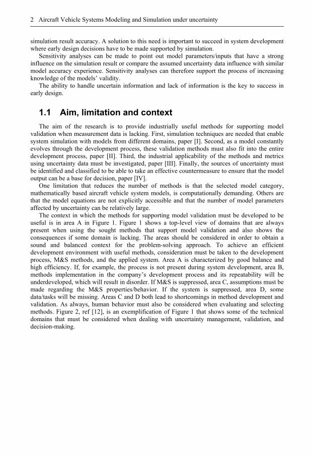
The context in which the methods for supporting model validation must be developed to be useful is in area A in Figure 1. Figure 1 shows a top-level view of domains that are always present when using the sought methods that support model validation and also shows the consequences if some domain is lacking. The areas should be considered in order to obtain a sound and balanced context for the problem-solving approach. To achieve an efficient development environment with useful methods, consideration must be taken to the development process, M&S methods, and the applied system. Area A is characterized by good balance and high efficiency. If, for example, the process is not present during system development, area B, methods implementation in the company’s development process and its repeatability will be underdeveloped, which will result in disorder. If M&S is suppressed, area C, assumptions must be made regarding the M&S properties/behavior. If the system is suppressed, area D, some data/tasks will be missing. Areas C and D both lead to shortcomings in method development and validation. As always, human behavior must also be considered when evaluating and selecting methods. Figure 2, ref [12], is an exemplification of Figure 1 that shows some of the technical domains that must be considered when dealing with uncertainty management, validation, and decision-making.
Introduction 3
System development characterized byA: Efficiency B: Disorder C: AssumptionsD: Absence of data/tasks
ABC
D
System
Process M&S
Figure 1 A top-level view of domains that should be considered in order to obtain a sound, balanced context for the problem-solving approach.
Project management
Risk management
System engineering
Simulation engineering
Knowledge engineering
Software engineering
Test engineering
Quality management
Metrology
Decision making
Uncertainty management
Verification, validation & acceptance
Figure 2 Uncertainty management, validation, and decision-making are closely connected and have an inherently complex relationship between technical domains, ref [12]. It is the author’s opinion that the figure can be improved by adding a technical system specialist to the original domains.
1.2 Research method
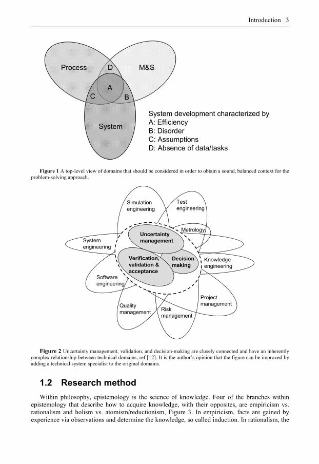
Within philosophy, epistemology is the science of knowledge. Four of the branches within epistemology that describe how to acquire knowledge, with their opposites, are empiricism vs. rationalism and holism vs. atomism/reductionism, Figure 3. In empiricism, facts are gained by experience via observations and determine the knowledge, so called induction. In rationalism, the
4 Aircraft Vehicle Systems Modeling and Simulation under uncertainty
intellectual can draw conclusions without any observations, so called deduction. Holism is an approach in which the whole is greater than the sum of its parts and that nothing can be described individually, without its context, compared to atomism/reductionism that endeavors to solve all problems by breaking them down into smaller parts and using these to explain and solve problems, ref [22].
This work is an industrial thesis where knowledge is acquired by experience and the research content is influenced by requirements and conditions that exist in a large organization that develops complex products, such as aircraft. The research method used is therefore best described as induction. A context breakdown is followed by a modeling and simulation phase that leads to methods proposal. The research method used is similar to the “Industry-as-laboratory” approach, [59] that has frequent exchanges of information between the problem domain (industry) and the academic domain.
Empiricism
Rationalism
HolismAtomism
Research specification
(Classical medicine research)
(Mathematical derivations)
(QualitativeMethods)
(Philosophicalresearch)
Context breakdown
Modeling
Simulation
Method proposal
Result validation
Figure 3 A simplified view of the different methodological principal axes that exist when it comes to producing
new knowledge with papers [I-IV], schematically drawn with their relationships. Adapted from [22].
1.3 Thesis outline
This thesis is divided into three main sections: • Chapter 2 Frame of reference. An introduction to M&S, model-based design, and
aircraft systems. • Chapter 3 Modeling and simulation of vehicle systems. An overview of how aircraft
vehicle systems are designed in an M&S context. One simulation technique, hosted simulation, is described in detail.
• Chapter 4 Sensitivity analysis and processes. The sensitivity analysis method is described together with how it fits into the M&S process. The different uncertainty data sources that are used in sensitivity analysis are described. The “local sensitivity analysis” technique and its measures are used on an unmanned aerial vehicle (UAV) fuel system.
Frame of reference 5
2 Frame of reference
HIS SECTION PROVIDES an overview of model classification, simulation methods and their relation to engineering and aircraft system classification. The focus is on mathematical
models for aircraft vehicle systems.
2.1 Models
Everything that is a representation of something can be seen as a model. In other words, a model is a simplification of something, e.g. anything from a screw to an airplane. Even non-technical areas can be modeled as living organisms, abstract social behavior, and economic progress. A model represents a system. A general definition of a system is given by [16].
“The largest possible system of all is the universe. Whenever we decide to cut out a piece of the universe such that we can clearly say what is inside that piece (belongs to that piece), and what is outside (does not belong to that piece), we define a new system. A system is characterized by the fact that we can say what belongs to it and what does not, and by the fact that we can specify how it interacts with its environment. System definitions can furthermore be hierarchical. We can take the piece from before, cut out a yet smaller part of it, and we have a new system.”
Examples of models related to a pump might be a thought or idea for its performance and type, a piece of plastic that shows its geometric extent, a blueprint, a textual description, mathematical equations that predict its performance, or a prototype. The model simplifies and helps the user to better understand the real object. Models can fall into at least four categories, [49] and [68] :
• Physical • Schematic • Verbal/Mental • Mathematical
Physical models attempt to recall the system in terms of appearance. Typical physical models are scale models used in e.g. wind tunnels, test rigs, mock-ups or prototypes. Note that the term ‘physical models’ is somewhat confusingly also used in the field of physics, for example for mathematical models.
T
6 Aircraft Vehicle Systems Modeling and Simulation under uncertainty
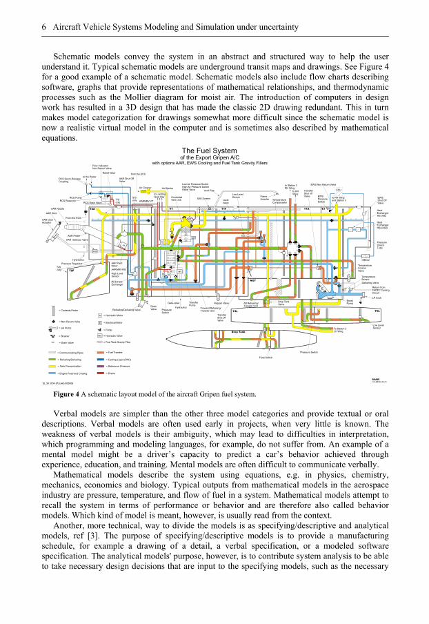
Schematic models convey the system in an abstract and structured way to help the user understand it. Typical schematic models are underground transit maps and drawings. See Figure 4 for a good example of a schematic model. Schematic models also include flow charts describing software, graphs that provide representations of mathematical relationships, and thermodynamic processes such as the Mollier diagram for moist air. The introduction of computers in design work has resulted in a 3D design that has made the classic 2D drawing redundant. This in turn makes model categorization for drawings somewhat more difficult since the schematic model is now a realistic virtual model in the computer and is sometimes also described by mathematical equations.
H
H
E
E
T/Sonly
S/Sonly
S/Sonly
The Fuel System
HV
HV
HV
HV
H
of the Export Gripen A/Cwith options AAR, EWS Cooling and Fuel Tank Gravity Fillers
J1-A-B6042-AA-01
RCS Quick-ReleaseCoupling
to the Radar
Flow Indicator/Non Return Valve
Relief Valve
RCS ReservoirRCS Drain Valve
RCS Pump
From the ECS
Hydraulics
AAR Door
AAR Nozzle
AAR DoorActuator
AAR Probe
AAR Selector Valve
T2F
T2A VT T1F T1A T3
NGT
T4L T5L
Drop Tank
AAR Shut OffValve
= Contents Probe
= Non Return Valve
= Jet Pump
= Strainer
= Drain Valve
= Hydraulic Motor
= Electrical Motor
= Pump
= Hydraulic Valve
= Fuel Tank Gravity Filler
RCS HeatExchanger
High LevelSensor
AARNRV-RG
AARNRV-VT
AAR Hydr.Motor
Pressure Regulator
PressureSwitch
Gate-valve
HydraulicsRefueling/Defueling Valve
DrainValve
TransferPump
Forward Refueling/Transfer Unit
Flapper Valve
Float Switch
Aft Refueling/Transfer Unit
To Station 3LH Wing
Drop TankValve
Pressure Switch
Low LevelSensor
BoostPump
Return fromFADEC CoolingCircuit
TemperatureSensorDefueling Valve
GECU
LP Cock
Transfer Shut offValve
TemperatureControlValve
PressureCheckTube
HeatExchangerHS1/MG
HeatExchangerHS2/AGB
FPU
EWSShut OffValve
EWSPressureSwitch
EWS Non Return Valve
TemperatureCompensator
FlameArrester
to Station 3RH Wing
to RH Wingand Station 3
To RH Wing
TransferShut offValve
Low LevelSensor
LevelValve
Vent Pipe
EMI Screen
Low Air Pressure SwitchHigh Air Pressure SwitchRelief Valve
ControlledVent Unit
Air EjectorAir Cleaner
to LandingGear Bay
from the ECS
= Communicating Pipes
= Refueling/Defueling
= Tank Pressurization
= Engine Feed and Cooling
= Fuel Transfer
= Cooling Liquid (PAO)
= Reference Pressure
= Drains
SL 39 3704 (P) (AA) 000609
Figure 4 A schematic layout model of the aircraft Gripen fuel system. Verbal models are simpler than the other three model categories and provide textual or oral
descriptions. Verbal models are often used early in projects, when very little is known. The weakness of verbal models is their ambiguity, which may lead to difficulties in interpretation, which programming and modeling languages, for example, do not suffer from. An example of a mental model might be a driver’s capacity to predict a car’s behavior achieved through experience, education, and training. Mental models are often difficult to communicate verbally.
Mathematical models describe the system using equations, e.g. in physics, chemistry, mechanics, economics and biology. Typical outputs from mathematical models in the aerospace industry are pressure, temperature, and flow of fuel in a system. Mathematical models attempt to recall the system in terms of performance or behavior and are therefore also called behavior models. Which kind of model is meant, however, is usually read from the context.
Another, more technical, way to divide the models is as specifying/descriptive and analytical models, ref [3]. The purpose of specifying/descriptive models is to provide a manufacturing schedule, for example a drawing of a detail, a verbal specification, or a modeled software specification. The analytical models' purpose, however, is to contribute system analysis to be able to take necessary design decisions that are input to the specifying models, such as the necessary
Frame of reference 7
performance and placement of a pump. The specifying models are usually used as a basis for analytical models, such as CFD models, and thus design iterations are necessary. If much of the design occurs in the analytical models, such as the selection and evaluation of system concepts, the analytical model corresponding to the selected system can then be considered a specifying/descriptive model in terms of system layout. The specifying model may have different resolutions and still be useful from day one of its construction, while the analytical model must be complete and the weakest link determines its quality.
The benefits of modeling are several, such as [68]: • Models require users to organize and sometimes quantify information and, in the process,
often indicate areas where additional information is needed. • Models provide a systematic approach to problem-solving. • Models increase understanding of the problem. • Models require users to be very specific about objectives. • Models serve as a consistent tool for evaluation. • Models provide a standardized format for analyzing a problem.
Verbal modeling is thus the process of reproducing and establishing interrelationships between entities of a system in a model. It can be argued that modeling has an intrinsic value because of all the benefits models provide in an industrial development environment.
2.2 Simulation of mathematical models
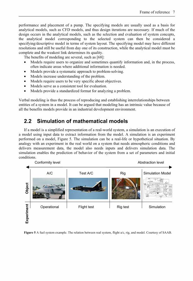
If a model is a simplified representation of a real-world system, a simulation is an execution of a model using input data to extract information from the model. A simulation is an experiment performed on a model, Figure 5. The simulation can be a real-life or hypothetical situation. By analogy with an experiment in the real world on a system that needs atmospheric conditions and delivers measurement data, the model also needs inputs and delivers simulation data. The simulation enables the prediction of behavior of the system from a set of parameters and initial conditions.
Test A/C Rig Simulation Model
Ob
jec
t
T2aftT3?T? T1aft
NGT
FRTU
Tp
ARTU
TpCVU
Ejector
RDT
CDT
LDT
sy?ambP?
RefuelRefuel
F
busT1busT2 busT3
busT45L
busT45R
busVT
busBPbusFRTU
busARTU
busCVU
FC
busGECU
busMission
Abstraction level
SimulationFlight test Rig test
Ex
per
ime
nt
Conformity level
A/C
Operational
Figure 5 A fuel system example. The relation between real system, flight a/c, rig, and model. Courtesy of SAAB.
8 Aircraft Vehicle Systems Modeling and Simulation under uncertainty
There are many reasons to simulate instead of setting up an experiment on a system in the real world [15]. The three main reasons are:
• It is too expensive to perform experiments on real systems, e.g. extensive drop tank separation analysis.
• It is too dangerous. The pilot can practice a dangerous maneuver before performing it in the plane.
• The system may not yet exist, i.e. the model will act as prototype that is evaluated and tested.
Other positive features that simulation provide are: • Variables not accessible in the real system can be observed in a simulation. • It is easy to use and modify models and to change parameters and perform new
simulations. With system design optimization many variants can be evaluated. • The time scale of the system may be extended or shortened. For example, a pressure peak
can be observed in detail or a flight of several hours can be simulated in minutes. The most important data flows in a model during simulation are:
• Parameters are constant during a simulation but can be changed in-between. • Constants are not accessible for the simulation user. • Variables are quantities that can vary with time. • Inputs are variables that affect the model. • For DAE/ODE/PDE models, states are an internal variable whose time derivative appears
in the model and must therefore be initialized at simulation start. • Outputs are variables that are observed.
The definitions of the terms vary depending on the domain. A promising standard, Functional Mockup Interface (FMI), has recently been developed, which can lead to a term alignment and simplified model integration between different technology domains and tools [24].
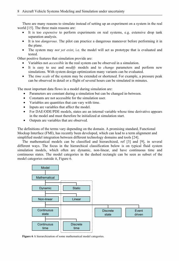
The mathematical models can be classified and hierarchized, ref [3] and [9], in several different ways. The focus in the hierarchical classification below is on typical fluid system simulation models, which often are dynamic, non-linear, and have continuous time and continuous states. The model categories in the dashed rectangle can be seen as subset of the model categories outside it, Figure 6.
Model
Mathematical
StaticDynamic
LinearNon-linear
Discretestate
Continuous state
Discrete time
Continuoustime
Eventdriven
Figure 6 A hierarchization of some mathematical model categories.
Frame of reference 9
In contrast to a static model, the output of a dynamic model can also be a function of the history of the models’ inputs and not only a function of the current inputs. For example, the pressure in the aircraft fuel tank is a function of previous flight conditions. The pressure will be different if the aircraft is climbing, diving, or in level flight just before the observed time. Dynamic models are typically represented with differential equations. Setting the time derivative of the states to zero in a dynamic model will result in a static model.
Strictly speaking, there are only non-linear systems in the real world but many systems are often modeled by linear models to simplify the M&S. Mathematical models describing fluid system are rarely linear. Non-linear models can be linearized in a working point for further analysis as if it were a linear model.
Sampling of an analog signal corresponds to a conversion of “Continuous time” to “Discrete time”.
Some other simulation output classifications are: • Deterministic vs. probabilistic models. The simulation output of a deterministic model
with a distinct set of input, model parameters, and model initialization will not differ from one simulation to another. Probabilistic models also include the probability distribution of the models’ inputs and parameters. Extensive simulation of such models will result in the outputs of the model being given a probability distribution. Typical uncertain parameters are fluid properties and equipment performance degradation due to wear/aging. A good representation of the probability distribution of the inputs and parameters in the model reflects probable measurement data distribution from aircraft or rig.
• Quantitative vs. qualitative models. A mathematical model of an aircraft system is a quantitative model. A qualitative model could be a definition of quality criteria, ref [38], for a mathematical model for an aircraft system.
• Event-based (state machines). A heterogeneous model is a model that consists of more than one model category, for example from a fuel system model with a continuous time equipment model connected to a discrete time control model.
2.3 Modeling and simulation tools
This chapter describes some aspects of modeling and simulation tools. Computational design is a growing field whose development is coupled to the rapid improvement of computers performance and their computational capability. There is no clear definition of the term computational design and it is interpreted differently in different engineering domains due its broad implications. However, computational design methods are characterized by operating on computer models in different ways in order to extract information, ref [17].
Historically. has each technical domain has developed its own tools. This is a natural consequence of the requirements for a tool being just as high and specific to the product complexity in itself. This is in order to achieve an efficient development environment. The increased complexity of the designed systems has put higher requirements on the tool’s capability to resemble the system and still have a high level of abstraction in combination with a user-friendly graphical interface (GUI). Models easily become complex and unstructured without an appropriate tool. There are several modeling-and-simulation tools on the market today that have a GUI that gives a good overview of the model. These are most often of the drag-and-drop type; this makes the modeling tool easy to use, thus minimizing the number of errors, ref [17].
Causality is the property of cause and effect in the system and it is an important condition for the choice of modeling technique and tool. For information flow or models of sensors or an Electronic Control Unit (ECU), the system’s inputs and outputs decide the causality. For physical
10 Aircraft Vehicle Systems Modeling and Simulation under uncertainty
systems with energy and mass flows, the causality is a question of modeling techniques/tools. In non-causal (or acausal) models, the causality is not explicitly stated, so the simulation tool has to sort the equations from model to the simulation code. When creating a causal model of a typical energy intensive system, the modeler has to choose what is considered to be a component’s input and output. The bond graph modeling technique, ref [58], is a method that aids transformation from non-causal to causal models. The bond graph is an energy-based graphical technique for building mathematical models of dynamic systems.
Thus, there are basically two representations, the signal flow/port approach using block diagrams suited to causal parts of the system and the power port approach, suitable for the non-causal parts. The chosen approach should be based on the dominating causality characteristics of the system, but is sometimes an outcome of the tool available. The signal port approach clearly shows all variable couplings in the system. This is very useful for systems analysis and is therefore suitable for representing control systems and systems connected to them. However, a drawback is that the model may become complex and difficult to overview. In this case, power port modeling is more appropriate. In power port modeling, there are bi-directional nodes that contain the transfer of several variables. Power port is more compact and closely matches the real physical connection that by nature is bi-directional.
Two examples of tools/languages for aircraft system development are: • Modelica, ref [35], is an object-oriented language for modeling complex physical
systems. Modelica is suitable for multi-domain modeling, for example modeling of mechatronic systems within aerospace applications. Such systems are composed of mechanical, electrical, and hydraulic subsystems, as well as control systems. Modelica uses equation-based modeling; the physical behavior of a model is described by differential, algebraic and discrete equations. Modelica models are acausal and use the power port technique. An M&S environment is needed to solve actual problems. The environment provides a customizable set of block libraries that let users design and simulate. There are both commercial and free M&S environments for Modelica. Dymola, ref [25], OpenModelica, ref [37], and SimulationX, ref [28], are well known commercial Modelica tools.
• Simulink, ref [33], is also an environment for multi-domain M&S. Simulink is a product
from the tool vendor Mathworks. The biggest difference compared to Modelica tools is that the models will be causal and use the signal flow technique. A causal block diagram is made up of connected operation blocks. The connections stand for signals, which are propagated from one block to the next. Blocks can be purely algebraic or may involve some notion of time such as delay or integration. A product called Simscape, ref [32], has existed for some years that extends Simulink with tools for power port modeling of systems such as mechanical, electrical and, hydraulic.
Most simulation packages come with predefined libraries with sets of equations representing physical components. One of the major reasons for choosing a particular tool is whether a suitable component library already exists. Even so, it is not uncommon that some components may need to be tailored and added in order to simulate a specific system. When choosing a library, it is important to know to what levels of accuracy and bandwidth the components in the library are valid.
Frame of reference 11
2.4 Modeling and simulation history
This brief description of modeling and simulation history begins in the late 1970s as the availability of computers and computer-based calculation capacity began to increase for the engineers.
In the late 1970s, Schlesinger [63] defined the M&S activities, such as verification and validation and their relationship, and this has been improved upon by Sargent [61] with the real-world and simulation-world relationship with its analogies.
Before the 1980s, the modeling of larger vehicle system models was often error prone due to difficulties in visualizing and modifying the model.
In the 1980s, the era as we know it today began, with tools that have user-friendly graphical user interfaces with features like “drag and drop” of block components and the power port (based on bond graph technique) concept or at least appears to be power port to the user. Boeing's EASY5 is one such example of an early M&S tool.
In the 1990s, the co-simulation between tools became a common feature of commercial tools and heterogeneous simulation increased and the first version of the multi-domain modeling language Modelica was released [36] in 1997. The language has come to be used in both industry/academia and in different physical domains.
In the 2000s, it has become common to generate code from models directly to product or for hosted simulation, paper [I]. A new, mature and M&S-friendly design organization changed the complete fundamentals of the relationship of M&S and the design process. This change resulted in a new way of working, Model Based Systems Engineering (MBSE), with a model-centric development approach.
2.5 Model based systems engineering
The International Council on Systems Engineering (INCOSE) defines Systems Engineering (SE) as “Systems Engineering is an interdisciplinary approach and means to enable the realization of successful systems. It focuses on defining customer needs and required functionality early in the development cycle, documenting requirements, then proceeding with design synthesis and system validation while considering the complete problem, operations, cost & schedule, performance, training & support test, disposal and manufacturing”, ref [27].
SE with a model based approach is called MBSE. MBSE uses "modeling" of the system in, for example, the design of complex systems and of its requirements to facilitate a more efficient design process. There are several definitions of how models are used in system development depending on when in the design process it is used and in which technical domain, for example:
• MBSE (Model Based Systems Engineering) • MBD (Model Based Design) • MBD (Model Based Development) • MBD (Model Based Definition) • MBE (Model Based Engineering) • MDA (Model Driven Architecture) • MDD (Model Driven Design) • MDE (Model Driven Engineering)
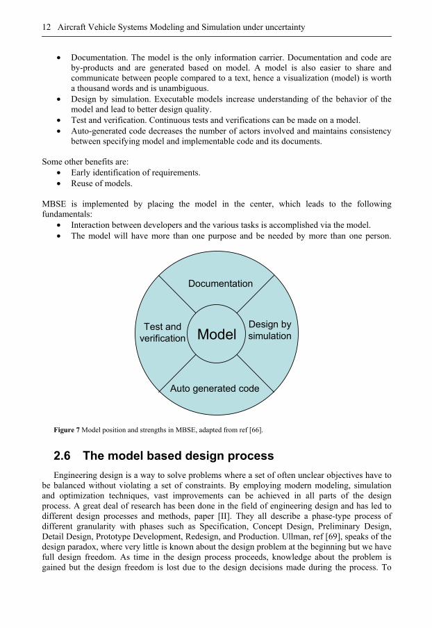
As M&S grows, the above definitions are exchanged between domains and are used in wider/slightly different senses. Some of the definitions are principles and some are the means to perform the principles, e.g. the principle of MBSE is used to perform MBD, ref [3]. Some of the major benefits, Figure 7, of a model-centric approach are:
12 Aircraft Vehicle Systems Modeling and Simulation under uncertainty
• Documentation. The model is the only information carrier. Documentation and code are by-products and are generated based on model. A model is also easier to share and communicate between people compared to a text, hence a visualization (model) is worth a thousand words and is unambiguous.
• Design by simulation. Executable models increase understanding of the behavior of the model and lead to better design quality.
• Test and verification. Continuous tests and verifications can be made on a model. • Auto-generated code decreases the number of actors involved and maintains consistency
between specifying model and implementable code and its documents.
Some other benefits are: • Early identification of requirements. • Reuse of models.
MBSE is implemented by placing the model in the center, which leads to the following fundamentals:
• Interaction between developers and the various tasks is accomplished via the model. • The model will have more than one purpose and be needed by more than one person.
Documentation
Model Design by simulation
Auto generated code
Test and verification
Figure 7 Model position and strengths in MBSE, adapted from ref [66].
2.6 The model based design process
Engineering design is a way to solve problems where a set of often unclear objectives have to be balanced without violating a set of constraints. By employing modern modeling, simulation and optimization techniques, vast improvements can be achieved in all parts of the design process. A great deal of research has been done in the field of engineering design and has led to different design processes and methods, paper [II]. They all describe a phase-type process of different granularity with phases such as Specification, Concept Design, Preliminary Design, Detail Design, Prototype Development, Redesign, and Production. Ullman, ref [69], speaks of the design paradox, where very little is known about the design problem at the beginning but we have full design freedom. As time in the design process proceeds, knowledge about the problem is gained but the design freedom is lost due to the design decisions made during the process. To
Frame of reference 13
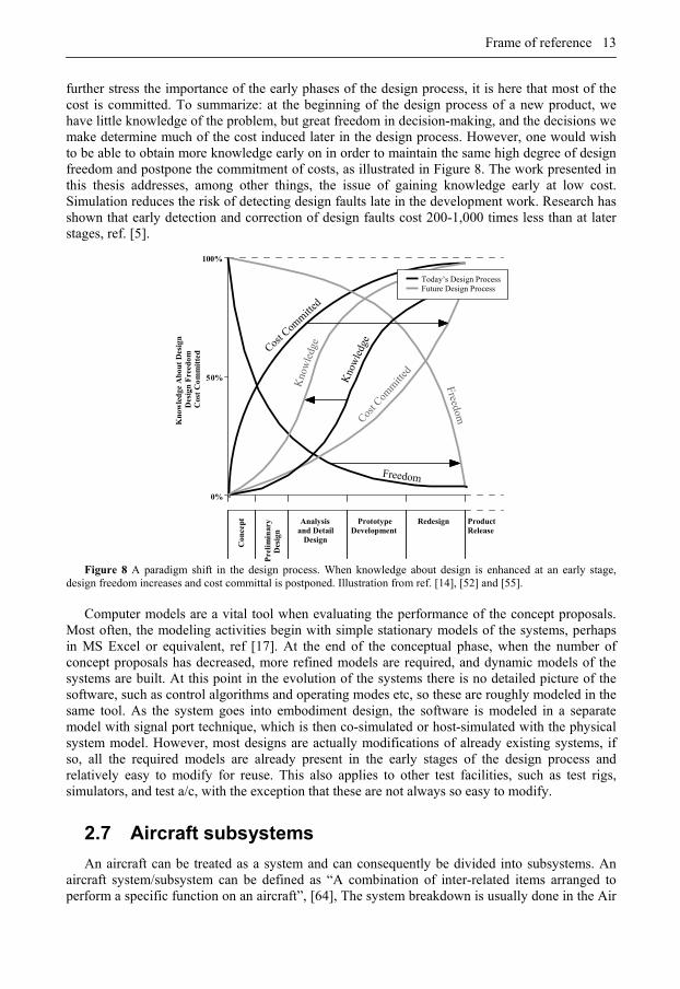
further stress the importance of the early phases of the design process, it is here that most of the cost is committed. To summarize: at the beginning of the design process of a new product, we have little knowledge of the problem, but great freedom in decision-making, and the decisions we make determine much of the cost induced later in the design process. However, one would wish to be able to obtain more knowledge early on in order to maintain the same high degree of design freedom and postpone the commitment of costs, as illustrated in Figure 8. The work presented in this thesis addresses, among other things, the issue of gaining knowledge early at low cost. Simulation reduces the risk of detecting design faults late in the development work. Research has shown that early detection and correction of design faults cost 200-1,000 times less than at later stages, ref. [5].
Cost C
ommitt
ed
Cost C
omm
itted
Freedom
Freedom
Kno
wle
dge
Kno
wle
dge
100%
50%
0%
Today’s Design Process Future Design Process
Kno
wle
dge
Abo
ut
Des
ign
Des
ign
Fre
edom
C
ost
Com
mit
ted
Con
cept
Pre
lim
inar
y D
esig
n
Analysisand Detail
Design
PrototypeDevelopment
Redesign Product Release
Figure 8 A paradigm shift in the design process. When knowledge about design is enhanced at an early stage,
design freedom increases and cost committal is postponed. Illustration from ref. [14], [52] and [55]. Computer models are a vital tool when evaluating the performance of the concept proposals.
Most often, the modeling activities begin with simple stationary models of the systems, perhaps in MS Excel or equivalent, ref [17]. At the end of the conceptual phase, when the number of concept proposals has decreased, more refined models are required, and dynamic models of the systems are built. At this point in the evolution of the systems there is no detailed picture of the software, such as control algorithms and operating modes etc, so these are roughly modeled in the same tool. As the system goes into embodiment design, the software is modeled in a separate model with signal port technique, which is then co-simulated or host-simulated with the physical system model. However, most designs are actually modifications of already existing systems, if so, all the required models are already present in the early stages of the design process and relatively easy to modify for reuse. This also applies to other test facilities, such as test rigs, simulators, and test a/c, with the exception that these are not always so easy to modify.
2.7 Aircraft subsystems
An aircraft can be treated as a system and can consequently be divided into subsystems. An aircraft system/subsystem can be defined as “A combination of inter-related items arranged to perform a specific function on an aircraft”, [64], The system breakdown is usually done in the Air
14 Aircraft Vehicle Systems Modeling and Simulation under uncertainty
Transport Association (ATA) chapter numbers, Table 1. The aircraft’s systems account for about 1/3 of a civil aircraft’s empty mass. More than 1/3 of the development and production costs of a medium-range civil aircraft can be allocated to the aircraft system and this ratio can even be higher for military aircrafts [64]. For example, for the Gripen the ratio for aircraft systems is 3/7 and a further 1/7 for associated system airframe installation, ref [2].
ATA Chapter name ATA Chapter name ATA SYSTEMS
ATA STRUCTURE
21 AIR CONDITIONING AND PRESSURIZATION 52 DOORS 22 AUTOFLIGHT 53 FUSELAGE 23 COMMUNICATIONS 54 NACELLES/PYLONS 24 ELECTRICAL POWER 55 STABILIZERS 25 EQUIPMENT/FURNISHINGS 56 WINDOWS 26 FIRE PROTECTION 57 WING 27 FLIGHT CONTROLS 28 FUEL 29 HYDRAULIC POWER 30 ICE AND RAIN PROTECTION POWER PLANT 31 INDICATING / RECORDING SYSTEM 71 POWER PLANT 32 LANDING GEAR 72 ENGINE 33 LIGHTS 73 ENGINE - FUEL AND CONTROL 34 NAVIGATION 74 IGNITION 35 OXYGEN 75 BLEED AIR 36 PNEUMATIC 76 ENGINE CONTROLS 37 VACUUM 38 WATER/WASTE 46 INFORMATION SYSTEMS 49 AIRBORNE AUXILIARY POWER
Table 1 Some ATA Numbers and chapter names.
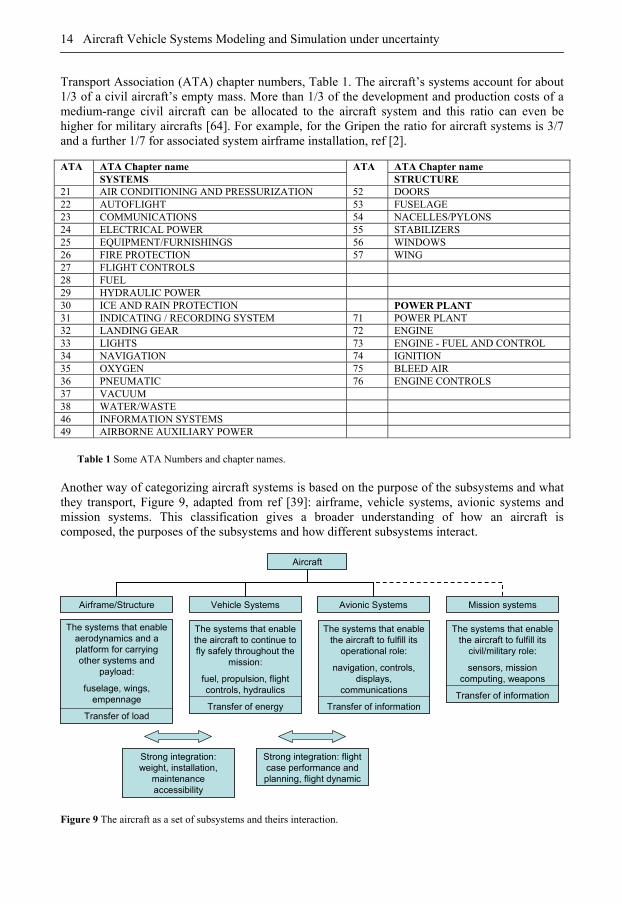
Another way of categorizing aircraft systems is based on the purpose of the subsystems and what they transport, Figure 9, adapted from ref [39]: airframe, vehicle systems, avionic systems and mission systems. This classification gives a broader understanding of how an aircraft is composed, the purposes of the subsystems and how different subsystems interact.
Aircraft
Vehicle Systems Avionic SystemsAirframe/Structure
The systems that enable aerodynamics and a platform for carrying other systems and
payload:
fuselage, wings, empennage
Transfer of load
Mission systems
The systems that enable the aircraft to continue to fly safely throughout the
mission:
fuel, propulsion, flight controls, hydraulics
Transfer of energy
Strong integration: weight, installation,
maintenance accessibility
Strong integration: flight case performance and planning, flight dynamic
The systems that enable the aircraft to fulfill its
operational role:
navigation, controls, displays,
communications
Transfer of information
The systems that enable the aircraft to fulfill its
civil/military role:
sensors, mission computing, weapons
Transfer of information
Figure 9 The aircraft as a set of subsystems and theirs interaction.
Frame of reference 15
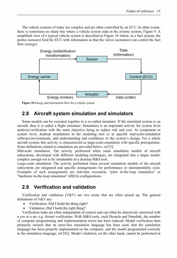
The vehicle systems of today are complex and are often controlled by an ECU. In other words,
there is sometimes no sharp line where a vehicle system ends in the avionic system, Figure 9. A simplified view of a typical vehicle system is described in Figure 10 where, in a fuel system, the probes (sensors) feed the ECU with information so that the valves (actuators) can control the fuel flow (energy).
Sensor
Control (ECU) Energy carrier
Actuator
Data (information)
Data (order)Energy (motion)
Energy (redistribution/transformation)
Figure 10 Energy and information flow for a vehicle system.
2.8 Aircraft system simulation and simulators
Some models can be executed together in a so-called simulator. If the simulated system is an aircraft, then it is called a flight simulator. Simulation is an important activity for system level analysis/verification with the main objective being to reduce risk and cost. At component or system level, desktop simulations in the modeling tool or in specific mid-scale-simulation software/environments, add understanding and confidence to the system’s design. For a whole aircraft system, this activity is characterized as large-scale-simulation with specific prerequisites. Some definitions related to simulation are provided below, ref [3]: Mid-scale simulation: The activity performed when some simulation models of aircraft subsystems, developed with different modeling techniques, are integrated into a larger model, complex enough not to be simulatable in a desktop M&S tool. Large-scale simulation: The activity performed when several simulation models of the aircraft subsystems are integrated and specific arrangements for performance or interoperability exist. Examples of such arrangements are real-time execution, “pilot in-the-loop simulation” or “hardware in-the-loop simulation” (HILS) configurations.
2.9 Verification and validation
Verification and validation (V&V) are two terms that are often mixed up. The general definitions of V&V are:
• Verification. Did I build the thing right? • Validation. Did I build the right thing?
Verification tasks are often independent of context and can often be objectively answered with a yes or a no, e.g. formal verification. With M&S tools, such Dymola and Simulink, the number of computer programming and implementation errors has been reduced. Model verification then primarily ensures that an error-free simulation language has been used, that the simulation language has been properly implemented on the computer, and the model programmed correctly in the simulation language, ref [62]. Model validation, on the other hand, cannot be performed in

16 Aircraft Vehicle Systems Modeling and Simulation under uncertainty
early development phases such as the concept phase due to the need for system experiment data. However, sensitivity analyses can still be made that point out model component parameters that have a strong influence on the simulation result or compare the assumed uncertainty data influence with similar model accuracy experience. Later in the development process, when more knowledge and measurement data is available, model validation with measurement data can begin. Model validation is context dependent, e.g. for a specific simulation task a model can be validated in parts of the flight envelope for some model outputs. For another simulation task with its context a complete other model validation status can exist.
In ref [38] a broader aspect and on a higher level has been taken concerning M&S result credibility. Eight factors have been defined with a five-level assessment of credibility for each factor, Verification Validation, Input Pedigree Results, Uncertainty, Results, Robustness, Use History M&S, Management, People, Qualifications. The approach clearly demonstrates the large number of factors that affect a model's credibility, which inevitably means that in the case of large models it is an extremely time-consuming task to make them credible.
Modeling and Simulation of Vehicle Systems 17
3
Modeling and
Simulation of Vehicle
Systems
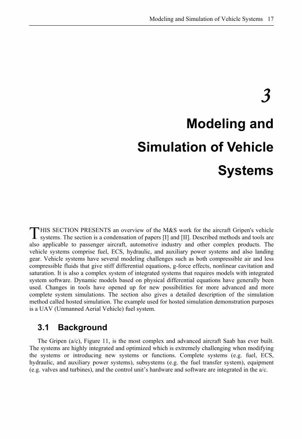
HIS SECTION PRESENTS an overview of the M&S work for the aircraft Gripen's vehicle systems. The section is a condensation of papers [I] and [II]. Described methods and tools are
also applicable to passenger aircraft, automotive industry and other complex products. The vehicle systems comprise fuel, ECS, hydraulic, and auxiliary power systems and also landing gear. Vehicle systems have several modeling challenges such as both compressible air and less compressible fluids that give stiff differential equations, g-force effects, nonlinear cavitation and saturation. It is also a complex system of integrated systems that requires models with integrated system software. Dynamic models based on physical differential equations have generally been used. Changes in tools have opened up for new possibilities for more advanced and more complete system simulations. The section also gives a detailed description of the simulation method called hosted simulation. The example used for hosted simulation demonstration purposes is a UAV (Unmanned Aerial Vehicle) fuel system.
3.1 Background
The Gripen (a/c), Figure 11, is the most complex and advanced aircraft Saab has ever built. The systems are highly integrated and optimized which is extremely challenging when modifying the systems or introducing new systems or functions. Complete systems (e.g. fuel, ECS, hydraulic, and auxiliary power systems), subsystems (e.g. the fuel transfer system), equipment (e.g. valves and turbines), and the control unit’s hardware and software are integrated in the a/c.
T
18 Aircraft Vehicle Systems Modeling and Simulation under uncertainty
Landing Gearand Braking Systems
Hydraulic System
Secondary Power System
Escape System
Electrical & Lighting Systems
Fuel SystemEnvironmentalControl System
Aircrew Equipment
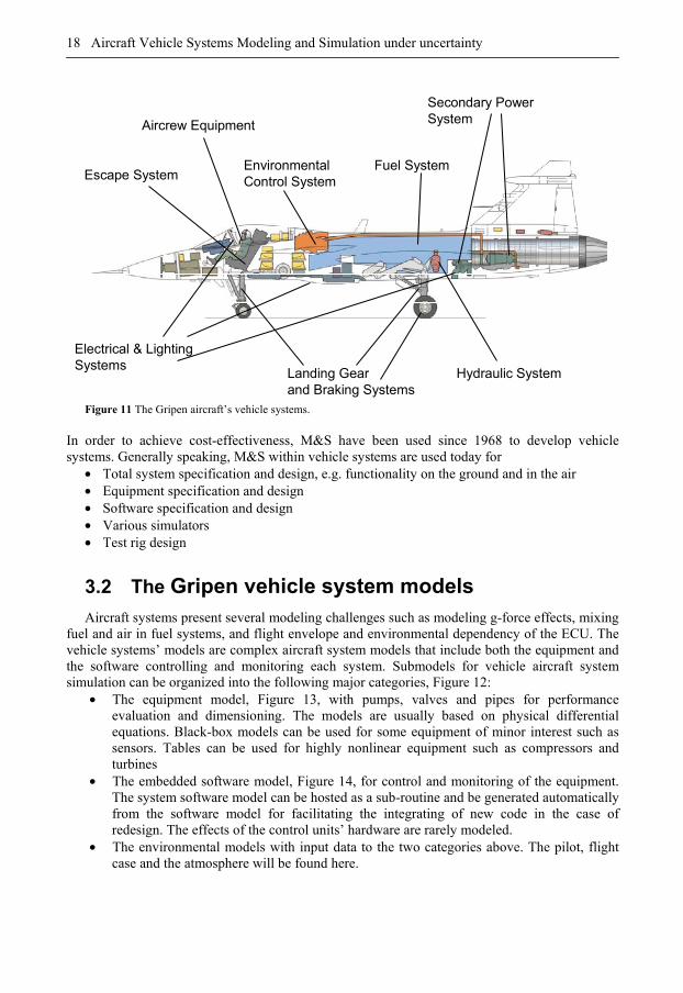
Figure 11 The Gripen aircraft’s vehicle systems.
In order to achieve cost-effectiveness, M&S have been used since 1968 to develop vehicle systems. Generally speaking, M&S within vehicle systems are used today for
• Total system specification and design, e.g. functionality on the ground and in the air • Equipment specification and design • Software specification and design • Various simulators • Test rig design
3.2 The Gripen vehicle system models
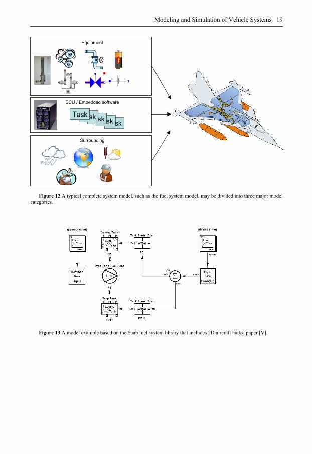
Aircraft systems present several modeling challenges such as modeling g-force effects, mixing fuel and air in fuel systems, and flight envelope and environmental dependency of the ECU. The vehicle systems’ models are complex aircraft system models that include both the equipment and the software controlling and monitoring each system. Submodels for vehicle aircraft system simulation can be organized into the following major categories, Figure 12:
• The equipment model, Figure 13, with pumps, valves and pipes for performance evaluation and dimensioning. The models are usually based on physical differential equations. Black-box models can be used for some equipment of minor interest such as sensors. Tables can be used for highly nonlinear equipment such as compressors and turbines
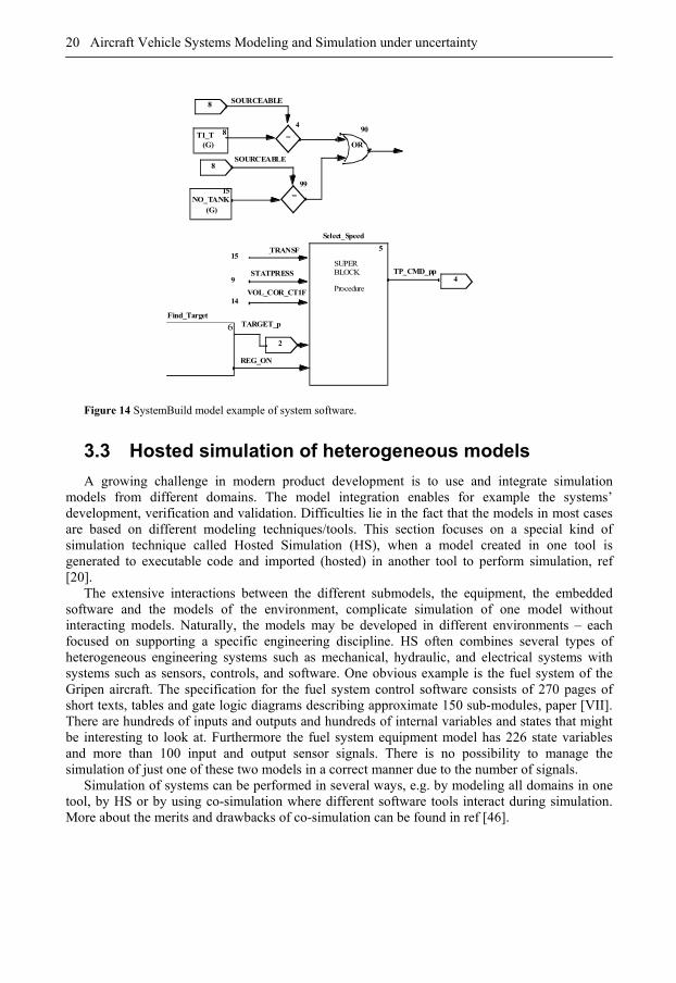
• The embedded software model, Figure 14, for control and monitoring of the equipment. The system software model can be hosted as a sub-routine and be generated automatically from the software model for facilitating the integrating of new code in the case of redesign. The effects of the control units’ hardware are rarely modeled.
• The environmental models with input data to the two categories above. The pilot, flight case and the atmosphere will be found here.
Modeling and Simulation of Vehicle Systems 19
TaskTaskTaskTaskTask
Equipment
ECU / Embedded software
Surrounding
Figure 12 A typical complete system model, such as the fuel system model, may be divided into three major model
categories.
Figure 13 A model example based on the Saab fuel system library that includes 2D aircraft tanks, paper [V].
20 Aircraft Vehicle Systems Modeling and Simulation under uncertainty
Figure 14 SystemBuild model example of system software.
3.3 Hosted simulation of heterogeneous models
A growing challenge in modern product development is to use and integrate simulation models from different domains. The model integration enables for example the systems’ development, verification and validation. Difficulties lie in the fact that the models in most cases are based on different modeling techniques/tools. This section focuses on a special kind of simulation technique called Hosted Simulation (HS), when a model created in one tool is generated to executable code and imported (hosted) in another tool to perform simulation, ref [20].
The extensive interactions between the different submodels, the equipment, the embedded software and the models of the environment, complicate simulation of one model without interacting models. Naturally, the models may be developed in different environments – each focused on supporting a specific engineering discipline. HS often combines several types of heterogeneous engineering systems such as mechanical, hydraulic, and electrical systems with systems such as sensors, controls, and software. One obvious example is the fuel system of the Gripen aircraft. The specification for the fuel system control software consists of 270 pages of short texts, tables and gate logic diagrams describing approximate 150 sub-modules, paper [VII]. There are hundreds of inputs and outputs and hundreds of internal variables and states that might be interesting to look at. Furthermore the fuel system equipment model has 226 state variables and more than 100 input and output sensor signals. There is no possibility to manage the simulation of just one of these two models in a correct manner due to the number of signals.
Simulation of systems can be performed in several ways, e.g. by modeling all domains in one tool, by HS or by using co-simulation where different software tools interact during simulation. More about the merits and drawbacks of co-simulation can be found in ref [46].
T1_T(G)
NO_TANK(G)
=
=
OR
SOURCEABLE
SOURCEABLE
8
15
8
8
=
4
99
BAD_TRANSF15
STATPRESS9
VOL_COR_CT1F14
TP_CMD_pp
5
Select_Speed
SUPERBLOCK
Procedure 4
90
6
REG_ON
Find_TargetTARGET_p
2
Modeling and Simulation of Vehicle Systems 21
3.3.1. Modeling techniques A challenging product development requires the most suitable tools in each engineering
domain. Several tools and techniques, ref [8] and [65], complicate the process of integrating models from different domains, for example a hybrid model containing the fuel system equipment and its control software.
A hybrid model is defined as combined discrete- and continuous-time parts, in which the continuous parts are based on differential equations, and the discrete parts are updated at event times. Typically, a continuous model is used to describe physical phenomena of the system equipment, whereas the discrete model is used to define software behavior, Figure 15. HS is powerful when combining these models, to close the loop, which gives a hybrid system model.
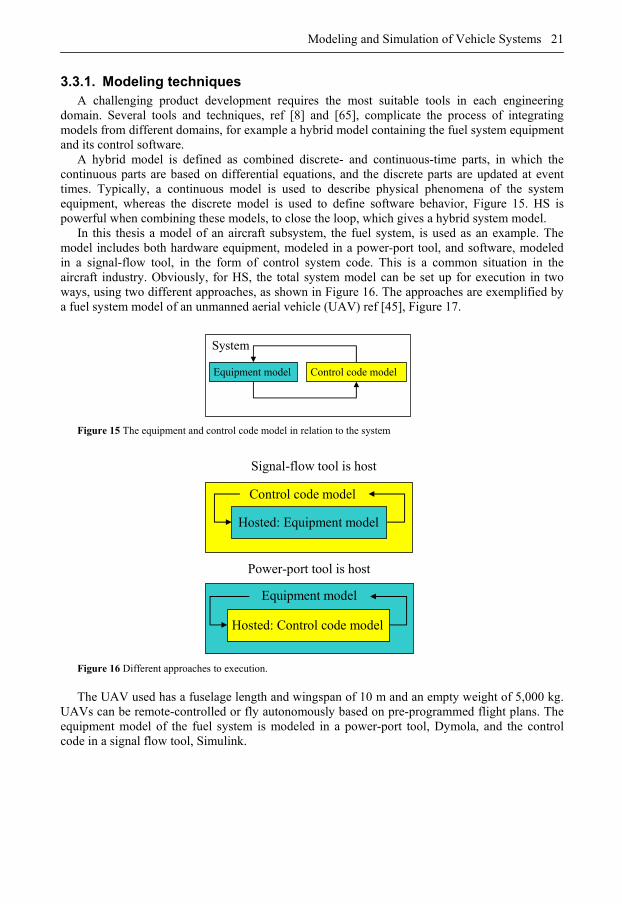
In this thesis a model of an aircraft subsystem, the fuel system, is used as an example. The model includes both hardware equipment, modeled in a power-port tool, and software, modeled in a signal-flow tool, in the form of control system code. This is a common situation in the aircraft industry. Obviously, for HS, the total system model can be set up for execution in two ways, using two different approaches, as shown in Figure 16. The approaches are exemplified by a fuel system model of an unmanned aerial vehicle (UAV) ref [45], Figure 17.
System
Equipment model Control code model
Figure 15 The equipment and control code model in relation to the system
Control code model
Equipment model
Signal-flow tool is host
Power-port tool is host
Hosted: Equipment model
Hosted: Control code model
Figure 16 Different approaches to execution.
The UAV used has a fuselage length and wingspan of 10 m and an empty weight of 5,000 kg.
UAVs can be remote-controlled or fly autonomously based on pre-programmed flight plans. The equipment model of the fuel system is modeled in a power-port tool, Dymola, and the control code in a signal flow tool, Simulink.
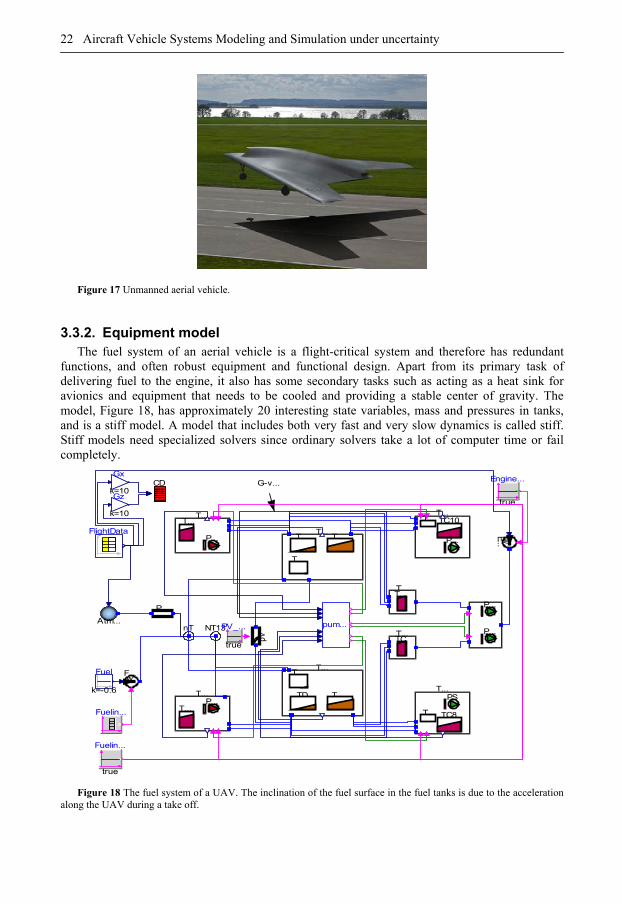
22 Aircraft Vehicle Systems Modeling and Simulation under uncertainty
Figure 17 Unmanned aerial vehicle.
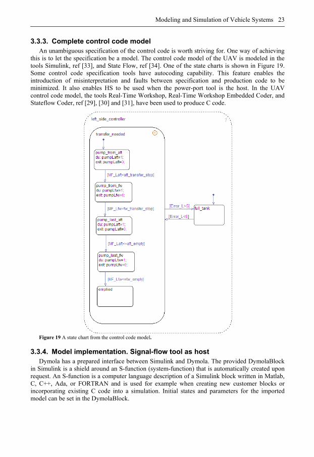
3.3.2. Equipment model The fuel system of an aerial vehicle is a flight-critical system and therefore has redundant
functions, and often robust equipment and functional design. Apart from its primary task of delivering fuel to the engine, it also has some secondary tasks such as acting as a heat sink for avionics and equipment that needs to be cooled and providing a stable center of gravity. The model, Figure 18, has approximately 20 interesting state variables, mass and pressures in tanks, and is a stiff model. A model that includes both very fast and very slow dynamics is called stiff. Stiff models need specialized solvers since ordinary solvers take a lot of computer time or fail completely.
T...T...
P...T...
T...
T... T...
T...T... TC10
P...
T...T...
T...
T...P...
T...T...
TD T...T...
T... TC8
PS
T...TC
P...
P...pum...
pV
nT NT13
P...
G-v...
Fuelin...
true
PV_...
true
Atm...
CD
FlightData
k=10
Gx
k=10
Gz
F...w
Fuel
k=-0.6
Fuelin...
E...w
Engine...
true
Figure 18 The fuel system of a UAV. The inclination of the fuel surface in the fuel tanks is due to the acceleration along the UAV during a take off.
Modeling and Simulation of Vehicle Systems 23
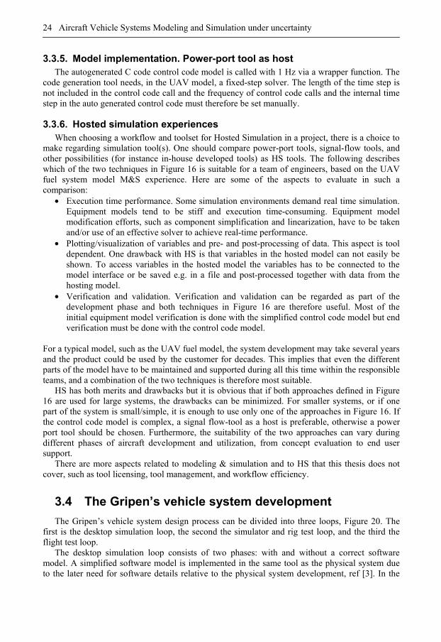
3.3.3. Complete control code model An unambiguous specification of the control code is worth striving for. One way of achieving
this is to let the specification be a model. The control code model of the UAV is modeled in the tools Simulink, ref [33], and State Flow, ref [34]. One of the state charts is shown in Figure 19. Some control code specification tools have autocoding capability. This feature enables the introduction of misinterpretation and faults between specification and production code to be minimized. It also enables HS to be used when the power-port tool is the host. In the UAV control code model, the tools Real-Time Workshop, Real-Time Workshop Embedded Coder, and Stateflow Coder, ref [29], [30] and [31], have been used to produce C code.
Figure 19 A state chart from the control code model.
3.3.4. Model implementation. Signal-flow tool as host Dymola has a prepared interface between Simulink and Dymola. The provided DymolaBlock
in Simulink is a shield around an S-function (system-function) that is automatically created upon request. An S-function is a computer language description of a Simulink block written in Matlab, C, C++, Ada, or FORTRAN and is used for example when creating new customer blocks or incorporating existing C code into a simulation. Initial states and parameters for the imported model can be set in the DymolaBlock.
24 Aircraft Vehicle Systems Modeling and Simulation under uncertainty
3.3.5. Model implementation. Power-port tool as host The autogenerated C code control code model is called with 1 Hz via a wrapper function. The
code generation tool needs, in the UAV model, a fixed-step solver. The length of the time step is not included in the control code call and the frequency of control code calls and the internal time step in the auto generated control code must therefore be set manually.
3.3.6. Hosted simulation experiences When choosing a workflow and toolset for Hosted Simulation in a project, there is a choice to
make regarding simulation tool(s). One should compare power-port tools, signal-flow tools, and other possibilities (for instance in-house developed tools) as HS tools. The following describes which of the two techniques in Figure 16 is suitable for a team of engineers, based on the UAV fuel system model M&S experience. Here are some of the aspects to evaluate in such a comparison:
• Execution time performance. Some simulation environments demand real time simulation. Equipment models tend to be stiff and execution time-consuming. Equipment model modification efforts, such as component simplification and linearization, have to be taken and/or use of an effective solver to achieve real-time performance.
• Plotting/visualization of variables and pre- and post-processing of data. This aspect is tool dependent. One drawback with HS is that variables in the hosted model can not easily be shown. To access variables in the hosted model the variables has to be connected to the model interface or be saved e.g. in a file and post-processed together with data from the hosting model.
• Verification and validation. Verification and validation can be regarded as part of the development phase and both techniques in Figure 16 are therefore useful. Most of the initial equipment model verification is done with the simplified control code model but end verification must be done with the control code model.
For a typical model, such as the UAV fuel model, the system development may take several years and the product could be used by the customer for decades. This implies that even the different parts of the model have to be maintained and supported during all this time within the responsible teams, and a combination of the two techniques is therefore most suitable.
HS has both merits and drawbacks but it is obvious that if both approaches defined in Figure 16 are used for large systems, the drawbacks can be minimized. For smaller systems, or if one part of the system is small/simple, it is enough to use only one of the approaches in Figure 16. If the control code model is complex, a signal flow-tool as a host is preferable, otherwise a power port tool should be chosen. Furthermore, the suitability of the two approaches can vary during different phases of aircraft development and utilization, from concept evaluation to end user support.
There are more aspects related to modeling & simulation and to HS that this thesis does not cover, such as tool licensing, tool management, and workflow efficiency.
3.4 The Gripen’s vehicle system development
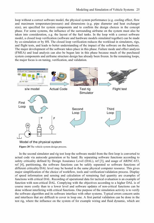
The Gripen’s vehicle system design process can be divided into three loops, Figure 20. The first is the desktop simulation loop, the second the simulator and rig test loop, and the third the flight test loop.
The desktop simulation loop consists of two phases: with and without a correct software model. A simplified software model is implemented in the same tool as the physical system due to the later need for software details relative to the physical system development, ref [3]. In the
Modeling and Simulation of Vehicle Systems 25
loop without a correct software model, the physical system performance (e.g. cooling effect, flow and maximum temperature/pressure) and dimensions (e.g. pipe diameter and heat exchanger size), are specified for system components and to confirm the design choices in the concept phase. For some systems, the influence of the surrounding airframe on the system must also be taken into consideration, e.g. the layout of the fuel tanks. In the loop with a correct software model, a closed loop verification (software and hardware models simulated together) can be made by co-simulation or by HS. The closed loop verification reduces the workload in simulators, rigs, and flight tests, and leads to better understanding of the impact of the software on the hardware. The major development of the software takes place in this phase. Failure mode and effect analysis (FMEA) and load analysis can also be begun late in this phase because much of the purchased system components and airframe structure design has already been frozen. In the remaining loops, the major focus is on tuning, verification, and validation.
Flight test
First Loop
SecondLoop
ThirdLoop
Model of the physical system
Actual Codes/w model
M
u y
M
u y
Test rigSimulator
Figure 20 The vehicle system design process. In the second simulator and rig test loop the software model from the first loop is converted to
actual code via autocode generation or by hand. By separating software functions according to safety criticality defined by Design Assurance Level (DAL), ref [3], and usage of ARINC-653, ref [4], partitioning, the software functions can be safely separated so software functions of different criticality/DAL level may be hosted in the same physical computer resource. This gives major simplification of the choice of workflow, tools and verification/validation process. Display of speed information and sensing and calculation of remaining fuel quantity are examples of functions with critical DAL. Recording of operational data for tactical evaluation is an example of function with non-critical DAL. Complying with the objectives according to a higher DAL is of course more costly than to a lower level and software updates of non-critical functions can be done without interfering with critical functions. One purpose of the simulation activity is to verify the software algorithm and its software interface with other systems. Typical errors concern units and interfaces that are difficult to cover in loop one. A first partial validation can be done in the test rig, where the influence on the system of for example wiring and fluid dynamic, which are
26 Aircraft Vehicle Systems Modeling and Simulation under uncertainty
seldom modeled, can be analyzed. To provide some degree of flexibility in the software, the concept of Flight Test Functions (FTF) is used; system software parameters have been listed in text files so that they can be changed without re-compiling the software. Typical activities performed in a rig are:
• Functional testing of hardware (fuel pump) • Performance test( pressure vs. flow of a fuel pump) • Functional testing of software • Static pressure data for static stress calculation • Dynamic pressure data for fatigue calculation • Fault location on equipment from aircraft • Data for model validation
An important part of the rig test activity is to feed the models with measurement data to improve the model’s accuracy.
If all modified software functions are non-critical in the flight test loop, flight tests are not considered mandatory. Some flight testing can perhaps nonetheless be conducted in parts of the flight envelope where the system model is not valid. If it is later shown in the aircraft that the software needs to be updated, this can be easily accomplished due to the separation from critical functions. If modified software functions are critical, flight tests are considered mandatory in order to secure airworthiness. The flight test should also provide the models with measurement data.
Sensitivity analysis and processes 27
4
Sensitivity analysis
and processes
HIS SECTION, WHICH IS a condensation of papers [III] and [IV], shows how the method sensitivity analysis fits and its usefulness at different stages of an M&S process. The example
used for demonstration purpose is a UAV fuel system.
4.1 Modeling and simulation process
The design process can be described in different ways. One way is represented by the process standard ISO 15288, which defines the engineering life cycle stages as concept, development, production, utilization, support and retirement. Aircraft subsystems are modeled and simulated intensively during the concept, development, utilization and support phases. Knowledge of the system increases during the engineering life cycle and models are continuously refined in order to respond to increasingly stricter requirements as regards the accuracy of the simulation results. A system model created at an early stage is often reused and further developed and refined in later design stages, Figure 21. A system simulation model is therefore not a static artifact that will be perfect or faultless despite it having been used and sometimes undergone several verification and validation phases.
The maturity of and confidence in a simulation model and the credibility of the simulation result increase continuously during its use, and are a logical consequence of the fact that a model cannot be fully validated, only corroborated to a greater degree, by using the model. In theory “… tests and evaluations are conducted until sufficient confidence is obtained that a model can be considered valid for its intended application” [61]. No general rule exists, so engineers must use their judgment as domain experts to decide whether additional testing is warranted [51], but in practice a model’s level of validity is often a consequence of project constraints such as time, money and human resources. Bearing in mind the fact that a model is not a static artifact, it is important that methods and model quality measures that support model improvements fit seamlessly into a company’s system development process, [6]. Otherwise, the strengths and
T
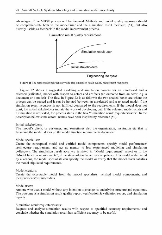
28 Aircraft Vehicle Systems Modeling and Simulation under uncertainty
advantages of the MBSE process will be lessened. Methods and model quality measures should be comprehensible both to the model user and the simulation result recipient, [51], but also directly usable as feedback in the model improvement process.
Simulation result quality requirement
Engineering life cycle
Initial stakeholders
Simulation result user
Figure 21 The relationship between early and late simulation result quality requirement requesters.
Figure 22 shows a suggested modeling and simulation process for an unreleased and a
released (validated) model with respect to actors and artifacts (an outcome from an actor, e.g. a document or a model). The flow in Figure 22 is as follows: the two shaded boxes are where the process can be started and it can be iterated between an unreleased and a released model if the simulation result accuracy is not fulfilled compared to the requirements. If the model does not exist, the initial stakeholders initiate the work of developing one. If the released model exists and a simulation is requested, the process starts in the box “Simulation result requesters/users”. In the description below some actors’ names have been inspired by reference [50].
Initial stakeholders: The model’s client, or customer, and sometimes also the organization, institution etc that is financing the model, draws up the model function requirements document. Model specialists: Create the conceptual model and verified model components, specify model performance/ architecture requirement, and act as mentor to less experienced modeling and simulation colleagues. The simulation result accuracy is stated in “Model requirement” report or in the “Model function requirements”, if the stakeholders have this competence. If a model is delivered by a vendor, the model specialists can specify the model or verify that the model reach satisfies the model stipulated requirements. Model creators: Create the executable model from the model specialists’ verified model components, and measurements/estimated data. Model users: Anyone who uses a model without any intention to change its underlying structure and equations. The outcome is a simulation result quality report, verification & validation report, and simulation reports. Simulation result requesters/users: Request and analyze simulation results with respect to specified accuracy requirements, and conclude whether the simulation result has sufficient accuracy to be useful.
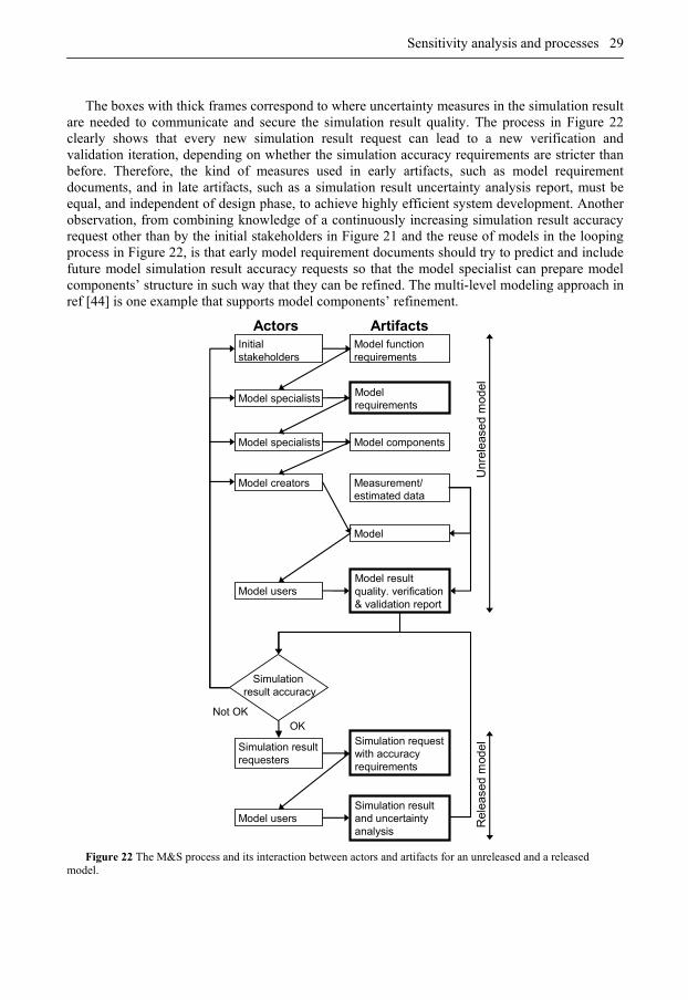
Sensitivity analysis and processes 29
The boxes with thick frames correspond to where uncertainty measures in the simulation result
are needed to communicate and secure the simulation result quality. The process in Figure 22 clearly shows that every new simulation result request can lead to a new verification and validation iteration, depending on whether the simulation accuracy requirements are stricter than before. Therefore, the kind of measures used in early artifacts, such as model requirement documents, and in late artifacts, such as a simulation result uncertainty analysis report, must be equal, and independent of design phase, to achieve highly efficient system development. Another observation, from combining knowledge of a continuously increasing simulation result accuracy request other than by the initial stakeholders in Figure 21 and the reuse of models in the looping process in Figure 22, is that early model requirement documents should try to predict and include future model simulation result accuracy requests so that the model specialist can prepare model components’ structure in such way that they can be refined. The multi-level modeling approach in ref [44] is one example that supports model components’ refinement.
Model function requirements
Initial stakeholders
Model requirements
Model specialists
Model componentsModel specialists
Model
Model creators Measurement/ estimated data
Model resultquality. verification& validation report
Model users
ArtifactsActors
Simulation request with accuracy requirements
Simulation result requesters
Model usersSimulation result and uncertainty analysis
OK
Simulationresult accuracy
Not OK
Unr
elea
sed
mo
del
Rel
ease
d m
ode
l
Figure 22 The M&S process and its interaction between actors and artifacts for an unreleased and a released
model.
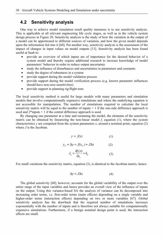
30 Aircraft Vehicle Systems Modeling and Simulation under uncertainty
4.2 Sensitivity analysis
One way to achieve model simulation result quality measures is to use sensitivity analysis. This is applicable at all relevant engineering life cycle stages, as well as in the vehicle system design process in Figure 20. Sensitivity analysis is the study of how the variation in the output of a model can be apportioned to different sources of variation, and how the given model depends upon the information fed into it [60]. Put another way, sensitivity analysis is the assessment of the impact of changes in input values on model outputs [13]. Sensitivity analysis has been found useful at Saab to:
• provide an overview of which inputs are of importance for the desired behavior of a system model and thereby require additional research to increase knowledge of model parameters’ behavior in order to reduce output uncertainty
• study the influence of disturbances and uncertainties in parameters and constants • study the degree of robustness in a system • provide support during the model validation process • provide support during the model verification process (e.g. known parameter influences
should have non-zero sensitivities) • provide support in planning rig/flight tests
The local sensitivity method is useful for large models with many parameters and simulation models that involve computationally expensive simulations and where the underlying equation is not accessible for manipulation. The number of simulations required to calculate the local sensitivity matrix will be equal to the number of inputs + 1 if the one-side difference approach is used and 2*inputs + 1 if the central difference approach is used.
By changing one parameter at a time and rerunning the model, the elements of the sensitivity matrix can be obtained by linearizing the non-linear model f, equation (1), where the system characteristics y are computed from the system parameters x, around a nominal point, equation (2) where J is the Jacobian.
f(x)y = (1)
xJ)f(x y y 00 Δ+=Δ+ (2)
ijj
iij k
x
xfJ =
∂∂= )(
(3)
For small variations the sensitivity matrix, equation (3), is identical to the Jacobian matrix, hence:
xJ y Δ=Δ (4)
The global sensitivity [60], however, accounts for the global variability of the output over the entire range of the input variables and hence provides an overall view of the influence of inputs on the output. Using this variance-based SA the analysis of variance can be decomposed into increasing order terms, i.e. first-order terms (main effects) depending on a single variable and higher-order terms (interaction effects) depending on two or more variables [67]. Global sensitivity analysis has the drawback that the required number of simulations increases exponentially with the number of inputs and is therefore not always suitable for computationally expensive simulations. Furthermore, if a benign nominal design point is used, the interaction effects are small.
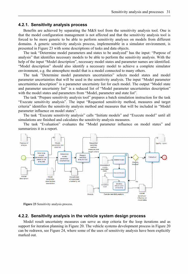
Sensitivity analysis and processes 31
4.2.1. Sensitivity analysis process Benefits are achieved by separating the M&S tool from the sensitivity analysis tool. One is
that the model configuration management is not affected and that the sensitivity analysis tool is forced to be more generic to be able to perform sensitivity analyses on models from different domains. A generic sensitivity analysis process, implementable in a simulator environment, is presented in Figure 23 with some descriptions of tasks and data objects.
The task “Determine model parameters and states to be analyzed” has the input: “Purpose of analysis” that identifies necessary models to be able to perform the sensitivity analysis. With the help of the input “Model description”, necessary model states and parameter names are identified. “Model description” should also identify a necessary model to achieve a complete simulator environment, e.g. the atmosphere model that is a model connected to many others.
The task ”Determine model parameters uncertainties” selects model states and model parameter uncertainties that will be used in the sensitivity analysis. The input “Model parameter uncertainties description” is a parameter uncertainty list for each model. The output “Model state and parameter uncertainty list” is a reduced list of “Model parameter uncertainties description” with the model states and parameters from “Model, parameter and state list”.
The task “Prepare sensitivity analysis tool” prepares a batch simulation instruction for the task “Execute sensitivity analysis”. The input “Requested sensitivity method, measures and target criteria” identifies the sensitivity analysis method and measures that will be included in “Model parameter influence on model states”.
The task “Execute sensitivity analysis” calls “Initiate models” and “Execute model” until all simulations are finished and calculates the sensitivity analysis measures.
The task “Evaluation” evaluates the “Model parameter influence on model states” and summarizes it in a report.
Figure 23 Sensitivity analysis process.
4.2.2. Sensitivity analysis in the vehicle system design process Model result uncertainty measures can serve as stop criteria for the loop iterations and as
support for iteration planning in Figure 20. The vehicle systems development process in Figure 20 can be redrawn, see Figure 24, where some of the uses of sensitivity analysis have been explicitly marked out.
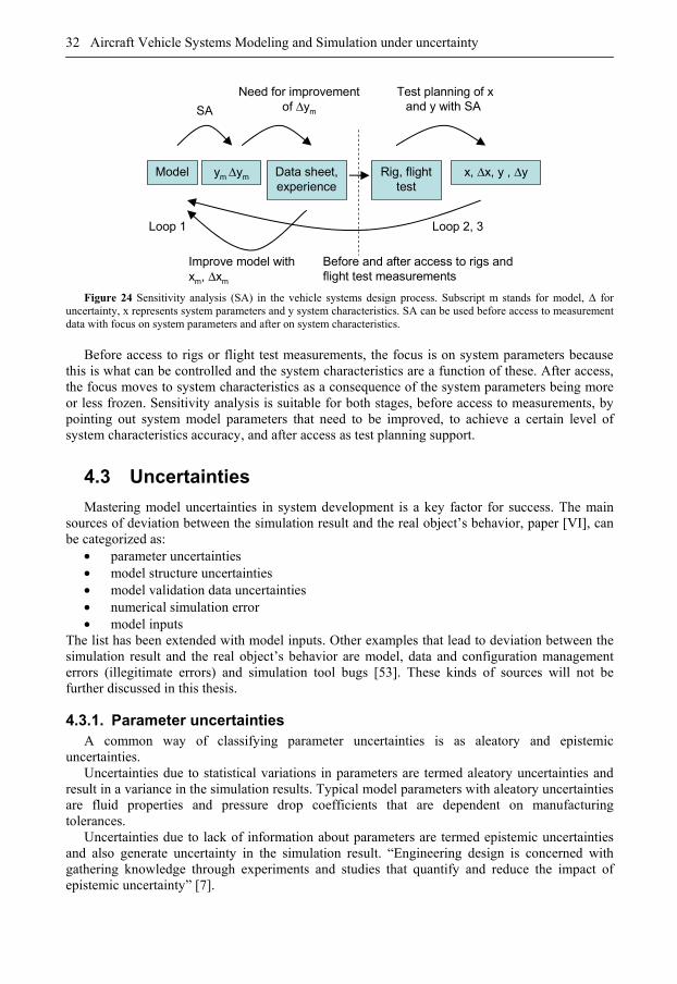
32 Aircraft Vehicle Systems Modeling and Simulation under uncertainty
Model ym Δym
SA
Data sheet, experience
Need for improvement of Δym
Test planning of x and y with SA
x, Δx, y , ΔyRig, flight test
Improve model with xm, Δxm
Before and after access to rigs and flight test measurements
Loop 2, 3Loop 1
Figure 24 Sensitivity analysis (SA) in the vehicle systems design process. Subscript m stands for model, Δ for
uncertainty, x represents system parameters and y system characteristics. SA can be used before access to measurement data with focus on system parameters and after on system characteristics.
Before access to rigs or flight test measurements, the focus is on system parameters because
this is what can be controlled and the system characteristics are a function of these. After access, the focus moves to system characteristics as a consequence of the system parameters being more or less frozen. Sensitivity analysis is suitable for both stages, before access to measurements, by pointing out system model parameters that need to be improved, to achieve a certain level of system characteristics accuracy, and after access as test planning support.
4.3 Uncertainties
Mastering model uncertainties in system development is a key factor for success. The main sources of deviation between the simulation result and the real object’s behavior, paper [VI], can be categorized as:
• parameter uncertainties • model structure uncertainties • model validation data uncertainties • numerical simulation error • model inputs
The list has been extended with model inputs. Other examples that lead to deviation between the simulation result and the real object’s behavior are model, data and configuration management errors (illegitimate errors) and simulation tool bugs [53]. These kinds of sources will not be further discussed in this thesis.
4.3.1. Parameter uncertainties A common way of classifying parameter uncertainties is as aleatory and epistemic
uncertainties. Uncertainties due to statistical variations in parameters are termed aleatory uncertainties and
result in a variance in the simulation results. Typical model parameters with aleatory uncertainties are fluid properties and pressure drop coefficients that are dependent on manufacturing tolerances.
Uncertainties due to lack of information about parameters are termed epistemic uncertainties and also generate uncertainty in the simulation result. “Engineering design is concerned with gathering knowledge through experiments and studies that quantify and reduce the impact of epistemic uncertainty” [7].
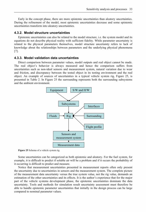
Sensitivity analysis and processes 33
Early in the concept phase, there are more epistemic uncertainties than aleatory uncertainties. During the refinement of the model, most epistemic uncertainties decrease and some epistemic uncertainties transform into aleatory uncertainties.
4.3.2. Model structure uncertainties Epistemic uncertainties can also be related to the model structure, i.e. the system model and its
equations do not describe physical reality with sufficient fidelity. While parameter uncertainty is related to the physical parameters themselves, model structure uncertainty refers to lack of knowledge about the relationships between parameters and the underlying physical phenomena [7].
4.3.3. Model validation data uncertainties Direct comparison between parameter values, model outputs and real object cannot be made.
The real object’s behavior is always measured and hence the comparison suffers from uncertainties such as non-ideal sensors and measurement system, natural variation due to wear and friction, and discrepancy between the tested object in its testing environment and the real object. An example of sources of uncertainties in a typical vehicle system rig, Figure 25, is presented in Table 2. In Figure 25 the surrounding represents both the surrounding subsystems and the ambient environment.
Flight profile
Subsystems
Rig
Equipment
Measurement data
Interfaces
Surrounding
S/W and H/W
Fluids
Sensors and measurement system
Figure 25 Schema of a vehicle system rig. Some uncertainties can be categorized as both epistemic and aleatory. For the fuel system, for
example, it is difficult to predict if soluble air will be a problem and if it occurs the probability of it occurring is difficult to predict and measure.
Notice that measurement uncertainties presented in measurement reports often only present the uncertainty due to uncertainties in sensors and the measurement system. The complete picture of the measurement data uncertainty versus the true system value, not the rig value, demands an estimation of the other uncertainties and its effects. It is the author’s experience that for the major part of the vehicle systems development phase, the epistemic uncertainties dominate the data uncertainty. Tools and methods for simulation result uncertainty assessment must therefore be able to handle epistemic parameter uncertainties that initially in the design process can be large compared to nominal parameter values.
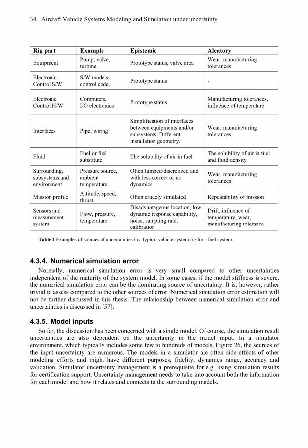
34 Aircraft Vehicle Systems Modeling and Simulation under uncertainty
Table 2 Examples of sources of uncertainties in a typical vehicle system rig for a fuel system.
4.3.4. Numerical simulation error Normally, numerical simulation error is very small compared to other uncertainties
independent of the maturity of the system model. In some cases, if the model stiffness is severe, the numerical simulation error can be the dominating source of uncertainty. It is, however, rather trivial to assess compared to the other sources of error. Numerical simulation error estimation will not be further discussed in this thesis. The relationship between numerical simulation error and uncertainties is discussed in [57].
4.3.5. Model inputs So far, the discussion has been concerned with a single model. Of course, the simulation result
uncertainties are also dependent on the uncertainty in the model input. In a simulator environment, which typically includes some few to hundreds of models, Figure 26, the sources of the input uncertainty are numerous. The models in a simulator are often side-effects of other modeling efforts and might have different purposes, fidelity, dynamics range, accuracy and validation. Simulator uncertainty management is a prerequisite for e.g. using simulation results for certification support. Uncertainty management needs to take into account both the information for each model and how it relates and connects to the surrounding models.
Rig part Example Epistemic Aleatory
Equipment Pump, valve, turbine
Prototype status, valve area Wear, manufacturing tolerances
Electronic Control S/W
S/W models, control code,
Prototype status -
Electronic Control H/W
Computers, I/O electronics
Prototype status Manufacturing tolerances, influence of temperature
Interfaces Pipe, wiring
Simplification of interfaces between equipments and/or subsystems. Different installation geometry.
Wear, manufacturing tolerances
Fluid Fuel or fuel substitute
The solubility of air in fuel The solubility of air in fuel and fluid density
Surrounding, subsystems and environment
Pressure source, ambient temperature
Often lumped/discretized and with less correct or no dynamics
Wear, manufacturing tolerances
Mission profile Altitude, speed, thrust
Often crudely simulated Repeatability of mission
Sensors and measurement system
Flow, pressure, temperature
Disadvantageous location, low dynamic response capability, noise, sampling rate, calibration
Drift, influence of temperature, wear, manufacturing tolerance
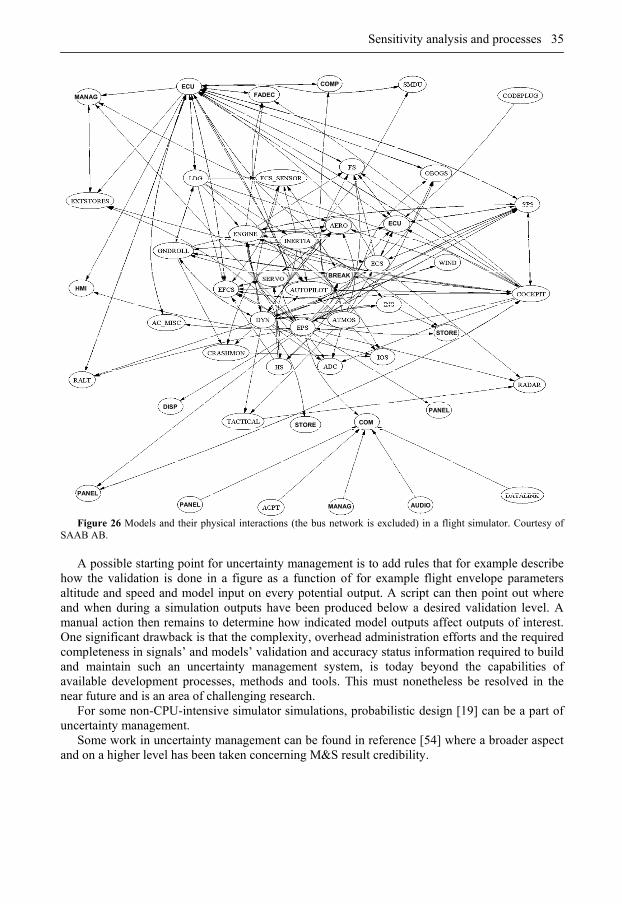
Sensitivity analysis and processes 35
ECU
MANAG FADEC
PANEL
ECU
COMP
HMI
STORE
BREAK
COM
AUDIOPANEL MANAG
PANELDISP
STORE
Figure 26 Models and their physical interactions (the bus network is excluded) in a flight simulator. Courtesy of
SAAB AB. A possible starting point for uncertainty management is to add rules that for example describe
how the validation is done in a figure as a function of for example flight envelope parameters altitude and speed and model input on every potential output. A script can then point out where and when during a simulation outputs have been produced below a desired validation level. A manual action then remains to determine how indicated model outputs affect outputs of interest. One significant drawback is that the complexity, overhead administration efforts and the required completeness in signals’ and models’ validation and accuracy status information required to build and maintain such an uncertainty management system, is today beyond the capabilities of available development processes, methods and tools. This must nonetheless be resolved in the near future and is an area of challenging research.
For some non-CPU-intensive simulator simulations, probabilistic design [19] can be a part of uncertainty management.
Some work in uncertainty management can be found in reference [54] where a broader aspect and on a higher level has been taken concerning M&S result credibility.
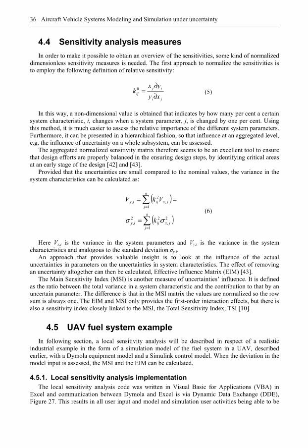
36 Aircraft Vehicle Systems Modeling and Simulation under uncertainty
4.4 Sensitivity analysis measures
In order to make it possible to obtain an overview of the sensitivities, some kind of normalized dimensionless sensitivity measures is needed. The first approach to normalize the sensitivities is to employ the following definition of relative sensitivity:
ji
ijij xy
yxk
∂∂
=0 (5)
In this way, a non-dimensional value is obtained that indicates by how many per cent a certain
system characteristic, i, changes when a system parameter, j, is changed by one per cent. Using this method, it is much easier to assess the relative importance of the different system parameters. Furthermore, it can be presented in a hierarchical fashion, so that influence at an aggregated level, e.g. the influence of uncertainty on a whole subsystem, can be assessed.
The aggregated normalized sensitivity matrix therefore seems to be an excellent tool to ensure that design efforts are properly balanced in the ensuring design steps, by identifying critical areas at an early stage of the design [42] and [43].
Provided that the uncertainties are small compared to the nominal values, the variance in the system characteristics can be calculated as:
( )
( )
=
=
=
==
n
jjxijiy
n
jjxijiy
k
VkV
1
2,
22,
1,
2,
σσ (6)
Here Vx,j is the variance in the system parameters and Vy,i is the variance in the system
characteristics and analogous to the standard deviation σy,i. An approach that provides valuable insight is to look at the influence of the actual
uncertainties in parameters on the uncertainties in system characteristics. The effect of removing an uncertainty altogether can then be calculated, Effective Influence Matrix (EIM) [43].
The Main Sensitivity Index (MSI) is another measure of uncertainties’ influence. It is defined as the ratio between the total variance in a system characteristic and the contribution to that by an uncertain parameter. The difference is that in the MSI matrix the values are normalized so the row sum is always one. The EIM and MSI only provides the first-order interaction effects, but there is also a sensitivity index closely linked to the MSI, the Total Sensitivity Index, TSI [10].
4.5 UAV fuel system example
In following section, a local sensitivity analysis will be described in respect of a realistic industrial example in the form of a simulation model of the fuel system in a UAV, described earlier, with a Dymola equipment model and a Simulink control model. When the deviation in the model input is assessed, the MSI and the EIM can be calculated.
4.5.1. Local sensitivity analysis implementation The local sensitivity analysis code was written in Visual Basic for Applications (VBA) in
Excel and communication between Dymola and Excel is via Dynamic Data Exchange (DDE), Figure 27. This results in all user input and model and simulation user activities being able to be
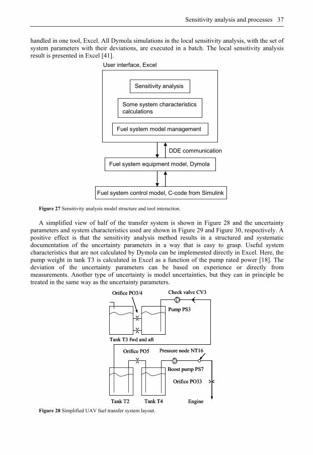
Sensitivity analysis and processes 37
handled in one tool, Excel. All Dymola simulations in the local sensitivity analysis, with the set of system parameters with their deviations, are executed in a batch. The local sensitivity analysis result is presented in Excel [41].
User interface, Excel
Sensitivity analysis
Some system characteristics calculations
Fuel system model management
Fuel system equipment model, Dymola
Fuel system control model, C-code from Simulink
DDE communication
Figure 27 Sensitivity analysis model structure and tool interaction. A simplified view of half of the transfer system is shown in Figure 28 and the uncertainty
parameters and system characteristics used are shown in Figure 29 and Figure 30, respectively. A positive effect is that the sensitivity analysis method results in a structured and systematic documentation of the uncertainty parameters in a way that is easy to grasp. Useful system characteristics that are not calculated by Dymola can be implemented directly in Excel. Here, the pump weight in tank T3 is calculated in Excel as a function of the pump rated power [18]. The deviation of the uncertainty parameters can be based on experience or directly from measurements. Another type of uncertainty is model uncertainties, but they can in principle be treated in the same way as the uncertainty parameters.
Orifice PO3/4
Pump PS3
Check valve CV3
Orifice PO5
Boost pump PS7
Engine
Pressure node NT16
Tank T4
Tank T3 fwd and aft
Tank T2
Orifice PO33
Orifice PO3/4
Pump PS3
Check valve CV3
Orifice PO5
Boost pump PS7
Engine
Pressure node NT16
Tank T4
Tank T3 fwd and aft
Tank T2
Orifice PO33
Figure 28 Simplified UAV fuel transfer system layout.
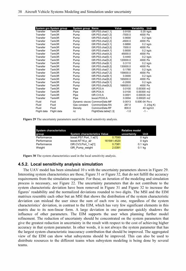
38 Aircraft Vehicle Systems Modeling and Simulation under uncertainty
System gro System group System group Name Value Variability UnitTransfer Tank3R Pump t3R.PS3.char[1,1] 0.9100 0.20 kg/sTransfer Tank3R Pump t3R.PS3.char[1,2] -7000.0 4000 PaTransfer Tank3R Pump t3R.PS3.char[2,1] 0.9000 0.2 kg/sTransfer Tank3R Pump t3R.PS3.char[2,2] -4500.0 4000 PaTransfer Tank3R Pump t3R.PS3.char[3,1] 0.8890 0.2 kg/sTransfer Tank3R Pump t3R.PS3.char[3,2] 7000.0 4000 PaTransfer Tank3R Pump t3R.PS3.char[4,1] 0.8000 0.2 kg/sTransfer Tank3R Pump t3R.PS3.char[4,2] 45000.0 4000 PaTransfer Tank3R Pump t3R.PS3.char[5,1] 0.4440 0.2 kg/sTransfer Tank3R Pump t3R.PS3.char[5,2] 120000.0 4000 PaTransfer Tank3R Pump t3R.PS3.char[6,1] 0.3110 0.2 kg/sTransfer Tank3R Pump t3R.PS3.char[6,2] 130000.0 4000 PaTransfer Tank3R Pump t3R.PS3.char[7,1] 0.1780 0.2 kg/sTransfer Tank3R Pump t3R.PS3.char[7,2] 159000.0 4000 PaTransfer Tank3R Pump t3R.PS3.char[8,1] 0.0000 0.2 kg/sTransfer Tank3R Pump t3R.PS3.char[8,2] 165000.0 4000 PaTransfer Tank3R Pump t3R.PS3.char[9,1] -0.2000 0.2 kg/sTransfer Tank3R Pump t3R.PS3.char[9,2] 168000.0 4000 PaTransfer Tank3R Pipe t3R.PO3.A 0.0100 0.00300 m2Transfer Tank3R Pipe t3R.PO4.A 0.0100 0.00300 m2Transfer Tank3R Pipe t3R.CV3.A 0.0001 0.00035 m2Transfer Tank4R Pipe boost.PO33.A 0.0004 0.00020 m2Fluid Fluid Dynamic viscosiCommonData.MF 0.0013 5.00E-04 Pa sFluid Fluid Gas constant CommonData.RA 287.0 3 J/(kg K)Fluid Fluid Density CommonData.RF 800.0 40 kg/m3Flight data Flight data nz FlightData.table[1,3] -1.0 -1 -
Figure 29 The uncertainty parameters used in the local sensitivity analysis.
System characteristics group System characteristics Value
Relative model uncertainty Unit
Performance boost.PS7.Port_1.w[1] 0.7590 0 kg/sPerformance boost.NT16.p_air 161841.4520 0 kg/sPerformance t3R.CV3.Port_1.w[1] 0.7381 0.1 kg/sWeight t3R_Pump_weight 2.0391 0.1 kg
Figure 30 The system characteristics used in the local sensitivity analysis.
4.5.2. Local sensitivity analysis simulation The UAV model has been simulated 10 s with the uncertainty parameters shown in Figure 29.
Interesting system characteristics are those, Figure 31 or Figure 32, that do not fulfill the accuracy requirements from the simulation requester. For these, an iteration of the modeling and simulation process is necessary, see Figure 22. The uncertainty parameters that do not contribute to the system characteristic deviation have been removed in Figure 31 and Figure 32 to increase the figures’ readability and the normalized deviations rounded to two digits. The MSI and the EIM matrixes resemble each other but an MSI that shows the distribution of the system characteristic deviation can mislead the user since the sum of each row is one, regardless of the system characteristics’ deviation, in contrast to the EIM, which has very few significant elements in this matrix due to its non-linear form. A large deviation in one parameter quickly shadows the influence of other parameters. The EIM supports the user when planning further model refinement. The reduction of uncertainty should be concentrated on the system parameters that give the greatest reduction in uncertainty in the result with respect to the cost of achieving higher accuracy in that system parameter. In other words, it is not always the system parameter that has the largest system characteristic inaccuracy contribution that should be improved. The aggregated view of the EIM can show what subsystems should be improved. This can also be used to distribute resources to the different teams when subsystem modeling is being done by several teams.
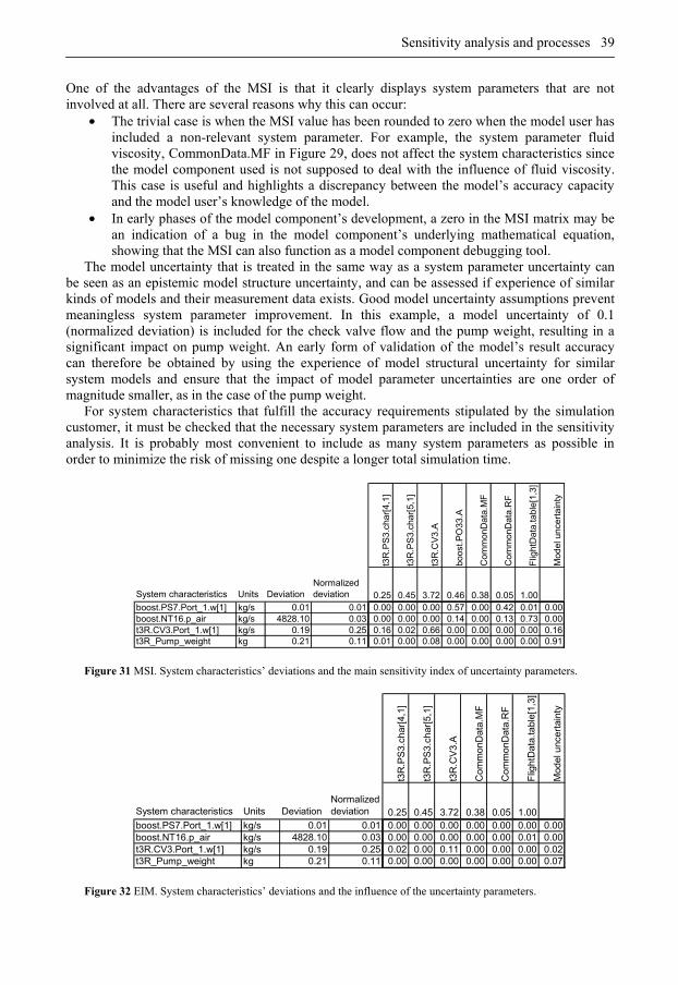
Sensitivity analysis and processes 39
One of the advantages of the MSI is that it clearly displays system parameters that are not involved at all. There are several reasons why this can occur:
• The trivial case is when the MSI value has been rounded to zero when the model user has included a non-relevant system parameter. For example, the system parameter fluid viscosity, CommonData.MF in Figure 29, does not affect the system characteristics since the model component used is not supposed to deal with the influence of fluid viscosity. This case is useful and highlights a discrepancy between the model’s accuracy capacity and the model user’s knowledge of the model.
• In early phases of the model component’s development, a zero in the MSI matrix may be an indication of a bug in the model component’s underlying mathematical equation, showing that the MSI can also function as a model component debugging tool.
The model uncertainty that is treated in the same way as a system parameter uncertainty can be seen as an epistemic model structure uncertainty, and can be assessed if experience of similar kinds of models and their measurement data exists. Good model uncertainty assumptions prevent meaningless system parameter improvement. In this example, a model uncertainty of 0.1 (normalized deviation) is included for the check valve flow and the pump weight, resulting in a significant impact on pump weight. An early form of validation of the model’s result accuracy can therefore be obtained by using the experience of model structural uncertainty for similar system models and ensure that the impact of model parameter uncertainties are one order of magnitude smaller, as in the case of the pump weight.
For system characteristics that fulfill the accuracy requirements stipulated by the simulation customer, it must be checked that the necessary system parameters are included in the sensitivity analysis. It is probably most convenient to include as many system parameters as possible in order to minimize the risk of missing one despite a longer total simulation time.
t3R
.PS
3.ch
ar[4
,1]
t3R
.PS
3.ch
ar[5
,1]
t3R
.CV
3.A
boos
t.PO
33.A
Com
mon
Dat
a.M
F
Com
mon
Dat
a.R
F
Flig
htD
ata.
tabl
e[1,
3]
Mod
el u
ncer
tain
ty
System characteristics Units DeviationNormalized deviation 0.25 0.45 3.72 0.46 0.38 0.05 1.00
boost.PS7.Port_1.w[1] kg/s 0.01 0.01 0.00 0.00 0.00 0.57 0.00 0.42 0.01 0.00boost.NT16.p_air kg/s 4828.10 0.03 0.00 0.00 0.00 0.14 0.00 0.13 0.73 0.00t3R.CV3.Port_1.w[1] kg/s 0.19 0.25 0.16 0.02 0.66 0.00 0.00 0.00 0.00 0.16t3R_Pump_weight kg 0.21 0.11 0.01 0.00 0.08 0.00 0.00 0.00 0.00 0.91
Figure 31 MSI. System characteristics’ deviations and the main sensitivity index of uncertainty parameters.
t3R
.PS
3.ch
ar[4
,1]
t3R
.PS
3.ch
ar[5
,1]
t3R
.CV
3.A
Com
mon
Dat
a.M
F
Com
mon
Dat
a.R
F
Flig
htD
ata.
tabl
e[1
,3]
Mod
el u
ncer
tain
ty
System characteristics Units DeviationNormalized deviation 0.25 0.45 3.72 0.38 0.05 1.00
boost.PS7.Port_1.w[1] kg/s 0.01 0.01 0.00 0.00 0.00 0.00 0.00 0.00 0.00boost.NT16.p_air kg/s 4828.10 0.03 0.00 0.00 0.00 0.00 0.00 0.01 0.00t3R.CV3.Port_1.w[1] kg/s 0.19 0.25 0.02 0.00 0.11 0.00 0.00 0.00 0.02t3R_Pump_weight kg 0.21 0.11 0.00 0.00 0.00 0.00 0.00 0.00 0.07
Figure 32 EIM. System characteristics’ deviations and the influence of the uncertainty parameters.
40 Aircraft Vehicle Systems Modeling and Simulation under uncertainty
4.6 Summary
The need for uncertainty management and more complete validation methods that complement traditional validation, knowledge of a model’s maturity and simulation result accuracy, has emerged due to the intensity of M&S that MBSE has in early vehicle systems development phases. Resolving this need is important to succeed in system development where early design decisions have to be made supported by simulation only. The ability to handle uncertain information and lack of information is the key to success in early design.
Further, the local sensitivity method has been shown to be useful for large models with many parameters and simulation models that involve computationally expensive simulations. One side-benefit of using sensitivity analysis is that the unexpected absence of sensitivity in parameters might indicate a modeling error and it is therefore also a valuable debugging tool for models.
Discussion and Conclusions 41
5
Discussion and
Conclusions
HE VEHICLE SYSTEM PROCESS presented in paper [II] covers almost the whole general design process, excluding the specification and production phases. The remaining presented
papers [I], [III] and [IV] can be fitted into this process, Figure 33. The relationship between the methods, techniques and processes described in this thesis, as well as where in the vehicle system process they are applicable, can then be displayed. Paper [I] describes hosted simulation, that enables system simulation with models from different domains to be used in the first loop. Paper [II] describes the context where proposed methods will be used. Finally, papers [III] and [IV] describe sources of uncertainty and sensitivity analysis that are useful in all three loops with a focus on physical system models but with less attention paid to how the behavior of s/w models affects the suitability of sensitivity analysis in the design process.
T
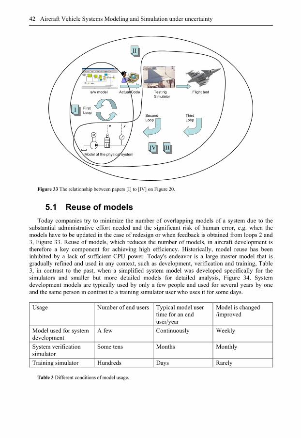
42 Aircraft Vehicle Systems Modeling and Simulation under uncertainty
Flight test
First Loop
SecondLoop
ThirdLoop
Model of the physical system
Actual Codes/w model
M
u y
M
u y
Test rigSimulator
IIIIIIIVIV
II
II
Figure 33 The relationship between papers [I] to [IV] on Figure 20.
5.1 Reuse of models
Today companies try to minimize the number of overlapping models of a system due to the substantial administrative effort needed and the significant risk of human error, e.g. when the models have to be updated in the case of redesign or when feedback is obtained from loops 2 and 3, Figure 33. Reuse of models, which reduces the number of models, in aircraft development is therefore a key component for achieving high efficiency. Historically, model reuse has been inhibited by a lack of sufficient CPU power. Today's endeavor is a large master model that is gradually refined and used in any context, such as development, verification and training, Table 3, in contrast to the past, when a simplified system model was developed specifically for the simulators and smaller but more detailed models for detailed analysis, Figure 34. System development models are typically used by only a few people and used for several years by one and the same person in contrast to a training simulator user who uses it for some days. Usage Number of end users Typical model user
time for an end user/year
Model is changed /improved
Model used for system development
A few Continuously Weekly
System verification simulator
Some tens Months Monthly
Training simulator Hundreds Days Rarely
Table 3 Different conditions of model usage.
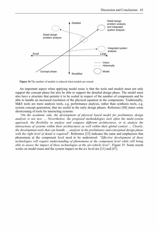
Discussion and Conclusions 43
Small
Detailed
Simplified
Large
Concept phase
Detail design problem analysis
Integrated system analysis
VisionHistorically
Model
Detail design problem analysis and integrated system analysis
Figure 34 The number of models is reduced when models are reused. An important aspect when applying model reuse is that the tools and models must not only
support the concept phase but also be able to support the detailed design phase. The model must also have a structure that permits it to be scaled in respect of the number of components and be able to handle an increased resolution of the physical equation in the components. Traditionally, M&S tools are more analysis tools, e.g. performance analysis, rather than synthesis tools, e.g. system concept generation, that are useful in the early design phases. Reference [48] states some shortcoming of tools for interacting systems:
“On the academic side, the development of physical based model for preliminary design analysis is not new … Nevertheless, the proposed methodologies lack often the multi-system approach, the flexibility to analyze and compare different architectures, or to analyze the interactions of systems within their architectures as well within their global context … Clearly, the development tools that can handle … analysis in the preliminary and conceptual design phase with the right level of detail is required”. Reference [23] indicates the same and emphasizes that phenomena at the component level need to be understood: “Effective development of these technologies will require understanding of phenomena at the component level while still being able to assess the impact of these technologies at the air-vehicle level”, Figure 35. Some recent works on model reuse and the system impact on the a/c level are [21] and [47].
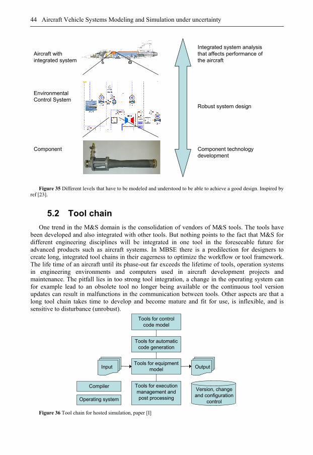
44 Aircraft Vehicle Systems Modeling and Simulation under uncertainty
EnvironmentalControl System
Component
Aircraft with integrated system
Integrated system analysis that affects performance of the aircraft
Robust system design
Component technology development
Figure 35 Different levels that have to be modeled and understood to be able to achieve a good design. Inspired by ref [23].
5.2 Tool chain
One trend in the M&S domain is the consolidation of vendors of M&S tools. The tools have been developed and also integrated with other tools. But nothing points to the fact that M&S for different engineering disciplines will be integrated in one tool in the foreseeable future for advanced products such as aircraft systems. In MBSE there is a predilection for designers to create long, integrated tool chains in their eagerness to optimize the workflow or tool framework. The life time of an aircraft until its phase-out far exceeds the lifetime of tools, operation systems in engineering environments and computers used in aircraft development projects and maintenance. The pitfall lies in too strong tool integration, a change in the operating system can for example lead to an obsolete tool no longer being available or the continuous tool version updates can result in malfunctions in the communication between tools. Other aspects are that a long tool chain takes time to develop and become mature and fit for use, is inflexible, and is sensitive to disturbance (unrobust).
Tools for control code model
Tools for equipment model
Compiler
Operating system
Input Output
Version, changeand configuration
control
Tools for execution management and post processing
Tools for automatic code generation
Figure 36 Tool chain for hosted simulation, paper [I]
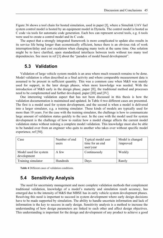
Discussion and Conclusions 45
Figure 36 shows a tool chain for hosted simulation, used in paper [I], where a Simulink UAV fuel system control model is hosted by an equipment model in Dymola. The control model is hosted as C code via tools for automatic code generation. Each box can represent several tools, e.g. 6 tools were used to create a control model and its C code.
The aspect that a strongly integrated framework is more complicated to update also results in its service life being longer than economically efficient, hence there is an obvious risk of work interruption/delay and cost escalation when changing many tools at the same time. One solution might be to have clarified, open standardized interfaces between tools without too many tool dependencies. See more in ref [3] about the “paradox of model based development”.
5.3 Validation
Validation of large vehicle system models is an area where much research remains to be done. Model validation is often described as a final activity and where comparable measurement data is assumed to be present in sufficient quantity. This was a common case when M&S was mainly used for support, in the later design phases, when more knowledge was needed. With the introduction of M&S early in the design phase, paper [II], the traditional method and processes need to be complemented and further developed, paper [III] and [IV].
One interesting validation aspect that has not been discussed in this thesis is how the validation documentation is maintained and updated. In Table 4 two different cases are presented. The first is a model used for system development, and the second is when a model is delivered into a larger simulator, e.g. a training simulator. These kinds of models are typically used for more than 10 years. For the case with the training simulator, the challenge is how to communicate large amount of validation status quickly to the user. In the case with the model used for system development is the challenge of how to realize how a model change affects the current model validation status without redoing a complete model validation. This knowledge must also be able to be handed over from an engineer who quits to another who takes over without specific model experience, ref [50].
Case Number of end users
Typical model user time for an end user/year
Model is changed /improved
Model used for system development
A few Continuously Weekly
Training simulator Hundreds Days Rarely Table 4 Different cases of validation conditions.
5.4 Sensitivity Analysis
The need for uncertainty management and more complete validation methods that complement traditional validation, knowledge of a model’s maturity and simulation result accuracy, has emerged due to the intensity of M&S that MBSE has in early vehicle system development phases. Resolving this need is important to succeed in system development where early design decisions have to be made supported by simulation. The ability to handle uncertain information and lack of information is the key to success in early design. Sensitivity analysis is a method to increase the understanding of how design parameters are linked to each other and affect design objectives. This understanding is important for the design and development of any product to achieve a good
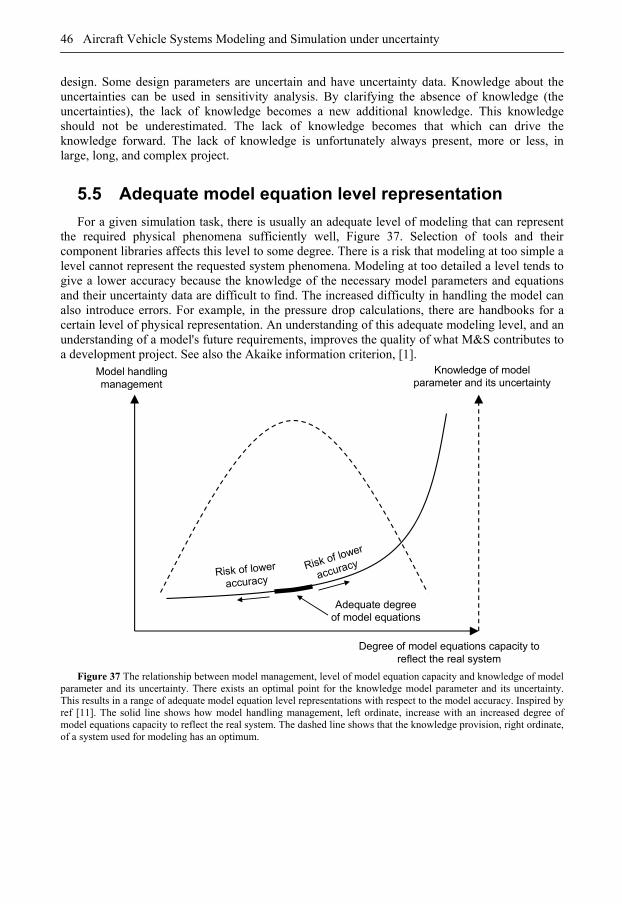
46 Aircraft Vehicle Systems Modeling and Simulation under uncertainty
design. Some design parameters are uncertain and have uncertainty data. Knowledge about the uncertainties can be used in sensitivity analysis. By clarifying the absence of knowledge (the uncertainties), the lack of knowledge becomes a new additional knowledge. This knowledge should not be underestimated. The lack of knowledge becomes that which can drive the knowledge forward. The lack of knowledge is unfortunately always present, more or less, in large, long, and complex project.
5.5 Adequate model equation level representation
For a given simulation task, there is usually an adequate level of modeling that can represent the required physical phenomena sufficiently well, Figure 37. Selection of tools and their component libraries affects this level to some degree. There is a risk that modeling at too simple a level cannot represent the requested system phenomena. Modeling at too detailed a level tends to give a lower accuracy because the knowledge of the necessary model parameters and equations and their uncertainty data are difficult to find. The increased difficulty in handling the model can also introduce errors. For example, in the pressure drop calculations, there are handbooks for a certain level of physical representation. An understanding of this adequate modeling level, and an understanding of a model's future requirements, improves the quality of what M&S contributes to a development project. See also the Akaike information criterion, [1].
Model handling management
Degree of model equations capacity to reflect the real system
Knowledge of model parameter and its uncertainty
Adequate degree of model equations
Risk of lower
accuracyRisk of lower
accuracy
Figure 37 The relationship between model management, level of model equation capacity and knowledge of model
parameter and its uncertainty. There exists an optimal point for the knowledge model parameter and its uncertainty. This results in a range of adequate model equation level representations with respect to the model accuracy. Inspired by ref [11]. The solid line shows how model handling management, left ordinate, increase with an increased degree of model equations capacity to reflect the real system. The dashed line shows that the knowledge provision, right ordinate, of a system used for modeling has an optimum.
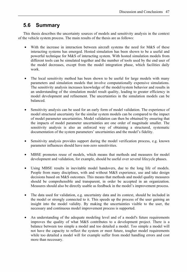
Discussion and Conclusions 47
5.6 Summary
This thesis describes the uncertainty sources of models and sensitivity analysis in the context of the vehicle system process. The main results of the thesis are as follows:
• With the increase in interaction between aircraft systems the need for M&S of these
interacting systems has emerged. Hosted simulation has been shown to be a useful and powerful technique for M&S of interacting system. With hosted simulation models from different tools can be simulated together and the number of tools used by the end user of the model decreases, except from the model integration phase, which facilities daily work.
• The local sensitivity method has been shown to be useful for large models with many
parameters and simulation models that involve computationally expensive simulations. The sensitivity analysis increases knowledge of the model/system behavior and results in an understanding of the simulation model result quality, leading to greater efficiency in model development and refinement. The uncertainties in the simulation models can be balanced.
• Sensitivity analysis can be used for an early form of model validation. The experience of
model structural uncertainty for the similar system models can be compared to the impact of model parameter uncertainties. Model validation can then be obtained by ensuring that the impacts of model parameter uncertainties are one order of magnitude smaller. The sensitivity analysis is also an enforced way of obtaining a structured, systematic documentation of the system parameters’ uncertainties and the model’s fidelity.
• Sensitivity analysis provides support during the model verification process, e.g. known
parameter influences should have non-zero sensitivities.
• MBSE promotes reuse of models, which means that methods and measures for model development and validation, for example, should be useful over several lifecycle phases.
• Using MBSE results in inevitable model handovers, due to the long life of models.
People from many disciplines, with and without M&S experience, use and take design decisions based on M&S outcomes. This means that methods and model quality measures should be comprehensible and transparent, in order be accepted in an organization. Measures should also be directly usable as feedback in the model’s improvement process.
• The data used for validation, e.g. uncertainty data and its context, should be included in
the model or strongly connected to it. This speeds up the process of the user gaining an insight into the model validity. By making the uncertainties visible to the user, the necessary and continuous model improvement process is supported.
• An understanding of the adequate modeling level and of a model's future requirements
improves the quality of what M&S contributes to a development project. There is a balance between too simple a model and too detailed a model. Too simple a model will not have the capacity to reflect the system or meet future, tougher model requirements while too detailed a model will for example suffer from model handling errors and cost more than necessary.
48 Aircraft Vehicle Systems Modeling and Simulation under uncertainty
5.7 Future work
Sensitivity analysis of a model by a user who lacks experience of or insight into the model can be problematic. An analysis which demonstrates the absence of a model parameter's impact on the simulation results can be correct, but also demonstrates a lack of model representation of the modeled system. To recognize when this occurs is difficult for the user.
So far, the discussion has been concerned with a single model. Of course, the simulation result uncertainties are also dependent on the uncertainty in the model input. In a simulator environment, which typically includes some few to hundreds of models, Figure 26, the sources of the input uncertainty are numerous. The models in a simulator are often side-effects of other modeling efforts and might have different purposes, fidelity, dynamics range, accuracy, and validation. Simulator uncertainty management is a prerequisite for using simulation results for certification support for example. Uncertainty management needs to take into account both the information for each model and how it relates and connects to the surrounding models. Substantial challenges remain, both for the user and the method and process developer, before uncertainties can be used in system simulators. Some challenges are the difficulty to achieve the desired completeness in models’ validation status and signals uncertainties description and suitable validation and accuracy measures.
One of the main problems to solve is that a model can be validated outside a simulator but implemented in a simulator, where it can be fed by input from another model with unknown accuracy. It is tempting to use the phrase “garbage in, garbage out”. A first step in taking control of the model’s input accuracy in a simulator is to classify the models of the simulator output’s quality, paper [IV], into a meta-model, Figure 38 ref [40]. If these meta-models are then executed in parallel with the usual simulation quality, information can be obtained about a model's output, for example if a model delivered output of lower quality at a speed close to Mach 1 during a flight case. If this is then combined with a meta-model of the simulator model couplings, affected models can also to some extent be pointed out.
Mach 1
Alt
Mach
Increased model output quality
Figure 38 A model that classifies the model’s output quality. For example, in the simulator the aero data model output for transonic passages is difficult to calculate and the simulator is therefore a bad environment for testing transonic handling quality for models that use data from the aero data model, ref [40].
6
References
[1] Akaike H, A new look at the statistical model identification. IEEE Transactions on Automatic Control, 19:716–723, 1974.
[2] Anderberg O, SAAB AB, Private communications, 2011.
[3] Andersson H, Aircraft Systems Modeling: Model Based Systems Engineering in Avionics Design and Aircraft Simulation, Linköping Studies in Science and Technology, Thesis No. 1394, Linköping, 2009.
[4] ARINC 653, (2006), Avionics Application Software Standard Interface, ARINC 653, Specification, Part 1-3, Aeronautical Radio Incorporated, Annapolis, Maryland, USA.
[5] Backlund G, The Effects of Modelling Requirements in Early Phases of Buyer-Supplier Relation, Linköping Studies in Science and Technology, Thesis No. 812, Linköping, 2000.
[6] Becker M C, Salvatore P and Zirpoli F, The impact of virtual simulation tools on problem-solving and new product development organisation, Research policy. vol. 34, issue 9, pages 1305-1321, 2005.
[7] Biltgen P T, Uncertainty quantification for capability-based systems-of-systems design, 26th International Congress of the Aeronautical Sciences, Anchorage USA, ICAS2008-1.3.3, 2008.
[8] Carloni, L P, Passerone R, Pinto A and Sangiovanni-Vincentelli A L, Languages and Tools for Hybrid Systems Design, Foundations and Trends in Electronic Design Automation, Vol. 1, No. 1-2, pp 1-193, 2006.
[9] Cassandras CG and Lafortune S, Introduction to Discrete Event Systems, Springer, New York, USA, 1999, ISBN 0-7923-8609-4.
[10] Chen W, Jin and Sudjianto A, Analytical Variance-Based Global Sensitivity Analysis in Simulation-Based Design Under Uncertainty, ASME Journal of Mechanical Design, Issue 127, pages 875-886.
[11] Council for Regulatory Environmental Modeling. Guidance Document on the Development, Evaluation and Application of Environmental Models, US Environmental Protection Agency March 2009.
[12] CRESCENDO (Collaborative and Robust Engineering using Simulation Capability Enabling Next Design Optimisation), a research project funded from the European Union Seventh
50 Aircraft Vehicle Systems Modeling and Simulation under uncertainty
Framework Programme (FP7/2007-2013). Deliverable “D5.4.1 BDA Quality Laboratory State-of-the-Art”. Release 1.0 2009. Courtesy of EADS.
[13] Cullen A C and Frey H C, Probabilistic Techniques in Exposure Assessment, Plenum Press: New York, 1999.
[14] Fabrycky W J and Blanchard B S, Life-Cycle Cost and Economic Analysis, Prentice Hall, Englewood Cliffs, NJ, 1991.
[15] Fritzson P, Principles of Object-Oriented Modeling and Simulation with Modelica 2.1. Wiley-IEEE Press, New York, USA, 2004.
[16] Gains B, General System Research; Qua Vadis, General Systems Yearbook. 24, pp. 1-9, 1979.
[17] Gavel H, On aircraft fuel systems: conceptual design and modeling. Linköping Studies in Science and Technology. Thesis No. 1067, Linköping, 2007.
[18] Gavel H and Andersson J, Using Optimization as a Tool in Fuel System Conceptual Design, SAE World Aviation Congress and Display 2003, Paper No 2003-01-3052, Montreal, Canada, 2003.
[19] Gavel H, Krus P, Andersson J and Johansson B, Probabilistic design in the conceptual phase of an aircraft fuel system. 7th AIAA Non-Deterministic Design Forum, paper No AIAA-2005-2219, Austin, USA, 2005.
[20] Graf S, OMEGA: correct development of real time and embedded systems. Software and Systems Modeling, Vol. 7, No 2, 2008.
[21] Giese T, Oehler B and Sielemann M, A systematic approach to optimise conventional environmental control architectures. Deutscher Luft- und Raumfahrtkongress, Hamburg, 2010.
[22] Gunnarson R, Vetenskapsteori. Dept of Prim Health Care Göteborg University - Research methodology web site. 2009-03-20. http://infovoice.se/fou. 2011-03-08.
[23] Hayden R, Specialists' Meeting on System Level Thermal Management for Enhanced Platform Efficiency, NATO AVT-178. Bucharest Romania, 4-8 October, 2010.
[24] http://functional-mockup-interface.org/ FMI, 2010-11-01.
[25] http://www.dynasim.com/ Dynasim AB, 2008-05-14.
[26] http://www.incose.org/ 2011-02-16.
[27] http://www.incose.org/practice/whatissystemseng.aspx 2010-11-08.
[28] http://www.itisim.com/simulationx_505.html 2011-02-16.
[29] http://www.mathworks.com/products/rtw/ 2011-02-18.
[30] http://www.mathworks.com/products/rtwembedded/ 2011-02-18.
[31] http://www.mathworks.com/products/sfcoder/ 2011-02-18.
[32] http://www.mathworks.com/products/simscape/ 2011-02-16.
[33] http://www.mathworks.com/products/simulink/ The MathWorks, Inc, 2008-05-14.
[34] http://www.mathworks.com/products/stateflow/ 2011-02-18.
[35] http://www.modelica.org/ Modelica Association, 2008-05-14.
[36] http://www.modelica.org/documents Modelica Association, 2010-05-19.
[37] http://www.openmodelica.org/ 2011-02-16.
[38] http://standards.nasa.gov/documents/detail/3315599, NASA-STD-7009 STANDARD FOR MODELS AND SIMULATIONS, 2010-11-01.
References 51
[39] Moir I and Seabridge A, Design and Development of Aircraft Systems. An Introduction. 2004, ISBN 156347722X.
[40] Karlsson L, Simulator testing Basic course, SAAB AB, Linköping. 2010.
[41] Krus P, Engineering Design Analysis and Synthesis, Liu-IEI—07/0010—SE, Linköping 2008-11-04.
[42] Krus P, Post optimal system analysis using aggregated design impact matrix, 2000 ASME International Design Engineering Technical Conferences & Computers and Information in Engineering Conference, Baltimore, USA, 2000.
[43] Krus P, Computational tools for aircraft system analysis and optimization. 26th International Congress of the Aeronautical Sciences, Anchorage, USA, ICAS 2008-1.8.2, 2008.
[44] Kuhn R A, Multi level approach for aircraft electrical systems design, 6th International Modelica Conference, Bielefeld, Germany, Vol. 1, pp 95-101, 2008.
[45] Larsson E, Modelling of a fuel system in Modelica – applied to an unmanned aircraft. Master thesis, ISRN LITH-ISY-EX--07/4128—SE, Dept of Electrical Engineering, Linköping University, 2007.
[46] Larsson J and Krus P, Stability analysis of coupled simulation. ASME International Mechanical Engineering Congress, Washington D.C., Vol. 1, pp 861-868, 2003.
[47] Lind I and Andersson H, Model Based Systems Engineering for Aircraft Systems – How does Modelica Based Tools Fit? 8th International Modelica Conference, Dresden, Germany, March, 2011.
[48] Liscouet-Hanke S, A model-based methodology for integrated preliminary sizing and analysis of aircraft power system architectures, Institut National des Sciences Appliquées de Toulouse, 2008.
[49] Ljung L and Glad T, Modellbygge och simulering, Studentlitteratur, 1991, ISBN 9144024436.
[50] Malak R J Jr, A Framework for Validating Reusable Behavioral Models in Engineering Design, Master's Thesis, G.W. Woodruff School of Mechanical Engineering, Georgia Institute of Technology, Atlanta, GA. 2005.
[51] Malak R J and Predis C J J, Validating behavioural models for reuse, Res Eng Design, 2007, issue 18, pages 111-128, 2007.
[52] Mavris, D N and DeLaurentis, D A, A probabilistic approach for examining aircraft concept feasibility and viability, Aircraft Design, 2000, 3 pp.79-101.
[53] Muessig P R, Laack D R, Wrobleski J J, An integrated approach to evaluating simulation credibility, In Proceedings of the 2000 Summer Computer Simulation Conference, Vancouver, British Columbia, 2000.
[54] NASA-STD-7009, Standard for models and simulations, National Aeronautics and Space Administration Washington, DC 20546-0001, November 7th 2008, available online at http://standards.nasa.gov.
[55] National Science Foundation, “Research Opportunities in Engineering Design”. NSF Strategic Planning Workshop Final Report (NSF Grant DMI-9521590), USA, 1996.
[56] Neelamkavil F, Computer Simulation and Modeling, John Wiley & Sons Inc, 1987.
[57] Oberkampf, W L, Sharon M. DeLand et al. Error and uncertainty in modeling and simulation, Reliability Engineering & System Safety, Volume 75, Issue 3, Pages 333-357, 2002.
[58] Paynter H M, Analysis and Design of Engineering Systems, MIT Press, 1961.
52 Aircraft Vehicle Systems Modeling and Simulation under uncertainty
[59] Potts C, Software Engineering Research Revisited. IEEE Software, 10(5):19 – 28, September 1993.
[60] Saltelli A, Chan K and Scott E M. Sensitivity Analysis, Probability and Statistics Series, John Wiley & Sons: New York, NY.
[61] Sargent R G, Some approaches and paradigms for verifying and validating simulation models, Winter Simulation Conference, WSC’01 vol. 2, pp. 106-114, 2001.
[62] Sargent R G, Verification and validation of simulation models, 2007 Winter Simulation Conference, 2007, pp 124-37.
[63] Schlesinger S et al. Terminology for model credibility. Simulation 32, 3 (Mar.), Pages 103-104. 1979.
[64] Scholtz D, Aircraft Systems – Reliability, mass Power and Costs, European Workshop on Aircraft Design Education, 2002.
[65] Sinha R, Liang V, Paredis C and Khosla P, A survey of modeling and simulation methods for design of engineering systems. Journal of Computing and Information Science in Engineering, Vol. 1, pp 84-91, 2001.
[66] Smith P, Prabhu S, Friedman J, Best Practices for Establishing a Model-Based Design Culture, 2007-01-0777, SAE World Congress & Exhibition, Detroit, MI, USA, 2007.
[67] Sobol I M, Sensitivity Analysis for Nonlinear Mathematical Models, Mathematical Modeling & Computational Experiment, 1, 407-414, 1993.
[68] Stevenson W J, Operations Management, 7th ed. Boston: McGraw-Hill/Irwin, 2002. Chapter 1.
[69] Ullman D, The Mechanical Design Process, McGraw-Hill Inc. New York, 1992.