Problem Specification

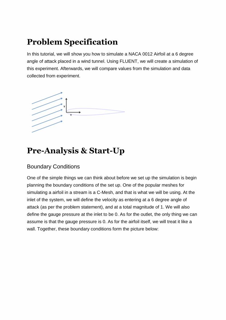
In this tutorial, we will show you how to simulate a NACA 0012 Airfoil at a 6 degree

angle of attack placed in a wind tunnel. Using FLUENT, we will create a simulation of

this experiment. Afterwards, we will compare values from the simulation and data

collected from experiment.

Pre-Analysis & Start-Up

Boundary Conditions

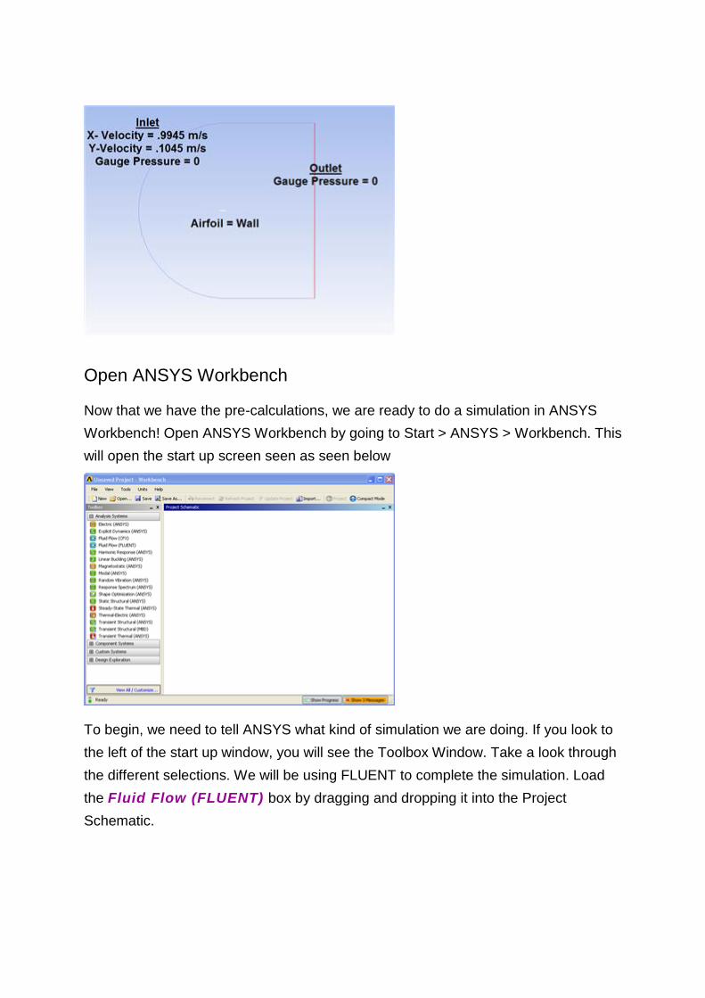
One of the simple things we can think about before we set up the simulation is begin

planning the boundary conditions of the set up. One of the popular meshes for

simulating a airfoil in a stream is a C-Mesh, and that is what we will be using. At the

inlet of the system, we will define the velocity as entering at a 6 degree angle of

attack (as per the problem statement), and at a total magnitude of 1. We will also

define the gauge pressure at the inlet to be 0. As for the outlet, the only thing we can

assume is that the gauge pressure is 0. As for the airfoil itself, we will treat it like a

wall. Together, these boundary conditions form the picture below:

Open ANSYS Workbench

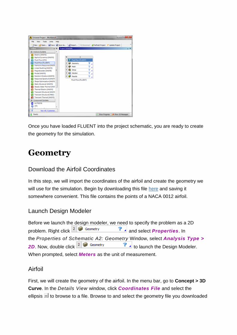
Now that we have the pre-calculations, we are ready to do a simulation in ANSYS

Workbench! Open ANSYS Workbench by going to Start > ANSYS > Workbench. This

will open the start up screen seen as seen below

To begin, we need to tell ANSYS what kind of simulation we are doing. If you look to

the left of the start up window, you will see the Toolbox Window. Take a look through

the different selections. We will be using FLUENT to complete the simulation. Load

the Fluid Flow (FLUENT) box by dragging and dropping it into the Project

Schematic.

Once you have loaded FLUENT into the project schematic, you are ready to create

the geometry for the simulation.

Geometry

Download the Airfoil Coordinates

In this step, we will import the coordinates of the airfoil and create the geometry we

will use for the simulation. Begin by downloading this file here and saving it

somewhere convenient. This file contains the points of a NACA 0012 airfoil.

Launch Design Modeler

Before we launch the design modeler, we need to specify the problem as a 2D

problem. Right click and select Properties. In

the Properties of Schematic A2: Geometry Window, select Analysis Type >

2D. Now, double click to launch the Design Modeler.

When prompted, select Meters as the unit of measurement.

Airfoil

First, we will create the geometry of the airfoil. In the menu bar, go to Concept > 3D

Curve. In the Details View window, click Coordinates File and select the

ellipsis to browse to a file. Browse to and select the geometry file you downloaded

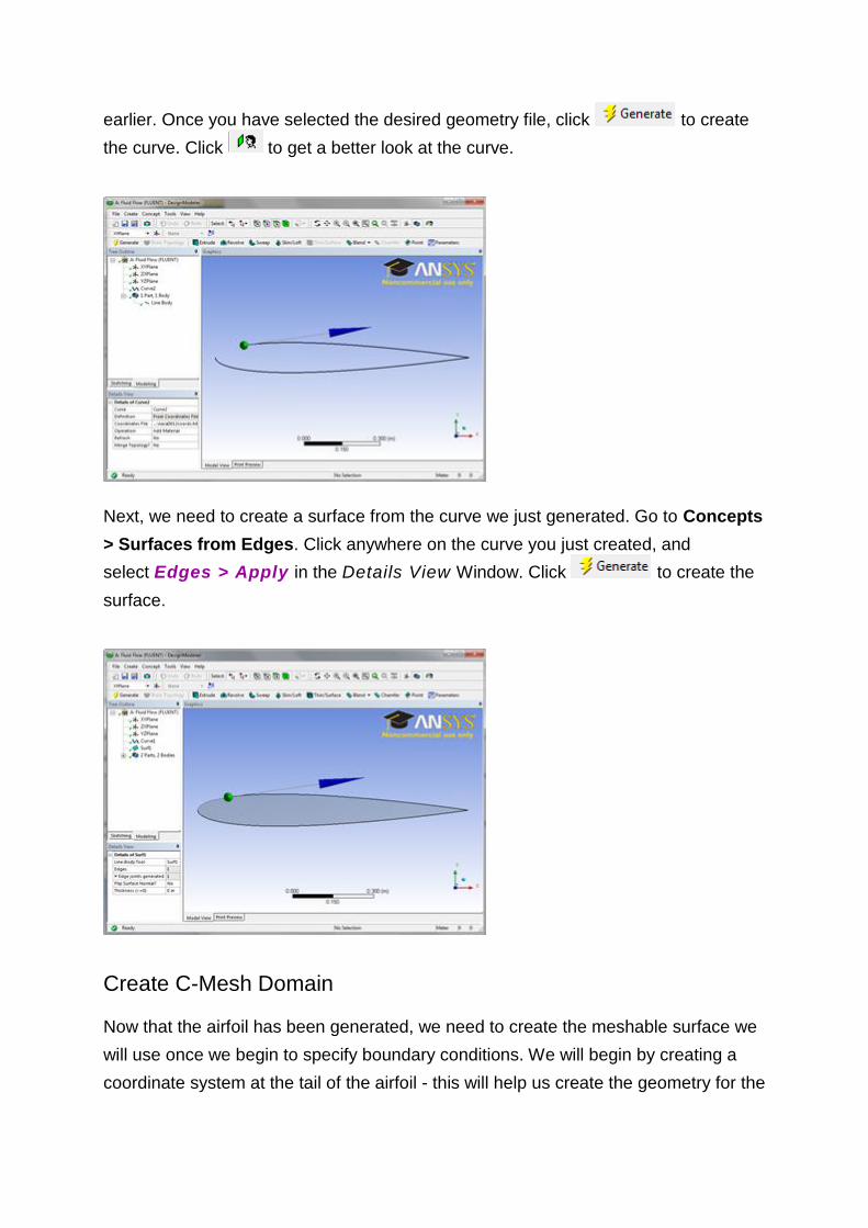
earlier. Once you have selected the desired geometry file, click to create

the curve. Click to get a better look at the curve.

Next, we need to create a surface from the curve we just generated. Go to Concepts

> Surfaces from Edges. Click anywhere on the curve you just created, and

select Edges > Apply in the Details View Window. Click to create the

surface.

Create C-Mesh Domain

Now that the airfoil has been generated, we need to create the meshable surface we

will use once we begin to specify boundary conditions. We will begin by creating a

coordinate system at the tail of the airfoil - this will help us create the geometry for the

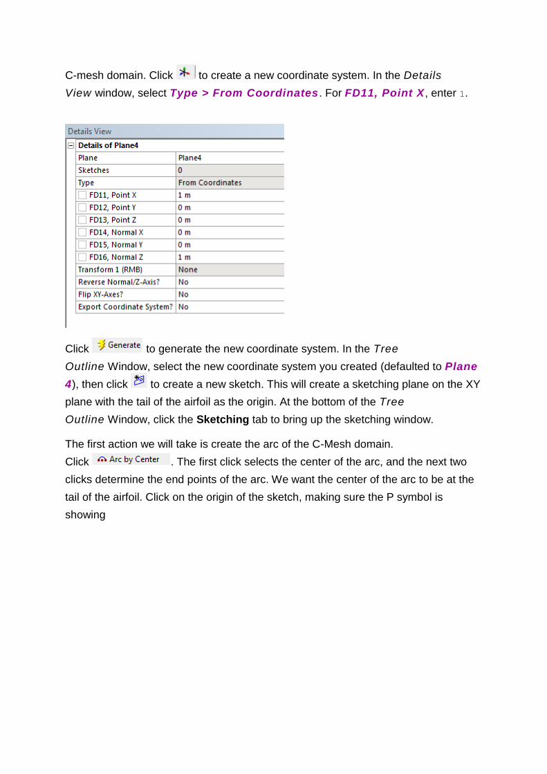
C-mesh domain. Click to create a new coordinate system. In the Details

View window, select Type > From Coordinates . For FD11, Point X, enter 1.

Click to generate the new coordinate system. In the Tree

Outline Window, select the new coordinate system you created (defaulted to Plane

4), then click to create a new sketch. This will create a sketching plane on the XY

plane with the tail of the airfoil as the origin. At the bottom of the Tree

Outline Window, click the Sketching tab to bring up the sketching window.

The first action we will take is create the arc of the C-Mesh domain.

Click . The first click selects the center of the arc, and the next two

clicks determine the end points of the arc. We want the center of the arc to be at the

tail of the airfoil. Click on the origin of the sketch, making sure the P symbol is

showing

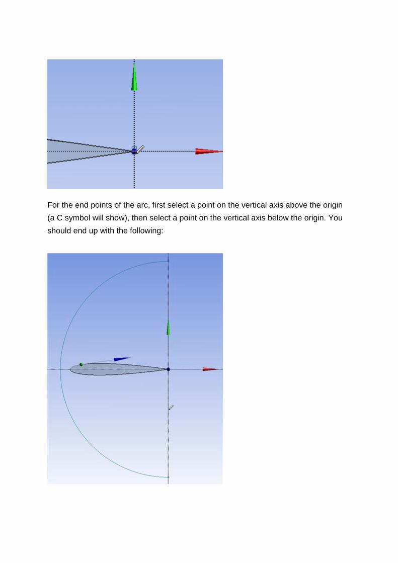
For the end points of the arc, first select a point on the vertical axis above the origin

(a C symbol will show), then select a point on the vertical axis below the origin. You

should end up with the following:

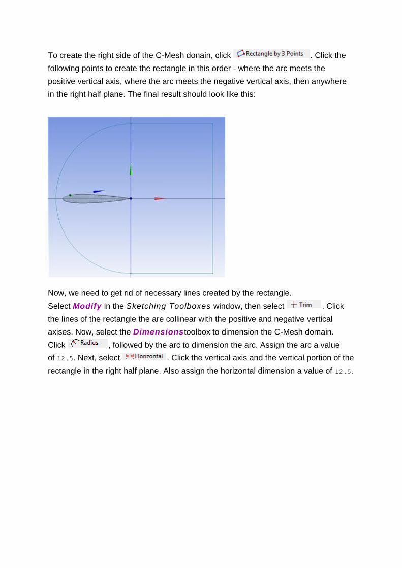
To create the right side of the C-Mesh donain, click . Click the

following points to create the rectangle in this order - where the arc meets the

positive vertical axis, where the arc meets the negative vertical axis, then anywhere

in the right half plane. The final result should look like this:

Now, we need to get rid of necessary lines created by the rectangle.

Select Modify in the Sketching Toolboxes window, then select . Click

the lines of the rectangle the are collinear with the positive and negative vertical

axises. Now, select the Dimensionstoolbox to dimension the C-Mesh domain.

Click , followed by the arc to dimension the arc. Assign the arc a value

of 12.5. Next, select . Click the vertical axis and the vertical portion of the

rectangle in the right half plane. Also assign the horizontal dimension a value of 12.5.

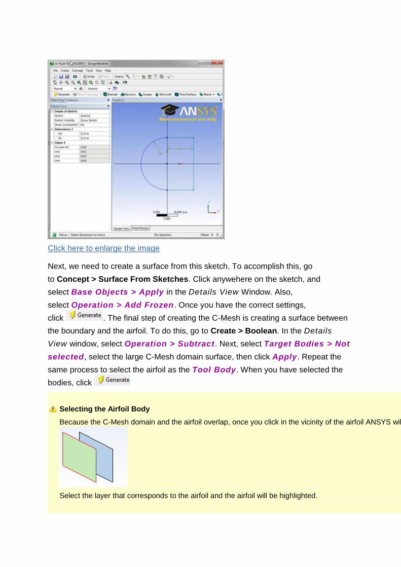
Click here to enlarge the image

Next, we need to create a surface from this sketch. To accomplish this, go

to Concept > Surface From Sketches. Click anywehere on the sketch, and

select Base Objects > Apply in the Details View Window. Also,

select Operation > Add Frozen. Once you have the correct settings,

click . The final step of creating the C-Mesh is creating a surface between

the boundary and the airfoil. To do this, go to Create > Boolean. In the Details

View window, select Operation > Subtract. Next, select Target Bodies > Not

selected, select the large C-Mesh domain surface, then click Apply. Repeat the

same process to select the airfoil as the Tool Body. When you have selected the

bodies, click

Selecting the Airfoil Body

Because the C-Mesh domain and the airfoil overlap, once you click in the vicinity of the airfoil ANSYS will select the C-Mesh domain but give you the option of selecting multiple layers

Select the layer that corresponds to the airfoil and the airfoil will be highlighted.

Create Quadrants

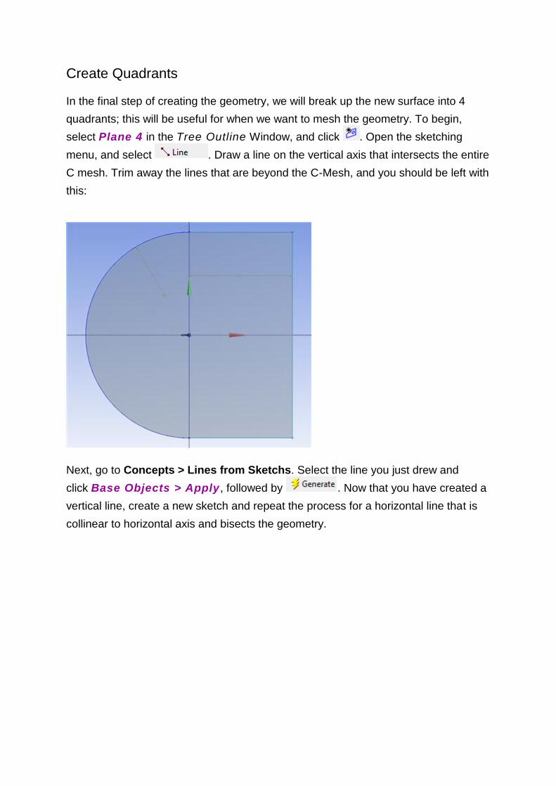
In the final step of creating the geometry, we will break up the new surface into 4

quadrants; this will be useful for when we want to mesh the geometry. To begin,

select Plane 4 in the Tree Outline Window, and click . Open the sketching

menu, and select . Draw a line on the vertical axis that intersects the entire

C mesh. Trim away the lines that are beyond the C-Mesh, and you should be left with

this:

Next, go to Concepts > Lines from Sketchs. Select the line you just drew and

click Base Objects > Apply , followed by . Now that you have created a

vertical line, create a new sketch and repeat the process for a horizontal line that is

collinear to horizontal axis and bisects the geometry.

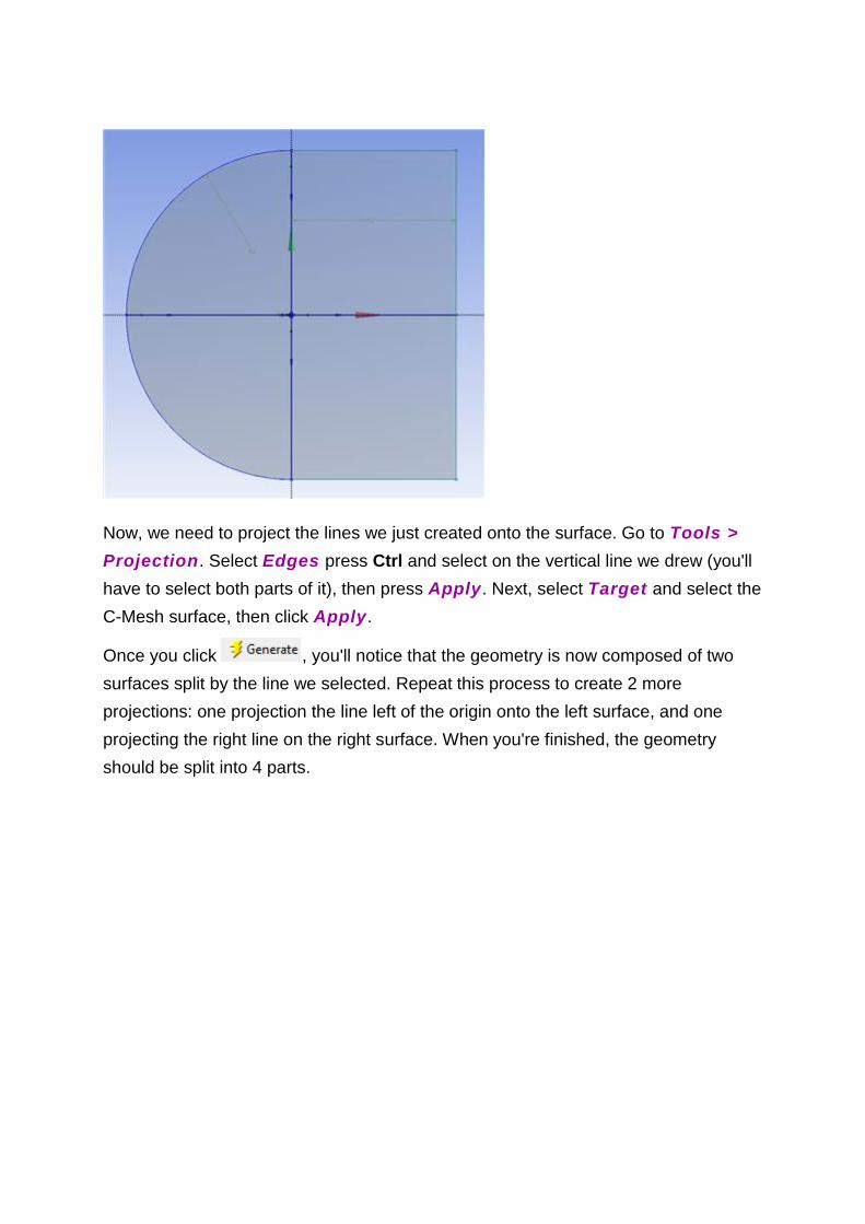
Now, we need to project the lines we just created onto the surface. Go to Tools >

Projection. Select Edges press Ctrl and select on the vertical line we drew (you'll

have to select both parts of it), then press Apply. Next, select Target and select the

C-Mesh surface, then click Apply.

Once you click , you'll notice that the geometry is now composed of two

surfaces split by the line we selected. Repeat this process to create 2 more

projections: one projection the line left of the origin onto the left surface, and one

projecting the right line on the right surface. When you're finished, the geometry

should be split into 4 parts.

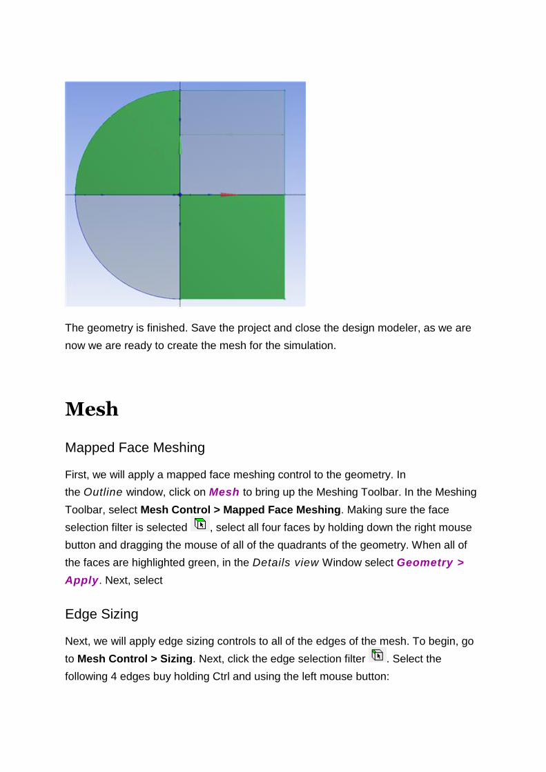
The geometry is finished. Save the project and close the design modeler, as we are

now we are ready to create the mesh for the simulation.

Mesh

Mapped Face Meshing

First, we will apply a mapped face meshing control to the geometry. In

the Outline window, click on Mesh to bring up the Meshing Toolbar. In the Meshing

Toolbar, select Mesh Control > Mapped Face Meshing. Making sure the face

selection filter is selected , select all four faces by holding down the right mouse

button and dragging the mouse of all of the quadrants of the geometry. When all of

the faces are highlighted green, in the Details view Window select Geometry >

Apply. Next, select

Edge Sizing

Next, we will apply edge sizing controls to all of the edges of the mesh. To begin, go

to Mesh Control > Sizing. Next, click the edge selection filter . Select the

following 4 edges buy holding Ctrl and using the left mouse button:

Click here to enlarge

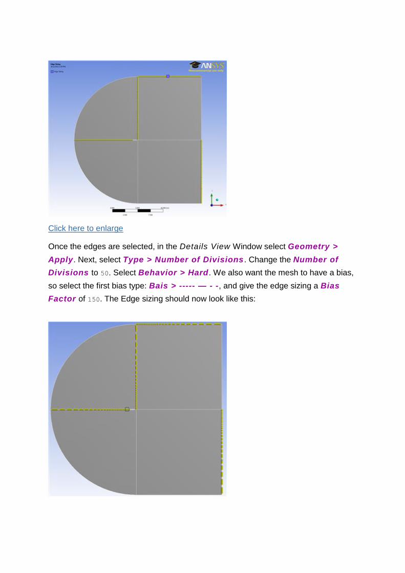
Once the edges are selected, in the Details View Window select Geometry >

Apply. Next, select Type > Number of Divisions . Change the Number of

Divisions to 50. Select Behavior > Hard. We also want the mesh to have a bias,

so select the first bias type: Bais > ----- — - -, and give the edge sizing a Bias

Factor of 150. The Edge sizing should now look like this:

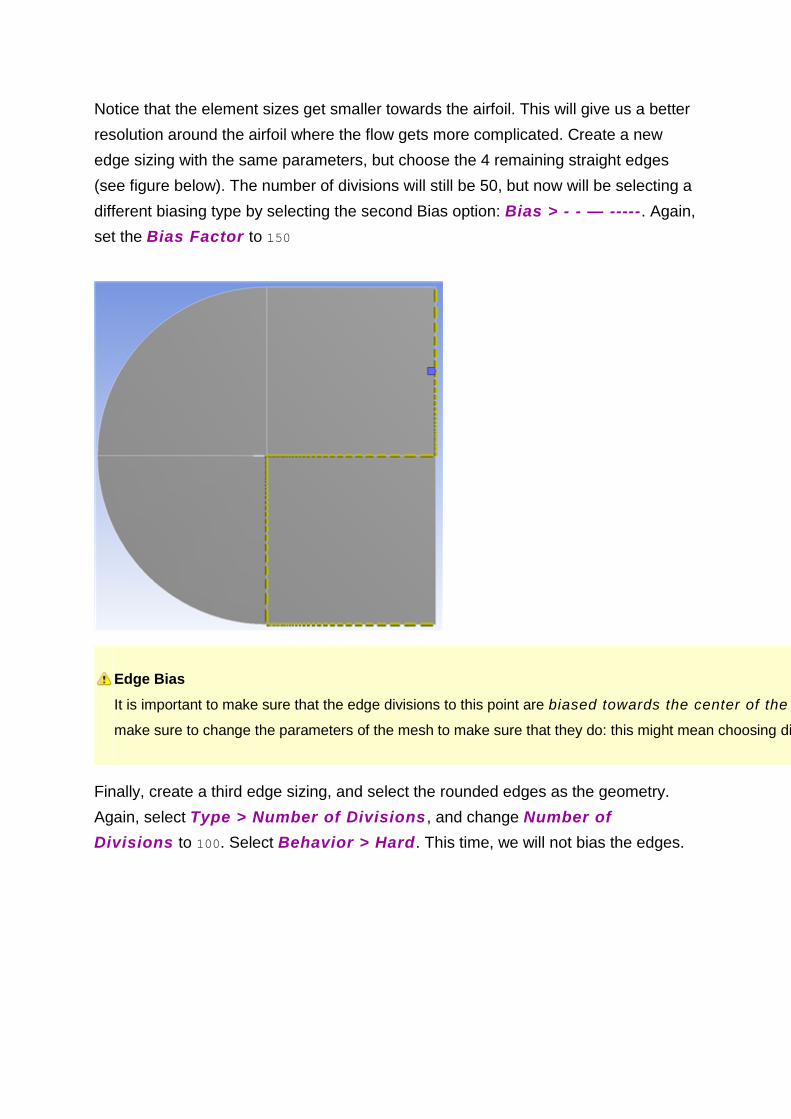
Notice that the element sizes get smaller towards the airfoil. This will give us a better

resolution around the airfoil where the flow gets more complicated. Create a new

edge sizing with the same parameters, but choose the 4 remaining straight edges

(see figure below). The number of divisions will still be 50, but now will be selecting a

different biasing type by selecting the second Bias option: Bias > - - — -----. Again,

set the Bias Factor to 150

Edge Bias

It is important to make sure that the edge divisions to this point are biased towards the center of the mesh : otherwise you may run into some problems later. If your mesh does not match the pictures in the tutorial,

make sure to change the parameters of the mesh to make sure that they do: this might mean choosing different edges for the different biasing types than those outlined in this tutorial.

Finally, create a third edge sizing, and select the rounded edges as the geometry.

Again, select Type > Number of Divisions , and change Number of

Divisions to 100. Select Behavior > Hard. This time, we will not bias the edges.

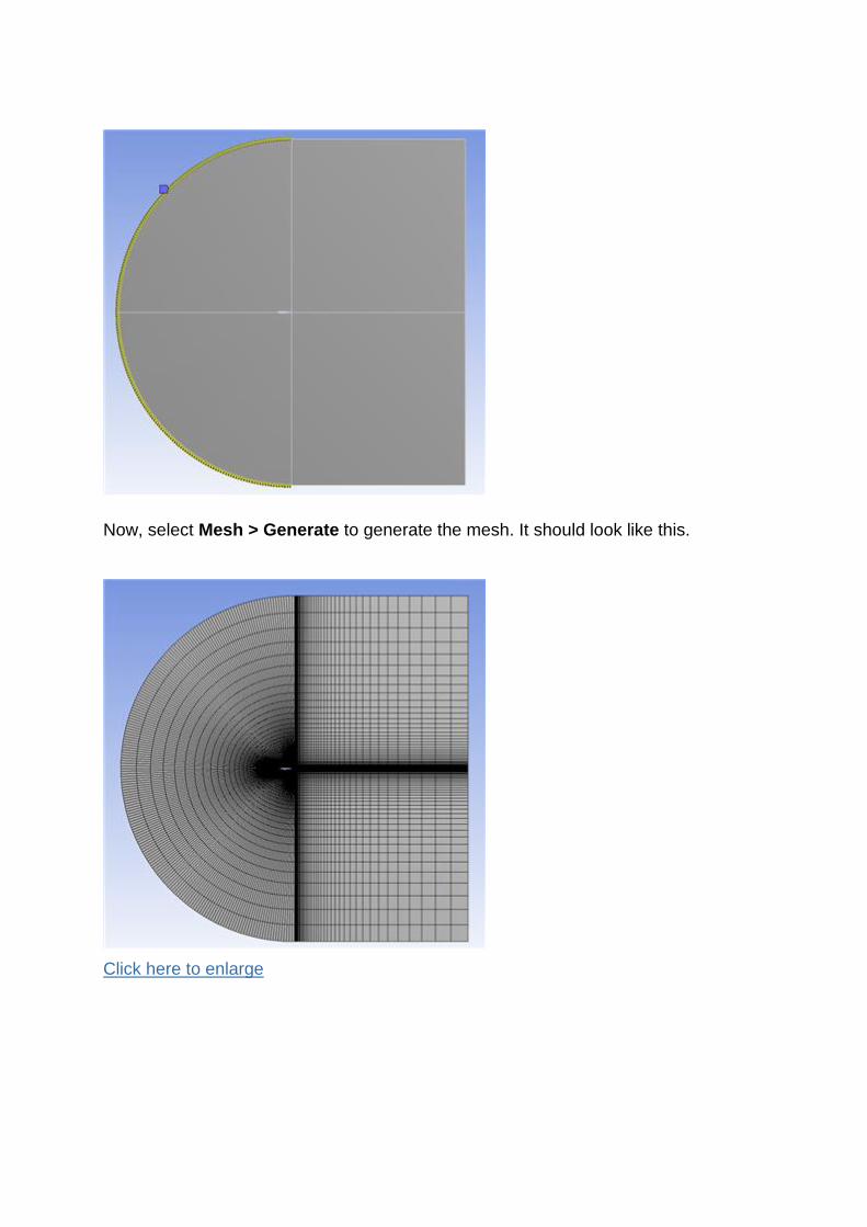
Now, select Mesh > Generate to generate the mesh. It should look like this.

Click here to enlarge

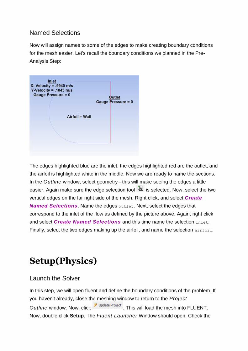
Named Selections

Now will assign names to some of the edges to make creating boundary conditions

for the mesh easier. Let's recall the boundary conditions we planned in the Pre-

Analysis Step:

The edges highlighted blue are the inlet, the edges highlighted red are the outlet, and

the airfoil is highlighted white in the middle. Now we are ready to name the sections.

In the Outline window, select geometry - this will make seeing the edges a little

easier. Again make sure the edge selection tool is selected. Now, select the two

vertical edges on the far right side of the mesh. Right click, and select Create

Named Selections. Name the edges outlet. Next, select the edges that

correspond to the inlet of the flow as defined by the picture above. Again, right click

and select Create Named Selections and this time name the selection inlet.

Finally, select the two edges making up the airfoil, and name the selection airfoil.

Setup(Physics)

Launch the Solver

In this step, we will open fluent and define the boundary conditions of the problem. If

you haven't already, close the meshing window to return to the Project

Outline window. Now, click . This will load the mesh into FLUENT.

Now, double click Setup. The Fluent Launcher Window should open. Check the

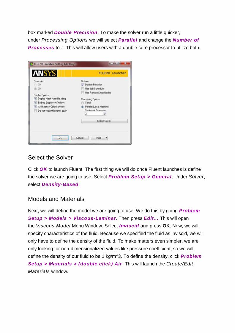
box marked Double Precision. To make the solver run a little quicker,

under Processing Options we will select Parallel and change the Number of

Processes to 2. This will allow users with a double core processor to utilize both.

Select the Solver

Click OK to launch Fluent. The first thing we will do once Fluent launches is define

the solver we are going to use. Select Problem Setup > General . Under Solver,

select Density-Based.

Models and Materials

Next, we will define the model we are going to use. We do this by going Problem

Setup > Models > Viscous-Laminar. Then press Edit... This will open

the Viscous Model Menu Window. Select Inviscid and press OK. Now, we will

specify characteristics of the fluid. Because we specified the fluid as inviscid, we will

only have to define the density of the fluid. To make matters even simpler, we are

only looking for non-dimensionalized values like pressure coefficient, so we will

define the density of our fluid to be 1 kg/m^3. To define the density, click Problem

Setup > Materials > (double click) Air . This will launch the Create/Edit

Materials window.

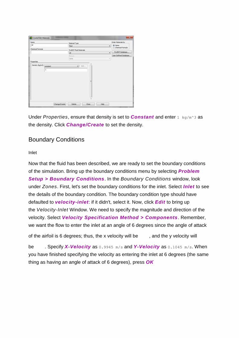
Under Properties, ensure that density is set to Constant and enter 1 kg/m^3 as

the density. Click Change/Create to set the density.

Boundary Conditions

Inlet

Now that the fluid has been described, we are ready to set the boundary conditions

of the simulation. Bring up the boundary conditions menu by selecting Problem

Setup > Boundary Conditions . In the Boundary Conditions window, look

under Zones. First, let's set the boundary conditions for the inlet. Select Inlet to see

the details of the boundary condition. The boundary condition type should have

defaulted to velocity-inlet: if it didn't, select it. Now, click Edit to bring up

the Velocity-Inlet Window. We need to specify the magnitude and direction of the

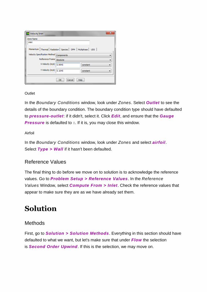
velocity. Select Velocity Specification Method > Components . Remember,

we want the flow to enter the inlet at an angle of 6 degrees since the angle of attack

of the airfoil is 6 degrees; thus, the x velocity will be , and the y velocity will

be . Specify X-Velocity as 0.9945 m/s and Y-Velocity as 0.1045 m/s. When

you have finished specifying the velocity as entering the inlet at 6 degrees (the same

thing as having an angle of attack of 6 degrees), press OK

Outlet

In the Boundary Conditions window, look under Zones. Select Outlet to see the

details of the boundary condition. The boundary condition type should have defaulted

to pressure-outlet: if it didn't, select it. Click Edit, and ensure that the Gauge

Pressure is defaulted to 0. If it is, you may close this window.

Airfoil

In the Boundary Conditions window, look under Zones and select airfoil.

Select Type > Wall if it hasn't been defaulted.

Reference Values

The final thing to do before we move on to solution is to acknowledge the reference

values. Go to Problem Setup > Reference Values. In the Reference

Values Window, select Compute From > Inlet. Check the reference values that

appear to make sure they are as we have already set them.

Solution

Methods

First, go to Solution > Solution Methods . Everything in this section should have

defaulted to what we want, but let's make sure that under Flow the selection

is Second Order Upwind. If this is the selection, we may move on.

Monitors

Now we are ready to begin solving the simulation. Before we hit solve though, we

need to set up some parameters for how Fluent will solve the simulation.

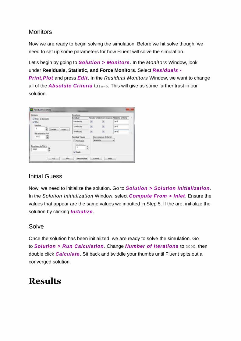
Let's begin by going to Solution > Monitors . In the Monitors Window, look

under Residuals, Statistic, and Force Monitors. Select Residuals -

Print,Plot and press Edit. In the Residual Monitors Window, we want to change

all of the Absolute Criteria to1e-6. This will give us some further trust in our

solution.

Initial Guess

Now, we need to initialize the solution. Go to Solution > Solution Initialization .

In the Solution Initialization Window, select Compute From > Inlet. Ensure the

values that appear are the same values we inputted in Step 5. If the are, initialize the

solution by clicking Initialize.

Solve

Once the solution has been initialized, we are ready to solve the simulation. Go

to Solution > Run Calculation . Change Number of Iterations to 3000, then

double click Calculate. Sit back and twiddle your thumbs until Fluent spits out a

converged solution.

Results

Velocity

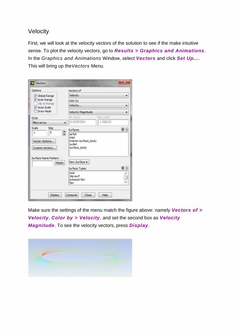
First, we will look at the velocity vectors of the solution to see if the make intuitive

sense. To plot the velocity vectors, go to Results > Graphics and Animations .

In the Graphics and Animations Window, select Vectors and click Set Up....

This will bring up theVectors Menu.

Make sure the settings of the menu match the figure above: namely Vectors of >

Velocity, Color by > Velocity , and set the second box as Velocity

Magnitude. To see the velocity vectors, press Display.

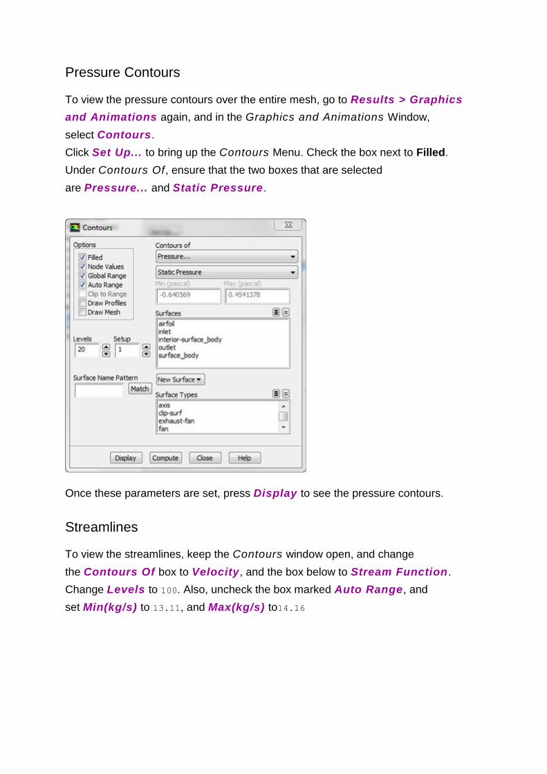
Pressure Contours

To view the pressure contours over the entire mesh, go to Results > Graphics

and Animations again, and in the Graphics and Animations Window,

select Contours.

Click Set Up... to bring up the Contours Menu. Check the box next to Filled.

Under Contours Of, ensure that the two boxes that are selected

are Pressure... and Static Pressure.

Once these parameters are set, press Display to see the pressure contours.

Streamlines

To view the streamlines, keep the Contours window open, and change

the Contours Of box to Velocity, and the box below to Stream Function.

Change Levels to 100. Also, uncheck the box marked Auto Range, and

set Min(kg/s) to 13.11, and Max(kg/s) to14.16

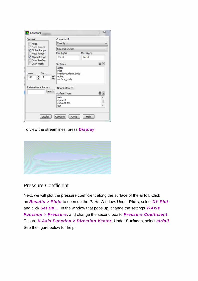
To view the streamlines, press Display

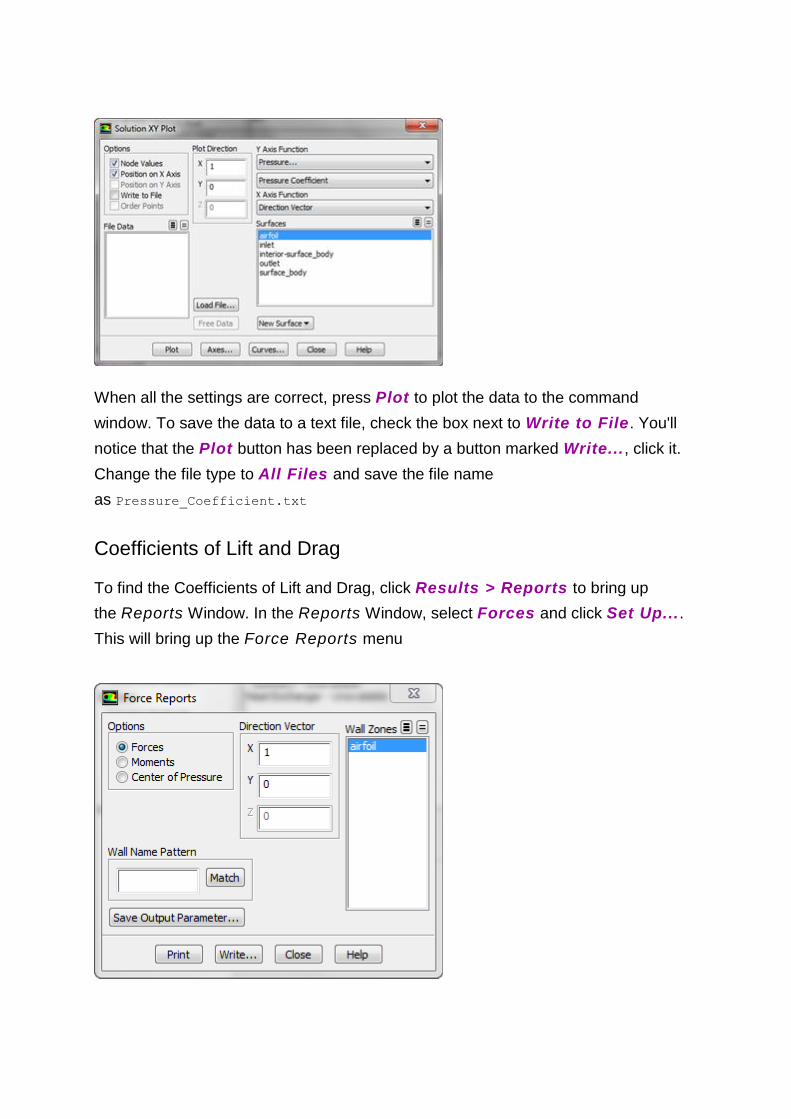
Pressure Coefficient

Next, we will plot the pressure coefficient along the surface of the airfoil. Click

on Results > Plots to open up the Plots Window. Under Plots, select XY Plot,

and click Set Up.... In the window that pops up, change the settings Y-Axis

Function > Pressure , and change the second box to Pressure Coefficient.

Ensure X-Axis Function > Direction Vector . Under Surfaces, select airfoil.

See the figure below for help.

When all the settings are correct, press Plot to plot the data to the command

window. To save the data to a text file, check the box next to Write to File. You'll

notice that the Plot button has been replaced by a button marked Write..., click it.

Change the file type to All Files and save the file name

as Pressure_Coefficient.txt

Coefficients of Lift and Drag

To find the Coefficients of Lift and Drag, click Results > Reports to bring up

the Reports Window. In the Reports Window, select Forces and click Set Up....

This will bring up the Force Reports menu

We need to set the parameters so drag across the airfoil (keep in mind, which is at an

angle) will be displayed. In the Force Reports window change the Direction

Vector such that X > .9945 and Y > .1045. Click Print to print the drag coefficient

to the command window. To print the lift coefficient, in the Force Reports window

change the Direction Vector such that X > -.1045 and Y > .9945. Again,

press Print.

Verification and Validation

Verification

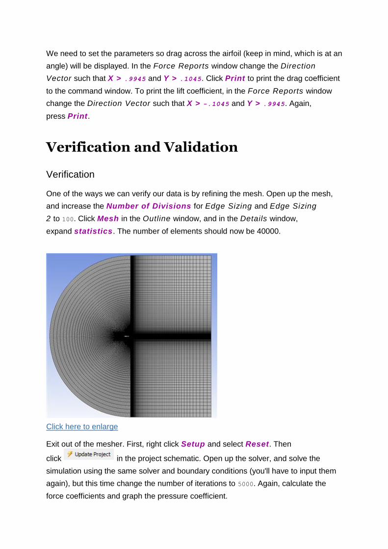
One of the ways we can verify our data is by refining the mesh. Open up the mesh,

and increase the Number of Divisions for Edge Sizing and Edge Sizing

2 to 100. Click Mesh in the Outline window, and in the Details window,

expand statistics. The number of elements should now be 40000.

Click here to enlarge

Exit out of the mesher. First, right click Setup and select Reset. Then

click in the project schematic. Open up the solver, and solve the

simulation using the same solver and boundary conditions (you'll have to input them

again), but this time change the number of iterations to 5000. Again, calculate the

force coefficients and graph the pressure coefficient.

Validation

To validate our data, we will take a compare the data from actual experiment.

Unrefined Mesh Refined Mesh Experimental Data

Lift Coeffient 0.6315 0.6670 0.6630

Drag Coefficient 0.0122 0.0063 0.0090

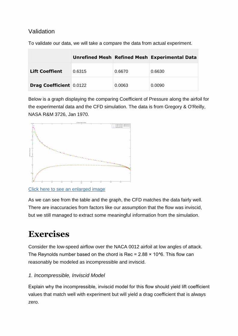
Below is a graph displaying the comparing Coefficient of Pressure along the airfoil for

the experimental data and the CFD simulation. The data is from Gregory & O'Reilly,

NASA R&M 3726, Jan 1970.

Click here to see an enlarged image

As we can see from the table and the graph, the CFD matches the data fairly well.

There are inaccuracies from factors like our assumption that the flow was inviscid,

but we still managed to extract some meaningful information from the simulation.

Exercises

Consider the low-speed airflow over the NACA 0012 airfoil at low angles of attack.

The Reynolds number based on the chord is Rec = 2.88 × 10^6. This flow can

reasonably be modeled as incompressible and inviscid.

1. Incompressible, Inviscid Model

Explain why the incompressible, inviscid model for this flow should yield lift coefficient

values that match well with experiment but will yield a drag coefficient that is always

zero.

2. Boundary Value Problem

What is the boundary value problem (BVP) you need to solve to obtain the velocity

and pressure distributions for this flow at an angle of attack of 10 degrees? Indicate

governing equations, domain and boundary conditions (u = 0 at a certain boundary

etc.). For each of the boundary conditions, indicate also the corresponding boundary

type that you need to select in FLUENT.

3. Coefficient of Pressure

Run a simulation for the NACA 0012 airfoil at angles of attack at 0 degrees and 10

degrees for two cases: a mesh with 15000 elements and a mesh with 40000

elements. Plot the pressure coefficient obtained from FLUENT on the same plot as

data obtained from experiment The experimental data is from Gregory & O’Reilly,

NASA R&M 3726, Jan 1970 and is provided here Follow the aeronautical convention

of flipping the vertical axis so that negative Cp values are above and positive Cp

values are below. This can be done in MATLAB using set(gca, ’YDir’, ’reverse’);

4. Lift and Drag Coefficient

Obtain the lift and drag coefficients from the FLUENT results on the two meshes.

Compare these with experimental or expected values (present this comparison as a

table). The experimental values for 0 degree angle of attack are: Cl = 0.025; Cd =

0.0069, and the experimental values for 10 degree angle of attack are: Cl = 1.2219;

Cd = 0.0138.

Conclusions

Comment on the comparison with experiment for the two angles of attack.

Also,comment on the effect of mesh refinement. How does the pressure distribution

over the airfoil change on increasing the angle of attack?