al metho d) 27 - mayo

An Introduction to Recursive Partitioning

Using the RPART Routines

Elizabeth J. Atkinson

Terry M. Therneau

Mayo Foundation

February 11, 2000

Contents

1 Introduction 3

2 Basic steps needed to use rpart 3

3 Rpart model options 4

4 Plotting options 6

4.1 plot.rpart options : : : : : : : : : : : : : : : : : : : : : : : : : : : : : 6

4.2 text.rpart options : : : : : : : : : : : : : : : : : : : : : : : : : : : : : 7

4.3 Examples using plot.rpart and text.rpart together : : : : : : : : : : 8

5 Other available functions 12

6 Examples with explanation of output 13

6.1 Stage C prostate cancer (class method) : : : : : : : : : : : : : : : : 13

6.1.1 print function : : : : : : : : : : : : : : : : : : : : : : : : : : : 14

6.1.2 printcp function : : : : : : : : : : : : : : : : : : : : : : : : : 15

6.1.3 summary function : : : : : : : : : : : : : : : : : : : : : : : : 16

6.2 Consumer Report Auto data (anova method) : : : : : : : : : : : : : 18

6.2.1 print, printcp functions : : : : : : : : : : : : : : : : : : : : : 19


6.2.3 plot, text, rsq.rpart functions : : : : : : : : : : : : : : : : : : 22

6.3 Solder data (poisson method) : : : : : : : : : : : : : : : : : : : : : : 23

6.3.1 print function : : : : : : : : : : : : : : : : : : : : : : : : : : : 25

1


6.3.3 plot, text, prune functions : : : : : : : : : : : : : : : : : : : : 27

6.4 Stage C Prostate cancer (survival method) : : : : : : : : : : : : : : : 27

2

1 Introduction

This document is a shortened version of the Mayo Clinic Section of Biostatistics

technical report [5] written by Terry Therneau and Beth Atkinson. More complete

information about the theory behind the coding can be obtained there. The follow-

ing pages provide an overview of the methods found in the rpart routines, which

implement many of the ideas found in the CART (Classi�cation and Regression

Trees) book and programs of Breiman, Friedman, Olshen and Stone [1]. Because

CART is the trademarked name of a particular software implementation of these

ideas, and tree has been used for the S-plus routines of Clark and Pregibon�[2] a

di�erent acronym | Recursive PARTitioning or rpart | was chosen.

The rpart programs build classi�cation or regression models of a very general

structure using a two stage procedure; the resulting models can be represented as

binary trees. The types of endpoints that rpart handles includes classi�cations

(such as yes/no), continuous values (such as bone mineral density), poisson counts

(such as the number of fractures in Medicare patients), and survival information

(time to death/last known contact). The rpart library includes tools to model,

plot, and summarize the end results.

2 Basic steps needed to use rpart

Step{I. Attach the library so that the functions can be found.

library(rpart)

Step{II. Decide what type of endpoint you have

� Categorical ==> method == "class"

� Continuous ==> method == "anova"

� Poisson Process/Count ==> method == "poisson"

� Survival ==> method == "exp"

Step{III. Fit the model using the standard Splus modeling language.

fit <- rpart(skips ~ Opening + Solder + Mask + PadType

+ Panel, data=solder, method='poisson')

Step{IV. Print a text version of the tree.

print(fit)

Step{V. Print a summary which examines each node in depth.

3

summary(fit)

Step{VI. Plot a standard version of the plot with some basic information.

plot(fit)

text(fit,use.n=T)

Step{VII. Create a prettier version of the tree.

post(fit,file="")

3 Rpart model options

This section examines the various options that are available when �tting the model

rpart. The options are listed below with a brief explanation, then explored further

with actual examples.

The central �tting function is rpart, whose main arguments are

formula: the model formula, as in lm and other S model �tting functions. The

right hand side may contain both continuous and categorical (factor) terms.

If the outcome y has more than two levels, then categorical predictors must

be �t by exhaustive enumeration, which can take a very long time.

data, weights, subset: as for other S models.

method: the type of splitting rule to use. Options at this point are classi�cation,

anova, Poisson, and exponential.

parms: a list of method speci�c optional parameters. Poisson splitting has a single

parameter, the coe�cient of variation of the prior distribution on the rates

(shrink). It is used to prevent problems if nodes end up with 0 events. Usually

not changed (default=1). For classi�cation, the list can contain any of:

� prior{ the vector of prior probabilities

� loss{ the loss matrix

� split{ the splitting index

The priors must be positive and sum to 1. The loss matrix must have zeros

on the diagonal and positive o�-diagonal elements. The splitting index can be

`gini' or `information'.

4

> lmat <- matrix(c(0,4,3,0), nrow=2, ncol=2, byrow=F)

> fit1 <- rpart(Kyphosis ~ Age + Number + Start, data=kyphosis,loss

method='class', parms=list(split='gini', loss=lmat, shrink=0))

> fit2 <- rpart(Kyphosis ~ Age + Number + Start, data=kyphosis,

method='class', parms=list(split='gini', prior=

c(.65,.35)))

> wts <- rep(3, nrow(stagec))

> fit3 <- rpart(Surv(pgtime, pgstat) ~ age + eet + g2+grade+gleason +ploidy,

stagec, parms=list(shrink=0), method="poisson", weights=wts)

na.action: the action for missing values. The default action for rpart is na.rpart,

this default is not overridden by the options(na.action) global option. The

default action removes only those rows for which either the response y or all of

the predictors are missing. This ability to retain partially missing observations

is perhaps the single most useful feature of rpart models.

control: a list of control parameters, usually the result of the rpart.control func-

tion. The list contains

� minsplit: The minimum number of observations in a node for which

the routine will even try to compute a split. The default is 20. This

parameter can save computation time, since smaller nodes are almost

always pruned away by cross-validation.

� minbucket: The minimum number of observations in a terminal node.

This defaults to minsplit/3.

� maxcompete: It is often useful in the printout to see not only the variable

that gave the best split at a node, but also the second, third, etc best.

This parameter controls the number that will be printed. It has no e�ect

on computational time, and a small e�ect on the amount of memory used.

The default is 5.

� xval: The number of cross-validations to be done. Usually set to zero

during exploritory phases of the analysis. A value of 10, for instance,

increases the compute time to 11-fold over a value of 0.

� maxsurrogate: The maximum number of surrogate variables to retain at

each node. (No surrogate that does worse than \go with the majority"

is printed or used). Setting this to zero will cut the computation time

in half, and set usesurrogate to zero. The default is 5. Surrogates give

di�erent information than competitor splits. The competitor list asks

\which other splits would have as many correct classi�cations", surro-

gates ask \which other splits would classify the same subjects in the

same way", which is a harsher criteria.

5

� usesurrogate: A value of usesurrogate=2, the default, splits subjects in

the way described previously. This is similar to CART. If the value is 0,

then a subject who is missing the primary split variable does not progress

further down the tree. A value of 1 is intermediate: all surrogate variables

except \go with the majority" are used to send a case further down the

tree.

� cp: The threshold complexity parameter.

> temp <- rpart.control(xval=10, minbucket=2, minsplit=4, cp=0)

> dfit <- rpart(y � x, method='class', control=temp)

4 Plotting options

This section examines the various options that are available when plotting an rpart

object. The options are listed below with a brief explanation, then explored further

with actual plots.

4.1 plot.rpart options

The function plot.rpart plots an rpart object on the current graphics device. The

main arguments to the function are

Required Arguments: arguments you must specify.

tree: a �tted object of class rpart, containing a classi�cation, regression, or

rate tree.

Optional Arguments: arguments you can add if you wish.

uniform: if TRUE, uniform vertical spacing of the nodes is used; this may

be less cluttered when �tting a large plot onto a page. The default is to

use a non-uniform spacing proportional to the error in the �t.

branch: controls the shape of the branches from parent to child node. Any

number from 0 to 1 is allowed. A value of 1 gives square shouldered

branches, a value of 0 give V shaped branches, with other values being

intermediate.

compress: if FALSE, the leaf nodes will be at the horzontal plot coordi-

nates of 1:nleaves (like plot.tree). If TRUE, the routine attempts a more

compact arrangement of the tree. The compaction algorithm assumes

uniform=T.

6

nspace: the amount of extra space between a node with children and a leaf,

as compared to the minimal space between leaves. Applies to compressed

trees only. The default is the value of branch.

margin: an extra percentage of white space to leave around the borders of

the tree. (Long labels sometimes get cut o� by the default computation).

minbranch: set the minimum length for a branch to minbranch times the av-

erage branch length. This parameter is ignored if uniform=T. Sometimes

a split will give very little improvement, or even (in the classi�cation case)

no improvement at all. A tree with branch lengths strictly proportional

to improvement leaves no room to squeeze in node labels.

4.2 text.rpart options

The function text.rpart labels the current plot of the tree dendrogram with text.

The main arguments to this function are

Required Arguments: arguments you must specify.

x: �tted model object of class rpart. This is assumed to be the result of some

function that produces an object with the same named components as

that returned by the rpart function.

Optional Arguments: arguments you can add if you wish.

splits: logical ag. If TRUE (default), then the splits in the tree are labeled

with the criterion for the split.

label: a column name of x$frame; values of this will label the nodes.

FUN: the name of a labeling function, e.g. text.

all: Logical. If TRUE, all nodes are labeled, otherwise just terminal nodes.

pretty: an integer denoting the extent to which factor levels in split labels

will be abbreviated. A value of (0) signi�es no abbreviation. A NULL

(default) signi�es using elements of letters to represent the di�erent factor

levels.

digits: number of signi�cant digits to include in numerical labels.

use.n: Logical. If TRUE, adds to label (#events level1/ #events level2/etc.

for class, n for anova, and # events/n for poisson and exp).

fancy: Logical. If TRUE, nodes are represented by ellipses (interior nodes)

and rectangles (leaves) and labeled by yval. The edges connecting the

nodes are labeled by left and right splits.

7

|grade<2.5

g2<13.2

ploidy:ab

g2>11.845g2<11.005

g2>17.91

No

No

No Prog

Prog

No Prog

Figure 1: plot(fit); text(fit)

fwidth: Relates to option fancy and the width of the ellipses and rectangles.

If fwidth < 1 then it is a scaling factor (default = .8). If fwidth > 1

then it represents the number of character widths (for current graphical

device) to use.

fheight: Relates to option fancy and the height of the ellipses and rectangles.

If fheight < 1 then it is a scaling factor (default = .8). If fheight > 1

then it represents the number of character heights (for current graphical

device) to use.

4.3 Examples using plot.rpart and text.rpart together

For simplicity, the same model will be used throughout the subsection. The simpliest

labelled plot (�gure 1) is called by using plot and text without changing any of the

defaults. This is useful for a �rst look, but sometimes you'll want more information

about each of the nodes.

> fit <- rpart(progstat � age + eet + g2 + grade + gleason + ploidy,

stagec, control=rpart.control(cp=.025))

> plot(fit)

> text(fit)

8

|grade<2.5

g2<13.2

ploidy:ab

g2>11.845

g2<11.005

g2>17.91

No(92/54)

No(52/9)

Prog(40/45)

No(23/17)

No(20/11)

No(6/1)

No(14/10)

No(12/5)

Prog(2/5)

Prog(3/6)

Prog(17/28)

No(14/8)

Prog(3/20)

Figure 2: plot(fit, uniform=T); text(fit,use.n=T,all=T)

The next plot (�gure 2) has uniform stem lengths (uniform=T), has extra infor-

mation (use.n=T) specifying number of subjects at each node (here it lists how many

are diseased and how many are not diseased), and has labels on all the nodes, not

just the terminal nodes (all=T).

> plot(fit, uniform=T)

> text(fit, use.n=T, all=T)

Fancier plots can be created by modifying the branch option, which controls the

shape of branches that connect a node to its children. The default for the plots

is to have square shouldered trees (branch = 1.0). This can be taken to the other

extreme with no shoulders at all (branch=0) as shown in �gure 3.

> plot(fit, branch=0)

> text(fit, use.n=T)

These options can be combined with others to create the plot that �ts your

particular needs. The default plot may be ine�cient in it's use of space: the terminal

nodes will always lie at x-coordinates of 1,2,: : : . The compress option attempts to

improve this by overlapping some nodes. It has little e�ect on �gure 4, but in �gure

3 it allows the lowest branch to \tuck under" those above. If you want to play

around with the spacing with compress, try using nspace which regulates the space

between a terminal node and a split.

9

grade<2.5

g2<13.2

ploidy:ab

g2>11.845g2<11.005

g2>17.91

No(52/9)

No(6/1)

No(12/5)

Prog(2/5)

Prog(3/6)

No(14/8)

Prog(3/20)

Figure 3: plot(fit, branch=0); text(fit,use.n=T)

|grade<2.5

g2<13.2

ploidy:ab

g2>11.845

g2<11.005

g2>17.91

No(92/54)

No(52/9)

Prog(40/45)

No(23/17)

No(20/11)

No(6/1)

No(14/10)

No(12/5)

Prog(2/5)

Prog(3/6)

Prog(17/28)

No(14/8)

Prog(3/20)

Figure 4: plot(fit, branch=.4, uniform=T,compress=T)

10

|grade<2.5

g2<13.2

ploidy:d,t

g2>11.845

g2<11.005

g2>17.91

grade>2.5

g2>13.2

ploidy:a

g2<11.845

g2>11.005

g2<17.91

No(92/54)

No(52/9)

Prog(40/45)

No(23/17)

No(20/11)

No(6/1)

No(14/10)

No(12/5)

Prog(2/5)

Prog(3/6)

Prog(17/28)

No(14/8)

Prog(3/20)

Endpoint = progstat

Figure 5: post(fit)

> plot(fit,branch=.4,uniform=T,compress=T)

> text(fit,all=T,use.n=T)

We have combined several of these options into a function called post.rpart.

Results are shown in �gure 5. The code is essentially

> plot(tree, uniform = T, branch = 0.2, compress = T, margin = 0.1)

> text(tree, all = T, use.n=T, fancy = T)

The fancy option of text creates the ellipses and rectangles, and moves the splitting

rule to the midpoints of the branches. Margin shrinks the plotting region slightly so

that the text boxes don't run over the edge of the plot. The branch option makes

the lines exit the ellipse at a \good" angle. The call post(fit) will create a postcript

�le �t.ps in the current directory. The additional argument file="" will cause the

plot to appear on the current active device. Note that post.rpart is just our choice

of options to the functions plot.rpart and text.rpart. The reader is encouraged to

try out other possibilities, as these speci�cations may not be the best choice in all

situations.

11

5 Other available functions

There are a number of other functions in the rpart library. This list describes the

all the main rpart functions brie y. More details about the functions can be found

on the help pages in Splus (ex. help(snip.rpart)) or elsewhere in this document.

as.tree Create a tree object from an rpart object.

meanvar.rpart Mean-Variance plot for an rpart object.

rsq.rpart Plots R-square versus number of splits.

resid.rpart Residuals from an rpart object.

predict.rpart Predictions from an rpart object.

plot.rpart Plot an rpart object.

plotcp Plot the Complexity Parameter (cp) for an rpart object.

post.rpart Plot an rpart object - prettier version.

print.rpart Print a rpart object.

printcp Print the Complexity Parameter (cp) table for an rpart object.

prune.rpart Prune back an rpart object given a complexity parameter value rang-

ing from 0 to 1.

snip.rpart Snip subtrees of an rpart object.

summary.rpart Summarize an rpart object.

text.rpart Place text on a dendrogram.

xpred.rpart Cross-validation for rpart object.

There are also some tree functions that may work for rpart objects, once the

function as.tree has been applied to it. These functions are

hist.tree Augment a dendrogram with histograms.

rug.tree Augment a dendrogram with a rug.

tile.tree Augment a dendrogram with tiles.

12

|grade<2.5

g2<13.2

ploidy:ab

g2>11.845

g2<11.005

g2>17.91

age>62.5

No

No

No Prog

Prog

No ProgProg

Figure 6: Classi�cation tree for the Stage C data

6 Examples with explanation of output

6.1 Stage C prostate cancer (class method)

This �rst example is based on a data set of 146 stage C prostate cancer patients

[4]. The main clinical endpoint of interest is whether the disease recurs after initial

surgical removal of the prostate, and the time interval to that progression (if any).

The endpoint in this example is status, which takes on the value 1 if the disease

has progressed and 0 if not. Later we'll analyze the data using the exp method,

which will take into account time to progression. A short description of each of the

variables is listed below. The main predictor variable of interest in this study was

DNA ploidy, as determined by ow cytometry. For diploid and tetraploid tumors,

the ow cytometric method was also able to estimate the percent of tumor cells

in a G2 (growth) stage of their cell cycle; G2% is systematically missing for most

aneuploid tumors.

The variables in the data set are

13

pgtime time to progression, or last follow-up free of progression

pgstat status at last follow-up (1=progressed, 0=censored)

age age at diagnosis

eet early endocrine therapy (1=no, 0=yes)

ploidy diploid/tetraploid/aneuploid DNA pattern

g2 % of cells in G2 phase

grade tumor grade (1-4)

gleason Gleason grade (3-10)

6.1.1 print function

The model is �t by using the rpart function. The �rst argument of the function is a

model formula, with the � symbol standing for \is modeled as". The print function

gives an abbreviated output, as for other S models. The plot and text command

plot the tree and then label the plot, the result is shown in �gure 6.

> progstat <- factor(stagec$pgstat, levels=0:1, labels=c("No", "Prog"))

> cfit <- rpart(progstat � age + eet + g2 + grade + gleason + ploidy,

data=stagec, method='class')

> print(cfit)

node), split, n, loss, yval, (yprob)

* denotes terminal node

1) root 146 54 No ( 0.6301 0.3699 )

2) grade<2.5 61 9 No ( 0.8525 0.1475 ) *

3) grade>2.5 85 40 Prog ( 0.4706 0.5294 )

6) g2<13.2 40 17 No ( 0.5750 0.4250 )

12) ploidy:diploid,tetraploid 31 11 No ( 0.6452 0.3548 )

24) g2>11.845 7 1 No ( 0.8571 0.1429 ) *

25) g2<11.845 24 10 No ( 0.5833 0.4167 )

50) g2<11.005 17 5 No ( 0.7059 0.2941 ) *

51) g2>11.005 7 2 Prog ( 0.2857 0.7143 ) *

13) ploidy:aneuploid 9 3 Prog ( 0.3333 0.6667 ) *

7) g2>13.2 45 17 Prog ( 0.3778 0.6222 )

14) g2>17.91 22 8 No ( 0.6364 0.3636 )

28) age>62.5 15 4 No ( 0.7333 0.2667 ) *

29) age<62.5 7 3 Prog ( 0.4286 0.5714 ) *

15) g2<17.91 23 3 Prog ( 0.1304 0.8696 ) *

> plot(cfit)

> text(cfit)

14

� The creation of a labeled factor variable as the response improves the labeling

of the printout.

� We have explicitly directed the routine to treat progstat as a categorical vari-

able by asking for method='class'. (Since progstat is a factor this would have

been the default choice). Since no optional classi�cation parameters are spec-

i�ed the routine will use the Gini rule for splitting, prior probabilities that are

proportional to the observed data frequencies, and 0/1 losses.

� The child nodes of node x are always numbered 2x(left) and 2x+ 1(right), to

help in navigating the printout (compare the printout to �gure 6).

� Other items in the list are the de�nition of the variable and split used to create

a node, the number of subjects at the node, the loss or error at the node (for

this example, with proportional priors and unit losses this will be the number

misclassi�ed), and the predicted class for the node.

� * indicates that the node is terminal.

� Grades 1 and 2 go to the left, grades 3 and 4 go to the right. The tree is

arranged so that the branches with the largest \average class" go to the right.

6.1.2 printcp function

> printcp(cfit)

Classification tree:

rpart(formula = progstat ~ age + eet + g2 + grade + gleason + ploidy, data =

stagec, method = "class")

Variables actually used in tree construction:

[1] age g2 grade ploidy

Root node error: 54/146 = 0.36986

n= 146

CP nsplit rel error xerror xstd

1 0.104938 0 1.00000 1.0000 0.10802

2 0.055556 3 0.68519 1.1852 0.11103

3 0.027778 4 0.62963 1.0556 0.10916

4 0.018519 6 0.57407 1.0556 0.10916

5 0.010000 7 0.55556 1.0556 0.10916

15

> fitc2 <- prune(cfit,cp=.03)

The cptable provides a brief summary of the overall �t of the model.

� The table is printed from the smallest tree (no splits) to the largest one (7

splits). We �nd it easier to compare one tree to another when they start at

the same place.

� The number of splits is listed, rather than the number of nodesl. The number

of nodes is always 1 + the number of splits.

� For easier reading, the error columns have been scaled so that the �rst node

has an error of 1. Since in this example the model with no splits must make

54/146 misclassi�cations, multiply columns 3-5 by 54 to get a result in terms

of absolute error. (Computations are done on the absolute error scale, and

printed on relative scale).

� The complexity parameter (cp) column has been similarly scaled.

Looking at the table, we see that the best tree has 5 terminal nodes (4 splits),

based on cross-validation. There is a 1-SE rule used to �nd the best number of

splits which takes the smallest cross validation error (xerror), adds the corresponding

standard error (xstd), and �nds the fewest cross-validation error that is smaller than

this number. Here the 1-SE rule is 1:0556 + 0:10916, or 1.16476. This subtree is

extracted with a call to prune and is saved in cfit2.

6.1.3 summary function

For a more detailed listing of the rpart object, we use the summary function. It

includes the information from the CP table (not repeated below), plus information

about each node. It is easy to print a subtree based on a di�erent cp value using

the cp option. Any value between 0.0555 and 0.1049 would produce the same result

as is listed below, that is, the tree with 3 splits. Because the printout is long, the

file option of summary.rpart is often useful (prints output directly to a �le).

> summary(cfit,cp=.06)

Node number 1: 146 observations, complexity param=0.1049

predicted class= No expected loss= 0.3699

class counts: 92 54

probabilities: 0.6301 0.3699

left son=2 (61 obs) right son=3 (85 obs)

16

Primary splits:

grade < 2.5 to the left, improve=10.360, (0 missing)

gleason < 5.5 to the left, improve= 8.400, (3 missing)

ploidy splits as LRR, improve= 7.657, (0 missing)

g2 < 13.2 to the left, improve= 7.187, (7 missing)

age < 58.5 to the right, improve= 1.388, (0 missing)

Surrogate splits:

gleason < 5.5 to the left, agree=0.863, adj=0.672, (0 split)

ploidy splits as LRR, agree=0.644, adj=0.148, (0 split)

g2 < 9.945 to the left, agree=0.630, adj=0.115, (0 split)

age < 66.5 to the right, agree=0.589, adj=0.016, (0 split)

Node number 2: 61 observations

predicted class= No expected loss= 0.1475

class counts: 52 9



predicted class= Prog expected loss= 0.4706

class counts: 40 45



Primary splits:

g2 < 13.2 to the left, improve=2.1780, (6 missing)

ploidy splits as LRR, improve=1.9830, (0 missing)

age < 56.5 to the right, improve=1.6600, (0 missing)

gleason < 8.5 to the left, improve=1.6390, (0 missing)

eet < 1.5 to the right, improve=0.1086, (1 missing)

Surrogate splits:

ploidy splits as LRL, agree=0.962, adj=0.914, (6 split)



.

.

.

� There are 54 progressions (class 1) and 92 non-progressions, so the �rst node

has an expected loss of 54=146 � 0:37. (The computation is this simple only

for the default priors and losses).

� Grades 1 and 2 go to the left, grades 3 and 4 to the right. The tree is arranged

so that the \more severe" nodes go to the right.

17

� The improvement is n times the change in impurity index. In this instance,

the largest improvement is for the variable grade, with an improvement of

10.36. The next best choice is Gleason score, with an improvement of 8.4.

The actual values of the improvement are not so important, but their relative

size gives an indication of the comparitive utility of the variables.

� At node 3, g2 is missing for 6 observations. 96.2% of the observations that

have both ploidy and g2 agree at their respective splits, hence ploidy is chosen

as the best surrogate for g2. The adj indicates how much is gained over simply

choosing a "go with the majority" rule.

� Ploidy is a categorical variable, with values of diploid, tetraploid, and aneu-

ploid, in that order. (To check the order, type table(stagec$ploidy)). All

three possible splits were attempted: anueploid+diploid vs. tetraploid, anue-

ploid+tetraploid vs. diploid, and anueploid vs. diploid + tetraploid. The best

split sends diploid to the right and the others to the left (node 6, see �gure

(6).

� For node 3, the primary split variable is missing on 6 subjects. All 6 are split

based on the �rst surrogate, ploidy. Diploid and aneuploid tumors are sent to

the left, tetraploid to the right. 76=79 = :962 of the observations that have

both ploidy and g2 agree at their respective splits, hence ploidy is chosen as

the best surrogate for g2.

The adj indicates how much is gained beyond "go with the majority" (=

44=79). Adj is calculated as (76=79 � 44=79)=(1 � 44=79).

g2 < 13.2 g2 > 13.2 NA

Diploid/aneuploid 33 2 5

Tetraploid 1 43 1

6.2 Consumer Report Auto data (anova method)

The anova method leads to regression trees; it is the default method if y a simple

numeric vector, i.e., not a factor, matrix, or survival object.

The dataset car.all contains a collection of variables from the April, 1990 Con-

sumer Reports; it has 36 variables on 111 cars. Documentation may be found in the

S-Plus manual. We will work with a subset of 23 of the variables, created by the

�rst two lines of the example below. We will use Price as the response. This data

set is a good example of the usefulness of the missing value logic in rpart: most of

the variables are missing on only 3-5 observations, but only 42/111 have a complete

subset.

18

6.2.1 print, printcp functions

> cars <- car.all[, c(1:12, 15:17, 21, 28, 32:36)]

> cars$Eng.Rev <- as.numeric(as.character(car.all$Eng.Rev2))

> fit3 <- rpart(Price ~ ., data=cars)

> fit3

n=105 (6 observations deleted due to missing)

node), split, n, deviance, yval


1) root 105 7.118e+09 15810

2) Disp.<156 70 1.492e+09 11860

4) Country:Brazil,Japan,Japan/USA,Korea,Mexico,USA 58 4.212e+08 10320

8) Type:Small 21 5.031e+07 7629 *

9) Type:Compact,Medium,Sporty,Van 37 1.328e+08 11840 *

5) Country:France,Germany,Sweden 12 2.707e+08 19290 *

3) Disp.>156 35 2.351e+09 23700

6) HP.revs<5550 24 9.803e+08 20390

12) Disp.<267.5 16 3.960e+08 17820 *

13) Disp.>267.5 8 2.676e+08 25530 *

7) HP.revs>5550 11 5.316e+08 30940 *

> printcp(fit3)

Regression tree:

rpart(formula = Price ~ ., data = cars)

Variables actually used in tree construction:

[1] Country Disp. HP.revs Type

Root node error: 7.1183e9/105 = 6.7793e7



1 0.460146 0 1.00000 1.02413 0.16411

2 0.117905 1 0.53985 0.79225 0.11481

3 0.044491 3 0.30961 0.60042 0.10809

4 0.033449 4 0.26511 0.58892 0.10621

5 0.010000 5 0.23166 0.57062 0.11782

Only 4 of 22 predictors were actually used in the �t: engine displacement in

cubic inches, country of origin, type of vehicle, and the revolutions for maximum

horsepower (the \red line" on a tachometer).

19

� The relative error is 1�R2, similar to linear regression. The xerror is related

to the PRESS statistic. The �rst split appears to improve the �t the most.

The last split adds little improvement to the apparent error.

� The 1-SE rule would choose a tree with 3 splits.

� This is a case where the default cp value of .01 may have overpruned the tree,

since the cross-validated error is not yet at a minimum. A rerun with the

cp threshold at .002 gave a maximum tree size of 8 splits, with a minimun

cross-validated error for the 5 split model.

� For any CP value between 0.46015 and 0.11791 the best model has one split;

for any CP value between 0.11791 and 0.04449 the best model is with 3 splits;

and so on.

� In the anova method the splitting criteria is SST �(SSL+SSR), where SST =P(yi � �y)2 is the sum of squares for the node, and SSR, SSL are the sums of

squares for the right and left son, respectively. This is equivalent to chosing

the split to maximize the between-groups sum-of-squares in a simple analysis

of variance. This rule is identical to the regression option for tree.

� A summary statistic or vector, which is used to describe a node. The �rst

element of the vector is considered to be the �tted value. For the anova

method this is the mean of the node.

� The prediction error for a new observation, assigned to the node, is (ynew� �y).

The print command also recognizes the cp option, which allows the user to see

which splits are the most important.

> print(fit3,cp=.10)




1) root 105 7.118e+09 15810

2) Disp.<156 70 1.492e+09 11860

4) Country:Brazil,Japan,Japan/USA,Korea,Mexico,USA 58 4.212e+08 10320 *

5) Country:France,Germany,Sweden 12 2.707e+08 19290 *

3) Disp.>156 35 2.351e+09 23700

6) HP.revs<5550 24 9.803e+08 20390 *

7) HP.revs>5550 11 5.316e+08 30940 *

20

The �rst split on displacement partitions the 105 observations into groups of

70 and 35 (nodes 2 and 3) with mean prices of 11,860 and 23,700. The deviance

(corrected sum-of-squares) at these 2 nodes are 1:49x109 and 2:35x109, respectively.

More detailed summarization of the splits is again obtained by using the function

summary.rpart.


> summary(fit3, cp=.10)


mean=15810, MSE=67790000


Primary splits:

Disp. < 156 to the left, improve=0.4601, (0 missing)

HP < 154 to the left, improve=0.4549, (0 missing)

Tank < 17.8 to the left, improve=0.4431, (0 missing)

Weight < 2890 to the left, improve=0.3912, (0 missing)

Wheel.base < 104.5 to the left, improve=0.3067, (0 missing)

Surrogate splits:

Weight < 3095 to the left, agree=0.914, adj=0.743, (0 split)

HP < 139 to the left, agree=0.895, adj=0.686, (0 split)

Tank < 17.95 to the left, agree=0.895, adj=0.686, (0 split)

Wheel.base < 105.5 to the left, agree=0.857, adj=0.571, (0 split)

Length < 185.5 to the left, agree=0.838, adj=0.514, (0 split)


mean=11860, MSE=21310000


Primary splits:

Country splits as L-RRLLLLRL, improve=0.5361, (0 missing)

Tank < 15.65 to the left, improve=0.3805, (0 missing)

Weight < 2568 to the left, improve=0.3691, (0 missing)

Type splits as R-RLRR, improve=0.3650, (0 missing)

HP < 105.5 to the left, improve=0.3578, (0 missing)

Surrogate splits:

Tank < 17.8 to the left, agree=0.857, adj=0.167, (0 split)

Rear.Seating < 28.75 to the left, agree=0.843, adj=0.083, (0 split)

.

.

.

� The improvement listed is the percent change in sums of squares (SS) for this

split, i.e., 1� (SSright + SSleft)=SSparent.

21

|Disp.<156

Country:aefghj

Type:d

HP.revs<5550

Disp.<267.5

7629 n=21

11840 n=37

19290 n=12

17820 n=16

25530 n=8

30940 n=11

Figure 7: A anova tree for the car.test.frame dataset. The label of each node indicates

the mean Price for the cars in that node.

� The weight and displacement are very closely related, as shown by the surro-

gate split agreement of 91%.

� Not all types are represented in node 2, e.g., there are no representatives from

England (the second category). This is indicated by a - in the list of split

directions.

6.2.3 plot, text, rsq.rpart functions

> plot(fit3)

> text(fit3,use.n=T)

As always, a plot of the �t is useful for understanding the rpart object. In this

plot, we use the option use.n=T to add the number of cars in each node. (The default

is for only the mean of the response variable to appear). Each individual split is

ordered to send the less expensive cars to the left.

Other plots can be used to help determine the best cp value for this model. The

function rsq.rpart plots the jacknifed error versus the number of splits. Of interest

is the smallest error, but any number of splits within the \error bars" (1-SE rule)

are considered a reasonable number of splits (in this case, 1 or 3 splits seem to

be su�cient). As is often true with modelling, simplier is usually better. Another

22

•

•

••

•

Number of Splits

R-s

quar

e

0 1 2 3 4 5

0.0

0.2

0.4

0.6

0.8

1.0

•

•

• • •

0 1 2 3 4 5

0.0

0.2

0.4

0.6

0.8

1.0

ApparentX Relative

•

•

• • •

Number of Splits

X R

elat

ive

Erro

r0 1 2 3 4 5

0.4

0.6

0.8

1.0

1.2

Figure 8: Both plots were obtained using the function rsq.rpart(fit3). The �gure

on the left shows that the �rst split o�ers the most information. The �gure on the

right suggests that the tree should be pruned to include only 1 or 2 splits.

useful plot is the R2 versus number of splits. The (1 - apparent error) and (1 -

relative error) show how much is gained with additional splits. This plot highlights

the di�erences between the R2 values (�gure 9).

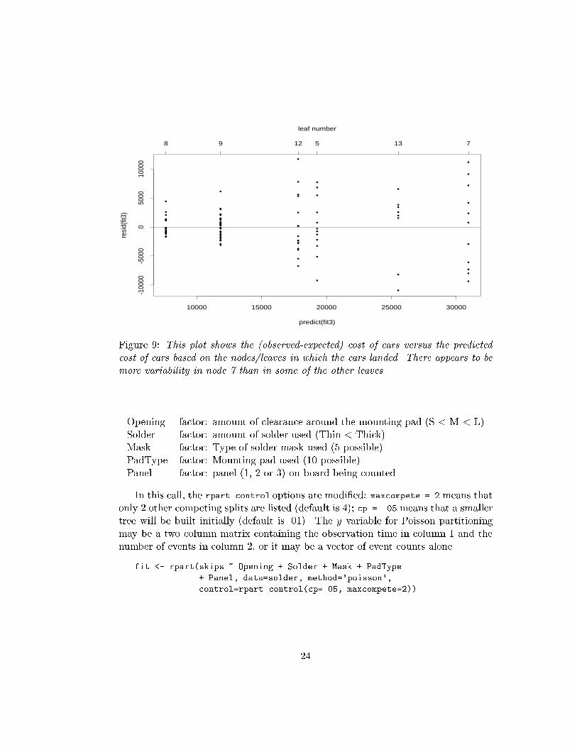
Finally, it is possible to look at the residuals from this model, just as with a

regular linear regression �t, as shown in the following �gure.

> plot(predict(fit3),resid(fit3))

> axis(3,at=fit3$frame$yval[fit3$frame$var=='<leaf>'],

labels=row.names(fit3$frame)[fit3$frame$var=='<leaf>'])

> mtext('leaf number',side=3, line=3)

> abline(h=0)

6.3 Solder data (poisson method)

The solder data frame, as explained in the Splus help �le, is a design object with 900

observations, which are the results of an experiment varying 5 factors relevant to the

wave-soldering procedure for mounting components on printed circuit boards. The

response variable, skips, is a count of how many solder skips appeared to a visual

inspection. The other variables are listed below:

23

•

•

•

•

•

••

•

•

•

••

•

•

•

•

•

•

•

•

•

•

•

•••

•

•

•

•

• •

•

•

••

•

•

••

• •

•

•

•

••

•

•

• •

•

•

•

••

•

•

•

••

•

•

•

•

•

••

•

•

•

•

•

••• •

•

•

•

•••

•

•

•

•

••

••••

•

••

• ••

•

•

•

•

•

•

predict(fit3)

resi

d(fit

3)

10000 15000 20000 25000 30000

-100

00-5

000

050

0010

000

8 9 12 5 13 7

leaf number

Figure 9: This plot shows the (observed-expected) cost of cars versus the predicted

cost of cars based on the nodes/leaves in which the cars landed. There appears to be

more variability in node 7 than in some of the other leaves.

Opening factor: amount of clearance around the mounting pad (S < M < L)

Solder factor: amount of solder used (Thin < Thick)

Mask factor: Type of solder mask used (5 possible)

PadType factor: Mounting pad used (10 possible)

Panel factor: panel (1, 2 or 3) on board being counted

In this call, the rpart.control options are modi�ed: maxcompete = 2 means that

only 2 other competing splits are listed (default is 4); cp = .05 means that a smaller

tree will be built initially (default is .01). The y variable for Poisson partitioning

may be a two column matrix containing the observation time in column 1 and the

number of events in column 2, or it may be a vector of event counts alone.

fit <- rpart(skips ~ Opening + Solder + Mask + PadType

+ Panel, data=solder, method='poisson',

control=rpart.control(cp=.05, maxcompete=2))

24

6.3.1 print function

The print command summarizes the tree, as in the previous examples.

n= 900



1) root 900 8788.0 5.530

2) Opening:M,L 600 2957.0 2.553

4) Mask:A1.5,A3,B3 420 874.4 1.033 *

5) Mask:A6,B6 180 953.1 6.099 *

3) Opening:S 300 3162.0 11.480

6) Mask:A1.5,A3 150 652.6 4.535 *

7) Mask:A6,B3,B6 150 1155.0 18.420 *

� The response value is the expected event rate (with a time variable), or in this

case the expected number of skips. The values are shrunk towards the global

estimate of 5.530 skips/observation.

� The deviance is the same as the null deviance (sometimes called the residual

deviance) that you'd get when calculating a Poisson glm model for the given

subset of data.

� The splitting rule is based on the likelihood ratio test for two Poisson groups

Dparent ��Dleft son +Dright son

�


> summary(fit,cp=.10)

Call:

rpart(formula = skips ~ Opening + Solder + Mask + PadType + Panel, data =

solder, method = "poisson", control = rpart.control(cp = 0.05,

maxcompete = 2))

n= 900


1 0.3038 0 1.0000 1.0051 0.05248

2 0.1541 1 0.6962 0.7016 0.03299

3 0.1285 2 0.5421 0.5469 0.02544

4 0.0500 3 0.4137 0.4187 0.01962

25


events=4977, estimated rate=5.53 , mean deviance=9.765


Primary splits:

Opening splits as RLL, improve=2670, (0 missing)

Mask splits as LLRLR, improve=2162, (0 missing)

Solder splits as RL, improve=1168, (0 missing)




Primary splits:

Mask splits as LLRLR, improve=1129.0, (0 missing)

Opening splits as RRL, improve= 250.8, (0 missing)

Solder splits as RL, improve= 219.8, (0 missing)




Primary splits:

Mask splits as LLRRR, improve=1354.0, (0 missing)

Solder splits as RL, improve= 976.9, (0 missing)

PadType splits as RRRRLRLRLL, improve= 313.2, (0 missing)

Surrogate splits:

Solder splits as RL, agree=0.6, adj=0.2, (0 split)









� The improvement is Devianceparent � (Devianceleft +Devianceright), which is

the likelihood ratio test for comparing two Poisson samples.

� The cross-validated error has been found to be overly pessimistic when de-

scribing how much the error is improved by each split. This is likely an e�ect

of the boundary e�ect mentioned earlier, but more research is needed.

26

|Opening:bc

Mask:abd Mask:ab

1.033433/420

6.0991098/180 4.535

680/15018.420

2766/150

|Opening:bc

Mask:ab 2.553

1531/600

4.535680/150

18.4202766/150

Figure 10: The �rst �gure shows the solder data, �t with the poisson method, using

a cp value of 0.05. The second �gure shows the same �t, but with a cp value of 0.15.

The function prune.rpart was used to produce the smaller tree.

� The variation xstd is not as useful, given the bias of xerror.

6.3.3 plot, text, prune functions

> plot(fit)

> text(fit,use.n=T)

> fit.prune <- prune(fit,cp=.15)

> plot(fit.prune)

> text(fit.prune,use.n=T)

The use.n=T option speci�es that number of events / total N should be listed

along with the predicted rate (number of events/person-years). The function prune

trims the tree fit to the cp value 0:15. The same tree could have been created by

specifying cp = .15 in the original call to rpart.

6.4 Stage C Prostate cancer (survival method)

One special case of the Poisson model is of particular interest for medical consulting

(such as the authors do). Assume that we have survival data, i.e., each subject has

27

either 0 or 1 event. Further, assume that the time values have been pre-scaled so as

to �t an exponential model. That is, stretch the time axis so that a Kaplan-Meier

plot of the data will be a straight line when plotted on the logarithmic scale. An

approximate way to do this is

temp <- coxph(Surv(time, status) ~1)

newtime <- predict(temp, type='expected')

and then do the analysis using the newtime variable. (This replaces each time value

by �(t), where � is the cumulative hazard function).

A slightly more sophisticated version of this which we will call exponential scaling

gives a straight line curve for log(survival) under a parametric exponential model.

The only di�erence from the approximate scaling above is that a subject who is

censored between observed death times will receive \credit" for the intervening in-

terval, i.e., we assume the baseline hazard to be linear between observed deaths. If

the data is pre-scaled in this way, then the Poisson model above is equivalent to

the local full likelihood tree model of LeBlanc and Crowley [3]. They show that this

model is more e�cient than the earlier suggestion of Therneau et. al. [6] to use the

martingale residuals from a Cox model as input to a regression tree (anova method).

Exponential scaling or method='exp' is the default if y is a Surv object.

Let us again return to the stage C cancer example. Besides the variables ex-

plained previously we will use pgtime, which is time to tumor progression.

> fit <- rpart(Surv(pgtime, pgstat) ~ age + eet + g2 + grade +

gleason + ploidy, data=stagec)

> print(fit)

n= 146



1) root 146 195.30 1.0000

2) grade<2.5 61 44.98 0.3617

4) g2<11.36 33 9.13 0.1220 *

5) g2>11.36 28 27.70 0.7341

10) gleason<5.5 20 14.30 0.5289 *

11) gleason>5.5 8 11.16 1.3140 *

3) grade>2.5 85 125.10 1.6230

6) age>56.5 75 104.00 1.4320

12) gleason<7.5 50 66.49 1.1490

24) g2<13.475 25 29.10 0.8817 *

25) g2>13.475 25 36.05 1.4080

28

50) g2>17.915 14 18.72 0.8795 *

51) g2<17.915 11 13.70 2.1830 *

13) gleason>7.5 25 34.13 2.0280

26) g2>15.29 10 11.81 1.2140 *

27) g2<15.29 15 19.36 2.7020 *

7) age<56.5 10 15.52 3.1980 *

> plot(fit, uniform=T, branch=.4, compress=T)

> text(fit, use.n=T)

Note that the primary split on grade is the same as when status was used as a

dichotomous endpoint, but that the splits thereafter di�er.

> summary(fit,cp=.02)

Call:

rpart(formula = Surv(pgtime, pgstat) ~ age + eet + g2 + grade + gleason +

ploidy, data = stagec)

n= 146


1 0.12913 0 1.0000 1.0060 0.07389

2 0.04169 1 0.8709 0.8839 0.07584

3 0.02880 2 0.8292 0.9271 0.08196

4 0.01720 3 0.8004 0.9348 0.08326

5 0.01518 4 0.7832 0.9647 0.08259

6 0.01271 5 0.7680 0.9648 0.08258

7 0.01000 8 0.7311 0.9632 0.08480


events=54, estimated rate=1 , mean deviance=1.338


Primary splits:

grade < 2.5 to the left, improve=25.270, (0 missing)

gleason < 5.5 to the left, improve=21.630, (3 missing)

ploidy splits as LRR, improve=14.020, (0 missing)

g2 < 13.2 to the left, improve=12.580, (7 missing)

age < 58.5 to the right, improve= 2.796, (0 missing)

Surrogate splits:


ploidy splits as LRR, agree=0.644, adj=0.148, (0 split)

g2 < 9.945 to the left, agree=0.630, adj=0.115, (0 split)


.

.

29

|grade<2.5

g2<11.36

gleason<5.5

age>56.5

gleason<7.5

g2<13.475

g2>17.915

g2>15.29

0.12201/33

0.52894/20

1.31404/8

0.88178/25

0.87955/14

2.18308/11

1.21405/10

2.702011/15

3.19808/10

Figure 11: The prostate cancer data as a survival tree

.

Suppose that we wish to simplify this tree, so that only four terminal nodes

remain. Looking at the table of complexity parameters, we see that prune(fit,

cp=.015) would give the desired result. It is also possible to trim the �gure interac-

tively using snip.rpart. Point the mouse on a node and click with the left button to

get some simple descriptives of the node. Double-clicking with the left button will

`remove' the sub-tree below, or one may click on another node. Multiple branches

may be snipped o� one by one; clicking with the right button will end interactive

mode and return the pruned tree.

> plot(fit)

> text(fit,use.n=T)

> fit2 <- snip.rpart(fit)

node number: 6 n= 75

response= 1.432013 ( 37 )

Error (dev) = 103.9783

> plot(fit2)

> text(fit2,use.n=T)

30

| | |grade<2.5

g2<11.36 age>56.5

0.12201/33

0.73418/28

1.432037/75

3.19808/10

Figure 12: An illustration of how snip.rpart works. The full tree is plotted in the

�rst panel. After selecting node 6 with the mouse (double clicking on left button),

the subtree disappears from the plot (shown in the second panel). Finally, the new

subtree is redrawn to use all available space and it is labelled.

31

05

10

15

0.0 0.2 0.4 0.6 0.8 1.0

Tim

e to

Pro

gre

ssio

n

Prob Progression

no

de

4n

od

e 5

no

de

6n

od

e 7

Figure

13:Survivalplotbased

on

snipped

rpart

objec

t.Theprobability

oftumor

progressio

nis

grea

test

innode7,whichhaspatie

nts

whoare

youngerandhavea

higherinitia

ltumorgrade.

Fora�nalsummary

ofthemodel,

itcanbehelp

fulto

plottheprobability

of

survivalbased

onthe�nalbinsinwhich

thesubjects

landed.Tocrea

tenew

varia

bles

based

ontherpartgroupings,use

where.Thenodes

offit2aboveare

show

nin

the

righthandpanelof�gure

12:node4has1event,33subjects,

grade=

1-2

andg2

<11.36;node5has8events,

28subjects,

grade=1-2

andg2>

11.36;node6has

37events,

75subjects,

grade=

3-4,age>

56.5;node7has8events,

10subjects,

grade=

3-4,age<

56.5.Patien

tswhoare

younger

andhaveahigher

initia

lgrade

tendto

havemore

rapid

progressio

nofdisea

se.

>newgrp<-fit2$where

>plot(survfit(Surv(pgtime,pgstat)~newgrp,data=stagec),

mark.time=F,lty=1:4)

>title(xlab='TimetoProgression',ylab='ProbProgression')

>legend(.2,.2,legend=paste('node',c(4,5,6,7)),lty=1:4)

References

[1]L.Breim

an,J.H.Fried

man,R.A.Olsh

en,,andC.J

Stone.

Classi�

catio

nand

Regressio

nTree

s.Wadsworth

,Belm

ont,Ca,1983.

32

[2] L.A. Clark and D. Pregibon. Tree-based models. In J.M. Chambers and T.J.

Hastie, editors, Statistical Models in S, chapter 9. Wadsworth and Brooks/Cole,

Paci�c Grove, Ca, 1992.

[3] M. LeBlanc and J Crowley. Relative risk trees for censored survival data. Bio-

metrics, 48:411{425, 1992.

[4] O. Nativ, Y. Raz, H.Z. Winkler, Y. Hosaka, E.T. Boyle, T.M. Therneau, G.M.

Farrow, R.P. Meyers, H. Zincke, and M.M Lieber. Prognostic value of ow

cytometric nuclear DNA analysis in stage C prostate carcinoma. Surgical Forum,

pages 685{687, 1988.

[5] T.M. Therneau and Atkinson E.J. An introduction to recursive partitioning

using the rpart routine. Technical Report 61, Mayo Clinic, Section of Statistics,

1997.

[6] T.M. Therneau, Grambsch P.M., and T.R. Fleming. Martingale based residuals

for survival models. Biometrika, 77:147{160, 1990.

33

al metho d) 27 - mayo

Documents