ALADDIN : A COMPUTATIONALTOOLKIT FOR INTERACTIVEENGINEERING MATRIX AND FINITEELEMENT ANALYSISMark Austin, Xiaoguang Chenand Wane-Jang LinInstitute for Systems ResearchandDepartment of Civil EngineeringUniversity of MarylandCollege Park, MD 20742November 17, 1995

AbstractThis report describes Version 1.0 of ALADDIN, an interactive computationaltoolkit for the matrix and �nite element analysis of engineering systems. The ALADDINpackage is designed around a language speci�cation, that includes quantities with physicalunits, branching constructs, and looping constructs. The basic language functionality isenhanced with external libraries of matrix and �nite element functions.ALADDIN's problem solving capabilities are demonstrated via the solution to aseries of matrix and numerical analysis problems. ALADDIN is employed in the �niteelement analysis of two building structures, and two highway bridge structures.

ContentsI INTRODUCTION TO ALADDIN 41 Introduction to ALADDIN 51.1 Problem Statement : : : : : : : : : : : : : : : : : : : : : : : : : : : : : : : 51.2 ALADDIN Components : : : : : : : : : : : : : : : : : : : : : : : : : : : : 71.3 Scope of this Report : : : : : : : : : : : : : : : : : : : : : : : : : : : : : : 11II MATRIX LIBRARY 122 Command Language for Quantity and Matrix Operations 132.1 How to Start (and Stop) ALADDIN : : : : : : : : : : : : : : : : : : : : : : 132.2 Format of General Command Language : : : : : : : : : : : : : : : : : : : : 142.3 Physical Quantities : : : : : : : : : : : : : : : : : : : : : : : : : : : : : : : 152.3.1 De�nition and Printing of Quantities : : : : : : : : : : : : : : : : : 152.3.2 Formatting of Quantity Output : : : : : : : : : : : : : : : : : : : : 172.3.3 Quantity Arithmetic : : : : : : : : : : : : : : : : : : : : : : : : : : 192.3.4 Making a Quantity Dimensionless : : : : : : : : : : : : : : : : : : : 212.3.5 Switching Units On and O� : : : : : : : : : : : : : : : : : : : : : : 212.3.6 Setting Units Type to US or SI : : : : : : : : : : : : : : : : : : : : 222.4 Control of Program Flow : : : : : : : : : : : : : : : : : : : : : : : : : : : : 242.4.1 Logical Operations : : : : : : : : : : : : : : : : : : : : : : : : : : : 242.4.2 Conditional Branching : : : : : : : : : : : : : : : : : : : : : : : : : 252.4.3 Looping and Stopping Commands : : : : : : : : : : : : : : : : : : : 262.5 De�nition and Printing of Matrices : : : : : : : : : : : : : : : : : : : : : : 292.5.1 De�nition of Small Matrices : : : : : : : : : : : : : : : : : : : : : : 292.5.2 Built-in Functions for Allocation of Matrices : : : : : : : : : : : : : 302.5.3 De�nition of Matrices with Units : : : : : : : : : : : : : : : : : : : 322.5.4 Printing Matrices with Desired Units : : : : : : : : : : : : : : : : : 342.6 Matrix-to-Quantity Conversion : : : : : : : : : : : : : : : : : : : : : : : : 362.7 Basic Matrix Operations : : : : : : : : : : : : : : : : : : : : : : : : : : : : 362.7.1 Retrieving the Dimensions of a Matrix : : : : : : : : : : : : : : : : 362.7.2 Matrix Copy and Matrix Transpose : : : : : : : : : : : : : : : : : : 372.7.3 Matrix Addition, Subtraction, and Multiplication : : : : : : : : : : 372.7.4 Scaling a Matrix by a Quantity : : : : : : : : : : : : : : : : : : : : 392.7.5 Euclidean Norm of Row/Column Vectors : : : : : : : : : : : : : : : 411

2.7.6 Minimum and Maximum Matrix Elements : : : : : : : : : : : : : : 422.7.7 Substitution/Extraction of Submatrices : : : : : : : : : : : : : : : : 432.8 Solution of Linear Matrix Equations : : : : : : : : : : : : : : : : : : : : : 452.8.1 Solving [A] fxg = fbg : : : : : : : : : : : : : : : : : : : : : : : : : : 462.8.2 Matrix Inverse : : : : : : : : : : : : : : : : : : : : : : : : : : : : : : 512.9 Matrix Eigenvalues and Eigenvectors : : : : : : : : : : : : : : : : : : : : : 552.9.1 Solving K� =M�� : : : : : : : : : : : : : : : : : : : : : : : : : : 56Numerical Example 1 : Buckling of Rod : : : : : : : : : : : : : : : 56Numerical Example 2 : Vibration of Cantilever Beam : : : : : : : : 613 Construction of Numerical Algorithms 683.1 Introduction : : : : : : : : : : : : : : : : : : : : : : : : : : : : : : : : : : : 683.2 Roots of Nonlinear Equations : : : : : : : : : : : : : : : : : : : : : : : : : 683.2.1 Newton-Raphson and Secant Algorithms : : : : : : : : : : : : : : : 683.2.2 Broyden-Fletcher-Goldfarb-Shanno (BFGS) Algorithm : : : : : : : 703.3 Han-Powell Algorithm for Optimization : : : : : : : : : : : : : : : : : : : : 773.3.1 Quadratic Programming (QP) : : : : : : : : : : : : : : : : : : : : : 773.3.2 Armijo Line Search Rule : : : : : : : : : : : : : : : : : : : : : : : : 783.3.3 The BFGS update and Han-Powell method : : : : : : : : : : : : : : 794 Computational Methods for Dynamic Analysis of Structures 884.1 Introduction : : : : : : : : : : : : : : : : : : : : : : : : : : : : : : : : : : : 884.2 Method of Newmark Integration : : : : : : : : : : : : : : : : : : : : : : : : 884.3 Method of Modal Analysis : : : : : : : : : : : : : : : : : : : : : : : : : : : 98III FINITE ELEMENT LIBRARY 1085 Finite Element Analysis Language 1095.1 Introduction : : : : : : : : : : : : : : : : : : : : : : : : : : : : : : : : : : : 1095.2 Structure of Finite Element Input Files : : : : : : : : : : : : : : : : : : : : 1095.3 Problem Speci�cation Parameters : : : : : : : : : : : : : : : : : : : : : : : 1115.4 Adding Nodes and Finite Elements : : : : : : : : : : : : : : : : : : : : : : 1115.5 Material and Section Properties : : : : : : : : : : : : : : : : : : : : : : : : 1135.6 Boundary Conditions : : : : : : : : : : : : : : : : : : : : : : : : : : : : : : 1165.7 External Nodal Loads : : : : : : : : : : : : : : : : : : : : : : : : : : : : : 1175.8 Sti�ness, Mass and External Loading Matrices : : : : : : : : : : : : : : : : 1175.9 Internal Loads : : : : : : : : : : : : : : : : : : : : : : : : : : : : : : : : : : 1185.10 Retrieving Information from ALADDIN : : : : : : : : : : : : : : : : : : : 1195.11 Library of Finite Elements : : : : : : : : : : : : : : : : : : : : : : : : : : : 1216 Input Files for Finite Element Analysis Problems 1286.1 Linear Static Analyses : : : : : : : : : : : : : : : : : : : : : : : : : : : : : 1286.1.1 Analysis of Five Story Moment Resistant Frame : : : : : : : : : : : 1286.1.2 Working Stress Design (WSD) of Simpli�ed Bridge : : : : : : : : : 1412

6.1.3 Three-Dimensional Analysis of Highway Bridge : : : : : : : : : : : 1566.2 Time-History Analyses : : : : : : : : : : : : : : : : : : : : : : : : : : : : : 1726.2.1 Modal Analysis of Five Story Steel Frame : : : : : : : : : : : : : : 172IV ARCHITECTURE AND DESIGN 1867 Data Types : Physical Quantity and Matrix Data Structures 1877.1 Introduction : : : : : : : : : : : : : : : : : : : : : : : : : : : : : : : : : : : 1877.2 Physical Quantities : : : : : : : : : : : : : : : : : : : : : : : : : : : : : : : 1877.2.1 Relationship between Quantity and Units : : : : : : : : : : : : : : : 1887.2.2 US and SI Units Conversion : : : : : : : : : : : : : : : : : : : : : : 1897.3 Matrices : : : : : : : : : : : : : : : : : : : : : : : : : : : : : : : : : : : : : 1917.3.1 Skyline Matrix Storage : : : : : : : : : : : : : : : : : : : : : : : : : 1937.3.2 Units Bu�ers for Matrix Multiplication : : : : : : : : : : : : : : : : 1967.3.3 Units Bu�ers for Inverse Matrix : : : : : : : : : : : : : : : : : : : : 1968 Architecture and Design of ALADDIN 2018.1 Introduction : : : : : : : : : : : : : : : : : : : : : : : : : : : : : : : : : : : 2018.2 Program Modules and Key Data Structures : : : : : : : : : : : : : : : : : 2018.3 Design and Implementation of Stack Machine : : : : : : : : : : : : : : : : 2088.3.1 Example of Machine Stack Execution : : : : : : : : : : : : : : : : : 2118.4 Language Design and Implementation : : : : : : : : : : : : : : : : : : : : : 217V CONCLUSIONS AND FUTURE WORK 2289 Conclusions and Future Work 2299.1 Conclusions : : : : : : : : : : : : : : : : : : : : : : : : : : : : : : : : : : : 2299.2 Future Work : : : : : : : : : : : : : : : : : : : : : : : : : : : : : : : : : : : 230

3

Part IINTRODUCTION TO ALADDIN

4

Chapter 1Introduction to ALADDIN1.1 Problem StatementThis report describes the development and capabilities of ALADDIN (Version1.0), an interactive computational toolkit for the matrix and �nite element analysisof engineering systems. The current target application area for ALADDIN is designand analysis of traditional Civil Engineering structures, such as highway bridges andearthquake-resistant buildings. With literally hundreds of engineering analysis and opti-mization computer programs having been written in the past 10-20 years (see references[1, 6, 23, 24, 26, 25, 29, 30] for some examples), a reader might rightfully ask who needsto write another engineering analysis package ?We respond to this challenge, and motivate the short- and long-term goals of thiswork by �rst noting that during the past two decades, computers have been providingapproximately 25% more power per dollar per year. Advances in computer hardware andsoftware have allowed for the exploration of many new ideas, and have been a key catalystin what has led to the maturing of computing as a discipline. In the 1970's computerswere viewed primarly as machines for research engineers and scientists { compared to to-day's standards, computer memory was very expensive, and central processing units wereslow. Early versions of structural analysis and �nite element computer programs, suchas ABAQUS [1], ANSR [23], and FEAP [30] were written in the FORTRAN computerlanguage, and were developed with the goal of optimizing numerical and/or instructionalconsiderations alone. These programs o�ered a restricted, but well implemented, setof numerical procedures for static structural analyses, and linear/nonlinear time-historyresponse calculations. And even though these early computer programs were not partic-ularly easy to use, practising engineers gradually adopted them because they allowed forthe analysis of new structural systems in a ways that were previously intractable.During the past twenty years, the use of computers in engineering has matured tothe point where importance is now placed on ease of use, and a wide-array of services be-ing made available to the engineering profession as a whole. Computer programs writtenfor engineering computations are expected to be fast and accurate, exible, reliable, and5

of course, easy to use. Whereas an engineer in the 1970's might have been satis�ed by acomputer program that provided numerical solutions to a very speci�c engineering prob-lem, the same engineer today might require the engineering analysis, plus computationalsupport for design code checking, optimization, interactive computer graphics, networkconnectivity, and so forth. Many of the latter features are not a bottleneck for gettingthe job done. Rather, features such as interactive computer graphics simply make the jobof describing a problem and interpreting results easier { the pathway from ease-of-use toproductivity gains is well de�ned. It is also well worth noting that computers once viewedas a tool for computation alone, are now seen as an indispensable tool for computationand communications. In fact, the merging of computation and communications is mak-ing fundamental changes to the way an engineer conducts his/her day-to-day businessactivities. Consider, for example, an engineer who has access to a high speed personalcomputer with multimedia interfaces and global network connectivity, and who happensto be part of a geographically dispersed development team. The team members can usethe Internet/E-mail for day-to-day communications, to conduct engineering analyses atremote sites, and to share design/analysis results among the team members. Clear com-munication of engineering information among the team members may be of paramountimportance in determining the smooth development of a project.The di�culty in following-up on the abovementioned hardware advances withappropriate software developments is clearly re ected in the economic costs of projectdevelopment. In the early 1970's software consumed approximately 25% of total costs,and hardware 75% of total costs for development of data intensive systems. Nowadays,development and maintenance of software typically consumes more than 80% of the totalproject costs. This change in economics is the combined result of falling hardware costs,and increased software development budgets needed to implement systems that are muchmore complex than they used to be. Whereas one or two programmers might have writ-ten a complete program twenty years ago, today's problems are so complex that teamsof programmers are needed to understand a problem and �ll-in the details of requireddevelopment.When a computer program has a poorly designed architecture, its integrationwith another package can be very di�cult, with the result often falling short of users'expectations. Let's suppose, for example, that we wanted to interface the �nite elementpackage FEAP [30] with the interactive optimization-based design environment calledDELIGHT [6, 24, 29]. Since FEAP was not written with interfaces to external envi-ronments as a design criterion, a programmer(s) faced with this task would �rst need to�gure out how FEAP and DELIGHT work (not an easy task), and then devise a map-ping from DELIGHT's external interface routines to FEAP's subroutines. In the �rstwriter's opinion, such a mapping is likely to exist, but only after several subroutines havebeen added to FEAP. The programmer(s) would need the computer skills and tenacityto stick-with the lengthy period of code development that would ensue. And what aboutthe result ? In our experience [3, 4, 6], the integrated DELIGHT-FEAP tool would mostlikely do a very good job of solving a narrow range of problems, and as such, have ashort life cycle. These barriers to integration are frustrating because �nite element and6

optimization procedures are essentially specialized matrix computations { the disciplinesshould �t together in almost a seamless way. In our opinion, the main barrier to softwareintegration is an ad-hoc approach to software tool development in the �rst place.Rather than simply repeat the \scenario procedure" for yet another set of pack-ages, this research project attempts to understand the structure matrix, �nite element,and optimization packages should take so that they can be integrated in a natural way.Project ALADDIN begins with the design and implementation of a system speci�cationthat includes:[1] A Model : The model will include data structures for the information to be stored,and a stack machine for the execution of the matrix and �nite element algorithms.[2] A Language : The language will be a means for describing the matrices and �niteelement mesh { it will act as the user interface to the underlying model.In traditional approaches to problem solving, engineers write the details of a problemand its solution procedure on paper. They use physical units to add clarity to theproblem description, and may specify step-by-step details for a numerical solutionto the problem. We would like the ALADDIN language to be textually descriptive,and strike a balance between simplicity and extensibility. It should use a smallnumber of data types and control structures, incorporate physical units, and yet, bedescriptive enough so that the pencil and paper and ALADDIN problem description�les are almost the same.[3] Defined Steps and Ordering of the Steps : The steps will de�ne the transfor-mations (e.g. nearly all engineering processes will require iteration and branching)that can be carried out on system components.[4] Guidance for Applying the Specification : Guidance includes factors such asdescriptive problem description �les and documentation.Our research direction is inspired in part by the systems integration methods developedfor the European ESPRIT Project [20], and by the success of C. Although the C program-ming language has only 32 keywords, and a handful of control structures, its judiciouscombination with external libraries has resulted in the language being used in a very widerange of applications.1.2 ALADDIN ComponentsFigure 1.1 is a schematic of the ALADDIN (Version 1.0) architecture, and showsits three main parts: (1) the kernel; (2) libraries of matrix and �nite element functions,and (3) the input �le(s).Speci�c engineering problems are de�ned in ALADDIN problem description �les,and solved using components of ALADDIN that are part interpreter-based, and part7

INPUT FILE

Block of Input Statements

Block of Input Statements

Block of Input Statements

FINITE ELEMENT LIBRARY

MATRIX LIBRARY

LIBRARIES OF BUILTIN C FUNCTIONS

ALADDIN KERNEL AND INPUT FILES

ALADDIN’S KERNEL

[ STACK MACHINE ]

Figure 1.1: High Level Components in ALADDIN (Version 1.0)compiled C code. It is important to keep in mind that as the speed of CPU processorsincreases, the time needed to prepare a problem description increases relative to thetotal time needed to work through an engineering analysis. Hence, clarity of an input�le's contents is of paramount importance. In the design of the ALADDIN language weattempt to achieve these goals with: (1) liberal use of comment statements (as with theC programming language, comments are inserted between /* .... */), (2) consistentuse of function names and function arguments, (3) use of physical units in the problemdescription, and (4) consistent use of variables, matrices, and structures to control the ow of program logic.ALADDIN problem descriptions and their solution algorithms are a compositionof three elements: (1) data, (2) control, and (3) functions [27]:[1] Data : ALADDIN supports three data types, \character string" for variable names,physical quantities, and matrices of physical quantities for engineering data. For example,the script of codexCoord = 2 m;xVelociy = 2 m / sec;de�nes two physical quantities, xCoord as 2 meters, and xVelocity as 2 meters persecond. Floating point numbers are stored with double precision accuracy, and are viewedas physical quantities without units. There are no integer data types in ALADDIN.[2] Control : Control is the basic mechanisms in a programming language for the spec-i�cation of looping constructs and conditional branching.8

ENTRY EXIT ENTRY

S2

S1

EXPR

TRUE

FALSE

TRUE

EXPRS1EXITFALSE

BRANCHING CONSTRUCTS LOOPING CONSTRUCTSFigure 1.2: Branching and Looping Constructs in ALADDINIn Chapter 2 we will see that ALADDIN supports the while and for looping constructs,and the if and if-then-else branching constructs. The data and control componentsof the ALADDIN language are implemented as a �nite-state stack machine model, whichfollows in the spirit of work presented by Kernighan and Pike [18]. ALADDIN's stackmachine reads blocks of command statements from either a problem description �le, or thekeyboard, and converts them into an array of machine instructions. The stack machinethen executes the statements.[3] Functions : The functional components of ALADDIN provide hierarchy to the so-lution of our matrix and �nite element processes, and are located in libraries of compiledC code, as shown on the right-hand side of Figure 1.1. Version 1.0 of ALADDIN hasfunctional support for basic matrix operations, that includes numerical solutions to linearequations, and the symmetric eigenvalue problem. A library of �nite element functions isprovided.FUNCTION OutputInput

RETURN TYPE = FUNCTION NAME ( Arg 1 , Arg 2 , ........ , Arg N );

InputOutputFigure 1.3: Schematic of Functions in ALADDINFigure 1.3 shows the general components of a function call, it's input argument list, andthe function return type. A key objective in the language design is to devise families oflibrary functions that will make ALADDIN's problem solving ability as wide as possible.Version 1.0 of ALADDIN does not support user-de�ned functions in the input-�le9

(or keyboard) command language.The strategy we have followed in ALADDIN's development is to keep the numberand type of arguments employed in library function calls small. Whenever possible, thefunction's return type and arguments should be of the same data type, thereby allowingthe output from one or more functions to act as the input to following function call. Moreprecisely, we would like to write input code that takes the formreturntype1 = Function1(); /* <= application area 1 */returntype2 = Function2(); /* <= application area 1 */returntype3 = Function3( returntype1, returntype2 ); /* <= application area 2 */or evenreturntype3 = Function3( Function1(), Function2() );If Function1() and Function2() belong to application area 1 (e.g. matrix analysis), andFunction3() belongs to application area 2 (e.g. �nite element analysis; optimization),then this language structure allows application areas 1 and 2 to be combined in a naturalway. In Chapters 2 to 6, we will see that most of the built-in functions accept one or twomatrix arguments, and return one matrix argument. Occasionally, we will see built-infunction that have more than two function arguments, and return a quantity instead ofa matrix. Collections of quantities are returned from functions by bundling them into asingle matrix { the individual quantities are then extracted as elements of the functionreturn type. Factor Interpreted Code Compiled CodeUser Control High Very LowRequired User Knowledge High MediumSpeed of Execution Slow FastTable 1.1: Trade-O�s { Interpreted Code Versus Compiled CodeTable 1.1 contains a summary of trade-o�s between the use of interpreted code versuscompiled C code. A key advantage of interpreters is exibility { problem parametersand algorithms may be modi�ed during the problem solving process, and without havingto recompile source code. This feature reduces the time needed to work through aninteration of the problem solving process. The well known trade-o� is speed of execution.Interpreted code executes much slower { approximately ten times slower { than compiledC code. Consequently, we expect that as ALADDIN evolves, new algorithms will bedeveloped in tested as interpreted code, and once working, will be converted into librariesof compiled C code having an interface that �ts-in with the remaining library functions.10

1.3 Scope of this ReportThis report is divided into four parts. In Part II we will see that the ALADDINlanguage supports variable arithmetic with physical units, matrix operations with units,and looping and branching control structures, where decisions are made with quantitieshaving physical units. Chapters 3 and 4 demonstrate use of the ALADDIN language viaa suite of problems { we compute the roots of nonlinear equations, demonstrate the Han-Powell method of optimization, and solve several problems from structural engineeringand structural dynamics.Part III of this report describes the built-in functions for the generation of �nite el-ement meshes, external loads, and �nite element modeling assumptions. We demonstratethese features by solving a variety two- and three-dimensional �nite element problems.We have written Part IV for ALADDIN developers, who may need to understandthe data structures and algorithms used to read and store matrices, to create and store�nite element meshes, and to construct the stack machine. Readers of this section areassumed to have a good working knowledge of the C programming language.

11

Part IIMATRIX LIBRARY

12

Chapter 2Command Language for Quantityand Matrix OperationsThe purposes of this chapter are to explain execution of the ALADDIN envi-ronment, and details of the matrix command language within ALADDIN. For ease ofreading, and when space permits, output from ALADDIN is juxtaposed with the inputcommand(s).2.1 How to Start (and Stop) ALADDINALADDIN's command line arguments are setup in a very exible way. The �rstargument is simply ALADDIN, the name of the executable program.Input from KeyboardALADDIN -[ks]Input from a FileALADDIN -[sf] <filename>Command options have the following meaning:-f Indicate input from a �le (it must be accompanied by a �lename).-k Indicates input from the keyboard. When input is generated via the keyboard, ainput history �le will be generated and named as input�le.std. In the likely eventof mistyping or a syntax error, you can continue type in input�le.std.-s All input will be scanned for syntax errors without actually executing the program.13

The command ALADDIN must be accompanied by either the -f ag, or the -k ag. The-s ag is optional. Command line options can be typed in arbitrary sequences.The command to exit from ALADDIN isquit;Don't forget the semicolon.2.2 Format of General Command LanguageThe ALADDIN command language corresponds to individual statements, andsequences of statements.statement 1;statement 2;........statement N;Each statement ends with a semi-colon (;). Comment statements (as with the C pro-gramming language, comments are enclosed between /* .... */), as in/** ================================* Here is a block of N statements.* ================================*/statement 1; /* the first ALADDIN statement */statement 2; /* the second ALADDIN statement */........statement N; /* the n^th ALADDIN statement */Basic output of character strings and physical quantities is handled with the print com-mand. For example,print "Here is one line of output \n";gives Here is one line of outputCharacter strings are enclosed within quotes (i.e "....."). The escape character (nn)forces output onto a new line. 14

2.3 Physical QuantitiesWhile the importance of the engineering units is well known [11, 13, 17], physicalunits are not a standard part of many main-stream �nite element software packages {indeed, most engineering software packages simply hold the engineer responsible for mak-ing sure engineering units are consistent, While this practice of implementation may besatisfactory for computation of well established algorithms, it is almost certain to leadto incorrect results when engineers are working on the development of new and innova-tive computations. ALADDIN deviates from this trend by providing support for basicarithmetic operations on quantities and matrices of physical quantities.2.3.1 De�nition and Printing of QuantitiesLet's begin with the basics. A quantity is a number with physical units. To assignthe quantity \2 m" to variable \x" just typex = 2 m;The semi-colon character \;" is required for every command to indicate the end of theone statement. The following script of code demonstrates de�nition of quantities.INPUT OUTPUTprint " LENGTH UNITS : SI SYSTEM \n"; LENGTH UNITS : SI SYSTEMx = 1 mm; y = 1 cm; z = 1 dm;u = 1 m; v = 1 km;print "x = ", x, "\n"; x = 1 mmprint "y = ", y, "\n"; y = 1 cmprint "z = ", z, "\n"; z = 1 dmprint "u = ", u, "\n"; u = 1 mprint "v = ", v, "\n"; v = 1 kmprint "\n VOLUME UNITS : US \n"; VOLUME UNITS : USx = 1 gallon; y = 1 barrel;print "x = ", x, "\n"; x = 1 gallonprint "y = ", y, "\n"; y = 1 barrelprint "\n MASS UNITS : SI SYSTEM \n"; MASS UNITS : SI SYSTEMx = 1 g; y = 1 kg; z = 1 Mg;print "x = ", x, "\n"; x = 1 gprint "y = ", y, "\n"; y = 1 kgprint "z = ", z, "\n"; z = 1 Mg15

print " TIME UNITS : SI SYSTEM \n"; TIME UNITS : SI SYSTEMx = 1 sec; y = 1 ms;z = 1 min; u = 1 hr;print "x = ", x, "\n"; x = 1 secprint "y = ", y, "\n"; y = 1 msprint "z = ", z, "\n"; z = 1 minprint "u = ", u, "\n"; u = 1 hrprint "\n TEMPERATURE UNITS : SI SYSTEM \n"; TEMPERATURE UNITS : SI SYSTEMx = 1 deg_C;print "x = ", x, "\n"; x = 1 deg_Cprint "\n TEMPERATURE UNITS : US SYSTEM \n"; TEMPERATURE UNITS : US SYSTEMx = 1 deg_F;print "x = ", x, "\n"; x = 1 deg_Fprint "\n UNITS OF FREQUENCY & SPEED \n"; UNITS OF FREQUENCY & SPEEDx = 1 Hz;y = 1 rpm; /* rev. per min */z = 1 cps; /* cycle per sec */print "x = ", x, "\n"; x = 1 Hzprint "y = ", y, "\n"; y = 1 rpmprint "z = ", z, "\n"; z = 1 cpsprint "\n FORCE UNITS : SI SYSTEM \n"; FORCE UNITS : SI SYSTEMx = 1 N; y = 1 kN; z = 1 kgf;print "x = ", x, "\n"; x = 1 Nprint "y = ", y, "\n"; y = 1 kNprint "z = ", z, "\n"; z = 1 kgfprint "\n PRESSURE UNITS : SI SYSTEM \n"; PRESSURE UNITS : SI SYSTEMx = 1 Pa; y = 1 kPa;z = 1 MPa; u = 1 GPa;print "x = ", x, "\n"; x = 1 Paprint "y = ", y, "\n"; y = 1 kPaprint "z = ", z, "\n"; z = 1 MPaprint "u = ", u, "\n"; u = 1 GPaprint "\n ENERGY UNITS : SI SYSTEM \n"; ENERGY UNITS : SI SYSTEMx = 1 Jou; y = 1 kJ;print "x = ", x, "\n"; x = 1 Jouprint "y = ", y, "\n"; y = 1 kJ16

print "\n POWER UNITS : SI \n"; POWER UNITS : SIx = 1 Watt; y = 1 kW;print "x = ", x, "\n"; x = 1 Wattprint "y = ", y, "\n"; y = 1 kWprint "\n UNITS OF PLANE ANGLE UNITS \n"; UNITS OF PLANE ANGLE UNITSx = 1 deg; y = 1 rad;print "x = ", x, "\n"; x = 1 degprint "y = ", y, "\n"; y = 1 radThese examples focus on the SI system of units. In the US system, units of length areprovided for micro inches (micro in), inches (in), feet (ft), yards (yard), and miles(mile). Similarly, US units of mass are provided for pounds (lb), grains (grain), kilopounds (klb), and tons (ton). Units of force in the US system are pounds force (lbf)and one thousand pounds force (kips). Corresponding units of pressure in the US systemare pounds per square inch (psi), and thousands of pounds per square inch (ksi).Restrictions on Quantity Names : Like many other programming languages, theALADDIN command language has keywords and constants which are reserved for specialpurposes { they cannot be used for arbitrary purposes, such as variable names. Forexample, ALADDIN reserves the characters \N" and \m" for engineering units Newtonand metre. Similar restrictions apply to all units, keywords de�ning looping and controlconstructs (e.g. for and while), as well as built-in function names.A complete list of keywords and constants is given in Table 2.1. Table 2.2contains a list of names that are reserved for mathematical functions. Reserved namesfor matrix allocation functions, and functions to compute matrix operations, are given inTables 2.3 and 2.4, respectively. Reserved names also apply to names of functions forsolving linear equations, eigenvalues and eigenvectors, as well as �nite element analysis.These names are listed in Tables 2.5, 2.6, 5.1, 5.2, and in the text of Chapter 5.2.3.2 Formatting of Quantity OutputThe command option "(< units >)" allows for the printing of a quantity witha desired units. The following script of code gives some examples:INPUT OUTPUTprint " LENGTH UNITS \n"; LENGTH UNITSv = 1 km; w = 1 mile; 17

print "v = ", v , "\n"; v = 1 kmprint "v = ", v (in) , "\n"; v = 3.937e+04 inprint "v = ", v (ft) , "\n"; v = 3281 ftprint "v = ", v (yard), "\n"; v = 1094 yardprint "v = ", v (mile), "\n"; v = 0.6214 mileprint "w = ", w , "\n"; w = 1 mileprint "w = ", w (mm) , "\n"; w = 1.609e+06 mmprint "w = ", w (cm) , "\n"; w = 1.609e+05 cmprint "w = ", w (dm) , "\n"; w = 1.609e+04 dmprint "w = ", w (m ) , "\n"; w = 1609 mprint "w = ", w (km) , "\n"; w = 1.609 kmprint "\n VOLUME UNITS \n"; VOLUME UNITSx = 1 gallon;print "x = ", x , "\n"; x = 1 gallonprint "x = ", x (m^3), "\n"; x = 0.003785 m^ 3.0print "x = ", x (ft^3), "\n"; x = 0.1337 ft^ 3.0print "x = ", x (cm^3), "\n"; x = 3785 cm^ 3.0print "x = ", x (in^3), "\n"; x = 231 in^ 3.0print "x = ", x (barrel), "\n"; x = 0.02381 barrelprint "\n TEMPERATURE UNITS \n";i TEMPERATURE UNITSx = 1 deg_C; U = 10 mm/DEG_C;y = 1 deg_F; V = 10 in/DEG_F;print "x = ", x , "\n"; x = 1 deg_Cprint "x = ", x (deg_F), "\n"; x = 33.8 deg_Fprint "y = ", y , "\n"; y = 1 deg_Fprint "y = ", y (deg_C), "\n"; y = -17.22 deg_Cprint "U = ", U, "\n"; U = 10 mm/DEG_Cprint "V = ", V, "\n"; V = 10 in/DEG_Fprint "\n";print "U*(1 DEG_C) = ", U*(1 DEG_C) (mm), "\n"; U*(1 DEG_C) = 10 mmprint "U*(1 DEG_F) = ", U*(1 DEG_F) (mm), "\n"; U*(1 DEG_F) = 5.556 mmprint "V*(1 DEG_C) = ", V*(1 DEG_C) (in), "\n"; V*(1 DEG_C) = 18 inprint "V*(1 DEG_F) = ", V*(1 DEG_F) (in), "\n"; V*(1 DEG_F) = 10 inprint " TIME UNITS \n"; TIME UNITSx = 1 hr;print "x = ", x, "\n"; x = 1 hrprint "x = ", x (min), "\n"; x = 60 minprint "x = ", x (sec), "\n"; x = 3600 secprint "\n UNITS OF FREQUENCY & SPEED \n"; UNITS OF FREQUENCY & SPEEDy = 60 rpm; /* rev. per min */print "y = ", y, "\n"; y = 60 rpm18

print "y = ", y (Hz), "\n"; y = 1 Hzprint "y = ", y (cps), "\n"; y = 1 cpsprint "\n PLANE ANGLE UNITS \n"; PLANE ANGLE UNITSx = 180 deg; y = PI;print "x = ", x, "\n"; x = 180 degprint "x = ", x (rad), "\n"; x = 3.142 radprint "y = ", y, "\n"; y = 3.1416e+00print "y = ", y (deg), "\n"; y = 180 degSimilar conversion factors exist for units of mass, force, pressure, energy and power.2.3.3 Quantity ArithmeticPhysical units may be manipulated with basic multiply, division and power oper-ations. The following script of code demonstrates the range of arithmetic operations thatare possible: INPUT OUTPUTx = 10 g; y = 1 kg; z = 1 m;print "\nADDITION & SUBTRACTION \n"; ADDITION & SUBTRACTIONprint "x + y = ", x + y, "\n"; x + y = 1.01 kgprint "x - y = ", x - y, "\n"; x - y = -0.99 kgprint "\n MULTIPLY \n"; MULTIPLYprint "x * y = ", x * y, "\n"; x * y = 10 g.kgprint "x * z = ", x * z, "\n"; x * z = 10 g.mprint "\n DIVISION \n"; DIVISIONprint "x / y = ", x / y, "\n"; x / y = 1.0000e-02print "x / z = ", x / z, "\n"; x / z = 10 g/mprint "1 / z = ", 1 / z, "\n"; 1 / z = 1 m^-1.0print "z / 2 = ", z / 2 ,"\n"; z / 2 = 0.5 mprint "1/(x*y) = ", 1/(x*y),"\n"; 1/(x*y) = 0.1 1/(g.kg)print "z/(x*y) = ", z/(x*y),"\n"; z/(x*y) = 0.1 m/g.kgprint "(x*y)/z = ", (x*y)/z,"\n"; (x*y)/z = 10 g.kg/mprint "\n MATH CALCULATIONS \n"; MATH CALCULATIONSu = 30 deg;v = -PI/2;w = 2;print "sin(u) = ", sin(u), "\n"; sin(u) = 5.0000e-01print "sin(v) = ", sin(v), "\n"; sin(v) = -1.0000e+00print "cos(u) = ", cos(u), "\n"; cos(u) = 8.6603e-01print "cos(v) = ", cos(v), "\n"; cos(v) = 6.1230e-1719

print "tan(PI/4) = ", tan(PI/4), "\n"; tan(PI/4) = 1.0000e+00print "atan(1) = ", atan(1), "\n"; atan(1) = 7.8540e-01print "abs(-3 m) = ", abs(-3 m), "\n"; abs(-3 m) = 3 mprint "abs(v) = ", abs(v), "\n"; abs(v) = 1.5708e+00print "log(1E+5) = ", log(1E+5), "\n"; log(1E+5) = 1.1513e+01print "log10(1E+5)= ", log10(1E+5),"\n"; log10(1E+5)= 5.0000e+00print "exp(w) = ", exp(w), "\n"; exp(w) = 7.3891e+00We use the print command and the character string "nn" containing the newline toprint physical quantities and statements. Characters inside the equation marks \ " areconsidered statements. Arguments to mathematical functions, such as log() and exp()take dimensionless quantities. Trigonometric functions can, however, take arguments withthe units degree and radian because the latter are non-dimensional.Power operations on quantities do not work in quite the same way as the basicadd, subtract, multiply and divide operations on quantities. If quantity1 and quantity2are physical quantities, then the operationquantity1 ^ quantity2;is de�ned for dimensionless quantity1 and quantity2, and cases where one of the twooperands, but not both operands, has units. Unlike the basic arithmetic operations,which are evaluated left-to-right, expressions involving power operations are evaluatedfrom right-to-left. Here are some examples:INPUT OUTPUTprint "\n POWER \n"; POWERprint "2^2^3 = ", 2^2^3 , "\n"; 2^2^3 = 256print "(2 m)^2 = ", (2 m)^2 , "\n"; (2 m)^2 = 4 m^2print "2^2 m = ", 2^2 m , "\n"; 2^2 m = 4 mprint "2^2^2 m = ", 2^2^2 m , "\n"; 2^2^2 m = 16 mprint "10^4 N/m = ", 10^4 N/m , "\n"; 10^4 N/m = 1e+04 N/mprint "10^2^2 N/m = ", 10^2^2 N/m , "\n"; 10^2^2 N/m = 1e+04 N/mprint "0.25*2^2 m = ", 0.25*2^2 m, "\n"; 0.25*2^2 m = 1 mprint "1/2*2 m = ", 1/2*2 m, "\n"; 1/2*2 m = 1 mprint "(1/2*2 m) = ", (1/2*2 m), "\n"; (1/2*2 m) = 1 mprint "(1/2^2 m) = ", (1/2^2 m), "\n"; (1/2^2 m) = 0.25 1/mprint "(1/2^2)*(1 m) = ", (1/2^2)*(1 m), "\n"; (1/2^2)*(1 m) = 0.25 mprint "1/2^2*(1 m) = ", 1/2^2 *(1 m), "\n"; 1/2^2*(1 m) = 0.25 mx = 100 kg; z = 10 m;print "sqrt(100 kg) = ", sqrt(x) , "\n"; sqrt(100 kg) = 10 kg^0.5print "z^2 = ", z^2 , "\n"; z^2 = 100 m^2print "z^-3 = ", z^-3, "\n"; z^-3 = 0.001 1/m^3print "(x*z)^1 = ", (x*z)^1, "\n"; (x*z)^1 = 1000 m.kgprint "(x*z)^2 = ", (x*z)^2, "\n"; (x*z)^2 = 1e+06 m^2.kg^220

As mentioned above, power operations such asx = (1 m)^(2 sec);are illegal, and will cause ALADDIN to terminate its execution.An important feature of quantity operations is the check for consistent units.Suppose, for example, we try to add a quantity with time units to a second quantityhaving units of length, ALADDIN provides an appropriate fatal error messagex = 1 in; y = 1 sec;z = x + y;FATAL ERROR >> In Add() : Inconsistent Dimensions.FATAL ERROR >> Compilation Aborted.followed by the termination of program execution.2.3.4 Making a Quantity DimensionlessIn the development of algorithms to solve engineering problems, we will sometimesneed to strip (or remove) the units from a physical quantity, and work with the numer-ical value alone. The built-in function QDimenLess() removes units from quantities, asdemonstrated in the following script of code:INPUT OUTPUTprint "\n MAKE A QUANTITY DIMENSIONLESS \n"; MAKE A QUANTITY DIMENSIONLESSx = 1 N; y = 1 cm/sec;z = QDimenLess(x); u = QDimenLess(y);print "x (with dimen) = ", x, "\n"; x (with dimen) = 1 Nprint "y (with dimen) = ", y, "\n"; y (with dimen) = 0.01 m/secprint "x (without dimen) = ", z, "\n"; x (without dimen) = 1.0000e+00print "y (without dimen) = ", u, "\n"; y (without dimen) = 1.0000e-022.3.5 Setting Units Type to US or SIThe default units type is SI. The function SetUnitsType("string"), where"string" equals "SI" or "US", sets the units to SI or US, respectively.You should call SetUnitsType() before the �nite element displacements andstresses are printed (i.e. using PrintDispl() and PrintStress()).21

2.3.6 Switching Units On and O�The command SetUnitsOn turns the checking of units on, and the commandSetUnitsOff turns the checking of units o�. The default units option is SetUnitsOn.

22

Category List of Reserved NamesConstants DEG = 57.29577951308, E = 2.718281828459, GAMMA= 0.577215664901, and PI = 3.141592653589Keywords break, else, for, if, print, quit, read, return, SetUnitsOn,SetUnitsO�, then, whileSI Units micron, mm, cm, dm, m, km, g, kg, mg, N, kN, kgf, Pa,kPa, MPa, GPa, deg C, DEG C, Jou, kJ, Watt, kW, Hz,rpm, cpsUS Units in, ft, yard, mile, mil, micro in, lb, klb, ton, grain, lbf,kips, psi, ksi, deg F, DEG F, gallon, barrel, sec, ms, min,hr, deg, radTable 2.1: List of ALADDIN Keywords and ConstantsName/Argument Purpose of Functioncos(x) Compute cosine of quantity x. Default units are radianssin(x) Compute sin of quantity x. Default units are radianstan(x) Compute tangent of quantity x. Default units are radiansabs(x) Return absolute value of quantity x.exp(x) Compute exponential of quantity x.integer(x) Return integer component of quantity x.log(x) Compute natural logarithm of quantity x.log10(x) Compute logarithm, base 10, of quantity x.pow(x,n) Compute quantity x raised to the power n; n is a number.sqrt(x) Compute square root of quantity x.Table 2.2: List of Mathematical Functions23

2.4 Control of Program FlowIn ALADDIN, control of program ow is accomplished with logic operations onphysical quantities, constructs for conditional branching, and looping constructs.ENTRY EXIT ENTRY

S2

S1

EXPR

TRUE

FALSE

TRUE

EXPRS1EXITFALSE

BRANCHING CONSTRUCTS LOOPING CONSTRUCTSFigure 2.1: Branching and Looping Constructs in ALADDINFigure 2.1 is a schematic of branching and looping constructs. ALADDIN supports thewhile and for looping constructs, and if and if-then-else branching constructs.2.4.1 Logical OperationsALADDIN supports three logical operators on quantities { && means logical and;! means logical not; and k means logical or. Operators for conditional branching include:> means greater than; < means less than; >= means greater than or equal to; <= meansless thano or equal to; == means identically equal to. Examples of their use are dispersedthroughout the following scripts of code.INPUT OUTPUTX1 = 1 m; X2 = 10 m;print "\n TEST RELATIONAL OPERATIONS \n"; TEST RELATIONAL OPERATIONSY1 = X1 > X2; Y2 = X1 < X2;print" Y1 = ", Y1, " FALSE \n"; Y1 = 0.0000e+00 FALSEprint" Y2 = ", Y2, " TRUE \n"; Y2 = 1.0000e+00 TRUEY1 = X1 >= X2; Y2 = X1 <= X2;print" Y1 = ", Y1, " FALSE \n"; Y1 = 0.0000e+00 FALSEprint" Y2 = ", Y2, " TRUE \n"; Y2 = 1.0000e+00 TRUE24

Y1 = X1 == X2; Y2 = X1 != X2;print" Y1 = ", Y1, " FALSE \n"; Y1 = 0.0000e+00 FALSEprint" Y2 = ", Y2, " TRUE \n"; Y2 = 1.0000e+00 TRUEprint "\n TEST LOGICAL AND/OR \n"; TEST LOGICAL AND/ORY1 = (X1 == 1 m) && (X2 != 10 m);Y2 = (X1 != 1 m) && (X2 == 10 m);Y3 = (X1 == 1 m) && (X2 == 10 m);Y4 = (X1 != 1 m) && (X2 != 10 m);print" Y1 = ", Y1, " FALSE \n"; Y1 = 0.0000e+00 FALSEprint" Y2 = ", Y2, " FALSE \n"; Y2 = 0.0000e+00 FALSEprint" Y3 = ", Y3, " TRUE \n"; Y3 = 1.0000e+00 TRUEprint" Y4 = ", Y4, " FALSE \n"; Y4 = 0.0000e+00 FALSEY1 = (X1 == 1 m) || (X2 != 10 m);Y2 = (X1 != 1 m) || (X2 == 10 m);Y3 = (X1 == 1 m) || (X2 == 10 m);Y4 = (X1 != 1 m) || (X2 != 10 m);print" Y1 = ", Y1, " TRUE \n"; Y1 = 1.0000e+00 TRUEprint" Y2 = ", Y2, " TRUE \n"; Y2 = 1.0000e+00 TRUEprint" Y3 = ", Y3, " TRUE \n"; Y3 = 1.0000e+00 TRUEprint" Y4 = ", Y4, " FALSE \n"; Y4 = 0.0000e+00 FALSE2.4.2 Conditional BranchingThe if and if-then-else constructs allow for conditional branching of program ow. The command syntax is:if(statement1) { /* If the statements1 is true, then execute statements2 */statements2;} /* Skip statements2 if statement1 is false */andif(statement1) then { /* If the statement1 is true, then execute statements2 */statements2;} else {statements3; /* If the statement1 is false, then execute statements3 */}with the braces \f" and \g" necessary even if statements1 consists of a single statement.Here are two examples:INPUT OUTPUT25

print "\n -- if condition \n"; -- if conditionx = 1 ksi; x = 1 ksiif ( x < 10 ksi ) {print " x = ", x ,"\n";}print "\n -- if-else condition \n"; -- if-else conditionx = 10 ksi; y = 1 MPa;if ( x < 10 ksi ) then {print " x = ", x ,"\n";} else {print " y = ", y ,"\n"; y = 1 MPa}2.4.3 Looping and Stopping CommandsALADDIN supports two looping constructs, the while-loop and the for-loop. Thewhile-loop syntax is:while (statement0) {statments; /* If statement0 is true execute *//* statements, else stop looping */}If statement0 is true (i.e evaluates to a constant larger than zero). then the bodyof the while-loop (i.e statements) will be executed. Otherwise, the program will stoplooping, and continue onto the next command. As we will see in the scripts of codebelow, statement0 can be a single statement condition, or multiple conditions connectedthrough logic operators.The for-loop syntax is:for ( initializer; condition; increment ){statements;}The initializer, condition, and increment statements can be either a series of quan-tity statements separated by comma (i.e ','), or, an empty statment. Zero or more state-ments may be located in the for-loop body.The command for breaking one layer of loopings is break { and it must be usedinside the looping body bounded by the symbol \f" and \g". The quit statement termi-nates program execution; it can be used anywhere outside the loops.26

While Loop with One Layer : The examples of input commands for one-layer while-loop with di�erent conditions are given below:INPUT OUTPUTprint "\n -- Single Condition \n"; -- Single ConditionX = 1 m; X = 1 mwhile (X <= 5 m) { X = 2 mprint " X = ", X, "\n"; X = 3 mX = X + 1 m; X = 4 m} X = 5 mprint "\n -- Multiple Conditions \n"; -- Multiple ConditionsY = 1 in; (X, Y) = ( 1 m 1 in)X = 1 m; (X, Y) = ( 2 m 2 in)while (X <= 5 m && Y <= 0.5 ft) { (X, Y) = ( 3 m 3 in)print " (X, Y) = (",X,Y,")\n"; (X, Y) = ( 4 m 4 in)X = X + 1 m; (X, Y) = ( 5 m 5 in)Y = Y + 1 in;}print "\n -- Empty Condition \n"; -- Empty ConditionX = 1 m; X = 1 mwhile ( ) { X = 2 mif(X > 5 m) { X = 3 mbreak; X = 4 m} X = 5 mprint " X = ", X, "\n";X = X + 1 m;}While Loops with Multiple Layers : The examples of input commands for multi-layers while-loop are given below:INPUT OUTPUTprint "\n -- Multiple Layers \n"; -- Multiple LayersX = 2 m; (X, Y) = ( 2 m 1 in)while (X <= 5 m) { (X, Y) = ( 2 m 5 in)Y = 1 in; (X, Y) = ( 2 m 9 in)print "\n"; (X, Y) = ( 4 m 1 in)while(Y <= 1 ft) { (X, Y) = ( 4 m 5 in)print "(X, Y) = (",X,Y,")\n"; (X, Y) = ( 4 m 9 in)Y = Y + 4 in;}X = X + 2 m ;}print "\n Break inside Multilayer While \n"; Break inside Multilayer WhileX = 2 m; (X, Y) = ( 2 m 1 in)while (X <= 10 m) { (X, Y) = ( 2 m 2 in)27

if(X < 4m) then { (X, Y) = ( 2 m 3 in)} else break; (X, Y) = ( 2 m 4 in)Y = 1 in; (X, Y) = ( 2 m 5 in)print "\n"; (X, Y) = ( 2 m 6 in)while(Y <= 1 ft) { (X, Y) = ( 2 m 7 in)if(Y > 8 in)break;print "(X, Y) = (",X,Y,")\n";Y = Y + 1 in;}X = X + 2 m ;}For Loops with One Layer : The examples of input commands for one-layer for-loopwith di�erent conditions are given below:INPUT OUTPUTprint "\n -- Empty Initializer\n"; -- Empty Initializerx = 1m; x = 1 mfor( ; x <= 5 m; x = x + 1 m) { x = 2 mprint "x = ", x, "\n"; x = 3 m} x = 4 mx = 5 mprint "\n -- Empty Increment \n"; -- Empty Incrementfor(x = 1 m; x <= 5 m; ) { x = 1 mprint "x = ", x, "\n"; x = 2 mx = x + 1 m; x = 3 m} x = 4 mx = 5 mprint "\n -- Empty Condition\n"; -- Empty Conditionfor(x = 1 m; ; x = x + 1 m ) { x = 1 mif(x > 5 m) { x = 2 mbreak; x = 3 m} x = 4 mprint "x = ", x, "\n"; x = 5 m}print "\n -- Empty Increment and Condition\n"; -- Empty Increment and Conditionx = 1m; x = 1 mfor( ; ; ) { x = 2 mif(x > 5 m) { x = 3 mbreak; x = 4 m} x = 5 mprint "x = ", x, "\n"; 28

x = x + 1m;}print "\n -- Single Condition \n"; -- Single Conditionfor(x = 1 m; x <= 5 m; x = x + 1 m) { x = 1 mprint "x = ", x, "\n"; x = 2 m} x = 3 mx = 4 mx = 5 mprint "\n -- Multiple Conditions \n"; -- Multiple Conditionsx = 1 m; (x,y,z) = ( 1 m 1 in 100 yard)y = 1 in; (x,y,z) = ( 2 m 2 in 500 yard)z = 100 yard; (x,y,z) = ( 3 m 3 in 900 yard)(x,y,z) = ( 4 m 4 in 1300 yard)for(x = 1 m, y = 1 in, z = 100 yard; x <= 5 m (x,y,z) = ( 5 m 5 in 1700 yard)&& y < 1 ft || z < 0.5 mile; x = x + 1 m,y = y + 1 in, z = z + 400 yard) {print " (x,y,z) = (",x, y, z,")\n";}The looping constructs for and while may be nested; examples are located in Chapter4, and in the numerical and �nite element algorithms developed for Part 2 of this report.2.5 De�nition and Printing of MatricesThe ALADDIN command language supports interactive de�nition of matrices,their allocation to variable names, and matrix operations. Matrix elements may be de�nedwith physical units.There are two basic mechanisms for de�ning a matrix; (a) build the matrix directlyfrom an input command, and (b) make use of built-in matrix allocation functions,2.5.1 De�nition of Small MatricesThe following input commands demonstrate the interactive de�nition and printingof small matrices:X = [1, 2, 3];Y = [1; 2; 3];Z = [1, 3; 2, 4]; 29

PrintMatrix(X);PrintMatrix(Y,Z);X ,Y and Z are (1 � 3), (3�1) and (2 � 2) matrices, respectively. We use square brackets(i.e. "[" and "]") to indicate the beginning and end of a matrix de�nition. Individualelements of a matrix are separated by commas, and may be located on one or more linesof input. The elements of a matrix are de�ned row-wise, with a semi-colon positionedinside the brackets separating matrix rows. Each row of the matrix must have the samenumber of columns.PrintMatrix() prints the contents of a matrix to standard output (i.e. thecomputer screen). With matrix X de�ned above, PrintMatrix(X); givesMATRIX : "X"row/col 1 2 3units1 1.00000e+00 2.00000e+00 3.00000e+00Notice that a blank row and blank column are available for the printing of units { wewill describe this feature in the next subsection. PrintMatrix() accepts from one to �vematrix arguments. So, for example, the single command PrintMatrix(Y, Z); generatesMATRIX : "Y"row/col 1units1 1.00000e+002 2.00000e+003 3.00000e+00MATRIX : "Z"row/col 1 2units1 1.00000e+00 3.00000e+002 2.00000e+00 4.00000e+00The same output would be generated by the command sequence:PrintMatrix(Y); PrintMatrix(Z);2.5.2 Built-in Functions for Allocation of MatricesThe interactive de�nition of matrices can be a error-prone process that becomesprogressively tedious with increasing matrix size. In situations where numerical and�nite element analysis problems generate matrices with hundreds { sometimes thousands{ of rows and columns, the interactive de�nition of matrices is simply impractical. To30

Matrix Purpose of FunctionMatrix([s, t]) Allocate s � t matrixPrintMatrix(A, B,..) Print matrices A, B, and so on.ColumnUnits(A, [u]) Assign column units u to matrix A { for complete details,see the text.RowUnits(A, [u]) Assign row units u to matrix A { for complete details, seethe text.Diag([s, n]) Allocate s � s diagonal matrix with n along diagonalOne([s, t]) Allocate s � t matrix full of onesOne([s]) Allocate s � s matrix full of onesZero([s]) Allocate s � s matrix full of zerosZero([s, t]) Allocate s � t matrix full of zerosTable 2.3: Functions for De�nition and Printing of Matricesmitigate these limitations, ALADDIN provides a family of functions to generate matricescommonly used in numerical and �nite element analyses.Table 2.3 contains a summary of functions and their arguments for the de�nitionof matrices (we will describe the �nite element functions in Part 2 of this report). Thefollowing script of commented input code demonstrates and explains use of these functions.START OF INPUT FILE/* [a] : Allocate a 20 by 30 matrix */W = Matrix([20, 30]);/* [b] : Allocate a 1 by 30 matrix full of zeros */X = Zero([1, 30]);/* [c] : Allocate a 30 by 30 matrix full of zeros */X = Zero([30, 30]);Y = Zero([30]);/* [d] : Allocate a matrix full of zeros, the size is same of [W] */X = Zero(Dimension(W));/* [e] : Allocate a 30 by 30 matrix full of ones */31

Y = One([30]);X = One([30, 30]);/* [f] : Allocate a 30 by 30 diagonal matrix with 2 along diagonal *//* and a 44 by 44 identity matrix */X = Diag([30, 2]);Y = Diag([44, 1]);2.5.3 De�nition of Matrices with UnitsRecall from Chapter 2 that matrix units are stored in row units and columnunits bu�ers. The de�nition of matrices with units falls into two classes, and we willdemonstrate each by example.Row and Column Vectors : Example commands for matrices that are either row orcolumn vectors areX = [1 kN, 2 Pa, 3 m];Y = [1 kN; 2 Pa; 3 m];Z = [lbf*ft; m^2; psi*in^2];where the X, Y are 1x3, 3x1 matrices. The elements of X are X[1][1] = 1.0 kN, X[1][2]= 2.0 Pa, and X[1][3] = 3 m. The matrix Y is simply the transpose of matrix X. MatrixZ is a 3x1 matrix that consists of units alone. It's elements are Z[1][1] = lbf.ft,Z[1][2] = m^2 and Z[1][3] = psi.in^2 = lbf.General Matrices : For general matrices, units are written to units bu�er with thebuilt-in functions ColumnUnits() and RowUnits(). ColumnUnits() writes a columnunits bu�er into a matrix. RowUnits() writes a row units bu�er. ColumnUnits() andRowUnits() both accept either two or three arguments. The �rst argument is name ofthe matrix that units will be assigned to. The second argument is a (1 � n) units vector.The third argument is a (1 � 1) matrix containing the column number (or row number)units will be assigned to. In summary, the syntax isW = ColumnUnits(M, [ units_vector ]);W = RowUnits(M, [ units_vector ]);W = ColumnUnits(M, [ units_vector ], [ number ]);W = RowUnits(M, [ units_vector ], [ number ]);Example of ColumnUnits() : Let X be a (4 � 4) non-dimensional matrix full of ones,possibly generated with the command X = One([4,4]);. The commandX = ColumnUnits(X, [kN]); 32

will assign the units kN to every element of the column units bu�er in X. All of the elementsof X will now have units kN. Two alternative ways of achieving the same result are:X = ColumnUnits(X, [kN, kN, kN, kN]);and X = ColumnUnits(X, [kN], [1]);X = ColumnUnits(X, [kN], [2]);X = ColumnUnits(X, [kN], [3]);X = ColumnUnits(X, [kN], [4]);where the command X = ColumnUnits(X, [kN], [1]); assigns units kN to the �rst ele-ment of the column units bu�er in X. It is important to note our careful choice of the wordsassign { when speci�c row or column numbers are omitted, units assignment takes placein all of those rows or columns that match the units exponents. Suppose, for example,that we generate X with the following sequence of statements:X = One([6]);X = ColumnUnits(X, [ton], [1]);X = ColumnUnits(X, [mile], [3]);X = ColumnUnits(X, [klb], [4]);X = ColumnUnits(X, [ft], [6]);Y = ColumnUnits(X, [in, lb]);The command X = One([6]) generates a (6 � 6) matrix full of ones, and assigns theresult to variable X. Repeated use of ColumnUnits() assigns to columns 1, 3, 4, 6 of X,units ton, mile, klb, and ft. Put another way, columns 1 and 4 have units of mass, andcolumns 3 and 6, units of length. Columns 2 and 5 are dimensionless. The details of Xare:MATRIX : "X"row/col 1 2 3 4 5units ton mile klb1 1.00000e+00 1.00000e+00 1.00000e+00 1.00000e+00 1.00000e+002 1.00000e+00 1.00000e+00 1.00000e+00 1.00000e+00 1.00000e+003 1.00000e+00 1.00000e+00 1.00000e+00 1.00000e+00 1.00000e+004 1.00000e+00 1.00000e+00 1.00000e+00 1.00000e+00 1.00000e+005 1.00000e+00 1.00000e+00 1.00000e+00 1.00000e+00 1.00000e+006 1.00000e+00 1.00000e+00 1.00000e+00 1.00000e+00 1.00000e+00row/col 6units ft1 1.00000e+002 1.00000e+003 1.00000e+004 1.00000e+005 1.00000e+006 1.00000e+00 33

In the new matrix Y, the ton and klb are replaced with unit lb, so are the correspondingvalue of the elements, and miles and ft are replaced with in. The details of Y are:MATRIX : "Y"row/col 1 2 3 4 5units lb in lb1 2.00000e+06 1.00000e+00 6.33600e+04 1.00000e+03 1.00000e+002 2.00000e+06 1.00000e+00 6.33600e+04 1.00000e+03 1.00000e+003 2.00000e+06 1.00000e+00 6.33600e+04 1.00000e+03 1.00000e+004 2.00000e+06 1.00000e+00 6.33600e+04 1.00000e+03 1.00000e+005 2.00000e+06 1.00000e+00 6.33600e+04 1.00000e+03 1.00000e+006 2.00000e+06 1.00000e+00 6.33600e+04 1.00000e+03 1.00000e+00row/col 6units in1 1.20000e+012 1.20000e+013 1.20000e+014 1.20000e+015 1.20000e+016 1.20000e+012.5.4 Printing Matrices with Desired UnitsThe function PrintMatrixCast() prints a single matrix, or perhaps a family ofmatrices with desired units. The syntax for using PrintMatrixCast() is:PrintMatrixCast( matrix1 , units_m );PrintMatrixCast( matrix1 , matrix2, .... , units_m );where matrix1, matrix2, and so on, are names of matrices to be printed, and units mis a vector matrix containing the desired units. PrintMatrixCast() accepts from one tofour arguments.Example : Suppose that matrices X and Y are generated as followsX = One([3, 4]);Y = [2, 3; 4, 5];X = ColumnUnits(X, [psi], [1]);X = ColumnUnits(X, [kN], [2]);X = ColumnUnits(X, [km], [4]);X = RowUnits(X, [psi, N, mm]);Y = ColumnUnits(Y, [psi]);Y = RowUnits(Y,[in]);The details of matrices X and Y are: 34

MATRIX : "X"row/col 1 2 3 4units psi kN km1 psi 1.00000e+00 1.00000e+00 1.00000e+00 1.00000e+002 N 1.00000e+00 1.00000e+00 1.00000e+00 1.00000e+003 mm 1.00000e+00 1.00000e+00 1.00000e+00 1.00000e+00MATRIX : "Y"row/col 1 2units psi psi1 in 2.00000e+00 3.00000e+002 in 4.00000e+00 5.00000e+00Suppose that we now want to print X and Y, but with appropriate column units of pressureand length rescaled to ksi and mm. The command PrintMatrixCast(X, Y, [ksi, mm]);generates the outputMATRIX : "X"row/col 1 2 3 4units ksi kN mm1 psi 1.00000e-03 1.00000e+00 1.00000e+00 1.00000e+062 N 1.00000e-03 1.00000e+00 1.00000e+00 1.00000e+063 mm 1.00000e-03 1.00000e+00 1.00000e+00 1.00000e+06MATRIX : "Y"row/col 1 2units ksi ksi1 in 2.00000e-03 3.00000e-032 in 4.00000e-03 5.00000e-03Row bu�er units may also be re-scaled. For example, the command PrintMatrixCast(X,Y, [ksi; mm]); rescales the pressure and length units in appropriate rows to ksi andmm and generates the output:MATRIX : "X"row/col 1 2 3 4units psi kN km1 ksi 1.00000e-03 1.00000e-03 1.00000e-03 1.00000e-032 N 1.00000e+00 1.00000e+00 1.00000e+00 1.00000e+003 mm 1.00000e+00 1.00000e+00 1.00000e+00 1.00000e+00MATRIX : "Y"row/col 1 2units psi psi1 mm 5.08000e+01 7.62000e+012 mm 1.01600e+02 1.27000e+02 35

2.6 Matrix-to-Quantity ConversionLet X be a matrix, and s and t be positive integers. The command Y = X[s][t]extracts matrix element X[s][t] from X, and assigns the quantity to variable Y. Anequivalent command for (1 � 1) matrices X is Y = QuanCast(X). We demonstrate use ofQuanCast() in the following script of code:INPUT OUTPUT/* [a] : Define (1x1) matrix */X = [100 kPa];/* [b] : Print element [1][1] of X */print "Y = ", QuanCast(X), "\n"; Y = 100 kPaprint "Y = ", X[1][1] , "\n"; Y = 100 kPa2.7 Basic Matrix Operations2.7.1 Retrieving the Dimensions of a MatrixIn the development of many numerical algorithms for engineering computations,there is often a need to extract the dimensions of a particular matrix. The number of rowsand columns in a matrix may determine, for example, how many iterations of an algorithmwill be computed. In ALADDIN, the function Dimension( X ) extracts the number ofrows and columns for matrix X, and returns the result in a (1 � 2) matrix. Elements[1][1] and [1][2] of the matrix returned by Dimension() contain the number of rowsand columns in X, respectively.INPUT OUTPUT/* [a] : Generate 13 by 20 matrix called Z */Z = One( [ 13, 20] );/* [b] : Extract and print dimensions of Z */size = Dimension(Z);print "\n\n";print "Rows in [Z] = ", size[1][1] ,"\n"; Rows in [Z] = 1.3000e+01print "Columns in [Z] = ", size[1][2] ,"\n"; Columns in [Z] = 2.0000e+01

36

2.7.2 Matrix Copy and Matrix TransposeThe functions Copy() and Transpose() compute respectively, a matrix copy, andthe matrix transpose. Both functions accept a single matrix argument. Examples of theiruse are located in the next subsection.2.7.3 Matrix Addition, Subtraction, and MultiplicationOperations for basic matrix arithmetic include assignment, addition, subtraction,copying a matrix, and computing the matrix transpose and inverse. Here are some exam-ples. START OF INPUT FILE/* [a] : define matrix A; use matrix copy and matrix transpose functions */A = [ 1.0 kN, 2.0 Pa, 3 cm ];B = Copy(A);C = Trans(A);/* [b] : define and print matrices X and Y, with units */X = Diag([4, 1]);Y = One([4]);X = ColumnUnits(X, [ksi, ft, N, m]);Y = ColumnUnits(Y, [psi, in, kN,km]);X = RowUnits(X, [psi, in, kN, mm]);Y = RowUnits(Y, [ksi, ft, N, mm]);PrintMatrix(X, Y);/* [c] : compute matrix addition and subtraction, and print results */Z = X + Y; U = X - Y;PrintMatrix(Z, U);Matrices X and Y are:MATRIX : "X"row/col 1 2 3 4units ksi ft N m1 psi 1.00000e+00 0.00000e+00 0.00000e+00 0.00000e+002 in 0.00000e+00 1.00000e+00 0.00000e+00 0.00000e+003 kN 0.00000e+00 0.00000e+00 1.00000e+00 0.00000e+004 mm 0.00000e+00 0.00000e+00 0.00000e+00 1.00000e+00MATRIX : "Y" 37

Name/Argument Purpose of FunctionCopy(A) Make a copy of matrix A.Dimension(A) Retrieve the size, or dimensions, of matrix A { the resultis a (1x2) matrix.Extract(A,X,[s,t]) Extract a submatrix of size A from matrix X starting atcorner (s,t).L2Norm(A) Compute L2 (Euclidean) norm of row or column vectorA.Put(X,A,[s,t]) Put a p x q matrix A into matrix X, starting at corner(s,t). The contents of matrix X bounded by the row andcolumn numbers (s,t) and (p+s-1,q+t-1) are replaced bythe contents of AQuanCast(A) Cast a (1x1) matrix into a quantity.Trans(A) Compute transpose of matrix A.Table 2.4: Functions for Basic Matrix Operationsrow/col 1 2 3 4units psi in kN km1 ksi 1.00000e+00 1.00000e+00 1.00000e+00 1.00000e+002 ft 1.00000e+00 1.00000e+00 1.00000e+00 1.00000e+003 N 1.00000e+00 1.00000e+00 1.00000e+00 1.00000e+004 mm 1.00000e+00 1.00000e+00 1.00000e+00 1.00000e+00Results of the matrix addition and subtraction are:MATRIX : "Z"row/col 1 2 3 4units ksi ft N m1 psi 2.00000e+00 8.33333e+01 1.00000e+06 1.00000e+062 in 1.20000e-02 2.00000e+00 1.20000e+04 1.20000e+043 kN 1.00000e-06 8.33333e-05 2.00000e+00 1.00000e+004 mm 1.00000e-03 8.33333e-02 1.00000e+03 1.00100e+03MATRIX : "U"row/col 1 2 3 4units ksi ft N m1 psi 0.00000e+00 -8.33333e+01 -1.00000e+06 -1.00000e+062 in -1.20000e-02 0.00000e+00 -1.20000e+04 -1.20000e+043 kN -1.00000e-06 -8.33333e-05 0.00000e+00 -1.00000e+004 mm -1.00000e-03 -8.33333e-02 -1.00000e+03 -9.99000e+0238

As pointed out in Chapter 2, consistent units are required for all matrix operations, in-cluding matrix addition and subtraction, and multiplication. Sometimes a power functioncan be used as a substitute to a series of matrix multiplications. Consider the followingscript of code to compute a square matrix X raised to the power of 3:X = [3, 4, 5; 1, 6, 7; 81, 71,2];Y = X*X*X; /* triple product of matrices X */Z = X^3; /* X raised to the power of 3 */The results are:MATRIX : "Y"row/col 1 2 3units1 5.93800e+03 7.78100e+03 4.93300e+032 7.20600e+03 9.85700e+03 6.76100e+033 7.57060e+04 7.15820e+04 1.04360e+04MATRIX : "Z"row/col 1 2 3units1 5.93800e+03 7.78100e+03 4.93300e+032 7.20600e+03 9.85700e+03 6.76100e+033 7.57060e+04 7.15820e+04 1.04360e+04Notice that the syntax to compute a matrix raised to a power is the same as for a quantityraised to a power. Power operations may only be applied to certain classes of matrices:[1] The matrix must be a square matrix { this requirement is needed because a matrixis multiplied from both left and right.[2] The exponent is limited to integers larger than or equal to -1. Matrix raised to anexponent with fractional digits, such as [X]0:3, or to a less than -1 power, such as[X]�3 are lack of well de�ned mathematical meaning.[3] The function is only useful for non-dimensional matrices. For dimensional matrices,two matrices can only multiply to each other when their units are consistent. Anda matrix multiply to itself will result in unconsistent units.A matrix raised to the power of zero is taken as a non-dimensional matrix full of ones.2.7.4 Scaling a Matrix by a QuantityLet A be a matrix and q a physical quantity. ALADDIN's grammar supports pre-multiplication of A by a quantity (i.e. q.A), post-multiplication of A by a quantity (i.e.39

A.q), and division of A by a quantity (i.e. A/q). The following script of code demonstratesuse of these commands. The script contains three parts { �rst, we generate a (4 � 4)matrix X with units. In Part 2, X is scaled by 2 in via post-multiplication, and in Part3, the elements of X are divided by 2 in./* [a] : Define and print matrix [X] with units */X = One([4]);X = ColumnUnits(X, [ksi, lbf, ksi, ft]);X = RowUnits(X, [psi, in, kips, lb]);PrintMatrix(X);/* [b] : Scale Matrix by constant factor of 2 in */print "\n Scale Matrix by constant factor of 2 in \n";Y = X*2 in;PrintMatrix(Y);/* [c] : Reduce Matrix Content by a factor of 2 in */print "\n Reduce Matrix Content by a factor of 2 in \n";print "X [1][4] = ", X[1][4],"\n";Y = X/2 in;print "Y [1][4] = ", Y[1][4],"\n";PrintMatrix(Y);The generated output is:MATRIX : "X"row/col 1 2 3 4units ksi lbf ksi ft1 psi 1.00000e+00 1.00000e+00 1.00000e+00 1.00000e+002 in 1.00000e+00 1.00000e+00 1.00000e+00 1.00000e+003 kips 1.00000e+00 1.00000e+00 1.00000e+00 1.00000e+004 lb 1.00000e+00 1.00000e+00 1.00000e+00 1.00000e+00Scale Matrix by constant factor of 2 inMATRIX : "Y"row/col 1 2 3 4units lbf/in lbf.in lbf/in in^ 2.01 psi 2.00000e+03 2.00000e+00 2.00000e+03 2.40000e+012 in 2.00000e+03 2.00000e+00 2.00000e+03 2.40000e+013 kips 2.00000e+03 2.00000e+00 2.00000e+03 2.40000e+014 lb 2.00000e+03 2.00000e+00 2.00000e+03 2.40000e+01Reduce Matrix Content by a factor of 2 in 40

X [1][4] = 12 lbf/inY [1][4] = 6 psiMATRIX : "Y"row/col 1 2 3 4units (ksi)/(in) lbf/in (ksi)/(in)1 psi 5.00000e-01 5.00000e-01 5.00000e-01 6.00000e+002 in 5.00000e-01 5.00000e-01 5.00000e-01 6.00000e+003 kips 5.00000e-01 5.00000e-01 5.00000e-01 6.00000e+004 lb 5.00000e-01 5.00000e-01 5.00000e-01 6.00000e+00Notice how the contents of X[1][4] and Y[1][4] have units that are the product ofentries in the row and column units vectors.2.7.5 Euclidean Norm of Row/Column VectorsALADDIN provides the function L2Norm() to compute the L2 norm of either a(1� n) row vector, or (n� 1) column vector.kxk2 = vuut" nXi=1 x2i # (2.1)Consider the following example:X = [1, 2, 3, 4, 5];U = L2Norm(X);PrintMatrix(X);print "Euclidean Norm of [X] = ", U, "\n";print "Euclidean Norm of [Y] = ", V, "\n";The generated output is:MATRIX : "X"row/col 1 2 3 4 5units1 1.00000e+00 2.00000e+00 3.00000e+00 4.00000e+00 5.00000e+00Euclidean Norm of [X] = 7.4162e+00ALADDIN also allows L2 norms to be computed for row and column vectors containingconsistent sets of units. For example.41

Y = [1 m; 2 m ; 3E-3 km; 4 m; 5 m];V = L2Norm(Y);PrintMatrix(Y);print "Euclidean Norm of [Y] = ", V, "\n";sets up a 1 by 5 row vector X, and a 5 by 1 column vector Y. Again, the generated outputis:MATRIX : "Y"row/col 1units1 m 1.00000e+002 m 2.00000e+003 km 3.00000e-034 m 4.00000e+005 m 5.00000e+00Euclidean Norm of [Y] = 7.4162e+00Notice how the units have been stripped from the Euclidean norm.2.7.6 Minimum and Maximum Matrix ElementsThe matrix function Min() returns the minimum value of an element in a matrix,and the matrix function Max() returns the maximum value of an element in a matrix.Each function has one matrix argument, and returns a (1 � 1) matrix containing themin/max value. For example, the script of inputx = [ 3.78, 9.7, -4.7, 10.50 ;0.00, -5.8, 0.2, -9.34] ;MaxValue = Max(x);MinValue = Min(x);PrintMatrix(x);print "Max(x) =", MaxValue ,"\n";print "Min(x) =", MinValue ,"\n";generates the output:MATRIX : "x"row/col 1 2 3 4units 42

1 3.78000e+00 9.70000e+00 -4.70000e+00 1.05000e+012 0.00000e+00 -5.80000e+00 2.00000e-01 -9.34000e+00Max(x) = 10.5Min(x) = -9.34In this particular example the (1�1) matrices returned by Max() and Min() are convertedto quantities when the assignments to MaxValue and MinValue are made. In engineeringdesign applications, the Min() and Max() functions can simplify the writing of code whereextreme values of system responses must be identi�ed.2.7.7 Substitution/Extraction of SubmatricesALADDIN provides the function Extract() to extract a submatrix from a largermatrix, and the function Put() to replace a submatrix within a larger speci�ed matrix.Both functions require three matrix arguments { for details, see Table 2.4. Suppose, forexample, we generate matrices with the sequence of commands:/* [a] : generate (3x4) matrix with units */X = One([3, 4]);X = ColumnUnits(X, [psi], [1]);X = ColumnUnits(X, [kN], [2]);X = ColumnUnits(X, [km], [4]);X = RowUnits(X, [psi, N, mm]);/* [b] : Extract() a (2x2) matrix from a (3x4) matrix starting at corner (1,1) */A = Matrix([2,2]);A = Extract(A,X,[1,1]);/* [c] : Extract() the 2nd column of matrix X */B = Matrix([3,1]);B = Extract(B,X,[1,2]);/* [d] : Extract() the 3rd row of matrix X */C = Matrix([1,4]);C = Extract(C,X,[3,1]);/* [e] : Put() a (2x2) submatrix D into X starting at corner (1,1) */D = [2 , 3 ; 6, 3];Y = Put(X, D, [1,1]);The output from this script of code, including de�ned matrices X and D, and results ofextracted matrices A,B,C and replaced matrix Y, is:43

MATRIX : "X"row/col 1 2 3 4units psi kN km1 psi 1.00000e+00 1.00000e+00 1.00000e+00 1.00000e+002 N 1.00000e+00 1.00000e+00 1.00000e+00 1.00000e+003 mm 1.00000e+00 1.00000e+00 1.00000e+00 1.00000e+00MATRIX : "D"row/col 1 2units1 2.00000e+00 3.00000e+002 6.00000e+00 3.00000e+00MATRIX : "A"row/col 1 2units psi N1 psi 1.00000e+00 1.00000e+032 N 1.00000e+00 1.00000e+03MATRIX : "B"row/col 1units1 psi. 1.00000e+002 N^ 2.0 1.00000e+033 N.m 1.00000e+00MATRIX : "C"row/col 1 2 3 4units lbf/in N.m mm m^ 2.01 3.93701e-02 1.00000e+00 1.00000e+00 1.00000e+00MATRIX : "Y"row/col 1 2 3 4units1 2.00000e+00 3.00000e+00 1.00000e+00 1.00000e+002 6.00000e+00 3.00000e+00 1.00000e+00 1.00000e+003 1.00000e+00 1.00000e+00 1.00000e+00 1.00000e+00

44

2.8 Solution of Linear Matrix EquationsThe purpose of this section is to describe the functions ALADDIN supports forthe solution of linear equations [A] fxg = fbg (2.2)We assume in equation (2.2) that [A] is a (n � n) square matrix, and fxg and fbg are(n�1) column vectors. Generally speaking, the computational work required to solve oneor more families of linear equations is a�ected by: (a) the size and structure of matrixA, (b) the computational algorithm used to compute the numerical solution, and (c) thenumber of separate families of equations solutions are required.[ L ] { x } = { b } { x }

{ x }[ U ] { x } = { b }

BACKWARD SUBSTITUTION

FORWARD SUBSTITUTION

GAUSS ELIMINATION

[ A ] { x } = { b } [ U ] { x } = { b } { x }Row Operations Backward Substitution.

LU DECOMPOSITION

[ A ] { x } = { b } [ A ] = [ L ] [ U ][ U } { z_1 } = { b_1 }

[ L ] { x_1 } = { z_1 }

[ L ] { x_3 } = { z_3 }

[ U ] { z_3 } = { b_3 }

[ L ] { x_2 } = { z_2 }.

[ U ] { z_2 } = { b_2 }

Forward Substitution followed by Backward Substitution

O ( n^2 )

O ( n^2 )

O ( n^2 )

O ( n^2 )

O ( n^2 )

O ( n^2 )O ( n^3 )

O ( n^3 )

Figure 2.2: Strategies for Solving [A] fxg = fbgFigure 2.2 summarizes four pathways of computation for the solution of linear equations[A] fxg = fbg. When matrix A is is either lower or upper triangular form, solutions to[L] fxg = fbg can be computed with forward substitution, and solutions to [U ] fxg = fbgvia backward substitution. Algorithms for forward/backward substitution require O(n2)computational work. The method of Guass Elimination is perhaps the most widely knownmethod for solving systems of linear equations. In the �rst stage of Gauss Elimination,45

Name/Argument Purpose of FunctionDet(A) Compute determinant of matrix A { the result is aquantity.Decompose(A) Compute LU decomposition for square matrix A.Inverse(A) Compute the inverse of matrix A.Solve(A,b) Compute solution to [A]fxg = fbg.Substitution(LU,b) Compute forward and backward substitution. LU is amatrix containing the LU decomposition of A.Table 2.5: Functions for Solving Linear Equationsa set of well de�ned row operations transforms [A] fxg = fbg into [U ] fxg = fb�g. Inthe second stage of Gauss Elimination, the solution matrix x is computed via back sub-stitution. The �rst and second stages of Gauss Elimination require O(n3) and O(n2)computational work, respectively.In many numerical and �nite element computations (e.g. structural dynamics with�nite elements), families of equations [A]fxg= fbg are solved many times with di�erentright-hand side vectors b. For example, in Figure 2.2, fb1g, fb2g, and fb3g representthree distinct right-hand sides to [A]fxg= fbg. The optimal solution procedure is to �rstdecompose A into a product of lower and upper triangular matrices (O(n3) computationalwork), and then use forward substitution to solve [L] fzg = fbg, followed by backwardsubstitution for [U ] fxg = fzg (O(n2) computational work). While solutions the �rst setof equations requires O(n3) computational work, solutions to all subsequent families of[A]fxg = fb'sg requires only O(n2) computational work.2.8.1 Solving [A] fxg = fbgALADDIN provides three functions, Decompose(), Substitution(), and Solve()for the solution of linear equations [A]fxg= fbg. A summary of ALADDIN's functionsfor solving linear equations is given in Table 2.5.Function Decompose() computes the LU decomposition of matrix A. A typicalexample of its usage is:LU = Decompose(A);Decompose() will print an error message if matrix A is singular (i.e the determinant of Ais zero, and a unique solution to the equations does not exist). With the LU decomposi-tion of A complete, solutions to linear equations [L][U]fxg= fbg can be computed with46

forward and backward substitution. This two-step procedure is handled by a single callto Substitution(). A typical example of its usage is:x = Substitution(LU, b).As demonstrated in Chapter 1, solutions to linear equations may also be computed withthe single commandx = Solve(A, b).Function Solve() computes the solution to a single family of equations via the method ofLU decomposition. The numerical procedure is identical to the two-command sequenceLU = Decompose(A);x = Substitution(LU, b).LU decomposition can be used to solve a family of equations with di�erent right-handside vectors b. For example:LU = Decompose(A);x1 = Substitution(LU, b1). /* Solve [A].x1 = b1 */x2 = Substitution(LU, b2). /* Solve [A].x2 = b2 */x3 = Substitution(LU, b2). /* Solve [A].x3 = b3 */Numerical Example : Figure 2.3 shows a schematic and simpli�ed model of an elasticcantilever beam. External loads include an axial force, a translational force (perpendicularto the axis of the beam), and a bending moment applied at the end point of the cantilever.1

3

M

P_1

P_2

GEOMETRY OF BEAM WITH LOADS STRUCTURAL MODEL OF BEAM

PROPERTIES E, A, I

2L

FULL FIXITY AT SUPPORT

Figure 2.3: Schematic and Model of Prismatic Cantilever BeamThe cantilever is modeled with full �xity at its base. It has length L = 5 meters, crosssection area A = 0:10m2, moment of inertia I = 0:10m4, and a Young's modulus ofElasticity E = 200Pa. The cross section shape and material properties are assumed tobe constant along the length of the cantilever.47

If deformations of the beam are small, and the material remains elastic, then thetranslational displacements and rotation of the cantilever end point are given by solutionsto the equation 264 EAL 0 00 12EIL3 �6EIL20 �6EIL2 4EIL 375 � 264 xy� 375 = 264 F1F2M 375 (2.3)In the �rst phase of our analysis, we de�ne variables for properties of the cantilever beam,allocate memory for the sti�ness matrix and two external load matrices, and initializeand print the contents of these matrices. These tasks are accomplished by the script ofinput �le: START OF INPUT FILE/* [a] : Setup section/material properties for Cantilever Beam */E = 200 GPa;I = 0.10 m^4;A = 0.10 m^2;L = 5 m;/* [b] : Define a (3x3) test matrix for Cantilever Beam */stiff = Matrix([3,3]);stiff = ColumnUnits( stiff, [N/m, N/m, N] );stiff = RowUnits( stiff, [m], [3] );stiff[1][1] = E*A/L;stiff[2][2] = 12*E*I/(L^3);stiff[3][3] = 4*E*I/L;stiff[2][3] = -6*E*I/(L^2);stiff[3][2] = -6*E*I/(L^2);PrintMatrix(stiff);/* [c] : Define and print two external load matrices */load1 = ColumnUnits( Matrix([3,1]), [N]);load1 = RowUnits( load1, [m], [3] );load1[1][1] = 10 kN;load1[2][1] = 10 kN;load1[3][1] = 00 kN*m;load2 = ColumnUnits( Matrix([3,1]), [N]);load2 = RowUnits( load2, [m], [3] );load2[1][1] = 10 kN;load2[2][1] = -10 kN;load2[3][1] = 00 kN*m; 48

PrintMatrix( load1, load2 );The contents of matrices stiff, load1, and load2 are:MATRIX : "stiff"row/col 1 2 3units N/m N/m N1 4.00000e+09 0.00000e+00 0.00000e+002 0.00000e+00 1.92000e+09 -4.80000e+093 m 0.00000e+00 -4.80000e+09 1.60000e+10MATRIX : "load1"row/col 1units1 N 1.00000e+042 N 1.00000e+043 N.m 0.00000e+00MATRIX : "load2"row/col 1units1 N 1.00000e+042 N -1.00000e+043 N.m 0.00000e+00Suppose that a unit displacement is applied to the ith degree of freedom in the structure,and displacements are zero at all other degrees of freedom. By de�nition, sti�ness elementkij corresponds the force (or moment) required at degree of freedom j for equilibrium. Inour cantilever structure, for example, the third row of the sti�ness matrix corresponds tothe forces needed produced a unit end rotation without also causing lateral or translationaldisplacements. The required set of forces/moments are:INPUT OUTPUTprint "stiff[3][1] = ", stiff[3][1], "\n"; stiff[3][1] = 0 Nprint "stiff[3][2] = ", stiff[3][2], "\n"; stiff[3][2] = -4.8e+09 Nprint "stiff[3][3] = ", stiff[3][3], "\n"; stiff[3][3] = 1.6e+10 N.mComponents stiff[3][1] to stiff[3][3] have units of force, force, and moment, re-spectively.The linear equations are now solved in two ways. First, we use Solve() tocompute displacements for load cases 1 and 2. Then we use Decompose() to compute49

the LU decomposition of stiff, followed by two applications of Substitution() forright-hand matrices 2*load1 and 2*load2.INPUT FILE CONTINUED/* [d] : Use "Solve()" to compute solutions to sets of equations */displacements1 = Solve( stiff, load1 );PrintMatrix( displacements1 );displacements2 = Solve( stiff, load2 );PrintMatrix( displacements2 );/* [e] : Use "Decompose()" followed by multiple calls to "Substitution()" */lu = Decompose( stiff );displacements1 = Substitution( lu, 2*load1 );displacements2 = Substitution( lu, 2*load2 );PrintMatrix( displacements1 );PrintMatrix( displacements2 );For ease reading, displacements 1 and 2, and 3 and 4 are juxtaposed.MATRIX : "displacements1" MATRIX : "displacements2"row/col 1 row/col 1units units1 m 2.50000e-06 1 m 2.50000e-062 m 2.08333e-05 2 m -2.08333e-053 6.25000e-06 3 -6.25000e-06MATRIX : "displacements3" MATRIX : "displacements4"row/col 1 row/col 1units units1 m 5.00000e-06 1 m 5.00000e-062 m 4.16667e-05 2 m -4.16667e-053 1.25000e-05 3 -1.25000e-05Before the forward and backward substitution proceeds, ALADDIN checks that the unitsof LU and b are compatible, and automatically assigns units to the solution vector. For ourcantilever example, degrees of freedom one and two correspond to axial and translationaldisplacements of the cantilever end point. They have units of length. Degree of freedomthree is rotation of the cantilever end point { it is printed as a dimensionless quantity.Finally, we check the accuracy of our numerical solution by computing the residualof solutions: 50

INPUT FILE CONTINUED/* [e] : Compute and printk residuals of solution matrices */R1 = stiff*displacements1 - load1;R2 = stiff*displacements2 - load2;R3 = stiff*displacements3 - 2*load1;R4 = stiff*displacements4 - 2*load2;PrintMatrix( R1, R2, R3, R4 );quit;generates the outputMATRIX : "R1" MATRIX : "R2"row/col 1 row/col 1units units1 N 0.00000e+00 1 N 0.00000e+002 N 0.00000e+00 2 N 0.00000e+003 N.m 0.00000e+00 3 N.m 0.00000e+00MATRIX : "R3" MATRIX : "R4"row/col 1 row/col 1units units1 N 0.00000e+00 1 N 0.00000e+002 N 0.00000e+00 2 N 0.00000e+003 N.m 0.00000e+00 3 N.m 0.00000e+002.8.2 Matrix InverseThe inverse of matrix A is denoted A�1, and for non-dimensional matrices, isgiven by solutions to the matrix equations:A � A�1 = A�1 �A = I: (2.4)For matrices containing units, the left- and right-inverses are given byA � A�1 = �A�1 �A�T = IL; (2.5)and A�1 � A = �A � A�1�T = IR: (2.6)In Chapter 7 we will see that numerical values of matrix elements of IR and IL aresymmetric, but the left- and right- identity matrices have units that are transposed withrespect to one another. Also, when the units are removed from IR and IL, IR = IL = I.51

An inverse to matrix A will exist if and only if A is nonsingular (i.e. the determi-nant of A is nonzero). ALADDIN employs a two step method for computing the inverseof a matrix:[1] Compute the LU decomposition of A. If the product of diagonal terms in either L orU equals zero, then A is singular, and an inverse does not exist.[2] Let bi correspond to the ith column of I. For each bi, i = 1 to n, compute forwardand backward substitution for [L][U ]fxig = fbig. Solution fxig corresponds to theith column of A�1.The following script of code demonstrates two ways of computing the inverse of a matrixX. START OF INPUT FILE/* [a] Define (4x4) matrix X */X = [ 3, 4, 5, 7;1, 6, 7, 9;11, 26, 47, 9;81, 71, 2, 2 ];/* [b] Compute inverse of X in two ways */Y = Inverse(X);Z = X^-1;PrintMatrix(X, Y, Z);/* [c] Compute and print left and right identity matrices */IL = X*Y; /* Left identity matrix */IR = Y*X; /* Right identity matrix */PrintMatrix(IL, IR);Notice how the product of matrices X and Y is computed by simply typing X*Y. Thematrices X, Y, IR, and IL areMATRIX : "X"row/col 1 2 3 4units1 3.00000e+00 4.00000e+00 5.00000e+00 7.00000e+002 1.00000e+00 6.00000e+00 7.00000e+00 9.00000e+003 1.10000e+01 2.60000e+01 4.70000e+01 9.00000e+004 8.10000e+01 7.10000e+01 2.00000e+00 2.00000e+00MATRIX : "Y" 52

row/col 1 2 3 4units1 3.50926e-01 -2.77316e-01 3.87423e-03 2.24593e-032 -4.07636e-01 3.19090e-01 -4.66030e-03 1.17911e-023 1.16086e-01 -1.15216e-01 2.63616e-02 -6.45705e-034 1.42476e-01 1.88097e-02 -1.78271e-02 -3.08815e-03MATRIX : "Z"row/col 1 2 3 4units1 3.50926e-01 -2.77316e-01 3.87423e-03 2.24593e-032 -4.07636e-01 3.19090e-01 -4.66030e-03 1.17911e-023 1.16086e-01 -1.15216e-01 2.63616e-02 -6.45705e-034 1.42476e-01 1.88097e-02 -1.78271e-02 -3.08815e-03MATRIX : "IL"row/col 1 2 3 4units1 1.00000e+00 -1.94289e-16 0.00000e+00 -3.46945e-182 -2.22045e-16 1.00000e+00 2.77556e-17 3.46945e-183 6.66134e-16 -5.27356e-16 1.00000e+00 -2.42861e-174 3.05311e-15 -7.45931e-15 2.77556e-17 1.00000e+00MATRIX : "IR"row/col 1 2 3 4units1 1.00000e+00 -5.82867e-16 -3.22659e-16 -6.83481e-162 3.33067e-16 1.00000e+00 3.29597e-16 1.07553e-163 1.11022e-16 -5.55112e-17 1.00000e+00 -1.04083e-164 -5.55112e-17 -2.77556e-17 -6.67869e-17 1.00000e+00For non-dimensional matrices, the left and right identity products X �X�1 and X�1 �Xare identical (except for roundo� errors). Now let's look at the inverse of square matriceshaving units { here is one example.START OF INPUT FILE/* [a] Define (4x4) matrix X */X = [ 3, 4, 5;1, 6, 7;81, 71, 2 ];X = ColumnUnits(X, [N/m, N/m, N]);X = RowUnits(X, [m], [3]);/* [b] Compute inverse of X in two ways */Y = X^-1; 53

PrintMatrix(X, Y);/* [c] Compute and print left and right identity matrices */IL = X*Y; /* Left identity matrix */IR = Y*X; /* Right identity matrix */PrintMatrix(IL, IR);The generated output isMATRIX : "X"row/col 1 2 3units N/m N/m N1 3.00000e+00 4.00000e+00 5.00000e+002 1.00000e+00 6.00000e+00 7.00000e+003 m 8.10000e+01 7.10000e+01 2.00000e+00MATRIX : "Y"row/col 1 2 3units m^-1.01 m/N 3.81890e-01 -2.73228e-01 1.57480e-032 m/N -4.44882e-01 3.14173e-01 1.25984e-023 N^-1.0 3.26772e-01 -8.74016e-02 -1.10236e-02MATRIX : "IL"row/col 1 2 3units N/m N/m Pa1 m/N 1.00000e+00 -5.55112e-17 -6.93889e-182 m/N 4.44089e-16 1.00000e+00 0.00000e+003 Pa^-1.0 -6.66134e-16 -1.36002e-15 1.00000e+00MATRIX : "IR"row/col 1 2 3units N/m N/m N1 m/N 1.00000e+00 -1.94289e-16 -8.67362e-172 m/N 0.00000e+00 1.00000e+00 -2.22045e-163 N^-1.0 0.00000e+00 -1.11022e-16 1.00000e+0054

2.9 Matrix Eigenvalues and EigenvectorsLetK be a (n�n) matrix. The eigenvector ofK is de�ned as a vector, which whenpremultiplied by K generates a vector proportional to the original vector. The constantof proportionality is called the eigenvalue. In mathematical notation we writeK� = ��; (2.7)where � is the (n� 1) eigenvector, and � the eigenvalue. We say that equation (2.7) is aneigenvalue problem when it is solved for the �0s. And it is an eigenvector problem when(2.7) is solved for the �0s. Equation (2.7) is an eigenproblem when it is solved for boththe �0s and �0s.In this section we describe the two types of eigenproblems ALADDIN can solve.The �rst, and simpler case, is the standard eigenproblemK� = ��: (2.8)In equation (2.8), K is a (n�n) positive de�nite symmetric sti�ness matrix, and � and �are (n�n) matrices of eigenvalues and eigenvectors, respectively (i.e. � = [�1; �2; � � � ; �n]),and � = diag(�1; �2; � � � ; �n). ALADDIN also supports solutions to the generalized eigen-problem K� =M��; (2.9)where M is a (n � n) positive de�nite matrix, and the remaining symbols take theiraforementioned de�nition. Generalized eigenproblems play a fundamental role in thefree-vibration analysis of structural and mechanical systems, studies of instability in en-gineering systems, and in the identi�cation of principal moments of inertia in two- andthree-dimensional solids.In the analysis of many engineering systems, only the �rst p (p < n) eigenpairsare needed for analysis. The solution for p eigenpairs in the standard eigenproblem cor-responds to K� = ��: (2.10)The de�nition of � is modi�ed to a (n� p) matrix containing the �rst p eigenvectors (i.e.� = [�1; �2; � � � ; �p]), and � = diag(�1; �2; � � � ; �p) is a (p� p) diagonal matrix containingthe �rst p eigenvalues. The counterpart to equation (2.9) isK� =M��: (2.11)55

Name/Argument Purpose of FunctionEigen(K,M,[s]) Compute s eigenvalues and eigenvectors. Result of thefunction call is assigned to eigen.Eigenvalue(eigen) Extract eigenvalues from array eigen.Eigenvector(eigen) Extract eigenvectors from array eigen.Table 2.6: Eigenvalue and Eigenvector FunctionsIn equations (2.10) and (2.11), it is important to notice how the eigenvalues and eigen-vectors have been carefully positioned so that both the left- and right-hand sides evaluateto a (n� p) matrix.ALADDIN employs a subspace iteration algorithm to solve equations (2.8) and(2.11). A theoretical discussion of the algorithm may be found in Bathe [7]. Details ofthe C code may be found in Austin and Mazzoni [5].2.9.1 Solving K� =M��ALADDIN provides three functions, Eigen(), Eigenvalue(), and Eigenvector(),for the solution of the matrix eigenvalue problems { a summary of these functions andtheir arguments is given in Table 2.6. Eigen() requires three matrix arguements asinput. The �rst and second arguments are the sti�ness and mass matrices, and the thirdargument, a (1 � 1) matrix containing the number of eigenvalues and eigenvectors thesubspace algorithm should compute. Here is skeleton script of code for the solution of aneigenproblemno_eigen = 2;eigen = Eigen( K, M, [ no_eigen ]);eigenvalue = Eigenvalue( eigen );eigenvector = Eigenvector( eigen );If K and M are (n � n) matrices, then eigen is a ((n + 1) � n) matrix containing acomposite of eigenvalues and eigenvectors. Functions Eigenvalue() and Eigenvector()simply extract the appropriate rows and columns from eigen { the same result could beachieved with Extract().We now apply these functions to two applications, elastic buckling of a pin-endedcolumn, and vibration analysis of a supported cantilever beam.Numerical Example 1 : Figure 2.4 shows a pin-ended column acted on by a central axialcompressive force P. The column has length L = 5m, modulus of elasticity E = 200GPa,56

P

P

L =

5 m

.

1 1-1 -1

GEOMETRY OF ELASTIC ROD BUCKLING MODE 2BUCKLING MODE 1

( x_i , y_i )x

y

1

2

3

4

5

P = 78.93 N. P = 314.2 N.

Figure 2.4: Elastic Buckling of Pin-Ended Columnand constant moment of inertia I = 1000mm4 along its length. The theoretical bucklingload is given by solutions to EI � d2xd2y + P:y = 0 (2.12)with boundary conditions y(0) = y(L) = 0. Solutions to equation (2.12) are well known,and may be found in most undergraduate texts on structural mechanics { hence, we willsimply state the results here. The deformed column will be in static equilibrium, andsatisfy the boundary conditions, whenPn = n2�2EIL2 for n = 1; 2; 3; � � � : (2.13)The mode shape Yn(x) corresponding to critical load Pn isYn(x) = A:sin�n�xL � : (2.14)For our example column, �rst and second mode buckling loads and modal shapes are:P1 = �2EIL2 = 78:957N Y1(x) = sin��x5 � ; (2.15)and 57

P2 = 4�2EIL2 = 315:82N Y2(x) = sin�2�x5 � : (2.16)Numerical estimates of the column buckling loads and shapes of deformation may becomputed via a �nite di�erence approximation to equation (2.12), followed by solutionof the ensuing eigenproblem. We will illustrate the numerical method by computingthe column's lateral displacements at �ve equally spaced nodal points (x1; y1), (x2; y2),(x3; y3), (x4; y4) and (x5; y5), as shown in the center diagram of Figure 2.4.For step one, Ghali and Neville [14] have shown that a suitable �nite di�erenceapproximation to equation (2.12) ish �1 2 �1 i � 264 y(i�1)yiy(i+1) 375 = Pcr�212EI h 1 10 1 i � 264 y(i�1)yiy(i+1) 375 (2.17)where coordinates y(i�1), y(i), and y(i+1) are lateral displacements of the column, and � isthe x coordinate spacing between nodes (i.e. � = x(i+1) � xi = L=6). Global behavior ofthe column is given by the sequential application of equation (2.17) to each of the �veinternal nodes. The eigenproblem that results is[A] fyg = � [B] fyg; where � = Pcr�212EI ; (2.18)and A and B are (5 � 5) matrices, and fyg is a (5 � 1) matrix of lateral displacementsalong the column. The details of A and B are as followsA = 26666664 2 �1 0 0 0�1 2 �1 0 00 �1 2 �1 00 0 �1 2 �10 0 0 �1 237777775 B = 26666664 10 1 0 0 01 10 1 0 00 1 10 1 00 0 1 10 10 0 0 1 10

37777775 : (2.19).Details of Input File : A four-part input �le is needed for the de�nition of column ge-ometry, material and section properties, assembly of the �nite di�erence matrices, solutionof the eigenvalue problem, and printing of the buckling loads and modal shapes.START OF INPUT FILE/* [a] : Define section/material properties Buckling Problem */E = 200 GPa;I = 1000 mm^4;L = 5 m;/* [b] : Define a (5x5) matrices for finite difference approximation */58

A = [ 2, -1, 0, 0, 0;-1, 2, -1, 0, 0;0, -1, 2, -1, 0;0, 0, -1, 2, -1;0, 0, 0, -1, 2 ];B = [ 10, 1, 0, 0, 0;1, 10, 1, 0, 0;0, 1, 10, 1, 0;0, 0, 1, 10, 1;0, 0, 0, 1, 10 ];PrintMatrix(A,B);/* [c] : Compute Eigenvalues and Eigenvectors */no_eigen = 2;eigen = Eigen(A, B, [ no_eigen ]);eigenvalue = Eigenvalue(eigen);eigenvector = Eigenvector(eigen);/* [d] : Print Eigenvalues, Eigenvectors, and Buckling Loads */size = Dimension(A);for(i = 1; i <= no_eigen; i = i + 1) {print "\n";print "Mode", i ,"\n";print "Eigenvalue = ", eigenvalue[i][1], "\n";print "Buckling Load P = ", 12*E*I*eigenvalue[i][1]/(L/6)^2 ,"\n";for(j = 1; j <= size[1][1]; j = j + 1) {if(j == 1) then {print "\n";print "Mode Shape :", eigenvector[j][i], "\n";} else {print " ", eigenvector[j][i], "\n";}}}print "\n";Abbreviated Output File : We have used the parameter no eigen to control thenumber of eigenvalues/vectors that are computed by the subspace iteration, and printed.START OF ABBREVIATED OUTPUT FILEMATRIX : "A"row/col 1 2 3 4 5units1 2.00000e+00 -1.00000e+00 0.00000e+00 0.00000e+00 0.00000e+002 -1.00000e+00 2.00000e+00 -1.00000e+00 0.00000e+00 0.00000e+0059

3 0.00000e+00 -1.00000e+00 2.00000e+00 -1.00000e+00 0.00000e+004 0.00000e+00 0.00000e+00 -1.00000e+00 2.00000e+00 -1.00000e+005 0.00000e+00 0.00000e+00 0.00000e+00 -1.00000e+00 2.00000e+00MATRIX : "B"row/col 1 2 3 4 5units1 1.00000e+01 1.00000e+00 0.00000e+00 0.00000e+00 0.00000e+002 1.00000e+00 1.00000e+01 1.00000e+00 0.00000e+00 0.00000e+003 0.00000e+00 1.00000e+00 1.00000e+01 1.00000e+00 0.00000e+004 0.00000e+00 0.00000e+00 1.00000e+00 1.00000e+01 1.00000e+005 0.00000e+00 0.00000e+00 0.00000e+00 1.00000e+00 1.00000e+01*** SUBSPACE ITERATION CONVERGED IN 10 ITERATIONSMode 1Eigenvalue = 0.02284Buckling Load P = 78.93 NMode Shape : 0.50.86610.8660.5Mode 2Eigenvalue = 0.09091Buckling Load P = 314.2 NMode Shape : 10.9988-0.001186-0.9988-0.9976A summary of numerical results is shown on the right-hand side of Figure 2.4. Thenumerical results for both the buckling loads and modal shapes are in very good agreementwith equations (2.15) and (2.16).

60

Numerical Example 2 : The purposes of this numerical example are to demonstrateuse of:[1] Element level sti�ness and mass matrices, as would be found in �nite element analysis.[2] Destination arrays as a means of mapping degrees of freedom in the mass and sti�ness�nite element matrices onto the global sti�ness matrix (and mass matrix) degreesof freedom.[3] The eigenvalue functions to compute the natural periods, and modal shapes of vibra-tion.We have deliberately selected a problem with a small number of unknowns so that step-by-step details of items [1] and [2] may be written down, and solved using functions fromthe matrix library alone.3

4

1

2

GEOMETRY OF SUPPORTED CANTILEVER BEAM BEAM FINITE ELEMENT

L = 4 m.

1,2 3,4 5,6

FIXED SUPPORT

7,8 9

L = 20 m.

Figure 2.5: Single Span Cantilever Beam with Supported End PointFigure 2.5 shows a uniform cantilever beam with a supported end point. The cantileverhas length 20 m, modulus of elasticity E = 200 GPa, and constant moment of inertiaI = 15:5 � 106 mm4 along its length. We will assume that the cantilever is rigid in itsaxial direction (i.e. beam cross section area � 1 m2), and that all other deformationsare small. The boundary conditions are full-�xity at the base of the cantilever, and zerotranslational displacement at the cantilever end.Overall behavior of the cantilever will be modeled with �ve beam �nite elements,and nine global degrees of freedom. They are a translation and rotation at each of theinternal nodes, and a single rotational degree of freedom at the hinged cantilever support.Numbering for the global degrees of freedom is shown on the left-hand side of Figure 2.5.Lateral displacements along each beam element will be expressed as the superposition offour cubic interpolation functions, each weighted by a nodal displacement factor. The fournodal displacements are two beam-end lateral displacements, and two beam-end rotations,as shown on the right-hand side of Figure 2.5.61

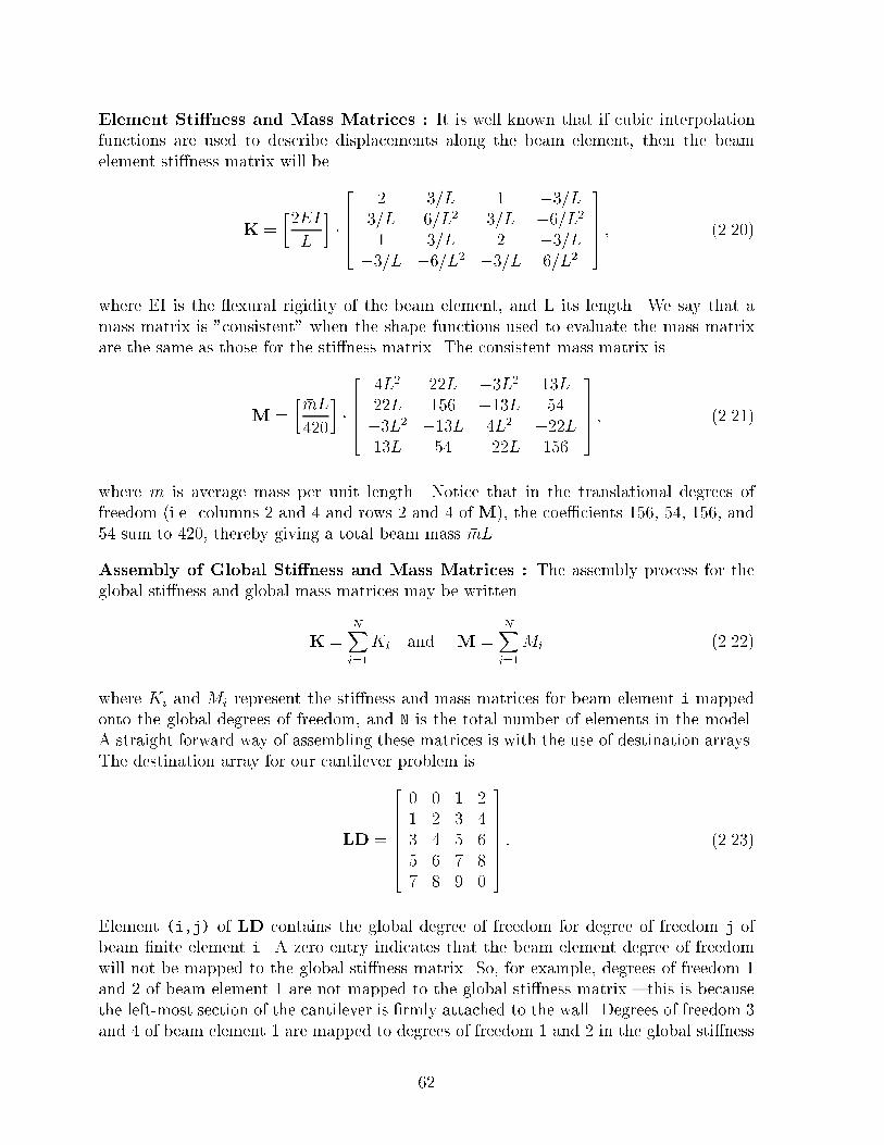
Element Sti�ness and Mass Matrices : It is well known that if cubic interpolationfunctions are used to describe displacements along the beam element, then the beamelement sti�ness matrix will beK = �2EIL � � 26664 2 3=L 1 �3=L3=L 6=L2 3=L �6=L21 3=L 2 �3=L�3=L �6=L2 �3=L 6=L2 37775 ; (2.20)where EI is the exural rigidity of the beam element, and L its length. We say that amass matrix is "consistent" when the shape functions used to evaluate the mass matrixare the same as those for the sti�ness matrix. The consistent mass matrix isM = � �mL420� � 26664 4L2 22L �3L2 13L22L 156 �13L 54�3L2 �13L 4L2 �22L13L 54 �22L 156 37775 ; (2.21)where �m is average mass per unit length. Notice that in the translational degrees offreedom (i.e. columns 2 and 4 and rows 2 and 4 of M), the coe�cients 156, 54, 156, and54 sum to 420, thereby giving a total beam mass �mL.Assembly of Global Sti�ness and Mass Matrices : The assembly process for theglobal sti�ness and global mass matrices may be writtenK = NXi=1Ki and M = NXi=1Mi (2.22)where Ki and Mi represent the sti�ness and mass matrices for beam element i mappedonto the global degrees of freedom, and N is the total number of elements in the model.A straight forward way of assembling these matrices is with the use of destination arrays.The destination array for our cantilever problem isLD = 26666664 0 0 1 21 2 3 43 4 5 65 6 7 87 8 9 037777775 : (2.23)Element (i,j) of LD contains the global degree of freedom for degree of freedom j ofbeam �nite element i. A zero entry indicates that the beam element degree of freedomwill not be mapped to the global sti�ness matrix. So, for example, degrees of freedom 1and 2 of beam element 1 are not mapped to the global sti�ness matrix { this is becausethe left-most section of the cantilever is �rmly attached to the wall. Degrees of freedom 3and 4 of beam element 1 are mapped to degrees of freedom 1 and 2 in the global sti�ness62

and mass matrices. Similarly, degrees of freedom 1, 2, and 3 of beam element 5 will bemapped to global degrees of freedom 7, 8, and 9. Degree of freedom 4 of beam element 5 isnot mapped to the global sti�ness matrix because lateral displacements of the cantileverend are prevented by the hinged support.Details of Input File : A �nite element model for the supported cantilever is de�nedin parts [a] to [f] of the following input �le. The eigenvalue problem is solved in part[g]. ABBREVIATED INPUT FILE/* [a] : Define section/material properties */E = 200000 MPa;I = 15.5E+6 mm^4;L = 4 m;mbar = 31.6 kg/m;/* [b] : Define (4x4) stiffness matrix for beam element */stiff = Matrix([4,4]);stiff = ColumnUnits( stiff, [N, N/m, N, N/m] );stiff = RowUnits( stiff, [m], [1] );stiff = RowUnits( stiff, [m], [3] );stiff[1][1] = 4*E*I/L;stiff[1][2] = 6*E*I/(L^2);stiff[1][3] = 2*E*I/L;stiff[1][4] = -6*E*I/(L^2);stiff[2][1] = 6*E*I/(L^2);stiff[2][2] = 12*E*I/(L^3);stiff[2][3] = 6*E*I/(L^2);stiff[2][4] = -12*E*I/(L^3);stiff[3][1] = 2*E*I/L;stiff[3][2] = 6*E*I/(L^2);stiff[3][3] = 4*E*I/L;stiff[3][4] = -6*E*I/(L^2);stiff[4][1] = -6*E*I/(L^2);stiff[4][2] = -12*E*I/(L^3);stiff[4][3] = -6*E*I/(L^2);stiff[4][4] = 12*E*I/(L^3);PrintMatrix(stiff);/* [c] : Define (4x4) consistent mass matrix for beam element */mass = Matrix([4,4]);mass = ColumnUnits( mass, [ kg*m, kg, kg*m, kg] );mass = RowUnits( mass, [m], [1] );mass = RowUnits( mass, [m], [3] ); 63

mass[1][1] = (mbar*L/420)*4*L*L;mass[2][1] = (mbar*L/420)*22*L;mass[3][1] = (mbar*L/420)*-3*L^2;mass[4][1] = (mbar*L/420)*13*L;mass[1][2] = (mbar*L/420)*22*L;mass[2][2] = (mbar*L/420)*156;mass[3][2] = (mbar*L/420)*-13*L;mass[4][2] = (mbar*L/420)*54;mass[1][3] = (mbar*L/420)*-3*L^2;mass[2][3] = (mbar*L/420)*-13*L;mass[3][3] = (mbar*L/420)*4*L^2;mass[4][3] = (mbar*L/420)*-22*L ;mass[1][4] = (mbar*L/420)*13*L;mass[2][4] = (mbar*L/420)*54;mass[3][4] = (mbar*L/420)*-22*L;mass[4][4] = (mbar*L/420)*156;PrintMatrix(mass);/* [d] : Destination Array beam element connectivity */LD = [ 0, 0, 1, 2 ;1, 2, 3, 4 ;3, 4, 5, 6 ;5, 6, 7, 8 ;7, 8, 9, 0 ];/* [e] : Allocate memory for global mass and stiffness matrices */GMASS = Matrix([9,9]);GMASS = ColumnUnits( GMASS, [ kg*m, kg, kg*m, kg, kg*m, kg, kg*m, kg, kg*m ] );GMASS = RowUnits( GMASS, [m], [1] );GMASS = RowUnits( GMASS, [m], [3] );GMASS = RowUnits( GMASS, [m], [5] );GMASS = RowUnits( GMASS, [m], [7] );GMASS = RowUnits( GMASS, [m], [9] );GSTIFF = Matrix([9,9]);GSTIFF = ColumnUnits( GSTIFF, [ N, N/m, N, N/m, N, N/m, N, N/m, N ] );GSTIFF = RowUnits( GSTIFF, [m], [1] );GSTIFF = RowUnits( GSTIFF, [m], [3] );GSTIFF = RowUnits( GSTIFF, [m], [5] );GSTIFF = RowUnits( GSTIFF, [m], [7] );GSTIFF = RowUnits( GSTIFF, [m], [9] );/* [f] : Assemble Global Stiffness/Mass Matrices for Two Element Cantilever */no_elements = 5;for( i = 1; i <= no_elements; i = i + 1) {for( j = 1; j <= 4; j = j + 1) { 64

row = LD [i][j];if( row > 0) {for( k = 1; k <= 4; k = k + 1) {col = LD [i][k];if( col > 0) {GMASS [ row ][ col ] = GMASS [ row ][ col ] + mass[j][k];GSTIFF[ row ][ col ] = GSTIFF[ row ][ col ] + stiff[j][k];}}}}}/* [g] : Compute and Print Eigenvalues and Eigenvectors */no_eigen = 2;eigen = Eigen( GSTIFF, GMASS, [ no_eigen ]);eigenvalue = Eigenvalue(eigen);eigenvector = Eigenvector(eigen);for(i = 1; i <= no_eigen; i = i + 1) {print "Mode", i ," : w^2 = ", eigenvalue[i][1];print " : T = ", 2*PI/sqrt(eigenvalue[i][1]) ,"\n";}PrintMatrix(eigenvector);Points to note are:[1] Element level sti�ness matrices are stored in stiff. Rows 1 and 3 of stiff representequations of equilibrium when a moment is applied at the beam end to cause a unitrotation, and rows 2 and 4, equations of equilibrium for unit lateral displacementsof the beam element. We distinguish these cases by applying units of m to rows 1and 3.[2] Element level mass matrices are stored in mass. By de�nition, terms in the massmatrix correspond to forces, or torques, required to cause unit translational orrotational acceleration. A unit acceleration in a translational degree of freedom willrequire a force of the type force = mass � acc'n, with mass taking kilogram (kg)units. A unit rotational acceleration will have the form torque = inertia � angularacc'n. The units for inertia are kg m2.[3] The (9�9) global mass and global sti�ness matrices are stored in GMASS and GSTIFF,respectively. The statements row = LD[i][j] and col = LD[i][j] contain therow-column mapping for the beam element degrees of freedom onto the global de-grees of freedom. 65

Abbreviated Output File : Details of the beam element sti�ness and mass matrices,and ensuing eigenvalues and eigenvectors are as follows:START OF ABBREVIATED OUTPUT FILEMATRIX : "stiff"row/col 1 2 3 4units N N/m N N/m1 m 3.10000e+06 1.16250e+06 1.55000e+06 -1.16250e+062 1.16250e+06 5.81250e+05 1.16250e+06 -5.81250e+053 m 1.55000e+06 1.16250e+06 3.10000e+06 -1.16250e+064 -1.16250e+06 -5.81250e+05 -1.16250e+06 5.81250e+05MATRIX : "mass"row/col 1 2 3 4units kg.m kg kg.m kg1 m 1.92610e+01 2.64838e+01 -1.44457e+01 1.56495e+012 2.64838e+01 4.69486e+01 -1.56495e+01 1.62514e+013 m -1.44457e+01 -1.56495e+01 1.92610e+01 -2.64838e+014 1.56495e+01 1.62514e+01 -2.64838e+01 4.69486e+01*** SUBSPACE ITERATION CONVERGED IN 7 ITERATIONSMode 1.0000e+00 : w^2 = 145.8 rad.sec^-2.0 : T = 0.5203 secMode 2.0000e+00 : w^2 = 1539 rad.sec^-2.0 : T = 0.1602 secMATRIX : "eigenvector"row/col 1 2units1 1.24900e-01 -2.28500e-012 m 3.02715e-01 -7.71256e-013 1.03061e-01 1.77895e-014 m 8.01556e-01 -9.46803e-015 -1.29310e-02 3.44764e-016 m 1.00000e+00 3.03399e-017 -1.37281e-01 -5.51890e-028 m 6.87189e-01 1.00000e+009 -1.89640e-01 -3.58198e-01Points to note are:[1] The eigenvalues of this problem correspond to the circular natural frequency squaredof the individual modes, and they take the units rad/sec/sec. The natural periodof vibration for the �rst and second modes is 0.5203 seconds, and 0.1602 seconds,respectively.[2] The �rst two eigenvectors are summarized in the script of abbreviated output. Per-haps the most surprising result of this analysis is the unit on the eigenvectors { for66

MODE 1 : PERIOD = 0.5203 SECONDS

-1

1 1

-1

MODE 2 : PERIOD = 0.1602 SECONDSFigure 2.6: Mode Shapes and Periods of Vibration for Single Span Steel Beamthose degrees of freedom corresponding to translational displacements, the eigen-vector is printed with units of length. The remaining degrees of freedom representrotations, and take the (non-dimensional) units of radians.[3] Figure 2.6 shows the mode shapes and natural periods of vibration for the supportedcantilever beam. We have drawn the mode shapes as connected straight lines {actually, the mode shapes will be cubic splines, as de�ned by the beam elementshape functions.

67

Chapter 3Construction of NumericalAlgorithms3.1 IntroductionThe purpose of this chapter is to test the exibility of ALADDIN's commandlanguage by constructing basic numerical algorithms for computing the roots of nonlinearequations, and the minima of multi-dimensional functions subject to linear and nonlinearconstraints. We have selected this problem domain because the numerical algorithmsmay be incorporated into �nite element analyses of linear and nonlinear structures. Fordetails, see Chen and Austin [10].3.2 Roots of Nonlinear EquationsLet x = (x1; x2; � � � ; xn)T by a coordinate point in n-dimensional space, and f =(f1; f2; � � � ; fn)T be a n-dimensional (nonlinear) vector. The roots of nonlinear equationsf are given by solutions to f(x) = 0: (3.1)3.2.1 Newton-Raphson and Secant AlgorithmsThe methods of Newton-Raphson and Secant Approximation are among themost popular for computing the roots of nonlinear equations. Let vector xo be an initialguess at the solution to equation (3.1). The method of Newton-Raphson corresponds toa sequence of �rst order Taylor series expansion about x(k), namelyf(x(k+1)) = f(x(k)) +rf(x(k)) � (x(k+1) � x(k)) � 068

f(x)

f(x) = 0

f (

x_o

)

f( x_1 )

x_o x__1 x_2 x_3

f ( x_2 )

f ( x_3 )

Figure 3.1: Secant Approximation of Quasi-Newton Methodwhere k = 0, 1, 2, � � �, n, and (rf(x))ij = (@fi)=(@xj). In matrix form, the gradientapproximation is rf(x) = 2666664 @f1(x)@x1 @f1(x)@x2 � � � @f1(x)@xn@f2(x)@x1 @f2(x)@x2 � � � @f2(x)@xn� � � � � � � � � � � �@fn(x)@x1 @fn(x)@x2 � � � @fn(x)@xn3777775 : (3.2)If rf(x(k)) has an inverse, then the (full) Newton-Raphson update is:x(k+1) = x(k) � hf(x(k))i�1 � rf(x(k)): (3.3)The procedure is repeated until convergence criteria are satis�ed. While the method offull Newton-Raphson can be e�cient in some speci�c nonlinear analyses, Bathe [7, 9]reports that in general, full Newton-Raphson is not a competitive computational methodfor computing the roots of a wide-range of nonlinear equations. A major limitation of fullNewton-Raphson is the need for updating and factorizing the coe�cient matrix -rf(x(k))at each iteration. One strategy for avoiding these computationally expensive steps isto replace -rf(x(k)) in equation (3.3) with -rf(x(0)), thereby eliminating the need torecalculate and factorize -rf(x(k)) at each iteration. From a mathematical point of view,this simpli�cation corresponds to a linearization of the gradient f(xo). For problems withsigni�cant nonlinearities { in particular when the system sti�ens during the response {this linearization can lead to a very slow convergence in the iteration. Even worse, theiteration may diverge.The class of quasi-Newton methods are a second alternative to full Newton Raph-69

son. Quasi-Newton methods update the coe�cient matrix, or it's inverse, to provide asecant approximation to the matrix from iteration (k) to (k+1). Figure 3.1 shows, forexample, a sequence of secant approximations one might apply during the computationof roots in a one-dimension nonlinear equation. If a displacement increment is de�ned�(k+1) = x(k+1) � x(k) (3.4)an increment in the residuals de�ned as (k+1) = f(x(k))� f(x(k+1)); (3.5)then the updated secant sti�ness matrix, K(k+1), will satisfy the quasi-Newton equationK(k+1)�(k+1) = (k+1).3.2.2 Broyden-Fletcher-Goldfarb-Shanno (BFGS) AlgorithmAmong Quasi-Newton methods, the Broyden-Fletcher-Goldfarb-Shanno (BFGS)method appears to be the most e�ective. Within iteration (k+1), the BFGS methodemploys the following procedure to evaluate x(k+1) and K(k+1) [9]:Step 1 : Initialization. Provide an initial value of vector x = x0, and calculate thecorresponding Ko matrix at x = xo.Step 2 : Evaluated the x vector increment�x = �hf(x(k))i�1 � rf(x(k)): (3.6)This vector increment de�nes a direction for the actual increment.Step 3 : Perform a line-search along direction �x to satisfy \equilibrium." Details ofthe line-search are as follows. First, set � = 1:0 and let the x vectorx(k+1) = x(k) + ��x (3.7)where � is a scalar multipler. The product � j �x j represents the distance between pointsx(k) and x(k+1). The value of � is changed until the component of the residual in direction�x, as de�ned by the inner product of �xTf(x(k+1)), is approximately zero. The lattercondition is satis�ed when�xT � f(x(k+1)) � STOL ��xT � f(x(k)): (3.8)STOL is a convergence tolerance. The distance of the line search is automatically halvedafter each failure of equation (3.8) by halving �; x(i) is then recalculated with the new70

�. If after �ve or ten line search attempts, equation (3.8) still isn't satis�ed, then thedirection given by the �x is probablely wrong. A new direction calculation is needed.This procedure is summarized in four-substeps:Step 3.1 : Use equation (3.6) to update x.Step 3.2 : Begin while loop : While equation (3.8) is not satis�ed, work throughSubsteps 3.3 to 3.5.Step 3.3 : If the line search number is less than or equal to MaxLineSearchCount, thenset � = �=2:0, and use equation (3.6) to update x.Step 3.4 : If the line search number is greater than MaxLineSearchCount, then breakthe while loop. Recalculate matrix K at x = x(k+1). Go to Step 2.Step 3.5 : End while loop : Go to Step 4 for BFGS update.Step 4 : Use equations (3.4) and (3.5) to calculate �(k+1) and (k+1).Step 5 : Use the BFGS update [9] to revise the inverse of coe�cient matrix K. Theupdate of K is given by K�1(k+1) = A(k+1)TK�1(k)A(k+1) (3.9)where the matrix A(k+1) is a (n� n) matrixA(k+1) = I + v(k+1) � w(k+1)T : (3.10)Vectors v(k+1) and w(k+1) are given byv(k+1) = � " �(k+1)T (k+1)�(k+1)T�f(x(k))# � � � f(x(k))� (k+1) (3.11)and w(k+1) = " �(k+1)�(k+1)T (k+1)# : (3.12)Step 6 : To avoid numerically dangerous updates, the conditional numberc(k+1) = " �(k+1)T (k+1)�(k+1)T�f(x(k))#1=2 (3.13)of the updating matrix A(k+1) must be compared to some predetermined tolerance. Alarge condition number implies that the updated inverse matrix will be nearly singular.Numerical updates are not performed if the condition number exceeds this tolerance { inthis project, we follow the recommendation of Bathe [9], and set the tolerance at 105.71

Step 7 : Check convergence of force and energy equilibriums. The force convergencecriterion requires that the norm of the out-of-balance residual or force to be within apre-set tolerance �F of the �rst residual.kf(x(k+1))k2 � �F � kf(x(o))k (3.14)A force criterion is not su�cient to ensure convergence. Consider the case of functionf(x) with small or closing to zero gradients, the out-of-balance residual or force may bevery small while the variable x or displacement may be grossly in error. Therefore, the\energy equilibrium" condition is necessary to provide the indication that both �x(k+1),and residual are approaching zeros. It requires computation of the work done by the forceresidual moving through displacement increment �x.�x(k+1) � f(x(k)) � �E ��x(o) � f(x(0)) (3.15)where the �E is a preset energy tolerance. In the following examples, we will use �F = 10�4and �E = 10�5.Numerical Example : We demonstrate use of the BFGS algorithm by solving a two-variable family of nonlinear equations:2x12 + x2 = 4x1 + 2x22 = 5 (3.16)These equations may also be written fFg � fRg = 0, wherefFg = ( 2x12 + x2x1 + 2x22 ) fRg = ( 45 ) (3.17)We use the parameter MaxLineSearchCount = 5 for the maximum number for line searchtrials, and select an initial trial vector fxg = (7; 10)T .START OF INPUT FILE/** =====================================================* Use BFGS Algorithm to Solve Nonlinear Equations** Function :* 2x[1]^2 + x[2] = 4* x[1] + 2x[2]^2 = 5** R^t = (4, 5)* F[1] = 2x[1]^2 + x[2]* F[2] = x[1] + 2x[2]^2* K[i][j] = dF[i]/dx[j] Jacobain matrix** Written By : X.G. Chen June 1994* =====================================================72

*/dimen = 2;IMAX = 20; /* Maximum number of iteration */Ef = 1E-4;Ee = 1.E-5;beta = 1.0;STOL = 0.5;EPS = 1.E-5;ii = 1;MaxLineSearchCount = 5;/* [a] : Initialize and print problem parameters and initial solution */x = [7; 10];R = [4; 5];print "------initial Guess -----\n";PrintMatrix(x);print "\n------Given R value -----\n";PrintMatrix(R);Y = [2*x[1][1], 1; 1, 2*x[2][1]];K = [4*x[1][1], 1; 1, 4*x[2][1]];F = Y*x;Residu0 = R-F;Residu = R-F;K_inver = Inverse(K);/* [b] : Allocate working matrices */Residu_old = Residu;I = Diag([dimen, 1]);delta_old = Zero([dimen, 1]);/* [c] : Main Loop for Iteration */Iter_no = 0;for (ii = 1; ii <= IMAX; ii = ii + 1) {Iter_no = Iter_no + 1;beta = 1.0;delta = K_inver*Residu;/* [c.1] : Armijo Line Search */x_temp = x + beta*delta;temp1 = QuanCast(Trans(delta)*Residu);Y = [2*x_temp[1][1], 1; 1, 2*x_temp[2][1]];F = Y*x_temp;Residu = R- F;temp2 = QuanCast(Trans(delta)*Residu);counter = 0;while(temp2 > temp1*STOL + EPS) { 73

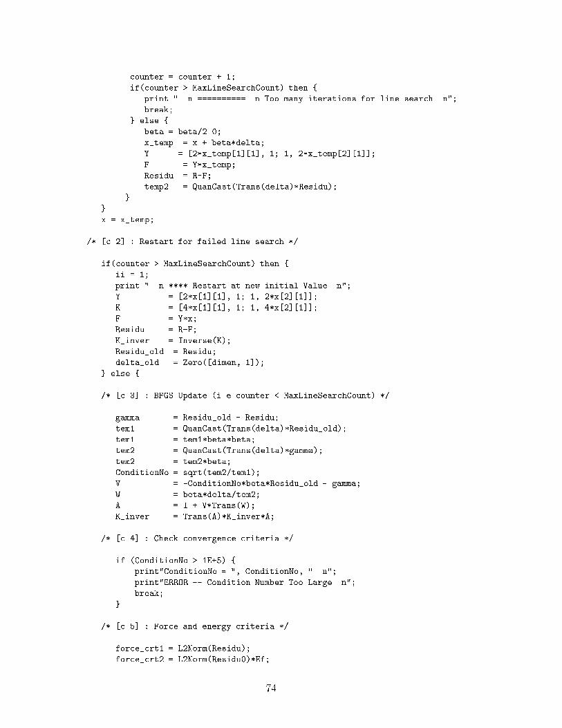
counter = counter + 1;if(counter > MaxLineSearchCount) then {print " \n ========== \n Too many iterations for line search \n";break;} else {beta = beta/2.0;x_temp = x + beta*delta;Y = [2*x_temp[1][1], 1; 1, 2*x_temp[2][1]];F = Y*x_temp;Residu = R-F;temp2 = QuanCast(Trans(delta)*Residu);}}x = x_temp;/* [c.2] : Restart for failed line search */if(counter > MaxLineSearchCount) then {ii = 1;print " \n **** Restart at new initial Value \n";Y = [2*x[1][1], 1; 1, 2*x[2][1]];K = [4*x[1][1], 1; 1, 4*x[2][1]];F = Y*x;Residu = R-F;K_inver = Inverse(K);Residu_old = Residu;delta_old = Zero([dimen, 1]);} else {/* [c.3] : BFGS Update (i.e counter < MaxLineSearchCount) */gamma = Residu_old - Residu;tem1 = QuanCast(Trans(delta)*Residu_old);tem1 = tem1*beta*beta;tem2 = QuanCast(Trans(delta)*gamma);tem2 = tem2*beta;ConditionNo = sqrt(tem2/tem1);V = -ConditionNo*beta*Residu_old - gamma;W = beta*delta/tem2;A = I + V*Trans(W);K_inver = Trans(A)*K_inver*A;/* [c.4] : Check convergence criteria */if (ConditionNo > 1E+5) {print"ConditionNo = ", ConditionNo, " \n";print"ERROR -- Condition Number Too Large \n";break;}/* [c.5] : Force and energy criteria */force_crt1 = L2Norm(Residu);force_crt2 = L2Norm(Residu0)*Ef;74

energy_crt1 = QuanCast(Trans(delta)*Residu_old);energy_crt1 = abs(energy_crt1);if (ii == 1) {energy_crt2 = QuanCast(Trans(delta)*Residu0);energy_crt2 = abs(energy_crt2*Ee);}if((force_crt1 <= force_crt2) && (energy_crt1 < energy_crt2)) {break;}Residu_old = Residu;delta_old = delta;}}/* [d] : Print results and terminate program execution */print" \n RESULTS : \n --------------\n";print" Iteration Number =", Iter_no, "\n";Y = [2*x[1][1], 1; 1, 2*x[2][1]];F = Y*x;PrintMatrix(x, F);quit;The program output is------initial Guess -----MATRIX : "x"row/col 1units1 7.00000e+002 1.00000e+01------Given R value -----MATRIX : "R"row/col 1units1 4.00000e+002 5.00000e+00==========Too many iterations for line search**** Restart at new initial Value 75

RESULTS :--------------Iteration Number = 1.0000e+01MATRIX : "x"row/col 1units1 1.14237e+002 1.38883e+00MATRIX : "F"row/col 1units1 3.99883e+002 5.00004e+00

76

3.3 Han-Powell Algorithm for OptimizationIn this section we will demonstrate how ALADDIN can be used to solve a seriesof optimization problems. Before we get to the details of the input �le, we will brie ydescribe the Han-Powell algorithm for optimization.Let x be a n-dimensional vector, f(x) a n-dimensional function, and g(x) a m-dimensional function. The purpose of this section is to solve the mathematical problemminimize f(x)subject to g(x) = 0 (3.18)by constructing a quadratic programming (QP) method, combined with an Armijo linesearch procedure, and Han-Powell's method of modi�ed BFGS update (mathematicaldescriptions of these algorithms can be found in Luenberger [22]).We begin by recalling that the Lagrange �rst-order necessary conditions for thisproblem amounts to solving the system of equationsrf(x) + �Trg(x) = 0g(x) = 0 (3.19)for x and �. In terms of Lagrange function, above equation can be written asrl(x; �) = 0g(x) = 0where l(x; �) = f(x) + g(x)�, and � is the Lagrange multiplier.3.3.1 Quadratic Programming (QP)The quadratic programming method is based on two mathematical assumptions,namely:[1] Assume that the objective function f(x)may be approximated by a quadratic equationde�ned by a second order Taylor's series expansion about xk.[2] Assume that solutions to the constraint equation g(x) = 0 are approximately givenby a �rst order Taylors expansion about xk.Together, these assumptions implyf(xk+1) � f(xk) +rf(xk)Td+ 12dTBkd77

g(xk+1) � g(xk) +rg(xk)TdThe optimization problem described by equation (3.18) can be approximated by the fol-lowing quadratic program problemminimize rf(xk)Td+ 12dTBkdsubject to g(xk) +rg(xk)Td = 0 (3.20)where d = x�xk, and Bk is the Hessian of function f(x). Langrange's necessary conditionsare Bkd+rg(xk)�+rf(xk) = 0g(xk) +rg(xk)Td = 0: (3.21)and in this particular case, comprise an (n+m) dimensional linear system of equations. IfBk is positive de�nite, and rg(x) has rank of m, then the matrix" Bk rg(xk)rg(xk)T 0 #is nonsingular [22], and equations (3.21) may be solved with unique solutions" Bk rg(xk)rg(xk)T 0 # " d� # = " �rf(xk)�g(xk) # (3.22)to d and �. The abovementioned QP solver gives the direction d for the next step. Wewill use the Armijo line search rule to determine how far an algorithm should move alongthis direction.3.3.2 Armijo Line Search RuleThe essential idea is that the rule should �rst guarantee that the selected t is nottoo large. Let us de�ne the function�(t) = f(xk + t dk)for �xed � and t = (1; �; �2; �3; � � � ), a value of t is considered to be not too large if thecorresponding function value lies below the dashed line; that is, if�(t) � �(0) + ��0(0) t (3.23)In this example, we chose � = 0:1; � = 0:5.78

3.3.3 The BFGS update and Han-Powell methodFor the problem with equality constraints described in equation (3.19), the struc-tured Newton method can be applied. We consider the iterative process de�ned by:" xk+1�k+1 # = " xk�k #� " Bk rg(xk)rg(xk)T 0 #�1 " rf(xk; �k)Tg(xk) # (3.24)Let yk = " xk� # Ak = " B rg(xk)rg(xk)T 0 # Ck = " rf(xk; �)Tg(xk) #Notation for equation (3.24) can be simpli�ed as:yk+1 = yk � A�1k CkThe top part of system (3.22) can be rewritten as:Bkd = �rf(xk)T �rg(xk)� = �rl(xk; �) (3.25)and equation (3.25) can be implemented as a quasi-Newton method, with updates ofmatrix B Bk+1 = Bk + qkqTkqTk pk � BkpkpTkBkpTkBkpk ; (3.26)used to approximate the hessian of the lagrangian. In equation (3.26) pk = xk+1 � xkand qk = rl(xk+1; �k+1)T � rl(xk; �k+1)T . The Lagrange multiplier is calculated fromsolutions to (3.25). To ensure Bk remains positive de�nite, the standard BFGS update isslightly altered.The Han-Powell Method: The method consists of the following steps:Step 1 : Start with an initial point x0 and an initial positive de�nite matrix bf B0 , setk = 0.Step 2 : Solve the quadratic program described by system (3.20). If d = 0 is a solution,then the current point satis�es the �rst order necessary conditions for a solution to theoriginal problem (3.19).Step 3 : With d found above, perform a line search in the direction d.Step 4 : Update Bk, according to 79

Bk+1 = Bk � BkpkpTkBkpTkBkpk + rkrTkpTk rk (3.27)pk = xk+1 � xk (3.28)qk = rl(xk+1; �k+1)�rl(xk; �k) (3.29)rk = �kqk + (1� �k)Bkpk (3.30)where �k+1 is the language multiplier vector of (3.20), and where�k = 8>><>>: 1 if pTk qk � (0:2)pTkBkpk(0:8)pTk BkpkpTkBkpk�pTk qk if pTk qk < (0:2)pTkBkpk: (3.31)Again, detailed discussion on this method can be found in [22]Numerical Examples : Consider the following three problems:Example 1 : Minimize a quadratic function with a set of linear constraints.minimize : f(x) = (x1 � x2)2 + (x2 + x3 � 2)2 + (x4 � 1)2 + (x5 � 1)2subject to: g1(x) = x1 + 3x2 � 4 = 0g2(x) = x3 + x4 � 2x5 = 0g3(x) = x2 � x5 = 0 (3.32)Example 2 : Minimize a nonlinear non-quadratic function with a set of linear constraints.minimize : f(x) = (x1 � 1)2 + (x1 � x2)2 + (x2 � x3)4subject to: g1(x) = x1 + x2 + 2x3 � 4 = 0g2(x) = x1 + x3 � 2 = 0 (3.33)Example 3 : Minimize a nonlinear non-quadratic function with nonlinear constraint.minimize : f(x) = (x1 � 1)2 + (x1 � x2)2 + (x2 � x3)4subject to: g(x) = x1(1 + x22) + x43 � 3 = 0 (3.34)It is not di�cult to observe that the analytical solution to the above examples are x =(1, 1, 1, 1, 1), x = (1,1,1) and x = (1, 1, 1).Since the input commands for above examples are basically same except for thefunctions, we only illustrate one command �le for example 1. But we give all the resultsfor example 1, 2 and 3. START OF INPUT FILE80

/** ================================================================* Example Problem 1:** minmize f(x) = (x1 -x2)^2 + (x2+x3-2)^2 + (x4-1)^2 + (x5 -1)^2** Subject to constraints:** x1+3*x2 -4 = 0* x3+x4-2*x5 = 0* x2 -x5 = 0** Notation -- f = f(x), G = g(x), Df = grad f(x), Dg = grad g(x).** Written By: X.G. Chen June 1994* ================================================================*/SetUnitsOff;/* [a] : Initialize and print variables and matrices */Epsilon = 1E-6;beta = 0.5;alpha = 0.1;IMAX = 20; /* maximum of iterations */n = 5; /* number of variables */M = 3; /* number of constraints */print "\n ****** Initial Guess Value ******* \n";x = [20; 0.1; 10; -1; -10]; /* not feasible */PrintMatrix(x);x_old = x;lambda = Zero([M, 1]);lambda_old = Zero([M, 1]);temp1 = (x[1][1] -x[2][1])*(x[1][1] -x[2][1]);temp2 = (x[2][1] +x[3][1] -2)*(x[2][1] +x[3][1] - 2);temp3 = (x[4][1] -1)*(x[4][1] -1);temp4 = (x[5][1] -1)*(x[5][1] -1);f = temp1 + temp2 + temp3 + temp4;A = Zero([n+M, n+M]);C = Zero([n+M, 1]);B = Zero([n,n]);Df = Zero([n,1]);DF = Zero([n,1]);b = Zero([M,1]);d = Zero([n,1]);Df[1][1] = 2*(x[1][1]- x[2][1]);Df[2][1] = -2*(x[1][1]- x[2][1]) + 2*(x[2][1]+ x[3][1] -2);Df[3][1] = 2*(x[2][1]+ x[3][1]-2); 81

Df[4][1] = 2*(x[4][1]- 1);Df[5][1] = 2*(x[5][1]- 1);B = Diag([n,1]); /* initialize B as identity matrix */b[1][1] = -4;b[2][1] = 0;b[3][1] = 0;k = 1;Trans_Dg = [1,3,0,0,0; 0,0,1,1,-2; 0, 1, 0, 0,-1];Dg = Trans(Trans_Dg);G = Trans_Dg*x+b;/* [b] : Initialize matrices A and C */for ( i = 1; i <= n+M; i = i + 1) {for(j = 1; j <= n + M; j = j + 1) {if( i <= n) then {C[i][1] = -Df[i][1];if(j <= n) then {A[i][j] = B[i][j];} else {k = j - n;A[i][j] = Dg[i][k];}} else {k = i - n;C[i][1] = -G[k][1];if(j <= n) {A[i][j] = Trans_Dg[k][j];}}}}q = Zero([n,1]);/* [c] : Main Loop */for ( ii = 1; ii <= IMAX; ii = ii + 1 ) {/* [c.1] : Solve QP for direction d */y = Solve(A,C);for ( i = 1; i <= n; i = i + 1) {d[i][1] = y[i][1];}for ( i = n+1; i <= n+M; i = i + 1) {j = i-n;lambda[j][1] = y[i][1];} 82

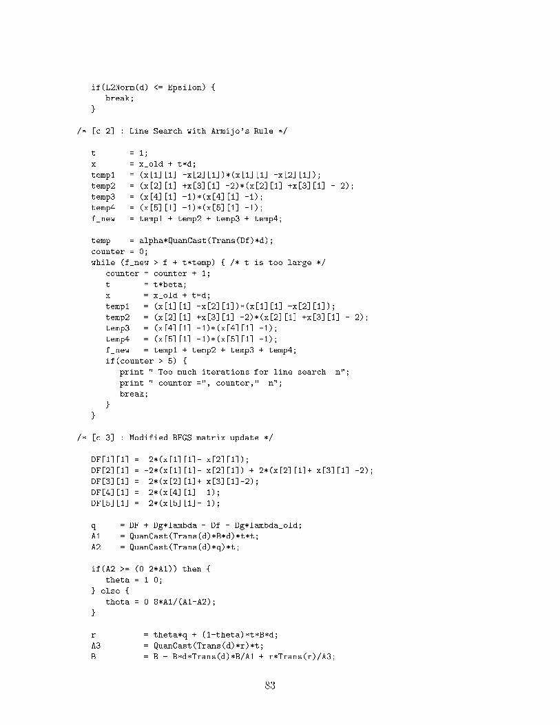
if(L2Norm(d) <= Epsilon) {break;}/* [c.2] : Line Search with Armijo's Rule */t = 1;x = x_old + t*d;temp1 = (x[1][1] -x[2][1])*(x[1][1] -x[2][1]);temp2 = (x[2][1] +x[3][1] -2)*(x[2][1] +x[3][1] - 2);temp3 = (x[4][1] -1)*(x[4][1] -1);temp4 = (x[5][1] -1)*(x[5][1] -1);f_new = temp1 + temp2 + temp3 + temp4;temp = alpha*QuanCast(Trans(Df)*d);counter = 0;while (f_new > f + t*temp) { /* t is too large */counter = counter + 1;t = t*beta;x = x_old + t*d;temp1 = (x[1][1] -x[2][1])*(x[1][1] -x[2][1]);temp2 = (x[2][1] +x[3][1] -2)*(x[2][1] +x[3][1] - 2);temp3 = (x[4][1] -1)*(x[4][1] -1);temp4 = (x[5][1] -1)*(x[5][1] -1);f_new = temp1 + temp2 + temp3 + temp4;if(counter > 5) {print " Too much iterations for line search \n";print " counter =", counter," \n";break;}}/* [c.3] : Modified BFGS matrix update */DF[1][1] = 2*(x[1][1]- x[2][1]);DF[2][1] = -2*(x[1][1]- x[2][1]) + 2*(x[2][1]+ x[3][1] -2);DF[3][1] = 2*(x[2][1]+ x[3][1]-2);DF[4][1] = 2*(x[4][1]- 1);DF[5][1] = 2*(x[5][1]- 1);q = DF + Dg*lambda - Df - Dg*lambda_old;A1 = QuanCast(Trans(d)*B*d)*t*t;A2 = QuanCast(Trans(d)*q)*t;if(A2 >= (0.2*A1)) then {theta = 1.0;} else {theta = 0.8*A1/(A1-A2);}r = theta*q + (1-theta)*t*B*d;A3 = QuanCast(Trans(d)*r)*t;B = B - B*d*Trans(d)*B/A1 + r*Trans(r)/A3;83

Df = DF;x_old = x;lambda_old = lambda;G = Trans_Dg*x+b;for ( i = 1; i <= n; i = i + 1) {C[i][1] = -Df[i][1];for(j = 1; j <= n; j = j + 1) {A[i][j] = B[i][j];}}for ( i = 1; i <= M; i = i + 1) {k = i + n;C[k][1] = -G[i][1];}}/* [d] : Print results and terminate program execution */print" Results: \n --------------\n";print" Iteration Number =", ii-1, "\n\n";PrintMatrix(x);quit;If B is initialized with identity matrix, then the results are:Example 1:****** Initial guess value *******MATRIX : "x"row/col 11 2.00000e+012 1.00000e-013 1.00000e+014 -1.00000e+005 -1.00000e+01Results:--------------Iteration Number = 10MATRIX : "x"row/col 11 1.00000e+002 1.00000e+003 1.00000e+004 1.00000e+005 1.00000e+00 84

Example 2:****** Initial guess value *******MATRIX : "x"row/col 1units1 2.00000e+002 2.00000e+003 2.00000e+00Results:--------------Iteration Number = 5.0000e+00MATRIX : "x"row/col 1units1 9.99891e-012 9.99891e-013 1.00011e+00Example 3: The process will not converge after maximum number of twenty iterations.And increase maximum number can not help the convergence.****** Initial guess value *******MATRIX : "x"row/col 11 2.00000e+002 1.40000e+003 1.50000e+00Results:--------------Iteration Number = 2.0000e+01MATRIX : "x"row/col 11 1.00032e+002 1.01113e+003 9.94158e-01If B is initialized with B(x0), then the results are:Example 1:****** Initial guess value *******MATRIX : "x" 85

row/col 11 2.00000e+012 1.00000e-013 1.00000e+014 -1.00000e+005 -1.00000e+01Results:--------------Iteration Number = 1.0000e+00MATRIX : "x"row/col 11 1.00000e+002 1.00000e+003 1.00000e+004 1.00000e+005 1.00000e+00Example 2:****** Initial guess value *******MATRIX : "x"row/col 1units1 2.00000e+002 2.00000e+003 2.00000e+00Results:--------------Iteration Number = 1.0000e+00MATRIX : "x"row/col 1units1 1.00000e+002 1.00000e+003 1.00000e+00Example 3:****** Initial guess value *******MATRIX : "x"row/col 11 2.00000e+002 1.40000e+003 1.50000e+00Results:-------------- 86

Iteration Number = 6.0000e+00MATRIX : "x"row/col 11 9.99850e-012 9.94974e-013 1.00240e+00In these three examples, the hessian of f(x) is stored in matrix B. The hessian is constant.Moreover, when the B matrix corresponds to the exact value, only one iteration of opti-mization is required to compute an optimal solution. The initial guess point for Example2 is a feasible point. While the points for Example 1 and 3 are not feasible points.

87

Chapter 4Computational Methods forDynamic Analysis of Structures4.1 IntroductionIn this section we demonstrate how ALADDIN may be used to compute the time-history response of a linear elastic multi-degree of freedom system de�ned by the equationof equilibrium M �X(t) +C _X(t) +KX(t) = P(t): (4.1)In equation (4.1)M, C, and K are (n�n) mass, damping, and sti�ness matrices, respec-tively. P(t), X(t), _X(t), and �X(t) are (n � 1) external load, displacement, velocity, andacceleration vectors at time t.Two numerical procedures are described and demonstrated in this chapter. Webegin with the method of Newmark Integration to compute the time-history response ofa four story shear structure. Then we repeat the analysis using the method of ModalAnalysis. In both cases, the shear structure is acted upon by a saw-toothed external forceapplied to the roof-level degree of freedom.4.2 Method of Newmark IntegrationNewmark integration methods [8] approximate the time dependent response oflinear and nonlinear 2nd-order equations by insisting that equilibrium be satis�ed only ata discrete number of points (or timesteps). If (t) and (t+4t) are successive timesteps inthe integration procedure, the two equations of equilibrium that must be satis�ed areM �X(t) +C _X(t) +KX(t) = P(t); (4.2)and 88

M �X(t+4t) +C _X(t+4t) +KX(t+4t) = P(t+4t): (4.3)Now let's assume that solutions to equation (4.2) are known, and (4.3) needs to be solved.At each timestep there are 3n unknowns corresponding to the displacement, velocity,and acceleration of each component of X. Since we only have n equations, the naturalrelationship existing between the acceleration and velocity,_X(t +4t) = _X(t) + R (t+4t)(t) �X(�)d�; (4.4)and velocity and displacementX(t +4t) = X(t) + R (t+4t)(t) _X(�)d�; (4.5)must be enforced to reduce the number of unknowns to n. �X(�) is an unknown function forthe acceleration across the timestep. The Newmark family of integration methods assumethat: (1) acceleration within the timestep behaves in a prescribed manner, and (2) theintegral of acceleration across the timestep may be expressed as a linear combination ofaccelerations at the endpoints. Discrete counterparts to the continuous update in velocityand displacement are:_X(t+4t) = _X(t) +4th(1� ) �X(t) + �X(t+4t)i (4.6)X(t+4t) = X(t) +4t _X(t) + 4t22 h(1� 2�) �X(t) + 2� �X(t+4t)i (4.7)with the parameters and � determining the accuracy and stability of the method un-der consideration. The equations for discrete update in velocity and displacement aresubstituted into equation (4.3) and rearranged to give:M̂ �X(t+4t) = P̂(t +4t) (4.8)where M̂ =M + 4tC+ �4t2K (4.9)and P̂(t+4t) = P(t+4t)�C _X(t)�KX(t)�4t [K] _X(t)�4th(1� )C+ 4t2 (1� 2�)Ki �X(t): (4.10)It is well known that when = 1=2 and � = 1=4, acceleration is constant within thetimestep t 2 [t; t+4t], and equal to the average of the endpoint accelerations. In such89

cases, approximations to the velocity and displacement will be linear and parabolic, re-spectively. Moreover, this discrete approximation is second order accurate and uncon-ditionally stable. It conserves energy exactly for the free response vibration of linearundamped SDOF systems (we will check for conservation of energy in the numerical ex-amples that follow).Numerical Example : The method of Newmark Integration is demonstrated by comput-ing the time-history response of the four story building structure caused by a time-varyingexternal load applied to the roof level. Details of the shear building and external loadingare shown in Figures 4.1 and 4.3.

k_4 = 1600 kN/m.

k_3 = 1200 kN/m.

k_2 = 800 kN/m.

k_1 = 400 kN/m.

MASS = 1500 kg.

MASS = 3000 kg

MASS = 3000 kg

MASS = 4500 kg

k_3 = 1200 kN/m.

k_2 = 800 kN/m.

k_1 = 400 kN/m.

k_4 = 1600 kN/m.

x_1

x_2

x_3

x_4

800

-800 2400

-800

-1600

-1600

4000

-2400 5600

STIFFNESS =

MASS =

1500

3000

3000

4500

kN/m.

kg

-2400

Figure 4.1: Schematic of Shear Building for Newmark AnalysisA simpli�ed model of the building is obtained by assuming that all of the building massis lumped at the oor levels, that the oor beams are rigid, and that the columns areaxially rigid. Together these assumptions generate model that is commonly known as ashear-type building model, where displacements at each oor level may be described byone degree-of-freedom alone. Only four degrees of freedom are needed to describe totaldisplacements of the structure.Details of the mass and sti�ness matrices are shown on the right-hand side of Fig-ure 4.1. From a physical point of view, element (i,j) of the sti�ness matrix correspondsto the nodal force that must be applied to degree of freedom j in order to produce aunit displacement at degree of freedom i, and zero displacements at all other degrees offreedom. 90

Figure 4.2 summarizes the mode shape, circular frequencies and natural periodfor each of the modes in the shear building. The shear building has a fundamental periodof 0.5789 seconds.

1 1-1 -1 -1-1 1 1

T = 0.26 SEC T = 0.19 SEC T = 0.14 SEC

MODE 4MODE 3MODE 2MODE 1

T = 0.58 SECFigure 4.2: Mode Shapes and Natural Periods for Shear BuildingThe dynamic behavior of the shear building is generated by the external force, shown inFigure 4.3, applied to the roof-level degree of freedom.

Forc

e (

kN

).

0.2 0.4 0.8 Time ( seconds ).1.00.6

10

5

-5

-10Figure 4.3: Externally Applied Force (kN) versus Time (sec)Notice that we have selected the time-scale of the applied force so that it has a periodclose to the �rst natural period of the structure (i.e. 0.5789 seconds versus 0.6 secondsperiod for the applied load). 91

Input File : A seven-part input �le is needed to de�ne the mass and sti�ness matrices,external loading, and solution procedure via the method of Newmark Integration. Thestep-by-step details of our Newmark Algorithm are:[1] Form the sti�ness matrixK, the mass matrixM, and the damping matrixC. Computethe e�ective mass matrix M̂.[2] Initialize the displacement X(0) and velocity _X(0) at time 0. Backsubstitute X(0)and _X(0) into equation (4.2), and solve for �X(0).[3] Select an integration time step 4t, and Newmark parameters and �.[4] Enter Main Loop of Newmark Integration.[5] Compute the e�ective load vector P̂(t+4t).[6] Solve equation (4.8) for acceleration �X(t +4t).[7] Compute _X(t+4t) andX(t+4t) by backsubstituting �X(t +4t) into the equationsfor discrete update in velocity and displacement.[8] Go to Step [4].Structural damping in the shear building is ignored.Input File : The four story shear building, external loading, and newmark algorithmare de�ned in a seven-part input �le.START OF INPUT FILE/* [a] : Parameters for Problem Size/Newmark Integration */dt = 0.03 sec;nsteps = 200;gamma = 0.50;beta = 0.25;/* [b] : Form Mass, stiffness and load matrices */mass = ColumnUnits( 1500*[ 1, 0, 0, 0;0, 2, 0, 0;0, 0, 2, 0;0, 0, 0, 3], [kg] );stiff = ColumnUnits( 800*[ 1, -1, 0, 0;-1, 3, -2, 0;0, -2, 5, -3;0, 0, -3, 7], [kN/m] );PrintMatrix(mass, stiff); 92

/** [c] : Generate and print external saw-tooth external loading matrix. First and* second columns contain time (sec), and external force (kN), respectively.*/myload = ColumnUnits( Matrix([21,2]), [sec], [1]);myload = ColumnUnits( myload, [kN], [2]);for(i = 1; i <= 6; i = i + 1) {myload[i][1] = (i-1)*dt;myload[i][2] = (2*i-2)*(1 kN);}for(i = 7; i <= 16; i = i + 1) {myload[i][1] = (i-1)*dt;myload[i][2] = (22-2*i)*(1 kN);}for(i = 17; i <= 21; i = i + 1) {myload[i][1] = (i-1)*dt;myload[i][2] = (2*i-42)*(1 kN);}PrintMatrix(myload);/* [d] : Initialize working displacement, velocity, and acc'n vectors */displ = ColumnUnits( Matrix([4,1]), [m] );vel = ColumnUnits( Matrix([4,1]), [m/sec]);accel = ColumnUnits( Matrix([4,1]), [m/sec/sec]);eload = ColumnUnits( Matrix([4,1]), [kN]);/** [e] : Allocate Matrix to store three response parameters -- Col 1 = time (sec);* Col 2 = roof displacement (m); Col 3 = Total energy (N.m)*/response = ColumnUnits( Matrix([nsteps+1,3]), [sec], [1]);response = ColumnUnits( response, [cm], [2]);response = ColumnUnits( response, [Jou], [3]);/* [f] : Compute (and compute LU decomposition) effective mass */MASS = mass + stiff*beta*dt*dt;lu = Decompose(Copy(MASS));for(i = 1; i <= nsteps; i = i + 1) {/* [f.1] : Update external load */if((i+1) <= 21) then {eload[1][1] = myload[i+1][2];} else {eload[1][1] = 0.0 kN; 93

}R = eload - stiff*(displ + vel*dt + accel*(dt*dt/2.0)*(1-2*beta));/* [f.2] : Compute new acceleration, velocity and displacement */accel_new = Substitution(lu,R);vel_new = vel + dt*(accel*(1.0-gamma) + gamma*accel_new);displ_new = displ + dt*vel + ((1 - 2*beta)*accel + 2*beta*accel_new)*dt*dt/2;/* [f.3] : Update and print new response */accel = accel_new;vel = vel_new;displ = displ_new;/* [f.4] : Compute "kinetic + potential energy" */e1 = Trans(vel)*mass*vel;e2 = Trans(displ)*stiff*displ;energy = 0.5*(e1 + e2);/* [f.5] : Save components of time-history response */response[i+1][1] = i*dt;response[i+1][2] = displ[1][1];response[i+1][3] = energy[1][1];}/* [g] : Print response matrix and quit */PrintMatrix(response);quit;Points to note are:[1] In Part [a] of the input �le, the variables nstep and dt are initialized for 200 timestepsof 0.03 seconds. The Newmark parameters and � (i.e. input �le variables gammaand beta) are set to 0.5 and 0.25, respectively.[2] Details of the external load versus time are generated for 0.6 seconds, and stored inan array "myload". Column one of "myload" contains time (seconds), and columntwo, the externally applied force (kN). The contents of "myload" are then transferedto the external load vector within the main loop of the Newmark Integration.[3] Rather than print the results of the integration at the end of each timestep, weallocate memory for "response", a (201� 3) matrix, and store relevant details ofthe computed response at the end of each iteration of the Newmark method. The�rst, second, and third columns of "response" contain the time (sec), displacementof the roof (cm), and total energy of the system (Joules).94

[4] Theoretical considerations indicate { see note above { that after the external loadinghas �nished, the sum of kinetic energy plus potential energy will be constant in theundamped shear structure. The total energy (Joules) isTotal Energy = 12 h _X(t)TM _X(t) +X(t)TKX(t)i : (4.11)[5] Matrix "response" is printed after the completion of the Newmark integration. Thisstrategy of implementation has several bene�ts. First, the response quantities areeasier to interpret if they are bundled together in one array. The second bene�toccurs when program output is redirected to a �le. Upon completion of the analysis,it is an easy process to edit the output �le, and feed "response" into MATLAB.This is how we created Figures 4.4 to 4.9.Abbreviated Output File : The output �le contains summaries of the mass and sti�-ness matrices for the shear building, and abbreviated details of the external loading,"myload", and the response matrix "response".START OF ABBREVIATED OUTPUT FILEMATRIX : "mass"row/col 1 2 3 4units kg kg kg kg1 1.50000e+03 0.00000e+00 0.00000e+00 0.00000e+002 0.00000e+00 3.00000e+03 0.00000e+00 0.00000e+003 0.00000e+00 0.00000e+00 3.00000e+03 0.00000e+004 0.00000e+00 0.00000e+00 0.00000e+00 4.50000e+03MATRIX : "stiff"row/col 1 2 3 4units N/m N/m N/m N/m1 8.00000e+05 -8.00000e+05 0.00000e+00 0.00000e+002 -8.00000e+05 2.40000e+06 -1.60000e+06 0.00000e+003 0.00000e+00 -1.60000e+06 4.00000e+06 -2.40000e+064 0.00000e+00 0.00000e+00 -2.40000e+06 5.60000e+06MATRIX : "myload"row/col 1 2units sec kN1 0.00000e+00 0.00000e+002 3.00000e-02 2.00000e+003 6.00000e-02 4.00000e+00.... details of "myload" matrix deleted ....19 5.40000e-01 -4.00000e+0020 5.70000e-01 -2.00000e+0021 6.00000e-01 0.00000e+00 95

MATRIX : "response"row/col 1 2 3units sec cm Jou1 0.00000e+00 0.00000e+00 0.00000e+002 3.00000e-02 2.69339e-02 2.69339e-013 6.00000e-02 1.51106e-01 3.99451e+00.... details of "response" matrix deleted ....199 5.94000e+00 -3.04363e+00 6.62976e+02200 5.97000e+00 -1.71841e+00 6.62976e+02201 6.00000e+00 -2.08155e-02 6.62976e+02Points to note are:[1] Figures 4.4 and 4.5 are time-history plots of the roof level displacement, and totalsystem energy versus time. Given that the duration of external loading is only 0.6seconds (see Figure 4.3), and that we have deliberately ignored structural damping,it is reassuring to see that total energy is conserved exactly beyond time = 0.6seconds. You should also observe that the natural period of vibration in Figure4.4 closely approximates 0.6 seconds, the lowest natural period of vibration in thestructure.

96

0 1 2 3 4 5 6−6

−4

−2

0

2

4

6

Time (seconds)

Dis

plac

men

t (cm

)

Figure 4.4: Newmark Integration : Lateral Displacement of Roof (cm) versus Time (sec)

0 1 2 3 4 5 60

100

200

300

400

500

600

700

Time (sec)

Tot

al E

nerg

y (J

oule

s)

Figure 4.5: Newmark Integration : Total Energy (Joules) versus Time (sec)97

4.3 Method of Modal AnalysisLet � be a (n� p) nonsingular matrix (p � n), and Y(t) be a (p� 1) matrix oftime-varying generalized displacements. The objective of the method of modal analysisis to �nd a transformation X(t) = �Y (t) (4.12)that will simplify the direct integration of equations (4.1). The modal equations areobtained by substituting equations (4.12) into (4.1), and then premultiplying (4.1) by�T . The result is:�TM� �Y (t) +�TC� _Y (t) +�TK�Y (t) = �TP (t): (4.13)The notation in (4.13) may be simpli�ed by de�ning the generalized mass matrix asM� = �TM�, the generalized damping matrix as C� = �TC�, the generalized sti�nessmatrix asK� = �TK�, and the generalized load matrix asP�(t) = �TP(t). Substitutingthese de�nitions into equation (4.13) givesM� �Y (t) +C� _Y (t) +K�Y (t) = P�(t): (4.14)The transformation � is deemed to be e�ective if the bandwidth of matrices in (4.14)is much smaller than in equations (4.1). From a theoretical viewpoint, there may bemany transformation matrices � which will achieve this objective { a judicious choice oftransformation matrix will work much better than many other transformation matrices,however.To see how the method of modal analysis works in practice, consider the freevibration response of an undamped systemM �X(t) +KX(t) = 0; (4.15)where M and K are (n � n) mass and sti�ness matrices. We postulate that the time-history response of (4.15) may be approximated by a linear sum of p harmonic solutionsX(t) = pXi=1 �i � yi(t) = pXi=1 �i � Ai � sin(wit + �i) = � � Y (t); (4.16)where yi(t) is the ith component of Y (t), and �i is the ith column of �. The amplitudeand phase angle for the ith mode are given by Ai and �i, respectively { both quantitiesmay be determined from the initial conditions of the motion. We solve the symmetriceigenvalue problem K� =M�� (4.17)98

for � and � is a (p� p) diagonal matrix of eigenvalues� = diag(�1; �2; � � � ; �p) = diag(w21; w22; � � � ; w2p): (4.18)It is well known that the eigenvectors of problem (4.16) will be orthogonal to both themass and sti�ness matrices. This means that the generalized mass and sti�ness matriceswill have zero terms except for diagonal terms. The generalized mass matrix takes theform M� = 266664 m1� 0 : : : 00 m2� : : : 0... ... . . . ...0 0 : : : mp� 377775 ; (4.19)and the generalized sti�ness looks likeK� = 266664 w12m1� 0 : : : 00 w22m2� : : : 0... ... . . . ...0 0 : : : wn2mp� 377775 : (4.20)If the damping matrix, C, is a linear combination of the mass and sti�ness matrices, thenthe generalized damping matrixC� will also be diagonal. A format that is very convenientfor computation is C� = 266664 2�1w1m1� 0 : : : 00 2�2w2m2� : : : 0... ... . . . ...0 0 : : : 2�nwnmp� 377775 ; (4.21)where �i is the ratio of critical damping for the ith mode of vibration.For the undamped vibration of a linear multi-degree of freedom system, the eigen-value/vector transformation is ideal because it reduces the bandwidth of M�, C�, andK� to 1. In other words, the eigenvalue/vectors transform equation (4.1) from n coupledequations into p (p � n) uncoupled single degree-of-freedom systems. The required com-putation is simpli�ed because the total time-history response may now be evaluated intwo (relatively simple) steps:[1] Computation of the time-history responses for each of the p single degree-of-freedomsystems, followed by[2] Combination of the SDOF's responses into the time-history response of the completestructure. 99

A number of computational methods are available to compute the time variation of dis-placements in each of the single degree of freedom systems. From a theoretical viewpoint,it can be shown that the total solution (or general solution) for a damped system is givenby yi(t) = Bi(t) sin(widt) + Ci(t) cos(widt) (4.22)where wid = wiq1� �2i is the damped circular frequency of vibration for the ith mode.The time-variation in coe�cients Bi(t) and Ci(t) is given byBi(t) = e��wit " _y(0) + �wiy(0)wd + 1m�iwid Z t0 P (�)e�iwi� cos(wid�)d�#(4.23)and Ci(t) = e��iwit "y(0)� 1m�iwid Z t0 P (�)e�iwi� sin(wid�)d�# : (4.24)where yi(0) and _yi(0) are the initial displacement and velocity for the ith mode.If the details of P (�) are simple enough, then analytic solutions to (4.22) maybe possible. For most practical problems (e.g. earthquake ground motions), however,numerical solutions to Bi(t) and Ci(t) must be relied upon. A second approach, and theone that will be followed here, is to use Newmark Integration to compute the displacementsfor each of the individual modes.Numerical Problem : We demonstrate the method of modal analysis by repeating thetime-history computation de�ned in the previous section. Details of the shear buildingand external loading are shown in Figures 4.1 and 4.3.Input File : The input �le for modal analysis is a little more involved than the input �leneeded for Newmark Integration. This is due in part, to need to transform the equationsof equilibrium to a simplier coordinate frame before the main loops of modal analysisbegin. In the input �le that follows, (2 � 2) generalized mass and sti�ness matrices aregenerated by �rst computing the (4 � 2) transformation matrix � corresponding to the�rst two eigenvectors in the shear building. The elements of the generalized mass andsti�ness matrices are zero, except for diagonal terms. In principle, each of the decoupledequations may be solved as single degree-of-freedom systems; in practice, however, it iscomputationally simplier to use the method of Newmark integration to solve both sets ofdecoupled equations together. START OF INPUT FILE/* [a] : Parameters for Modal Analysis and embedded Newmark Integration */no_eigen = 2; 100

dt = 0.03 sec;nsteps = 200;beta = 0.25;gamma = 0.50;/* [b] : Form Mass and stiffness matrices */mass = ColumnUnits( 1500*[ 1, 0, 0, 0;0, 2, 0, 0;0, 0, 2, 0;0, 0, 0, 3], [kg] );stiff = ColumnUnits( 800*[ 1, -1, 0, 0;-1, 3, -2, 0;0, -2, 5, -3;0, 0, -3, 7], [kN/m] );PrintMatrix(mass, stiff);/* [c] : First two eigenvalues, periods, and eigenvectors */eigen = Eigen(stiff, mass, [no_eigen]);eigenvalue = Eigenvalue(eigen);eigenvector = Eigenvector(eigen);for(i = 1; i <= no_eigen; i = i + 1) {print "Mode", i ," : w^2 = ", eigenvalue[i][1];print " : T = ", 2*PI/sqrt(eigenvalue[i][1]) ,"\n";}PrintMatrix(eigenvector);/* [d] : Generalized mass and stiffness matrices */EigenTrans = Trans(eigenvector);Mstar = EigenTrans*mass*eigenvector;Kstar = EigenTrans*stiff*eigenvector;PrintMatrix( Mstar );PrintMatrix( Kstar );/** [e] : Generate and print external saw-tooth external loading matrix. First and* second columns contain time (sec), and external force (kN), respectively.*/myload = ColumnUnits( Matrix([21,2]), [sec], [1]);myload = ColumnUnits( myload, [kN], [2]);for(i = 1; i <= 6; i = i + 1) {myload[i][1] = (i-1)*dt;myload[i][2] = (2*i-2)*(1 kN);} 101

for(i = 7; i <= 16; i = i + 1) {myload[i][1] = (i-1)*dt;myload[i][2] = (22-2*i)*(1 kN);}for(i = 17; i <= 21; i = i + 1) {myload[i][1] = (i-1)*dt;myload[i][2] = (2*i-42)*(1 kN);}PrintMatrix(myload);/* [f] : Initialize system displacement, velocity, and load vectors */displ = ColumnUnits( Matrix([4,1]), [m] );vel = ColumnUnits( Matrix([4,1]), [m/sec]);eload = ColumnUnits( Matrix([4,1]), [kN]);/* [g] : Initialize modal displacement, velocity, and acc'n vectors */Mdispl = ColumnUnits( Matrix([ no_eigen,1 ]), [m] );Mvel = ColumnUnits( Matrix([ no_eigen,1 ]), [m/sec]);Maccel = ColumnUnits( Matrix([ no_eigen,1 ]), [m/sec/sec]);/** [g] : Allocate Matrix to store five response parameters --* Col 1 = time (sec);* Col 2 = 1st mode displacement (cm);* Col 3 = 2nd mode displacement (cm);* Col 4 = 1st + 2nd mode displacement (cm);* Col 5 = Total energy (Joules)*/response = ColumnUnits( Matrix([nsteps+1,5]), [sec], [1]);response = ColumnUnits( response, [cm], [2]);response = ColumnUnits( response, [cm], [3]);response = ColumnUnits( response, [cm], [4]);response = ColumnUnits( response, [Jou], [5]);/* [h] : Compute (and compute LU decomposition) effective mass */MASS = Mstar + Kstar*beta*dt*dt;lu = Decompose(MASS);/* [i] : Mode-Displacement Solution for Response of Undamped MDOF System */for(i = 1; i <= nsteps; i = i + 1) {/* [i.1] : Update external load */if((i+1) <= 21) then {eload[1][1] = myload[i+1][2];} else {eload[1][1] = 0.0 kN; 102

}Pstar = EigenTrans*eload;R = Pstar - Kstar*(Mdispl + Mvel*dt + Maccel*(dt*dt/2.0)*(1-2*beta));/* [i.2] : Compute new acceleration, velocity and displacement */Maccel_new = Substitution(lu,R);Mvel_new = Mvel + dt*(Maccel*(1.0-gamma) + gamma*Maccel_new);Mdispl_new = Mdispl + dt*Mvel + ((1 - 2*beta)*Maccel + 2*beta*Maccel_new)*dt*dt/2;/* [i.3] : Update and print new response */Maccel = Maccel_new;Mvel = Mvel_new;Mdispl = Mdispl_new;/* [i.4] : Combine Modes */displ = eigenvector*Mdispl;vel = eigenvector*Mvel;/* [i.5] : Compute Total System Energy */e1 = Trans(vel)*mass*vel;e2 = Trans(displ)*stiff*displ;energy = 0.5*(e1 + e2);/* [i.6] : Save components of time-history response */response[i+1][1] = i*dt; /* Time */response[i+1][2] = eigenvector[1][1]*Mdispl[1][1]; /* 1st mode displacement */response[i+1][3] = eigenvector[1][2]*Mdispl[2][1]; /* 2nd mode displacement */response[i+1][4] = displ[1][1]; /* 1st + 2nd mode displacement */response[i+1][5] = energy[1][1]; /* System Energy */}/* [j] : Print response matrix and quit */PrintMatrix(response);quit;Points to note are:[1] In Part [a] of the input �le, the variables nstep and dt are initialized for 200 timestepsof 0.03 seconds. The Newmark parameters and � (i.e. input �le variables gammaand beta) are set to 0.5 and 0.25, respectively.[2] Overall behavior of the system is represented by (4 � 4) global mass and sti�nessmatrices. A (4 � 2) transformation matrix, �, is computed by solving equation103

(4.17) for the �rst two eigenvectors. As a result, we expect that the generalizedmass and sti�ness will be (2� 2) diagonal matrices.[3] The main loop of our modal analysis employs Newmark integration to compute thetime-history response for the two decoupled equations.Abbreviated Output File : The abbreviated output �le contains only the essentialdetails of output generated by the modal analysis. These details include the �rst twomode shapes of the shear building, the generalized mass and sti�ness matrices, and heavilyedited versions of matrices "myload" and "response".START OF ABBREVIATED OUTPUT FILEMATRIX : "mass".... see Newmark output for details of "mass" ....MATRIX : "stiff".... see Newmark output for details of "stiff" ....*** SUBSPACE ITERATION CONVERGED IN 11 ITERATIONSMode 1.0000e+00 : w^2 = 117.8 rad.sec^-2.0 : T = 0.5789 secMode 2.0000e+00 : w^2 = 586.5 rad.sec^-2.0 : T = 0.2595 secMATRIX : "eigenvector"row/col 1 2units1 1.00000e+00 1.00000e+002 7.79103e-01 -1.00304e-013 4.96553e-01 -5.39405e-014 2.35062e-01 -4.36791e-01MATRIX : "Mstar"row/col 1 2units kg kg1 4.30934e+03 5.68434e-142 1.70530e-13 3.26160e+03MATRIX : "Kstar"row/col 1 2units N/m N/m1 5.07691e+05 -1.96451e-102 -2.91038e-10 1.91282e+06MATRIX : "myload"row/col 1 2 104

units sec kN1 0.00000e+00 0.00000e+002 3.00000e-02 2.00000e+00...... details of external load removed ....20 5.70000e-01 -2.00000e+0021 6.00000e-01 0.00000e+00MATRIX : "response"row/col 1 2 3 4 5units sec cm cm cm Jou1 0.00000e+00 0.00000e+00 0.00000e+00 0.00000e+00 0.00000e+002 3.00000e-02 1.01728e-02 1.21886e-02 2.23614e-02 2.23614e-01...... details of response matrix removed ....200 5.97000e+00 -1.26509e+00 -3.65074e-01 -1.63016e+00 6.59154e+02201 6.00000e+00 3.48910e-01 -3.36893e-01 1.20176e-02 6.59154e+02Points to note are:[1] Figures 4.6 and 4.7 show the time-history response for the �rst and second modes,respectively. Notice that the amplitude of vibration for the �rst mode is an orderof magnitude larger than for the second mode. You should also observe that afterthe external load �nishes at time = 0.6 seconds, the amplitude of vibration is con-stant within each mode, with the natural periods of vibration closely matching theeigenvalues/periods shown in Figure 4.2.[2] The combined �rst + second modal response versus time is shown in Figure 4.8. Ittime-displacement curve is virtually identical to that computed with the method ofNewmark integration.[3] The time variation in total energy versus time is shown in Figure 4.9. One bene�tof embedding Newmark inside the modal equations is that energy is conserved foreach if the modes. For the integration beyond time = 0.6 seconds, the total energyis conserved at 659 Joules. This quantity compares to 662 Joules for the completeNewmark computation.105

0 1 2 3 4 5 6−6

−4

−2

0

2

4

6

Time ( seconds )

Dis

plac

emen

t ( c

m )

Figure 4.6: Modal Analysis : First Mode Displacement of Roof (cm) versus Time (sec)

0 1 2 3 4 5 6−0.8

−0.6

−0.4

−0.2

0

0.2

0.4

0.6

0.8

Time ( seconds )

Dis

plac

emen

t ( c

m )

Figure 4.7: Modal Analysis : Second Mode Displacement of Roof (cm) versus Time (sec)106

0 1 2 3 4 5 6−6

−4

−2

0

2

4

6

Time ( seconds )

Dis

plac

emen

t ( c

m )

Figure 4.8: Modal Analysis : First + Second Mode Displacement of Roof (cm) versusTime (sec)

0 1 2 3 4 5 60

100

200

300

400

500

600

700

Time ( seconds )

Tot

al E

nerg

y (

Joul

es )

Figure 4.9: Modal Analysis : Total Energy (Joules) versus Time (sec)107

Part IIIFINITE ELEMENT LIBRARY

108

Chapter 5Finite Element Analysis Language5.1 IntroductionIn this chapter we describe ALADDIN's built-in functions for the solution of �niteelement problems. Built-in function are provided for: (a) the generation of �nite elementmeshes, (b) the de�nition of external loads, (c) the speci�cation of boundary conditions,(d) the speci�cation of section and material properties, and (e) linking �nite elementdegrees of freedom.With the �nite element mesh in place, we can then compute solutions to a partic-ular linear/nonlinear �nite elment problem using the algorithms described in the previouschapters. To assist the engineer with basic �nite element computations, built-in functionsare also provided for the assembly of global sti�ness matrices, global mass matrices, andexternal load vectors. An engineer may query the �nite element database for informa-tion on the �nite element mesh, section and material properties, and on the computeddisplacements and stresses. Together, these facilities provide an engineer with the meansto write ALADDIN input �les that will compare the performance of a structure againstfamilies of design rules.5.2 Structure of Finite Element Input FilesThe following diagram is a schematic of the main components in an ALADDINinput �le suitable for the speci�cation and solution of a �nite element problem.START OF INPUT FILE/** ========================================================* A description of the finite element problem goes here...* ========================================================*/ 109

... Part [1] : Problem specification parameters.StartMesh();... Part [2] : Generate finite element mesh. Specify section and materialproperties, external loads, and boundary conditions.EndMesh();... Part [3] : Describe solution procedure for finite element problem.... Part [4] : If applicable, check performance of structure againstdesign rules.... Part [5] : If applicable, generate arrays of output that are suitablefor plotting with MATLAB.quit;Every ALADDIN input �le should begin with a description of the �le's purpose, and whowrote it.The problem speci�cation parameters allow an engineer to state whether a �niteelement problem will be two- or three- dimensional, the maximum number of degree offreedom per node, and the maximum number of nodes per element. With this informationin place, StartMesh() allocates the working memory for the �nite element data structures.ALADDIN statements are written for the �nite element mesh generation, for thesection and material properties, the speci�cation of external loads, and for the boundaryconditions in Part [2] of the input �le. Often the overall size of a �nite element model canbe reduced by linking degrees of freedom { functions to link nodal degrees of freedom arealso speci�ed in Part [2]. Endmesh() loads the information provided in Part [2] into the�nite element database.Part [3] usually begins with the assembly of the global sti�ness matrix, an externalvectors, and if applicable, assembly of a global mass matrix. The algorithms presentedin the previous chapters (e.g. newmark integration; modal analysis; optimization pro-cedures) can be inserted here to solve a speci�c linear/nonlinear static/dynamic �niteelement problem.In Parts [4] and [5] ALADDIN statements are written for design rule checking,and for the output of arrays that are suitable for plotting with MATLAB. ALADDINinput �le should be terminated with the command quit.110

5.3 Problem Speci�cation ParametersALADDIN's speci�cation parameters are:� NDimension is short for \number of dimensions." For two- and three-dimensional�nite element analyses, NDimension equals 2 and 3, respectively.� NDofPerNode is short for Maximum number of degrees of freedom per nodal coor-dinate. When NDimension equals 2, NDofPerNode will take the value 3. And whenNDimension equals 3, NDofPerNode will equal 6.� MaxNodesPerElement corresponds to the maximum number of nodes per �nite ele-ment.� InPlaneIntegPts corresponds to the number of in-plane integration points for shell�nite elements.� ThicknessIntegPts number of layers of integration points through thickness direc-tion of shell �nite elements.These parameter settings are used in the allocation of memory for the �nite element mesh.Short Example : In this short example, we initialize the problem speci�cation parame-ters for a three-dimensional analysis of a structure with an eight-node shell �nite element.ABBREVIATED INPUT FILE/* [a] : Define Problem Specific ParametersNDimension = 3;NDofPerNode = 5;MaxNodesPerElement = 8; /* .... etc ..... */5.4 Adding Nodes and Finite ElementsTwo functions, AddNode() and AddElement(), are employed for the generation of�nite element nodal coordinates, and the attachment of �nite elements to the nodes.� AddNode( nodeno , coord vector); : Here nodeno is the node number in the�nite element mesh. For two-dimensional �nite element problems, coord vector isa (1 � 2) matrix containing the [x, y] nodal coordinates. When the �nite elementproblem is three-dimensional, coord vector is a (1 � 3) matrix containing the [x,y, z] nodal coordinates. 111

� AddElmt( elmtno , connect vector, "name of elmt attr"); : Here elmtno isthe element number in the �nite element mesh. connect vector is a (1 � n)matrix containing a list of n nodes to which the �nite element will be attached."name of elmt attr" is the attribute name representing the �nite element's mate-rial and section properties { for details, see Section 5.5.Short Example : Figure 5.1 shows a two-dimensional coordinate system, and a line ofsix �nite element nodes connected by 2-node beam �nite elements. The nodes are locatedat y-coordinate = 1 m, and are spaced along the x-axis at 1 m centers, beginning at x =1 m and �nishing at x = 6 m.1 2 3 4 5

1 2 3 4 5

6

x (m)

y (m)

1

1

2 3 4 5 6Figure 5.1: Line of Nodal Coordinates and Beam Finite ElementsALADDIN's looping constructs are ideally suited for speci�cation of the �nite ele-ment nodes in a compact manner, and for the attachment of the two-node �nite elements.ABBREVIATED INPUT FILEprint "*** Generate grid of nodes for finite element model \n\n";nodeno = 0;x = 1 m; y = 1 m;while(x <= 6 m) {nodeno = nodeno + 1;AddNode(nodeno, [x, y]);x = x + 1 m;}print "*** Attach finite elements to nodes \n\n";elmtno = 0; nodeno = 0;while(elmtno < 5) {elmtno = elmtno + 1; nodeno = nodeno + 1;AddElmt( elmtno, [nodeno, nodeno + 1], "name_of_elmt_attr");}In the �rst half of the script, 6 nodal coordinates are added to ALADDIN's database.Notice how, in the second block of code, we have used the notation [nodeno, nodeno +1] to generate (1�2) matrices containing the node numbers that elmtno will be attachedto. 112

5.5 Material and Section PropertiesThe attributes of element, section, and material types are speci�ed with threefunctions, ElementAttr(), SectionAttr() and MaterialAttr(), followed by parametersinserted between braces f� � �g. The details of each function are:� ElementAttr("name of element attr") f� � �g;. Here "name of elmt attr" is acharacter string for the name of the element attribute used in function calls toAddElmt(� � �). Three character string arguments should be speci�ed between thebraces.type is a name for the �nite element type (e.g. FRAME 2D for two dimensionalframe elements). A list of �nite element types may be found in Section 5.11.Character strings for the section and material attributes may taken from thesection �le section.h and the material �le material.h, or may be user-de�nedwith SectionAttr("...") and MaterialAttr("...").� SectionAttr("name of section attr") f� � �g;. Here "name of section attr" isa character string for the name of the section attribute. Table 5.1 contains a list ofsection property names, their meaning, and the units associated with each property.� MaterialAttr("name of material attr") f� � �g;. Here "name of material attr"is a character string for the name of the material attribute. Table 5.2 contains alist of material property names, their meaning, and the units associated with eachproperty.When the number of (local) degrees of freedom in a �nite element node is fewer than thenumber of (global) degrees of freedom at the node to which it is attached, a mappingmust be provided from the local to global d.o.f. The syntax for such a mapping ismap ldof [A] to gdof [B].where [A] and [B] are (1� n) matrices. We will see, for example, that when plate �niteelements (type = PLATE) are employed in a three-dimensional mesh, a suitable mappingis map ldof [1,2,3] to gdof [2,4,6]. This speci�cation is provided as a fourth entryto ElementAttr().Short Example : The following script loads a �nite element attribute called \ oorelmts"into ALADDIN's database. The \ oorelmts" attribute has three components { the �niteelement type is set to FRAME 2D, for two-dimensional beam column �nite elements. Theelement's section and material properties are de�ned via links to the section attribute\ oorsection," and the material attribute \ oormaterial."ABBREVIATED INPUT FILE113

print "*** Define element, section, and material properties \n\n";ElementAttr("floorelmts") { type = "FRAME_2D";section = "mysection";material = "ELASTIC";}SectionAttr("floorsection") { Ixy = 1 m^4;Iyy = 2 m^4;Ixx = 3 m^4;Izz = 0.66666667 m^4;depth = 2 m;width = 1.5 m;}MaterialAttr("floormaterial") { E = 1E+7 kN/m^2;density = 0.1024E-5 kg/m^3;poisson = 1.0/3.0;yield = 36000 psi;}You should notice that the section and material properties components are supplied, asrequired by the FRAME 2D element speci�cations described in Section 5.11.Two functions, GetSection() and GetMaterial(), are provided for the retrieval of sec-tion and material properties. GetSection([elmtno]) takes as its argument, a (1 � 1)matrix containing the element no. It returns a 16� 1 matrix of section properties:====================================================================Matrix Element Quantity Description====================================================================[1][1] Ixx Moment of inertia about x-x axis.[2][1] Iyy Moment of inertia about y-y axis.[3][1] Izz Moment of inertia about z-z axis.[4][1] Ixz Product of inertia x-z.[5][1] Ixy Product of inertia x-y.[6][1] Iyz Product of inertia y-z.[7][1] weight Section weight[8][1] bf Width of flange[9][1] tf Thickness of flange[10][1] depth Section depth[11][1] area Section area[12][1] thickness Thickness of plate[13][1] tor_const Torsional Constant J[14][1] rT Section radius of gyration[15][1] width Section width[16][1] tw Thickness of webSimilarly, GetMaterial([elmtno]) takes as its argument, a (1�1) matrix containing theelement no. It returns a 10� 1 matrix of material properties:114

Name Description Units (M�:L�:T )area Area of cross section. L2depth Depth of section. Lthickness Thickness of section. LIxx Moment of inertia about x-x axis. L4Iyy Moment of inertia about y-y axis. L4Izz Moment of inertia about z-z axis. L4Ixy and Iyx Moment of inertia about x-y axes. L4Ixz and Izx Moment of inertia about x-z axes. L4Iyz and Izy Moment of inertia about y-z axes. L4rT Radius of Gyration. Ltw Width of web. Ltf Width of ange. LJ Torsional Constant. L4width Width of section. LTable 5.1: Section Properties========================================================================Matrix Element Quantity Description========================================================================[1][1] E Young's modulus[2][1] G Shear modulus[3][1] Fy Yield stress[4][1] ET Tangent Young's Modulus[5][1] nu Poission's ratio[6][1] density Material density[7][1] Fu Ultimate stress[8][1] thermal[0] x-direction coeff. of thermal expansion[9][1] thermal[1] y-direction coeff. of thermal expansion[10][1] thermal[2] z-direction coeff. of thermal expansionNote : An engineer should be careful to make sure that a particular material or sectionproperty is used in a way that is consistent with the actual material/section type. Forexample, GetSection() will return a thickness component for all element types, eventhough the concept does not apply to two- and three-dimensional beam �nite elements.115

Name Description Units (M�:L�:T )E Young's modulus of elasticity M1 � L�1 � T�2Et Tangent modulus of elasticity M1 � L�1 � T�2poisson Poisson's ratio. M0 � L0 � T 0density Material density. M0 � L0 � T 0yield Yield Stress Fy. M0 � L0 � T 0ultimate Ultimate Stress Fu. M0 � L0 � T 0n Strain Hardening Exponent M0 � L0 � T 0alpha Parameter for Ramberg-Osgood relationship M0 � L0 � T 0beta Parameter for strain hardening { beta = 0 for kinematichardening. beta = 1 for isotropic hardening. M0 � L0 � T 0ialph Rotation constant { ialph = 0 implies none. ialph = 1implies Hughes rotation constant. M0 � L0 � T 0pen Penalty constant. M0 � L0 � T 0Table 5.2: Material Properties5.6 Boundary ConditionsThe boundary condition is controled through FixNode() function. For each degreeof freedom (DOF), an index (1 or 0) is used to indicate the �xed DOF or free DOF. Thesyntax for FixNode() is:� FixNode(nodeno, bc vector); Here nodeno is the node number to which theboundary condition will be applied, bc vector = [bc1; bc2; bc3; � � �] is either a (1�3)matrix or a (1� 6) matrix. bci = 1 or 0, i is the ith degree of freedom (dof). bci =1, stands for constraint for that dof, while bci = 0 for no constraint for that dof.Short Example : This script �xes the boundary conditions of a �nite element mesh atnodes 1 through 5. ABBREVIATED INPUT FILE/* [a] : Apply boundary conditions */dx = 1; dy = 1 ; dz = 1;rx = 0; ry = 0 ; dz = 0; 116

bcond = [ dx, dy, dz, rx, ry, rz ];for( iNode = 1; iNode <= 5; iNode = iNode + 1 ) {FixNode ( iNode , bcond );}We have used the variables dx, dy, and dz to represent translational displacements inthe x, y, and z directions, respectively, and the variables rx, ry, and rz for rotationaldisplacement about the x, y, and z axes. A zero value of the matrix element means thatthe degree of freedom remain unrestrained. A non-zero value means that full-�xity appliesto the degree of freedom. Hence, nodes 1 through 5 are �xed in their translational degreesof freedom, and pinned in the three rotational degrees of freedom.5.7 External Nodal LoadsExternal nodal loads are speci�ed with the function NodeLoad(nodeno, load vector);.� The function NodeLoad(nodeno, load vector); may be used to apply externalloads to node number nodeno. Here load vector = [Fx; Fy;Mxy] for two-dimensionalproblems, and load vector = [Fx; Fy; Fz;Mxy;Myz;Mzx] for three-dimensional prob-lems.Short Example : The following script adds two translational forces, and one momentto nodes 1 through 5 in a two-dimensional �nite element mesh.ABBREVIATED INPUT FILEFxMax = 1000.0 lbf; Fy = -1000.0 lbf; Mz = 0.0 lb*in;for( iNode = 1; iNode <= 5; iNode = iNode + 1 ) {Fx = (iNode/5)*FxMax;NodeLoad( iNode , [ Fx, Fy, Mz ]);}External nodal loads are applied in the x-direction, beginning at 200 lbf at node 1, andincreasing linearly to 1000 lbf at node 5. A gravity load, Fy = -1000.0 lbf is appliedto each of the nodes 1 through 5.5.8 Sti�ness, Mass and External Loading MatricesThe next step, after the details of the �nite element mesh have been fully speci�ed,is to calculate the �nite element properties, and to assemble them into an equilibrium117

system. For structural �nite element analyses, this step involves calculation of the sti�nessand mass matrices, and an external load vector. Three �nite element library functions,Stiff(), Mass(), and ExternalLoad() for these purposes:� Mass([massflag]); where mass ag is either [1] or [-1]. Therefore the Mass()command can be used as mass = Mass([1]); mass = Mass([-1]); or more explicitly,as, Lumped = [1]; mass = Mass(Lumped); Consist = [-1]; mass = Mass(Consist);� Stiff() Sti�(); calculate the linear elastic sti�ness matrix.� ExternalLoad() ExternalLoad(); calculate the external nodal loads.Short Example : In the following script of code, mass is the global mass matrix, stiffis the global sti�ness matrix, and eload is a vector of external nodal loads applied to the�nite element global degrees of freedom.ABBREVIATED INPUT FILE/* [a] : Form Mass matrix, stiffness matrix, and external load vector */mass = Mass();stiff = Stiff();eload = ExternalLoad();Note : The three functions Mass(), Stiff(), and ExternalLoad() should be called onlyafter the function call to EndMesh() { for details on the expected input-�le layout, seeSection 5.2.5.9 Internal LoadsIn the development of many numerical/�nite element algorithms, we need to know thedistribution of externally applied nodal forces that will produce a given displacementpattern.� InternalLoad(displacement) : Calculate the internal nodal loads for given dis-placement. Where displacement is a matrix vector contains nodal displacement.� InternalLoad(displacement, IncrementalDisplacement) The two argument ver-sion of InternalLoad() computes the internal nodal load increments for a given dis-placement and displacement increment. Here displacement and IncrementalDisplacementare the matrix vectors for the nodal displacement and incremental displacement.This is function is designed for nonlinear analysis.118

Short Example : In Part [a] of the following script we: (a) call Copy() to make acopy of the global sti�ness matrix; (b) decompose the sti�ness matrix into a product ofupper and lower triangular matrices; (c) compute the external load vector; (d) solve thesystem of equations via forward and backward substitution, and �nally, (e) setup a deltadisplacement vector with the �rst entry equal to 0.0001, and all other entries equal tozero. ABBREVIATED INPUT FILE/* [a] : Compute initial displacement and displacement increment */lu = Decompose(Copy(stiff));eload = ExternalLoad();displ = Substitution(lu, eload0);delta_displ = Zero([size, 1]);delta_displ [1][1] = 0.0001;/* [b] : Internal load for initial displacement plus displacement increment */iload = InternalLoad(displ, delta_displ);In the second half of this script, InternalLoad() computes the internal nodal loads forthe displacement vector displ plus delta displ.5.10 Retrieving Information from ALADDINWe have written two families of functions that query ALADDIN's database forinformation on the �nite element mesh, and behavior of a particular �nite element model.Together, these functions may be used for design rule checking, and for the preparationof matrix output that is compatible with input to MATLAB graphics. The latter couldbe a plot of the �nite element mesh, contours of displacements, stresses, and so forth.The functions that will retrieve information on the �nite element mesh are:� GetCoord([nodeno]) takes as its input a (1�1) matrix containing the node number.For two-dimensional �nite element problems, GetCoord() returns a (1x2) matrix (m[1][1], m[1][2]) = (x,y). A (1�3) matrix is returned for three-dimensional elements(m[1][1], m[1][2], m[1][3]) = (x,y,z).� GetDof([nodeno]) is short for \get degree of freedom." Get the matching global de-grees of freedom number for a node. It returns a (1xn) matrix, n equals to the num-ber of degrees of freedom in the node. For two-dimensional beam-column elements,n = 3, and (m[1][1], m[1][2], m[1][3]) = ( dof dx, dof dy, dof rz); FOr the three-dimensional frame element, n = 6, and (m[1][1],m[1][2],m[1][3],m[1][4],m[1][5],m[1][6])119

= (dof dx,dof dy,dof dz,dof rx,dof ry,dof rz). A negative number in the output ma-trix indicates the associated degree of freedom is �xed.� GetNode([elmtno]) retrieves a matrix (1� n) of node numbers connected to �niteelement elmtno. n equals to the number of nodes in the element. For example, n =2 for 2D and 3D beam element, and n = 4 for the 4-node shell element. The matrixwill be in the same order as you input the nodes connection in AddElmt()Similarly, the functions for retrieving information on the behavior of a �nite elementmodel are:� GetDispl([nodeno, displ m]) is short for \get displacement," and takes as input,a node number and the calculated displacement matrix. Get the structural nodaldisplacements. It returns a (1xn) matrix, nequals to the number of degrees offreedom in the node. For two-dimensional beam elements, n = 3, and (m[1][1],m[1][2], m[1][3]) = (displ x,displ y,rot z). Similarly, for three-dimensional frameelements, n = 6, and ( m[1][1], m[1][2], m[1][3], m[1][4], m[1][5], m[1][6]) = (displ x,displ y, displ z, rot x, rot y, rot z).� GetStress([elmtno],displacement matrix) accepts as its input, ana elementnumber and the calculated displacement matrix. This function gets the nodal forcesfor the element.In ALADDIN Version 1.0, this function only works for 2D and 3D beam elements.It returns a (mxn) matrix, m equals to the number of nodes in the element, n equalsto the number of degrees of freedom in a node. For example, (mxn)=(2x3) for 2Dbeam element, 1 2 3node 1 Fx1 Fy1 Mz1node 2 Fx2 Fy2 Mz2(mxn)=(2x6) for 2D beam element,1 2 3 4 5 6node 1 Fx1 Fy1 Fz1 Mx1 My1 Mz1node 2 Fx2 Fy2 Fz2 Mx2 My2 Mz2The order of the nodes 1,2... is de�ned in the nodes connection matrix in AddElmt().These functions will be demonstrated in Chapter 6.120

5.11 Library of Finite ElementsCurrently, the following �nite elements are available:PLANE STRESS/PLANE STRESS : Two dimensional 4-node plane stress/planestrain element.I J

KL

x

y

1

2

3

4

5

6

7

8

Figure 5.2: Schematic of Plane Stress - Plane Strain Finite ElementMay be used to model linear elastic materials.Section Properties and Material Properties : Young's modulus E; Poisson's ratio�; Density � for dynamic analyses; Element type = PLANE STRESS (or PLANE STRAIN). Nosection properties are needed.Example : ABBREVIATED INPUT FILEbeam_length = 8 m;beam_width = 1 m;beam_height = 2 m;nodeno = 1; elmtno = 0;while(elmtno <= 3) {elmtno = elmtno + 1;AddElmt( elmtno, [nodeno+3, nodeno+1, nodeno+2, nodeno+4], "name_of_elmt_attr");nodeno = i + 2;}....... input statements removed ....121

FRAME 2D : Two dimensional 2-node frame (or beam/column) element.I J

x

y

1

23

4

56

Figure 5.3: Schematic of Two Dimensional Frame ElementEach node has two translational, and one rotational, degree of freedom. May be used formodeling of linear elastic materials.Section Properties and Material Properties : The section properties are; Moment ofinertia Izz and cross-section area { alternatively, the cross section are is computed fromthe section width (or bf) times the depth. The material properties are Young's modulusE, Poisson's ratio �, and density �. Note { the density may be omitted when a defaultI-beam section is referenced from the AISC sections header �le section.h. Element type= FRAME 2D.Example : ABBREVIATED INPUT FILEend1 = 4*floorno + bayno;end2 = end1 + 1;AddElmt( elmtno, [ end1 , end2 ], "mybeam");....... input code removed ........ElementAttr("floorbeam") { type = "FRAME_2D";section = "mysection2";material = "mymaterial";}SectionAttr("floorsection2") { Izz = 1600.3 in^4;Iyy = 66.2 in^4;depth = 21.0 in;width = 8.25 in;area = 21.46 in^2;}MaterialAttr("floormaterial") { density = 0.1024E-5 lb/in^3;poisson = 0.25;yield = 36.0 ksi;E = 29000 ksi;}122

FRAME 3D : Three dimensional 2-node frame (or beam/column) element.I J

x

y

1

2

3

45

6

z

7

8

9

10

11

12

Figure 5.4: Schematic of Two Dimensional Frame ElementEach node has three translational, and three rotational, degrees of freedom. May be usedfor modeling of linear elastic materials.Section Properties and Material Properties : The section properties include mo-ments of inertia Izz and Iyy, and the cross-section area. The cross-section area mayalso be computed from the section depth times its width (or bf). The torsional constantand radius of gyration are de�ned by parameters J and rT, respectively. The materialproperites are Young's modulus E, Poisson's ratio �, and the density �. Note { the den-sity may be omitted when a default I-beam section is referenced from the AISC sectionsheader �le section.h. The element type is FRAME 3D.Example : ABBREVIATED INPUT FILEelmtno = 0;while(elmtno < 4) {elmtno = elmtno + 1;AddElmt( elmtno, [elmtno, elmtno + 1], "floorelmt");}....... code deleted ....ElementAttr("floorelmt") { type = "FRAME_3D";section = "mysection";material = "mymaterial";}SectionAttr("floorsection") { Izz = 13824 in^4;Iyy = 3456 in^4;area = 288 in^2;depth = 24 in;width = 12 in;}MaterialAttr("floormaterial") { .... same as for FRAME_2D example .... }123

GENERAL SHELL: Three dimensional 4 and 8-node �ve degree of freedom generalshell elements, linear/nonlinear elastic-plastic materials.1

2

3

4

5

6

7

8

9

10

11

12

14

15

16 17

1819

20

x

y

z

13

I J

KL

Figure 5.5: Schematic of General Shell ElementThe element formulation is described in Chen and Austin [10].Section Properties and Material Properties : The section attribute is thicknessalone. The material properties are Young's modulus E, Poisson's ratio � and density �(for dynamic analysis). The following parameters apply for nonlinear analysis { Yieldstress yield, stress-strain parameters n, alpha and beta, and type (Ramberg-Osgood orBi-Linear or ELASTIC PLASTIC material).The material types are ELASTIC, ELASTIC PLASTIC and ELASTIC PERFECTLY PLASTIC.The element types for the four node and eight node shell elements are SHELL 4Nand SHELL 8N.Example : ABBREVIATED INPUT FILEelmtno = 1;node_connec = [ 1, 2, 3, 4, 12, 13, 14, 15];AddElmt(elmtno, node_connec, "name_of_elmt_attr");..... input code removed .....ElementAttr("name_of_elmt_attr") { type = "SHELL_8N";section = "mysection";material = "ELASTIC";}MaterialAttr("ELASTIC") { density = 1.0 lb/in^3;poisson = 0.25;124

yield = 36000;E = 3E+7 psi;}SectionAttr("mysection") { thickness = 1 in; }SHELL WITH DRILLING DEGREE OF FREEDOM : A four node at shellelement with six degrees of freedom per node. It may be used for modeling of linear elasticmaterials.

1

2

3

4

5

6

7

8

9

10

11

12

14

15

16

17

18

19

20

x

y

z

13

I J

KL

21

22

23

24

Figure 5.6: Schematic of Flat Shell Finite ElementThe theoretical formulation of this shell �nite element, and numerical examples of itsperformance may be found in the masters thesis of Lanheng Jin [15].Section Properties and Material Properties : The section attribute is thicknessalone. The material properties are Young's modulus E, Poisson's ratio �, and Density �(for dynamic analyses). The element has two modeling parameters ialpha and pen. Theelement type is SHELL 4NQ.Example : ABBREVIATED INPUT FILEAddElmt( elmtno+1, [ a+1, b+1, b+2, a+2 ], "bridgegirder" );..... input code removed .....ElementAttr("bridgegirder") { type = "SHELL_4NQ";section = "girder_flange";125

material = "STEEL3";}SectionAttr( "girder_flange" ) { thickness = 1.100 in; }STEEL3 is a material property prede�ned in material.h, and loaded into the ALADDINdatabase during the program's startup procedure.PLATE: Four node discrete kircho� quadrilateral (DKQ) plate element. Each node hasthree degrees of freedom { two rotations, and a lateral displacement, as shown in Figure5.7.1

3

4

5

6

7

8

9

10

11

12

x

y

z

I J

KL

2

Figure 5.7: Schematic of Plate Finite ElementSection Properties and Material Properties : The section property is plate thickness.The material properties include Young's modulus E, and Poisson's ratio �. The elementtype is DKT PLATE.Example : ABBREVIATED INPUT FILEconnect = [ 1, 2, 3, 4];AddElmt( elmtno, connect, "name_of_elmt_attr");...... input statements removed .....ElementAttr("name_of_elmt_attr") { type = "DKT_PLATE";section = "mysection";material = "ELASTIC";map ldof [1,2,3] to gdof [2, 4, 6];}SectionAttr("mysection") { thickness = 2.0 in; }126

MaterialAttr("ELASTIC") { density = 150 lb/ft^3;poisson = 0.3;yield = 36000;E = 29000 psi;Currently, this element does not have a mass matrix.

127

Chapter 6Input Files for Finite ElementAnalysis ProblemsIn this chapter we exercise ALADDIN's �nite element capabilities by workingthrough four problem in detail. The �nite element problems are:[1] A linear static analysis of a �ve story moment resistant frame. The frame supportsgravity loads plus a moderate lateral load.[2] A linear time-history earthquake analysis of the �ve story frame described in Item[1]. The time-history response is generated by a 1979 El Centro ground motion.[3] An AASHTO working stress design of a composite highway bridge girder, with rulechecking built into the input �le.[4] A linear elastic three dimensional analysis of 2-span highway bridge. Again, the bridgeis modeled with the four node shell element. Moment envelopes are computed for agravity loads plus a moving truck live load.The analyses in problems [3] and [4] include moving live loads. The application of AL-ADDIN to the solution of nonlinear static analyses with an 8-node shell element is reportedin Chen and Austin [10].6.1 Linear Static Analyses6.1.1 Analysis of Five Story Moment Resistant FrameDescription of Problems : We begin with a linear static analysis of a �ve story steelmoment resistant frame. A front elevation view of the frame with dimensions and prelim-inary section sizes is shown in Figure 6.1. We will assume that this frame is one in a rowof frames spaced at 20 ft centers, as shown in Figure 6.2.128

10 f

t10

ft

10 f

t10

ft

10 f

t

FLOOR 1

FLOOR 2

FLOOR 3

FLOOR 4

ROOF

BAY 1 = 20 ft. BAY 2 = 15 ft. BAY 3 = 20 ft.

1 2 3 4

5 6 7 8

9 10 11 12

13 14 15 16

17 18 19 20

21 22 23 24

1

2

3

4

5

6

7

8

9

10

11

12

13

14

15

16

17

18

19

20

21 22 23

24 25 26

27 28 29

30 31 32

33 34 35

Figure 6.1: Elevation View of Five Story Planar Steel Frame

20 ft 15 ft 20 ft

20 f

t20

ft

INTERNAL

FRAME

TRIBUTARY AREA

Figure 6.2: Plan View of Five Story Building129

The frame is constructed with two steel section types, and one material type. Thecolumns are of type UC 12� 12, with Izz = 1541.9 in4, Iyy = 486.3 in4, and cross sectionarea 47.38 in2. The beams are of section type UB 21� 81=4, with Izz = 1600.3 in4, Iyy =66.2 in4, and cross section area 21.46 in2. The beams and columns have Young's Modulus29000 ksi, and yield stress 36.0 ksi.The frame will be analyzed for gravity loads plus a moderate lateral earthquakeload. Wind and other loads are omitted for simplicity. The speci�ed dead load is 80lbf=ft2, and the speci�ed live load 40 lbf=ft2 for the four oors, and 20 lbf=ft2 forthe roof. We will assume that the tributary area for gravity loads is rectangular in shape,with a uniform load distribution along each girder span of the frame. With the framesspaced 20 ft apart, it follows that oor gravity loads are 0.200 kips/in, and 0.1667kips/in on the roof. Total gravity loads are 663800 lbf.In this �rst release of ALADDIN, external loads may only be applied to the nodes.Consequently, formulae for the �xed-end moments due to gravity loads must be explicitlyincluded in the data �le. If the loading per unit length is w, and L is the span lengthof the frame bay, then the �xed end shear force is wL=2, and the �xed end moment iswL2=12.Moderate earthquake ground motions are modeled with a psuedo-static lateralforce equal to 10% of total gravity loads (i.e. 63800 lbf). The lateral forces are distributedover the height of the frame as shown in Figure 6.3.We will assume full �xity for the bases of the columns. Each node of the buildingframe will be modeled with two translational and one rotational degree of freedom. Axialforces in the beam elements are removed by lumping the horizontal degrees of freedomat each oor level. Together these assumptions imply 5 displacement and 4 rotationaldegrees of freedom per oor level, leading to (45� 45) global sti�ness matrix.Input File : The �nite element model for the �ve story moment-resistant building frame,with external loads, is de�ned and solved in the following [a] to [h] part input �le.START OF INPUT FILE/** =====================================================================* Analysis of Five Story Steel Moment Resistant Frame** Written By: Mark Austin October, 1994* =====================================================================*//* [a] : Setup problem specific parameters */NDimension = 2;NDofPerNode = 3;MaxNodesPerElement = 2; 130

ROOF

FLOOR 4

FLOOR 3

FLOOR 2

FLOOR 1

8506.67 lbf

12760.00 lbf

4253.33 lbf

17013.33 lbf

21266.67 lbf

Figure 6.3: Distribution of Lateral Loads for Moderate Earthquake Ground MotionsStartMesh();/* [b] : Generate two-dimensional grid of nodes */node = 0;for( y = 0 ft; y <= 50 ft; y = y + 10 ft ) {for( x = 0 ft; x <= 55 ft; x = x + 20 ft ) {/* [b.1] : adjust column spacing for central bay */if(x == 40 ft) {x = x - 5 ft;}/* [b.2] : add new node to finite element mesh */node = node + 1;AddNode(node, [ x, y ] );}}/* [c] : Attach column elements to nodes */elmtno = 0;for ( colno = 1; colno <= 4; colno = colno + 1) {for (floorno = 1; floorno <= 5; floorno = floorno + 1) {elmtno = elmtno + 1;end1 = 4*(floorno - 1) + colno;end2 = end1 + 4; 131

AddElmt( elmtno, [ end1 , end2 ], "mycolumn");}}/* [d] : Attach beam elements to nodes */for (floorno = 1; floorno <= 5; floorno = floorno + 1) {for ( bayno = 1; bayno <= 3; bayno = bayno + 1) {end1 = 4*floorno + bayno;end2 = end1 + 1;elmtno = elmtno + 1;AddElmt( elmtno, [ end1 , end2 ], "mybeam");}}/* [e] : Define section and material properties */ElementAttr("mycolumn") { type = "FRAME_2D";section = "mysection1";material = "mymaterial";}ElementAttr("mybeam") { type = "FRAME_2D";section = "mysection2";material = "mymaterial";}SectionAttr("mysection1") { Izz = 1541.9 in^4;Iyy = 486.3 in^4;depth = 12.0 in;width = 12.0 in;area = 47.4 in^2;}SectionAttr("mysection2") { Izz = 1600.3 in^4;Iyy = 66.2 in^4;depth = 21.0 in;width = 8.25 in;area = 21.46 in^2;}MaterialAttr("mymaterial") { density = 0.1024E-5 lb/in^3;poisson = 0.25;yield = 36.0 ksi;E = 29000 ksi;}/* [f] : Apply full-fixity to columns at foundation level */for(nodeno = 1; nodeno <= 4; nodeno = nodeno + 1) {FixNode( nodeno, [ 1, 1, 1 ]); 132

}LinkNode([ 5, 6, 7, 8 ], [ 1, 0, 0] );LinkNode([ 9, 10, 11, 12 ], [ 1, 0, 0] );LinkNode([ 13, 14, 15, 16 ], [ 1, 0, 0] );LinkNode([ 17, 18, 19, 20 ], [ 1, 0, 0] );LinkNode([ 21, 22, 23, 24 ], [ 1, 0, 0] );/* [g] : Compute equivalent nodal loads for distributed "dead + live" loads plus *//* lateral wind loads */dead_load = 80 lbf/ft^2;floor_live_load = 40 lbf/ft^2;roof_live_load = 20 lbf/ft^2;frame_spacing = 20 ft;for (floorno = 1; floorno <= 5; floorno = floorno + 1) {/* [g.1] : compute floor-level (and roof-level) uniform loads */live_load = floor_live_load;if( floorno == 5) {live_load = roof_live_load;}uniform_load = (dead_load + live_load)*(frame_spacing);for (colno = 1; colno <= 4; colno = colno + 1) {Fx = 0.0 lbf; Fy = 0.0 lbf; Mz = 0.0 lb*in;/* [g.2] : compute fixed end shear force for dead/live loads */if( colno == 1 || colno == 4) {Fy = -(uniform_load)*(20 ft)/2;}if( colno == 2 || colno == 3) {Fy = -(uniform_load)*(35 ft)/2;}/* [g.3] : compute fixed end moments for dead/live loads */if( colno == 1 ) {Mz = -(uniform_load)*(20 ft)*(20 ft)/12;}if( colno == 2 ) {Mz = (uniform_load)*((20 ft)^2 - (15 ft)^2)/12;}if( colno == 3 ) {Mz = -(uniform_load)*((20 ft)^2 - (15 ft)^2)/12;} 133

if( colno == 4 ) {Mz = (uniform_load)*(20 ft)*(20 ft)/12;}/* [g.4] : compute horizontal force due to lateral loads */if(colno == 1 ) {Fx = 63800*(floorno/15)*(1 lbf);}nodeno = 4*floorno + colno;NodeLoad( nodeno, [ Fx, Fy, Mz ]);}}/* [h] : Compile and Print Finite Element Mesh */EndMesh();PrintMesh();/* [i] : Compute "stiffness" and "external load" matrices */eload = ExternalLoad();stiff = Stiff();displ = Solve(stiff, eload);SetUnitsType("US");PrintDispl(displ);PrintStress(displ);quit;Points to note are:[1] In part [a] we specify that this will be a two-dimensional analysis. The maximumnumber of degrees of freedom per node will be three, and the maximum numberof nodes per element will be two. The parameters NDimension, NDofPerNode, andMaxNodesPerElement are used by ALADDIN to assess memory requirements forthe problem storage and solution.[2] We use a nested for() loop and a single if() statement to generate the planar layoutof 24 �nite element nodes. Before the boundary conditions are applied, the structurehas 72 degrees of freedom. In Section [f] we apply full-�xity to each column at thefoundation level { this reduces degrees of freedom from 72 to 60.Abbreviated Output File : The output �le contains summaries of the mass and sti�-ness matrices for the shear building, and abbreviated details of the external loading,"myload", and the response matrix "response".START OF ABBREVIATED OUTPUT FILE134

==========================================Title : DESCRIPTION OF FINITE ELEMENT MESH==========================================Problem_Type: Static Analysis=======================Profile of Problem Size=======================Dimension of Problem = 2Number Nodes = 24Degrees of Freedom per node = 3Max No Nodes Per Element = 2Number Elements = 35Number Element Attributes = 2Number Loaded Nodes = 20Number Loaded Elements = 0------------------------------------------------------------Node# X_coord Y_coord Tx Ty Rz------------------------------------------------------------1 0.00000e+00 ft 0.00000E+00 ft -1 -2 -32 2.00000e+01 ft 0.00000E+00 ft -4 -5 -63 3.50000e+01 ft 0.00000E+00 ft -7 -8 -94 5.50000e+01 ft 0.00000E+00 ft -10 -11 -125 0.00000e+00 ft 1.00000E+01 ft 1 6 7...... details of nodal coordinates and modeling dof removed ....19 3.50000e+01 ft 4.00000E+01 ft 4 34 3520 5.50000e+01 ft 4.00000E+01 ft 4 36 3721 0.00000e+00 ft 5.00000E+01 ft 5 38 3922 2.00000e+01 ft 5.00000E+01 ft 5 40 4123 3.50000e+01 ft 5.00000E+01 ft 5 42 4324 5.50000e+01 ft 5.00000E+01 ft 5 44 45--------------------------------------------------------------------Element# Type node[1] node[2] Element_Attr_Name--------------------------------------------------------------------1 FRAME_2D 1 5 mycolumn2 FRAME_2D 5 9 mycolumn3 FRAME_2D 9 13 mycolumn4 FRAME_2D 13 17 mycolumn...... details of element connectivity removed ....33 FRAME_2D 21 22 mybeam34 FRAME_2D 22 23 mybeam135

35 FRAME_2D 23 24 mybeam---------------------Element Attribute Data :---------------------ELEMENT_ATTR No. 1 : name = "mycolumn": section = "mysection1": material = "mymaterial": type = FRAME_2D: gdof [0] = 1 : gdof[1] = 2 : gdof[2] = 3: Young's Modulus = E = 2.900e+04 ksi: Yielding Stress = fy = 3.600e+01 ksi: Poisson's ratio = nu = 2.500e-01: Density = 1.024e-06 lb/in^3: Inertia Izz = 1.542e+03 in^4: Area = 4.740e+01 in^2ELEMENT_ATTR No. 2 : name = "mybeam": section = "mysection2": material = "mymaterial": type = FRAME_2D: gdof [0] = 1 : gdof[1] = 2 : gdof[2] = 3: Young's Modulus = E = 2.900e+04 ksi: Yielding Stress = fy = 3.600e+01 ksi: Poisson's ratio = nu = 2.500e-01: Density = 1.024e-06 lb/in^3: Inertia Izz = 1.600e+03 in^4: Area = 2.146e+01 in^2EXTERNAL NODAL LOADINGS------------------------------------------------Node# Fx (lbf) Fy (lbf) Mz (lbf.in)------------------------------------------------5 4253.33 -24000.00 -960000.006 0.00 -42000.00 420000.007 0.00 -42000.00 -420000.008 0.00 -24000.00 960000.009 8506.67 -24000.00 -960000.0010 0.00 -42000.00 420000.0011 0.00 -42000.00 -420000.0012 0.00 -24000.00 960000.0013 12760.00 -24000.00 -960000.0014 0.00 -42000.00 420000.0015 0.00 -42000.00 -420000.0016 0.00 -24000.00 960000.0017 17013.33 -24000.00 -960000.0018 0.00 -42000.00 420000.0019 0.00 -42000.00 -420000.0020 0.00 -24000.00 960000.0021 21266.67 -20000.00 -800000.0022 0.00 -35000.00 350000.0023 0.00 -35000.00 -350000.0024 0.00 -20000.00 800000.00136

============= End of Finite Element Mesh Description ==============------------------------------------------------------------Node DisplacementNo displ-x displ-y rot-z------------------------------------------------------------units in in rad1 0.00000e+00 0.00000e+00 0.00000e+002 0.00000e+00 0.00000e+00 0.00000e+003 0.00000e+00 0.00000e+00 0.00000e+004 0.00000e+00 0.00000e+00 0.00000e+005 1.02973e-01 -7.40873e-03 -1.23470e-036 1.02973e-01 -1.64731e-02 -6.24404e-047 1.02973e-01 -1.90281e-02 -8.22556e-048 1.02973e-01 -1.27863e-02 -7.58887e-049 2.55749e-01 -1.34750e-02 -1.19639e-03....... details of displacements removed .....21 5.62354e-01 -2.29345e-02 -6.66741e-0422 5.62354e-01 -4.88997e-02 -8.48912e-0523 5.62354e-01 -5.50729e-02 -3.30685e-0424 5.62354e-01 -3.63403e-02 6.32278e-05MEMBER FORCES------------------------------------------------------------------------------Elmt No 1 :Coords (X,Y) = ( 0.000 in, 60.000 in)exx = -6.17394e-05 , curva = -0.00040508 , gamma = -3.10985e-04Fx1 = 8.48669e+04 lbf Fy1 = 8.97143e+03 lbf Mz1 = 9.98366e+05 lbf.inFx2 = -8.48669e+04 lbf Fy2 = -8.97143e+03 lbf Mz2 = 7.82053e+04 lbf.inAxial Force : x-direction = -8.48669e+04 lbfShear Force : y-direction = 8.97143e+03 lbfElmt No 6 :Coords (X,Y) = ( 240.000 in, 60.000 in)exx = -1.37276e-04 , curva = -0.00020486 , gamma = -7.05134e-04Fx1 = 1.88700e+05 lbf Fy1 = 2.03420e+04 lbf Mz1 = 1.45319e+06 lbf.inFx2 = -1.88700e+05 lbf Fy2 = -2.03420e+04 lbf Mz2 = 9.87850e+05 lbf.inAxial Force : x-direction = -1.88700e+05 lbfShear Force : y-direction = 2.03420e+04 lbfElmt No 11 :Coords (X,Y) = ( 420.000 in, 60.000 in)exx = -1.58567e-04 , curva = -0.00026987 , gamma = -5.77161e-04Fx1 = 2.17967e+05 lbf Fy1 = 1.66502e+04 lbf Mz1 = 1.30552e+06 lbf.inFx2 = -2.17967e+05 lbf Fy2 = -1.66502e+04 lbf Mz2 = 6.92505e+05 lbf.in137

Axial Force : x-direction = -2.17967e+05 lbfShear Force : y-direction = 1.66502e+04 lbfElmt No 16 :Coords (X,Y) = ( 660.000 in, 60.000 in)exx = -1.06552e-04 , curva = -0.00024898 , gamma = -6.18281e-04Fx1 = 1.46467e+05 lbf Fy1 = 1.78364e+04 lbf Mz1 = 1.35297e+06 lbf.inFx2 = -1.46467e+05 lbf Fy2 = -1.78364e+04 lbf Mz2 = 7.87403e+05 lbf.inAxial Force : x-direction = -1.46467e+05 lbfShear Force : y-direction = 1.78364e+04 lbfRemark 1 : We have printed the internal element forces for the columns between thefoundation and the �rst oor level. The accuracy of the analysis can be checked by makingsure the sum of column actions is balanced by the sum of external loads. In the horizontaldirection we have:====================================================================External Forces Shear Forces in Columns====================================================================Roof 21,266.27 lbfFloor 4 17,013.33 lbf Element 1 8,971.43 lbfFloor 3 12,760.00 lbf Element 6 20,342.00 lbfFloor 2 8,506.67 lbf Element 11 16,650.20 lbfFloor 1 4,253.33 lbf Element 16 17,836.40 lbf====================================================================Total 63,800.00 lbf Total 63,800.03 lbf====================================================================And in the vertical direction we have:====================================================================Gravity Loads Axial Forces in Columns====================================================================Roof -110,000 lbfFloor 4 -132,000 lbf Element 1 -84,866.9 lbfFloor 3 -132,000 lbf Element 6 -188,700.0 lbfFloor 2 -132,000 lbf Element 11 -217,967.0 lbfFloor 1 -132,000 lbf Element 16 -146,467.0 lbf====================================================================Total -638,000 lbf Total -638,000.9 lbf====================================================================Remark 2 : The �ve story moment resistant frame may be modeled as a shear structureby �xing the nodal rotations and vertical displacements at oors 1 to 5, and lumping thehorizontal displacements at each oor level. These tasks are accomplished by modifyingSection [f] of the input �le to 138

/* [f] : Apply full-fixity to columns at foundation level */for(nodeno = 1; nodeno <= 4; nodeno = nodeno + 1) {FixNode( nodeno, [ 1, 1, 1 ]);}for(nodeno = 5; nodeno <= 24; nodeno = nodeno + 1) {FixNode( nodeno, [ 0, 1, 1 ]);}LinkNode([ 5, 6, 7, 8 ], [ 1, 0, 0] );LinkNode([ 9, 10, 11, 12 ], [ 1, 0, 0] );LinkNode([ 13, 14, 15, 16 ], [ 1, 0, 0] );LinkNode([ 17, 18, 19, 20 ], [ 1, 0, 0] );LinkNode([ 21, 22, 23, 24 ], [ 1, 0, 0] );Overall displacements in the frame will now be represented with �ve global degrees offreedom. Details of the sti�ness and load vector are:MATRIX : "eload"row/col 1units1 lbf 4.25333e+032 lbf 8.50667e+033 lbf 1.27600e+044 lbf 1.70133e+045 lbf 2.12667e+04SKYLINE MATRIX : "stiff"row/col 1 2 3 4 5units N/m N/m N/m N/m N/m1 4.35045e+08 -2.17523e+08 0.00000e+00 0.00000e+00 0.00000e+002 -2.17523e+08 4.35045e+08 -2.17523e+08 0.00000e+00 0.00000e+003 0.00000e+00 -2.17523e+08 4.35045e+08 -2.17523e+08 0.00000e+004 0.00000e+00 0.00000e+00 -2.17523e+08 4.35045e+08 -2.17523e+085 0.00000e+00 0.00000e+00 0.00000e+00 -2.17523e+08 2.17523e+08A summary of output is:------------------------------------------------------------Node DisplacementNo displ-x displ-y rot-z------------------------------------------------------------units in in rad1 0.00000e+00 0.00000e+00 0.00000e+002 0.00000e+00 0.00000e+00 0.00000e+003 0.00000e+00 0.00000e+00 0.00000e+004 0.00000e+00 0.00000e+00 0.00000e+005 5.13652e-02 0.00000e+00 0.00000e+006 5.13652e-02 0.00000e+00 0.00000e+00139

7 5.13652e-02 0.00000e+00 0.00000e+008 5.13652e-02 0.00000e+00 0.00000e+009 9.93061e-02 0.00000e+00 0.00000e+0010 9.93061e-02 0.00000e+00 0.00000e+00...... details of displacements removed ......21 1.88339e-01 0.00000e+00 0.00000e+0022 1.88339e-01 0.00000e+00 0.00000e+0023 1.88339e-01 0.00000e+00 0.00000e+0024 1.88339e-01 0.00000e+00 0.00000e+00MEMBER FORCES------------------------------------------------------------------------------Elmt No 1 :Axial Force : x-direction = 0.00000e+00 lbfShear Force : y-direction = 1.59500e+04 lbfElmt No 6 :Axial Force : x-direction = 0.00000e+00 lbfShear Force : y-direction = 1.59500e+04 lbfElmt No 11 :Axial Force : x-direction = 0.00000e+00 lbfShear Force : y-direction = 1.59500e+04 lbfElmt No 16 :Axial Force : x-direction = 0.00000e+00 lbfShear Force : y-direction = 1.59500e+04 lbfFixing nodal rotations increases the overall sti�ness of the structure { the result is lateraldisplacements in the shear structure which are smaller than for the moment resistantframe (i.e. 1.8834e-01 inches versus 5.6235e-01 inches). Again, notice that shear forcesacross the base of the structure are balanced by the external loads (i.e 4 times 1.59500e+04lbf = 6.3800e+04 lbf).

140

6.1.2 Working Stress Design (WSD) of Simpli�ed BridgeDescription of WSD Rule Checking Problem : This example illustrates the ap-plication of ALADDIN to AASHTO Working Stress Design (WSD) code checking. Wewill conduct a �nite element analysis of a one span simply supported composite bridgewith cover plate under the girders, and then apply the rule checking. The analysis will besimpli�ed by considering only an internal girder of the bridge system { a plan and crosssectional view of a typical bridge system is shown in Figures 6.5 and 6.5.56.7’ c. to c. Bearing

7 @ 7.63

Figure 6.4: Plan of Highway Bridge

3.5’3.5’

7" slab

7 @ 7.63’

Extracted Internal Girder

Figure 6.5: Typical Cross SectionThe bridge girders are made of rolled beam W33x130 with a 14"� 3=4" steel cover plate.An elevation view of the bridge and the position of the steel cover plate is shown in Figure141

6.6. The material properties are Fy = 50 ksi, and Es = 29000 ksi. The e�ective crosssectional properties of the composite steel/concrete girder (with and without the coverplate) are computed with n = Es=Ec = 10. The section properties are shown in Figure6.7.10.35’10.35’

W33x130

cover plate 14"x3/4"

Figure 6.6: Elevation of Beam12*7" = 84"

7 in slab

Haunch depth = 1.86in

Haunch width = 19.5in

W33x130

12*7" = 84"

W33x130

cover plate 14"x3/4"

N.A.N.A.

y1

y2

I1 = 17268.4 in I2 = 25700.1 in

y2 = 27.31 iny1 = 29.40 in

44 Figure 6.7: Section Properties (n = 10)The bridge is subjected to dead and live external loadings. The design dead load includes7 inches concrete slab, steel girder, and superimposed load. The design live load consistsof a 72 kips HS-20 truck, which will be modeled as a single concentrated load moving loadalong the girder nodes.Input File : The single-span bridge girder is modeled with 10 two-dimensional beam/column�nite elements. START OF INPUT FILE/** ==================================================================* Test input file for bridge design rule checking wsing 2D-beam* element and static analysis 142

** Written by: Wane-Jang Lin June 1995* ==================================================================*/print "*** DEFINE PROBLEM SPECIFIC PARAMETERS \n\n";NDimension = 2;NDofPerNode = 3;MaxNodesPerElement = 2;StartMesh();div_no = 10;print "*** GENERATE GRID OF NODES FOR FE MODEL \n\n";length = 56.70 ft;cov_dis = 10.35 ft;dL = length/div_no;x = 0 ft; y = 0 ft;for( i=1; x<=length ; i=i+1 ) {AddNode(i, [x, y]);x = x+dL;}print "*** ATTACH ELEMENTS TO GRID OF NODES \n\n";elmt = 1;x = 0 ft;for( i=1; i<=div_no ; i=i+1 ) then {if( x<cov_dis || (x+dL)>(length-cov_dis) ) {AddElmt( elmt, [i, i+1], "girder1");} else {AddElmt( elmt, [i, i+1], "girder2");}elmt = elmt+1;x = x+dL;}print "*** DEFINE ELEMENT, SECTION AND MATERIAL PROPERTIES \n\n";I1 = 17268.4 in^4; y1 = 29.40 in; area1 = 38.3 in^2;I2 = 25700.1 in^4; y2 = 27.31 in; area1 = 48.8 in^2;ElementAttr("girder1") { type = "FRAME_2D";section = "no_cover";material = "STEEL3";}ElementAttr("girder2") { type = "FRAME_2D";section = "cover";material = "STEEL3";} 143

SectionAttr("no_cover") { Izz = I1;area = area1;depth = 33.09 in;width = 11.51 in;}SectionAttr("cover") { Izz = I2;area = area2;depth = 33.09 in;width = 11.51 in;}/** ======================================* Setup Boundary Conditions [dx, dy, rz]* ======================================*/FixNode(1, [1, 1, 0]);FixNode(div_no+1, [0, 1, 0]);/** =====================================* Compile and Print Finite Element Mesh* =====================================*/EndMesh();PrintMesh();SetUnitsType("US");stiff = Stiff();lu = Decompose(stiff);/** =====================================* Add Dead Nodal Loads [Fx, Fy, Mz]* =====================================*/weight = 0.199 kips/ft + 0.868 kips/ft;load = weight*dL;for( i=2; i<=div_no; i=i+1 ) {NodeLoad( i, [0 kips, -load, 0 kips*ft]);}NodeLoad( 1, [0 kips, -load/2, 0 kips*ft]);NodeLoad( div_no+1, [0 kips, -load/2, 0 kips*ft]);eload = ExternalLoad();displ = Substitution(lu, eload);max_displ_dead = GetDispl([div_no/2+1],displ);max_mom_dead = GetStress([div_no/2],displ);max_sh_dead = GetStress([1],displ);cover_mom_dead = GetStress([2],displ);PrintMatrix(max_displ_dead,max_mom_dead,max_sh_dead,cover_mom_dead);144

/* Get Moment Diagram */moment_dead = Zero([ div_no+1 , 1 ]);for( i=1 ; i<=div_no ; i=i+1 ) {temp = GetStress([i],displ);if( i == 1 ) { moment_dead[1][1] = temp[1][3]; }moment_dead[i+1][1] = temp[2][3];}PrintMatrix(moment_dead);/* Zero-out dead loadings */for( i=2; i<=div_no; i=i+1 ) {NodeLoad( i, [0 kips, load, 0 kips*ft]);}NodeLoad( 1, [0 kips, load/2, 0 kips*ft]);NodeLoad( div_no+1, [0 kips, load/2, 0 kips*ft]);/** =====================================* Add Live Truck Load [Fx, Fy, Mz]* =====================================*/step = div_no+1;influ_mid_mom = Zero([ step , 1 ]);influ_end_sh = Zero([ step , 1 ]);envelop_mom_live = Zero([ step , 1 ]);HS20 = 72 kips;mom_elmt = div_no/2;sh_elmt = 1;for( i=1 ; i<=step ; i=i+1 ) {NodeLoad( i, [0 kips, -HS20, 0 kips*ft] );eload = ExternalLoad();displ = Substitution( lu, eload );mid_mom = GetStress( [mom_elmt], displ );end_sh = GetStress( [sh_elmt], displ );if( i == 1 ) then {mom_rang = GetStress( [i], displ );} else {mom_rang = GetStress( [i-1], displ );}/* Get moment influence line at the middle of span */influ_mid_mom[i][1] = mid_mom[2][3];/* Get Shear Influence line at the end support */influ_end_sh[i][1] = end_sh[1][2];/* Create envelope of moment influence line at the middle of span */145

if( i == 1 ) then {envelop_mom_live[1][1] = mom_rang[1][3];} else {envelop_mom_live[i][1] = mom_rang[2][3];}if( i == mom_elmt+1 ) {max_displ_live = GetDispl([mom_elmt+1],displ);max_mom_live = GetStress([mom_elmt],displ);}if( i == sh_elmt ) {max_sh_live = GetStress([sh_elmt],displ);max_sh_live[1][2] = max_sh_live[1][2] + HS20;influ_end_sh[1][1] = HS20;}if( i == 3 ) {cover_mom_live = GetStress([2],displ);}NodeLoad( i, [0 kips, HS20, 0 kips*ft] );}PrintMatrix(max_displ_live,max_mom_live,max_sh_live,cover_mom_live);PrintMatrix(influ_mid_mom, influ_end_sh, envelop_mom_live);/** ============================* Results for DL + (LL+Impact)* ============================*/impact = 1 + 50/(56.7+125);print "\nimpact factor = ",impact,"\n";max_displ = max_displ_dead + impact*max_displ_live;max_mom = max_mom_dead + impact*max_mom_live;max_sh = max_sh_dead + impact*max_sh_live;cover_mom = cover_mom_dead + impact*cover_mom_live;PrintMatrix(max_displ,max_mom,max_sh,cover_mom);/** =========================================================* WSD Code Checking for Deflections and Stress Requirements* =========================================================*/print "\n\nSTART ASD CODE CHECKING::\n";/* Deflection Checking */if( -impact*max_displ_live[1][2] > (1/800)*length ) then {print "\n\tWarning: (LL+I) deflection exceeds 1/800 span\n";} else { 146

print "\n\tOK : (LL+I) deflection less than 1/800 span\n";}/* Moment Stress Checking */my_material = GetMaterial([1]);my_section = GetSection([1]);/* max stress without cover plate */stress1 = cover_mom[2][3]*y1/I1;/* max stress with cover plate (in the middle of span) */stress2 = max_mom[2][3]*y2/I2;if( stress1 > 0.55*my_material[3][1] ) then{print "\n\tWarning : moment stress without cover plate larger than 0.55*Fy\n";} else {if( stress2 > 0.55*my_material[3][1] ) then{print "\n\tWarning : moment stress with cover plate larger than 0.55*Fy\n";} else {print "\n\tOK : moment stress less than 0.55*Fy\n";}}/* Shear Stress Checking */shear = max_sh[1][2]/my_section[11][1];if( shear > 0.33*my_material[3][1] ) then{print "\n\tWarning : shear stress larger than 0.33*Fy\n";} else {print "\n\tOK : shear stress less than 0.33*Fy\n";}quit;Points to note are:[1] In this example, we check the analysis result with AASHTO WSD speci�cation. Theimpact factor for live load is based on the formula AASHTO Eq. (3-1)I = 50L + 125in whichI = impact fraction (maximum 30 percent);L = length in feet of the portion of the span;[2] The de ection checking is based on AASHTO Art.10.6.2, the de ection due to servicelive load plus impact shall not exceed 1=800 of the span.147

[3] The allowable stress is 0:55� Fy for tension and compression member, 0:33� Fy forshear in web.Abbreviated Output File : The opening sections of the following output �le containdetails of the 11 node, 10 element mesh. The left-hand side of the girder is modeled as apin �xed against translation. The right-hand side of the girder is supported on a roller.The latter components of the output �le contain summaries of the shear andmoment envelopes, together with maximum values of response quantities.START OF ABBREVIATED OUTPUT FILE===========================================================================Title : DESCRIPTION OF FINITE ELEMENT MESH===========================================================================Problem_Type: Static Analysis=======================Profile of Problem Size=======================Dimension of Problem = 2Number Nodes = 11Degrees of Freedom per node = 3Max No Nodes Per Element = 2Number Elements = 10Number Element Attributes = 2Number Loaded Nodes = 0Number Loaded Elements = 0------------------------------------------------------------------------------Node# X_coord Y_coord Tx Ty Rz------------------------------------------------------------------------------1 0.0000e+00 ft 0.0000e+00 ft -1 -2 12 5.6700e+00 ft 0.0000e+00 ft 2 3 43 1.1340e+01 ft 0.0000e+00 ft 5 6 74 1.7010e+01 ft 0.0000e+00 ft 8 9 105 2.2680e+01 ft 0.0000e+00 ft 11 12 136 2.8350e+01 ft 0.0000e+00 ft 14 15 167 3.4020e+01 ft 0.0000e+00 ft 17 18 198 3.9690e+01 ft 0.0000e+00 ft 20 21 229 4.5360e+01 ft 0.0000e+00 ft 23 24 2510 5.1030e+01 ft 0.0000e+00 ft 26 27 2811 5.6700e+01 ft 0.0000e+00 ft 29 -3 30148

--------------------------------------------------------------------Element# Type node[1] node[2] Element_Attr_Name----------------------------------------------------------------------1 FRAME_2D 1 2 girder12 FRAME_2D 2 3 girder13 FRAME_2D 3 4 girder24 FRAME_2D 4 5 girder25 FRAME_2D 5 6 girder26 FRAME_2D 6 7 girder27 FRAME_2D 7 8 girder28 FRAME_2D 8 9 girder29 FRAME_2D 9 10 girder110 FRAME_2D 10 11 girder1---------------------Element Attribute Data :---------------------ELEMENT_ATTR No. 1 : name = "girder1": section = "no_cover": material = "steel": type = FRAME_2D: gdof [0] = 1 : gdof[1] = 2 : gdof[2] = 3: Young's Modulus = E = 2.900e+04 ksi: Yielding Stress = fy = 5.000e+01 ksi: Poisson's ratio = nu = 3.000e-01: Density = 0.000e+00 (null): Inertia Izz = 1.727e+04 in^4: Area = 3.809e+02 in^2ELEMENT_ATTR No. 2 : name = "girder2": section = "cover": material = "steel": type = FRAME_2D: gdof [0] = 1 : gdof[1] = 2 : gdof[2] = 3: Young's Modulus = E = 2.900e+04 ksi: Yielding Stress = fy = 5.000e+01 ksi: Poisson's ratio = nu = 3.000e-01: Density = 0.000e+00 (null): Inertia Izz = 2.570e+04 in^4: Area = 3.809e+02 in^2============= End of Finite Element Mesh Description ==============MATRIX : "max_displ_dead"row/col 1 2 3units in in rad1 0.00000e+00 -3.44203e-01 5.69206e-18149

MATRIX : "max_mom_dead"row/col 1 2 3units lbf lbf lbf.in1 -0.00000e+00 3.02494e+03 -4.93961e+062 0.00000e+00 -3.02494e+03 5.14543e+06MATRIX : "max_sh_dead"row/col 1 2 3units lbf lbf lbf.in1 -0.00000e+00 2.72245e+04 -8.24290e-092 0.00000e+00 -2.72245e+04 1.85236e+06MATRIX : "cover_mom_dead"row/col 1 2 3units lbf lbf lbf.in1 -0.00000e+00 2.11746e+04 -1.85236e+062 0.00000e+00 -2.11746e+04 3.29308e+06MATRIX : "moment_dead"row/col 1units1 lbf.in -8.24290e-092 lbf.in 1.85236e+063 lbf.in 3.29308e+064 lbf.in 4.32216e+065 lbf.in 4.93961e+066 lbf.in 5.14543e+067 lbf.in 4.93961e+068 lbf.in 4.32216e+069 lbf.in 3.29308e+0610 lbf.in 1.85236e+0611 lbf.in 8.24290e-09MATRIX : "max_displ_live"row/col 1 2 3units in in rad1 0.00000e+00 -6.53755e-01 1.06252e-17MATRIX : "max_mom_live"row/col 1 2 3units lbf lbf lbf.in1 -0.00000e+00 3.60000e+04 -9.79776e+062 0.00000e+00 -3.60000e+04 1.22472e+07MATRIX : "max_sh_live"row/col 1 2 3units lbf lbf lbf.in150

1 -0.00000e+00 7.20000e+04 0.00000e+002 0.00000e+00 -0.00000e+00 0.00000e+00MATRIX : "cover_mom_live"row/col 1 2 3units lbf lbf lbf.in1 -0.00000e+00 5.76000e+04 -3.91910e+062 0.00000e+00 -5.76000e+04 7.83821e+06MATRIX : "influ_mid_mom"row/col 1units1 lbf.in 0.00000e+002 lbf.in 2.44944e+063 lbf.in 4.89888e+064 lbf.in 7.34832e+065 lbf.in 9.79776e+066 lbf.in 1.22472e+077 lbf.in 9.79776e+068 lbf.in 7.34832e+069 lbf.in 4.89888e+0610 lbf.in 2.44944e+0611 lbf.in 0.00000e+00MATRIX : "influ_end_sh"row/col 1units1 lbf 7.20000e+042 lbf 6.48000e+043 lbf 5.76000e+044 lbf 5.04000e+045 lbf 4.32000e+046 lbf 3.60000e+047 lbf 2.88000e+048 lbf 2.16000e+049 lbf 1.44000e+0410 lbf 7.20000e+0311 lbf 0.00000e+00MATRIX : "envelop_mom_live"row/col 1units1 lbf.in 0.00000e+002 lbf.in 4.40899e+063 lbf.in 7.83821e+064 lbf.in 1.02876e+075 lbf.in 1.17573e+076 lbf.in 1.22472e+077 lbf.in 1.17573e+078 lbf.in 1.02876e+07 151

9 lbf.in 7.83821e+0610 lbf.in 4.40899e+0611 lbf.in 0.00000e+00impact factor = 1.275MATRIX : "max_displ"row/col 1 2 3units in in rad1 0.00000e+00 -1.17786e+00 1.92411e-17MATRIX : "max_mom"row/col 1 2 3units lbf lbf lbf.in1 -0.00000e+00 4.89314e+04 -1.74335e+072 0.00000e+00 -4.89314e+04 2.07628e+07MATRIX : "max_sh"row/col 1 2 3units lbf lbf lbf.in1 -0.00000e+00 1.19037e+05 -8.24290e-092 0.00000e+00 -2.72245e+04 1.85236e+06MATRIX : "cover_mom"row/col 1 2 3units lbf lbf lbf.in1 -0.00000e+00 9.46249e+04 -6.84991e+062 0.00000e+00 -9.46249e+04 1.32882e+07START ASD CODE CHECKING::OK : (LL+I) deflection less than 1/800 spanOK : moment stress less than 0.55*FyOK : shear stress less than 0.33*FyA summary of the bridge response is contained in Figures 6.8 to 6.10. The followingpoints are noted:[1] Since this is a simple-supported bridge, the maximum displacement and maximumbending moment will occur at the middle of the span. The maximum shear forcewill occur at the end support.[2] The �nal results of moment, shear and displacement are calculated according toAASHTO ASD request: Total = DL + impact * LL.152

[3] The stress due to bending is given by:Moment stress = M � yI : (6.1)Because there are two di�erent section properties, we have to calculate not only themaximum moment stress in the middle of the span (stress2), but also the momentstress of where the section changed (stress1).Shear stress = Vtw � d: (6.2)We assume that the shear force is carried by the girder web alone, and therefore,we only check for maximum shear at the end support.[4] The in uence line for the bending moment at the middle of the span { details areshown in Figure: 6.9 { is obtained by iteratively positioning one truck load at a �niteelement node, then solving for the reaction forces. A similar procedure is employedto compute the in uence line of shear force at the end support { see Figure 6.10.[5] Figure 6.8) shows the distribution of bending moments due to truck loadings (wenote in passing that the bending momend diagram corresponds to an envelope ofthe moment in uence lines of the truck load).[6] The follow array elements are used in the generation of program output:max_displ[1][2] = the maximum displacement of the beam.max_mom[2][3] = the maximum moment.max_sh[1][2] = the maximum shear force.cover_mom[2][3] = the moment at where the bridge section changed.

153

Moment for Dead Load Moment Envelope of Truck Load

0 10 20 30 40 500

2

4

6

8

10

12x 10

6

Bridge Span (ft)

Mom

ent (

lbf*

in)

Figure 6.8: Moment Diagram of Dead Load and Truck Load

154

0 10 20 30 40 500

2

4

6

8

10

12x 10

6

Truck Location (ft)

Mom

ent (

lbf*

in)

Figure 6.9: In uence Line of Moment at Mid-Span

0 10 20 30 40 500

1

2

3

4

5

6

7

x 104

Truck Location (ft)

For

ce (

lbf)

Figure 6.10: In uence Line of Shear at End Support155

6.1.3 Three-Dimensional Analysis of Highway BridgeDescription of Bridge Problem : In this section we will conduct a two-part analysisof a three-dimensional two-span highway bridge structure.

FRAMING PLAN

FRONT ELEVATION

100 ft. 100 ft.

4’ 2

"4’

2"

16’

8"

100 ft. 100 ft.

Figure 6.11: Highway Bridge : Plan and Front Elevation of Two-Span Continuous High-way BridgeW36x170 W36x170

7" CONCRETE SLAB

4’ 2" 4’ 2"8’ 4"

CROSS SECTION OF HIGHWAY BRIDGEFigure 6.12: Highway Bridge : Cross Section of Two-Span Continuous Highway BridgeA plan and front elevation view of the highway bridge is shown in Figure 6.11. The bridge156

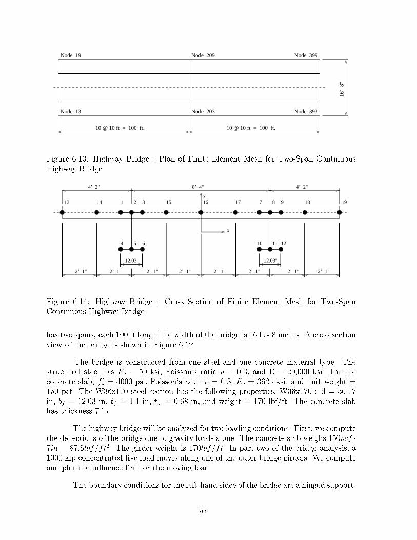
16’

8"

10 @ 10 ft = 100 ft. 10 @ 10 ft = 100 ft.

Node 13 Node 203

Node 19 Node 209 Node 399

Node 393

Figure 6.13: Highway Bridge : Plan of Finite Element Mesh for Two-Span ContinuousHighway Bridge4’ 2"8’ 4"4’ 2"

12.03" 12.03"

2’ 1" 2’ 1" 2’ 1" 2’ 1" 2’ 1" 2’ 1" 2’ 1" 2’ 1"

x

y1 2 3

5 10 11 12

13 14 15 16 17 18987 19

4 6

Figure 6.14: Highway Bridge : Cross Section of Finite Element Mesh for Two-SpanContinuous Highway Bridgehas two spans, each 100 ft long. The width of the bridge is 16 ft - 8 inches. A cross sectionview of the bridge is shown in Figure 6.12.The bridge is constructed from one steel and one concrete material type. Thestructural steel has Fy = 50 ksi, Poisson's ratio v = 0.3, and E = 29,000 ksi. For theconcrete slab, f 0c = 4000 psi, Poisson's ratio v = 0.3, Ec = 3625 ksi, and unit weight =150 pcf. The W36x170 steel section has the following properties; W36x170 : d = 36.17in, bf = 12.03 in, tf = 1.1 in, tw = 0.68 in, and weight = 170 lbf/ft. The concrete slabhas thickness 7 in.The highway bridge will be analyzed for two loading conditions. First, we computethe de ections of the bridge due to gravity loads alone. The concrete slab weighs 150pcf �7in = 87:5lbf=ft2. The girder weight is 170lbf=ft. In part two of the bridge analysis, a1000 kip concentrated live load moves along one of the outer bridge girders. We computeand plot the in uence line for the moving load.The boundary conditions for the left-hand sidee of the bridge are a hinged support.157

The right-hand side of the bridge is supported on a roller. The �nite element model has399 nodes and 440 shell elements. After the boundary conditions are applied, the modelhas 2374 d.o.f. The bridge is subject to a 1000 kip concentrated moving live load.Input File : The following input �le de�nes the bridge geometry, boundary conditions,�nite element, section and material types, and the external loads due to the dead weightof the bridge. START OF INPUT FILE/** =====================================================================* Analysis of Two Span Continuous Composite Beam (100-100ft) assuming* neutral axis of concrete deck coincide with top girder flange** Written By: Wane-Jang Lin December, 1994* =====================================================================*//* [a] : Setup problem specific parameters */print "*** DEFINE PROBLEM SPECIFIC PARAMETERS \n\n";NDimension = 3;NDofPerNode = 6;MaxNodesPerElement = 4;StartMesh();print "*** GENERATE GRID OF NODES FOR FE MODEL \n\n";girder = 2;span = 100 ft;spacing = 8 ft + 4 in;slab = 7 in;height = 36.17 in - 1.1 in;flange = 12.03 in;div_L = 10;div_S = 4;delta_L = span/div_L;delta_S = spacing/div_S;delta_f = flange/2;delta_h = height/2;section_no = 2*div_L + 1;nodes_per_girder = 6;nodes_per_section = nodes_per_girder*girder + (2*div_S+1) - girder;node = 0;x = 0 in;for(i=1 ; i<=section_no ; i=i+1 ) {x = delta_L*(i-1); 158

for( j=1 ; j<=girder ; j=j+1 ) {y = -spacing/2 + spacing*(j-1);AddNode( node+1, [ x, (y-delta_f), delta_h ] );AddNode( node+2, [ x, y , delta_h ] );AddNode( node+3, [ x, (y+delta_f), delta_h ] );AddNode( node+4, [ x, (y-delta_f), -delta_h ] );AddNode( node+5, [ x, y , -delta_h ] );AddNode( node+6, [ x, (y+delta_f), -delta_h ] );node = node + nodes_per_girder;}yy = spacing/2;for( j=1 ; j<=(2*div_S+1) ; j=j+1 ) {y = -spacing + delta_S*(j-1);if( (y!=yy) && (y!=-yy) ) {node = node + 1;AddNode( node, [ x, y, delta_h ] );}}}print "*** ATTACH ELEMENTS TO GRID OF NODES \n\n";elmtno = 0;a = 0;b = 0 + nodes_per_section;for( i=1 ; i<section_no ; i=i+1 ) {for( j=1 ; j<=girder ; j=j+1 ) {AddElmt( elmtno+1, [ a+1, b+1, b+2, a+2 ],"girder_flange_attr" );AddElmt( elmtno+2, [ a+2, b+2, b+3, a+3 ],"girder_flange_attr" );AddElmt( elmtno+3, [ a+2, b+2, b+5, a+5 ],"girder_web_attr" );AddElmt( elmtno+4, [ a+4, b+4, b+5, a+5 ],"girder_flange_attr" );AddElmt( elmtno+5, [ a+5, b+5, b+6, a+6 ],"girder_flange_attr" );elmtno = elmtno + nodes_per_girder - 1;a = a + nodes_per_girder;b = b + nodes_per_girder;}a = a + 1;b = b + 1;for( j=1 ; j<=girder ; j=j+1 ) {AddElmt( elmtno+1, [ a, b, b+1, a+1 ], "deck_attr" );c = b - (girder+1-j)*nodes_per_girder - 3*(j-1);d = a - (girder+1-j)*nodes_per_girder - 3*(j-1);AddElmt( elmtno+2, [ a+1, b+1, c, d ], "deck_attr" );a = d;b = c;AddElmt( elmtno+3, [ a, b, b+1, a+1 ], "deck_attr" );AddElmt( elmtno+4, [ a+1, b+1, b+2, a+2 ], "deck_attr" );a = a + 2;b = b + 2;c = c + (girder+1-j)*nodes_per_girder + (3*j-2) + 1;d = d + (girder+1-j)*nodes_per_girder + (3*j-2) + 1;AddElmt( elmtno+5, [ a, b, c, d ], "deck_attr" );159

AddElmt( elmtno+6, [ d, c, c+1, d+1 ], "deck_attr" );elmtno = elmtno + 6;a = d + 1;b = c + 1;}}print "*** DEFINE ELEMENT, SECTION AND MATERIAL PROPERTIES \n\n";ElementAttr("girder_flange_attr") { type = "SHELL_4NQ";section = "girder_flange";material = "STEEL3";}ElementAttr("girder_web_attr") { type = "SHELL_4NQ";section = "girder_web";material = "STEEL3";}ElementAttr("deck_attr") { type = "SHELL_4NQ";section = "deck";material = "concrete";}SectionAttr("girder_flange") { thickness = 1.100 in; }SectionAttr("girder_web") { thickness = 0.680 in; }SectionAttr("deck") { thickness = 7 in; }MaterialAttr("concrete") { poisson = 0.3;yield = 0.85*(4000 psi);E = (29000 ksi)/8;}print "*** SET UP BOUNDARY CONDITIONS \n\n";bc_hs = [ 1, 1, 1, 1, 0, 0 ]; /* hinged support */bc_rs = [ 0, 1, 1, 1, 0, 0 ]; /* roller support */for( i=1 ; i<=girder ; i=i+1 ) {node = nodes_per_girder*(i-1) + 5;FixNode(node, bc_hs);node = node + div_L*nodes_per_section;FixNode(node, bc_rs);node = node + div_L*nodes_per_section;FixNode(node, bc_rs);}/* [b] : Apply Point Nodal Loads */print "*** SET UP LOADS \n\n";slab_load = (150 lbf/ft^3)*slab;girder_weight = 170 lbf/ft;Fx = 0 lbf; Fy = 0 lbf; 160

Mx = 0 lbf*in; My = 0 lbf*in; Mz = 0 lbf*in;/* [b.1] : load for corner nodes of deck */Fz = -slab_load*delta_L/2*delta_S/2;nodal_load = [Fx, Fy, Fz, Mx, My, Mz];node = nodes_per_girder*girder + 1;NodeLoad(node, nodal_load);node = node + nodes_per_section*(section_no-1);NodeLoad(node, nodal_load);node = node + 2*div_S - girder;NodeLoad(node, nodal_load);node = node - nodes_per_section*(section_no-1);NodeLoad(node, nodal_load);/* [b.2] load for edge nodes along x-direction */Fz = -slab_load*delta_L*delta_S/2;nodal_load = [Fx, Fy, Fz, Mx, My, Mz];node = nodes_per_section + nodes_per_girder*girder + 1;for( i=2 ; i<section_no ; i=i+1 ) {NodeLoad(node, nodal_load);NodeLoad((node+2*div_S-girder), nodal_load);node = node + nodes_per_section;}/* [b.3] load for edge nodes along y-direction *//* node 16 */Fz = -slab_load*delta_L/2*delta_S;nodal_load = [Fx, Fy, Fz, Mx, My, Mz];node = nodes_per_girder*girder + div_S;NodeLoad(node, nodal_load);node = node + nodes_per_section*(section_no-1);NodeLoad(node, nodal_load);/* node 14, 15, 17, 18 */Fz = -slab_load*delta_L/2*(delta_S-delta_f/2);nodal_load = [Fx, Fy, Fz, Mx, My, Mz];node = nodes_per_girder*girder + 1;for( i=1 ; i<=2 ; i=i+1 ) {NodeLoad(node+1, nodal_load);NodeLoad(node+2, nodal_load);NodeLoad(node+4, nodal_load);NodeLoad(node+5, nodal_load);node = node + nodes_per_section*(section_no-1);}/* node 1, 3, 7, 9 */Fz = -slab_load*delta_L/2*delta_S/2;nodal_load = [Fx, Fy, Fz, Mx, My, Mz];node = 0;for( i=1 ; i<=2 ; i=i+1 ) {NodeLoad(node+1, nodal_load); 161

NodeLoad(node+3, nodal_load);NodeLoad(node+7, nodal_load);NodeLoad(node+9, nodal_load);node = node + nodes_per_section*(section_no-1);}/* node 2, 8 */Fz = -slab_load*delta_L/2*delta_f;nodal_load = [Fx, Fy, Fz, Mx, My, Mz];node = 0;for( i=1 ; i<=2 ; i=i+1 ) {NodeLoad(node+2, nodal_load);NodeLoad(node+8, nodal_load);node = node + nodes_per_section*(section_no-1);}/* [b.4] load for middle nodes *//* node 35... */Fz = -slab_load*delta_L*delta_S;nodal_load = [Fx, Fy, Fz, Mx, My, Mz];node = nodes_per_girder*girder + div_S;for( i=2 ; i<section_no ; i=i+1 ) {node = node + nodes_per_section;NodeLoad(node, nodal_load);}/* node 33, 34, 36, 37... */Fz = -slab_load*delta_L*(delta_S-delta_f/2);nodal_load = [Fx, Fy, Fz, Mx, My, Mz];node = nodes_per_girder*girder + 1;for( i=2 ; i<section_no ; i=i+1 ) {node = node + nodes_per_section;NodeLoad(node+1, nodal_load);NodeLoad(node+2, nodal_load);NodeLoad(node+4, nodal_load);NodeLoad(node+5, nodal_load);}/* node 20, 22, 26, 28... */Fz = -slab_load*delta_L*delta_S/2;nodal_load = [Fx, Fy, Fz, Mx, My, Mz];node = 0;for( i=2 ; i<section_no ; i=i+1 ) {node = node + nodes_per_section;NodeLoad(node+1, nodal_load);NodeLoad(node+3, nodal_load);NodeLoad(node+7, nodal_load);NodeLoad(node+9, nodal_load);}/* node 21, 27... */Fz = -slab_load*delta_L*delta_f;nodal_load = [Fx, Fy, Fz, Mx, My, Mz];162

node = 0;for( i=2 ; i<section_no ; i=i+1 ) {node = node + nodes_per_section;NodeLoad(node+2, nodal_load);NodeLoad(node+8, nodal_load);}/* [b.5] load for girder weight *//* end node 2, 8 */Fz = -girder_weight*delta_L/2;nodal_load = [Fx, Fy, Fz, Mx, My, Mz];node = 0;for( i=1 ; i<=2 ; i=i+1 ) {NodeLoad(node+2, nodal_load);NodeLoad(node+8, nodal_load);node = node + nodes_per_section*(section_no-1);}/* middle node 21, 27... */Fz = -girder_weight*delta_L;nodal_load = [Fx, Fy, Fz, Mx, My, Mz];node = 0;for( i=2 ; i<section_no ; i=i+1 ) {node = node + nodes_per_section;NodeLoad(node+2, nodal_load);NodeLoad(node+8, nodal_load);}/* [c] : Compile and Print Finite Element Mesh */EndMesh();PrintMesh();/* [d] : Compute Stiffness Matrix and External Load Vector */print "\n";print "*** COMPUTE AND PRINT STIFFNESS AND EXTERNAL LOAD MATRICES \n\n";SetUnitsType("US");eload = ExternalLoad();stiff = Stiff();/* [e] : Compute and print static displacements */print "\n*** STATIC ANALYSIS PROBLEM \n\n";displ = Solve( stiff, eload);PrintDispl(displ);PrintStress(displ);quit; 163

Abbreviated Output File : Several thousand lines of output are generated by AL-ADDIN and the abovementioned input �le de�ned. Hence, we present an abbreviatedsummary of the output together with contour and three-dimensional views of the bridgedeck de ections. START OF ABBREVIATED OUTPUT FILE===========================================================================Title : DESCRIPTION OF FINITE ELEMENT MESH===========================================================================Problem_Type: Static Analysis=======================Profile of Problem Size=======================Dimension of Problem = 3Number Nodes = 399Degrees of Freedom per node = 6Max No Nodes Per Element = 4Number Elements = 440Number Element Attributes = 3Number Loaded Nodes = 315Number Loaded Elements = 0-----------------------------------------------------------------------------------Node# X_coord Y_coord Z_coord Dx Dy Dz Rx Ry Rz-----------------------------------------------------------------------------------1 0.000e+00 ft -4.667e+00 ft 1.753e+01 in 1 2 3 4 5 62 0.000e+00 ft -4.166e+00 ft 1.753e+01 in 7 8 9 10 11 123 0.000e+00 ft -3.665e+00 ft 1.753e+01 in 13 14 15 16 17 184 0.000e+00 ft -4.667e+00 ft -1.753e+01 in 19 20 21 22 23 24....... details of nodal coordinates deleted .......398 2.000e+02 ft 6.250e+00 ft 1.753e+01 in 2363 2364 2365 2366 2367 2368399 2.000e+02 ft 8.333e+00 ft 1.753e+01 in 2369 2370 2371 2372 2373 2374----------------------------------------------------------------------------------Element# Type node[1] node[2] node[3] node[4] Element_Attr_Name----------------------------------------------------------------------------------1 SHELL_4NQ 1 20 21 2 girder_flange_attr2 SHELL_4NQ 2 21 22 3 girder_flange_attr3 SHELL_4NQ 2 21 24 5 girder_web_attr4 SHELL_4NQ 4 23 24 5 girder_flange_attr164

....... details of shell finite elements removed .......437 SHELL_4NQ 368 387 388 369 deck_attr438 SHELL_4NQ 369 388 389 370 deck_attr439 SHELL_4NQ 370 389 398 379 deck_attr440 SHELL_4NQ 379 398 399 380 deck_attr---------------------Element Attribute Data :---------------------ELEMENT_ATTR No. 1 : name = "girder_flange_attr": section = "girder_flange": material = "STEEL3": type = SHELL_4NQ: dof-mapping : gdof[0] = 1 : gdof[1] = 2 : gdof[2] = 3gdof[3] = 4 : gdof[4] = 5 : gdof[5] = 6: Young's Modulus = E = 2.900e+04 ksi: Yielding Stress = fy = 5.000e+01 ksi: Poisson's ratio = nu = 3.000e-01: Density = 0.000e+00 (null): Inertia Izz = 0.000e+00 (null): Area = 0.000e+00 (null)ELEMENT_ATTR No. 2 : name = "girder_web_attr": section = "girder_flange": material = "STEEL3": type = SHELL_4NQ: dof-mapping : gdof[0] = 1 : gdof[1] = 2 : gdof[2] = 3gdof[3] = 4 : gdof[4] = 5 : gdof[5] = 6: Young's Modulus = E = 2.900e+04 ksi: Yielding Stress = fy = 5.000e+01 ksi: Poisson's ratio = nu = 3.000e-01: Density = 0.000e+00 (null): Inertia Izz = 0.000e+00 (null): Area = 0.000e+00 (null)ELEMENT_ATTR No. 3 : name = "deck_attr": section = "deck": material = "concrete": type = SHELL_4NQ: dof-mapping : gdof[0] = 1 : gdof[1] = 2 : gdof[2] = 3gdof[3] = 4 : gdof[4] = 5 : gdof[5] = 6: Young's Modulus = E = 3.625e+03 ksi: Yielding Stress = fy = 3.400e+03 psi: Poisson's ratio = nu = 3.000e-01: Density = 0.000e+00 (null): Inertia Izz = 0.000e+00 (null): Area = 0.000e+00 (null)EXTERNAL NODAL LOADINGS-------------------------------------------------------------------------------165

Node# Fx (lbf) Fy (lbf) Fz (lbf) Mx (lbf.in) My (lbf.in) Mz (lbf.in)-------------------------------------------------------------------------------13 0.000 0.000 -455.729 0.000 0.000 0.000393 0.000 0.000 -455.729 0.000 0.000 0.000399 0.000 0.000 -455.729 0.000 0.000 0.00019 0.000 0.000 -455.729 0.000 0.000 0.00032 0.000 0.000 -911.458 0.000 0.000 0.00038 0.000 0.000 -911.458 0.000 0.000 0.000..... details of nodal loads removed ....344 0.000 0.000 -1700.000 0.000 0.000 0.000350 0.000 0.000 -1700.000 0.000 0.000 0.000363 0.000 0.000 -1700.000 0.000 0.000 0.000369 0.000 0.000 -1700.000 0.000 0.000 0.000============= End of Finite Element Mesh Description ==============*** COMPUTE AND PRINT STIFFNESS AND EXTERNAL LOAD MATRICES*** STATIC ANALYSIS PROBLEM------------------------------------------------------------------------------Node DisplacementNo displ-x displ-y displ-z rot-x------------------------------------------------------------------------------units in in in rad1 1.33978e-01 -1.89314e-05 -1.80219e-03 2.02410e-042 1.34131e-01 -2.29040e-05 -7.12851e-04 1.58344e-043 1.34036e-01 -2.64397e-05 1.11846e-04 1.17222e-044 4.80519e-04 7.93065e-05 -3.01849e-06 7.53268e-075 0.00000e+00 0.00000e+00 0.00000e+00 0.00000e+0013 1.32863e-01 -3.34551e-05 -1.44068e-02 3.23153e-04....... details of nodal displacements removed ......395 7.72668e-02 -5.87620e-05 1.43256e-03 3.45080e-05396 7.74839e-02 -9.59758e-13 1.76084e-03 5.23559e-16397 7.72668e-02 5.87620e-05 1.43256e-03 -3.45080e-05398 7.74887e-02 -1.71932e-05 -6.61126e-03 -2.90572e-04399 7.79492e-02 3.34551e-05 -1.44068e-02 -3.23153e-04Figures 6.15 and 6.16 are contour and three-dimensional views of the bridge deck de- ections, respectively. (the vertical axis of the de ection of Figure 6.16 has the units ofinches). The bridge de ections are due to dead loads alone, and since the bridge geome-try and section properties are symmetric, we expect that the de ections will also exhibitsymmetry. They do.166

1 2 3 4 5 6 7 8 9

2

4

6

8

10

12

14

16

18

20

Figure 6.15: Highway Bridge : Contour Plot of Bridge Deck De ections

02

46

810

0

5

10

15

20

25−1.5

−1

−0.5

0

0.5

Bridge Deck Displacements

Figure 6.16: Three-Dimensional Mesh of Bridge Deck De ections167

Moving Point Load Input File : In Part 2 of our analysis, the latter sections of theinput �le are extended so that response evelopes are computed for a point load movingalong the bridge.

FRAMING PLAN

FRONT ELEVATION

100 ft. 100 ft.

4’ 2

"4’

2"

16’

8"

LOAD DIRECTION

10 LOAD INCREMENTS @ 10 FT 10 LOAD INCREMENTS @ 10 FT

LOAD DIRECTION

Figure 6.17: Plan and Front Elevation of Two-Span Continuous Highway Bridge withMoving Live LoadFigure 6.17 shows plan and elevation views of the bridge and moving point load. Across sectional view of the bridge and the moving point load is shown in Figure 6.18.Abbreviated details of the input �le are as follows:START OF INPUT FILE/** =====================================================================* Analysis of Two Span Continuous Composite Beam (100-100ft), analysis* assuming neutral axis of concrete deck coincide with top girder flange* Moving load along one girder** Written By: Wane-Jang Lin December, 1994* =====================================================================*//* [a] : Setup problem specific parameters */168

W36x170 W36x170

4’ 2" 4’ 2"8’ 4"

1000 KIPS [ MOVING LOAD ]

CROSS SECTION OF HIGHWAY BRIDGE WITH MOVING LIVE LOADFigure 6.18: Cross Section of Two-Span Continuous Highway Bridge with Moving LiveLoadNDimension = 3;NDofPerNode = 6;MaxNodesPerElement = 4;StartMesh();print "*** GENERATE GRID OF NODES FOR FE MODEL \n\n";..... details are the same as in static analysis datafile ....print "*** ATTACH ELEMENTS TO GRID OF NODES \n\n";..... details are the same as in static analysis datafile ....print "*** DEFINE ELEMENT, SECTION AND MATERIAL PROPERTIES \n\n";..... details are the same as in static analysis datafile ....print "*** SET UP BOUNDARY CONDITIONS \n\n";..... details are the same as in static analysis datafile ..../* [b] : Compile and Print Finite Element Mesh */EndMesh();PrintMesh();/* [c] : Compute Stiffness Matrix */SetUnitsType("US");stiff = Stiff();/* [d] : Compute Influence Lines for Moving Live Loads */print "\n*** STATIC ANALYSIS PROBLEM \n\n";Fx = 0 lbf; Fy = 0 lbf; Fz = -1000.0 kips;169

Mx = 0 lbf*in; My = 0 lbf*in; Mz = 0 lbf*in;nodeno1 = 97;nodeno2 = 103;step = div_L*2+1;print "node no 1 =",nodeno1,"\n";print "node no 2 =",nodeno2,"\n";print "Fz =",Fz,"\n";print "step =",step,"\n";influ_line1 = Zero([ step , 1 ]); /* array for influence line 1 */influ_line2 = Zero([ step , 1 ]); /* array for influence line 2 */load_node = 2;lu = Decompose (stiff);for( i=1 ; i<=step ; i=i+1 ) {NodeLoad( load_node, [Fx,Fy,Fz,Mx,My,Mz] );eload = ExternalLoad();displ = LUDecomposition( stiff, eload );node_displ_1 = GetDispl( [nodeno1], displ );node_displ_2 = GetDispl( [nodeno2], displ );influ_line1[i][1] = node_displ_1[1][3];influ_line2[i][1] = node_displ_2[1][3];NodeLoad( load_node, [-Fx,-Fy,-Fz,-Mx,-My,-Mz] );load_node = load_node + nodes_per_section;}PrintMatrix(influ_line1);PrintMatrix(influ_line2);quit;Figure 6.19 shows the in uence line of vertical displacement in the middle of one span(i.e. at node no 97) for the �rst girder subjected to 1000 kips moving live load. Similarly,Figure 6.20 shows the in uence line of displacement in the middle of one span (i.e. nodeno 2 = 103) due to the 1000 kips moving live load.The moving load analysis is one situation where a family of linear equations issolved with multiple right-hand sides. With this in mind, notice how we have calledthe function Decompose() once to decompose stiff into a product of upper and lowertriangular matrices, and then called LUDecomposition() to compute the forward andbackward substitution for each analysis. This strategy of equation solving reduces theoverall solution time by approximately 70%.170

0 20 40 60 80 100 120 140 160 180 200−30

−25

−20

−15

−10

−5

0

5

10

First girder coordinate (ft)

Ver

tical

def

lect

ion

(in)

Figure 6.19: In uence line of displacement in the middle of one span for the �rst girdersubjected to 1000 kips moving live load

0 20 40 60 80 100 120 140 160 180 200−12

−10

−8

−6

−4

−2

0

2

4

6

Middle girder coordinate (ft)

Ver

tical

def

lect

ion

(in)

Figure 6.20: In uence line of displacement in the middle of one span for the second girder171

6.2 Time-History Analyses6.2.1 Modal Analysis of Five Story Steel FrameDescription of Problems : In this section we compute the linear time-history responseof the steel frame structure described in Section 6.1.1. to dead and live gravity loads, plusa 1979 El Centro Earthquake ground motion scaled to moderate intensity.

50

ft

55 ft

4

5

3

2

1

Full Fixity

FLOOR 1

FLOOR 2

FLOOR 3

FLOOR 4

ROOF

ELEVATION VIEW OF STEEL FRAME SIMPLIFIED MODEL

Xg ( t )Xg ( t )Figure 6.21: Elevation View and Simpli�ed Model of Moment Resistant Frame subject toScaled 1979 El Centro EarthquakeThe left-hand side of Figure 6.21 is a simpli�ed elevation view of the frame also shown inFigure 6.1. Unlike the analysis conducted in Section 6.1.1., we will assume that all nodalrotations and vertical de ections of the frame are fully restrained, and that the horizontalde ections across each oor may be lumped into a single degree of freedom. Together theseassumptions imply that each oor will move as a rigid body in the horizontal direction,and that the global frame behavior may be described with only �ve degrees of freedom.The right-hand side of Figure 6.21 shows the simpli�ed model that will be used in theearthquake time-history analysis { the shaded �lled boxes represent the lumped massesat each oor level, and the global degrees of freedom begin at the �rst oor level andincrease to the roof.Figure 6.22 shows details of a 10 segment accelerograph extracted from the 1979 ElCentro Earthquake ground motion. The peak ground acceleration is 86.63 cm/sec/sec.The ground motion will be scaled so that the peak ground acceleration is 0.15 g.Input File : The following input �le is based on the input �le presented in Section 6.1.1,172

0 1 2 3 4 5 6 7 8 9 10−1

−0.8

−0.6

−0.4

−0.2

0

0.2

0.4

0.6

0.8

Time ( seconds )

Gro

und

Acc

eler

atio

n (m

/sec

/sec

)

Figure 6.22: Ground Acceleration for 1979 El Centro Earthquakewith appropriate extensions for the earthquake analysis, and generation of time-historyresponse quantities for post-analysis plotting.START OF INPUT FILE/** ============================================================* Modal Analysis of Five Story Steel Moment Frame subject to* El Centro ground motion.** Written By: Mark Austin July, 1995* ============================================================*//* [a] : Setup problem specific parameters */NDimension = 2;NDofPerNode = 3;MaxNodesPerElement = 2;StartMesh();/* [b] : Generate two-dimensional grid of nodes */..... same as for five story building ..../* [c] : Attach column elements to nodes */173

..... same as for five story building ..../* [d] : Attach beam elements to nodes */..... same as for five story building ..../* [e] : Define section and material properties */ElementAttr("mrf_element") { type = "FRAME_2D";section = "mrfsection";material = "mrfmaterial";}SectionAttr("mrfsection") { Izz = 1541.9 in^4;Iyy = 486.3 in^4;depth = 12.0 in;width = 12.0 in;area = 47.4 in^2;}MaterialAttr("mrfmaterial") { density = 7850 kg/m^3;poisson = 0.27;yield = 275000 MPa;E = 200000 MPa;}/* [f] : Apply full-fixity to columns at foundation level */for(nodeno = 1; nodeno <= 4; nodeno = nodeno + 1) {FixNode( nodeno, [ 1, 1, 1 ]);}for(nodeno = 5; nodeno <= 24; nodeno = nodeno + 1) {FixNode( nodeno, [ 0, 1, 1 ]);}LinkNode([ 5, 6, 7, 8 ], [ 1, 0, 0] );LinkNode([ 9, 10, 11, 12 ], [ 1, 0, 0] );LinkNode([ 13, 14, 15, 16 ], [ 1, 0, 0] );LinkNode([ 17, 18, 19, 20 ], [ 1, 0, 0] );LinkNode([ 21, 22, 23, 24 ], [ 1, 0, 0] );/* [g] : Compile and Print Finite Element Mesh */EndMesh();PrintMesh();/* [h] : Compute "stiffness" matrix; manually assemble "mass" matrices */stiff = Stiff();PrintMatrix(stiff);mass = Zero([5,5]); 174

mass = ColumnUnits ( mass , [N/m] );mass = RowUnits ( mass , [sec^2] );/* [i] : Manually assemble "mass" matrix : assume (dead + live) loads */dead_load = 80 lbf/ft^2;floor_live_load = 40 lbf/ft^2;roof_live_load = 20 lbf/ft^2;frame_spacing = 20 ft;floor_length = 55 ft;tributary_area = frame_spacing * floor_length;for(i = 1; i <= 5; i = i + 1) {if(i <= 4) then {floor_load = tributary_area * (dead_load + floor_live_load);} else {floor_load = tributary_area * (dead_load + roof_live_load);}mass [i][i] = mass[i][i] + floor_load / (32.2 ft/sec^2);}PrintMatrix(mass);/* [j] : Compute and print eigenvalues and eigenvectors */no_eigen = 2;eigen = Eigen(stiff, mass, [ no_eigen ]);eigenvalue = Eigenvalue(eigen);eigenvector = Eigenvector(eigen);for(i = 1; i <= no_eigen; i = i + 1) {print "Mode", i ," : w^2 = ", eigenvalue[i][1];print " : T = ", 2*PI/sqrt(eigenvalue[i][1]) ,"\n";}PrintMatrix(eigenvector);/* [k] : Generalized mass and stiffness matrices */EigenTrans = Trans(eigenvector);Mstar = EigenTrans*mass*eigenvector;Kstar = EigenTrans*stiff*eigenvector;PrintMatrix( Mstar );PrintMatrix( Kstar );/* [m] : Setup Rayleigh Damping for Frame Structure */rdamping = 0.05;W1 = sqrt ( eigenvalue[1][1]);W2 = sqrt ( eigenvalue[2][1]);A0 = 2*rdamping*W1*W2/(W1 + W2); 175

A1 = 2*rdamping/(W1 + W2);print "A0 = ", A0, " A1 = ", A1, "\n";Cstar = A0*Mstar + A1*Kstar;PrintMatrix( Cstar );/* [n] : Define earthquake loadings... */Elcentro = ColumnUnits( [14.56; 13.77; 6.13; 3.73; 1.32; -6.81; -16.22; -22.41;...... details of earthquake removed .....-10.05; -12.35; -15.72; 0.00 ], [cm/sec/sec] );ground_motion_scale_factor = 0.15*981.0/86.63;PrintMatrix( Elcentro );/* [o] : Initialize system displacement, velocity, and load vectors */displ = ColumnUnits( Matrix([5,1]), [m] );vel = ColumnUnits( Matrix([5,1]), [m/sec]);eload = ColumnUnits( Matrix([5,1]), [kN]);r = One([5,1]);/* [p] : Initialize modal displacement, velocity, and acc'n vectors */Mdispl = ColumnUnits( Matrix([ no_eigen,1 ]), [m] );Mvel = ColumnUnits( Matrix([ no_eigen,1 ]), [m/sec]);Maccel = ColumnUnits( Matrix([ no_eigen,1 ]), [m/sec/sec]);/** [q] : Allocate Matrix to store five response parameters --* Col 1 = time (sec);* Col 2 = 1st mode displacement (cm);* Col 3 = 2nd mode displacement (cm);* Col 4 = 1st + 2nd mode displacement (cm);* Col 5 = Total energy (Joules)*/dt = 0.02 sec;nsteps = 600;beta = 0.25;gamma = 0.5;response = ColumnUnits( Matrix([nsteps+1,5]), [sec], [1]);response = ColumnUnits( response, [cm], [2]);response = ColumnUnits( response, [cm], [3]);response = ColumnUnits( response, [cm], [4]);response = ColumnUnits( response, [Jou], [5]);/* [r] : Compute (and compute LU decomposition) effective mass */176

MASS = Mstar + rdamping*dt*Cstar + Kstar*beta*dt*dt;lu = Decompose(Copy(MASS));/* [s] : Mode-Displacement Solution for Response of Undamped MDOF System */MassTemp = -mass*r;for(i = 1; i <= nsteps; i = i + 1) {print "*** Start Step ",i,"\n";if(i == 2) {SetUnitsOff;}/* [s.1] : Update external load */if(i <= 500) then {eload = MassTemp*Elcentro[i][1]*ground_motion_scale_factor;} else {eload = MassTemp*(0)*ground_motion_scale_factor;}Pstar = EigenTrans*eload;R = Pstar - Kstar*(Mdispl + Mvel*dt + Maccel*(dt*dt/2.0)*(1-2*beta)) -Cstar*(Mvel + Maccel*dt*(1-gamma));/* [s.2] : Compute new acceleration, velocity and displacement */Maccel_new = Substitution(lu,R);Mvel_new = Mvel + dt*(Maccel*(1.0-gamma) + gamma*Maccel_new);Mdispl_new = Mdispl + dt*Mvel + ((1 - 2*beta)*Maccel +2*beta*Maccel_new)*dt*dt/2;/* [s.3] : Update and print new response */Maccel = Maccel_new;Mvel = Mvel_new;Mdispl = Mdispl_new;/* [s.4] : Combine Modes */displ = eigenvector*Mdispl;vel = eigenvector*Mvel;/* [s.5] : Compute Total System Energy */a1 = Trans(vel);a2 = Trans(displ);e1 = a1*mass*vel;e2 = a2*stiff*displ;energy = 0.5*(e1 + e2);/* [s.6] : Save components of time-history response */177

response[i+1][1] = i*dt; /* Time */response[i+1][2] = eigenvector[1][1]*Mdispl[1][1]; /* 1st mode displacement */response[i+1][3] = eigenvector[1][2]*Mdispl[2][1]; /* 2nd mode displacement */response[i+1][4] = displ[1][1]; /* 1st + 2nd mode displacement */response[i+1][5] = energy[1][1]; /* System Energy */}/* [t] : Print response matrix and quit */SetUnitsOn;PrintMatrix(response);quit;Points to note are:[1] Notice that we have used the �nite element routines to compute the sti�ness matrix,but have manually assembled the mass matrix. It is assumed that when the earth-quake occurs, the frame loads will equal the dead loading plus the full live loading.The tributary area equals the frame spacing (20 ft) times the frame width (55 ft).[2] The global mass and sti�ness matrices are (5�5) matrices. The time-history analysisis simpli�ed by computing the Newmark integration on the �rst and second modesof the frame alone. The generalized mass and sti�ness matrices are as described inSection 4.3.[3] The damping matrix is taken as a linear combination of the generalized mass andsti�ness matrices, namely: C� = ao �M� + a1 �K�: (6.3)Let wm and �m be the circular natural frequency and ratio of critical damping inthe mode m, and wn and �n be the circular natural frequency and ratio of criticaldamping in the mode n. It can be shown that the coe�cients a1 and a2 are givenby: " a1a2 # = 2 � wm � wnw2n � w2m � " wn �wm�1=wn 1=wm # � " �m�n # (6.4)For this analysis we will letm = 1 and n = 2, and assume that the critical ratio ofdamping is the same in both modes. The input �le variable rdamping represents theratio of critical damping in the �rst and second modes. Analyses will be conductedfor rdamping = 0.0, and rdamping = 0.05.[4] The time-history analysis is based on the Newmark equations given in Section 4.2,and the modal analysis equations speci�ed in Section 4.3. At each step the analysiswe compute solutions to the equation of equilibrium178

�TM� �Y (t) +�TC� _Y (t) +�TK�Y (t) = �TP (t) = ��TMr �Xg(t): (6.5)Here �, M, C, and K are as previously de�ned. r is a (5 � 1) that describes themovement in each of the frame degrees of freedom due to a unit ground displacement{ in this case, r = (5� 1) vector of ones. �Xg(t) is the ground acceleration at time t.[5] The response is computed for 600 steps of time-step 0.02 seconds (i.e. 12 seconds).The �rst loop of analysis is conducted with the units checking turned on { thereafter,the units are switched o�. Constant acceleration across each time-step is achievedby setting the Newmark parameters � = 0:25 and = 0:5 { see Section 4.2 for adetailed discussion on the Newmark method.[6] At the end of each time-step we compute the sum of kinetic plus potential energy forthe frame's �rst two modes. Theoretical considerations indicate that when � = 0:25and = 0:5, the total energy of the undamped system will be conserved after theearthquake motion has stopped (i.e. the last 2 seconds of the computed response).[7] We have allocated a 600 by 5 response matrix to stored selected components of thetime-history response. See the input �le for a description of the contents in eachcolumn.Abbreviated Output File : The following output �le is a summary of the outputgenerated for the simulation case rdamping = 0.0.START OF ABBREVIATED OUTPUT FILE==========================================Title : DESCRIPTION OF FINITE ELEMENT MESH=================================================================Profile of Problem Size=======================Dimension of Problem = 2Number Nodes = 24Degrees of Freedom per node = 3Max No Nodes Per Element = 2Number Elements = 35Number Element Attributes = 1Number Loaded Nodes = 0Number Loaded Elements = 0------------------------------------------------------------Node# X_coord Y_coord Tx Ty Rz------------------------------------------------------------179

1 0.0000e+00 ft 0.0000e+00 ft -1 -2 -32 2.0000e+01 ft 0.0000e+00 ft -4 -5 -63 3.5000e+01 ft 0.0000e+00 ft -7 -8 -94 5.5000e+01 ft 0.0000e+00 ft -10 -11 -12..... details of nodal coordinates removed .....24 5.5000e+01 ft 5.0000e+01 ft 5 -51 -52------------------------------------------------------------------Element# Type node[1] node[2] Element_Attr_Name------------------------------------------------------------------1 FRAME_2D 1 5 mrf_element2 FRAME_2D 5 9 mrf_element..... details of frame elements removed .....34 FRAME_2D 22 23 mrf_element35 FRAME_2D 23 24 mrf_element------------------------Element Attribute Data :------------------------ELEMENT_ATTR No. 1 : name = "mrf_element": section = "mrfsection": material = "mrfmaterial": type = FRAME_2D: gdof [0] = 1 : gdof[1] = 2 : gdof[2] = 3: Young's Modulus = E = 2.000e+05 MPa: Yielding Stress = fy = 2.750e+05 MPa: Poisson's ratio = nu = 2.700e-01: Density = 7.850e+03 kg/m^3: Inertia Izz = 1.542e+03 in^4: Area = 4.740e+01 in^2============= End of Finite Element Mesh Description ==============SKYLINE MATRIX : "stiff"row/col 1 2 3 4 5units N/m N/m N/m N/m N/m1 4.35158e+08 -2.17579e+08 0.00000e+00 0.00000e+00 0.00000e+002 -2.17579e+08 4.35158e+08 -2.17579e+08 0.00000e+00 0.00000e+003 0.00000e+00 -2.17579e+08 4.35158e+08 -2.17579e+08 0.00000e+004 0.00000e+00 0.00000e+00 -2.17579e+08 4.35158e+08 -2.17579e+085 0.00000e+00 0.00000e+00 0.00000e+00 -2.17579e+08 2.17579e+08MATRIX : "mass"row/col 1 2 3 4 5units N/m N/m N/m N/m N/m180

1 sec^2 5.98259e+04 0.00000e+00 0.00000e+00 0.00000e+00 0.00000e+002 sec^2 0.00000e+00 5.98259e+04 0.00000e+00 0.00000e+00 0.00000e+003 sec^2 0.00000e+00 0.00000e+00 5.98259e+04 0.00000e+00 0.00000e+004 sec^2 0.00000e+00 0.00000e+00 0.00000e+00 5.98259e+04 0.00000e+005 sec^2 0.00000e+00 0.00000e+00 0.00000e+00 0.00000e+00 4.98550e+04*** SUBSPACE ITERATION CONVERGED IN 9 ITERATIONSMode 1 : w^2 = 313 1/sec^2 : T = 0.3551 secMode 2 : w^2 = 2648 1/sec^2 : T = 0.1221 secMATRIX : "eigenvector"row/col 1 2units1 2.91629e-01 7.87127e-012 5.58155e-01 1.00000e+003 7.76637e-01 4.84597e-014 9.28270e-01 -3.82551e-015 1.00000e+00 -9.70739e-01MATRIX : "Mstar"row/col 1 2units N/m N/m1 sec^2 1.61217e+05 7.27596e-122 sec^2 7.27596e-12 1.66677e+05MATRIX : "Kstar"row/col 1 2units N/m N/m1 5.04687e+07 2.04891e-082 0.00000e+00 4.41345e+08A0 = 0 1/sec A1 = 0 secMATRIX : "Cstar"row/col 1 2units kg/sec^3 kg/sec^31 sec^2 0.00000e+00 0.00000e+002 sec^2 0.00000e+00 0.00000e+00MATRIX : "response"row/col 1 2 3 4 5units sec cm cm cm Jou1 0.00000e+00 0.00000e+00 0.00000e+00 0.00000e+00 0.00000e+002 2.00000e-02 -5.17642e-04 -3.51330e-04 -8.68972e-04 2.82918e-01...... details of response matrix removed : for details, see the figures.600 1.19800e+01 -4.21771e-02 -2.57188e-02 -6.78958e-02 3.88629e+02601 1.20000e+01 -7.47478e-02 -1.97584e-02 -9.45062e-02 3.88629e+02181

Matrices Mstar and Kstar in the program output correspond to the generalized massand sti�ness matrices, respectively. We expect that the computed eigenvectors will beorthogonal with respect to the mass and sti�ness matrices, and hence, the generalizedmass and sti�ness matrices will be (nearly) diagonal { we see that in practice, someround-o� errors occur.The �rst and second modes of vibration have natural periods 0.3551 sec and0.1221 sec, respectively. When the frame is undamped, coe�cients ao and a1 evaluate tozero, as expected.Figures 6.23 to 6.26 summarize the time-history response of the undamped mo-ment resistant frame. Figure 6.23 is the time history response for mode 1, Figure 6.24 thetime history response for mode 2, and Figure 6.25 the time history response for modes 1and 2 combined. Figure 6.26 plots the kinetic plus potential energy of the frame { youshould notice that once the ground motion has ceased (at t = 10 seconds), the Newmarkmethod conserves energy.Figures 6.27 and 6.27 plot the total time-history response and energy when theframe has 5% damping. After the ground motion has ceased, the roof displacementdecreases steadily to zero. You can easily observe that between t = 10 seconds and t = 12seconds, the roof oscillates through approximately 5.5 cycles. This implies an approximatenatural frequency of 2=5:5 � 0:36 seconds.

182

0 2 4 6 8 10 12−0.6

−0.4

−0.2

0

0.2

0.4

0.6

Time (seconds)

Dis

plac

emen

t (cm

)

Figure 6.23: Modal Analysis : First Mode Displacement of Roof (cm) versus Time (sec)

0 2 4 6 8 10 12−0.1

−0.08

−0.06

−0.04

−0.02

0

0.02

0.04

0.06

0.08

Time (seconds)

Dis

plac

emen

t (cm

)

Figure 6.24: Modal Analysis : Second Mode Displacement of Roof (cm) versus Time (sec)183

0 2 4 6 8 10 12−0.5

−0.4

−0.3

−0.2

−0.1

0

0.1

0.2

0.3

0.4

0.5

Time (seconds)

Dis

plac

emen

t (cm

)

Figure 6.25: Modal Analysis : First + Second Mode Displacement of Roof (cm) versusTime (sec)

0 2 4 6 8 10 120

1000

2000

3000

4000

5000

6000

7000

8000

9000

Time (seconds)

Tot

al E

nerg

y (J

oule

s)

Figure 6.26: Modal Analysis : Total Energy (Joules) versus Time (sec)184

0 2 4 6 8 10 12−0.4

−0.3

−0.2

−0.1

0

0.1

0.2

0.3

0.4

Time (seconds)

Dis

plac

emen

t (cm

)

Figure 6.27: Modal Analysis at 5% damping : First + Second Mode Displacement of Roof(cm) versus Time (sec)

0 2 4 6 8 10 120

500

1000

1500

2000

2500

3000

3500

4000

4500

Time (seconds)

Tot

al E

nerg

y (J

oule

s)

Figure 6.28: Modal Analysis at 5% damping : Total Energy (Joules) versus Time (sec)185

Part IVARCHITECTURE AND DESIGN

186

Chapter 7Data Types : Physical Quantity andMatrix Data Structures7.1 IntroductionBasic engineering quantities such as, length, mass, and force, are de�ned by anumerical value (number itself) plus physical units. The importance of the engineeringunits is well known. Unfortunately, physical units are not a standard part of main-stream�nite element software packages { indeed, most engineering software packages simplyassume that engineering units will be consistent, and leave the details of checking toengineer (in the writers' experience, it is not uncommon for engineers to overlook thisdetail). While this practice of implementation may be satisfactory for computation ofwell established algorithms, it is almost certain to lead to incorrect results when engineersare working on the development of new and innovative computations.ALADDIN deviates from this trend by supporting the basic data type physicalquantity, as well as matrices of physical quantities. Engineers may de�ne units as partof the problem description, and manipulate these quantities via standard arithmetic andmatrix operations. Any set of valid engineering units can be used. For example, mm, cm,m, km, and in, are all valid units of length. In this chapter, we discuss the data structuresused to implement physical quantities, and matrices of physical quantities. Special storagetechniques for large symmetric matrices are also mentioned.7.2 Physical QuantitiesAny physical unit can be decomposed into basic units. The four basic units neededfor engineering analysis are: length unit L; mass unit M; time unit t; and temperatureunit T . Any engineering unit can be obtained with the following combinations:unit = kL�M�t T �:187

where �; �; ; � are exponents, and k is the scale factor. For units of length and mass,[�; �; ; �] = [1; 0; 0; 0] and [�; �; ; �] = [0; 1; 0; 0], respectively. Non-dimensional quan-tities (i.e. numbers, degrees, and radians) are given by the family of zero exponents[�; �; ; �] = [0; 0; 0; 0]. With this basic units in place, we can de�ne the units data struc-ture as: #define SI 100#define US 200#define SI_US 300typedef struct dimensional_exponents {char *units_name; /* units name */double scale_factor; /* scale/conversion factor */double length_expnt; /* exponent for length */double mass_expnt; /* exponent for mass */double time_expnt; /* exponent for time */double temp_expnt; /* exponent for temperature */int units_type; /* US or SI units */} DIMENSIONS;The character string stores the unit name, and scale factor, the scale factor with respectto a basic unit. For example, in US units the basic unit of length is inch. It follows that12 will be the scale factor for one foot. The units type ag allows for the representation ofvarious systems of units (e.g. SI, US, and combined SI US). SI US units are those sharedby both US and SI systems { the two most important examples being time and non-dimensional units. We use variables of data type double to represent exponents, therebyavoiding mathematical di�culties in manipulation of quantities. For example, if x = y0:5,the unit exponents of x, [�x; �x; x; �x] = 0:5� [�y; �y; y; �y]. If the units exponents werede�ned as integers, then x would be incorrectly truncated to [�x; �x; x; �x] = [0; 0; 0; 0].With the units data structure in place, the quantity data structure is simply de�ned astypedef struct engineering_quantity {double value;DIMENSIONS *dimen;} QUANTITY;Notice that physical units alone are the special case of a quantity with numerical value1.0.7.2.1 Relationship between Quantity and UnitsIn engineering applications, there is no need to distinguish between di�erent sys-tems of units during calculation. The main use of units is for clari�cation of probleminput and problem output. ALADDIN stores a physical quantity as an unscaled valuewith respect to a set of reference units, and by default, all quantities are stored internallyin the SI units system. In the SI system, the reference set of units are meter \m" forlength, kilogram \kg" for mass, second \sec" for time and \deg C" for temperature.188

Suppose, for example, that we de�ne the quantity, x = 1 km (one kilometer).Because 1 km = 1000 m, x will be saved internally as value = 1000, In the data structureDIMENSIONS, units name will point to the character string \km". The scale factor for\km" with respect to reference unit \m" is 1000. Now lets see what happens when weprint x. Because the output value = value/scale factor = 1. \print x" will still give \1km".7.2.2 US and SI Units ConversionScale factors are needed to convert units in US to SI, and vice versa. All quantitiesin US units must be converted into SI before they can be used in calculations. Fortunately,for most sets of units, only a single scale factor is needed to convert a quantity from USinto SI and vice versa (e.g. 1 in = 24.5 mm = 25.4E-3 m).The important exception is temperature units. Conversion of temperature units iscomplicated by the nonlinear relationship between systems { that is xoF 6= x�1oF , sincexoF = (5=9)(x� 32)� 1oC. In other words, the value and unit of a temperature quantitycan not be treated separately. We have to know the value of temperature before we canconvert it's units from one to another unit system. ALADDIN handles this problem by�rst installing the \deg F" (unit for oF ) with scale factor = 1 into symbol table. Whenthe value (a number) and the unit are combined into a quantity we convert the deg F intodeg C. When a temperature quantity is printed out, we need to convert it's units to theprefered units. A related complication is units for temperature increment. One degree oftemperature increase is di�erent from one degree temperature. To see how this problemarises, let y = 1oF . If y is a one degree temperature increase, then y = (�+1)oF ��oF =5=9oC, where � is value of previous temperature. If, on the other hand, y is at one degreeFahrenheit temperature, then y = (5=9)(1� 32)oC = �17:22oC. Similar di�culties cropup in the computation of temperature gradient { 10mm=oF can only be considered asa 10 mm extension for one Fahrenheit degree temperature increase, which is 18mm=oC.This cannot be considered as (10mm)=(1oF ), which is (�0:5806mm)=(1oC) (divisions ofthis kind in real engineering computations are meaningless). To avoid these confusions, anew set of units are chosen for temperature increments, they are "DEG F and DEG C"to distinguish from \deg F and deg C". The conversion between DEG F and DEG C isDEG F = 5/9 DEG C. And for simplicity, we will ignore the case of (10mm)=(1oF ).Library Functions for Internal Operations on Units : ALADDIN also providesfunctions for internal operations on units { example functions include copying units,obtaining default units, checking consistency of units, simplifying the units name aftervarious operations, calculating the length of units name, and printing of units. For asummary of functions, see Table 7.1. Note : Some mathematical functions such aslog(x), ln(x) or exp(x), cannot have units in their argument lists. Other mathematicalfunctions, such as sine and cosine, can only have degree or radian in their arguments.189

Functions for Units OperationsFunction Purpose of FunctionSameUnits() Check if two units are of same typeUnitsMult() Multiply two unitsUnitsDiv() Divide two unitsUnitsCopy() Make a copy of a unitUnitsPower() compute a unit raised to a powerUnitsNegate() Negate a unit d = 1/dUnitsPrint() Print name, scalefactor, type and exponents of a unitZeroUnits() Initialize a unitDefaultUnits() Determine pointer on symbol table for a given unit nameUnitsSimplify() Simplify unit name string with simple character stringRadUnitsSimplify() Convert a nondimensional unit into a radian unitUnitsLength() Measure the total length of several units namesConvertTempUnits() Convert temperature units between SI and US systemsUnitsConvert() Convert units between US and SI systems { except fortemperature unitsTable 7.1: Functions for Units Operations

190

7.3 MatricesALADDIN's matrix module has following features:[1] It supports wide range of matrix operations, data types (integer, double and complex),and storage methods. In this section, only the double and indirect storage methodsare discussed. The skyline matrix for large degree of freedom will be discussed innext section.[2] It allows users to dynamic allocate and deallocate the memory of matrix.[3] It provides the units for each element of the matrix.Our strategy of development is to devise a software framework that will allow any com-bination of data type and storages scheme to be implemented.

BODY OF MATRIX

Matrix Name

Union containing int,

double, COMPLEX.

Matrix Parameters.

MATRIX *spM

Row

uni

ts b

uffe

r

Column units buffer

Figure 7.1: Layout of Memory in Matrix Data StructureFigure 7.1 shows a high-level layout of memory for the matrix data structure. Details ofthe matrix data structure are as follows:/* Data Structures for Matrices of Engineering Quantities */typedef struct {double dReal, dImaginary;} COMPLEX;typedef enum { 191

INTEGER_ARRAY = 1,DOUBLE_ARRAY = 2,COMPLEX_ARRAY = 3} DATA_TYPE;typedef enum {SEQUENTIAL = 1,INDIRECT = 2,SKYLINE = 3,SPARSE = 4} INTERNAL_REP;typedef struct MATRIX {char *cpMatrixName; /* *name */int iNoRows; /* no_rows */int iNoColumns; /* no_columns */DIMENSIONS *spRowUnits; /* *row_units_buf */DIMENSIONS *spColUnits; /* *col_units_buf */INTERNAL_REP eRep; /* storage type */DATA_TYPE eType; /* data type */union {int **iaa;double **daa;COMPLEX **caa;} uMatrix;} MATRIX;Memory is provided for a character string to the matrix name, two integers for the numberof matrix rows and columns, two one-dimensional arrays of data type DIMENSIONS, andinteger ags for the basic data type and storage scheme for matrix elements. The unionuMatrix contains pointers to matrix bodies of integers, doubles and COMPLEX elements.For the purpose of this study, however, we will implement and describe algorithms fordata type double plus units alone (i.e. DATA TYPE equals DOUBLE ARRAY).10 5 12

5 5 7

12 7 13

Column Units BufferPa.m

A

Pa.m

m

Row Units Buffer

Pa.m2

Figure 7.2: Matrix with Units Bu�ersThe units for elements in a matrix are stored in two one-dimensional arrays of datatype DIMENSIONS. One array stores column units, and the second array row units. Theunits for matrix element at row i and column j is simply the product of the ith element192

of the row units bu�er and the jth element of column units bu�er. Figure 7.2 shows,for example, a 3x3 sti�ness matrix. Elements A[1][1] = 10 pa.m = 10 N/m; A[2][3] = 7pa:m2 = 7 N, and A[3][3] = 13 pa:m2 �m = 13 N.m. This strategy for storing units notonly requires much less memory than complete element-by-element storage of units, but itre ects the reality that most engineering matrices are in fact, convenient representationsof equations of motion and equlibrium. The units of individual terms in these equationsmust be consistent.

...............

.................

.................

.................

................. ................. ................. .................

double **daa daa[0]

daa[1]

daa[2]

daa[3]

daa[4]

.................

.................

daa[0][0] daa[0][1] daa[0][2]

daa[1][0] daa[1][1] daa[1][2]

daa[2][2]daa[2][0] daa[2][1]

daa[3][0] daa[3][2]daa[3][1]

daa[4][0] daa[4][1] daa[4][2]

Figure 7.3: Matrix body for Indirect Storage PatternMatrices generated through the command language and �le input are stored withan INDIRECT storage pattern. Details of the latter storage pattern are shown in Figure 7.3.7.3.1 Skyline Matrix StorageThe method of skyline storage is suitable for large symmetric matrices, whichare sparsely populated by non-zero elements along (or close to) the matrix diagonal.ALADDIN uses skyline storage for matrices generated during �nite element analysis. Toillustrate the general idea of skyline storage, consider symmetric matrix A given byA = 2666666664 10 4 0 0 3 04 45 0 1 0 00 0 3 0 0 00 1 0 1 6 33 0 0 6 4 340 0 0 3 34 203777777775We �rst note that indirect storage of A would require a (6� 1) array of pointers, plus sixone-dimensional arrays, each containing 6 elements of data type double. On an engineering193

1

10

2

45

4

1

3

4

9

5

4

6

3

3

20

34

30

1

0

1

0

Array of Pointers

1 2 3 4 5 6

Column Hights

Column Number

Diagonal Elements

double **daa

Figure 7.4: Method of Skyline Storage for Symmetric Matrixworkstation where pointers are 4 bytes, 312 bytes are needed for the matrix body. Themethod of skyline storage reduces memory requirements by taking advantage of matrixsymmetries, and storing in each column, only those matrix elements from the matrixdiagonal to the uppermost non-zero element. The \distance" between the diagonal andthe last non-zero element is called the \column height." Figure 7.4 shows the layout ofmemory for skyline storage of matrix A. In each column, memory is allocated for thememory for the size of \column height" plus one, with the height stored in the �rstelement of the corresponding array. The second component of the column array storesthe matrix diagonal, and the last element, the upper-most non-zero element in the array.The column height is needed for computation of matrix operations { for example, matrixelement (iRowNo, iColumnNo) is accessed and printed with the formulaik = MIN( iRowNo, iColumnNo );im = MAX( iRowNo, iColumnNo );if((im-ik+1) <= spA->uMatrix.daa[im-1][0])printf(" %12.5e ", spA->uMatrix.daa[ im-1 ][ im-ik+1 ]);elseprintf(" %12.5e ", 0.0);Here MIN() and MAX() are macros that return the minimum and maximum of two inputarguments, respectively.Functions in Matrix Library : Table 7.2 contains a summary of matrix functionsprovided by ALADDIN. During matrix operations, consistency of units is checked, as iscompatibility of matrix dimensions. Readers should notice the subtle di�erence betweenfunction pairs MatrixAdd() and MatrixAddReplace(), MatrixSub() and MatrixSubRe-place(), and MatrixMult() and MatrixMultReplace(). In the functions MatrixInverseIt-eration() and MatrixHouseHolder(), matrices A and B must be symmetric.194

Matrix Function and PurposeFunction Purpose of FunctionMatrixAlloc() Allocate memory for matrixMatrixFree() Free memory for matrixMatrixPrint() Print content of matrixMatrixCopy() Make a copy of matrixMatrixTranspose() Compute transpose of matrixMatrixAdd() Compute sum of two matrices [C] = [A] + [B]MatrixSub() Compute di�erence of two matrices [C] = [A]� [B]MatrixMult() Compute product of matricesMatrixNegate() Negate matrix [B] = -[A]MatrixAddReplace() Replacement sum of two matrices [A] = [A] + [B]MatrixSubReplace() Replacement di�erence of two matrices [A] = [A]� [B]MatrixMultReplace() Replacement product of two matrices [A] = [A]:[B]MatrixNegateReplace() Negate matrix replacement [A] = -[A]MatrixSubstitute() Substitute small matrix into larger matrixMatrixExtract() Extract small matrix from larger matrixMatrixSolve() Solve linear equations [A]fxg = fbgMatrixInverse() Compute matrix inverse [A]�1MatrixInverseIteration() Use inverse iteration to solve symmetric eigenvalueproblem [A]fxg = �[B]fxg for lowest eigenvalue andeigenvectorMatrixHouseHolder() Use Householder transformation and QL Algorithm tosolve [A]fxg = �fxgTable 7.2: Selected Matrix Operations195

7.3.2 Units Bu�ers for Matrix MultiplicationThe handling of units in multiplication of two dimensional matrices needs specialattention. Let A be a (p�q) matrix with row units bu�er [ a1; a2; � � � ; ap ] and column unitsbu�er[ b1; b2; � � � ; br]. And let B be a (q � r) matrix with row units bu�er [ c1; c2; � � � ; cq ]and a column units bu�er [d1; d2; � � � ; dq]. The units for elements (A)ik and (B)kj are ai�bkand ck � dj, respectively. Moreover, let C be the product of A and B. From basic linearalgebra we know that (C)ij = Aik �Bkj, with summation implied on indice k. The unitsaccompanying (C)ij are aibk � ckdj for k = 1, 2, ..., q. Due to the consistency condition,all of the terms in Pqk=1Aik �Bkj must have same units. Put another way, the exponentsof units must satisfy the product constraint aib1c1dj = aib2c2dj = � � � = aibqcqdj. Theunits for Cij are aib1c1dj.units .... ....

c1c2

ck

cq

d1 d2 dj dr

kjB

units b1 b2

a1

.... ....

a2

ai

bk

ap

A

bq

* C

units .... ....d1b1 d2b1 drb1

a1c1

aic1

apc1

a2c1

C

djb1

ik

ij

A

BA

B

Figure 7.5: Units Bu�er Multiplication of Two MatricesThe units bu�ers for matrix C are written as a row units bu�er [ a1c1; a2c1; � � � ; apc1], and acolumn bu�er is [ d1b1; d2b1; � � � ; drb1]. This arrangement of units exponents is graphicallydisplayed in Figure 7.5. It is important to notice that although the units for C matrixare unique, the solution for the units bu�ers is not unique.7.3.3 Units Bu�ers for Inverse MatrixThe units bu�ers for an inverse matrix may be obtained as the special case ofabove results. Again let A be the square matrix of interest, with number of rows andcolumns equal (i.e. p = q). Let matrix B be the inverse matrix of matrix A. From theprevious section we know that the units for element Cij are aibkckdj, and because B is theinverse of matrix A, the diagonal elements of the matrix C must be dimensionless (i.e.196

aibkckdi = 1 for k = 1; 2 � � �p and i = 1; 2 � � �p). However, because contents of the unitsbu�ers need not be unique, and ckdi = 1aibkwe can arbitrarily select ck and dj with the following set as the units bu�ers:ck = 1bkfor k = 1; 2; � � �p, and di = 1=ai for i = 1; 2; � � �p. The reader should notice that in thisarrangement of units exponents, the row units bu�er of inverse matrix of A is the inverseof A's column units bu�er, and the column bu�er of inverse matrix of A is the inverse ifA's row units bu�er.Let [M] be a (n� n) square matrix, [M ]�1 it's inverse. In expanded matrix form(i.e. including units bu�ers), [M] and [M ]�1 can be written:[M ] = 26666664 units b1 b2 � � � bna1 M11 M12 � � � M1na2 M21 M22 � � � M2n� � � � � � � � � � � � � � �an M31 M32 � � � Mnn37777775

[M ]�1 = 26666664 units a1�1 a2�1 � � � an�1b1�1 M�11 M�12 � � � M�1nb2�1 M�21 M�22 � � � M�2n� � � � � � � � � � � � � � �bn�1 M�31 M�32 � � � M�nn37777775The corresponding [IR] and [IL] are :[IR] = [M ] � [M ]�1 = 26666664 units b1:a1�1 b1:a2�1 � � � b1:an�1a1:b1�1 1 0 � � � 0a2:b1�1 0 0 � � � 0� � � � � � � � � � � � � � �an:b1�1 0 0 � � � 1

37777775= 26666664 units a1�1 a2�1 � � � an�1a1 1 0 � � � 0a2 0 0 � � � 0� � � � � � � � � � � � � � �an 0 0 � � � 1

37777775197

[IL] = [M ]�1 � [M ] = 26666664 units a1 a2 � � � ana1�1 1 0 � � � 0a2�1 0 0 � � � 0� � � � � � � � � � � � � � �an�1 0 0 � � � 137777775We observe that the units of [IL] and [IR] depend only on the row units bu�er of thematrix [M].Example from Structural Engineering : In undergraduate structural analysis classeswe learn that an external force vector ffg can be written as the product of a sti�ness matrixK and displacement vector d. [K]fdg = ffgSuppose that we are working in a three dimensional coordinate space (x,y,z). Withouta loss of generality in discussion, we can limit the total number of degrees of freedomto three; two translations u and v in directions x and y, respectively, and a rotationaldegree of freedom � about the z axis, The translational forces and moment in vector ffgare f1; f2, and M . In expanded form the abovementioned equation is:264 k11 k12 k13k21 k22 k23k31 k32 k33 375 �8><>: uv� 9>=>; = 8><>: f1f2M 9>=>;Because u and v are translational displacements, they will have length units, \m" or\in." External forces f1 and f2 will have units newton \N," or pound force \lbf". Forthe underlying equations of equilibrium to be consistent, units for k11; k12; k21 and k22must be \N/m" or \lbf/in." And because � has non-dimensional radian units, k13 andk23 have units \N" or \lbf." The third equation represents rotational equilibrium, withits right-hand side having units of moment (i.e \N.m" or \lbf.in"). The units for k31 andk32 are \N" or \lbf," and units for k33, \N.m" or \lbf.in." For SI units we write:[K] = 26664 units N=m N=m Nk11 k12 k13k21 k22 k23m k31 k32 k33 37775and for US units: [K] = 26664 units lbf=in lbf=in lbfk11 k12 k13k21 k22 k23in k31 k32 k33 37775 :198

The equations of equilibrium and units bu�ers for the corresponding compliance matrixare: 264 c11 c12 c13c21 c22 c23c31 c32 c33 375 �8><>: f1f2M 9>=>; = 8><>: uv� 9>=>;For SI units, [C] = 26664 units 1=mm=N c11 c12 c13m=N c21 c22 c231=N c31 c32 c33 37775A similar matrix C can be written for US units. We observe that the units bu�ers for thecompliance matrix, which is the inverse of the sti�ness matrix, follows the general rulestated at the conclusion of the previous section.Now let's look at the numerical details and units of the matrix product [K]� [C]{ for notational convenience, we will call the identity product [IR]. The elements �rst andsecond rows of [IR] have units of [ 1, 1, 1/m], and the third row of [IR], units [m,m,1].In expanded matrix form, we have:[IR] = [K]� [C] = 26664 units 1=m1 0 00 1 0m 0 0 1 37775Similarly we have [IL] = [C]� [K] = 26664 units m1 0 00 1 01=m 0 0 1 37775Three points are noted about this result. Matrices [IL] and [IR] are not equal as mostengineers might expect { instead, [IL] is the transpose of [IR]. Second, [IL] and [IR] arenot symmetric with respect to the units or units bu�ers. Finally, these \identity" matricesare not dimensionless. Even though the values of o�-diagonal elements are all zero, someof them have non-dimensional units.Some readers may feel uncomfortable knowing that so-called \indentity" matricesare not dimensionless, and may wonder how could that be. Actually, when you lookcarefully into the equations, the results are not surprising. For example, let's take the�rst column of compliance matrix [C] and label it fC1g = [c11; c21; c31]T . When [K] fC1g199

is compared to [K] fdg, one quickly realizes that [c11; c21; c31] takes the place of [u, v, �](here c11; c21 are the displacement per unit force, and c31 is the rotation per unit moment).Given that the units for ffg are [force; force;moment]T , then units for the �rst column ofmatrix [IR] will be [force/force, force/force, moment/force] (or [1, 1, m]). Similar resultsmay be derived for the remaining columns of C, and in fact, may be generalized.

200

Chapter 8Architecture and Design ofALADDIN8.1 IntroductionA key design objective for ALADDIN is the development of a program structurethat is very modular. We have captured this principle by designing the program archi-tecture, and supporting software modules, around the compiler construction tool calledYACC (an acronym for Yet Another Compiler Compiler) [16]. YACC takes the languagedescription and automatically generates C code for a parser that will match streams ofinput against the rules of the language. A key advantage in using YACC is that it pro-vided us with the freedom to experiment with the language design/semantics, and to addand delete new features. Experience in other domains (i.e. computer science) indicatessuch strategies result in modular software that is extensible, and easier to maintain.8.2 Program Modules and Key Data StructuresFigure 8.1 shows the interfaces and relationships among the seven modules inALADDIN. They are (a) Main Module, (b) Pre-Processor Module, (c) Central ControlModule, (d) Finite Element Base Module, (e) Element Library Module, (f) Matrix Mod-ule, and (g) an Engineering Units Module. A detailed summary is as follows:Main Module : The main module acts as the entry point for program execution. Itloads information speci�ced in ALADDIN's header �les into the symbol table, directs thesource of expected input (i.e. keyboard or �les), and details of command options, decideswhether or not to check the input syntax errors with/without execution of commands.The main module calls the pre-processor module, and executes the program.Preprocessor Module : ALADDIN's preprocessor module parses input streams fromeither the keyboard of �le, and prepares an array of machine instructions that will beexecuted by ALADDIN's stack machine. The stack machine is part of the program control201

Input

MAINread & scan input, run

Initialization EnvironmentMatrix Module

math operations

equation solver

matrix print et al.eigenvalue solver

Central Control ModulePush and Pop stack

Execute stack instruction

Call other modulesOutput

Working Array

FEA Output

Element Library Module

FINITE ELEMENT MODULE

FEA Base Module

Memory allocation for FE data

Mesh generation

structure

Setup FEA matricesSetup material properties

Miscellaneous

Units Module

ULTILITIES

units operations

dynamic memory allocation

error handling

Parser

Pre-Processor Language

Lexical analyser

YACC grammar

Build execution instruction stack

Figure 8.1: Architecture of Programmodule.Program Control Module : The central control module is composed of a stack machine,and is the heart of ALADDIN. The design and implementation details for the stackmachine will be described in the next section of this report.Finite Element Base Module : The �nite element base module contains ALADDIN'sframework for �nite element analysis. This module has code to generate nodes and ele-ments in �nite element meshes, a problem descriptor for boundary and initial conditions,material and sections properties, and facilities to setup external loads. It contains func-tions to allocate and compute �nite element mass, sti�ness, and external load matrices.The heart of the �nite element base structure is the data structure frame. It hasbeen designed to read, store and update information in �nite element analysis. \frame"comprises of a set of control parameters and pointers to node, element, material and load,which include the basic input formation.typedef struct frame {char *name; /* Title */int no_nodes; /* no of nodes */int no_rigid; /* no of rigid body elements */int no_elements; /* no of flexible elements */int no_element_attr; /* no of element attributes */int no_node_loads; /* no of nodal loads */int no_element_loads; /* no of element loads */int no_dimen; /* no of dimension */202

int no_dof; /* no of dof per node--in global */int no_nodes_per_elmt; /* max no of nodes per element */NODE *node; /* array of nodes */RIGID *rigid; /* rigid body information */ELEMENT *element; /* array of elements */ELEMENT_ATTR *eattr; /* array of element attributes */NODE_LOADS *nforces; /* array of nodal forces */ELEMENT_LOADS *eforces; /* array of element forces */LOAD_TYPE *load_type; /* test for dynamic/static problems */LOAD_HISTORY *load_hist; /* load_history structure for dynamic analysis */LOAD_STEP *load_step; /* load_step structure for nonlinear analysis */TIME *time; /* time data structure for dynamic analysis */MATRIX *eigenvalue; /* Eigenvalue vector */} EFRAME;The control parameters de�ne the problem size and the extend of allocation. These areglobal parameters and keeps constant throughout the analysis. The node data structure,NODE, contains the information about the nodes coordinates, boundary constraint infor-mation of that node, the initial displacement and velocity of the nodes. And the elementdata structure, ELEMENT, contains the information of its connection to the nodes inthe element, the relation between the global and local degree of freedoms, material andgeometry of the element et al. They are given as:typedef struct node {QUANTITY *coord; /* Coordinates of node */int *bound_id; /* Boundary Constraint ID */int rb_num; /* component of rigid body number */QUANTITY *disp;QUANTITY *velocity;MATRIX *TrT;} NODE;typedef struct element_state {int state; /* state = 1 elastic-plastic deformation *//* state = 0 elastic deformation */} ELEMENT_STATE;typedef struct element_response {MATRIX *Forces;MATRIX *stress;MATRIX *displ;MATRIX *velocity;MATRIX *strain_pl;double *effect_pl_strain;QUANTITY min_moment;QUANTITY max_moment, Mzc;QUANTITY min_shear, max_shear;} RESPONSE;typedef struct element {char *elmt_attr_name; /* Elmt_Attr name */int *node_connect; /* List of Nodal Connectivities */203

int elmt_attr_no; /* Elmt Attribute No (stored in frame) */int *d_array; /* Destination array storage */RESPONSE *rp; /* Response Pointer */ELEMENT_STATE *esp; /* Deformation State of the Element */MATER_LOAD_CURVE *LC_ptr; /* properties for describe yield *//* surface and stress-strain curve */} ELEMENT;The element attribute information is included in the ELEMENT ATTR data structure.typedef struct elmt_attr {char *name;char *elmt_type;char *material;char *section;int *map_ldof_to_gdof;QUANTITY *work_material; /* Working Array for Material Properties */QUANTITY *work_section; /* Working Array for Section Properties */} ELEMENT_ATTR;There are two working arrays in the element attribute data structure. One for the materialproperties and the other for the section property. For given element no, the material andsection properties can be found directly from these working array instead of looking intothe hashing table.Finite Element Library Module : The �nite element library module is a collection of�nite felement functions. Like FEAP, ALADDIN allows engineers to add new �nite ele-ments to the programwithout having to interact other parts of the program. At the time ofwriting (December 1994), the library contains two- and three- dimensional beam/columnelements, a plane stress/strain element, and two four node shell elements. Each elementhas code to compute sti�ness and mass matrices, plus for a given displacement vector, avector of internal forces acting on the nodal degrees of freedom.Matrix Module : The matrix module contains functions to allocate and deallocatememory for matrices, to compute basic operations of matrices, to compute solutions tofamilies of linear equations, and to solve the symmetric eigenvalue problem.Units Module : The units module provides the units operations of engineering quantitiesand matrices for both US and SI systems of units. Operations for units conversion areprovided, as are facilities to turn units operations on/o�. The following data structurestores details of the units name, conversion factor, length, mass, and time exponents:static struct {char *name; /* units name */double conversion; /* scale factor */int length_expnt;int mass_expnt;int time_expnt;int temp_expnt; 204

int units_type;} eng_units[] = {"micron", 1E-6, 1, 0, 0, 0, SI, /* Units of Length */"mm", 0.0010, 1, 0, 0, 0, SI,"cm", 0.0100, 1, 0, 0, 0, SI,"dm", 0.1000, 1, 0, 0, 0, SI,"m", 1, 1, 0, 0, 0, SI,"km", 1000, 1, 0, 0, 0, SI,"g", 0.0010, 0, 1, 0, 0, SI, /* Units of Mass */"kg", 1, 0, 1, 0, 0, SI,"Mg", 1E+6, 0, 1, 0, 0, SI,"sec", 1, 0, 0, 1, 0, SI_US, /* Units of Time */"min", 60, 0, 0, 1, 0, SI_US,"hr", 3600, 0, 0, 1, 0, SI_US,"deg_C", 1, 0, 0, 0, 1, SI, /* Temperature */"N", 1, 1, 1, -2, 0, SI, /* Units of Force */"kN", 1000, 1, 1, -2, 0, SI,"kgf", 9.807, 1, 1, -2, 0, SI,"Pa", 1, -1, 1, -2, 0, SI, /* Units of Pressure */"kPa", 1000, -1, 1, -2, 0, SI,"MPa", 1E+6, -1, 1, -2, 0, SI,"GPa", 1E+9, -1, 1, -2, 0, SI,"Jou", 1, 2, 1, -2, 0, SI, /* Energy Units */"kJ", 1E+3, 2, 1, -2, 0, SI,"Watt", 1, 2, 1, -3, 0, SI, /* Power Units */"kW", 1000, 2, 1, -3, 0, SI,}In the SI units system, for example, we employ the character "N" to represent one Newtonforce, and the character "m" to represent one meter length. Both units have a scale factorequal to one { it follows that the reference unit for moment would be "N*m", with ascale factor also equal to 1.0.Initialization Module : ALADDIN employs a linked list symbol table data structurewith operations for loading, storing, and retrieving information during a matrix/�niteelement analysis. Items in the symbol table are required to have unique names. Theheart of the symbol table is de�ned by the data structure:/* Data Structure for Node in Symbol Table */typedef struct Symbtab_element {char *cpSymName;short type;union {double value; /* Store a number */char *str; /* String */int (*defn)(); /* Function, Procedure */void (*voidptr)(); /* Built-in Math/FE Functions */double (*doubleptr)(); /* Built-in Math/FE Functions */MATRIX *(*matrixptr)(); /* Built-in Matrix Functions */QUANTITY *(*quantityptr)(); /* Built-in Quantity Functions */ARRAY *(*elmt_ptr)(); /* Elmt Library ptr to func */205

QUANTITY *q; /* Engineering Quantity */MATRIX *m; /* Matrix */DIMENSIONS *dimen; /* Basic Dimension */ELEMENT_ATTR *eap; /* Element Attribute ptr */SECTION_ATTR *sap; /* Section Attribute ptr */MATERIAL_ATTR *map; /* Materials Attribute ptr */} u;struct Symbtab_element *next;} SYMBOL;Here, MATRIX, QUANTITY and DIMENSIONS are the data structures for matrix, quantityand units, de�ned in Chapter 2. The names ARRAY, ELEMENT ATTR, SECTION ATTR andMATERIAL ATTR are pointers to the element, section and material attributes in �nite ele-ment analysis.The initialization environment loads keywords, constants, �nite element analysisinformation (e.g. material and section properties), and built-in functions needed for thecommand language into ALADDIN's symbol table. We use the returned data type, anddetails of the argument list (i.e. number and types of data), to organize built-in functionsinto six groups. They are:[1] Functions requiring one matrix argument, and returning a quantity. Two examplesare L2Norm() and QuanCast().[2] Functions requiring no argument, and return a matrix. Two examples from the �niteelement section are Stiff() and Mass().[3] Functions requiring one matrix argument, and returning a matrix. Two examples areCopy() and Trans().[4] Functions requiring two matrix arguments, and returning a matrix. One example isSolve(,).[5] Functions that accept a variable number of matrix arguments, and return a matrix.[6] Special functions for the generation of �nite element meshes.The following script of code shows how functions with one matrix argument are de�nedin a data structure called builtin1 matrix[], and subsequently installed in ALADDIN'ssymbol table by the function Init Problem()./* [a] : Data structure for built-in functions */static struct {char *name;MATRIX *(*func)();} builtin1_matrix[] = {"Copy", MatrixCopy,"Trans", MatrixTranspose, 206

};/* [b] : Init_Problem() : Load builtin functions into Symbol Table */Init_Problem(){int i;SYMBOL_PTR spA;/* [a] : Load builtin functions into symbol table */for (i = 0; i < (sizeof(builtin1_matrix)/sizeof(builtin1_matrix[0])); i++) {spA = build_table(builtin1_matrix[i].name, BLTIN1_MATRIX, 0.0);spA->u.matrixptr = builtin1_matrix[i].func;}}Here we use the C function build table() to install the function names into the symboltable. Pointers to the base address of the function are assigned with the statementspA->u.matrixptr = builtin1 matrix[i].func.Material and Section Property Data Structures : Material and section propertiesare stored in the material and section attribute data structures: MATERIAL ATTR,SECTION ATTR. They are given as:typedef struct materials {char *name; /* Material name */QUANTITY E; /* Young's modulus */QUANTITY G; /* Shear modulus */QUANTITY fy; /* Yield stress */QUANTITY fu; /* Ultimate stress */QUANTITY ET; /* Tangent Young's Modulus */double nu; /* Poission's ratio */QUANTITY density;QUANTITY *alpha_thermal; /* thermal expansion coefficient */MATER_LOAD_CURVE *LC_ptr; /* parameters for describing yield *//* surface and stress strain curve */} MATERIAL_ATTR;typedef struct section_attr {char *section_name;int section_type;QUANTITY Ixx, Iyy, Izz;QUANTITY Ixz, Ixy, Iyz;QUANTITY weight; /* Section weight */QUANTITY bf; /* Width of flange */QUANTITY tf; /* thickness of flange */QUANTITY depth; /* Section depth */QUANTITY area;QUANTITY plate_thickness;QUANTITY tor_const; /* Torsional Constant J */QUANTITY x_coord, y_coord, z_coord /* centroid coord */207

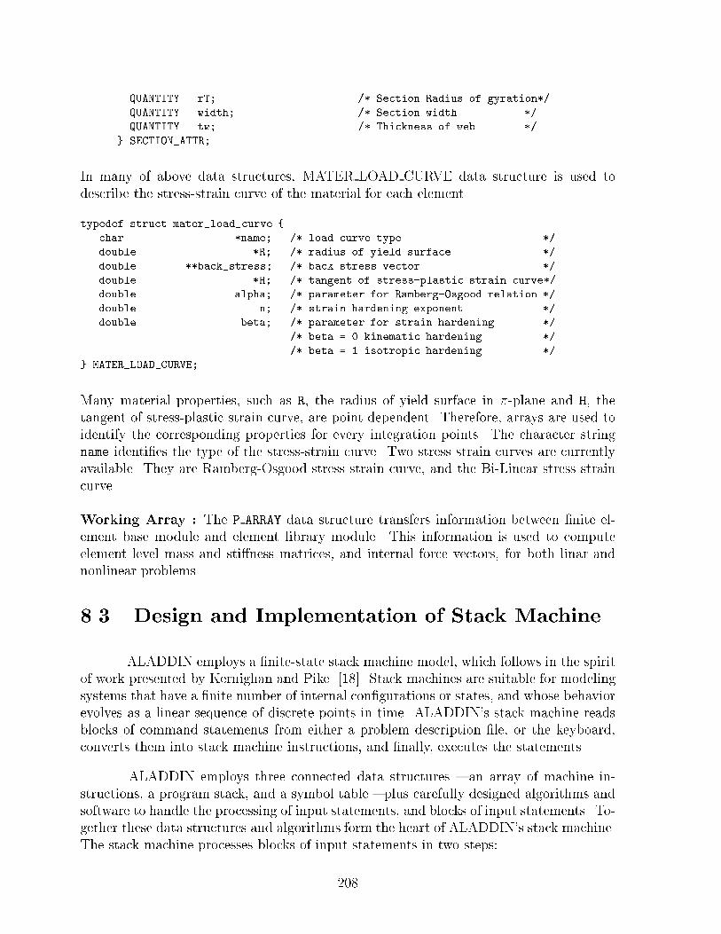
QUANTITY rT; /* Section Radius of gyration*/QUANTITY width; /* Section width */QUANTITY tw; /* Thickness of web */} SECTION_ATTR;In many of above data structures, MATER LOAD CURVE data structure is used todescribe the stress-strain curve of the material for each element.typedef struct mater_load_curve {char *name; /* load curve type */double *R; /* radius of yield surface */double **back_stress; /* back stress vector */double *H; /* tangent of stress-plastic strain curve*/double alpha; /* parameter for Ramberg-Osgood relation */double n; /* strain hardening exponent */double beta; /* parameter for strain hardening *//* beta = 0 kinematic hardening *//* beta = 1 isotropic hardening */} MATER_LOAD_CURVE;Many material properties, such as R, the radius of yield surface in �-plane and H, thetangent of stress-plastic strain curve, are point dependent. Therefore, arrays are used toidentify the corresponding properties for every integration points. The character stringname identi�es the type of the stress-strain curve. Two stress strain curves are currentlyavailable. They are Ramberg-Osgood stress strain curve, and the Bi-Linear stress straincurve.Working Array : The P ARRAY data structure transfers information between �nite el-ement base module and element library module. This information is used to computeelement level mass and sti�ness matrices, and internal force vectors, for both linar andnonlinear problems.8.3 Design and Implementation of Stack MachineALADDIN employs a �nite-state stack machine model, which follows in the spiritof work presented by Kernighan and Pike [18]. Stack machines are suitable for modelingsystems that have a �nite number of internal con�gurations or states, and whose behaviorevolves as a linear sequence of discrete points in time. ALADDIN's stack machine readsblocks of command statements from either a problem description �le, or the keyboard,converts them into stack machine instructions, and �nally, executes the statements.ALADDIN employs three connected data structures { an array of machine in-structions, a program stack, and a symbol table { plus carefully designed algorithms andsoftware to handle the processing of input statements, and blocks of input statements. To-gether these data structures and algorithms form the heart of ALADDIN's stack machine.The stack machine processes blocks of input statements in two steps:208

pc stackp data strcturequantity

built in functions data strcturematrix

.............

Inst 1

Inst 2

Inst 3

Inst 4

Data 1

Data 2

Data 3

Data 4

Stack

ptr to funcs

double

char string

section ptr

material ptr

elmt_attr ptr

Symbol 4 Symbol 5 Symbol 6

Array of Machine Instructions

ptr to funcs

double

char string

section ptr

Symbol 3

material ptr

elmt_attr ptr

Symbol 1 Symbol 2Symbol Table

Figure 8.2: Data Structures in ALADDIN's Stack Machine[1] Parse the input statement (or block of statements), and construct an array of machineinstructions. Groups of machine instructions are composed of calls to functions, plusinstructions to push and pop data and operands to/from the program stack.[2] Step through the array of machine instructions, and execute the functions pointed toby the machine instructions.Figure 8.2 is a simpli�ed schematic of the stack machines participating data structures,and their connectivity.Array of Machine Instructions : The array of machine instructions and programstack are declared with the following C statements:/* Define array of machine instructions */typedef int (*Inst)();#define STOP (Inst) 0; 209

#define NPROG 5000;Inst prog [ NPROG ];Inst *progp;Inst *pc;/* Define data structure for program stack */typedef union Datum {QUANTITY *q;MATRIX *m;SYMBOL *sym;} DATUM;#define NSTACK 500;static DATUM stack [ NSTACK ];The C statement Inst prog [ 5000 ] allocates memory for the array of machine in-structions. Each element of prog is a pointer of type int. Variables *progp and *pc arepointers of type Inst, which will be used to track elements in the array of instructions.The data structure DATUM is a union of pointers to quantity, matrix and symboltable items. Each element of the program stack is either a pointer to a quantity, a pointerto a matrix, or a pointer to a symbol table entry. The C statement static DATUM [ 500] allocates a block of memory for the program stack containing 500 elements of structureDATUM. The C function Code() plays a central role in the assembly of machine instructions.For example, the function call Code(Push); will add to the machine array, an elementcontaining a pointer to function Push(), and then increments the program pointer progp./** =====================================================================* The function code() builds up the machine stack prog, adding data* types Inst to it. The arguments to code() are pointers* to the functions defined later on in code.c, and pointers to* data types SYMBOL, which have been coerced by the use of the* cast Inst.* =====================================================================*/Inst *Code( Inst f ){Inst *oprogp = progp;if(progp >= &prog[NPROG])ExecutionError("ERROR >> program too big", (char *) 0);*progp++ = f;return oprogp;} 210

/** =====================================================================* Push DATUM d onto the stack, and increment stackp to next element.* =====================================================================*/Push( DATUM d ){ if(stackp >= &stack[NSTACK])ExecutionError("ERROR >> stack overflow", (char *) 0);*stackp++ = d; /* *stackp=d; stackp++; */}In functions Code() and Push(), ExecutionError() is a function that reports run-timeexecution errors in the interpretation of input commands (e.g over ows of the programstack). Function Code() has a single argument; the function call Code (Push); will, forexample, add to the machine array, an instruction to call function Push().Execution of Program Stack : An execution pointer marches along the machine arrayand implements the instruction set assembled during step [1] of the input process. Themachine instructions will push and pop items to/from the program stack, and call externalC functions as directed by the arguments to Code(...).Execute(p)Inst *p;{ for (pc = p; *pc = STOP; ) {pc = pc + 1;if( Check_Break() != 0) break;(*(*(pc-1)))();}}The code generated during parsing has been carefully arranged so that a STOP com-mand terminates each sequence of instructions that should be handled by a single call toExecute().8.3.1 Example of Machine Stack ExecutionWe now demonstrate use of the stack machine by working step-by-step throughthe details of processing the assignment x = 2 in;. We assume that Step [1] of the inputprocess is complete, with the array of machine instructions taking the values shown onthe left-hand side of Figure 8.3. During Step [1] of the input process, the YACC parser {details to be described in the next section { recognizes that x is a variable with data typeVAR, and 2 in as a quantity with number 2 and a units dimension in. The grammaticalrule for assignment (i.e. "=") has right associativity. Hence, when the machine is executed,211

..............

Symbol 2

name:

u.value: 2

u.q->dimen

type:NUMBER

Symbol 1

..............

units_name:

scale_factor: 1.0

units_type : SI_US

..............

u.q->dimen

u.value:

type: VAR

name: x

Symbol 9

Symbol 3

..............

units_name: in

units_type : US

scale_factor: 1.0

Symbol 6

value

dimen

quantity

..............

units_name: in

units_type : US

scale_factor: 1.0

units_name: in

scale_factor: 1.0

units_type : SI_US

..............

d1

d2

d3

..............

(Inst)

(Inst) Push_constant

(Inst)

(Inst) Dimension_Eval

(Inst) Push_Variable

(Inst) STOP

(Inst) Pop

(Inst)

(Inst) Push_Dimension

Symbol 7 Symbol 8sym 9

sym 4Symbol 5

..............

u.q->dimen

u.value:type:

name:

Symbol 4

sym 2

Machine ArrayStack

SymbolTable

Figure 8.3: Schematic of Machine and Stack for x = 2 in2 in will be pushed onto the stack �rst, and in two steps; �rst the unit in is pushed, andthen the number 2.Detailed snapshots of the program operation for Step [2] of the processing arelocated at the end of this subsection. The step-by-step procedure for execution of thestack machine is:[1] Push symbol table pointer onto stack for the variable in.[2] Push a constant 2 onto the stack.[3] Pop both 2 and in o� the stack, and combine them into a single quantity 2 in. Thequantity is pushed back onto the stack.[4] Push onto the stack, the symbol table pointer to variable x.[5] Pop x and 2 in from the stack. Assign 2 in to x and push x back onto the stack.[6] Data x is popped and cleared from the stack.Figures 8.4 to 8.9 show the relevant details of the machine array, symbol table, andprogram stack for Steps [1] to [6], respectively. In each of these �gures, pc is a programcounter that points to elements in the array of machine instructions { the elements of the212

machine array are pointers to C functions. The dashed and solid arrows represent the twostages of the pc positions. As detailed in the C function Execute(), and shown in Figure8.4, program counter pc initially points to (Inst) Push Dimension. The position of pcis represented by the (dotted) left-to-right arrow in Figure 8.4. Notice, however, that pcis incremented to the (solid) arrow position (i.e pc = pc+1) before Push Dimension() iscalled. Now (pc-1) points at (Inst) Push Dimension. The details of Push Dimension()are as follows:/** =======================================================* Push_Dimension() : push dimensioned quantity onto stack* =======================================================*/void Push_Dimension(){DATUM d;int length;d.q = (QUANTITY *) MyCalloc(1,sizeof(QUANTITY));d.q->dimen = NULL;d.q->value = ((SYMBOL *) *pc)->u.q->value;pc = pc + 1;Push(d);}The machine instruction at the new value of pc points to a quantity stored in the symboltable. Push Dimension() allocates memory of a new quantity (given by d.q), and copiesto it, the contents of the symbol table entry. The result is pushed onto the program stack.After unit in and number 2 are both pushed onto stack (i.e. d1 and d2 on thestack shown in Figure 8.3), function Dimension Eval() pops d1 and d2 from the stack,assigns the units in to number 2, and produces the quantity 2 in back onto the stack.Next, the symbol table pointer for variable x is pushed onto the stack by C functionPush Variable(). Details of this step are shown in Figure 8.7.The C function Assign Quantity() assigns the quantity 2 in to variable x, andpushes the new x onto stack. Details of this step are shown in Figure 8.8. The second-to-last machine instruction pops the last item from the stack, as shown in Figure 8.9.Finally, (Inst) STOP, halts the looping mechanism in C function Execute().213

quantityvaluedimen

units_name: inunits_type : USscale_factor: 1.0

..............

(Inst) Push_constant(Inst) (Inst) Dimension_Eval

(Inst) Push_Variable

(Inst) Push_Dimension

(Inst) STOP

(Inst) Pop

(Inst) (Inst) Assign_Quantity

(Inst)

Machine Array

Stack

d1

pc = pc+1pc -1 Push_Dimension(): Push "in" onto stack

name: type:

..............u.q->dimen

u.value:

Symbol 1

units_name: inunits_type : USscale_factor: 1.0

..............

Figure 8.4: Step 1 { Push Unit onto Stack(Inst) Push_constant

(Inst) Dimension_Eval

(Inst) Push_Variable

(Inst)

(Inst) Push_Dimension

(Inst)

Stack

(Inst) STOP

(Inst) Pop

(Inst) Assign_Quantity

d1d2

(Inst)

Machine Array

pc = pc+1

pc -1

quantityvalue

dimenunits_name: in

units_type : US

scale_factor: 1.0..............

name:

..............u.q->dimen

Symbol 2

type: NUMBERu.value: 2

..............

units_name:

units_type : SI_USscale_factor: 1.0

Push_Constant(): Push constant " 2" onto stack

Figure 8.5: Step 2 { Push Number onto Stack214

Dimension_Eval(): Pop out d2 and d1 from stack combine "2" and "in" into one quantity, d, and Push d back to stack

Stack

d1

d2

Pop d2, Pop d1, Push d

Stack

d

units_name: in

units_type : US

scale_factor: 1.0..............

(Inst) Push_constant

(Inst) Dimension_Eval

(Inst) Push_Variable

(Inst)

(Inst) Push_Dimension

(Inst)

(Inst)

(Inst) STOP

(Inst) Pop

(Inst) Assign_Quantity

Machine Array

pc = pc + 1pc -1

quantity

value: 2

dimen

Figure 8.6: Step 3 { Combine Number and Unit into Quantity

scale_factor: 1.0..............

units_name: units_type : SI_US..............

u.q->dimen

Symbol 3name: xtype: VARu.value:

(Inst) Push_Dimension

Stackunits_name: inunits_type : USscale_factor: 1.0

..............

dd3

quantity

dimen

value: 2

Push_Variable(): Push symbole table pointer

(Inst) Pop

(Inst) STOP

(Inst) Assign_Quantity

(Inst)

(Inst) Push_Variable

(Inst) Dimension_Eval

(Inst)

(Inst) Push_constant

(Inst)

onto stack for the variable "x"

Machine Array

pc = pc+1pc -1

Figure 8.7: Step 4 { Push Variable onto Stack215

..............

Symbol 3

name: xtype: QUANTITY

u.value: 2

u.q->dimen

units_name: in

units_type : US

scale_factor: 1.0..............

Stack

d4

(Inst) Push_constant

(Inst)

(Inst) Dimension_Eval

(Inst) Push_Variable

(Inst) Push_Dimension

(Inst)

(Inst) STOP

(Inst) Pop

(Inst)

(Inst) Assign_Quantity

Stack

d3d

Assign_Quantity (): Pop out d3 and d from stack, assign " 2in" in d, to "x" in d3, store new datain d4 and push d4 back to stack

Pop d3, Pop d and Push d4

Machine Array

pc = pc+1pc-1

Figure 8.8: Step 5 { Assign Quantity to VariableStack Stack

d4

Pop d4

(Inst) Push_constant

(Inst)

(Inst) Dimension_Eval

(Inst) Push_Variable

(Inst) Push_Dimension

(Inst)

(Inst) STOP

(Inst) Pop

(Inst)

(Inst) Assign_Quantity

Machine Array

pc = pc+1 Pop (): Pop out . Clear top data from stack

pc-1

Figure 8.9: Step 6 { Clear Top Data from Stack216

8.4 Language Design and ImplementationWe have used the UNIX tool YACC (an acronym for Yet Another CompilerCompiler [16]) to de�ne a language for the de�nition and solution of matrix and �niteelement problems. For gentle introductions to YACC, see Chapter 8 of Kernighan andPike [18], and the O'Reilly text by Levine et al. [21]. For a theoretical discussion on LRparsers, see Aho et al. [2].In ALADDIN, the details of the YACC grammar and associated C code are locatedin a �le called grammar.y, which is partitioned into four parts:%{Part 1 : Optional C statement, declaration;%}Part 2 : YACC declarations, lexical tokens, grammar variable, precedenceand associativity information%%Part 3 : Grammar rules and semantic actions%%Part 4 : Lexical analysis with a C function called yylex().YACC takes the speci�cations in Parts 1 to 3, and generates a C code function calledyyparse() for: (a) the matching of tokens and their types against the grammatical rulesof the language, and (b) the handling of semantic actions.Part 4 : In Part 4 of the YACC speci�cation, we write a C function called yylex() toscan streams of input characters, and identify token names and their types. The namesand types of tokens are passed onto yyparse() for the matching against grammaticalrules. Here is an abbreviated version of yylex():yylex(){double value;int finished;/* [a] : Eat blank space, tab, and newline input. Read comment statements */while((c = fgetc(fin)) == ' ' || c == '\t' || c == '\n' || c == '/') {if(c == '\n')lineno++;if(fin == stdin && finp != stdin) {if(c == '\n') {printf("ALADDIN :");fflush(stdout);}fputc(c, finp);} 217

if(c == '/') {if(follow('*', TRUE, FALSE) == TRUE) {c = fgetc(fin);finished = FALSE;while(finished == FALSE) {c = fgetc(fin);if(c == '\n')lineno++;if(c == EOF)FatalError("ERROR >> ... file ended with unbalanced comment !!\n",(char *)NULL);if((c == '*') && (follow('/', TRUE, FALSE) == TRUE)) {finished = TRUE;}}} else {return c;}}}/* [b] : return end-of-file */if(c == EOF) {return END_OF_FILE;}/* [c] : read and store floating-point numbers */if (c == '.' || isdigit(c)) {ungetc(c, fin);fscanf(fin, "%lf", &value);if(fin == stdin && finp != stdin) fprintf(finp, "%lf", value);yylval.sym = build_table("", NUMBER, value);return NUMBER;}/* [d] : read and store variable */if (isalpha(c) || c == '_') {SYMBOL *s;char sbuf[100], *p = sbuf;do {if(p >= sbuf + sizeof(sbuf) - 1) {p = '\0';ExecutionError("ERROR >> name too long");}*p++ = c; 218

} while ((( c = fgetc(fin)) != EOF) && (isalnum(c) || (c == '_' )));ungetc(c, fin);*p = '\0';if(fin == stdin && finp != stdin) fprintf(finp, "%s", sbuf);if ((s = lookup(sbuf)) == 0) {s = build_table(sbuf, VAR, 0.0);}yylval.sym = s;switch((int) s->type) {case UNDEF: case VAR: case QUAN:return VAR;default:return (s->type);}}/* [e] : Get Quoted String */if (c == '"') {char sbuf[100], *p;if(fin == stdin && finp != stdin) fputc(c, finp);for(p = sbuf; (c = fgetc(fin)) != '"'; p++) {if(c == '\n' || c == EOF)ExecutionError("ERROR >> missing quote");if(p >= sbuf + sizeof(sbuf) - 1) {p = '\0';ExecutionError("ERROR >> string name too long");}if((fin == stdin && finp != stdin))fputc(c, finp);*p = backslash(c);}*p = 0;yylval.sym = (SYMBOL *) SaveString(sbuf);if(fin == stdin && finp != stdin)fputc(c, finp);return STRING;}if(fin == stdin && finp != stdin) {fputc(c, finp);}switch(c) {case '>': 219

return follow('=', GE, GT);case '<':return follow('=', LE, LT);case '=':return follow('=', EQ, '=');case '!':return follow('=', NE, NOT);case '|':return follow('|', OR, '|');case '&':return follow('&', AND, '&');default:return c;}}Here we emphasize only the main components of yylex(). yylex() scans streams of inputand automatically removes black spaces, tabs, and all input between comment statements.Numbers must begin with either a digit of a decimal point { they are temporarily storedin ALADDIN's symbol table. Character strings are enclosed within quotes (i.e "....").Variables and built-in function names are alphanumeric strings that must begin witha character { the details of keywords in ALADDIN's programming language are storedin the symbol table. Finally, yylex() identi�es token types for two-character sequencesused in relational and logical operators. The interested reader should consult the programsource code for details on functions backslash(), follow(), warning(), and so on. Nowlet's look at the details for our stack machine:Part 1 : We use the macro declarations%{...#define Code2(c1,c2) Code(c1); Code(c2)#define Code3(c1,c2,c3) Code(c1); Code(c2); Code(c3)...%}as short form for calls to function Code().Part 2 : The YACC declarations begins with character %.%union {SYMBOL_PTR sym;Inst *inst;int narg;}%token <sym> NUMBER%token <sym> VAR%type <inst> quantity%type <inst> dimensions%left '+' '-' /* left associative, same precedence */%left '*' '/' /* left associative, higher precedence */%right '^' /* right associative, higher precedence */220

The union declares that YACC stack may holds three di�erent types of elements; a pointerto an item in the symbol table, a machine instruction pointer, and an integer narg torepresent the number of arguments in a function. The token declaration with arguements< sym > says that NUMBER and VAR will be input tokens accessed by dereferencing asymbol table pointer. In ALADDIN, NUMBER and VAR are integers generated by YACC torepresent value of type double and character strings, respectively. The type declarationspeci�es that quantity and dimensions will be machine instructions.The left and right keywords specify left and right associativity of operators,respectively. In YACC, the precedence of operators is de�ned by order of appearance,with tokens in the same declaration having equal precedence. Tokens appearing at theend of the declaration list have higher precedence than those at the beginning. Therefore,the operators + and - are left associative, and in the same precedence level. The multiplyand divide operators have equal precedence, and are left associative. They have higherprecedence than the add and subtract operators. The power \̂" operator has the highestprecedence level, and is right associative.Part 3 : Grammatical Rules : ALADDIN has more than 100 grammatical rules.Rather than attempt to explain all of them here, we will concentrate only on those rulesneeded to match simple assignment statements, to identify matrices, and last, generate afor-looping construct. We begin with the collection of rules needed to recognize "2", "2in", "(2 in)" and "2 in + 3 in".%%quantity: NUMBER { $$ = Code2(Push_Dimensionless, (Inst) $1); /* rule 1 */Code2(Push_Constant, (Inst)$1);Code(Dimension_Eval); };%%Number 2 is a digit. It is assigned type NUMBER in yylex(). A stream of input thatconsists of a number alone is matched by rule 1 of the grammar. A number without unitsis considered to be a quantity (i.e see left-hand side of rule 1). The name $$ refers tovalue of the symbol to the left of the colon { in this case quantity. The semantic actionsfor rule 1 are a series of machine instructions, via calls to Code(), to push a dimensionlessquantity onto the program stack, push a constant onto the program stack, and �nally,evaluate the result.We now introduce rules of the grammar designed to parse units expressions of theform in2, in � in, lb � in, in=sec2, and so on. The grammatical rules are:dimensions: DIMENSION { $$ = Code( Push_Dimension); /* rule 2 */Code( (Inst)$1 ); }| '(' dimensions ')' { $$ = $2; } /* rule 3 */| dimensions '*' dimensions { Code( Dimension_Mult ); } /* rule 4 */221

| dimensions '/' dimensions { Code( Dimension_Div); } /* rule 5 */| dimensions '^' quantity { $$ = $1; /* rule 6 */Code( Dimension_Power ); };YACC uses the vertical bar symbol \j" to separate individual rules in a group { the symbolshould be interpreted as meaning or. Semantic actions are included inside the f g). Theinput streams 2 in and (2 in) are considered are of type quantity,quantity: NUMBER dimensions { Code2(Push_Constant, (Inst)$1);Code(Dimension_Eval); $$ = $2;} /* rule 7 */| '(' quantity ')' { $$ = $2; } /* rule 8 */;and are matched by rules 7 and 8. More precisely, (2 in) is �rst matched by rule 8, andthen by rule 7. The units are speci�ed by type dimension.With the rules for recognizing a quantity in place, it is relatively straight forwardto de�ne grammatical rules for arithmetic operations on quantities. In the input command2 in + 3 in, the quantities 2 in and 3 in are �rst recognized by rule 7, and the additionof quantities by the rule 9.%%quantity: quantity '+' quantity { Code(Quantity_Add); } /* rule 9 */%%The C code located in function Quantity Add() takes care of the appropriate stack oper-ations. Similar rules are written for subtraction of two quantities (rule 10), multiplicationof two quantities (rule 11), and division of quantities (rule 12). A quantity raised to thepower of another quantity is considered to be a quantity (rule 13).%%quantity : quantity '-' quantity { Code(Quantity_Sub); } /* rule 10 */| quantity '*' quantity { Code(Quantity_Mul); } /* rule 11 */| quantity '/' quantity { Code(Quantity_Div); } /* rule 12 */| quantity '^' quantity { Code(Quantity_Power);} /* rule 13 */;%%Again, Quantity Sub(), Quantity Mul() and so on, are C functions for arithmetic ofquantities with appropriate pushing and popping of data items to/from ALADDIN'sprogram stack. Input commands, such as x = 3 in and y = 2 in + x involve the as-signment of a quantity to a variable. Both cases can be represented the rule:%%quantity : VAR '=' quantity { Code2( Push_Variable, (Inst)$1); /* rule 14 */Code( Assign_Quantity); $$ = $3; };%% 222

Using the rules stated above, 3 in is recognized as a quantity, and x is a variable type.The complete input x = 3 in is matched by rule 14. Moreover, because YACC rules arerecursively de�ned, 2 in + x is matched by rule 9. Parser trees for the statements x =3 in followed by y = 2 in + x are shown in Figure 8.10.Quantity

VAR Quantity

Quantity

Quantity

Quantity Quantity

VAR

NUMBER

NUMBER Dimension

Dimension

x 3 in

y = 2 in + x

=

Figure 8.10: Parser Trees for x = 3 in and y = 2 in + xMatrix Generation : As pointed out in the previous chapters, two mechanisms exist forthe generation of matrices; de�nition of matrices from input, and generation of matricesvia built-in matrix functions. We will begin with the latter (e.g. as in A = Zero([2,3]);).%token <sym> MATX%%matrix : MATX {$$ = Code( Push_Matrix ); /* M_rule 1 */Code( (Inst)$1 );Code( Matrix_Eval );%%YACC uses the variable type MATX to represent variables of type matrix. The seman-tic action that follows identi�cation of a matrix has two key parts { the C functionPush Matrix() pushes a pointer to the symbol table entry containing the matrix ontothe program stack. Matrix Eval() pops the matrix pointer from the stack, allocatesmemory for a new matrix, and copies the contents of the symbol table matrix to the newmatrix. Finally, a pointer to the new matrix is pushed onto the stack.223

The second approach is to generate matrices directly from keyboard/�le input.Matrices generated directly from input are de�ned as series of quantities inside []. Con-sider, for example, the 2x2 matrix: " 2 33 5 #which may also be represented as [ 2 , 3 ; 3, 5 ]. A matrix row is simply a list of quantitiesseparated by commas. Individual matrix rows are separated by semicolons. The YACCgrammar for identifying matrices is:%type <narg> matrix_seq%type <narg> quantity_row%%matrix : '[' matrix_seq ']' {$$ = Code( Push_Variable );Code( (Inst)$2 );Code( Matrix_Build);} /* M_rule 2 */;matrix_seq: quantity_row { Code( Push_Variable );Code( (Inst)$1 );$$ = 1; } /* M_rule 3 */| matrix_seq ';' quantity_row { Code2( Push_Variable );Code( (Inst)$3 );$$ = $1 + 1;} /* M_rule 4 */;where type speci�es that matrix seq and quantity row are of type < narg>. matrix seqrecords number of rows and the number is pushed onto stack { this is done by M rule 3and M rule 4. As soon as row of quantities is identi�ed, matrix seq is initialized withnumber = 1 (M rule 2). Then, matrix seq is increased by 1 for each semicolon \;" thatis parsed, with the sum being accumulated recursively via M rule 4. Within each row,columns separated by commas (",") are quantities.quantity_row: { $$ = 0; }| quantity { $$ = 1; } /* QR_rule 1 */| quantity_row ',' quantity { $$ = $1 + 1;} /* QR_rule 2 */;Similarly, the number of columns in a matrix is recorded by quantity row.Matrix Operations : The grammatical rules for matrix operations are similar to thoseof engineering quantities.| matrix '*' matrix {Code( Bltin_Matrix_Mult);} /* M_rule 5 */| matrix '+' matrix {Code( Bltin_Matrix_Add);} /* M_rule 6 */| matrix '-' matrix {Code( Bltin_Matrix_Sub);} /* M_rule 7 */| '(' matrix ')' {$$ = $2;} /* M_rule 8 */| quantity '*' matrix {Code( Bltin_Quan_Matrix_Mult);224

$$ = $3;} /* M_rule 9 */| matrix '*' quantity {Code( Bltin_Matrix_Quan_Mult);} /* M_rule 10 */| matrix '/' quantity {Code( Bltin_Matrix_Quan_Div);} /* M_rule 11 */;These rules generate an array of machine instructions for matrix addition, subtractionand multiplication (i.e. M rule 5, M rule 6 and M rule 7). They allow for the parsingof a matrix inside parentheses (M rule 8), the multiplication of a quantity times a matrix(M rule 9), a matrix times a quantity (M rule 10), and a matrix divided by a quantity(M rule 11).For Looping Construct : The development of a YACC grammar and supporting Ccode for looping and branching constructs is the most complicated part of ALADDIN'sprogramming language. A description of the while-looping construct may be found inChapter 8 of Kernighan and Pike [18]. The purpose of this subsection is to explain ourimplementation of the for-looping construct. The family of grammatical rules:stmt: for '(' exprlist ';' cond ';' exprlist ')' stmt end { /* F_rule 0 */($1)[1] = (Inst) $3; /* initiation F_rule 1 */($1)[2] = (Inst) $5; /* condition F_rule 2 */($1)[3] = (Inst) $9; /* body of loop F_rule 3 */($1)[4] = (Inst) $7; /* increments F_rule 4 */($1)[5] = (Inst) $10; /* end, if cond fails F_rule 5 */};for: FOR { $$ = Code3( For_Code, STOP, STOP); Code2(STOP, STOP); Code(STOP);};exprlist: listlist { Code(STOP); $$ = $1; };listlist : { $$ = progp; } /* L_rule 1 */| quantity /* L_rule 2 */| listlist ',' quantity /* L_rule 3 */;cond: quantity { Code(STOP); $$ = $1; };assumes that memory in the array of machine instructions will take a form as shown inFigure 8.11. A for-loop is simply a statement (stmt). The initiation and incrementalsteps of the for-loop are expressed as exprlists, which are themselves subdivided intolistlist. A listlist could be a space (nothing) (L rule 1), an engineering quantity(L rule 2), or a series of quantities separated with \," (L rule 3). The body of a for-loopis also a statement(stmt) { this rule allows for the nesting of for-loop constructs. Thecondition part of the for loop is an engineering quantity.After the token FOR has been recognized, �ve spaces in the array of machineinstructions are reserved for the storage of pointers to the initiation code (F rule 1), the225

(Inst) For_Code

..............

..............

(Inst) STOP

..............

(Inst) STOP

..............

..............

(Inst) STOP

stmt

listlist

cond

listlistinitialization

condition

increment

body of for-loop

end, if condition fails(Inst) STOP

next stmt

Machine Stack

Figure 8.11: Machine Stack for For-Loop Constructcondition (F rule 2), the incremental steps (F rule 3), the body of the for-loop (F rule4) and the STOP instruction (F rule 5). The two character sequence refers $n refersto the value of a type stacked n spaces beyond the current namelist production. In thisparticular case, $1 is the location in the machine of the token identi�ed by F rule 0. Theinitiation, condition, body, increments, and end components of the for loop are access bymachine array elements ($1)[1] to ($1)[5], respectively. For the sake of completeness,we now include the C code for For Code().For_Code(){DATUM d;Inst *savepc = pc;Execute(*((Inst **) savepc)) ; /* initiation */Execute(*((Inst **) (savepc+1))) ; /* cond */d = Pop();while(d.q->value) {if(Check_Break()) break;Execute(*((Inst **)(savepc+2))); /* body of loop */Execute(*((Inst **)(savepc+3))); /* increments */if(returning || Check_Break()) break;Execute(*((Inst **) (savepc+1))) ; /* cond */if( CheckUnits()== ON ) { 226

free((char *)d.q->dimen->units_name);free((char *)d.q->dimen);free((char *)d.q);}d = Pop();}if(!returning)pc = *((Inst **)(savepc + 4)); /* next statement */After_Break();}Notice how the layout of memory in Figure 8.11 has been carefully combined with functioncalls to Execute().

227

Part VCONCLUSIONS AND FUTUREWORK

228

Chapter 9Conclusions and Future Work9.1 ConclusionsIn the general area of computational technology for engineering, the 1990's areshaping up to be the decade of global networking and multimedia. These advances willallow for the prototyping of interactive computing environments tailored to the life cycledevelopment of complex engineering systems. For these environments to be commerciallysuccessful, they will need to support development of engineering systems from multipleviewpoints, and at multiple levels of abstraction. Engineers should be provided withthe tools to integrate once disparate disparate disciplines. While the merging of matrixcomputations with �nite elements, optimization, and graphics is already evident, manyother possibilities exist. For instance, now that many companies are engaging in businesspractices that are geographically dispersed, engineers will soon expect connectivity toa wide range of information services { electronic contract negotations, management ofproject requirements, design rule checking over the Internet, and availability of materialsand construction services are likely candidates. The participating computer programsand networking infrastructure will need to be fast and accurate, exible, reliable, and ofcourse, easy to use [12, 28].Our long-term goal for ALADDIN is to provide engineers with such a computa-tional problem-solving environment. Version 1.0 of ALADDIN is simply a �rst step inthis direction, and is much less ambitious. The emphasis in development has so far beenon the basic system speci�cation, and its application to matrix and �nite element prob-lems. We have tried to determine what data types, control structures, and functions willallow engineers to solve a wide variety of problems, without the language becoming toolarge and complicated, and without extensibility of the system being compromised. Ourstrategy for achieving the latter objective is described in Chapter 1. The test applicationshave been taken from traditional Civil Engineering, and have focussed on the design andanalysis of highway bridges and earthquake-resistant buildings.ALADDIN (Version 1.0) is approximately 36,000 lines of C, and getting the pro-gram to this point has taken approximately three years of part-time work. We have229

written nearly all of the source code from scratch { along the way, a new data structurefor the matrices with units was designed and software implemented. Many of the matrixalgorithms that ALADDIN uses are documented in the forthcoming text of Austin andMazzoni [5]. The language design must be followed by entensive testing of the softwarewith matrix and �nite element test problems that are complicated enough to push thelimits of the software (Note : In our experience, many coding errors will not show up intrivial engineering applications).As the work on ALADDIN progressed, we occasionally identi�ed small extensionsto the language that would allow ALADDIN to attack a new problem area. When thelanguage for ALADDIN was �rst designed we did not have design rule checking in mind,for example. Yet once the basic matrix and function language speci�cation was in place,and the �nite element analyses worked, only a couple of extra functions were needed forthe implementation of basic design rule checking.Together these observations lead us to believe that our goal of keeping the AL-ADDIN language small and extensible has been achieved. This work lays the foundationfor many avenues of future work.9.2 Future WorkFigure 9.1 is a schematic of the current components of work, plus modules of workthat are needed for the next extension of ALADDIN. The future work should focus on:[1] Nonlinear Algorithms : The scope of applications in this report has been restrictedto time-dependent analysis of linear structural systems. Future work should extendthis work to the time-history analysis of systems having material and geometricnonlinearities. A �rst step in this direction is reported in Chen and Austin [10].[2] User-defined Functions : Version 1.0 of ALADDIN does not permit the use ofuser-de�ned functions and procedures in the input �le. When we �rst began workingon ALADDIN, our feeling was that the input �le language should be relatively simple{ otherwise, why not simply code the whole problem in C ? An easy way of controlinglanguage complexity is to disallow user-de�ned functions in the input �le, and thisis what we have done for ALADDIN Version 1.0. Now that the matrix and �niteelement libraries are working, this early decision needs to be revised. We would liketo combine the �nite element analysis with discrete simulated annealing optimizationalgorithms, along the lines proposed by Kirkpatrick [19]. The latter could besuccinctly implemented if user-de�ned functions were available. The current versionof ALADDIN assumes that all user-de�ned variables are global. When user-de�nedfunctions are added to ALADDIN, notions of scope should also be added to variables(this could be implemented via an array of Symbol Tables).[3] Graphical Library : An obvious limitation of ALADDIN (Version 1.0) is that itlacks a graphical user interface. Providing a suitable interface is easier said than230

FINITE ELEMENT LIBRARY

MATRIX LIBRARY

OPTIMIZATION LIBRARY

FUTURE WORKSCOPE OF THIS REPORT

ALADDIN’S KERNEL AND INPUT FILES

INPUT FILE

Block of input statements....

Block of input statements....

Block of input statements....

Block of input statements....

GRAPHICS LIBRARY

[ STACK MACHINE ]

ALADDIN’S KERNEL.

LIBRARIES OF BUILT-IN C FUNCTIONS

Figure 9.1: Future Development for ALADDINdone. If ALADDIN simply preported to conduct �nite element analysis, then itwould be a relatively easy process to code-up an interactive pre- and post-�niteelement processor in X windows (or a suitable PC graphics package).The problem with this approach is that it only serves one half of ALADDIN's capa-bilities { in addition to graphically describing the �nite element mesh and modelingassumptions, a graphical interface should also provide a graphical counterpart tothe solution algorithm speci�cations (e.g. Newmark Integration). We will explorethe use of visual programming languages to see if they are suitable for this purpose.[4] Optimization Library : We would like to extend the language speci�cation so thatengineers can describe design objectives, design constraints, and design parameters,for general engineering optimization problems in a compact manner. The issue of\compactness" is particularly relevant for optimization problems that involve �niteelement analysis because they often contain hundreds, and sometimes thousands, ofconstraints. 231

Further work is needed to determine how groups of similar constraints can be bun-dled into groups, and how ALADDIN's control structures can be exploited to writedown these constraints in a compact manner. Once the issue of constraints is sortedout, the pathway for describing the design parameters and objectives should (hope-fully) become clearer.[5] Test Problem Suite : New suites of test problem �les will be needed as the detailsof items [2] and [4] are �lled in (please let us know if you �nd an error in one of thetest �les!).Version 1.0 of ALADDIN is basic in the sense that many features found in commer-cial �nite element codes have yet to be implemented in ALADDIN. For example, thecurrent version of ALADDIN only supports external loads applied at the nodes. Inthe near future we will add element level loads so that uniform loads can be appliedto two-dimensional problems, and pressure loads can be applied to the surface ofshell �nite elements in three-dimensional problems.[6] WWW Home Page : We are currently developing a World Wide Web (WWW) HomePage for ALADDIN. The ALADDIN home page will provide basic information onALADDIN, sample matrix and �nite element test problems, ALADDIN source code,and copies of this report. Our near-term plans are to experiment with the dynamicdocuments capabilities of WWW, and create home pages where WWW visitors caninteract with an ALADDIN script running at the University of Maryland.Work items [1] to [5] are tightly coupled. Understanding their interaction is an activearea of research.AcknowledgementsThis work has been supported in part by NSF Grant ECD-8803012, by NSF grantsto the Institute for Systems Research at the University of Maryland, and by a series offellowship grants to Wane-Jang Lin from the Federal Highway Administration.The early stages of this project would not have been possible without valuablediscussions with Dr. Bunu Alibe and Bert Davy, faculty members in the Department ofCivil Engineering at Morgan State University.

232

Bibliography[1] ABAQUS. Example Problems Manual, version 5.2. Hibbitt, Karlsson & Sorensen,Inc., Hibbitt, Karlsson & Sorensen, Inc., 1080 Main Str., Pawtuchet, RI 02860, 1992.[2] Aho A. V., Sethi R., Ullman J. D. Compilers : Principles, Techniques and Tools.Addison Wesley, 1985.[3] Austin M. A., Pister K. S., Mahin S. A. A Methodology for the ProbabilisticLimit States Design of Earthquake Resistant Structures. Journal of the StructuralDivision, ASCE, 113(8):1642{1659, August 1987.[4] Austin M. A., Pister K. S., Mahin S. A. Probabilistic Limit States Design of MomentResistant Frames Under Seismic Loading. Journal of the Structural Division, ASCE,113(8):1660{1677, August 1987.[5] Austin M.A., Mazzoni D. C Programming for Engineers. John-Wiley and Sons.(Scheduled for publication in 1996).[6] Balling R. J., Pister K. S., Polak E. DELIGHT.STRUCT: A Computer-AidedDesign Environment for Structural Engineering. Computer Methods in Applied Me-chanics and Engineering, pages 237{251, January 1983.[7] Bathe K. J. Numerical Methods in Finite Element Analysis. Prentice-Hall, Engle-wood Cli�s, N.J., 1976.[8] Bathe K. J. Finite Element Procedures in Engineering Analysis. Prentice-Hall,Englewood Cli�s, N.J., 1982.[9] Bathe K. J., Cimento, A. P. Some Practical Procedures for the Solution of NonlinearFinite Element Equations. Computer Methods in Applied Mechanics and Engineering,22:59{85, 1980.[10] Chen X.G., Austin M.A. Development of a Shell Finite Element for Project AL-ADDIN. Technical report, University of Maryland, College Park, MD. 20742, 1995.[11] Cmelik R.F., Gehani N.H. Dimensional Analysis with C++. IEEE Software, pages21{26, May 1988.[12] Gallopoulos E., Houstis E. Computer as a Thinker/Doer : Problem-Solving Envi-roments for Computational Science. IEEE Computational Science and Engineering,1(2):11{23, 1994. 233

[13] Gehani N.H. Databases and Units of Measure. IEEE Transactions on SoftwareEngineering, 8(6):605{611, November 1982.[14] Ghali A., Neville A.M. Structural Analysis : A Uni�ed and Matrix Approach.Chapman and Hall, 2nd Edition edition, 1979.[15] Jin Lanheng. Analysis and Evaluation of a Shell Finite Element with Drilling Degreeof Freedom. Technical report, University of Maryland, College Park, Maryland 20742,1994.[16] Johnson S. C. YACC - Yet another Compiler Compiler. Technical report, AT&TBell Laboratories, Murray Hill, New Jersey, 1975.[17] Karr M., Loveman D. B. Incorporating Units into Programming Languages. Com-munications of the ACM, 21(5):385{391, May 1978.[18] Kernighan B. W., Pike R. The UNIX Programming Environment. Prentice-HallSoftware Series, 1983.[19] Kirkpatrick S., Gelatt C.D., Vecchi M.P,. Optimization by Simulated Annealing.Science, 220(4598):671{680, May 1983.[20] Kronlof K. Method Integration : Concepts and Case Studies. John-Wiley and Sons,1993.[21] Levine J.R., Mason T., Brown D. Lex and Yacc. O'Reilly and Associates, Inc,1992.[22] Luenberger David G. Linear and Nonlinear Programming. Addison-Wesley Publish-ing Company, 1984.[23] Mondkar D. P., Powell G. H. ANSR - 1 General Purpose program for Analysis ofNonlinear Structural Response. Report No. EERC 75-37, Earthquake EngineeringResearch Center, December 1975.[24] Nye W. T., Riley D. C., Sangiovanni-Vincentelli A. L., Tits A. L. DE-LIGHT.SPICE: An Optimization-Based System for the Design of Integrated Circuits.IEEE Trans. CAD Integrated Circuits and Systems, CAD-7, pages 501{520, 1987.[25] Nye W. T., Tits A. L. An Application-Oriented, Optimization-Based Methodologyfor Interactive Design of Engineering Systems. International Journal of Control,43(6):1693{1721, 1986.[26] Nye W., Tits A. L. DELIGHT FOR BEGINNERS. Memorandum No. UCB/ERLM82/55, Department of Electrical Engineering, July 1982.[27] Salter K.G. A Methodology for Decomposing System Requirements into Data Pro-cessing Requirements. Proc. 2nd Int. Conf. on Software Engineering, 1976.234

[28] Tesler L.G. Networked Computing in the 1990's. Scienti�c American, 265(3):86{93,September 1991.[29] Wu T.L. DELIGHT.MIMO : An Interactive System for Optimization-Based Multi-variable Control System Design. Memorandum No. UCB/ERL M86/90, Departmentof Electrical Engineering, December 1986.[30] Zienkiewitz O.C., Taylor R.L. The Finite Element Method. McGraw-Hill, Inc, 1989.For details on FEAP, see Chapter 15.

235