alamode documentation
TRANSCRIPT

ALAMODE DocumentationRelease 1.3.0
Terumasa Tadano
Oct 06, 2021

Contents
1 Users Guide 11.1 About . . . . . . . . . . . . . . . . . . . . . . . . . . . . . . . . . . . . . . . . . . . . . . . . . . . 1
1.1.1 What is ALAMODE? . . . . . . . . . . . . . . . . . . . . . . . . . . . . . . . . . . . . . . 11.1.2 Features . . . . . . . . . . . . . . . . . . . . . . . . . . . . . . . . . . . . . . . . . . . . . 11.1.3 Links . . . . . . . . . . . . . . . . . . . . . . . . . . . . . . . . . . . . . . . . . . . . . . 21.1.4 License . . . . . . . . . . . . . . . . . . . . . . . . . . . . . . . . . . . . . . . . . . . . . 21.1.5 How to Cite ALAMODE . . . . . . . . . . . . . . . . . . . . . . . . . . . . . . . . . . . . 21.1.6 Issues & Bug report . . . . . . . . . . . . . . . . . . . . . . . . . . . . . . . . . . . . . . . 31.1.7 Acknowledgment . . . . . . . . . . . . . . . . . . . . . . . . . . . . . . . . . . . . . . . . 31.1.8 Author & Contact . . . . . . . . . . . . . . . . . . . . . . . . . . . . . . . . . . . . . . . . 3
1.2 Download . . . . . . . . . . . . . . . . . . . . . . . . . . . . . . . . . . . . . . . . . . . . . . . . . 31.3 Installation . . . . . . . . . . . . . . . . . . . . . . . . . . . . . . . . . . . . . . . . . . . . . . . . 3
1.3.1 Requirement . . . . . . . . . . . . . . . . . . . . . . . . . . . . . . . . . . . . . . . . . . 31.3.2 Install using conda (recommended for non-experts) . . . . . . . . . . . . . . . . . . . . . . 41.3.3 Install using native environment (optional for experts) . . . . . . . . . . . . . . . . . . . . . 6
1.4 Running ALAMODE . . . . . . . . . . . . . . . . . . . . . . . . . . . . . . . . . . . . . . . . . . 91.4.1 Program alm . . . . . . . . . . . . . . . . . . . . . . . . . . . . . . . . . . . . . . . . . . 91.4.2 Program anphon . . . . . . . . . . . . . . . . . . . . . . . . . . . . . . . . . . . . . . . . . 11
1.5 ALM: Force constant calculator . . . . . . . . . . . . . . . . . . . . . . . . . . . . . . . . . . . . . 121.5.1 ALM: Input files . . . . . . . . . . . . . . . . . . . . . . . . . . . . . . . . . . . . . . . . 121.5.2 ALM: Output files . . . . . . . . . . . . . . . . . . . . . . . . . . . . . . . . . . . . . . . 271.5.3 ALM: Theoretical background . . . . . . . . . . . . . . . . . . . . . . . . . . . . . . . . . 28
1.6 ANPHON: Anharmonic phonon calculator . . . . . . . . . . . . . . . . . . . . . . . . . . . . . . . 311.6.1 ANPHON: Input files . . . . . . . . . . . . . . . . . . . . . . . . . . . . . . . . . . . . . . 311.6.2 ANPHON: Output files . . . . . . . . . . . . . . . . . . . . . . . . . . . . . . . . . . . . . 451.6.3 ANPHON: Theoretical background . . . . . . . . . . . . . . . . . . . . . . . . . . . . . . 47
1.7 Tutorial . . . . . . . . . . . . . . . . . . . . . . . . . . . . . . . . . . . . . . . . . . . . . . . . . . 541.7.1 Silicon . . . . . . . . . . . . . . . . . . . . . . . . . . . . . . . . . . . . . . . . . . . . . . 541.7.2 Silicon with LAMMPS . . . . . . . . . . . . . . . . . . . . . . . . . . . . . . . . . . . . . 66
1.8 Frequently Asked Questions (FAQ) . . . . . . . . . . . . . . . . . . . . . . . . . . . . . . . . . . . 68
2 Indices and tables 71
i

ii

CHAPTER 1
Users Guide
1.1 About
1.1.1 What is ALAMODE?
ALAMODE is an open source software designed for analyzing lattice anharmonicity and lattice thermal conductivityof solids. By using an external DFT package such as VASP and Quantum ESPRESSO, you can extract harmonic andanharmonic force constants straightforwardly with ALAMODE. Using the calculated anharmonic force constants, youcan also estimate lattice thermal conductivity, phonon linewidth, and other anharmonic phonon properties from firstprinciples.
1.1.2 Features
General
• Extraction of harmonic and anharmonic force constants based on the supercell approach
• Applicable to any crystal structures and low-dimensional systems
• Accurate treatment of translational and rotational invariance
• Interface to VASP, Quantum-ESPRESSO, xTAPP, and LAMMPS codes
• Mainly written in C++, parallelized with MPI+OpenMP
Harmonic properties
• Phonon dispersion
• Phonon DOS, atom-projected phonon DOS
• Two-phonon DOS
• Vibrational thermodynamic functions (heat capacity, entropy, free energy)
1

ALAMODE Documentation, Release 1.3.0
• Mean-square displacement
• Animation and visualization of phonon modes (requires VMD or XCrysDen)
• 3-phonon scattering phase space
• Phonon-isotope scattering rate
• Participation ratio for analyzing the localization of phonon modes
Anharmonic properties
• Grüneisen parameter via cubic force constants
• Lattice thermal conductivity by BTE-RTA
• Cumulative thermal conductivity
• Phonon linewidth due to 3-phonon interactions
• Phonon frequency shift due to 3- and 4-phonon interactions
• Temperature-dependent effective potential method
• Self-consistent phonon (SCPH) calculation
• Anharmonic vibrational free-energy
1.1.3 Links
• Download page : http://sourceforge.net/projects/alamode
• Documentation : http://alamode.readthedocs.io (this page)
• Git repository : http://github.com/ttadano/alamode
1.1.4 License
Copyright © 2014–2021 Terumasa Tadano
This software is distributed under the MIT license. See the LICENSE.txt file for license rights and limitations.
1.1.5 How to Cite ALAMODE
Please cite the following article when you use ALAMODE:
T. Tadano, Y. Gohda, and S. Tsuneyuki, J. Phys.: Condens. Matter 26, 225402 (2014) [Link].
If you use the self-consistent phonon (SCPH) method, please cite the following paper as well:
T. Tadano and S. Tsuneyuki, Phys. Rev. B 92, 054301 (2015). [Link]
If you use ALAMODE to compute anharmonic vibrational free-energies in your research paper, please cite the fol-lowing paper as well:
Y. Oba, T. Tadano, R. Akashi, and S. Tsuneyuki, Phys. Rev. Materials 3, 033601 (2019). [Link]
2 Chapter 1. Users Guide
ALAMODE Documentation, Release 1.3.0
1.1.6 Issues & Bug report
• If you find a bug or issue related to ALAMODE, please report it at GitHub issues.
• Other questions and suggestions can be posted on the GitHub discussion page.
In either case, please search the previous questions and read FAQ page of this document before asking.
1.1.7 Acknowledgment
This project was partially supported by the following projects:
• Grant-in-Aid for Young Scientists (B) (16K17724)
• Grant-in-Aid for Scientific Research on Innovative Areas ‘Materials Design through Computics: Complex Cor-relation and Non-Equilibrium Dynamics’. (http://computics-material.jp)
1.1.8 Author & Contact
Research Center for Magnetic and Spintronic Materials (CMSM),National Institute for Material Science (NIMS),Japan
1.2 Download
You can download the latest and previous versions of ALAMODE at http://sourceforge.net/projects/alamode .
You can also download the package from the git repository as:
$ git clone http://github.com/ttadano/alamode.git
If you choose the GitHub version, please use the ‘master’ branch.
1.3 Installation
1.3.1 Requirement
Mandatory requirements
• C++ compiler (Intel compiler is recommended.)
• LAPACK library
• MPI library (OpenMPI, MPICH2, IntelMPI, etc.)
• Boost C++ library
• FFTW3 library (not necessary when Intel MKL is available)
• Eigen3 library
• spglib
1.2. Download 3
ALAMODE Documentation, Release 1.3.0
No worries! All of these libraries can be installed easily by using conda.
In addition to the above requirements, users have to get and install a first-principles package (such as VASP,QUANTUM-ESPRESSO, OpenMX, or xTAPP) or another force field package (such as LAMMPS) by themselvesin order to compute harmonic and anharmonic force constants.
Optional requirements
• Python (> 2.6), Numpy, and Matplotlib
• XcrySDen or VMD
We provide some small scripts written in Python for visualizing phonon dispersion relations, phonon DOSs, etc. Touse these scripts, one need to install the above Python packages. Additionally, XcrySDen is necessary to visualize thenormal mode directions and animate the normal mode. VMD may be more useful to make an animation, but it may bereplaced by any other visualization software which supports the XYZ format.
1.3.2 Install using conda (recommended for non-experts)
..highlight:: bash
This option is recommended for all users who want to build working binaries. If you want to build highly-optimizedbinaries using the Intel compiler and other optimized libraries, you will need to change the cmake settings below.
Step 1. Preparing build tools by conda
At first, it is recommended to prepare a conda environment by:
% conda create --name alamode -c conda-forge python=3% conda activate alamode
Here the name of the conda environment is chosen alamode. The detailed instruction about the conda environmentis found here. For linux and macOS, compilers provided by conda are different. Then to build binaries on linux ormacOS, the conda packages need to be installed by
For linux
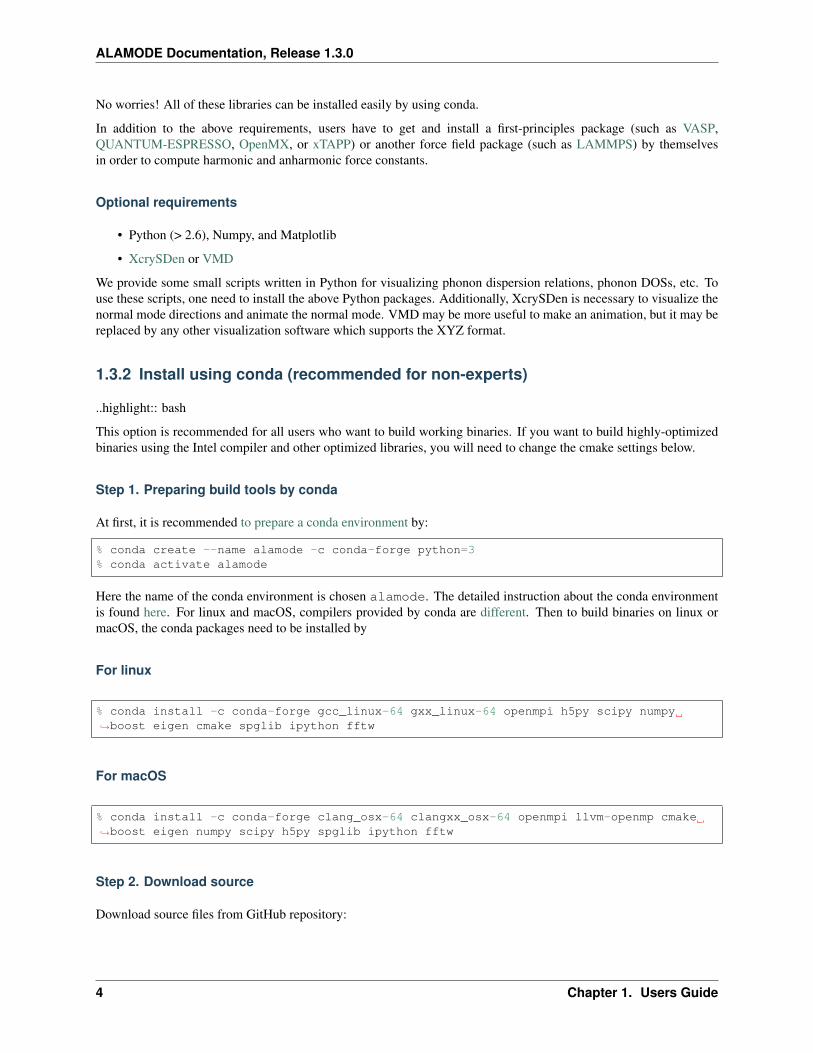
% conda install -c conda-forge gcc_linux-64 gxx_linux-64 openmpi h5py scipy numpy→˓boost eigen cmake spglib ipython fftw
For macOS
% conda install -c conda-forge clang_osx-64 clangxx_osx-64 openmpi llvm-openmp cmake→˓boost eigen numpy scipy h5py spglib ipython fftw
Step 2. Download source
Download source files from GitHub repository:
4 Chapter 1. Users Guide

ALAMODE Documentation, Release 1.3.0
% git clone https://github.com/ttadano/alamode.git% cd alamode% git checkout develop
If git command doesn’t exist in your system, it is also obtained from conda by conda install git. The directorystructure supposed in this document is shown as below:
$HOMEalamode
CMakeLists.txtalm
CMakeLists.txtanphon
CMakeLists.txtdocsexampleexternalincludetools
CMakeLists.txt
$CONDA_PREFIX/include$CONDA_PREFIX/include/eigen3$CONDA_PREFIX/lib...
The meaning of each subdirectory is as follows:
• alm/ : Source files of alm (force constant calculator)
• anphon/ : Source files of anphon (anharmonic phonon calculator)
• docs/ : Source files for making documents
• example/ : Example files
• external/ : Third-party include files
• include/ : Commonly-used include files
• tools/ : Small auxiliary programs and scripts
Step 3. Build by CMake
If you want to bulid all binaries (alm, anphon, and the others), please use CMakeLists.txt in the $HOME/alamode directory.
% pwd
* $HOME/alamode% mkdir _build; cd _build% cmake -DUSE_MKL_FFT=no ..
Please make sure that cmake detected the C++ compiler correctly. If the automatic detection fails, you can specify thecompilers by using the -DCMAKE_C_COMPILER and -DCMAKE_CXX_COMPILER options. If $CC and $CXXvariables are not set properly, you may need to conda deactivate once and conda activate alamodeagain.
After the cmake configuration finishes, build the binaries by
1.3. Installation 5

ALAMODE Documentation, Release 1.3.0
% make -j
It will create all binaries in alm/, anphon/, and tools/ subdirectories under the current directory (_build). You canspecify the binary to build, for example, as
% make alm -j
Note: If the build of alm fails due to an error related to spglib, e.g., cannot find -lsymspg, please add the-DSPGLIB_ROOT option as
% cmake -DUSE_MKL_FFT=no -DSPGLIB_ROOT=$CONDA_PREFIX ..
Also, when using the binaries, it may be necessary to set $LD_LIBRARY_PATH as
% export LD_LIBRARY_PATH=$CONDA_PREFIX/lib:$CONDA_PREFIX/lib64:$LD_LIBRARY_PATH
1.3.3 Install using native environment (optional for experts)
If you are familier with unix OS and you want to use the Intel compiler, please follow the instruction below. Here, theIntel C++ compiler and the Intel MKL, including the FFTW3 wrapper, will be used for the demonstration.
Step 1. Install all required libraries
Boost C++ and Eigen3 libraries (header files only)
(If boost and Eigen3 are already installed in your system, please skip this.)
Some header files of Boost C++ and Eigen3 libraries are necessary to build ALAMODE binaries. Here, we installheader files of these libraries in $(HOME)/include. You can skip this part if these libraries are already installed onyour system.
To install the Boost C++ library, please download a source file from the webpage and unpack the file. Then, copy the‘boost’ subdirectory to $(HOME)/include. This can be done as follows:
% cd% mkdir etc; cd etc(Download a source file and mv it to ~/etc)% tar xvf boost_x_yy_z.tar.bz2% cd ../% mkdir include; cd include% ln -s ../etc/boost_x_yy_z/boost .
In this example, we place the boost files in $(HOME)/etc and create a symbolic link to the $(HOME)/boost_x_yy_z/boost in $(HOME)/include. Instead of installing from source, you can install the Boostlibrary with Homebrew on macOS and apt-get or yum command on unix..
In the same way, please install the Eigen3 include files as follows:
% cd% mkdir etc; cd etc(Download a source file and mv it to ~/etc)% tar xvf eigen-eigen-*.tar.bz2 (* is an array of letters and digits)
(continues on next page)
6 Chapter 1. Users Guide
ALAMODE Documentation, Release 1.3.0
(continued from previous page)
% cd ../% cd include% ln -s ../etc/eigen-eigen-*/Eigen .
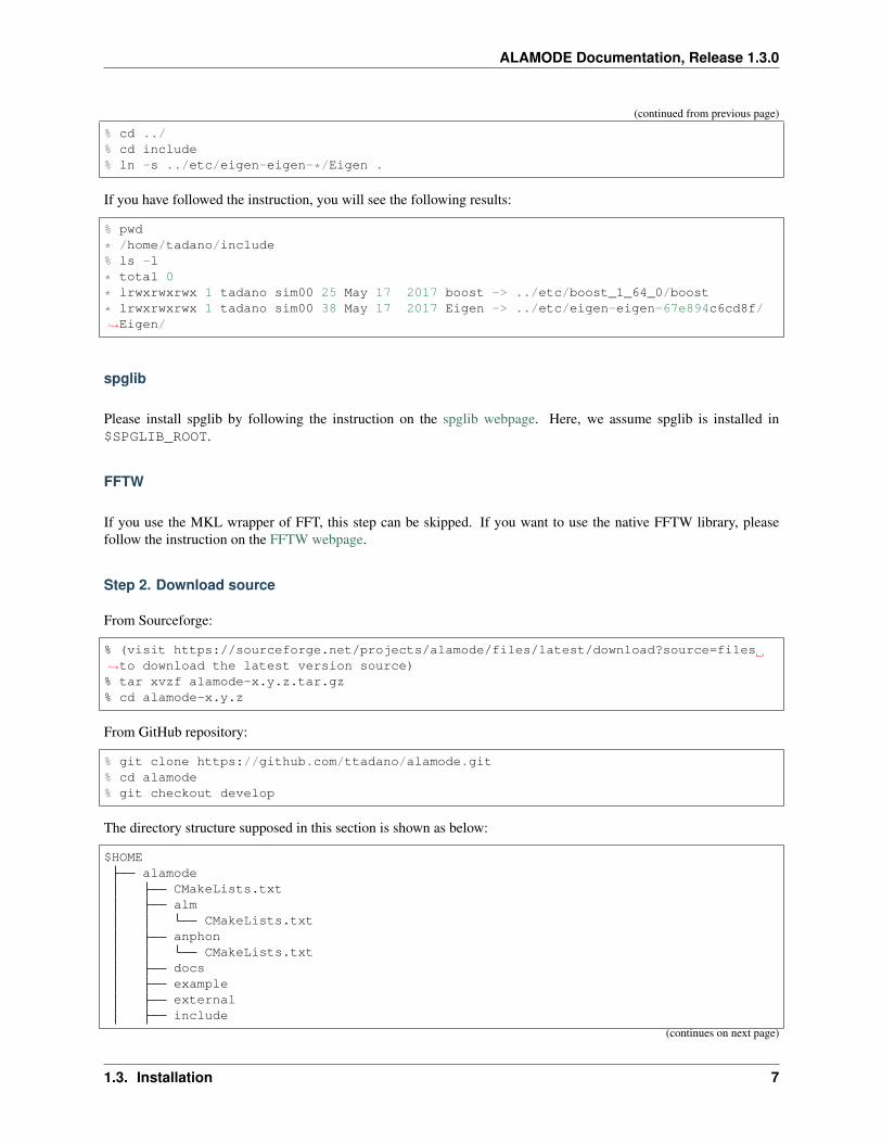
If you have followed the instruction, you will see the following results:
% pwd
* /home/tadano/include% ls -l
* total 0
* lrwxrwxrwx 1 tadano sim00 25 May 17 2017 boost -> ../etc/boost_1_64_0/boost
* lrwxrwxrwx 1 tadano sim00 38 May 17 2017 Eigen -> ../etc/eigen-eigen-67e894c6cd8f/→˓Eigen/
spglib
Please install spglib by following the instruction on the spglib webpage. Here, we assume spglib is installed in$SPGLIB_ROOT.
FFTW
If you use the MKL wrapper of FFT, this step can be skipped. If you want to use the native FFTW library, pleasefollow the instruction on the FFTW webpage.
Step 2. Download source
From Sourceforge:
% (visit https://sourceforge.net/projects/alamode/files/latest/download?source=files→˓to download the latest version source)% tar xvzf alamode-x.y.z.tar.gz% cd alamode-x.y.z
From GitHub repository:
% git clone https://github.com/ttadano/alamode.git% cd alamode% git checkout develop
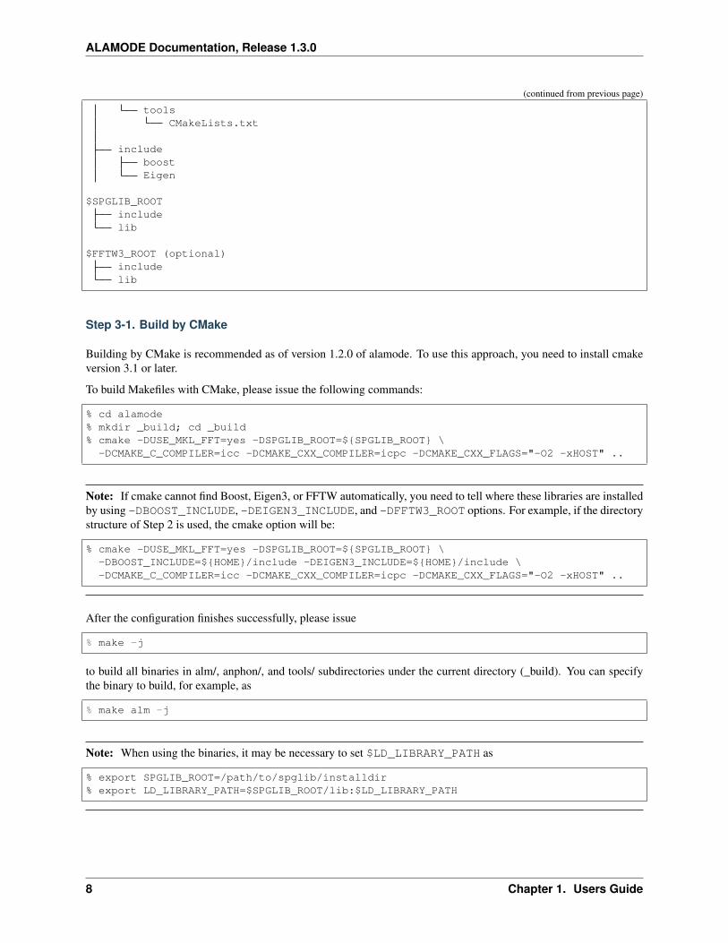
The directory structure supposed in this section is shown as below:
$HOMEalamode
CMakeLists.txtalm
CMakeLists.txtanphon
CMakeLists.txtdocsexampleexternalinclude
(continues on next page)
1.3. Installation 7
ALAMODE Documentation, Release 1.3.0
(continued from previous page)
toolsCMakeLists.txt
includeboostEigen
$SPGLIB_ROOTincludelib
$FFTW3_ROOT (optional)includelib
Step 3-1. Build by CMake
Building by CMake is recommended as of version 1.2.0 of alamode. To use this approach, you need to install cmakeversion 3.1 or later.
To build Makefiles with CMake, please issue the following commands:
% cd alamode% mkdir _build; cd _build% cmake -DUSE_MKL_FFT=yes -DSPGLIB_ROOT=$SPGLIB_ROOT \
-DCMAKE_C_COMPILER=icc -DCMAKE_CXX_COMPILER=icpc -DCMAKE_CXX_FLAGS="-O2 -xHOST" ..
Note: If cmake cannot find Boost, Eigen3, or FFTW automatically, you need to tell where these libraries are installedby using -DBOOST_INCLUDE, -DEIGEN3_INCLUDE, and -DFFTW3_ROOT options. For example, if the directorystructure of Step 2 is used, the cmake option will be:
% cmake -DUSE_MKL_FFT=yes -DSPGLIB_ROOT=$SPGLIB_ROOT \-DBOOST_INCLUDE=$HOME/include -DEIGEN3_INCLUDE=$HOME/include \-DCMAKE_C_COMPILER=icc -DCMAKE_CXX_COMPILER=icpc -DCMAKE_CXX_FLAGS="-O2 -xHOST" ..
After the configuration finishes successfully, please issue
% make -j
to build all binaries in alm/, anphon/, and tools/ subdirectories under the current directory (_build). You can specifythe binary to build, for example, as
% make alm -j
Note: When using the binaries, it may be necessary to set $LD_LIBRARY_PATH as
% export SPGLIB_ROOT=/path/to/spglib/installdir% export LD_LIBRARY_PATH=$SPGLIB_ROOT/lib:$LD_LIBRARY_PATH
8 Chapter 1. Users Guide

ALAMODE Documentation, Release 1.3.0
Step 3-2. Build by Makefile
Instead of using CMake, you can build each binary of ALAMODE by using the Makefile.linux,osx,...
In directories alm/, anphon/, and tools, we provide sample Makefiles for Linux (Intel compiler) and Mac OSX(gcc, clang). Please copy either of them, edit the options appropriately, and issue make command as follows:
% export SPGLIB_ROOT=/path/to/spglib/installdir
% cd alm/% cp Makefile.linux Makefile(Edit Makefile here)% make -j
% cd ../anphon/% cp Makefile.linux Makefile(Edit Makefile here)% make -j
% cd ../tools/% cp Makefile.linux Makefile(Edit Makefile here)% make -j
An example of the Makefiles is shown below:
Listing 1: ALM Makefile.linux
1 CXX = icpc2 CXXFLAGS = -O2 -xHOST -qopenmp -std=c++113 #CXXFLAGS = -O2 -xHOST -qopenmp -std=c++11 -D_HDF54 INCLUDE = -I../include -I$(HOME)/include -I$(SPGLIB_ROOT)/include5 #INCLUDE = -I../include -I$(HOME)/include -I$(SPGLIB_ROOT)/include -I$(HDF5_ROOT)/
→˓include6
7 CXXL = $CXX8 LDFLAGS = -mkl -L$(SPGLIB_ROOT)/lib -lsymspg9 #LDFLAGS = -mkl -L$(SPGLIB_ROOT)/lib -lsymspg -L$(HDF5_ROOT)/lib -lhdf5_cpp -lhdf5
The default options are expected to work with modern Intel compilers.
Note: When using the binaries, it may be necessary to set $LD_LIBRARY_PATH as
% export SPGLIB_ROOT=/path/to/spglib/installdir% export LD_LIBRARY_PATH=$SPGLIB_ROOT/lib:$LD_LIBRARY_PATH
1.4 Running ALAMODE
1.4.1 Program alm
Program alm estimates harmonic and anharmonic interatomic force constants (IFCs) based on the supercell approach.
1. Perform usual SCF calculations for a primitive cell
1.4. Running ALAMODE 9

ALAMODE Documentation, Release 1.3.0
Before performing phonon calculations, one needs to perform usual self-consistent field calculations andcheck the convergence with respect to the cutoff energy and the 𝑘 point density. After that, please optimizethe internal coordinate so that the atomic forces are negligibly small. Optimization of cell parameters mayalso be necessary, but please note that phonon properties are relatively sensitive to the cell parameters inpolar materials such as perovskites.
2. Decide the size of supercell
Next, please decide the size of a supercell. Here, one may use a conventional cell. When the primitivecell is fairly large (𝑎 ∼ 10 Å), one may proceed using the primitive cell.
3. Prepare an input file for alm
Please make an input file for alm, say alm.in, which should contain &general, &interaction,&cutoff, and &position entries. For details of available input variables, please refer to here. Oncethe input file is properly prepared with MODE = suggest, necessary displacement patterns can be gen-erated by executing alm as follows:
$ alm alm.in > alm.log
This produces the following files containing the pattern of atomic displacements.
• PREFIX.HARMONIC_pattern
• PREFIX.ANHARM?_pattern (If NORDER > 1)
In pattern files, all necessary displacement patterns are given in Cartesian coordinates.
Note: Pattern files just indicate the direction of displacements. The magnitude of displacements shouldbe specified by each user. (∆𝑢 ∼ 0.01 Å is usual for calculating harmonic force constants.)
4. Perform SCF calculations to generate displacement-force data set
Then, please prepare necessary input files for a DFT engine (or a classical force field engine) and calculateatomic forces for each displaced configuration. Once the atomic forces are calculated for all configura-tions, please collect the atomic displacements and atomic forces to separate files, say disp_all.dat andforce_all.dat, in Rydberg atomic units. The detail of the file format is described on this page.
Note: We provide some auxiliary Python scripts to expedite the above procedure for VASP, QuantumESPRESSO, and xTAPP users. The script files can be found in the tools/ directory. We are willing tosupport other software if necessary.
5. Estimate IFCs by linear regression
In order to perform a fitting, please change the variable MODE of the input file alm.in to MODE =optimize. In addition please add the &optimize entry with appropriate DFSET. Then, IFCs canbe estimated by executing
$ alm alm.in > alm.log
which makes the following two files in the working directory.
• PREFIX.fcs : The list of force constants
• PREFIX.xml : XML file containing necessary information for subsequent phonon calculations
10 Chapter 1. Users Guide
ALAMODE Documentation, Release 1.3.0
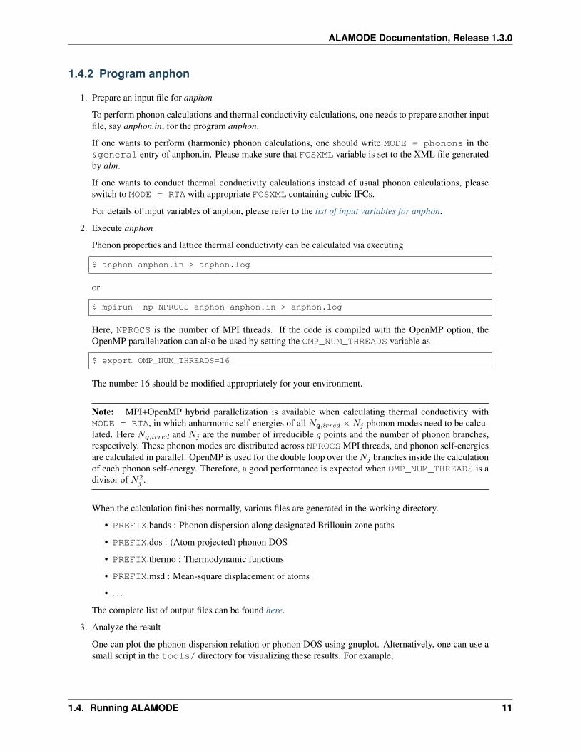
1.4.2 Program anphon
1. Prepare an input file for anphon
To perform phonon calculations and thermal conductivity calculations, one needs to prepare another inputfile, say anphon.in, for the program anphon.
If one wants to perform (harmonic) phonon calculations, one should write MODE = phonons in the&general entry of anphon.in. Please make sure that FCSXML variable is set to the XML file generatedby alm.
If one wants to conduct thermal conductivity calculations instead of usual phonon calculations, pleaseswitch to MODE = RTA with appropriate FCSXML containing cubic IFCs.
For details of input variables of anphon, please refer to the list of input variables for anphon.
2. Execute anphon
Phonon properties and lattice thermal conductivity can be calculated via executing
$ anphon anphon.in > anphon.log
or
$ mpirun -np NPROCS anphon anphon.in > anphon.log
Here, NPROCS is the number of MPI threads. If the code is compiled with the OpenMP option, theOpenMP parallelization can also be used by setting the OMP_NUM_THREADS variable as
$ export OMP_NUM_THREADS=16
The number 16 should be modified appropriately for your environment.
Note: MPI+OpenMP hybrid parallelization is available when calculating thermal conductivity withMODE = RTA, in which anharmonic self-energies of all 𝑁𝑞,𝑖𝑟𝑟𝑒𝑑 ×𝑁𝑗 phonon modes need to be calcu-lated. Here 𝑁𝑞,𝑖𝑟𝑟𝑒𝑑 and 𝑁𝑗 are the number of irreducible 𝑞 points and the number of phonon branches,respectively. These phonon modes are distributed across NPROCS MPI threads, and phonon self-energiesare calculated in parallel. OpenMP is used for the double loop over the 𝑁𝑗 branches inside the calculationof each phonon self-energy. Therefore, a good performance is expected when OMP_NUM_THREADS is adivisor of 𝑁2
𝑗 .
When the calculation finishes normally, various files are generated in the working directory.
• PREFIX.bands : Phonon dispersion along designated Brillouin zone paths
• PREFIX.dos : (Atom projected) phonon DOS
• PREFIX.thermo : Thermodynamic functions
• PREFIX.msd : Mean-square displacement of atoms
• . . .
The complete list of output files can be found here.
3. Analyze the result
One can plot the phonon dispersion relation or phonon DOS using gnuplot. Alternatively, one can use asmall script in the tools/ directory for visualizing these results. For example,
1.4. Running ALAMODE 11
ALAMODE Documentation, Release 1.3.0
$ plotband.py target.bands
shows the phonon dispersion relation. Available command line options can be displayed by
$ plotband.py -h
We also provide a similar script for phonon DOS. Another script analyze_phonons.pymay be usefulto analyze the result of thermal conductivity calculations. For example, phonon lifetimes and mean-free-path at 300 K can be extracted by
$ analyze_phonons.py --calc tau --temp 300 target.result
It can also estimate a cumulative thermal conductivity by
$ analyze_phonons.py --calc cumulative --temp 300 --direction 1 target.result
For details, see the tutorial.
1.5 ALM: Force constant calculator
1.5.1 ALM: Input files
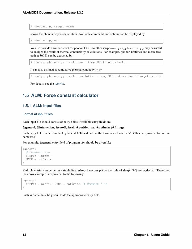
Format of input files
Each input file should consist of entry fields. Available entry fields are
&general, &interaction, &cutoff, &cell, &position, and &optimize (&fitting).
Each entry field starts from the key label &field and ends at the terminate character “/”. (This is equivalent to Fortrannamelist.)
For example, &general entry field of program alm should be given like
&general# Comment linePREFIX = prefixMODE = optimize
/
Multiple entries can be put in a single line. Also, characters put on the right of sharp (“#”) are neglected. Therefore,the above example is equivalent to the following:
&generalPREFIX = prefix; MODE = optimize # Comment line
/
Each variable must be given inside the appropriate entry field.
12 Chapter 1. Users Guide
ALAMODE Documentation, Release 1.3.0
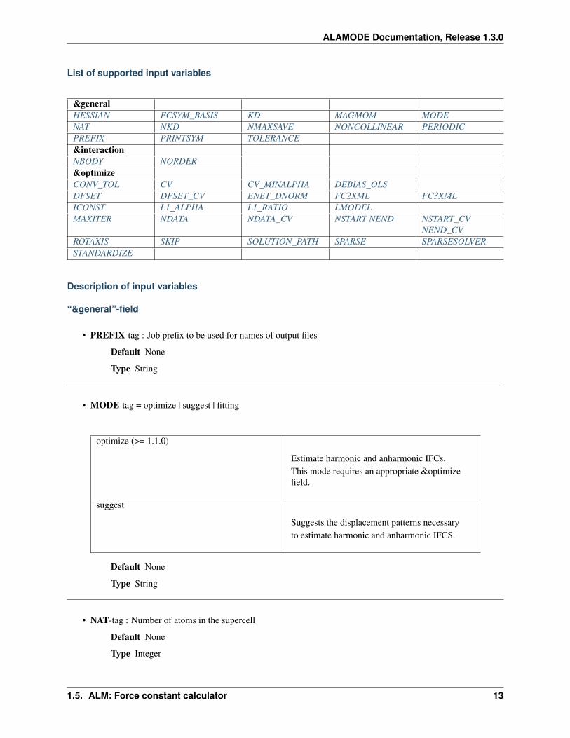
List of supported input variables
&generalHESSIAN FCSYM_BASIS KD MAGMOM MODENAT NKD NMAXSAVE NONCOLLINEAR PERIODICPREFIX PRINTSYM TOLERANCE&interactionNBODY NORDER&optimizeCONV_TOL CV CV_MINALPHA DEBIAS_OLSDFSET DFSET_CV ENET_DNORM FC2XML FC3XMLICONST L1_ALPHA L1_RATIO LMODELMAXITER NDATA NDATA_CV NSTART NEND NSTART_CV
NEND_CVROTAXIS SKIP SOLUTION_PATH SPARSE SPARSESOLVERSTANDARDIZE
Description of input variables
“&general”-field
• PREFIX-tag : Job prefix to be used for names of output files
Default None
Type String
• MODE-tag = optimize | suggest | fitting
optimize (>= 1.1.0)
Estimate harmonic and anharmonic IFCs.This mode requires an appropriate &optimizefield.
suggest
Suggests the displacement patterns necessaryto estimate harmonic and anharmonic IFCS.
Default None
Type String
• NAT-tag : Number of atoms in the supercell
Default None
Type Integer
1.5. ALM: Force constant calculator 13

ALAMODE Documentation, Release 1.3.0
• NKD-tag : Number of atomic species
Default None
Type Integer
• KD-tag = Name[1], . . . , Name[NKD]
Default None
Type Array of strings
Example In the case of GaAs with NKD = 2, it should be KD = Ga As.
• TOLERANCE-tag : Tolerance for finding symmetry operations
Default 1.0e-3
Type Double
• PRINTSYM-tag = 0 | 1
0 Symmetry operations won’t be saved in “SYMM_INFO”1 Symmetry operations will be saved in “SYMM_INFO”
Default 0
type Integer
• FCSYM_BASIS-tag = Cartesian | Lattice
Cartesian, C Symmetry reduction of force constant is performed in the Cartesian basisLattice, L Symmetry reduction of force constant is performed in the 𝑎1,𝑎2,𝑎3 basis
Default Lattice
type String
Description The calculation results should not depend on the choice of FCSYM_BASISwhenLMODEL = ols. For other regression methods (enet, adaptive LASSO), an optimalvalue of the L1_ALPHA changes when you change the FCSYM_BASIS option.
In some cases, FCSYM_BASIS = Lattice is more stable and efficient. In particular,we recommend setting FCSYM_BASIS = Lattice for hexagonal systems. If a calcu-lation with FCSYM_BASIS = Lattice is slow, please switch to FCSYM_BASIS =Cartesian.
For more details about the symmetry reduction of force constants, please see here.
14 Chapter 1. Users Guide
ALAMODE Documentation, Release 1.3.0
Important: When FCSYM_BASIS = Lattice, the basis of force constants saved in PREFIX.fcsbecomes the 𝑎1,𝑎2,𝑎3 basis. Hence, to compare the values of force constants saved in PREFIX.fcs,you will have to change their basis to the Cartesian basis manually. The basis of force constants saved inPREFIX.xml is Cartesian irrespective of the FCSYM_BASIS value.
Also, imposing the constraints for rotational invariance with FCSYM_BASIS = Lattice is notsupported. Therefore, if you want to apply the constraints for rotational invariance, please useFCSYM_BASIS = Cartesian.
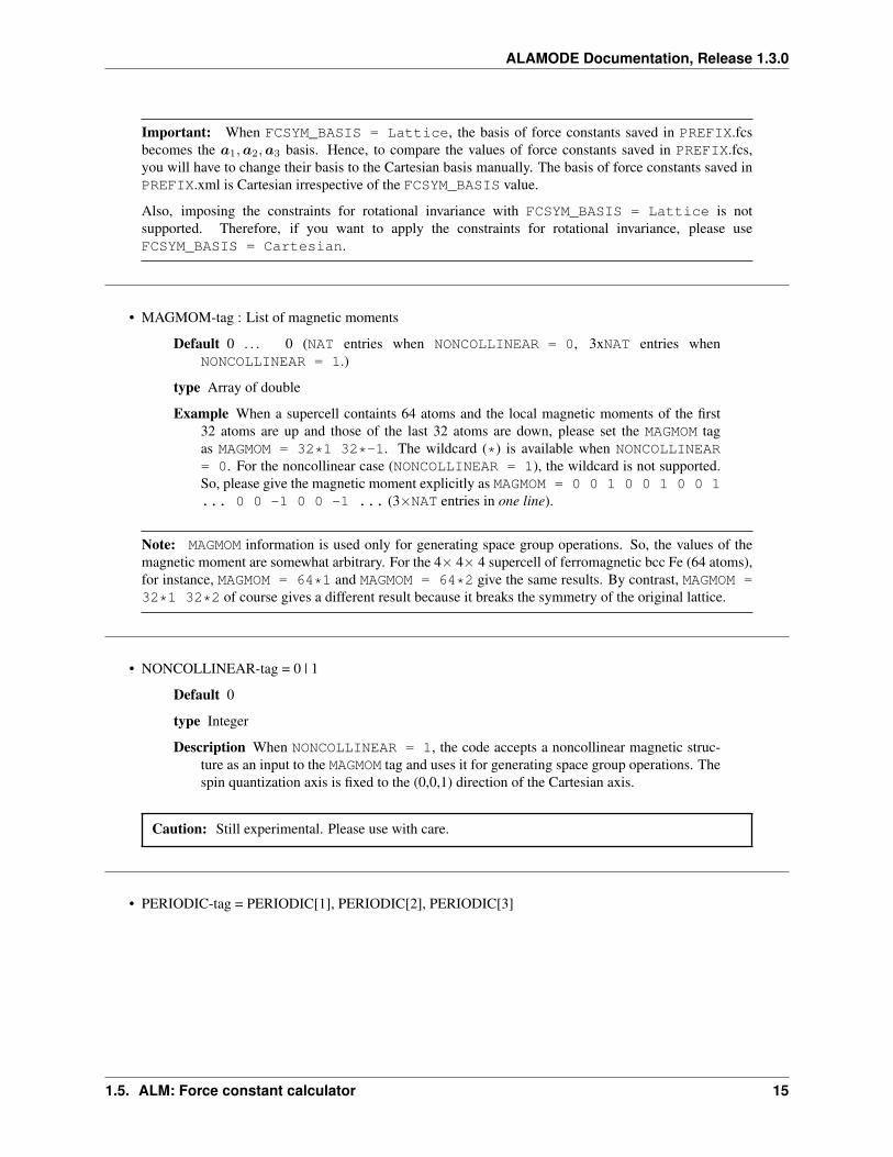
• MAGMOM-tag : List of magnetic moments
Default 0 . . . 0 (NAT entries when NONCOLLINEAR = 0, 3xNAT entries whenNONCOLLINEAR = 1.)
type Array of double
Example When a supercell containts 64 atoms and the local magnetic moments of the first32 atoms are up and those of the last 32 atoms are down, please set the MAGMOM tagas MAGMOM = 32*1 32*-1. The wildcard (*) is available when NONCOLLINEAR= 0. For the noncollinear case (NONCOLLINEAR = 1), the wildcard is not supported.So, please give the magnetic moment explicitly as MAGMOM = 0 0 1 0 0 1 0 0 1... 0 0 -1 0 0 -1 ... (3×NAT entries in one line).
Note: MAGMOM information is used only for generating space group operations. So, the values of themagnetic moment are somewhat arbitrary. For the 4× 4× 4 supercell of ferromagnetic bcc Fe (64 atoms),for instance, MAGMOM = 64*1 and MAGMOM = 64*2 give the same results. By contrast, MAGMOM =32*1 32*2 of course gives a different result because it breaks the symmetry of the original lattice.
• NONCOLLINEAR-tag = 0 | 1
Default 0
type Integer
Description When NONCOLLINEAR = 1, the code accepts a noncollinear magnetic struc-ture as an input to the MAGMOM tag and uses it for generating space group operations. Thespin quantization axis is fixed to the (0,0,1) direction of the Cartesian axis.
Caution: Still experimental. Please use with care.
• PERIODIC-tag = PERIODIC[1], PERIODIC[2], PERIODIC[3]
1.5. ALM: Force constant calculator 15

ALAMODE Documentation, Release 1.3.0
0
Do not consider periodic boundary conditionswhensearching for interacting atoms.
1
Consider periodic boundary conditions whensearching for interacting atoms.
Default 1 1 1
type Array of integers
Description This tag is useful for generating interacting atoms in low dimensional systems.When PERIODIC[i] is zero, periodic boundary condition is turned off along the direc-tion of the lattice vector 𝑎𝑖.
• NMAXSAVE-tag : The maximum order of anharmonic force constants printed out in PREFIX.xml
Default min(5, NORDER)
Type Integer
Example If your model includes anharmonic terms up to the sixth-order (NORDER = 5), butyou want to avoid printing out the fifth-order and sixth-order IFCs in PREFIX.xml, pleaseset NMAXSAVE = 3.
• HESSIAN-tag = 0 | 1
0 Do not save the Hessian matrix1 Save the entire Hessian matrix of the supercell as PREFIX.hessian.
Default 0
type Integer
“&interaction”-field
• NORDER-tag : The order of force constants to be calculated. Anharmonic terms up to (𝑚 + 1)th order will beconsidered with NORDER = 𝑚.
Default None
Type Integer
Example NORDER = 1 for calculate harmonic terms only, NORDER = 2 to include cubicterms as well, and so on.
• NBODY-tag : Entry for excluding multiple-body interactions from anharmonic force constants
16 Chapter 1. Users Guide

ALAMODE Documentation, Release 1.3.0
Default NBODY = [2, 3, 4, . . . , NORDER + 1]
Type Array of integers
Description This tag may be useful for excluding multi-body clusters which are supposedlyless important. For example, a set of fourth-order IFCs Φ𝑖𝑗𝑘𝑙, where 𝑖, 𝑗, 𝑘, and 𝑙 labelatoms in the supercell, can be categorized into four different subsets; on-site, two-body,three-body, and four-body terms. Neglecting the Cartesian coordinates of IFCs for sim-plicity, each subset contains the IFC elements shown as follows:
on-site
Φ𝑖𝑖𝑖𝑖
two-body
Φ𝑖𝑖𝑗𝑗, Φ𝑖𝑖𝑖𝑗 (𝑖 = 𝑗)
three-body
Φ𝑖𝑖𝑗𝑘 (𝑖 = 𝑗, 𝑖 = 𝑘, 𝑗 = 𝑘)
four-body
Φ𝑖𝑗𝑘𝑙 (all subscripts are different fromeach other)
Since the four-body clusters are expected to be less important than the three-body and less-body clusters, you may want to exclude the four-body terms from the Taylor expansionpotential because the number of such terms is huge. This can be done by setting theNBODY tag as NBODY = 2 3 3 together with NORDER = 3.
More examples NORDER = 2; NBODY = 2 2 includes harmonic and cubic IFCs but ex-cludes three-body clusters from the cubic terms.
NORDER = 5; NBODY = 2 3 3 2 2 includes anharmonic terms up to the sixth-order, where the four-body clusters are excluded from the fourth-order IFCs, and the multi(≥ 3)-body clusters are excluded from the fifth- and sixth-order IFCs.
“&cutoff”-field
In this entry field, one needs to specify cutoff radii of interaction for each order in units of bohr. In the currentimplementation, cutoff radii should be defined for every possible pair of atomic elements. For example, the cutoffentry for a harmonic calculation (NORDER = 1) of Si (NKD = 1) should be like
&cutoffSi-Si 10.0
/
This means that the cutoff radius of 10 𝑎0 is used for harmonic Si-Si terms. Please note that the first column shouldbe two character strings, which are contained in the KD-tag, connected by a hyphen (’-’).
When one wants to consider cubic terms (NORDER = 2), please specify the cutoff radius for cubic terms in the thirdcolumn as the following:
1.5. ALM: Force constant calculator 17
ALAMODE Documentation, Release 1.3.0
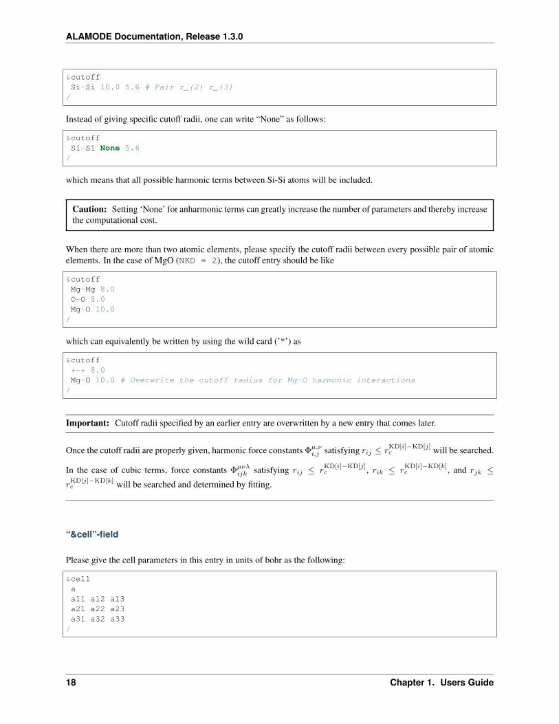
&cutoffSi-Si 10.0 5.6 # Pair r_2 r_3
/
Instead of giving specific cutoff radii, one can write “None” as follows:
&cutoffSi-Si None 5.6
/
which means that all possible harmonic terms between Si-Si atoms will be included.
Caution: Setting ‘None’ for anharmonic terms can greatly increase the number of parameters and thereby increasethe computational cost.
When there are more than two atomic elements, please specify the cutoff radii between every possible pair of atomicelements. In the case of MgO (NKD = 2), the cutoff entry should be like
&cutoffMg-Mg 8.0O-O 8.0Mg-O 10.0
/
which can equivalently be written by using the wild card (’*’) as
&cutoff
*-* 8.0Mg-O 10.0 # Overwrite the cutoff radius for Mg-O harmonic interactions
/
Important: Cutoff radii specified by an earlier entry are overwritten by a new entry that comes later.
Once the cutoff radii are properly given, harmonic force constants Φ𝜇,𝜈𝑖,𝑗 satisfying 𝑟𝑖𝑗 ≤ 𝑟
KD[𝑖]−KD[𝑗]𝑐 will be searched.
In the case of cubic terms, force constants Φ𝜇𝜈𝜆𝑖𝑗𝑘 satisfying 𝑟𝑖𝑗 ≤ 𝑟
KD[𝑖]−KD[𝑗]𝑐 , 𝑟𝑖𝑘 ≤ 𝑟
KD[𝑖]−KD[𝑘]𝑐 , and 𝑟𝑗𝑘 ≤
𝑟KD[𝑗]−KD[𝑘]𝑐 will be searched and determined by fitting.
“&cell”-field
Please give the cell parameters in this entry in units of bohr as the following:
&cellaa11 a12 a13a21 a22 a23a31 a32 a33
/
18 Chapter 1. Users Guide
ALAMODE Documentation, Release 1.3.0
The cell parameters are then given by 1 = 𝑎× (𝑎11, 𝑎12, 𝑎13), 2 = 𝑎× (𝑎21, 𝑎22, 𝑎23), and 3 = 𝑎× (𝑎31, 𝑎32, 𝑎33).
“&position”-field
In this field, one needs to specify the atomic element and fractional coordinate of atoms in the supercell. Each lineshould be
ikd xf[1] xf[2] xf[3]
where ikd is an integer specifying the atomic element (ikd = 1, . . . , NKD) and xf[i] is the fractional coordinate of anatom. There should be NAT such lines in the &position entry field.
“&optimize”-field (”&fitting”-field)
This field is necessary when MODE = optimize.
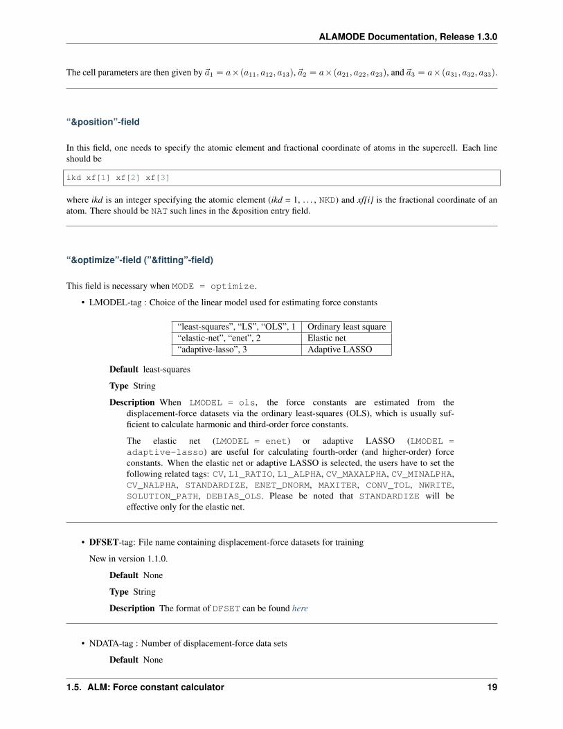
• LMODEL-tag : Choice of the linear model used for estimating force constants
“least-squares”, “LS”, “OLS”, 1 Ordinary least square“elastic-net”, “enet”, 2 Elastic net“adaptive-lasso”, 3 Adaptive LASSO
Default least-squares
Type String
Description When LMODEL = ols, the force constants are estimated from thedisplacement-force datasets via the ordinary least-squares (OLS), which is usually suf-ficient to calculate harmonic and third-order force constants.
The elastic net (LMODEL = enet) or adaptive LASSO (LMODEL =adaptive-lasso) are useful for calculating fourth-order (and higher-order) forceconstants. When the elastic net or adaptive LASSO is selected, the users have to set thefollowing related tags: CV, L1_RATIO, L1_ALPHA, CV_MAXALPHA, CV_MINALPHA,CV_NALPHA, STANDARDIZE, ENET_DNORM, MAXITER, CONV_TOL, NWRITE,SOLUTION_PATH, DEBIAS_OLS. Please be noted that STANDARDIZE will beeffective only for the elastic net.
• DFSET-tag: File name containing displacement-force datasets for training
New in version 1.1.0.
Default None
Type String
Description The format of DFSET can be found here
• NDATA-tag : Number of displacement-force data sets
Default None
1.5. ALM: Force constant calculator 19
ALAMODE Documentation, Release 1.3.0
Type Integer
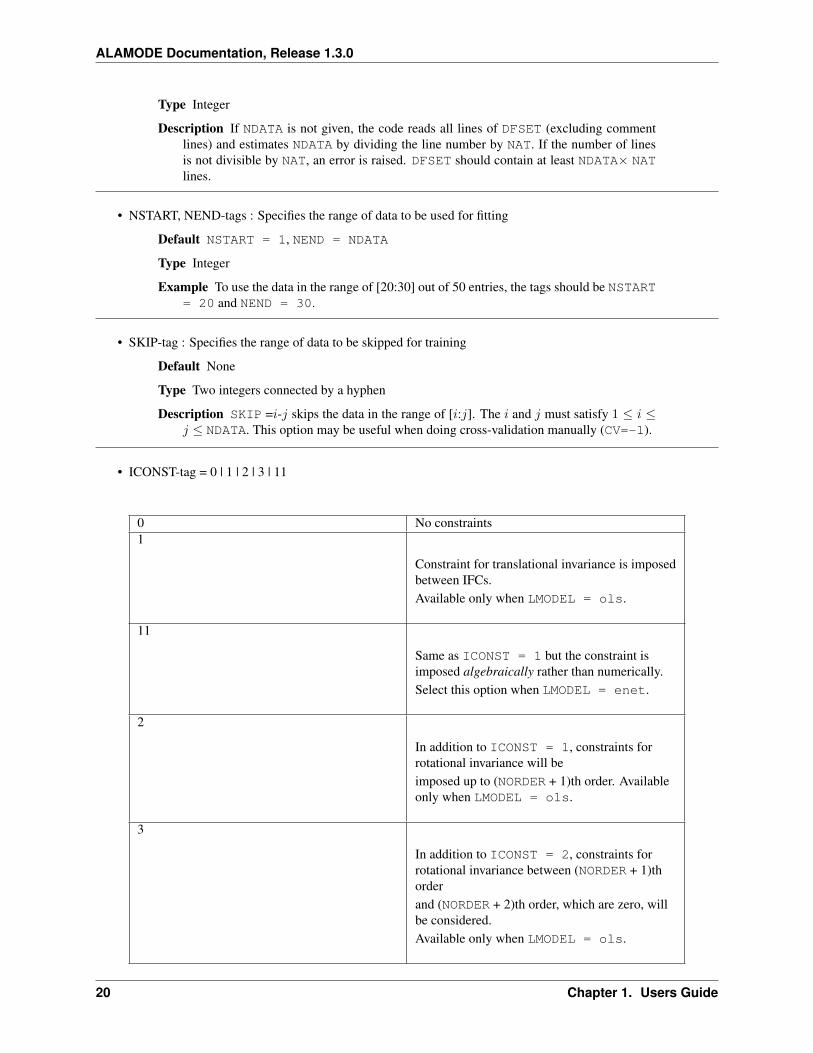
Description If NDATA is not given, the code reads all lines of DFSET (excluding commentlines) and estimates NDATA by dividing the line number by NAT. If the number of linesis not divisible by NAT, an error is raised. DFSET should contain at least NDATA× NATlines.
• NSTART, NEND-tags : Specifies the range of data to be used for fitting
Default NSTART = 1, NEND = NDATA
Type Integer
Example To use the data in the range of [20:30] out of 50 entries, the tags should be NSTART= 20 and NEND = 30.
• SKIP-tag : Specifies the range of data to be skipped for training
Default None
Type Two integers connected by a hyphen
Description SKIP =𝑖-𝑗 skips the data in the range of [𝑖:𝑗]. The 𝑖 and 𝑗 must satisfy 1 ≤ 𝑖 ≤𝑗 ≤ NDATA. This option may be useful when doing cross-validation manually (CV=-1).
• ICONST-tag = 0 | 1 | 2 | 3 | 11
0 No constraints1
Constraint for translational invariance is imposedbetween IFCs.Available only when LMODEL = ols.
11
Same as ICONST = 1 but the constraint isimposed algebraically rather than numerically.Select this option when LMODEL = enet.
2
In addition to ICONST = 1, constraints forrotational invariance will beimposed up to (NORDER + 1)th order. Availableonly when LMODEL = ols.
3
In addition to ICONST = 2, constraints forrotational invariance between (NORDER + 1)thorderand (NORDER + 2)th order, which are zero, willbe considered.Available only when LMODEL = ols.
20 Chapter 1. Users Guide
ALAMODE Documentation, Release 1.3.0
Default 11
Type Integer
Description See this page for the numerical formulae.
• ROTAXIS-tag : Rotation axis used to estimate constraints for rotational invariance. This entry is necessarywhen ICONST = 2, 3.
Default None
Type String
Example When one wants to consider the rotational invariance around the 𝑥-axis, one shouldgive ROTAXIS = x. If one needs additional constraints for the rotation around the 𝑦-axis, ROTAXIS should be ROTAXIS = xy.
• FC2XML-tag : XML file to which the harmonic terms are fixed upon fitting
Default None
Type String
Description When FC2XML-tag is given, harmonic force constants are fixed to the valuesstored in the FC2XML file. This may be useful for optimizing cubic and higher-order termswithout changing the harmonic terms. Please make sure that the number of harmonicterms in the new computational condition is the same as that in the FC2XML file.
Important: The FCSYM_BASIS option must be the same as the one used when creating the referenceharmonic force constant file (FC2XML). The code raises an error when they are inconsistent.
• FC3XML-tag : XML file to which the cubic terms are fixed upon fitting
Default None
Type String
Description Same as the FC2XML-tag, but FC3XML is to fix cubic force constants.
Important: The FCSYM_BASIS option must be the same as the one used when creating the referencecubic force constant file (FC3XML). The code raises an error when they are inconsistent.
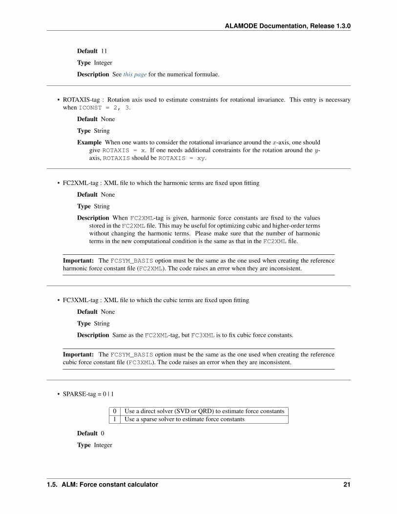
• SPARSE-tag = 0 | 1
0 Use a direct solver (SVD or QRD) to estimate force constants1 Use a sparse solver to estimate force constants
Default 0
Type Integer
1.5. ALM: Force constant calculator 21
ALAMODE Documentation, Release 1.3.0
Description When you want to calculate force constants of a large system and generate train-ing datasets by displacing only a few atoms from equilibrium positions, the resulting sens-ing matrix becomes large but sparse. For such matrices, a sparse solver is expected to bemore efficient than SVD or QRD in terms of both memory usage and computational time.When SPARSE = 1 is set, the code uses a sparse solver implemented in Eigen3 library.You can change the solver type via SPARSESOLVER. Effective when LMODEL = ols.
• SPARSESOLVER-tag : Type of the sparse solver to use
Default SimplicialLDLT
Type String
Description Currently, only the sparse solvers of Eigen3 library can be used. Available op-tions are SimplicialLDLT, SparseQR, ConjugateGradient, LeastSquaresConjugateGradi-ent, and BiCGSTAB. When an iterative algorithm (conjugate gradient) is selected, a stop-ping criterion can be specified by the CONV_TOL and MAXITER tags. Effective whenLMODEL = ols and SPARSE = 1.
See also:
Eigen documentation page: Solving Sparse Linear Systems
• MAXITER-tag : Number of maximum iterations in iterative algorithms
Default 10,000
Type Integer
Description Effective when an iterative solver is selected via SPARSESOLVER (whenLMODEL = ols) or when LMODEL = enet | adaptive-lasso.
• CONV_TOL-tag : Convergence criterion of iterative algorithms
Default 1.0e-8
Type Double
Description When LMODEL = ols and an iterative solver is selected via SPARSESOLVER,CONV_TOL value is passed to the Eigen3 function via setTolerance(). When LMODEL =enet | adaptive-lasso, the coordinate descent iteration stops at 𝑖th iteration if√
1𝑁 |Φ𝑖 −Φ𝑖−1|22 < CONV_TOL is satisfied, where 𝑁 is the length of the vector Φ.
See also:
Eigen documentation page: IterativeSolverBase
• L1_RATIO-tag : The ratio of the L1 regularization term
Default 1.0 (LASSO)
Type Double
Description The L1_RATIO changes the regularization term as L1_ALPHA × [L1_RATIO|Φ|1 + 1
2 (1-L1_RATIO) |Φ|22]. Therefore, L1_RATIO = 1 corresponds to LASSO.L1_RATIO must be 0 < L1_ratio <= 1. Effective when LMODEL = enet. Seealso here.
22 Chapter 1. Users Guide
ALAMODE Documentation, Release 1.3.0
• L1_ALPHA-tag : The coefficient of the L1 regularization term
Default 0.0
Type Double
Description This tag is used when LMODEL = enet | adaptive-lasso and CV =0. See also here.
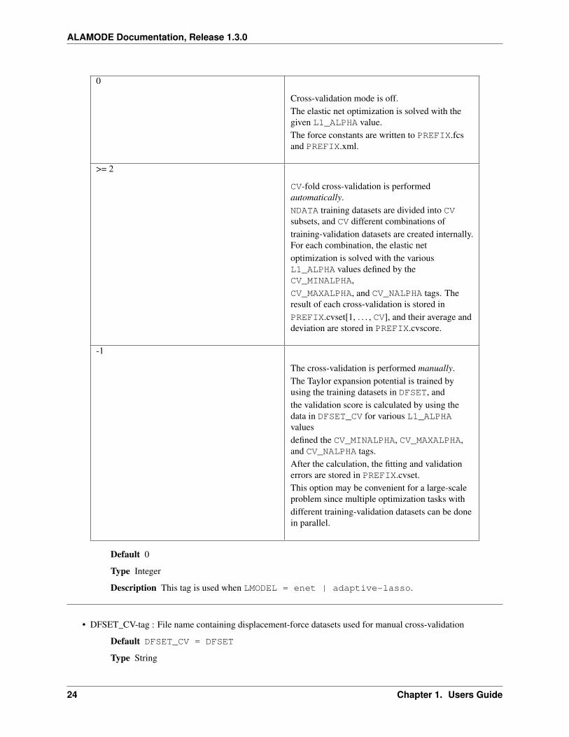
• CV-tag : Cross-validation mode for elastic net
1.5. ALM: Force constant calculator 23
ALAMODE Documentation, Release 1.3.0
0
Cross-validation mode is off.The elastic net optimization is solved with thegiven L1_ALPHA value.The force constants are written to PREFIX.fcsand PREFIX.xml.
>= 2
CV-fold cross-validation is performedautomatically.NDATA training datasets are divided into CVsubsets, and CV different combinations oftraining-validation datasets are created internally.For each combination, the elastic netoptimization is solved with the variousL1_ALPHA values defined by theCV_MINALPHA,CV_MAXALPHA, and CV_NALPHA tags. Theresult of each cross-validation is stored inPREFIX.cvset[1, . . . , CV], and their average anddeviation are stored in PREFIX.cvscore.
-1
The cross-validation is performed manually.The Taylor expansion potential is trained byusing the training datasets in DFSET, andthe validation score is calculated by using thedata in DFSET_CV for various L1_ALPHAvaluesdefined the CV_MINALPHA, CV_MAXALPHA,and CV_NALPHA tags.After the calculation, the fitting and validationerrors are stored in PREFIX.cvset.This option may be convenient for a large-scaleproblem since multiple optimization tasks withdifferent training-validation datasets can be donein parallel.
Default 0
Type Integer
Description This tag is used when LMODEL = enet | adaptive-lasso.
• DFSET_CV-tag : File name containing displacement-force datasets used for manual cross-validation
Default DFSET_CV = DFSET
Type String
24 Chapter 1. Users Guide
ALAMODE Documentation, Release 1.3.0
Description This tag is used when LMODEL = enet | adaptive-lasso and CV =-1.
• NDATA_CV-tag : Number of displacement-force validation datasets
Default None
Type Integer
Description This tag is used when LMODEL = enet | adaptive-lasso and CV =-1.
• NSTART_CV, NEND_CV-tags : Specifies the range of data to be used for validation
Default NSTART_CV = 1, NEND_CV = NDATA_CV
Type Integer
Example This tag is used when LMODEL = enet | adaptive-lasso and CV = -1.
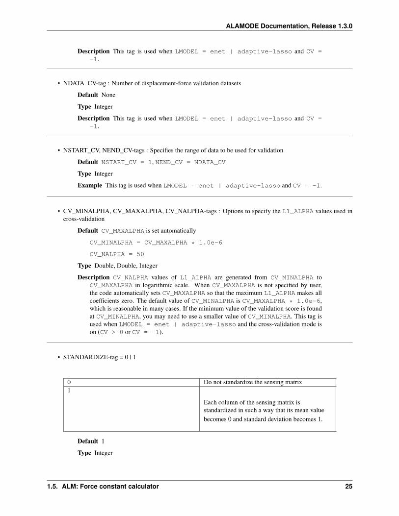
• CV_MINALPHA, CV_MAXALPHA, CV_NALPHA-tags : Options to specify the L1_ALPHA values used incross-validation
Default CV_MAXALPHA is set automatically
CV_MINALPHA = CV_MAXALPHA * 1.0e-6
CV_NALPHA = 50
Type Double, Double, Integer
Description CV_NALPHA values of L1_ALPHA are generated from CV_MINALPHA toCV_MAXALPHA in logarithmic scale. When CV_MAXALPHA is not specified by user,the code automatically sets CV_MAXALPHA so that the maximum L1_ALPHA makes allcoefficients zero. The default value of CV_MINALPHA is CV_MAXALPHA * 1.0e-6,which is reasonable in many cases. If the minimum value of the validation score is foundat CV_MINALPHA, you may need to use a smaller value of CV_MINALPHA. This tag isused when LMODEL = enet | adaptive-lasso and the cross-validation mode ison (CV > 0 or CV = -1).
• STANDARDIZE-tag = 0 | 1
0 Do not standardize the sensing matrix1
Each column of the sensing matrix isstandardized in such a way that its mean valuebecomes 0 and standard deviation becomes 1.
Default 1
Type Integer
1.5. ALM: Force constant calculator 25
ALAMODE Documentation, Release 1.3.0
Description This option influences the optimal L1_ALPHA value. So, if you change theSTANDARDIZE option, you have to rerun the cross-validation. Effective only whenLMODEL = enet.
• ENET_DNORM-tag : Normalization factor of atomic displacements
Default 1.0
Type Double
Description The normalization factor of atomic displacement 𝑢0 in units of bohr. When 𝑢0( =1) is given, the displacement data are scaled as 𝑢𝑖 → 𝑢𝑖/𝑢0 before constructing thesensing matrix. This option influences the optimal L1_ALPHA value. So, if you changethe ENET_DNORM value, you will have to rerun the cross-validation. Effective only whenLMODEL = enet and STANDARDIZE = 0.
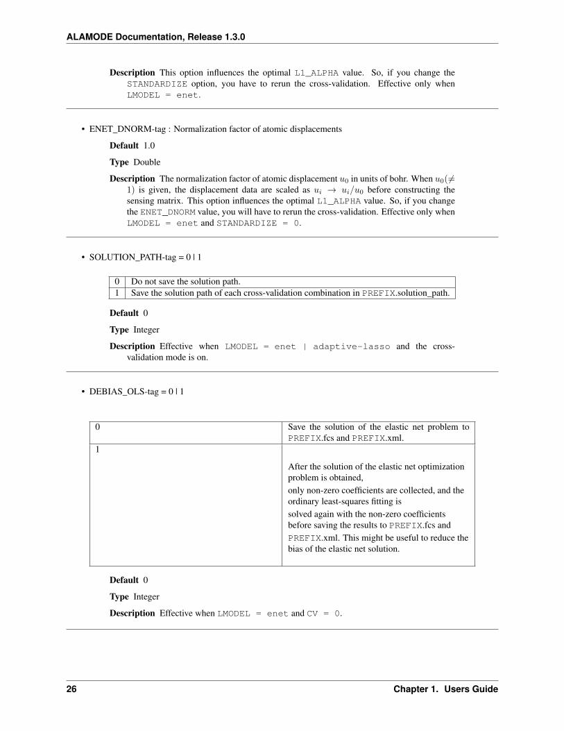
• SOLUTION_PATH-tag = 0 | 1
0 Do not save the solution path.1 Save the solution path of each cross-validation combination in PREFIX.solution_path.
Default 0
Type Integer
Description Effective when LMODEL = enet | adaptive-lasso and the cross-validation mode is on.
• DEBIAS_OLS-tag = 0 | 1
0 Save the solution of the elastic net problem toPREFIX.fcs and PREFIX.xml.
1
After the solution of the elastic net optimizationproblem is obtained,only non-zero coefficients are collected, and theordinary least-squares fitting issolved again with the non-zero coefficientsbefore saving the results to PREFIX.fcs andPREFIX.xml. This might be useful to reduce thebias of the elastic net solution.
Default 0
Type Integer
Description Effective when LMODEL = enet and CV = 0.
26 Chapter 1. Users Guide
ALAMODE Documentation, Release 1.3.0
How to make a DFSET file
Format of DFSET
The displacement-force data sets obtained by first-principles (or classical force-field) calculations have to be saved to afile, say DFSET. Then, the force constants are estimated by setting DFSET =DFSET and with MODE = optimize.
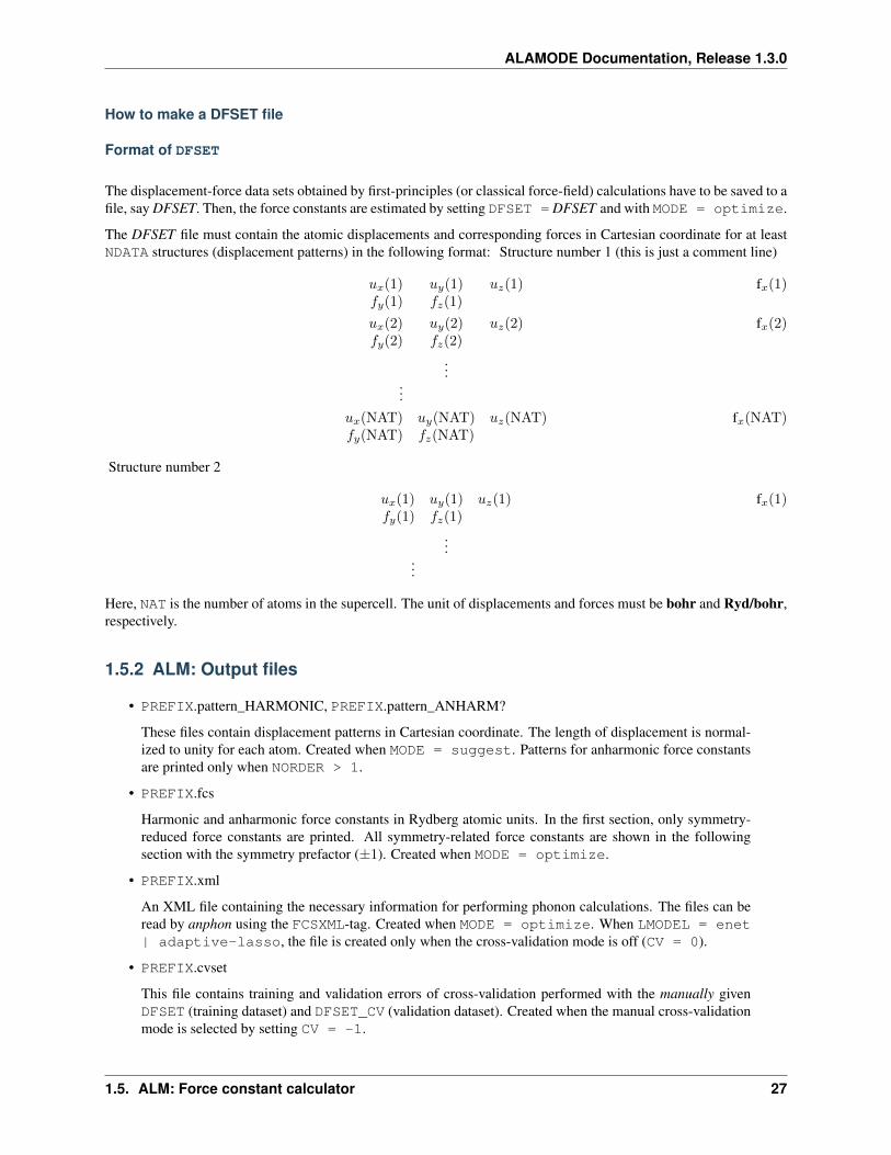
The DFSET file must contain the atomic displacements and corresponding forces in Cartesian coordinate for at leastNDATA structures (displacement patterns) in the following format: Structure number 1 (this is just a comment line)
𝑢𝑥(1) 𝑢𝑦(1) 𝑢𝑧(1) f𝑥(1)𝑓𝑦(1) 𝑓𝑧(1)
𝑢𝑥(2) 𝑢𝑦(2) 𝑢𝑧(2) f𝑥(2)𝑓𝑦(2) 𝑓𝑧(2)
......
𝑢𝑥(NAT) 𝑢𝑦(NAT) 𝑢𝑧(NAT) f𝑥(NAT)𝑓𝑦(NAT) 𝑓𝑧(NAT)
Structure number 2
𝑢𝑥(1) 𝑢𝑦(1) 𝑢𝑧(1) f𝑥(1)𝑓𝑦(1) 𝑓𝑧(1)
......
Here, NAT is the number of atoms in the supercell. The unit of displacements and forces must be bohr and Ryd/bohr,respectively.
1.5.2 ALM: Output files
• PREFIX.pattern_HARMONIC, PREFIX.pattern_ANHARM?
These files contain displacement patterns in Cartesian coordinate. The length of displacement is normal-ized to unity for each atom. Created when MODE = suggest. Patterns for anharmonic force constantsare printed only when NORDER > 1.
• PREFIX.fcs
Harmonic and anharmonic force constants in Rydberg atomic units. In the first section, only symmetry-reduced force constants are printed. All symmetry-related force constants are shown in the followingsection with the symmetry prefactor (±1). Created when MODE = optimize.
• PREFIX.xml
An XML file containing the necessary information for performing phonon calculations. The files can beread by anphon using the FCSXML-tag. Created when MODE = optimize. When LMODEL = enet| adaptive-lasso, the file is created only when the cross-validation mode is off (CV = 0).
• PREFIX.cvset
This file contains training and validation errors of cross-validation performed with the manually givenDFSET (training dataset) and DFSET_CV (validation dataset). Created when the manual cross-validationmode is selected by setting CV = -1.
1.5. ALM: Force constant calculator 27
ALAMODE Documentation, Release 1.3.0
• PREFIX.cvset[1, . . . , CV]
These files contain training and validation errors of cross-validation performed for CV subsets. Createdwhen the automatic cross-validation mode is selected by setting CV > 1.
• PREFIX.cvscore
The mean value and standard deviation of the training and validation errors are reported. Created whenthe automatic cross-validation (CV > 1) is finished.
1.5.3 ALM: Theoretical background
Interatomic force constants (IFCs)
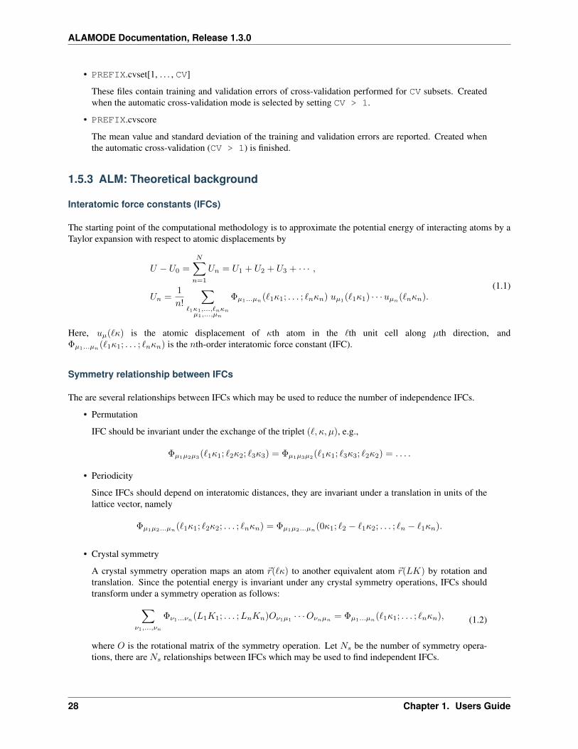
The starting point of the computational methodology is to approximate the potential energy of interacting atoms by aTaylor expansion with respect to atomic displacements by
𝑈 − 𝑈0 =
𝑁∑𝑛=1
𝑈𝑛 = 𝑈1 + 𝑈2 + 𝑈3 + · · · ,
𝑈𝑛 =1
𝑛!
∑ℓ1𝜅1,...,ℓ𝑛𝜅𝑛
𝜇1,...,𝜇𝑛
Φ𝜇1...𝜇𝑛(ℓ1𝜅1; . . . ; ℓ𝑛𝜅𝑛) 𝑢𝜇1
(ℓ1𝜅1) · · ·𝑢𝜇𝑛(ℓ𝑛𝜅𝑛).
(1.1)
Here, 𝑢𝜇(ℓ𝜅) is the atomic displacement of 𝜅th atom in the ℓth unit cell along 𝜇th direction, andΦ𝜇1...𝜇𝑛
(ℓ1𝜅1; . . . ; ℓ𝑛𝜅𝑛) is the 𝑛th-order interatomic force constant (IFC).
Symmetry relationship between IFCs
The are several relationships between IFCs which may be used to reduce the number of independence IFCs.
• Permutation
IFC should be invariant under the exchange of the triplet (ℓ, 𝜅, 𝜇), e.g.,
Φ𝜇1𝜇2𝜇3(ℓ1𝜅1; ℓ2𝜅2; ℓ3𝜅3) = Φ𝜇1𝜇3𝜇2
(ℓ1𝜅1; ℓ3𝜅3; ℓ2𝜅2) = . . . .
• Periodicity
Since IFCs should depend on interatomic distances, they are invariant under a translation in units of thelattice vector, namely
Φ𝜇1𝜇2...𝜇𝑛(ℓ1𝜅1; ℓ2𝜅2; . . . ; ℓ𝑛𝜅𝑛) = Φ𝜇1𝜇2...𝜇𝑛
(0𝜅1; ℓ2 − ℓ1𝜅2; . . . ; ℓ𝑛 − ℓ1𝜅𝑛).
• Crystal symmetry
A crystal symmetry operation maps an atom (ℓ𝜅) to another equivalent atom (𝐿𝐾) by rotation andtranslation. Since the potential energy is invariant under any crystal symmetry operations, IFCs shouldtransform under a symmetry operation as follows:∑
𝜈1,...,𝜈𝑛
Φ𝜈1...𝜈𝑛(𝐿1𝐾1; . . . ;𝐿𝑛𝐾𝑛)𝑂𝜈1𝜇1
· · ·𝑂𝜈𝑛𝜇𝑛= Φ𝜇1...𝜇𝑛
(ℓ1𝜅1; . . . ; ℓ𝑛𝜅𝑛), (1.2)
where 𝑂 is the rotational matrix of the symmetry operation. Let 𝑁𝑠 be the number of symmetry opera-tions, there are 𝑁𝑠 relationships between IFCs which may be used to find independent IFCs.
28 Chapter 1. Users Guide
ALAMODE Documentation, Release 1.3.0
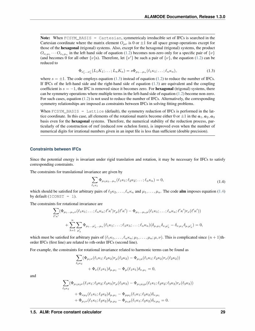
Note: When FCSYM_BASIS = Cartesian, symmetricaly irreducible set of IFCs is searched in theCartesian coordinate where the matrix element 𝑂𝜇𝜈 is 0 or ±1 for all space group operations except forthose of the hexagonal (trigonal) systems. Also, except for the hexagonal (trigonal) systems, the product𝑂𝜈1𝜇1
· · ·𝑂𝜈𝑛𝜇𝑛in the left hand side of equation (1.2) becomes non-zero only for a specific pair of 𝜈
(and becomes 0 for all other 𝜈s). Therefore, let 𝜈′ be such a pair of 𝜈, the equation (1.2) can bereduced to
Φ𝜈′1...𝜈
′𝑛(𝐿1𝐾1; . . . ;𝐿𝑛𝐾𝑛) = 𝑠Φ𝜇1...𝜇𝑛
(ℓ1𝜅1; . . . ; ℓ𝑛𝜅𝑛), (1.3)
where 𝑠 = ±1. The code employs equation (1.3) instead of equation (1.2) to reduce the number of IFCs.If IFCs of the left-hand side and the right-hand side of equation (1.3) are equivalent and the couplingcoefficient is 𝑠 = −1, the IFC is removed since it becomes zero. For hexagonal (trigonal) systems, therecan be symmetry operations where multiple terms in the left-hand side of equation (1.2) become non-zero.For such cases, equation (1.2) is not used to reduce the number of IFCs. Alternatively, the correspondingsymmetry relationships are imposed as constraints between IFCs in solving fitting problems.
When FCSYM_BASIS = Lattice (default), the symmetry reduction of IFCs is performed in the lat-tice coordinate. In this case, all elements of the rotational matrix become either 0 or ±1 in the 𝑎1,𝑎2,𝑎3
basis even for the hexagonal systems. Therefore, the numerical stability of the reduction process, par-ticularly of the construction of rref (reduced row echelon form), is improved even when the number ofnumerical digits for irrational numbers given in an input file is less than sufficient (double precision).
Constraints between IFCs
Since the potential energy is invariant under rigid translation and rotation, it may be necessary for IFCs to satisfycorresponding constraints.
The constraints for translational invariance are given by∑ℓ1𝜅1
Φ𝜇1𝜇2...𝜇𝑛(ℓ1𝜅1; ℓ2𝜅2; . . . ; ℓ𝑛𝜅𝑛) = 0, (1.4)
which should be satisfied for arbitrary pairs of ℓ2𝜅2, . . . , ℓ𝑛𝜅𝑛 and 𝜇1, . . . , 𝜇𝑛. The code alm imposes equation (1.4)by default (ICONST = 1).
The constraints for rotational invariance are∑ℓ′𝜅′
(Φ𝜇1...𝜇𝑛𝜈(ℓ1𝜅1; . . . ; ℓ𝑛𝜅𝑛; ℓ′𝜅′)𝑟𝜇(ℓ′𝜅′) − Φ𝜇1...𝜇𝑛𝜇(ℓ1𝜅1; . . . ; ℓ𝑛𝜅𝑛; ℓ′𝜅′)𝑟𝜈(ℓ′𝜅′))
+
𝑛∑𝜆=1
∑𝜇′𝜆
Φ𝜇1...𝜇′𝜆...𝜇𝑛
(ℓ1𝜅1; . . . ; ℓ𝜆𝜅𝜆; . . . ; ℓ𝑛𝜅𝑛)(𝛿𝜇,𝜇𝜆𝛿𝜈,𝜇′
𝜆− 𝛿𝜈,𝜇𝜆
𝛿𝜇,𝜇′𝜆) = 0,
which must be satisfied for arbitrary pairs of (ℓ1𝜅1, . . . , ℓ𝑛𝜅𝑛;𝜇1, . . . , 𝜇𝑛;𝜇, 𝜈). This is complicated since (𝑛 + 1)th-order IFCs (first line) are related to 𝑛th-order IFCs (second line).
For example, the constraints for rotational invariance related to harmonic terms can be found as∑ℓ2𝜅2
(Φ𝜇1𝜈(ℓ1𝜅1; ℓ2𝜅2)𝑟𝜇(ℓ2𝜅2) − Φ𝜇1𝜇(ℓ1𝜅1; ℓ2𝜅2)𝑟𝜈(ℓ2𝜅2))
+ Φ𝜈(ℓ1𝜅1)𝛿𝜇,𝜇1− Φ𝜇(ℓ1𝜅1)𝛿𝜈,𝜇1
= 0,
and ∑ℓ3𝜅3
(Φ𝜇1𝜇2𝜈(ℓ1𝜅1; ℓ2𝜅2; ℓ3𝜅3)𝑟𝜇(ℓ3𝜅3) − Φ𝜇1𝜇2𝜇(ℓ1𝜅1; ℓ2𝜅2; ℓ3𝜅3)𝑟𝜈(ℓ3𝜅3))
+ Φ𝜈𝜇2(ℓ1𝜅1; ℓ2𝜅2)𝛿𝜇,𝜇1 − Φ𝜇𝜇2(ℓ1𝜅1; ℓ2𝜅2)𝛿𝜈,𝜇1
+ Φ𝜇1𝜈(ℓ1𝜅1; ℓ2𝜅2)𝛿𝜇,𝜇2 − Φ𝜇1𝜇(ℓ1𝜅1; ℓ2𝜅2)𝛿𝜈,𝜇2 = 0.
1.5. ALM: Force constant calculator 29
ALAMODE Documentation, Release 1.3.0
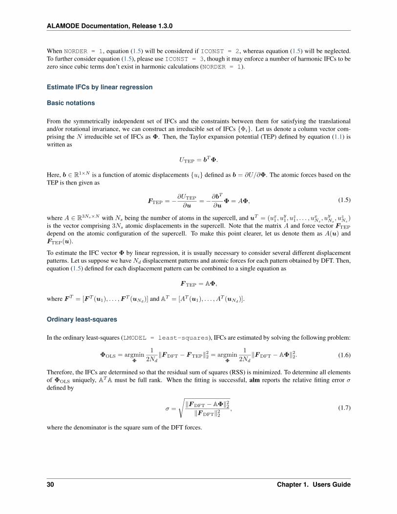
When NORDER = 1, equation (1.5) will be considered if ICONST = 2, whereas equation (1.5) will be neglected.To further consider equation (1.5), please use ICONST = 3, though it may enforce a number of harmonic IFCs to bezero since cubic terms don’t exist in harmonic calculations (NORDER = 1).
Estimate IFCs by linear regression
Basic notations
From the symmetrically independent set of IFCs and the constraints between them for satisfying the translationaland/or rotational invariance, we can construct an irreducible set of IFCs Φ𝑖. Let us denote a column vector com-prising the 𝑁 irreducible set of IFCs as Φ. Then, the Taylor expansion potential (TEP) defined by equation (1.1) iswritten as
𝑈TEP = 𝑏𝑇Φ.
Here, 𝑏 ∈ R1×𝑁 is a function of atomic displacements 𝑢𝑖 defined as 𝑏 = 𝜕𝑈/𝜕Φ. The atomic forces based on theTEP is then given as
𝐹TEP = −𝜕𝑈TEP
𝜕𝑢= −𝜕𝑏𝑇
𝜕𝑢Φ = 𝐴Φ, (1.5)
where 𝐴 ∈ R3𝑁𝑠×𝑁 with 𝑁𝑠 being the number of atoms in the supercell, and 𝑢𝑇 = (𝑢𝑥1 , 𝑢
𝑦1, 𝑢
𝑧1, . . . , 𝑢
𝑥𝑁𝑠
, 𝑢𝑦𝑁𝑠
, 𝑢𝑧𝑁𝑠
)is the vector comprising 3𝑁𝑠 atomic displacements in the supercell. Note that the matrix 𝐴 and force vector 𝐹TEP
depend on the atomic configuration of the supercell. To make this point clearer, let us denote them as 𝐴(𝑢) and𝐹TEP(𝑢).
To estimate the IFC vector Φ by linear regression, it is usually necessary to consider several different displacementpatterns. Let us suppose we have 𝑁𝑑 displacement patterns and atomic forces for each pattern obtained by DFT. Then,equation (1.5) defined for each displacement pattern can be combined to a single equation as
𝐹TEP = AΦ,
where 𝐹 𝑇 = [𝐹 𝑇 (𝑢1), . . . ,𝐹 𝑇 (𝑢𝑁𝑑)] and A𝑇 = [𝐴𝑇 (𝑢1), . . . , 𝐴𝑇 (𝑢𝑁𝑑
)].
Ordinary least-squares
In the ordinary least-squares (LMODEL = least-squares), IFCs are estimated by solving the following problem:
ΦOLS = argminΦ
1
2𝑁𝑑‖𝐹DFT − 𝐹TEP‖22 = argmin
Φ
1
2𝑁𝑑‖𝐹DFT − AΦ‖22. (1.6)
Therefore, the IFCs are determined so that the residual sum of squares (RSS) is minimized. To determine all elementsof ΦOLS uniquely, A𝑇A must be full rank. When the fitting is successful, alm reports the relative fitting error 𝜎defined by
𝜎 =
√‖𝐹DFT − AΦ‖22
‖𝐹DFT‖22, (1.7)
where the denominator is the square sum of the DFT forces.
30 Chapter 1. Users Guide
ALAMODE Documentation, Release 1.3.0
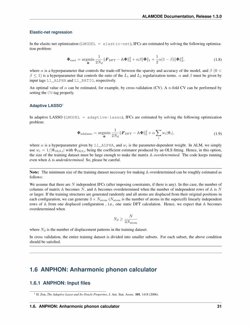
Elastic-net regression
In the elasitc-net optimization (LMODEL = elastic-net), IFCs are estimated by solving the following optimiza-tion problem:
Φenet = argminΦ
1
2𝑁𝑑‖𝐹DFT − AΦ‖22 + 𝛼𝛽‖Φ‖1 +
1
2𝛼(1 − 𝛽)‖Φ‖22, (1.8)
where 𝛼 is a hyperparameter that controls the trade-off between the sparsity and accuracy of the model, and 𝛽 (0 <𝛽 ≤ 1) is a hyperparameter that controls the ratio of the 𝐿1 and 𝐿2 regularization terms. 𝛼 and 𝛽 must be given byinput tags L1_ALPHA and L1_RATIO, respectively.
An optimal value of 𝛼 can be estimated, for example, by cross-validation (CV). A 𝑛-fold CV can be performed bysetting the CV-tag properly.
Adaptive LASSO1
In adaptive LASSO (LMODEL = adaptive-lasso), IFCs are estimated by solving the following optimizationproblem:
Φadalasso = argminΦ
1
2𝑁𝑑‖𝐹DFT − AΦ‖22 + 𝛼
∑𝑖
𝑤𝑖|Φ𝑖|, (1.9)
where 𝛼 is a hyperparameter given by L1_ALPHA, and 𝑤𝑖 is the parameter-dependent weight. In ALM, we simplyuse 𝑤𝑖 = 1/|ΦOLS,𝑖| with ΦOLS,𝑖 being the coefficient estimator produced by an OLS fitting. Hence, in this option,the size of the training dataset must be large enough to make the matrix A overdetermined. The code keeps runningeven when A is underdetermined. So, please be careful.
Note: The minimum size of the training dataset necessary for making A overdetermined can be roughly estimated asfollows:
We assume that there are 𝑁 independent IFCs (after imposing constraints, if there is any). In this case, the number ofcolumns of matrix A becomes 𝑁 , and A becomes overdetermined when the number of independent rows of A is 𝑁or larger. If the training structures are generated randomly and all atoms are displaced from their original positions ineach configuration, we can generate 3 ×𝑁atom (𝑁atom is the number of atoms in the supercell) linearly independentrows of A from one displaced configuration , i.e., one static DFT calculation. Hence, we expect that A becomesoverdetermined when
𝑁𝑑 ≥ 𝑁
3𝑁atom
where 𝑁𝑑 is the number of displacement patterns in the training dataset.
In cross validation, the entire training dataset is divided into smaller subsets. For each subset, the above conditionshould be satisfied.
1.6 ANPHON: Anharmonic phonon calculator
1.6.1 ANPHON: Input files
1 H. Zou, The Adaptive Lasso and Its Oracle Properties, J. Am. Stat. Assoc. 101, 1418 (2006).
1.6. ANPHON: Anharmonic phonon calculator 31
ALAMODE Documentation, Release 1.3.0
Format of input files
Each input file should consist of entry fields. Available entry fields are
&general, &cell, &analysis, and &kpoint.
The format of the input file is the same as that of alm which can be found here.
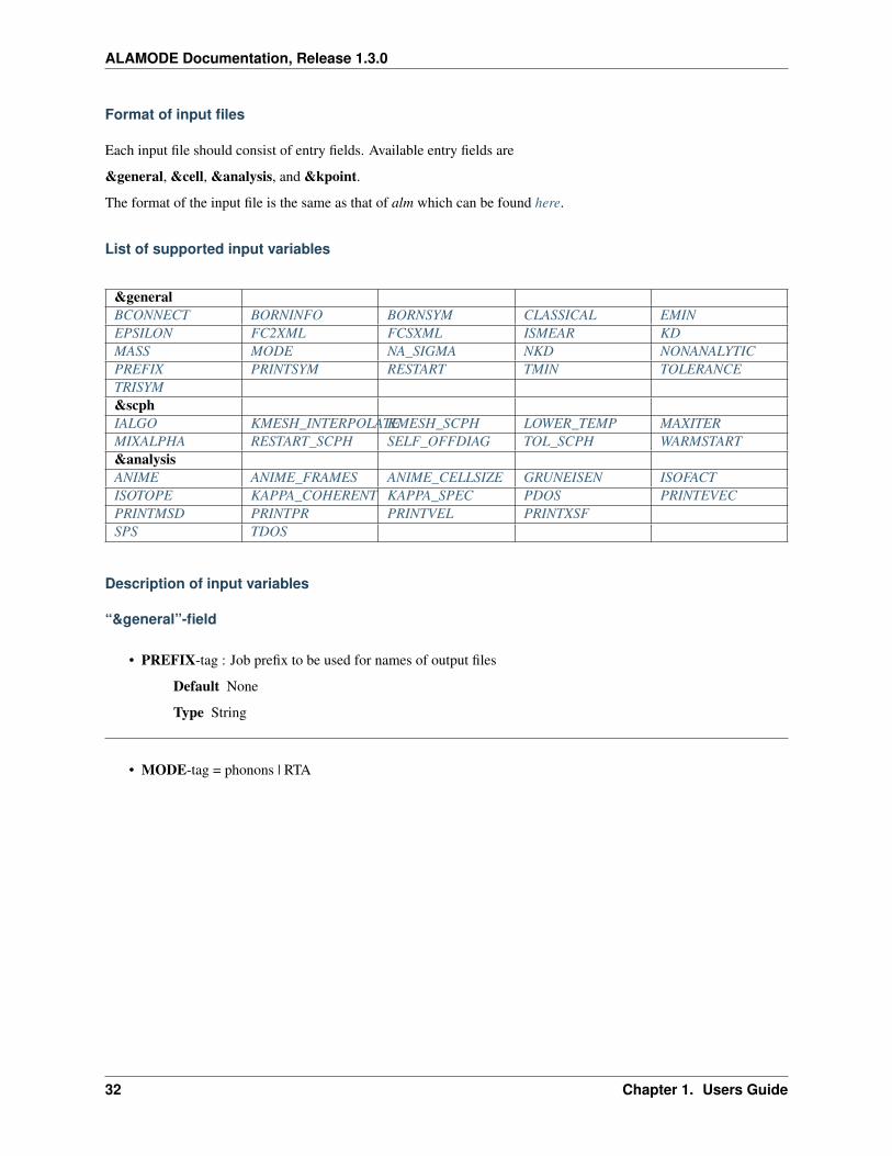
List of supported input variables
&generalBCONNECT BORNINFO BORNSYM CLASSICAL EMINEPSILON FC2XML FCSXML ISMEAR KDMASS MODE NA_SIGMA NKD NONANALYTICPREFIX PRINTSYM RESTART TMIN TOLERANCETRISYM&scphIALGO KMESH_INTERPOLATEKMESH_SCPH LOWER_TEMP MAXITERMIXALPHA RESTART_SCPH SELF_OFFDIAG TOL_SCPH WARMSTART&analysisANIME ANIME_FRAMES ANIME_CELLSIZE GRUNEISEN ISOFACTISOTOPE KAPPA_COHERENT KAPPA_SPEC PDOS PRINTEVECPRINTMSD PRINTPR PRINTVEL PRINTXSFSPS TDOS
Description of input variables
“&general”-field
• PREFIX-tag : Job prefix to be used for names of output files
Default None
Type String
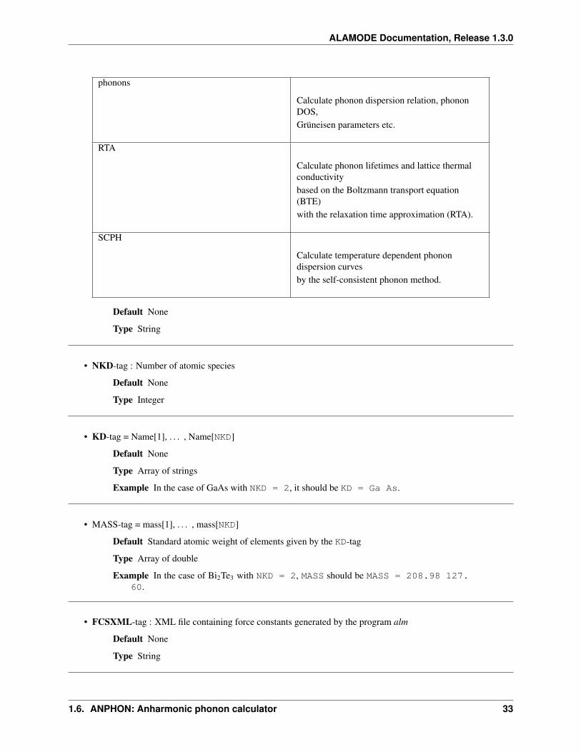
• MODE-tag = phonons | RTA
32 Chapter 1. Users Guide
ALAMODE Documentation, Release 1.3.0
phonons
Calculate phonon dispersion relation, phononDOS,Grüneisen parameters etc.
RTA
Calculate phonon lifetimes and lattice thermalconductivitybased on the Boltzmann transport equation(BTE)with the relaxation time approximation (RTA).
SCPH
Calculate temperature dependent phonondispersion curvesby the self-consistent phonon method.
Default None
Type String
• NKD-tag : Number of atomic species
Default None
Type Integer
• KD-tag = Name[1], . . . , Name[NKD]
Default None
Type Array of strings
Example In the case of GaAs with NKD = 2, it should be KD = Ga As.
• MASS-tag = mass[1], . . . , mass[NKD]
Default Standard atomic weight of elements given by the KD-tag
Type Array of double
Example In the case of Bi2Te3 with NKD = 2, MASS should be MASS = 208.98 127.60.
• FCSXML-tag : XML file containing force constants generated by the program alm
Default None
Type String
1.6. ANPHON: Anharmonic phonon calculator 33
ALAMODE Documentation, Release 1.3.0
• FC2XML-tag : XML file containing harmonic force constants for different size of supercell
Default None
Type String
Description When FC2XML is given, the harmonic force constants in this file are used for cal-culating dynamical matrices. It is possible to use different size of supercell for harmonicand anharmonic terms, which are specified by FC2XML and FCSXML respectively.
• TOLERANCE-tag : Tolerance for finding symmetry operations
Default 1.0e-6
Type Double
• PRINTSYM-tag = 0 | 1
0 Symmetry operations won’t be saved in “SYMM_INFO_PRIM”1 Symmetry operations will be saved in “SYMM_INFO_PRIM”
Default 0
type Integer
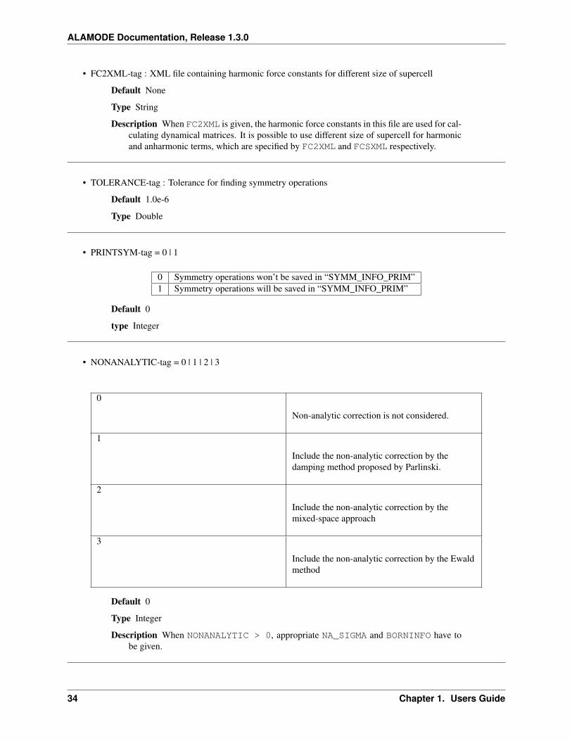
• NONANALYTIC-tag = 0 | 1 | 2 | 3
0
Non-analytic correction is not considered.
1
Include the non-analytic correction by thedamping method proposed by Parlinski.
2
Include the non-analytic correction by themixed-space approach
3
Include the non-analytic correction by the Ewaldmethod
Default 0
Type Integer
Description When NONANALYTIC > 0, appropriate NA_SIGMA and BORNINFO have tobe given.
34 Chapter 1. Users Guide
ALAMODE Documentation, Release 1.3.0
• NA_SIGMA-tag : Damping factor for the non-analytic term
Default 0.0
Type Double
Description Used when NONANALYTIC = 1. The definition of NA_SIGMA is described inthe formalism section.
• BORNINFO-tag : File containing the macroscopic dielectric tensor and Born effective charges for the non-analytic correction
Default None
Type String
Description The details of the file format can be found here.
• BORNSYM-tag = 0 | 1
0 Do not symmetrize Born effective charges1 Symmetrize Born effective charges by using point group symmetry
Default 0
Type Integer
• TMIN, TMAX, DT-tags : Temperature range and its stride in units of Kelvin
Default TMIN = 0, TMAX = 1000, DT = 10
Type Double
• EMIN, EMAX, DELTA_E-tags : Energy range and its stride in units of kayser (cm-1)
Default EMIN = 0, EMAX = 1000, DELTA_E = 10
Type Double
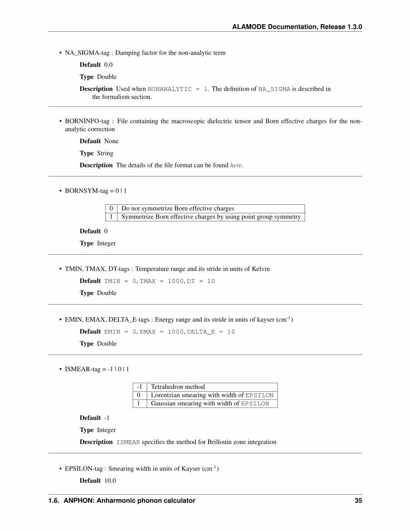
• ISMEAR-tag = -1 | 0 | 1
-1 Tetrahedron method0 Lorentzian smearing with width of EPSILON1 Gaussian smearing with width of EPSILON
Default -1
Type Integer
Description ISMEAR specifies the method for Brillouin zone integration
• EPSILON-tag : Smearing width in units of Kayser (cm-1)
Default 10.0
1.6. ANPHON: Anharmonic phonon calculator 35
ALAMODE Documentation, Release 1.3.0
Type Double
Description This variable is neglected when ISMEAR = -1
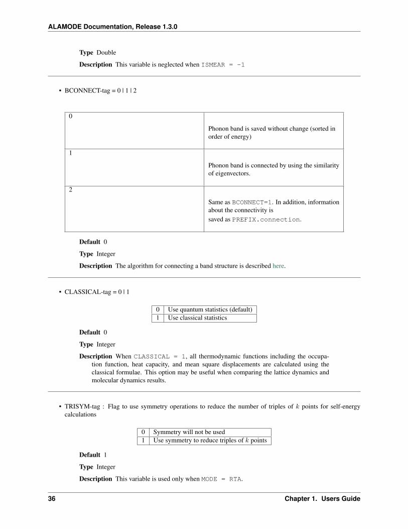
• BCONNECT-tag = 0 | 1 | 2
0
Phonon band is saved without change (sorted inorder of energy)
1
Phonon band is connected by using the similarityof eigenvectors.
2
Same as BCONNECT=1. In addition, informationabout the connectivity issaved as PREFIX.connection.
Default 0
Type Integer
Description The algorithm for connecting a band structure is described here.
• CLASSICAL-tag = 0 | 1
0 Use quantum statistics (default)1 Use classical statistics
Default 0
Type Integer
Description When CLASSICAL = 1, all thermodynamic functions including the occupa-tion function, heat capacity, and mean square displacements are calculated using theclassical formulae. This option may be useful when comparing the lattice dynamics andmolecular dynamics results.
• TRISYM-tag : Flag to use symmetry operations to reduce the number of triples of 𝑘 points for self-energycalculations
0 Symmetry will not be used1 Use symmetry to reduce triples of 𝑘 points
Default 1
Type Integer
Description This variable is used only when MODE = RTA.
36 Chapter 1. Users Guide
ALAMODE Documentation, Release 1.3.0
Note: TRISYM = 1 can reduce the computational cost, but phonon linewidth stored to the filePREFIX.result needs to be averaged at points of degeneracy. For that purpose, a subsidiary programanalyze_phonons.py* should be used.
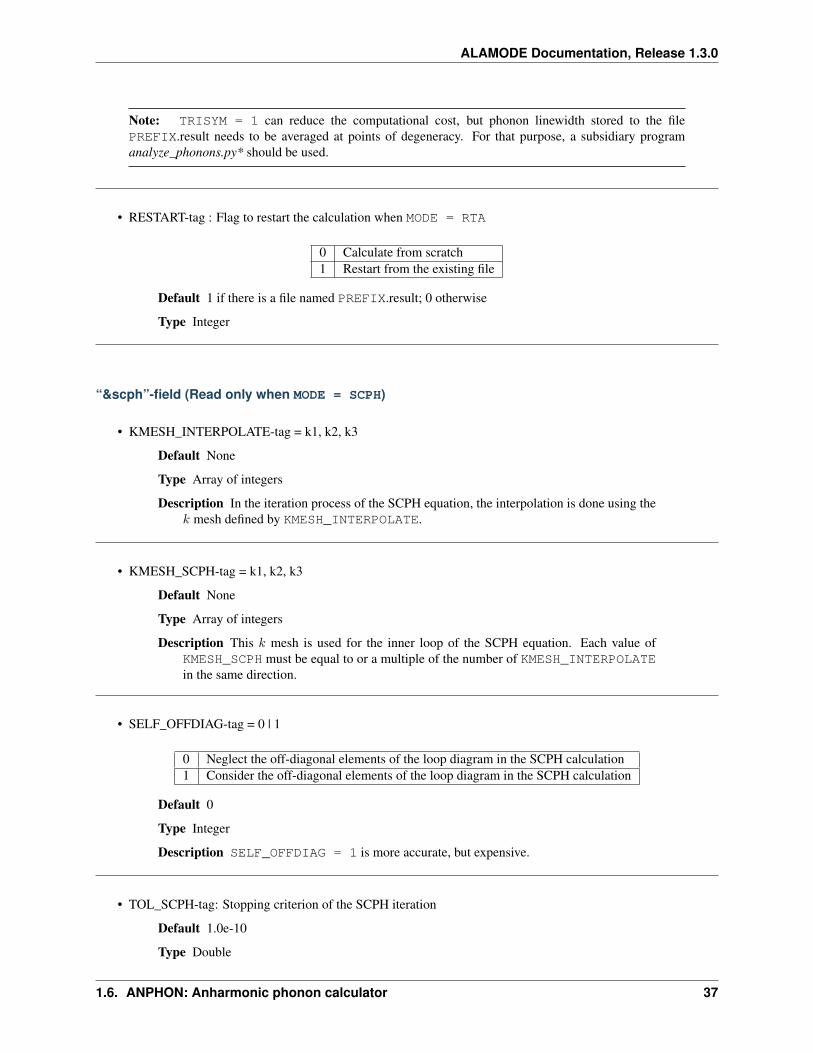
• RESTART-tag : Flag to restart the calculation when MODE = RTA
0 Calculate from scratch1 Restart from the existing file
Default 1 if there is a file named PREFIX.result; 0 otherwise
Type Integer
“&scph”-field (Read only when MODE = SCPH)
• KMESH_INTERPOLATE-tag = k1, k2, k3
Default None
Type Array of integers
Description In the iteration process of the SCPH equation, the interpolation is done using the𝑘 mesh defined by KMESH_INTERPOLATE.
• KMESH_SCPH-tag = k1, k2, k3
Default None
Type Array of integers
Description This 𝑘 mesh is used for the inner loop of the SCPH equation. Each value ofKMESH_SCPH must be equal to or a multiple of the number of KMESH_INTERPOLATEin the same direction.
• SELF_OFFDIAG-tag = 0 | 1
0 Neglect the off-diagonal elements of the loop diagram in the SCPH calculation1 Consider the off-diagonal elements of the loop diagram in the SCPH calculation
Default 0
Type Integer
Description SELF_OFFDIAG = 1 is more accurate, but expensive.
• TOL_SCPH-tag: Stopping criterion of the SCPH iteration
Default 1.0e-10
Type Double
1.6. ANPHON: Anharmonic phonon calculator 37

ALAMODE Documentation, Release 1.3.0
Description The SCPH iteration stops when both [ 1𝑁𝑞
∑𝑞(Ω
(𝑖)𝑞 −Ω
(𝑖−1)𝑞 )2]1/2 < TOL_SCPH
and (Ω(𝑖)𝑞 )2 ≥ 0 (∀𝑞) are satisfied. Here, Ω
(𝑖)𝑞 is the anharmonic phonon frequency
in the 𝑖th iteration and 𝑞 is the phonon modes at the irreducible momentum grid ofKMESH_INTERPOLATE.
• MIXALPHA-tag: Mixing parameter used in the SCPH iteration
Default 0.1
Type Double
• MAXITER-tag: Maximum number of the SCPH iteration
Default 1000
Type Integer
• LOWER_TEMP-tag = 0 | 1
0 The SCPH iteration start from TMIN to TMAX. (Raise the temperature)1 The SCPH iteration start from TMAX to TMIN. (Lower the temperature)
Default 1
Type Integer
• WARMSTART-tag = 0 | 1
0 SCPH iteration is initialized by harmonic frequencies and eigenvectors1 SCPH iteration is initialized by the solution of the previous temperature
Default 1
Type Integer
Description WARMSTART = 1 usually improves the convergence.
• IALGO-tag = 0 | 1
0 MPI parallelization for the 𝑘 point1 MPI parallelization for the phonon branch
Default 0
Type Integer
Description Use IALGO = 1 when the primitive cell contains many atoms and the numberof 𝑘 points is small.
• RESTART_SCPH-tag = 0 | 1
38 Chapter 1. Users Guide
ALAMODE Documentation, Release 1.3.0
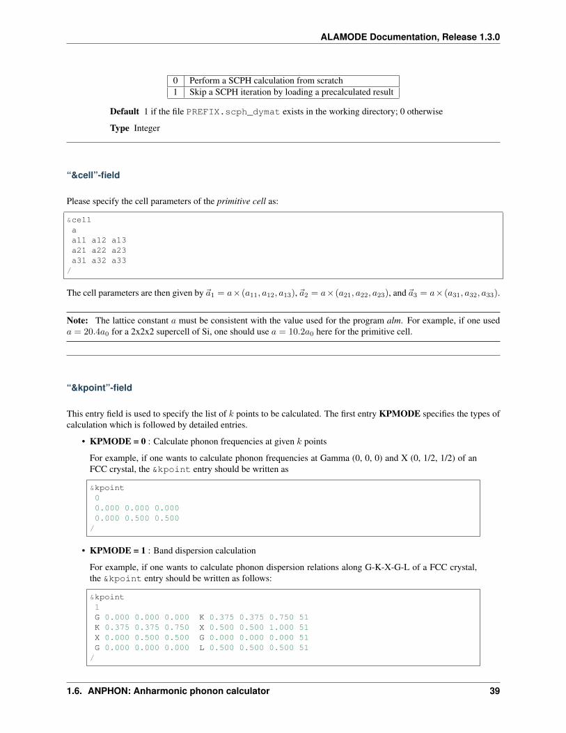
0 Perform a SCPH calculation from scratch1 Skip a SCPH iteration by loading a precalculated result
Default 1 if the file PREFIX.scph_dymat exists in the working directory; 0 otherwise
Type Integer
“&cell”-field
Please specify the cell parameters of the primitive cell as:
&cellaa11 a12 a13a21 a22 a23a31 a32 a33
/
The cell parameters are then given by 1 = 𝑎× (𝑎11, 𝑎12, 𝑎13), 2 = 𝑎× (𝑎21, 𝑎22, 𝑎23), and 3 = 𝑎× (𝑎31, 𝑎32, 𝑎33).
Note: The lattice constant 𝑎 must be consistent with the value used for the program alm. For example, if one used𝑎 = 20.4𝑎0 for a 2x2x2 supercell of Si, one should use 𝑎 = 10.2𝑎0 here for the primitive cell.
“&kpoint”-field
This entry field is used to specify the list of 𝑘 points to be calculated. The first entry KPMODE specifies the types ofcalculation which is followed by detailed entries.
• KPMODE = 0 : Calculate phonon frequencies at given 𝑘 points
For example, if one wants to calculate phonon frequencies at Gamma (0, 0, 0) and X (0, 1/2, 1/2) of anFCC crystal, the &kpoint entry should be written as
&kpoint00.000 0.000 0.0000.000 0.500 0.500/
• KPMODE = 1 : Band dispersion calculation
For example, if one wants to calculate phonon dispersion relations along G-K-X-G-L of a FCC crystal,the &kpoint entry should be written as follows:
&kpoint1G 0.000 0.000 0.000 K 0.375 0.375 0.750 51K 0.375 0.375 0.750 X 0.500 0.500 1.000 51X 0.000 0.500 0.500 G 0.000 0.000 0.000 51G 0.000 0.000 0.000 L 0.500 0.500 0.500 51/
1.6. ANPHON: Anharmonic phonon calculator 39
ALAMODE Documentation, Release 1.3.0
The 1st and 5th columns specify the character of Brillouin zone edges, which are followed by fractionalcoordinates of each point. The last column indicates the number of sampling points.
• KPMODE = 2 : Uniform 𝑘 grid for phonon DOS and thermal conductivity
In order to perform a calculation with 20x20x20 𝑘 grid, the entry should be
&kpoint220 20 20/
“&analysis”-field
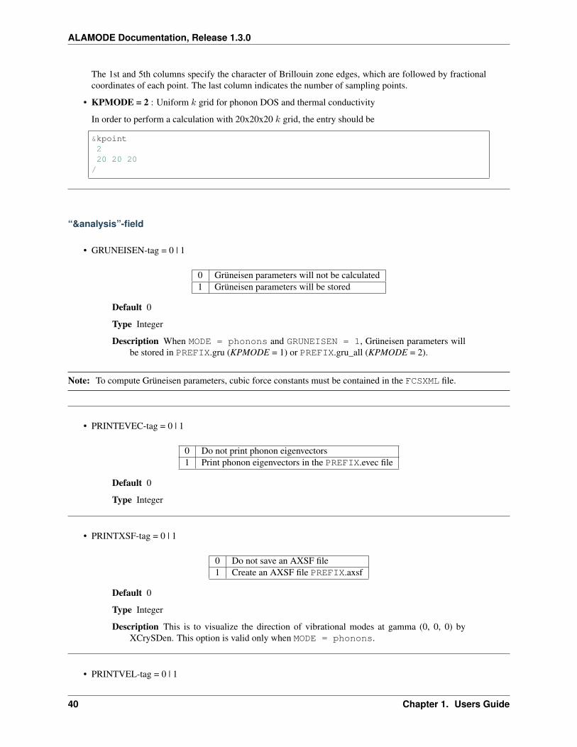
• GRUNEISEN-tag = 0 | 1
0 Grüneisen parameters will not be calculated1 Grüneisen parameters will be stored
Default 0
Type Integer
Description When MODE = phonons and GRUNEISEN = 1, Grüneisen parameters willbe stored in PREFIX.gru (KPMODE = 1) or PREFIX.gru_all (KPMODE = 2).
Note: To compute Grüneisen parameters, cubic force constants must be contained in the FCSXML file.
• PRINTEVEC-tag = 0 | 1
0 Do not print phonon eigenvectors1 Print phonon eigenvectors in the PREFIX.evec file
Default 0
Type Integer
• PRINTXSF-tag = 0 | 1
0 Do not save an AXSF file1 Create an AXSF file PREFIX.axsf
Default 0
Type Integer
Description This is to visualize the direction of vibrational modes at gamma (0, 0, 0) byXCrySDen. This option is valid only when MODE = phonons.
• PRINTVEL-tag = 0 | 1
40 Chapter 1. Users Guide
ALAMODE Documentation, Release 1.3.0
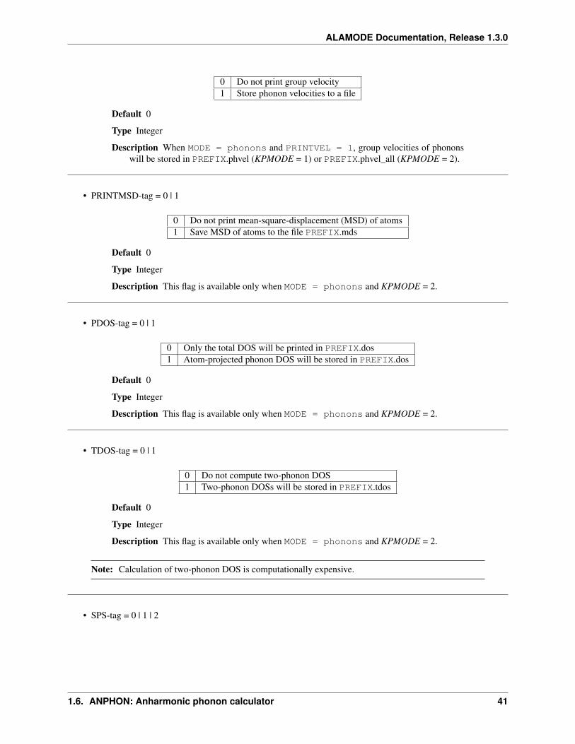
0 Do not print group velocity1 Store phonon velocities to a file
Default 0
Type Integer
Description When MODE = phonons and PRINTVEL = 1, group velocities of phononswill be stored in PREFIX.phvel (KPMODE = 1) or PREFIX.phvel_all (KPMODE = 2).
• PRINTMSD-tag = 0 | 1
0 Do not print mean-square-displacement (MSD) of atoms1 Save MSD of atoms to the file PREFIX.mds
Default 0
Type Integer
Description This flag is available only when MODE = phonons and KPMODE = 2.
• PDOS-tag = 0 | 1
0 Only the total DOS will be printed in PREFIX.dos1 Atom-projected phonon DOS will be stored in PREFIX.dos
Default 0
Type Integer
Description This flag is available only when MODE = phonons and KPMODE = 2.
• TDOS-tag = 0 | 1
0 Do not compute two-phonon DOS1 Two-phonon DOSs will be stored in PREFIX.tdos
Default 0
Type Integer
Description This flag is available only when MODE = phonons and KPMODE = 2.
Note: Calculation of two-phonon DOS is computationally expensive.
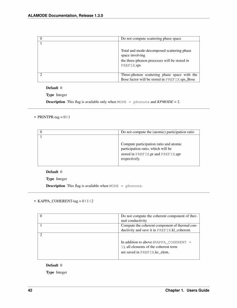
• SPS-tag = 0 | 1 | 2
1.6. ANPHON: Anharmonic phonon calculator 41
ALAMODE Documentation, Release 1.3.0
0 Do not compute scattering phase space1
Total and mode-decomposed scattering phasespace involvingthe three-phonon processes will be stored inPREFIX.sps
2 Three-phonon scattering phase space with theBose factor will be stored in PREFIX.sps_Bose
Default 0
Type Integer
Description This flag is available only when MODE = phonons and KPMODE = 2.
• PRINTPR-tag = 0 | 1
0 Do not compute the (atomic) participation ratio1
Compute participation ratio and atomicparticipation ratio, which will bestored in PREFIX.pr and PREFIX.aprrespectively.
Default 0
Type Integer
Description This flag is available when MODE = phonons.
• KAPPA_COHERENT-tag = 0 | 1 | 2
0 Do not compute the coherent component of ther-mal conductivity
1 Compute the coherent component of thermal con-ductivity and save it in PREFIX.kl_coherent.
2
In addition to above (KAPPA_COHERENT =1), all elements of the coherent termare saved in PREFIX.kc_elem.
Default 0
Type Integer
42 Chapter 1. Users Guide
ALAMODE Documentation, Release 1.3.0
Description This flag is available when MODE = RTA. For the theoretical details, please seethis page.
Caution: Still experimental. Please check the validity of results carefully.
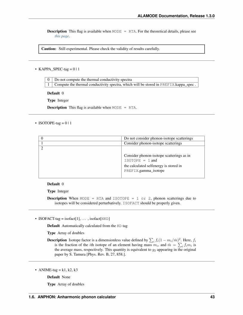
• KAPPA_SPEC-tag = 0 | 1
0 Do not compute the thermal conductivity spectra1 Compute the thermal conductivity spectra, which will be stored in PREFIX.kappa_spec .
Default 0
Type Integer
Description This flag is available when MODE = RTA.
• ISOTOPE-tag = 0 | 1
0 Do not consider phonon-isotope scatterings1 Consider phonon-isotope scatterings2
Consider phonon-isotope scatterings as inISOTOPE = 1 andthe calculated selfenergy is stored inPREFIX.gamma_isotope
Default 0
Type Integer
Description When MODE = RTA and ISOTOPE = 1 or 2, phonon scatterings due toisotopes will be considered perturbatively. ISOFACT should be properly given.
• ISOFACT-tag = isofact[1], . . . , isofact[NKD]
Default Automatically calculated from the KD tag
Type Array of doubles
Description Isotope factor is a dimensionless value defined by∑
𝑖 𝑓𝑖(1 −𝑚𝑖/)2. Here, 𝑓𝑖is the fraction of the 𝑖th isotope of an element having mass 𝑚𝑖, and =
∑𝑖 𝑓𝑖𝑚𝑖 is
the average mass, respectively. This quantity is equivalent to 𝑔2 appearing in the originalpaper by S. Tamura [Phys. Rev. B, 27, 858.].
• ANIME-tag = k1, k2, k3
Default None
Type Array of doubles
1.6. ANPHON: Anharmonic phonon calculator 43
ALAMODE Documentation, Release 1.3.0
Description This tag is to animate vibrational mode. k1, k2, and k3 specify the momentumof phonon modes to animate, which should be given in units of the reciprocal latticevector. For example, ANIME = 0.0 0.0 0.5 will animate phonon modes at (0, 0,1/2). When ANIME is given, ANIME_CELLSIZE is also necessary. You can choose theformat of animation files, either AXSF or XYZ, by ANIME_FORMAT tag.
• ANIME_FRAMES-tag: The number of frames saved in animation files
Default 20
Type Integer
• ANIME_CELLSIZE-tag = L1, L2, L3
Default None
Type Array of integers
Description This tag specifies the cell size for animation. L1, L2, and L3 should be largeenough to be commensurate with the reciprocal point given by the ANIME tag.
• ANIME_FORMAT = xsf | xyz
Default xyz
Type String
Description When ANIME_FORMAT = xsf, PREFIX.anime???.axsf files are created forXcrySDen. When ANIME_FORMAT = xyz, PREFIX.anime???.xyz files are createdfor VMD (and any other supporting software such as Jmol).
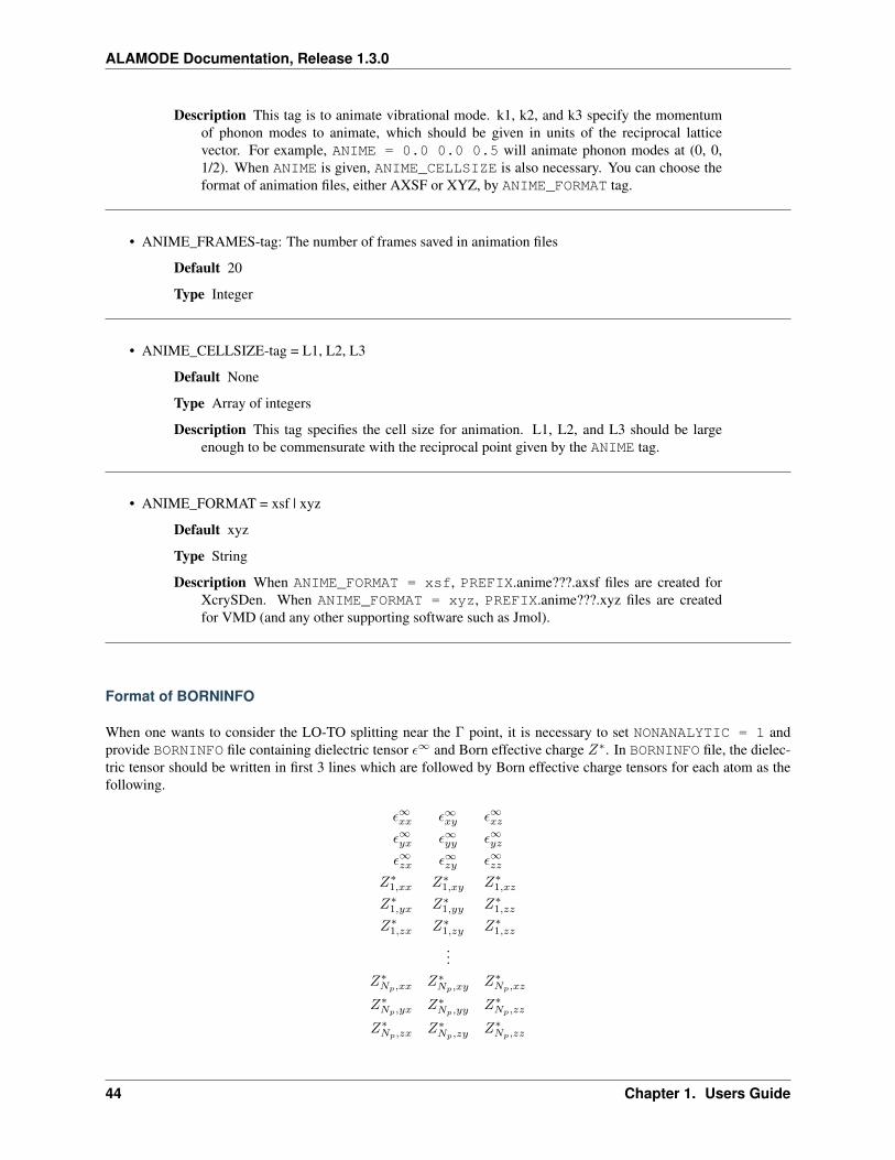
Format of BORNINFO
When one wants to consider the LO-TO splitting near the Γ point, it is necessary to set NONANALYTIC = 1 andprovide BORNINFO file containing dielectric tensor 𝜖∞ and Born effective charge 𝑍*. In BORNINFO file, the dielec-tric tensor should be written in first 3 lines which are followed by Born effective charge tensors for each atom as thefollowing.
𝜖∞𝑥𝑥 𝜖∞𝑥𝑦 𝜖∞𝑥𝑧
𝜖∞𝑦𝑥 𝜖∞𝑦𝑦 𝜖∞𝑦𝑧
𝜖∞𝑧𝑥 𝜖∞𝑧𝑦 𝜖∞𝑧𝑧
𝑍*1,𝑥𝑥 𝑍*
1,𝑥𝑦 𝑍*1,𝑥𝑧
𝑍*1,𝑦𝑥 𝑍*
1,𝑦𝑦 𝑍*1,𝑧𝑧
𝑍*1,𝑧𝑥 𝑍*
1,𝑧𝑦 𝑍*1,𝑧𝑧
...𝑍*𝑁𝑝,𝑥𝑥 𝑍*
𝑁𝑝,𝑥𝑦𝑍*𝑁𝑝,𝑥𝑧
𝑍*𝑁𝑝,𝑦𝑥 𝑍*
𝑁𝑝,𝑦𝑦𝑍*𝑁𝑝,𝑧𝑧
𝑍*𝑁𝑝,𝑧𝑥 𝑍*
𝑁𝑝,𝑧𝑦𝑍*𝑁𝑝,𝑧𝑧
44 Chapter 1. Users Guide
ALAMODE Documentation, Release 1.3.0
Here, 𝑁𝑝 is the number of atoms contained in the primitive cell.
Attention: Please pay attention to the order of Born effective charges.
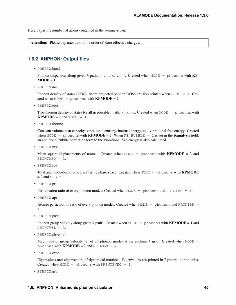
1.6.2 ANPHON: Output files
• PREFIX.bands
Phonon dispersion along given 𝑘 paths in units of cm -1. Created when MODE = phonons with KP-MODE = 1.
• PREFIX.dos
Phonon density of states (DOS). Atom projected phonon DOSs are also printed when PDOS = 1. Cre-ated when MODE = phonons with KPMODE = 2.
• PREFIX.tdos
Two-phonon density of states for all irreducible :math:’k’ points. Created when MODE = phononswithKPMODE = 2 and TDOS = 1.
• PREFIX.thermo
Constant volume heat capacity, vibrational entropy, internal energy, and vibrational free energy. Createdwhen MODE = phonons with KPMODE = 2. When FE_BUBBLE = 1 is set in the &analysis field,an additional bubble correction term to the vibrational free energy is also calculated.
• PREFIX.msd
Mean-square-displacements of atoms. Created when MODE = phonons with KPMODE = 2 andPRINTMSD = 1.
• PREFIX.sps
Total and mode-decomposed scattering phase space. Created when MODE = phonons with KPMODE= 2 and SPS = 1.
• PREFIX.pr
Participation ratio of every phonon modes. Created when MODE = phonons and PRINTPR = 1.
• PREFIX.apr
Atomic participation ratio of every phonon modes. Created when MODE = phonons and PRINTPR =1.
• PREFIX.phvel
Phonon group velocity along given 𝑘 paths. Created when MODE = phonons with KPMODE = 1 andPRINTVEL = 1.
• PREFIX.phvel_all
Magnitude of group velocity |𝑣| of all phonon modes at the uniform 𝑘 grid. Created when MODE =phonons with KPMODE = 2 and PRINTVEL = 1.
• PREFIX.evec
Eigenvalues and eigenvectors of dynamical matrices. Eigenvalues are printed in Rydberg atomic units.Created when MODE = phonons with PRINTEVEC = 1.
• PREFIX.gru
1.6. ANPHON: Anharmonic phonon calculator 45
ALAMODE Documentation, Release 1.3.0
Grüneisen parameters along given 𝑘 paths. Created when MODE = phonons with KPMODE = 1 andGRUNEISEN = 1.
• PREFIX.gru_all
Grüneisen parameters of all phonon modes at the uniform 𝑘 grid. Created when MODE = phononswith KPMODE = 2 and GRUNEISEN = 1.
• PREFIX.axsf
Zone-center phonon modes with directions indicated by arrows. This file can be visualized by XcrySDen.Created when MODE = phonons with PRINTXSF = 1.
• PREFIX.anime???.axsf and PREFIX.anime???.xyz
Files for animating phonon modes. ??? is the mode number. Created when MODE = phonons witha proper ANIME-tag. If ANIME_FORMAT = xsf, axsf files will be created which can be displayed byXcrySDen. If ANIME_FORMAT = xyz, xyz files will be created which can be visualized by VMD,Jmol, etc.
• PREFIX.result
In this file, phonon frequency, group velocity, and anharmonic phonon linewidths are printed. This file isupdated during thermal conductivity calculations (MODE = RTA). In addition, this file is read when therestart mode is turned on (RESTART = 1).
• PREFIX.kl
Lattice thermal conductivity tensor (Peierls term). Created when MODE = RTA.
• PREFIX.kl_spec
Spectra of lattice thermal conductivity. Only diagonal components are saved. Created when MODE =RTA and KAPPA_SPEC = 1.
• PREFIX.kl_coherent
Coherent component of lattice thermal conductivity. Created when KAPPA_COHERENT > 0 in MODE= RTA.
• PREFIX.kc_elem
Momentum- and mode-decomposed contributions to the coherent components of lattice thermal conduc-tivity. Created when KAPPA_COHERENT = 2 in MODE = RTA.
• PREFIX.gamma_isotope
Phonon selfenergy due to isotope scatterings calculated by the Tamura’s formula. Created when MODE =RTA and ISOTOPE = 2.
• PREFIX.scph_dymat
Anharmonic dynamical matrix calculated on the 𝑘 grid defined by the KMESH_INTERPOLATE tag. Thisfile is used to restart the SCPH calculation.
• PREFIX.scph_bands
Anharmonic phonon dispersion curves.
• PREFIX.scph_dos
Anharmonic phonon DOS. Created when MODE = SCPH and DOS = 1 with KPMODE = 2.
46 Chapter 1. Users Guide
ALAMODE Documentation, Release 1.3.0
• PREFIX.scph_thermo
Constant volume heat capacity, vibrational entropy, and vibrational free energy calculated based on theself-consistent phonon calculation. Created when MODE = SCPH with KPMODE = 2.
• PREFIX.scph_msd
Mean square displacement calculated within the SCPH theory. Created when MODE = SCPH andPRINTMSD = 1 with KPMODE = 2.
• PREFIX.scph_dfc2
This file contains ∆𝐷(𝑞) = 𝐷SCPH(𝑞) − 𝐷Harmonic(𝑞). For the definition, see the formalism of theSCPH calculation.
1.6.3 ANPHON: Theoretical background
Dynamical matrix
The dynamical matrix is given by
𝐷𝜇𝜈(𝜅𝜅′; 𝑞) =1√
𝑀𝜅𝑀𝜅′
∑ℓ′
Φ𝜇𝜈(ℓ𝜅; ℓ′𝜅′) exp [𝑖𝑞 · (𝑟(ℓ′) − 𝑟(ℓ))], (1.10)
where 𝑀𝜅 is the atomic mass of atom 𝜅. By diagonalizing the dynamical matrix, one can obtain 𝑚 (= 3𝑁𝜅) eigen-values 𝜔2
𝑞𝑗 (𝑗 = 1, 2, . . . ,𝑚) and corresponding eigenvectors 𝑒𝑞𝑗 for each 𝑞 point. Here, 𝑒𝑞𝑗 is a column vectorconsisting of atomic polarization 𝑒𝜇(𝜅; 𝑞𝑗). Let 𝐷(𝑞) denote a matrix form of equation (1.10), the eigenvalues maybe written as
𝜔2𝑞𝑗 = (𝑒*𝑞𝑗)
T𝐷(𝑞)𝑒𝑞𝑗 . (1.11)
Next, we introduce 𝑚 × 𝑚 matrices Λ and 𝑊 which are defined as Λ(𝑞) = diag(𝜔2𝑞1, . . . , 𝜔
2𝑞𝑚) and 𝑊 (𝑞) =
(𝑒𝑞1, . . . , 𝑒𝑞𝑚), respectively. Then, equation (1.11) can be denoted as
Λ(𝑞) = 𝑊 †(𝑞)𝐷(𝑞)𝑊 (𝑞).
When one needs to capture the LO-TO splitting near the zone-center by the supercell approach, it is necessary to addthe non-analytic part of the dynamical matrix defined by
𝐷NA𝜇𝜈 (𝜅𝜅′; 𝑞) =
1√𝑀𝜅𝑀𝜅′
4𝜋𝑒2
𝑉
(𝑍*𝜅𝑞)𝜇(𝑍*
𝜅′𝑞)𝜈𝑞 · 𝜖∞𝑞
,
where 𝑉 is the volume of the primitive cell, 𝑍*𝜅 is the Born effective charge tensor of atom 𝜅, and 𝜖∞ is the dielectric
constant tensor, respectively. In program anphon, either the Parlinski’s way1 or the mixed-space approach2 can beused. In the Parlinski’s approach (NONANALYTIC = 1), the total dynamical matrix is given by
𝐷(𝑞) + 𝐷NA(𝑞) exp (−𝑞2/𝜎2),
where 𝜎 is a damping factor. 𝜎 must be chosen carefully so that the non-analytic contribution becomes negligible atBrillouin zone boundaries. In the mixed-space approach (NONANALYTIC = 2), the total dynamical matrix is givenby
𝐷(𝑞) + 𝐷NA(𝑞)1
𝑁
∑ℓ′
exp [𝑖𝑞 · (𝑟(ℓ′) − 𝑟(ℓ))].
The second term vanishes at commensurate 𝑞 points other than Γ point (𝑞 = 0).
To include the non-analytic term, one needs to set NONANALYTIC > 0 and give appropriate BORNINFO andNA_SIGMA tags.
1 K. Parlinski, Z. Q. Li, and Y. Kawazoe, Phys. Rev. Lett. 81, 3298 (1998).2 Y. Wang et al., J. Phys.: Condens. Matter 22, 202201 (2010).
1.6. ANPHON: Anharmonic phonon calculator 47

ALAMODE Documentation, Release 1.3.0
Group velocity
The group velocity of phonon mode 𝑞𝑗 is given by
𝑣𝑞𝑗 =𝜕𝜔𝑞𝑗
𝜕𝑞.
To evaluate the group velocity numerically, we employ a central difference where 𝑣 may approximately be given by
𝑣𝑞𝑗 ≈𝜔𝑞+Δ𝑞𝑗 − 𝜔𝑞−Δ𝑞𝑗
2∆𝑞.
If one needs to save the group velocities, please turn on the PRINTVEL-tag.
Thermodynamics functions
The specific heat at constant volume 𝐶v, the internal energy 𝑈 , the vibrational entropy 𝑆, and the Helmholtz freeenergy 𝐹 of individual harmonic oscillator are given as follows:
𝑈 =1
𝑁𝑞
∑𝑞,𝑗
~𝜔𝑞𝑗
[1
𝑒~𝜔𝑞𝑗/𝑘𝑇 − 1+
1
2
],
𝐶v =𝑘
𝑁𝑞
∑𝑞,𝑗
(~𝜔𝑞𝑗
2𝑘𝑇
)2
cosech2
(~𝜔𝑞𝑗
2𝑘𝑇
),
𝑆 =𝑘
𝑁𝑞
∑𝑞,𝑗
[~𝜔𝑞𝑗
𝑘𝑇
1
𝑒~𝜔𝑞𝑗/𝑘𝑇 − 1− log
(1 − 𝑒−~𝜔𝑞𝑗/𝑘𝑇
)],
𝐹 =1
𝑁𝑞
∑𝑞,𝑗
[~𝜔𝑞𝑗
2+ 𝑘𝑇 log
(1 − 𝑒−~𝜔𝑞𝑗/𝑘𝑇
)].
Here, 𝑘 is the Boltzmann constant. These quantities are saved in the PREFIX.thermo file.
When the self-consistent phonon mode (MODE = SCPH) is selected, the anharmonic free-energy defined by the fol-lowing equation will be calculated and saved in the PREFIX.scph_thermo file:
𝐹 SCP =1
𝑁𝑞
∑𝑞,𝑗
[~Ω𝑞𝑗
2+ 𝑘𝑇 log
(1 − 𝑒−~Ω𝑞𝑗/𝑘𝑇
)]− 1
4𝑁𝑞
∑𝑞,𝑗
[Ω2
𝑞𝑗 − (𝐶†𝑞Λ(HA)
𝑞 𝐶𝑞)𝑗𝑗
]× ~[1 + 2𝑛𝑞𝑗 ]
2Ω𝑞𝑗.
Details of the derivation of the above expression can be found in Ref.7.
Mean square displacement
The mean square displacement tensor of atom 𝜅 is given by
⟨𝑢𝜇(𝜅)𝑢𝜈(𝜅)⟩ =~
2𝑀𝜅𝑁𝑞
∑𝑞,𝑗
1
2𝜔𝑞𝑗
(𝑒𝜇(𝜅; 𝑞𝑗)𝑒*𝜈(𝜅; 𝑞𝑗) + 𝑒*𝜇(𝜅; 𝑞𝑗)𝑒𝜈(𝜅; 𝑞𝑗)
)× coth
(~𝜔𝑞𝑗
2𝑘𝑇
). (1.12)
7 Y. Oba, T. Tadano, R. Akashi, and S. Tsuneyuki, Phys. Rev. Materials 3, 033601 (2019).
48 Chapter 1. Users Guide
ALAMODE Documentation, Release 1.3.0
When PRINTMSD is turned on, the code print the diagonal part of the mean square displacement tensor
⟨𝑢2𝜇(𝜅)
⟩=
~𝑀𝜅𝑁𝑞
∑𝑞,𝑗
1
𝜔𝑞𝑗|𝑒𝜇(𝜅; 𝑞𝑗)|2
(𝑛𝑞𝑗 +
1
2
),
where 𝑛𝑞𝑗 = 1/(𝑒~𝜔𝑞𝑗/𝑘𝑇 − 1) is the Bose-Einstein distribution function.
Phonon DOS
When KPMODE = 2, the program anphon saves the (one) phonon density of states (DOS) to the file PREFIX.dos.The one-phonon DOS is given by
DOS(𝜔) =1
𝑁𝑞
∑𝑞,𝑗
𝛿(𝜔 − 𝜔𝑞𝑗).
If PDOS = 1 is given, the program also prints the atom-projected phonon DOS which is given by
PDOS(𝜅;𝜔) =1
𝑁𝑞
∑𝑞,𝑗
|𝑒(𝜅; 𝑞𝑗)|2𝛿(𝜔 − 𝜔𝑞𝑗).
In addition, TDOS-tag is available to compute the two-phonon DOS defined by
DOS2(𝜔; 𝑞;±) =1
𝑁𝑞
∑𝑞1,𝑞2,𝑗1,𝑗2
𝛿(𝜔 ± 𝜔𝑞1𝑗1 − 𝜔𝑞2𝑗2)𝛿𝑞±𝑞1,𝑞2+𝐺,
where 𝐺 is a reciprocal lattice vector. The sign ± correspond to absorption and emission processes, respectively.Please note that the computation of the two-phonon DOS can be expensive especially when 𝑁𝑞 or 𝑁𝜅 is large.
(Atomic) participation ratio
Participation ratio (PR) and atomic participation ratio (APR) defined in the following may be useful to analyze thelocalized nature of the phonon mode 𝑞𝑗.
• Participation ratio (PR)
𝑃𝑅𝑞𝑗 =
(𝑁𝜅∑𝜅
|𝑒(𝜅; 𝑞𝑗)|2
𝑀𝜅
)2⧸𝑁𝜅
𝑁𝜅∑𝜅
|𝑒(𝜅; 𝑞𝑗)|4
𝑀2𝜅
• Atomic participation ratio (APR)
𝐴𝑃𝑅𝑞𝑗,𝜅 =|𝑒(𝜅; 𝑞𝑗)|2
𝑀𝜅
⧸(𝑁𝜅
𝑁𝜅∑𝜅
|𝑒(𝜅; 𝑞𝑗)|4
𝑀2𝜅
)1/2
For an extended eigenmode, the PR value is of order 1, whereas for a localized eigenmodes PR is of order 1/𝑁𝜅3.
APR is an atomic decomposition of PR that satisfies 𝑃𝑅𝑞𝑗 =∑
𝜅(𝐴𝑃𝑅𝑞𝑗,𝜅)2. To print the PR and APR, please setMODE = phonons and PRINTPR = 1 in the &analysis entry field.
3 J. Hafner and M. Krajci, J. Phys.: Condens. Matter 5, 2489 (1993).
1.6. ANPHON: Anharmonic phonon calculator 49
ALAMODE Documentation, Release 1.3.0
Scattering phase space
When KPMODE = 2 and SPS = 1, the three-phonon scattering phase space 𝑃3 is calculated and saved to the filePREFIX.sps. 𝑃3 is defined as
𝑃3(𝑞𝑗) =1
3𝑚3(2𝑃
(+)3 (𝑞𝑗) + 𝑃
(−)3 (𝑞𝑗)),
where 𝑚 is the number of phonon branches and
𝑃(±)3 (𝑞𝑗) =
1
𝑁𝑞
∑𝑞1,𝑞2,𝑗1,𝑗2
𝛿(𝜔𝑞𝑗 ± 𝜔𝑞1𝑗1 − 𝜔𝑞2𝑗2)𝛿𝑞±𝑞1,𝑞2+𝐺.
anphon also print the total scattering phase space
𝑃3 =1
𝑁𝑞
∑𝑞𝑗
𝑃3(𝑞𝑗).
When SPS = 2, the three-phonon scattering phase space with the occupation factor 𝑊 (±)3 will be calculated and
saved to the file PREFIX.sps_Bose. 𝑊 (±)3 is defined as
𝑊(±)3 (𝑞𝑗) =
1
𝑁𝑞
∑𝑞1,𝑞2,𝑗1,𝑗2
𝑛2 − 𝑛1
𝑛1 + 𝑛2 + 1
𝛿(𝜔𝑞𝑗 ± 𝜔𝑞1𝑗1 − 𝜔𝑞2𝑗2)𝛿𝑞±𝑞1,𝑞2+𝐺.
Here, 𝑛1 = 𝑛(𝜔𝑞1𝑗1) and 𝑛2 = 𝑛(𝜔𝑞2𝑗2) where 𝑛(𝜔) = 1𝑒~𝜔/𝑘𝐵𝑇−1
is the Bose-Einstein distribution function. Since
𝑛(𝜔) is temperature dependent, 𝑊 (±)3 is also temperature dependent. The file PREFIX.sps_Bose contains 𝑊 (±)
3 forall phonon modes at various temperatures specified with TMIN, TMAX, and DT tags.
Grüneisen parameter
The mode Grüneisen parameter, defined as 𝛾𝑞𝑗 = −𝜕 log𝜔𝑞𝑗
𝜕 log 𝑉 , is calculated by
𝛾𝑞𝑗 = −(𝑒*𝑞𝑗)
T𝛿𝐷(𝑞)𝑒𝑞𝑗
6𝜔2𝑞𝑗
,
where 𝛿𝐷(𝑞) is a change in the dynamical matrix due to a volume change 𝛿𝑉 , which is given by
𝛿𝐷𝜇𝜈(𝜅𝜅′; 𝑞) =1√
𝑀𝜅𝑀𝜅′
∑ℓ′
𝛿Φ𝜇𝜈(ℓ𝜅; ℓ′𝜅′) exp [𝑖𝑞 · (𝑟(ℓ′) − 𝑟(ℓ))], (1.13)
𝛿Φ𝜇𝜈(ℓ𝜅; ℓ′𝜅′) =∑
ℓ′′,𝜅′′,𝜆
Φ𝜇𝜈𝜆(ℓ𝜅; ℓ′𝜅′; ℓ′′𝜅′′)𝑟𝜆(ℓ′′𝜅′′). (1.14)
Please set GRUNEISEN = 1 and give an appropriate FCSXML file containing cubic IFCs to print Grüneisen parame-ters.
Anharmonic self-energy
The anharmonic self-energy due to cubic anharmonicity to the lowest order is given by
Σ𝑞𝑗(𝑖𝜔𝑚) =1
2~2∑𝑞1,𝑞2
∑𝑗1,𝑗2
|𝑉 (3)−𝑞𝑗,𝑞1𝑗1,𝑞2𝑗2
|2
×[
𝑛1 + 𝑛2 + 1
𝑖𝜔𝑚 + 𝜔1 + 𝜔2− 𝑛1 + 𝑛2 + 1
𝑖𝜔𝑚 − 𝜔1 − 𝜔2+
𝑛1 − 𝑛2
𝑖𝜔𝑚 − 𝜔1 + 𝜔2− 𝑛1 − 𝑛2
𝑖𝜔𝑚 + 𝜔1 − 𝜔2
],
50 Chapter 1. Users Guide

ALAMODE Documentation, Release 1.3.0
where 𝑖𝜔𝑚 is the Matsubara frequency. In equation (1.15), we simply denoted 𝜔𝑞𝑖𝑗𝑖 as 𝜔𝑖. The matrix element 𝑉 (3)
is given by
𝑉(3)𝑞𝑗,𝑞′𝑗′,𝑞′′𝑗′′ =
(~
2𝑁𝑞
) 32 1√𝜔𝑞𝑛𝜔𝑞′𝑗′𝜔𝑞′′𝑗′′
∑ℓ,ℓ′,ℓ′′
exp [i(𝑞 · 𝑟(ℓ) + 𝑞′ · 𝑟(ℓ′) + 𝑞′′ · 𝑟(ℓ′′))]
×∑
𝜅,𝜅′,𝜅′′
1√𝑀𝜅𝑀𝜅′𝑀𝜅′′
∑𝜇,𝜈,𝜆
Φ𝜇𝜈𝜆(ℓ𝜅; ℓ′𝜅′; ℓ′′𝜅′′)𝑒𝜇(𝜅; 𝑞𝑗)𝑒𝜈(𝜅′; 𝑞′𝑗′)𝑒𝜆(𝜅′′; 𝑞′′𝑗′′) ,
which becomes zero unless 𝑞 + 𝑞′ + 𝑞′′ is an integral multiple of 𝐺 = 𝑛1𝑏1 + 𝑛2𝑏2 + 𝑛3𝑏3. Phonon linewidth Γ𝑞𝑗 ,which is the imaginary part of the phonon self-energy, can be obtained by the analytic continuation to the real axis(𝑖𝜔𝑚 → 𝜔 + 𝑖0+) as
Γanh𝑞𝑗 (𝜔) =
𝜋
2~2∑𝑞1,𝑞2
∑𝑗1,𝑗2
|𝑉 (3)−𝑞𝑗,𝑞1𝑗1,𝑞2𝑗2
|2
× [−(𝑛1 + 𝑛2 + 1)𝛿(𝜔 + 𝜔1 + 𝜔2) + (𝑛1 + 𝑛2 + 1)𝛿(𝜔 − 𝜔1 − 𝜔2)
−(𝑛1 − 𝑛2)𝛿(𝜔 − 𝜔1 + 𝜔2) + (𝑛1 − 𝑛2)𝛿(𝜔 + 𝜔1 − 𝜔2)] .
The computation of equation (1.15) is the most expensive part of the thermal conductivity calculations. Therefore, weemploy the crystal symmetry to reduce the number of triplet pairs (𝑞𝑗, 𝑞′𝑗′, 𝑞′′𝑗′′) of 𝑉 (3) to calculate. To disable thereduction, please set TRISYM = 0.
Isotope scattering
The effect of isotope scatterings can be considered by the mass perturbation approach proposed by S. Tamura4 by theISOTOPE-tag. The corresponding phonon linewidth is given by
Γiso𝑞𝑗 (𝜔) =
𝜋
4𝑁𝑞𝜔2𝑞𝑗
∑𝑞1,𝑗1
𝛿(𝜔 − 𝜔𝑞1𝑗1)∑𝜅
𝑔2(𝜅)|𝑒*(𝜅; 𝑞1𝑗1) · 𝑒(𝜅; 𝑞𝑗)|2,
where 𝑔2 is a dimensionless factor given by
𝑔2(𝜅) =∑𝑖
𝑓𝑖(𝜅)
(1 − 𝑚𝑖(𝜅)
𝑀𝜅
)2
.
Here, 𝑓𝑖 is the fraction of the 𝑖th isotope of an element having mass 𝑚𝑖, and 𝑀𝜅 =∑
𝑖 𝑓𝑖𝑚𝑖(𝜅) is the average mass,respectively. The 𝑔2 values should be provided by the ISOFACT-tag. The average mass 𝑀𝜅 is substituted by the valuespecified in the MASS-tag.
Lattice thermal conductivity (Peierls term)
The lattice thermal conductivity tensor 𝜅𝜇𝜈ph(𝑇 ) is estimated within the relaxation-time approximation as
𝜅𝜇𝜈ph(𝑇 ) =
1
𝑉 𝑁𝑞
∑𝑞,𝑗
𝑐𝑞𝑗(𝑇 )𝑣𝜇𝑞𝑗𝑣𝜈𝑞𝑗𝜏𝑞𝑗(𝑇 ),
where 𝑉 is the unit cell volume, 𝑐𝑞𝑗 = ~𝜔𝑞𝑗𝜕𝑛𝑞𝑗/𝜕𝑇 , and 𝜏𝑞𝑗(𝑇 ) is the phonon lifetime. The phonon lifetime isestimated using the Matthiessen’s rule as
𝜏−1𝑞𝑗 (𝑇 ) = 2(Γanh
𝑞𝑗 (𝑇 ) + Γiso𝑞𝑗 ).
The lattice thermal conductivity is saved in the file PREFIX.kl.4 S. -I. Tamura, Phys. Rev. B 27, 858 (1983).
1.6. ANPHON: Anharmonic phonon calculator 51

ALAMODE Documentation, Release 1.3.0
The spectra of the lattice thermal conductivity 𝜅𝜇𝜇ph (𝜔) can also be calculated by setting KAPPA_SPEC = 1 in the
&analysis field. 𝜅𝜇𝜇ph (𝜔) is defined as
𝜅𝜇𝜇ph (𝜔) =
1
Ω𝑁𝑞
∑𝑞,𝑗
𝑐𝑞𝑗𝑣𝜇𝑞𝑗𝑣
𝜇𝑞𝑗𝜏𝑞𝑗𝛿(𝜔 − 𝜔𝑞𝑗).
If we integrate this quantity over 𝜔, we then obtain the bulk thermal conductivity, namely 𝜅𝜇𝜇ph =
∫∞0
𝜅𝜇𝜇ph (𝜔) d𝜔.
Cumulative thermal conductivity
The accumulative lattice thermal conductivity 𝜅𝜇𝜈ph,acc(𝐿) is defined as
𝜅𝜇𝜇ph,acc(𝐿) =
1
𝑉 𝑁𝑞
∑𝑞,𝑗
𝑐𝑞𝑗𝑣𝜇𝑞𝑗𝑣
𝜇𝑞𝑗𝜏𝑞𝑗Θ(𝐿− |𝑣𝑞𝑗 |𝜏𝑞𝑗),
where Θ(𝑥) is the step function. This quantity can be calculated by using the script analyze_phonons.py with--calc cumulative flag. One can also use another definition for the accumulative thermal conductivity:
𝜅𝜇𝜈ph,acc(𝐿) =
1
𝑉 𝑁𝑞
∑𝑞,𝑗
𝑐𝑞𝑗𝑣𝜇𝑞𝑗𝑣
𝜈𝑞𝑗𝜏𝑞𝑗Θ(𝐿− |𝑣𝜇𝑞𝑗 |𝜏𝑞𝑗).
In this case, the contribution to the total thermal conductivity is limited only from phonon modes whose mean-free-path along the 𝜇-direction is smaller than 𝐿. To calculate this, please use the --calc cumulative2 flag andspecify the direction 𝜇 by the --direction option.
Coherent component of lattice thermal conductivity
The coherent components of lattice thermal conductivity (see Ref.8), which are associated with the band off-diagonalcomponents of the harmonic heat-flux operator, is calculated as
𝜅𝜇𝜈c (𝑇 ) =
1
𝑉 𝑁𝑞
∑𝑞,𝑗𝑗′
𝑗 =𝑗′
𝑐𝑞𝑗𝜔𝑞𝑗′ + 𝑐𝑞𝑗′𝜔𝑞𝑗
𝜔𝑞𝑗 + 𝜔𝑞𝑗′𝑣𝜇𝑞𝑗𝑗′𝑣
𝜈𝑞𝑗′𝑗
Γ𝑞𝑗 + Γ𝑞𝑗′
(𝜔𝑞𝑗 − 𝜔𝑞𝑗′)2 + (Γ𝑞𝑗 + Γ𝑞𝑗′)2,
where 𝑐𝑞𝑗 = ~𝜔𝑞𝑗𝜕𝑛𝑞𝑗/𝜕𝑇 and Γ𝑞𝑗 is the total phonon linewidth (half width) of phonon mode 𝑞𝑗.
𝑣𝑞𝑗𝑗′ is a band off-diagonal generalization of the group velocity9. When KAPPA_COHERENT = 1 | 2 the coherentcomponent is calculated and saved in PREFIX.kl_coherent. When KAPPA_COHERENT = 2, all components of thecoherent term before summation are saved in PREFIX.kc_elem.
Delta function
To compute the phonon DOSs and the imaginary part of phonon self-energies, it is necessary to evaluate the Brillouin-zone integration containing Dirac’s delta function. For that purpose, we provide 3 options through the ISMEAR-tag.
When ISMEAR = 0, the delta function is replaced by the Lorentzian function as
𝛿(𝜔) ≈ 1
𝜋
𝜖2
𝜔2 + 𝜖2.
When ISMEAR = 1, the delta function is replaced by the Gaussian function as
𝛿(𝜔) ≈ 1√𝜋𝜖
exp (−𝜔2/𝜖2),
8 M. Simoncelli, N. Marzari, and F. Mauri, Nat. Phys. 15, 809 (2019).9 P. B. Allen and J. L. Feldman, Phys. Rev. B 48, 12581 (1993).
52 Chapter 1. Users Guide
ALAMODE Documentation, Release 1.3.0
which decays faster than the Lorentzian function. For both cases, 𝜖 should be given by the EPSILON-tag, which mustbe chosen carefully to avoid any unscientific results. 𝜖 should be small enough to capture detailed phonon structuressuch as phonon DOS or energy conservation surface related to three-phonon processes, but it should be large enoughto avoid unscientific oscillations. Choosing an appropriate value for 𝜖 is not a trivial task since it may depend on thephonon structure and the density of 𝑞 points.
To avoid such issues, the program anphon employs the tetrahedron method5 by default (ISMEAR = -1) for numericalevaluations of Brillouin zone integration containing 𝛿(𝜔). When the tetrahedron method is used, the EPSILON-tag isneglected. We recommend using the tetrahedron method whenever possible.
Self-consistent phonon (SCPH) calculation
The self-consistent phonon mode (MODE = SCPH) computes temperature-dependent phonon frequencies by solvingthe following equation self-consistently6:
𝑉[𝑛]𝑞𝑖𝑗 = 𝜔2
𝑞𝑖𝛿𝑖𝑗 +1
2
∑𝑞1,𝑘,ℓ
𝐹𝑞𝑞1,𝑖𝑗𝑘ℓ𝒦[𝑛−1]𝑞1,𝑘ℓ
. (1.15)
Here, 𝜔𝑞𝑗 is the harmonic phonon frequency and 𝐹𝑞𝑞1,𝑖𝑗𝑘ℓ = Φ(𝑞𝑖;−𝑞𝑗; 𝑞1𝑘;−𝑞1ℓ) is the reciprocal representationof fourth-order force constants. The updated phonon frequency in the 𝑛th iteration is obtained by diagonalizing thematrix 𝑉
[𝑛]𝑞𝑖𝑗 as
Λ[𝑛]𝑞 = 𝐶 [𝑛]†
𝑞 𝑉 [𝑛]𝑞 𝐶 [𝑛]
𝑞 ,
where 𝜔[𝑛]𝑞𝑗 = (Λ
[𝑛]𝑞𝑗𝑗)
12 and 𝐶
[𝑛]𝑞 is the unitary matrix that transforms the harmonic phonon eigenvectors into anhar-
monic ones as 𝑊 [𝑛]𝑞 = 𝑊𝑞𝐶
[𝑛]𝑞 . The matrix 𝒦 in Eq. (1.15) is defined as
𝒦[𝑛]𝑞,𝑖𝑗 = 𝛼𝐾
[𝑛]𝑞,𝑖𝑗 + (1 − 𝛼)𝐾
[𝑛−1]𝑞,𝑖𝑗 ,
𝐾[𝑛]𝑞,𝑖𝑗 =
∑𝑘
𝐶[𝑛]𝑞,𝑘𝑖𝐶
[𝑛]*𝑞,𝑘𝑗
~[1 + 2𝑛(𝜔
[𝑛]𝑞1𝑘
)]
2𝜔[𝑛]𝑞1𝑘
.
𝛼 is the mixing parameter, which can be changed via the MIXALPHA tag.
The SCPH equation is solved on the irreducible 𝑞 grid defined by the KMESH_INTERPOLATE tag. The 𝑞1 grid inEq. (1.15), given by the KMESH_SCPH tag, can be finer than the 𝑞 grid. After the SCPH iteration converges, the codecomputes the anharmonic correction to the harmonic force constant ∆𝐷(𝑟(ℓ)) as follows:
∆𝐷(𝑟(ℓ)) =1
𝑁𝑞
∑𝑞
∆𝐷(𝑞)𝑒−𝑖𝑞·𝑟(ℓ),
∆𝐷(𝑞) = 𝐷SCPH(𝑞) −𝐷Harmonic(𝑞),
𝐷SCPH(𝑞) = 𝑊𝑞𝐶[𝑛]𝑞 Λ[𝑛]
𝑞 𝐶 [𝑛]†𝑞 𝑊 †
𝑞 .
∆𝐷(𝑟(ℓ)) is saved in PREFIX.scph_dfc2.
The most computationally expensive part is the calculation of matrix elements of 𝐹𝑞𝑞1,𝑖𝑗𝑘ℓ. When SELF_OFFDIAG= 0 (default), the code only computes the elements of 𝐹𝑞𝑞1,𝑖𝑖𝑘𝑘. Therefore, the computational complexity is𝒪(𝑁 irred.
𝑞 𝑁𝑞1𝑚2). When SELF_OFFDIAG = 1, the off-diagonal elements are also calculated, and the computa-
tional complexity is 𝒪(𝑁 irred.𝑞 𝑁𝑞1𝑚
4).
5 P. E. Blöchl, O. Jepsen, and O. K. Andersen, Phys. Rev. B 49, 1450555 (1994).6 T. Tadano and S. Tsuneyuki, Phys. Rev. B 92, 054301 (2015).
1.6. ANPHON: Anharmonic phonon calculator 53
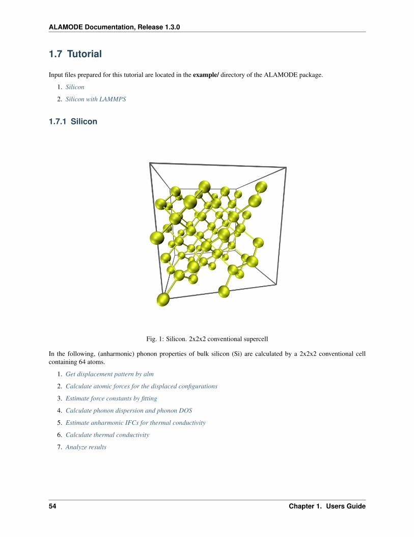
ALAMODE Documentation, Release 1.3.0
1.7 Tutorial
Input files prepared for this tutorial are located in the example/ directory of the ALAMODE package.
1. Silicon
2. Silicon with LAMMPS
1.7.1 Silicon
Fig. 1: Silicon. 2x2x2 conventional supercell
In the following, (anharmonic) phonon properties of bulk silicon (Si) are calculated by a 2x2x2 conventional cellcontaining 64 atoms.
1. Get displacement pattern by alm
2. Calculate atomic forces for the displaced configurations
3. Estimate force constants by fitting
4. Calculate phonon dispersion and phonon DOS
5. Estimate anharmonic IFCs for thermal conductivity
6. Calculate thermal conductivity
7. Analyze results
54 Chapter 1. Users Guide
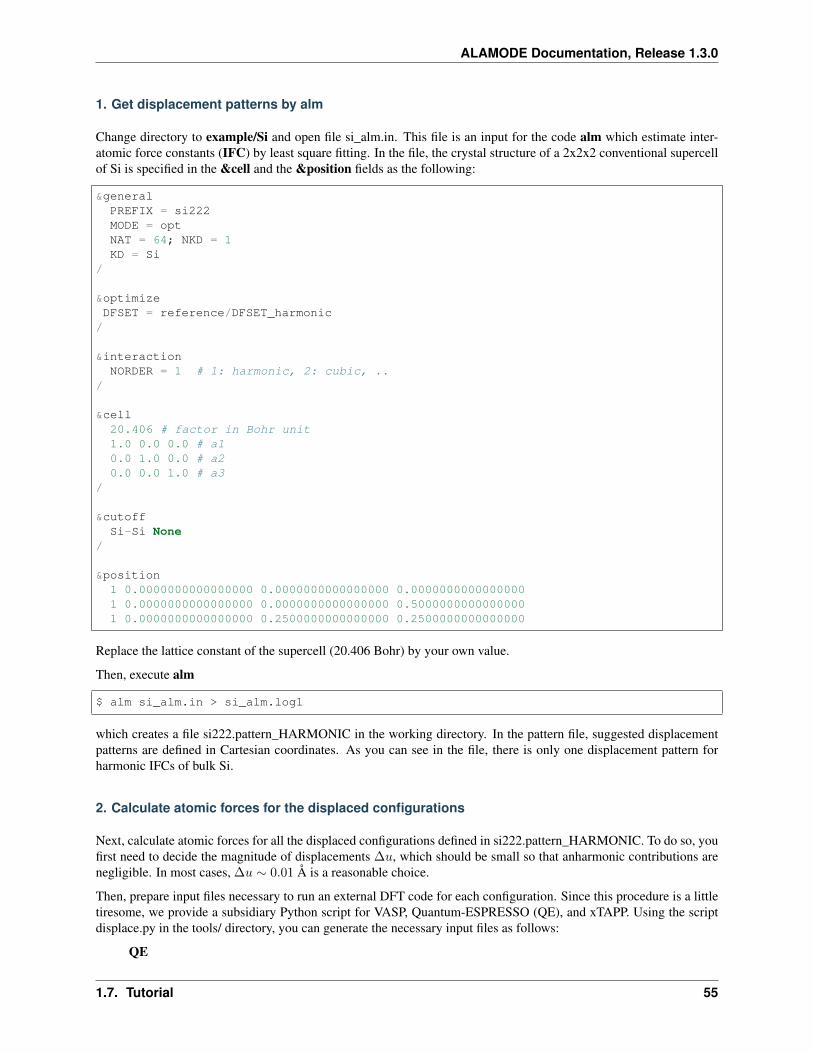
ALAMODE Documentation, Release 1.3.0
1. Get displacement patterns by alm
Change directory to example/Si and open file si_alm.in. This file is an input for the code alm which estimate inter-atomic force constants (IFC) by least square fitting. In the file, the crystal structure of a 2x2x2 conventional supercellof Si is specified in the &cell and the &position fields as the following:
&generalPREFIX = si222MODE = optNAT = 64; NKD = 1KD = Si
/
&optimizeDFSET = reference/DFSET_harmonic
/
&interactionNORDER = 1 # 1: harmonic, 2: cubic, ..
/
&cell20.406 # factor in Bohr unit1.0 0.0 0.0 # a10.0 1.0 0.0 # a20.0 0.0 1.0 # a3
/
&cutoffSi-Si None
/
&position1 0.0000000000000000 0.0000000000000000 0.00000000000000001 0.0000000000000000 0.0000000000000000 0.50000000000000001 0.0000000000000000 0.2500000000000000 0.2500000000000000
Replace the lattice constant of the supercell (20.406 Bohr) by your own value.
Then, execute alm
$ alm si_alm.in > si_alm.log1
which creates a file si222.pattern_HARMONIC in the working directory. In the pattern file, suggested displacementpatterns are defined in Cartesian coordinates. As you can see in the file, there is only one displacement pattern forharmonic IFCs of bulk Si.
2. Calculate atomic forces for the displaced configurations
Next, calculate atomic forces for all the displaced configurations defined in si222.pattern_HARMONIC. To do so, youfirst need to decide the magnitude of displacements ∆𝑢, which should be small so that anharmonic contributions arenegligible. In most cases, ∆𝑢 ∼ 0.01 Å is a reasonable choice.
Then, prepare input files necessary to run an external DFT code for each configuration. Since this procedure is a littletiresome, we provide a subsidiary Python script for VASP, Quantum-ESPRESSO (QE), and xTAPP. Using the scriptdisplace.py in the tools/ directory, you can generate the necessary input files as follows:
QE
1.7. Tutorial 55
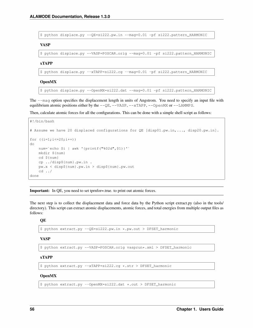
ALAMODE Documentation, Release 1.3.0
$ python displace.py --QE=si222.pw.in --mag=0.01 -pf si222.pattern_HARMONIC
VASP
$ python displace.py --VASP=POSCAR.orig --mag=0.01 -pf si222.pattern_HARMONIC
xTAPP
$ python displace.py --xTAPP=si222.cg --mag=0.01 -pf si222.pattern_HARMONIC
OpenMX
$ python displace.py --OpenMX=si222.dat --mag=0.01 -pf si222.pattern_HARMONIC
The --mag option specifies the displacement length in units of Angstrom. You need to specify an input file withequilibrium atomic positions either by the --QE, --VASP, --xTAPP, --OpenMX or --LAMMPS.
Then, calculate atomic forces for all the configurations. This can be done with a simple shell script as follows:
#!/bin/bash
# Assume we have 20 displaced configurations for QE [disp01.pw.in,..., disp20.pw.in].
for ((i=1;i<=20;i++))do
num=`echo $i | awk 'printf("%02d",$1)'`mkdir $numcd $numcp ../disp$num.pw.in .pw.x < disp$num.pw.in > disp$num.pw.outcd ../
done
Important: In QE, you need to set tprnfor=.true. to print out atomic forces.
The next step is to collect the displacement data and force data by the Python script extract.py (also in the tools/directory). This script can extract atomic displacements, atomic forces, and total energies from multiple output files asfollows:
QE
$ python extract.py --QE=si222.pw.in *.pw.out > DFSET_harmonic
VASP
$ python extract.py --VASP=POSCAR.orig vasprun*.xml > DFSET_harmonic
xTAPP
$ python extract.py --xTAPP=si222.cg *.str > DFSET_harmonic
OpenMX
$ python extract.py --OpenMX=si222.dat *.out > DFSET_harmonic
56 Chapter 1. Users Guide
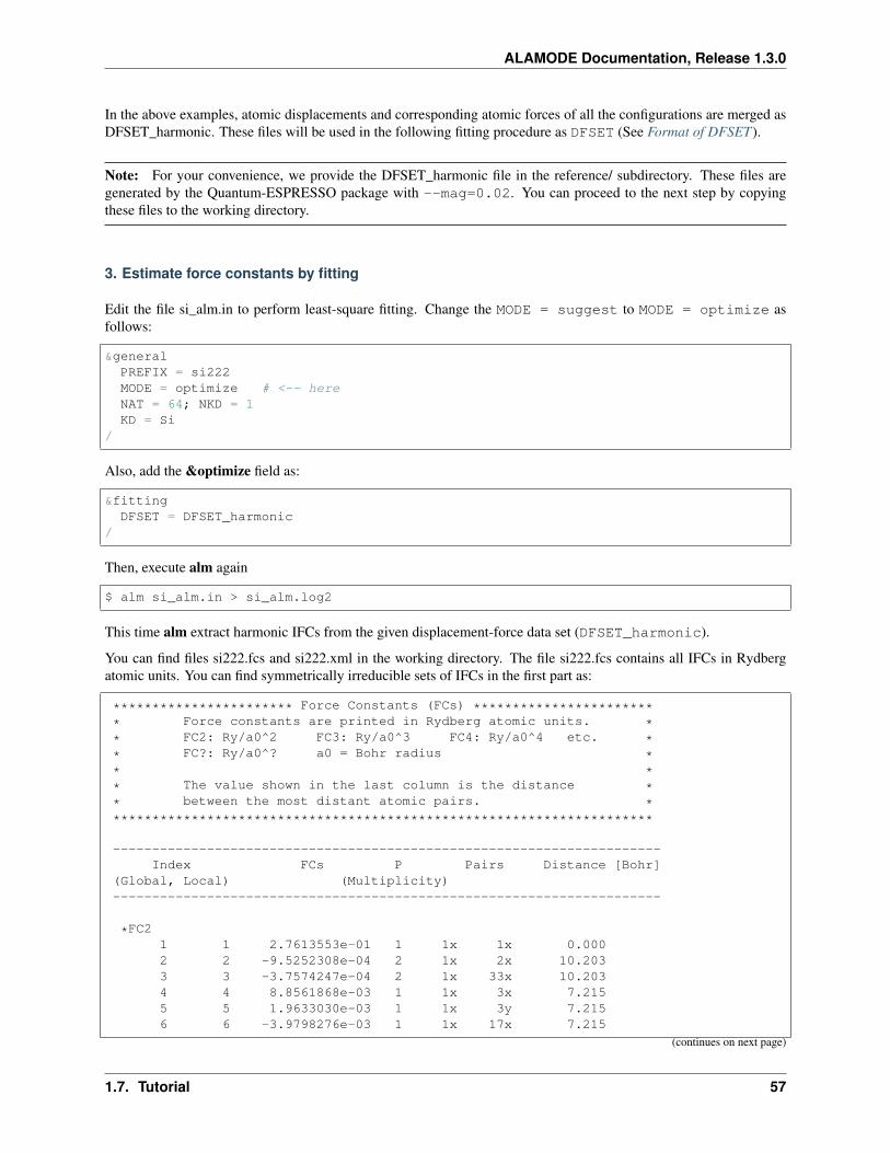
ALAMODE Documentation, Release 1.3.0
In the above examples, atomic displacements and corresponding atomic forces of all the configurations are merged asDFSET_harmonic. These files will be used in the following fitting procedure as DFSET (See Format of DFSET).
Note: For your convenience, we provide the DFSET_harmonic file in the reference/ subdirectory. These files aregenerated by the Quantum-ESPRESSO package with --mag=0.02. You can proceed to the next step by copyingthese files to the working directory.
3. Estimate force constants by fitting
Edit the file si_alm.in to perform least-square fitting. Change the MODE = suggest to MODE = optimize asfollows:
&generalPREFIX = si222MODE = optimize # <-- hereNAT = 64; NKD = 1KD = Si
/
Also, add the &optimize field as:
&fittingDFSET = DFSET_harmonic
/
Then, execute alm again
$ alm si_alm.in > si_alm.log2
This time alm extract harmonic IFCs from the given displacement-force data set (DFSET_harmonic).
You can find files si222.fcs and si222.xml in the working directory. The file si222.fcs contains all IFCs in Rydbergatomic units. You can find symmetrically irreducible sets of IFCs in the first part as:
*********************** Force Constants (FCs) ************************ Force constants are printed in Rydberg atomic units. ** FC2: Ry/a0^2 FC3: Ry/a0^3 FC4: Ry/a0^4 etc. ** FC?: Ry/a0^? a0 = Bohr radius ** ** The value shown in the last column is the distance ** between the most distant atomic pairs. **********************************************************************
----------------------------------------------------------------------Index FCs P Pairs Distance [Bohr]
(Global, Local) (Multiplicity)----------------------------------------------------------------------
*FC21 1 2.7613553e-01 1 1x 1x 0.0002 2 -9.5252308e-04 2 1x 2x 10.2033 3 -3.7574247e-04 2 1x 33x 10.2034 4 8.8561868e-03 1 1x 3x 7.2155 5 1.9633030e-03 1 1x 3y 7.2156 6 -3.9798276e-03 1 1x 17x 7.215
(continues on next page)
1.7. Tutorial 57
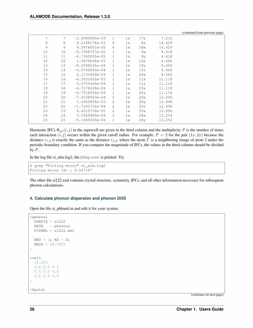
ALAMODE Documentation, Release 1.3.0
(continued from previous page)
7 7 -3.9080855e-03 1 1x 17z 7.2158 8 8.2188178e-03 4 1x 6x 14.4299 9 4.3878651e-05 4 1x 34x 14.429
10 10 -6.7358757e-02 1 1x 9x 4.41811 11 -4.7360832e-02 1 1x 9y 4.41812 12 1.0670028e-03 1 1x 10x 8.46013 13 -8.2098635e-04 1 1x 10y 8.46014 14 -6.9742830e-04 1 1x 10z 8.46015 15 2.1135669e-04 1 1x 26x 8.46016 16 -4.3031422e-03 1 1x 11x 11.11817 17 5.0759340e-04 1 1x 11y 11.11818 18 -4.7178438e-04 1 1x 25x 11.11819 19 -4.7518256e-04 1 1x 25z 11.11820 20 -7.4138963e-04 2 1x 20x 12.49621 21 1.2900836e-03 2 1x 20y 12.49622 22 -1.7263732e-04 2 1x 20z 12.49623 23 6.4515756e-05 2 1x 35x 12.49624 24 3.5369980e-04 1 1x 28x 13.25425 25 -5.1486930e-04 1 1x 28y 13.254
Harmonic IFCs Φ𝜇𝜈(𝑖, 𝑗) in the supercell are given in the third column and the multiplicity 𝑃 is the number of timeseach interaction (𝑖, 𝑗) occurs within the given cutoff radius. For example, 𝑃 = 2 for the pair (1𝑥, 2𝑥) because thedistance 𝑟1,2 is exactly the same as the distance 𝑟1,2′ where the atom 2’ is a neighboring image of atom 2 under theperiodic boundary condition. If you compare the magnitude of IFCs, the values in the third column should be dividedby 𝑃 .
In the log file si_alm.log2, the fitting error is printed. Try
$ grep "Fitting error" si_alm.log2Fitting error (%) : 0.567187
The other file si222.xml contains crystal structure, symmetry, IFCs, and all other information necessary for subsequentphonon calculations.
4. Calculate phonon dispersion and phonon DOS
Open the file si_phband.in and edit it for your system.
&generalPREFIX = si222MODE = phononsFCSXML = si222.xml
NKD = 1; KD = SiMASS = 28.0855
/
&cell10.2030.0 0.5 0.50.5 0.0 0.50.5 0.5 0.0
/
&kpoint
(continues on next page)
58 Chapter 1. Users Guide
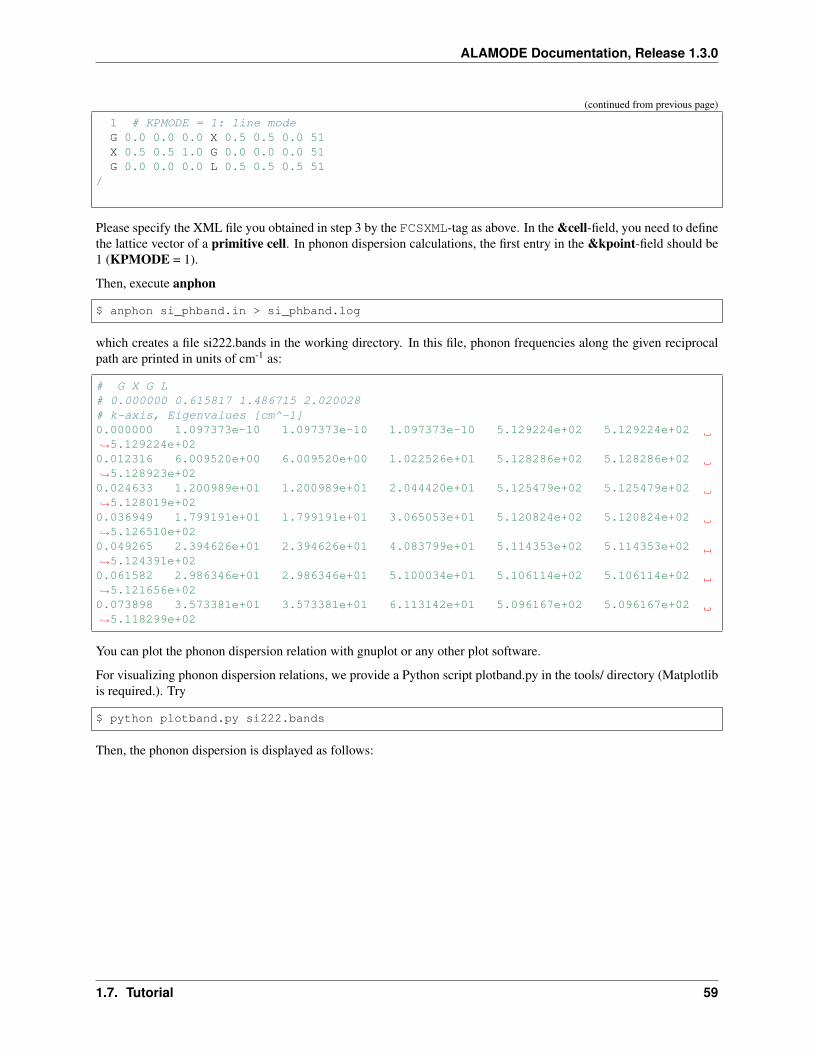
ALAMODE Documentation, Release 1.3.0
(continued from previous page)
1 # KPMODE = 1: line modeG 0.0 0.0 0.0 X 0.5 0.5 0.0 51X 0.5 0.5 1.0 G 0.0 0.0 0.0 51G 0.0 0.0 0.0 L 0.5 0.5 0.5 51
/
Please specify the XML file you obtained in step 3 by the FCSXML-tag as above. In the &cell-field, you need to definethe lattice vector of a primitive cell. In phonon dispersion calculations, the first entry in the &kpoint-field should be1 (KPMODE = 1).
Then, execute anphon
$ anphon si_phband.in > si_phband.log
which creates a file si222.bands in the working directory. In this file, phonon frequencies along the given reciprocalpath are printed in units of cm-1 as:
# G X G L# 0.000000 0.615817 1.486715 2.020028# k-axis, Eigenvalues [cm^-1]0.000000 1.097373e-10 1.097373e-10 1.097373e-10 5.129224e+02 5.129224e+02→˓5.129224e+020.012316 6.009520e+00 6.009520e+00 1.022526e+01 5.128286e+02 5.128286e+02→˓5.128923e+020.024633 1.200989e+01 1.200989e+01 2.044420e+01 5.125479e+02 5.125479e+02→˓5.128019e+020.036949 1.799191e+01 1.799191e+01 3.065053e+01 5.120824e+02 5.120824e+02→˓5.126510e+020.049265 2.394626e+01 2.394626e+01 4.083799e+01 5.114353e+02 5.114353e+02→˓5.124391e+020.061582 2.986346e+01 2.986346e+01 5.100034e+01 5.106114e+02 5.106114e+02→˓5.121656e+020.073898 3.573381e+01 3.573381e+01 6.113142e+01 5.096167e+02 5.096167e+02→˓5.118299e+02
You can plot the phonon dispersion relation with gnuplot or any other plot software.
For visualizing phonon dispersion relations, we provide a Python script plotband.py in the tools/ directory (Matplotlibis required.). Try
$ python plotband.py si222.bands
Then, the phonon dispersion is displayed as follows:
1.7. Tutorial 59
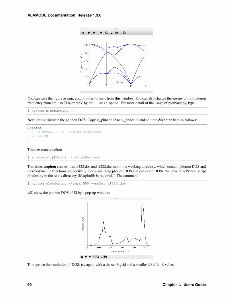
ALAMODE Documentation, Release 1.3.0
You can save the figure as png, eps, or other formats from this window. You can also change the energy unit of phononfrequency from cm-1 to THz or meV by the --unit option. For more detail of the usage of plotband.py, type
$ python plotband.py -h
Next, let us calculate the phonon DOS. Copy si_phband.in to si_phdos.in and edit the &kpoint field as follows:
&kpoint2 # KPMODE = 2: uniform mesh mode20 20 20
/
Then, execute anphon
$ anphon si_phdos.in > si_phdos.log
This time, anphon creates files si222.dos and si222.thermo in the working directory, which contain phonon DOS andthermodynamic functions, respectively. For visualizing phonon DOS and projected DOSs, we provide a Python scriptplotdos.py in the tools/ directory (Matplotlib is required.). The command
$ python plotdos.py --emax 550 --nokey si222.dos
will show the phonon DOS of Si by a pop-up window:
To improve the resolution of DOS, try again with a denser 𝑘 grid and a smaller DELTA_E value.
60 Chapter 1. Users Guide
ALAMODE Documentation, Release 1.3.0
5. Estimate cubic IFCs for thermal conductivity
Copy file si_alm.in to si_alm2.in. Edit the &general, &interaction, and &cutoff fields of si_alm2.in as the following:
&generalPREFIX = si222_cubicMODE = suggestNAT = 64; NKD = 1KD = Si
/
Change the PREFIX from si222 to si222_cubic and set MODE to suggest.
&interactionNORDER = 2
/
Change the NORDER tag from NORDER = 1 to NORDER = 2 to include cubic IFCs. Here, we consider cubicinteraction pairs up to second nearest neighbors by specifying the cutoff radii as:
&cutoffSi-Si None 7.3
/
7.3 Bohr is slightly larger than the distance of second nearest neighbors (7.21461 Bohr). Change the cutoff valueappropriately for your own case. (Atomic distance can be found in the file si_alm.log.)
Then, execute alm
$ alm si_alm2.in > si_alm2.log
which creates files si222_cubic.pattern_HARMONIC and si222_cubic.pattern_ANHARM3.
Then, calculate atomic forces of displaced configurations given in the file si222_cubic.pattern_ANHARM3, and collectthe displacement and force datasets to a file DFSET_cubic as you did for harmonic IFCs in Steps 3 and 4.
Note: Since making DFSET_cubic requires moderate computational resources, you can skip this procedure bycopying file reference/DFSET_cubic to the working directory. The file we provide is generated by the Quantum-ESPRESSO package with --mag=0.04.
In si_alm2.in, change MODE = suggest to MODE = optimize and add the following:
&optimizeDFSET = DFSET_cubicFC2XML = si222.xml # Fix harmonic IFCs
/
By the FC2XML tag, harmonic IFCs are fixed to the values in si222.xml. Then, execute alm again
$ alm si_alm2.in > si_alm2.log2
which creates files si222_cubic.fcs and si222_cubic.xml. This time cubic IFCs are also included in these files.
Note: In the above example, we obtained cubic IFCs by least square fitting with harmonic IFCs being fixed to thevalue of the previous harmonic calculation. You can also estimate both harmonic and cubic IFCs simultaneouslyinstead. To do this, merge DFSET_harmonic and DFSET_cubic as
1.7. Tutorial 61
ALAMODE Documentation, Release 1.3.0
$ cat DFSET_harmonic DFSET_cubic > DFSET_merged
and change the &fitting field as the following:
&fittingDFSET = DFSET_merged
/
6. Calculate thermal conductivity
Copy file si_phdos.in to si_RTA.in and edit the MODE and FCSXML tags as follows:
&generalPREFIX = si222MODE = RTAFCSXML = si222_cubic.xml
NKD = 1; KD = SiMASS = 28.0855
/
In addition, change the 𝑘 grid density as:
&kpoint210 10 10
/
Then, execute anphon as a background job
$ anphon si_RTA.in > si_RTA.log &
Please be patient. This can take a while. When the job finishes, you can find a file si222.kl in which the lattice thermalconductivity is saved. You can plot this file using gnuplot (or any other plotting softwares) as follows:
$ gnuplotgnuplot> set logscale xygnuplot> set xlabel "Temperature (K)"gnuplot> set ylabel "Lattice thermal conductivity (W/mK)"gnuplot> plot "si222.kl" usi 1:2 w lp
As you can see, the thermal conductivity diverges in 𝑇 → 0 limit. This occurs because we only considered intrinsicphonon-phonon scatterings in the present calculation and neglected phonon-boundary scatterings which are domi-nant in the low-temperature range. The effect of the boundary scattering can be included using the python scriptanalyze_phonons.py in the tools directory:
$ analyze_phonons.py --calc kappa_boundary --size 1.0e+6 si222.result > si222_→˓boundary_1mm.kl
In this script, the phonon lifetimes are altered using the Matthiessen’s rule
1
𝜏 𝑡𝑜𝑡𝑎𝑙𝑞
=1
𝜏𝑝−𝑝𝑞
+2|𝑣𝑞|𝐿
.
Here, the first term on the right-hand side of the equation is the scattering rate due to the phonon-phonon scatteringand the second term is the scattering rate due to a grain boundary of size 𝐿. The size 𝐿 must be specified using the
62 Chapter 1. Users Guide
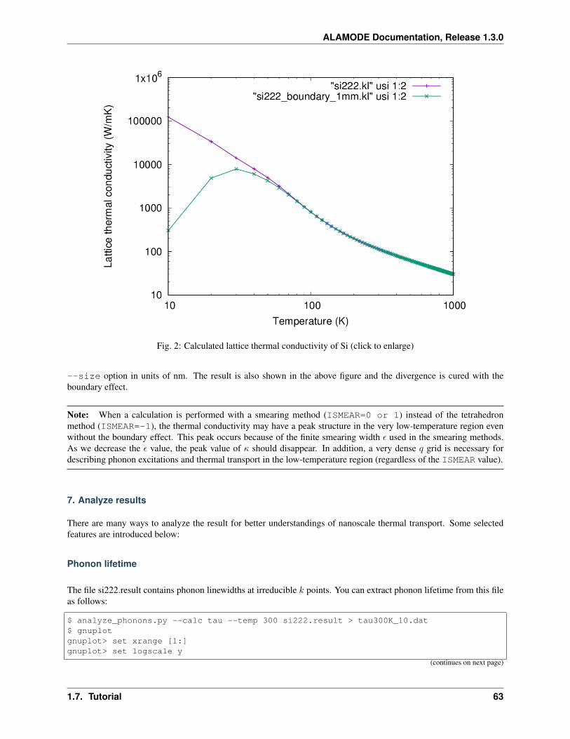
ALAMODE Documentation, Release 1.3.0
Fig. 2: Calculated lattice thermal conductivity of Si (click to enlarge)
--size option in units of nm. The result is also shown in the above figure and the divergence is cured with theboundary effect.
Note: When a calculation is performed with a smearing method (ISMEAR=0 or 1) instead of the tetrahedronmethod (ISMEAR=-1), the thermal conductivity may have a peak structure in the very low-temperature region evenwithout the boundary effect. This peak occurs because of the finite smearing width 𝜖 used in the smearing methods.As we decrease the 𝜖 value, the peak value of 𝜅 should disappear. In addition, a very dense 𝑞 grid is necessary fordescribing phonon excitations and thermal transport in the low-temperature region (regardless of the ISMEAR value).
7. Analyze results
There are many ways to analyze the result for better understandings of nanoscale thermal transport. Some selectedfeatures are introduced below:
Phonon lifetime
The file si222.result contains phonon linewidths at irreducible 𝑘 points. You can extract phonon lifetime from this fileas follows:
$ analyze_phonons.py --calc tau --temp 300 si222.result > tau300K_10.dat$ gnuplotgnuplot> set xrange [1:]gnuplot> set logscale y
(continues on next page)
1.7. Tutorial 63
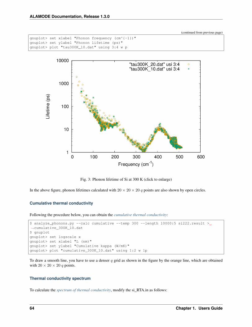
ALAMODE Documentation, Release 1.3.0
(continued from previous page)
gnuplot> set xlabel "Phonon frequency (cm^-1)"gnuplot> set ylabel "Phonon lifetime (ps)"gnuplot> plot "tau300K_10.dat" using 3:4 w p
Fig. 3: Phonon lifetime of Si at 300 K (click to enlarge)
In the above figure, phonon lifetimes calculated with 20 × 20 × 20 𝑞 points are also shown by open circles.
Cumulative thermal conductivity
Following the procedure below, you can obtain the cumulative thermal conductivity:
$ analyze_phonons.py --calc cumulative --temp 300 --length 10000:5 si222.result >→˓cumulative_300K_10.dat$ gnuplotgnuplot> set logscale xgnuplot> set xlabel "L (nm)"gnuplot> set ylabel "Cumulative kappa (W/mK)"gnuplot> plot "cumulative_300K_10.dat" using 1:2 w lp
To draw a smooth line, you have to use a denser 𝑞 grid as shown in the figure by the orange line, which are obtainedwith 20 × 20 × 20 𝑞 points.
Thermal conductivity spectrum
To calculate the spectrum of thermal conductivity, modify the si_RTA.in as follows:
64 Chapter 1. Users Guide
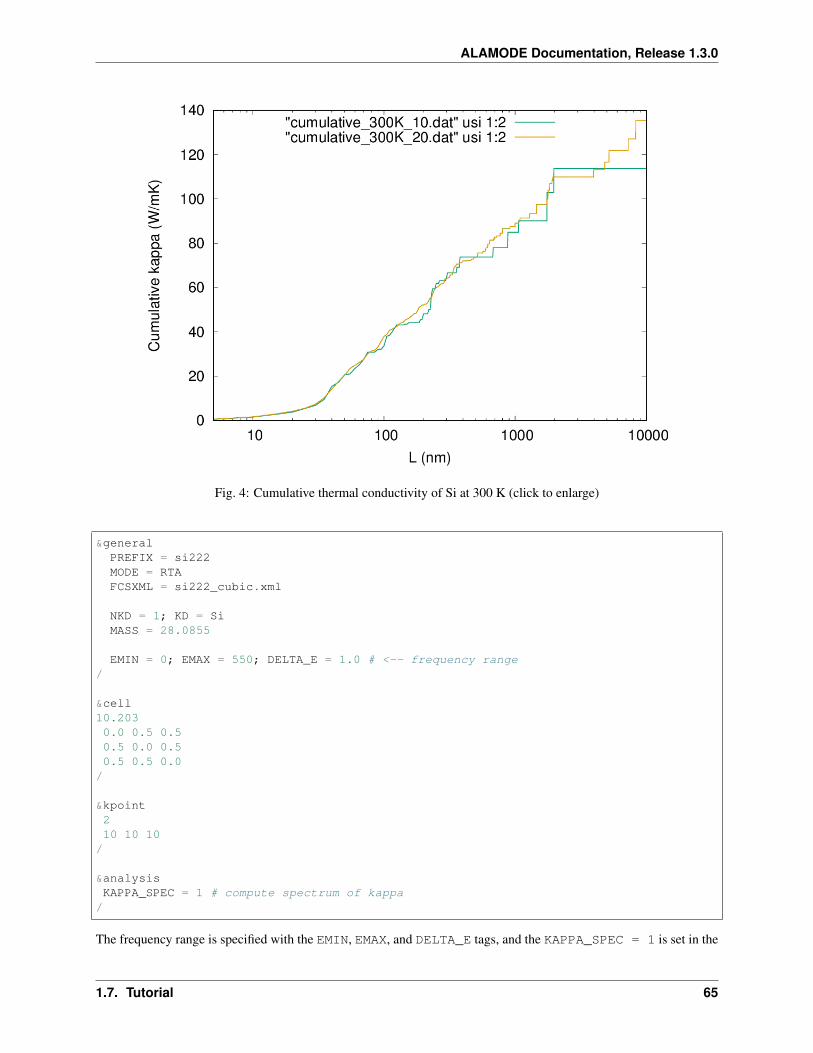
ALAMODE Documentation, Release 1.3.0
Fig. 4: Cumulative thermal conductivity of Si at 300 K (click to enlarge)
&generalPREFIX = si222MODE = RTAFCSXML = si222_cubic.xml
NKD = 1; KD = SiMASS = 28.0855
EMIN = 0; EMAX = 550; DELTA_E = 1.0 # <-- frequency range/
&cell10.2030.0 0.5 0.50.5 0.0 0.50.5 0.5 0.0
/
&kpoint210 10 10
/
&analysisKAPPA_SPEC = 1 # compute spectrum of kappa
/
The frequency range is specified with the EMIN, EMAX, and DELTA_E tags, and the KAPPA_SPEC = 1 is set in the
1.7. Tutorial 65
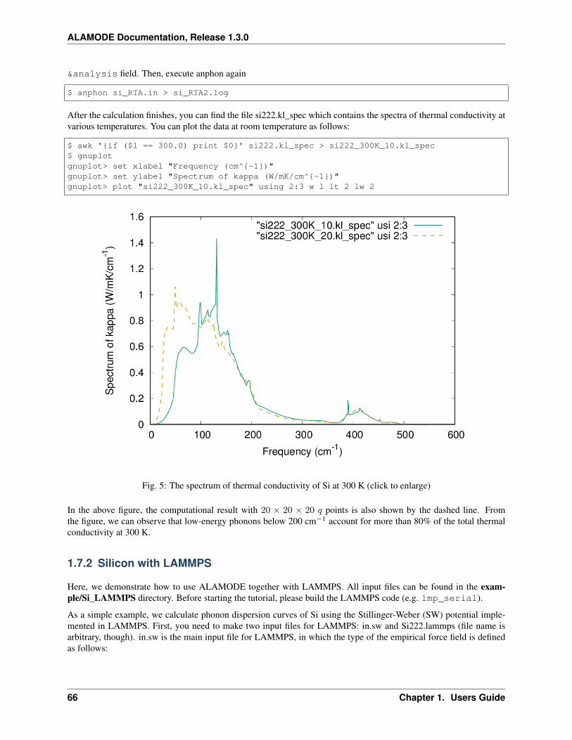
ALAMODE Documentation, Release 1.3.0
&analysis field. Then, execute anphon again
$ anphon si_RTA.in > si_RTA2.log
After the calculation finishes, you can find the file si222.kl_spec which contains the spectra of thermal conductivity atvarious temperatures. You can plot the data at room temperature as follows:
$ awk 'if ($1 == 300.0) print $0' si222.kl_spec > si222_300K_10.kl_spec$ gnuplotgnuplot> set xlabel "Frequency (cm^-1)"gnuplot> set ylabel "Spectrum of kappa (W/mK/cm^-1)"gnuplot> plot "si222_300K_10.kl_spec" using 2:3 w l lt 2 lw 2
Fig. 5: The spectrum of thermal conductivity of Si at 300 K (click to enlarge)
In the above figure, the computational result with 20 × 20 × 20 𝑞 points is also shown by the dashed line. Fromthe figure, we can observe that low-energy phonons below 200 cm−1 account for more than 80% of the total thermalconductivity at 300 K.
1.7.2 Silicon with LAMMPS
Here, we demonstrate how to use ALAMODE together with LAMMPS. All input files can be found in the exam-ple/Si_LAMMPS directory. Before starting the tutorial, please build the LAMMPS code (e.g. lmp_serial).
As a simple example, we calculate phonon dispersion curves of Si using the Stillinger-Weber (SW) potential imple-mented in LAMMPS. First, you need to make two input files for LAMMPS: in.sw and Si222.lammps (file name isarbitrary, though). in.sw is the main input file for LAMMPS, in which the type of the empirical force field is definedas follows:
66 Chapter 1. Users Guide

ALAMODE Documentation, Release 1.3.0
units metalatom_style atomicboundary p p p
read_data tmp.lammps
pair_style swpair_coeff * * Si.sw Si
dump 1 all custom 1 XFSET id xu yu zu fx fy fzdump_modify 1 format float "%20.15f"run 0
In the file Si222.lammps, the lattice vectors and atomic positions of a relaxed supercell structure are defined as follows:
# Structure data of Si (2x2x2 conventional)
64 atoms1 atom types
0.000000 10.800000 xlo xhi0.000000 10.800000 ylo yhi0.000000 10.800000 zlo zhi0.000000 0.000000 0.000000 xy xz yz
Masses
1 28.085
Atoms
1 1 0.000000 0.000000 0.0000002 1 0.000000 0.000000 5.4000003 1 0.000000 2.700000 2.7000004 1 0.000000 2.700000 8.1000005 1 0.000000 5.400000 0.0000006 1 0.000000 5.400000 5.4000007 1 0.000000 8.100000 2.7000008 1 0.000000 8.100000 8.1000009 1 1.350000 1.350000 1.35000010 1 1.350000 1.350000 6.75000011 1 1.350000 4.050000 4.05000012 1 1.350000 4.050000 9.45000013 1 1.350000 6.750000 1.35000014 1 1.350000 6.750000 6.750000
Next, please generate a set of structure files for displaced configurations using the python script:
$ python displace.py --LAMMPS=Si222.lammps --mag=0.01 --prefix harm -pf si222.→˓pattern_HARMONIC$ python displace.py --LAMMPS=Si222.lammps --mag=0.04 --prefix cubic -pf si222.→˓pattern_ANHARM3
The pattern files can be generated by the alm code as decribed here. The above commands create harm1.lammpsand cubic[01-20].lammps structure files. Then, run the following script and calculate atomic forces for thegenerated structures. This should finish in a few seconds.
1.7. Tutorial 67
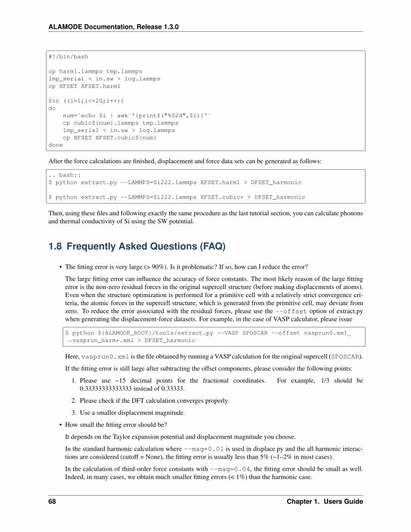
ALAMODE Documentation, Release 1.3.0
#!/bin/bash
cp harm1.lammps tmp.lammpslmp_serial < in.sw > log.lammpscp XFSET XFSET.harm1
for ((i=1;i<=20;i++))do
num=`echo $i | awk 'printf("%02d",$1)'`cp cubic$num.lammps tmp.lammpslmp_serial < in.sw > log.lammpscp XFSET XFSET.cubic$num
done
After the force calculations are finished, displacement and force data sets can be generated as follows:
.. bash::$ python extract.py --LAMMPS=Si222.lammps XFSET.harm1 > DFSET_harmonic
$ python extract.py --LAMMPS=Si222.lammps XFSET.cubic* > DFSET_harmonic
Then, using these files and following exactly the same procedure as the last tutorial section, you can calculate phononsand thermal conductivity of Si using the SW potential.
1.8 Frequently Asked Questions (FAQ)
• The fitting error is very large (> 90%). Is it problematic? If so, how can I reduce the error?
The large fitting error can influence the accuracy of force constants. The most likely reason of the large fittingerror is the non-zero residual forces in the original supercell structure (before making displacements of atoms).Even when the structure optimization is performed for a primitive cell with a relatively strict convergence cri-teria, the atomic forces in the supercell structure, which is generated from the primitive cell, may deviate fromzero. To reduce the error associated with the residual forces, please use the --offset option of extract.pywhen generating the displacement-force datasets. For example, in the case of VASP calculator, please issue
$ python $ALAMODE_ROOT/tools/extract.py --VASP SPOSCAR --offset vasprun0.xml→˓vasprun_harm*.xml > DFSET_harmonic
Here, vasprun0.xml is the file obtained by running a VASP calculation for the original supercell (SPOSCAR).
If the fitting error is still large after subtracting the offset components, please consider the following points:
1. Please use ~15 decimal points for the fractional coordinates. For example, 1/3 should be0.33333333333333 instead of 0.33333.
2. Please check if the DFT calculation converges properly.
3. Use a smaller displacement magnitude.
• How small the fitting error should be?
It depends on the Taylor expansion potential and displacement magnitude you choose.
In the standard harmonic calculation where --mag=0.01 is used in displace.py and the all harmonic interac-tions are considered (cutoff = None), the fitting error is usually less than 5% (~1–2% in most cases).
In the calculation of third-order force constants with --mag=0.04, the fitting error should be small as well.Indeed, in many cases, we obtain much smaller fitting errors (< 1%) than the harmonic case.
68 Chapter 1. Users Guide
ALAMODE Documentation, Release 1.3.0
In the temperature-dependent effective potential method, we try to fit the harmonic potential to the displacement-force datasets sampled by ab initio molecular dynamics at finite temperature. Therefore, the fitting error tendsto be much larger (> 10%).
• What value should I use for the cutoff radius?
For the harmonic term, I would recommend using “None”, which considers all harmonic interactions inside thesupercell. This choice does not increase the computational costs that much because the number of displacementpatterns does not change. Also, the harmonic dynamical matrix becomes exact at the commensurate q pointsonly when the “None” option is selected. (Giving a very large cutoff radius has the same effect as giving“None”.)
For the anharmonic terms, you will need to increase the cutoff radii gradually and check the convergence ofphysical quantities, such as thermal conductivity and free energy, with respect to the cutoff values. In mostcases, the cutoff radius of 10 Bohr is a good guess, but you may need to use a larger value for polar materials.So be careful.
• Why are the phonon dispersion curves discontinuous at the Brillouin zone boundaries?
Probably, you are wrongly using the supercell lattice vectors for the &cell field of the anphon code. If so,please use the primitive lattice vectors for anphon.
Note: For the &cell field of alm, you need to give the supercell lattice vectors.
1.8. Frequently Asked Questions (FAQ) 69

ALAMODE Documentation, Release 1.3.0
70 Chapter 1. Users Guide

CHAPTER 2
Indices and tables
• genindex
• modindex
• search
71