alan turing’s morphogenesis: on the wonders of...
TRANSCRIPT

UNIVERSITY OF MANCHESTER
SCHOOL OF COMPUTER SCIENCE
THIRD YEAR PROJECT
Alan Turing’s morphogenesis: on thewonders of nature
Author:Vasilis NICOLAOU
Degree Programme:MEng(Hons) Software Engineering
Supervisor:Dr. Eva M. NAVARRO-LOPEZ
April 2013

Abstract
Alan Turing in 1952 described mathematically how cells can self-organise to form a varietyof structures. He called this phenomenon morphogenesis, which means the creation of shape.Cells communicate with each other by diffusion, a process where chemical compounds or mor-phogens move from higher to lower concentrations. The project studies various aspects ofmorphogenesis and analyses several reaction-diffusion mathematical models. The main goalwas to translate the simulations of such dynamical systems into descriptive animations of theprocesses involved. The project exploits morphogenesis exploring the phenomenon of cellmutation. Producing sound from reaction-diffusion mathematical models is also introduced.Finally, the project proposes applications of morphogenesis in engineering achieving the merg-ing of the separate worlds of biology, mathematics, computer science, engineering and arts.
Title of project: Alan Turing’s morphogenesis: on the wonders of nature.
Author: Vasilis Nicolaou
Supervisor: Eva M. Navarro Lopez
April 2013

Acknowledgements
I would like to thank my supervisor, Dr. Eva M. Navarro Lopez, for her academic wisdom, hercaring manner and her constant help throughout the year which was essential for completingthis project.
I also thank my friends and co-students for the funny moments and inspirational conversa-tions throughout a challenging and difficult year.
Last but not least, I thank my family for believing and supporting me throughout my Uni-versity studies.

Contents
List of Figures iii
List of Tables v
1 Introduction 11.1 Morphogenesis . . . . . . . . . . . . . . . . . . . . . . . . . . . . . . . . . . 11.2 Project objectives . . . . . . . . . . . . . . . . . . . . . . . . . . . . . . . . . 11.3 Background . . . . . . . . . . . . . . . . . . . . . . . . . . . . . . . . . . . . 21.4 Approach . . . . . . . . . . . . . . . . . . . . . . . . . . . . . . . . . . . . . 21.5 Summary of results . . . . . . . . . . . . . . . . . . . . . . . . . . . . . . . . 31.6 Report structure . . . . . . . . . . . . . . . . . . . . . . . . . . . . . . . . . . 3
2 Biochemical concepts 52.1 Chemical reactions . . . . . . . . . . . . . . . . . . . . . . . . . . . . . . . . 52.2 Cell diffusion . . . . . . . . . . . . . . . . . . . . . . . . . . . . . . . . . . . 6
3 Mathematical concepts 83.1 Dynamical systems . . . . . . . . . . . . . . . . . . . . . . . . . . . . . . . . 8
3.1.1 Non-linear systems . . . . . . . . . . . . . . . . . . . . . . . . . . . . 93.1.2 Linear systems . . . . . . . . . . . . . . . . . . . . . . . . . . . . . . 10
3.2 Numerical stability . . . . . . . . . . . . . . . . . . . . . . . . . . . . . . . . 12
4 Models of morphogenesis 144.1 The Gray-Scott model . . . . . . . . . . . . . . . . . . . . . . . . . . . . . . . 144.2 The L-Systems equations . . . . . . . . . . . . . . . . . . . . . . . . . . . . . 154.3 The Gizburg-Landau model . . . . . . . . . . . . . . . . . . . . . . . . . . . . 16
5 Software development tools and concepts 175.1 Matlab . . . . . . . . . . . . . . . . . . . . . . . . . . . . . . . . . . . . . . . 17
5.1.1 Modelling morphogenesis . . . . . . . . . . . . . . . . . . . . . . . . 185.1.2 Integrating ordinary differential equations . . . . . . . . . . . . . . . . 185.1.3 Plotting the results . . . . . . . . . . . . . . . . . . . . . . . . . . . . 195.1.4 Creating movies . . . . . . . . . . . . . . . . . . . . . . . . . . . . . 205.1.5 Producing sound . . . . . . . . . . . . . . . . . . . . . . . . . . . . . 21
5.2 Java . . . . . . . . . . . . . . . . . . . . . . . . . . . . . . . . . . . . . . . . 225.2.1 Implementing Euler’s method . . . . . . . . . . . . . . . . . . . . . . 225.2.2 Process management . . . . . . . . . . . . . . . . . . . . . . . . . . . 235.2.3 The scheduling problem . . . . . . . . . . . . . . . . . . . . . . . . . 25
i

CONTENTS CONTENTS
6 Applications and results 296.1 Chemical reactions . . . . . . . . . . . . . . . . . . . . . . . . . . . . . . . . 296.2 Diffusion . . . . . . . . . . . . . . . . . . . . . . . . . . . . . . . . . . . . . 326.3 Reaction-diffusion . . . . . . . . . . . . . . . . . . . . . . . . . . . . . . . . 35
6.3.1 Implementing and testing with linearised models . . . . . . . . . . . . 356.3.2 Non-linear models . . . . . . . . . . . . . . . . . . . . . . . . . . . . 396.3.3 Introducing mutation . . . . . . . . . . . . . . . . . . . . . . . . . . . 39
6.4 Producing sound . . . . . . . . . . . . . . . . . . . . . . . . . . . . . . . . . 446.5 Comparing schedulers . . . . . . . . . . . . . . . . . . . . . . . . . . . . . . 44
7 Software development 487.1 Model simulations . . . . . . . . . . . . . . . . . . . . . . . . . . . . . . . . 48
7.1.1 Code structure . . . . . . . . . . . . . . . . . . . . . . . . . . . . . . 487.1.2 Testing . . . . . . . . . . . . . . . . . . . . . . . . . . . . . . . . . . 487.1.3 Documentation . . . . . . . . . . . . . . . . . . . . . . . . . . . . . . 49
7.2 Process scheduling . . . . . . . . . . . . . . . . . . . . . . . . . . . . . . . . 497.2.1 Methodology . . . . . . . . . . . . . . . . . . . . . . . . . . . . . . . 497.2.2 Code structure . . . . . . . . . . . . . . . . . . . . . . . . . . . . . . 497.2.3 Testing . . . . . . . . . . . . . . . . . . . . . . . . . . . . . . . . . . 50
7.3 Scripts and tools . . . . . . . . . . . . . . . . . . . . . . . . . . . . . . . . . . 50
8 Conclusion 52
Bibliography 54
Appendices 56
A Matlab programs 57A.1 Template reaction diffusion model.m . . . . . . . . . . . . . . . . . . . . . . 57A.2 Template playMovie.m . . . . . . . . . . . . . . . . . . . . . . . . . . . . . . 58A.3 Template initialiseA.m . . . . . . . . . . . . . . . . . . . . . . . . . . . . . . 58
B Java programs 59B.1 AbstractFunction.java . . . . . . . . . . . . . . . . . . . . . . . . . . . . . . . 59B.2 ODE.java . . . . . . . . . . . . . . . . . . . . . . . . . . . . . . . . . . . . . 60B.3 AbstractODE.java . . . . . . . . . . . . . . . . . . . . . . . . . . . . . . . . . 60B.4 Scheduler.java . . . . . . . . . . . . . . . . . . . . . . . . . . . . . . . . . . . 61B.5 Process.java . . . . . . . . . . . . . . . . . . . . . . . . . . . . . . . . . . . . 62
C Bash scripts and gnuplot scripts 64C.1 matdoc . . . . . . . . . . . . . . . . . . . . . . . . . . . . . . . . . . . . . . . 64C.2 matdoc pages . . . . . . . . . . . . . . . . . . . . . . . . . . . . . . . . . . . 64C.3 totalTime.p . . . . . . . . . . . . . . . . . . . . . . . . . . . . . . . . . . . . 64C.4 run-test . . . . . . . . . . . . . . . . . . . . . . . . . . . . . . . . . . . . . . 65C.5 run-tests . . . . . . . . . . . . . . . . . . . . . . . . . . . . . . . . . . . . . . 65
ii

List of Figures
2.1 Interconnection of cells in a ring-shaped structure. . . . . . . . . . . . . . . . . 72.2 2-dimensional surface wrapped in a torus-shaped structure. . . . . . . . . . . . 7
5.1 An image representation of the structure produced by a system of cells. . . . . 185.2 Template of Matlab code for solving ODE’s. . . . . . . . . . . . . . . . . . . . 195.3 Graph presenting data from Table 5.1 , Time×X . . . . . . . . . . . . . . . . . 205.4 Scheme of a process as handled by the implementation of the process manage-
ment framework. . . . . . . . . . . . . . . . . . . . . . . . . . . . . . . . . . 24
6.1 Graph showing the behaviour of the chemical reaction when there is a balancein all rates (experiment 1,Table 6.1). . . . . . . . . . . . . . . . . . . . . . . . 30
6.2 Graph showing how a higher rate of C breaking into X affects Michaelis-Menten mechanism (experiment 2, Table 6.1). . . . . . . . . . . . . . . . . . . 31
6.3 Graph showing how a higher rate of C producing product P affects the Michaelis-Menten mechanism (experiment 3, Table 6.1). . . . . . . . . . . . . . . . . . . 31
6.4 Graph showing how a higher rate of producing C affects the Michaelis-Mentenmechanism (experiment 4, Table 6.1). . . . . . . . . . . . . . . . . . . . . . . 32
6.5 Graph showing chemical concentrations during the diffusion process (experi-ment 1, Table 6.2). . . . . . . . . . . . . . . . . . . . . . . . . . . . . . . . . 33
6.6 Graph showing how the size of the cells affects the diffusion process (experi-ment 2, Table 6.2). . . . . . . . . . . . . . . . . . . . . . . . . . . . . . . . . 34
6.7 Graph showing how the number of the cells affects the diffusion process (ex-periment 3, Table 6.2). . . . . . . . . . . . . . . . . . . . . . . . . . . . . . . 34
6.8 Graph showing the diffusion process in a torus structure (experiment 4, Table6.2). . . . . . . . . . . . . . . . . . . . . . . . . . . . . . . . . . . . . . . . . 35
6.9 Graph showing the behaviour of a linear reaction-diffusion system (experiment1, Table 6.3). . . . . . . . . . . . . . . . . . . . . . . . . . . . . . . . . . . . 37
6.10 Graph showing the behaviour of a linear reaction-diffusion system with differ-ent values of the Jacobian matrix (experiment 2, Table 6.3). . . . . . . . . . . . 37
6.11 Graph showing that a linearised reaction-diffusion system is unstable if stabilityconditions are not satisfied (experiment 3 from Table 6.3). . . . . . . . . . . . 38
6.12 Graph showing the same linear system as in experiment 1 but without diffusion(experiment 4, Table 6.3). . . . . . . . . . . . . . . . . . . . . . . . . . . . . . 38
6.13 Graph showing how the behaviour of the linear system differantiates with largediffusion coefficients (experiment 2, Table 6.4 opposed to experiment 1, Figure6.9). . . . . . . . . . . . . . . . . . . . . . . . . . . . . . . . . . . . . . . . . 40
iii

LIST OF FIGURES LIST OF FIGURES
6.14 Graph showing how the behaviour of the linear system differantiates with verylarge diffusion coefficients (experiment 4, Table 6.4 opposed to experiment 3,figure 6.10). . . . . . . . . . . . . . . . . . . . . . . . . . . . . . . . . . . . . 40
6.15 Initial, middle and final snapshots of the structure of the L-systems of experi-ment No. 1, Table 6.5. . . . . . . . . . . . . . . . . . . . . . . . . . . . . . . 41
6.16 Initial, middle and final snapshots of the structure of the L-systems with morecells as shown in experiment 2, Table 6.5. . . . . . . . . . . . . . . . . . . . . 41
6.17 Initial, middle and final snapshots of the structure of the L-systems with differ-ent diffusion coefficients (experiment 3, Table 6.5). . . . . . . . . . . . . . . . 41
6.18 Initial, middle and final snapshots of the structure of the L-systems with differ-ent diffusion coefficients (experiment 4, Table 6.5). . . . . . . . . . . . . . . . 42
6.19 Initial, middle and final snapshots of the structure of the Gray-Scott model withparameters shown in experiment No.5, Table 6.5. . . . . . . . . . . . . . . . . 42
6.20 Initial, middle and final snapshots of the structure of the Gray-Scott model withdifferent reaction rates (experiment No.5, Table 6.5). . . . . . . . . . . . . . . 42
6.21 Initial state, final structure before mutation , and recovered structure after mu-tation with mutation probability 0.001 (experiment 1, Table 6.6). . . . . . . . . 43
6.22 Initial state, final structure before and after mutation showing that with proba-bility 0.01 the structure changes (experiment 2, Table 6.6). . . . . . . . . . . . 43
6.23 Pattern produced by the Gizburg-Landau model. . . . . . . . . . . . . . . . . . 446.24 Sound spectra by calculating the mean values of the morphogens. . . . . . . . . 456.25 Comparison of the scheduler implementations with 100 processes in the queue
(experiment No. 1 of Table 6.7). . . . . . . . . . . . . . . . . . . . . . . . . . 466.26 Comparison of the scheduler implementations with 1000 processes in the queue
(experiment No. 2 of Table 6.7). . . . . . . . . . . . . . . . . . . . . . . . . . 466.27 Comparison of the scheduler implementations with 1000 processes in the queue
and a different diffusion coefficient (5) for the diffusion-inspired scheduler (ex-periment No. 3 of Table 6.7). . . . . . . . . . . . . . . . . . . . . . . . . . . . 47
6.28 Comparison of the scheduler implementations with 1000 processes in the queueand the diffusion coefficient of the diffusion-inspired scheduler being 15 (ex-periment No. 4 of Table 6.7). . . . . . . . . . . . . . . . . . . . . . . . . . . . 47
iv

List of Tables
3.1 Mathematical representation of biological elements. . . . . . . . . . . . . . . . 8
5.1 Data as obtained from integrating a function with input array X of size 4×sizeOf(t). . . . . . . . . . . . . . . . . . . . . . . . . . . . . . . . . . . . . 20
6.1 Parameters used by solving the chemical equation (6.1). . . . . . . . . . . . . . 306.2 Parameters used to run tests on diffusion. . . . . . . . . . . . . . . . . . . . . 336.3 Experiments using the Jacobian matrix and diffusion for modelling the process
of reaction-diffusion in a ring of cells. . . . . . . . . . . . . . . . . . . . . . . 366.4 Experiments on how a linear system is affected from diffusion. . . . . . . . . . 396.5 Experiments of non-linear models with various parameters. . . . . . . . . . . . 416.6 Showing the effect of mutation on different probabilities. . . . . . . . . . . . . 436.7 Experiment parameters for testing the diffusion-inspired scheduler against other
schedulers. . . . . . . . . . . . . . . . . . . . . . . . . . . . . . . . . . . . . 45
7.1 Description of the implemented scripts that automate documentation and testing. 51
v

List of Algorithms
1 Colour mapping . . . . . . . . . . . . . . . . . . . . . . . . . . . . . . . . . . 212 Euler’s method . . . . . . . . . . . . . . . . . . . . . . . . . . . . . . . . . . 233 Random scheduler . . . . . . . . . . . . . . . . . . . . . . . . . . . . . . . . 264 Round Robin scheduler . . . . . . . . . . . . . . . . . . . . . . . . . . . . . . 265 Priority scheduler . . . . . . . . . . . . . . . . . . . . . . . . . . . . . . . . . 276 Diffusion-inspired scheduler . . . . . . . . . . . . . . . . . . . . . . . . . . . 28
vi
Chapter 1
Introduction
1.1 MorphogenesisMorphogenesis is the biological process that defines how a system of cells is organised andshaped. The word originates from the Greek words ‘morf ’ which means shape and ‘gènesic’which means birth. Alan Turing in his paper ‘The chemical basis of morphogenesis’ gives amathematical model that can approximate how an embryo develops its various organs [1].
The challenge was to show how from a single cell that replicates into identical cells, var-ious organs are developed with different functionalities. For example, in a human embryo,there is initially a single cell that was produced from half the characteristics of the mother andhalf of the father. Eventually, millions of cells are generated. Nevertheless, they manage todifferentiate into groups that form parts of different organs.
Turing defined a hypothetical chemical substance called morphogen. A morphogen is anabstract term which represents a chemical compound that gives the cell certain properties ac-cording to its concentration. A cell, therefore, may be defined as a vector of morphogens thatreact together forming the state of a cell. In addition, each cell has several neighbouring/adja-cent cells.
When cells with different concentrations of chemical compounds are connected, the phe-nomenon of diffusion is observed. The membrane of a cell has a property that allows chemicalsubstances to move from higher to lower concentrations. This is how cells communicate. Dif-fusion is further explained in Section 2.2.
By constructing mathematical equations that approximate chemical reactions and diffusion,one can define models that approximate the phenomenon of morphogenesis. Such models aredescribed in Chapter 4.
1.2 Project objectivesThis project studies the idea of morphogenesis that Alan Turing proposed and subsequentlyproduces software applications that simulate various models of the reaction-diffusion biologicalprocess. The simulations combine graphs that may be used for analysis or testing and movies1
that show how cells are organised forming structural patterns. Simulations also visualise theeffects of cell mutations, processed as random changes in morphogen concentrations after asystem develops a structured shape.
1Movies are available at: http://www.youtube.com/watch?v=2JppD_Mw_3k
1 of 65

1.3. BACKGROUND CHAPTER 1. INTRODUCTION
The project goes a step further and introduces applications of morphogenesis in engineer-ing. A process scheduling algorithm inspired by the reaction-diffusion concept has been de-veloped and compared to traditional schedulers such as the Round Robin. The idea of how ascheduler is related to morphogenesis is not obvious and is described in section 5.2.3.
Some experiments study the possibility of producing sound by the use of mathematicalmodels that produce continuous oscillations. Due time limitations, experiments are not exten-sive and no meaningful sound output was produced. However, readers and future researchesof the subject are encouraged into further study of such experiments, since graphs present abehaviour similar to sound waves.
1.3 BackgroundMorphogenesis is defined by Alan Turing as the process of how cells of an embryo create shapeout of an initially chaotic behaviour [1]. Cells are interacting with each other by diffusingchemical substances which in Turing’s morphogenesis model are defined as morphogens. Theterm morphogen is abstract and should not be confused with DNA genes, chromosomes orcertain chemical elements. A morphogen is considered to be a chemical substance that hassome theoretical properties which give to cell specific characteristics. Morphogens may alsoreact with each other in the same way chemical molecules do. Reactions and diffusion happenover time and thus morphogenesis process can be a dynamical system. Thus, it can be modelledmathematically using differential equations, by suggesting that each cell has a state accordingto its morphogen concentrations and that state is subject to change over time.
The approach followed for simulation and analysis of morphogenesis’ models uses a varietyof concepts of the mathematical, biochemical and programming domain. Such concepts arediscussed in this report providing the knowledge basis that is necessary for the reader to followthe approach and the implementation procedure of the project.
Finally, various papers and articles [2][3][4] that study the phenomenon of morphogenesisand pattern generation were used to identify mathematical models of the reaction-diffusionprocess and were the spark for further exploration of ideas related to morphogenesis.
1.4 ApproachThe approach was partitioned in several stages. Since the project has a strong mathematicalcomponent, background knowledge of the mathematical concepts that were involved are pre-sented. The information on the mathematical knowledge that is required is given by Alan Tur-ing in his paper [1]. To sum up, this subject merges ordinary differential equations, integrationmethods, algebra and computational theory.
Application of mathematical concepts from dynamical systems theory is required to buildan understanding on how software applications of mathematical models are developed. Sincethe main tool to implement such models was Matlab, suitable software design methodologieswere identified to facilitate a concrete development of the software applications.
An agile development methodology was followed [5]. A basic application was built atan early stage. This enabled concurrency in researching and programming which resulted inidentifying and implementing features, re-factoring code and fixing bugs, achieving the im-plementation of the variety of applications to be well defined, maintainable and reasonablydocumented.
2 of 65

1.5. SUMMARY OF RESULTS CHAPTER 1. INTRODUCTION
In brief, the project is researched based, involving various concepts from chemistry, bi-ology, mathematics and software design. The absence of requirement gathering from usersenabled the intense research and tutorial discussions to embrace the study of various ideas thatwere presented throughout the life-cycle of the project.
1.5 Summary of resultsResults are separated into categories according to the purpose of each application. Informationabout chemical reactions and diffusion is provided. The data from the applications and exper-iments that took place are discussed. After that, various mathematical models are simulatedfor studying their parameters and how the latter affect their behaviour. Finally, experimentalideas that involve cell mutation, sound producing and process scheduling using diffusion areintroduced.
The presentation of results shows at which circumstances cells form structures and how dif-ferent shapes are produced by altering the parameters of a model or by using different models.Furthermore, perturbations are introduced in the form of cell mutations and explore whetherthe structure of the system is altered. Finally, the possibility of producing sound is introducedalong with a study on how morphogenesis might be applied in computer science as a natureinspired algorithm.
1.6 Report structureThe report consists of three parts.
1. The background information for the reader to build the basic concepts involved in thisproject.
2. The applications that were implemented and the results obtained in each stage of theproject.
3. The development process and methodologies that were followed to build the softwareartifacts. Thus, offering a point of reference to the reader for building extensions orsimilar solutions.
The main morphogenesis models are supplied in Chapter 4. Those are the L-systems equa-tions, the Gray-Scott model and the Gizburg-Landau model. The background information pro-vides all the necessary knowledge on the concepts that are studied by the project. The mathe-matical background is the most important and advanced topic, since all the biochemical relatedissues, such as the chemical reactions and cell diffusion are described by differential equations.Thus, Chapter 2 consists of basic information about how chemical compounds react and whatassumptions are made for both chemical reactions and diffusion when defining a mathematicalmodel that approximates such behaviours. Finally, the programming background is given, withinformation on Matlab and Java, including key features of each language and pseudo-code ofthe algorithms that were implemented.
The development process that is discussed in Chapter 5 gives the methodology used to im-plement each software application and help in reading the code for the purpose of maintainingor expanding it. It also includes information about testing and visualising data by using script
3 of 65

1.6. REPORT STRUCTURE CHAPTER 1. INTRODUCTION
languages that enable automation and minimise the amount of time spent by combining plottingand testing.
Results are given in Chapter 6 and are presented in a way that reflects the progress of theproject, starting from the study of chemical reactions and cell diffusion and then progressingto complete mathematical models of morphogenesis. At the end, the results of experimentingwith process management combined with morphogenesis are supplied. Results include imagesthat show snapshots of how the reaction-diffusion process evolves in time. Graphs showing thenumerical state of a system or statistics about comparison of algorithms are also given.
Finally, the appendices contain the important code implementations of the project. Sincevarious papers on morphogenesis [3][4] contain examples of their code artifacts, it is importantthat alternative solutions are given.
4 of 65

Chapter 2
Biochemical concepts
An elementary level of knowledge in chemistry is needed to understand the concepts that arediscussed in this report. As mentioned previously, the reactions do not include real chemicalelements, but rather some abstract compounds called morphogens. The process however, is thesame as when real chemical elements react. This enables the use of various reaction equationswith different rates and therefore different models, that widen the range of the experiments inorder to approximate physical systems.
2.1 Chemical reactionsA reaction is defined as the interaction of a set of two or more chemical compounds to produceanother, different set of one or more chemical compounds. The equation to describe such aprocess is:
X +Y →r
Z (2.1)
Equation (2.1) means, that the chemical compound X is reacting with the compound Yand both produce Z at a rate r. Thus, when one of the concentrations of either X or Y runsout, the reaction stops. From the chemical equation that describes a reaction, a mathematicaldescription may be constructed. Since reaction depends on time (the concentration of Z isincreased over time according to a rate r, X and Y concentrations are decreased at the samerate), a chemical reaction should be considered as a dynamical system. As described in section3.1 a dynamical system is defined by ordinary differential equations.
The system of equation (2.1) has 3 states, X, Y and Z. Therefore, three equations are neededto describe each state of the system in time. Z is produced at a rate r. In addition, concentrationsof X and Y that are decreased in the same rate (for instance, one unit of both X and Y is neededto produce one unit of Z). The equation that gives the state of Z at any time, is:
Z = rXYt +Z0 (2.2)
Likewise for X and Y with the main difference that those compounds are expended to produceZ, so the equations are:
X =−rXYt +X0 (2.3)
Y =−rXYt +Y0 (2.4)
Z0,X0 and Y0 are the initial concentrations of each chemical substance and r is the pa-rameter that represents the reaction rate. Differentiating equations (2.2), (2.3) and (2.4) the
5 of 65

2.2. CELL DIFFUSION CHAPTER 2. BIOCHEMICAL CONCEPTS
mathematical model is obtained as:dZdt
= rXY
dXdt
=−rXY
dYdt
=−rXY
2.2 Cell diffusionDiffusion is the process where chemical substances move from their higher to lower concen-trations. For example, if two cells A and B are attached, containing 10 units and 2 unitsrespectively of a chemical X, then the chemical compound X will move from A to B until thechemical concentrations are balanced (6 units each). Turing suggested in his paper that thediffusion occurs similarly with the conduction of heat [1, p. 40]. By replacing the conductionwith diffusion, Turing gave the equation of diffusion in a ring of cells [1, p. 47] from which ageneral equation of diffusion can be extracted as shown in equation (2.5). The latter helps inexperimenting with cells that have any number of cells attached to them.
F = δ2K.∗ (
A
∑i=a
xi−Nx j) (2.5)
Where:
• A is the set of cells that are directly attached to cell j,
• N is the size of A (the number of cells attached to j),
• j is a cell of the system under study and it does not exist in set A,
• xi is a vector that contains the concentration of the chemical substances in cell i,
• K is a vector which contains diffusion coefficients for each chemical substance,
• δ is the size of the sides of the cells.
The binary operation ‘.*’ means that the vector multiplication is pair-wise (adopted from Mat-lab semantics [11]). That is: (
ab
).∗(
cd
)=(
acbd
)Turing considers the scenario of cells connected in a ring communicating with diffusion.
That means that every cell is connected to another two cells as shown in Figure 2.1. Therefore,the equation becomes:
Fring = δ2 ∗K.∗ (xi−1−2xi + xi+1) (2.6)
Diffusion in a torus is also considered in order to tackle the problem that arises by workingon a surface structure. For instance, consider a 2-dimensional matrix. The cells on the edgesare connected with three other cells. If a cylinder connection is made, that leaves the top andbottom cells to be connected with only three other cells and all others to be connected withfour. The solution is to connect every cell on an edge with a cell in the other edge-end. This
6 of 65

2.2. CELL DIFFUSION CHAPTER 2. BIOCHEMICAL CONCEPTS
Figure 2.1: Interconnection of cells in a ring-shaped structure.
forms the shape of torus shown in Figure 2.2. Another advantage by the use of a torus structureis that it allows a straightforward way of converting a surface of cells into an image, since it iseasily representable by using 2-dimensional computer graphics.
Figure 2.2: 2-dimensional surface wrapped in a torus-shaped structure.
7 of 65

Chapter 3
Mathematical concepts
This chapter gives information about the mathematical concepts that were used during thisproject. A basic knowledge of ordinary differential equations (ODE’s) and matrix algebrais needed. Main concepts such as dynamical systems are explained. Linear and non-linearsystems are also discussed, including the linearisation technique.
3.1 Dynamical systemsA dynamical system gives a functional description of a solution which varies in time. Mathe-matically a dynamical system is a function f (t,x)∀t ∈ R and x ∈ E ⊂ Rn, that describes howpoints x ∈ E change with respect to time [8, p. 182].
A mathematical definition to the problem based on dynamical systems is needed in orderto construct the mathematical model that describes the behaviour of the phenomenon of Mor-phogenesis.
Morphogenesis is the process that gives shape to biological organisms. Mathematically abiological system may be defined as a set of cells which contain a set of morphogens. Thus, acell is defined as a vector containing real values that represent the morphogen concentrations.Therefore, the functional model will be defined as a matrix of N vectors of size M, where N isthe number of cells and M is the number of morphogens that each cell contains. This is shownin Table 3.1.
Table 3.1: Mathematical representation of biological elements.Biological element Mathematical Representation Mathematical
DefinitionMorphogen A real value variable that represents
the concentration of the morphogenX ∈ R
Cell Vector of size M equal to the num-ber of morphogens that it contains
x ∈ RM
Physical System A matrix of size N equal to thenumber of cells that contains M 1-dimensional vectors of real values
S ∈ RN×M
8 of 65

3.1. DYNAMICAL SYSTEMS CHAPTER 3. MATHEMATICAL CONCEPTS
3.1.1 Non-linear systemsThe purpose of a mathematical model is the aid to the study of physical systems. It shouldbe noted, that any mathematical model gives an approximate solution of the physical system itdescribes. Therefore, the accuracy of any mathematical model is measured by the closeness ofthat model to the behaviour of that physical system. Such models are constructed by a set ofnon-linear differential equations.
This project focuses on the study of known mathematical models by analysing and sim-ulating their behaviour. Thus, some concepts of ordinary differential equations, integrationalgorithms and numerical stability theory are required.
The format of non-linear functions studied in this project is:
dxdt
= F(x(t)) = F(x1, ...,xn)
Where:
• x is a vector of size n.
• n is the number of morphogens.
• F is a non-linear function.
Such systems approximate the internal chemical reactions in each cell. To have a completereaction-diffusion model, the diffusion equation is added to the non-linear equations. Then themathematical model becomes:
dxi
dt= F(xi(t)) = F(xi)+δ(
A
∑j=a
x j−Nxi) (3.1)
∀i ∈ Cells.The construction of the diffusion equation is described in Section 2.2.
Analysis
There are two basic ideas concerning the analysis of non-linear systems; stability and oscil-lation. Stability is associated with the behaviour of the system around the equilibrium points.The main interest is to penetrate the system with small or large perturbations at its equilib-rium points and observe if its state changes [9]. Such perturbations are introduced in the formof mutation by altering the morphogen concentrations with random values. Other mutationsof great interest involve altering the parameters or the diffusion coefficients in the models ofmorphogenesis.
In terms of oscillating, the aim is to detect if the system shows an oscillatory behaviour andanalyse what properties that oscillation has: periodic/aperiodic, frequency, amplitude and howlong does it take for the system to stop oscillating and reach an equilibrium state [9, p. 7].
Simulation
Simulation means that the mathematical model is integrated in time and the results are shownvisually. Graphs, bar charts and finally movies show a representation of how cells are organisedinto shaped structures by converting the morphogen concentrations into colours.
9 of 65

3.1. DYNAMICAL SYSTEMS CHAPTER 3. MATHEMATICAL CONCEPTS
The integration of such models is done by programming in Matlab and the Java program-ming language. In order to develop solutions -in respect to mathematical models- in Matlaband Java, knowledge of integration algorithms and numerical stability is required.
The goal of the simulations is not only to show graphically how the state of a systemchanges, but also to prove that cells create shapes and ordered structures out of a chaotic andrandom initial state, according to the mathematical model that describes such a system.
Summarising, the simulations result from the integration of ordinary differential equationsthat define the mathematical model under study and then converting the solution into humanunderstandable visualisations.
3.1.2 Linear systemsThis project also studies linear systems of ordinary differential equations of the form:
x = Ax = A
x1...
xn
where A ∈ Rn×n and x ∈ Rn.
In general, a linear system can be viewed as
x = F(x)
where F(x) is a linear function. The reason behind the transformation to x = Ax is to exploitthe properties of any linear function. Those are the superposition property
F(x+ y) = f (x)+ f (y)
and the homogeneityF(ax) = aF(x)
By substituting F(x) by Ax it is directly shown that those properties are satisfied since:
F(x) = Ax =
a11x1 + . . .+a1nxn...
an1x1 + . . .+annxn
=
a11x1...
an1x1
+ . . .+
a1nxn...
annxn
= c
a′11x1 + . . .+a′1nxn...
a′n1x1 + . . .+a′nnxn
Linearisation process
It is possible to approximate a non-linear system around its equilibrium points by exploitinga property that most non-linear systems have. That property states that in the neighbourhoodof equilibrium solutions, non-linear systems behave as the linear system that approximatesthem. This means that a similar behaviour may be retrieved (for example, oscillatory behaviourwith certain amplitude and frequency), but the numerical values do not represent the valuesthat the non-linear system would have at that certain points in time. For example, the resultsof linear systems in Section 6.3.1 show that there are negative values representing chemicalconcentrations. This is not a problem, since only the behaviour is studied when approximatinga system by linearisation.
10 of 65

3.1. DYNAMICAL SYSTEMS CHAPTER 3. MATHEMATICAL CONCEPTS
The equilibrium points of the system are the values of vector x∈Rn at which dxdt = 0. When
all the derivatives of a system are evaluated to 0 then the system is unable to change as timepasses, since the integration step will always add zero. Exceptions are not studied.
The linearisation technique process as given from Florin Diacu [10, p. 227] is:
1. Shift equilibrium points to the origin, and define new variables, such as:
u = x− x0
2. Substitute the variables of the system with the new variables u from step 1 and obtain theequations for (u1, . . . , un)T .
3. Define G as the new form of the vector field such that
u = G(u)
The origin is an equilibrium such that:
G(0) = 0
The partial-derivative matrix A is formed as:
A =
∂G1∂u1|u=0 . . . ∂G1
∂un|u=0
... . . . ...∂Gn∂u1|u=0 . . . ∂Gn
∂un|u=0
4. Apply the derivatives shown in the corresponding matrix A (step 3) in terms of ui.
Example Let the non-linear system be:
x1 = (x1−3)(x2−1) (3.2)
x2 = (x1 +2)(x2 +5) (3.3)
The first step is to find the equilibrium point where x1 = x2 = 0 . It is easily observable thatwith x1 =−2 and x2 = 1 then
x1 = x2 = 0 (3.4)
A linearised system can approximate the behaviour of a non-linear system near the equi-librium points in (3.4). Thus, an isolated equilibrium should be used to shift the equilibriumpoints to the origin.
To achieve this, define:u = x− x0 (3.5)
x0 being the equilibrium points of the system.Equation (3.5) is the general form to work with the two variables of the system. Applying
(3.5) on (3.2) and (3.3), the two shifting variables are obtained:
u1 = x1 +2 (3.6)
11 of 65

3.2. NUMERICAL STABILITY CHAPTER 3. MATHEMATICAL CONCEPTS
u2 = x2−1 (3.7)
Using (3.6) and (3.7) on (3.2) and (3.3) the new system with the altered coordinates isobtained:
u1 = x1 and u2 = x2 ⇐⇒
u1 =−5u2 +u1u2,
u2 = 6u1 +u1u2
with
G =(
u1u2
)Following the steps 3 and 4 of the linearisation technique, the real values of the correspond-
ing matrix A are computed:
A =
(∂G1∂u1|u=0
∂G1∂u2|u=0
∂G2∂u1|u=0
∂G2∂u2|u=0
)=
(∂(−5u2+u1u2)
∂u1|u=0
∂(−5u2+u1u2)∂u2
|u=0∂(6u1+u1u2)
∂u1|u=0
∂(6u1+u1u2)∂u2
|u=0
)⇒ A =
(0 −56 0
)The linearized system around (u1,u2) = (0,0) is u = Au, with
u =(
u1u2
)This system, approximates the behaviour of the non-linear system defined by the equations(3.2) and (3.3)
3.2 Numerical stabilityA system is numerically unstable when its state grows uncontrollably to infinity. Instabilitymay occur for three reasons.
1. The system is unstable.
2. The system is unstable for the particular initial conditions and parameters.
3. Integration flaws of the ODE solver show that the system is unstable when it is not.
The interest of this project lies on reasons 2 and 3. This is because the construction of amathematical model does not concern this project, and thus, already proposed mathematicalmodels are used.
Numerical stability is a very important aspect to consider when using an ODE solver al-gorithm. Depending on the stiffness of the differential equations, a decision for the length ofthe time step must be made. The decision of the time step is crucial when having oscillatingsystems. This is due to the fact that, if the time step is not small enough and the amplitudegrows with large errors on each step then the amplitude of that oscillation will grow to infinityresulting in an unstable system.
12 of 65

3.2. NUMERICAL STABILITY CHAPTER 3. MATHEMATICAL CONCEPTS
In order to have a better understanding of why it is important to decide on the right time-step, consider the following situation: Think of a labyrinth with arbitrary length paths and wallsof arbitrary width. Someone wants to pass through the labyrinth by making steps of arbitrarysize. After a step, he observes if he arrived at a wall-end. If the step is big, it could passmistakenly through a wall, without noticing (in a virtual world) or crash at it (in a real world).How should the decision be made about the right size of the step? The example here is of astep in space, but the problem is of the same nature: if the step is big, the solver will present awrong or unstable behaviour.
On the other hand, having a very small step, increases the time that an ODE solver needsto complete the integration. In the labyrinth example, doing the smallest possible step eachtime to avoid wall collision, will result in a correct solution, but the time complexity would behuge. A dynamic approach, however, introduces variations on the time steps. An algorithmthat changes the time step is called implicit and an algorithm that uses a constant time step iscalled explicit. Most Matlab ODE solvers use an implicit approach of the Runge-Kutta familyalgorithms [11], reducing the time-steps when, for example, oscillations have low amplitude.
The Java implementation uses the explicit implementation of the Euler method since therange of the numbers is known, as the time slices that are given to a process by a scheduler arefixed. In addition, float point underflows are avoided by comparing the time slice given to aprocess with the smallest execution time-step a process is allowed to make.
13 of 65

Chapter 4
Models of morphogenesis
This project studies already-known reaction-diffusion models to produce different patterns andexplore various ideas and concepts. The Gray-Scott model and the L-Systems equations arethe core of the visualisation applications. The applications integrate those models and then bymapping the computed values into colours, images are generated and show the process of thecells producing a wide variety of structures.
4.1 The Gray-Scott modelThe Gray-Scott model describes a reaction-diffusion system [6]. The original model involvespartial derivatives and is given by the two partial differential equations:
u = du5u−uv2 +F(1−u),
v = dv5 v+uv2− (F + k)v (4.1)
Where:
• u and v represent the morphogen concentrations.
• du and dv are the diffusion coefficients of the morphogens u and v respectively.
• F and k are real constant values which represent the reaction rate.
• 5 is the laplacian operator of u for calculating diffusion in Euclidian space [3].
The analysis given by Benjamin M. Heineike in [3] finds several parameter ranges andvalues to produce several patterns. The equations were modified for the purposes of this project;the laplacian of the concentrations in respect to space was substituted by a linear diffusionequation as described in Section 2.2. Reaction functionsremain exactly the same as defined byGray-Scott in equations (4.1).
U +2V →F
3V,
V →F+k
P (4.2)
Thus, from equation (4.1), replacing the laplacian operator by the diffusion equation (2.5)the model becomes:
14 of 65

4.2. THE L-SYSTEMS EQUATIONS CHAPTER 4. MODELS OF MORPHOGENESIS
u j = du((A
∑i=a
ui−Nu j))−u jv2j +F(1−u j),
v j = dv(A
∑i=a
vi−Nv j)v+uv2− (F + k)v j, (4.3)
∀ j ∈Cells
Where:
• A is the set of adjacent cells to the current cell j.
• N is the number of elements of the set A.
If, for example, the structure of the cell interconnections is a ring then the equations (4.3)become:
ui = du(ule f to f (i)−2ui +urighto f (i))−uiv2i +F(1−ui),
vi = dv(vle f to f (i)−2vi + vrighto f (i))+uiv2i − (F + k)vi, (4.4)
∀i ∈Cells
The aim is to test the model with different parameters that were introduced by Benjamin M.Heineike [3] and discover if the Gray-Scott reaction function can be combined with diffusion,according to the conduction of heat as proposed by Alan Turing [1], to generate patterns. Theresults are presented in Section 6.3.2.
4.2 The L-Systems equationsThe L-Systems equations are proposed by Christopher G. Jennings [7]. His work involves aJava applet that generates patterns. Examples of such patterns involve cheetah skin patterns andfingerprints. The Java applet uses the explicit Euler’s method to integrate the reaction equationsand the diffusion. The reaction equations are:
u = uv−u−12,
v = 16−uv (4.5)
The same concepts were used and expanded into testing different ideas. The first idea wasto create patterns by applying different colour mappings and image processing techniques. Thesecond was to study how cell mutation can affect the normal structure of the system. Anotheraspect was to observe if the Euler’s method used in [7] was indeed accurate and what were thelimitations in terms of the produced patterns and the numerical computations.
Results are shown in paragraph 6.3.2 comparing the L-Systems equations to the Gray-Scottreaction function.
15 of 65
4.3. THE GIZBURG-LANDAU MODEL CHAPTER 4. MODELS OF MORPHOGENESIS
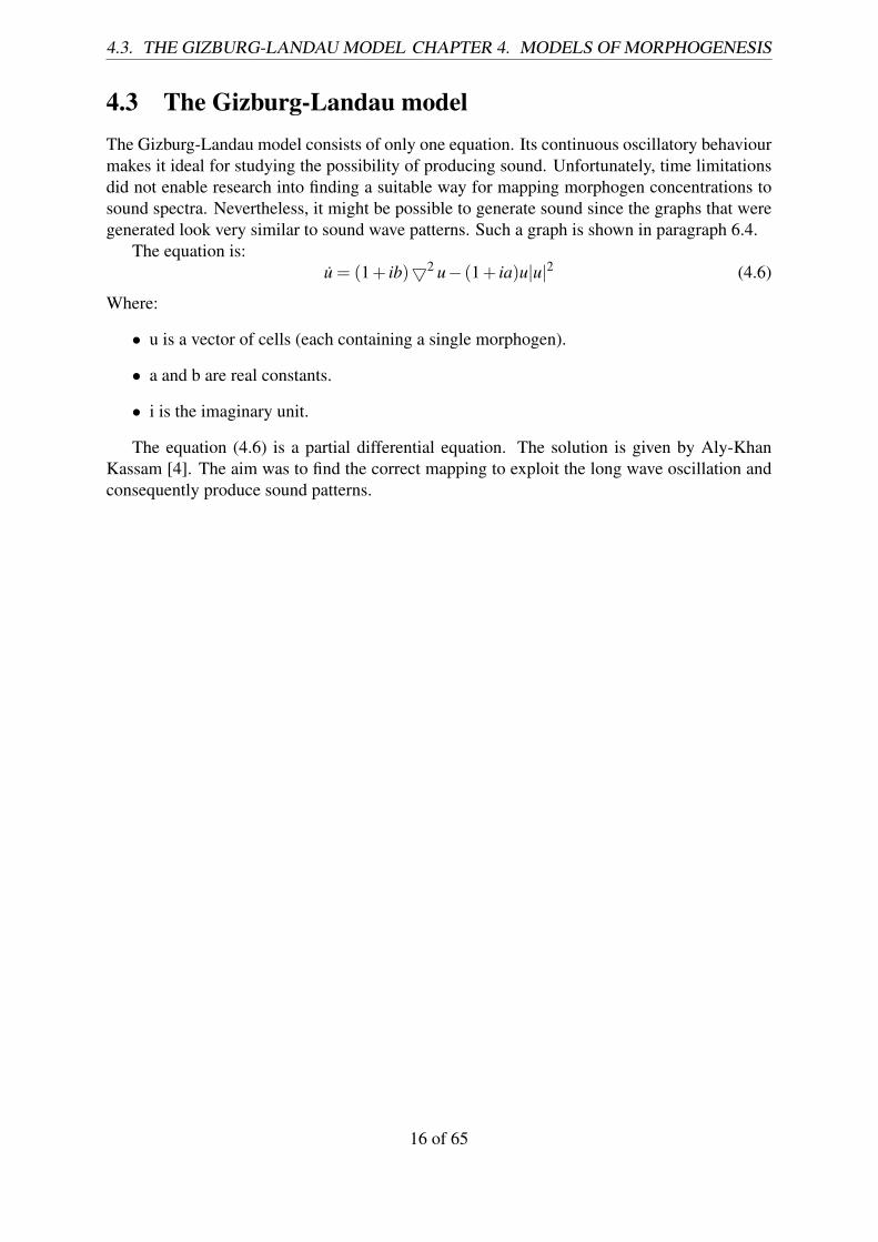
4.3 The Gizburg-Landau modelThe Gizburg-Landau model consists of only one equation. Its continuous oscillatory behaviourmakes it ideal for studying the possibility of producing sound. Unfortunately, time limitationsdid not enable research into finding a suitable way for mapping morphogen concentrations tosound spectra. Nevertheless, it might be possible to generate sound since the graphs that weregenerated look very similar to sound wave patterns. Such a graph is shown in paragraph 6.4.
The equation is:u = (1+ ib)52 u− (1+ ia)u|u|2 (4.6)
Where:
• u is a vector of cells (each containing a single morphogen).
• a and b are real constants.
• i is the imaginary unit.
The equation (4.6) is a partial differential equation. The solution is given by Aly-KhanKassam [4]. The aim was to find the correct mapping to exploit the long wave oscillation andconsequently produce sound patterns.
16 of 65

Chapter 5
Software development tools and concepts
The main deliverables of this project are two software artifacts.
1. A Matlab application that visualises the generation of patterns obtained from the inter-connections of cells.
2. An environment for testing process schedulers, including the implementation of a diffusion-inspired scheduler.
Various programming and script languages were used. The first application is written in Matlab.The second application includes two parts: a process management framework written in Javaon the Eclipse IDE and a set of bash scripts that use gnuplot [12] to generate bar graphs foranalysing and testing the various scheduler implementations. Basic knowledge of the concepts,the languages and the algorithms used are provided throughout this chapter.
5.1 MatlabMatlab is a programming environment developed by MathWorks [11]. It is ideal for workingwith vectors and matrices since it has build in matrix operations. It provides basic and advancedmathematical procedures and functions, such as sin, cos, Fourrier transformations and ordinarydifferential equation solvers. Its capability of producing all kinds of graphs and supplying aplethora of image processing functions makes it the ideal tool for studying the phenomenon ofmorphogenesis.
The approach was to study and test models by solving differential equations and producingrepresentational graphs and at the end, generating movies with image time frames to show howcells get organised and what shapes they produce. An example of such image frame is shownin Figure 5.1.
The functions in Matlab are written according to the format below:
f u n c t i o n <o u t p u t > = name(< arguments >)body
end
Note that the output can be a vector, a 2-dimensional array or an abstract structure, meaningthat the type of the output value will be given during the execution of the program.
17 of 65

5.1. MATLAB CHAPTER 5. SOFTWARE DEVELOPMENT TOOLS AND CONCEPTS
Figure 5.1: An image representation of the structure produced by a system of cells.
5.1.1 Modelling morphogenesisAs explained in Chapter 4, there are several dynamical models of the reaction-diffusion pro-cess in morphogenesis. The reaction model has the form x = F(x) and the diffusion model isaccording to conduction of heat as explained in paragraph 2.2 with cell interconnections of ringor torus-shaped structures. The Matlab program that was generated to solve such a model hastwo main parts.
The first part is the main function, where the initial conditions are given. Those conditionsare the number of cells, the initial concentrations of each chemical compound and the diffusioncoefficients. The main function constructs the data structures - which are vectors - and calls theappropriate ODE solver with arguments a function, a column vector (as the initial conditions)and a time span. Other arguments that are used by the ODE algorithm are explained in the nextparagraph. Any function can have inside the definition and implementation of another functionwhich is called a nested function.
The main purpose of the nested function is to make sure that the implementation of themathematical model is evaluated correctly. The equations of such a model should be imple-mented in the nested function in a way that the vector operations are evaluated correctly. Froma software development point of view, using a nested function instead of an external one isbetter, since the defined constants are easily shared from the main to its nested function. Anexample of a template code for solving ordinary differential equations is shown in Figure 5.2.
5.1.2 Integrating ordinary differential equationsMatlab provides a variety of ODE solver implementations each of them having different prop-erties. Note that there are some constraints in evaluating a model that describes fluid concentra-tions. The main constraint is that the concentrations must never get a negative value otherwisethe model will have no physical meaning.
The ODE-solver used in this project is the ode45. According to the Matlab documentationode45 is for solving non-stiff differential equations of medium order and it is the most commonused among the provided ode solvers [11].
Apart from the ODE arguments shown on line 5 in Figure 5.2, the solver can also be given
18 of 65

5.1. MATLAB CHAPTER 5. SOFTWARE DEVELOPMENT TOOLS AND CONCEPTS
f u n c t i o n o u t = f ( )%body , i n i t i a l i s e c o n s t a n t s%c a l l an ODE s o l v e r , such as ode45 , ode23 e t c . . .%example :[ t , x ] = ode45 ( @odefun , [0 1 0 0 ] ) ;%t h a t w i l l s o l v e e q u a t i o n s i n a t i m e span 0−100 s e c o n d s
p l o t x i n r e s p e c t t o t a s x ( t ( i ) ) = x ( i )
f u n c t i o n odefun = i n t e g r a t i o n ( t s p a n , i n i t )body e v a l u a t e e q u a t i o n sode = e q u a t i o n r e s u l t s ( column v e c t o r )
endend
Figure 5.2: Template of Matlab code for solving ODE’s.
a structure of options as an extra argument. Options are used to override any default behaviourand explicitly define the constraints that the solver must take into account. The options aredeclared with the use of the odeset function.
The odeset function takes an arbitrary length of arguments. First, a string value is givenwhich represents the key of the parameter that is intended to be overridden following by a realnumerical value. For example, any reaction-diffusion model requires that no cell has a negativeconcentration of any of its morphogens. Thus, the options are constructed with the code below:
options = odeset(′NonNegative′,(1 : N));
Where N is the size of the solution vector (cells×morphogens). Note that all matlab ode solversaccept a column vector as the initial conditions and thus extra care should be taken for convert-ing a 2-dimensional array to a column vector and the opposite correctly.
5.1.3 Plotting the resultsMatlab provides easy to use methods that make plotting graphs convenient. The interest lies onobserving graphically the equilibrium points of the system, how the system oscillates and forhow long. Thus, plotting the results helps in both the analysis of the system and the testing ofthe programs.
The plot function
The ODE solvers can plot a graph by default after the solution is calculated or in real time.However, it is better to store the results of the ODE solvers in arrays to have full control ofthe data. After executing an ODE solver two matrices can be retrieved; the time vector and anarray that can be 1-dimensional or 2-dimensional and contains the results of the variables ineach column. This is shown representatively in Table 5.1.
19 of 65

5.1. MATLAB CHAPTER 5. SOFTWARE DEVELOPMENT TOOLS AND CONCEPTS
Table 5.1: Data as obtained from integrating a function with input array X of size 4×sizeOf(t).
Time (t) X1 X2 X3 X40 0.2373 0.4588 0.9631 0.54680.0061 0.2402 0.4489 0.9699 0.51940.0122 0.2431 0.4389 0.9767 0.4921...
......
......
0.9622 0.5530 -0.7833 1.5869 -2.38280.9811 0.5564 -0.8006 1.5916 -2.41671.0000 0.5597 -0.8177 1.5962 -2.4498
The plot can be used to show a graph of all the variables according to time or for eachvariable according to another variable. For example, let t be the time array and X be a 2-dimensional array representing morphogen X values of a cell in each column. Now the rowindex is associated with the time index according to the relation:
X [cell][index] = X(tindex)
Executing the plot with arguments t and X as shown in Table 5.1 will give a plot of a graphcontaining a number of curves equal to the width of the array X . Note that X and t must havean equal number of rows. The generated plot is shown in Figure 5.3.
plot(t,X);
Figure 5.3: Graph presenting data from Table 5.1 , Time×X .
5.1.4 Creating moviesMatlab provides a tool set for creating animated movies. The concept is that a movie is a setof images called frames. Each frame, which is a 3-dimensional image for coloured images, isstored in a 2-dimensional array which contains 3-dimensional frames. Eventually, the result is
20 of 65

5.1. MATLAB CHAPTER 5. SOFTWARE DEVELOPMENT TOOLS AND CONCEPTS
a 4-dimensional array of size F×X×Y ×3, with F being the number of frames, X×Y the sizeof each frame and number 3 the vector size of colour values in RGB colour model.
To create a movie, Matlab needs to record images from a figure type window. Thus, forevery frame stored, an image must be shown in the same figure window. The function thatcreates and shows an image out of a 2-3D matrix is called imshow(M), M is the argumentthat represents a 2-dimensional or 3-dimensional matrix (2D for grey-coloured images, 3Dfor coloured). Then the function getFrame(Figure,window-size) is called, in order tograb the frame. All frames must be stored in a matrix that was initialised by the functionmoviein(numberOfFrames,Figure,windowSize).
Every structure of type ‘Figure’ has an identifier. Thus, keeping the same identifier for thefigure that hosts the image from imshow() avoids the creation of many windows. The resultis one figure-window that hosts a different image while time passes, resulting in an animatedmovie show. A structure of type ‘Figure’ is constructed by calling the function figure(id)with id being a natural number. The general function playMovie that was developed can beviewed in Appendix section A.2.
Creating the images
Alan Turing states that morphogens are chemical compounds that give certain characteristicsto the cells according to their type and concentration [1]. A way to identify and differentiatecells in a computer simulation is to give them different colours according to their morphogenconcentrations. Many ideas and combinations were used on how to match morphogen concen-trations to different colours.
The first problem in matching morphogen concentrations to colour values is to normalisethe concentrations, which are arbitrary real values greater than 0, to real values in the range[0,1]. The Algorithm 1 describes the colour-mapping procedure.
Algorithm 1 Colour mappinglet MORPHOGENS be a 2D array of positive real valueslet MIN be the minimum value in MORPHOGENSlet MAX be the maximum value in MORPHOGENSlet an array COLOURS be the same dimensions as the MORPHOGENS array’sfor each VALUE in MORPHOGENS do
NEWVALUE=(VALUE-MIN)/(MAX-MIN)add the NEWVALUE to COLOURS
end for
After converting the concentration values in colour values and storing them in a 3-dimensionalarray, the imshow() method will output a coloured image of a representation of the cells at acertain point in time. This is called a snapshot of the state of the physical system under study.
5.1.5 Producing soundSince models of morphogenesis present an oscillatory behaviour, the wave patterns that areobtained can be mapped into sound waves. A model with continuous/persisting oscillationsis the Gizburg-Landau model which involves partial differential equations. The template forcomputing the mathematical model is given by Aly-Khan Kassam [4].
21 of 65

5.2. JAVA CHAPTER 5. SOFTWARE DEVELOPMENT TOOLS AND CONCEPTS
The morphogen values can be imported directly to the Matlab function soundsc(values,sample rate, bit depth), that normalises and scales them automatically to sound values.Decreasing the sample rate makes the sound heavier/slower, while higher sample rates makethe sound accute. Matlab documentation states that the soundsc function accepts sample ratesof the range [80,106] [11] but it is bound on what the sound card on the machine can support.
The soundsc is available on both Windows and UNIX architectures. The implementationwas done on a Linux-based operating system (Fedora 17) and the method used the ALSAdrivers to generate sound.
5.2 JavaOne of the goals of the project was to identify ideas based on morphogenesis that can be appliedto computer science or other engineering problems. Java was chosen as the tool to deliver suchsolutions, since it can work on many machines and on various operating systems. In addition,Java is more suitable for Object Oriented Programming (OOP) than Matlab. Matlab supportsOOP as well, but two main reasons led to the decision of chosing Java over Matlab.
1. The fact that type handling in Java is explicit, helps in a better structural software design,with the use of various patterns as described by the Gang of Four [13] and GRASP1
principles [5] resulting to a more understandable, easy to maintain source code.
2. Matlab is proprietary software and since no explicit Matlab tools are needed, Java isthe best way to deliver, develop and expand free, easy-to-implement and use softwareframework.
The solution is broken into two main concepts: Building an ODE solver and a simulationof process management system. The idea is described in paragraph 5.2.3, Diffusion inspiredscheduler.
5.2.1 Implementing Euler’s methodA method for integrating ordinary differential equations is the Euler’s method. Euler’s methodis a first order method [14]. Two ways to implement the Euler’s method are suggested. Theapproach that was proposed originally is the explicit method where the time-step is fixed. Amore advanced solution is the implementation of implicit methods which change dynamicallythe time steps to reduce integration errors during steps.
Euler’s method is used for the purpose of the diffusion scheduling. Since there is a limiton the time slice, the explicit method is used to avoid the disadvantage of increasing the totalcomplexity of the algorithm. That means that the error per step is proportional to the squareof the step size. To approximate the reaction-diffusion model of L-systems, a step of 0.1 timeunits is considered as suggested and implemented from Christopher G. Jennings, PhD in hiswork on Turing’s Reaction-Diffusion Model of Morphogenesis [7].
The method takes the initial values for every variable in a vector x0 of size N.
x0 =
x1...
xn
1GRASP is an acronym for General Responsibility Assignment Software Patterns [5]
22 of 65

5.2. JAVA CHAPTER 5. SOFTWARE DEVELOPMENT TOOLS AND CONCEPTS
Then, for each time step, starting from n = 0 it calculates the next state in the next time step.
xn+1 = xn +h∗ f (tn, xn)
Where:
• h is the step size and it should be less than 1.
• n is the index to the current step.
The algorithm that describes the implementation of the Euler’s method is shown in Figure2. The algorithm depends on the function and its number of variables. For that reason, theTemplate pattern was used to protect the implementation of the Euler’s method from functionvariations. As shown in Appendix B.5, the abstract class AbstractFunction provides a defaultimplementation of an equation. In order to add a new equation, a new class has to be imple-mented that extends the AbstractFunction. Thus, by the means of inheritance, the variations ofdifferent equations are hidden from the ODE solver resulting in a coherent code that does notneed to change every time a new equation is added.
Likewise, ODE solvers can be added, as defined by the ODE interface, without the need ofchanging the functions since the ODE interface and the AbstractODE is bound to the Abstract-Function. In other words, the principle of GRASP for protecting variations was widely takeninto account to construct a well coherent framework.
Algorithm 2 Euler’s methodresults[0]=initial conditionsfor i in 1 to number of total steps do
results[i] = results[i-1] + timestep*function()end forreturn results
5.2.2 Process managementA process is a portion of code that needs to be executed by a processor to accomplish a task.This execution needs time to be completed, proportional to the cycles per second that the pro-cessor runs.
The process management is a responsibility of the operating system. Each operating systemcan have one or more scheduling algorithms to manage the execution of a queue of processes.Modern operating systems, support preemptive multitasking [15]. This means, that a processcan be paused without its permission and another process can take its place. The schedulingalgorithms become more sophisticated in order to handle pseudo-parallelism. The general goalis to keep each process as less idle as possible.
This project explores the behaviour of executing a fixed amount of processes by using adiffusion-inspired scheduler as described in paragraph 5.2.3 against other process schedulers.The study is just an introduction to the idea of using the concept of reaction-diffusion to helpthe algorithm decide on how much time each process must be given each turn. Each processhas the properties described in Figure 5.4.
The processes are arranged in a queue. No new processes are added in the queue and aprocess is removed from the queue when it exits with a finished or a crash message.
23 of 65

5.2. JAVA CHAPTER 5. SOFTWARE DEVELOPMENT TOOLS AND CONCEPTS
Figure 5.4: Scheme of a process as handled by the implementation of the process managementframework.
24 of 65

5.2. JAVA CHAPTER 5. SOFTWARE DEVELOPMENT TOOLS AND CONCEPTS
5.2.3 The scheduling problemThe responsibility of a scheduler is to find a way of executing all the processes that seek execu-tion time with maximum efficiency. The term efficient is ambiguous but justifiably so. The goalof a scheduler differs from situation to situation and from system to system. Despite the factthat in a distributed system, prioritising might be less important than executing client requestswithout the concern of which client should get the response first. There are also some generalspecifications that a scheduler shall achieve. Some general goals include:
• To finish as early as possible.
• To execute system processes with higher priority.
• To avoid starvation.
• To detect deadlocks.
Finishing fast is not as crucial as it may seem. It is clear, that the fastest solution in termsof time is to execute the processes serially (assuming all finish at some point). However, themost important concept in a real-world situation is to present pseudo-parallelism, that is tomake the processes look that they are being executed in parallel. Avoiding starvation is anotherspecification a scheduler has to offer. Assuming that the body of the code under processingdoes not contain any deadlock situations, then all processes must be executed and finished atsome point in time. Thus, each process should take some time in every short amount of cycles.The phenomenon on which a process is not given processing time at all is called starvation.
Deadlocks are not considered in this project but they should be referenced to avoid con-flicts with starvation. A deadlock can occur when two or more processes wait for each other tocontinue their processing. If this happens, the scheduler will be running those processes for-ever. Detection of deadlocks is important but is not always the responsibility of the scheduler.Usually, the program that detects deadlocks is called ‘watchdog’ [15]. However, it is crucialfor a scheduler to work smoothly if deadlocks are detected to avoid wasting time with frozenprocesses.
The rest of the Chapter describes different scheduler algorithms used to assess the perfor-mance of the diffusion-inspired scheduler. These are the random sceduler, the Round-Robinand the priority scheduler. The algorithm of the diffusion-inspired scheduler is also given.
Random scheduler
The random scheduler picks randomly a process from the queue and executes it for a fixedamount of time units. The pseudo-code is in Algorithm 3 below.
Round Robin scheduler
The Round Robin scheduler picks serially each process in the queue and executes it for a fixedamount of time units. It guarantees that eventually all processes will be executed and exit. Thepseudo-code is shown in the Algorithm 4.
25 of 65

5.2. JAVA CHAPTER 5. SOFTWARE DEVELOPMENT TOOLS AND CONCEPTS
Algorithm 3 Random schedulerwhile Process queue is not empty do
choose a process at randomask the process to run up to a pre-defined number of time unitsget acknowledgment message from processget time used by the processincrease for each other process their idle timeincrease execution time for the process chosenif the process finished then
add execution time, idle time and total time to the scheduler statisticsremove process from queue
end ifend whiledisplay statistics
Algorithm 4 Round Robin schedulerwhile Process queue is not empty do
choose next process in queueask the process to run up to a pre-defined number of time unitsget acknowledgment message from processget time used by the processincrease for each other process their idle timeincrease execution time for the process chosenif the process finished then
add execution time, idle time and total time to the scheduler statisticsremove process from queue
end ifif last process in queue then
set pointer back to the startend if
end whiledisplay statistics
Priority scheduling
The priority scheduler is based on the fact that some processes are more important than others.The implementation assigns a random integer 0-39 to each process in the waiting queue. Thisis the priority of the process; the smaller the number the higher the priority. The schedulerexecutes serially the processes with the minimum priority number until they are all finishedand then moves on to the next minimum priority number until the queue is empty. The pseudo-code is shown in Algorithm 5.
Diffusion-inspired scheduler
The implementation of the diffusion-inspired scheduler exploits the idea of the Round Robin inan alternative implementation of a weighted Round Robin scheduler. That is, instead of having
26 of 65

5.2. JAVA CHAPTER 5. SOFTWARE DEVELOPMENT TOOLS AND CONCEPTS
Algorithm 5 Priority schedulerset a priority value from 0-39 for each processset minimum value to 0while Process queue is not empty do
if a process with priority equal to the minimum value does not exist in the queue thenfind the minimum priority value of a process existing in the process queue
end iffind the next process with priority value equal to the minimum valueask the process to run up to a pre-defined number of time unitsget acknowledgment message from processget time used by the processincrease for each other process their idle timeincrease execution time for the process chosenif the process finished then
add execution time, idle time and total time to the scheduler statisticsremove process from queue
end ifend whiledisplay statistics
a fixed amount of time units that a process takes to be executed, the time varies according toDiffusion dynamics. The advantage is that because of diffusion all processes are guaranteed totake some time but not necessarily on every execution round.
The processes are initially given a certain random time unit value that is in reality theamount of time that it will be given for execution. That amount of time represents the concen-tration of a morphogen in a physical system of cells, and thus, processes represent cells. Theprocesses are executed for the amount of time units given. After the execution round ends, thereaction-diffusion dynamics are calculated and the system of equations is integrated giving asa result new time units for each process.
An exceptional scenario can be encountered where processes starve. This can happen whenall the processes that have a positive time unit are executed and finish, leaving in the queueprocesses that have 0 time units and are thus unable to diffuse. This is solved by following asimple rule: if a process is called to be executed for 0 time cycles, then it is always executedfor one.
A more sophisticated way to avoid starvation is to assign two fixed pseudo-processes tocertain places in the queue that have a fixed amount of time units that never change, and thusfeeding the rest of the processes avoiding starvation. These scenarios and solutions were notstudied. Nevertheless, the fact that starvation did not happen during the experiments points thatfurther investigation is needed. The implemented framework is freely available for expansionsand testing various ideas.
The algorithm of the Diffusion scheduler is provided below (Algorithm 6 ).Development description of the process management framework is given in Chapter 7.
27 of 65

5.2. JAVA CHAPTER 5. SOFTWARE DEVELOPMENT TOOLS AND CONCEPTS
Algorithm 6 Diffusion-inspired schedulerset randomly time units to a process in a range close to the other ranges(alternatively, set equal time units to a process equal to the pre-defined value)while Process queue is not empty do
choose next process in queueask the process to run up to its given number of time unitsget acknowledgment message from processget time used by the processif process used all the time then
set the reaction variable of that process to 0end ifif process was last in queue then
set Euler time step to 0.01 as an imaginary time stepcalculate reaction-diffusion differential equations by applying Euler’s method and as-sign to each process a new amount of time units
end ifincrease for each other process their idle timeincrease execution time for the process chosenif the process finished then
add execution time, idle time and total time to the scheduler statisticsremove process from queue
end ifif last process in queue then
set pointer back to the startend if
end whiledisplay statistics
28 of 65

Chapter 6
Applications and results
The results of this project involve analysis of dynamical systems that describe chemical reac-tions, cell diffusion and complete reaction-diffusion process as described in Chapter 4. Thelatter is a set of linearised and non-linear models. The non-linear models are used to visualisecell structures and to study mutations. Results also show the rationale behind sound genera-tion and some attempts to generate sound. Finally, the statistical information obtained from thescheduling algorithms demonstrate why scheduling using the concept of diffusion is promising.The results are obtained by the software applications that were developed for the project.
6.1 Chemical reactionsVarious chemical reactions were studied to identify how altering various parameters affectstheir behaviour. The main interest is to observe oscillatory behaviour, if any, and the amount oftime needed for a reaction to be completed. Parameters are related to the concentration of eachchemical substance, the reaction rate or coefficient which show the amount of each compoundneeded to produce another compound.
The experiments use the chemical reaction equations described by the Michaelis-Mentenmechanism as presented in the case study of Stephen Childress [16]. Four chemical substancesare involved: one acting as a catalyst (enzyme E) interacting with a chemical substance X forcomposing the product P. There is a complex chemical compound C as a middle state whichbreaks into E+X or E+P according to the reaction rates k−1, and k+2 respectively. Note that theindex in each rate k indicates the step (backwards, forward) needed to reach a certain state ofthe reaction.
The chemical reaction equation of the Michaelis-Menten mechanism is:
E +Xk+1→←
k−1
Ck+2→ E +P (6.1)
It is important to note that predictions are made before running an experiment. This helps inboth testing and building an understanding of how, in this example, a complex reaction works.
Prediction
It is clear from the equation (6.1) that the final products will be the enzyme E and the productP. The question arising is how can the maximum possible concentration of P be retrieved at theminimum amount of time?
29 of 65

6.1. CHEMICAL REACTIONS CHAPTER 6. APPLICATIONS AND RESULTS
Table 6.1: Parameters used by solving the chemical equation (6.1).Initial Concentrations Reaction rates
Experiment Number E X C S k+1 k−1 k+21 20 20 0 0 0.01 0.01 0.012 20 20 0 0 0.01 0.1 0.013 20 20 0 0 0.01 0.01 0.14 20 20 0 0 0.1 0.01 0.01
Figure 6.1: Graph showing the behaviour of the chemical reaction when there is a balance inall rates (experiment 1,Table 6.1).
The complex compound C breaks into E and X at a rate k−1 into E and P at a rate k+2. WhenX runs out the reaction stops. Thus, the rate k+2 must be greater or equal to k−1 to accomplishthe minimum time.
Table 6.1 shows the parameters of the try-outs for testing the Michaelis-Menten mechanismas described by the chemical equation (6.1).
The rationale behind the parameter values is based on discovering how each parameteraffects the reaction. Starting with equal reaction rates and then changing only one parameterfor each test, the altered behaviour can lead to conclusions which may verify the predictions.If the prediction is proven wrong, then either there is a bug in the code which integrates thedifferential equations or the logic behind the prediction was false or the mathematical modelthat described the chemical reaction was wrong.
The results show that, as predicted, that the higher the rate in which C breaks to E and Pthe less time is needed for chemical X to run out and cause the reaction to end. At the sametime the production of E and X must be lower. So, generally the significance at the difference
30 of 65

6.1. CHEMICAL REACTIONS CHAPTER 6. APPLICATIONS AND RESULTS
Figure 6.2: Graph showing how a higher rate of C breaking into X affects Michaelis-Mentenmechanism (experiment 2, Table 6.1).
Figure 6.3: Graph showing how a higher rate of C producing product P affects the Michaelis-Menten mechanism (experiment 3, Table 6.1).
31 of 65

6.2. DIFFUSION CHAPTER 6. APPLICATIONS AND RESULTS
Figure 6.4: Graph showing how a higher rate of producing C affects the Michaelis-Mentenmechanism (experiment 4, Table 6.1).
between k+2 and k−1 affects the overall production rate of P. The reaction rate of the productionof the complex compound C also affects the time the reaction needs to complete. It can be highenough to satisfy the production rates of both ends. However, if it exceeds a certain thresholdit has no effect, as the production rates of X and P are not sufficient to cover the concentrationof C.
The experiments from chemical reactions show that:
• The chemical reactions can be easily modelled with differential equations.
• Compounds that break into different chemical substances present more complex be-haviours and are closest to produce oscillations rather than equations of the form showedin the first example.
• Different reaction rates affect the time for the completion of a chemical reaction butvalues exceeding a threshold may exist that have no effect.
6.2 DiffusionDiffusion depends on the interconnections between cells. Two types of interconnection werestudied: cells connected in a ring-shaped structure and a torus-shaped connection. The differ-ence between the two is the number of cells each cell is attached to. In a ring, two cells areattached to every other cell. In a torus, four cells are attached to every other cell.
Diffusion was implemented according to the conduction of heat as described in Section2.2. Experiments were done to identify the role of the parameters of the cells, the diffusion
32 of 65

6.2. DIFFUSION CHAPTER 6. APPLICATIONS AND RESULTS
Table 6.2: Parameters used to run tests on diffusion.No. Cell side size Number of Cells Shape Diffusion Coeff. Initialisation method1 0.5 3 Ring 0.1 Random2 0.1 3 Ring 0.1 Random3 0.5 9 Ring 0.1 Random4 0.5 4 Torus 0.1 Random
Figure 6.5: Graph showing chemical concentrations during the diffusion process (experiment1, Table 6.2).
coefficients and the shape of the system. Table 6.2 shows the parameters under study andfigures 6.5-6.8 show the graph representations of the behaviour of such system.
The expected result after the diffusion process ends is that every cell has the same concen-tration of a particular morphogen as shown in figures 6.5-6.8. The diffusion coefficient and thesize of the cell affect the fluid flow and therefore smaller cells need more time to diffuse. Theproperties of a ring structure against a torus structure are also studied.
Conclusions obtained from the results of tests 2, 3 and 4 compared to 1 (Table 6.2):
• Experiment 2 shows that with smaller cells, diffusion needs more time to be completed.
• Experiment 3 shows that more cells need more time to complete the diffusion process.
• Experiment 4 shows that a torus structure diffuses faster that a ring one.
33 of 65

6.2. DIFFUSION CHAPTER 6. APPLICATIONS AND RESULTS
Figure 6.6: Graph showing how the size of the cells affects the diffusion process (experiment2, Table 6.2).
Figure 6.7: Graph showing how the number of the cells affects the diffusion process (experi-ment 3, Table 6.2).
34 of 65

6.3. REACTION-DIFFUSION CHAPTER 6. APPLICATIONS AND RESULTS
Figure 6.8: Graph showing the diffusion process in a torus structure (experiment 4, Table 6.2).
6.3 Reaction-diffusionReaction-diffusion models can be considered as complete models of morphogenesis. Theyresult from merging reaction and diffusion models. Depending on the type of the function,linear or non-linear, that describes a chemical reaction, the models are categorised into linearor non-linear.
The linearised model that is tested in Section 6.3.1 produces negative solutions as well.Negative solutions are not accepted when working with chemical substances, since a negativeconcentration does not have a physical meaning. There is an option for forcing the ODE solverto always produce non-negative solutions. However, this results in unstable behaviour. Nev-ertheless, as explained in Section 3.1.2 the goal is to approximate the behaviour of a systemnear the equilibrium points. In other words, the study is about the qualitative behaviour of thesystem rather than the quantitative one.
Modelling with non-linear systems gives an approximation closer to reality since chemicalsubstances can’t be negative. Results for non-linear systems include image snapshots of thecell structure at particular time points.
6.3.1 Implementing and testing with linearised modelsThe linear system that was studied is proposed by Alan Turing [1] and analysed in the casestudy of Stephen Childress [16]. The main interest lies on the stability conditions. The equationis of the form:
x = Ax
35 of 65

6.3. REACTION-DIFFUSION CHAPTER 6. APPLICATIONS AND RESULTS
Table 6.3: Experiments using the Jacobian matrix and diffusion for modelling the process ofreaction-diffusion in a ring of cells.
No. A No. of cells Diffusion included Initial state Satisfies conditions
1(
0.6171 0.8244−1.6432 −0.8824
)3 Yes Random Yes
2(
0.6834 0.4423−2.1634 −1.3875
)3 Yes Random Yes
3(−1.6364 0.8824−0.5 −0.312
)3 Yes Random No
4(
0.6171 0.8244−1.6432 −0.8824
)3 No Random Yes
Where A is the Jacobian matrix evaluated at the equilibrium point as described in 3.1.2 and hassize N×N. The case studies a system with 2 morphogens.
N = 2,
A ∈ R2×2
The stability conditions are computed by finding the roots of the characteristic equationobtained from equation (6.3) and analysed in [16, p. 5] computing the conditions shown inequation (6.4).
A =(
a11 a12a21 a22
)(6.2)
det(A−λI) = 0 (6.3)
a11 +a22 < 0,
a11a22−a12a21 > 0 (6.4)
In other words, the linearised matrix can have several random forms, but always satisfy thegiven conditions in 6.4. The program in Appendix Section A.3 is responsible for the generationof such random matrices. Table 6.3 shows the different values of the matrix. The Figures 6.9-6.12 show the behaviour of the system. Note that the Jacobian matrix is used to approximatethe behavior of the reaction process. Merging the corresponding matrix with the diffusion in aring of cells from equation (2.6), the system becomes as shown by equation (6.5).
xi = Axi +(
δ2d1 00 δ2d2
)(xle f to f (i)−2xi + xrighto f (i)) (6.5)
The experiments show that:
• The absence of diffusion as opposed in experiment 4 of table 6.3 does not affect theoscillatory behaviour.
• Not satisfying the stability conditions leads to an unstable system with infinity values, asshown in test 3 of table 6.3.
36 of 65
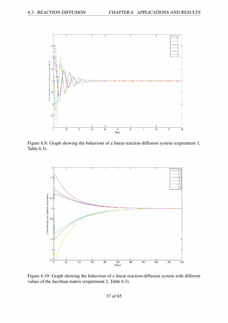
6.3. REACTION-DIFFUSION CHAPTER 6. APPLICATIONS AND RESULTS
Figure 6.9: Graph showing the behaviour of a linear reaction-diffusion system (experiment 1,Table 6.3).
Figure 6.10: Graph showing the behaviour of a linear reaction-diffusion system with differentvalues of the Jacobian matrix (experiment 2, Table 6.3).
37 of 65

6.3. REACTION-DIFFUSION CHAPTER 6. APPLICATIONS AND RESULTS
Figure 6.11: Graph showing that a linearised reaction-diffusion system is unstable if stabilityconditions are not satisfied (experiment 3 from Table 6.3).
Figure 6.12: Graph showing the same linear system as in experiment 1 but without diffusion(experiment 4, Table 6.3).
38 of 65

6.3. REACTION-DIFFUSION CHAPTER 6. APPLICATIONS AND RESULTS
Table 6.4: Experiments on how a linear system is affected from diffusion.
No. A No. of cells Diffusion coefficients (M) Initial state
1(
0.6171 0.8244−1.6432 −0.8824
)3
(0.025 0
0 0.05
)Random
2(
0.6171 0.8244−1.6432 −0.8824
)3
(2.5 00 5
)Random
3(
0.6834 0.4423−2.1634 −1.3875
)3
(0.025 0
0 0.05
)Random
4(
0.6834 0.4423−2.1634 −1.3875
)3
(40 00 80
)Random
Results do not prove or show regarding the way that diffusion affects the system. Tryingto perform the same tests by changing the diffusion coefficients only is shown in Table 6.4 andfigures 6.13, 6.14 opposed to 6.9 and 6.10 respectively.
Notice now that only two colours are visible in the graph 6.10. That means that morphogenconcentrations in cells are equal and thus, with high diffusion coefficients (40 and 80) all cellsrapidly become identical. This means that large diffusion coefficients must be avoided in orderto differentiate cells.
The general conclusion is that diffusion is very important in morphogenesis and has a highimpact on the behaviour of the system. Despite the fact that graphs show identical behaviour, itshould not be neglected that the purpose of the project is to generate software applications thatpresent how cells create structures. Cells must have properties that differentiate one-another.By setting a large diffusion coefficient value, cells may become quickly identical and the inter-nal chemical reactions will not lead into different results. The choice of diffusion coefficientsis therefore critical.
6.3.2 Non-linear modelsThe non-linear models discussed in Chapter 4 were used to the final software solutions. Themain purpose was to show how cells are organising and form structures out of a random chaoticstate. The results are shown in images that represent the structure of the system. Those imagesare snapshots of the system at time zero, middle and final point snapshots are arranged in atimeline.
Table 6.5 shows the parameters and the models that were used. Notice that diffusion coef-ficients and the number of cells affect the structure of the system.
As shown in Figures 6.15-6.20, a variety of different structures is obtained. The cells startwith a randomly initialised state, but they form shapes and patterns progressively in time.
6.3.3 Introducing mutationA physical system in the real world is never isolated. External factors or random events mightaffect the cells by changing their state. This phenomenon is called mutation and one of thereasons, for example, for producing cancerous masses in advanced biological organisms orcausing changes of characteristics (for instance, change in the eye colour). In some organisms,
39 of 65

6.3. REACTION-DIFFUSION CHAPTER 6. APPLICATIONS AND RESULTS
Figure 6.13: Graph showing how the behaviour of the linear system differantiates with largediffusion coefficients (experiment 2, Table 6.4 opposed to experiment 1, Figure 6.9).
Figure 6.14: Graph showing how the behaviour of the linear system differantiates with verylarge diffusion coefficients (experiment 4, Table 6.4 opposed to experiment 3, figure 6.10).
40 of 65

6.3. REACTION-DIFFUSION CHAPTER 6. APPLICATIONS AND RESULTS
Table 6.5: Experiments of non-linear models with various parameters.No. Model Parameters Diffusion Coefficients Number of Cells1 L-Systems None Du = 1.6,Dv = 6 64002 L-Systems None Du = 1.6,Dv = 6 225003 L-Systems None Du = 3.5, Dv = 16 64004 L-Systems None Du = 2, Dv = 5 64005 Gray Scott F = 40,k = 60 Du = 1, Dv = 16 225006 Gray Scott F = 30,k = 40 Du = 1, Dv = 16 22500
Figure 6.15: Initial, middle and final snapshots of the structure of the L-systems of experimentNo. 1, Table 6.5.
Figure 6.16: Initial, middle and final snapshots of the structure of the L-systems with morecells as shown in experiment 2, Table 6.5.
Figure 6.17: Initial, middle and final snapshots of the structure of the L-systems with differentdiffusion coefficients (experiment 3, Table 6.5).
41 of 65

6.3. REACTION-DIFFUSION CHAPTER 6. APPLICATIONS AND RESULTS
Figure 6.18: Initial, middle and final snapshots of the structure of the L-systems with differentdiffusion coefficients (experiment 4, Table 6.5).
Figure 6.19: Initial, middle and final snapshots of the structure of the Gray-Scott model withparameters shown in experiment No.5, Table 6.5.
Figure 6.20: Initial, middle and final snapshots of the structure of the Gray-Scott model withdifferent reaction rates (experiment No.5, Table 6.5).
42 of 65

6.3. REACTION-DIFFUSION CHAPTER 6. APPLICATIONS AND RESULTS
Table 6.6: Showing the effect of mutation on different probabilities.
No. Diffusion Coefficients Number of Cells Mutation Probability Number of mutated cells1 Du = 1.6,Dv = 6 3600 0.001 22 Du = 1.6,Dv = 6 3600 0.01 39
Figure 6.21: Initial state, final structure before mutation , and recovered structure after mutationwith mutation probability 0.001 (experiment 1, Table 6.6).
controlled mutations may have desirable effects. In agriculture, grafting takes place in plantsto make them produce better fruit [17]. Mutation occurs under different circumstances, butthe concept remains the same; the behaviour of a system is changed by altering some of itsproperties.
A study on altering the system randomly after its development is proposed. The processis that the system is left to evolve for a specific amount of time. Then, random perturbationschange some cells by altering their morphogen concentrations and the system is integratedagain. The purpose is to find at what mutation probabilities the structure of the system ischanged dramatically beyond recovery.
This can be done by observing the structures prior to and following mutation. Due tothe colour mapping, a single cell mutation may lead to the false conclusion that the structurechanged rapidly but this is not the case. What one should observe is whether the change insome cells can be absorbed by the system and if the system recovers to its previous structure.
The results show that a probability of cell mutation equal to 0.01 is sufficient to alter the
Figure 6.22: Initial state, final structure before and after mutation showing that with probability0.01 the structure changes (experiment 2, Table 6.6).
43 of 65

6.4. PRODUCING SOUND CHAPTER 6. APPLICATIONS AND RESULTS
Figure 6.23: Pattern produced by the Gizburg-Landau model.
final structure of a system.More ideas arise on how to experiment with mutation. One is to find the highest probability
at which a system can recover. As shown, a probability of 0.01 caused the structure of thesystem to change while the probability of 0.001 did not affect the system. What may be thethreshold that brings the system to its limit?
Another idea would be to simulate the method of grafting. In this method, a tissue is takenfrom a plant and is inserted into another one. That process may transform, for example, a partof a mandarin tree to become an orange tree. A similar approach can be used to visualise thisconcept. A way of accomplishing this could be to generate two structures. In practice, thestructures are matrices, in theory they are systems of cells. Then, take from the two structuresa portion (a column, a row, or a small square portion) of each and substitute them. How willeach structure be after integration? This is an interesting experiment that expands the results ofthis section.
6.4 Producing soundMathematical models of morphogenesis have oscillatory behaviour. Thus, they share a com-mon behaviour with sound. The sinusoidal waves of a mathematical reaction-diffusion modelcan be converted into frequency spectra and then sound may be produced by driving the spectravalues to the sound card.
A mathematical model that presents continuous waves is needed. The Gizburg-Landau wasused as was analysed and implemented by Aly-Khan Kassam [4] Figure 6.23 shows the patternthat this model generates.
There are various ways for extracting frequency spectra values from the waves that theGizburg-Landau model generates. The problem is the same with colour values: to find theright way for mapping the morphogen concentrations into frequency values. The method thatwas followed was to get the mean of the morphogen concentrations for each point in time. Theresult is shown in Figure 6.24.
6.5 Comparing schedulersThe scheduling solution described in Section 5.2.3 involved four schedulers. The randomscheduler, a priority scheduler, the Round Robin Scheduler and the project-related diffusion-scheduler. The results show a similar performance of the Round Robin and the Diffusion
44 of 65
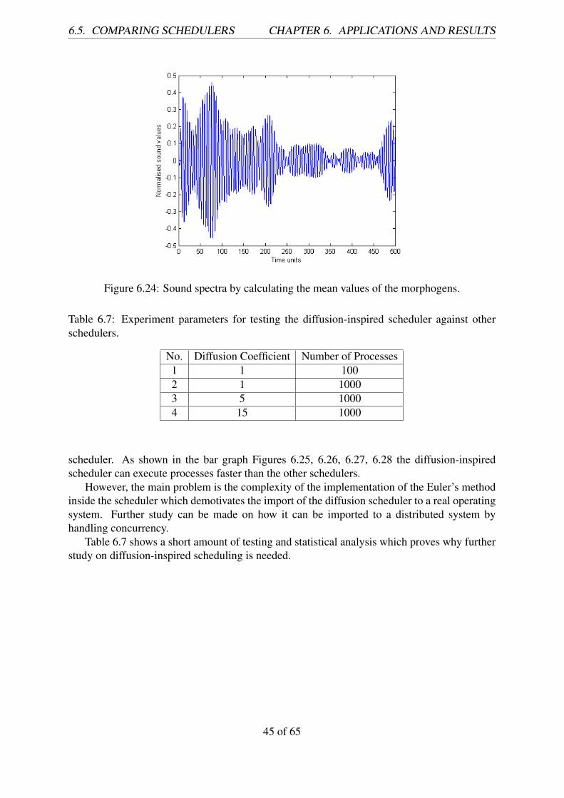
6.5. COMPARING SCHEDULERS CHAPTER 6. APPLICATIONS AND RESULTS
Figure 6.24: Sound spectra by calculating the mean values of the morphogens.
Table 6.7: Experiment parameters for testing the diffusion-inspired scheduler against otherschedulers.
No. Diffusion Coefficient Number of Processes1 1 1002 1 10003 5 10004 15 1000
scheduler. As shown in the bar graph Figures 6.25, 6.26, 6.27, 6.28 the diffusion-inspiredscheduler can execute processes faster than the other schedulers.
However, the main problem is the complexity of the implementation of the Euler’s methodinside the scheduler which demotivates the import of the diffusion scheduler to a real operatingsystem. Further study can be made on how it can be imported to a distributed system byhandling concurrency.
Table 6.7 shows a short amount of testing and statistical analysis which proves why furtherstudy on diffusion-inspired scheduling is needed.
45 of 65

6.5. COMPARING SCHEDULERS CHAPTER 6. APPLICATIONS AND RESULTS
Figure 6.25: Comparison of the scheduler implementations with 100 processes in the queue(experiment No. 1 of Table 6.7).
Figure 6.26: Comparison of the scheduler implementations with 1000 processes in the queue(experiment No. 2 of Table 6.7).
46 of 65

6.5. COMPARING SCHEDULERS CHAPTER 6. APPLICATIONS AND RESULTS
Figure 6.27: Comparison of the scheduler implementations with 1000 processes in the queueand a different diffusion coefficient (5) for the diffusion-inspired scheduler (experiment No. 3of Table 6.7).
Figure 6.28: Comparison of the scheduler implementations with 1000 processes in the queueand the diffusion coefficient of the diffusion-inspired scheduler being 15 (experiment No. 4 ofTable 6.7).
47 of 65

Chapter 7
Software development
The software development process involved implementing simulations for the mathematicalmodels described in Chapter 4, testing that involved a basic mathematical analysis of eachmodel and documentation of the work. The methodologies that were followed during theproject can be used as a reference for the reader in order to follow or improve such a methodfor future research or a related project. It can also be used as a method of understanding thecoding structure and then expanding the ideas that are introduced in this project.
7.1 Model simulationsThe main deliverable concerning model simulations is a Matlab application. The methodologyis discussed to help the reader in using the application and its source code. It might also beused as a guide for solving similar problems.
7.1.1 Code structureThe code has three main components:
• The main function that prompts the user to initialise certain parameters of the model, suchas the number of cells and the amount of time to be used in integrating the equations.
• A nested function in the body of the main function that calculates the equations of acertain model. Whether it can be uncoupled from the main function is debatable; it iseasier to share variables from the main function to the nested one.
• Global external functions that can be used by any application and can be easily im-ported by anyone who is interested in using them. Examples of such functions are theplayMovie and scaleColors.
Globally available functions are shown in appendixA.
7.1.2 TestingTesting mathematical models is challenging. In general, software testing is done by comparingthe output of a body of code with hard-coded data (that is, the expected output). For testing amathematical model, an analysis of that model needs to be done first, in order to identify what
48 of 65

7.2. PROCESS SCHEDULING CHAPTER 7. SOFTWARE DEVELOPMENT
behaviour is expected. The analysis can be automated with the use of the symbolic computa-tional capabilities of Matlab [11] or Mathematica [18].
Testing of function implementation that do not involve integration of a system of equationsis done in a traditional approach; the output results of a function for certain inputs are comparedto expected outputs for those input values. The scaleColors function is a crucial function tothe system, since it is a key part in mapping the morphogen concentrations to color interpretedvalues. It takes an array of morphogen concentrations and normalises their values to the rangeof [0,1] according to the maximum and minimum concentrations.
7.1.3 DocumentationDocumentation of the work is presented in HTML format. The purpose of documenting theMatlab functions is to provide a quick reference of the functions implemented, their argumentsand their interdependence. In order to automate the process of documentation a Bash scriptwas created that gets a set of Matlab files and creates HTML files that provide information ofthe functions in each file (see bash scripts C.2 and C.1).
7.2 Process schedulingThe deliverable is a framework written in Java that can be used for:
1. Creating Scheduler algorithms.
2. Implementing ODE solvers.
3. Defining mathematical models.
4. Running and retrieving statistical results for each scheduler.
An additional tool written in bash script and gnuplot script is provided for converting the sta-tistical information generated by the Java implementation into bar graphs. All scripts can befound in Appendix C.
7.2.1 MethodologyThe framework is meant to be used by anyone that wants to experiment with the idea of schedul-ing by solving differential equations. Thus, the use of software design patterns was essential inorder to make the code readable and easy to be expanded. Documentation was generated withproper commenting of the code and then the use of javadoc [21] and testing was done withgraph generation by using gnuplot scripts.
7.2.2 Code structureAll class files are included in a single package. The naming of the files is based on softwaredesign patterns. Testing was done by the use of bash scripts and the use of the test class”TestScheduler” for the schedulers. The graphs for analysing the effectiveness of each algo-rithms were generated with the program gnuplot and bash scripts to create data files for thegnuplot scripts.
49 of 65
7.3. SCRIPTS AND TOOLS CHAPTER 7. SOFTWARE DEVELOPMENT
Software design patterns
A fair amount of software design patterns were used in order to make the code more readableand easier to maintain. The patterns were used in reference of the ‘Gang of Four’ [13] andGRASP [5].
The Template pattern was used to protect variations among various ODE solvers, equa-tions/functions and schedulers. A default implementation is given by either an interface or anabstract class and every class-object that provides a specific implementation extends that inter-face or abstract class. This helps in extending the framework with more ode solvers, schedulersor mathematical models.
A Memento pattern is used for the process classes, allowing them to restore to their initialstate and be reused different schedulers. This helps in the statistical analysis, because sched-ulers must be compared to each other under the same circumstances. For instance, a processis created with random properties such as how many time cycles are needed to finish at whichpoints in time it blocks or crashes etc. All process properties are shown in Figure 5.4.
7.2.3 TestingTesting was done by producing graph plots and bar graphs in order to observe abnormalitiesin the parameters of the processes or schedulers. Abnormalities were expected by the useof wrong time step in the Euler’s method implementation or bugs in general that restrictedthe program to run according to its requirements. The graphs and plots were generated withgnuplot with a middle layer script written in bash. The role of the script was to convert the dataof the scheduler statistics into gnuplot data format.
7.3 Scripts and toolsA set of scripts were implemented in order to automate the process of testing, documentationand statistical analysis of the scheduling solutions. All scripts were written in Bash on a Linuxbased operating system. In addition, gnuplot was used in order to import data and generategraphs to visualise the statistical results. The decision for implementing separated scripts toautomate the tasks described was proved to have a significant positive impact during the projectdevelopment. Each script and its role is shown in Table 7.1.
50 of 65

7.3. SCRIPTS AND TOOLS CHAPTER 7. SOFTWARE DEVELOPMENT
File-name Language Description Source-codematdoc Bash Reads a matlab file that contains and creates a representative
HTML file that contains the functions defined in the matlabfile. Each function is given a description according to thecomments it has before its definition.
C.1
matdoc pages Bash Gets all HTML files and outputs an HTML body containinga list of links for those files. If its output is piped to a filecalled index, the whole documentation is ready to be read.
C.2
run-test Bash Executes the TestScheduler class of the process schedulingsolution with a given argument that represents the numberof processes existing initially in the queue and then, con-verts the output data into data that can be read by gnuplotscript.
C.4
run-tests Bash Gets 3 arguments: number of processes to start, numberof processes to finish and the step to reach that number ofprocesses. Then it calls run-tests and gets the generated datato plot them using the gnuplot script totalTime.p
C.5
totalTime.p gnuplot Reads a data file and generates the bar plots to visualise theresults as shown in paragraph 6.5.
C.3
Table 7.1: Description of the implemented scripts that automate documentation and testing.
51 of 65

Chapter 8
Conclusion
The project generated animations and movies that visualise how cells can form complex struc-tures. This was done with the use of two mathematical models, the Gray-Scott model and theL-Systems equations. A third model, the Gizburg-Landau was used to explore the possibilityof sound generation. The ordinary differential equations of those models, were integrated withthe ODE solvers of matlab and matrix operations. The results were shown as images by us-ing conversion algorithms to normalise chemical concentrations into ranges of colour values.Results were shown in the form of plotted graphs as well.
Further goals of the project were to exploit the idea of morphogenesis to research otherconcepts. One was to generate sound instead of images. Experimentation with sound led to thedefinition of ideas and implementation of tools which may be used in the future to explore thepossibility of audio production by the use of models of morphogenesis. The graph results ofthe project in terms of audio production present similarities to the sound waves. Thus, furtheranalysis and exploration of the concept is encouraged.
Next, the project studied how mutations affect the state of a system. The experiments takea finished structure of a system and alter the morphogen concentrations of some cells with agiven probability. Then, the system is integrated again. It has been shown that with a very lowprobability (0.001) that affects only a tiny amount of cells, the system recovers the structure.On the other hand, a probability of 0.01 is able to alter the structure of a system significantly.
The latter experiment arises further questions or ideas on how to use mutation to studymorphogenesis. What will happen if the mutation is done according to the values of a differentsystem, in the same way that grafting is done for plants? What would be the outcome if themutation changes the diffusion coefficients as well? Is there a way to recover the system toregain its pre-mutant structure?
The last goal was to find a way to apply the concepts of morphogenesis in a computerscience problem. The ‘diffusion-inspired algorithm’ was to create a process scheduler thatuses diffusion to give each process different time slices on which processes are allowed tobe executed. Although the algorithm has a high computational complexity it seems to be moreeffective than a random scheduler or a priority scheduler. The difference between the diffusion-inspired scheduler and the Round Robin is very small. For some parameters the diffusion-inspired scheduler even seems to have less inactivity and less total time than the Round Robin.
There are a lot of parameters in the scheduling problem that have not been addressed. Thediffusion-inspired scheduler was not compared to itself with different parameters. In addition,schedulers may be tested with processes that have high or low rates in requesting input/outputtime. Thus, exploring on which environments each scheduler is best, or which parameters make
52 of 65

CHAPTER 8. CONCLUSION
the diffusion-inspired scheduler better in different environments is suggested. The softwareframework that was developed provides easy to maintain and expand code motivating furtherexperiments.
The project combined a mixture of biology, chemistry, mathematics, engineering and com-puter science. Time limited further investigation of more conepts and ideas. The conclusion ofall this work, is that morphogenesis is not just a mathematical model that generates patterns.It is a framework enabling the testing of physical systems, which has the potential to give newideas and applications for researching or experimenting with concepts that reflect in the reallife world.
53 of 65

Bibliography
[1] A. M. Turing, “The chemical basis of morphogenesis,” Philosophical Transactions of theRoyal Society of London. Series B, Biological Sciences, vol. 237, no. 1, 1952.
[2] M. R. Garvie, P. K. Maini, and C. Trenchea, “A Methodology for Parameter Identificationin Turing Systems,”
[3] B. M. Heineike, “Modeling morphogenesis with reaction-diffusion equations usinggalerkin spectral methods,” tech. rep., DTIC Document, 2002.
[4] A.-K. Kassam, “Solving reaction-diffusion equations 10 times faster,” 2003.
[5] C. Larman, Applying UML and Patterns: An Introduction to Object-Oriented Analysisand Design and Iterative Development. Prentice Hall, 3 ed., Oct. 2004.
[6] J. S. McGough and K. Riley, “Pattern formation in the GrayScott model,” vol. 5, no. 1,p. 105121, 2004.
[7] C. G. Jennings, “Turing’s reaction-diffusion model of morphogenesis,” January 2011.
[8] L. Perko, Differential Equations and Dynamical Systems. New York: Springer, 2001.
[9] J. K. Aggarwal, Notes on Nonlinear Systems. Van Nostrand Reinhold, Jan. 1972.
[10] F. Diacu, Differential Equations: Order and Chaos: An Introduction to Differential Equa-tions. W. H. Freeman, Oct. 2000.
[11] MATLAB, version 7.10.0 (R2010a). Natick, Massachusetts: The MathWorks Inc., 2010.
[12] T. Williams and C. Kelley, “Gnuplot.”
[13] E. Gamma, R. Helm, R. Johnson, and J. Vlissides, Design Patterns CD: Elements ofReusable Object-Oriented Software. Addison Wesley, 1 ed., May 1998.
[14] O. Koch, P. Kofler, and E. B. Weinmller, “The implicit euler method for the numeri-cal solution of singular initial value problems,” Applied numerical mathematics, vol. 34,no. 2-3, p. 231252, 2000.
[15] A. S. Tanenbaum, Modern Operating Systems. Pearson, 3 ed., Dec. 2007.
[16] S. Childress, “Case sudy 2: Turings model of chemical morphogenesis,” 2005.
[17] A. Nelson, Principles of Agricultural Botany. Lightning Source Incorporated, Mar. 2007.
54 of 65

BIBLIOGRAPHY BIBLIOGRAPHY
[18] Mathematica, version 8.0.4. Wolfram, 2011.
[19] J. P. La Salle, Lecture notes on stability and control. Center for Dynamical Systems;Division of Applied Mathematics, Brown University, 1966.
[20] S. Lynch, S. Lynch, and Birkhauser, Dynamical Systems with Applications using MAT-LAB. Birkhuser, 2004 ed., June 2004.
[21] javadoc, version 5.0. Oracle.
55 of 65

Appendices
56 of 65

Appendix A
Matlab programs
A.1 Template reaction diffusion model.m
%%C a l l t h i s f u n c t i o n t o run a r e a c t i o n−d i f f u s i o n model from%%L−S y s t e m s and have v i s u a l v iew o f how t h e c e l l s g e t o r g a n i s e df u n c t i o n nlm = r e a c t i o n d i f f u s i o n m o d e l ( )
Du = 1 . 6 ; %d i f f u s i o n c o e f f i c i e n t 1Dv=6; %d i f f u s i o n c o e f f i c i e n t 2NumberOfCel ls= input ( ’ Number o f c e l l s : ’ ) ;s i d e = s q r t ( NumberOfCel ls ) ;h = 0 . 0 1 ;
systemU= i m a g e T o P a t t e r n ( random ( ’ norm ’ , 0 , 1 , s i d e , s i d e )∗12 + random ( ’ u n i f ’ , 0 , 1 , s i d e , s i d e )∗2 , 5 ) ;systemV= i m a g e T o P a t t e r n ( random ( ’ norm ’ , 0 , 1 , s i d e , s i d e )∗12 + random ( ’ u n i f ’ , 0 , 1 , s i d e , s i d e )∗2 , 5 ) ;s i d e = s i z e ( systemU , 1 ) ;NumberOfCel ls = s i d e ∗ s i d e ;sys tem =[ Two2oneD ( systemU ) ; Two2oneD ( systemV ) ] ;t L i m i t = input ( ’ Time l e n g t h : ’ ) ;t s p a n = [0 t L i m i t ] ;o p t i o n s = o d e s e t ( ’ NonNegat ive ’ , ( 1 : s i d e ∗ s i d e ) ) ;
[ t , uv ] = ode45 (@im, t s p a n , abs ( sys tem ) , o p t i o n s ) ;p l o t ( t , uv ) ;
input ( ’ P r e s s e n t e r t o p r o c e e d t o movie ’ ) ;f i g 1 = f i g u r e ( 1 ) ;w i n s i z e = g e t ( f i g 1 , ’ P o s i t i o n ’ ) ;w i n s i z e ( 1 : 2 ) = [0 0 ] ;numframes= l e n g t h ( t ) ;A=moviein ( numframes , f i g 1 , w i n s i z e ) ;s e t ( f i g 1 , ’ N e x t P l o t ’ , ’ r e p l a c e c h i l d r e n ’ ) ;
f o r i =1 : numframesimshow ( i m r e s i z e ( c e l l s T o S u r f ( i , uv , s i d e ) , [ 3 0 0 , 3 0 0 ] ) ) ;
A ( : , i )= getframe ( f i g 1 , w i n s i z e ) ;endmovie ( f i g 1 , A, 1 , 5 , w i n s i z e ) ;
movie2av i (A, ’ movie . a v i ’ ) ;
%%C a l l t h i s i n s i d e an ode s o l v e r t o s o l v e an L−S y s t e m s e q u a t i o n w i t h d i f f u s i o n i n a t o r u sf u n c t i o n i n t e g r a t e m o d e l = im ( t s p a n , c e l l s )
U= c e l l s ( 1 : l e n g t h ( c e l l s ) / 2 ) ;V= c e l l s ( l e n g t h ( c e l l s ) / 2 + 1 : end ) ;
57 of 65

A.2. TEMPLATE PLAYMOVIE.M APPENDIX A. MATLAB PROGRAMS
f o r c =1: l e n g t h (U ) ;
a d j = g e t a d j a c e n t s ( c , s i d e ) ;d i u ( c )=Du∗ (U( a d j ( 1 ) ) + U( a d j ( 2 ) ) + U( a d j ( 3 ) ) + U( a d j ( 4 ) ) − 4∗U( c ) ) ; %d i f f u s i o n Ud i v ( c )=Dv∗ (V( a d j ( 1 ) ) + V( a d j ( 2 ) ) + V( a d j ( 3 ) ) + V( a d j ( 4 ) ) − 4∗V( c ) ) ; %d i f f u s i o n VReu ( c )=U( c )∗V( c ) − U( c ) − 1 2 ;Rev ( c )=16−U( c )∗V( c ) ;dU ( c )= Reu ( c )+ d i u ( c ) ;dV ( c )= Rev ( c ) + d i v ( c ) ;
end
i n t e g r a t e m o d e l = [ dU ’ ; dV ’ ] ;end
end
A.2 Template playMovie.m
%%g e t s an Array o f s i z e s i z e ( t i m e ) c o n t a i n i n g f ram es nxm andf u n c t i o n playMovie ( gl , t ime )
input ( ’ P r e s s e n t e r t o p r o c e e d t o movie ’ ) ;f i g 1 = f i g u r e ( 1 ) ;w i n s i z e = g e t ( f i g 1 , ’ P o s i t i o n ’ ) ;w i n s i z e ( 1 : 2 ) = [0 0 ] ;numframes= l e n g t h ( t ime ) ;A=moviein ( numframes , f i g 1 , w i n s i z e ) ;s e t ( f i g 1 , ’ N e x t P l o t ’ , ’ r e p l a c e c h i l d r e n ’ ) ;s i z e ( g l ( 1 ) )f o r j =1 : numframes
imshow ( g l ( : , : , j ) ) ;
A ( : , j )= getframe ( f i g 1 , w i n s i z e ) ;endmovie ( f i g 1 , A, 1 , 5 , w i n s i z e ) ;
movie2av i (A, ’ movie . a v i ’ ) ;%g l=r e a l ( i f f t n ( v ) ) ;
end
A.3 Template initialiseA.m
f u n c t i o n i n i t i a l i s e A = e q p o i n t ( )%c u r r e n t l y works w i t h 2 c h e m i c a l sa11=rand ( ) ;a22=−a11−rand ( ) ;a12=rand ( ) ;a21 =( a11∗ a22 ) / a12 − rand ( ) ;i n i t i a l i s e A =[ a11 a12 ; a21 a22 ] ;
58 of 65

Appendix B
Java programs
B.1 AbstractFunction.java
/∗ ∗∗∗ P r o v i d e s an i m p l e m e n t a t i o n o f a f u n c t i o n so i t can be∗ used i n v a r i o u s ode ’ s . I n s t e a d o f d e v e l o p i n g a s y m b o l i c∗ s o l v e r t h i s i s t h e e a s i e s t way t o p r o t e c t v a r i a t i o n s f o r each f u n c t i o n .∗ @author n i c o l a v 0∗∗ /
p u b l i c a b s t r a c t c l a s s A b s t r a c t F u n c t i o n{
p r o t e c t e d double r e s u l t = 0 ;
/∗ ∗∗∗ @param elems∗ @param params∗ @return r e s u l t∗ D e f i n e s t h e a c t u a l f u n c t i o n and c a l c u l a t e s t h e r e s u l t s∗ /
p r o t e c t e d a b s t r a c t double c a l c u l a t e ( i n t elems , double . . . params ) ;
/∗ ∗∗∗ @param elems∗ @param params∗ @return a new c a l c u l a t e d r e s u l t∗ C a l l t h i s method t o run a c a l c u l a t i o n o f t h e f u n c t i o n and g e t a new r e s u l t∗ /
p u b l i c double g e t R e s u l t ( i n t elems , double . . . params ){
r e s u l t = c a l c u l a t e ( elems , params ) ;re turn r e s u l t ;
}
/∗ ∗∗∗ @param elems∗ @param params∗ @return a new c a l c u l a t e d r e s u l t∗ Over load t o e n s u r e t h a t t h e use o f Double i n s t e a d o f d oub l e does∗ n o t a f f e c t t h e f u n c t i o n a l i t y∗ /
p u b l i c double g e t R e s u l t ( i n t elems , Double . . . params ){
i n t i = 0 ;double [ ] v a l u e s = new double [ params . l e n g t h ] ;f o r ( Double d : params ){
59 of 65

B.2. ODE.JAVA APPENDIX B. JAVA PROGRAMS
v a l u e s [ i ++] = d . doub leVa lue ( ) ;}r e s u l t = c a l c u l a t e ( elems , v a l u e s ) ;re turn r e s u l t ;
}
/∗ ∗∗ g e t t h e l a s t c a l c u l a t e d r e s u l t , u s e f u l t o check t h e p r e v i o u s∗ v a l u e i f t h e r e i s one b e f o r e r u n n i n g a n o t h e r c a l c u l a t i o n∗ @return p r e v i o u s r e s u l t∗ /
p u b l i c double g e t R e s u l t ( ){
re turn r e s u l t ;}
}
B.2 ODE.java
/∗ ∗∗ i n t e r f a c e f o r i m p l e m e n t i n g ODE s o l v e r s∗ @author n i c o l a v 0∗∗ /
p u b l i c i n t e r f a c e ODE{
void i n t e g r a t e ( i n t s t e p s , double [ ] i n i t i a l C o n d i t i o n s , double h ) ;
double [ ] [ ] s o l v e ( i n t s t e p s , double [ ] i n i t i a l C o n d i t i o n s , double h ) ;
double [ ] g e t R e s u l t ( i n t t ime ) ;
double [ ] [ ] g e t R e s u l t s ( ) ;
p u b l i c S t r i n g t o S t r i n g ( ) ;
}
B.3 AbstractODE.java
/∗ ∗∗ c l a s s t h a t p r o v i d e s a framework f o r v a r i o u s ODE s o l v e r s∗ t o be imp lemen ted .∗ @author n i c o l a v 0∗∗ /
p u b l i c a b s t r a c t c l a s s AbstractODE implements ODE{
p r o t e c t e d double [ ] [ ] r e s u l t ;A b s t r a c t F u n c t i o n f ;/∗ ∗∗ each s o l v e r r e q u i r e s a f u n c t i o n t h a t w i l l i n t e g r a t e∗ @param f∗ /
p u b l i c AbstractODE ( A b s t r a c t F u n c t i o n f ){
t h i s . f = f ;r e s u l t = n u l l ;
}
/∗ ∗∗ @param s t e p s∗ @param i n i t i a l C o n d i t i o n s
60 of 65

B.4. SCHEDULER.JAVA APPENDIX B. JAVA PROGRAMS
∗ @param h∗ C a l l t h i s t o i n t e g r a t e your e q u a t i o n . I t needs t h e i m p l e m e n t a t i o n o f s o l v e ( )∗ /
p u b l i c vo id i n t e g r a t e ( i n t s t e p s , double [ ] i n i t i a l C o n d i t i o n s , double h ){
r e s u l t = new double [ s t e p s + 1 ] [ i n i t i a l C o n d i t i o n s . l e n g t h ] ;r e s u l t = s o l v e ( s t e p s , i n i t i a l C o n d i t i o n s , h ) ;
}
/∗ ∗∗ imp lemen t t h i s so you can c a l l i n t e g r a t e∗ /
p u b l i c a b s t r a c t double [ ] [ ] s o l v e ( i n t s t e p s , double [ ] i n i t i a l C o n d i t i o n s , double h ) ;
p u b l i c double [ ] g e t R e s u l t ( i n t t ime ){
re turn r e s u l t [ t ime ] ;}
/∗ ∗∗ g e t t h e r e s u l t s i n an a r r a y o f d oub l e t i m e x r e s u l t s∗ /
p u b l i c double [ ] [ ] g e t R e s u l t s ( ){
re turn r e s u l t ;}
/∗ ∗∗ Human r e a d a b l e r e p r e s e n t a t i o n o f t h e s o l u t i o n∗ /
p u b l i c S t r i n g t o S t r i n g ( ){
S t r i n g o u t p u t = ” R e s u l t \n========\n ” ;f o r ( i n t i =0 ; i < r e s u l t . l e n g t h ; i ++){
o u t p u t +=” S tep ” + i + ” : ” ;f o r ( i n t j =0 ; j < r e s u l t [ i ] . l e n g t h ; j ++)
o u t p u t += r e s u l t [ i ] [ j ] + ” ” ;o u t p u t +=”\n ” ;
}re turn o u t p u t ;
}}
B.4 Scheduler.java
import j a v a . u t i l . A r r a y L i s t ;import j a v a . u t i l . A r r ay s ;import j a v a . u t i l . L i s t ;/∗ ∗∗ p r o v i d e s a framework f o r i m p l e m e n t i n g v a r i o u s s c h e d u l e r s .∗ @author n i c o l a v 0∗∗ /
p u b l i c a b s t r a c t c l a s s S c h e d u l e r {
p r o t e c t e d s t a t i c double s l i c e S i z e = 0 . 0 0 1 ;
p r o t e c t e d L i s t <P r o c e s s> p r o c e s s e s ;p u b l i c S c h e d u l e r ( ){
p r o c e s s e s = new A r r a y L i s t <P r o c e s s > ( ) ;}
p u b l i c vo id a d d P r o c e s s ( P r o c e s s p ){
p r o c e s s e s . add ( p ) ;}
p u b l i c P r o c e s s g e t P r o c e s s ( i n t i n d e x )
61 of 65
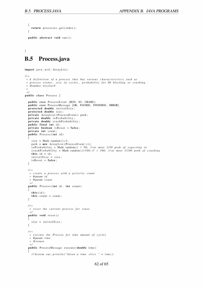
B.5. PROCESS.JAVA APPENDIX B. JAVA PROGRAMS
{re turn p r o c e s s e s . g e t ( i n d e x ) ;
}
p u b l i c a b s t r a c t vo id run ( ) ;
}
B.5 Process.java
import j a v a . u t i l . A r r a y L i s t ;
/∗ ∗∗ A d e f i n i t i o n o f a p r o c e s s t h a t has v a r i o u s c h a r a c t e r i s t i c s such as∗ p r o c e s s e v e n t s , s i z e i n c y c l e s , p r o b a b i l i t y f o r IO b l o c k i n g or c r a s h i n g .∗ @author n i c o l a v 0∗∗ /
p u b l i c c l a s s P r o c e s s {
p u b l i c enum P r o c e s s E v e n t {RUN, IO , CRASH} ;p u b l i c enum Proces sMessage {OK, PAUSED, FINISHED , ERROR}p r o t e c t e d double i n i t i a l S i z e ;p r o t e c t e d double s i z e ;p r i v a t e A r r a y L i s t <P r o c e s s E v e n t> p a t h ;p r i v a t e double i o P r o b a b i l i t y ;p r i v a t e double c r a s h P r o b a b i l i t y ;p u b l i c f i n a l i n t i d ;p r i v a t e boolean i s R e s e t = f a l s e ;p r i v a t e i n t c o u n t ;p u b l i c P r o c e s s ( i n t i d ){
s i z e = Math . random ( ) ∗ 3 ;p a t h = new A r r a y L i s t <P r o c e s s E v e n t > ( ) ;i o P r o b a b i l i t y = Math . random ( ) / 5 0 ; / / a t most 1 /50 prob o f e x p e c t i n g i oc r a s h P r o b a b i l i t y = Math . random ( ) / 1 0 0 ; / / / 100; / / a t most 1 /100 prob o f c r a s h i n gt h i s . i d = i d ;i n i t i a l S i z e = s i z e ;i s R e s e t = f a l s e ;
}
/∗ ∗∗ c r e a t e a p r o c e s s w i t h a p r i o r i t y c o u n t∗ @param i d∗ @param c o u n t∗ /
p u b l i c P r o c e s s ( i n t id , i n t c o u n t ){
t h i s ( i d ) ;t h i s . c o u n t = c o u n t ;
}
/∗ ∗∗ r e s e t t h e c u r r e n t p r o c e s s f o r r e u s e∗ /
p u b l i c vo id r e s e t ( ){
s i z e = i n i t i a l S i z e ;}
/∗ ∗∗ e x e c u t e t h e P r o c e s s f o r t i m e amount o f c y c l e s∗ @param t i m e∗ @return∗ /
p u b l i c Proces sMessage e x e c u t e ( double t ime ){
/ / Sys tem . o u t . p r i n t l n (” Given a t i m e s l i c e ” + t i m e ) ;
62 of 65

B.5. PROCESS.JAVA APPENDIX B. JAVA PROGRAMS
i n t t S t e p = 0 ;f o r ( double t =0 ; t <= t ime ; t += S c h e d u l e r . s l i c e S i z e ){
i f ( i s R e s e t ){
sw i t ch ( p a t h . g e t ( t S t e p ++) ){case IO :
p a t h . add ( P r o c e s s E v e n t . IO ) ;s i z e −=t ;re turn Proces sMessage . PAUSED;
case CRASH:re turn Proces sMessage .ERROR;
}
i f ( s i z e − t <= Math . exp (−10)){
re turn Proces sMessage . FINISHED ;}
}double c o n d i t i o n = Math . random ( ) ;i f ( c o n d i t i o n < i o P r o b a b i l i t y ){
p a t h . add ( P r o c e s s E v e n t . IO ) ;s i z e −=t ;
re turn Proces sMessage . PAUSED;}i f ( c o n d i t i o n < c r a s h P r o b a b i l i t y ){
p a t h . add ( P r o c e s s E v e n t .CRASH ) ;re turn Proces sMessage .ERROR;
}i f ( s i z e − t <= S c h e d u l e r . s l i c e S i z e ∗ 0 . 1 ){
re turn Proces sMessage . FINISHED ;}
}
s i z e −= t ime ;re turn Proces sMessage .OK;
}
/∗ ∗∗ g e t t h e p r i o r i t y o f t h i s p r o c e s s∗ @return∗ /
p u b l i c i n t g e t C ou n t ( ) {
re turn c o u n t ;}
}
63 of 65

Appendix C
Bash scripts and gnuplot scripts
C.1 matdoc# ! / b i n / bash#%% are d e s c r i p t i o n comments# main f u n c t i o n# %%# n e s t e d f u n c t i o n s
h=1IFS=$ ’\ n ’echo ”<html>”f o r l i n e i n ‘ e g r e p −w ” ∗%%.∗| ∗ f u n c t i o n .∗+ ” $1 ‘ ; do
comm= ‘ echo $ l i n e | g rep ”%%” ‘i f [ −n ”$comm” ] ; then
n e x t d e s c r i p t i o n = ‘ echo $comm | t r −d ’% ’ ‘;e l s e
i f [ ” $h ” −eq ” 1 ” ] ; then
echo ”<h$h>$ l i n e </h$h>”echo ”<p>$ n e x t d e s c r i p t i o n </p>”echo ”<ul><h2><b>Nes ted F u n c t i o n s </b></h2>”h =3;
e l s eecho ”< l i >”echo ”<h$h>$ l i n e </h$h>”echo ”<p>$ n e x t d e s c r i p t i o n </p>”echo ”</ l i >”
f i
f idoneecho ”</ u l>”echo ”</ html>”
C.2 matdoc pages
# ! / b i n / bashcd $1 ;c u r r d i r = ‘pwd ‘echo ”<html>”f o r f i l e i n ∗ . h tml ; do
echo ”<a h r e f =\” $ c u r r d i r / $ f i l e \”>$ f i l e </a><br>”doneecho ”</ html>”
C.3 totalTime.p
64 of 65

C.4. RUN-TEST APPENDIX C. BASH SCRIPTS AND GNUPLOT SCRIPTS
s e t t i t l e w i n d o w t i t l es e t s t y l e d a t a h i s t o g r a ms e t s t y l e h i s t o g r a m c l u s t e r gap 1
s e t s t y l e f i l l s o l i d b o r d e r rgb ” b l a c k ”s e t a u t o xs e t y ra ng e [ 0 : ∗ ]s e t y l a b e l ’ Time u n i t s ’p l o t ’ t i m e s d a t a . da t ’ u s i n g 2 : x t i c ( 1 ) t i t l e co l , \
’ ’ u s i n g 3 : x t i c ( 1 ) t i t l e co l , \’ ’ u s i n g 4 : x t i c ( 1 ) t i t l e co l , \’ ’ u s i n g 5 : x t i c ( 1 ) t i t l e c o l
C.4 run-test# ! / b i n / bash
# s e t g n u p l o t da ta f o r t o t a l t i m et o t a l T i m e s = ‘ j a v a T e s t S c h e d u l e r $1 | c a t > r e s u l t . log ‘t o t a l T i m e s = ‘ c a t r e s u l t . l o g | g rep ” T o t a l t ime : ” | c u t −d ’ : ’ −f 2 | t r −d ’ ’ ‘a v e r a g e s = ‘ c a t r e s u l t . l o g | g rep ” Average : ” | c u t −d ’ : ’ −f 2 | t r −d ’ ’ ‘a v g l i n e 1 = ‘ echo $ a v e r a g e s | c u t −d ’ ’ −f 1 , 3 , 5 , 7 ‘a v g l i n e 2 = ‘ echo $ a v e r a g e s | c u t −d ’ ’ −f 2 , 4 , 6 , 8 ‘t o t a l t i m e = ‘ echo $ t o t a l T i m e s | c u t −f 1−4‘{echo ” Time mesure ” ‘ c a t a l g o r i t h m s ‘echo ” i n a c t i v i t y $ a v g l i n e 1 ”echo ” l i f e c y c l e $ a v g l i n e 2 ”echo ” t o t a l $ t o t a l t i m e ”} | c a t > t i m e s d a t a . d a t# g n u p l o t −p t o t a l T i m e . p
C.5 run-tests# ! / b i n / bashf o r ( ( i =$1 ; i <=$2 ; i +=$3 ) ) ; do
. / run−t e s t $ ignuId = ‘ pgrep g n u p l o t ‘i f [ −n ” $gnuId ” ] ; then
k i l l $gnuIdf i
g n u p l o t −geomet ry 1600 x900 −d i s p l a y : 0 . 0 −e ” w i n d o w t i t l e = ’ P r o c e s s e s : $ i ’ ” −p t o t a l T i m e . ps l e e p 2
done
65 of 65