Computer-Aided Design 108 (2019) 30–41

Contents lists available at ScienceDirect

Computer-Aided Design

journal homepage: www.elsevier.com/locate/cad

Algebraic 3D graphic statics: Reciprocal constructionsMárton Hablicsek a,b, Masoud Akbarzadeh a,*, Yi Guo a

a Polyhedral Structures Laboratory, School of Design, University of Pennsylvania, Philadelphia, USAb Department of Mathematics, Centre of Symmetry and Deformation, University of Copenhagen, Denmark

a r t i c l e i n f o

Article history:Received 29 May 2018Accepted 15 August 2018

Keywords:Algebraic three-dimensional graphicstatics

Polyhedral reciprocal diagramsGeometric degrees of freedomStatic degrees of indeterminaciesTension and compression combinedpolyhedra

Constraint manipulation of polyhedraldiagrams

a b s t r a c t

The recently developed 3D graphic statics (3DGS) lacks a rigorous mathematical definition relatingthe geometrical and topological properties of the reciprocal polyhedral diagrams as well as a precisemethod for the geometric construction of these diagrams. This paper provides a fundamental algebraicformulation for 3DGS by developing equilibrium equations around the edges of the primal diagram andsatisfying the equations by the closeness of the polygons constructed by the edges of the correspondingfaces in the dual/reciprocal diagram. The research provides multiple numerical methods for solving theequilibriumequations and explains the advantage of using each technique. The approach of this paper canbe used for compression-and-tension combined form-finding and analysis as it allows constructing boththe form and force diagrams based on the interpretation of the input diagram. Besides, the paper expandson the geometric/static degrees of (in)determinacies of the diagrams using the algebraic formulationand shows how these properties can be used for the constrained manipulation of the polyhedrons in aninteractive environment without breaking the reciprocity between the two.

© 2018 Elsevier Ltd. All rights reserved.

1. Introduction

In graphic statics, the geometry of the structure and its equi-librium are represented by the form and force diagrams where thelength of themembers, the location of the supports and the appliedloads are represented by the former, and the equilibrium and themagnitude of the forces are represented by the latter. These twodiagrams are reciprocal, i.e. topologically dual and geometricallydependent [1]. In fact, themethods of graphic statics are essentiallythe geometric construction of these two reciprocal diagrams forvarious geometries, loading cases, and boundary conditions.

1.1. Reciprocal diagrams and their constructions

In 2D graphic statics, as it was developed and practiced inthe late nineteenth century, the construction of the reciprocaldiagrams was a step-by-step geometric construction [2–5]. Thisprocedural approach is quite cumbersome and lengthy for thestructures with multitudes of members, and any design iterationrequires a new construction process. This slow workflow could bethe reason for the shift towards the development of the numericalmethods at the end of the nineteenth century.

Graphic statics in combination with computational methodsresult in innovative design tools allowing the exploration of the

* Corresponding author.E-mail addresses: mhablicsek@math.ku.dk (M. Hablicsek),

masouda@upenn.edu (M. Akbarzadeh).

realm of unique, sophisticated, yet efficient structural solutions.Using computational methods can significantly accelerate theconstruction of the reciprocal diagrams and exploit the explicitrelationship between the form of a structure and its geometricequilibrium of forces in an interactive environment [6,7].

The topological and geometrical relationships between the re-ciprocal diagrams of 2D graphics statics (2DGS) have recently beenformulated as algebraically-constrained equations whose numer-ical solutions allow the direct construction of the diagrams in aninteractive environment [8,9]. Besides, the algebraic formulationof the graphic statics is a rigorous approach providing an in-depthunderstanding of some essential properties such as the geomet-ric/static degrees of indeterminacies of both form and force dia-grams. These parameters can be used interactively to manipulatethe geometry of these diagrams without breaking the reciprocitybetween them.

1.2. Problem statement and objectives

3DGraphical statics is a recent development of graphic statics inthree dimensions based on a historical proposition by Rankine [10]andMaxwell [1] [11–15]. In 3DGS, the form and the force diagramsare polyhedral diagrams; the equilibrium of each node of the formwith its applied loads/members is represented by a closed forcepolyhedron whose faces are perpendicular to the loads/membersof the node. The area of each face of the force polyhedron repre-sents the magnitude of the force in the corresponding member ofthe node.

https://doi.org/10.1016/j.cad.2018.08.0030010-4485/© 2018 Elsevier Ltd. All rights reserved.

M. Hablicsek, M. Akbarzadeh and Y. Guo / Computer-Aided Design 108 (2019) 30–41 31

Similar to 2DGS, the geometric construction of the recipro-cal polyhedral diagrams is the most crucial step in using 3DGSmethods. [16] explained a step-by-step procedural approach toconstruct both form and force diagrams of 3DGS for a given bound-ary conditions and loading scenario with the similar drawbacksof the procedural 2DGS methods. Additionally, [17] suggested acomputational implementation based on iterative geometric con-struction to find reciprocal forms for a given group of closed,convex polyhedral cells. Although the proposed method is quiterobust in generating the reciprocal diagrams, the precise controlof the edge lengths of the members of the diagrams is quite chal-lenging.Moreover, themethod cannot construct the reciprocals forcomplex/self-intersecting polyhedrons representing the systemswith both tension and compression members. Besides, any ma-nipulation introduced by the user in the geometry of the form orforce diagram breaks the reciprocity and requires a new iterativecomputation. In another research, [18] suggested the projectionof the polyhedral system to the fourth dimension and projectingit back to the third dimension by using paraboloid of revolutionthatmight be relatively counter-intuitive for the userswith limitedexperience with geometric constructions in 3D space.

In fact, in all mentioned methods, there is a lack of a propermathematical/algebraic formulation for the reciprocal polyhedraldiagrams limiting the interactive implementation of 3DGS. Thus,the primary objective of this paper is to provide an algebraicformulation to relate the reciprocal diagrams and a comprehensiveapproach to construct and manipulate the reciprocal polyhedronsfor compression/tension-only systems as well as the systems withboth tension and compression forces.

1.3. Paper outlines and contributions

Section 2 of this paper explains the theoretical framework ofthe research in the following order: the essential properties ofthe form and force diagrams including the nodal, global, and self-stressed polyhedrons (Section 2.1); the topological properties aswell as the incidence matrices to describe the connectivity of thecomponents of the primal and the dual diagrams (Sections 2.2, 2.3);the algebraic constraints between two reciprocal diagrams and theprocess of developing the equilibrium equations to find the lengthsof the edges of the dual diagram (Section 2.4); and the solutionspace for the equilibrium equations and the methods to constructthe geometry of the dual (Sections 2.5, 2.6). The algebraic approachof this research can construct the reciprocal diagram for bothform and force diagrams as the primal input. Therefore, Section 2also explains the procedures for the primal to be considered asa form or force diagram in the approach (Sections 2.7, 2.8), andexpands on the geometric and static degrees of (in)determinaciesof the systems based on the properties of the equilibrium matrix(Section 2.9).

Section 3 explains the computational implementation of thealgebraic formulation of 3DGS and provides three different numer-icalmethods for solving the equilibriumequations. In Section 4, theform finding, analysis, and constrained polyhedral manipulationapplications of the presentedmethod are explained and finally thelimitations, and the future research directions for this research arelisted in Section 5.

1.4. Nomenclatures

Wedenote the algebra objects of this paper as follows;matricesare denoted by bold capital letters (e.g. A); vectors are denoted bylowercase, bold letters (e.g., v), except the user input vectorswhichare represented byGreek letters (e.g.,λ); the topological data of theprimal diagram are described by italic letters (e.g., f ); and the datacorresponding to the dual and reciprocal diagram are representedby italic letters with a † sign (e.g., f †). Table 1 encompasses all thenotation used in the paper.

Table 1Nomenclature for the symbols used in this paper and their correspondingdescriptions.

Topology Description

Γ Primal diagramΓ † Dual, reciprocal diagramv # of vertices of Γe # of edges of Γf # of faces of Γc # of cells of Γv† # of vertices of Γ †

e† # of edges of Γ †

f † # of faces of Γ †

c† # of cells of Γ †

Matrices

Ce×v Edge–vertex connectivity matrix of ΓCe×f Edge–face connectivity matrix of ΓCf×c Face–cell connectivity matrix of ΓA Equilibrium matrixA+ Moore–Penrose inverse of AArref Reduced Row Echelon form of AArrefr×f Obtained by deleting all zero rows of Arref

Nx Diagonal matrix of the x-coords of n̂iNy Diagonal matrix of the y-coords of the n̂iNz Diagonal matrix of the z-coords of the n̂iL† Laplacian of Cf×c

Vectors

n̂i Unit normal vector of face fix x-coords of vy y-coords of vz z-coords of vu x-coord differences of vv y-coord differences of vw z-coord differences of vx† x-coords of v†

y† y-coords of v†

z† z-coords of v†

u† x-coord differences of v†

v† y-coord differences of v†

w† z-coord differences of v†q Solution of the equilibrium equations

Parameters

σ Parameter fixing the location of a vertex of Γ †

ξ Parameter for the Moore–Penrose inverse methodζ Parameter for RREF methodλ Parameter for the Linear programming method

Other

r Rank of Aψei Indicator of the type of internal forces of e†i

2. Theoretical framework

In this section, we briefly explain the properties of the recip-rocal polyhedral diagrams of the 3DGS and set a foundation todescribe the algebraic approach to construct these diagrams usinga simple example.

2.1. Form and force diagrams as groups of polyhedral cells

In the context of 3DGS, both form and force diagrams consist ofpolyhedral cells inwhich there is an external polyhedron includingall the external faces, and the rest of the cells are inside the externalpolyhedron. Each edge shares an identical vertex with its adjacentedges, and similarly, each face shares an identical edge with itsadjacent faces and finally, each cell shares an identical face withits adjacent cells.

Global and nodal force polyhedronsThe force diagram of 3DGS consists of closed polyhedral cells

that can be decomposed into the following: a global cell or global

32 M. Hablicsek, M. Akbarzadeh and Y. Guo / Computer-Aided Design 108 (2019) 30–41

Fig. 1. (a) A polyhedral structure with an applied load and reaction forces atthe support and (b) its corresponding force diagram consisting of 10 faces and 5polyhedral cells; (c) the global force polyhedron (GFP) with the direction of its facestoward inside the cell; and (d) the faces of GFP construct nodal force polyhedrons(NFP) whose directions are inherited from the faces of the GFP (three cells towardoutside (e.g. c1) and one toward inside (c0).

force polyhedron (GFP), and nodal cells or nodal force polyhedrons(NFP) [12,19]. A GFP represents the static equilibrium of exter-nally applied loads and reaction forces regardless of the geome-try/topology of the structure. Each NFP represents the equilibriumof forces coming together at that node in the form diagram. Similarto the form diagram, each cell in a group of cells can be chosenas the GFP; if GFP is the external polyhedron, the force diagramcan represent a compression/tension-only structural form. While,if GFP is any other cell except the external cell, the force diagramwill represent the equilibrium of a force configuration with bothtensile and compressive forces.

External loads and reaction forces of the formTo explain the external loads and reaction forces in the form

diagram, consider the example of a polyhedral joint with anexternally-applied force fk of Fig. 2a. This joint can be representedas a group of polyhedral cells in the context of 3DGS as shown inFig. 3a. Fig. 3a includes four open cells and no closed cell where theopen cells represent the applied loads, the reaction forces, and thelocation of the supports.

Generally, a group of polyhedral cells with no open cell mayrepresent a self-stressed system of forces with no externally-applied loads [1]. Replacing the dashed edges in the form diagramof Fig. 2b with additional members will turn the form into a self-stressed system [20]. Since in graphic statics we design the formdiagram for externally-applied loads and boundary conditions, sowe allow the form diagram to include open polyhedral cells [11].Subtracting a cell from a group of closed polyhedral cells resultsin both open and closed cells. We denote the subtracted cell theself-stress polyhedron (SSP) since the group of polyhedrons couldbe self-stressed otherwise.

In describing a form diagram, any cell, internal or external, canserve as the SSP. Subtracting the faces of SSP from the group ofpolyhedrons will leave the adjacent cells open and the rest of thecells closed. The edges connected to the vertices of the chosen SSPrepresent the vectors of the external loads and the reaction forces.The start point or the end point of the vectors can represent thelocation of the supports (up to translation). If the SSP is the external

Fig. 2. (a) A 3D structural joint with an applied force and internal forces in its mem-bers; (b) the form diagram/bar-node representation of the same joint in the contextof 3DGS; and (c) the force diagram/polyhedron representing the equilibrium of thesame node in 3DGS.

Fig. 3. (a) The primal diagram Γ and (b) its reciprocal diagram Γ † as called dualand their corresponding components.

polyhedron, all the internal edges connected to the vertices of theexternal polyhedron will represent the applied loads and reactionforces (Fig. 2b).

The direction of the cells in the form and force diagramsEach cell, in both form and force diagrams, has a direction either

towards inside or outside the cell that is defined by choosing thedirection for the SSP/GFP. The direction of the SSP/GFP is eithertowards inside or outside the cell. The faces of the cells adjacent tothe SSP/GFP will have the same direction as the faces of SSP/GFP.Every other cell in the group, if not adjacent to SSP/GFP, has anopposite direction of its adjacent cell.

For instance, consider the force diagram of Fig. 1a; the directionof the GFP is determined by the direction of the externally appliedloads and the reaction forces at the supports. The direction of theNFPs will be determined by the direction of GFP; each face of NFPthat is shared with the GFP will have the same orientation of theGFP face whereas, the face shared by another NFP will always havean opposite normal direction (Fig. 1b).

2.2. Topological and geometrical properties of the reciprocal polyhe-drons

We can use the example of Fig. 3 to explain the topologicalrelationship between reciprocal polyhedral diagrams. Let us callthe starting diagram the primal, Γ , and the reciprocal polyhedronthe dual, Γ † (Fig. 3a, b). The vertices, edges, faces, and cells of theprimal are denoted by v, e, f , and c respectively, and the ones of thedual are super-scripted with a dagger (†) symbol.

These two diagrams are topologically dual: i.e. the vertices v,edges e, faces f and cells c of the primal topologically map to thecells c†, faces f †, edges e† and vertices v†, respectively of the dualdiagram [11]. Therefore, the number of the dual elements in bothdiagrams is the same. For instance, the number of vertices v of the

M. Hablicsek, M. Akbarzadeh and Y. Guo / Computer-Aided Design 108 (2019) 30–41 33

Fig. 4. The primal diagram and the connectivity matrix given by its edges andvertices.

primal is equal to the number of cells c† in the dual, etc. Moreover,each edge e of the primal is perpendicular to its corresponding facef † in the dual.

2.3. Connectivity of the components

To formulate the algebraic relationship between the primal andthe dual diagrams, the relation between the components of eachdiagram should be described algebraically bymultiple connectivitymatrices for the vertices, edges, faces, and cells of the diagrams.

Edge–vertexLet us consider theprimal and thedual diagramsof Fig. 3a, b: the

primal diagram includes arbitrarily-indexed vertices and the edgespointing from a vertex with a smaller number to a vertex with abigger number (Fig. 4). For the primal diagram, the connectivitymatrix between the vertices and edges is a [e × v] matrix that isshown by Ce×v , described as

Cei,vj =

{+1 if vertex vj is the head of edge ei−1 if vertex vj is the tail of edge ei0 otherwise.

Since the edges and vertices of the primal map to faces andcells of the dual, matrix Ce×v is equal to Cf †×c† that represents theconnectivity of the faces and cells of the dual.

Edge–faceThe connectivity between edges and vertices, Ce×v , does not

describe the topology of the primal completely, and further con-nectivitymatrices are required to describe the topological relation-ships among other components of both primal and dual diagrams.Each face fi of the primal has a unit normal vector n̂i where thedirection of the normal may be chosen arbitrarily (Fig. 5). Thisdirection defines the orientation of the edges ei on that face usingthe right-hand rule.

Therefore, for each edge ei on the face fi there are twodirections:one given by matrix Ce×v and one defined by the direction of theunit normal of the face n̂i (Fig. 5). Thus, for the edges and their

Fig. 5. The connectivity of the faces and edges in the primal and its related matrix.

Fig. 6. The connectivity of faces and cells of the primal and its incidence matrix.

connected faces in the primal complex, the edge–face connectivitymatrix Ce×f is a [e × f ] matrix defined as

Cei,fj =

{+1 if edge ei is an edge of face fj−1 if opposite of edge ei is an edge of face fj0 otherwise.

Note that matrix Ce×f can also describe the connectivity be-tween the faces f † and edges e† of the dual complex and thus equalsmatrix Cf †×e† .

Face–cellTo complete the topological definition of the primal complex,

the connectivity between the faces and cells of the primal shouldbe described by an incidence matrix Cf×c . The direction of eachface fi in the primal was chosen arbitrarily. However, the directionof the cells is predefined as discussed in Section 2.1. We check

34 M. Hablicsek, M. Akbarzadeh and Y. Guo / Computer-Aided Design 108 (2019) 30–41

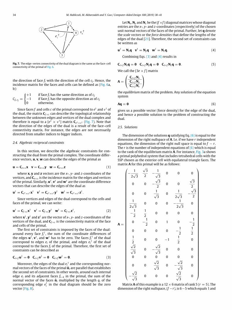
Fig. 7. The edge–vertex connectivity of the dual diagram is the same as the face–cellconnectivity of the primal of Fig. 6.

the direction of face fi with the direction of the cell cj. Hence, theincidence matrix for the faces and cells can be defined as (Fig. 6a,b):

Cfi,cj =

{+1 if face fi has the same direction as of cj−1 if face fi has the opposite direction as of cj0 otherwise.

Since faces f and cells c of the primal correspond to e† and v† ofthe dual, the matrix Cf×c can describe the topological relationshipbetween the unknown edges and vertices of the dual complex andtherefore is equal to a [e† × v†

] matrix Ce†×v† (Fig. 7). Note thatthe direction of the edges of the dual is a result of the face–cellconnectivity matrix. For instance, the edges are not necessarilydirected from smaller indices to bigger indices.

2.4. Algebraic reciprocal constraints

In this section, we describe the algebraic constraints for con-structing the dual from the primal complex. The coordinate differ-ence vectors, u, v,w can describe the edges of the primal as

u = Ce×vx v = Ce×vy w = Ce×vz (1)

where x, y and z vectors are the x-, y- and z-coordinates of thevertices, and Ce×v is the incidencematrix for the edges and verticesof the primal. Similarly, u†, v† andw† are the coordinate differencevectors that can describe the edges of the dual as

u†= Ce†×v†x† v†

= Ce†×v†y† w†= Ce†×v†z†.

Since vertices and edges of the dual correspond to the cells andfaces of the primal, we can write:

u†= Cf×cx† v†

= Cf×cy† w†= Cf×cz†, (2)

where x†, y† and z† are the vector of x-, y- and z-coordinates of thevertices of the dual, and Cf×c is the connectivity matrix of the faceand cells of the primal.

The first set of constraints is imposed by the faces of the dual:around every face fi†, the sum of the coordinate differences ofthe edges u†, v†, and w† has to be zero. The faces fi† of the dualcorrespond to edges ei of the primal, and edges ei† of the dualcorrespond to the faces fi of the primal. Therefore, the first set ofconstraints can be described as

Ce×f u†= 0 Ce×f v†

= 0 Ce×fw†= 0. (3)

Moreover, the edges of the dual ei† and the corresponding nor-mal vectors of the faces of the primal n̂i are parallel that establishesthe second set of constraints. In other words, around each internaledge ei and its adjacent faces fi−k in the primal, the sum of thenormal vector of the faces n̂i multiplied by the length qi of thecorresponding edge e†i in the dual diagram should be the zerovector (Fig. 8).

LetNx,Ny andNz be the [f×f ]diagonalmatriceswhose diagonalentries are the x-, y- and z-coordinates (respectively) of the chosenunit normal vectors of the faces of the primal. Further, let q denotethe scale vectors or the force densities that define the lengths of theedges of the dual [21]. Therefore, the second set of constraints canbe written as

u†= Nxq v†

= Nyq w†= Nzq. (4)

Combining Eqs. (3) and (4) results in

Ce×fNxq = 0 Ce×fNyq = 0 Ce×fNzq = 0. (5)

We call the [3e × f ] matrix

A =

⎛⎝ Ce×fNxCe×fNyCe×fNz

⎞⎠the equilibriummatrix of the problem. Any solution of the equationsystem

Aq = 0 (6)

gives us a possible vector (force density) for the edge of the dual,and hence a possible solution to the problem of constructing thedual.

2.5. Solutions

The dimension of the solutions q satisfying Eq. (6) is equal to thedimension of the right nullspace of A. I.e. if we have r independentequations, the dimension of the right null space is equal to f − r .The r is the number of independent equations of (6) which is equalto the rank of the equilibriummatrix A. For instance, Fig. 3a showsa primal polyhedral system that includes tetrahedral cells with theSSP chosen as the exterior cell with equilateral triangle faces. Thematrix A for this primal will be as follows:

A =

⎛⎜⎜⎜⎜⎜⎜⎜⎜⎜⎜⎜⎜⎜⎜⎜⎜⎜⎜⎜⎜⎜⎜⎜⎜⎜⎜⎜⎜⎜⎜⎜⎜⎜⎜⎜⎜⎜⎜⎜⎜⎜⎜⎜⎜⎝

−1

2√3

√32

−1

√3

0 0 0

0 0 −

√32

0 0

√32

0 01

√3

01

2√3

−

√32

1

2√3

0 0 0 −1

2√3

0

−12

12

0 0 0 0

0 −12

0 1 0 −12

0 0 0 0 −12

12

12

0 0 −112

0√2

√3

0 −

√2

√3

0 0 0

0 0 0 0 0 0

0 0

√2

√3

0 −

√2

√3

0

−

√2

√3

0 0 0

√2

√3

0

⎞⎟⎟⎟⎟⎟⎟⎟⎟⎟⎟⎟⎟⎟⎟⎟⎟⎟⎟⎟⎟⎟⎟⎟⎟⎟⎟⎟⎟⎟⎟⎟⎟⎟⎟⎟⎟⎟⎟⎟⎟⎟⎟⎟⎟⎠MatrixA of this example is a 12× 6matrix of rank 5 (r = 5). The

dimension of the right nullspace, (f −r), is 6−5which equals 1 and

M. Hablicsek, M. Akbarzadeh and Y. Guo / Computer-Aided Design 108 (2019) 30–41 35

Fig. 8. Going around each edge of the primal with its attached faces (a) provides thedirection of the edge vectors of the corresponding face (b) in the reciprocal diagramwhere the sum of the edge vectors must be zero.

therefore, there is a unique solution (up to scaling and translation)(Fig. 3b).

2.6. Constructing the geometry of the dual

We developed two approaches to construct the geometry ofthe dual, and we will explain both methods in this section. Thefirst approach is purely algebraic, whereas the second approachinvolves a graph-search algorithm to construct the geometry of thedual.

Algebraic approachOnce we find a solution q for Eq. (6), we can compute the

coordinate difference vectors u†, v†, and w† using Eq. (4).In order to construct the geometry of the dual, we need to

compute the coordinates x†, y†, z† of the vertices of the dual. Givena solution q, the vectors u†, v† andw† are determined, and from (3)and (4) we have

Nxq = Cf×cx† Nyq = Cf×cy† Nzq = Cf×cz†. (7)

Multiplying both sides with the transpose Cc×f of the incidencematrix Cf×c results in the Laplacian matrix L† on the right side

L†= Cc×f Cf×c,

and therefore,

Cc×fNxq = L†x† Cc×fNyq = L†y† Cc×fNzq = L†z†. (8)

The [c×c] Laplacianmatrix L† is a positive semi-definitematrix,and it is not invertible. In fact, the translation vectors u†, v†, andw†

need a chosen point in the three-dimensional space to result in aunique solution for x†, y† and z†. Therefore, we start by choosing avertex v†

0 of the dual as the starting point of the construction andset its coordinates to be all zeros (0). Once these coordinates areset, the vectors u†, v†, andw† uniquely determine x†, y† and z† andthe whole geometry of the dual.

We formulate the above discussion algebraically as follows:consider the [1×c] row vector σ whose first entry is 1, and the restof the entries are all 0. Then, the solutions of the linear equations

σ · x†= 0 σ · y†

= 0 σ · z†= 0

are exactly those x†, y†, and z† vectors whose first entry is zero (0).We add this linear equation to Eq. (2), obtaining a [(f + 1) × c]matrix

Cσf×c =

(σ

Cf×c

)

Fig. 9. Graph-search approach to construct the geometry of the dual: (a) theconnectivity of the cells in primal corresponds to the connectvity of the verticesof the dual; and (b) each vertex of the dual can be described with a path from thevertex (v0).

and a [(f + 1) × 1] column vectors

u†σ =

(0u†

)v†

σ =

(0v†

)w†

σ =

(0w†

).

The solutions of the equation systems

Cσf×cx

†= u†

σ Cσf×cy

†= v†

σ Cσf×cz

†= w†

σ (9)

are exactly those solutions of the original Eqs. (2) whose firstcoordinates are zero (0). The columns of the matrix Cσ

f×c arelinearly independent, hence the equation systems of (9) have aunique solution. This unique solution can be computed by usingthe Moore–Penrose inverse of the matrix Cσ

f×c that is denoted byMσ

f×c as

Mσf×c =

(Cσc×f C

σf×c

)−1Cσc×f .

Here, Cσc×f denotes the transpose of the matrix Cσ

f×c .Explicitly, the unique solutions are given as

x†= Mσ

f×c · u†σ y†

= Mσf×c · v†

σ z†= Mσ

f×c · w†σ

Note that the square matrix Cσc×f C

σf×c is very similar to the

Laplacian of the original incidencematrixCf×c in that all the entriesbut the top left are equal. We remark that the square matrixCσc×f C

σf×c is a positive definite matrix.

Graph-search approachWe can also avoid the algebraic approach in constructing the

dual to find the tree graph of the dual using the face–cell topologyof the primal. The tree graph includes paths from a chosen vertexto all other vertices with no closed loops that can be found usingBreadth-First-Search (BFS) algorithm.

To construct the geometry, we can assign particular x-, y-,z-coordinates to a vertex of the dual v†

0 and use it as the startingpoint of the construction. This step is the same as choosing a startpoint in the previous section. Then, we find all paths includingsegments of the dual parsed from vertex v†

0 to reach to each vertexv†i . Each segment in each path includes a start and end vertex

corresponding to two cells with a shared face fi in the primal. Eachsegment must be weighted by the force density qi, and it has thedirection of the normal n̂i of the corresponding face in the cellreciprocal to the end vertex.

For instance, Fig. 9b shows three paths to find all the coordinatesof the vertices of the dual for the primal of Fig. 3a. The path p(0,1), inthis case, includes one segment where the length q0 is multipliedby the direction of the normal of the face f0 in the cell c1.

2.7. Primal as the force diagram

The previous sections described an algebraic approach to con-struct the reciprocal diagram for a given primal. This method is a

36 M. Hablicsek, M. Akbarzadeh and Y. Guo / Computer-Aided Design 108 (2019) 30–41

bi-directional approach in the context of 3D graphic statics. I.e. theprimal can be considered as either the form or the force diagram.If the primal is considered as the force diagram, the GFP should bedefined to find the direction of the cells for thewhole complex. Thedual will be the form of a structure where the configuration of in-ternal and external forces is in equilibrium according to the primal.

For instance, Fig. 10a illustrates a group of closed polyhedralcells representing the force diagram as the primal. The GFP isthe external force polyhedron with face normals pointing towardinside the cell. All other NFPs are convex, and their direction canbe defined by the GPF. The algebraic formulation finds the dual asa compression/tension-only structural form illustrated in Fig. 10b.

Tensile vs compressive membersFor a primal as the force diagram the type of internal forces in

the members of the dual should be defined. To find the directionof the force, we need to compare the topological and geometricdirections of the edge e†i of the dual which has vertices v†

j and v†k ,

and the order of the vertices is given by the connectivity matrixCf×c . The geometric direction of the vector e†

i is given by the vectorstarting from v†

j and ending at v†k . The direction of a vector from the

topological order is the direction of the normal n̂i of the face fi inthe cell ck. Therefore

ψei = e†i · n̂k (10)

where ψ is the dot product of the two directions. According to thefollowing definition we can find the type of internal force in eachmember:

if GFP

⎧⎪⎪⎪⎪⎨⎪⎪⎪⎪⎩negative (inward)

{if ψei > 0 : e†i is compressive

if ψei < 0 : e†i is tensile

positive (outward)

{if ψei > 0 : e†i is tensile

if ψei < 0 : e†i is compressive

For instance, if the GFP is the external cell, and its directionis inward, then the direction of all the NFPs is consistent andinward. Therefore, the topological directionmatches the geometricdirection. In such cases, simply the sign of q can definewhether themember is in tension or compression. If qi corresponding to thelength of the edge e†i is positive, then the edge e†i is a compressivemember, and if it is negative it will be a tensile member.

Therefore, if all the qi of a solution vectors q are positive, thenthe dual is a compression-only system, and if all negative, all theedges are tensile depending on the direction of the GFP (Fig. 10a,b).Choosing any other cell as the GFP results in a formwith combinedtensile and compressive forces (Fig. 11).

2.8. Primal as the form diagram

The primal can also be considered as the form diagram. In thiscase, the SSP needs to be chosen to define the external loads andthe reaction forces (Fig. 10b). Once the SSP is chosen, the edges con-nected to the vertices of the SSP represent the applied forces on theform. The same algebraicmethod can be used to construct the forcediagram for a given form; the equilibriumequationswill bewrittenaround all edges except the edges of SSP. Fig. 10c shows a primalas the form diagramwhere the SSP is the exterior polyhedron. Theresulting diagram of Fig. 10d is the force diagram representing theforce magnitudes and the equilibrium of the primal.

2.9. The degrees of geometric and static (in)determinacy

If the primal is the form diagram, the dimension of the rightnullspace of the equilibriummatrixA, (f−r), in fact, is the degree(s)of geometric (in)determinacy of the dual complex that is the force

Fig. 10. (a) A group of polyhedral cells as the primal where GFP is the externalcell; (b) the dual complex representing the form diagram resulted from algebraicapproach; (c) the same polyhedrons as the form diagram where the vertices of theexternal polyhedron define the externally-applied loads; and (d) its reciprocal forcediagram.

Fig. 11. Choosing a different GFP results in compression and tension combinedsystems.

diagram. Note, that the geometric degrees of indeterminacy ofthe dual are the degrees of static (in)determinacy of the primalcomplex.

M. Hablicsek, M. Akbarzadeh and Y. Guo / Computer-Aided Design 108 (2019) 30–41 37

Fig. 12. The computational flowchart for algebraic reciprocal construction.

This number is always a non-negative integer: if it is zero (f −

r = 0), this means that the only solution of Eq. (6) is a zero vector(q = 0) where the dual collapses into a single point which is notconsidered as a solution in the context of 3DGS.

If the degree equals one (f − r = 1), the set of solutions of Eq.(6) is one-dimensional, that is unique up to scaling. In this case, anon-zero value of a coordinate qi of the solution q determines thevalues of the rest of the coordinates. Simply put, there is only onefamily of solutions for the dual, and therefore, the form is staticallydeterminate. Figs. 3, 10 and 11 show examples of input diagramswhose the duals are geometrically determinate. If the primal, is theform diagram, then it is statically determinate.

If the degree or the dimension of the right nullspace is morethan one (f − r > 1), there exist at least two solutions up to scalingand translation. That is, the dual is geometrically indeterminatethus the primal (form) is statically indeterminate.

If the primal complex is the force diagram, then the geomet-ric degrees of (in)determinacy of the dual represent a family ofstructural forms that are in equilibrium given the primal forcedistribution. For instance, Fig. 13 shows an example of an inputcomplex as the force diagram with several significantly differentduals/forms, hence the dual is geometrically indeterminate.

3. Computational setup

In this section, we explain the computational setup as it is illus-trated in the flowchart of Fig. 12. In this flowchart, the primal is theforce diagram, and the algebraic method is used for form finding.However, the same setup can be used for structural analysis if theprimal is the form diagram as explained in Section 2.8.

3.1. Constructing the winged-edge data structure

The computational setup has been implemented in the environ-ment of Rhinoceros software [22] and the input includes series ofconnected planar faces representing a group of polyhedral cells.The first step in the computational setup is to define the topologyof the primal complex including the cells, edges and faces andconstruct their connectivity matrices. Winged-Edge data structure(WED) or alike can be used to find all possible convex cells andthe topological relationships [11,23]. One of the current limitationsof this implementation is that the input cannot accept complex(self-intersecting) faces, and therefore, it can only find convexpolyhedral cells.

3.2. Assigning GFP and its direction

The method we propose in this paper is applicable to bothform finding and analysis. In the form-finding approach, the usershould define the GFP to find the direction of the cells in the primalcomplex. For compression/tension-only form finding, the externalpolyhedron is chosen as the GFP. The direction of the internal cellsis found by the direction of the GFP as explained in Section 2.1.

3.3. Solving equilibrium equations

Writing the equilibrium equations around the edges of theprimal (except the edges of the global cell/exterior cell) results inthe equilibriummatrixA. In the following sectionswedemonstrateseveral methods to solve Eq. (6) for q and highlight the advantagesof using each method.

3.3.1. Moore–Penrose inverse methodThe equilibrium matrix A is usually not invertible. We can use

the Moore–Penrose inverse (MPI) of A denoted by A+ to solve Eq.(6). The A+ of A satisfies the following matrix equations

AA+A = A, A+AA+= A.

From the first equality, any vector q of the form

q = (I − A+A)ξ (11)

38 M. Hablicsek, M. Akbarzadeh and Y. Guo / Computer-Aided Design 108 (2019) 30–41

Fig. 13. A force diagram as a primal with the external cell as its GPF (a) and thereciprocal diagram computed by using algebraic methods (b) that has 10 degreesof geometric indeterminacy highlighted as the independent edges (c) and the userinput parameters to explore variety of compression-and-tension combined formsin equilibrium (d), (e) and (f).

solves the linear equation system Eq. (6) where I is the [f × f ]identity matrix and ξ is any [f × 1] column vector. In fact, allsolutions of Eq. (6)will have the formof Eq. (11) [24,25]. Hence,MPIcan generate all the solutions of the equilibrium equations. Note,that the user can choose the components of the vector ξ . For in-stance, assigning 1 to all components gives us a dual solution witha well-distributed edges lengths. Moreover, for primal input withmultiple axes of symmetry, this approach results in symmetricaldual solution (Fig. 13a,b). However, the user cannot specify certainedge lengths to particular edges of the dual. In order to addressthis limitation, we propose the following approach to solve theequilibrium equations.

3.3.2. Reduced row echelon form approachSince the dimension of the solutions of the equilibrium equa-

tions is f−r , therefore,wehave exactly f−r independent equationsin the equilibrium matrix. This means that we can specify thelength of f − r edges of the dual and the rest of the edges will bedetermined accordingly. Simply put, a user can interact with f − rindependent edges to manipulate the geometry of the dual.

The reduced row echelon from (RREF) Arref of the matrix Aidentifies the independent edges of the dual, because the rank ofA equals the number of pivots in Arref . The independent edgescorrespond to those columns of Arref where there is no pivot. Thecoordinates corresponding to these columns can be representedby a [(f − r) × 1] column vector ζ . Any chosen value for thecomponents of the ζ will determine the geometry of the dual.

To address the approach mathematically, we reorder thecolumns of the Arref matrix so that the pivots are in the maindiagonal. Then we exclude all zero rows of the matrix to obtaina [r × f ] matrix Arref

r×f . The first r columns of this matrix form the[r × r] identity matrix, I. We denote the [r × (f − r)]matrix formedby the last f − r columns by B, so that

Arrefr×f = (I|B) . (12)

We can use Arrefr×f q = 0 as the new equilibrium matrix in Eq. (6)

as

Arrefr×f q = 0. (13)

The solutions of Eq. (13) are the same as the solutions of Eq. (6),except that the coordinates of the solution vector are reordered asthe last f − r coordinates correspond to the independent edges.

We denote the [r × 1] column matrix corresponding to thefirst r coordinates of q by qr and the [(f − r) × 1] column matrixcorresponding to the last f −r columns by ζ . Using these notations,the equation system (12) becomes

Iqr + Bζ = 0.

Therefore, the vector ζ which corresponds to the length of theindependent edges determines the rest of the solution vector:

qr = −Bζ .

As a result the user can choose the length of the independent edgesto manipulate the geometry of the dual.

Although any (positive/negative) values can be chosen for theindependent edges, there is no guarantee that if all the indepen-dent edges have positive values the rest of the edges will also bepositive and the resulting geometrywill be a compression/tension-only system (edges with positive lengths). To address this limita-tion, we suggest using linear programming approach to solve theequilibrium matrix.

3.3.3. Linear programming approachWe can use the following linear optimization setup to find a

dual diagram with all positive edge lengths:

Solve

{Aq = 0q ≥ 1min(q · λ)

(14)

where 1 is the [f × 1] vector whose all coordinates are one (1) andλ is a vector that can be chosen by the user. The solution of thislinear programming setup is a solution vector q of the equilibriumequation (6) whose coordinates are at least one (1) minimizing theobjective function

q · λ =

f∑i=1

qiλi.

Various linear programming software or packages can be used tosolve this linear optimization problem.

Note that Eq. (6) may not always have a positive solution.However, if there are positive solutions, then we can find one byusing the linear programming approach given that λ > 0.

In addition, different λ vectors yield different objective func-tions. For instance, the objective function given by λ = 1 is the

M. Hablicsek, M. Akbarzadeh and Y. Guo / Computer-Aided Design 108 (2019) 30–41 39

sumof the lengths of the edges of the dual. Hence the solution of Eq.(14) is a solutionwhichminimizes the total edge lengths of the dualgiven that all edges are of length at least one (1). This method canbe used to generate structural solutions in 3D with the minimumload-paths that can significantly reduce the use of materials in thestructure [26].

3.3.4. Improving the speed and precisionThe speed and precision of the mentioned approaches to solve

Eq. (6) can be significantly improved by eliminating redundantrows of A prior to any computation. Authors, in an earlier publica-tion, developed twomethods to eliminate redundant rows ofA thatresults in a matrix with only 2(e − v) rows, instead of the original3e number of rows [27].

3.4. Constructing the dual

Once a solution vector of Eq. (6) is obtained, we can constructthe geometry of the dual either using the algebraic method orthe graph-search method as described in Section 2.6. After thedual is constructed, the user can decide to redesign, manipulateor optimize the geometry of the dual by assigning different valuesto the parameters relevant to each method.

4. Application

The algebraic approach in constructing reciprocal diagrams hasthree main applications in the context of 3DGS: funicular formfinding, structural analysis, and constrained polyhedral manipula-tions. The following sections will expand on each application.

Compression/tension-only form findingThe algebraic approach enables us to explore a variety of spatial

configuration of the forces as funicular forms with compression/tension-only internal forces as well as structural forms with bothtensile and compressive internal forces. In the form-finding appli-cation, the input is the force diagram, and the user should choosethe GFP to specify the direction of the NFPs.

Consider a primal complex which includes closed, convex poly-hedral cells. If the external polyhedral cell is chosen as the GFP,with the direction of its faces towards inward, then the dualwith all positive edge lengths will represent the equilibrium of acompression-only dual/funicular form.

Figs. 10 and 13–15a,b show the force polyhedron with convexcells as the primal and their compression-only forms as a result ofusing algebraic method. Note that in all these examples, the GFP ischosen as the exterior polyhedron in the primal.

Compression and tension combined form findingAs mentioned in Section 2.7, for a given primal as the force

diagram with closed polyhedral cells, choosing any cell other thanexternal force polyhedron results in a structural form with thecompression and tension combined internal forces (Fig. 11).

Constrained polyhedral manipulation of the formOften, a designer needs to change/manipulate the geometry

of the dual or form of the structure to address certain boundaryconditions or to change the location of the applied loads. Algebraiccomputation of the dual allows for manipulating the geometry ofthe dual without breaking the reciprocity between two diagrams,i.e., without changing the direction of themembers and preservingthe planarity of the faces of the dual.

As mentioned in Section 2.9, the dimension of the rightnullspace of the equilibrium matrix A is the geometric degrees of(in)determinacy of the dual. If the degree is larger than one, there

aremultiple solutionswith significantly different edge lengths andgeometrically different forms.

For instance, Fig. 13b has 10 degrees of indeterminacy, and theuser can explore a variety of solutions by changing the length ofthe independent edges of the dual. The independent edges can beidentified using the RREFmethod as explained in Section 3.3.2. Theuser can specify the lengths of these edges by assigning positive ornegative values to the corresponding coordinates of ζ and recom-pute the dual with the change in its geometry (Fig. 13c–f).

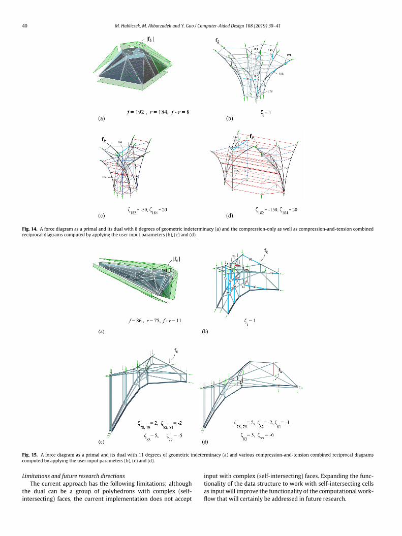
In Fig. 13b,c, the values of q are all positive which results in acompression-only solution; whereas in Fig. 13d–f, the values area combination of positive and negative resulting in systems withcombinations of both tensile and compressive forces for the sameinput force diagram. Figs. 14 and 15 also show the method usedto calculate the dual from an input force diagram where the userchanges the values of ζ and calculates various family of solutionswith both tensile and compressive internal forces. Therefore, thealgebraicmethod allows us to explore a variety of spatial structuralforms with both tensile and compressive forces without changingthe force equilibrium.

Structural analysisThe method explained in this paper can be used for both form

finding and analysis as described in Sections 2.7 and 2.8. If theprimal is considered the form, the dual will represent its forcediagram. For statically determinate cases, there will always be asingle solution (up to translation and scaling). Therefore, all theexamples used in previous sections can be used in a reverse orderas shown in Fig. 10.

For indeterminate cases, the method can be used to explorevariety of equilibrium states with various internal and externalforces. Although for statically indeterminate cases, we might beable to change the edge lengths of the dual which is the forcediagram, controlling the area of the faces and optimizing the valuesof the internal and external forces of the dual requires additionalset of constraints that were not addressed in this paper and will beinvestigated in future research.

5. Conclusions and discussions

This paper provided an algebraic formulation to construct re-ciprocal polyhedral diagrams of 3D graphic statics. The approachcan be used to construct both form and force diagrams based onthe interpretation of the input. The paper explained the process ofdeveloping the algebraic constraints and the equilibriumequationsfor the reciprocal diagrams and provided three computationalmethods including the Moore–Penrose inverse method (MPI), theReduced Row Echelon Form (RREF) approach and the Linear pro-gramming method (LP) to solve the equilibrium equations.

The MPI method can be used to construct symmetrical recip-rocal diagrams if the primal is symmetrical; the RREF approachcan be used to identify the independent edges of the dual that al-lows generating various solutions with different edge lengths andproportions. The LP method is an excellent approach to generatecompression-only results since both MPI and RREF might result inthe dual with positive and negative edge lengths.

Additionally, the paper provides insights in determining thegeometric/static degrees of (in)determinacy of the reciprocal di-agrams. For indeterminate cases, the deliberate control of the edgelengths allows exploring andmanipulating a variety of solutions inequilibriumwithout changing the planarity of the faces and break-ing the reciprocity between two diagrams which is a significantachievement of this paper.

40 M. Hablicsek, M. Akbarzadeh and Y. Guo / Computer-Aided Design 108 (2019) 30–41

Fig. 14. A force diagram as a primal and its dual with 8 degrees of geometric indeterminacy (a) and the compression-only as well as compression-and-tension combinedreciprocal diagrams computed by applying the user input parameters (b), (c) and (d).

Fig. 15. A force diagram as a primal and its dual with 11 degrees of geometric indeterminacy (a) and various compression-and-tension combined reciprocal diagramscomputed by applying the user input parameters (b), (c) and (d).

Limitations and future research directionsThe current approach has the following limitations; although

the dual can be a group of polyhedrons with complex (self-intersecting) faces, the current implementation does not accept

input with complex (self-intersecting) faces. Expanding the func-tionality of the data structure to work with self-intersecting cellsas input will improve the functionality of the computational work-flow that will certainly be addressed in future research.

M. Hablicsek, M. Akbarzadeh and Y. Guo / Computer-Aided Design 108 (2019) 30–41 41

The algebraic formulation of this paper is capable of construct-ing a reciprocal force diagram for determinate form diagramswhich is unique (up to translation and scaling), and the areas ofthe faces represent the magnitude of the forces in the primal. Al-though in graphic statics usually designers deal with the staticallydeterminate structural system, controlling the areas of the faces ofthe dual for indeterminate primal/forms was not addressed in thispaper.

In indeterminate cases, there are multiple force distributionsto describe the equilibrium of the form, and controlling the areasof the faces of the dual allows to find the optimized solutionamong them. Constructing optimized reciprocal constructions bycontrolling the areas of the faces using algebraic approach is thenext step of this research.

The current computational methods heavily rely on precisecalculation of the rank of the equilibrium matrix. In other words,the geometric degrees of (in)determinacy of the dual complex aredetermined by the rank (r) of the equilibriummatrixA. Thus, smallaccumulation of numerical errors might result in an imprecisecalculation of r that, in turn, leads to an incorrect dual complex.

References

[1] Maxwell JC. On reciprocal figures and diagrams of forces. Phil Mag Ser 41864;27(182):250–61.

[2] Culmann K. Die Graphische Statik. Zürich: Verlag Meyer und Zeller; 1864.[3] Bow RH. Economics of construction in relation to framed structures. London:

Spon; 1873.[4] Cremona L. Graphical statics: Two treatises on the graphical calculus and

reciprocal figures in graphical statics [Beare T H, Trans.], Oxford: ClarendonPress; 1890.

[5] Wolfe WS. Graphical analysis: A text book on graphic statics. New York:McGraw-Hill Book Co. Inc.; 1921.

[6] Block P. Thrust network analysis: Exploring three-dimensional equilibrium[Ph.D. thesis], Cambridge (MA, USA): Massachusetts Institute of Technology;2009.

[7] Rippmann M, Lachauer L, Block P. Interactive vault design. Int J Space Struct2012;27(4):219–30.

[8] Van Mele T, Block P. Algebraic graph statics. Comput Aided Des 2014;53:104–16.

[9] Alic V, Åkesson D. Bi-directional algebraic graphic statics. Comput Aided Des2017;93:26–37.

[10] Rankine WJM. Principle of the equilibrium of polyhedral frames. Phil Mag Ser4 1864;27(180):92.

[11] Akbarzadeh M, Van Mele T, Block P. On the equilibrium of funicular poly-hedral frames and convex polyhedral force diagrams. Comput Aided Des2015;63:118–28.

[12] Akbarzadeh M. 3D graphic statics using reciprocal polyhedral diagrams [Ph.D.thesis], Zurich (Switzerland): ETH Zurich; 2016.

[13] Williams C, McRobie A. Graphic statics using discontinuous Airy stress func-tions. Int J Space Struct 2016;31(2–4):121–34 cited by 3.

[14] McRobie A. The geometry of structural equilibrium. R Soc Open Sci 2017;4(3):Cited by 4.

[15] Lee Juney, Mele Tom Van, Block Philippe. Disjointed force polyhedra. ComputAided Des 2018;99:11–28.

[16] AkbarzadehM, VanMele T, Block P. 3D graphic statics: Geometric constructionof global equilibrium. In: Proceedings of the international association for shelland spatial structures (IASS) symposium. 2015.

[17] Akbarzadeh M, Van Mele T, Block P. Compression-only form finding throughfinite subdivision of the external force polygon. In: Proceedings of the IASS-SLTE 2014 symposium. 2014.

[18] Konstantatou M, McRobie A. 3D graphic statics: Geometric construction ofglobal equilibrium. In: Proceedings of the international association for shelland spatial structures (IASS) symposium. 2015.

[19] Lee J, Van Mele T, Block P. Form-finding explorations through geometrictransformations and modifications of force polyhedrons. In: Proceedings ofthe international association for shell and spatial structures (IASS) symposium2016. 2016.

[20] Calladine CR. Buckminster Fuller’s ‘‘Tensegrity’’ structures andClerkMaxwell’srules for the construction of stiff frames. Int J Solids Struct 1978;14(2):161–72.

[21] Schek HJ. The force density method for form finding and computation ofgeneral networks. Comput Methods Appl Mech Engrg 1974;3(1):115–34.

[22] McNeel R. et al., Rhinoceros. NURBS Modeling for Windows: http://www.rhino3d.com. 2015.

[23] Baumgart BG. A polyhedron representation for computer vision. In: AFIPS,editor. Proceedings national computer conference. 1975. p. 589–96.

[24] Moore EH. On the reciprocal of the general algebraic matrix. Bull Amer MathSoc 1920;26(9):385–96.

[25] Penrose R. A generalized inverse for matrices. Math Proc Camb Phil Soc1955;51(3):406–13.

[26] Beghini LL, Carrion J, Beghini A, Mazurek A, Baker WF. Structural optimizationusing graphic statics. Struct Multidiscip Optim 2013;49(3):351–66.

[27] Akbarzadeh M, Hablicsek M, Guo Y. Developing algebraic constraints forreciprocal polyhedral diagrams of 3D graphic statics. In: Mueller Caitlin,Adriaenssens Sigrid, editors. Proceedings of the international association forshell and spatial structures (IASS) symposium: Creativity in structural design.Boston (US): MIT; 2018.