algebraic foundations for topological data analysis draft
TRANSCRIPT

Algebraic Foundationsfor
Topological Data AnalysisDRAFT 1 March 2022
Hal Schenck
DEPARTMENT OF MATHEMATICS AND STATISTICS, AUBURN UNIVERSITY
Email address: [email protected]

c©2021 Hal Schenck
Preface
This book is a mirror of applied topology and data analysis: it covers a wide rangeof topics, at levels of sophistication varying from the elementary (matrix algebra)to the esoteric (Grothendieck spectral sequence). My hope is that there is some-thing for everyone, from undergraduates immersed in a first linear algebra class tosophisticates investigating higher dimensional analogs of the barcode. Readers areencouraged to barhop; the goal is to give an intuitive and hands on introduction tothe topics, rather than a punctiliously precise presentation.
The notes grew out of a class taught to statistics graduate students at AuburnUniversity during the COVID summer of 2020. The book reflects that: it is writtenfor a mathematically engaged audience interested in understanding the theoreticalunderpinnings of topological data analysis. Because the field draws practitionerswith a broad range of experience, the book assumes little background at the outset.However, the advanced topics in the latter part of the book require a willingness totackle technically difficult material.
To treat the algebraic foundations of topological data analysis, we need to in-troduce a fair number of concepts and techniques, so to keep from bogging down,proofs are sometimes sketched or omitted. There are many excellent texts on upperlevel algebra and topology where additional details can be found, for example:
Algebra References Topology ReferencesAluffi [2] Fulton [76]Artin [3] Greenberg–Harper [83]
Eisenbud [70] Hatcher [91]Hungerford [93] Munkres [119]
Lang [102] Spanier [137]Rotman [132] Weibel [149]
iii
iv Preface
Techniques from linear algebra have been essential tools in data analysis from thebirth of the field, and so the book kicks off with the basics:
• Least Squares Approximation
• Covariance Matrix and Spread of Data
• Singular Value Decomposition
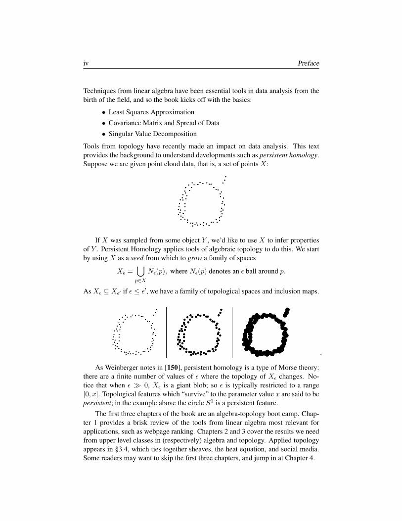
Tools from topology have recently made an impact on data analysis. This textprovides the background to understand developments such as persistent homology.Suppose we are given point cloud data, that is, a set of points X:
.
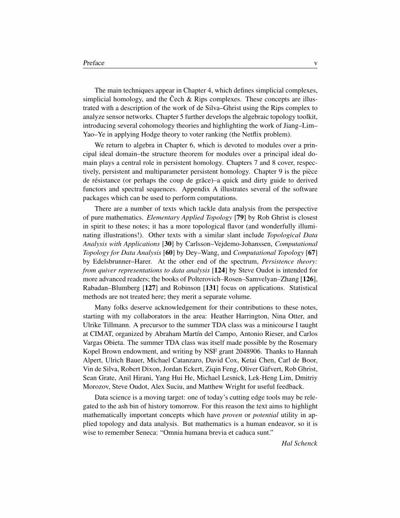
If X was sampled from some object Y , we’d like to use X to infer propertiesof Y . Persistent Homology applies tools of algebraic topology to do this. We startby using X as a seed from which to grow a family of spaces
Xε =⋃p∈X
Nε(p), where Nε(p) denotes an ε ball around p.
As Xε ⊆ Xε′ if ε ≤ ε′, we have a family of topological spaces and inclusion maps.
As Weinberger notes in [150], persistent homology is a type of Morse theory:there are a finite number of values of ε where the topology of Xε changes. No-tice that when ε 0, Xε is a giant blob; so ε is typically restricted to a range[0, x]. Topological features which “survive” to the parameter value x are said to bepersistent; in the example above the circle S1 is a persistent feature.
The first three chapters of the book are an algebra-topology boot camp. Chap-ter 1 provides a brisk review of the tools from linear algebra most relevant forapplications, such as webpage ranking. Chapters 2 and 3 cover the results we needfrom upper level classes in (respectively) algebra and topology. Applied topologyappears in §3.4, which ties together sheaves, the heat equation, and social media.Some readers may want to skip the first three chapters, and jump in at Chapter 4.
Preface v
The main techniques appear in Chapter 4, which defines simplicial complexes,simplicial homology, and the Cech & Rips complexes. These concepts are illus-trated with a description of the work of de Silva–Ghrist using the Rips complex toanalyze sensor networks. Chapter 5 further develops the algebraic topology toolkit,introducing several cohomology theories and highlighting the work of Jiang–Lim–Yao–Ye in applying Hodge theory to voter ranking (the Netflix problem).
We return to algebra in Chapter 6, which is devoted to modules over a prin-cipal ideal domain–the structure theorem for modules over a principal ideal do-main plays a central role in persistent homology. Chapters 7 and 8 cover, respec-tively, persistent and multiparameter persistent homology. Chapter 9 is the piecede resistance (or perhaps the coup de grace)–a quick and dirty guide to derivedfunctors and spectral sequences. Appendix A illustrates several of the softwarepackages which can be used to perform computations.
There are a number of texts which tackle data analysis from the perspectiveof pure mathematics. Elementary Applied Topology [79] by Rob Ghrist is closestin spirit to these notes; it has a more topological flavor (and wonderfully illumi-nating illustrations!). Other texts with a similar slant include Topological DataAnalysis with Applications [30] by Carlsson–Vejdemo-Johanssen, ComputationalTopology for Data Analysis [60] by Dey–Wang, and Computational Topology [67]by Edelsbrunner–Harer. At the other end of the spectrum, Persistence theory:from quiver representations to data analysis [124] by Steve Oudot is intended formore advanced readers; the books of Polterovich–Rosen–Samvelyan–Zhang [126],Rabadan–Blumberg [127] and Robinson [131] focus on applications. Statisticalmethods are not treated here; they merit a separate volume.
Many folks deserve acknowledgement for their contributions to these notes,starting with my collaborators in the area: Heather Harrington, Nina Otter, andUlrike Tillmann. A precursor to the summer TDA class was a minicourse I taughtat CIMAT, organized by Abraham Martın del Campo, Antonio Rieser, and CarlosVargas Obieta. The summer TDA class was itself made possible by the RosemaryKopel Brown endowment, and writing by NSF grant 2048906. Thanks to HannahAlpert, Ulrich Bauer, Michael Catanzaro, David Cox, Ketai Chen, Carl de Boor,Vin de Silva, Robert Dixon, Jordan Eckert, Ziqin Feng, Oliver Gafvert, Rob Ghrist,Sean Grate, Anil Hirani, Yang Hui He, Michael Lesnick, Lek-Heng Lim, DmitriyMorozov, Steve Oudot, Alex Suciu, and Matthew Wright for useful feedback.
Data science is a moving target: one of today’s cutting edge tools may be rele-gated to the ash bin of history tomorrow. For this reason the text aims to highlightmathematically important concepts which have proven or potential utility in ap-plied topology and data analysis. But mathematics is a human endeavor, so it iswise to remember Seneca: “Omnia humana brevia et caduca sunt.”
Hal Schenck


Contents
Preface iii
Chapter 1. Linear Algebra Tools for Data Analysis 1
§1.1. Linear Equations, Gaussian Elimination, Matrix Algebra 1
§1.2. Vector Spaces, Linear Transformations, Basis and Change of Basis 5
§1.3. Diagonalization, Webpage Ranking, Data and Covariance 8
§1.4. Orthogonality, Least Squares Fitting, Singular Value Decomposition 14
Chapter 2. Basics of Algebra: Groups, Rings, Modules 21
§2.1. Groups, Rings and Homomorphisms 21
§2.2. Modules and Operations on Modules 24
§2.3. Localization of Rings and Modules 31
§2.4. Noetherian rings, Hilbert basis theorem, Varieties 33
Chapter 3. Basics of Topology: Spaces and Sheaves 37
§3.1. Topological Spaces 38
§3.2. Vector Bundles 42
§3.3. Sheaf Theory 44
§3.4. From Graphs to Social Media to Sheaves 48
Chapter 4. Homology I: Simplicial Complexes to Sensor Networks 55
§4.1. Simplicial Complexes, Nerve of a Cover 56
§4.2. Simplicial and Singular Homology 58
§4.3. Snake Lemma and Long Exact Sequence in Homology 62
§4.4. Mayer–Vietoris, Rips and Cech complex, Sensor Networks 65
vii
viii Contents
Chapter 5. Homology II: Cohomology to Ranking Problems 73
§5.1. Cohomology: Simplicial, Cech, de Rham theories 74
§5.2. Ranking, the Netflix Problem, and Hodge Theory 80
§5.3. CW Complexes and Cellular Homology 82
§5.4. Poincare and Alexander Duality: Sensor Networks Revisited 85
Chapter 6. Persistent Algebra: Modules over a PID 95
§6.1. Principal Ideal Domains and Euclidean Domains 96
§6.2. Rational Canonical Form of a Matrix 98
§6.3. Linear Transformations, K[t]-Modules, Jordan Form 99
§6.4. Structure of Abelian Groups and Persistent Homology 100
Chapter 7. Persistent Homology 105
§7.1. Barcodes, Persistence Diagrams, Bottleneck Distance 106
§7.2. Morse Theory 114
§7.3. The Stability Theorem 117
§7.4. Interleaving and Categories 121
Chapter 8. Multiparameter Persistent Homology 131
§8.1. Definition and Examples 132
§8.2. Graded algebra, Hilbert function, series, polynomial 135
§8.3. Associated Primes and Zn-graded modules 140
§8.4. Filtrations and Ext 146
Chapter 9. Derived Functors and Spectral Sequences 151
§9.1. Injective and Projective Objects, Resolutions 152
§9.2. Derived Functors 153
§9.3. Spectral Sequences 159
§9.4. Pas de Deux: Spectral Sequences and Derived Functors 165
Appendix A. Examples of Software Packages 173
§A.1. Covariance and spread of data via R 173
§A.2. Persistent homology via scikit-tda 175
§A.3. Computational algebra via Macaulay2 179
§A.4. Multiparameter persistence via RIVET 181
Bibliography 187
Chapter 1
Linear Algebra Tools forData Analysis
We begin with a short and intense review of linear algebra. There are a numberof reasons for this approach; first and foremost is that linear algebra is the com-putational engine that drives most of mathematics, from numerical analysis (finiteelement method) to algebraic geometry (Hodge decomposition) to statistics (co-variance matrix and the shape of data). A second reason is that practitioners ofdata science come from a wide variety of backgrounds–a statistician may not haveseen eigenvalues since their undergraduate days. The goal of this chapter is todevelop basic dexterity dealing with
• Linear Equations, Gaussian Elimination, Matrix Algebra.
• Vector Spaces, Linear Transformations, Basis and Change of Basis.
• Diagonalization, Webpage Ranking, Data and Covariance.
• Orthogonality, Least Squares Data Fitting, Singular Value Decomposition.
There are entire books written on linear algebra, so our focus will be on examplesand computation, with proofs either sketched or left as exercises.
1.1. Linear Equations, Gaussian Elimination, Matrix Algebra
In this section, our goal is to figure out how to set up a system of equations to studythe following question:
Example 1.1.1. Suppose each year in Smallville that 30% of nonsmokers begin tosmoke, while 20% of smokers quit. If there are 8000 smokers and 2000 nonsmok-ers at time t = 0, after 100 years, what are the numbers? After n years? Is there anequilibrium state at which the numbers stabilize?
1
2 1. Linear Algebra Tools for Data Analysis
The field of linear algebra is devoted to analyzing questions of this type. We nowembark on a quick review of the basics. For example, consider the system of linearequations
x− 2y = 22x+ 3y = 6
Gaussian elimination provides a systematic way to manipulate the equations toreduce to fewer equations in fewer variables. A linear equation (no variable appearsto a power greater than one) in one variable is of the form x =constant, so is trivial.For the system above, we can eliminate the variable x by multiplying the first rowby −2 (note that this does not change the solutions to the system), and adding it tothe second row, yielding the new equation 7y = 2. Hence y = 2
7 , and substitutingthis for y in either of the two original equations, we solve for x, finding that x = 18
7 .Gaussian elimination is a formalization of this simple example: given a system oflinear equations
a11x1 + a12x2 + · · · a1nxn = b1a21x1 + a22x2 + · · · a2nxn = b2
......
...
(a) swap order of equations so a11 6= 0.
(b) multiply the first row by 1a11
, so the coefficient of x1 in the first row is 1.
(c) subtract ai1 times the first row from row i, for all i ≥ 2.
At the end of this process, only the first row has an equation with nonzero x1
coefficient. Hence, we have reduced to solving a system of fewer equations infewer unknowns. Iterate the process. It is important that the operations above donot change the solutions to the system of equations; they are known as elementaryrow operations: formally, these operations are
(a) Interchange two rows.
(b) Multiply a row by a nonzero constant.
(c) Add a multiple of one row to another row.
Exercise 1.1.2. Solve the system
x+ y + z = 32x+ y = 73x+ 2z = 5
You should end up with z = −75 , now backsolve. It is worth thinking about the
geometry of the solution set. Each of the three equations defines a plane in R3.What are the possible solutions to the system? If two distinct planes are parallel,we have equations ax+ by+ cz = d and ax+ by+ cz = e, with d 6= e, then thereare no solutions, since no point can lie on both planes. On the other hand, the threeplanes could meet in a single point–this occurs for the system x = y = z = 0, for
1.1. Linear Equations, Gaussian Elimination, Matrix Algebra 3
which the origin (0, 0, 0) is the only solution. Other geometric possibilities for theset of common solutions are a line or plane; describe the algebra that correspondsto the last two possibilities. There is a simple shorthand for writing a system of linear equations as above usingmatrix notation. To do so, we need to define matrix multiplication.
Definition 1.1.3. A matrix is a m × n array of elements, where m is the numberof rows and n is the number of columns.
Vectors are defined formally in §1.2; informally we think of a real vector v asan n× 1 or 1×n matrix with entries in R, and visualize it as a directed arrow withtail at the origin (0, . . . , 0) and head at the point of Rn corresponding to v.
Definition 1.1.4. The dot product of vectors v = [v1, . . . , vn] and w = [w1, . . . , wn]is
v ·w =
n∑i=1
viwi, and the length of v is |v| =√v · v.
By the law of cosines, v,w are orthogonal iff v · w = 0, which you’ll prove inExercise 1.4.1. An m × n matrix A and p × q matrix B can be multiplied whenn = p. If (AB)ij denotes the (i, j) entry in the product matrix, then
(AB)ij = rowi(A) · colj(B).
This definition may seem opaque. It is set up exactly so that when the matrix Brepresents a transition from State1 to State2 and the matrixA represents a transitionfrom State2 to State3, then the matrix AB represents the composite transition fromState1 to State3. This makes clear the reason that the number of columns ofAmustbe equal to the number of rows of B to compose the operations: the target of themap B is the source of the map A.
Exercise 1.1.5. 2 73 31 5
· [ 1 2 3 45 6 7 8
]=
37 46 55 64∗ ∗ ∗ ∗∗ ∗ ∗ ∗
Fill in the remainder of the entries. Definition 1.1.6. The transpose AT of a matrix A is defined via (AT )ij = Aji.A is symmetric if AT = A, and diagonal if Aij 6= 0 ⇒ i = j. If A and B arediagonal n× n matrices, then
AB = BA and (AB)ii = aii · biiThe n × n identiy matrix In is a diagonal matrix with 1’s on the diagonal; if A isan n×m matrix, then
In ·A = A = A · Im.An n × n matrix A is invertible if there is an n × n matrix B such that BA =AB = In. We write A−1 for the matrix B; the matrix A−1 is the inverse of A.
4 1. Linear Algebra Tools for Data Analysis
Exercise 1.1.7. Find a pair of 2 × 2 matrices (A,B) such that AB 6= BA. Showthat (AB)T = BTAT , and use this to prove that the matrix ATA is symmetric.
In matrix notation a system of n linear equations in m unknowns is written as
A · x = b, where A is an n×m matrix and x = [x1, . . . , xm]T .
We close this section by returning to our vignette.
Example 1.1.8. To start the analysis of smoking in Smallville, we write out thematrix equation representing the change during the first year, from t = 0 to t = 1.Let [n(t), s(t)]T be the vector representing the number of nonsmokers and smokers(respectively) at time t. Since 70% of nonsmokers continue as nonsmokers, and20% of smokers quit, we have n(1) = .7n(0) + .2s(0). At the same time, 30%of nonsmokers begin smoking, while 80% of smokers continue smoking, hences(1) = .3n(0) + .8s(0). We encode this compactly as the matrix equation:[
n(1)s(1)
]=
[.7 .2.3 .8
]·[n(0)s(0)
]
Now note that to compute the smoking status at t = 2, we have
[n(2)s(2)
]=
[.7 .2.3 .8
]·[n(1)s(1)
]=
[.7 .2.3 .8
]·[.7 .2.3 .8
]·[n(0)s(0)
]
And so on, ad infinitum. Hence, to understand the behavior of the system for t verylarge (written t 0), we need to compute
(limt→∞
[.7 .2.3 .8
]t)·[n(0)s(0)
]
Matrix multiplication is computationally expensive, so we’d like to find a trickto save ourselves time, energy, and effort. The solution is the following, which fornow will be a Deus ex Machina (but lovely nonetheless!) Let A denote the 2 × 2matrix above (multiply by 10 for simplicity). Then[
3/5 −2/51/5 1/5
]·[
7 23 8
]·[
1 2−1 3
]=
[5 00 10
]
Write this equation as BAB−1 = D, with D denoting the diagonal matrix onthe right hand side of the equation. An easy check shows BB−1 is the identitymatrix I2. Hence
(BAB−1)n = (BAB−1)(BAB−1)(BAB−1) · · ·BAB−1 = BAnB−1 = Dn,
1.2. Vector Spaces, Linear Transformations, Basis and Change of Basis 5
which follows from collapsing the consecutive B−1B terms in the expression. So
BAnB−1 = Dn, and therefore An = B−1DnB.
As we saw earlier, multiplying a diagonal matrix with itself costs nothing, so wehave reduced a seemingly costly computation to almost nothing; how do we find themystery matrix B? The next two sections of this chapter are devoted to answeringthis question.
1.2. Vector Spaces, Linear Transformations, Basis and Change ofBasis
In this section, we lay out the underpinnings of linear algebra, beginning with thedefinition of a vector space over a field K. A field is a type of ring, and is definedin detail in the next chapter. For our purposes, the field K will typically be one ofQ,R,C,Z/p, where p is a prime number.
Definition 1.2.1. (Informal) A vector space V is a collection of objects (vectors),endowed with two operations: vectors can be added to produce another vector, ormultiplied by an element of the field. Hence the set of vectors V is closed underthe operations. The formal definition of a vector space appears in Definition 2.2.1.
Example 1.2.2. Examples of vector spaces.
(a) V = Kn, with [a1, . . . , an] + [b1, . . . , bn] = [a1 + b1, . . . , an + bn] andc[a1, . . . , an] = [ca1, . . . , can].
(b) The set of polynomials of degree at most n − 1, with coefficients in K.Show this has the same structure as part (a).
(c) The set of continuous functions on the unit interval.
If we think of vectors as arrows, then we can visualize vector addition asputting the tail of one vector at the head of another: draw a picture to convinceyourself that
[1, 2] + [2, 4] = [3, 6].
1.2.1. Basis of a Vector Space.
Definition 1.2.3. For a vector space V , a set of vectors v1, . . . ,vk ⊆ V is
• linearly independent (or simply independent) ifk∑i=1
aivi = 0⇒ all the ai = 0.
• a spanning set for V (or simply spans V ) if for any v ∈ V there existai ∈ K such that
k∑i=1
aivi = v.
6 1. Linear Algebra Tools for Data Analysis
Example 1.2.4. The set [1, 0], [0, 1], [2, 3] is dependent, since 2·[1, 0]+3·[0, 1]−1 · [2, 3] = [0, 0]. It is a spanning set, since an arbitrary vector [a, b] = a · [1, 0] +b · [0, 1]. On the other hand, for V = K3, the set of vectors [1, 0, 0], [0, 1, 0] isindependent, but does not span.
Definition 1.2.5. A subset
S = v1, . . . ,vk ⊆ V
is a basis for V if it spans and is independent. If S is finite, we define the dimensionof V to be the cardinality of S.
A basis is loosely analogous to a set of letters for a language where the wordsare vectors. The spanning condition says we have enough letters to write everyword, while the independent condition says the representation of a word in termsof the set of letters is unique. The vector spaces we encounter in this book will befinite dimensional. A cautionary word: there are subtle points which arise whendealing with infinite dimensional vector spaces.
Exercise 1.2.6. Show that the dimension of a vector space is well defined.
1.2.2. Linear Transformations. One of the most important constructions in math-ematics is that of a mapping between objects. Typically, one wants the objects tobe of the same type, and for the map to preserve their structure. In the case ofvector spaces, the right concept is that of a linear transformation:
Definition 1.2.7. Let V and W be vector spaces. A map T : V → W is a lineartransformation if
T (cv1 + v2) = cT (v1) + T (v2),
for all vi ∈ V , c ∈ K. Put more tersely, sums split up, and scalars pull out.
While a linear transformation may seem like an abstract concept, the notion ofbasis will let us represent a linear transformation via matrix multiplication. On theother hand, our vignette about smokers in Smallville in the previous section showsthat not all representations are equal. This brings us to change of basis.
Example 1.2.8. The sets B1 = [1, 0], [1, 1] and B2 = [1, 1], [1,−1] are easilychecked to be bases for K2. Write vBi for the representation of a vector v in termsof the basis Bi. For example
[0, 1]B1 = 0 · [1, 0] + 1 · [1, 1] = 1 · [1, 1] + 0 · [1,−1] = [1, 0]B2
The algorithm to write a vector b in terms of a basis B = v1, . . . ,vn is asfollows: construct a matrix A whose columns are the vectors vi, then use Gaussianelimination to solve the system Ax = b.
Exercise 1.2.9. Write the vector [2, 1] in terms of the bases B1 and B2 above.

1.2. Vector Spaces, Linear Transformations, Basis and Change of Basis 7
To represent a linear transformation T : V → W , we need to have frames ofreference for the source and target–this means choosing bases B1 = v1, . . . ,vnfor V and B2 = w1, . . . ,wm for W . Then the matrix MB2B1 representing Twith respect to input in basisB1 and output in basisB2 has as ith column the vectorT (vi), written with respect to the basis B2. An example is in order:
Example 1.2.10. Let V = R2, and let T be the transformation that rotates a vec-tor counterclockwise by 90 degrees. With respect to the standard basis B1 =[1, 0], [0, 1], T ([1, 0]) = [0, 1] and T ([0, 1]) = [−1, 0], so
MB1B1 =
[0 −11 0
]Using the bases B1 (for input) and B2 (for output) from Example 1.2.8 yields
T ([1, 0]) = [0, 1] = 1/2 · [1, 1]− 1/2 · [1,−1]T ([1, 1]) = [−1, 1] = 0 · [1, 1]− 1 · [1,−1]
So
MB2B1 =
[1/2 0−1/2 −1
]1.2.3. Change of Basis. Suppose we have a representation of a matrix or vectorwith respect to basis B1, but need the representation with respect to basis B2. Thisis analogous to a German speaking diner being presented with a menu in French:we need a translator (or language lessons!)
Definition 1.2.11. LetB1 andB2 be two bases for the vector space V . The changeof basis matrix ∆21 takes as input a vector represented in basis B1, and outputs thesame vector represented with respect to the basis B2.
Algorithm 1.2.12. Given bases B1 = v1, . . . ,vn and B2 = w1, . . . ,wn forV , to find the change of basis matrix ∆21, form the n × 2n matrix whose first ncolumns are B2 (the “new” basis), and whose second n columns are B1 (the “old”basis). Row reduce to get a matrix whose leftmost n× n block is the identity. Therightmost n× n block is ∆21. The proof below for n = 2 generalizes easily.
Proof. Since B2 is a basis, we can write
v1 = α ·w1 + β ·w2
v2 = γ ·w1 + δ ·w2
and therefore
[ab
]B1
= a·v1+b·v2 = a·(α·w1+β ·w2)+b·(γ ·w1+δ ·w2) =([ α γ
β δ
]·[ab
])B2
8 1. Linear Algebra Tools for Data Analysis
Example 1.2.13. Let B1 = [1, 0], [0, 1] and B2 = [1, 1], [1,−1]. To find ∆12
we form the matrix [1 0 1 10 1 1 −1
]
Row reduce until the left hand block is I2, which is already the case. On the otherhand, to find ∆21 we form the matrix[
1 1 1 01 −1 0 1
]
and row reduce, yielding the matrix[1 0 1/2 1/20 1 1/2 −1/2
]
A quick check verifies that indeed[1 11 −1
]·[
1/2 1/21/2 −1/2
]=
[1 00 1
]Exercise 1.2.14. Show that the change of basis algorithm allows us to find theinverse of an n × n matrix A as follows: construct the n × 2n matrix [A|In] andapply elementary row operations. If this results in a matrix [In|B], then B = A−1,if not, then A is not invertible.
1.3. Diagonalization, Webpage Ranking, Data and Covariance
In this section, we develop the tools to analyze the smoking situation in Smallville.This will enable us to answer the questions posed earlier:
• What happens after n years?
• Is there an equilibrium state?
The key idea is that a matrix represents a linear transformation with respect to abasis, so by choosing a different basis, we may get a “better” representation. Ourgoal is to take a square matrix A and compute
limt→∞
At
So if “Tout est pour le mieux dans le meilleur des mondes possibles”, perhaps wecan find a basis where A is diagonal. Although Candide is doomed to disappoint-ment, we are not! In many situations, we get lucky, and A can be diagonalized. Totackle this, we switch from French to German.
1.3. Diagonalization, Webpage Ranking, Data and Covariance 9
1.3.1. Eigenvalues and Eigenvectors. Suppose
T : V → V
is a linear transformation; for concreteness let V = Rn. If there exists a set ofvectors B = v1, . . . ,vn with
T (vi) = λivi, with λi ∈ R,such that B is a basis for V , then the matrix MBB representing T with respect toB (which is a basis for both source and target of T ) is of the form
MBB =
λ1 0 0 0 00 λ2 0 0 0
0 0. . . 0 0
0 0 0. . . 0
0 0 0 0 λn
This is exactly what happened in Example 1.1.8, and our next task is to determinehow to find such a lucky basis. Given a matrix A representing T , we want to findvectors v and scalars λ satisfying
Av = λv or equivalently (A− λ · In) · v = 0
The kernel of a matrix M is the set of v such that M ·v = 0, so we need the kernelof (A − λ · In). Since the determinant of a square matrix is zero exactly whenthe matrix has a nonzero kernel, this means we need to solve for λ in the equationdet(A−λ ·In) = 0. The corresponding solutions are the eigenvalues of the matrixA.
Example 1.3.1. Let A be the matrix from Example 1.1.8:
det
[7− λ 2
3 8− λ
]= (7− λ)(8− λ)− 6 = λ2 − 15λ+ 50 = (λ− 5)(λ− 10).
So the eigenvalues of A are 5 and 10. These are exactly the values that appear onthe diagonal of the matrix D; as we shall see, this is no accident.
For a given eigenvalue λ, we must find some nontrivial vector v which solves(A− λ · I)v = 0; these vectors are the eigenvectors of A. For this, we go back tosolving systems of linear equations
Example 1.3.2. Staying in Smallville, we plug in our eigenvalues λ ∈ 5, 10.First we solve for λ = 5: [
7− 5 23 8− 5
]· v = 0
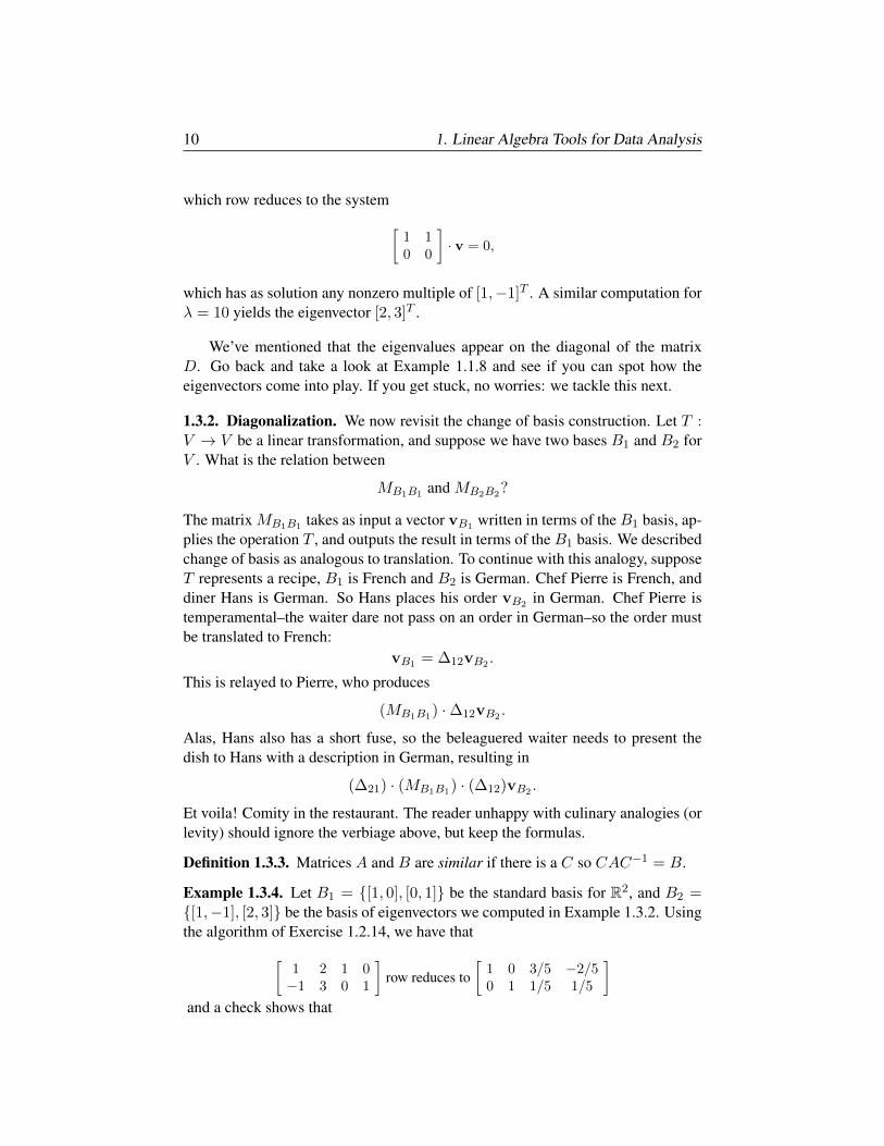
10 1. Linear Algebra Tools for Data Analysis
which row reduces to the system[1 10 0
]· v = 0,
which has as solution any nonzero multiple of [1,−1]T . A similar computation forλ = 10 yields the eigenvector [2, 3]T .
We’ve mentioned that the eigenvalues appear on the diagonal of the matrixD. Go back and take a look at Example 1.1.8 and see if you can spot how theeigenvectors come into play. If you get stuck, no worries: we tackle this next.
1.3.2. Diagonalization. We now revisit the change of basis construction. Let T :V → V be a linear transformation, and suppose we have two bases B1 and B2 forV . What is the relation between
MB1B1 and MB2B2?
The matrix MB1B1 takes as input a vector vB1 written in terms of the B1 basis, ap-plies the operation T , and outputs the result in terms of the B1 basis. We describedchange of basis as analogous to translation. To continue with this analogy, supposeT represents a recipe, B1 is French and B2 is German. Chef Pierre is French, anddiner Hans is German. So Hans places his order vB2 in German. Chef Pierre istemperamental–the waiter dare not pass on an order in German–so the order mustbe translated to French:
vB1 = ∆12vB2 .
This is relayed to Pierre, who produces
(MB1B1) ·∆12vB2 .
Alas, Hans also has a short fuse, so the beleaguered waiter needs to present thedish to Hans with a description in German, resulting in
(∆21) · (MB1B1) · (∆12)vB2 .
Et voila! Comity in the restaurant. The reader unhappy with culinary analogies (orlevity) should ignore the verbiage above, but keep the formulas.
Definition 1.3.3. Matrices A and B are similar if there is a C so CAC−1 = B.
Example 1.3.4. Let B1 = [1, 0], [0, 1] be the standard basis for R2, and B2 =[1,−1], [2, 3] be the basis of eigenvectors we computed in Example 1.3.2. Usingthe algorithm of Exercise 1.2.14, we have that[
1 2 1 0−1 3 0 1
]row reduces to
[1 0 3/5 −2/50 1 1/5 1/5
]and a check shows that
1.3. Diagonalization, Webpage Ranking, Data and Covariance 11
[3/5 −2/51/5 1/5
]·[
1 2−1 3
]= I2.
These are exactly the matrices B and B−1 which appear in Example 1.1.8. Let’scheck our computation:[
3/5 −2/51/5 1/5
]·[
7 23 8
]·[
1 2−1 3
]=
[5 00 10
]So we find
limt→∞
[.7 .2.3 .8
]t=
[1 2−1 3
]·(
limt→∞
[1/2 00 1
]t)·[
3/5 −2/51/5 1/5
]
=
[1 2−1 3
]·[
0 00 1
]·[
3/5 −2/51/5 1/5
]=
[.4 .4.6 .6
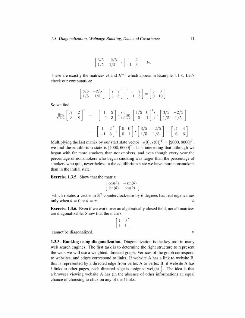
]Multiplying the last matrix by our start state vector [n(0), s(0)]T = [2000, 8000]T ,we find the equilibrium state is [4000, 6000]T . It is interesting that although webegan with far more smokers than nonsmokers, and even though every year thepercentage of nonsmokers who began smoking was larger than the percentage ofsmokers who quit, nevertheless in the equilibrium state we have more nonsmokersthan in the initial state.
Exercise 1.3.5. Show that the matrix[cos(θ) − sin(θ)sin(θ) cos(θ)
]which rotates a vector in R2 counterclockwise by θ degrees has real eigenvalues
only when θ = 0 or θ = π. Exercise 1.3.6. Even if we work over an algebraically closed field, not all matricesare diagonalizable. Show that the matrix[
1 01 1
]cannot be diagonalized. 1.3.3. Ranking using diagonalization. Diagonalization is the key tool in manyweb search engines. The first task is to determine the right structure to representthe web; we will use a weighted, directed graph. Vertices of the graph correspondto websites, and edges correspond to links. If website A has a link to website B,this is represented by a directed edge from vertex A to vertex B; if website A hasl links to other pages, each directed edge is assigned weight 1
l . The idea is thata browser viewing website A has (in the absence of other information) an equalchance of choosing to click on any of the l links.
12 1. Linear Algebra Tools for Data Analysis
From the data of a weighted, directed graph on vertices v1, . . . , vn we constructan n× n matrix T . Let lj be the number of links at vertex vj . Then
Tij =
1lj
if vertex j has a link to vertex i
0 if vertex j has no link to vertex i.
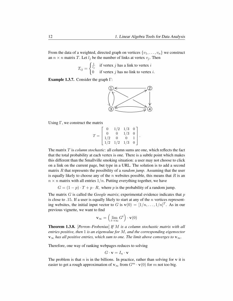
Example 1.3.7. Consider the graph Γ:
1 2
3 4
Using Γ, we construct the matrix
T =
0 1/2 1/3 00 0 1/3 0
1/2 0 0 11/2 1/2 1/3 0
.The matrix T is column stochastic: all column sums are one, which reflects the factthat the total probability at each vertex is one. There is a subtle point which makesthis different than the Smallville smoking situation: a user may not choose to clickon a link on the current page, but type in a URL. The solution is to add a secondmatrix R that represents the possibility of a random jump. Assuming that the useris equally likely to choose any of the n websites possible, this means that R is ann× n matrix with all entries 1/n. Putting everything together, we have
G = (1− p) · T + p ·R, where p is the probability of a random jump.
The matrix G is called the Google matrix; experimental evidence indicates that pis close to .15. If a user is equally likely to start at any of the n vertices represent-ing websites, the initial input vector to G is v(0) = [1/n, . . . , 1/n]T . As in ourprevious vignette, we want to find
v∞ =(
limt→∞
Gt)· v(0)
Theorem 1.3.8. [Perron–Frobenius] If M is a column stochastic matrix with allentries positive, then 1 is an eigenvalue for M , and the corresponding eigenvectorv∞ has all positive entries, which sum to one. The limit above converges to v∞.
Therefore, one way of ranking webpages reduces to solving
G · v = In · vThe problem is that n is in the billions. In practice, rather than solving for v it iseasier to get a rough approximation of v∞ from Gm · v(0) for m not too big.
1.3. Diagonalization, Webpage Ranking, Data and Covariance 13
1.3.4. Data Application: Diagonalization of the Covariance Matrix. In thissection, we discuss an application of diagonalization in statistics. Suppose wehave a data sample X = p1, . . . , pk, with the points pi = (pi1, . . . , pim) ∈ Rm.How do we visualize the spread of the data? Is it concentrated in certain directions?Do large subsets cluster? Linear algebra provides one way to attack the problem.First, we need to define the covariance matrix: let µj(X) denote the mean of thejth coordinate of the points of X , and form the matrix
Nij = pij − µj(X)
The matrix N represents the original data, but with the points translated with re-spect to the mean in each coordinate.
Definition 1.3.9. The covariance matrix of X is NT ·N .
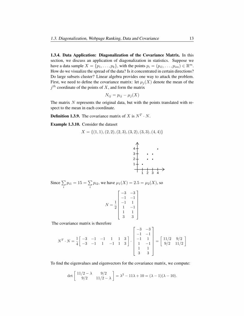
Example 1.3.10. Consider the dataset
X = (1, 1), (2, 2), (2, 3), (3, 2), (3, 3), (4, 4)
1 2 3 4
1
2
3
4
Since∑ipi1 = 15 =
∑ipi2, we have µ1(X) = 2.5 = µ2(X), so
N =1
2
−3 −3−1 −1−1 11 −11 13 3
The covariance matrix is therefore
NT ·N =1
4
[−3 −1 −1 1 1 3−3 −1 1 −1 1 3
]·
−3 −3−1 −1−1 11 −11 13 3
=
[11/2 9/29/2 11/2
]
To find the eigenvalues and eigenvectors for the covariance matrix, we compute:
det
[11/2− λ 9/2
9/2 11/2− λ
]= λ2 − 11λ+ 10 = (λ− 1)(λ− 10).
14 1. Linear Algebra Tools for Data Analysis
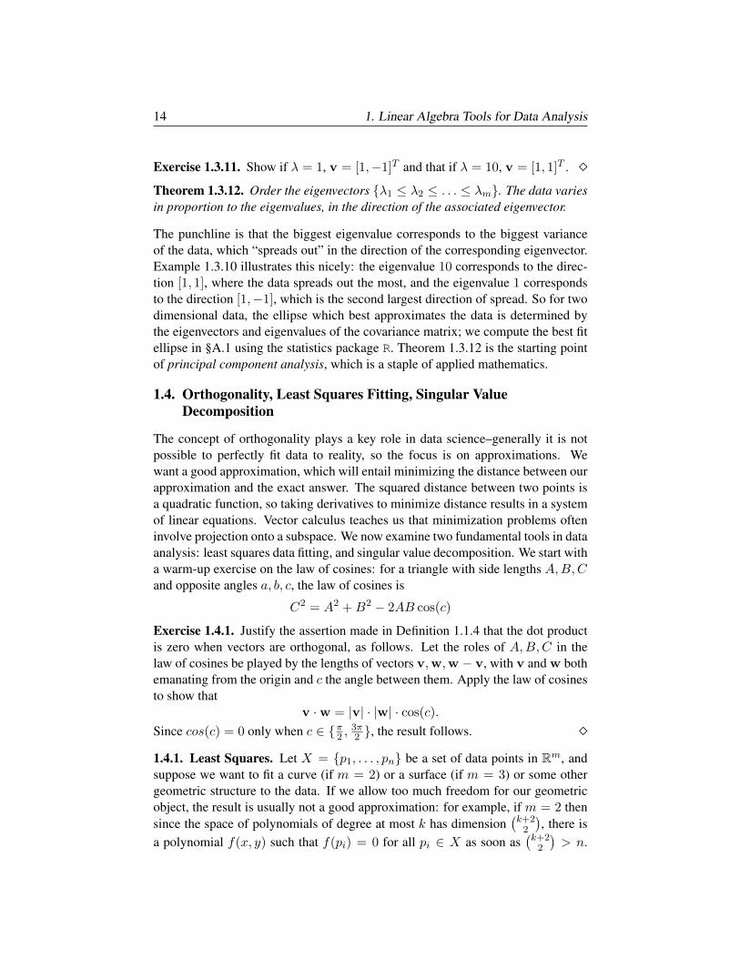
Exercise 1.3.11. Show if λ = 1, v = [1,−1]T and that if λ = 10, v = [1, 1]T . Theorem 1.3.12. Order the eigenvectors λ1 ≤ λ2 ≤ . . . ≤ λm. The data variesin proportion to the eigenvalues, in the direction of the associated eigenvector.
The punchline is that the biggest eigenvalue corresponds to the biggest varianceof the data, which “spreads out” in the direction of the corresponding eigenvector.Example 1.3.10 illustrates this nicely: the eigenvalue 10 corresponds to the direc-tion [1, 1], where the data spreads out the most, and the eigenvalue 1 correspondsto the direction [1,−1], which is the second largest direction of spread. So for twodimensional data, the ellipse which best approximates the data is determined bythe eigenvectors and eigenvalues of the covariance matrix; we compute the best fitellipse in §A.1 using the statistics package R. Theorem 1.3.12 is the starting pointof principal component analysis, which is a staple of applied mathematics.
1.4. Orthogonality, Least Squares Fitting, Singular ValueDecomposition
The concept of orthogonality plays a key role in data science–generally it is notpossible to perfectly fit data to reality, so the focus is on approximations. Wewant a good approximation, which will entail minimizing the distance between ourapproximation and the exact answer. The squared distance between two points isa quadratic function, so taking derivatives to minimize distance results in a systemof linear equations. Vector calculus teaches us that minimization problems ofteninvolve projection onto a subspace. We now examine two fundamental tools in dataanalysis: least squares data fitting, and singular value decomposition. We start witha warm-up exercise on the law of cosines: for a triangle with side lengths A,B,Cand opposite angles a, b, c, the law of cosines is
C2 = A2 +B2 − 2AB cos(c)
Exercise 1.4.1. Justify the assertion made in Definition 1.1.4 that the dot productis zero when vectors are orthogonal, as follows. Let the roles of A,B,C in thelaw of cosines be played by the lengths of vectors v,w,w − v, with v and w bothemanating from the origin and c the angle between them. Apply the law of cosinesto show that
v ·w = |v| · |w| · cos(c).
Since cos(c) = 0 only when c ∈ π2 ,3π2 , the result follows.
1.4.1. Least Squares. Let X = p1, . . . , pn be a set of data points in Rm, andsuppose we want to fit a curve (if m = 2) or a surface (if m = 3) or some othergeometric structure to the data. If we allow too much freedom for our geometricobject, the result is usually not a good approximation: for example, if m = 2 thensince the space of polynomials of degree at most k has dimension
(k+2
2
), there is
a polynomial f(x, y) such that f(pi) = 0 for all pi ∈ X as soon as(k+2
2
)> n.
1.4. Orthogonality, Least Squares Fitting, Singular Value Decomposition 15
However, this polynomial often has lots of oscillation away from the points of X .So we need to make the question more precise, and develop criteria to evaluatewhat makes a fit “good”.
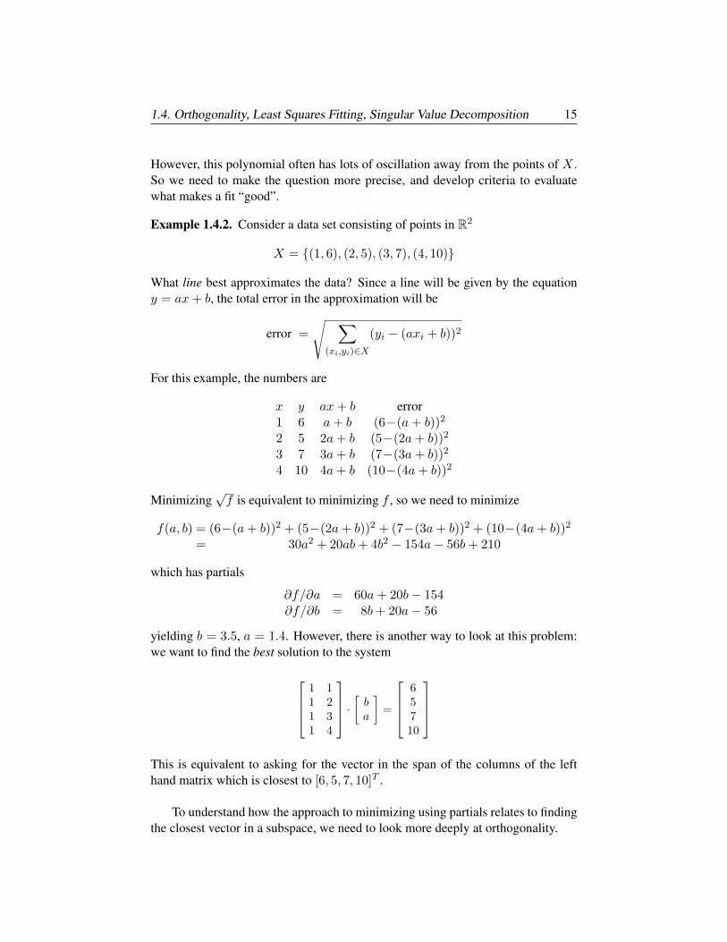
Example 1.4.2. Consider a data set consisting of points in R2
X = (1, 6), (2, 5), (3, 7), (4, 10)
What line best approximates the data? Since a line will be given by the equationy = ax+ b, the total error in the approximation will be
error =
√ ∑(xi,yi)∈X
(yi − (axi + b))2
For this example, the numbers are
x y ax+ b error1 6 a+ b (6−(a+ b))2
2 5 2a+ b (5−(2a+ b))2
3 7 3a+ b (7−(3a+ b))2
4 10 4a+ b (10−(4a+ b))2
Minimizing√f is equivalent to minimizing f , so we need to minimize
f(a, b) = (6−(a+ b))2 + (5−(2a+ b))2 + (7−(3a+ b))2 + (10−(4a+ b))2
= 30a2 + 20ab+ 4b2 − 154a− 56b+ 210
which has partials
∂f/∂a = 60a+ 20b− 154∂f/∂b = 8b+ 20a− 56
yielding b = 3.5, a = 1.4. However, there is another way to look at this problem:we want to find the best solution to the system
1 11 21 31 4
· [ ba]
=
65710
This is equivalent to asking for the vector in the span of the columns of the lefthand matrix which is closest to [6, 5, 7, 10]T .
To understand how the approach to minimizing using partials relates to findingthe closest vector in a subspace, we need to look more deeply at orthogonality.
16 1. Linear Algebra Tools for Data Analysis
1.4.2. Subspaces and orthogonality.
Definition 1.4.3. A subspace V ′ of a vector space V is a subset of V , which isitself a vector space. Subspaces W and W ′ of V are orthogonal if
w ·w′ = 0 for all w ∈W,w′ ∈W ′
A set of vectors v1, . . .vn is orthonormal if vi·vj = δij (1 if i = j, 0 otherwise).A matrix A is orthonormal when the column vectors of A are orthonormal.
Example 1.4.4. Examples of subspaces. Let A be an m× n matrix.
(a) The row space R(A) of A is the span of the row vectors of A.
(b) The column space C(A) of A is the span of the column vectors of A.
(c) The null space N(A) of A is the set of solutions to the system A · x = 0.
(d) If W is a subspace of V , then W⊥ = v|v ·w = 0 for all w ∈W.
Notice that v ∈ N(A) iff v ·w = 0 for every row vector of A.
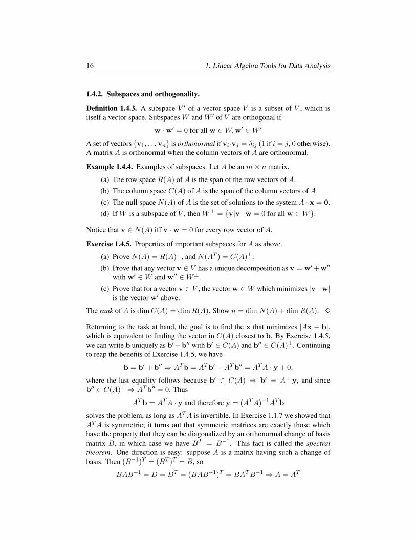
Exercise 1.4.5. Properties of important subspaces for A as above.
(a) Prove N(A) = R(A)⊥, and N(AT ) = C(A)⊥.
(b) Prove that any vector v ∈ V has a unique decomposition as v = w′+w′′
with w′ ∈W and w′′ ∈W⊥.
(c) Prove that for a vector v ∈ V , the vector w ∈W which minimizes |v−w|is the vector w′ above.
The rank of A is dimC(A) = dimR(A). Show n = dimN(A) + dimR(A). Returning to the task at hand, the goal is to find the x that minimizes |Ax − b|,which is equivalent to finding the vector in C(A) closest to b. By Exercise 1.4.5,we can write b uniquely as b′+b′′ with b′ ∈ C(A) and b′′ ∈ C(A)⊥. Continuingto reap the benefits of Exercise 1.4.5, we have
b = b′ + b′′ ⇒ ATb = ATb′ +ATb′′ = ATA · y + 0,
where the last equality follows because b′ ∈ C(A) ⇒ b′ = A · y, and sinceb′′ ∈ C(A)⊥ ⇒ ATb′′ = 0. Thus
ATb = ATA · y and therefore y = (ATA)−1ATb
solves the problem, as long as ATA is invertible. In Exercise 1.1.7 we showed thatATA is symmetric; it turns out that symmetric matrices are exactly those whichhave the property that they can be diagonalized by an orthonormal change of basismatrix B, in which case we have BT = B−1. This fact is called the spectraltheorem. One direction is easy: suppose A is a matrix having such a change ofbasis. Then (B−1)T = (BT )T = B, so
BAB−1 = D = DT = (BAB−1)T = BATB−1 ⇒ A = AT
1.4. Orthogonality, Least Squares Fitting, Singular Value Decomposition 17
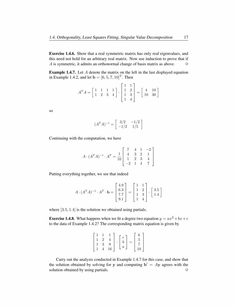
Exercise 1.4.6. Show that a real symmetric matrix has only real eigenvalues, andthis need not hold for an arbitrary real matrix. Now use induction to prove that ifA is symmetric, it admits an orthonormal change of basis matrix as above. Example 1.4.7. Let A denote the matrix on the left in the last displayed equationin Example 1.4.2, and let b = [6, 5, 7, 10]T . Then
ATA =
[1 1 1 11 2 3 4
]·
1 11 21 31 4
=
[4 1010 30
]
so
(ATA)−1 =
[3/2 −1/2−1/2 1/5
]
Continuing with the computation, we have
A · (ATA)−1 ·AT =1
10
7 4 1 −24 3 2 11 2 3 4−2 1 4 7
Putting everything together, we see that indeed
A · (ATA)−1 ·AT · b =
4.96.37.79.1
=
1 11 21 31 4
· [ 3.51.4
]
where [3.5, 1.4] is the solution we obtained using partials.
Exercise 1.4.8. What happens when we fit a degree two equation y = ax2 +bx+cto the data of Example 1.4.2? The corresponding matrix equation is given by
1 1 11 2 41 3 91 4 16
· cba
=
65710
Carry out the analysis conducted in Example 1.4.7 for this case, and show that
the solution obtained by solving for y and computing b′ = Ay agrees with thesolution obtained by using partials.
18 1. Linear Algebra Tools for Data Analysis
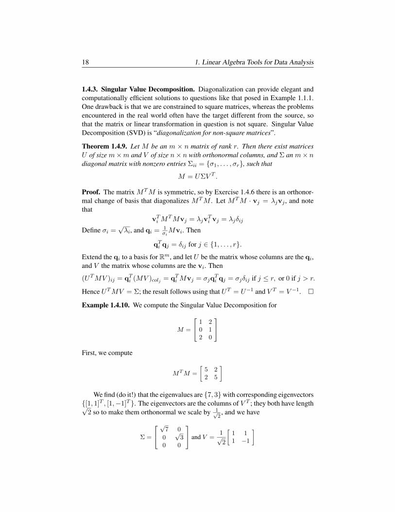
1.4.3. Singular Value Decomposition. Diagonalization can provide elegant andcomputationally efficient solutions to questions like that posed in Example 1.1.1.One drawback is that we are constrained to square matrices, whereas the problemsencountered in the real world often have the target different from the source, sothat the matrix or linear transformation in question is not square. Singular ValueDecomposition (SVD) is “diagonalization for non-square matrices”.
Theorem 1.4.9. Let M be an m × n matrix of rank r. Then there exist matricesU of size m×m and V of size n× n with orthonormal columns, and Σ an m× ndiagonal matrix with nonzero entries Σii = σ1, . . . , σr, such that
M = UΣV T .
Proof. The matrix MTM is symmetric, so by Exercise 1.4.6 there is an orthonor-mal change of basis that diagonalizes MTM . Let MTM · vj = λjvj , and notethat
vTi MTMvj = λjv
Ti vj = λjδij
Define σi =√λi, and qi = 1
σiMvi. Then
qTi qj = δij for j ∈ 1, . . . , r.
Extend the qi to a basis for Rm, and let U be the matrix whose columns are the qi,and V the matrix whose columns are the vi. Then
(UTMV )ij = qTi (MV )colj = qTi Mvj = σjqTi qj = σjδij if j ≤ r, or 0 if j > r.
Hence UTMV = Σ; the result follows using that UT = U−1 and V T = V −1.
Example 1.4.10. We compute the Singular Value Decomposition for
M =
1 20 12 0
First, we compute
MTM =
[5 22 5
]
We find (do it!) that the eigenvalues are 7, 3with corresponding eigenvectors[1, 1]T , [1,−1]T . The eigenvectors are the columns of V T ; they both have length√
2 so to make them orthonormal we scale by 1√2, and we have
Σ =
√7 0
0√
30 0
and V =1√2
[1 11 −1
]
1.4. Orthogonality, Least Squares Fitting, Singular Value Decomposition 19
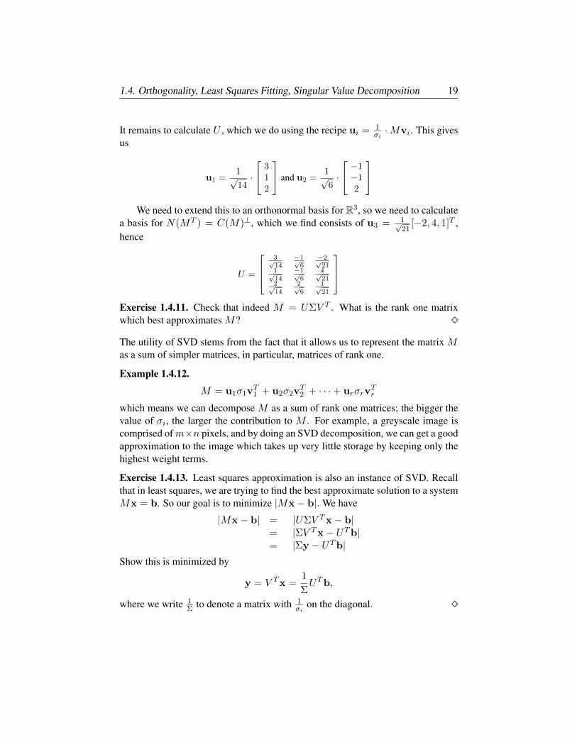
It remains to calculate U , which we do using the recipe ui = 1σi·Mvi. This gives
us
u1 =1√14·
312
and u2 =1√6·
−1−12
We need to extend this to an orthonormal basis for R3, so we need to calculate
a basis for N(MT ) = C(M)⊥, which we find consists of u3 = 1√21
[−2, 4, 1]T ,hence
U =
3√14
−1√6
−2√21
1√14
−1√6
4√21
2√14
2√6
1√21
Exercise 1.4.11. Check that indeed M = UΣV T . What is the rank one matrixwhich best approximates M? The utility of SVD stems from the fact that it allows us to represent the matrix Mas a sum of simpler matrices, in particular, matrices of rank one.
Example 1.4.12.
M = u1σ1vT1 + u2σ2v
T2 + · · ·+ urσrv
Tr
which means we can decompose M as a sum of rank one matrices; the bigger thevalue of σi, the larger the contribution to M . For example, a greyscale image iscomprised ofm×n pixels, and by doing an SVD decomposition, we can get a goodapproximation to the image which takes up very little storage by keeping only thehighest weight terms.
Exercise 1.4.13. Least squares approximation is also an instance of SVD. Recallthat in least squares, we are trying to find the best approximate solution to a systemMx = b. So our goal is to minimize |Mx− b|. We have
|Mx− b| = |UΣV Tx− b|= |ΣV Tx− UTb|= |Σy − UTb|
Show this is minimized by
y = V Tx =1
ΣUTb,
where we write 1Σ to denote a matrix with 1
σion the diagonal.

Chapter 2
Basics of Algebra: Groups,Rings, Modules
The previous chapter covered linear algebra, and in this chapter we move on tomore advanced topics in abstract algebra, starting with the concepts of group andring. In Chapter 1, we defined a vector space over a field K without giving a formaldefinition for a field; this is rectified in §1. A field is a specific type of ring, so wewill define a field in the context of a more general object. The reader has alreadyencountered many rings besides fields: the integers are a ring, as are polynomialsin one or more variables, and square matrices.
When we move into the realm of topology, we’ll encounter more exotic rings,such as differential forms. Rings bring a greater level of complexity into the pic-ture, and with that, the ability to build structures and analyze objects in finer detail.For instance, Example 2.2.8 gives a first glimpse of the objects appearing in persis-tent homology, which is the centerpiece of Chapter 7. In this chapter, we’ll cover
• Groups, Rings and Homomorphisms.
• Modules and Operations on Modules.
• Localization of Rings and Modules.
• Noetherian Rings, Hilbert Basis Theorem, Variety of an Ideal.
2.1. Groups, Rings and Homomorphisms
2.1.1. Groups. Let G be a set of elements endowed with a binary operation send-ing G×G −→ G via (a, b) 7→ a · b; in particular G is closed under the operation.The set G is a group if the following three properties hold:
• · is associative: (a · b) · c = a · (b · c).
• G possesses an identity element e such that ∀ g ∈ G, g · e = e · g = g.
• Every g ∈ G has an inverse g−1 such that g · g−1 = g−1 · g = e.
21

22 2. Basics of Algebra: Groups, Rings, Modules
The group operation is commutative if a ·b = b ·a; in this case the group is abelian.The prototypical example of an abelian group is the set of all integers, with addi-tion serving as the group operation. For abelian groups it is common to write thegroup operation as +. In a similar spirit, Z/nZ (often written Z/n for brevity) isan abelian group with group operation addition modulo n. If instead of addition inZ we attempt to use multiplication as the group operation, we run into a roadblock:zero clearly has no inverse.
For an example of a group which is not abelian, recall that matrix multiplica-tion is not commutative. The set G of n × n invertible matrices with entries in Ris a non-abelian group if n ≥ 2, with group operation matrix multiplication.
Exercise 2.1.1. Determine the multiplication table for the group of 2×2 invertiblematrices with entries in Z/2. There are 16 2×2 matrices with Z/2 entries, but anymatrix of rank zero or rank one is not a member. You should find 6 elements. Definition 2.1.2. A subgroup of a group G is a subset of G which is itself a group.A subgroup H of G is normal if gHg−1 ⊆ H for all g ∈ G, where gHg−1 is theset of elements ghg−1 for h ∈ H . A homomorphism of groups is a map which
preserves the group structure, so a map G1f−→ G2 is a homomorphism if
f(g1 · g2) = f(g1) · f(g2) for all gi ∈ Gi.
The kernel of f is the set of g ∈ G1 such that f(g) = e. If the kernel of f is ethen f is injective or one-to-one; if every g ∈ G2 has g = f(g′) for some g′ ∈ G1
then f is surjective or onto, and if f is both injective and surjective, then f is anisomorphism.
Exercise 2.1.3. First, prove that the kernel of a homomorphism is a normal sub-group. Next, let
G/H = the set of equivalence classes, with a ∼ b iff aH = bH iff ab−1 ∈ H.
Prove that the condition gHg−1 ⊆ H that defines a normal subgroup insures thatthe quotient G/H is itself a group, as long as H is normal. Exercise 2.1.4. Label the vertices of an equilateral triangle as 1, 2, 3, and con-sider the rigid motions, which are rotations by integer multiples of 2π
3 and reflectionabout any line connecting a vertex to the midpoint of the opposite edge. Prove thatthis group has 6 elements, and is isomorphic to the group in Exercise 2.1.1, as wellas to the group S3 of permutations of three letters, with the group operation in S3
given by composition: if σ(1) = 2 and τ(2) = 3, then τ · σ(1) = 3. Definition 2.1.5. There are a number of standard operations on groups:
• Direct Product and Direct Sum.
• Intersection.
• Sum (when Abelian).
2.1. Groups, Rings and Homomorphisms 23
The direct product of groupsG1 andG2 consists of pairs (g1, g2) with gi ∈ Gi, andgroup operation defined pointwiseas below; we write the direct product asG1⊕G2.
(g1, g2) · (g′1, g′2) = (g1g′1, g2g
′2).
This extends to a finite number of Gi, and in this case is also known as the directsum. To form intersection and sum, the groups G1 and G2 must be subgroups ofa larger ambient group G, and are defined as below. For the sum we will write thegroup operation additively as G1 +G2 ; the groups we encounter are all Abelian.
G1 ∩G2 = g | g ∈ G1 and g ∈ G2G1 +G2 = g1 + g2 for some gi ∈ Gi
Exercise 2.1.6. Show that the constructions in Definition 2.1.5 do yield groups. 2.1.2. Rings. A ring R is an abelian group under addition (which henceforth willalways be written as +, with additive identity written as 0), with an additional as-sociative operation multiplication (·) which is distributive with respect to addition.An additive subgroup I ⊆ R such that r · i ∈ I for all r ∈ R, i ∈ I is an ideal. Inthese notes, unless otherwise noted, rings will have
• a multiplicative identity, written as 1.
• commutative multiplication.
Example 2.1.7. Examples of rings not satisfying the above properties:
• As a subgroup of Z, the even integers 2Z satisfy the conditions above forthe usual multiplication and addition, but have no multiplicative identity.
• The set of all 2 × 2 matrices over R is an abelian group under +, has amultiplicative identity, and satisfies associativity and distributivity. Butmultiplication is not commutative.
Definition 2.1.8. A field is a commutative ring with unit 1 6= 0, such that everynonzero element has a multiplicative inverse. A nonzero element a of a ring is azero divisor if there is a nonzero element b with a · b = 0. An integral domain (forbrevity, domain) is a ring with no zero divisors.
Remark 2.1.9. General mathematical culture: a noncommutative ring such thatevery nonzero element has a left and right inverse is called a division ring. Themost famous example is the ring of quaternions, discovered by Hamilton in 1843and etched into the Brougham Bridge.
Example 2.1.10. Examples of rings.
(a) Z, the integers, and Z/nZ, the integers mod n.
(b) A[x1, . . . , xn], the polynomials with coefficients in a ring A.
(c) C0(R), the continuous functions on R.
(d) K a field.
24 2. Basics of Algebra: Groups, Rings, Modules
Definition 2.1.11. IfR and S are rings, a map φ : R→ S is a ring homomorphismif it respects the ring operations: for all r, r′ ∈ R,
(a) φ(r · r′) = φ(r) · φ(r′).
(b) φ(r + r′) = φ(r) + φ(r′).
(c) φ(1) = 1.
Example 2.1.12. There is no ring homomorphism from
Z/2 φ−→ Z.
To see this, note that in Z/2 the zero element is 2. Hence in Z we would have
0 = φ(2) = φ(1) + φ(1) = 1 + 1 = 2
An important construction is that of the quotient ring:
Definition 2.1.13. Let I ⊆ R be an ideal. Elements of the quotient ring R/I areequivalence classes, with (r + [I]) ∼ (r′ + [I]) if r − r′ ∈ I .
(r + [I]) · (r′ + [I]) = r · r′ + [I](r + [I]) + (r′ + [I]) = r + r′ + [I]
Note a contrast with the construction of a quotient group: for H a subgroup of G,G/H is itself a group only when H is a normal subgroup. There is not a similarconstraint on a ring quotient, because the additive operation in a ring is commu-tative, so all additive subgroups of R (in particular, ideals) are abelian, hence arenormal subgroups with respect to the additive structure.
Exercise 2.1.14. Prove the kernel of a ring homomorphism is an ideal.
2.2. Modules and Operations on Modules
In linear algebra, we can add two vectors together, or multiply a vector by anelement of the field over which the vector space is defined. Module is to ring whatvector space is to field. We saw above that a field is a special type of ring; a moduleover a field is a vector space. We generally work with commutative rings; if this isnot the case (e.g. tensor and exterior algebras) we make note of the fact.
Definition 2.2.1. A module M over a ring R is an abelian group, together with anaction of R on M which is R-linear: for ri ∈ R, mi ∈M ,
• r1(m1 +m2) = r1m1 + r1m2,
• (r1 + r2)m1 = r1m1 + r2m1,
• r1(r2m1) = (r1r2)m1,
• 1 · (m) = m.
• 0 · (m) = 0.
2.2. Modules and Operations on Modules 25
An R-module M is finitely-generated if there exist S = m1, . . . ,mn ⊆M suchthat any m ∈M can be written
m =n∑i=1
rimi
for some ri ∈ R. We write 〈m1, . . . ,mn〉 to denote that S is a set of generators.
Exercise 2.2.2. A subset N ⊆M of an R-module M is a submodule if N is itselfan R-module; a submodule I ⊆ R is called an ideal. Which sets below are ideals?
(a) f ∈ C0(R) | f(1) = 0.(b) f ∈ C0(R) | f(1) 6= 0.(c) n ∈ Z | n = 0 mod 3.(d) n ∈ Z | n 6= 0 mod 3.
Example 2.2.3. Examples of modules over a ring R.
(a) Any ring is a module over itself.
(b) A quotient ring R/I is both an R-module and an R/I-module.
(c) An R-module M is free if it is free of relations among a minimal set ofgenerators, so a finitely generated freeR-module is isomorphic toRn. Anideal with two or more generators is not free: if I = 〈f, g〉 then we havethe trivial (or Koszul) relation f · g − g · f = 0 on I . For modules M andN , Definition 2.1.5 shows we can construct a new module via the directsum M ⊕N . If M,N ⊆ P we also have modules M ∩N and M +N .
Definition 2.2.4. Let M1 and M2 be modules over R, mi ∈ Mi, r ∈ R. Ahomomorphism of R-modules ψ : M1 →M2 is a function ψ such that
(a) ψ(m1 +m2) = ψ(m1) + ψ(m2).
(b) ψ(r ·m1) = r · ψ(m1).
Notice that when R = K, these two conditions are exactly those for a linear trans-formation, again highlighting that module is to ring as vector space is to field.
Definition 2.2.5. LetM1
φ−→M2
be a homomorphism of R-modules.
• The kernel ker(φ) of φ consists of those m1 ∈M1 such that φ(m1) = 0.
• The image im(φ) of φ consists of those m2 ∈M2 such that m2 = φ(m1)for some m1 ∈M1.
• The cokernel coker(φ) of φ consists of M2/im(M1).
Exercise 2.2.6. Prove that the kernel, image, and cokernel of a homomorphism ofR-modules are all R-modules.
26 2. Basics of Algebra: Groups, Rings, Modules
Definition 2.2.7. A sequence of R–modules and homomorphisms
(2.2.1) C : · · ·φj+2 // Mj+1
φj+1 // Mj
φj // Mj−1
φj−1 // · · ·
is a complex (or chain complex) if
im(φj+1) ⊆ ker(φj).
The sequence is exact at Mj if im(φj+1) = ker(φj); a complex which is exacteverywhere is called an exact sequence. The jth homology module of C is:
Hj(C ) = ker(φj)/im(φj+1).
An exact sequence of the form
(2.2.2) C : 0 // A2d2 // A1
d1 // A0// 0
is called a short exact sequence.
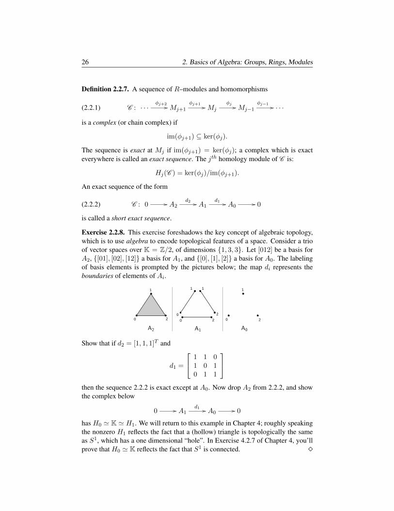
Exercise 2.2.8. This exercise foreshadows the key concept of algebraic topology,which is to use algebra to encode topological features of a space. Consider a trioof vector spaces over K = Z/2, of dimensions 1, 3, 3. Let [012] be a basis forA2, [01], [02], [12] a basis for A1, and [0], [1], [2] a basis for A0. The labelingof basis elements is prompted by the pictures below; the map di represents theboundaries of elements of Ai.
1 11 1
22 2
20000
Show that if d2 = [1, 1, 1]T and
d1 =
1 1 01 0 10 1 1
then the sequence 2.2.2 is exact except at A0. Now drop A2 from 2.2.2, and showthe complex below
0 // A1d1 // A0
// 0
has H0 ' K ' H1. We will return to this example in Chapter 4; roughly speakingthe nonzero H1 reflects the fact that a (hollow) triangle is topologically the sameas S1, which has a one dimensional “hole”. In Exercise 4.2.7 of Chapter 4, you’llprove that H0 ' K reflects the fact that S1 is connected.

2.2. Modules and Operations on Modules 27
2.2.1. Ideals. The most commonly encountered modules are ideals, which aresubmodules of the ambient ring R. An ideal I ⊆ R is proper if I 6= R.
Definition 2.2.9. Types of proper ideals I
(a) I is principal if I can be generated by a single element.
(b) I is prime if f · g ∈ I implies either f or g is in I .
(c) I is maximal if there is no proper ideal J with I ( J .
(d) I is primary if f · g ∈ I ⇒ f or gm is in I , for some m ∈ N.
(e) I is reducible if there exist ideals J1, J2 such that I = J1 ∩ J2, I ( Ji.
(f) I is radical if fm ∈ I (m ∈ N = Z>0) implies f ∈ I .
Exercise 2.2.10. Which classes above do the ideals I ⊆ R[x, y] below belong to?
(a) 〈xy〉(b) 〈y − x2, y − 1〉(c) 〈y, x2 − 1, x5 − 1〉(d) 〈y − x2, y2 − yx2 + xy − x3〉(e) 〈xy, x2〉
Hint: draw a picture of corresponding solution set in R2. If I ⊆ R is an ideal, then properties of I are often reflected in the structure of
the quotient ring R/I .
Theorem 2.2.11.R/I is a domain ⇐⇒ I is a prime ideal.R/I is a field ⇐⇒ I is a maximal ideal.
Proof. For the first part, R/I is a domain iff there are no zero divisors, hencea · b = 0 implies a = 0 or b = 0. If a and b are representatives in R of a and b,then a · b = 0 in R/I is equivalent to
ab ∈ I ⇐⇒ a ∈ I or b ∈ I,which holds iff I is prime. For the second part, suppose R/I is a field, but I is nota maximal ideal, so there exists a proper ideal J satisfying
I ⊂ J ⊆ R.Take j ∈ J . Since R/I is a field, there exists j′ such that
(j′ + [I]) · (j + [I]) = 1 which implies jj′ + (j + j′)[I] + [I] = 1.
But (j + j′)[I] + [I] = 0 in R/I , so jj′ = 1 in R/I , hence J is not a proper ideal,a contradiction.
Exercise 2.2.12. A local ring is a ring with a unique maximal ideal m. Prove thatin a local ring, if f 6∈ m, then f is an invertible element (also called a unit).
28 2. Basics of Algebra: Groups, Rings, Modules
Exercise 2.2.13. A ring is a Principal Ideal Domain (PID) if it is an integral do-main, and every ideal is principal. In Chapter 6, we will use the Euclidean algo-rithm to show that K[x] is a PID. Find a generator for
〈x4 − 1, x3 − 3x2 + 3x− 1〉.
Is K[x, y] a PID? 2.2.2. Tensor product. From the viewpoint of the additive structure, a module isjust an abelian group, hence the operations of intersection, sum, and direct sumthat we defined for groups can be carried out for modules M1 and M2 over a ringR. When M1 is a module over R1 and M2 is a module over R2, a homomorphism
R1φ−→ R2
allows us to give M2 the structure of an R1-module via
r1 ·m2 = φ(r1) ·m2.
We can also use φ to make M1 into an R2-module via tensor product.
Definition 2.2.14. Let M and N be R-modules, and let P be the free R-modulegenerated by (m,n)|m ∈ M,n ∈ N. Let Q be the submodule of P generatedby
(m1 +m2, n)− (m1, n)− (m2, n)(m,n1 + n2)− (m,n1)− (m,n2)
(rm, n)− r(m,n)(m, rn)− r(m,n).
The tensor product is the R-module:
M ⊗R N = P/Q.
We write m⊗ n to denote the class (m,n).
This seems like a strange construction, but with a bit of practice, tensor prod-uct constructions become very natural. The relations (rm, n) ∼ r(m,n) and(m, rn) ∼ r(m,n) show that tensor product is R-linear.
Example 2.2.15. For a vector space V over K , the tensor algebra T (V ) is a non-commutative ring, constructed iteratively as follows. Let V i = V ⊗ V ⊗ · · · ⊗ Vbe the i-fold tensor product, with V 0 = K. Then
T (V ) =⊕i
V i
is the tensor algebra. The symmetric algebra Sym(V ) is obtained by quotientingT (V ) by the relation vi⊗vj−vj⊗vi = 0. When V = Kn, Sym(V ) is isomorphicto the polynomial ring K[x1, . . . , xn]. The exterior algebra Λ(V ) is defined insimilar fashion, except that we quotient by the relation is vi ⊗ vj + vj ⊗ vi = 0.
2.2. Modules and Operations on Modules 29
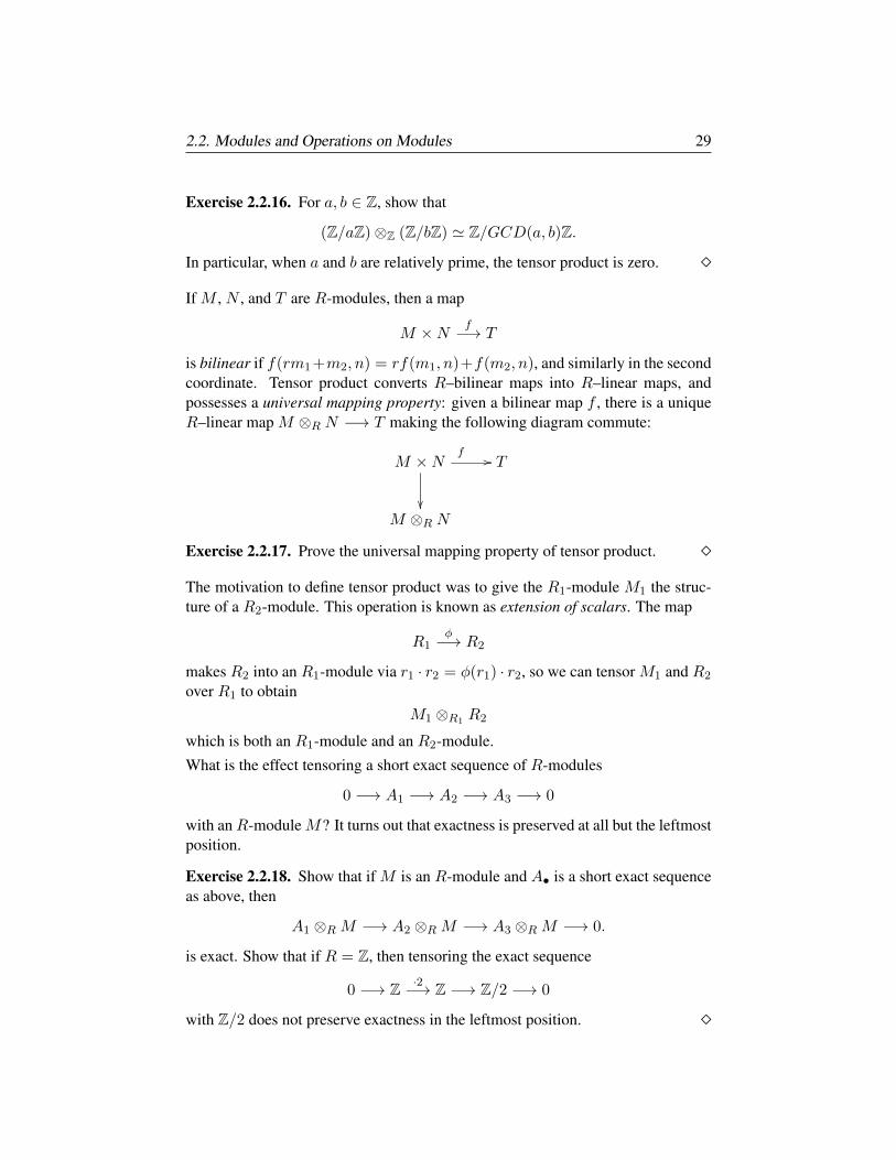
Exercise 2.2.16. For a, b ∈ Z, show that
(Z/aZ)⊗Z (Z/bZ) ' Z/GCD(a, b)Z.
In particular, when a and b are relatively prime, the tensor product is zero.
If M , N , and T are R-modules, then a map
M ×N f−→ T
is bilinear if f(rm1 +m2, n) = rf(m1, n)+f(m2, n), and similarly in the secondcoordinate. Tensor product converts R–bilinear maps into R–linear maps, andpossesses a universal mapping property: given a bilinear map f , there is a uniqueR–linear map M ⊗R N −→ T making the following diagram commute:
M ×Nf //
T
M ⊗R N
Exercise 2.2.17. Prove the universal mapping property of tensor product.
The motivation to define tensor product was to give the R1-module M1 the struc-ture of a R2-module. This operation is known as extension of scalars. The map
R1φ−→ R2
makes R2 into an R1-module via r1 · r2 = φ(r1) · r2, so we can tensor M1 and R2
over R1 to obtainM1 ⊗R1 R2
which is both an R1-module and an R2-module.
What is the effect tensoring a short exact sequence of R-modules
0 −→ A1 −→ A2 −→ A3 −→ 0
with anR-moduleM? It turns out that exactness is preserved at all but the leftmostposition.
Exercise 2.2.18. Show that if M is an R-module and A• is a short exact sequenceas above, then
A1 ⊗RM −→ A2 ⊗RM −→ A3 ⊗RM −→ 0.
is exact. Show that if R = Z, then tensoring the exact sequence
0 −→ Z ·2−→ Z −→ Z/2 −→ 0
with Z/2 does not preserve exactness in the leftmost position.
30 2. Basics of Algebra: Groups, Rings, Modules
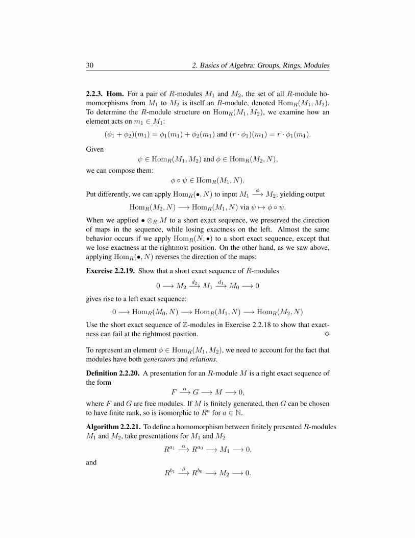
2.2.3. Hom. For a pair of R-modules M1 and M2, the set of all R-module ho-momorphisms from M1 to M2 is itself an R-module, denoted HomR(M1,M2).To determine the R-module structure on HomR(M1,M2), we examine how anelement acts on m1 ∈M1:
(φ1 + φ2)(m1) = φ1(m1) + φ2(m1) and (r · φ1)(m1) = r · φ1(m1).
Givenψ ∈ HomR(M1,M2) and φ ∈ HomR(M2, N),
we can compose them:φ ψ ∈ HomR(M1, N).
Put differently, we can apply HomR(•, N) to input M1φ−→M2, yielding output
HomR(M2, N) −→ HomR(M1, N) via ψ 7→ φ ψ.
When we applied • ⊗R M to a short exact sequence, we preserved the directionof maps in the sequence, while losing exactness on the left. Almost the samebehavior occurs if we apply HomR(N, •) to a short exact sequence, except thatwe lose exactness at the rightmost position. On the other hand, as we saw above,applying HomR(•, N) reverses the direction of the maps:
Exercise 2.2.19. Show that a short exact sequence of R-modules
0 −→M2d2−→M1
d1−→M0 −→ 0
gives rise to a left exact sequence:
0 −→ HomR(M0, N) −→ HomR(M1, N) −→ HomR(M2, N)
Use the short exact sequence of Z-modules in Exercise 2.2.18 to show that exact-ness can fail at the rightmost position. To represent an element φ ∈ HomR(M1,M2), we need to account for the fact thatmodules have both generators and relations.
Definition 2.2.20. A presentation for an R-module M is a right exact sequence ofthe form
Fα−→ G −→M −→ 0,
where F and G are free modules. If M is finitely generated, then G can be chosento have finite rank, so is isomorphic to Ra for a ∈ N.
Algorithm 2.2.21. To define a homomorphism between finitely presentedR-modulesM1 and M2, take presentations for M1 and M2
Ra1 α−→ Ra0 −→M1 −→ 0,
andRb1
β−→ Rb0 −→M2 −→ 0.
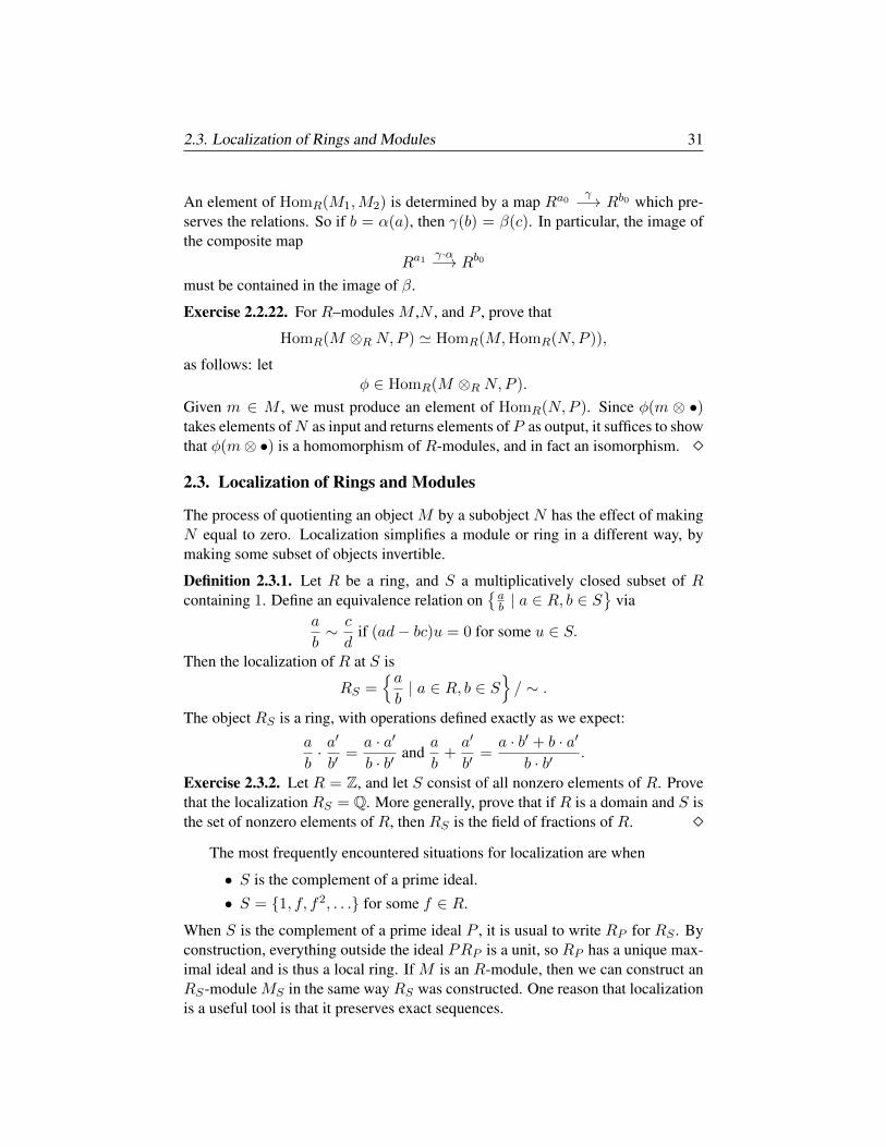
2.3. Localization of Rings and Modules 31
An element of HomR(M1,M2) is determined by a map Ra0γ−→ Rb0 which pre-
serves the relations. So if b = α(a), then γ(b) = β(c). In particular, the image ofthe composite map
Ra1γ·α−→ Rb0
must be contained in the image of β.
Exercise 2.2.22. For R–modules M ,N , and P , prove that
HomR(M ⊗R N,P ) ' HomR(M,HomR(N,P )),
as follows: letφ ∈ HomR(M ⊗R N,P ).
Given m ∈ M , we must produce an element of HomR(N,P ). Since φ(m ⊗ •)takes elements ofN as input and returns elements of P as output, it suffices to showthat φ(m⊗ •) is a homomorphism of R-modules, and in fact an isomorphism.
2.3. Localization of Rings and Modules
The process of quotienting an object M by a subobject N has the effect of makingN equal to zero. Localization simplifies a module or ring in a different way, bymaking some subset of objects invertible.
Definition 2.3.1. Let R be a ring, and S a multiplicatively closed subset of Rcontaining 1. Define an equivalence relation on
ab | a ∈ R, b ∈ S
via
a
b∼ c
dif (ad− bc)u = 0 for some u ∈ S.
Then the localization of R at S is
RS =ab| a ∈ R, b ∈ S
/ ∼ .
The object RS is a ring, with operations defined exactly as we expect:
a
b· a′
b′=a · a′
b · b′and
a
b+a′
b′=a · b′ + b · a′
b · b′.
Exercise 2.3.2. Let R = Z, and let S consist of all nonzero elements of R. Provethat the localization RS = Q. More generally, prove that if R is a domain and S isthe set of nonzero elements of R, then RS is the field of fractions of R.
The most frequently encountered situations for localization are when
• S is the complement of a prime ideal.
• S = 1, f, f2, . . . for some f ∈ R.
When S is the complement of a prime ideal P , it is usual to write RP for RS . Byconstruction, everything outside the ideal PRP is a unit, so RP has a unique max-imal ideal and is thus a local ring. If M is an R-module, then we can construct anRS-module MS in the same way RS was constructed. One reason that localizationis a useful tool is that it preserves exact sequences.
32 2. Basics of Algebra: Groups, Rings, Modules
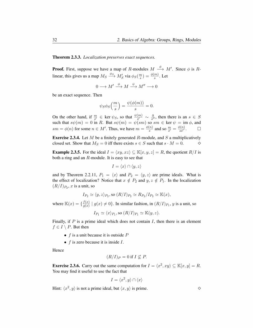
Theorem 2.3.3. Localization preserves exact sequences.
Proof. First, suppose we have a map of R-modules Mφ−→ M ′. Since φ is R-
linear, this gives us a map MSφS−→M ′S via φS(ms ) = φ(m)
s . Let
0 −→M ′φ−→M
ψ−→M ′′ −→ 0
be an exact sequence. Then
ψSφS
(ms
)=ψ(φ(m))
s= 0.
On the other hand, if ms′ ∈ ker ψS , so that ψ(m)
s′ ∼ 0s′′ , then there is an s ∈ S
such that sψ(m) = 0 in R. But sψ(m) = ψ(sm) so sm ∈ ker ψ = im φ, andsm = φ(n) for some n ∈M ′. Thus, we have m = φ(n)
s and so ms′ = φ(n)
ss′ .
Exercise 2.3.4. Let M be a finitely generated R-module, and S a multiplicativelyclosed set. Show that MS = 0 iff there exists s ∈ S such that s ·M = 0. Example 2.3.5. For the ideal I = 〈xy, xz〉 ⊆ K[x, y, z] = R, the quotient R/I isboth a ring and an R-module. It is easy to see that
I = 〈x〉 ∩ 〈y, z〉
and by Theorem 2.2.11, P1 = 〈x〉 and P2 = 〈y, z〉 are prime ideals. What isthe effect of localization? Notice that x /∈ P2 and y, z /∈ P1. In the localization(R/I)P2 , x is a unit, so
IP2 ' 〈y, z〉P2 , so (R/I)P2 ' RP2/IP2 ' K(x),
where K(x) = f(x)g(x) | g(x) 6= 0. In similar fashion, in (R/I)P1 , y is a unit, so
IP1 ' 〈x〉P1 , so (R/I)P1 ' K(y, z).
Finally, if P is a prime ideal which does not contain I , then there is an elementf ∈ I \ P . But then
• f is a unit because it is outside P
• f is zero because it is inside I .
Hence(R/I)P = 0 if I 6⊆ P.
Exercise 2.3.6. Carry out the same computation for I = 〈x2, xy〉 ⊆ K[x, y] = R.You may find it useful to use the fact that
I = 〈x2, y〉 ∩ 〈x〉
Hint: 〈x2, y〉 is not a prime ideal, but 〈x, y〉 is prime.
2.4. Noetherian rings, Hilbert basis theorem, Varieties 33
2.4. Noetherian rings, Hilbert basis theorem, Varieties
Exercise 2.2.13 defined a principal ideal domain; the ring K[x] of polynomials inone variable with coefficients in a field is an example. In particular, every ideal I ⊆K[x] can be generated by a single element, hence the question of when f(x) ∈ Iis easy to solve: find the generator g(x) for I , and check if g(x)|f(x). While thisis easy in the univariate case, in general the ideal membership problem is difficult.The class of Noetherian rings includes all principal ideal domains, but is muchlarger; in a Noetherian ring every ideal is finitely generated. Grobner bases andthe Buchberger algorithm are analogs of Gaussian Elimination for polynomials ofdegree larger than one, and provide a computational approach to tackle the idealmembership question. For details on this, see [47].
2.4.1. Noetherian Rings.
Definition 2.4.1. A ring is Noetherian if it contains no infinite ascending chains ofideals: there is no infinite chain of proper inclusions of ideals as below
I1 ( I2 ( I3 ( · · ·
A module is Noetherian if it contains no infinite ascending chains of submod-ules. A ring is Noetherian exactly when all ideals finitely generated.
Theorem 2.4.2. A ring R is Noetherian iff every ideal is finitely generated.
Proof. Suppose every ideal in R is finitely generated, but there is an infinite as-cending chain of ideals:
I1 ( I2 ( I3 ( · · ·Let J =
⋃∞i=1 Ii. Since j1 ∈ J, j2 ∈ J and r ∈ R implies j1+j2 ∈ J and r·ji ∈ J ,
J is an ideal. By assumption, J is finitely generated, say by f1, . . . , fk, and eachfi ∈ Ili for some li. So if m = maxli is the largest index, we have
Im−1 ( Im = Im+1 = · · · ,a contradiction. Now suppose that I cannot be finitely generated, so we can find asequence of elements f1, f2, . . . of I with fi 6∈ 〈f1, f2, . . . , fi−1〉. This yields
〈f1〉 ( 〈f1, f2〉 ( 〈f1, f2, f3〉 ( · · · ,which is an infinite ascending chain of ideals.
Exercise 2.4.3. Let M be a module. Prove the following are equivalent:
(a) M contains no infinite ascending chains of submodules.
(b) Every submodule of M is finitely generated.
(c) Every nonempty subset Σ of submodules of M has a maximal elementwith respect to inclusion.
The last condition says that Σ is a special type of partially ordered set.
34 2. Basics of Algebra: Groups, Rings, Modules
Exercise 2.4.4. Prove that if R is Noetherian and M is a finitely generated R-module, then M is Noetherian, as follows. Since M is finitely generated, thereexists an n such that Rn surjects onto M . Suppose there is an infinite ascendingchain of submodules of M , and consider what this would imply for R. Theorem 2.4.5. [Hilbert Basis Theorem] IfR is a Noetherian ring, then so isR[x].
Proof. Let I be an ideal in R[x]. By Theorem 2.4.2 we must show that I is finitelygenerated. The set of lead coefficients of polynomials in I generates an ideal I ′
of R, which is finitely generated, because R is Noetherian. Let I ′ = 〈g1, . . . , gk〉.For each gi there is a polynomial
fi ∈ I, fi = gixmi + terms of lower degree in x.
Let m = maxmi, and let I ′′ be the ideal generated by the fi. Given any f ∈ I ,reduce it modulo members of I ′′ until the lead term has degree less thanm. TheR-module M generated by 1, x, . . . , xm−1 is finitely generated, hence Noetherian.Therefore the submodule M ∩ I is also Noetherian, with generators h1, . . . , hj.Hence I is generated by h1, . . . , hj , g1, . . . , gk, which is a finite set.
When a ring R is Noetherian, even for an ideal I ⊆ R specified by an infiniteset of generators, there will exist a finite generating set for I . A field K is Noether-ian, so the Hilbert Basis Theorem and induction tell us that the ring K[x1, . . . , xn]is Noetherian, as is a polynomial ring over Z or any other principal ideal domain.Thus, the goal of determining a finite generating set for an ideal is attainable.
2.4.2. Solutions to a polynomial system: Varieties. In linear algebra, the objectsof study are the solutions to systems of polynomial equations of the simplest type:all polynomials are of degree one. Algebraic geometry is the study of the sets ofsolutions to systems of polynomial equations of higher degree. The choice of fieldis important: x2 + 1 = 0 has no solutions in R and two solutions in C; in linearalgebra this issue arose when computing eigenvalues of a matrix.
Definition 2.4.6. A field K is algebraically closed if every nonconstant polynomialf(x) ∈ K[x] has a solution f(p) = 0 with p ∈ K. The algebraic closure K is thesmallest field containing K which is algebraically closed.
Given a system of polynomial equations f1, . . . , fk ⊆ R = K[x1, . . . , xn], notethat the set of common solutions over K depends only on the ideal
I = 〈f1, . . . , fk〉 = k∑i=1
gifi | gi ∈ R
The set of common solutions is called the variety of I , denoted
V(I) ⊆ Kn ⊆ Kn

2.4. Noetherian rings, Hilbert basis theorem, Varieties 35
Adding more equations to a polynomial system imposes additional constraints onthe solutions, hence passing to varieties reverses inclusion
I ⊆ J ⇒ V(J) ⊆ V(I)
Since ideals I , J ⊆ R are submodules of the same ambient module, we have
• I ∩ J = f | f ∈ I and f ∈ J.• IJ = 〈fg | f ∈ I and g ∈ J〉.• I + J = f + g | f ∈ I and g ∈ J.
It is easy to check these are all ideals.
Exercise 2.4.7. Prove that
V(I ∩ J) = V(I) ∪V(J) = V(IJ)
and that V(I + J) = V(I) ∩V(J). Definition 2.4.8. The radical of an ideal I ⊆ R is
√I = f | fm ∈ I for some power m.
Exercise 2.4.9. Show if I = 〈x2−xz, xy−yz, xz−z2, xy−xz, y2−yz, yz−z2〉in K[x, y, z], then
√I = 〈x− z, y − z〉.
Definition 2.4.10. For ideals I, J ⊆ R, the ideal quotient (or colon ideal) is
I : J = f ∈ R | f · J ⊆ I.
Exercise 2.4.11. For I and√I as in Exercise 2.4.9 show I :
√I = 〈x, y, z〉.
The operations of radical and ideal quotient have geometric interpretations; wetackle the radical first. Given X ⊆ Kn, consider the set I(X) of all polynomials inR = K[x1, . . . , xn] which vanish on X .
Exercise 2.4.12. Prove that I(X) is an ideal, and in fact a radical ideal. Next,prove that V(I(X)) is the smallest variety containing X . Notice that for I = 〈x2 + 1〉 ⊆ R[x] ⊆ C[x], V(I) is empty in R, but consists oftwo points in C. This brings us Hilbert’s Nullstellensatz (see [70] for a proof).
Theorem 2.4.13. If K is algebraically closed, then
• Hilbert Nullstellensatz (Weak version): V(I) = ∅ ⇐⇒ 1 ∈ I.• Hilbert Nullstellensatz (Strong version): I(V(I)) =
√I.
An equivalent formulation is that over an algebraically closed field, there is a 1 : 1correspondence between maximal ideals I(p) and points p. For an arbitrary setX ⊆ Kn, the smallest variety containing X is V(I(X)). It is possible to define atopology, called the Zariski topology on Kn, where the closed sets are of the formV(I), and when working with this topology we write AnK and speak of affine space.
36 2. Basics of Algebra: Groups, Rings, Modules
We touch on the Zariski topology briefly in the general discussion of topologicalspaces in Chapter 3. We close with the geometry of the ideal quotient operation.Suppose we know there is some spurious or unwanted component V(J) ⊆ V(I).How do we remove V(J)? Equivalently, what is the smallest variety containingV(I) \V(J)?
Theorem 2.4.14. The variety V(I(V(I) \V(J))) ⊆ V(I : J).
Proof. Since I1 ⊆ I2 ⇒ V(I2) ⊆ V(I1), it suffices to show
I : J ⊆ I(V(I) \V(J)).
If f ∈ I : J and p ∈ V(I) \ V(J), then since p 6∈ V(J) there is a g ∈ J withg(p) 6= 0. Since f ∈ I : J , fg ∈ I , and so
p ∈ V(I)⇒ f(p)g(p) = 0.
As g(p) 6= 0, this forces f(p) = 0 and therefore f ∈ I(V(I) \V(J)).
Example 2.4.15. Projective space PnK over a field K is defined as
Kn+1 \ 0/ ∼ where p1 ∼ p2 iff p1 = λp2 for some λ ∈ K∗.One way to visualize PnK is as the set of lines through the origin in Kn+1.
Writing V(x0)c for the points where x0 6= 0, we have that Kn ' V(x0)c ⊆ PnKvia (a1, . . . , an) 7→ (1, a1, . . . , an). This can be quite useful, since PnK is compact.
Exercise 2.4.16. Show that a polynomial f =∑cαix
αi ∈ K[x0, . . . , xn] hasa well-defined zero set in PnK iff it is homogeneous: the exponents all have thesame weight. Put differently, all the αi have the same dot product with the vector[1, . . . , 1]. Show that a homogeneous polynomial f does not define a function onPnK, but that the rational function f
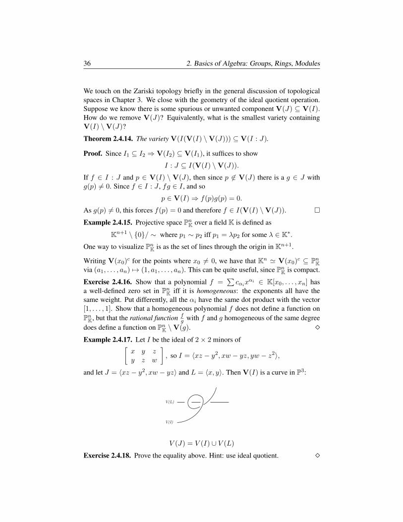
g with f and g homogeneous of the same degreedoes define a function on PnK \V(g). Example 2.4.17. Let I be the ideal of 2× 2 minors of[
x y zy z w
], so I = 〈xz − y2, xw − yz, yw − z2〉,
and let J = 〈xz − y2, xw − yz〉 and L = 〈x, y〉. Then V(I) is a curve in P3:
V (J) = V (I) ∪ V (L)
Exercise 2.4.18. Prove the equality above. Hint: use ideal quotient.
Chapter 3
Basics of Topology: Spacesand Sheaves
In Chapter we covered the basics of upper level algebra. Now we do the same thingfor topology: this chapter covers some key ideas of topology and sheaf theory. Westart in §1 with a quick review of topological basics. In §2 we discuss vectorbundles, where the central construction provides a good intuition for sheaf theory,which is introduced in §3. Sheaf theory can be a somewhat daunting topic whenfirst encountered; the main point to keep in mind is that a sheaf is really nothingmore than a bookkeeping device.
• Sheaves organize local data, assigning to every open set U an algebraicobject F (U). When V ⊆ U , there is a restriction map
F (U)ρUV−→ F (V )
satisfying several natural conditions which appear in Definition 3.3.1.
• Sheaves facilitate the construction of global structures from local struc-tures: this is often referred to as gluing, formalized in Definition 3.3.2.
The chapter concludes with a description of the work of Hansen-Ghrist applyingsheaf theory to social networks. This requires a quick introduction to spectralgraph theory, relating the graph Laplacian to the heat equation. The main idea isthat the heat equation is a good model for the spread of opinion over a social medianetwork. The topics covered in this chapter are:
• Topological Spaces.
• Vector Bundles.
• Sheaf Theory.
• Sheaves, Graphs, and Social Media.
37

38 3. Basics of Topology: Spaces and Sheaves
3.1. Topological Spaces
3.1.1. Set theory and equivalence relations. In this section we fix notation, andreview basic topology and set theory. A set S is a (not necessarily finite) collectionof elements s1, . . . , sk, . . .; standard operations among sets include
(a) union: S1 ∪ S2 = m | m ∈ S1 or m ∈ S2.(b) intersection: S1 ∩ S2 = m | m ∈ S1 and m ∈ S2.(c) set difference: S1 \ S2 = m | m ∈ S1 and m 6∈ S2.
The Cartesian product S1 × S2 of two sets is
S1 × S2 = (s1, s2) | si ∈ Siand a relation ∼ between S1 and S2 is a subset of pairs of S1 × S2. We say that arelation on S × S is
(a) reflexive if a ∼ a for all a ∈ S.
(b) symmetric if a ∼ b⇒ b ∼ a for all a, b ∈ S.
(c) transitive if a ∼ b and b ∼ c⇒ a ∼ c for all a, b, c ∈ S.
A relation which is reflexive, symmetric, and transitive is an equivalence relation.
Exercise 3.1.1. Show that an equivalence relation partitions a set into disjoint sub-sets. Each of these subsets (which consist of elements related by ∼) is called anequivalence class. A relation R ⊆ S × S is a partial order on S if it is transitive, and (s1, s2) and(s2, s1) ∈ R imply that s1 = s2. In this case S is called a poset, which is shorthandfor “partially ordered set”.
3.1.2. Definition of a topology. The usual setting for calculus and elementaryanalysis is over the real numbers; Rn is a metric space, with d(p, q) the distancebetween points p and q. A set U ⊆ Rn is open when for every p ∈ U there existsδp > 0 such that
Nδp(p) = q | d(q, p) < δp ⊆ U,and closed when the complement Rn \ U is open. The key properties of open setsare that any (including infinite) union of open sets is open, and a finite intersectionof open sets is open. Topology takes this as a cue.
Definition 3.1.2. A topology on a set S is a collection U of subsets U ⊆ S, satis-fying conditions (a)-(c) below. Elements of U are the open sets of the topology,and (S,U ) (or, for short, just S) is a topological space.
(a) ∅ and S are elements of U .
(b) U is closed under arbitrary union: for Ui ∈ U ,⋃i∈I Ui ∈ U .
(c) U is closed under finite intersection: for Ui ∈ U ,⋂mi=1 Ui ∈ U .
3.1. Topological Spaces 39
Exercise 3.1.3. Prove that a topology can also be defined by specifying the closedsets, by complementing the conditions of Definition 3.1.2. Since Rn is a metric space, the notions of distance and limit points are intuitive.How can we define limit points in the setting of an abstract topological space?
Definition 3.1.4. If S is a topological space, then p ∈ S is a limit point of X ⊆ Sif for all U ∈ U with p ∈ U ,
(U \ p) ∩X 6= ∅
The closure X of X is defined as X ∪ q | q is a limit point of X.
Definition 3.1.5. A collection B of subsets of S is a basis for the topology if everyfinite intersection of elements of B is a union of elements of B. It is not hard toshow that the collection of (arbitrary) unions of elements of B is a topology, calledthe topology generated by B.
Example 3.1.6. In Rn, B = Nδ(p) | p ∈ Rn and δ ∈ R>0 is a basis.
Our last definitions involve properties of coverings and continuity:
Definition 3.1.7. A collection U of subsets of S is a cover of S if⋃Ui∈U
Ui = S.
S is compact if every open covering admits a finite subcover, and connected if theonly sets that are both open and closed are ∅ and S.
Example 3.1.8. [Heine-Borel] A set S ⊆ Rn is compact iff it is closed andbounded.
Definition 3.1.9. Let S and T be topological spaces. A function
Sf−→ T
is continuous if f−1(U) is open in S for every open set U ⊆ T . We say that Sand T are homeomorphic if f and f−1 are 1:1 and continuous for some map f asabove. Two maps f0, f1 : S → T are homotopic if there is a continuous map
S × [0, 1]F−→ T
such that F (x, 0) = f0(x) and F (x, 1) = f1(x). F deforms the map f0 to the mapf1. The spaces S and T are homotopic if there is a map g : T → S such that f gis homotopic to 1T and g f is homotopic to 1S . We say that a topological spaceis contractible if it is homotopic to a point.
Exercise 3.1.10. Prove that if Sf−→ T is continuous and X is a compact subset
of S, then f(X) is a compact subset of T .
40 3. Basics of Topology: Spaces and Sheaves
3.1.3. Discrete, product, and quotient topologies. We now discuss some com-mon topologies, as well as how to build new topological spaces from old. Our firstexample is
Definition 3.1.11. [Discrete Topology] The topology in which every subset A of Sis open is called the discrete topology. Since the complement S \A is also a subset,this means every subset is both open and closed.
From the perspective of data science, point cloud data only comes equipped withthe discrete topology; by adding a parameter we are able to bring interesting topo-logical features into the picture in Chapter 7 with persistent homology.
Definition 3.1.12. [Product Topology]. If X1 and X2 are topological spaces, thenthe Cartesian product has a natural topology associated with it, the product topol-ogy, where open sets are unions of sets of the form U1 × U2 with Ui open in Xi.In particular, if Bi is a basis for Xi, then taking the Ui to be members of Bi showsthat B1 ×B2 is a basis for X1 ×X2.
Exercise 3.1.13. Show that the product topology is the coarsest topology–the topol-ogy with the fewest open sets–such that the projection maps
X1 ×X2
π1zz
π2
$$X1 X2
are continuous, where πi(x1, x2) = xi. Definition 3.1.14. [Induced and Quotient Topology]
• If Yi→ X then the induced topology on Y is the topology where open
sets of Y are i−1(U) for U open in X .
• Let X be a topological space and ∼ an equivalence relation. The quo-tient space Y = X/∼ is the set of equivalence classes, endowed with thequotient topology: U ⊆ Y is open iff
V = π−1(U) is open in X , where X π−→ X/∼ .
Example 3.1.15. For W ⊆ X , define an equivalence relation via
a ∼ b⇐⇒ a, b ∈W or a = b.
This collapsesW to a point, so for example ifX = [0, 1] with the induced topologyfrom R1 andW consists only of the two endpoints 0, 1 thenX/W is homeomor-phic to S1, and if X is the unit square [0, 1] × [0, 1] and W = ∂(X) then X/Y ishomeomorphic to S2. In contrast, if we define an equivalence relation on X via(x, 1) ∼ (x, 0) and (0, y) ∼ (1, y) then X/∼ is homeomorphic to the torus T 2.
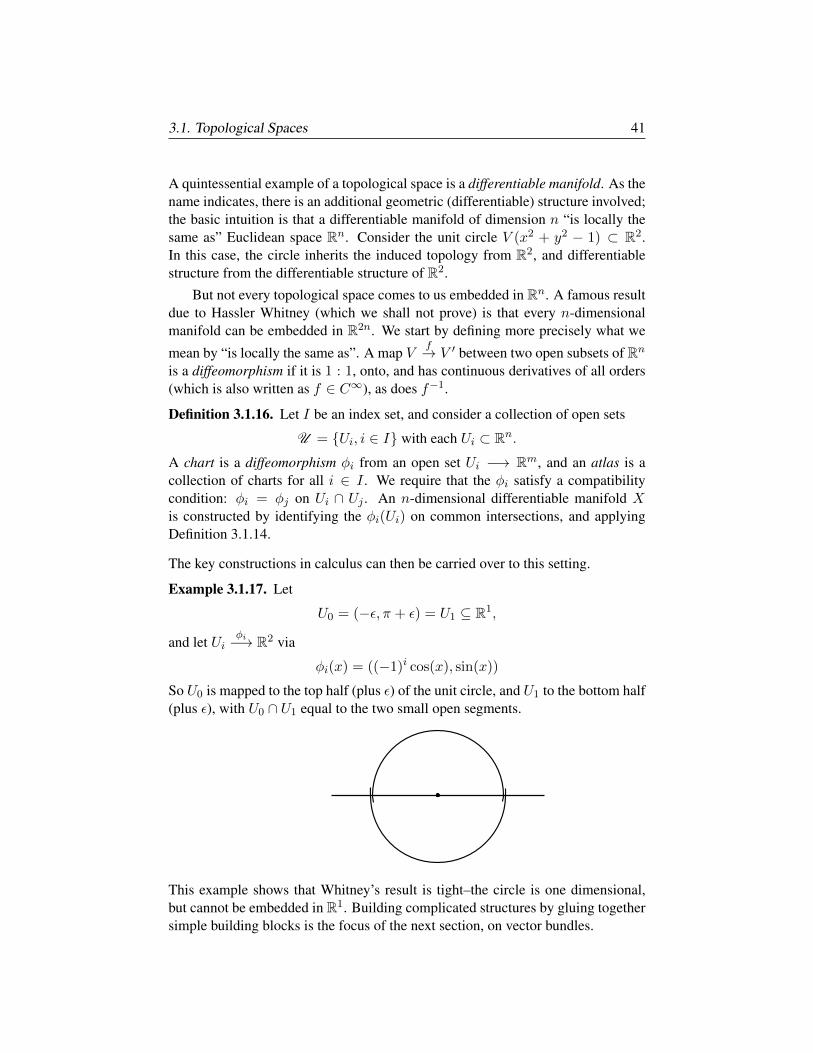
3.1. Topological Spaces 41
A quintessential example of a topological space is a differentiable manifold. As thename indicates, there is an additional geometric (differentiable) structure involved;the basic intuition is that a differentiable manifold of dimension n “is locally thesame as” Euclidean space Rn. Consider the unit circle V (x2 + y2 − 1) ⊂ R2.In this case, the circle inherits the induced topology from R2, and differentiablestructure from the differentiable structure of R2.
But not every topological space comes to us embedded in Rn. A famous resultdue to Hassler Whitney (which we shall not prove) is that every n-dimensionalmanifold can be embedded in R2n. We start by defining more precisely what we
mean by “is locally the same as”. A map Vf→ V ′ between two open subsets of Rn
is a diffeomorphism if it is 1 : 1, onto, and has continuous derivatives of all orders(which is also written as f ∈ C∞), as does f−1.
Definition 3.1.16. Let I be an index set, and consider a collection of open sets
U = Ui, i ∈ I with each Ui ⊂ Rn.A chart is a diffeomorphism φi from an open set Ui −→ Rm, and an atlas is acollection of charts for all i ∈ I . We require that the φi satisfy a compatibilitycondition: φi = φj on Ui ∩ Uj . An n-dimensional differentiable manifold Xis constructed by identifying the φi(Ui) on common intersections, and applyingDefinition 3.1.14.
The key constructions in calculus can then be carried over to this setting.
Example 3.1.17. Let
U0 = (−ε, π + ε) = U1 ⊆ R1,
and let Uiφi−→ R2 via
φi(x) = ((−1)i cos(x), sin(x))
So U0 is mapped to the top half (plus ε) of the unit circle, and U1 to the bottom half(plus ε), with U0 ∩ U1 equal to the two small open segments.
This example shows that Whitney’s result is tight–the circle is one dimensional,but cannot be embedded in R1. Building complicated structures by gluing togethersimple building blocks is the focus of the next section, on vector bundles.
42 3. Basics of Topology: Spaces and Sheaves
3.2. Vector Bundles
While vector bundles are fundamental objects in topology, the reason to includethem in these notes is that they provide the right intuition to motivate the definitionof a sheaf. In this section we work with real, topological vector bundles, wheremaps between objects are continuous, written as C0; for algebraic vector bundlessee [48]. The formal definition appears below; the intuition is that a rank n vectorbundle V on a space X is locally a product space of the form
Ui × Rn, with Ui ∈ U a cover of X,
along with projection maps V → Ui. We will also touch briefly on geometry todiscuss the tangent and cotangent bundles of a manifold, where the maps betweenobjects will be differentiable, written as C∞.
Example 3.2.1. A product space of the form X ∼= Y × Rn (where ∼= denoteshomeomorphism) is a trivial vector bundle; for example an infinite cylinder C is
C ∼= S1 × R1
A small connected open set U ⊆ S1 is homeomorphic to R1, and C can be coveredby sets of this form. On the other hand, the Mobius band M is also a rank onevector bundle on S1, and locally has the same form as C. As Exercise 3.2.5 shows,the spaces M and C are different.
Definition 3.2.2. A topological space V is a rank n vector bundle (typically calledthe total space) on a topological space X (typically called the base space) if thereis a continuous map
Vπ−→ X
such that
• There exists an open cover U = Uii∈I of X , and homeomorphisms
π−1(Ui)φi−→ Ui × Rn
such that φi followed by projection onto Ui is π, and
• The transition maps φij = φi φ−1j :
φjπ−1(Uj) ⊇ (Ui ∩ Uj)× Rn
φij−→ (Ui ∩ Uj)× Rn ⊆ φiπ−1(Ui)
satisfy φij ∈ GLn(C0(Ui ∩ Uj)).
A cover Ui so that the first bullet above holds is a trivialization, because locallya vector bundle on X looks like a product of Ui with Rn. The map φj gives us achart: a way to think of a point in π−1(Uj) as a point (t, v) ∈ Uj × Rn. The copyof Rn ∼= φiπ
−1(p) over a point p is called the fiber over p. If we change from achart over Uj to a chart over Ui, then
(t, vj) 7→ (t, [φij(t)] · vj)
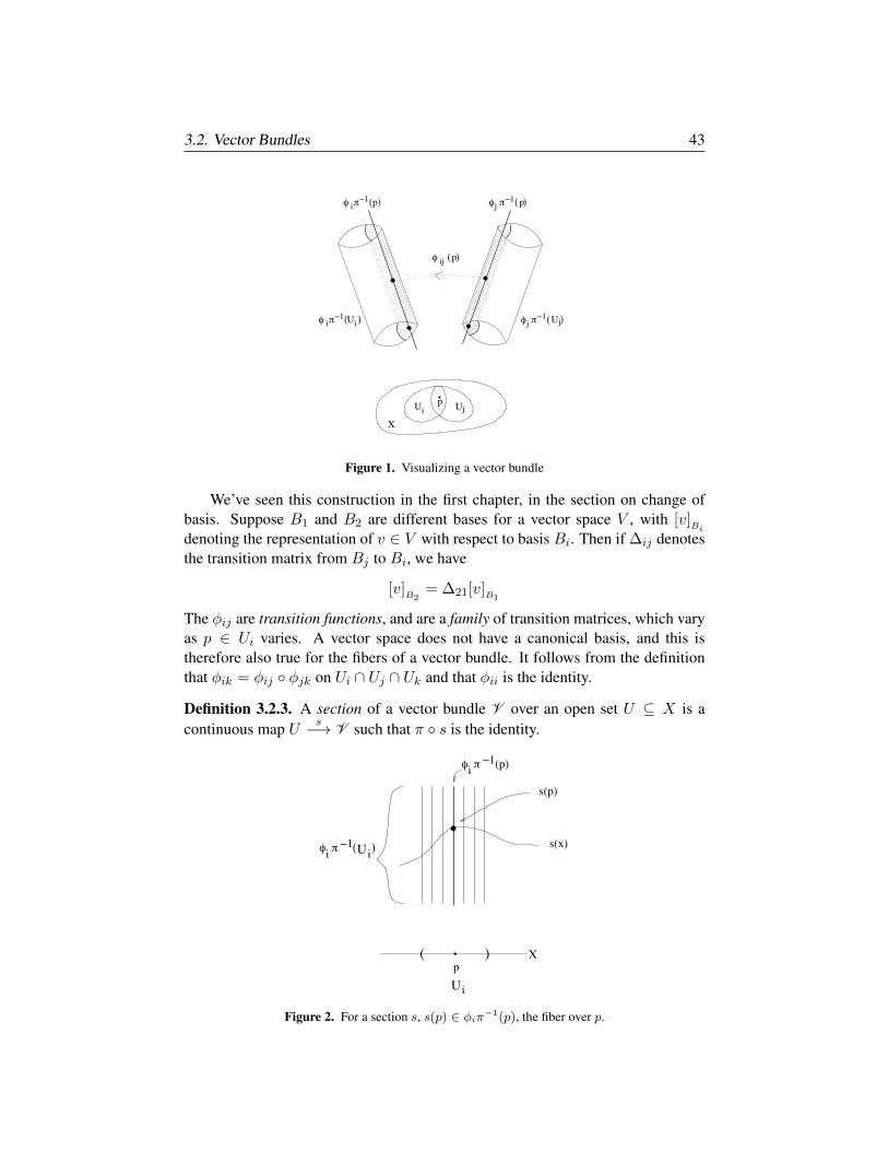
3.2. Vector Bundles 43
X
−1i
j
p
j−1φ π ( )
i
U Ui j
φ π ( )i φ π ( )−1 Uj−1
p
U
φ π ( ) p
φ ( )ij p
Figure 1. Visualizing a vector bundle
We’ve seen this construction in the first chapter, in the section on change ofbasis. Suppose B1 and B2 are different bases for a vector space V , with [v]Bidenoting the representation of v ∈ V with respect to basis Bi. Then if ∆ij denotesthe transition matrix from Bj to Bi, we have
[v]B2= ∆21[v]B1
The φij are transition functions, and are a family of transition matrices, which varyas p ∈ Ui varies. A vector space does not have a canonical basis, and this istherefore also true for the fibers of a vector bundle. It follows from the definitionthat φik = φij φjk on Ui ∩ Uj ∩ Uk and that φii is the identity.
Definition 3.2.3. A section of a vector bundle V over an open set U ⊆ X is acontinuous map U s−→ V such that π s is the identity.
p( )
s(x)
X
φ π (p)
Ui
i−1
s(p)
i U φ π ( )
−1i
Figure 2. For a section s, s(p) ∈ φiπ−1(p), the fiber over p.
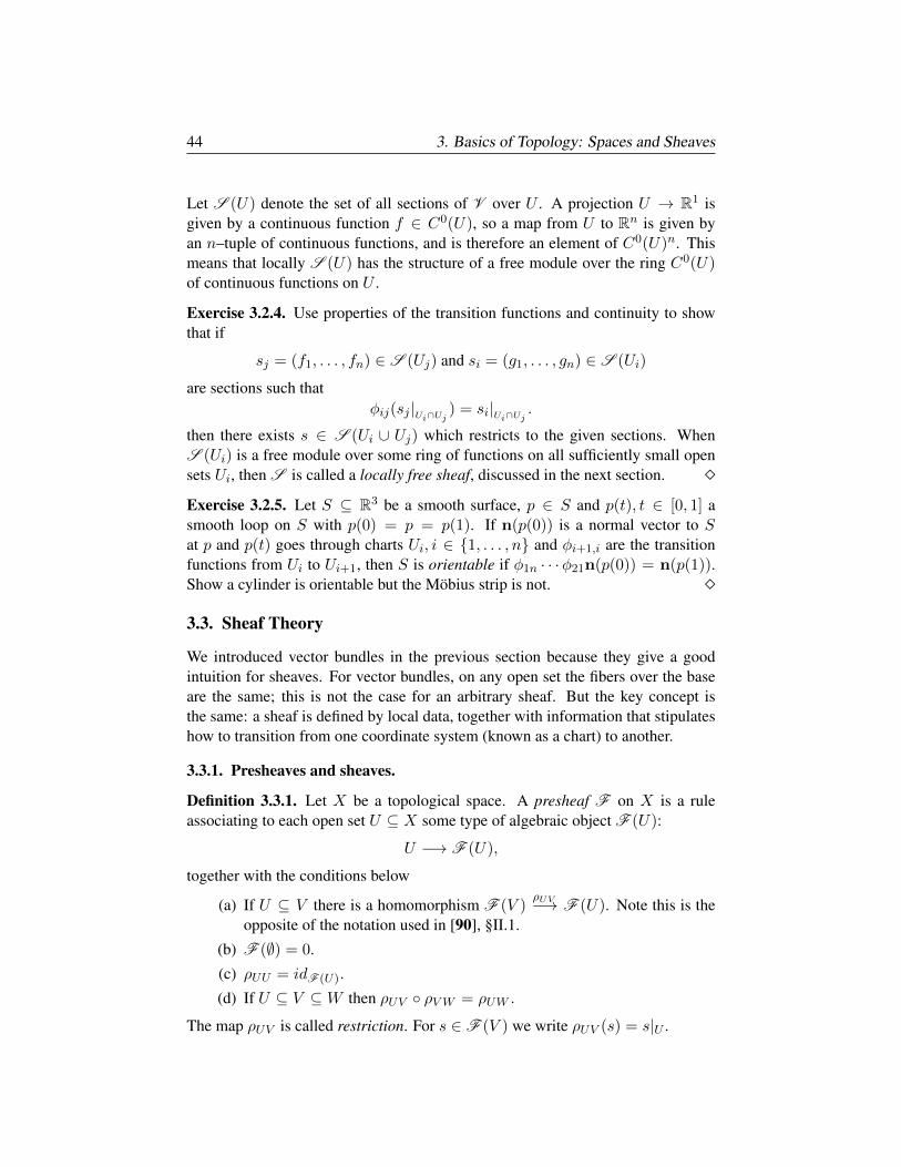
44 3. Basics of Topology: Spaces and Sheaves
Let S (U) denote the set of all sections of V over U . A projection U → R1 isgiven by a continuous function f ∈ C0(U), so a map from U to Rn is given byan n–tuple of continuous functions, and is therefore an element of C0(U)n. Thismeans that locally S (U) has the structure of a free module over the ring C0(U)of continuous functions on U .
Exercise 3.2.4. Use properties of the transition functions and continuity to showthat if
sj = (f1, . . . , fn) ∈ S (Uj) and si = (g1, . . . , gn) ∈ S (Ui)
are sections such thatφij(sj |Ui∩Uj ) = si|Ui∩Uj .
then there exists s ∈ S (Ui ∪ Uj) which restricts to the given sections. WhenS (Ui) is a free module over some ring of functions on all sufficiently small opensets Ui, then S is called a locally free sheaf, discussed in the next section. Exercise 3.2.5. Let S ⊆ R3 be a smooth surface, p ∈ S and p(t), t ∈ [0, 1] asmooth loop on S with p(0) = p = p(1). If n(p(0)) is a normal vector to Sat p and p(t) goes through charts Ui, i ∈ 1, . . . , n and φi+1,i are the transitionfunctions from Ui to Ui+1, then S is orientable if φ1n · · ·φ21n(p(0)) = n(p(1)).Show a cylinder is orientable but the Mobius strip is not.
3.3. Sheaf Theory
We introduced vector bundles in the previous section because they give a goodintuition for sheaves. For vector bundles, on any open set the fibers over the baseare the same; this is not the case for an arbitrary sheaf. But the key concept isthe same: a sheaf is defined by local data, together with information that stipulateshow to transition from one coordinate system (known as a chart) to another.
3.3.1. Presheaves and sheaves.
Definition 3.3.1. Let X be a topological space. A presheaf F on X is a ruleassociating to each open set U ⊆ X some type of algebraic object F (U):
U −→ F (U),
together with the conditions below
(a) If U ⊆ V there is a homomorphism F (V )ρUV−→ F (U). Note this is the
opposite of the notation used in [90], §II.1.
(b) F (∅) = 0.
(c) ρUU = idF (U).
(d) If U ⊆ V ⊆W then ρUV ρVW = ρUW .
The map ρUV is called restriction. For s ∈ F (V ) we write ρUV (s) = s|U .
3.3. Sheaf Theory 45
A sheaf is a presheaf which satisfies two additional properties.
Definition 3.3.2. A presheaf F on X is a sheaf if for any open set U ⊆ X andopen cover Vi of U ,
(a) If s ∈ F (U) satisfies s|Vi = 0 for all i, then s = 0 in F (U).
(b) For vi ∈ F (Vi) and vj ∈ F (Vj) such that vi|(Vi∩Vj) = vj |(Vi∩Vj), thereexists t ∈ F (Vi ∪ Vj) such that t|Vi = vi and t|Vj = vj .
The second condition is referred to as a gluing: when elements on sets U1 and U2
agree on U1 ∩ U2, they can be glued to give an element on U1 ∪ U2.
Example 3.3.3. A main source of examples comes from functions on X . WhenX has more structure, for example when X is a real or complex manifold, then thechoice of functions will typically reflect this structure.
X F (U)topological space C0 functions on U.
smooth real manifold C∞ functions on U.complex manifold holomorphic functions on U.
The F (U) above are all rings, which means in any of those situations it is possibleto construct sheaves M , where M (U) is a F (U)-module. Notice how this fitswith Exercise 3.2.4 on the sections of a topological vector bundle.
Example 3.3.4. Let X be a manifold as in Definition 3.1.16, and let C∞(U) bethe ring of C∞ functions on an open set U ⊂ X . The module of R-derivationsDer(C∞(U)) is the set of R-linear maps d : C∞(U)→ C∞(U) such that
d(f1f2) = f1d(f2) + f2d(f1).
Let mp be the ideal of C∞(U) functions vanishing at p ∈ X . Then C∞(U)/mp
is isomorphic to R, and R ⊗ Der(C∞(U)mp) is the tangent space Tp(X). Thetangent sheaf TX is defined by “bundling together” the spaces Tp(X). Chapter 5introduces the sheaf of one-forms Ω1
X , which is dual to TX .
One of the earliest uses of sheaf theory was in complex analysis: the Mittag-Lefflerproblem involves constructing a meromorphic function with residue 1 at all inte-gers. Clearly in some small neighborhood of k ∈ Z the function 1
z−k works, sothe question is how to glue things together. Let C be a one dimensional connectedcompact complex manifold–soC is topologically a smooth compact real surface ofgenus g. On a small open subset corresponding to a complex disk, there are plentyof holomorphic functions. Exercise 3.3.5 shows that trying to glue them togetherto give a global nonconstant holomorphic function is doomed to failure.
Exercise 3.3.5. The maximum modulus principle in complex analysis is that iff(z) is holomorphic on a bounded domain D, then |f(z)| attains its maximum on∂(D). Prove there are no nonconstant holomorphic functions on C as above.
46 3. Basics of Topology: Spaces and Sheaves
3.3.2. Posets, Direct Limit, and Stalks. Sheaves carry local data. The previousdiscussion involved the complex numbers, where the topological structure arisesautomatically from the fact that C is a metric space. For p ∈ C, functions fand g have the same germ at p when their Taylor series expansions at p agree,which allows a gluing construction. In the setting of persistent and multiparameterpersistent homology, the sheaves we encounter will involve the polynomial ringR = K[x1, . . . , xn] over a field K. The fundamental topology used in this contextis the Zariski topology.
Definition 3.3.6. The Zariski Topology on Kn has as closed sets V(I), rangingover all ideals I ⊆ R. Clearly V(1) = ∅ and V(0) = Kn. The correspondingtopological space is known as affine space, written as AnK or Spec(R). As V(I) ⊆AnK, it inherits the induced topology appearing in Definition 3.1.14.
Exercise 3.3.7. Use Exercise 2.4.7 of Chapter 2 to show that Definition 3.3.6 doesdefine a topology. A topological space is Noetherian if there are no infinite de-scending chains of closed sets. Prove the Zariski topology is Noetherian. In the classical topology on Rn, the notion of smaller (and smaller) ε-neighborhoodsof a point is clear and intuitive. In the Zariski topology, all open sets are comple-ments of varieties, so are dense in the classical topology–the open sets are very big.What is the correct analog of a small open set in this context? The solution is aformal algebraic construction, known as the direct limit.
Definition 3.3.8. A directed set S is a partially ordered set with the property thatif i, j ∈ S then there exists k ∈ S with i ≤ k, j ≤ k. Let R be a ring and Mia collection of R-modules, indexed by a directed set S, such that for each pairi ≤ j there exists a homomorphism µji : Mi → Mj . If µii = 1Mi for all i andµkj µji = µki for all i ≤ j ≤ k, then the modules Mi are said to form a directedsystem. Given a directed system, the direct limit is an R-module constructed asfollows: let N be the submodule of ⊕Ml generated by the relations mi−µji(mi),for mi ∈Mi and i ≤ j. Then the direct limit is
lim−→S
Mi = (⊕i∈S
Mi)/N.
To phrase it a bit differently: elements mi ∈Mi and mj ∈Mj are identified in thedirect limit if the images of mi and mj eventually agree.
Definition 3.3.9. The stalk of a sheaf at a point is the direct limit over all open setsU containing p:
Fp = lim−→p∈U
F (U).
The stalk is obtained by taking all open neighborhoods Ui of p, and then usingthe restriction maps to identify elements which agree on a small enough neighbor-hood. This mirrors the construction of the germ of a function discussed above: if
3.3. Sheaf Theory 47
H (U) is the sheaf of holomorphic functions on U ⊆ C in the classical topology,then given
f1 ∈H (U1) and f2 ∈H (U2)
such that p ∈ Ui, then f1 = f2 in the stalk Hp if they have the same Taylor seriesexpansion at p. The stalk at p consists of convergent power series at p. In particular,the stalk encodes very local information. Because stalks represent very local data,they serve as the building blocks for algebraic constructions with sheaves.
3.3.3. Morphisms of Sheaves and Exactness. When a sheaf is given locally byan algebraic object, standard algebraic constructions will have sheaf-theoretic analogs.However, there are usually some subtle points to deal with, as illustrated below.
Definition 3.3.10. A morphism of sheaves
Fφ−→ G
on X is defined by giving, for all open sets U , maps
F (U)φ(U)−→ G (U),
which commute with the restriction maps.
• φ is injective if for any p ∈ X there exists an open set U with φ(U)injective (which implies φ(V ) is injective for all V ⊆ U ).
• φ is surjective if for any p ∈ X and g ∈ G (U) there exists V ⊆ U withp ∈ V and f ∈ F (V ) such that φ(V )(f) = ρUV (g).
For a morphism of sheaves as above, the assignment U 7→ ker(φ)(U) definesa sheaf. However, the image and cokernel of φ are only presheaves, and it isnecessary to do a bit of preparatory work, by building a sheaf associated to apresheaf, to obtain the sheaf-theoretic version of image and cokernel. A sequenceof sheaves and sheaf homomorphisms
· · · −→ Fi+1di+1−→ Fi
di−→ Fi−1 −→ · · ·
is exact when the kernel sheaf of di is equal to the image sheaf of di+1. For proofsof the theorem below, as well as for the construction of the sheaf associated to apresheaf mentioned above, see Chapter II of [90].
Theorem 3.3.11. A sequence of sheaves is exact iff it is exact at the level of stalks.
At the start of this chapter, we noted that sheaves are bookkeeping devices whichencode when objects glue together, as well as when there are obstructions. Theglobal sections of F are globally defined elements of F , and are written as F (X)or Γ(F ) or H0(F ). In Chapter 5 we define Cech cohomology, which is a ho-mology theory specifically designed to measure the conditions (and obstructions)involved in gluing local sections together.
48 3. Basics of Topology: Spaces and Sheaves
3.4. From Graphs to Social Media to Sheaves
This section highlights recent work of Hansen–Ghrist [86], [87] connecting sheaftheory to graphs and social media. We begin with a quick introduction to spectralgraph theory, focusing on the graph Laplacian. The graph Laplacian can be thoughtof as encoding solutions of the heat equation (Chapter 14 of [139])
(3.4.1)∂u
∂t= −k∆u = −k∂
2u
∂x2,
where u = u(x, t) is temperature at position x and time t. The equation modelshow heat from a point source diffuses over a region; k > 0 represents conductivityof the medium. It can also serve as a model for how opinion distributes over asocial media network, which relates to the transition from local data to global data.Applications to opinion dynamics, where a single topic is under discussion, firstappeared in [50], [72], [142].
3.4.1. Spectral Graph Theory. In Chapter 1, we represented the web as a weighted,directed graph, without giving a formal definition of a graph. We now rectify this:
Definition 3.4.1. A directed graph G is a collection of vertices V = vi | i ∈ Iand edges E ⊆ V × V . A loop is (vi, vi) ∈ E, and a multiple edge is an element(vi, vj) ∈ E that appears more than once.
(a) G is finite if V and E are finite.
(b) G is simple if it has no loops or multiple edges.
(c) G is undirected if we introduce a relation on E: (vi, vj) ∼ (vj , vi).
When “graph” is used without an adjective (directed or undirected), the assumptionis that G is undirected. All graphs we work with will be finite and simple, withindex set I ⊂ Z.
Definition 3.4.2. Three important matrices associated to a finite simple graph Gare the adjacency matrix AG, the incidence matrix BG and the Laplacian LG.
(a) The adjacency matrix AG is a |V | × |V | matrix. If G is undirected, then(AG)ij = 1 = (AG)ji if (vi, vj) ∈ E, and zero otherwise. For a directedgraph, we set (AG)ij = 1 if (vi, vj) ∈ E, and zero otherwise.
(b) The incidence matrix BG of G is a |V |× |E|matrix; columns are indexedby edges and rows by vertices. In a column indexed by edge (vi, vj) allentries are zero, except for a −1 in the row indexed by vi, and a 1 in therow indexed by vj ; (vi, vj) represents a directed arrow vi → vj .
(c) The Laplacian matrix is defined as LG = BG ·BTG.
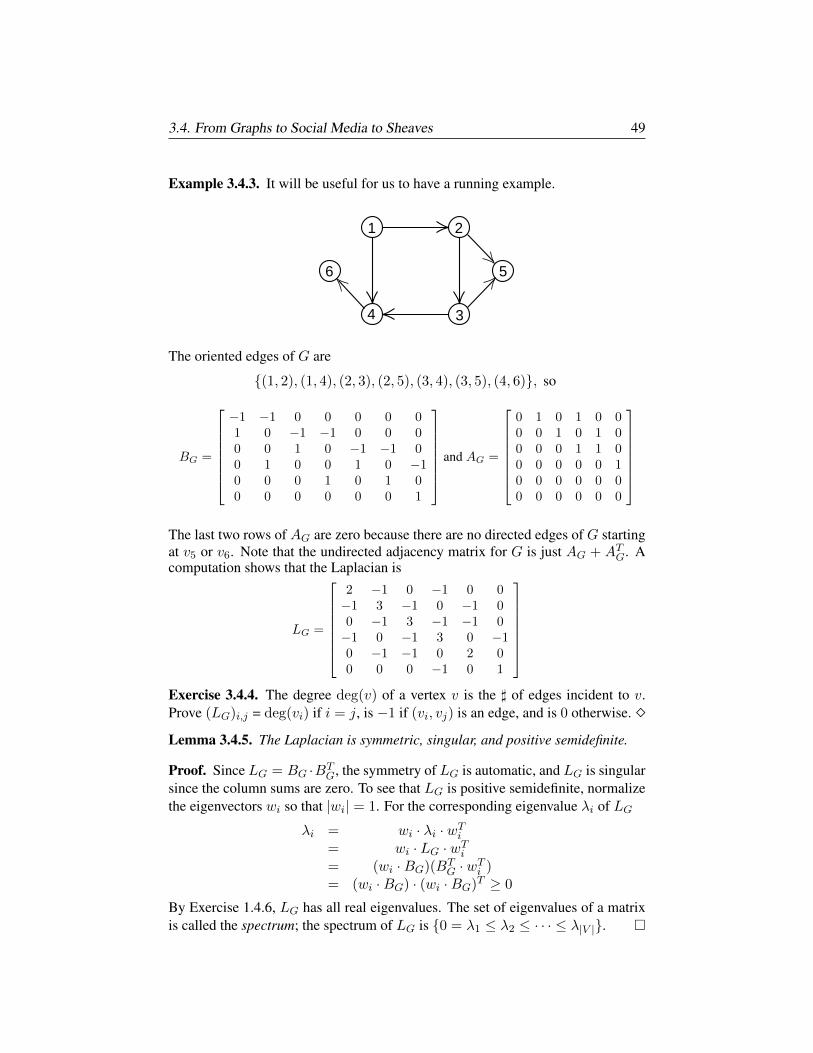
3.4. From Graphs to Social Media to Sheaves 49
Example 3.4.3. It will be useful for us to have a running example.
1 2
4 3
6 5
The oriented edges of G are
(1, 2), (1, 4), (2, 3), (2, 5), (3, 4), (3, 5), (4, 6), so
BG =
−1 −1 0 0 0 0 01 0 −1 −1 0 0 00 0 1 0 −1 −1 00 1 0 0 1 0 −10 0 0 1 0 1 00 0 0 0 0 0 1
and AG =
0 1 0 1 0 00 0 1 0 1 00 0 0 1 1 00 0 0 0 0 10 0 0 0 0 00 0 0 0 0 0
The last two rows of AG are zero because there are no directed edges of G startingat v5 or v6. Note that the undirected adjacency matrix for G is just AG + ATG. Acomputation shows that the Laplacian is
LG =
2 −1 0 −1 0 0−1 3 −1 0 −1 00 −1 3 −1 −1 0−1 0 −1 3 0 −10 −1 −1 0 2 00 0 0 −1 0 1
Exercise 3.4.4. The degree deg(v) of a vertex v is the ] of edges incident to v.Prove (LG)i,j = deg(vi) if i = j, is −1 if (vi, vj) is an edge, and is 0 otherwise. Lemma 3.4.5. The Laplacian is symmetric, singular, and positive semidefinite.
Proof. Since LG = BG ·BTG, the symmetry of LG is automatic, and LG is singular
since the column sums are zero. To see that LG is positive semidefinite, normalizethe eigenvectors wi so that |wi| = 1. For the corresponding eigenvalue λi of LG
λi = wi · λi · wTi= wi · LG · wTi= (wi ·BG)(BT
G · wTi )= (wi ·BG) · (wi ·BG)T ≥ 0
By Exercise 1.4.6, LG has all real eigenvalues. The set of eigenvalues of a matrixis called the spectrum; the spectrum of LG is 0 = λ1 ≤ λ2 ≤ · · · ≤ λ|V |.
50 3. Basics of Topology: Spaces and Sheaves
In Chapter 4, you will prove that the number of connected components of G isthe dimension of the nullspace of LG. So if G is connected, 0 < λ2; this numberis called the algebraic connectivity, and is closely related to the smallest cut of G.A cut is a partition of V into two disjoint subsets V1 t V2, and the cutset is the setof edges having one vertex in V1 and one vertex in V2. This turns out to be relatedto bottleneck distance, which appears in Chapter 7.
3.4.2. Heat diffusing on a wire graph. Now we imagine our graphG as a collec-tion of wires, with heat sources placed at the vertices. For a vertex vi ∈ G and timet, what is the temperature ui(t)? By Newton’s law of cooling, the heat flow alongan edge [vi, vj ] is proportional to the difference in temperature at the two vertices:
duidt
= −k ·∑j
(AG)ij(ui − uj),where k is the conductivity of the wire.
Now we rearrange things and consolidate
= −k · ui∑j
(AG)ij − k ·∑j
(AG)ij(−uj)
= −k · ui · deg(vi)− k ·∑j
(AG)ij(−uj)
= −k ·∑j
(LG)uj
This yields a system of first order ordinary differential equations, which we cansolve by diagonalization. To solve a system of first order ODE’s–that is, a systemof equations of the form y′i =
∑aiyi, with i ∈ 1, . . . , n–we write the system in
the form below, with A an n× n matrix:
y′ = Ay, where y = (y1, . . . , yn)T , and y′ = (y′1, . . . , y′n)T .
Now let y = Pw for an n× n matrix P , so that y′ = Pw′, and
Pw′ = y′ = Ay = APw⇒ w′ = P−1APw.
If we can find a P so that P−1AP = D is diagonal, we reduce to solving asystem of equations of the form w′i = biwi, so that wi = cie
bit. So our goal is todiagonalize A, solve for w, then back substitute via y = Pw to solve for y.
Example 3.4.6. Add the edge (1, 6) to the graph G of Example 3.4.3, and callthe new graph H (this is so we have nice eigenvalues: LG has only 2 integraleigenvalues). If we let k = 1, then−LH has eigenvalues 0,−1,−3,−3,−4,−5,so w = (c1, c2e
−t, c3e−3t, c4e
−3t, c5e−4t, c6e
−5t), with y = Pw.
−LH =
−3 1 0 1 0 11 −3 1 0 1 00 1 −3 1 1 01 0 1 −3 0 10 1 1 0 −2 01 0 0 1 0 −2
and P =
1 1 1 1 1 11 −1 1 1 −1 −11 −1 −1 0 −1 11 1 −1 0 1 −11 −2 0 −1 1 01 2 0 −1 −1 0
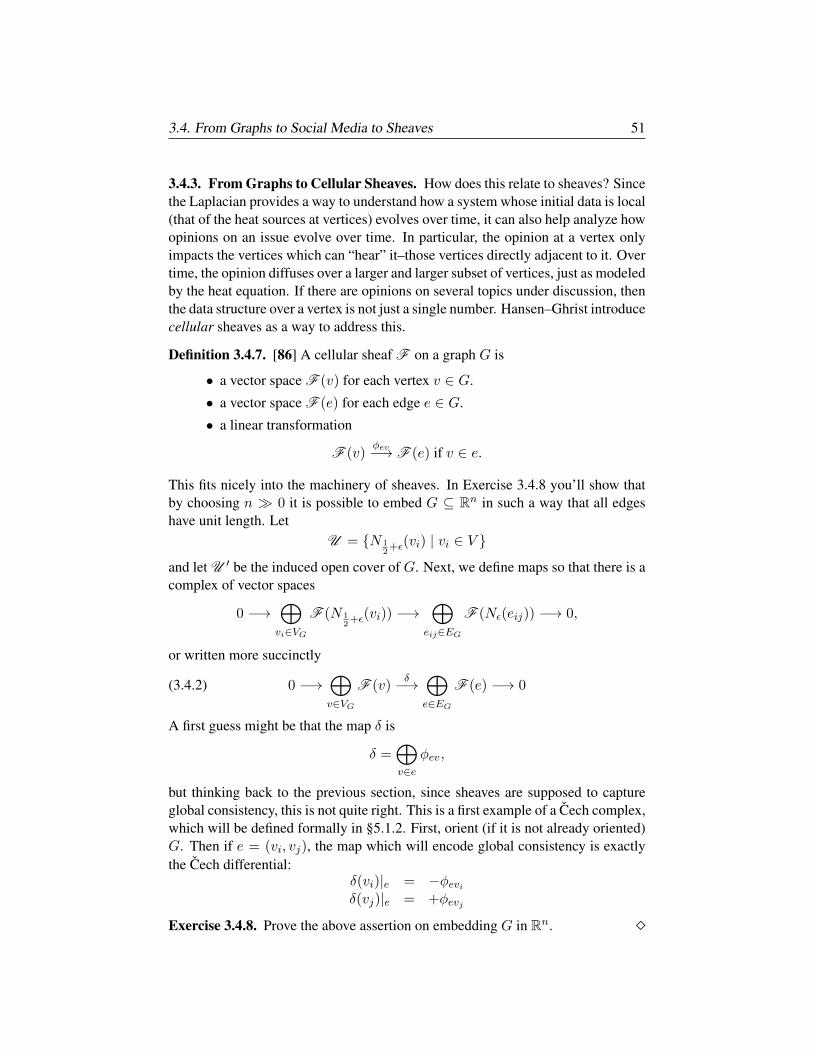
3.4. From Graphs to Social Media to Sheaves 51
3.4.3. From Graphs to Cellular Sheaves. How does this relate to sheaves? Sincethe Laplacian provides a way to understand how a system whose initial data is local(that of the heat sources at vertices) evolves over time, it can also help analyze howopinions on an issue evolve over time. In particular, the opinion at a vertex onlyimpacts the vertices which can “hear” it–those vertices directly adjacent to it. Overtime, the opinion diffuses over a larger and larger subset of vertices, just as modeledby the heat equation. If there are opinions on several topics under discussion, thenthe data structure over a vertex is not just a single number. Hansen–Ghrist introducecellular sheaves as a way to address this.
Definition 3.4.7. [86] A cellular sheaf F on a graph G is
• a vector space F (v) for each vertex v ∈ G.
• a vector space F (e) for each edge e ∈ G.
• a linear transformation
F (v)φev−→ F (e) if v ∈ e.
This fits nicely into the machinery of sheaves. In Exercise 3.4.8 you’ll show thatby choosing n 0 it is possible to embed G ⊆ Rn in such a way that all edgeshave unit length. Let
U = N 12
+ε(vi) | vi ∈ V
and let U ′ be the induced open cover of G. Next, we define maps so that there is acomplex of vector spaces
0 −→⊕vi∈VG
F (N 12
+ε(vi)) −→⊕
eij∈EG
F (Nε(eij)) −→ 0,
or written more succinctly
(3.4.2) 0 −→⊕v∈VG
F (v)δ−→⊕e∈EG
F (e) −→ 0
A first guess might be that the map δ is
δ =⊕v∈e
φev,
but thinking back to the previous section, since sheaves are supposed to captureglobal consistency, this is not quite right. This is a first example of a Cech complex,which will be defined formally in §5.1.2. First, orient (if it is not already oriented)G. Then if e = (vi, vj), the map which will encode global consistency is exactlythe Cech differential:
δ(vi)|e = −φeviδ(vj)|e = +φevj
Exercise 3.4.8. Prove the above assertion on embedding G in Rn.

52 3. Basics of Topology: Spaces and Sheaves
In Proposition 5.2.3 of Chapter 5 we prove that if
V1d1−→ V2
d2−→ V3
is a complex of inner product spaces, then
(3.4.3) V2 ' im(d1)⊕ im(dT2 )⊕ ker(L), where L = d1dT1 + dT2 d2.
In general, the homology of a complex is simply a quotient, which has no canonicalbasis. The point is that with the extra structure we have in an inner product space,there is a canonical decomposition, and
ker(d2)/im(d1) ' ker(L).
Applying this to Equation 3.4.2, we observe that the global sections of the cellularsheaf F have a representation as the kernel of the sheaf Laplacian:
H0(F ) = ker(δT · δ).
This seems very far afield from the nice concrete graph Laplacian we began with,but the exercise below shows that is not the case.
Exercise 3.4.9. Prove that if F (v) = F (e) = K, then LG = δT · δ. Hint: makesure that you make consistent choices for the ordered bases. Next, show that wecan measure how far an element c0 ∈ C0(F ) is from being in H0(F ): if we letC0(F )
π→ H0(F ) be orthogonal projection, d(c0, H0(F )) = |c0 − π(c0)|.
Example 3.4.10. Define a sheaf on the graph H of Example 3.4.6 as follows: ateach vertex, we have the vector space Vi = Q2. Vertices represent individuals, andthe values at vertex i represent opinions on the following statements:
The best animal for a pet is a dogThe best weather is cold and snowy
Suppose −1 represents ”strongly disagree” and 1 represents ”strongly agree”. Astime goes by, individuals communicate with adjacent nodes, and opinions change.After a long period of time, the system will reach equilibrium and the opinion onany issue will be the same at all vertices. What is the status of opinions after a shortperiod of time, for example, before the opinion at vertex 5 and vertex 6 (the mostdistant vertices) have reached each other? Suppose the opinions on statement 1 arey(0) = 0, 0, 0, 0,−1, 1. Note that w(0) = P−1y(0) and
P−1 =1
12
2 2 2 2 2 21 −1 −1 1 −2 22 2 −4 −4 2 22 2 2 2 −4 −42 −2 −2 2 2 −23 −3 3 −3 0 0
.
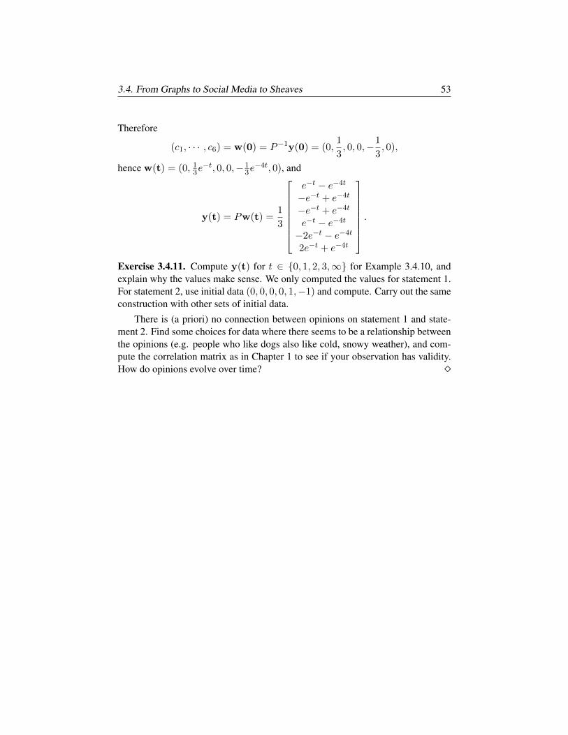
3.4. From Graphs to Social Media to Sheaves 53
Therefore
(c1, · · · , c6) = w(0) = P−1y(0) = (0,1
3, 0, 0,−1
3, 0),
hence w(t) = (0, 13e−t, 0, 0,−1
3e−4t, 0), and
y(t) = Pw(t) =1
3
e−t − e−4t
−e−t + e−4t
−e−t + e−4t
e−t − e−4t
−2e−t − e−4t
2e−t + e−4t
.
Exercise 3.4.11. Compute y(t) for t ∈ 0, 1, 2, 3,∞ for Example 3.4.10, andexplain why the values make sense. We only computed the values for statement 1.For statement 2, use initial data (0, 0, 0, 0, 1,−1) and compute. Carry out the sameconstruction with other sets of initial data.
There is (a priori) no connection between opinions on statement 1 and state-ment 2. Find some choices for data where there seems to be a relationship betweenthe opinions (e.g. people who like dogs also like cold, snowy weather), and com-pute the correlation matrix as in Chapter 1 to see if your observation has validity.How do opinions evolve over time?

Chapter 4
Homology I: SimplicialComplexes to SensorNetworks
This chapter is the fulcrum of the book, the beginning of a beautiful friendship be-tween algebra and topology. The idea is the following: small open neighborhoodsof a point on the circle S1 and a point on the line R1 are homeomorphic–an antliving in either neighborhood would be unable to distinguish between them. Butfrom a global perspective we can easily spot the difference between R1 and S1.Homology provides a way to quantify and compute the difference.
The first step is to model a topological space combinatorially. We do this withsimplicial complexes, which are a lego set for topologists. The second step is totranslate the combinatorial data of a simplicial complex into an algebraic complex,as in Equation 2.2.1 of Chapter 2. Simplicial homology is the homology of theresulting complex; we also discuss singular homology, which is based on formalcombinations of maps from a simplex into a topological space.
In §3 we introduce the basics of homological algebra, and in §4 we connectback to topology via the Mayer–Vietoris sequence, which describes how buildinga simplicial complex from constituent parts translates into algebra, and introduceRips–Vietoris and Cech complexes, which play a central role in data analysis. Thetopics covered in this chapter are:
• Simplicial Complexes, Nerve of a Cover.
• Simplicial and Singular Homology.
• Snake Lemma and Long Exact Sequence in Homology.
• Mayer–Vietoris, Rips–Vietoris and Cech complexes, Sensor Networks.
55
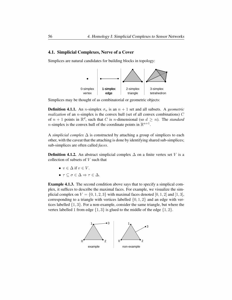
56 4. Homology I: Simplicial Complexes to Sensor Networks
4.1. Simplicial Complexes, Nerve of a Cover
Simplices are natural candidates for building blocks in topology:
0-simplexvertex
1-simplexedge
3-simplextetrahedron
1-simplexedge
2-simplextriangle
Simplices may be thought of as combinatorial or geometric objects:
Definition 4.1.1. An n-simplex σn is an n + 1 set and all subsets. A geometricrealization of an n-simplex is the convex hull (set of all convex combinations) Cof n + 1 points in Rd, such that C is n-dimensional (so d ≥ n). The standardn-simplex is the convex hull of the coordinate points in Rn+1.
A simplicial complex ∆ is constructed by attaching a group of simplices to eachother, with the caveat that the attaching is done by identifying shared sub-simplices;sub-simplices are often called faces.
Definition 4.1.2. An abstract simplicial complex ∆ on a finite vertex set V is acollection of subsets of V such that
• v ∈ ∆ if v ∈ V .
• τ ⊆ σ ∈ ∆⇒ τ ∈ ∆.
Example 4.1.3. The second condition above says that to specify a simplical com-plex, it suffices to describe the maximal faces. For example, we visualize the sim-plicial complex on V = 0, 1, 2, 3 with maximal faces denoted [0, 1, 2] and [1, 3],corresponding to a triangle with vertices labelled 0, 1, 2 and an edge with ver-tices labelled 1, 3. For a non-example, consider the same triangle, but where thevertex labelled 1 from edge 1, 3 is glued to the middle of the edge 1, 2.
example non-example
1
20
3
20
13
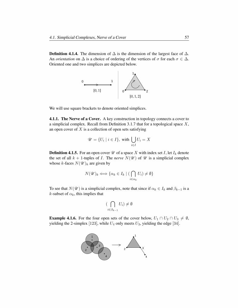
4.1. Simplicial Complexes, Nerve of a Cover 57
Definition 4.1.4. The dimension of ∆ is the dimension of the largest face of ∆.An orientation on ∆ is a choice of ordering of the vertices of σ for each σ ∈ ∆.Oriented one and two simplices are depicted below.
20
1
0 1
We will use square brackets to denote oriented simplices.
4.1.1. The Nerve of a Cover. A key construction in topology connects a cover toa simplicial complex. Recall from Definition 3.1.7 that for a topological space X ,an open cover of X is a collection of open sets satisfying
U = Ui | i ∈ I, with⋃i∈I
Ui = X
Definition 4.1.5. For an open cover U of a space X with index set I , let Ik denotethe set of all k + 1-tuples of I . The nerve N(U ) of U is a simplicial complexwhose k-faces N(U )k are given by
N(U )k ⇐⇒ αk ∈ Ik | (⋂i∈αk
Ui) 6= ∅
To see that N(U ) is a simplicial complex, note that since if αk ∈ Ik and βk−1 is ak-subset of αk, this implies that
(⋂
i∈βk−1
Ui) 6= ∅
Example 4.1.6. For the four open sets of the cover below, U1 ∩ U2 ∩ U3 6= ∅,yielding the 2-simplex [123], while U4 only meets U3, yielding the edge [34].
1
4
2 3
1
2
3
4
58 4. Homology I: Simplicial Complexes to Sensor Networks
Theorem 4.1.7. If U is a finite open cover of X , and all intersections of the opensets of U are contractible or empty, then N(U ) is homotopic to X .
Theorem 4.1.7 is called the Nerve Theorem, and follows from Theorem 9.4.5; seealso Exercise 5.1.5. In §4 of this chapter, we’ll see two standard ways to build asimplicial complex ∆ε from the space Xε appearing in the introduction; the firstway is via the nerve of a cover. The Nerve Theorem also holds for a closed coverof a CW-complex (which are defined in §5.3) by subcomplexes, see [16].
4.2. Simplicial and Singular Homology
We recall the definition of an algebraic complex from Chapter 2: a complex C isa sequence of modules and homomorphisms
C• : · · ·Mj+1dj+1−→Mj
dj−→Mj−1 · · ·
such that im(dj+1) ⊆ ker(dj); the jth homology is Hj(C ) = ker(dj)/im(dj+1).
Definition 4.2.1. Let ∆ be an oriented simplicial complex, and let R be a ring.Define Ci(∆, R) as the free R-module with basis the oriented i-simplices, modulothe relations
[v0, . . . , vn] ∼ (−1)sgn(σ)[vσ(0), . . . , vσ(n)],
where σ ∈ Sn+1 is a permutation. Any permutation σ can be written as a productof transpositions (two cycles); the sign of σ is one if the number of transpositionsis odd, and zero if the number of transpositions is even.
Example 4.2.2. For an edge, this says
[v0, v1] = −[v1, v0]
This is familiar from vector calculus: when it comes to integration∫ v1
v0
f(x)dx = −∫ v0
v1
f(x)dx
For a triangle, the orientation [v2, v1, v0] requires 3 transpositions to change to[v0, v1, v2], hence
[v2, v1, v0] = −[v0, v1, v2]
Definition 4.2.3. Let ∂ be the map from Ci(∆, R) to Ci−1(∆, R) defined by
∂([vj0 , . . . , vji ]) =
i∑k=0
(−1)k[vj0 , . . . , vjk , . . . , vji ], where v means omit v.
The map ∂ is called the boundary map; it sends an i-simplex to a signed sum of itsi− 1 faces. Applying ∂2 to a basis element shows ∂2 = 0, so the Ci form a chaincomplex C . Simplicial homology Hi(∆, R) is the homology of C .
4.2. Simplicial and Singular Homology 59
Example 4.2.4. If R is a field, then the Ci form a complex of vector spaces Vi.
V : 0 −→ Vn −→ Vn−1 −→ · · · −→ V0 −→ 0.
An induction shows thatn∑i=0
(−1)i dimVi =n∑i=0
(−1)i dimHi(V ).
The alternating sum χ(V ) above is known as the Euler characteristic.
Example 4.2.5. We return to our pair of ants, one living on S1 and one on R1. LetK be a field, and model S1 and (a portion of) R1 with oriented simplicial complexes∆1 and ∆2 having maximal faces
∆1 = [0, 1], [1, 2], [2, 0] and ∆2 = [0, 1], [1, 2], [2, 3]Let C1(∆i,K) have the ordered bases above, and order the basis of C0(∆1,K) as[0], [1], [2]. With respect to these bases, the only nonzero differential is ∂1:
C•(∆1,K) = 0 −→ K3
∂1=
−1 0 11 −1 00 1 −1
// K3 −→ 0
and we compute that H1(∆1) = ker(∂1) = [1, 1, 1]T . On the other hand, for ∆2,using [0], [1], [2], [3] as the ordered basis for C0(∆2), the complex is
C•(∆2,K) = 0 −→ K3
∂1=
−1 0 01 −1 00 1 −10 0 1
// K4 −→ 0
and we compute that H1(∆2) = 0. So H1 distinguishes between ∆1 and ∆2.
Exercise 4.2.6. The example above illustrates the key point about homology: Fork ≥ 1, Hk measures k-dimensional holes. Draw a picture and compute homologywhen ∆ has oriented simplices [0, 1], [1, 2], [2, 0], [2, 3], [0, 3] Exercise 4.2.7. If we augment C by adding in the empty face so C−1(∆, R) = R,the result is reduced homology Hi(∆, R). Show Hi(∆, R) = Hi(∆, R) for i ≥ 1,and H0(∆, R) = 0 iff ∆ is connected. Simplicial homology is a topological invariant, which can be proved by takingcommon refinements of two different triangulations. For an infinite simplicialcomplex, we define elements of Ci(∆, R) as functions c from the i-simplices toR which are zero except on finitely many simplices, such that if τ and τ ′ are thesame as unoriented simplices and τ = σ(τ ′) then c(τ) = sgn(σ)c(τ ′). This will beuseful in §4.2.1, where we define singular homology, for which topological invari-ance is automatic. The downside is that singular homology is difficult to compute.
60 4. Homology I: Simplicial Complexes to Sensor Networks
Example 4.2.8. We compute the simplicial homology of the sphere S2, using twodifferent triangulations. Let ∆1 be the simplicial complex defined by the boundaryof a tetrahedron, having maximal faces [1, 2, 3], [1, 2, 4], [1, 3, 4], [2, 3, 4], and let∆2 be the simplicial complex consisting of two hollow tetrahedra, glued along acommon triangular face, with the glued face subsequently removed; ∆2 has maxi-mal faces [1, 2, 4], [1, 3, 4], [2, 3, 4], [1, 2, 5], [1, 3, 5], [2, 3, 5].
3
2
4
1
5
3
21
4
With oriented, ordered basis forC2(∆1, R) as above, oriented basis forC1(∆1, R) =[1, 2], [1, 3], [1, 4], [2, 3], [2, 4], [3, 4], and basis forC0(∆1, R) = [1], [2], [3], [4],the complex C•(∆1, R) is given by
0 // R4 ∂2 // R6 ∂1 // R4 // 0
with
∂2 =
1 1 0 0−1 0 1 00 −1 −1 01 0 0 10 1 0 −10 0 1 1
and ker(∂2) = [1,−1, 1,−1]T
and
∂1 =
−1 −1 −1 0 0 01 0 0 −1 −1 00 1 0 1 0 −10 0 1 0 1 1
We compute ker(∂1) = im(∂2), and im(∂1) ' R3 ⊆ R4 = ker(∂0), hence
H2(∆1, R) ' R1
H1(∆1, R) ' 0H0(∆1, R) ' R1
Exercise 4.2.9. Compute Hi(∆2, R). You should obtain the same values for ho-mology as above: H1(∆2, R) vanishes, and H2(∆2, R) ' R ' H0(∆2, R). We’llsee in Chapter 5 that this symmetry is a consequence of Poincare duality. The simplest possible model for S2 would consist of two triangles, glued togetheralong the 3 common edges. The definition of CW complexes in Chapter 5 willallow this, and in fact permit an even simpler model for S2.
4.2. Simplicial and Singular Homology 61
4.2.1. Singular homology. In singular homology, the objects of study are maps toa topological spaceX . A singular n-simplex is a continuous map from the standardn-simplex ∆n to X . The free abelian group on the singular n-simplices on X isthe singular n-chains Sn(X). If σ ∈ Sn(X), then restricting σ to an n − 1 faceof ∆n yields (after an appropriate change of coordinates) an element of Sn−1(X),and we can build a chain complex just as we did with simplicial homology:
Definition 4.2.10. Let ri be the map that changes coordinates from the basis vec-tors e1, . . . , ei, . . . , en+1 to the basis vectors e1, . . . , en. For
f ∈ Sn(X), let fi be the restriction of f to the ith face of ∆n,
and define a complex S : · · · −→ Sn(X)∂−→ Sn−1(X) −→ · · · via
∂(f) =n+1∑i=1
(−1)irifi.
The ri are needed to shift the domain of definition for the restricted map fi to thestandard n − 1 simplex, which is the source for the n − 1 chains. A check showsthat ∂2 = 0, and singular homology is defined as the homology of the complex S .
Theorem 4.2.11. If X and Y are homotopic, then Hi(X) ' Hi(Y ).
Proof. (Sketch) If f is map between topological spaces or simplicial complexes,it gives rise to an induced map f∗ on homology. A pair of maps f∗, g∗ betweenchain complexes are homotopic if Definition 4.3.7 holds. Theorem 4.3.8 showshomotopic maps of chain complexes induce the same map on homology. The resultfollows by Exercise 7.4.6, which connects topological & algebraic homotopy.
We noted earlier that it is not obvious that simplicial homology is a topologicalinvariant. In fact, there is an isomorphism between the singular and simplicialhomology of a space X , and we close with a sketch of the proof.
Theorem 4.2.12. For a topological space X which can be triangulated, there isan isomorphism from the simplicial homology ofX to the singular homology ofX .
Proof. (Sketch) Let K be a triangulation of X , so Si(X) = Si(K). Then the map
φ : Ci(K,R) −→ Si(X)
defined by sending an i-simplex σ ∈ Ki to the map taking the standard i-simplex toσ commutes with the differentials of C• and S•, so by Lemma 4.3.4 of this chapterthere is an induced map
φ∗ : Hi(K,R) −→ Hi(X)
To show the map is an isomorphism, first prove it when K is a finite simplicialcomplex, by inducting on the number of simplices. When K is infinite, a class insingular homology is supported on a compact subset C. Then one shows that thereis a finite subcomplex of K containing C, reducing back to the finite case.
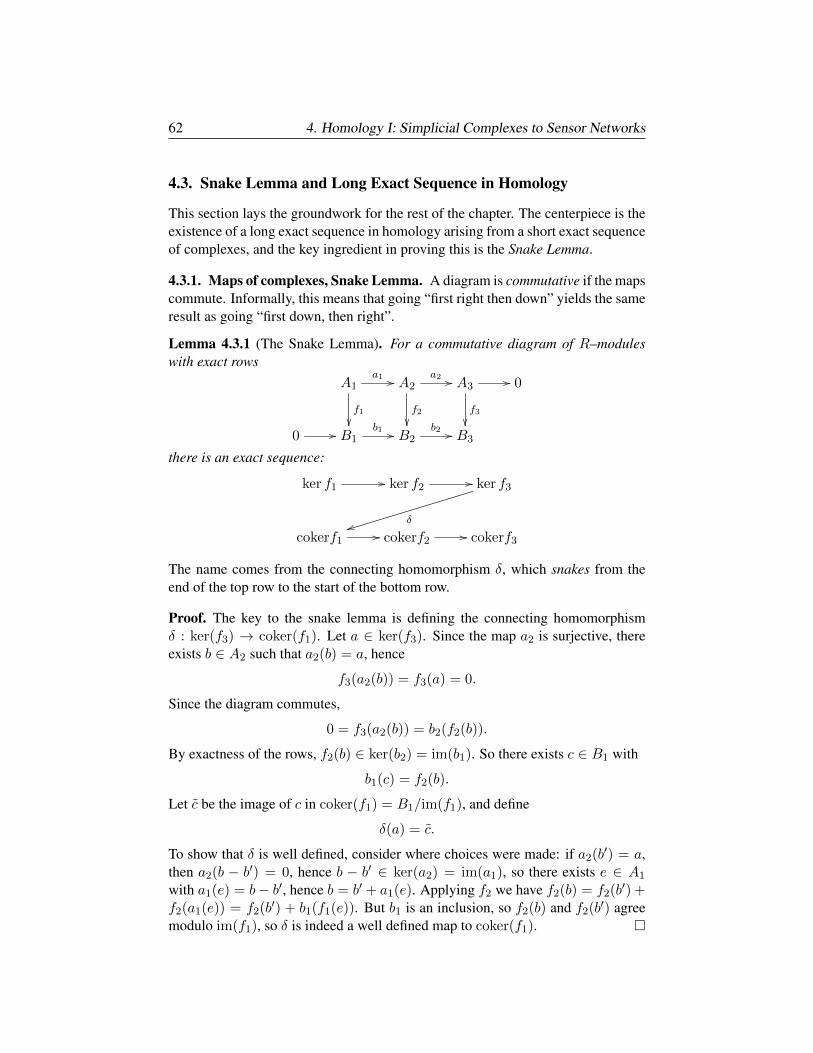
62 4. Homology I: Simplicial Complexes to Sensor Networks
4.3. Snake Lemma and Long Exact Sequence in Homology
This section lays the groundwork for the rest of the chapter. The centerpiece is theexistence of a long exact sequence in homology arising from a short exact sequenceof complexes, and the key ingredient in proving this is the Snake Lemma.
4.3.1. Maps of complexes, Snake Lemma. A diagram is commutative if the mapscommute. Informally, this means that going “first right then down” yields the sameresult as going “first down, then right”.
Lemma 4.3.1 (The Snake Lemma). For a commutative diagram of R–moduleswith exact rows
A1a1 //
f1
A2a2 //
f2
A3//
f3
0
0 // B1b1 // B2
b2 // B3
there is an exact sequence:
ker f1// ker f2
// ker f3
δttcokerf1
// cokerf2// cokerf3
The name comes from the connecting homomorphism δ, which snakes from theend of the top row to the start of the bottom row.
Proof. The key to the snake lemma is defining the connecting homomorphismδ : ker(f3) → coker(f1). Let a ∈ ker(f3). Since the map a2 is surjective, thereexists b ∈ A2 such that a2(b) = a, hence
f3(a2(b)) = f3(a) = 0.
Since the diagram commutes,
0 = f3(a2(b)) = b2(f2(b)).
By exactness of the rows, f2(b) ∈ ker(b2) = im(b1). So there exists c ∈ B1 with
b1(c) = f2(b).
Let c be the image of c in coker(f1) = B1/im(f1), and define
δ(a) = c.
To show that δ is well defined, consider where choices were made: if a2(b′) = a,then a2(b − b′) = 0, hence b − b′ ∈ ker(a2) = im(a1), so there exists e ∈ A1
with a1(e) = b− b′, hence b = b′ + a1(e). Applying f2 we have f2(b) = f2(b′) +f2(a1(e)) = f2(b′) + b1(f1(e)). But b1 is an inclusion, so f2(b) and f2(b′) agreemodulo im(f1), so δ is indeed a well defined map to coker(f1).
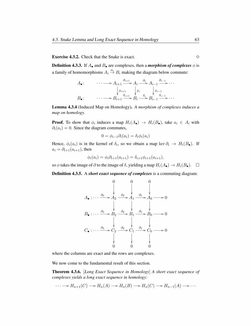
4.3. Snake Lemma and Long Exact Sequence in Homology 63
Exercise 4.3.2. Check that the Snake is exact. Definition 4.3.3. If A• and B• are complexes, then a morphism of complexes φ is
a family of homomorphisms Aiφi→ Bi making the diagram below commute:
A• : · · · // Ai+1∂i+1 //
φi+1
Ai∂i //
φi
Ai−1∂i−1 //
φi−1
· · ·
B• : · · · // Bi+1δi+1 // Bi
δi // Bi−1δi−1 // · · ·
Lemma 4.3.4 (Induced Map on Homology). A morphism of complexes induces amap on homology.
Proof. To show that φi induces a map Hi(A•) → Hi(B•), take ai ∈ Ai with∂i(ai) = 0. Since the diagram commutes,
0 = φi−1∂i(ai) = δiφi(ai)
Hence, φi(ai) is in the kernel of δi, so we obtain a map ker ∂i → Hi(B•). Ifai = ∂i+1(ai+1), then
φi(ai) = φi∂i+1(ai+1) = δi+1φi+1(ai+1),
so φ takes the image of ∂ to the image of δ, yielding a mapHi(A•)→ Hi(B•).
Definition 4.3.5. A short exact sequence of complexes is a commuting diagram:
0
0
0
A• : · · · ∂3 // A2
∂2 //
A1∂1 //
A0//
0
B• : · · · ∂3 // B2∂2 //
B1∂1 //
B0//
0
C• : · · · ∂3 // C2∂2 //
C1∂1 //
C0//
0
0 0 0
where the columns are exact and the rows are complexes.
We now come to the fundamental result of this section.
Theorem 4.3.6. [Long Exact Sequence in Homology] A short exact sequence ofcomplexes yields a long exact sequence in homology:
· · · // Hn+1(C) // Hn(A) // Hn(B) // Hn(C) // Hn−1(A) // · · ·
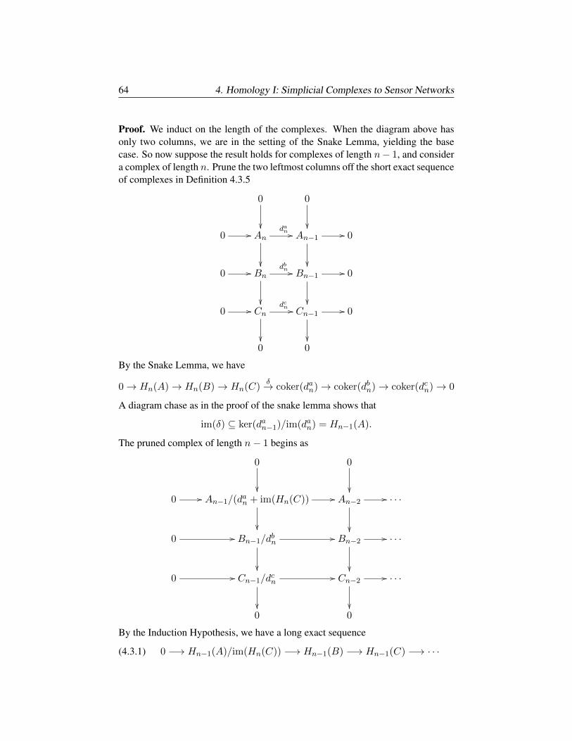
64 4. Homology I: Simplicial Complexes to Sensor Networks
Proof. We induct on the length of the complexes. When the diagram above hasonly two columns, we are in the setting of the Snake Lemma, yielding the basecase. So now suppose the result holds for complexes of length n− 1, and considera complex of length n. Prune the two leftmost columns off the short exact sequenceof complexes in Definition 4.3.5
0
0
0 // An
dan //
An−1//
0
0 // Bndbn //
Bn−1//
0
0 // Cndcn //
Cn−1//
0
0 0
By the Snake Lemma, we have
0→ Hn(A)→ Hn(B)→ Hn(C)δ→ coker(dan)→ coker(dbn)→ coker(dcn)→ 0
A diagram chase as in the proof of the snake lemma shows that
im(δ) ⊆ ker(dan−1)/im(dan) = Hn−1(A).
The pruned complex of length n− 1 begins as
0
0
0 // An−1/(d
an + im(Hn(C)) //
An−2//
· · ·
0 // Bn−1/dbn
//
Bn−2//
· · ·
0 // Cn−1/dcn
//
Cn−2//
· · ·
0 0
By the Induction Hypothesis, we have a long exact sequence
(4.3.1) 0 −→ Hn−1(A)/im(Hn(C)) −→ Hn−1(B) −→ Hn−1(C) −→ · · ·
4.4. Mayer–Vietoris, Rips and Cech complex, Sensor Networks 65
Since im(δ) ⊆ Hn−1(A), we also have an exact sequence
(4.3.2) · · · → Hn(C)δ−→ Hn−1(A)→ Hn−1(A)/Hn(C)→ 0.
To conclude, splice the surjection of Equation 4.3.2
Hn−1(A)→ Hn−1(A)/Hn(C)→ 0
with the inclusion of Equation 4.3.1
0→ Hn−1(A)/Hn(C)→ Hn−1(B),
to obtain a map Hn−1(A)→ Hn−1(B), which completes the induction.
4.3.2. Chain Homotopy. When do two morphisms of complexes induce the samemap on homology?
Definition 4.3.7. IfA andB are complexes, and α, β are morphisms of complexes,then α and β are homotopic if there exists a family of homomorphismsAi
γi→ Bi+1
such that for all i, αi − βi = δi+1γi + γi−1∂i; a diagram illustrating this appearsin Exercise 7.4.6. Notice that γ need not commute with ∂ and δ.
Theorem 4.3.8. Homotopic maps induce the same map on homology.
Proof. It suffices to show that if αi = δi+1γi+γi−1∂i then α induces the zero mapon homology. But if ai ∈ Hi(A), then since ∂i(ai) = 0,
αi(ai) = δi+1γi(ai) + γi−1∂i(ai) = δi+1γi(ai) ∈ im(δ),
so αi(ai) = 0 in Hi(B).
4.4. Mayer–Vietoris, Rips and Cech complex, Sensor Networks
As we noted at the beginning of the chapter, homological algebra grew out oftopology, and we illustrate this now.
4.4.1. Mayer–Vietoris sequence. A central idea in mathematics is to study anobject by splitting it into simpler component parts. The Mayer–Vietoris sequenceprovides a way to do this in the topological setting. Basically, Mayer–Vietoris is a“divide and conquer” strategy. Given a topological space or simplicial complex Z,if we write
Z = X ∪ Ythen there will be relations between X , Y , Z and the intersection X ∩ Y .
Theorem 4.4.1 (Mayer–Vietoris). Let X and Y be simplicial complexes, and letZ = X ∪ Y . Then there is a short exact sequence of complexes
0 −→ C•(X ∩ Y ) −→ C•(X)⊕ C•(Y ) −→ C•(X ∪ Y ) −→ 0,
yielding a long exact sequence in homology.
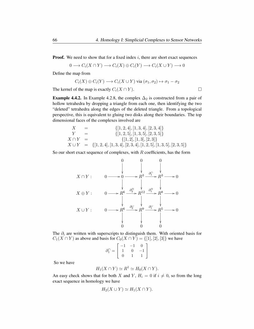
66 4. Homology I: Simplicial Complexes to Sensor Networks
Proof. We need to show that for a fixed index i, there are short exact sequences
0 −→ Ci(X ∩ Y ) −→ Ci(X)⊕ Ci(Y ) −→ Ci(X ∪ Y ) −→ 0
Define the map from
Ci(X)⊕ Ci(Y ) −→ Ci(X ∪ Y ) via (σ1, σ2) 7→ σ1 − σ2
The kernel of the map is exactly Ci(X ∩ Y ).
Example 4.4.2. In Example 4.2.8, the complex ∆2 is constructed from a pair ofhollow tetrahedra by dropping a triangle from each one, then identifying the two“deleted” tetrahedra along the edges of the deleted triangle. From a topologicalperspective, this is equivalent to gluing two disks along their boundaries. The topdimensional faces of the complexes involved are
X = [1, 2, 4], [1, 3, 4], [2, 3, 4]Y = [1, 2, 5], [1, 3, 5], [2, 3, 5]
X ∩ Y = [1, 2], [1, 3], [2, 3]X ∪ Y = [1, 2, 4], [1, 3, 4], [2, 3, 4], [1, 2, 5], [1, 3, 5], [2, 3, 5]
So our short exact sequence of complexes, with R coefficients, has the form
0
0
0
X ∩ Y : 0 // 0 //
R3∂∩1 //
R3 //
0
X ⊕ Y : 0 // R6∂⊕2 //
R12∂⊕1 //
R8 //
0
X ∪ Y : 0 // R6∂∪2 //
R9∂∪1 //
R5 //
0
0 0 0
The ∂i are written with superscripts to distinguish them. With oriented basis forC1(X ∩ Y ) as above and basis for C0(X ∩ Y ) = [1], [2], [3] we have
∂∩1 =
−1 −1 01 0 −10 1 1
So we have
H1(X ∩ Y ) ' R1 ' H0(X ∩ Y ).
An easy check shows that for both X and Y , Hi = 0 if i 6= 0, so from the longexact sequence in homology we have
H2(X ∪ Y ) ' H1(X ∩ Y ).
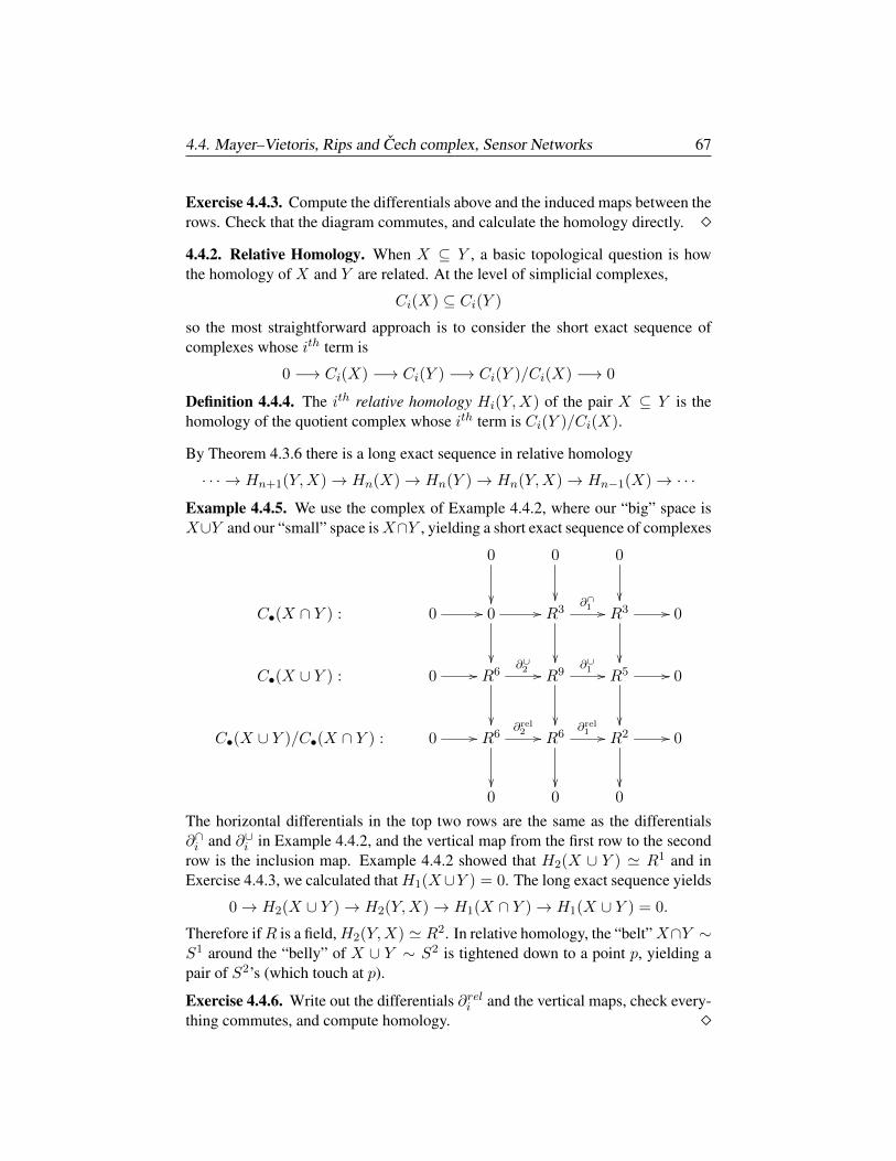
4.4. Mayer–Vietoris, Rips and Cech complex, Sensor Networks 67
Exercise 4.4.3. Compute the differentials above and the induced maps between therows. Check that the diagram commutes, and calculate the homology directly. 4.4.2. Relative Homology. When X ⊆ Y , a basic topological question is howthe homology of X and Y are related. At the level of simplicial complexes,
Ci(X) ⊆ Ci(Y )
so the most straightforward approach is to consider the short exact sequence ofcomplexes whose ith term is
0 −→ Ci(X) −→ Ci(Y ) −→ Ci(Y )/Ci(X) −→ 0
Definition 4.4.4. The ith relative homology Hi(Y,X) of the pair X ⊆ Y is thehomology of the quotient complex whose ith term is Ci(Y )/Ci(X).
By Theorem 4.3.6 there is a long exact sequence in relative homology
· · · → Hn+1(Y,X)→ Hn(X)→ Hn(Y )→ Hn(Y,X)→ Hn−1(X)→ · · ·
Example 4.4.5. We use the complex of Example 4.4.2, where our “big” space isX∪Y and our “small” space isX∩Y , yielding a short exact sequence of complexes
0
0
0
C•(X ∩ Y ) : 0 // 0 //
R3∂∩1 //
R3 //
0
C•(X ∪ Y ) : 0 // R6∂∪2 //
R9∂∪1 //
R5 //
0
C•(X ∪ Y )/C•(X ∩ Y ) : 0 // R6∂rel
2 //
R6∂rel
1 //
R2 //
0
0 0 0
The horizontal differentials in the top two rows are the same as the differentials∂∩i and ∂∪i in Example 4.4.2, and the vertical map from the first row to the secondrow is the inclusion map. Example 4.4.2 showed that H2(X ∪ Y ) ' R1 and inExercise 4.4.3, we calculated thatH1(X∪Y ) = 0. The long exact sequence yields
0→ H2(X ∪ Y )→ H2(Y,X)→ H1(X ∩ Y )→ H1(X ∪ Y ) = 0.
Therefore ifR is a field,H2(Y,X) ' R2. In relative homology, the “belt”X∩Y ∼S1 around the “belly” of X ∪ Y ∼ S2 is tightened down to a point p, yielding apair of S2’s (which touch at p).
Exercise 4.4.6. Write out the differentials ∂reli and the vertical maps, check every-thing commutes, and compute homology.
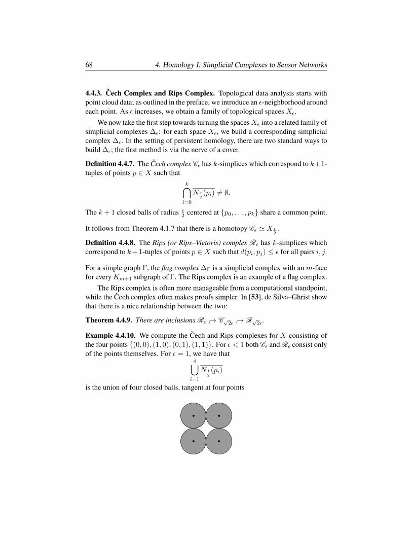
68 4. Homology I: Simplicial Complexes to Sensor Networks
4.4.3. Cech Complex and Rips Complex. Topological data analysis starts withpoint cloud data; as outlined in the preface, we introduce an ε-neighborhood aroundeach point. As ε increases, we obtain a family of topological spaces Xε.
We now take the first step towards turning the spacesXε into a related family ofsimplicial complexes ∆ε: for each space Xε, we build a corresponding simplicialcomplex ∆ε. In the setting of persistent homology, there are two standard ways tobuild ∆ε; the first method is via the nerve of a cover.
Definition 4.4.7. The Cech complex Cε has k-simplices which correspond to k+1-tuples of points p ∈ X such that
k⋂i=0
N ε2(pi) 6= ∅.
The k+ 1 closed balls of radius ε2 centered at p0, . . . , pk share a common point.
It follows from Theorem 4.1.7 that there is a homotopy Cε ' X ε2.
Definition 4.4.8. The Rips (or Rips–Vietoris) complex Rε has k-simplices whichcorrespond to k+1-tuples of points p ∈ X such that d(pi, pj) ≤ ε for all pairs i, j.
For a simple graph Γ, the flag complex ∆Γ is a simplicial complex with an m-facefor everyKm+1 subgraph of Γ. The Rips complex is an example of a flag complex.
The Rips complex is often more manageable from a computational standpoint,while the Cech complex often makes proofs simpler. In [53], de Silva–Ghrist showthat there is a nice relationship between the two:
Theorem 4.4.9. There are inclusions Rε → C√2ε → R√2ε.
Example 4.4.10. We compute the Cech and Rips complexes for X consisting ofthe four points (0, 0), (1, 0), (0, 1), (1, 1). For ε < 1 both Cε and Rε consist onlyof the points themselves. For ε = 1, we have that
4⋃i=1
N 12(pi)
is the union of four closed balls, tangent at four points

4.4. Mayer–Vietoris, Rips and Cech complex, Sensor Networks 69
Hence C1 and R1 are both (hollow) squares, as below
They remain hollow squares until ε =√
2, when all four balls meet at a commonpoint. Hence C√2 and R√2 are solid tetrahedra.
On the other hand, if X consists of the vertices of an equilateral triangle with sidesof length one, C 1
2is a hollow triangle, whereas R 1
2is a solid triangle.
Exercise 4.4.11. Let Xn consist of vertices p1, . . . , pn of a symmetric n-gon,with d(0, pi) = 1. Carry out the computation of Example 4.4.10 for Xn. We close with an application of de Silva–Ghrist [52] of homological algebra to thestudy of sensor networks.
Example 4.4.12. Suppose D ⊂ R2 is a fenced in region in the plane (hence com-pact and connected), with the fence ∂D consisting of a finite number of line seg-ments:
The region is called D because it contains a trove of diamonds. To prevent theft,the owner has deployed a sensor network. As a first step, at each vertex on ∂D,there is a fixed sensor; so we have coverage as depicted in the following diagram:
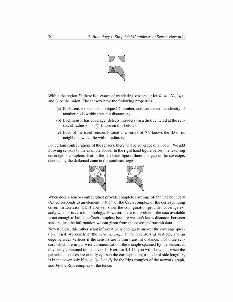
70 4. Homology I: Simplicial Complexes to Sensor Networks
Within the region D, there is a swarm of wandering sensors si; let U = Nrb(si)and U be the union. The sensors have the following properties
(a) Each sensor transmits a unique ID number, and can detect the identity ofanother node within transmit distance rb.
(b) Each sensor has coverage (detects intruders) in a disk centered at the sen-sor, of radius rc = rb√
3(more on this below).
(c) Each of the fixed sensors located at a vertex of ∂D knows the ID of itsneighbors, which lie within radius rb.
For certain configurations of the sensors, there will be coverage of all ofD. We add3 roving sensors to the example above. In the right hand figure below, the resultingcoverage is complete. But in the left hand figure, there is a gap in the coverage,denoted by the darkened zone in the southeast region.
22
1 13 3
When does a sensor configuration provide complete coverage of D? The boundary∂D corresponds to an element γ ∈ C1 of the Cech complex of the correspondingcover. In Exercise 4.4.14 you will show the configuration provides coverage ex-actly when γ is zero in homology. However, there is a problem: the data availableis not enough to build the Cech complex, because we don’t know distances betweensensors, just the information we can glean from the coverage/transmit data.
Nevertheless, this rather scant information is enough to answer the coverage ques-tion. First, we construct the network graph Γ, with sensors as vertices, and anedge between vertices if the sensors are within transmit distance. For three sen-sors which are in pairwise communication, the triangle spanned by the sensors isobviously contained in the cover. In Exercise 4.4.15, you will show that when thepairwise distances are exactly rb, then the corresponding triangle of side length rbis in the cover only if rc ≥ rb√
3. Let RΓ be the Rips complex of the network graph,
and FΓ the Rips complex of the fence.
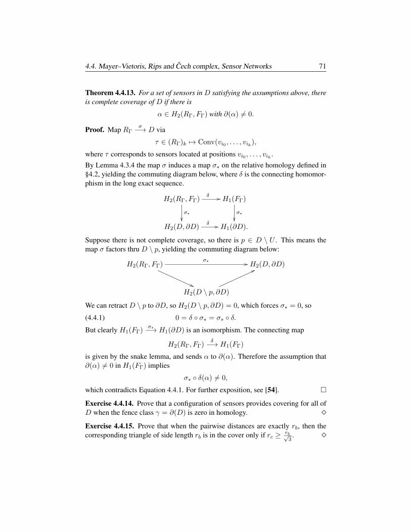
4.4. Mayer–Vietoris, Rips and Cech complex, Sensor Networks 71
Theorem 4.4.13. For a set of sensors in D satisfying the assumptions above, thereis complete coverage of D if there is
α ∈ H2(RΓ, FΓ) with ∂(α) 6= 0.
Proof. Map RΓσ−→ D via
τ ∈ (RΓ)k 7→ Conv(vi0 , . . . , vik),
where τ corresponds to sensors located at positions vi0 , . . . , vik .
By Lemma 4.3.4 the map σ induces a map σ∗ on the relative homology defined in§4.2, yielding the commuting diagram below, where δ is the connecting homomor-phism in the long exact sequence.
H2(RΓ, FΓ)δ //
σ∗
H1(FΓ)
σ∗
H2(D, ∂D)δ // H1(∂D).
Suppose there is not complete coverage, so there is p ∈ D \ U . This means themap σ factors thru D \ p, yielding the commuting diagram below:
H2(RΓ, FΓ)σ∗ //
((
H2(D, ∂D)
H2(D \ p, ∂D)
66
We can retract D \ p to ∂D, so H2(D \ p, ∂D) = 0, which forces σ∗ = 0, so
(4.4.1) 0 = δ σ∗ = σ∗ δ.But clearly H1(FΓ)
σ∗−→ H1(∂D) is an isomorphism. The connecting map
H2(RΓ, FΓ)δ−→ H1(FΓ)
is given by the snake lemma, and sends α to ∂(α). Therefore the assumption that∂(α) 6= 0 in H1(FΓ) implies
σ∗ δ(α) 6= 0,
which contradicts Equation 4.4.1. For further exposition, see [54].
Exercise 4.4.14. Prove that a configuration of sensors provides covering for all ofD when the fence class γ = ∂(D) is zero in homology. Exercise 4.4.15. Prove that when the pairwise distances are exactly rb, then thecorresponding triangle of side length rb is in the cover only if rc ≥ rb√
3.

Chapter 5
Homology II: Cohomologyto Ranking Problems
In this chapter we introduce cohomology; the constructions have roots in topologyand geometry, and as such, can come with extra structure. We begin in §1 withSimplicial, Cech, and de Rham cohomology; a first difference from homology isthat simplicial cohomology has a ring structure.
Building on de Rham cohomology, §2 begins with an overview of Hodge the-ory, which is a central (and technical) area of algebraic geometry. This is to setthe stage to describe work of Jiang–Lim–Yao–Yuan in [94] which applies Hodgetheory to ranking–specifically, the Netflix Problem, where the goal is to produce acoherent ranking from partial and inconsistent survey results, such as viewer rank-ing of movies. In particular, some rankings may involve loops: a > b > c > a.We revisit the Laplacian (Chapter 3) and describe the Hodge decomposition in asetting which only involves linear algebra.
In §3, we introduce CW complexes and cellular homology; the building blocksare cells and allow more flexibility than simplicial complexes in construction ofspaces. In §4 we tackle duality, focusing on the theories of Poincare and Alexan-der. Poincare duality is like the Tai Chi symbol–the Yin and Yang are symmetricmirrors; see [45] for use in TDA. Alexander duality is like a black and white image:knowing one color tells us the other. TDA applications appear in [1] and [82].
• Cohomology: Simplicial, Cech, de Rham theories.
• Ranking and Hodge Theory.
• CW Complexes and Cellular Homology.
• Poincare and Alexander Duality: Sensor Networks revisited.
73
74 5. Homology II: Cohomology to Ranking Problems
5.1. Cohomology: Simplicial, Cech, de Rham theories
For a complex
C : 0 −→ C0 d0
−→ C1 d1
−→ · · ·we have im(di) ⊆ ker(di+1), and the cohomology of C is defined as
H i(C ) = H i(
0 −→ C0 d0
−→ C1 d1
−→ · · ·)
So cohomology is homology with increasing indices. However, in a number ofcommon situations, there is a multiplicative structure on the set of Ci. This resultsin a multiplicative structure on cohomology, yielding a ring H∗(C ) =
⊕iH
i(C ).
5.1.1. Simplicial Cohomology. For a simplicial complex ∆ and coefficient ringR, we have the complex of R-modules
C• = · · · −→ Ci+1(∆, R)di+1−→ Ci(∆, R)
di−→ Ci−1(∆, R) −→ · · ·Applying HomR(•, R) and defining Ci(∆, R) = HomR(Ci(∆), R) yields
C • = · · · ←− Ci+1(∆, R)di←− Ci(∆, R)
di−1
←− Ci−1(∆, R)←− · · ·Elements of Ci are called i-chains, and elements of Ci are called i-cochains.
Definition 5.1.1. The multiplicative structure (called cup product) on simplicialcohomology is induced by a map on the cochains:
Ci(∆)× Cj(∆)∪−→ Ci+j(∆).
To define such a map we must define an action of a pair (ci, cj) ∈ Ci(∆)×Cj(∆)on an element of Ci+j(∆): if [v0, . . . vi+j ] = σ ∈ Ci+j(∆), then
(ci, cj)[v0, . . . vi+j ] = ci[v0, . . . , vi] · cj [vi, . . . , vi+j ],where the last · is multiplication in the ring R.
Exercise 5.1.2. Compute the simplicial cohomology rings for the complexesX∩Yand X ∪ Y of Example 4.4.2, with coefficients in a field K. Topologically,
X ∩ Y ∼ S1 and X ∪ Y ∼ S2,
so you should find H1(X ∪ Y ) = 0 and
H0(X ∩ Y ) ' K ' H1(X ∩ Y ) and H0(X ∪ Y ) ' K ' H2(X ∪ Y ).
The interesting part of the exercise is determining the multiplicative structure. Exercise 5.1.3. For the ambitious: consult a book on algebraic topology and finda triangulation of the torus T 2 (the surface of a donut). Show the cohomologyring with K coefficients is K[x, y]/〈x2, y2〉. Now do the same thing for the realprojective plane RP2, first with K = Q and then with K = Z/2 coefficients. Youshould get different answers; in particular the choice of field matters. This stemsfrom the fact that the real projective plane is not orientable.
5.1. Cohomology: Simplicial, Cech, de Rham theories 75
5.1.2. Cech Cohomology. For a sheaf F , Cech cohomology H i(F ) is constructedso that the global sections of F defined in §3 of Chapter 3 are given by the zerothcohomology. Let U = Ui be an open cover of X . If U consists of a finitenumber of open sets, then the ith module C i in the Cech complex is simply
Ci(F ,U ) =⊕
j0<...<ji
F (Uj0 ∩ · · · ∩ Uji).
In general a cover need not be finite; in this case it is convenient to think of anelement of C i as an operator ci which assigns to each (i+ 1)-tuple (j0, . . . , ji) anelement of F (Uj0 ∩ · · · ∩ Uji). We build a complex C • via:
C i =∏
j0<...<ji
F (Uj0 ∩ · · · ∩ Uji)di−→ C i+1 =
∏j0<...<ji+1
F (Uj0 ∩ · · · ∩ Uji+1),
where di(ci) is defined by how it operates on (i+ 2)-tuples, which is:
di(ci)(j0, . . . , ji+1) =
i+1∑k=0
(−1)kci(j0, . . . , jk, . . . , ji+1)|F (Uj0∩···∩Uji+1).
Definition 5.1.4. The ith Cech cohomology of F and U is H i(U ,F ) = H i(C •).
Exercise 5.1.5. The constant sheaf on a spaceX is defined by giving Z the discretetopology, and defining Z(U) as the space of continuous functions from U to Z.
(a) Is it true that Z(U) ' Z for any open set U? If not, what additionalassumption on U would make this true?
(b) Compute the Cech cohomology of the constant sheaf Z on S2 using thecover of the open top hemisphere, and the two open bottom “quarter-spheres” (all opens slightly enlarged so that they overlap) and see whatyou get. Your chain complex should start with these three opens (each ofwhich is topologically an R2), then the three intersections (each of whichis again an R2) and then the triple intersection, which is two disjoint R2’s.
(c) For the simplicial complex of Example 4.4.2 write down the Cech com-plex corresponding to open sets which are the triangular faces, slightlyenlarged so they overlap. Compare to the simplicial homology.
(d) Find the Cech complex for the open cover of S2 corresponding to the tophemisphere and bottom hemisphere, and compute the Cech cohomology.Why is your answer different from part (c)?
(e) Let X be a topological space with finite triangulation ∆, and create anopen cover U by taking ε-enlarged neighborhoods of each face of ∆.Suppose that for every intersection U = ∩iUi of open sets, U is con-tractible. Then H i(U,Z) = 0 for all i ≥ 1, and Cech cohomology withZ-coefficients agrees with the simplicial cohomology H i(∆,Z).
A cover as in part (e) is known as a Leray cover. See Theorem 9.4.5.
76 5. Homology II: Cohomology to Ranking Problems
The definition of Cech cohomology is concrete and computable for a given cover,but part (d) of Exercise 5.1.5 illustrates a problem: different covers yield differentresults. This can be fixed by the following construction:
Definition 5.1.6. Order the set of open covers of X via V U if U is finer thanV : for any V ∈ V there is a U ∈ U with U ⊆ V . This gives the set of all coversthe structure of a poset, hence we can take the direct limit as in Definition 3.3.8.The ith Cech cohomology of F is
H i(F ) = lim−→U
H i(U ,F )
While this is not a useful definition from a computational standpoint, the cri-terion of Leray appearing above gives sufficient conditions for a cover to computeH i(F ). If all intersections of the open sets of a cover have no cohomology exceptat the zeroth position, then
H i(F ) = H i(U ,F )
For sheaves of modules Fi on a smooth variety X , we have the following keytheorem:
Theorem 5.1.7. Given a short exact sequence of sheaves
0 −→ F1 −→ F2 −→ F3 −→ 0,
there is a long exact sequence in sheaf cohomology
· · · −→ H i−1(F3) −→ H i(F1) −→ H i(F2) −→ H i(F3) −→ H i+1(F1) −→ · · · .
The proof rests on an alternate approach to defining sheaf cohomology, treatedin Chapter 9. Here is a quick sketch: the global section functor is left exact andcovariant. Using the derived functor approach of Chapter 9, we can take an injec-tive resolution of OX -modules. By the derived functor machinery, a short exactsequence of sheaves yields a long exact sequence in the higher derived functors ofH0. Showing that these higher derived functors agree with the Cech cohomologywould suffice to prove the theorem. This (along with the existence of an injectiveresolution) requires some work, and can be found in Section III.4 of [90]. The mostimportant instance of a short exact sequence of sheaves is the ideal sheaf sequence.For a varietyX sitting inside Pn, sayX = V (I), we have the usual exact sequenceof modules:
0 −→ I −→ R −→ R/I −→ 0.
Since exactness is measured on stalks, if we take an exact sequence of modulesand look at the associated sheaves, we always get an exact sequence of sheaves. Sothere is an exact sequence of sheaves on Pn:
0 −→ IX −→ OPn −→ OX −→ 0.
5.1. Cohomology: Simplicial, Cech, de Rham theories 77
5.1.3. de Rham Cohomology. We saw in Chapter 3 that sheaves are built to en-code local information, along with gluing data that allows us to translate on over-laps between local charts. A quintessential example is the sheaf of differentialp-forms on a differentiable manifold X: for a sufficiently small open set U diffeo-morphic to an open subset of Rn and local coordinates x1, . . . , xn on U ,
ΩpX(U) = f(x1, . . . , xn) · dxi1 ∧ · · · ∧ dxip,
where f(x1, . . . , xn) is a C∞ function on U . For p = 0 we have
Ω0X(U) = C∞(U).
These are familiar objects from vector calculus: on a surface S we integrate
f(s, t)ds · dt,
which is an element of Ω2S .
The geometry of integration serves as a guide to what is going on here. Dif-ferentials measure volume: a two-form ds · dt represents an infinitesimal rectanglewith sides ds and dt. The area of a parallelogram in R2 with sides given by vectorsv and w is measured by the determinant, which is essentially what the two-formrepresents. Orientation matters:
det
[v1 w1
v2 w2
]= −det
[w1 v1w2 v2
].
When we take orientation into account (as opposed to just the area ds·dt), we writeds ∧ dt, with the relation
ds ∧ dt = −dt ∧ ds,
coming from the determinant. This is the key to the main theorem of vector cal-culus: Stokes’ theorem generalizes to higher dimensions, and the intuition remainsthe same: if ω ∈ Ωp
S and S is a closed, bounded p+ 1 dimensional region, then theboundary ∂(S) is p-dimensional, and under suitable conditions∫
Sdω =
∫∂(S)
ω.
Exercise 5.1.8. For X = R3, differentiation takes a function f(x1, x2, x3) to thegradient∇f , which is a one-form:
Ω0X
d−→ Ω1X via f 7→
3∑i=1
∂f
∂xidxi.
There are similar interpretations for dω when ω ∈ Ω1X or Ω2
X in terms of curl anddivergence. Try working them out; if you get stuck, Spivak [138] will help.
78 5. Homology II: Cohomology to Ranking Problems
Differentiation takes p-forms to p+ 1-forms, hence there is a sequence
· · · −→ ΩpX
d−→ Ωp+1X −→ · · ·
LetIp = 1 ≤ j1 < j2 < · · · < jp ≤ n,
and for P ∈ Ip let dP denote the p-form dxj1 ∧ · · · ∧ dxjp . The key is thatdifferentiating a p-form twice yields zero:
d2( ∑P∈Ip
fPdP
)= 0.
Exercise 5.1.9. Prove this as follows: fix a ω = f · dxj1 ∧ · · · ∧ dxjp , and examinethe coefficients which appear in d2(ω). This is the higher dimensional version of aresult from vector calculus: for a vector field F
div(curl(F)) = 0.
The proof should remind you (exactly the same bookkeeping is involved) of theproof that the simplicial boundary operator ∂ satisfies ∂2 = 0. To emphasize thefact that the order of indexing the p-forms matters, the operation of differentiationof p-forms is called exterior differentiation. The exterior algebra provides a formal framework that is the right setting in whichto investigate exterior differentiation and differential forms:
Definition 5.1.10. Let V ' Kn be a finite dimensional vector space. In Defini-tion 2.2.15 of Chapter 2 the exterior algebra Λ(V ) was defined as a quotient of thetensor algebra T (V ) by the relations
vi ⊗ vj + vj ⊗ vi.
A quotient space has many guises; one way to obtain a concrete realization is tochoose a basis e1, . . . , en for V . Then Λ(V ) =
⊕ni=0 Λi(V ) is a 2n-dimensional
graded vector space. The relation ei ∧ ej + ej ∧ ei = 0 propagates to yield
ei1 ∧ · · · ∧ eip = (−1)sgn(σ)eσ(i1) ∧ · · · ∧ eσ(ip) for σ ∈ Sn.
Thus, a basis for the pth graded component Λp(V ) of Λ(V ) is given by
ei1 ∧ · · · ∧ eip | 1 ≤ i1 < i2 < · · · < ip ≤ n, with Λ0(V ) = K.
Example 5.1.11. For V = K3, a basis for Λ(V ) is
1, e1, e2, e3, e1 ∧ e2, e1 ∧ e3, e2 ∧ e3, e1 ∧ e2 ∧ e3.
Multiplication in Λ(V ) is called wedge product and written as ∧. To determine theappropriate sign we must count the number of transpositions. So for example
e2 ∧ (e1 ∧ e3) = −e1 ∧ e2 ∧ e3 whereas e3 ∧ (e1 ∧ e2) = e1 ∧ e2 ∧ e3.
5.1. Cohomology: Simplicial, Cech, de Rham theories 79
The exterior algebra on V ' Kn behaves almost like the polynomial ring in nvariables: in the polynomial ring, eiej = ejei, while in Λ(V ), eiej = −ejei.Hence e2
i = 0 for all i ∈ 1, . . . , n, and all monomials in Λ(V ) are squarefree.
Exercise 5.1.12. Write out the multiplication table for Λ(K3), ignoring the iden-tity. What can you say about the relation between the symmetric and exterioralgebras when the field K has characteristic two?
There is a point to make here: the exterior algebra of a vector space V ' Kn isconstructed in a purely formal fashion. If R = K[x1, . . . , xm] and we replace Vwith the free module Rn, the same increase in complexity that occurred in passingfrom vector spaces to modules manifests itself. In particular, we can differentiatepolynomials, so Λ(Rn) comes with the additional operation of exterior differentia-tion, whereas Λ(Kn) has no such operation. It is by passing to a more complicatedalgebraic object that we make it possible for geometry to enter the picture.
Definition 5.1.13. Exercise 5.1.9 shows that applying the exterior differentiationoperator twice yields zero. Georges de Rham used this insight to define an epony-mous cohomology theory:
HpdR(X) = Hp
(· · · −→ Ωp
Xd−→ Ωp+1
X −→ · · ·)
We seem to have strayed very far afield from the comfortable combinatorial settingof simplicial complexes and simplicial homology. But this is not the case at all!
Theorem 5.1.14. [de Rham Theorem] Let X be a smooth manifold, and ∆ a tri-angulation of X . Then the simplicial cohomology (with real coefficients) and deRham cohomology groups are isomorphic:
HpdR(X) ' Hp(∆,R).
Proof. (Sketch) As in the proof of the snake lemma, the key is to define the rightmap, which we do at the level of cochains. A map
CpdR −→ Cp(∆),
takes as input a p-form ω, and produces an element of HomR(Cp(∆),R). Letσ ∈ Cp(∆). Since integration is a linear operator, we have a pairing
〈ω, σ〉 =
∫σω.
It is not an isomorphism at the level of chains, but it is at the level of cohomology.For a proof of this, and of the fact that any smooth manifold can be triangulated,see [135].

80 5. Homology II: Cohomology to Ranking Problems
5.2. Ranking, the Netflix Problem, and Hodge Theory
Hodge theory is a central area of geometry, focused on the study of differentialforms; see Voisin [147] for a comprehensive treatment. This section describes anapplication of Hodge theory to data science. The Netflix problem asks for a globalranking of objects, when individual input ranking data is inconsistent. In particular,the rankings provided as input may contain cycles a > b > c > a. We start off bygiving an overview of Hodge theory, then derive a structure theorem (the Hodgedecomposition) in the simplest possible setting. We close with a sketch of theapproach of [94] to the Netflix problem via the Hodge decomposition.
5.2.1. Hodge Decomposition. In the setting of the previous section, we have
Theorem 5.2.1. [Hodge Theorem] For a smooth compact Riemannian manifoldX ,there is a decomposition
ΩkX ' im(dk−1)⊕ im(dk
∗)⊕ ker(L)
where L is the Laplacian appearing in Equation 5.2.1 below, and
HkdR(X) ' ker(L).
Riemannian means there is a positive definite inner product on the tangent space ofX . Before we unpack the terms in the formula, we highlight the main consequence:homology and cohomology are represented as quotient spaces, so there is almostnever any hope of finding canonical representatives. The Hodge theorem says thisis not the case for X satisfying the hypotheses of Theorem 5.2.1: the kernel of theLaplacian provides exactly such canonical representatives. The operator dk−1 inthe formula above is exterior differentiation, the operator dk∗ is the adjoint operator
Ωk+1X
dk∗
−→ ΩkX ,
and the Laplacian L is defined as the operator
(5.2.1) dk∗ dk + dk−1 dk−1∗
The first term dk∗ dk of the Laplacian “goes forward then comes back”, while
the second term dk−1 dk−1∗ “goes backwards then goes forwards”. An importantingredient in the proof (which uses elliptic PDE, and is beyond the scope of thesenotes) is the Hodge star operator. In the case of the exterior algebra on V ' Kn,we have
ΛV '⊕
Λi(V )
and Hodge star identifies Λk(V )⊥ with Λn−k(V ) via the pairing
Λk(V )× Λn−k(V ) −→ Λn(V ) ' K via (v, w) 7→ v ∧ w.
Stripping down to the bare essentials of the inner product space setting, we nextgive a lowbrow proof of the Hodge decomposition.
5.2. Ranking, the Netflix Problem, and Hodge Theory 81
Definition 5.2.2. Let V,W be finite dimensional inner product spaces, and
VA−→W
a linear transformation. For concreteness, let K = R, with inner product given bythe usual dot product, and choose bases so that A is a matrix. The adjoint operatorA∗ is defined via
〈Av,w〉 = 〈v, A∗w〉.
So in this setting, we have
〈Av,w〉 = wT ·Av = (Av)T ·w = vT ·ATw = 〈v, A∗w〉.
Proposition 5.2.3. Let
V1d1−→ V2
d2−→ V3
be a complex of finite dimensional inner product spaces. Then
V2 ' im(d1)⊕ im(dT2 )⊕ ker(L), where L = d1dT1 + dT2 d2.
Proof. Let rank(Vi) = ai, rank(di) = ri, dim ker(di) = ki. Choose bases so that
d1 =
[Ir1 00 0
]and d2 =
[0 00 Ir2
]
where 0 represents a zero matrix of the appropriate size. For example, since thematrix d1 is a2 × a1 = a2 × (r1 + k1), the top right zero in d1 has r1 rows and k1
columns. Then we have that d1dT1 and dT2 d2 are both a2 × a2 matrices, with
d1dT1 =
[Ir1 00 0
]and dT2 d2 =
[0 00 Ir2
].
Hence
L = d1dT1 + dT2 d2 =
Ir1 0 00 0 00 0 Ir2
.The zero in position (2, 2) represents a square matrix of size
k2 − r1 = dim(ker(d2)/im(d1)),
and the linear algebra version of the Hodge decomposition follows.
82 5. Homology II: Cohomology to Ranking Problems
5.2.2. Application to Ranking. In [94], Jiang–Lim–Yao–Ye apply the Hodge de-composition to the Netflix problem. Viewers rank movies; producing a globalranking is complicated by the presence of loops. We begin by creating a weighteddirected graph G, where a weight of m on the directed edge [a, b] represents an ag-gregate of m voters preferring movie [a] to movie [b]. Construct a two dimensionalsimplicial complex ∆G by adding in the face [abc] if all edges of the triangle arepresent. This is a flag complex, as in Definition 4.4.8 in Chapter 4.
The assignment of weights to each edge defines a linear functional onC1(∆G),which by Proposition 5.2.3 has a decomposition
C1(∆G,R) ' im(dT1 )⊕ im(d2)⊕ ker(L).
Cycles of any length represent inconsistencies, so the global ranking should ignorethem. Cycles of length three have been filled in to create two-simplices, whichare represented by im(d2). Cycles of length four or more correspond to homologyclasses, so are represented by ker(L). Hence we have
Theorem 5.2.4. [Jiang–Lim–Yao–Ye] For inconsistent ranking data as in the Net-flix problem, orthogonal projection onto the subspace
im(dT1 )
produces the global ranking which most closely reflects the voter preferences.
Proof. The Hodge decomposition.
Exercise 5.2.5. Relate the Hodge decomposition to SVD (Chapter 1, §4.3). Since we mentioned flag complexes above, it seems worth stating a famous openquestion on flag complexes: the Charney–Davis [38] conjecture.
Conjecture 5.2.6. Let ∆ be a flag complex which triangulates a sphere S2d−1, andlet fi−1 denote the number of i− 1 dimensional faces of ∆. Then
(−1)d2d∑i=0
(−1
2
)ifi−1 ≥ 0.
Davis–Okun prove the d = 2 case in [49] using `2-cohomology.
5.3. CW Complexes and Cellular Homology
CW complexes are less intuitive than simplicial or singular complexes. The utilityof CW complexes is that they provide a more economical way to construct spacesthan can be done when using other methods, and this manifests in simpler ho-mology computations. A topological space is Hausdorff if for any pair of pointsp1 6= p2 there exist disjoint open sets U1 and U2 with pi ∈ Ui such that
U1 ∩ U2 = ∅.
5.3. CW Complexes and Cellular Homology 83
A CW complex is a Hausdorff topological space built inductively by attaching openballs Bn to a lower dimensional scaffolding Xn−1 in a prescribed way. A zerodimensional CW complex X0 is a discrete set of points, and a one-dimensionalCW complex is built by gluing copies of the unit interval [0, 1] to X0, with therequirement that ∂[0, 1] = 0, 1 7→ X0. In general, we have
Definition 5.3.1. An n-dimensional CW complex is the union of
• Open balls Bn, known as cells.
• An n− 1 dimensional CW complex Xn−1, the n− 1 skeleton,
quotiented by the image of continuous attaching maps for each ball Bn:
∂(Bn) = Sn−1 7→ Xn−1.
Example 5.3.2. The n-sphere Sn may be constructed with only two cells: an n-cell Bn and zero cell p, with gluing map collapsing ∂(Bn) = Sn−1 to the point p.The algebraic chain complex we construct has nonzero terms only in positions nand 0, and all differentials are zero, allowing computation of the homology of Sn
with no effort at all. Other examples of CW complexes:
• Simplicial and Polyhedral Complexes.
• Projective Space and Grassmannians.
• Compact Surfaces.
• Smooth Manifolds∗
Of course, the classes above overlap; the asterisk for manifolds reflects the fact thatthere is a CW complex which is homotopic to a given manifold.
CW complexes were introduced by J.H.C. Whitehead; the nomenclature arisesfrom the fact that a CW complex X
• is closure finite (C): the closure of a cell of X intersects only a finitenumber of other cells of X .
• has the weak topology (W): Y ⊆ X is closed iff Y ∩ e is closed for everycell e of X .
To define homology for CW complexes, we need relative homology, which ap-peared in §4.2 of Chapter 4. SupposeX ⊆ Y are topological spaces; for simplicitylet X be a simplicial complex which is a subcomplex of Y . Then for each k wehave short exact sequences
0 −→ Ck(X)i−→ Ck(Y )
j−→ Ck(Y )/Ck(X) −→ 0.
The maps i and j commute with the boundary operators, and Theorem 4.3.6 ofChapter 4 shows this yields a long exact sequence
(5.3.1) · · · → Hk(X)i∗→ Hk(Y )
j∗→ Hk(Y,X)δ→ Hk−1(X)→ · · ·
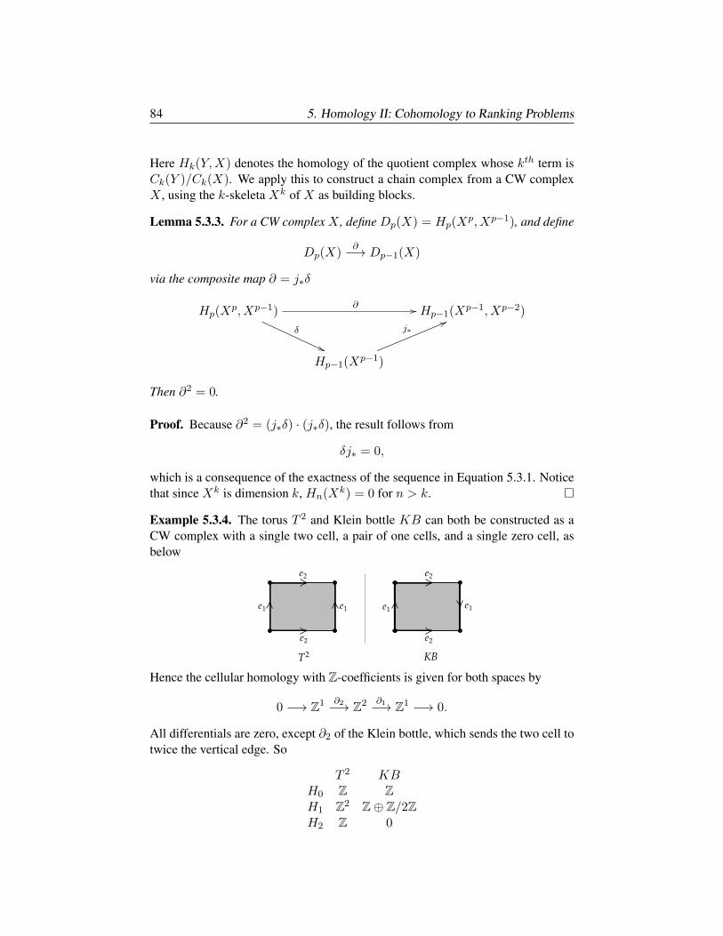
84 5. Homology II: Cohomology to Ranking Problems
Here Hk(Y,X) denotes the homology of the quotient complex whose kth term isCk(Y )/Ck(X). We apply this to construct a chain complex from a CW complexX , using the k-skeleta Xk of X as building blocks.
Lemma 5.3.3. For a CW complex X , define Dp(X) = Hp(Xp, Xp−1), and define
Dp(X)∂−→ Dp−1(X)
via the composite map ∂ = j∗δ
Hp(Xp, Xp−1)
∂ //
δ
((
Hp−1(Xp−1, Xp−2)
Hp−1(Xp−1)
j∗66
Then ∂2 = 0.
Proof. Because ∂2 = (j∗δ) · (j∗δ), the result follows from
δj∗ = 0,
which is a consequence of the exactness of the sequence in Equation 5.3.1. Noticethat since Xk is dimension k, Hn(Xk) = 0 for n > k.
Example 5.3.4. The torus T 2 and Klein bottle KB can both be constructed as aCW complex with a single two cell, a pair of one cells, and a single zero cell, asbelow
Hence the cellular homology with Z-coefficients is given for both spaces by
0 −→ Z1 ∂2−→ Z2 ∂1−→ Z1 −→ 0.
All differentials are zero, except ∂2 of the Klein bottle, which sends the two cell totwice the vertical edge. So
T 2 KBH0 Z ZH1 Z2 Z⊕ Z/2ZH2 Z 0
5.4. Poincare and Alexander Duality: Sensor Networks Revisited 85
5.4. Poincare and Alexander Duality: Sensor Networks Revisited
Henri Poincare discovered his duality theorem in 1893; it has an intrinsic appeal be-cause it concerns symmetry. In Poincare duality, there is a single underlying object(the manifold M ), and the duality involves the homology of M . James Alexanderproved his duality theorem in 1915; in contrast to Poincare duality, Alexander du-ality concerns two different spaces. Throughout this section the coefficient ring Rwill be a field K, and we sometimes write Hi(∗) for Hi(∗,K).
5.4.1. Statement of theorems and examples.
Theorem 5.4.1. [Poincare Duality] Let M be a compact, connected, orientablemanifold of dimension n without boundary. Then there is a perfect pairing
Hk(M)⊗Hn−k(M) −→ K.
This says that there is a vector space isomorphism HomK(Hn−k(M),K) ' Hk(M,K),which is often phrased in terms of cohomology
Hk(M,K) ' Hn−k(M,K).
Recall from §1 that for a simplicial complex ∆,
Ci(∆, R) = HomR(Ci(∆), R)
and that the simplicial cohomology H i(C ) is the cohomology at the ith position.The dimension bi of Hi(∆,K) is called the ith Betti number of ∆. So Poincareduality asserts that for M as in the statement of Theorem 5.4.1, the vector of Bettinumbers b(M)=(b0, . . . , bn) is a palindrome: (b0, . . . , bn)=(bn, . . . , b0).
Example 5.4.2. Our computations earlier in the chapter show that
b(S1) = (1, 1) by Example 4.2.5.b(S2) = (1, 0, 1) by Example 4.2.8.b(Sn) = (1, 0n−1, 1) by Example 5.3.2.
Example 5.3.4 showed that the Torus has Betti vector (1, 2, 1), whereas the KleinBottle has Betti vector (1, 1, 0). We don’t expect Poincare duality to hold for theKlein Bottle, since it is not orientable. However, see Example 5.4.19.
Theorem 5.4.3. [Alexander Duality] For a compact, locally contractible X ⊆ Sn,the homology of X and of Sn \X are related via
Hk(Sn \X) ' Hn−1−k(X)
where H i denotes reduced cohomology.
In terms of the reduced Betti vector, this says that b(Sn \X) is obtained by revers-ing b(X), then shifting left by one.
86 5. Homology II: Cohomology to Ranking Problems
Example 5.4.4. Let n = 2, with S2 triangulated as in ∆1 of Example 4.2.8, and letX be the subcomplex with maximal faces [1, 2], [2, 3], [3, 1], so X is homotopicto S1. The homology of X was computed in Example 4.2.5. Appending zeros sothe reduced Betti vector of X has length n+ 1 = 3 yields
b(X) = (0, 1, 0).
What about S2 \ X? Since singular and simplicial homology agree, we may usesingular homology to compute. As singular homology is homotopy invariant, re-moving the X = S1 “belt” from S2 results in two disconnected disks, which areeach homotopic to a point. Therefore b(S2 \X) = (2, 0, 0), hence
b(S2 \X) = (1, 0, 0)reverse (1, 0, 0) to obtain (0, 0, 1)
shift (0, 0, 1) left one step (0, 1, 0) = b(X).
5.4.2. Alexander Duality: Proof. We prove a combinatorial version of Alexan-der Duality, following the elegant argument of Bjorner–Tancer [17]. The setup isthe following: ∆ will be a simplicial complex on the vertex set V = v1, . . . , vn.We write S for the simplicial complex on V whose maximal faces correspond tothe subsets of V having n− 1 elements; therefore S is homotopic to Sn−2.
Definition 5.4.5. The combinatorial Alexander dual of ∆ is
∆∗ = σ ⊂ V | σ 6∈ ∆, where vi1 , . . . , vij = v1, . . . , vn \ vi1 , . . . , vij.The condition that σ 6∈ ∆ means that σ is not a face of ∆.
Example 5.4.6. For X in Example 5.4.4, the nonfaces of ∆ are
[1, 2, 3], [1, 2, 4], [1, 3, 4], [2, 3, 4], [1, 4], [2, 4], [3, 4], [4],so the complements of the nonfaces are
[4], [3], [2], [1], [2, 3], [1, 3], [1, 2], [1, 2, 3].Hence ∆∗ consists of the vertex [4] and the triangle [1, 2, 3], so ∆∗ is homotopic toa pair of points.
Since |V | = n, the corresponding sphere is an Sn−2, so combinatorial Alexanderduality will take the form
(5.4.1) Hi(∆) ' Hn−3−i(∆∗).
Lemma 5.4.7. For j ∈ σ ∈ ∆, sgn(j, σ) = (−1)i−1, where j is the ith smallestelement in the set σ. Let
p(σ) =∏i∈σ
(−1)i−1.
Then for k ∈ σ, sgn(k, σ)p(σ \ k) = sgn(k, σ ∪ k)p(σ).
Exercise 5.4.8. Show both sides of the expression above equal (−1)k−1.
5.4. Poincare and Alexander Duality: Sensor Networks Revisited 87
Let eσ ∈ Ci denote the element corresponding to σ ∈ ∆i, so that
(5.4.2) ∂i(eσ) =∑j∈σ
sgn(j, σ)eσ\j .
Dualizing to the Ci, this means the dual maps in cohomology are given by
(5.4.3) ∂i(e∗σ) =∑j 6∈σ
σ∪j∈∆
sgn(j, σ ∪ j)e∗σ∪j .
Equation 5.4.1 will follow from the following two isomorphisms, where 2V is thefull (solid) n− 1 simplex [v1, . . . , vn].
(5.4.4) Hi(∆) ' Hi+1(2V ,∆)
and
(5.4.5) Hi+1(2V ,∆) ' Hn−3−i(∆∗).
Equation 5.4.4 follows from the long exact sequence in relative homology for thepair ∆ ⊆ 2V , combined with all Hi(2
V ) = 0. The vanishing of Hi(2V ) for all i
follows since 2V is homotopic to a point. The key is showing Equation 5.4.5 holds.
Proof. (Combinatorial Alexander Duality–Equation 5.4.1) Write the differentialin relative homology for the pair (2V ,∆) as dj and the relative chains as Rj ; theoperator dj is given by essentially the same formula as Equation 5.4.2, except thatchains with image in Ci(∆) are zero; accounting for this we have:
(5.4.6) dj(eσ) =∑k∈σ
σ\k 6∈∆
sgn(k, σ)eσ\k.
Write Cj for relative cochains and dj for the relative coboundary operator, so that
(5.4.7) dj(e∗σ) =∑k 6∈σ
σ∪k∈∆∗
sgn(k, σ ∪ k)e∗σ∪k =∑k∈σ
σ\k 6∈∆
sgn(k, σ ∪ k)e∗σ\k.
To complete the proof we bring the operator p from Lemma 5.4.7 into play. Define
Rjφj−→ Cn−j−2 via φj(eσ) = p(σ)e∗σ.
Then the diagram
· · · // Rjdj //
φj
Rj−1
φj−1
// · · ·
· · · // Cn−2−j dn−1−j// Cn−j−1
// · · ·
commutes, and therefore induces the isomorphism of Equation 5.4.1.
Exercise 5.4.9. Check that indeed φj−1dj = dn−1−jφj .
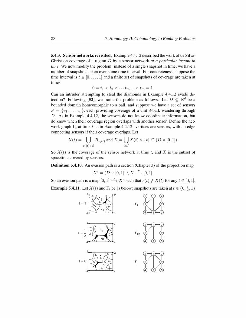
88 5. Homology II: Cohomology to Ranking Problems
5.4.3. Sensor networks revisited. Example 4.4.12 described the work of de Silva-Ghrist on coverage of a region D by a sensor network at a particular instant intime. We now modify the problem: instead of a single snapshot in time, we have anumber of snapshots taken over some time interval. For concreteness, suppose thetime interval is t ∈ [0, . . . , 1] and a finite set of snapshots of coverage are taken attimes
0 = t1 < t2 < · · · tm−1 < tm = 1.
Can an intruder attempting to steal the diamonds in Example 4.4.12 evade de-tection? Following [52], we frame the problem as follows. Let D ⊆ Rd be abounded domain homeomorphic to a ball, and suppose we have a set of sensorsS = v1, . . . , vn, each providing coverage of a unit d-ball, wandering throughD. As in Example 4.4.12, the sensors do not know coordinate information, butdo know when their coverage region overlaps with another sensor. Define the net-work graph Γt at time t as in Example 4.4.12: vertices are sensors, with an edgeconnecting sensors if their coverage overlaps. Let
X(t) =⋃
vi(t)∈S
Bvi(t) and X =⋃t∈I
X(t)× t ⊆ (D × [0, 1]).
So X(t) is the coverage of the sensor network at time t, and X is the subset ofspacetime covered by sensors.
Definition 5.4.10. An evasion path is a section (Chapter 3) of the projection map
Xc = (D × [0, 1]) \X π−→ [0, 1].
So an evasion path is a map [0, 1]s−→ Xc such that s(t) 6∈ X(t) for any t ∈ [0, 1].
Example 5.4.11. LetX(t) and Γt be as below: snapshots are taken at t ∈ 0, 12 , 1
1 6 2
75
4 8 3
1 6 2
75
4 8 3
1 6 2
75
4 8 3
1
1
1
8
2
2
2
3
3
34
4
4
5
5
5
6
6
6
7
7
7
8
8
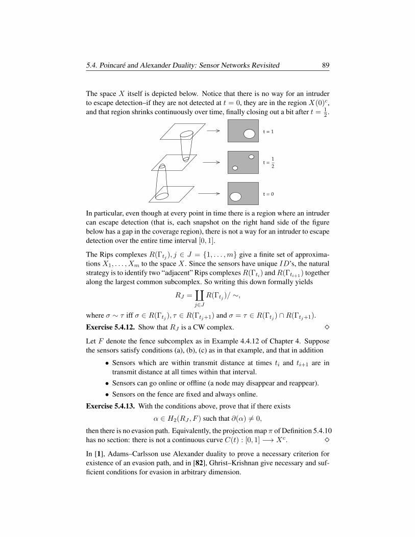
5.4. Poincare and Alexander Duality: Sensor Networks Revisited 89
The space X itself is depicted below. Notice that there is no way for an intruderto escape detection–if they are not detected at t = 0, they are in the region X(0)c,and that region shrinks continuously over time, finally closing out a bit after t = 1
2 .
In particular, even though at every point in time there is a region where an intrudercan escape detection (that is, each snapshot on the right hand side of the figurebelow has a gap in the coverage region), there is not a way for an intruder to escapedetection over the entire time interval [0, 1].
The Rips complexes R(Γtj ), j ∈ J = 1, . . . ,m give a finite set of approxima-tions X1, . . . , Xm to the space X . Since the sensors have unique ID’s, the naturalstrategy is to identify two “adjacent” Rips complexesR(Γti) andR(Γti+1) togetheralong the largest common subcomplex. So writing this down formally yields
RJ =∐j∈J
R(Γtj )/ ∼,
where σ ∼ τ iff σ ∈ R(Γtj ), τ ∈ R(Γtj+1) and σ = τ ∈ R(Γtj ) ∩R(Γtj+1).
Exercise 5.4.12. Show that RJ is a CW complex. Let F denote the fence subcomplex as in Example 4.4.12 of Chapter 4. Supposethe sensors satisfy conditions (a), (b), (c) as in that example, and that in addition
• Sensors which are within transmit distance at times ti and ti+1 are intransmit distance at all times within that interval.
• Sensors can go online or offline (a node may disappear and reappear).
• Sensors on the fence are fixed and always online.
Exercise 5.4.13. With the conditions above, prove that if there exists
α ∈ H2(RJ , F ) such that ∂(α) 6= 0,
then there is no evasion path. Equivalently, the projection map π of Definition 5.4.10has no section: there is not a continuous curve C(t) : [0, 1] −→ Xc. In [1], Adams–Carlsson use Alexander duality to prove a necessary criterion forexistence of an evasion path, and in [82], Ghrist–Krishnan give necessary and suf-ficient conditions for evasion in arbitrary dimension.
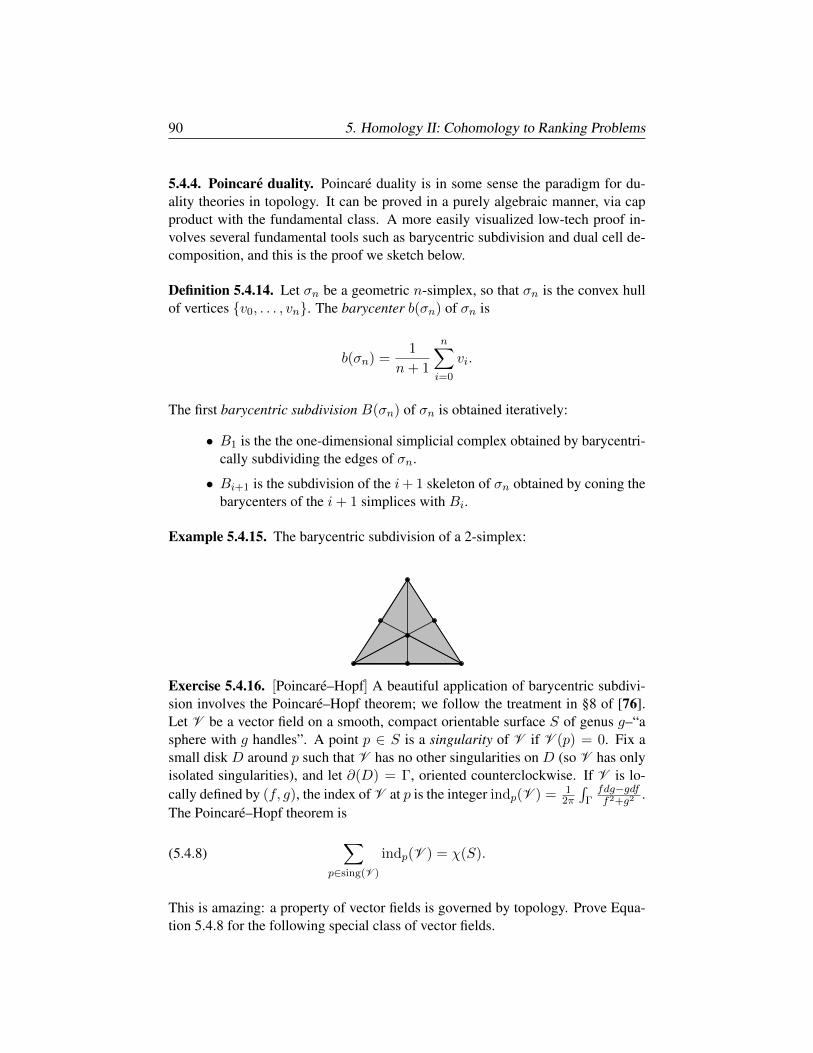
90 5. Homology II: Cohomology to Ranking Problems
5.4.4. Poincare duality. Poincare duality is in some sense the paradigm for du-ality theories in topology. It can be proved in a purely algebraic manner, via capproduct with the fundamental class. A more easily visualized low-tech proof in-volves several fundamental tools such as barycentric subdivision and dual cell de-composition, and this is the proof we sketch below.
Definition 5.4.14. Let σn be a geometric n-simplex, so that σn is the convex hullof vertices v0, . . . , vn. The barycenter b(σn) of σn is
b(σn) =1
n+ 1
n∑i=0
vi.
The first barycentric subdivision B(σn) of σn is obtained iteratively:
• B1 is the the one-dimensional simplicial complex obtained by barycentri-cally subdividing the edges of σn.
• Bi+1 is the subdivision of the i+ 1 skeleton of σn obtained by coning thebarycenters of the i+ 1 simplices with Bi.
Example 5.4.15. The barycentric subdivision of a 2-simplex:
Exercise 5.4.16. [Poincare–Hopf] A beautiful application of barycentric subdivi-sion involves the Poincare–Hopf theorem; we follow the treatment in §8 of [76].Let V be a vector field on a smooth, compact orientable surface S of genus g–“asphere with g handles”. A point p ∈ S is a singularity of V if V (p) = 0. Fix asmall disk D around p such that V has no other singularities on D (so V has onlyisolated singularities), and let ∂(D) = Γ, oriented counterclockwise. If V is lo-cally defined by (f, g), the index of V at p is the integer indp(V ) = 1
2π
∫Γfdg−gdff2+g2 .
The Poincare–Hopf theorem is
(5.4.8)∑
p∈sing(V )
indp(V ) = χ(S).
This is amazing: a property of vector fields is governed by topology. Prove Equa-tion 5.4.8 for the following special class of vector fields.
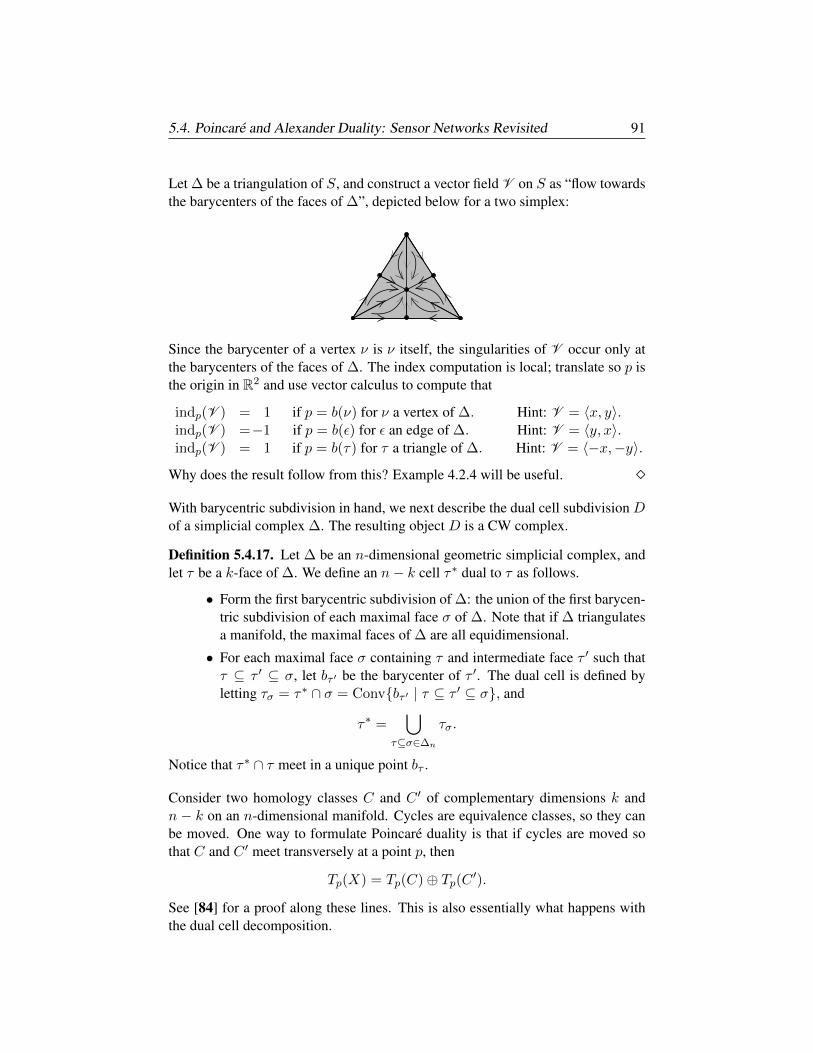
5.4. Poincare and Alexander Duality: Sensor Networks Revisited 91
Let ∆ be a triangulation of S, and construct a vector field V on S as “flow towardsthe barycenters of the faces of ∆”, depicted below for a two simplex:
Since the barycenter of a vertex ν is ν itself, the singularities of V occur only atthe barycenters of the faces of ∆. The index computation is local; translate so p isthe origin in R2 and use vector calculus to compute that
indp(V ) = 1 if p = b(ν) for ν a vertex of ∆. Hint: V = 〈x, y〉.indp(V ) =−1 if p = b(ε) for ε an edge of ∆. Hint: V = 〈y, x〉.indp(V ) = 1 if p = b(τ) for τ a triangle of ∆. Hint: V = 〈−x,−y〉.
Why does the result follow from this? Example 4.2.4 will be useful.
With barycentric subdivision in hand, we next describe the dual cell subdivision Dof a simplicial complex ∆. The resulting object D is a CW complex.
Definition 5.4.17. Let ∆ be an n-dimensional geometric simplicial complex, andlet τ be a k-face of ∆. We define an n− k cell τ∗ dual to τ as follows.
• Form the first barycentric subdivision of ∆: the union of the first barycen-tric subdivision of each maximal face σ of ∆. Note that if ∆ triangulatesa manifold, the maximal faces of ∆ are all equidimensional.
• For each maximal face σ containing τ and intermediate face τ ′ such thatτ ⊆ τ ′ ⊆ σ, let bτ ′ be the barycenter of τ ′. The dual cell is defined byletting τσ = τ∗ ∩ σ = Convbτ ′ | τ ⊆ τ ′ ⊆ σ, and
τ∗ =⋃
τ⊆σ∈∆n
τσ.
Notice that τ∗ ∩ τ meet in a unique point bτ .
Consider two homology classes C and C ′ of complementary dimensions k andn − k on an n-dimensional manifold. Cycles are equivalence classes, so they canbe moved. One way to formulate Poincare duality is that if cycles are moved sothat C and C ′ meet transversely at a point p, then
Tp(X) = Tp(C)⊕ Tp(C ′).
See [84] for a proof along these lines. This is also essentially what happens withthe dual cell decomposition.
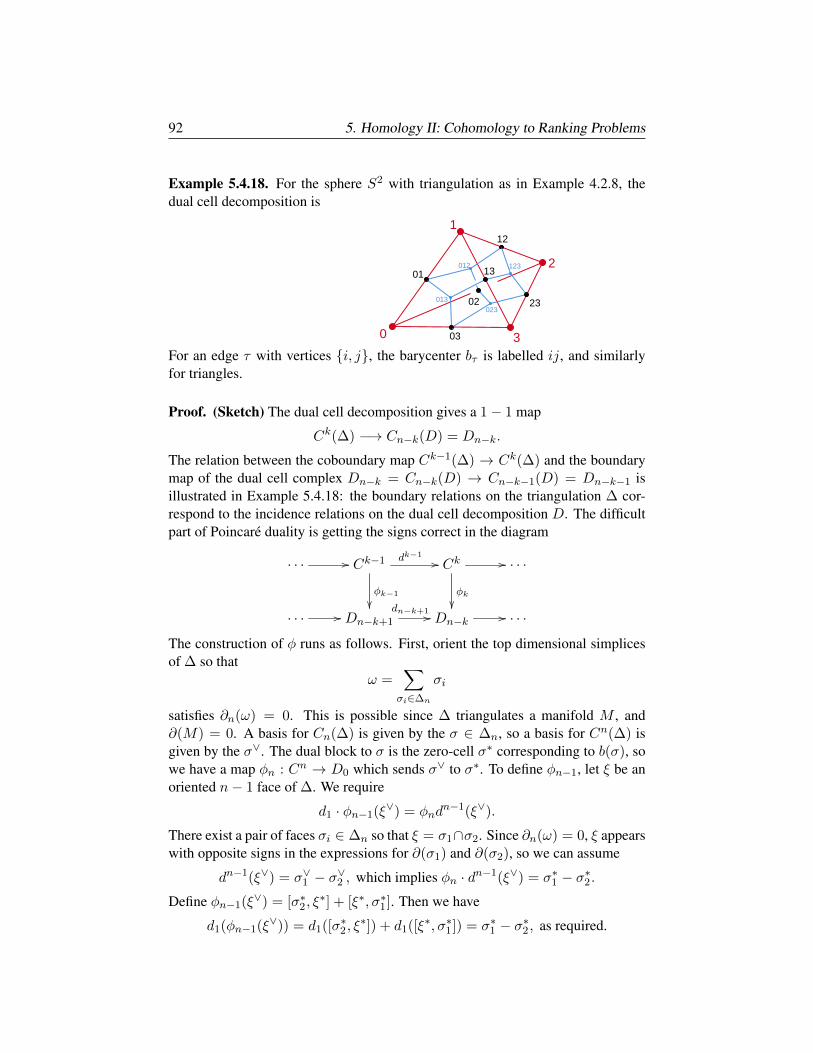
92 5. Homology II: Cohomology to Ranking Problems
Example 5.4.18. For the sphere S2 with triangulation as in Example 4.2.8, thedual cell decomposition is
03
12
01
23
0
1
2
3
012
023
123
013
13
02
For an edge τ with vertices i, j, the barycenter bτ is labelled ij, and similarlyfor triangles.
Proof. (Sketch) The dual cell decomposition gives a 1− 1 map
Ck(∆) −→ Cn−k(D) = Dn−k.
The relation between the coboundary map Ck−1(∆) → Ck(∆) and the boundarymap of the dual cell complex Dn−k = Cn−k(D) → Cn−k−1(D) = Dn−k−1 isillustrated in Example 5.4.18: the boundary relations on the triangulation ∆ cor-respond to the incidence relations on the dual cell decomposition D. The difficultpart of Poincare duality is getting the signs correct in the diagram
· · · // Ck−1 dk−1//
φk−1
Ck
φk
// · · ·
· · · // Dn−k+1
dn−k+1 // Dn−k // · · ·
The construction of φ runs as follows. First, orient the top dimensional simplicesof ∆ so that
ω =∑σi∈∆n
σi
satisfies ∂n(ω) = 0. This is possible since ∆ triangulates a manifold M , and∂(M) = 0. A basis for Cn(∆) is given by the σ ∈ ∆n, so a basis for Cn(∆) isgiven by the σ∨. The dual block to σ is the zero-cell σ∗ corresponding to b(σ), sowe have a map φn : Cn → D0 which sends σ∨ to σ∗. To define φn−1, let ξ be anoriented n− 1 face of ∆. We require
d1 · φn−1(ξ∨) = φndn−1(ξ∨).
There exist a pair of faces σi ∈ ∆n so that ξ = σ1∩σ2. Since ∂n(ω) = 0, ξ appearswith opposite signs in the expressions for ∂(σ1) and ∂(σ2), so we can assume
dn−1(ξ∨) = σ∨1 − σ∨2 , which implies φn · dn−1(ξ∨) = σ∗1 − σ∗2.Define φn−1(ξ∨) = [σ∗2, ξ
∗] + [ξ∗, σ∗1]. Then we have
d1(φn−1(ξ∨)) = d1([σ∗2, ξ∗]) + d1([ξ∗, σ∗1]) = σ∗1 − σ∗2, as required.
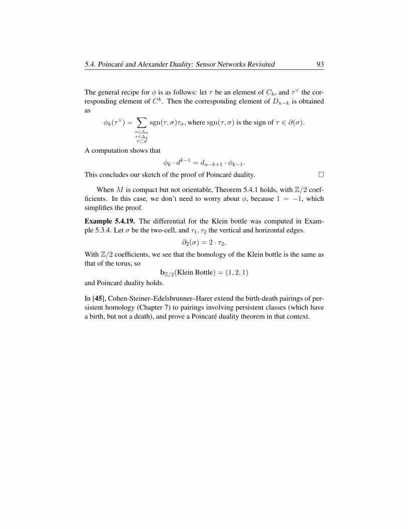
5.4. Poincare and Alexander Duality: Sensor Networks Revisited 93
The general recipe for φ is as follows: let τ be an element of Ck, and τ∨ the cor-responding element of Ck. Then the corresponding element of Dn−k is obtainedas
φk(τ∨) =
∑σ∈∆nτ∈∆kτ⊂σ
sgn(τ, σ)τσ,where sgn(τ, σ) is the sign of τ ∈ ∂(σ).
A computation shows that
φk · dk−1 = dn−k+1 · φk−1.
This concludes our sketch of the proof of Poincare duality.
When M is compact but not orientable, Theorem 5.4.1 holds, with Z/2 coef-ficients. In this case, we don’t need to worry about φ, because 1 = −1, whichsimplifies the proof.
Example 5.4.19. The differential for the Klein bottle was computed in Exam-ple 5.3.4. Let σ be the two-cell, and τ1, τ2 the vertical and horizontal edges.
∂2(σ) = 2 · τ2,
With Z/2 coefficients, we see that the homology of the Klein bottle is the same asthat of the torus, so
bZ/2(Klein Bottle) = (1, 2, 1)
and Poincare duality holds.
In [45], Cohen-Steiner–Edelsbrunner–Harer extend the birth-death pairings of per-sistent homology (Chapter 7) to pairings involving persistent classes (which havea birth, but not a death), and prove a Poincare duality theorem in that context.

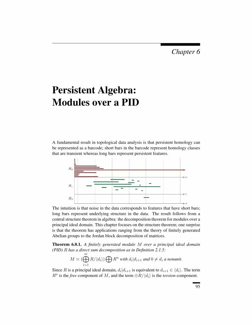
Chapter 6
Persistent Algebra:Modules over a PID
A fundamental result in topological data analysis is that persistent homology canbe represented as a barcode; short bars in the barcode represent homology classesthat are transient whereas long bars represent persistent features.
The intuition is that noise in the data corresponds to features that have short bars;long bars represent underlying structure in the data. The result follows from acentral structure theorem in algebra: the decomposition theorem for modules over aprincipal ideal domain. This chapter focuses on the structure theorem; one surpriseis that the theorem has applications ranging from the theory of finitely generatedAbelian groups to the Jordan block decomposition of matrices.
Theorem 6.0.1. A finitely generated module M over a principal ideal domain(PID) R has a direct sum decomposition as in Definition 2.1.5:
M ' (
m⊕i=1
R/〈di〉)⊕
Rn with di|di+1 and 0 6= di a nonunit.
Since R is a principal ideal domain, di|di+1 is equivalent to di+1 ∈ 〈di〉. The termRn is the free component of M , and the term ⊕R/〈di〉 is the torsion component.
95
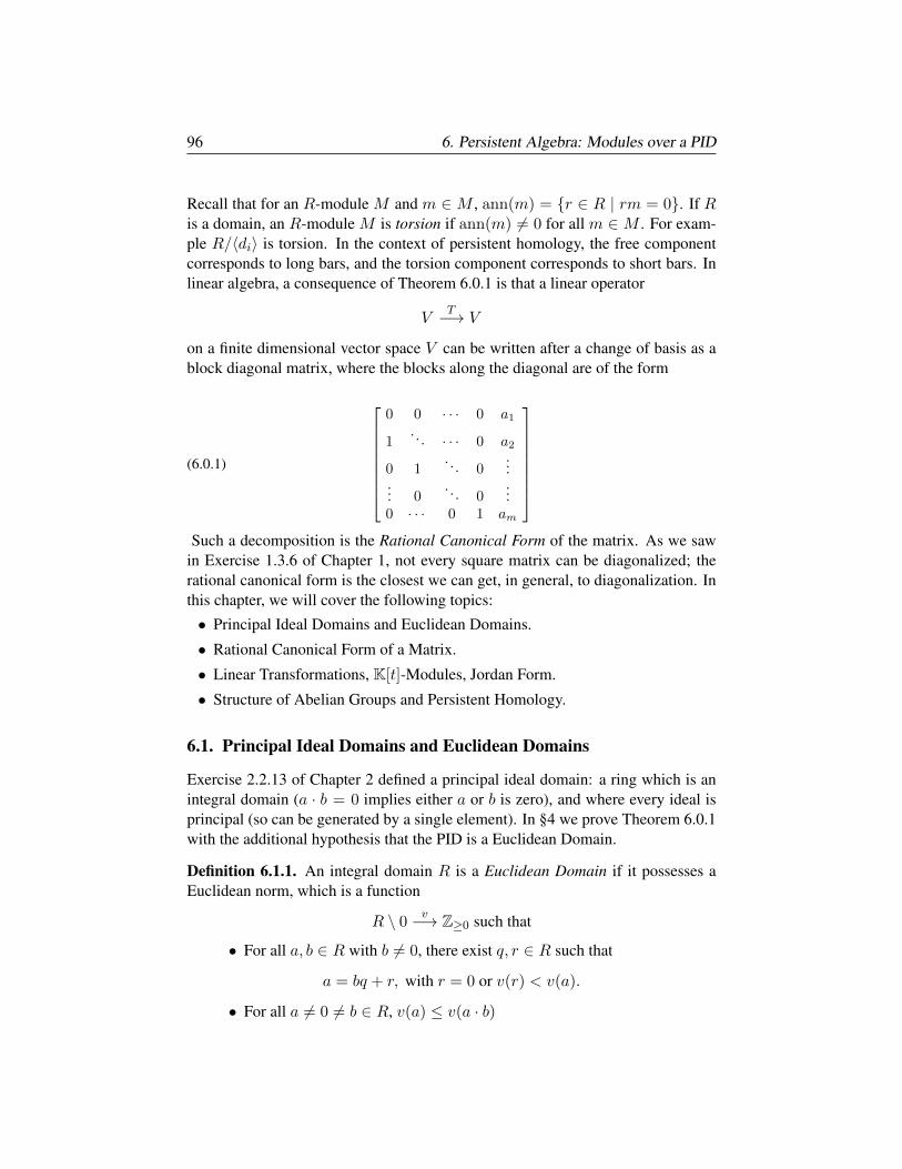
96 6. Persistent Algebra: Modules over a PID
Recall that for an R-module M and m ∈ M , ann(m) = r ∈ R | rm = 0. If Ris a domain, an R-module M is torsion if ann(m) 6= 0 for all m ∈ M . For exam-ple R/〈di〉 is torsion. In the context of persistent homology, the free componentcorresponds to long bars, and the torsion component corresponds to short bars. Inlinear algebra, a consequence of Theorem 6.0.1 is that a linear operator
VT−→ V
on a finite dimensional vector space V can be written after a change of basis as ablock diagonal matrix, where the blocks along the diagonal are of the form
(6.0.1)
0 0 · · · 0 a1
1. . . · · · 0 a2
0 1. . . 0
...... 0
. . . 0...
0 · · · 0 1 am
Such a decomposition is the Rational Canonical Form of the matrix. As we saw
in Exercise 1.3.6 of Chapter 1, not every square matrix can be diagonalized; therational canonical form is the closest we can get, in general, to diagonalization. Inthis chapter, we will cover the following topics:
• Principal Ideal Domains and Euclidean Domains.
• Rational Canonical Form of a Matrix.
• Linear Transformations, K[t]-Modules, Jordan Form.
• Structure of Abelian Groups and Persistent Homology.
6.1. Principal Ideal Domains and Euclidean Domains
Exercise 2.2.13 of Chapter 2 defined a principal ideal domain: a ring which is anintegral domain (a · b = 0 implies either a or b is zero), and where every ideal isprincipal (so can be generated by a single element). In §4 we prove Theorem 6.0.1with the additional hypothesis that the PID is a Euclidean Domain.
Definition 6.1.1. An integral domain R is a Euclidean Domain if it possesses aEuclidean norm, which is a function
R \ 0v−→ Z≥0 such that
• For all a, b ∈ R with b 6= 0, there exist q, r ∈ R such that
a = bq + r, with r = 0 or v(r) < v(a).
• For all a 6= 0 6= b ∈ R, v(a) ≤ v(a · b)
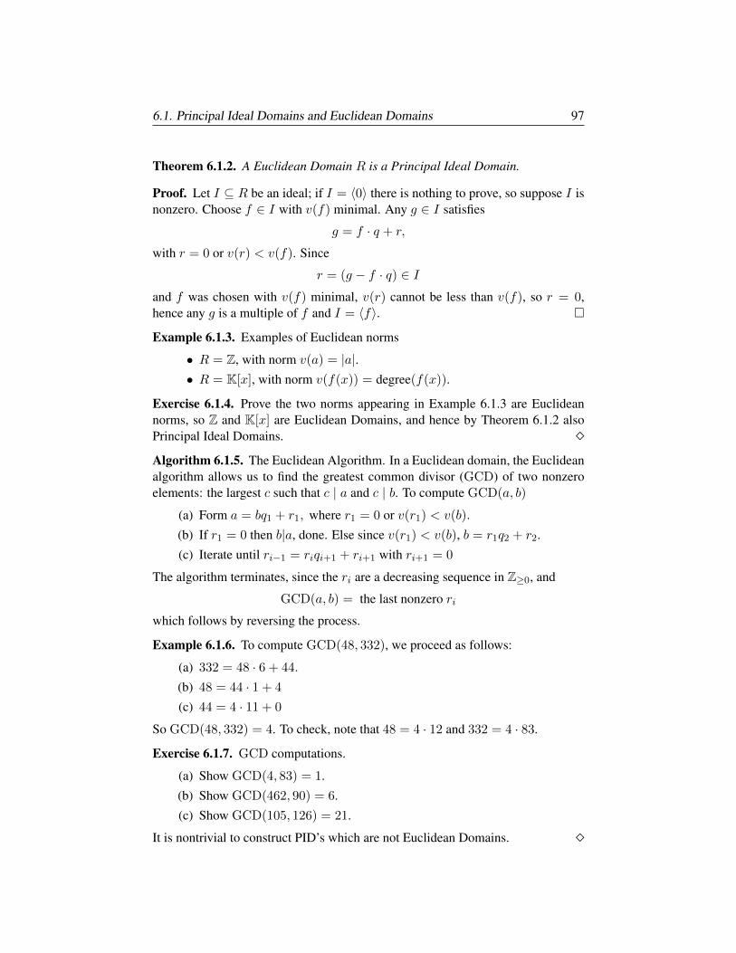
6.1. Principal Ideal Domains and Euclidean Domains 97
Theorem 6.1.2. A Euclidean Domain R is a Principal Ideal Domain.
Proof. Let I ⊆ R be an ideal; if I = 〈0〉 there is nothing to prove, so suppose I isnonzero. Choose f ∈ I with v(f) minimal. Any g ∈ I satisfies
g = f · q + r,
with r = 0 or v(r) < v(f). Since
r = (g − f · q) ∈ Iand f was chosen with v(f) minimal, v(r) cannot be less than v(f), so r = 0,hence any g is a multiple of f and I = 〈f〉.
Example 6.1.3. Examples of Euclidean norms
• R = Z, with norm v(a) = |a|.• R = K[x], with norm v(f(x)) = degree(f(x)).
Exercise 6.1.4. Prove the two norms appearing in Example 6.1.3 are Euclideannorms, so Z and K[x] are Euclidean Domains, and hence by Theorem 6.1.2 alsoPrincipal Ideal Domains. Algorithm 6.1.5. The Euclidean Algorithm. In a Euclidean domain, the Euclideanalgorithm allows us to find the greatest common divisor (GCD) of two nonzeroelements: the largest c such that c | a and c | b. To compute GCD(a, b)
(a) Form a = bq1 + r1, where r1 = 0 or v(r1) < v(b).
(b) If r1 = 0 then b|a, done. Else since v(r1) < v(b), b = r1q2 + r2.
(c) Iterate until ri−1 = riqi+1 + ri+1 with ri+1 = 0
The algorithm terminates, since the ri are a decreasing sequence in Z≥0, and
GCD(a, b) = the last nonzero ri
which follows by reversing the process.
Example 6.1.6. To compute GCD(48, 332), we proceed as follows:
(a) 332 = 48 · 6 + 44.
(b) 48 = 44 · 1 + 4
(c) 44 = 4 · 11 + 0
So GCD(48, 332) = 4. To check, note that 48 = 4 · 12 and 332 = 4 · 83.
Exercise 6.1.7. GCD computations.
(a) Show GCD(4, 83) = 1.
(b) Show GCD(462, 90) = 6.
(c) Show GCD(105, 126) = 21.
It is nontrivial to construct PID’s which are not Euclidean Domains.
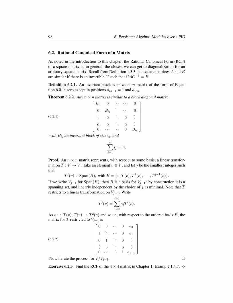
98 6. Persistent Algebra: Modules over a PID
6.2. Rational Canonical Form of a Matrix
As noted in the introduction to this chapter, the Rational Canonical Form (RCF)of a square matrix is, in general, the closest we can get to diagonalization for anarbitrary square matrix. Recall from Definition 1.3.3 that square matrices A and Bare similar if there is an invertible C such that CAC−1 = B.
Definition 6.2.1. An invariant block is an m × m matrix of the form of Equa-tion 6.0.1: zero except in positions ai,i−1 = 1 and ai,m.
Theorem 6.2.2. Any n× n matrix is similar to a block diagonal matrix
(6.2.1)
Bi1 0 · · · · · · 0
0 Bi2. . . · · · 0
... 0. . . 0
...
0 0. . . 0
...0 · · · · · · 0 Bik
with Bij an invariant block of size ij , and
k∑j=1
ij = n.
Proof. An n × n matrix represents, with respect to some basis, a linear transfor-mation T : V → V . Take an element v ∈ V , and let j be the smallest integer suchthat
T j(v) ∈ Span(B), with B = v, T (v), T 2(v), · · · , T j−1(v).If we write Vj−1 for Span(B), then B is a basis for Vj−1: by construction it is aspanning set, and linearly independent by the choice of j as minimal. Note that Trestricts to a linear transformation on Vj−1. Write
T j(v) =
j−1∑i=0
aiTi(v).
As v 7→ T (v), T (v) 7→ T 2(v) and so on, with respect to the ordered basis B, thematrix for T restricted to Vj−1 is
(6.2.2)
0 0 · · · 0 a0
1. . . · · · 0 a1
0 1. . . 0
...... 0
. . . 0...
0 · · · 0 1 aj−1
Now iterate the process for V/Vj−1.
Exercise 6.2.3. Find the RCF of the 4× 4 matrix in Chapter 1, Example 1.4.7.
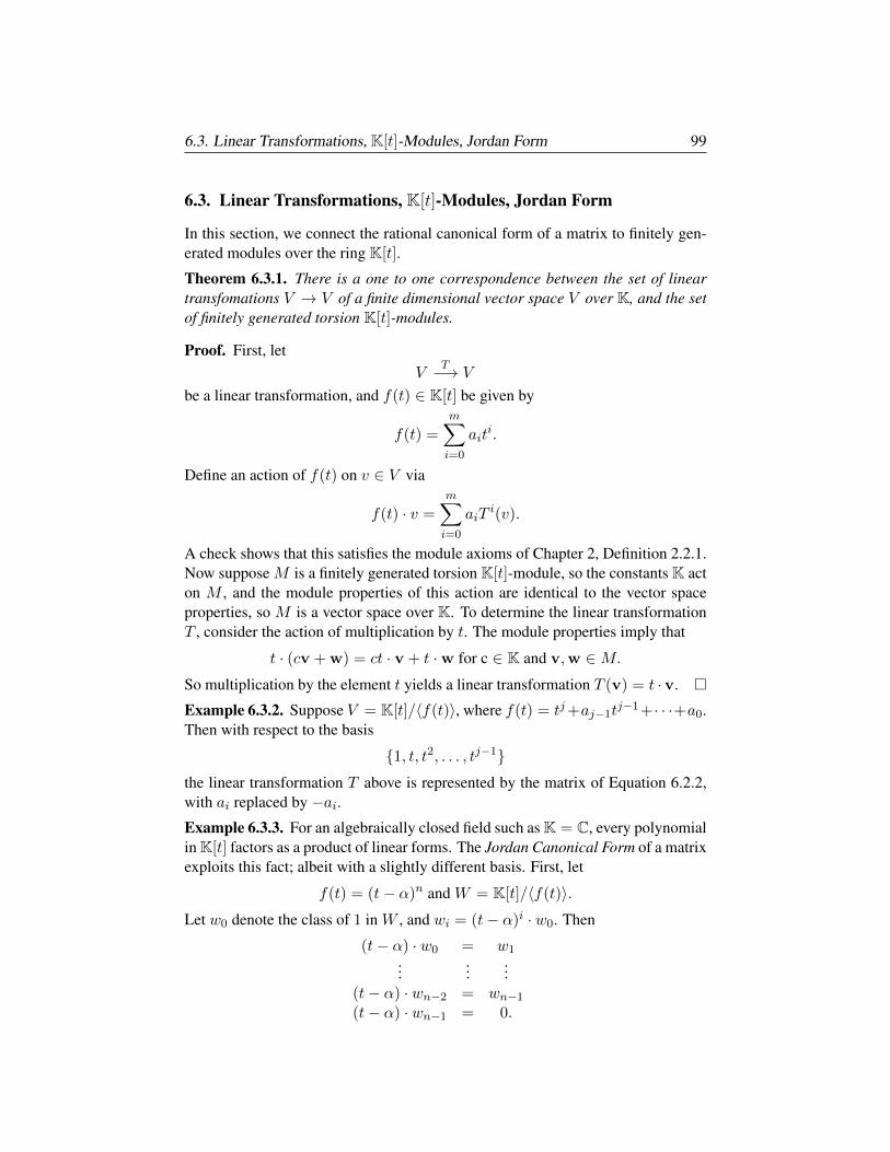
6.3. Linear Transformations, K[t]-Modules, Jordan Form 99
6.3. Linear Transformations, K[t]-Modules, Jordan Form
In this section, we connect the rational canonical form of a matrix to finitely gen-erated modules over the ring K[t].
Theorem 6.3.1. There is a one to one correspondence between the set of lineartransfomations V → V of a finite dimensional vector space V over K, and the setof finitely generated torsion K[t]-modules.
Proof. First, letV
T−→ V
be a linear transformation, and f(t) ∈ K[t] be given by
f(t) =m∑i=0
aiti.
Define an action of f(t) on v ∈ V via
f(t) · v =m∑i=0
aiTi(v).
A check shows that this satisfies the module axioms of Chapter 2, Definition 2.2.1.Now suppose M is a finitely generated torsion K[t]-module, so the constants K acton M , and the module properties of this action are identical to the vector spaceproperties, so M is a vector space over K. To determine the linear transformationT , consider the action of multiplication by t. The module properties imply that
t · (cv + w) = ct · v + t ·w for c ∈ K and v,w ∈M.
So multiplication by the element t yields a linear transformation T (v) = t ·v.
Example 6.3.2. Suppose V = K[t]/〈f(t)〉, where f(t) = tj+aj−1tj−1+· · ·+a0.
Then with respect to the basis
1, t, t2, . . . , tj−1the linear transformation T above is represented by the matrix of Equation 6.2.2,with ai replaced by −ai.Example 6.3.3. For an algebraically closed field such as K = C, every polynomialin K[t] factors as a product of linear forms. The Jordan Canonical Form of a matrixexploits this fact; albeit with a slightly different basis. First, let
f(t) = (t− α)n and W = K[t]/〈f(t)〉.Let w0 denote the class of 1 in W , and wi = (t− α)i · w0. Then
(t− α) · w0 = w1...
......
(t− α) · wn−2 = wn−1
(t− α) · wn−1 = 0.
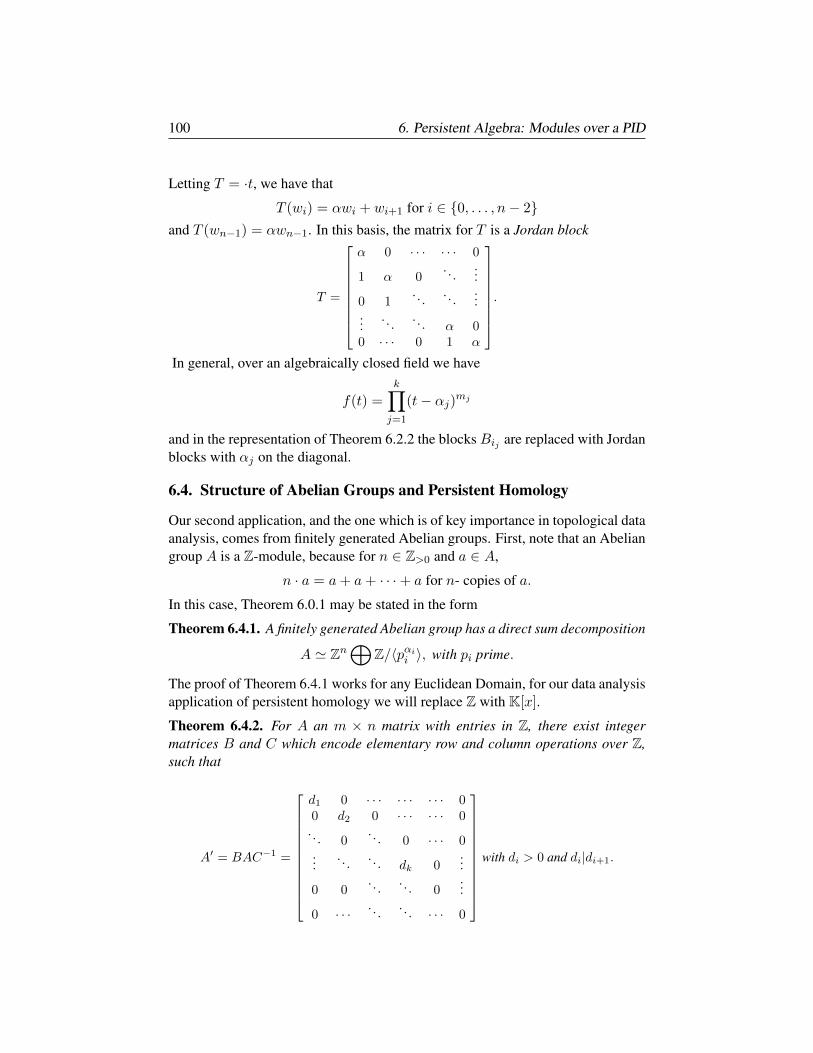
100 6. Persistent Algebra: Modules over a PID
Letting T = ·t, we have that
T (wi) = αwi + wi+1 for i ∈ 0, . . . , n− 2and T (wn−1) = αwn−1. In this basis, the matrix for T is a Jordan block
T =
α 0 · · · · · · 0
1 α 0. . .
...
0 1. . . . . .
......
. . . . . . α 00 · · · 0 1 α
.
In general, over an algebraically closed field we have
f(t) =k∏j=1
(t− αj)mj
and in the representation of Theorem 6.2.2 the blocks Bij are replaced with Jordanblocks with αj on the diagonal.
6.4. Structure of Abelian Groups and Persistent Homology
Our second application, and the one which is of key importance in topological dataanalysis, comes from finitely generated Abelian groups. First, note that an Abeliangroup A is a Z-module, because for n ∈ Z>0 and a ∈ A,
n · a = a+ a+ · · ·+ a for n- copies of a.
In this case, Theorem 6.0.1 may be stated in the form
Theorem 6.4.1. A finitely generated Abelian group has a direct sum decomposition
A ' Zn⊕
Z/〈pαii 〉, with pi prime.
The proof of Theorem 6.4.1 works for any Euclidean Domain, for our data analysisapplication of persistent homology we will replace Z with K[x].
Theorem 6.4.2. For A an m × n matrix with entries in Z, there exist integermatrices B and C which encode elementary row and column operations over Z,such that
A′ = BAC−1 =
d1 0 · · · · · · · · · 00 d2 0 · · · · · · 0. . . 0
. . . 0 · · · 0...
. . .. . . dk 0
...
0 0. . .
. . . 0...
0 · · ·. . .
. . . · · · 0
with di > 0 and di|di+1.
6.4. Structure of Abelian Groups and Persistent Homology 101
Proof. The proof has two steps, and moves back and forth between them:
(a) We first use elementary row and column swaps to put the smallest entryof A in position (1, 1). Next, use elementary row and column operationsto zero out all entries in the first row and column, except at position (1, 1).When the entries of A are in a field K, this is straightforward, but over Zcare must be taken. For example, if the first row starts as [2, 3, · · · ], wecan use 2 to reduce 3, with a remainder of 1. Now 1 is the smallest entry,so swap it into position (1, 1), and continue.
The key point is that each entry in the first row may be written as
a1i = a11q + r, with r = 0 or r < a11.
If r = 0 then a1i reduces to zero mod a11. Otherwise after reducinga1i = r, swap the first column and column i to get the smaller value r inposition (1, 1). This process concludes with a matrix A′ which is nonzeroin the first row and first column only in position (1, 1), with A′1,1 = d1.To achieve di|di+1, we need to do more work.
(b) SupposeA′ has an entry b which is not divisible by d1. Add the column ofA′ containing b to the first column of A′, and call the resulting matrix A′′.Because the column of A′ containing b has zero entry in the first row, andthe first column of A′ is zero except in position (1, 1), the first column ofA′′ has b as an entry. Since a11 = d1 does not divide b, we have
b = a11q + r with r 6= 0, so r < a11.
Swap the row with r with the first row, and return to step (a).
The process terminates: at every step, the numbers decrease in absolute value.
Exercise 6.4.3. Working with Z/p.
(a) Show thatZ/2× Z/2 6' Z/4.
(b) Show that if p1 and p2 are distinct prime numbers, then
Z/p1 × Z/p2 ' Z/p1p2.
Now show that Theorem 6.4.1 is equivalent to Theorem 6.4.2. Lemma 6.4.4. If R is a Noetherian ring and M a finitely generated R-module,then the module of relations F in Definition 2.2.20 of Chapter 2 is of finite rank.
Proof. Exercise 2.4.4 of Chapter 2 shows that a finitely generated module over aNoetherian ring is Noetherian, hence so is every submodule.
With these preliminaries in hand, we’re ready for the proof of Theorem 6.4.1.
102 6. Persistent Algebra: Modules over a PID
Proof [of Theorem 6.4.1] If A is a finitely generated Abelian group, then A is afinitely generated Z-module. As a principal ideal domain is Noetherian, Lemma 6.4.4implies that A has a presentation of the form
Zm φ−→ Zn −→ A −→ 0.
By Theorem 6.4.2,
φ =
d1 0 · · · · · · · · · 00 d2 0 · · · · · · 0. . . 0
. . . 0 · · · 0...
. . . . . . dk 0...
0 0. . . . . . 0
...
0 · · ·. . . . . . · · · 0
with di > 0 and di|di+1.
Since A = coker(φ), this means exactly that A '( k⊕i=1
Z/diZ)⊕
Zn−k.
For a Euclidean domain, Theorem 6.4.1 and Theorem 6.0.1 are equivalent, andwith small modifications this proof also works for a PID.
Exercise 6.4.5. Row reduce the matrix 3 1 −42 −3 1−4 6 −2
using integer elementary operations. 6.4.1. Z-graded rings. Chapter 7 introduces persistent homology, where the al-gebraic invariants that are constructed are modules over K[x]. Since K[x] is aEuclidean Domain, we can apply Theorem 6.4.1 to analyze the structure of theresulting modules. In fact, K[x] has additional structure: it is a Z-graded ring:
Definition 6.4.6. A ring R is Z-graded if R = ⊕i∈ZRi, such that if ri ∈ Ri andrj ∈ Rj , ri · rj ∈ Ri+j . Note that if R0 = K then all the Ri are K-vector spaces.A Z-graded module M over a Z-graded ring R must satisfy a similar condition
M =⊕i∈Z
Mi, and if m ∈Mi and rj ∈ Rj then rj ·mi ∈Mi+j .
We write R(i) for a free module of rank one, with generator in degree −i. There-fore R(i)j ' Ri+j , in particular, R(−i)i ' R0.
Exercise 6.4.7. For R = K[x], R(−2) is a free module with unit appearing indegree 2, and so multiplication by x2 defines a graded map R→ R(2). Show thatfor R = K[x1, . . . , xn] the multiplication by f(x1, . . . , xn) defines a graded maponly when f is a homogeneous polynomial as in Exercise 2.4.16. Grading plays a key role in persistent homology, and is discussed in detail in §8.2.
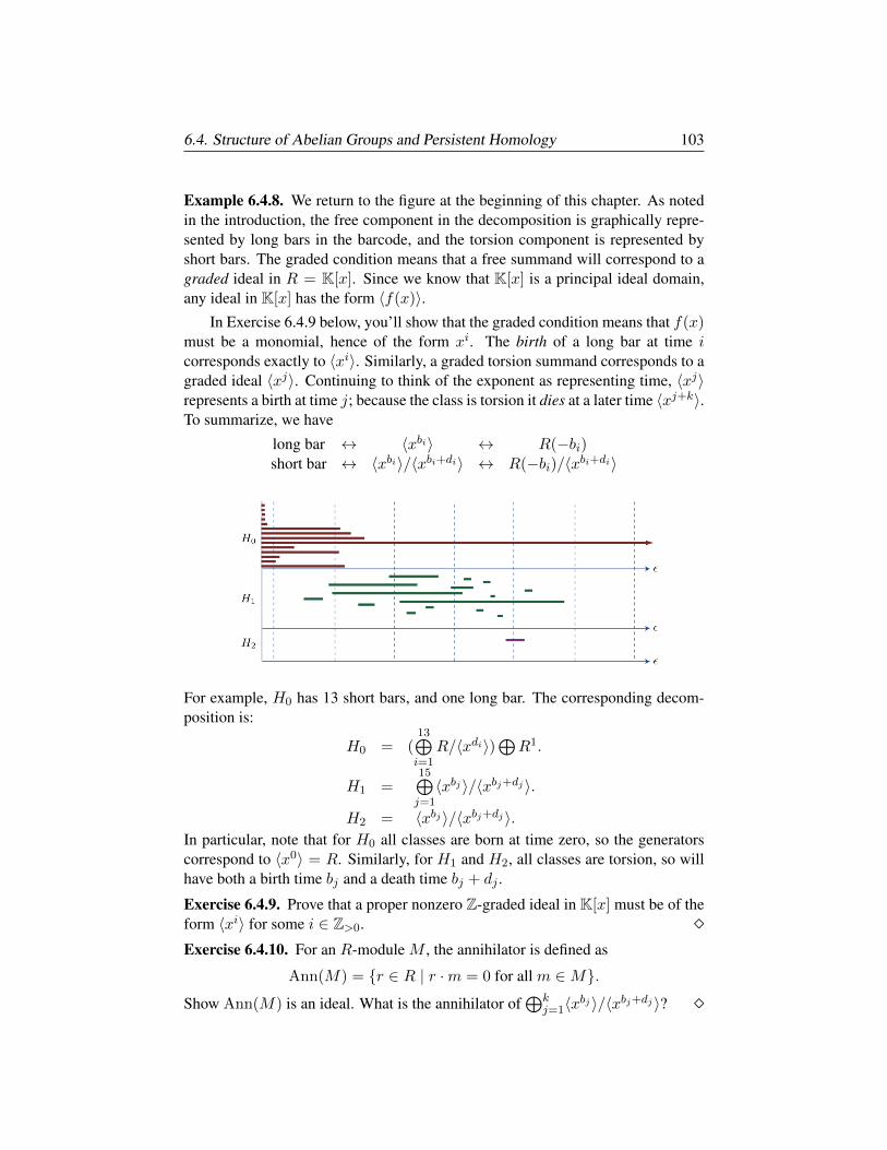
6.4. Structure of Abelian Groups and Persistent Homology 103
Example 6.4.8. We return to the figure at the beginning of this chapter. As notedin the introduction, the free component in the decomposition is graphically repre-sented by long bars in the barcode, and the torsion component is represented byshort bars. The graded condition means that a free summand will correspond to agraded ideal in R = K[x]. Since we know that K[x] is a principal ideal domain,any ideal in K[x] has the form 〈f(x)〉.
In Exercise 6.4.9 below, you’ll show that the graded condition means that f(x)must be a monomial, hence of the form xi. The birth of a long bar at time icorresponds exactly to 〈xi〉. Similarly, a graded torsion summand corresponds to agraded ideal 〈xj〉. Continuing to think of the exponent as representing time, 〈xj〉represents a birth at time j; because the class is torsion it dies at a later time 〈xj+k〉.To summarize, we have
long bar ↔ 〈xbi〉 ↔ R(−bi)short bar ↔ 〈xbi〉/〈xbi+di〉 ↔ R(−bi)/〈xbi+di〉
For example, H0 has 13 short bars, and one long bar. The corresponding decom-position is:
H0 = (13⊕i=1
R/〈xdi〉)⊕R1.
H1 =15⊕j=1〈xbj 〉/〈xbj+dj 〉.
H2 = 〈xbj 〉/〈xbj+dj 〉.In particular, note that for H0 all classes are born at time zero, so the generatorscorrespond to 〈x0〉 = R. Similarly, for H1 and H2, all classes are torsion, so willhave both a birth time bj and a death time bj + dj .
Exercise 6.4.9. Prove that a proper nonzero Z-graded ideal in K[x] must be of theform 〈xi〉 for some i ∈ Z>0. Exercise 6.4.10. For an R-module M , the annihilator is defined as
Ann(M) = r ∈ R | r ·m = 0 for all m ∈M.
Show Ann(M) is an ideal. What is the annihilator of⊕k
j=1〈xbj 〉/〈xbj+dj 〉?

Chapter 7
Persistent Homology
We’re ready to reap the fruits of our labors in the previous chapters, and attack themotivating problem from the preface: given point cloud data X ⊆ Rn, we wantto extract meaning from X . In this chapter, we study persistent homology (PH),which can facilitate detection and analysis of underlying structure in large datasets.Persistent homology assigns a graded module over a principal ideal domain to a fil-tered simplicial complex. In Chapter 6, we proved that a finitely generated moduleM over a principal ideal domain R has a decomposition:
M ' (k⊕i=1
R/pi)⊕Rm
Persistent homology is often displayed as a barcode diagram. The decompositionabove translates into a barcode as follows: the free summands (which are known aslong bars) represent persistent features of the underlying data set, while the torsioncomponents (which are known as short bars) represent noise in the data. Thegrading allows us to assign birth and death times to homology classes. Persistenthomology has proven effective in a number of settings, including breast cancerpathology [28], viral evolution [37], and visual cortex activity [136], to name justa few. We start by using X as a seed from which to build a family of spaces
Xε =⋃p∈X
Nε(p), where Nε(p) denotes an ε ball around p.
AsXε ⊆ Xε′ if ε ≤ ε′, the result is a filtered topological space. This chapter covers
• Barcodes, Persistence Diagrams, Bottleneck Distance.
• Morse Theory.
• The Stability Theorem.
• Interleaving and Categories.
105
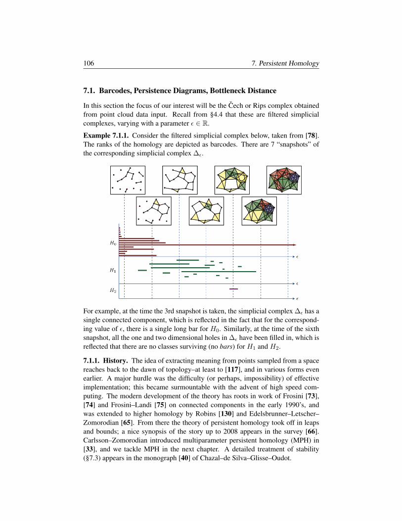
106 7. Persistent Homology
7.1. Barcodes, Persistence Diagrams, Bottleneck Distance
In this section the focus of our interest will be the Cech or Rips complex obtainedfrom point cloud data input. Recall from §4.4 that these are filtered simplicialcomplexes, varying with a parameter ε ∈ R.
Example 7.1.1. Consider the filtered simplicial complex below, taken from [78].The ranks of the homology are depicted as barcodes. There are 7 “snapshots” ofthe corresponding simplicial complex ∆ε.
For example, at the time the 3rd snapshot is taken, the simplicial complex ∆ε has asingle connected component, which is reflected in the fact that for the correspond-ing value of ε, there is a single long bar for H0. Similarly, at the time of the sixthsnapshot, all the one and two dimensional holes in ∆ε have been filled in, which isreflected that there are no classes surviving (no bars) for H1 and H2.
7.1.1. History. The idea of extracting meaning from points sampled from a spacereaches back to the dawn of topology–at least to [117], and in various forms evenearlier. A major hurdle was the difficulty (or perhaps, impossibility) of effectiveimplementation; this became surmountable with the advent of high speed com-puting. The modern development of the theory has roots in work of Frosini [73],[74] and Frosini–Landi [75] on connected components in the early 1990’s, andwas extended to higher homology by Robins [130] and Edelsbrunner–Letscher–Zomorodian [65]. From there the theory of persistent homology took off in leapsand bounds; a nice synopsis of the story up to 2008 appears in the survey [66].Carlsson–Zomorodian introduced multiparameter persistent homology (MPH) in[33], and we tackle MPH in the next chapter. A detailed treatment of stability(§7.3) appears in the monograph [40] of Chazal–de Silva–Glisse–Oudot.
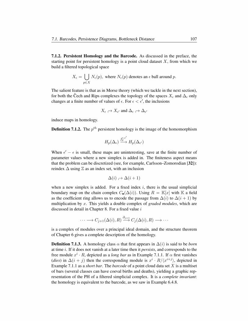
7.1. Barcodes, Persistence Diagrams, Bottleneck Distance 107
7.1.2. Persistent Homology and the Barcode. As discussed in the preface, thestarting point for persistent homology is a point cloud dataset X , from which webuild a filtered topological space
Xε =⋃p∈X
Nε(p), where Nε(p) denotes an ε ball around p.
The salient feature is that as in Morse theory (which we tackle in the next section),for both the Cech and Rips complexes the topology of the spaces Xε and ∆ε onlychanges at a finite number of values of ε. For ε < ε′, the inclusions
Xε → Xε′ and ∆ε → ∆ε′
induce maps in homology.
Definition 7.1.2. The pth persistent homology is the image of the homomorphism
Hp(∆ε)fε,ε′
p−→ Hp(∆ε′)
When ε′ − ε is small, these maps are uninteresting, save at the finite number ofparameter values where a new simplex is added in. The finiteness aspect meansthat the problem can be discretized (see, for example, Carlsson–Zomorodian [32]):reindex ∆ using Z as an index set, with an inclusion
∆(i) → ∆(i+ 1)
when a new simplex is added. For a fixed index i, there is the usual simplicialboundary map on the chain complex C•(∆(i)). Using R = K[x] with K a fieldas the coefficient ring allows us to encode the passage from ∆(i) to ∆(i + 1) bymultiplication by x. This yields a double complex of graded modules, which arediscussed in detail in Chapter 8. For a fixed value i
· · · −→ Cj+1(∆(i), R)∂j+1−→ Cj(∆(i), R) −→ · · ·
is a complex of modules over a principal ideal domain, and the structure theoremof Chapter 6 gives a complete description of the homology.
Definition 7.1.3. A homology class α that first appears in ∆(i) is said to be bornat time i. If it does not vanish at a later time then it persists, and corresponds to thefree module xi · R, depicted as a long bar as in Example 7.1.1. If α first vanishes(dies) in ∆(i + j) then the corresponding module is xi · R/〈xi+j〉, depicted inExample 7.1.1 as a short bar. The barcode of a point cloud data set X is a multisetof bars (several classes can have coeval births and deaths), yielding a graphic rep-resentation of the PH of a filtered simplicial complex. It is a complete invariant:the homology is equivalent to the barcode, as we saw in Example 6.4.8.
108 7. Persistent Homology
7.1.3. Computation of Persistent Homology. In [65], Edelsbrunner-Letscher-Zomorodian give an algorithm (often called the standard algorithm) for computingpersistent homology. Large data sets present considerable computational hurdles,and there have been many papers on extending or improving the algorithm. See forexample [32], [97], [105] and references therein, and [123] for an overview.
The main idea is to set up a pairing where birth-death (or birth) classes in homol-ogy have a distinguished representative. This echoes Morse theory, where criticalpoints carry a homological signal. The first step is to package all the boundarymaps ∂i into a single large matrix D. Let ∆(i) be the ith term in the filtration, andlet S be the set of all simplices (of all dimensions) appearing in the filtration, with|S| = n. We define n× n matrices D and R as follows:
(a) Linearly order S, such that σi ≺ σj for i ≤ j when either σi ⊆ σj orσj ⊆ ∆(j)\∆(i) and σi ∈ ∆(i) (so consistent with order of appearance).
(b) Dij = sgn(σi, σj) if σi is a codimension one face of σj , else Dij = 0.
(c) For j ∈ 1, . . . , n, define low(j) to be the largest row index of a nonzeroentry (i.e. the lowest or bottom-most) in column j; if column j containsall zeros, set low(j) = 0. A matrix is in reduced form if for every columnj having low(j) = i 6= 0, there is only one nonzero entry in row i.
(d) Do left to right column operations to transform D to a reduced matrix R.
The reduced matrix R encodes PH: if low(j) = i, and dim(σi) = m, then σisignals birth of a class in Hm, and σj the demise. If low(j) = 0 and j 6= low(k)for any k, then there is a birth at σj . An example is worth a thousand words:
Example 7.1.4. Consider the complex ∆ of Exercise 2.2.8, filtered as below
The order [1], [2], [12], [3], [13], [23], [123] satisfies (a) above, yielding
D =
0 0 1 0 1 0 00 0 −1 0 0 1 0
0 0 0 0 0 0 1
0 0 0 0 −1 −1 00 0 0 0 0 0 −1
0 0 0 0 0 0 1
0 0 0 0 0 0 0
and R =
0 0 1 0 1 0 00 0 −1 0 0 0 0
0 0 0 0 0 0 1
0 0 0 0 −1 0 00 0 0 0 0 0 −1
0 0 0 0 0 0 1
0 0 0 0 0 0 0
We obtain classes in PH as below. The class corresponding to [1] is persistent.
low([12]) = [2]. [2] born at time 1, dies at time 1 → no class.low([13]) = [3]. [3] born at time 2, dies at time 3 → class in H0.low([123]) = [23]. [23] born at time 3, dies at time 4 → class in H1.low([1]) = 0. [1] born at time 0, 6 ∃k | low(k) = [1] → class in H0.
7.1. Barcodes, Persistence Diagrams, Bottleneck Distance 109
7.1.4. Alpha and Witness complexes. As noted in Chapter 4, the Cech complexrequires determination of the intersections between neighborhoods of points, whichcan be computationally intensive. A first analysis of the runtime for the reductionalgorithm in the previous section might indicate that it has complexity O(n3), but[112] shows this can be improved to O(n2.376).
One way to improve runtime is to construct variants of the Cech complex whichinvolve a smaller number of simplices. Below we give a quick overview of twoother commonly used complexes, the Alpha complex introduced by Edelsbrunner-Kirkpatrick-Seidel in [64] and the Witness complex introduced by de Silva–Carlssonin [51]. To describe the Alpha complex, we need to define Voronoi cells:
Definition 7.1.5. For a finite point set X ⊆ Rd, the Voronoi cell of x ∈ X is
V (x) = p ∈ Rn such that ||x− p|| ≤ ||y − p|| for all y ∈ X
For a parameter δ, the Alpha complex Aδ(X) is the nerve (as in Definition 4.1.5)of the cover consisting of the union of the sets Nδ(x) ∩ V (x).
When δ →∞, the intersections Nδ(x)∩V (x) are just the Voronoi cells; the nerveof the resulting cover is the Delaunay complex. The Delaunay complex does nottypically have a geometric realization, but a notable exception occurs when thepoints of X are sufficiently general (not too many points on a linear subspace orsphere), in which case the resulting geometric realization is a triangulation of theconvex hull of X . The initial motivation came from the setting X ⊆ R2, whereusing the Alpha complex results in a substantial speed up (coming from duality).See [66] for a detailed discussion.
For the Witness complex, the key idea is to identify distinguished subsets of a finiteset X that encode the key features of the set.
Definition 7.1.6. Let Y ⊆ X ⊆ Rd with X finite. A point p ∈ Rd is a weakwitness at scale ε for Y with respect to X if ||p − y|| ≤ ||p − x|| + ε for ally ∈ Y , x ∈ X \ Y . The witness complex D(X, ε) has a vertex for each x ∈ X;[xi0 , . . . , xik ] is a k-simplex of D(X, ε) exactly if it has a weak witness at scale ε.
A point p ∈ S is a weak witness for a subset Y of X when p is a sort of “cen-ter of attraction” or “landmark” for the points of Y , while the points of X \ Yremain standoffish (at a further distance from p than the points of Y ). Thus, incertain circumstances, the cluster of points forming Y may represent a simplex ofdimension ≤ |Y | − 1 in our original sample, so the set Y is in some sense beingrepresented by the single point p. The papers of Attali–Edelsbrunner–Mileyko [5]and Guibas–Oudot [85] give conditions under which witness complexes can dis-cern the topology of curves and surfaces in Rd. Both the Alpha complex and theWitness complex can be generalized to other metric spaces.
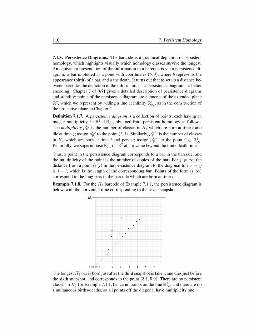
110 7. Persistent Homology
7.1.5. Persistence Diagrams. The barcode is a graphical depiction of persistenthomology, which highlights visually which homology classes survive the longest.An equivalent presentation of the information in a barcode is via a persistence di-agram: a bar is plotted as a point with coordinates (b, d), where b represents theappearance (birth) of a bar, and d the death. It turns out that to set up a distance be-tween barcodes the depiction of the information as a persistence diagram is a betterencoding. Chapter 7 of [67] gives a detailed description of persistence diagramsand stability; points of the persistence diagram are elements of the extended planeR2, which we represent by adding a line at infinity R1
∞, as in the construction ofthe projective plane in Chapter 2.
Definition 7.1.7. A persistence diagram is a collection of points, each having aninteger multiplicity, in R2 ∪ R1
∞, obtained from persistent homology as follows.The multiplicity µi,jp is the number of classes in Hp which are born at time i anddie at time j; assign µi,jp to the point (i, j). Similarly, µi,∞p is the number of classesin Hp which are born at time i and persist; assign µi,∞p to the point i ∈ R1
∞.Pictorially, we superimpose R1
∞ on R2 at a y value beyond the finite death times.
Thus, a point in the persistence diagram corresponds to a bar in the barcode, andthe multiplicity of the point is the number of copies of the bar. For j 6= ∞, thedistance from a point (i, j) in the persistence diagram to the diagonal line x = yis j − i, which is the length of the corresponding bar. Points of the form (i,∞)correspond to the long bars in the barcode which are born at time i.
Example 7.1.8. For the H1 barcode of Example 7.1.1, the persistence diagram isbelow, with the horizontal time corresponding to the seven snapshots.
21 3 4 5 6 7Snapshot
The longestH1 bar is born just after the third snapshot is taken, and dies just beforethe sixth snapshot, and corresponds to the point (3.1, 5.9). There are no persistentclasses in H1 for Example 7.1.1, hence no points on the line R1
∞, and there are nosimultaneous births/deaths, so all points off the diagonal have multiplicity one.
7.1. Barcodes, Persistence Diagrams, Bottleneck Distance 111
7.1.6. Metrics on diagrams. For persistent homology to be useful, if two datasets X and Y are “close”, then their persistence diagrams should be close. So ourfirst task is to define a metric on persistence diagrams. The Hausdorff metric is astandard way to make the set of compact subsets of a metric space into a metricspace itself.
Definition 7.1.9. Let X and Y be two non-empty subsets of a metric space withmetric d. The Hausdorff distance between X and Y is
dH(X,Y ) = maxsupx∈X
infy∈Y
d(x, y), supy∈Y
infx∈X
d(x, y)
Put simply, the Hausdorff distance is the longest distance between a point x ∈ Xand the point in Y closest to x.
To define a distance between sets X and Y corresponding to persistence diagrams,we take Hausdorff distance as a starting point. This entails setting up a matchingbetween the points of X and the points of Y, in such a way that the biggest (thinkworst) distance between a pair is minimized. However, by its nature, data is oftennoisy or incomplete. So we instead work with
Definition 7.1.10. A partial matching µ between two finite sets X and Y is abijection between two subsets X ′ ⊆ X and Y ′ ⊆ Y . We call X ′ the coimage of µ,and Y ′ the image of µ.
In the setting of persistence diagrams, X and Y will be finite sets of points(with multiplicity–we could have two classes in homology born and dying at thesame time) in R2. But again, we have a roadblock–what shall we do with theleftovers–those points not included in the matching? The solution turns out to beadding in the diagonal, in a way we make precise below. First, recall that the `∞distance between two points p = (p1, p2) and q = (q1, q2) is
(7.1.1) ||p− q||∞ = max|p1 − q1|, |p2 − q2|.The distance between two persistence diagrams is defined by first finding the costof a partial matching, and then minimizing the cost over all partial matchings:
Definition 7.1.11. The cost of a partial match µ between X ′ ⊆ X and Y ′ ⊆ Y is
(7.1.2)
c(µ) = max supp′∈X′
||p′ − µ(p′)||∞,
supp∈X\X′
p2−p1
2 ,
supq∈Y \Y ′
q2−q12
The bottleneck distance between two persistence diagrams X and Y is
(7.1.3) dB(X,Y ) = minc(µ) | µ a partial matchingExercise 7.1.12. Show that for p = (p1, p2) ∈ R2, the quantity p2−p1
2 is thedistance from p to the diagonal x = y.

112 7. Persistent Homology
Example 7.1.13. To understand what this means in practice, consider the persis-tence diagrams X = p1,p2,p3,p4 and Y = q1,q2,q3,q4 below
(a) For the empty partial match µ0 where no points are matched, the cost issimply the max of the distances of the points (in both X and Y ) to thediagonal, so c(µ0) = 5.
(b) For the partial match µ1 = pi 7→ q5−i, the cost is maximized at thedistance between p1 and q4, so c(µ1) = 8.
(c) For the partial match µ2 = pi 7→ qi, the distances are all 2, so c(µ2) = 2.
It is easy to verify that in fact µ2 minimizes the cost, hence dB(X,Y ) = 2.
This is all well and good, but we have not even verified that dB is a metric.Before doing this, we ask “Where does the name “bottleneck” come from?” Thenext exercise will answer this.
Exercise 7.1.14. We consider sets of four points as in the previous example. Theset X is unchanged, but in the set Y , the points q2,q3,q4 have changed posi-tion.
Compute dB(X,Y ). Where does the name “bottleneck” come from?
7.1. Barcodes, Persistence Diagrams, Bottleneck Distance 113
Theorem 7.1.15. The bottleneck distance dB is a metric on persistence diagrams.
Proof. It follows from the definition that dB(X,X) = 0 and
dB(X,Y ) = dB(Y,X),
so the interesting part is the triangle inequality: we need to show that for threepersistence diagrams X,Y, Z that
(7.1.4) dB(X,Z) ≤ dB(X,Y ) + dB(Y, Z).
First, note that adding the diagonal to every persistence diagram means in partic-ular that an unmatched point p = (p1, p2) ∈ X can be matched to a point of thediagonal of Y , and the distance is p2−p1
2 . This means that the three different sub-sets which need be considered in the computation of the cost of a partial match µbetween X and Y as in Equation 7.1.2 may be consolidated into the single condi-tion
c(µ) = maxsupp∈X||p− µ(p)||∞,
Now let µ1, µ2, and µ3 be matchings that minimize the respective cost functions,so that
dB(X,Z) = c(µ1)dB(X,Y ) = c(µ2)dB(Y, Z) = c(µ3)
Now observe that we can compose partial matches: Suppose µXY is a partial matchfrom X −→ Y and µY Z is a partial match from Y −→ Z. Composing the twogives a partial match µXZ . Note that this can be the empty match, if the target Y ′
of µXY is disjoint from the source of µY Z . Hence
dB(X,Z) = c(µ1)= maxsup
p∈X||p− µ1(p)||∞
≤ maxsupp∈X||p− µ3µ2(p)||∞
≤ maxsupp∈X||p− µ2(p)||∞ = c(µ2)
+ maxsupq∈Y||q− µ3(q)||∞ = c(µ3)
= dB(X,Y ) + dB(Y,Z)
In going from row 3 to row 4 in the argument, we are using the triangle inequalityon the individual points
||p− µ3µ2(p)||∞ ≤ ||p− µ2(p)||∞ + ||µ2(p)− µ3µ2(p)||∞What about long bars and the corresponding points on R1
∞? Because we are deal-ing with a finite data set, by taking ε 0, all homology classes will have died,save a single component in H0, which allows us to deal with this situation.
114 7. Persistent Homology
7.2. Morse Theory
Persistent homology is similar to Morse theory, and to understand persistent ho-mology it will be useful to have Morse theory as a backdrop. Morse developed themachinery almost a century ago in [115], [116]. We give a brief overview here inthe spirit of [20] or [150]; for a more comprehensive treatment, see [108] or [111].
Definition 7.2.1. A smooth function Mf→ R on an n-dimensional compact man-
ifold is defined on open sets U ⊆ M having local coordinates x1, . . . , xn. Thefunction f is Morse if it has a finite number of critical points: those p where
∂f
∂x1(p) = · · · = ∂f
∂xn(p) = 0,
and the critical points are distinct and nondegenerate: the determinant of the Hes-sian matrix
Hf =
∂2f∂x2
1(p) · · · ∂2f
∂x1∂xn(p)
.... . .
...∂2f
∂xn∂x1(p) · · · ∂2f
∂x2n
(p)
is nonzero at critical points. Morse theory generalizes the second derivative test.
Example 7.2.2. Flashback to vector calculus: the graph of z = f(x, y) defines asurface S in R3. The critical points of f are the points p where
∂f
∂x(p) = 0 =
∂f
∂y(p),
so the tangent plane Tp(S) is horizontal and p is a max, min, or saddle point.
Exercise 7.2.3. Find the critical points and Hessians for the following functions
z = x2 + y2, z = x2 − y2, z = −x2 − y2.
Determine if the critical point is a max, min, or saddle. A key ingredient in Morse Theory is the Morse Lemma:
Lemma 7.2.4. For a Morse function f , if p is a critical point, then there exists acoordinate system x1, . . . , xn so that
f(x1, . . . , xn) = f(p)−λp∑i=1
x2i +
n∑j=λp+1
x2j
It follows immediately from the Morse Lemma that at a critical point p, the Hessianmatrix is diagonal, with λp entries of −2, and n − λp entries of +2. This meansthat λp is the number of negative eigenvalues of the Hessian at a critical point p.
Definition 7.2.5. The sublevel sets of a function f on M are Mr = f−1(−∞, r].
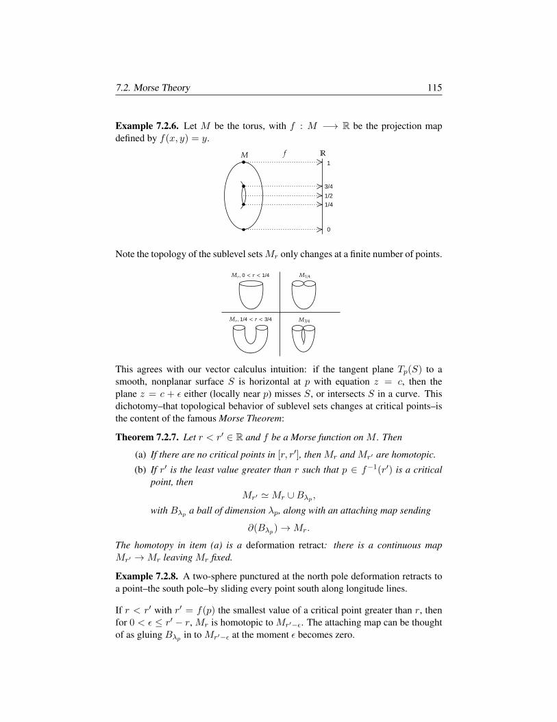
7.2. Morse Theory 115
Example 7.2.6. Let M be the torus, with f : M −→ R be the projection mapdefined by f(x, y) = y.
1/4
0
1/2
3/4
1
Note the topology of the sublevel setsMr only changes at a finite number of points.
, 0 1/4
, 1/4 3/4
This agrees with our vector calculus intuition: if the tangent plane Tp(S) to asmooth, nonplanar surface S is horizontal at p with equation z = c, then theplane z = c + ε either (locally near p) misses S, or intersects S in a curve. Thisdichotomy–that topological behavior of sublevel sets changes at critical points–isthe content of the famous Morse Theorem:
Theorem 7.2.7. Let r < r′ ∈ R and f be a Morse function on M . Then
(a) If there are no critical points in [r, r′], then Mr and Mr′ are homotopic.
(b) If r′ is the least value greater than r such that p ∈ f−1(r′) is a criticalpoint, then
Mr′ 'Mr ∪Bλp ,with Bλp a ball of dimension λp, along with an attaching map sending
∂(Bλp)→Mr.
The homotopy in item (a) is a deformation retract: there is a continuous mapMr′ →Mr leaving Mr fixed.
Example 7.2.8. A two-sphere punctured at the north pole deformation retracts toa point–the south pole–by sliding every point south along longitude lines.
If r < r′ with r′ = f(p) the smallest value of a critical point greater than r, thenfor 0 < ε ≤ r′ − r, Mr is homotopic to Mr′−ε. The attaching map can be thoughtof as gluing Bλp in to Mr′−ε at the moment ε becomes zero.
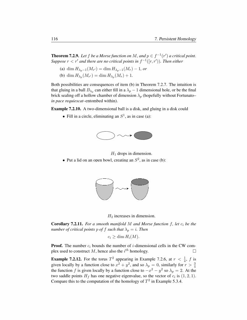
116 7. Persistent Homology
Theorem 7.2.9. Let f be a Morse function onM , and p ∈ f−1(r′) a critical point.Suppose r < r′ and there are no critical points in f−1([r, r′)). Then either
(a) dimHλp−1(Mr′) = dimHλp−1(Mr)− 1, or
(b) dimHλp(Mr′) = dimHλp(Mr) + 1.
Both possibilities are consequences of item (b) in Theorem 7.2.7. The intuition isthat gluing in a ball Bλp can either fill in a λp − 1 dimensional hole, or be the finalbrick sealing off a hollow chamber of dimension λp (hopefully without Fortunato–in pace requiescat–entombed within).
Example 7.2.10. A two-dimensional ball is a disk, and gluing in a disk could
• Fill in a circle, eliminating an S1, as in case (a):
H1 drops in dimension.
• Put a lid on an open bowl, creating an S2, as in case (b):
H2 increases in dimension.
Corollary 7.2.11. For a smooth manifold M and Morse function f , let ci be thenumber of critical points p of f such that λp = i. Then
ci ≥ dimHi(M).
Proof. The number ci bounds the number of i-dimensional cells in the CW com-plex used to construct M , hence also the ith homology.
Example 7.2.12. For the torus T 2 appearing in Example 7.2.6, at r < 14 , f is
given locally by a function close to x2 + y2, and so λp = 0, similarly for r > 34
the function f is given locally by a function close to −x2 − y2 so λp = 2. At thetwo saddle points Hf has one negative eigenvalue, so the vector of ci is (1, 2, 1).Compare this to the computation of the homology of T 2 in Example 5.3.4.
7.3. The Stability Theorem 117
Definition 7.2.13. A continuous real valued function f on a space X has a homo-logical critical value at q if the map induced by inclusion
limε→0
[Hp(f
−1(−∞, q − ε))→ Hp(f−1(−∞, q + ε))
]is not an isomorphism. The function f is tame if it has a finite number of homo-logical critical values, and the homology Hp(f
−1(−∞, q],K) of the sublevel setsis finite dimensional for all points q ∈ X .
For example, ifX is smooth and f is a Morse function then the homological criticalpoints are the usual critical points of f . Tame functions are the right setting for themain result of the next section.
7.3. The Stability Theorem
For a manifold M and smooth real valued function f : M → R, the sublevelsets Mr = f−1(−∞, r] appearing in §2 yield a filtration of M . In this section,we outline work of Cohen-Steiner–Edelsbrunner–Harer [44], which proves a sta-bility theorem for persistent homology; [57] calls their result “arguably the mostpowerful theorem in TDA”. The motivation is natural: for persistent homology tobe useful, if two spaces X and Y are close, then their corresponding persistencediagrams should also be close. Recall that
Definition 7.3.1. For functions f, g : X → R, the sup or L∞ norm is
‖f − g‖∞ = maxx∈X|f(x)− g(x)|.
Let f : X → R and letD(f) be the persistence diagram of some homology moduleof the filtration on X induced by f . The main theorem of [44] is
Theorem 7.3.2. [Stability Theorem] Let X be a triangulable space and f, g con-tinuous tame real valued functions on X . Then the persistence diagrams of f andg satisfy dB(D(f), D(g)) ≤ ||f − g||∞.
To tackle stability, we proceed as follows: first, suppose that X is a manifold andf, g are Morse functions. By Theorem 7.2.9 of the previous section, there are afinite number of critical points, and in this context the main result on stability is thestatement that the bottleneck distance between the persistence diagrams of f and gis bounded by the L∞ distance between the functions f and g themselves.
The proof by Cohen-Steiner–Edelsbrunner–Harer in [44] involves a fairly intri-cate diagram chase. We instead give the proof due to Cohen-Steiner–Edelsbrunner–Morozov [46] of a slightly weaker version: Theorem 7.3.7 below applies in thesetting of simplicial complexes and monotone functions, so it is well suited to han-dle the Cech or Rips complex arising from point cloud data. Before moving to theformal proof, we sketch an intuitive example
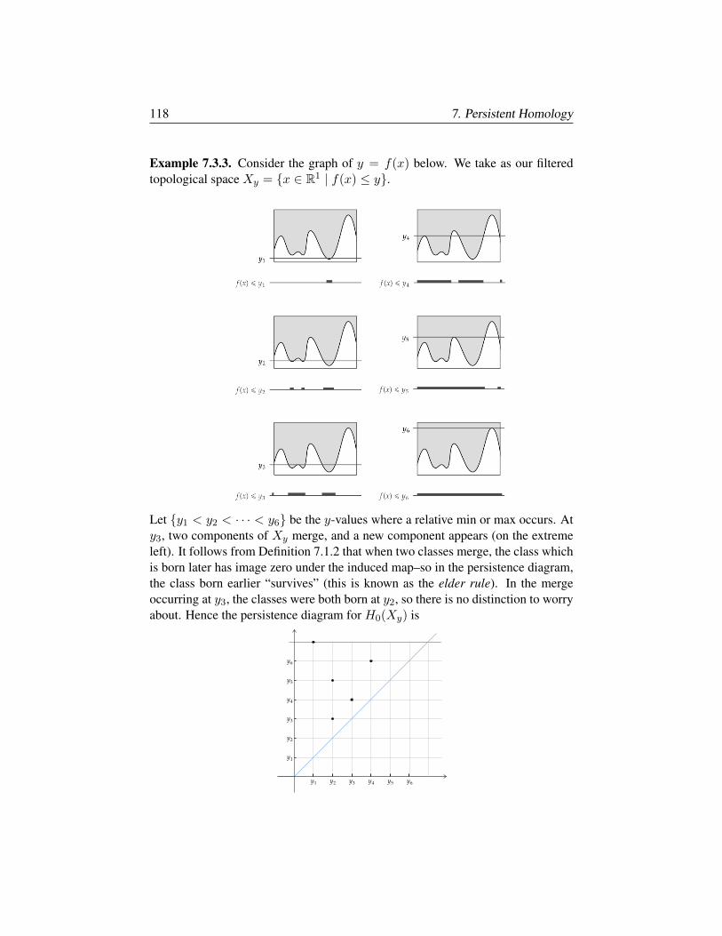
118 7. Persistent Homology
Example 7.3.3. Consider the graph of y = f(x) below. We take as our filteredtopological space Xy = x ∈ R1 | f(x) ≤ y.
Let y1 < y2 < · · · < y6 be the y-values where a relative min or max occurs. Aty3, two components of Xy merge, and a new component appears (on the extremeleft). It follows from Definition 7.1.2 that when two classes merge, the class whichis born later has image zero under the induced map–so in the persistence diagram,the class born earlier “survives” (this is known as the elder rule). In the mergeoccurring at y3, the classes were both born at y2, so there is no distinction to worryabout. Hence the persistence diagram for H0(Xy) is
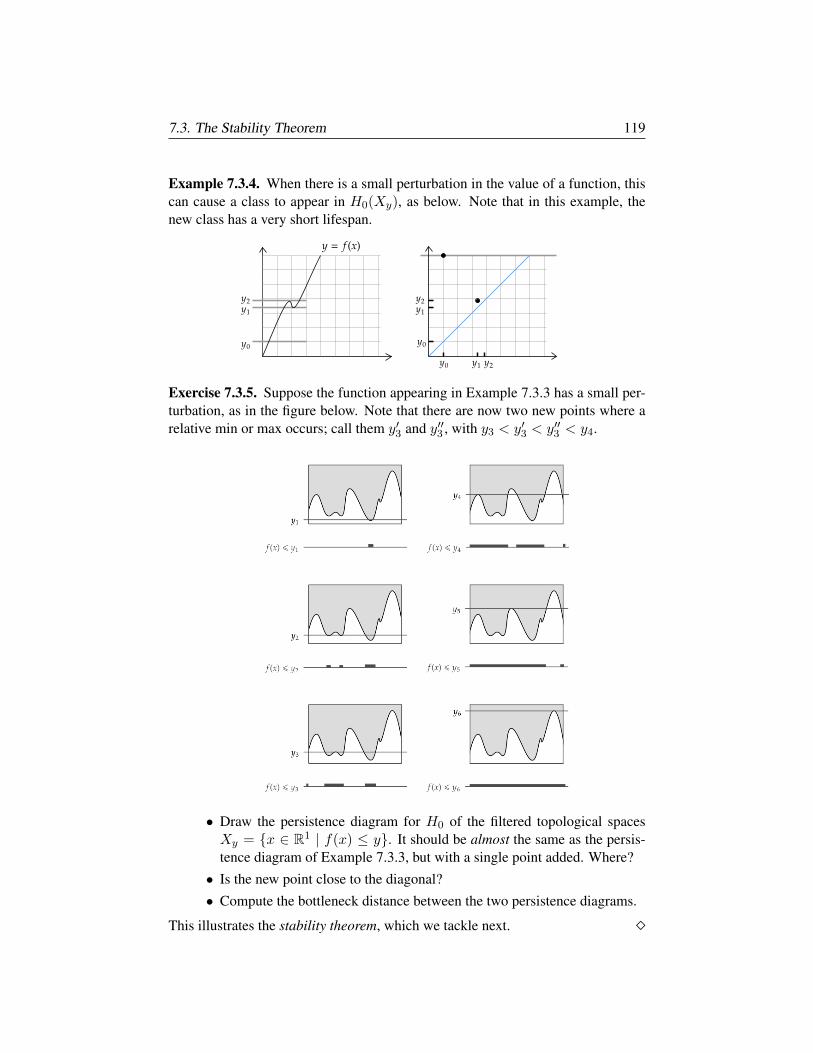
7.3. The Stability Theorem 119
Example 7.3.4. When there is a small perturbation in the value of a function, thiscan cause a class to appear in H0(Xy), as below. Note that in this example, thenew class has a very short lifespan.
Exercise 7.3.5. Suppose the function appearing in Example 7.3.3 has a small per-turbation, as in the figure below. Note that there are now two new points where arelative min or max occurs; call them y′3 and y′′3 , with y3 < y′3 < y′′3 < y4.
• Draw the persistence diagram for H0 of the filtered topological spacesXy = x ∈ R1 | f(x) ≤ y. It should be almost the same as the persis-tence diagram of Example 7.3.3, but with a single point added. Where?
• Is the new point close to the diagonal?
• Compute the bottleneck distance between the two persistence diagrams.
This illustrates the stability theorem, which we tackle next.
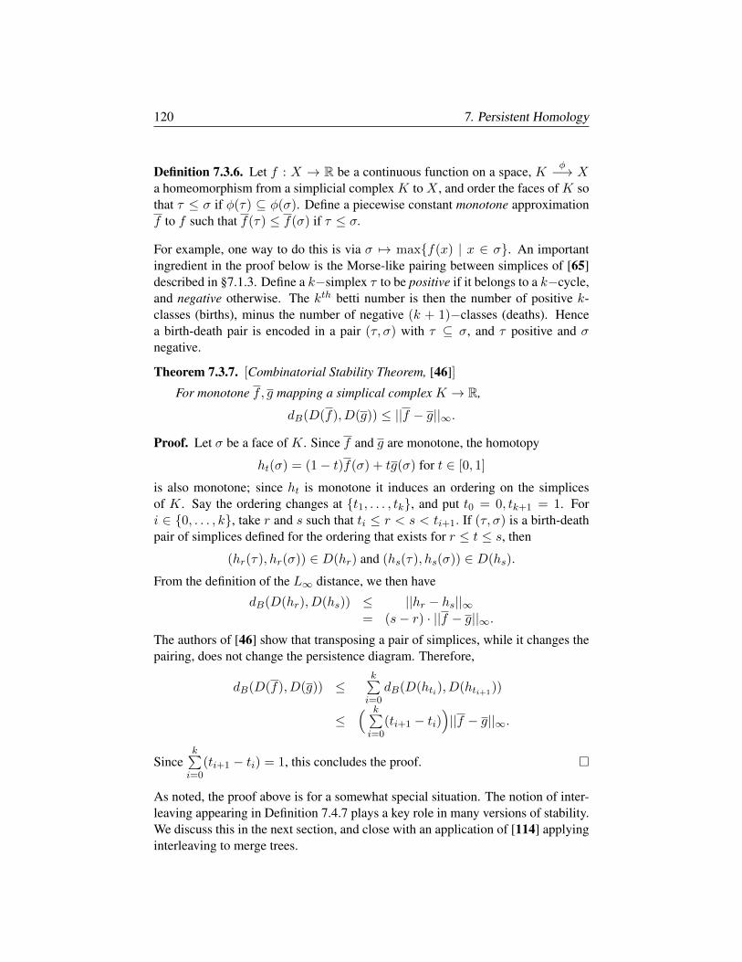
120 7. Persistent Homology
Definition 7.3.6. Let f : X → R be a continuous function on a space, Kφ−→ X
a homeomorphism from a simplicial complex K to X , and order the faces of K sothat τ ≤ σ if φ(τ) ⊆ φ(σ). Define a piecewise constant monotone approximationf to f such that f(τ) ≤ f(σ) if τ ≤ σ.
For example, one way to do this is via σ 7→ maxf(x) | x ∈ σ. An importantingredient in the proof below is the Morse-like pairing between simplices of [65]described in §7.1.3. Define a k−simplex τ to be positive if it belongs to a k−cycle,and negative otherwise. The kth betti number is then the number of positive k-classes (births), minus the number of negative (k + 1)−classes (deaths). Hencea birth-death pair is encoded in a pair (τ, σ) with τ ⊆ σ, and τ positive and σnegative.
Theorem 7.3.7. [Combinatorial Stability Theorem, [46]]
For monotone f, g mapping a simplical complex K → R,
dB(D(f), D(g)) ≤ ||f − g||∞.
Proof. Let σ be a face of K. Since f and g are monotone, the homotopy
ht(σ) = (1− t)f(σ) + tg(σ) for t ∈ [0, 1]
is also monotone; since ht is monotone it induces an ordering on the simplicesof K. Say the ordering changes at t1, . . . , tk, and put t0 = 0, tk+1 = 1. Fori ∈ 0, . . . , k, take r and s such that ti ≤ r < s < ti+1. If (τ, σ) is a birth-deathpair of simplices defined for the ordering that exists for r ≤ t ≤ s, then
(hr(τ), hr(σ)) ∈ D(hr) and (hs(τ), hs(σ)) ∈ D(hs).
From the definition of the L∞ distance, we then have
dB(D(hr), D(hs)) ≤ ||hr − hs||∞= (s− r) · ||f − g||∞.
The authors of [46] show that transposing a pair of simplices, while it changes thepairing, does not change the persistence diagram. Therefore,
dB(D(f), D(g)) ≤k∑i=0
dB(D(hti), D(hti+1))
≤( k∑i=0
(ti+1 − ti))||f − g||∞.
Sincek∑i=0
(ti+1 − ti) = 1, this concludes the proof.
As noted, the proof above is for a somewhat special situation. The notion of inter-leaving appearing in Definition 7.4.7 plays a key role in many versions of stability.We discuss this in the next section, and close with an application of [114] applyinginterleaving to merge trees.
7.4. Interleaving and Categories 121
7.4. Interleaving and Categories
Persistent Homology fits naturally into a category theoretic framework, and thisviewpoint will be useful in formulating the concept of interleaving distance. Thereason to bring interleaving distance into the picture is that it provides a naturalway to define a metric on spaces related to diagrams.
7.4.1. Categories and Functors. Category Theory is an abstract framework thatencompasses homology, persistent homology, and constructions such as Hom, ⊗,and localization. Used judiciously, category theory provides a powerful tool tostreamline and unify many mathematical constructions, see MacLane [107] orRiehl [128] for detailed expositions.
In this section we’ll see that persistent homology can be regarded as a functorfrom the poset category of the real numbers (R,≤) to the category of vector spacesover a chosen field K. We begin by giving a brief review of categories and functors;the material is developed in depth when we introduce derived functors in Chapter9. Then we define the interleaving distance, and show that it does define a metric.For a detailed exposition on interleaving and stability, see the monograph [40] byChazal–de Silva–Glisse–Oudot.
Definition 7.4.1. A Category A consists of
• A collection of objects Ob(A ).
• A collection of morphisms: for A,B ∈ Ob(A ), a set Hom(A,B),
such that morphisms can be composed. The composition is associative, and foreach object A, there is an identity morphism 1A : A→ A.
Example 7.4.2. Examples of categories
• Set: Sets and functions.
• P: Posets and order preserving functions.
• Vect: Vector spaces and linear transformations.
• Top: Topological spaces and continuous maps.
In many mathematical settings we deal with objects and maps between them. Amap between categories is
Definition 7.4.3. A functor F is a function from a category A to a category B,which takes objects to objects Ob(A )
F⇒ Ob(B) and morphisms to morphisms ina way that preserves identities and compositions. The functor F is covariant if
F : Af→ A′ ∈ Hom(A,A′) =⇒ F (A)
F (f)→ F (A′) ∈ Hom(F (A), F (A′)),
and contravariant if
F : Af→ A′ ∈ Hom(A,A′) =⇒ F (A′)
F (f)→ F (A) ∈ Hom(F (A′), F (A)).
122 7. Persistent Homology
Exercise 7.4.4. For a commutative ring R, show the set of R-modules and R-module homomorphisms is a category R-mod, and for a fixed module N , that
(a) HomR(N, •) is covariant, and HomR(•, N) is contravariant.
(b) • ⊗R (N) is covariant.
What happens when composing functors? The functors above take R-mod to R-mod. Functors are most interesting when theyprovide a way to translate between categories that are of very different flavors.
Example 7.4.5. Homology is a functor for any of the homology theories of Chap-ters 4 and 5; for example, singular homology takes Top to Vect:
• if X 1X−→ X then Hi(X)H(1X)−→ Hi(X).
• if Xf−→ Y and if Y
g−→ Z then Hi(g f) = Hi(g) Hi(f).
Exercise 7.4.6. Connect the two concepts below using category theory.
(a) In Definition 3.1.9, we defined a homotopy of maps: two continuous mapsof topological spaces f0, f1 : S → T are homotopic if there is a continu-ous map F such that
S × [0, 1]F−→ T
with F (x, 0) = f0(x) and F (x, 1) = f1(x); F deforms f0 to the map f1.
(b) In Definition 4.3.7, we defined a chain homotopy of complexes: givenchain maps
Aiαi−→ Bi and Ai
βi−→ Bi
a chain homotopy is a map
Aiγi−→ Bi+1
such thatαi − βi = γi−1δi + ∂i+1γi
in the diagram below
// Ai+1δi+1 // Ai
αi−βi
δi //
γi
Ai−1
γi−1
//
// Bi+1∂i+1 // Bi
∂i // Bi−1//
Theorem 4.3.8 shows that chain homotopic maps induce the same map on homol-ogy. Prove that homotopic maps of type (a) induce homotopic maps of type (b),and show Theorem 4.2.11 follows as a corollary.
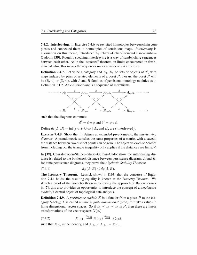
7.4. Interleaving and Categories 123
7.4.2. Interleaving. In Exercise 7.4.6 we revisited homotopies between chain com-plexes and connected them to homotopies of continuous maps. Interleaving isa variation on this theme, introduced by Chazal–Cohen-Steiner–Glisse–Guibas–Oudot in [39]. Roughly speaking, interleaving is a way of sandwiching sequencesbetween each other. As in the “squeeze” theorem on limits encountered in fresh-man calculus, this means the sequences under consideration are close.
Definition 7.4.7. Let C be a category and A•, B• be sets of objects of C , withmaps indexed by pairs of related elements of a poset P . For us, the poset P willbe (R,≤) or (Z,≤), with A and B families of persistent homology modules as inDefinition 7.1.2. An ε-interleaving is a sequence of morphisms
// Atd //
ψ
!!
At+εd //
ψ
""
At+2εd //
ψ
##
At+3ε//
// Btδ //
φ
==
Bt+εδ //
φ
<<
Bt+2εδ //
φ
;;
Bt+3ε//
such that the diagrams commute:
d2 = ψ φ and δ2 = φ ψ.Define dI(A,B) = infε ∈ P ∪∞ | A• and B• are ε-interleaved.Exercise 7.4.8. Show that dI defines an extended pseudometric, the interleavingdistance. A pseudometric satisfies the same properties of a metric, with a caveat:the distance between two distinct points can be zero. The adjective extended comesfrom including∞; the triangle inequality only applies if the distances are finite. In [39], Chazal–Cohen-Steiner–Glisse–Guibas–Oudot show the interleaving dis-tance is related to the bottleneck distance between persistence diagrams A and B:for tame persistence diagrams, they prove the Algebraic Stability Theorem:
(7.4.1) dB(A,B) ≤ dI(A,B).
The Isometry Theorem. Lesnick shows in [103] that the converse of Equa-tion 7.4.1 holds; the resulting equality is known as the Isometry Theorem. Wesketch a proof of the isometry theorem following the approach of Bauer-Lesnickin [7]; this also provides an opportunity to introduce the concept of a persistencemodule, a central object of topological data analysis.
Definition 7.4.9. A persistence module X is a functor from a poset P to the cat-egory VectK; X is called pointwise finite dimensional (p.f.d) if it takes values infinite dimensional vector spaces. So if x1 x2 x3 in P , then there are lineartransformations of the vector spaces X(xi)
(7.4.2) X(x1)X21−→ X(x2)
X32−→ X(x3),
such that Xii is the identity, and X32 X21 = X31 .
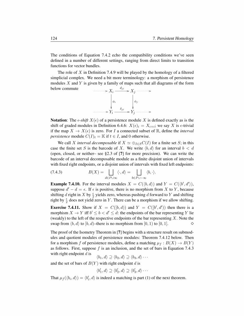
124 7. Persistent Homology
The conditions of Equation 7.4.2 echo the compatibility conditions we’ve seendefined in a number of different settings, ranging from direct limits to transitionfunctions for vector bundles.
The role of X in Definition 7.4.9 will be played by the homology of a filteredsimplicial complex. We need a bit more terminology: a morphism of persistencemodules X and Y is given by a family of maps such that all diagrams of the formbelow commute // Xi
dji //
φi
Xj
φj
//
// Yiδji // Yj //
Notation: The ε-shift X(ε) of a persistence module X is defined exactly as is theshift of graded modules in Definition 6.4.6: X(ε)i = Xε+i; we say X is ε-trivialif the map X → X(ε) is zero. For I a connected subset of R, define the intervalpersistence module C(I)t = K if t ∈ I , and 0 otherwise.
We call X interval decomposable if X ' ⊕I∈SC(I) for a finite set S; in thiscase the finite set S is the barcode of X . We write 〈b, d〉 for an interval b < d(open, closed, or neither– see §2.3 of [7] for more precision). We can write thebarcode of an interval decomposable module as a finite disjoint union of intervalswith fixed right endpoints, or a disjoint union of intervals with fixed left endpoints:
(7.4.3) B(X) =⊔
d∈P∪∞〈·, d〉 =
⊔b∈P∪−∞
〈b, ·〉.
Example 7.4.10. For the interval modules X = C(〈b, d〉) and Y = C(〈b′, d′〉),suppose d′ − d = ε. If ε is positive, there is no morphism from X to Y , becauseshifting d right inX by ε
2 yields zero, whereas pushing d forward to Y and shiftingright by ε
2 does not yield zero in Y . There can be a morphism if we allow shifting.
Exercise 7.4.11. Show if X = C([b, d)) and Y = C([b′, d′)) then there is amorphism X → Y iff b′ ≤ b < d′ ≤ d: the endpoints of the bar representing Y lie(weakly) to the left of the respective endpoints of the bar representing X . Note theswap from 〈b, d〉 to [b, d)–there is no morphism from [0, 1) to [0, 1]. The proof of the Isometry Theorem in [7] begins with a structure result on submod-ules and quotient modules of persistence modules: Theorem 7.4.12 below. Thenfor a morphism f of persistence modules, define a matching µf : B(X) → B(Y )as follows. First, suppose f is an inclusion, and the set of bars in Equation 7.4.3with right endpoint d is
〈b1, d〉 ⊇ 〈b2, d〉 ⊇ 〈b3, d〉 · · ·and the set of bars of B(Y ) with right endpoint d is
〈b′1, d〉 ⊇ 〈b′2, d〉 ⊇ 〈b′3, d〉 · · ·That µf (〈bi, d〉) = 〈b′i, d〉 is indeed a matching is part (1) of the next theorem.
7.4. Interleaving and Categories 125
Theorem 7.4.12. [[7], Theorem 4.2] For p.f.d. persistence modules X and Y , ifthere is an injection φ : X → Y , then for a fixed d,
(1) : |〈·, d〉 ⊆ B(X)| ≤ |〈·, d〉 ⊆ B(Y )|.
If there is a surjection φ : X Y then for a fixed b,
(2) : |〈b, ·〉 ⊆ B(X)| ≥ |〈b, ·〉 ⊆ B(Y )|.
(1) yields a map B(X) → B(Y ) via 〈bi, d〉 7→ 〈b′i, d〉 for i ≤ |〈·, d〉 ⊆ B(X)|.(2) yields a map B(Y ) → B(X) via 〈b, d′i〉 7→ 〈b, di〉 for i ≤ |〈b, ·〉 ⊆ B(Y )|.
Definition 7.4.13. A matching of barcodes µ is called an ε-matching if(a) B(X)2ε ⊆ coim(µ) and B(Y )2ε ⊆ im(µ).(b) If µ(〈b, d〉) = 〈b′, d′〉, then 〈b, d〉 ⊆ 〈b′− ε, d′+ ε〉 and 〈b′, d′〉 ⊆ 〈b− ε, d+ ε〉.
So dB(B(X), B(Y )) = infε | ∃ an ε − matching between B(X) and B(Y ).Our aim is to produce an ε-matching from an ε-interleaving. Let B(Z)γ denote thebars of B(Z) of length ≥ γ, and let coim(µ), im(µ) be as in Definition 7.1.10.
Theorem 7.4.14. [Induced Matching,[7], Theorem 6.1]For a map of p.f.d. modules f : X → Y , suppose µf (〈b, d〉) = 〈b′, d′〉, then
• If coker(f) is ε-trivial, then all intervals of length ≥ ε in B(Y ) are con-tained in im(µf ) and b′ ≤ b ≤ b′ + ε.
• If ker(f) is ε-trivial, then all intervals of length ≥ ε in B(X) are con-tained in coim(µf ) and d− ε ≤ d′ ≤ d.
An interleaving of persistence modules f : X −→ Y (indeed, any map) factors as
(7.4.4) X im(f) → Y.
The proof of the Isometry Theorem hinges on using this factorization to matchB(im(f)) with both B(X) and B(Y ). The next example (5.2 of [7]) illustratesthat the induced matching obtained from the factorization is somewhat subtle.
Example 7.4.15. Let X = C(〈1, 2〉)⊕C(〈1, 3〉) and Y = C(〈0, 2〉)⊕C(〈3, 4〉),with f : X → Y injecting C(〈1, 2〉) → C(〈0, 2〉) and C(〈1, 3〉) 7→ 0. Thereforethe map f factors as
C(〈1, 2〉)⊕ C(〈1, 3〉) −→ im(f) = C(〈1, 2〉) −→ C(〈0, 2〉)⊕ C(〈3, 4〉).
Algorithm: (1) match right endpoints (2) find the image (3) match left endpoints.Using (2) of Theorem 7.4.12, when matching left endpoints, we match longer in-tervals to longer intervals. So matching C(〈1, 2〉) to C(〈0, 2〉) is wrong; µ sendsC(〈1, 3〉) to C(〈0, 2〉). Notice that matching does not respect direct sum.
126 7. Persistent Homology
Theorem 7.4.16. For X,Y p.f.d. modules, dB(B(X), B(Y )) = dI(X,Y ).
Sketch that dB ≤ dI : Let rε denote a right-shift of barcodes by ε, so that the maprε : B(Y (ε)) → B(Y ) is a bijection. Note that if ε > 0 there is no nonzero mapY (ε) → Y , so rε does not have a functorial interpretation. If f : X → Y is anε-interleaving, with µf (〈b, d〉) = 〈b′, d′〉, then it follows from the definition thatker(f) and coker(f) are 2ε-trivial.
Applying Theorem 7.4.14, we have that all intervals of length ≥ 2ε in B(Y )are contained in im(µf ) and that b′ ≤ b ≤ b′ + 2ε, and that all intervals of length≥ 2ε in B(X) are contained in coim(µf ) and that d − 2ε ≤ d ≤ d′. Composingthis with the shift operator, we see that rε µf is an ε-matching.
Sketch that dI ≤ dB: Start by fixing ε, and suppose µ is an ε-matching; we needto produce an ε-interleaving. Let Xε = ⊕I∈coim(µ)C(I) and Yε = ⊕I∈im(µ)C(I),and write persistence modules X and Y as
X = Xε ⊕ (X \Xε) and Y = Yε ⊕ (Y \ Yε),By condition (b) in Definition 7.4.13, for a matched pair I, I ′ we have
Iµ−→ I ′ with I ⊆ Nε(I
′) and I ′ ⊆ Nε(I).
Hence we can define an interleaving between these sets, which takes care of inter-vals longer than ε. Since X \ Xε and Y \ Yε have summands which are intervalmodules with bars shorter than ε, they are in (respectively) the kernel and cokernelof µ, and we define an interleaving by sending these intervals to zero. .
Corollary 7.4.17. [7] Two p.f.d. persistence modules X and Y are ε-interleavediff there exists a morphism f : X → Y (ε) such that all intervals in B(ker f) andB(imf) are of length at most 2ε.
History and Further Developments: The original proof of [39] is fairly intricate;there are three main steps. First, discretize the problem. Second, prove a relationbetween the points contained in certain boxed regions of the persistence diagramsA and B (the “Box Lemma”). Conclude by setting up a sequence of objects whichinterpolate between A and B.
Chazal–de Silva–Glisse–Oudot give a detailed treatment of stability and re-lated topics in [40], touching on Bubenik’s description of the interpolating step asa Kan extension. Work on fitting interleaving into a broader categorical frameworkappears in papers of Bubenik-de Silva–Scott in [22], [23].
An important aspect of interleaving is that it provides (see [103]) a naturalmetric in the multiparameter setting. See de Silva–Munch–Stefanou [57] for workon interleaving in categories with a flow, Bjerkevik–Botnan–Kerber [13], [14] andChacholski–Gafvert [35] for results on computational complexity of interleaving,and Dey–Fan–Wang [58] for a version where the horizontal maps are not inclu-sions. A detailed exposition of Bauer-Lesnick’s proof also appears in [126], whichapplies persistence to study questions in symplectic geometry.
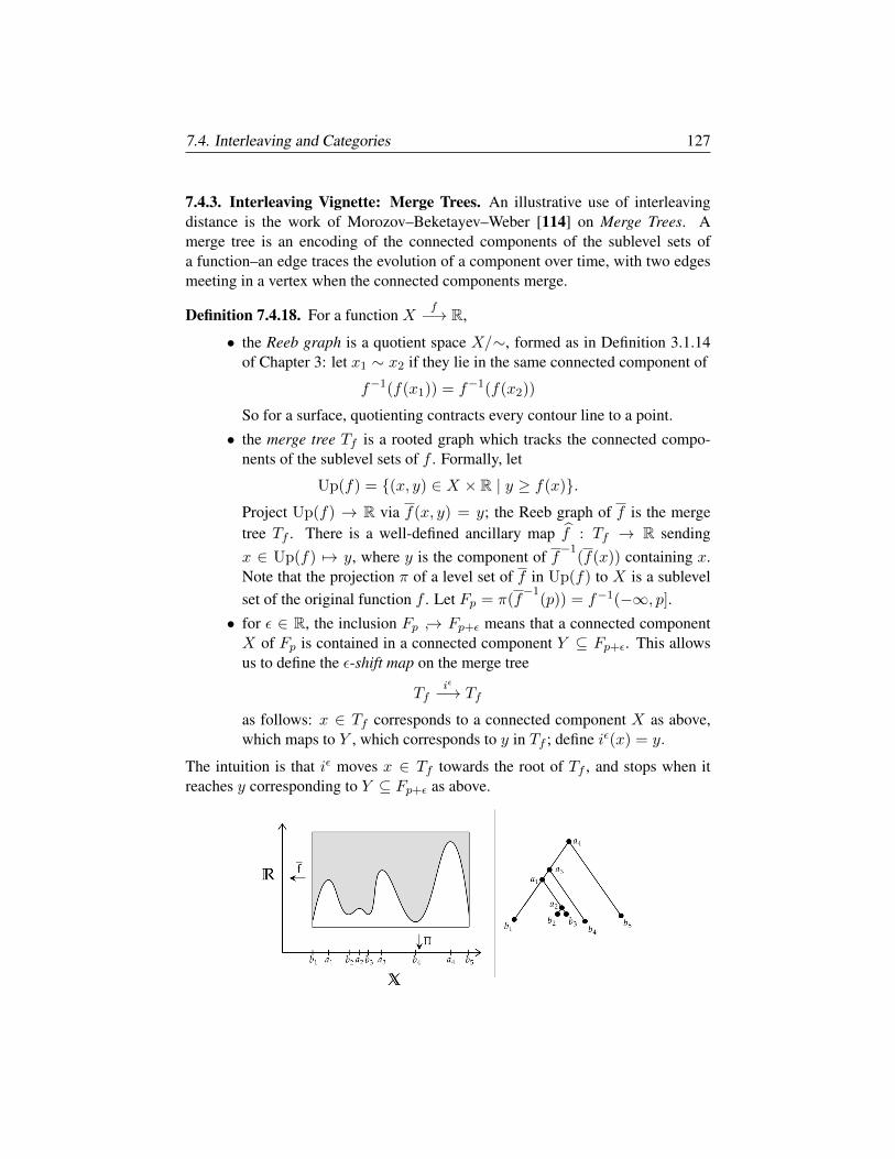
7.4. Interleaving and Categories 127
7.4.3. Interleaving Vignette: Merge Trees. An illustrative use of interleavingdistance is the work of Morozov–Beketayev–Weber [114] on Merge Trees. Amerge tree is an encoding of the connected components of the sublevel sets ofa function–an edge traces the evolution of a component over time, with two edgesmeeting in a vertex when the connected components merge.
Definition 7.4.18. For a function Xf−→ R,
• the Reeb graph is a quotient space X/∼, formed as in Definition 3.1.14of Chapter 3: let x1 ∼ x2 if they lie in the same connected component of
f−1(f(x1)) = f−1(f(x2))
So for a surface, quotienting contracts every contour line to a point.
• the merge tree Tf is a rooted graph which tracks the connected compo-nents of the sublevel sets of f . Formally, let
Up(f) = (x, y) ∈ X × R | y ≥ f(x).Project Up(f) → R via f(x, y) = y; the Reeb graph of f is the mergetree Tf . There is a well-defined ancillary map f : Tf → R sendingx ∈ Up(f) 7→ y, where y is the component of f
−1(f(x)) containing x.
Note that the projection π of a level set of f in Up(f) to X is a sublevelset of the original function f . Let Fp = π(f
−1(p)) = f−1(−∞, p].
• for ε ∈ R, the inclusion Fp → Fp+ε means that a connected componentX of Fp is contained in a connected component Y ⊆ Fp+ε. This allowsus to define the ε-shift map on the merge tree
Tfiε−→ Tf
as follows: x ∈ Tf corresponds to a connected component X as above,which maps to Y , which corresponds to y in Tf ; define iε(x) = y.
The intuition is that iε moves x ∈ Tf towards the root of Tf , and stops when itreaches y corresponding to Y ⊆ Fp+ε as above.
128 7. Persistent Homology
In order to relate a pair of merge trees Tf and Tg, we consider interleaving mapsbetween the two. Continuous maps
Tfαε−→ Tg and Tg
βε−→ Tf
are ε-compatible if they satisfy the criteria of Definition 7.4.7, where
g(αε(x)) = f(x) + ε f(βε(y)) = g(y) + εβε αε = i2ε αε βε = j2ε,
with Tfi2ε−→ Tf and Tg
j2ε−→ Tg are the 2ε-shift maps in their trees. The interleav-ing distance on merge trees comes from Definition 7.4.7:
dI(Tf , Tg) = infε | there exist ε− compatible maps as above.
Here are the two main results of [114] on interleaving distance for merge trees:
Theorem 7.4.19. For f, g : X −→ R, the merge trees Tf and Tg satisfy
dI(Tf , Tg) ≤ ||f − g||∞.
Proof. We interleave the sublevel sets of f and g. If ‖f − g‖∞ = ε then sinceFp = f−1(−∞, p] and Gq = g−1(−∞, q],
Fp ⊆ Gp+ε ⊆ Fp+2ε.
Now,p ∈ Tf corresponds to a component Xp ⊆ Fp ⊆ Gp+ε,
so the component Xp is contained in some component Yp+ε of Gp+ε. If q is thepoint of Tg corresponding to Yp+ε, then
αε(p) = q.
By construction, if f(p) = p then g(αε(p)) = p + ε. The shift maps are inducedby inclusions so
βε αε = i2ε and αε βε = j2ε
and we conclude that dI(Tf , Tg) ≤ ε.
There is a similar result for bottleneck distance. The proof uses a version of theresult of [39], simplified to the setting p = 0. Let f, g : X −→ R be tame functionssuch that there are ε-interleavings as below
H0(Ft)φε−→ H0(Gt+ε) and H0(Gt)
ψε−→ H0(Ft+ε),
which commute with the inclusion maps. Then
dB(D0(f), D0(g)) ≤ ε.
Theorem 7.4.20. For f, g : X −→ R, the merge trees Tf and Tg satisfy
dB(D0(f), D0(g)) ≤ dI(Tf , Tg)
7.4. Interleaving and Categories 129
Proof. Because merge trees contract sublevel sets to points and H0 measures thenumber of connected components,
Xf−→ R and Tf
f−→ R
have the same zero-dimensional persistence diagrams
D0(f) = D0(f).
Hence it suffices to show that
dB(D0(f), D0(g)) ≤ dI(Tf , Tg) = ε.
Since dI(Tf , Tg) = ε, we have maps
Tfαε−→ Tg and Tg
βε−→ Tf
which commute with the induced inclusion maps. So in particular, f−1(−∞, a]and g−1(−∞, a] are ε-interleaved, hence so are the corresponding groups
H0(f−1(−∞, a]) and H0(g−1(−∞, a]).
Applying the variant of [39] described above concludes the proof.
7.4.4. Zigzag Persistence and Quivers. We close with another connection be-tween TDA and category theory. Our standard setup thus far has involved fatteningthe dots in a point cloud, yielding a filtered topological space, with
Xε → Xε′ when ε ≤ ε′.
What about the case where we have a parameterized family of topological spacesthat can both dilate and contract? Such situations arise naturally: suppose forexample the parameter ε represents time, and Xε is the aorta. To deal with suchsituations, we are led to
Xε ←→ Xε′ when ε ≤ ε′,
where←→ means either Xε ← Xε′ or Xε → Xε′ . Passing to the level of vectorspaces, we have a diagram
(7.4.5) V1 ←→ V2 ←→ V3 ←→ · · ·VnIn [26] Carlsson–de Silva introduce Zigzag Persistence to handle cases of this type:it turns out that the theory of quiver representations provides the perfect frameworkfor addressing the situation. We close by giving a brief sketch of the ingredientsthat go into developing the theory of zigzag persistence.
Definition 7.4.21. A quiver is a directed graph as in Definition 3.4.1 (note thatloops and multiple edges are allowed). A quiver representation is an assignmentof a vector space to each vertex, and a linear map to each directed edge.
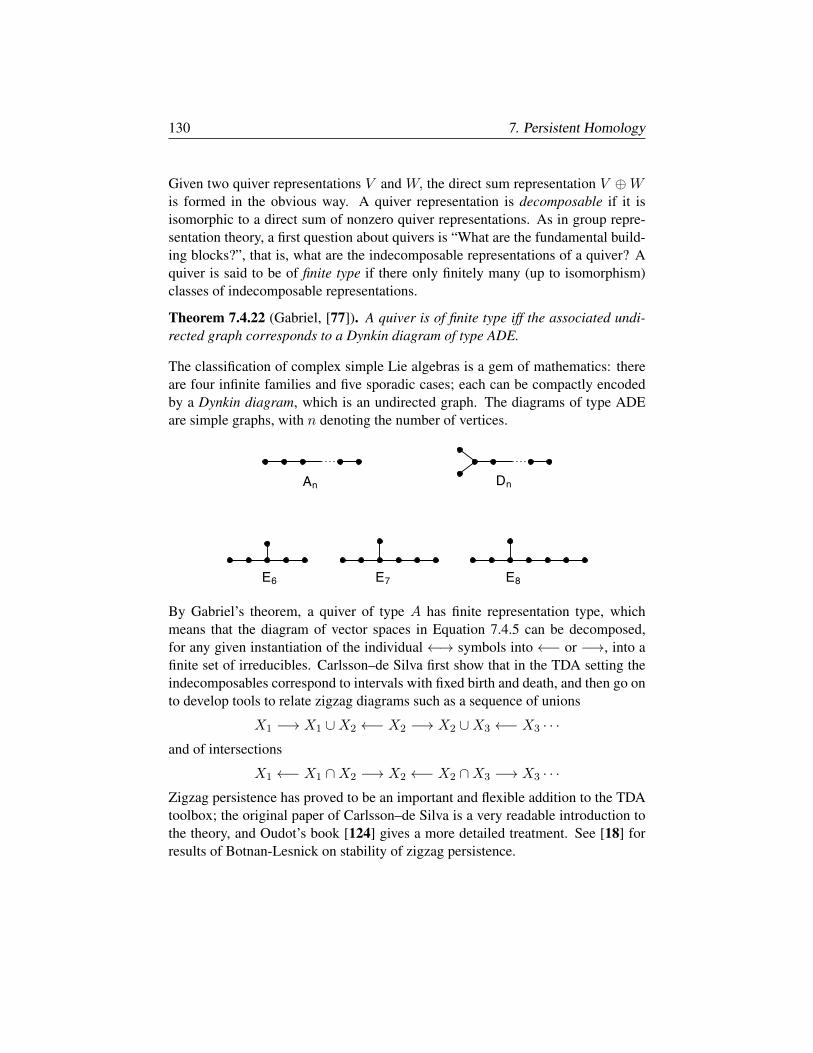
130 7. Persistent Homology
Given two quiver representations V and W, the direct sum representation V ⊕Wis formed in the obvious way. A quiver representation is decomposable if it isisomorphic to a direct sum of nonzero quiver representations. As in group repre-sentation theory, a first question about quivers is “What are the fundamental build-ing blocks?”, that is, what are the indecomposable representations of a quiver? Aquiver is said to be of finite type if there only finitely many (up to isomorphism)classes of indecomposable representations.
Theorem 7.4.22 (Gabriel, [77]). A quiver is of finite type iff the associated undi-rected graph corresponds to a Dynkin diagram of type ADE.
The classification of complex simple Lie algebras is a gem of mathematics: thereare four infinite families and five sporadic cases; each can be compactly encodedby a Dynkin diagram, which is an undirected graph. The diagrams of type ADEare simple graphs, with n denoting the number of vertices.
DnAn
E6 E7 E8
By Gabriel’s theorem, a quiver of type A has finite representation type, whichmeans that the diagram of vector spaces in Equation 7.4.5 can be decomposed,for any given instantiation of the individual←→ symbols into←− or −→, into afinite set of irreducibles. Carlsson–de Silva first show that in the TDA setting theindecomposables correspond to intervals with fixed birth and death, and then go onto develop tools to relate zigzag diagrams such as a sequence of unions
X1 −→ X1 ∪X2 ←− X2 −→ X2 ∪X3 ←− X3 · · ·and of intersections
X1 ←− X1 ∩X2 −→ X2 ←− X2 ∩X3 −→ X3 · · ·Zigzag persistence has proved to be an important and flexible addition to the TDAtoolbox; the original paper of Carlsson–de Silva is a very readable introduction tothe theory, and Oudot’s book [124] gives a more detailed treatment. See [18] forresults of Botnan-Lesnick on stability of zigzag persistence.
Chapter 8
Multiparameter PersistentHomology
In [33], Carlsson–Zomorodian introduced an extension of persistent homology tothe setting of filtrations depending on more than one parameter. Near the end oftheir paper, they write
“Our study of multigraded objects shows that no complete dis-crete invariant exists for multidimensional persistence. We stilldesire a discriminating invariant that captures persistent informa-tion, that is, homology classes with large persistence.”
In this chapter we use tools of multigraded algebra to explore multiparameter per-sistent homology (MPH). While there are natural analogs of the free summands(long bars) and torsion components (short bars) of persistent homology, a newphenomenon arises. In particular, there are intermediate components, which arenot full dimensional (not long bars), but do not die in high degree (not short bars).
In §3 of this chapter, we introduce the associated primes of a module, whichprovide a useful tool for analyzing multiparameter persistent homology. Just aspersistent homology is a Z-graded module over K[x], an MPH module with n-parameters is a Zn-graded moduleM over K[x1, . . . , xn]. This strongly constrainsthe associated primes of M , and implies that M has an interpretation in terms oftranslates of coordinate subspaces. This chapter covers
• Definition and Examples.
• Graded algebra, Hilbert function, series, polynomial.
• Associated Primes and Zn-graded modules.
• Filtrations and Ext.
The recent paper of Botnan-Lesnick [19] gives a state of the art survey of MPH.
131
132 8. Multiparameter Persistent Homology
8.1. Definition and Examples
In this section we define multiparameter persistent homology; while the definitionsare a bit lengthy the thing to keep in mind is that the constructions are simply theZn-graded analogs of persistent homology. We illustrate this by working throughan example from [33] in detail. The subsequent sections introduce the tools frommultigraded algebra used in [88] to analyze multiparameter persistent homology.
8.1.1. Multiparameter persistence. This section develops MPH, following [33].
Definition 8.1.1. Denote by Zn the set of n-tuples of natural numbers, and definethe following partial order on Zn: for any pair of elements u,v ∈ Zn we defineu 4 v iff ui ≤ vi for all i = 1, . . . n, where we write u = (u1, . . . , un) andv = (v1, . . . , vn). Given a collection of simplicial complexes ∆uu∈Zn indexedby Zn, we say that ∆uu∈Zn is an n-filtration if whenever uv we have that∆u ⊆ ∆v. If there exists u′ ∈ Zn such that ∆u = ∆u′ for all u < u′, then wesay that the n-filtration stabilizes. A multifiltration is an n-filtration for some n. Itis possible to grade over other posets, but we shall focus on Zn.
An n-filtered simplicial complex is a simplicial complex ∆ together with amultifiltration ∆uu∈Zn that stabilizes and such that ∆ = ∪u∈Zn∆u. An n-filtered simplicial complex (∆, ∆uu∈Zn) is finite if ∆ is finite. A multifilteredsimplicial complex is an n-filtered simplicial complex for some n ≥ 1.
Given a multifiltered simplicial complex (∆, ∆uu∈Zn), for each x ∈ ∆ wecall the minimal elements u ∈ Zn (with respect to the partial order ) at which itenters the filtration its entry degrees. If every x ∈ ∆ has exactly one entry degreewe call the multifiltered space one-critical.
Let ∆ be a multifiltered simplicial complex, and let i = 0, 1, 2, . . . . For anyu ∈ Zn denote by Ci(∆u) the K-vector space with basis given by the i-simplicesof ∆u, and similarly byHi(∆u) the ith simplicial homology with coefficients in K.Whenever uv we have that the inclusion maps ∆u → ∆v induce K-linear mapsψu,v : Ci(∆u) → Ci(∆v) and φu,v : Hi(∆u) → Hi(∆v) such that wheneveruwv we have that ψw,v ψu,w = ψu,v, and similarly φw,v φu,w = φu,v.We thus give the following definition:
Definition 8.1.2. Let ∆ be a multifiltered simplicial complex. The ith-chain mod-ule of ∆ over K is the tuple
(Ci(∆u)u∈Zn , ψu,v : Ci(∆u)→ Ci(∆v)uv) .
Similarly, the simplicial homology with coefficients in K of ∆ is the tuple
(Hi(∆u)u∈Zn , φu,v : Hi(∆u)→ Hi(∆v)uv),
where the maps ψu,v and φu,v are those induced by the inclusions.
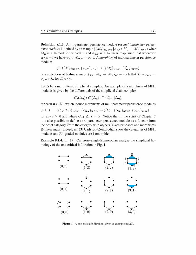
8.1. Definition and Examples 133
Definition 8.1.3. An n-parameter persistence module (or multiparameter persis-tence module) is defined by an n-tuple (Muu∈Zn , φu,v : Mu →Mvuv) whereMu is a K-module for each u and φu,v is a K-linear map, such that wheneveruwv we have φw,v φu,w = φu,v. A morphism of multiparameter persistencemodules
f : (Muu∈Zn , φu,vuv)→(M ′uu∈Zn , φ′u,vuv
)is a collection of K-linear maps fu : Mu → M ′uu∈Zn such that fv φu,v =φ′u,v fu for all uv.
Let ∆ be a multifiltered simplicial complex. An example of a morphism of MPHmodules is given by the differentials of the simplicial chain complex
C•(∆u) : Ci(∆u)di−→ Ci−1(∆u),
for each u ∈ Zn, which induce morphisms of multiparameter persistence modules
(8.1.1) (Ci(∆u)u∈Zn , ψu,vuv)→ (Ci−1(∆u)u∈Zn , ψu,vuv)
for any i ≥ 0 and where C−1(∆u) = 0. Notice that in the spirit of Chapter 7it is also possible to define an n-parameter persistence module as a functor fromthe poset category Zn to the category with objects K-vector spaces and morphismsK-linear maps. Indeed, in [33] Carlsson–Zomorodian show the categories of MPHmodules and Zn-graded modules are isomorphic.
Example 8.1.4. In [29], Carlsson–Singh–Zomorodian analyze the simplicial ho-mology of the one-critical bifiltration in Fig. 1.
(0, 0)
e
f
cb
••
••
(1, 0)
d••
••
•(2, 0)
••
••
•(3, 0)
••
••
•
(0, 1)
••
••
(1, 1)
a
••
••
•
•
(2, 1)
••
••
•
•
(3, 1)
••
••
•
•
(0, 2)
••
••
(1, 2)
••
••
•
•
(2, 2)
••
••
•
•
(3, 2)
••
••
•
•
e
f
cb
a
d
Figure 1. A one-critical bifiltration, given as example in [29].
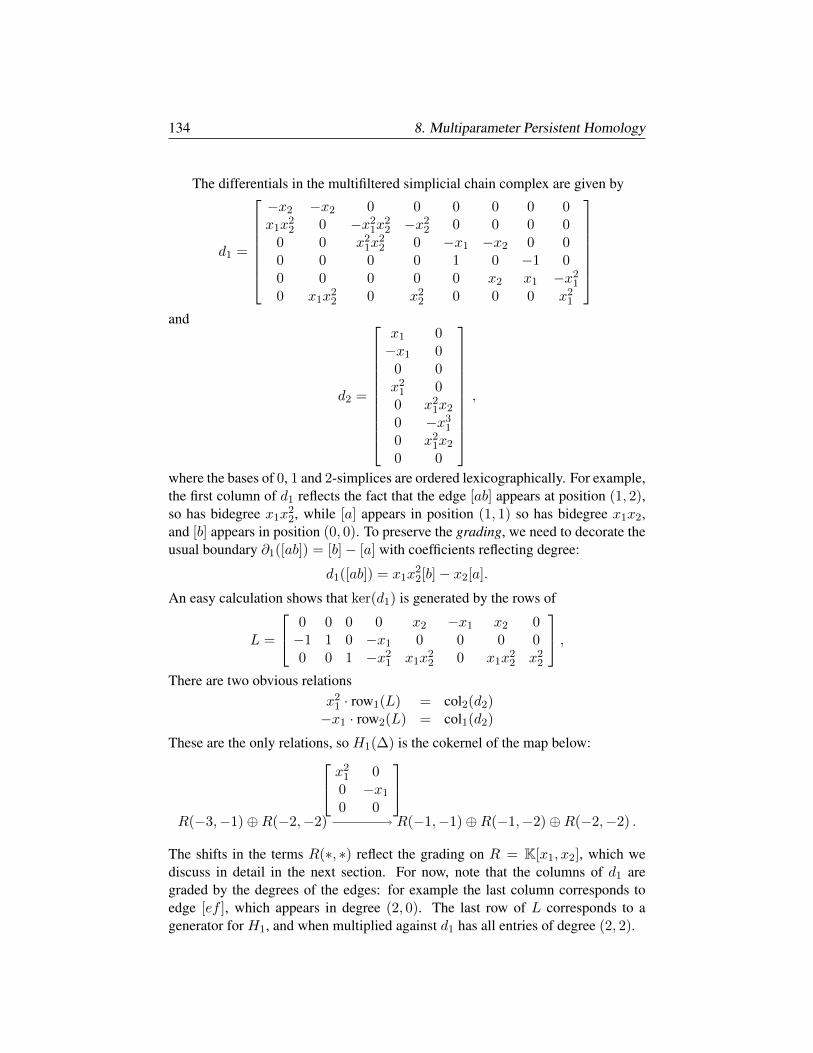
134 8. Multiparameter Persistent Homology
The differentials in the multifiltered simplicial chain complex are given by
d1 =
−x2 −x2 0 0 0 0 0 0x1x
22 0 −x2
1x22 −x2
2 0 0 0 00 0 x2
1x22 0 −x1 −x2 0 0
0 0 0 0 1 0 −1 00 0 0 0 0 x2 x1 −x2
1
0 x1x22 0 x2
2 0 0 0 x21
and
d2 =
x1 0−x1 0
0 0x2
1 00 x2
1x2
0 −x31
0 x21x2
0 0
,
where the bases of 0, 1 and 2-simplices are ordered lexicographically. For example,the first column of d1 reflects the fact that the edge [ab] appears at position (1, 2),so has bidegree x1x
22, while [a] appears in position (1, 1) so has bidegree x1x2,
and [b] appears in position (0, 0). To preserve the grading, we need to decorate theusual boundary ∂1([ab]) = [b]− [a] with coefficients reflecting degree:
d1([ab]) = x1x22[b]− x2[a].
An easy calculation shows that ker(d1) is generated by the rows of
L =
0 0 0 0 x2 −x1 x2 0−1 1 0 −x1 0 0 0 00 0 1 −x2
1 x1x22 0 x1x
22 x2
2
,There are two obvious relations
x21 · row1(L) = col2(d2)−x1 · row2(L) = col1(d2)
These are the only relations, so H1(∆) is the cokernel of the map below:
R(−3,−1)⊕R(−2,−2) R(−1,−1)⊕R(−1,−2)⊕R(−2,−2) .
x21 0
0 −x1
0 0
The shifts in the terms R(∗, ∗) reflect the grading on R = K[x1, x2], which wediscuss in detail in the next section. For now, note that the columns of d1 aregraded by the degrees of the edges: for example the last column corresponds toedge [ef ], which appears in degree (2, 0). The last row of L corresponds to agenerator for H1, and when multiplied against d1 has all entries of degree (2, 2).
8.2. Graded algebra, Hilbert function, series, polynomial 135
8.2. Graded algebra, Hilbert function, series, polynomial
In certain situations, graded algebra turns complicated questions about algebraicobjects into questions about vector spaces. This section covers the main invariantsof graded modules: the Hilbert function and the Hilbert series, as well as how toread off a first measure of the size of a module–the rank. For a module M over aPID, the rank of M is the rank of the free summand, so corresponds in TDA to thenumber of long bars. In particular, the rank of an MPH module is a natural choiceof proxy for the number of long bars.
Definition 8.2.1. Let R be an integral domain, K = R〈0〉 the field of fractions asin Exercise 2.3.2, and M a finitely generated R-module. The rank of M is
rank(M) = dimK(M ⊗R K) = dimK(M〈0〉)
Example 8.2.2. The Z-module Zmn⊕i=1
Z/qi has rank m.
Definition 8.2.3. Let G be an abelian group. A ring R is G-graded if
R =⊕g∈G
Rg,
where if ri ∈ Ri and rj ∈ Rj then
ri · rj ∈ Ri+j .
Note that each Ri is itself a module over R0. A graded module M over R is amodule with a direct sum decomposition
M =⊕g∈G
Mg,
where if ri ∈ Ri and mj ∈Mj then
ri ·mj ∈Mi+j .
For applications in topological data analysis, the case of interest is G = Zn. Forthese modules, we can determine the rank of a module from the growth rate of theHilbert Function.
Example 8.2.4. A polynomial ring R = K[x1, . . . , xn] is Z-graded. The compo-nent Ri is the R0 = K-vector space of polynomials f(x1, . . . , xn) such that everymonomial appearing f is of the same degree i, as in Exercise 2.4.16. A simpleinduction on the number of variables shows that
dimKRi =
(n− 1 + i
i
).
136 8. Multiparameter Persistent Homology
8.2.1. The Hilbert function. For a G-graded module M over a G-graded ringR with R0 = K a field, the Hilbert function of M records the dimensions of thevector spaces Mg, g ∈ G. Henceforth, we restrict to the case G = Zn.
Definition 8.2.5. Let M be a Zn-graded module over R = K[x1, . . . , xn]. TheHilbert function of M is the function HF (M,u) = dimKMu.
Example 8.2.6. For the polynomial ring R = K[x1, . . . , xn], the two most com-mon gradings are the Z-grading of Example 8.2.4, and the fine or Zn-grading. Inthe fine grading with u = (u1, . . . , un), Ru is one dimensional with basis xu. For1 ≤ r ≤ n there are other Zr-gradings possible. For example, consider the ringT = K[x1, . . . , x4], where x1, x2 have degree (1, 0) and x3, x4 have degree(0, 1). This is a Z2-grading (or bigrading). The bidegree (1, 2) component of T is
T(1,2) = Spanx1x23, x1x3x4, x1x
24, x2x
23, x2x3x4, x2x
24
A Zn-graded Hilbert function is an n-dimensional array, with the u = (u1, . . . , un)entry equal to the dimension of Mu. In the fine grading, the Hilbert function of Ritself is an n-dimensional array with a one in every position which has all indicesnon-negative, and zeroes elsewhere. The Hilbert function of R(−u) is the samearray, but with the origin translated to position u; this process is known as shifting.
Definition 8.2.7. For a finitely generatedR-moduleM , a free resolution is an exactsequence of free modules terminating in M :
· · · d3−→ F2d2−→ F1
d1−→ F0d0−→M−→0.
When working in the category of graded rings and graded modules, maps mustpreserve the graded structure: φ : M → N takes Mu → Nu.
Example 8.2.8. In Example 2.4.17 we considered the ideal I of 2× 2 minors of a2×3 matrixA =
[x y zy z w
]. If we gradeR by Z, then a free Z-graded resolution
for M = R/I is given by
0 −→ R(−3)2
x y−y −zz w
−−−−−−−−−−→ R(−2)3
[xz − y2 xw − yz yw − z2
]−−−−−−−−−−−−−−−−−−−−−−−−−→ R −→ R/I
Elements of the kernel of di are called ithsyzygies. In the special situation above,the first syzygies arise by stacking [x, y, z] or [y, z, w] as a third row of A; thedeterminant of the resulting 3 × 3 matrix has a repeat row, and hence yields asyzygy. The leftmost matrix has no kernel so the process stops. Since the map
F1 = R3 d1−→ R1 = F0
is multiplication by quadrics, to preserve the Z-grading, we must shift so that thedegrees of the generators of F1 have degree 2. Similarly, as the leftmost map d1 hasdegree one entries and maps onto a target generated in degree two, the generatorsof F2 are in degree three.
8.2. Graded algebra, Hilbert function, series, polynomial 137
In nice situations, free resolutions are actually finite; for a proof see [70].
Theorem 8.2.9. [Hilbert Syzygy Theorem] A finitely generated R = K[x1, . . . , xn]module M has a free resolution of length at most n.
Lemma 8.2.10. For a finitely generated graded R = K[x1, . . . , xn]-module Mwith free resolution F• as in Definition 8.2.7,
(a) HF (M,u) =∑i≥0
(−1)iHF (Fi,u)
(b) rankR(M) =∑i≥0
(−1)irankR(Fi).
Proof. The key point is that because the maps in a graded free resolution preservethe grading, the free resolution is exact in each graded degree. Since for eachdegree u, the degree u components of F• are an exact sequence of vector spacesover K, so (a) follows from Example 4.2.4. For part (b), by Theorem 8.2.9M has afinite free resolution. Tensoring the (finite) exact sequence of Definition 8.2.7 withthe field of fractions ofR is equivalent to localizing. By Theorem 2.3.3 localizationis exact, so (b) follows from Example 4.2.4.
Lemma 8.2.11. For a finitely generated Zn-graded R = K[x1, . . . , xn]-moduleM ,
rankR(M) = HF (M,u) for u 0 .
Proof. A finitely generated, Zn-graded free module F is of the form
F =m⊕j=1
R(−uj), with uj ∈ Zn.
Since HF (R(−uj),v) = 1 if v ≥ uj and 0 otherwise, when v ≥ uj for allj ∈ 1, . . . , n
HF (F,v) = n = rankR(F ).
By Theorem 8.2.9 M has a finite free resolution; apply Lemma 8.2.10.
Example 8.2.12. [Hilbert Polynomial] In the special case of a Z-graded ring Ras in Example 8.2.8, the Hilbert function of a graded R-module M is given by apolynomial when i ∈ Z is sufficiently large:
HF (M, i) = P (M, i) ∈ Q[i], when i 0.
This can be proved by induction on the number of variables, using the four termexact sequence
0 −→ ker(·xn) −→M(−1)·xn−→M −→ coker(·xn) −→ 0,
using that ker(·xn) and coker(·xn) are K[x1, . . . , xn−1]-modules. The polynomialP (M, i) has the form
P (M, i) =amm!
im + . . .+ a0, with m ≤ n− 1.
138 8. Multiparameter Persistent Homology
In the context of projective geometry with M = R/I as in Example 8.2.8, thedimension of V(I) is the degree of P (R/I, i), and the degree of V(I) is the (nor-malized) lead coefficient am. The dimension of V(I) is the number of times itcan be cut with a general hyperplane until we’re left with a set of points; the num-ber of points (with multiplicity, if V(I) is singular) is the degree of V(I). ByExample 8.2.4
P (R(−j), i) =
(n− 1 + i− j
n− 1
)Exercise 8.2.13. Use the free resolution which appears in Example 8.2.8 to showthat P (R/I, i) = 3i + 1. Thus the degree of V(I) is three, and the dimension isone. The corresponding curve in P3 is known as the twisted cubic. 8.2.2. The Hilbert series. The Hilbert series provides a compact way of packag-ing the data of the Hilbert function into a formal power series.
Definition 8.2.14. For a finitely generated R = K[x1, . . . , xn]-module M whichis Zn-graded, the multigraded Hilbert series of M is the formal power series inZ[[t1, . . . , tn]] defined as follows:
HS(M, t) =∑u∈Zn
HF (M,u)tu .
Inducting on the number of variables yields
(8.2.1) HS(R(−u), t) =tu∏n
i=1(1− ti).
By Lemma 8.2.10 the Hilbert function is additive on exact sequences, so this isalso true for the Hilbert series. Hence applying Theorem 8.2.9 we have
(8.2.2) HS(M, t) =
n∑i=0
(−1)iHS(Fi, t) .
For a finitely generated, multigraded R-module M , it follows from the HilbertSyzygy Theorem and Equations (8.2.1)–(8.2.2) that the multigraded Hilbert seriesof M is a rational polynomial of the form
(8.2.3) HS(M, t) =P (t1, . . . , tn)∏ni=1(1− ti)
.
The polynomial P (t1, . . . , tn) in Equation (8.2.3) is an invariant of the module.
Lemma 8.2.15. For a finitely generated graded R = K[x1, . . . , xn]-module M ,rankR(M) is equal to P (1), where P is as in Equation 8.2.3.
Proof. To see that rankR(M) is the numerator of HS(M, t) evaluated at 1, notethat it holds for free modules by Equation (8.2.1). Now apply Lemma 8.2.10.

8.2. Graded algebra, Hilbert function, series, polynomial 139
Example 8.2.16. Note that if M is a one-parameter persistence module, we have
(8.2.4) HS(M, t) =
∑long bars t
bl
(1− t)+
∑short bars(tbs − tds)
(1− t)
where bl is the birth time for a long bar, bs the birth time for a short bar, and ds thedeath time of a short bar. So
HS(M, 1) = rankR(M)
is indeed the number of long bars.
We close by revisiting Example 8.1.4
Example 8.2.17. In Example 8.1.4, H1(∆) = coker(δ1), with
δ1 =
x21 0
0 −x1
0 0
It is easy to see that δ1 has no kernel itself, so we have a free resolution for H1(∆)
0 −→ F1δ1−→ F0 −→ H1(∆) −→ 0,
soHS(H1(∆), t) = HS(F0, t)−HS(F1, t)
=t1t2+t1t22+t21t
22
(1−t1)(1−t2) −t31t2+t21t
22
(1−t1)(1−t2)
=t1t2+t1t22−t31t2(1−t1)(1−t2) .
It follows that P (H1(∆),1) = 1, so rank(H1(∆)) = 1. In fact, because in thiscase the presentation is so simple, we see that
H1(∆) ' (R(−1,−1)/〈x21〉)⊕
(R(−1,−2)/〈x1〉)⊕
R(−2,−2).
In particular, note that the first two terms
(R(−1,−1)/〈x21〉)⊕
(R(−1,−2)/〈x1〉)
are not free, but also do not vanish in high degree in the x2 variable. For anyprincipal ideal 〈f〉 with deg(f) = u, we have an exact sequence:
0 −→ R(−u)·f−→ R −→ R/〈f〉 −→ 0,
soHS(R/〈f〉, t) =
1− tu∏ni=1(1− ti)
.
The next section introduces associated primes, which will provide a way to un-derstand the structure of MPH modules, which generally do not decompose as adirect sum as they do in this example. As a module, the summandR(−1,−2)/〈x1〉above is supported in the sense of Definition 8.3.4 on V(x1).
Exercise 8.2.18. Show HS(R(−1,−2)/〈x1〉, t) =t1t221−t2 .
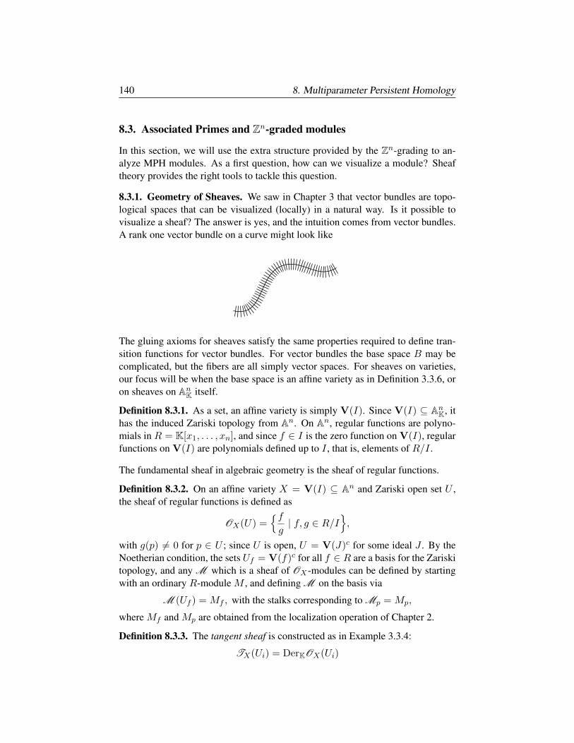
140 8. Multiparameter Persistent Homology
8.3. Associated Primes and Zn-graded modules
In this section, we will use the extra structure provided by the Zn-grading to an-alyze MPH modules. As a first question, how can we visualize a module? Sheaftheory provides the right tools to tackle this question.
8.3.1. Geometry of Sheaves. We saw in Chapter 3 that vector bundles are topo-logical spaces that can be visualized (locally) in a natural way. Is it possible tovisualize a sheaf? The answer is yes, and the intuition comes from vector bundles.A rank one vector bundle on a curve might look like
The gluing axioms for sheaves satisfy the same properties required to define tran-sition functions for vector bundles. For vector bundles the base space B may becomplicated, but the fibers are all simply vector spaces. For sheaves on varieties,our focus will be when the base space is an affine variety as in Definition 3.3.6, oron sheaves on AnK itself.
Definition 8.3.1. As a set, an affine variety is simply V(I). Since V(I) ⊆ AnK, ithas the induced Zariski topology from An. On An, regular functions are polyno-mials in R = K[x1, . . . , xn], and since f ∈ I is the zero function on V(I), regularfunctions on V(I) are polynomials defined up to I , that is, elements of R/I .
The fundamental sheaf in algebraic geometry is the sheaf of regular functions.
Definition 8.3.2. On an affine variety X = V(I) ⊆ An and Zariski open set U ,the sheaf of regular functions is defined as
OX(U) =fg| f, g ∈ R/I
,
with g(p) 6= 0 for p ∈ U ; since U is open, U = V(J)c for some ideal J . By theNoetherian condition, the sets Uf = V(f)c for all f ∈ R are a basis for the Zariskitopology, and any M which is a sheaf of OX -modules can be defined by startingwith an ordinary R-module M , and defining M on the basis via
M (Uf ) = Mf , with the stalks corresponding to Mp = Mp,
where Mf and Mp are obtained from the localization operation of Chapter 2.
Definition 8.3.3. The tangent sheaf is constructed as in Example 3.3.4:
TX(Ui) = DerKOX(Ui)

8.3. Associated Primes and Zn-graded modules 141
A point p ∈ X is smooth if the stalk TX,p is a free OX,p-module; X is smooth ifevery point is a smooth point. This mirrors the construction of the tangent bundleof an n-dimensional real manifold M . In this situation, K = R and there is a coverof M by open sets Ui diffeomorphic to Rn. The transition maps φij appearing inDefinition 3.2.2 are C∞ maps between charts, and the fibers are Rn.
Definition 8.3.4. The support of an R-module M consists of the prime ideals Psuch that MP 6= 0.
When M is a finitely generated R-module, a prime ideal P is in the support of Miff ann(M) ⊆ P . If M is generated by m1, . . . ,mk, then there is a surjection
Rk −→M −→ 0.
Localizing at a prime P makes elements of R outside P invertible, therefore ifann(M) 6⊆ P , then some element r ∈ ann(M) is a unit in RP . But a unit canannihilate every element of MP only if MP = 0.
8.3.2. Associated Primes and Primary Decomposition. We defined the varietyof an ideal I ⊆ K[x1, . . . , xn] in Chapter 2:
V(I) = p ∈ Kn | f(p) = 0 for all f ∈ I
Example 8.3.5. For I = 〈x2 − x, xy − x〉 ⊂ R[x, y], V(I) ⊆ R2 is picturedbelow:
So V(I) consists of the line V(x) and the point V(x− 1, y − 1). Notice that
I = 〈x〉 ∩ 〈x− 1, y − 1〉
By Theorem 2.2.11, I is prime iff R/I is a domain, and since
R[x, y]/〈x〉 ' R[y] and R[x, y]/〈x− 1, y − 1〉 ' R
are both domains, we see that I is the intersection of two prime ideals.
It is clearly too much to hope that any ideal is an intersection of prime ideals:
〈x2〉 ⊆ R[x]
cannot be written as an intersection of prime ideals. But it turns out that any ideal ina Noetherian ring has a decomposition as a finite intersection of irreducible ideals,which appeared in Definition 2.2.9. Recall an ideal I is irreducible if it is not theintersection of two proper ideals, each strictly containing I .
142 8. Multiparameter Persistent Homology
Theorem 8.3.6. In a Noetherian ring R, any ideal I can be written as
I =
n⋂i=1
Ii,
with Ii irreducible.
Proof. Let Σ be the set of all ideals which cannot be written as a finite intersectionof irreducible ideals. Since R is Noetherian, Σ has a maximal element I ′. Since I ′
is reducible,I ′ = J1 ∩ J2
with I ′ ( J1 and I ′ ( J2. Since I ′ is maximal, neither J1 nor J2 are in Σ. Henceboth J1 and J2 can be written as finite intersections of irreducibles, thus I ′ is afinite intersection of irreducibles, a contradiction.
Primary ideals also appeared in Definition 2.2.9; Q is primary if
xy ∈ Q⇒ x ∈ Q or yn ∈ Q for some n.
In a Noetherian ring an irreducible ideal is primary ([133] Lemma 1.3.3), so wehave
Theorem 8.3.7. In a Noetherian ring R, any ideal I can be written as
I =n⋂i=1
Qi,
with Qi primary.
It follows immediately from the definition that the radical of a primary ideal isprime, since x or yn ∈ Q⇒ x or y ∈
√Q.
Definition 8.3.8. For a primary decomposition
I =n⋂i=1
Qi
the Pi =√Qi appearing in this decomposition are the Associated Primes of I .
Exercise 8.3.9. Show primary decomposition is not unique:
〈xy, x2〉 = 〈x2, y〉 ∩ 〈x〉= 〈x2, xy, y2〉 ∩ 〈x〉
In particular, show 〈x2, y〉 and 〈x2, xy, y2〉 are primary. What are the associatedprimes? There is a version of associated primes for an R-module M :
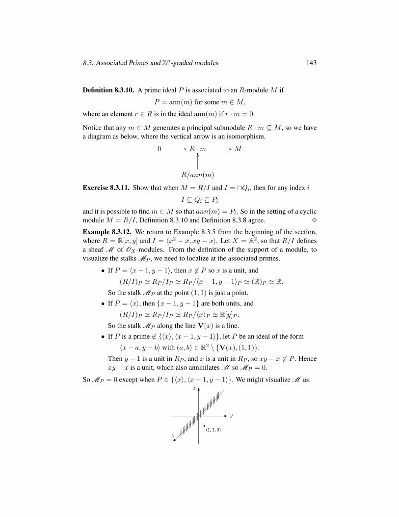
8.3. Associated Primes and Zn-graded modules 143
Definition 8.3.10. A prime ideal P is associated to an R-module M if
P = ann(m) for some m ∈M,
where an element r ∈ R is in the ideal ann(m) if r ·m = 0.
Notice that any m ∈ M generates a principal submodule R ·m ⊆ M , so we havea diagram as below, where the vertical arrow is an isomorphism.
0 // R ·m // M
R/ann(m)
OO
Exercise 8.3.11. Show that when M = R/I and I = ∩Qi, then for any index i
I ⊆ Qi ⊆ Piand it is possible to find m ∈M so that ann(m) = Pi. So in the setting of a cyclicmodule M = R/I , Definition 8.3.10 and Definition 8.3.8 agree. Example 8.3.12. We return to Example 8.3.5 from the beginning of the section,where R = R[x, y] and I = 〈x2 − x, xy − x〉. Let X = A2, so that R/I definesa sheaf M of OX -modules. From the definition of the support of a module, tovisualize the stalks MP , we need to localize at the associated primes.
• If P = 〈x− 1, y − 1〉, then x 6∈ P so x is a unit, and
(R/I)P ' RP /IP ' RP /〈x− 1, y − 1〉P ' (R)P ' R.So the stalk MP at the point (1, 1) is just a point.
• If P = 〈x〉, then x− 1, y − 1 are both units, and
(R/I)P ' RP /IP ' RP /〈x〉P ' R[y]P .
So the stalk MP along the line V(x) is a line.
• If P is a prime 6∈ 〈x〉, 〈x− 1, y − 1〉, let P be an ideal of the form
〈x− a, y − b〉 with (a, b) ∈ R2 \ V(x), (1, 1).Then y − 1 is a unit in RP , and x is a unit in RP , so xy − x 6∈ P . Hencexy − x is a unit, which also annihilates M so MP = 0.
So MP = 0 except when P ∈ 〈x〉, 〈x− 1, y − 1〉. We might visualize M as:
144 8. Multiparameter Persistent Homology
Definition 8.3.13. For a Noetherian ring R, the dimension (or Krull dimension) is
dim(R) = supnP0 ( P1 ( · · ·Pn ( R with the Pi prime ideals in R.
If R is an integral domain (which will always be the case for us), there is a uniquecommon starting point for chains as above: 0 = P0. Note that if R is not Noether-ian, then there can be infinite ascending proper chains of ideals.
Definition 8.3.14. Let R be a ring and I an ideal in R. The codimension of I is
supmP0 ( P1 ( P2 ( · · ·Pm ⊆ I
Example 8.3.15. For R = K[x1, . . . , xn], since
0 ⊆ 〈x1〉 ⊆ 〈x1, x2〉 ⊆ · · · ⊆ 〈x1, . . . , xn〉
is a proper chain of prime ideals, dim(R) ≥ n; it is not hard to show this is anequality. Consider the ideal
I = 〈x1, . . . , xm〉 ⊆ R.
From the definition, I has codimension at least m, and this too is an equality.Geometric mnemonic: V(I) ⊆ Kn is a linear space defined by the vanishing ofm independent linear forms, so is of dimension n − m, hence of complimentarydimension m. So we have
codim(I) = dim(V(I)) ⊆ Kn.
A word of caution: If I is defined by homogeneous polynomials and we workprojectively in Pn−1, then the dimension of V(I) as a projective variety is one lessthan the dimension as a variety in Kn. For example V(x0, x1) defines a plane inA4 or a line in P3, and 〈x0, x1〉 is of codimension two.
8.3.3. Additional structure in the Zn-graded setting. For Z-graded rings andmodules as in Example 8.2.8, we noted that maps also have to preserve gradings;this also applies to Zn-graded modules.
Theorem 8.3.16. The only Zn-graded prime ideals in R = K[x1, . . . , xn] are
(8.3.1) P = 〈xi0 , . . . , xir〉.
Proof. In the Zn-grading, the only polynomial of degree u = (u1, . . . , un) is
xu = xu11 · · ·x
unn
Hence, the only Zn-homogeneous ideals are ideals generated by monomials. Aprime ideal P cannot contain a monomial of degree two or more as a minimalgenerator, since if x1x2 ∈ P then x1 ∈ P or x2 ∈ P . Hence a prime ideal P isgenerated by monomials iff P is generated by a subset of the variables.
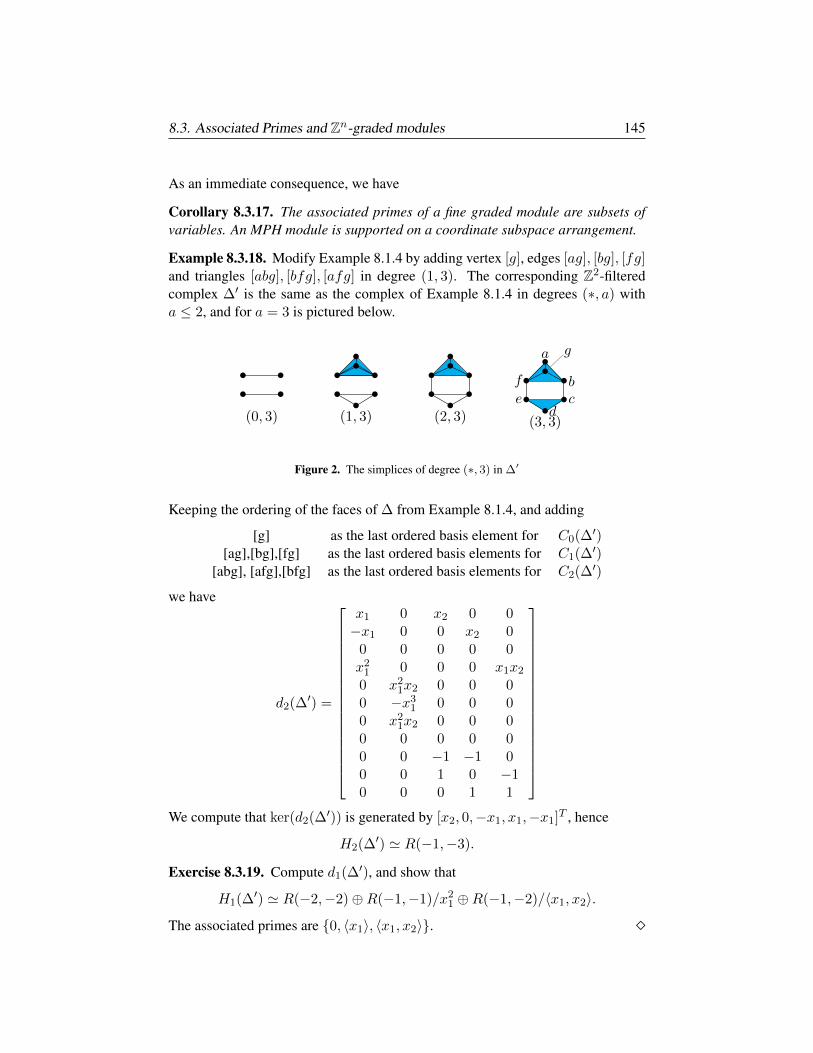
8.3. Associated Primes and Zn-graded modules 145
As an immediate consequence, we have
Corollary 8.3.17. The associated primes of a fine graded module are subsets ofvariables. An MPH module is supported on a coordinate subspace arrangement.
Example 8.3.18. Modify Example 8.1.4 by adding vertex [g], edges [ag], [bg], [fg]and triangles [abg], [bfg], [afg] in degree (1, 3). The corresponding Z2-filteredcomplex ∆′ is the same as the complex of Example 8.1.4 in degrees (∗, a) witha ≤ 2, and for a = 3 is pictured below.
(0, 3)
••
••
(1, 3)
••
••
••
•(2, 3)
••
••
••
•(3, 3)
g
••
••
•
••
e
f
cb
a
d
Figure 2. The simplices of degree (∗, 3) in ∆′
Keeping the ordering of the faces of ∆ from Example 8.1.4, and adding
[g] as the last ordered basis element for C0(∆′)[ag],[bg],[fg] as the last ordered basis elements for C1(∆′)
[abg], [afg],[bfg] as the last ordered basis elements for C2(∆′)
we have
d2(∆′) =
x1 0 x2 0 0−x1 0 0 x2 0
0 0 0 0 0x2
1 0 0 0 x1x2
0 x21x2 0 0 0
0 −x31 0 0 0
0 x21x2 0 0 0
0 0 0 0 00 0 −1 −1 00 0 1 0 −10 0 0 1 1
We compute that ker(d2(∆′)) is generated by [x2, 0,−x1, x1,−x1]T , hence
H2(∆′) ' R(−1,−3).
Exercise 8.3.19. Compute d1(∆′), and show that
H1(∆′) ' R(−2,−2)⊕R(−1,−1)/x21 ⊕R(−1,−2)/〈x1, x2〉.
The associated primes are 0, 〈x1〉, 〈x1, x2〉.
146 8. Multiparameter Persistent Homology
8.4. Filtrations and Ext
The examples of MPH modules we’ve encountered so far have all decomposed asdirect sums, but this is atypical. In general, our goal will be to stratify or filter theMPH module, to obtain an analog of the barcode. We will use the associated primesto do this, which leads to the first question: in general, how do we identify elementsof Ass(M)? There are general algorithms for identifying the associated primes ofa Z-graded R = K[x1, . . . , xn]-module. However, these algorithms rely on theuse of Grobner bases [47], and in the worst case Grobner bases can require doublyexponential runtime. In the setting of multiparameter persistence, Corollary 8.3.17shows that an associated prime P of M is a subset of the variables. This placesextremely strong constraints on the structure of fine graded modules; in particular,there is a finite subset of possible associated primes.
The algorithm mentioned above for identifying associated primes uses the de-rived functor Ext, so this is the right time to skip to Chapter 9 and read §1 and§2 if you’re encountering Ext for the first time. Combining the abstract algebraanalysis using Ext with the strong constraints on the associated primes of a finegraded module will provide insight into the structure of MPH, as well as yieldingone candidate for a higher dimensional proxy for the barcode.
Theorem 8.4.1. For a finitely generated Z-graded R = K[x1 . . . , xn]-module M ,a prime ideal P of codimension c is in Ass(M) iff it is in Ass(Extc(M,R)).
Proof. See [71] for complete details, or [133] for a quick sketch.
Example 8.4.2. Let R = K[x1, x2] and M = R/I with I = 〈x21, x1x2〉. In
Exercise 8.3.9, we saw that the associated primes of I are 〈x1〉, 〈x1, x2〉, whichfollowed from the primary decomposition
I = 〈x21, x2〉 ∩ 〈x1〉.
Chapter 9 gives a recipe to compute Exti(M,R): take a free resolution F• forM , dropM from the sequence, applyHomR(•, R) to F•, and compute homology.This seems like an arduous task, until we roll up our sleeves and do it.
• Step 1: A free resolution for R/I is easy to do by hand:
0 −→ R
x2−x1
−−−−−−→ R2
[x21 x1x2
]−−−−−−−−−−→ R −→ R/I
• Step 2: dropping R/I and applying HomR(•, R)–which simply trans-poses the differentials–yields
0 −→ R
x21x1x2
−−−−−−−→ R2
[x2 −x1
]−−−−−−−−−→ R −→ 0
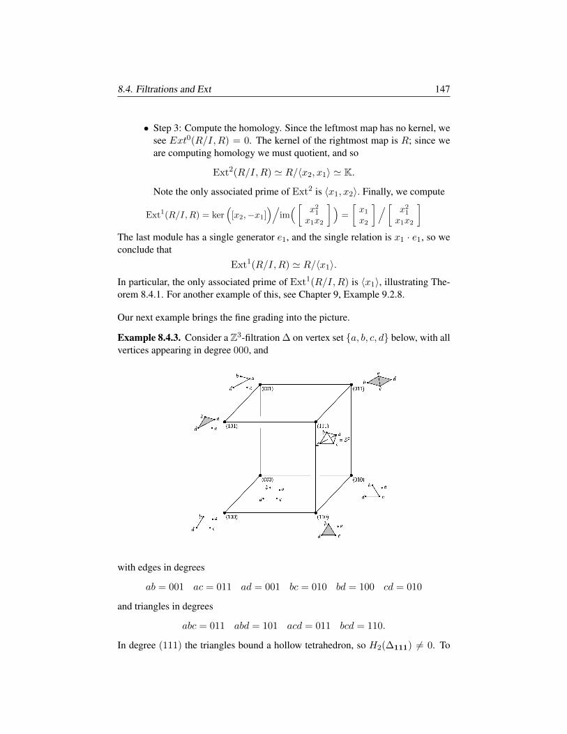
8.4. Filtrations and Ext 147
• Step 3: Compute the homology. Since the leftmost map has no kernel, wesee Ext0(R/I,R) = 0. The kernel of the rightmost map is R; since weare computing homology we must quotient, and so
Ext2(R/I,R) ' R/〈x2, x1〉 ' K.
Note the only associated prime of Ext2 is 〈x1, x2〉. Finally, we compute
Ext1(R/I,R) = ker(
[x2,−x1])/
im([
x21x1x2
])=
[x1x2
]/[x21x1x2
]The last module has a single generator e1, and the single relation is x1 · e1, so weconclude that
Ext1(R/I,R) ' R/〈x1〉.
In particular, the only associated prime of Ext1(R/I,R) is 〈x1〉, illustrating The-orem 8.4.1. For another example of this, see Chapter 9, Example 9.2.8.
Our next example brings the fine grading into the picture.
Example 8.4.3. Consider a Z3-filtration ∆ on vertex set a, b, c, d below, with allvertices appearing in degree 000, and
with edges in degrees
ab = 001 ac = 011 ad = 001 bc = 010 bd = 100 cd = 010
and triangles in degrees
abc = 011 abd = 101 acd = 011 bcd = 110.
In degree (111) the triangles bound a hollow tetrahedron, so H2(∆111) 6= 0. To
148 8. Multiparameter Persistent Homology
see this algebraically, with respect to the ordered bases above we have
d2(∆) =
x2 x1 0 0−1 0 1 00 −x1 −x2 0x3 0 0 x1
0 x3 0 −x2
0 0 x3 x1
and
d1(∆) =
−x3 −x2x3 −x3 0 0 0x3 0 0 −x2 −x1 00 x2x3 0 x2 0 −x2
0 0 x3 0 x1 x2
Exercise 8.4.4. Show that H2(∆) ' R(1, 1, 1) and H1(∆) = 0. The second column of d1 is a combination of the first and fourth columns so canbe dropped. A minimal presentation matrix for H0(∆) is given by
φ =
0 0 0 −x3 −x3−x1 −x2 0 x3 0
0 x2 −x2 0 0x1 0 x2 0 x3
A minimal free resolution for H0(∆) is given (omitting gradings) by
0 −→ R1
x3−x2x1
−−−−−−→ R3
−x2 −x3 0x1 0 −x3x1 0 −x30 −x1 −x20 x1 x2
−−−−−−−−−−−−−−−−→ R5 φ−→ R4 −→ H0(∆) −→ 0.
Exercise 8.4.5. Use the free resolution above to prove
Ext3(H0(∆), R) ' KExt2(H0(∆), R) ' 0Ext1(H0(∆), R) ' R/〈x2〉 ⊕R/〈x3〉Hom(H0(∆), R) ' R1
To do this, we transpose the differentials in the free resolution for H0(∆) andcompute homology. For example, to see that Ext3(H0(∆), R) ' K, just note thatthis module is the cokernel of transpose of the last map above
Ext3(H0(∆), R) = R1/im([x3,−x2, x1])
which is clearly K.

8.4. Filtrations and Ext 149
It will be useful to display the R-modules Exti(Hj(∆), R) in an (i+ 1)× (j + 1)array as below
Ext3(H0(∆), R) Ext3(H1(∆), R) Ext3(H2(∆), R)Ext2(H0(∆), R) Ext2(H1(∆), R) Ext2(H2(∆), R)Ext1(H0(∆), R) Ext1(H1(∆), R) Ext1(H2(∆), R)Hom(H0(∆), R) Hom(H1(∆), R) Hom(H2(∆), R)
Since we have shown that H2(∆) is free rank one, for Example 8.4.3 this arraytakes the form
K 0 00 0 0
Ext1(H1(∆), R) 0 0R1 0 R1
In Chapter 9, we’ll see that the different spots in this diagram are connected by aspectral sequence: there is a map (d3 for the experts) HomR(H2(∆), R) −→ K.

Chapter 9
Derived Functors andSpectral Sequences
This chapter gives a short, intense introduction to derived functors and spectralsequences, two powerful but sometimes intimidating topics. It is the most technicalchapter of the book. It is aimed at the reader who is a non-specialist, so containsbasic definitions and theorems (sometimes without proof) as well as illustrativeexamples. The efficiency of the standard algorithm of §7.1.3 can be improvedusing insight from spectral sequences: see §VII.4 of [67], and also [104], [105],[120]. We give an application of these tools to multiparameter persistent homology.
Exercise 2.2.18 showed that tensoring a short exact sequence of R-modules
0 −→ A1f−→ A2 −→ A3 −→ 0
with an R-module M results in a sequence
A1 ⊗RMf−→ A2 ⊗RM −→ A3 ⊗RM −→ 0
which is only exact on the right. What is the kernel of the induced map f? De-rived functors provide the answer; to set up the machinery we first need to defineprojective and injective objects, and resolutions. This chapter covers
• Injective and Projective Objects.
• Derived Functors.
• Spectral Sequences.
• Pas de deux: Spectral Sequences and Derived Functors.
Comprehensive treatments of the material here (and proofs) may be found in Eisen-bud [70], Hartshorne [90], and Weibel [149]. Throughout this chapter, the ring Ris a commutative Noetherian ring with unit over a field K, and the sheaf OX is thesheaf of regular functions on a variety X .
151
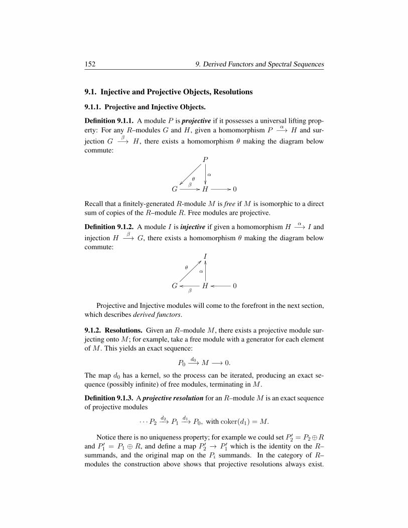
152 9. Derived Functors and Spectral Sequences
9.1. Injective and Projective Objects, Resolutions
9.1.1. Projective and Injective Objects.
Definition 9.1.1. A module P is projective if it possesses a universal lifting prop-erty: For any R–modules G and H , given a homomorphism P
α−→ H and sur-
jection Gβ−→ H , there exists a homomorphism θ making the diagram below
commute:P
θ~~
α
G
β // H // 0
Recall that a finitely-generated R-module M is free if M is isomorphic to a directsum of copies of the R–module R. Free modules are projective.
Definition 9.1.2. A module I is injective if given a homomorphism Hα−→ I and
injection Hβ−→ G, there exists a homomorphism θ making the diagram below
commute:I
G
θ
>>
H
α
OO
βoo 0oo
Projective and Injective modules will come to the forefront in the next section,which describes derived functors.
9.1.2. Resolutions. Given an R–module M , there exists a projective module sur-jecting onto M ; for example, take a free module with a generator for each elementof M . This yields an exact sequence:
P0d0−→M −→ 0.
The map d0 has a kernel, so the process can be iterated, producing an exact se-quence (possibly infinite) of free modules, terminating in M .
Definition 9.1.3. A projective resolution for anR–moduleM is an exact sequenceof projective modules
· · ·P2d2−→ P1
d1−→ P0, with coker(d1) = M.
Notice there is no uniqueness property; for example we could set P ′2 = P2⊕Rand P ′1 = P1 ⊕ R, and define a map P ′2 → P ′1 which is the identity on the R–summands, and the original map on the Pi summands. In the category of R–modules the construction above shows that projective resolutions always exist.
9.2. Derived Functors 153
Surprisingly this is not the case for sheaves of OX -modules. In fact ([90], ExerciseIII.6.2), for X = P1 there is no projective object surjecting onto OX .
Definition 9.1.4. An injective resolution for anR–moduleM is an exact sequenceof injective modules
I0d0−→ I1
d1−→ I2, · · · with ker(d0) = M.
It is not obvious that injective resolutions exist, but it can be shown (e.g. [70], [90],[149]) that in both the category of R–modules and in the category of sheaves ofOX–modules, every object does have an injective resolution.
Exercise 9.1.5. Prove that in the category of Z-modules (Abelian groups) thatevery object has an injective resolution. An injective Z-module is called divisible;if you get stuck, see §IV.3 of [93]. Exercise 9.1.6. Prove that in a category in which every object includes in an injec-tive object, injective resolutions of complexes always exist.
9.2. Derived Functors
In this section we describe the construction of derived functors, focusing on Exti
(in the category ofR-modules) andH i (in the category of sheaves of OX–modules).For brevity we call these two categories “our categories”. Working in our cate-gories keeps things concrete and lets us avoid introducing too much terminology,while highlighting the most salient features of the constructions, most of which ap-ply in much more general contexts. For proofs and a detailed discussion, see [70]or [149]. We quickly review the definitions from Chapter 7:
9.2.1. Categories and Functors. Recall that a category is a class of objects, alongwith morphisms between the objects, satisfying certain properties: composition ofmorphisms is associative, and identity morphisms exist.
Definition 9.2.1. Suppose B and C are categories. A functor F is a function fromB to C , taking objects to objects and morphisms to morphisms, preserving identitymorphisms and compositions. If
B1b1−→ B2
b2−→ B3
is a sequence of objects and morphisms in B, then
• F is covariant if applying F yields a sequence of objects and morphismsin C of the form:
F (B1)F (b1)−−−→ F (B2)
F (b2)−−−→ F (B3).
154 9. Derived Functors and Spectral Sequences
• F is contravariant if applying F yields a sequence of objects and mor-phisms in C of the form:
F (B3)F (b2)−−−→ F (B2)
F (b1)−−−→ F (B1).
A functor is additive if it preserves addition of homomorphisms; this propertywill be necessary in the construction of derived functors.
Example 9.2.2. The global sections functor of Chapter 3 is covariant: given asequence of OX–modules
M1f−→M2
g−→M3,
taking global sections yields a sequence
Γ(M1)→ Γ(M2)→ Γ(M3).
Definition 9.2.3. Let F be a functor from B to C , with B and C categories ofmodules over a ring. Let
0 // B1b1 // B2
b2 // B3// 0
be a short exact sequence. F is left–exact if either
(a) F is covariant, and the sequence
0 // F (B1)F (b1) // F (B2)
F (b2) // F (B3) is exact, or
(b) F is contravariant, and the sequence
0 // F (B3)F (b2) // F (B2)
F (b1) // F (B1) is exact.
A similar definition applies for right exactness; a functor F is said to be exact if itis both left and right exact, which means that F preserves exact sequences.
9.2.2. Constructing Derived Functors. The construction of derived functors ismotivated by the following question: if F is a left exact, contravariant functor and
0 // B1b1 // B2
b2 // B3// 0
is a short exact sequence, then what is the cokernel of F (b1)? This object willappear on the right of F (B1) in (b) above. A left exact functor has right derivedfunctors. Similarly, a right exact functor has left derived functors.
Definition 9.2.4. Let B be the category of modules over a ring, and let F be a leftexact, contravariant, additive functor from B to itself. If M ∈ B, then there existsa projective resolution P• for M .
· · · // P2d2 // P1
d1 // P0
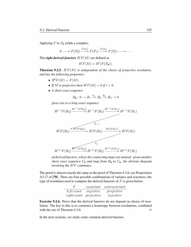
9.2. Derived Functors 155
Applying F to P• yields a complex:
0 // F (P0)F (d1) // F (P1)
F (d2) // F (P2) // · · · .
The right derived functors RiF (M) are defined as
RiF (M) = H i(F (P•)).
Theorem 9.2.5. RiF (M) is independent of the choice of projective resolution,and has the following properties:
• R0F (M) = F (M).
• If M is projective then RiF (M) = 0 if i > 0.
• A short exact sequence
B• : 0→ B1b1−→ B2
b2−→ B3 → 0
gives rise to a long exact sequence
Rj−1F (B3)Rj−1(F (b2))// Rj−1F (B2)
Rj−1(F (b1))// Rj−1F (B1)
δj−1
ttRjF (B3)
Rj(F (b2)) // RjF (B2)Rj(F (b1)) // RjF (B1)
δj
ttRj+1F (B3)
Rj+1(F (b2))// Rj+1F (B2)Rj+1(F (b1))// Rj+1F (B1)
of derived functors, where the connecting maps are natural: given anothershort exact sequence C• and map from B• to C•, the obvious diagraminvolving the RiF commutes.
The proof is almost exactly the same as the proof of Theorem 4.3.6; see PropositionA3.17 of [70]. There are four possible combinations of variance and exactness; thetype of resolution used to compute the derived functors of F is given below:
F covariant contravariant
left exact injective projectiveright exact projective injective
Exercise 9.2.6. Prove that the derived functors do not depend on choice of reso-lution. The key to this is to construct a homotopy between resolutions, combinedwith the use of Theorem 4.3.6. In the next sections, we study some common derived functors.
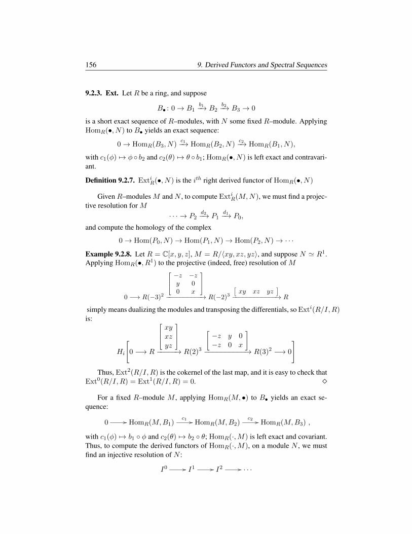
156 9. Derived Functors and Spectral Sequences
9.2.3. Ext. Let R be a ring, and suppose
B• : 0→ B1b1−→ B2
b2−→ B3 → 0
is a short exact sequence of R–modules, with N some fixed R–module. ApplyingHomR(•, N) to B• yields an exact sequence:
0→ HomR(B3, N)c1−→ HomR(B2, N)
c2−→ HomR(B1, N),
with c1(φ) 7→ φ b2 and c2(θ) 7→ θ b1; HomR(•, N) is left exact and contravari-ant.
Definition 9.2.7. ExtiR(•, N) is the ith right derived functor of HomR(•, N)
GivenR–modulesM andN , to compute ExtiR(M,N), we must find a projec-tive resolution for M
· · · → P2d2−→ P1
d1−→ P0,
and compute the homology of the complex
0→ Hom(P0, N)→ Hom(P1, N)→ Hom(P2, N)→ · · ·
Example 9.2.8. Let R = C[x, y, z], M = R/〈xy, xz, yz〉, and suppose N ' R1.Applying HomR(•, R1) to the projective (indeed, free) resolution of M
0 −→ R(−3)2
−z −zy 00 x
−−−−−−−−−−→ R(−2)3
[xy xz yz
]−−−−−−−−−−−−→ R
simply means dualizing the modules and transposing the differentials, so Exti(R/I,R)is:
Hi
[0 −→ R
xyxzyz
−−−−−→ R(2)3
−z y 0−z 0 x
−−−−−−−−−−→ R(3)2 −→ 0
]Thus, Ext2(R/I,R) is the cokernel of the last map, and it is easy to check that
Ext0(R/I,R) = Ext1(R/I,R) = 0. For a fixed R–module M , applying HomR(M, •) to B• yields an exact se-
quence:
0 // HomR(M,B1)c1 // HomR(M,B2)
c2 // HomR(M,B3) ,
with c1(φ) 7→ b1 φ and c2(θ) 7→ b2 θ; HomR(·,M) is left exact and covariant.Thus, to compute the derived functors of HomR(·,M), on a module N , we mustfind an injective resolution of N :
I0 // I1 // I2 // · · ·
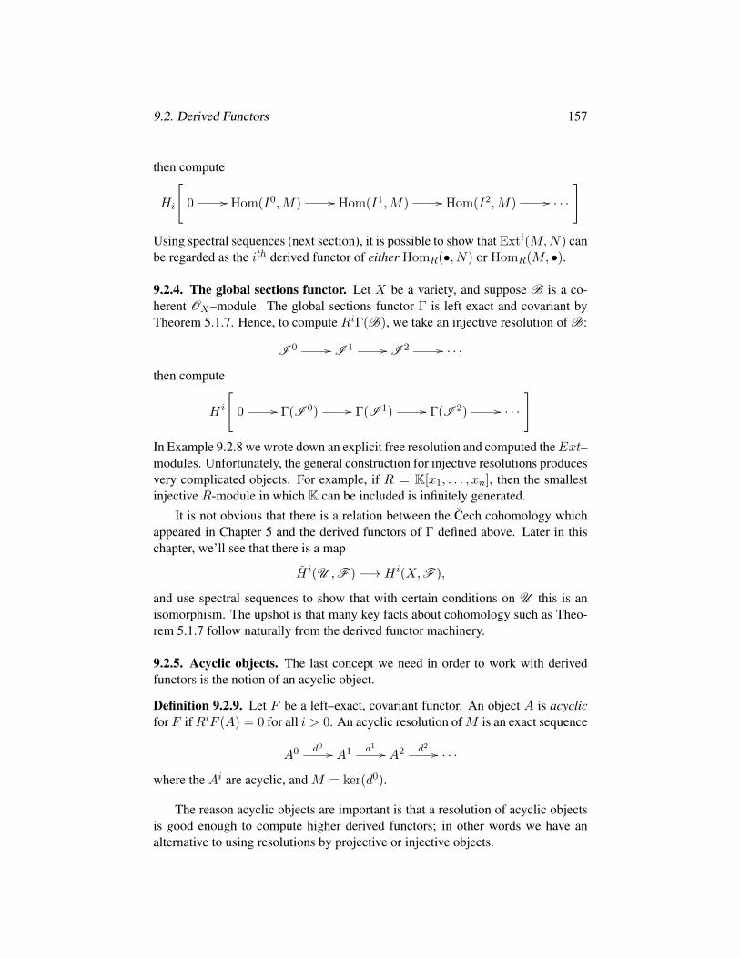
9.2. Derived Functors 157
then compute
Hi
[0 // Hom(I0,M) // Hom(I1,M) // Hom(I2,M) // · · ·
]Using spectral sequences (next section), it is possible to show that Exti(M,N) canbe regarded as the ith derived functor of either HomR(•, N) or HomR(M, •).
9.2.4. The global sections functor. Let X be a variety, and suppose B is a co-herent OX–module. The global sections functor Γ is left exact and covariant byTheorem 5.1.7. Hence, to compute RiΓ(B), we take an injective resolution of B:
I 0 // I 1 // I 2 // · · ·
then compute
H i
[0 // Γ(I 0) // Γ(I 1) // Γ(I 2) // · · ·
]In Example 9.2.8 we wrote down an explicit free resolution and computed theExt–modules. Unfortunately, the general construction for injective resolutions producesvery complicated objects. For example, if R = K[x1, . . . , xn], then the smallestinjective R-module in which K can be included is infinitely generated.
It is not obvious that there is a relation between the Cech cohomology whichappeared in Chapter 5 and the derived functors of Γ defined above. Later in thischapter, we’ll see that there is a map
H i(U ,F ) −→ H i(X,F ),
and use spectral sequences to show that with certain conditions on U this is anisomorphism. The upshot is that many key facts about cohomology such as Theo-rem 5.1.7 follow naturally from the derived functor machinery.
9.2.5. Acyclic objects. The last concept we need in order to work with derivedfunctors is the notion of an acyclic object.
Definition 9.2.9. Let F be a left–exact, covariant functor. An object A is acyclicfor F ifRiF (A) = 0 for all i > 0. An acyclic resolution ofM is an exact sequence
A0 d0// A1 d1
// A2 d2// · · ·
where the Ai are acyclic, and M = ker(d0).
The reason acyclic objects are important is that a resolution of acyclic objectsis good enough to compute higher derived functors; in other words we have analternative to using resolutions by projective or injective objects.
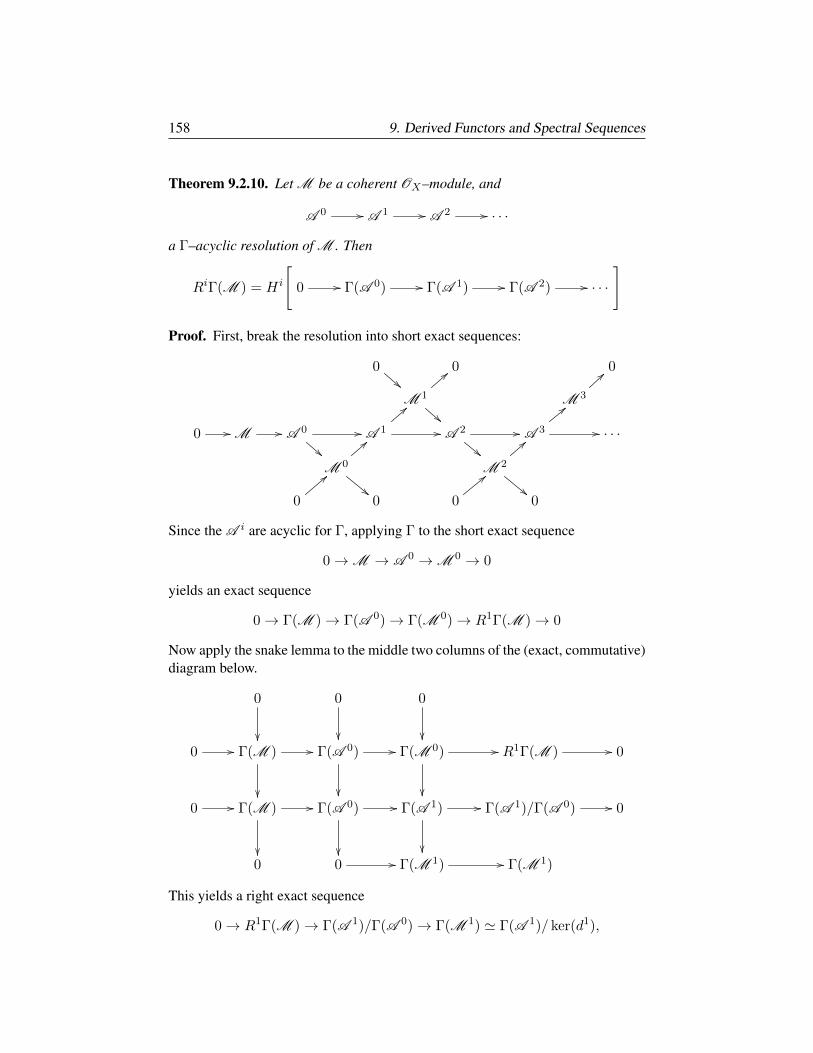
158 9. Derived Functors and Spectral Sequences
Theorem 9.2.10. Let M be a coherent OX–module, and
A 0 // A 1 // A 2 // · · ·
a Γ–acyclic resolution of M . Then
RiΓ(M ) = H i
[0 // Γ(A 0) // Γ(A 1) // Γ(A 2) // · · ·
]
Proof. First, break the resolution into short exact sequences:
0""
0 0
M 1
!!
<<
M 3
==
0 //M // A 0 //
!!A 1 //
==
A 2 //
!!A 3 //
==
· · ·
M 0
==
""
M 2
""
==
0
<<
0 0
<<
0
Since the A i are acyclic for Γ, applying Γ to the short exact sequence
0→M → A 0 →M 0 → 0
yields an exact sequence
0→ Γ(M )→ Γ(A 0)→ Γ(M 0)→ R1Γ(M )→ 0
Now apply the snake lemma to the middle two columns of the (exact, commutative)diagram below.
0
0
0
0 // Γ(M ) //
Γ(A 0) //
Γ(M 0) //
R1Γ(M ) // 0
0 // Γ(M ) //
Γ(A 0) //
Γ(A 1) //
Γ(A 1)/Γ(A 0) // 0
0 0 // Γ(M 1) // Γ(M 1)
This yields a right exact sequence
0→ R1Γ(M )→ Γ(A 1)/Γ(A 0)→ Γ(M 1) ' Γ(A 1)/ ker(d1),
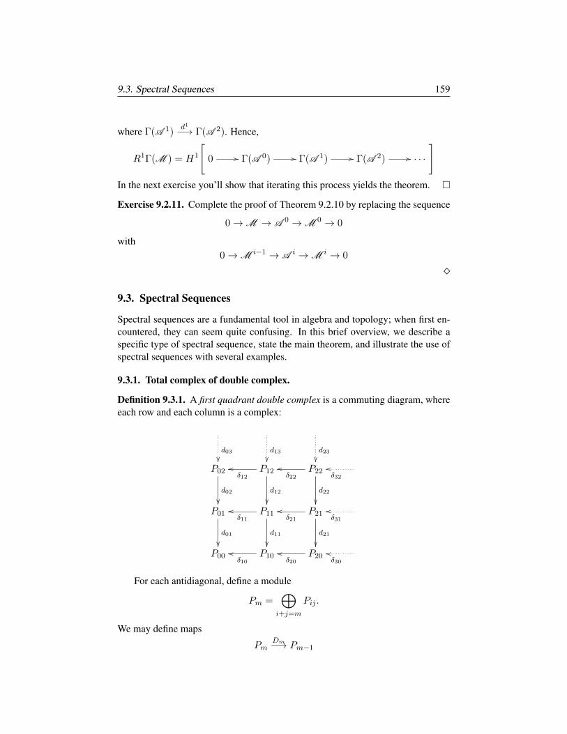
9.3. Spectral Sequences 159
where Γ(A 1)d1
−→ Γ(A 2). Hence,
R1Γ(M ) = H1
[0 // Γ(A 0) // Γ(A 1) // Γ(A 2) // · · ·
]In the next exercise you’ll show that iterating this process yields the theorem.
Exercise 9.2.11. Complete the proof of Theorem 9.2.10 by replacing the sequence
0→M → A 0 →M 0 → 0
with0→M i−1 → A i →M i → 0
9.3. Spectral Sequences
Spectral sequences are a fundamental tool in algebra and topology; when first en-countered, they can seem quite confusing. In this brief overview, we describe aspecific type of spectral sequence, state the main theorem, and illustrate the use ofspectral sequences with several examples.
9.3.1. Total complex of double complex.
Definition 9.3.1. A first quadrant double complex is a commuting diagram, whereeach row and each column is a complex:
d03
d13
d23
P02
d02
P12
d12
δ12
oo P22
d22
δ22
ooδ32
oo
P01
d01
P11
d11
δ11
oo P21
d21
δ21
ooδ31
oo
P00 P10δ10
oo P20δ20
ooδ30
oo
For each antidiagonal, define a module
Pm =⊕i+j=m
Pij .
We may define maps
PmDm−→ Pm−1
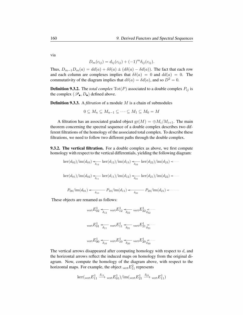
160 9. Derived Functors and Spectral Sequences
via
Dm(cij) = dij(cij) + (−1)mδij(cij).
Thus, Dm−1Dm(a) = dd(a) + δδ(a) ± (dδ(a) − δd(a)). The fact that each rowand each column are complexes implies that δδ(a) = 0 and dd(a) = 0. Thecommutativity of the diagram implies that dδ(a) = δd(a), and so D2 = 0.
Definition 9.3.2. The total complex Tot(P ) associated to a double complex Pij isthe complex (P•, D•) defined above.
Definition 9.3.3. A filtration of a module M is a chain of submodules
0 ⊆Mn ⊆Mn−1 ⊆ · · · ⊆M1 ⊆M0 = M
A filtration has an associated graded object gr(M) = ⊕Mi/Mi+1. The maintheorem concerning the spectral sequence of a double complex describes two dif-ferent filtrations of the homology of the associated total complex. To describe thesefiltrations, we need to follow two different paths through the double complex.
9.3.2. The vertical filtration. For a double complex as above, we first computehomology with respect to the vertical differentials, yielding the following diagram:
ker(d02)/im(d03) ker(d12)/im(d13)δ12
oo ker(d22)/im(d23)δ22
oo oo
ker(d01)/im(d02) ker(d11)/im(d12)δ11
oo ker(d21)/im(d22)δ21
oo oo
P00/im(d01) P10/im(d11)δ10
oo P20/im(d21)δ20
oo oo
These objects are renamed as follows:
vertE102 vertE
112δ12
oovertE
122δ22
ooδ32
oo
vertE101 vertE
111δ11
oovertE
121δ21
ooδ31
oo
vertE100 vertE
110δ10
oovertE
120δ20
ooδ30
oo
The vertical arrows disappeared after computing homology with respect to d, andthe horizontal arrows reflect the induced maps on homology from the original di-agram. Now, compute the homology of the diagram above, with respect to thehorizontal maps. For example, the object vertE
211 represents
ker(vertE111
δ11−→ vertE101)/im(vertE
121
δ21−→ vertE111)
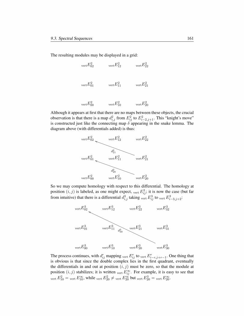
9.3. Spectral Sequences 161
The resulting modules may be displayed in a grid:
vertE202 vertE
212 vertE
222
vertE201 vertE
211 vertE
221
vertE200 vertE
210 vertE
220
Although it appears at first that there are no maps between these objects, the crucialobservation is that there is a map d2
i,j from E2ij to E2
i−2,j+1. This “knight’s move”is constructed just like the connecting map δ appearing in the snake lemma. Thediagram above (with differentials added) is thus:
vertE202 vertE
212 vertE
222
vertE201 vertE
211 vertE
221
d221
ii
vertE200 vertE
210 vertE
220
d220
ii
So we may compute homology with respect to this differential. The homology atposition (i, j) is labeled, as one might expect, vertE
3ij ; it is now the case (but far
from intuitive) that there is a differential d3i,j taking vertE
3ij to vertE
3i−3,j+2:
vertE302 vertE
312 vertE
322 vertE
332
vertE301 vertE
311 vertE
321 vertE
331
vertE300 vertE
310 vertE
320 vertE
330
d330
gg
The process continues, with drij mapping vertErij to vertE
ri−r,j+r−1. One thing that
is obvious is that since the double complex lies in the first quadrant, eventuallythe differentials in and out at position (i, j) must be zero, so that the module atposition (i, j) stabilizes; it is written vertE
∞ij . For example, it is easy to see that
vertE210 = vertE
∞10 , while vertE
220 6= vertE
∞20 but vertE
320 = vertE
∞20 .
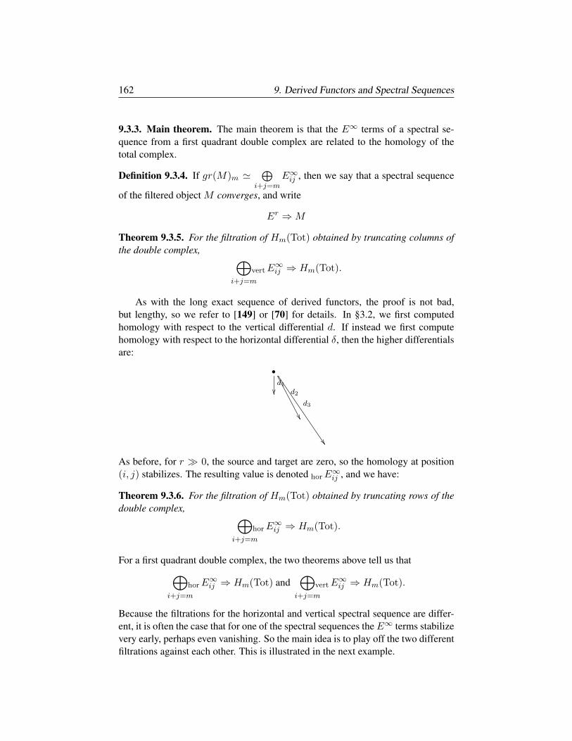
162 9. Derived Functors and Spectral Sequences
9.3.3. Main theorem. The main theorem is that the E∞ terms of a spectral se-quence from a first quadrant double complex are related to the homology of thetotal complex.
Definition 9.3.4. If gr(M)m '⊕
i+j=mE∞ij , then we say that a spectral sequence
of the filtered object M converges, and write
Er ⇒M
Theorem 9.3.5. For the filtration of Hm(Tot) obtained by truncating columns ofthe double complex, ⊕
i+j=m
vertE∞ij ⇒ Hm(Tot).
As with the long exact sequence of derived functors, the proof is not bad,but lengthy, so we refer to [149] or [70] for details. In §3.2, we first computedhomology with respect to the vertical differential d. If instead we first computehomology with respect to the horizontal differential δ, then the higher differentialsare:
•d1
d2
d3
As before, for r 0, the source and target are zero, so the homology at position(i, j) stabilizes. The resulting value is denoted horE
∞ij , and we have:
Theorem 9.3.6. For the filtration of Hm(Tot) obtained by truncating rows of thedouble complex, ⊕
i+j=m
horE∞ij ⇒ Hm(Tot).
For a first quadrant double complex, the two theorems above tell us that⊕i+j=m
horE∞ij ⇒ Hm(Tot) and
⊕i+j=m
vertE∞ij ⇒ Hm(Tot).
Because the filtrations for the horizontal and vertical spectral sequence are differ-ent, it is often the case that for one of the spectral sequences theE∞ terms stabilizevery early, perhaps even vanishing. So the main idea is to play off the two differentfiltrations against each other. This is illustrated in the next example.
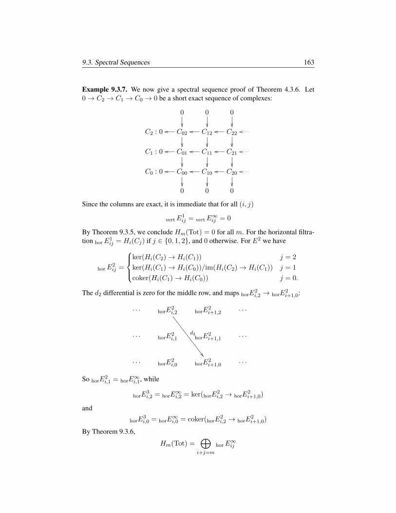
9.3. Spectral Sequences 163
Example 9.3.7. We now give a spectral sequence proof of Theorem 4.3.6. Let0→ C2 → C1 → C0 → 0 be a short exact sequence of complexes:
0
0
0
C2 : 0 C02
oo C12
oo C22
oo oo
C1 : 0 C01
oo C11
oo C21
oo oo
C0 : 0 C00oo
C10
oo C20oo
oo
0 0 0
Since the columns are exact, it is immediate that for all (i, j)
vertE1ij = vertE
∞ij = 0
By Theorem 9.3.5, we conclude Hm(Tot) = 0 for all m. For the horizontal filtra-tion horE
1ij = Hi(Cj) if j ∈ 0, 1, 2, and 0 otherwise. For E2 we have
horE2ij =
ker(Hi(C2)→ Hi(C1)) j = 2
ker(Hi(C1)→ Hi(C0))/im(Hi(C2)→ Hi(C1)) j = 1
coker(Hi(C1)→ Hi(C0)) j = 0.
The d2 differential is zero for the middle row, and maps horE2i,2 → horE
2i+1,0:
· · · horE2i,2
d2
horE2i+1,2 · · ·
· · · horE2i,1 horE
2i+1,1 · · ·
· · · horE2i,0 horE
2i+1,0 · · ·
So horE2i,1 = horE
∞i,1, while
horE3i,2 = horE
∞i,2 = ker(horE
2i,2 → horE
2i+1,0)
and
horE3i,0 = horE
∞i,0 = coker(horE
2i,2 → horE
2i+1,0)
By Theorem 9.3.6,
Hm(Tot) =⊕i+j=m
horE∞ij
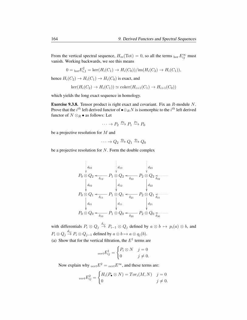
164 9. Derived Functors and Spectral Sequences
From the vertical spectral sequence, Hm(Tot) = 0, so all the terms horE∞ij must
vanish. Working backwards, we see this means
0 = horE2i,1 = ker(Hi(C1)→ Hi(C0))/im(Hi(C2)→ Hi(C1)),
hence Hi(C2)→ Hi(C1)→ Hi(C0) is exact, and
ker(Hi(C2)→ Hi(C1)) ' coker(Hi+1(C1)→ Hi+1(C0))
which yields the long exact sequence in homology.
Exercise 9.3.8. Tensor product is right exact and covariant. Fix an R-module N .Prove that the ith left derived functor of •⊗RN is isomorphic to the ith left derivedfunctor of N ⊗R • as follows: Let
· · · → P2p2−→ P1
p1−→ P0
be a projective resolution for M and
· · · → Q2q2−→ Q1
q1−→ Q0
be a projective resolution for N . Form the double complex
d03
d13
d23
P0 ⊗Q2
d02
P1 ⊗Q2
d12
δ12
oo P2 ⊗Q2
d22
δ22
ooδ32
oo
P0 ⊗Q1
d01
P1 ⊗Q1
d11
δ11
oo P2 ⊗Q1
d21
δ21
ooδ31
oo
P0 ⊗Q0 P1 ⊗Q0δ10
oo P2 ⊗Q0δ20
ooδ30
oo
with differentials Pi ⊗ Qjδij→ Pi−1 ⊗ Qj defined by a ⊗ b 7→ pi(a) ⊗ b, and
Pi ⊗Qjdij→ Pi ⊗Qj−1 defined by a⊗ b 7→ a⊗ qj(b).
(a) Show that for the vertical filtration, the E1 terms are
vertE1ij =
Pi ⊗N j = 0
0 j 6= 0.
Now explain why vertE2 = vertE
∞, and these terms are:
vertE2ij =
Hi(P• ⊗N) = Tori(M,N) j = 0
0 j 6= 0.
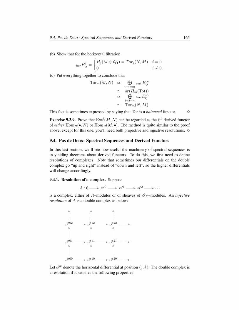
9.4. Pas de Deux: Spectral Sequences and Derived Functors 165
(b) Show that for the horizontal filtration
horE2ij =
Hj(M ⊗Q•) = Torj(N,M) i = 0
0 i 6= 0.
(c) Put everything together to conclude that
Torm(M,N) '⊕
i+j=mvertE
∞ij
' gr(Hm(Tot))'
⊕i+j=m
horE∞ij
' Torm(N,M)
This fact is sometimes expressed by saying that Tor is a balanced functor. Exercise 9.3.9. Prove that Exti(M,N) can be regarded as the ith derived functorof either HomR(•, N) or HomR(M, •). The method is quite similar to the proofabove, except for this one, you’ll need both projective and injective resolutions.
9.4. Pas de Deux: Spectral Sequences and Derived Functors
In this last section, we’ll see how useful the machinery of spectral sequences isin yielding theorems about derived functors. To do this, we first need to defineresolutions of complexes. Note that sometimes our differentials on the doublecomplex go “up and right” instead of “down and left”, so the higher differentialswill change accordingly.
9.4.1. Resolution of a complex. Suppose
A : 0 // A 0 // A 1 // A 2 // · · ·
is a complex, either of R–modules or of sheaves of OX–modules. An injectiveresolution of A is a double complex as below:
I 02 //
OO
I 12
OO
// I 22
OO
//
I 01
OO
// I 11
OO
// I 21
OO
//
I 00 //
OO
I 10 //
OO
I 20 //
OO
Let djk denote the horizontal differential at position (j, k). The double complex isa resolution if it satisfies the following properties
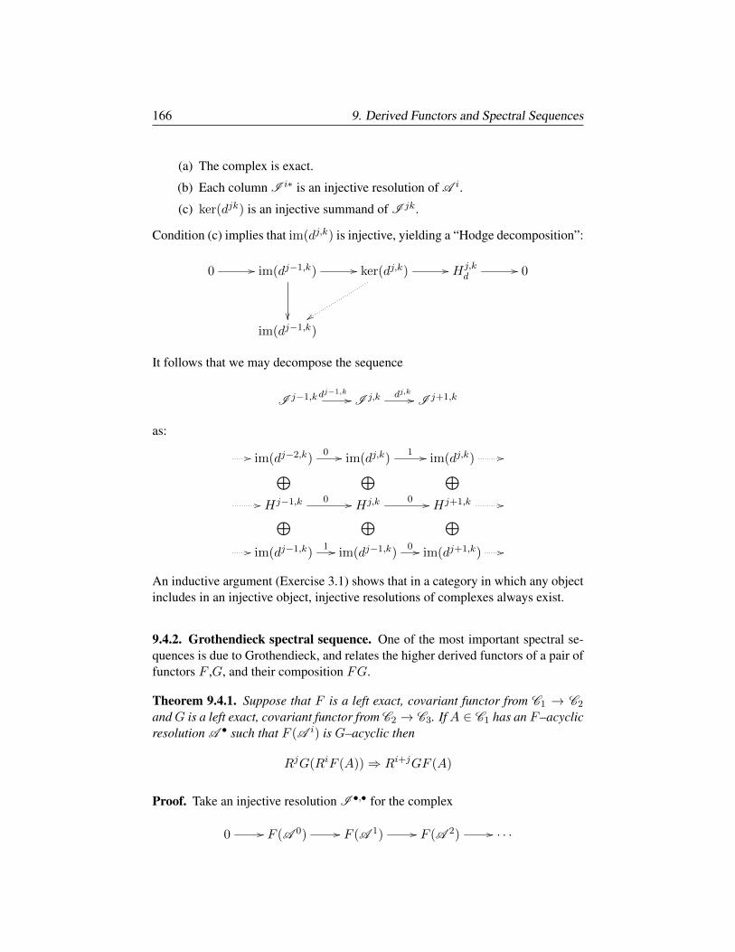
166 9. Derived Functors and Spectral Sequences
(a) The complex is exact.
(b) Each column I i∗ is an injective resolution of A i.
(c) ker(djk) is an injective summand of I jk.
Condition (c) implies that im(dj,k) is injective, yielding a “Hodge decomposition”:
0 // im(dj−1,k) //
ker(dj,k) //
yy
Hj,kd
// 0
im(dj−1,k)
It follows that we may decompose the sequence
I j−1,k dj−1,k
// I j,k dj,k // I j+1,k
as:
// im(dj−2,k)0 // im(dj,k)
1 // im(dj,k) //⊕ ⊕ ⊕// Hj−1,k 0 // Hj,k 0 // Hj+1,k //⊕ ⊕ ⊕// im(dj−1,k)
1 // im(dj−1,k)0 // im(dj+1,k) //
An inductive argument (Exercise 3.1) shows that in a category in which any objectincludes in an injective object, injective resolutions of complexes always exist.
9.4.2. Grothendieck spectral sequence. One of the most important spectral se-quences is due to Grothendieck, and relates the higher derived functors of a pair offunctors F ,G, and their composition FG.
Theorem 9.4.1. Suppose that F is a left exact, covariant functor from C1 → C2
andG is a left exact, covariant functor from C2 → C3. IfA ∈ C1 has an F–acyclicresolution A • such that F (A i) is G–acyclic then
RjG(RiF (A))⇒ Ri+jGF (A)
Proof. Take an injective resolution I •,• for the complex
0 // F (A 0) // F (A 1) // F (A 2) // · · ·
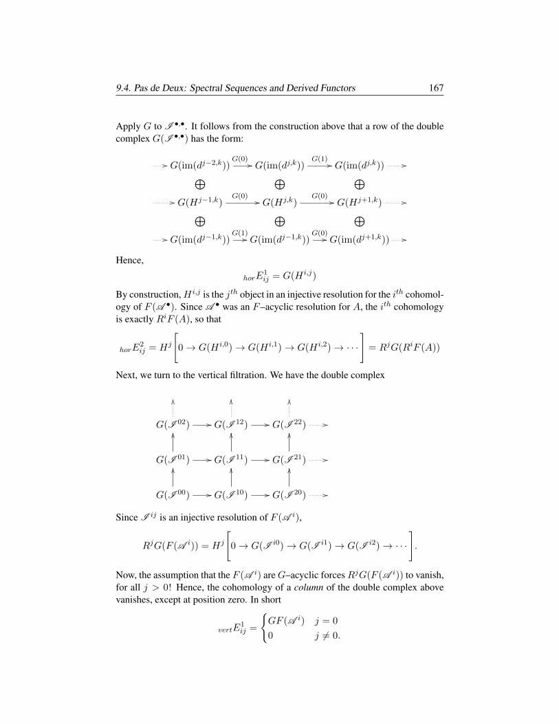
9.4. Pas de Deux: Spectral Sequences and Derived Functors 167
Apply G to I •,•. It follows from the construction above that a row of the doublecomplex G(I •,•) has the form:
// G(im(dj−2,k))G(0) // G(im(dj,k))
G(1) // G(im(dj,k)) //⊕ ⊕ ⊕// G(Hj−1,k)
G(0) // G(Hj,k)G(0) // G(Hj+1,k) //⊕ ⊕ ⊕
// G(im(dj−1,k))G(1)// G(im(dj−1,k))
G(0)// G(im(dj+1,k)) //
Hence,
horE1ij = G(H i,j)
By construction,H i,j is the jth object in an injective resolution for the ith cohomol-ogy of F (A •). Since A • was an F–acyclic resolution for A, the ith cohomologyis exactly RiF (A), so that
horE2ij = Hj
[0→ G(H i,0)→ G(H i,1)→ G(H i,2)→ · · ·
]= RjG(RiF (A))
Next, we turn to the vertical filtration. We have the double complex
G(I 02) //
OO
G(I 12)
OO
// G(I 22)
OO
//
G(I 01)
OO
// G(I 11)
OO
// G(I 21)
OO
//
G(I 00) //
OO
G(I 10) //
OO
G(I 20) //
OO
Since I ij is an injective resolution of F (A i),
RjG(F (A i)) = Hj
[0→ G(I i0)→ G(I i1)→ G(I i2)→ · · ·
].
Now, the assumption that the F (A i) areG–acyclic forcesRjG(F (A i)) to vanish,for all j > 0! Hence, the cohomology of a column of the double complex abovevanishes, except at position zero. In short
vertE1ij =
GF (A i) j = 0
0 j 6= 0.
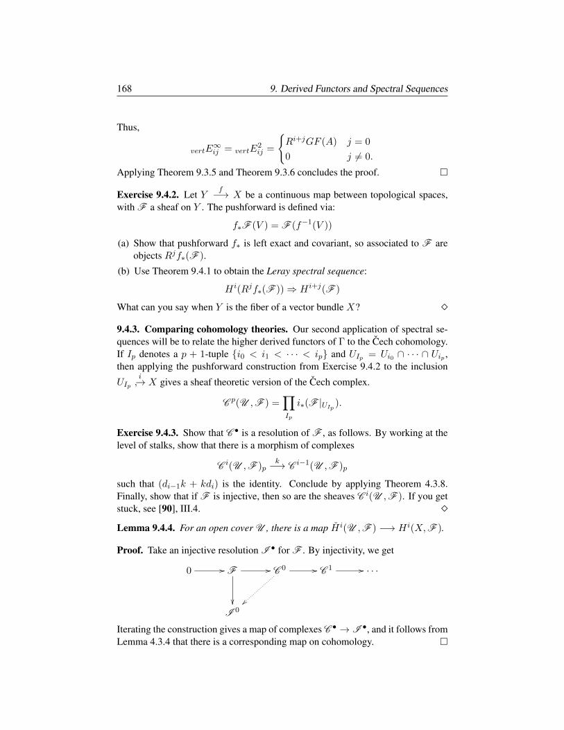
168 9. Derived Functors and Spectral Sequences
Thus,
vertE∞ij = vertE
2ij =
Ri+jGF (A) j = 0
0 j 6= 0.
Applying Theorem 9.3.5 and Theorem 9.3.6 concludes the proof.
Exercise 9.4.2. Let Yf−→ X be a continuous map between topological spaces,
with F a sheaf on Y . The pushforward is defined via:
f∗F (V ) = F (f−1(V ))
(a) Show that pushforward f∗ is left exact and covariant, so associated to F areobjects Rjf∗(F ).
(b) Use Theorem 9.4.1 to obtain the Leray spectral sequence:
H i(Rjf∗(F ))⇒ H i+j(F )
What can you say when Y is the fiber of a vector bundle X? 9.4.3. Comparing cohomology theories. Our second application of spectral se-quences will be to relate the higher derived functors of Γ to the Cech cohomology.If Ip denotes a p + 1-tuple i0 < i1 < · · · < ip and UIp = Ui0 ∩ · · · ∩ Uip ,then applying the pushforward construction from Exercise 9.4.2 to the inclusion
UIpi→ X gives a sheaf theoretic version of the Cech complex.
C p(U ,F ) =∏Ip
i∗(F |UIp ).
Exercise 9.4.3. Show that C • is a resolution of F , as follows. By working at thelevel of stalks, show that there is a morphism of complexes
C i(U ,F )pk−→ C i−1(U ,F )p
such that (di−1k + kdi) is the identity. Conclude by applying Theorem 4.3.8.Finally, show that if F is injective, then so are the sheaves C i(U ,F ). If you getstuck, see [90], III.4. Lemma 9.4.4. For an open cover U , there is a map H i(U ,F ) −→ H i(X,F ).
Proof. Take an injective resolution I • for F . By injectivity, we get
0 // F //
C 0 //
C 1 // · · ·
I 0
Iterating the construction gives a map of complexes C • → I •, and it follows fromLemma 4.3.4 that there is a corresponding map on cohomology.
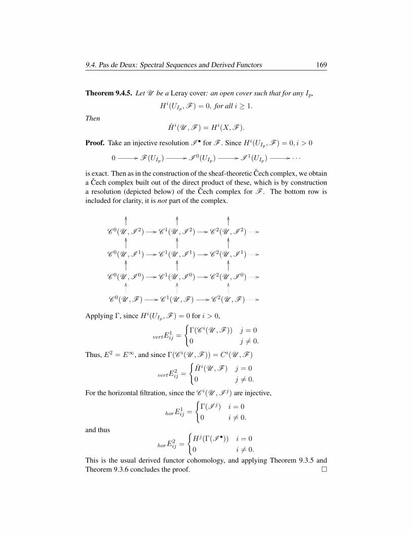
9.4. Pas de Deux: Spectral Sequences and Derived Functors 169
Theorem 9.4.5. Let U be a Leray cover: an open cover such that for any Ip,
H i(UIp ,F ) = 0, for all i ≥ 1.
ThenH i(U ,F ) = H i(X,F ).
Proof. Take an injective resolution I • for F . Since H i(UIp ,F ) = 0, i > 0
0 // F (UIp) // I 0(UIp) // I 1(UIp) // · · ·
is exact. Then as in the construction of the sheaf-theoretic Cech complex, we obtaina Cech complex built out of the direct product of these, which is by constructiona resolution (depicted below) of the Cech complex for F . The bottom row isincluded for clarity, it is not part of the complex.
C 0(U ,I 2) //
OO
C 1(U ,I 2) //
OO
C 2(U ,I 2) //
OO
C 0(U ,I 1) //
OO
C 1(U ,I 1) //
OO
C 2(U ,I 1) //
OO
C 0(U ,I 0) //
OO
C 1(U ,I 0) //
OO
C 2(U ,I 0) //
OO
C 0(U ,F ) //
OO
C 1(U ,F ) //
OO
C 2(U ,F ) //
OO
Applying Γ, since H i(UIp ,F ) = 0 for i > 0,
vertE1ij =
Γ(C i(U ,F )) j = 0
0 j 6= 0.
Thus, E2 = E∞, and since Γ(C i(U ,F )) = Ci(U ,F )
vertE2ij =
H i(U ,F ) j = 0
0 j 6= 0.
For the horizontal filtration, since the C i(U ,I j) are injective,
horE1ij =
Γ(I j) i = 0
0 i 6= 0.
and thus
horE2ij =
Hj(Γ(I •)) i = 0
0 i 6= 0.
This is the usual derived functor cohomology, and applying Theorem 9.3.5 andTheorem 9.3.6 concludes the proof.

170 9. Derived Functors and Spectral Sequences
9.4.4. Cartan–Eilenberg Resolution. A Cartan–Eilenberg resolution of a com-plex is a resolution constructed in a fashion similar to the injective resolution of acomplex appearing in §9.4.1. For a complex C•, take free resolutions Fi+1,• forim(∂i+1) and Gi,• for Hi(C). The short exact sequence
0 −→ im(∂i+1) −→ ker(∂i) −→ Hi(C) −→ 0
combined with the resolutions above yields a resolution Gi,• ⊕ Fi+1,• for ker(∂i).Now use the resolutions for ker(∂i) and im(∂i) and the short exact sequence
0 −→ ker(∂i) −→ Ci −→ im(∂i) −→ 0
to obtain a resolution for Ci. The resulting double complex has terms
Fi+1,j ⊕Gi,j ⊕ Fi,jdi,j−→ Fi,j ⊕Gi−1,j ⊕ Fi−1,j
with di,j the identity on Fi,j and zero on the other summands.
Example 9.4.6. Our final spectral sequence example comes from the three-parameterfiltration of S2 appearing in Example 8.4.3
with edges in degrees
ab = 001 ac = 011 ad = 001 bc = 010 bd = 100 cd = 010
and triangles in degrees
abc = 011 abd = 101 acd = 011 bcd = 110.
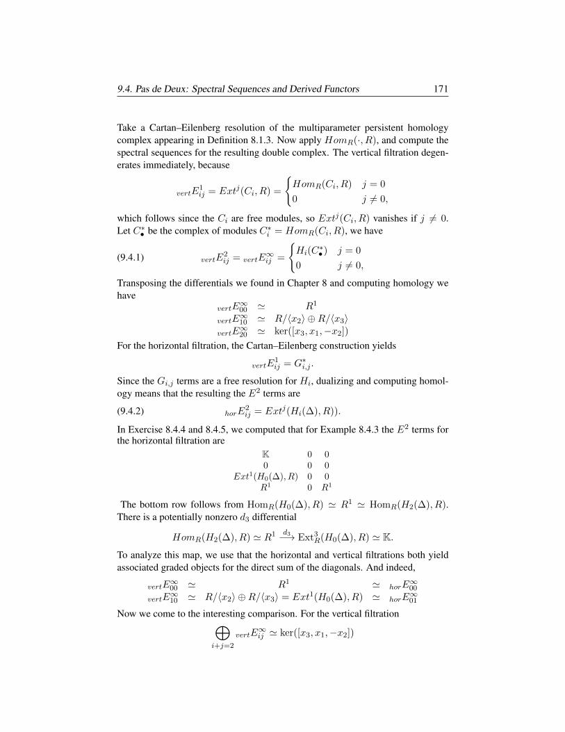
9.4. Pas de Deux: Spectral Sequences and Derived Functors 171
Take a Cartan–Eilenberg resolution of the multiparameter persistent homologycomplex appearing in Definition 8.1.3. Now apply HomR(·, R), and compute thespectral sequences for the resulting double complex. The vertical filtration degen-erates immediately, because
vertE1ij = Extj(Ci, R) =
HomR(Ci, R) j = 0
0 j 6= 0,
which follows since the Ci are free modules, so Extj(Ci, R) vanishes if j 6= 0.Let C∗• be the complex of modules C∗i = HomR(Ci, R), we have
(9.4.1) vertE2ij = vertE
∞ij =
Hi(C
∗• ) j = 0
0 j 6= 0,
Transposing the differentials we found in Chapter 8 and computing homology wehave
vertE∞00 ' R1
vertE∞10 ' R/〈x2〉 ⊕R/〈x3〉
vertE∞20 ' ker([x3, x1,−x2])
For the horizontal filtration, the Cartan–Eilenberg construction yields
vertE1ij = G∗i,j .
Since the Gi,j terms are a free resolution for Hi, dualizing and computing homol-ogy means that the resulting the E2 terms are
(9.4.2) horE2ij = Extj(Hi(∆), R)).
In Exercise 8.4.4 and 8.4.5, we computed that for Example 8.4.3 the E2 terms forthe horizontal filtration are
K 0 00 0 0
Ext1(H0(∆), R) 0 0R1 0 R1
The bottom row follows from HomR(H0(∆), R) ' R1 ' HomR(H2(∆), R).There is a potentially nonzero d3 differential
HomR(H2(∆), R) ' R1 d3−→ Ext3R(H0(∆), R) ' K.
To analyze this map, we use that the horizontal and vertical filtrations both yieldassociated graded objects for the direct sum of the diagonals. And indeed,
vertE∞00 ' R1 ' horE
∞00
vertE∞10 ' R/〈x2〉 ⊕R/〈x3〉 = Ext1(H0(∆), R) ' horE
∞01
Now we come to the interesting comparison. For the vertical filtration⊕i+j=2
vertE∞ij ' ker([x3, x1,−x2])
172 9. Derived Functors and Spectral Sequences
But this must be the associated graded of a filtration for H2(Tot). On the otherhand, ⊕
i+j=2
horE∞ij ' ker(d3)
So this means that we have a nontrivial d3 differential mapping
R1 → K = R1/〈x1, x2, x3〉,yielding
ker(d3) = ker([x3, x1,−x2])
By Theorem 8.4.1 the modules Extj(Hi(∆), R) encode the codimension j supportlocus of Hi(∆). This means they provide a natural way to stratify MPH modules.
The Hilbert Syzygy Theorem shows that the resolution for a K[x1, . . . , xn]-modulehas length at most n, so
Extj(Hi(∆), R) = 0
when j ≥ n+ 1. Combining this with Equations 9.4.1 and 9.4.2 proves
Theorem 9.4.7. For a Cartan–Eilenberg resolution of the MPH complex C• ofDefinition 8.1.3, we have ⊕
i+j=k
horE∞ij =⇒ Hk(C
∗• ),
andhorE
mij = horE
∞ij for all m ≥ n+ 1.
Exercise 9.4.8. Carry out this analysis for other examples. Notice for a filtrationwith r−parameters, Extj(Hi(∆), R) vanishes for j > r, which means that for thehorizontal filtration the differentials dj vanish for j > r.
Appendix A
Examples of SoftwarePackages
We include some examples of various software packages that perform the compu-tations discussed in this book. Software is dynamic, so at some point the syntaxfor the examples below will be outdated. Nevertheless, the general structure of thecomputations is illustrative, and worth including.
A.1. Covariance and spread of data via R
We begin with a “barehanded” approach: in Exercise 1.3.10, we considered thedataset
X = (1, 1), (2, 2), (2, 3), (3, 2), (3, 3), (4, 4)We found the covariance matrix, and computed the eigenvalues and eigenvectors.To visualize the ellipse that best fits the data, we use a standard statistics package:R, which is public domain, available athttps://www.r-project.org
# next commands load the visualization packagelibrary(ggplot2)library(ggpubr)
# next commands input data; if large data set load from filex = c(1, 2, 2, 3, 3, 4)y = c(1, 2, 3, 2, 3, 4)
datum = cbind(x, y)datum = as.data.frame(datum)
# next commands get the covariance matrix# note: without the second line, the result will not display
173
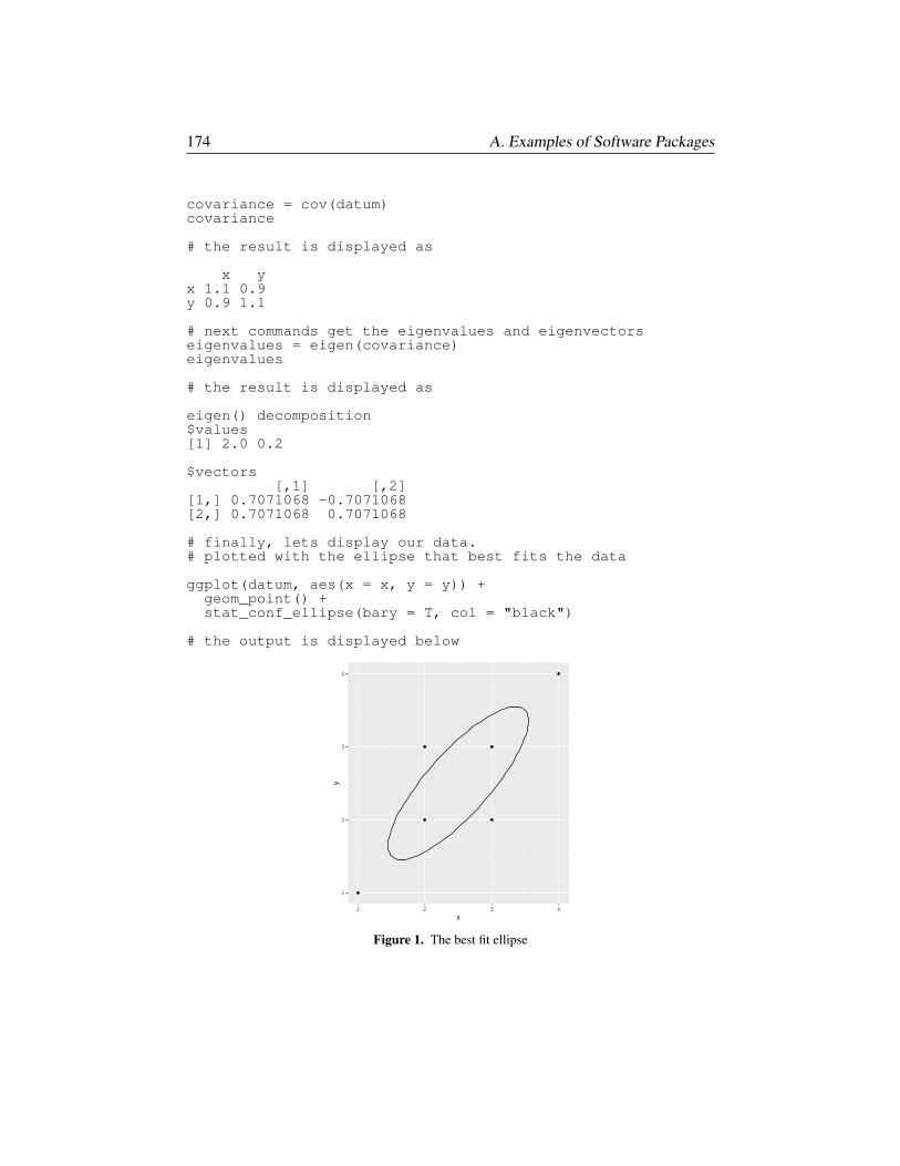
174 A. Examples of Software Packages
covariance = cov(datum)covariance
# the result is displayed as
x yx 1.1 0.9y 0.9 1.1
# next commands get the eigenvalues and eigenvectorseigenvalues = eigen(covariance)eigenvalues
# the result is displayed as
eigen() decomposition$values[1] 2.0 0.2
$vectors[,1] [,2]
[1,] 0.7071068 -0.7071068[2,] 0.7071068 0.7071068
# finally, lets display our data.# plotted with the ellipse that best fits the data
ggplot(datum, aes(x = x, y = y)) +geom_point() +stat_conf_ellipse(bary = T, col = "black")
# the output is displayed below
1
2
3
4
1 2 3 4x
y
Figure 1. The best fit ellipse
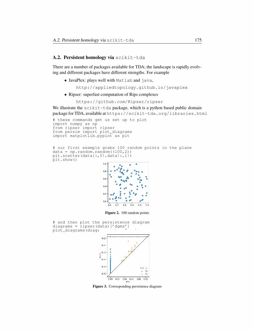
A.2. Persistent homology via scikit-tda 175
A.2. Persistent homology via scikit-tda
There are a number of packages available for TDA; the landscape is rapidly evolv-ing and different packages have different strengths. For example
• JavaPlex: plays well with Matlab and java,
http://appliedtopology.github.io/javaplex
• Ripser: superfast computation of Rips complexes
https://github.com/Ripser/ripser
We illustrate the scikit-tda package, which is a python based public domainpackage for TDA, available at https://scikit-tda.org/libraries.html# these commands get us set up to plotimport numpy as npfrom ripser import ripserfrom persim import plot_diagramsimport matplotlib.pyplot as plt
# our first example grabs 100 random points in the planedata = np.random.random((100,2))plt.scatter(data[:,0],data[:,1])plt.show()
Figure 2. 100 random points
# and then plot the persistence diagramdiagrams = ripser(data)[’dgms’]plot_diagrams(diagrams, show=True)
Figure 3. Corresponding persistence diagram
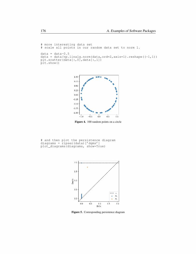
176 A. Examples of Software Packages
# more interesting data set# scale all points in our random data set to norm 1.
data = data-0.5data = data/np.linalg.norm(data,ord=2,axis=1).reshape((-1,1))plt.scatter(data[:,0],data[:,1])plt.show()
Figure 4. 100 random points on a circle
# and then plot the persistence diagramdiagrams = ripser(data)[’dgms’]plot_diagrams(diagrams, show=True)
Figure 5. Corresponding persistence diagram
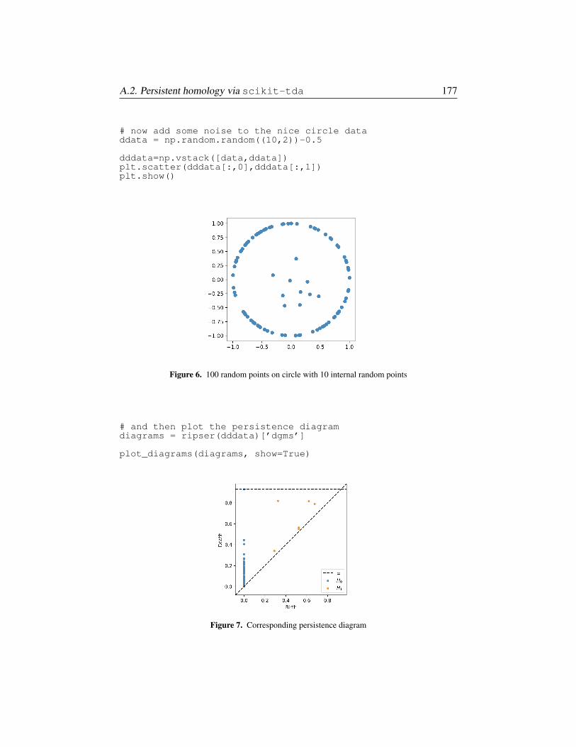
A.2. Persistent homology via scikit-tda 177
# now add some noise to the nice circle dataddata = np.random.random((10,2))-0.5
dddata=np.vstack([data,ddata])plt.scatter(dddata[:,0],dddata[:,1])plt.show()
Figure 6. 100 random points on circle with 10 internal random points
# and then plot the persistence diagramdiagrams = ripser(dddata)[’dgms’]
plot_diagrams(diagrams, show=True)
Figure 7. Corresponding persistence diagram
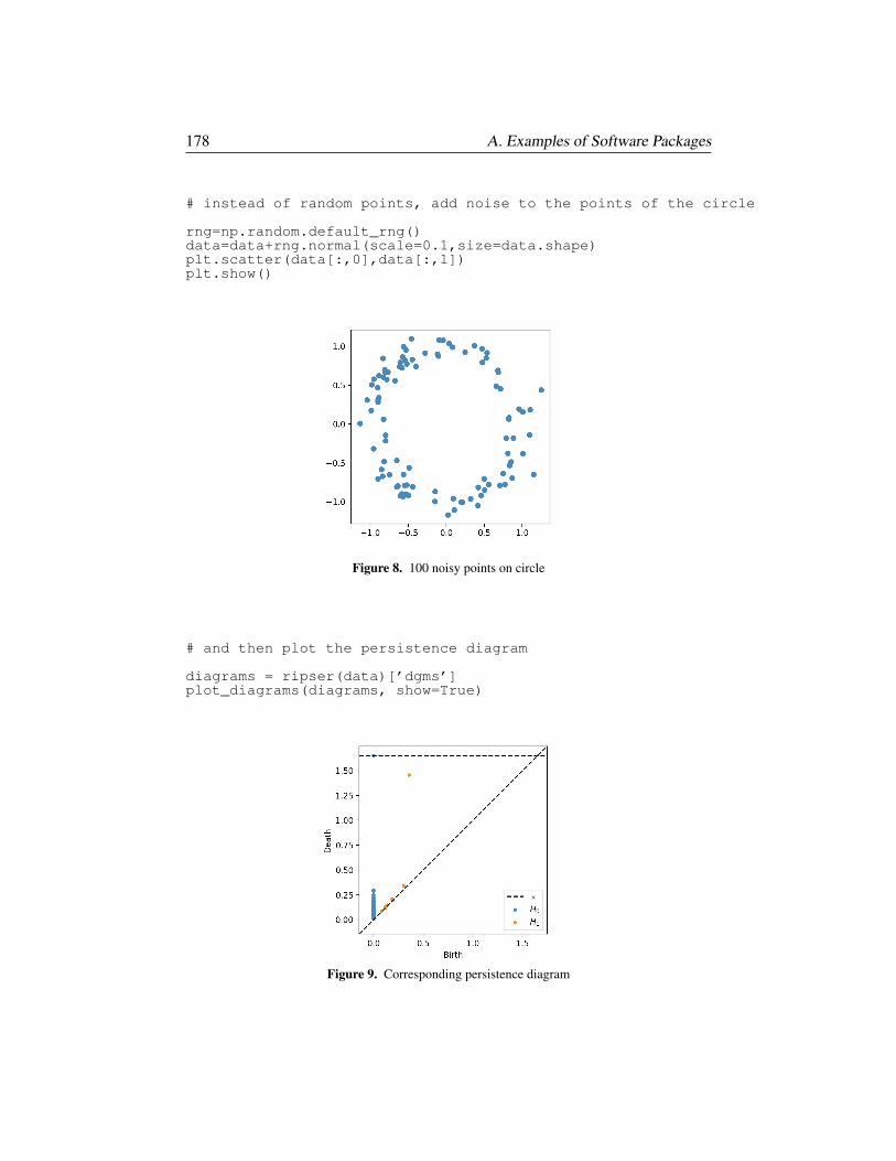
178 A. Examples of Software Packages
# instead of random points, add noise to the points of the circle
rng=np.random.default_rng()data=data+rng.normal(scale=0.1,size=data.shape)plt.scatter(data[:,0],data[:,1])plt.show()
Figure 8. 100 noisy points on circle
# and then plot the persistence diagram
diagrams = ripser(data)[’dgms’]plot_diagrams(diagrams, show=True)
Figure 9. Corresponding persistence diagram
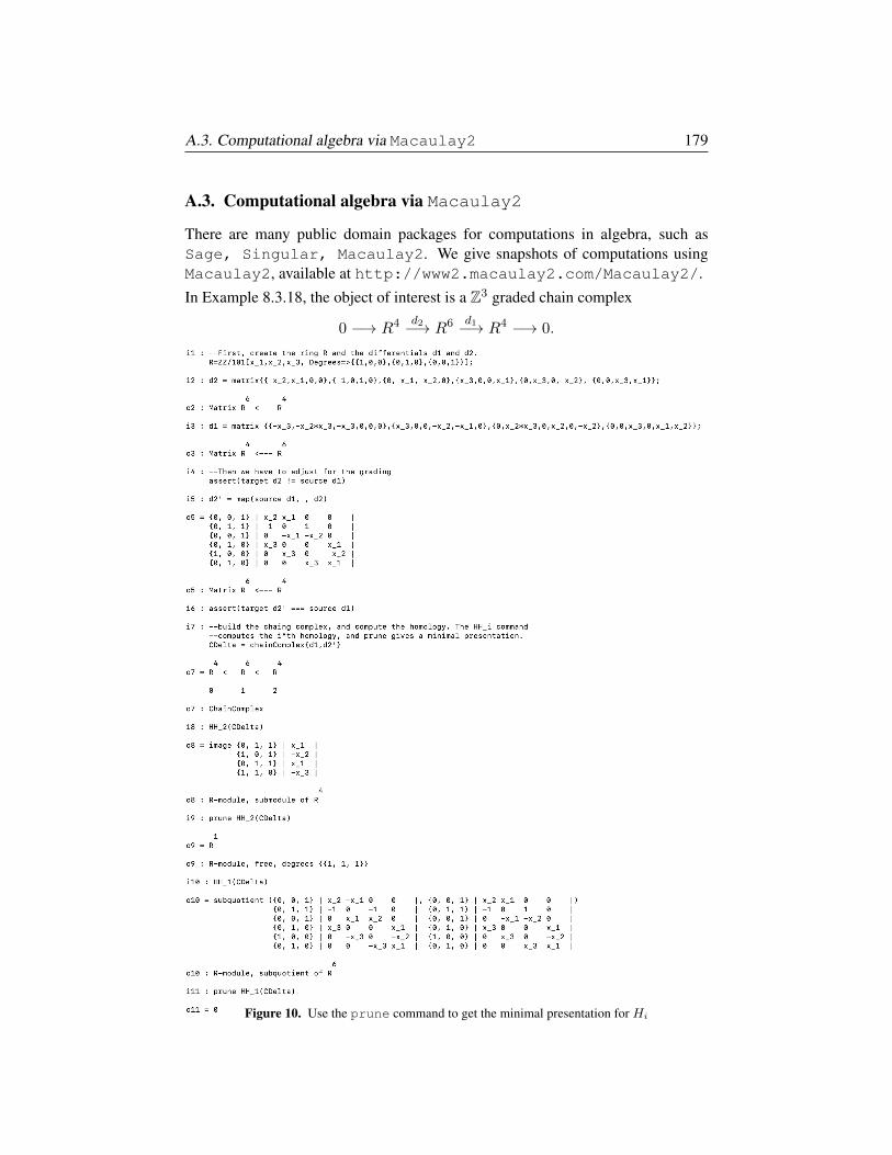
A.3. Computational algebra via Macaulay2 179
A.3. Computational algebra via Macaulay2
There are many public domain packages for computations in algebra, such asSage, Singular, Macaulay2. We give snapshots of computations usingMacaulay2, available at http://www2.macaulay2.com/Macaulay2/.
In Example 8.3.18, the object of interest is a Z3 graded chain complex
0 −→ R4 d2−→ R6 d1−→ R4 −→ 0.
Figure 10. Use the prune command to get the minimal presentation for Hi
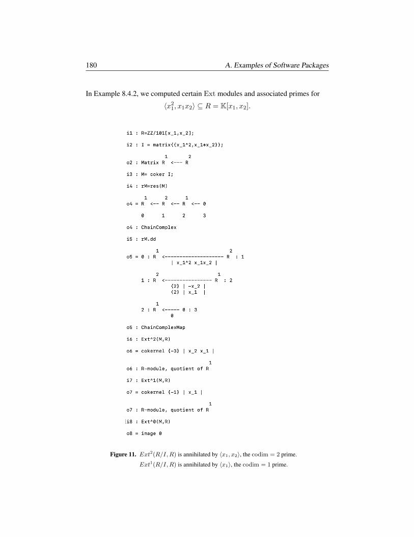
180 A. Examples of Software Packages
In Example 8.4.2, we computed certain Ext modules and associated primes for
〈x21, x1x2〉 ⊆ R = K[x1, x2].
Figure 11. Ext2(R/I,R) is annihilated by 〈x1, x2〉, the codim = 2 prime.
Ext1(R/I,R) is annihilated by 〈x1〉, the codim = 1 prime.
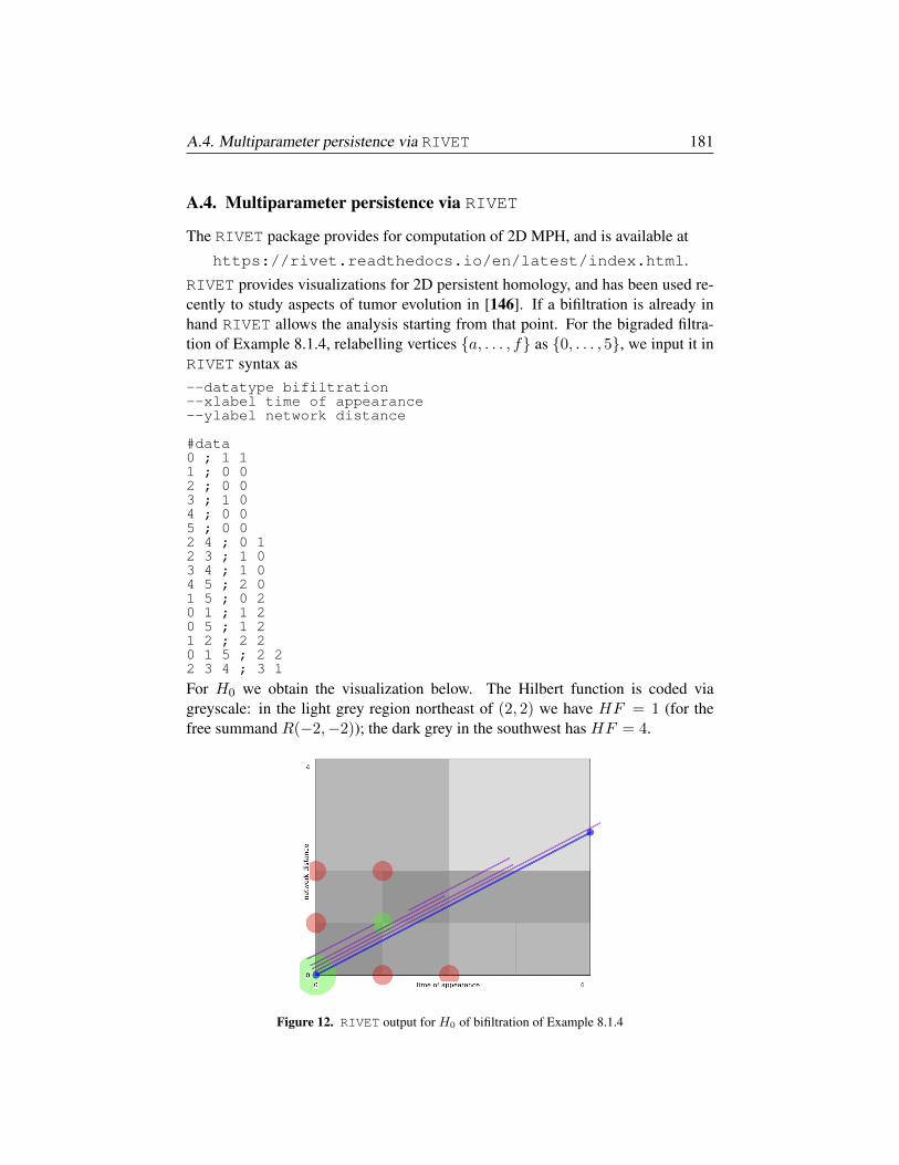
A.4. Multiparameter persistence via RIVET 181
A.4. Multiparameter persistence via RIVET
The RIVET package provides for computation of 2D MPH, and is available at
https://rivet.readthedocs.io/en/latest/index.html.
RIVET provides visualizations for 2D persistent homology, and has been used re-cently to study aspects of tumor evolution in [146]. If a bifiltration is already inhand RIVET allows the analysis starting from that point. For the bigraded filtra-tion of Example 8.1.4, relabelling vertices a, . . . , f as 0, . . . , 5, we input it inRIVET syntax as--datatype bifiltration--xlabel time of appearance--ylabel network distance
#data0 ; 1 11 ; 0 02 ; 0 03 ; 1 04 ; 0 05 ; 0 02 4 ; 0 12 3 ; 1 03 4 ; 1 04 5 ; 2 01 5 ; 0 20 1 ; 1 20 5 ; 1 21 2 ; 2 20 1 5 ; 2 22 3 4 ; 3 1
For H0 we obtain the visualization below. The Hilbert function is coded viagreyscale: in the light grey region northeast of (2, 2) we have HF = 1 (for thefree summand R(−2,−2)); the dark grey in the southwest has HF = 4.
Figure 12. RIVET output for H0 of bifiltration of Example 8.1.4
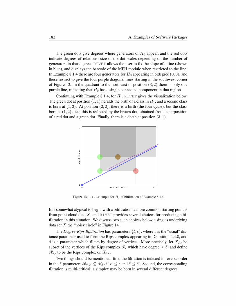
182 A. Examples of Software Packages
The green dots give degrees where generators of H0 appear, and the red dotsindicate degrees of relations; size of the dot scales depending on the number ofgenerators in that degree. RIVET allows the user to fix the slope of a line (shownin blue), and displays the barcode of the MPH module when restricted to the line.In Example 8.1.4 there are four generators for H0 appearing in bidegree (0, 0), andthese restrict to give the four purple diagonal lines starting in the southwest cornerof Figure 12. In the quadrant to the northeast of position (3, 2) there is only onepurple line, reflecting that H0 has a single connected component in that region.
Continuing with Example 8.1.4, for H1, RIVET gives the visualization below.The green dot at position (1, 1) heralds the birth of a class inH1, and a second classis born at (1, 2). At position (2, 2), there is a birth (the four cycle), but the classborn at (1, 2) dies; this is reflected by the brown dot, obtained from superpositionof a red dot and a green dot. Finally, there is a death at position (3, 1).
Figure 13. RIVET output for H1 of bifiltration of Example 8.1.4
It is somewhat atypical to begin with a bifiltration; a more common starting point isfrom point cloud data X , and RIVET provides several choices for producing a bi-filtration in this situation. We discuss two such choices below, using as underlyingdata set X the “noisy circle” in Figure 14.
The Degree-Rips Bifiltration has parameters δ, ε, where ε is the “usual” dis-tance parameter used to form the Rips complex appearing in Definition 4.4.8, andδ is a parameter which filters by degree of vertices. More precisely, let Xδ,ε besubset of the vertices of the Rips complex Rε which have degree ≥ δ, and defineRδ,ε to be the Rips complex on Xδ,ε.
Two things should be mentioned: first, the filtration is indexed in reverse orderin the δ parameter: Rδ′,ε′ ⊆ Rδ,ε if ε′ ≤ ε and δ ≤ δ′. Second, the correspondingfiltration is multi-critical: a simplex may be born in several different degrees.
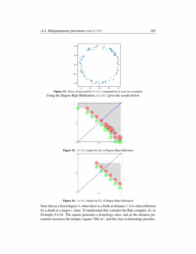
A.4. Multiparameter persistence via RIVET 183
Figure 14. Noisy circle used for RIVET computations in next two examplesUsing the Degree-Rips Bifiltration, RIVET gives the results below
Figure 15. RIVET output for H0 of Degree-Rips bifiltration
Figure 16. RIVET output for H1 of Degree-Rips bifiltration
Note that at a fixed degree δ, when there is a birth at distance ε′ it is often followedby a death at a larger ε value. To understand this consider the Rips complex R1 inExample 4.4.10. The square generates a homology class, and as the distance pa-rameter increases the (empty) square “fills in”, and the class in homology perishes.
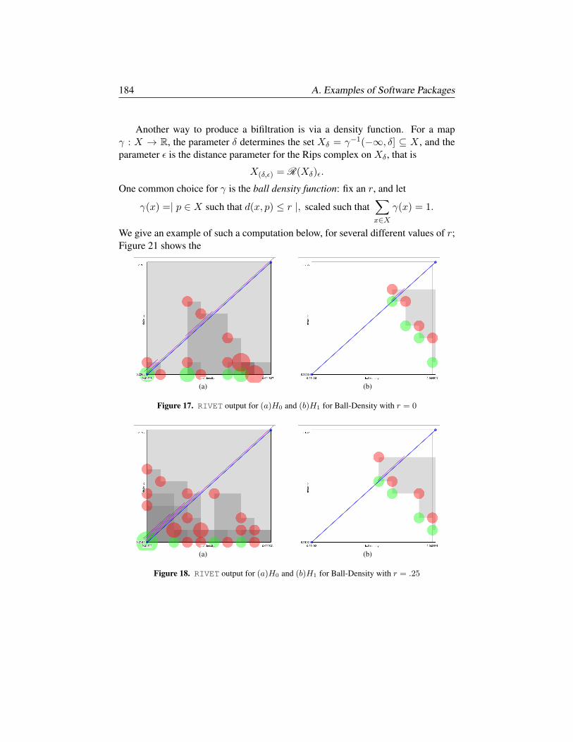
184 A. Examples of Software Packages
Another way to produce a bifiltration is via a density function. For a mapγ : X → R, the parameter δ determines the set Xδ = γ−1(−∞, δ] ⊆ X , and theparameter ε is the distance parameter for the Rips complex on Xδ, that is
X(δ,ε) = R(Xδ)ε.
One common choice for γ is the ball density function: fix an r, and let
γ(x) =| p ∈ X such that d(x, p) ≤ r |, scaled such that∑x∈X
γ(x) = 1.
We give an example of such a computation below, for several different values of r;Figure 21 shows the
(a) (b)
Figure 17. RIVET output for (a)H0 and (b)H1 for Ball-Density with r = 0
(a) (b)
Figure 18. RIVET output for (a)H0 and (b)H1 for Ball-Density with r = .25
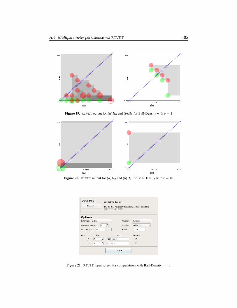
A.4. Multiparameter persistence via RIVET 185
(a) (b)
Figure 19. RIVET output for (a)H0 and (b)H1 for Ball-Density with r = 1
(a) (b)
Figure 20. RIVET output for (a)H0 and (b)H1 for Ball-Density with r = 10
Figure 21. RIVET input screen for computations with Ball-Density r = 1


Bibliography
[1] H. Adams, G. Carlsson, Evasion paths in mobile sensor networks, International Journal ofRobotics Research, 34, 90-104 (2014).
[2] P. Aluffi, Algebra: Chapter 0, Graduate Studies in Mathematics, 104. American MathematicalSociety, Providence, 2009.
[3] M. Artin, Algebra, Prentice Hall, Inc., Englewood Cliffs, NJ, 1991.
[4] M. Atiyah, I. G. MacDonald, Introduction to Commutative Algebra, Addison-Wesley, Read-ing, MA, 1969.
[5] D. Attali, H. Edelsbrunner, Y. Mileyko, Weak witnesses for Delaunay triangulations of sub-manifolds, Proc. 2007 ACM symposium on solid and physical modeling, 143-150, (2007).
[6] U. Bauer, H. Edelsbrunner, The Morse theory of Cech and Delaunay complexes, Trans. Amer.Math. Soc., 369, 3741-3762 (2017).
[7] U. Bauer, M. Lesnick, Induced matchings and the algebraic stability of persistence barcodes,J. Comput. Geom. 6, 162-191 (2015).
[8] U. Bauer, M. Lesnick, Persistence Diagrams as Diagrams: A Categorification of the StabilityTheorem, Topological Data Analysis: the Abel Symposium 2018, Springer, 67-96 (2020).
[9] P. Bendich, H. Edelsbrunner, D. Morozov, A. Patel, Homology and robustness of level andinterlevel sets, Homology Homotopy Appl., 15, 51-72 (2013).
[10] P. Bendich, J.S. Marron, E. Miller, A. Pieloch, S. Skwerer, Persistent homology analysis ofbrain artery trees, Ann. Appl. Stat., 10, 198-218 (2016).
[11] S. Biasotti, A. Cerri, P. Frosini, D. Giorgi, C. Landi, Multidimensional size functions for shapecomparison, Journal of Mathematical Imaging and Vision 32, 161-179 (2008).
[12] H. Bjerkevik, On the Stability of Interval Decomposable Persistence Modules, Discrete andComputational Geometry, 66, 92-121 (2021).
[13] H. Bjerkevik, M. Botnan, Computational complexity of the interleaving distance, 34th Inter-national Symposium on Computational Geometry, Leibniz Int. Proc. Inform., 99, (2018).
[14] H. Bjerkevik, M. Botnan, M. Kerber, Computing the Interleaving Distance is NP-hard, Foun-dations of Computational Mathematics, 20, 1237-1271 (2020).
[15] H. Bjerkevik, M. Lesnick, `p-Distances on Multiparameter Persistence Modules, preprint,arXiv:2106.13589, (2021).
187
188 Bibliography
[16] A. Bjorner, Nerves, fibers and homotopy groups, J. Combin. Theory Ser. A, 102, 88-93 (2003).
[17] A. Bjorner, M. Tanzer, Combinatorial Alexander duality—a short and elementary proof, Dis-crete Comput. Geom., 42, 586-593 (2009).
[18] M. Botnan, M. Lesnick, Algebraic stability of zigzag persistence modules, Algebr. Geom.Topol., 18, 3133-3204 (2018).
[19] M. Botnan, M. Lesnick, An Introduction to Multiparameter Persistence, preprint, 2021.
[20] R. Bott, Morse theory indomitable, Inst. Hautes Etudes Sci. Publ. Math, 68, 99-114, (1989).
[21] R. Bott, L. Tu, Differential forms in algebraic topology, Springer-Verlag, New York-Berlin(1982)
[22] P. Bubenik, V. de Silva, J. Scott, Metrics for generalized persistence modules, Foundations ofComp. Math., 15, 1501-1531 (2015).
[23] P. Bubenik, J. Scott, Categorification of persistent homology, Discrete and ComputationalGeometry 51, 600-627 (2014).
[24] H. Byrne, H. Harrington, R. Muschel, G. Reinert, B. Stolz, U. Tillmann, Topology charac-terises tumour vasculature, Math. Today (Southend-on-Sea), 55, 206-210 (2019).
[25] G. Carlsson, Topology and data, Bulletin of the American Mathematical Society, 46, 255-308(2009).
[26] G. Carlsson, V. de Silva, ZigZag Persistence, Found. Comput. Math., 10, 367-405 (2010).
[27] G. Carlsson, V. de Silva, S. Kalisnik, D. Morozov, Parametrized homology via zigzag persis-tence, Algebr. Geom. Topol., 19, 657-700 (2019).
[28] G. Carlsson, A. Levine, M. Nicolau, Topology based data analysis identifies a subgroup ofbreast cancers with a unique mutational profile and excellent survival, PNAS, 108 (2011),7265-7270.
[29] G. Carlsson, G. Singh, A. Zomorodian, Computing multidimensional persistence, Journal ofComputational Geometry, 1, 72-100 (2010).
[30] G. Carlsson, M. Vejdemo-Johansson, Topological Data Analysis with Applications, Cam-bridge University Press, to appear.
[31] G. Carlsson, J. Skryzalin, Numeric invariants from multidimensional persistence, J. Appl.Comput. Topol., 1, 89-119 (2017).
[32] G. Carlsson, A. Zomorodian, Computing persistent homology, Discrete Comput. Geom., 33,249-274 (2005).
[33] G. Carlsson, A. Zomorodian, The theory of multidimensional persistence, Discrete & Com-putational Geometry, 42, 71-93 (2009).
[34] M. Carriere, A. Blumberg, Multiparameter Persistence Images for Topological MachineLearning, Advances in Neural Information Processing Systems 33 (NeurIPS 2020), 13 pp,(2020).
[35] W. Chacholski, O. Gafvert, Stable Invariants for Multidimensional Persistence, in preparation.
[36] W. Chacholski, M. Scolamiero, and F. Vaccarino, Combinatorial presentation of multidimen-sional persistent homology, Journal of Pure and Applied Algebra, 221, 1055-1075 (2017).
[37] J. Chan, G. Carlsson, R. Rabadan, Topology of viral evolution, PNAS, 110, 18566-18571(2013).
[38] R. Charney, M. Davis, The Euler Chracteristic of a nonpositively curved, piecewise Euclideanmanifold, Pacific J. Math. 171, 117-137 (1995).
[39] F. Chazal, D. Cohen-Steiner, M. Glisse, L. Guibas, S. Oudot, Proximity of persistence modulesand their diagrams, Proceedings of the 25th Annual Symposium on Computational Geometry,SCG ’09, 237-246 (2009).
Bibliography 189
[40] F. Chazal, V. de Silva, M. Glisse, S. Oudot, The structure and stability of persistence modules,SpringerBriefs in Mathematics, Springer, (2016).
[41] F. Chazal, A. Lieutier, Weak feature size and persistant homology: computing homology ofsolids in Rn from noisy data samples, Computational geometry (SCG’05), ACM, New York,255-262 (2005).
[42] F. Chazal, A. Lieutier, Topology guaranteeing manifold reconstruction using distance functionto noisy data, Computational geometry (SCG’06), ACM, New York, 112-118 (2006).
[43] F. Chazal, S. Oudot, Towards persistence-based reconstruction in Euclidean spaces, Compu-tational geometry (SCG’08), ACM, New York, 232-241 (2008).
[44] D. Cohen-Steiner, H. Edelsbrunner, J. Harer, Stability of persistence diagrams, Discrete Com-put. Geom. 37, 103-120 (2007).
[45] D. Cohen-Steiner, H. Edelsbrunner, J. Harer, Extending persistence using Poincare and Lef-schetz duality, Found. Comput. Math., 9, 79-103 (2009).
[46] D. Cohen-Steiner, H. Edelsbrunner, D. Morozov, Vines and Vineyards by Updating Persis-tence in Linear Time, Proceedings of the Annual ACM Symposium on Computational Geom-etry, 119-126 (2006).
[47] D. Cox, J. Little, D. O’Shea, Ideals, Varieties and Algorithms, third edition, UndergraduateTexts in Math., Springer, New York, 2007.
[48] D. Cox, J. Little, H. Schenck, Toric Varieties, AMS Graduate Studies in Math, AMS, (2010).[49] M. Davis, B. Okun, Vanishing theorems and conjectures for the l2- homology of right-angled
Coxeter groups, Geom. Topo., 5, 7-74 (2001).[50] M. DeGroot, Reaching a consensus, Journal of the American Statistical Association, 69, 118-
121 (1974).[51] V. de Silva, G. Carlsson, Topological estimation using witness complexes, Proc. 1st Euro-
graphics conference on Point-Based Graphics, 157-166 (2004).[52] V. de Silva, R. Ghrist, Coordinate-free Coverage in Sensor Networks with Controlled Bound-
aries via Homology, International Journal of Robotics Research, 25, 1205-1222 (2006).[53] V. de Silva, R. Ghrist, Coverage in sensor networks via persistent homology, Algebr. Geom.
Topol. 7, 339-358 (2007).[54] V. de Silva, R. Ghrist, Homological Sensor Networks, Notices of the A.M.S., 54, 10-17 (2007).[55] V. de Silva, D. Morozov, M. Vejdemo-Johansson, Dualities in Persistent Homology, Inverse
Problems, 27, 17pp, (2011).[56] V. de Silva, E. Munch, A. Patel, Categorified Reeb graphs, Discrete Comput. Geom.,55, 854-
906 (2016).[57] V. de Silva, E. Munch, A. Stefanou, Theory of interleavings on categories with a flow, Theory
Appl. Categ. 33, 583-607 (2018).[58] T. Dey, F. Fan, Y. Wang, Computing topological persistence for simplicial maps, Computa-
tional geometry (SoCG’14), ACM, New York, 345-354 (2014).[59] T. Dey, T. Li, Y. Wang, An efficient algorithm for 1-dimensional persistent path homology,
36th International Symposium on Computational Geometry, Leibniz Int. Proc. Inform, 136,15pp (2019).
[60] T. Dey, Y. Wang, Computational Topology for Data Analysis, Cambridge University Press, toappear.
[61] B. Di Fabio, C. Landi, Reeb graphs of piecewise linear functions, Graph-based representa-tions in pattern recognition Lecture Notes in Comput. Sci., 10310, 23-35 (2017).
[62] B. Di Fabio, C. Landi, The edit distance for Reeb graphs of surfaces, Discrete Comput. Geom.,55, 423-461 (2016).
190 Bibliography
[63] B. Di Fabio, C. Landi, Reeb graphs of curves are stable under function perturbations, Math.Methods Appl. Sci., 35, 1456-1471 (2012).
[64] H. Edelsbrunner, D. Kirkpatrick, R. Seidel, On the shape of a set of points in the plane, IEEETrans. Info. Theory, 29, 551-559 (1983).
[65] H. Edelsbrunner, D. Letscher, A. Zomorodian, Topological persistence and simplification,Discrete Comput. Geom., 28, 511-533 (2002).
[66] H. Edelsbrunner, J. Harer, Persistent homology — A survey, Contemporary Mathematics, 453,257-282 (2008).
[67] H. Edelsbrunner, J. Harer, Computational Topology: An Introduction, American MathematicalSociety, Providence (2010).
[68] H. Edelsbrunner, M. Kerber, Alexander duality for functions: the persistent behavior of landand water and shore, Computational geometry (SCG’12), 249-258, (2012).
[69] H. Edelsbrunner, D. Morozov, Persistent homology: theory and practice, European Congressof Mathematics, Eur. Math. Soc., Zurich, 31-50 (2013).
[70] D. Eisenbud, Commutative Algebra with a View Toward Algebraic Geometry, Graduate Textsin Math. 150, Springer, New York, 2000.
[71] D. Eisenbud, C. Huneke, W. Vasconcelos, Direct methods for primary decomposition, Invent.Math., 110, 207-235 (1992).
[72] N. Friedkin, E. Johnsen, Social influence and opinions, J. Mathematical Sociology, 15, 193-206 (1990).
[73] P. Frosini, A distance for similarity classes of submanifolds of a Euclidean space, Bulletin ofthe Australian Mathematical Society, 42, 407-415 (1990).
[74] P. Frosini, Discrete computation of size functions. J. Combin. Inform. System Sci., 17, 132-250(1992).
[75] P. Frosini, C. Landi, Size functions and morphological transformations, Acta Appl. Math. 49,85-104 (1997).
[76] W. Fulton, Algebraic Topology-A first course, Graduate Texts in Math. 153, Springer, NewYork, 1995.
[77] P. Gabriel, Unzerlegbare darstellung I, Manuscripta Math., 6, 71-103 (1972).
[78] R. Ghrist, Barcodes: the persistent topology of data, Bull. Amer. Math. Soc., 45, 61-75 (2008).
[79] R. Ghrist, Elementary Applied Topology, ed. 1.0, Createspace, (2014).
[80] R. Ghrist, Homological algebra and data, The mathematics of data, p. 273-325, IAS/Park CityMath. Ser., 25, Amer. Math. Soc., Providence, 2018.
[81] R. Ghrist, Y. Hiraoka, Applications of sheaf cohomology and exact sequences to networkcoding, Proc. NOLTA, 2011.
[82] R. Ghrist, S. Krishnan, Positive Alexander duality for pursuit and evasion, SIAM J. Appl.Algebra Geom., 1, 308-327 (2017).
[83] M. Greenberg, J. Harper, Algebraic Topology: A First Course, Benjamin/Cummings, Reading,MA, 1981. Reprinted by Westview Press, Boulder, CO.
[84] P. Griffiths, J. Harris, Principles of algebraic geometry, Pure and Applied Mathematics. JohnWiley & Sons, New York, 1978.
[85] L. Guibas, S. Oudot, Reconstruction using witness complexes, Discrete and ComputationalGeometry, 40, 325-356 (2008).
[86] J. Hansen, R. Ghrist, Toward a spectral theory of cellular sheaves, J. Appl. Comput. Topol., 3,315-358 (2019).

Bibliography 191
[87] J. Hansen, R. Ghrist, Opinion dynamics on discourse sheaves, SIAM J. Appl. Math.,81, 2033-2060 (2021).
[88] H. Harrington, N. Otter, H. Schenck, U. Tillmann, Stratifying multiparameter persistent ho-mology, SIAM J. Appl. Algebra Geom., 3, 439-471 (2019).
[89] J. Harris, Algebraic Geometry: A First Course, Graduate Texts in Math. 133, Springer, NewYork, 1992.
[90] R. Hartshorne, Algebraic Geometry, Graduate Texts in Math. 52, Springer, New York, 1977.
[91] A. Hatcher, Algebraic Topology, Cambridge Univ. Press, Cambridge, 2002.
[92] Y. H. He, The Calabi-Yau landscape: from geometry to physics to machine learning, Springer,New York, 2021.
[93] T. Hungerford, Algebra, Graduate Texts in Math. 73, Springer, New York, 2002.
[94] X. Jiang, L.-H. Lim, Y. Yao, Y. Ye, Statistical ranking and combinatorial Hodge theory, Math.Program., 127, 203-244 (2011).
[95] S. Kalisnik, Alexander duality for parametrized homology, Homology Homotopy Appl., 15,227-243 (2013).
[96] S. Kalisnik, Tropical coordinates on the space of persistence barcodes, Found. Comput. Math.,19, 101-129 (2019).
[97] S. Kalisnik, C. Lehn, V. Limic, Geometric and probabilistic limit theorems in topological dataanalysis, Adv. in Appl. Math., 131, 36pp, (2021).
[98] L. Kanari, A. Garin, K. Hess, From trees to barcodes and back again: theoretical and statisticalperspectives, Algorithms (Basel), 13, 27pp (2020).
[99] M. Kerber, M. Lesnick, S. Oudot, Exact computation of the matching distance on 2-parameterpersistence modules, J. Comput. Geom., 11, 4-25 (2020).
[100] K. Knudson, A refinement of multidimensional persistence, Homology, Homotopy and Appli-cations, 10, 259-281 (2008).
[101] D. Kozlov, Combinatorial algebraic topology, Algorithms and Computation in Mathematics,21. Springer, Berlin (2008).
[102] S. Lang, Algebra, Graduate Texts in Math, 211 Springer, New York, 2002.
[103] M. Lesnick, The theory of the interleaving distance on multidimensional persistence modules,Found. Comput. Math., 15 613-650 (2015).
[104] R. Lewis, Spectral Sequences and Applied Topology, Ph.D. thesis, Stanford (2016).
[105] R. Lewis, D. Morozov, Parallel computation of persistent homology using the blowup complexAnnual ACM Symposium on Parallelism in Algorithms and Architectures, 323-331, (2015).
[106] L. H. Lim, Hodge Laplacians on Graphs, SIAM Rev., 62, 685-715, (2020).
[107] S. MacLane, Categories for the working mathematician, Graduate Texts in Mathematics, Vol.5. Springer-Verlag, New York-Berlin, 1971.
[108] Y. Matsumoto, An Introduction to Morse Theory, American Mathematical Society, Provi-dence, RI, 2002.
[109] J. McCleary, A User’s Guide to Spectral Sequences, Cambridge Univ. Press, Cambridge, 2001.
[110] E. Miller, Fruit flies and moduli: interactions between biology and mathematics, Notices Amer.Math. Soc., 62, 1178-1184 (2015).
[111] J. Milnor, Morse Theory, Princeton University Press, 1963
[112] N. Milosavljevic, D. Morozov, P. Skraba, Zigzag persistent homology in matrix multiplicationtime, Computational geometry (SCG’11), 216-225, (2011).
192 Bibliography
[113] D. Morozov, Persistence algorithm takes cubic time in worst case, Proceedings of Topology-Based Methods in Visualization, (2013).
[114] D. Morozov, K. Beketayev, G. Weber, Interleaving Distance between Merge Trees, Proceed-ings of Topology-Based Methods in Visualization, (2013).
[115] M. Morse, Relations between the critical points of a real function of n independent variables,Trans. Amer. Math. Soc., 27, 345-396 (1925).
[116] M. Morse, The foundations of a theory in the calculus of variations in the large, Trans. Amer.Math. Soc. 30, 213-274 (1928).
[117] M. Morse, Rank and span in functional topology, Ann. of Math, 41, 419-454 (1940).
[118] E. Munch, B. Wang, Convergence between categorical representations of Reeb space and map-per, 32nd International Symposium on Computational Geometry, Leibniz Int. Proc. Inform.,34, 461-475 (2016).
[119] J. Munkres, Elements of Algebraic Topology, Addison-Wesley, Reading, MA, 1984. Reprintedby Westview Press, Boulder, CO.
[120] B. Nelson, Parameterized Topological Data Analysis, Ph.D. thesis, Stanford (2020).
[121] P. Niyogi, S. Smale, S. Weinberger, Finding the homology of submanifolds with high confi-dence from random samples, Discrete Comput. Geom., 39, 419-441 (2008).
[122] P. Oesterling, C. Heine, G. Weber, D. Morozov, G. Scheuermann, Computing and visualizingtime-varying merge trees for high-dimensional data, Topological methods in data analysis andvisualization, IV, Math. Vis., Springer, 87-101 (2017).
[123] N. Otter, M. Porter, U. Tillmann, P. Grindrod, H. Harrington, A roadmap for the computationof persistent homology, EJP Data Science, 6, 1-38 (2017).
[124] S. Oudot, Persistence theory: from quiver representations to data analysis, American Mathe-matical Society, Providence, RI, 2015.
[125] J. Perea, A brief history of persistence, Morfismos, 23, 1-16 (2019).
[126] L. Polterovich, D. Rosen, K. Samvelyan, J. Zhang, Topological Persistence in Geometry andAnalysis, AMS University Lecture Series, AMS, 2020.
[127] R. Rabadan, A. Blumberg, Topological Data Analysis for Genomics and Evolution: Topologyin Biology, Cambridge University Press, 2020.
[128] E. Riehl, Category Theory in Context, Dover, 2016.
[129] V. Robins, Towards computing homology from finite approximations, Topology Proceedings,24, 503-532 (1999).
[130] V. Robins, K. Turner, Principal component analysis of persistent homology rank functionswith case studies of spatial point patterns, sphere packing and colloids, Phys. D, 334, 99-117(2016).
[131] M. Robinson, Topological signal processing, Springer, Heidelberg, 2014.
[132] J. J. Rotman, Advanced Modern Algebra, Prentice-Hall, Upper Saddle River, NJ, 2002.
[133] H. Schenck, Computational Algebraic Geometry, Cambridge Univ. Press, Cambridge, 2003.
[134] M. Scolamiero, W. Chacholski, A. Lundman, R. Ramanujam, S. Oberg, MultidimensionalPersistence and Noise, Foundations of Computational Mathematics, 17, 1367-1406 (2017).
[135] I. Singer, J. Thorpe, Lecture notes on elementary topology and geometry, Undergraduate Textsin Math., Springer, New York, 1967.
[136] G. Singh, F. Memoli, T. Ishkhanov, G. Sapiro, G. Carlsson, D. Ringach, Topological analysisof population activity in visual cortex, Journal of Vision, 8, 1-18 (2008).
[137] E. Spanier, Algebraic Topology, McGraw-Hill, New York, 1966. Reprinted by Springer Ver-lag, New York.

Bibliography 193
[138] M. Spivak, Calculus on Manifolds, W.A. Benjamin, New York, 1965.
[139] J. Stewart, Calculus, Cengage, 2020.
[140] B. Stolz, H. Harrington, M. Porter, Persistent homology of time-dependent functional net-works constructed from coupled time series, Chaos 27, 17pp, (2017).
[141] B. Stolz, J. Tanner, H. Harrington, V. Nanda, Geometric anomaly detection in data, Proceed-ings of the National Academy of Sciences, 117, 19664-19669, (2021).
[142] M. Taylor, Towards a mathematical theory of influence and attitude change, Human Relations,21, 121-139 (1968).
[143] K. Turner, Medians of populations of persistence diagrams, Homology Homotopy Appl., 22,255-282 (2020).
[144] K. Turner, S. Mukherjee, D. Boyer, Persistent homology transform for modeling shapes andsurfaces, Information and Inference, 3, 310-344 (2014).
[145] K. Turner, Y. Mileyko, S. Mukherjee, J. Harer, Frechet means for distributions of persistencediagrams, Discrete Comput. Geom., 52, 44-70 (2014).
[146] O. Vipond, J. Bull, P. Macklin, U. Tillman, C. Pugh, H. Byrne, H. Harrington, Multiparameterpersistent homology landscapes identify immune cell spatial patterns in tumors, Proceedingsof the National Academy of Sciences, 118, 9pp, (2021).
[147] C. Voisin, Hodge theory and complex algebraic geometry I, II, Cambridge Studies in Ad-vanced Mathematics, 76. Cambridge University Press, Cambridge, 2007.
[148] C. Webb, Decomposition of graded modules, Proceedings of the American Mathematical So-ciety, 94, 565-571 (1985).
[149] C. Weibel, An introduction to homological algebra, Cambridge Univ. Press, Cambridge, 1994.
[150] S. Weinberger, What is. . . persistent homology?, Notices Amer. Math. Soc. 58, 36-39 (2011).
[151] M. Wright, X. Zheng, Topological data analysis on simple English Wikipedia articles, PUMPJ. Undergrad. Res., 3, 308-328 (2020).
[152] A. Zomorodian, Computing and Comprehending Topology: Persistence and HierarchicalMorse Complexes, Ph.D. thesis, University of Illinois at Urbana-Champaign, 2001.
[153] A. Zomorodian, Topology for computing, Cambridge University Press, Cambridge, 2005.