algebraic properties of cellular automata - digital …odlyzko/doc/arch/cellular.automata… ·...
TRANSCRIPT

LaTEX filename: Algebraic.tex (Paper: 1.2 [2]) 12:08 p.m. October 20, 1993
Algebraic Propertiesof Cellular Automata
1 9 8 4
Cellular automata are discrete dynamical systems,of simple construction but complexand varied behaviour. Algebraic techniques are used to give an extensive analysis ofthe global properties of a class of finite cellular automata. The complete structureof state transition diagrams is derived in terms of algebraic and number theoreticalquantities. The systems are usually irreversible, and are found to evolve throughtransients to attractors consisting of cycles sometimes containing a large number ofconfigurations.
1. Intr oduction
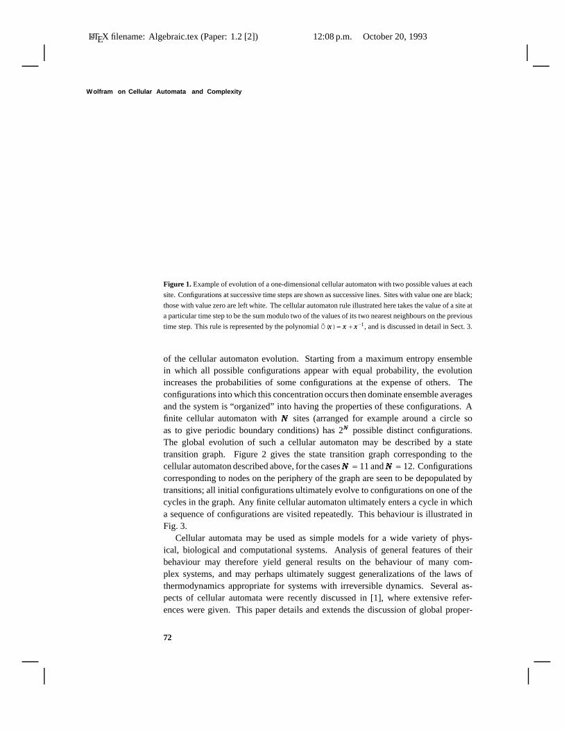
In the simplest case, a cellular automaton consists of a line of sites with each sitecarrying a value 0 or 1. The site values evolve synchronously in discrete timesteps according to the values of their nearest neighbours. For example, the rule forevolution could take the value of a site at a particular time step to be the sum modulotwo of the values of its two nearest neighbours on the previous time step. Figure 1shows the pattern of nonzero sites generated by evolution with this rule from an initialstate containing a single nonzero site. The pattern is found to be self-similar, and ischaracterized by a fractal dimension log2 3. Even with an initial state consisting of arandom sequence of 0 and 1 sites (say each with probability 1
2 ), the evolution of sucha cellular automaton leads to correlations between separated sites and the appearanceof structure. This behaviour contradicts the second law of thermodynamics forsystems with reversible dynamics, and is made possible by the irreversible nature
Coauthored with Olivier Martin and Andrew M. Odlyzko. Originally published in Communications in MathematicalPhysics, volume 93, pages 219–258 (March 1984).
71
LaTEX filename: Algebraic.tex (Paper: 1.2 [2]) 12:08 p.m. October 20, 1993
Wolfram on Cellular Automata and Complexity
Figure 1. Example of evolution of a one-dimensional cellular automaton with two possible values at each
site. Configurations at successive time steps are shown as successive lines. Sites with value one are black;
those with value zero are left white. The cellular automaton rule illustrated here takes the value of a site at
a particular time step to be the sum modulo two of the values of its two nearest neighbours on the previous
time step. This rule is represented by the polynomial Ö(x� ) = x� + x� - 1, and is discussed in detail in Sect. 3.
of the cellular automaton evolution. Starting from a maximum entropy ensemblein which all possible configurations appear with equal probability, the evolutionincreases the probabilities of some configurations at the expense of others. Theconfigurations into which this concentration occurs then dominate ensemble averagesand the system is “organized” into having the properties of these configurations. Afinite cellular automaton with N
�sites (arranged for example around a circle so
as to give periodic boundary conditions) has 2N�
possible distinct configurations.The global evolution of such a cellular automaton may be described by a statetransition graph. Figure 2 gives the state transition graph corresponding to thecellular automaton described above, for the cases N
�= 11 and N
�= 12. Configurations
corresponding to nodes on the periphery of the graph are seen to be depopulated bytransitions; all initial configurations ultimately evolve to configurations on one of thecycles in the graph. Any finite cellular automaton ultimately enters a cycle in whicha sequence of configurations are visited repeatedly. This behaviour is illustrated inFig. 3.
Cellular automata may be used as simple models for a wide variety of phys-ical, biological and computational systems. Analysis of general features of theirbehaviour may therefore yield general results on the behaviour of many com-plex systems, and may perhaps ultimately suggest generalizations of the laws ofthermodynamics appropriate for systems with irreversible dynamics. Several as-pects of cellular automata were recently discussed in [1], where extensive refer-ences were given. This paper details and extends the discussion of global proper-
72

LaTEX filename: Algebraic.tex (Paper: 1.2 [2]) 12:08 p.m. October 20, 1993
Algebraic Propertiesof CellularAutomata(1984)
Figure 2. Global state transition diagrams for finite cellular automata with size N and periodic boundary
conditions evolving according to the rule Ö(x� ) = x� + x� - 1 , as used in Fig. 1, and discussed extensively
in Sect. 3. Each node in the graphs represents one of the 2N�
possible configurations of the N sites.
The directed edges of the graphs indicate transitions between these configurations associated with single
time steps of cellular automaton evolution. Each cycle in the graph represents an “attractor” for the
configurations corresponding to the nodes in trees rooted on it.
ties of cellular automata given in [1]. These global properties may be describedin terms of properties of the state transition graphs corresponding to the cellularautomata.
This paper concentrates on a class of cellular automata which exhibit the simpli-fying feature of “additivity”. The configurations of such cellular automata satisfyan “additive superposition” principle, which allows a natural representation of theconfigurations by characteristic polynomials. The time evolution of the configura-tions is represented by iterated multiplication of their characteristic polynomials byfixed polynomials. Global properties of cellular automata are then determined byalgebraic properties of these polynomials, by methods analogous to those used inthe analysis of linear feedback shift registers [2, 3]. Despite their amenability toalgebraic analysis, additive cellular automata exhibit many of the complex featuresof general cellular automata.
73

LaTEX filename: Algebraic.tex (Paper: 1.2 [2]) 12:08 p.m. October 20, 1993
Wolfram on Cellular Automata and Complexity
N = 12 N = 63 N = 71 N = 192
Figure 3. Evolution of cellular automata with N sites arranged in a circle (periodic boundary conditions)
according to the rule Ö(x� ) = x� + x� - 1 (as used in Fig. 1 and discussed in Sect. 3). Finite cellular automata
such as these ultimately enter cycles in which a sequence of configurations are visited repeatedly. This
behaviour is evident here for N = 12, 63, and 192. For N = 71, the cycle has length 235 - 1.
Having introduced notation in Sect. 2, Sect. 3 develops algebraic techniques forthe analysis of cellular automata in the context of the simple cellular automatonillustrated in Fig. 1. Some necessary mathematical results are reviewed in theappendices. Section 4 then derives general results for all additive cellular automata.The results allow more than two possible values per site, but are most completewhen the number of possible values is prime. They also allow influence on theevolution of a site from sites more distant than its nearest neighbours. The resultsare extended in Sect. 4D to allow cellular automata in which the sites are arranged
74

LaTEX filename: Algebraic.tex (Paper: 1.2 [2]) 12:08 p.m. October 20, 1993
Algebraic Propertiesof CellularAutomata(1984)
in a square or cubic lattice in two, three or more dimensions, rather than just on aline. Section 4E then discusses generalizations in which the cellular automaton timeevolution rule involves several preceding time steps. Section 4F considers alternativeboundary conditions. In all cases, a characterization of the global structure of thestate transition diagram is found in terms of algebraic properties of the polynomialsrepresenting the cellular automaton time evolution rule.
Section 5 discusses non-additive cellular automata, for which the algebraic tech-niques of Sects. 3 and 4 are inapplicable. Combinatorial methods are neverthelessused to derive some results for a particular example.
Section 6 gives a discussion of the results obtained, comparing them with thosefor other systems.
2. Formalism
We consider first the formulation for one-dimensional cellular automata in whichthe evolution of a particular site depends on its own value and those of its nearestneighbours. Section 4 generalizes the formalism to several dimensions and moreneighbours.
We take the cellular automaton to consist of N�
sites arranged around a circle (soas to give periodic boundary conditions). The values of the sites at time step t� aredenoted a� (t� )
0 ������ a� (t� )N�
- 1. The possible site values are taken to be elements of a finitecommutative ring Ùk
� with k
elements. Much of the discussion below concerns thecase Ùk
� = Úk� , in which site values are conveniently represented as integers modulo k
.
In the example considered in Sect. 3, Ùk� = Ú2, and each site takes on a value 0 or 1.
The complete configuration of a cellular automaton is specified by the values of itsN�
sites, and may be represented by a characteristic polynomial (generating function)(cf. [2, 3])
(2.1)A (t�)(x� ) =
N�
- 1
i=0
a� (t� )i x� i �
where the value of site i�
is the coefficient of x� i , and all coefficients are elements of thering Ùk
� . We shall often refer to configurations by their corresponding characteristicpolynomials.
It is often convenient to consider generalized polynomials containing both positiveand negative powers of x� : such objects will be termed “dipolynomials”. In general,H (x� ) is a dipolynomial if there exists some integer m� such that x� m� H (x� ) is an ordinarypolynomial in x� . As discussed in Appendix A, dipolynomials possess divisibilityand congruence properties analogous to those of ordinary polynomials.
Multiplication of a characteristic polynomial A(x� ) by x� –j�
yields a dipolynomialwhich represents a configuration in which the value of each site has been transferred(shifted) to a site j
�places to its right (left). Periodic boundary conditions in the
75
LaTEX filename: Algebraic.tex (Paper: 1.2 [2]) 12:08 p.m. October 20, 1993
Wolfram on Cellular Automata and Complexity
cellular automaton are implemented by reducing the characteristic dipolynomialmodulo the fixed polynomial x� N
�- 1 at all stages, according to
(2.2)i
a� ix� i mod (x� N
�- 1) =
N�
- 1
i=0
�j� a� i+j
�N� �x� i �
Note that any dipolynomial is congruent modulo (x� N�
- 1) to a unique ordinarypolynomial of degree less than N
�.
In general, the value a� (t� )i of a site in a cellular automaton is taken to be an arbitrary
function of the values a� (t� - 1)i- 1 , a� (t� - 1)
i , and a� (t� - 1)i+1 at the previous time step. Until Sect. 5,
we shall consider a special class of “additive” cellular automata which evolve withtime according to simple linear combination rules of the form (taking the site indexi�
modulo N�
)
(2.3)a� (t� )i = a- 1a� (t� - 1)
i- 1 + a0 a� (t� - 1)i + a+1a� (t� - 1)
i+1 �where the aj
� are fixed elements of Ùk� , and all arithmetic is performed in Ùk
� . Thistime evolution may be represented by multiplication of the characteristic polynomialby a fixed dipolynomial in x� ,
(2.4)Ö(x� ) = a - 1x� + a0 + a+1x� - 1 �according to
(2.5)A (t� )(x� ) ” Ö(x� )A (t� - 1)(x� ) mod (x� N�
- 1) �where arithmetic is again performed in Ùk
� . Additive cellular automata obey anadditive superposition principle which implies that the configuration obtained byevolution for t� time steps from an initial configuration A (0)(x� ) + B (0)(x� ) is identicalto A (t
�)(x� ) + B (t
�)(x� ), where A (t
�)(x� ) and B (t
�)(x� ) are the results of separate evolution of
A (0)(x� ) and B (0)(x� ), and all addition is performed in Ùk� . Since any initial configuration
can be represented as a sum of “basis” configurations Á(x� ) = x� j�
containing singlenonzero sites with unit values, the additive superposition principle determines theevolution of all configurations in terms of the evolution of Á(x� ). By virtue of thecyclic symmetry between the sites it suffices to consider the case j
�= 0.
3. A Simple Example
A. Intr oduction
This section introduces algebraic techniques for the analysis of additive cellularautomata in the context of a specific simple example. Section 4 applies the techniquesto more general cases. The mathematical background is outlined in the appendices.
76

LaTEX filename: Algebraic.tex (Paper: 1.2 [2]) 12:08 p.m. October 20, 1993
Algebraic Propertiesof CellularAutomata(1984)
The cellular automaton considered in this section consists of N�
sites arrangedaround a circle, where each site has value 0 or 1. The sites evolve so that at eachtime step the value of a site is the sum modulo two of the values of its two nearestneighbours at the previous time step:
(3.1)a� (t� )i = a� (t� - 1)
i- 1 + a� (t� - 1)i+1 mod 2 �
This rule yields in many respects the simplest non-trivial cellular automaton. Itcorresponds to rule 90 of [1], and has been considered in several contexts elsewhere(e.g. [4]).
The time evolution (3.1) is represented by multiplication of the characteristicpolynomial for a configuration by the dipolynomial
(3.2)Ö(x� ) = x� + x� - 1
according to Eq. (2.5). At each time step, characteristic polynomials are reducedmodulo x� N
�- 1 (which is equal to x� N
�+1 since all coefficients are here, and throughout
this section, taken modulo two). This procedure implements periodic boundaryconditions as in Eq. (2.2) and removes any inverse powers of x� .
Equation (3.2) implies that an initial configuration containing a single nonzerosite evolves after t� time steps to a configuration with characteristic dipolynomial
(3.3)Ö(x� ) t� 1 = (x� + x� - 1)t� =t�
i=0
�t�i� �x� 2i- t� �
For t� < N���
2 (before “wraparound” occurs), the region of nonzero sites grows linearlywith time, and the values of sites are given simply by binomial coefficients modulotwo, as discussed in [1] and illustrated in Fig. 1. (The positions of nonzero sites areequivalently given by –2j
�1 – 2j
�2 – ������ where the j
�i give the positions of nonzero digits
in the binary decomposition of the integer t� .) The additive superposition propertyimplies that patterns generated from initial configurations containing more than onenonzero site may be obtained by addition modulo two (exclusive disjunction) of thepatterns (3.3) generated from single nonzero sites.
B. Irreversibility
Every configuration in a cellular automaton has a unique successor in time. Aconfiguration may however have several distinct predecessors, as illustrated in thestate transition diagram of Fig. 2. The presence of multiple predecessors implies thatthe time evolution mapping is not invertible but is instead “contractive”. The cellularautomaton thus exhibits irreversible behaviour in which information on initial states islost through time evolution. The existence of configurations with multiple predeces-
77
LaTEX filename: Algebraic.tex (Paper: 1.2 [2]) 12:08 p.m. October 20, 1993
Wolfram on Cellular Automata and Complexity
sors implies that some configurations have no predecessors1 . These configurationsoccur only as initial states, and may never be generated in the time evolution of thecellular automaton. They appear on the periphery of the state transition diagram ofFig. 2. Their presence is an inevitable consequence of irreversibility and of the finitenumber of states.
Lemma 3.1. Configurations containing an odd number of sites with value 1 cannever be generated in the evolution of the cellular automaton defined in Sect. 3A,and can occur only as initial states.
Consider any configuration specified by characteristic polynomial A (0)(x� ). Thesuccessor of this configuration is A (1)(x� ) = Ö(x� )A (0)(x� ) = (x� + x� - 1)A (0)(x� ), taken, asalways, modulo x� N
�- 1. Thus
A (1)(x� ) = (x� 2 + 1)B (x� ) + R (x� )(x� N�
- 1)
for some dipolynomials R (x� ) and B (x� ). Since x� 2 + 1 = x� N�
- 1 = 0 for x� = 1,A (1)(1) = 0. Hence A (1)(x� ) contains an even number of terms, and corresponds to aconfiguration with an even number of nonzero sites. Only such configurations cantherefore be reached from some initial configuration A (0)(x� ).
An extension of this lemma yields the basic theorem on the number of unreachableconfigurations:
Theorem 3.1. The fraction of the 2N�
possible configurations of a size N�
cellularautomaton defined in Sect. 3A which can occur only as initial states, and cannot bereached by evolution, is 1
�2 for N
�odd and 3
�4 for N
�even.
A configuration A (1)(x� ) is reachable after one time step of cellular automatonevolution if and only if for some dipolynomial A (0)(x� ),
(3.4)A (1)(x� ) ” Ö(x� )A (0)(x� ) ” (x� + x� - 1)A (0)(x� ) mod (x� N�
- 1) �so that
(3.5)A (1)(x� ) = (x� 2 + 1)B (x� ) + R (x� )(x� N�
- 1)
for some dipolynomials R (x� ) and B (x� ). To proceed, we use the factorization of(x� N�
- 1) given in Eq. (A.7), and consider the cases N�
even and N�
odd separately.(a) N
�even. Since by Eq. (A.4), (x� 2 + 1) = (x� + 1)2 = (x� - 1)2 (taken, as always,
modulo 2), and by Eq. (A.7),
(x� - 1)2 � (x� N���
2 - 1)2 = (x� N�
- 1)
for even N�
, Eq. (3.5) shows that
(x� - 1)2 � A (1)(x� )
in this case. But since (x� - 1)2 contains a constant term, A (1)(x� )�(x� - 1) 2 is thus an
1 Such configurations have been termed “Gardens of Eden” [5].
78

LaTEX filename: Algebraic.tex (Paper: 1.2 [2]) 12:08 p.m. October 20, 1993
Algebraic Propertiesof CellularAutomata(1984)
ordinary polynomial if A (1)(x� ) is chosen as such. Hence all reachable configurationsrepresented by a polynomial A (1)(x� ) are of the form
A (1)(x� ) = (x� - 1) 2C(x� ) �for some polynomial C(x� ). The predecessor of any such configuration is x� C(x� ), soany configuration of this form may in fact be reached. Since deg A(x� ) < N
�, deg
C(x� ) < N�
- 2. There are thus exactly 2N�
- 2 reachable configurations, or 1�4 of all the
2N�
possible configurations.(b) N
�odd. Using Lemma 3.1 the proof for this case is reduced to showing that
all configurations containing an even number of nonzero sites have predecessors. Aconfiguration A (1)(x� ) with an even number of nonzero sites can always be written inthe form (x� + 1)D (x� ). But
A (1)(x� ) = (x� + 1)D (x� )
” (x� + x� - 1)(x� 2 + x� 4 + ���� + x� N�
- 1)D (x� ) mod (x� N�
- 1)
” Ö(x� )(x� 2 + x� 4 + ��� + x� N�
- 1)D (x� ) mod (x� N�
- 1) �giving an explicit predecessor for A (1)(x� ).
The additive superposition principle for the cellular automaton considered in thissection yields immediately the result:
Lemma 3.2. Two configurations A (0)(x� ) and B (0)(x� ) yield the same configurationC(x� ) ” Ö(x� )A (0)(x� ) ” Ö(x� )B (0) after one time step in the evolution of the cellu-lar automaton defined in Sect. 3A if and only if A (0)(x� ) = B (0)(x� ) + Q (x� ), whereÖ(x� )Q (x� ) ” 0.
Theorem 3.2. Configurations in the cellular automaton defined in Sect. 3A whichhave at least one predecessor have exactly two predecessors for N
�odd and exactly
four for N�
even.
This theorem is proved using Lemma 3.2 by enumeration of configurations Q (x� )which evolve to the null configuration after one time step. For N
�odd, only the
configurations 0 and 1+x� + ���� +x� N�
- 1 = x� N - 1x� - 1 (corresponding to site values 11111 ���� )
have this property. For N�
even, Q (x� ) has the form
(1 + x� 2 + ���� + x� N�
- 2)Si(x� ) =
x� N�
- 1
x� 2 - 1Si (x
� ) �where the Si (x
� ) are the four polynomials of degree less than two. Explicitly, thepossible forms for Q (x� ) are 0, 1 + x� 2 + ���� + x� N
�- 2, x� + x� 3 + ��� + x� N
�- 1, and 1 + x� +
x� 2 + ���� + x� N�
- 1.
C. Topology of the State Transition Diagram
This subsection derives topological properties of the state transition diagrams il-lustrated in Fig. 2. The results determine the amount and rate of “information
79

LaTEX filename: Algebraic.tex (Paper: 1.2 [2]) 12:08 p.m. October 20, 1993
Wolfram on Cellular Automata and Complexity
loss” or “self organization” associated with the irreversible cellular automaton evo-lution.
The state transition network for a cellular automaton is a graph, each of whosenodes represents one of the possible cellular automaton configurations. Directed arcsjoin the nodes to represent the transitions between cellular automaton configurations ateach time step. Since each cellular automaton configuration has a unique successor,exactly one arc must leave each node, so that all nodes have out-degree one. Asdiscussed in the previous subsection, cellular automaton configurations may haveseveral or no predecessors, so that the in-degrees of nodes in the state transitiongraph may differ. Theorems 3.1 and 3.2 show that for N
�odd, 1
�2 of all nodes have
zero in-degree and the rest have in-degree two, while for N�
even, 3�4 have zero
in-degree and 1�4 in-degree four.
As mentioned in Sect. 1, after a possible “transient”, a cellular automaton evolvingfrom any initial configuration must ultimately enter a loop, in which a sequence ofconfigurations are visited repeatedly. Such a loop is represented by a cycle in thestate transition graph. At every node in this cycle a tree is rooted; the transientsconsist of transitions leading towards the cycle at the root of the tree.
Lemma 3.3. The trees rooted at all nodes on all cycles of the state transition graphfor the cellular automaton defined in Sect. 3A are identical.
This result is proved by showing that trees rooted on all cycles are identical to thetree rooted on the null configuration. Let A(x� ) be a configuration which evolves tothe null configuration after exactly t� time steps, so that Ö(x� ) t� A(x� ) ” 0 mod (x� N
�- 1).
Let R (x� ) be a configuration on a cycle, and let R (- t� )(x� ) be another configuration onthe same cycle, such that Ö(x� ) t� R (- t� )(x� ) ” R (x� ) mod (x� N
�- 1). Then define
ÈR (x� )[A(x� )] = A(x� ) + R (- t� )(x� ) �We first show that as A(x� ) ranges over all configurations in the tree rooted on the nullconfiguration, ÈR (x� )[A(x� )] ranges over all configurations in the tree rooted at R (x� ).Since
Ö(x� ) t� ÈR (x� )[A(x� )] = Ö(x� ) t� A(x� ) + Ö(x� ) t� R (- t� )(x� ) ” R (x� ) mod (x� N�
- 1) �it is clear that all configurations ÈR (x� )[A(x� )] evolve after t� time steps [where the valueof t� depends on A(x� )] to R (x� ). To show that these configurations lie in the tree rootedat R (x� ), one must show that their evolution reaches no other cycle configurations forany s� < t� . Assume this supposition to be false, so that there exists some m� „ 0 forwhich
R (- m� )(x� ) ” Ö(x� ) s� ÈR (x� )[A(x� )] = Ö(x� ) s� A(x� ) + R (s� - t� )(x� ) mod (x� N�
- 1) �Since Ö(x� ) t� A(x� ) ” 0 mod (x� N
�- 1), this would imply R (t� - s� - m� )(x� ) = R (0)(x� ) = R (x� ),
or R (- m� )(x� ) = R (s� - t� )(x� ). But R (- m� )(x� ) - R (s� - t� )(x� ) ” Ö(x� ) s� A(x� ), and by construc-tion Ö(x� )s� A(x� ) „ 0 for any s� < t� , yielding a contradiction. Thus È R (x� ) maps
80

LaTEX filename: Algebraic.tex (Paper: 1.2 [2]) 12:08 p.m. October 20, 1993
Algebraic Propertiesof CellularAutomata(1984)
configurations at height t� in the tree rooted on the null configuration to configurationsat height t� in the tree rooted at R (x� ), and the mapping È is one-to-one. An analogousargument shows that È is onto. Finally one may show that È preserves the timeevolution structure of the trees, so that if Ö(x� )A (0)(x� ) = A (1)(x� ), then
Ö(x� )ÈR (x� )[A(0)(x� )] = ÈR (x� )[A
(1)(x� )] �which follows immediately from the definition of È. Hence È is an isomorphism, sothat trees rooted at all cycle configurations are isomorphic to that rooted at the nullconfiguration.
Notice that this proof makes no reference to the specific form (3.2) chosen forÖ(x� ) in this section; Lemma 3.3 thus holds for any additive cellular automaton.
Theorem 3.3. For N�
odd, a tree consisting of a single arc is rooted at each node oneach cycle in the state transition graph for the cellular automaton defined in Sect. 3A.
By virtue of Lemma 3.3, it suffices to show that the tree rooted on the nullconfiguration consists of a single node corresponding to the configuration 111 ��� 111.This configuration has no predecessors by virtue of Lemma 3.1.
Corollary. For N�
odd, the fraction of the 2N�
possible configurations which mayoccur in the evolution of the cellular automaton defined in Sect. 3A is 1
�2 after one
or more time steps.
The “distance” between two nodes in a tree is defined as the number of arcs whichare visited in traversing the tree from one node to the other (e.g. [6]). The “height” ofa (rooted) tree is defined as the maximum number of arcs traversed in a descent fromany leaf or terminal (node with zero in-degree) to the root of the tree (formally nodewith zero out-degree). A tree is “balanced” if all its leaves are at the same distancefrom its root. A tree is termed “quaternary” (“binary”) if each of its non-terminalnodes has in-degree four (two).
Let D2(N�
) be the maximum 2j�
which divides N�
(so that for example D2(12) = 4).
Theorem 3.4. For N�
even, a balanced tree with height D2(N�
)�2 is rooted at each
node on each cycle in the state transition graph for the cellular automaton defined inSect. 3A; the trees are quaternary, except that their roots have in-degree three.
Theorem 3.2 shows immediately that the tree is quaternary. In the proof ofTheorem 3.1, we showed that a configuration Q 1(x� ) can be reached from someconfiguration Q 0(x� ) if and only if (1 + x� 2) � Q 1(x
� ); Theorem 3.2 then shows that ifQ 1(x� ) is reachable, it is reachable from exactly four distinct configurations Q 0(x
� ).We now extend this result to show that a configuration Q m� (x� ) can be reached fromsome configuration Q 0(x� ) by evolution for m� time steps, with m� £ D 2(N
�)�2, if and
only if (1 + x� 2)m� � Q m� (x� ). To see this, note that if
(3.6)Q m� (x� ) ” Ö(x� ) m� Q 0(x� ) mod (x� N�
- 1) �
81

LaTEX filename: Algebraic.tex (Paper: 1.2 [2]) 12:08 p.m. October 20, 1993
Wolfram on Cellular Automata and Complexity
then
(3.7)(x� N�
- 1) � Q m� (x� ) + (x� 2 + 1)m� x� N�
- m� Q 0(x� ) �and so, since by Eq. (A.7), (x� 2 + 1)m� � (x� N
�- 1) for m� £ D 2(N
�)�2, it follows that
(3.8)(x� 2 + 1)m� � Q m� (x� )
for m� £ D 2(N�
)�2. On the other hand, if (x� 2 + 1)m� � Q m� (x� ), say Q m� (x� ) = (x� 2 +
1)m� Q 0(x� ), then Q m� (x� ) ” Ö(x� ) m� x� m� Q 0(x� ), which shows that Q m� (x� ) is reachable in m�
steps.The balance of the trees is demonstrated by showing that for m� < D 2(N
�)�2, if
(x� 2 + 1)m� � Q m� (x� ), then Q m� (x� ) can be reached from exactly 4m� initial configurationsQ 0(x� ). This may be proved by induction on m� . If
(1 + x� 2)m� � Q m� (x� ) (1 £ m� < D 2(N�
)�2) �
then all of the four states Q m� - 1(x� ) from which Q m� (x� ) may be reached in one stepsatisfy (x� 2 + 1)m� - 1 � Q m� - 1(x� ). Consider now the configurations Q (x� ) which satisfy
(3.9)(x� 2 + 1)D2(N�
)�2 � Q (x� ) �
If we write Q (x� ) = (x� + 1) D2(N�
)R (x� ), then as in Theorem 3.2, the four predecessorsof Q (x� ) are exactly
(3.10)Q - 1(x� ) = (x� + 1) D2(N�
) - 2R � (x� ) + �x� N���
2 - 1
x� - 1�
2
Si (x� ) �
where x� R (x� ) ” R � (x� ) mod (x� N�
- 1). Si (x� ) ranges over the four polynomials of degree
less than two, as in Theorem 3.2. Exactly one of these polynomials satisfies Eq. (3.9),whereas the other three satisfy only
(x� + 1)D2(N�
)- 2 � Q - 1(x� ) �
Any state satisfying Eq. (3.9) thus belongs to a cycle, since it can be reached afteran arbitrary number of steps. Conversely, since any cycle configuration must bereachable after D2(N
�)�2 time steps, any and all configurations Q - 1(x� ) satisfying
Eq. (3.9) are indeed on cycles. But, as shown above, the three Q - 1(x� ) which do not
satisfy Eq. (3.9) are roots of balanced quaternary trees of height D2(N�
)�2 - 1. The
proof of the theorem is thus completed.
Corollary. For N�
even, a fraction 4- t� of the 2N�
possible configurations appearafter t� steps in the evolution of the cellular automaton defined in Sect. 3A fort� £ D2(N
�)�2. A fraction 2- D2(N
�) of the configurations occur in cycles, and are
therefore generated at arbitrarily large times.
Corollary. All configurations A(x� ) on cycles in the cellular automaton of Sect.3A are divisible by (1 + x� )D2(N
�).
82

LaTEX filename: Algebraic.tex (Paper: 1.2 [2]) 12:08 p.m. October 20, 1993
Algebraic Propertiesof CellularAutomata(1984)
This result follows immediately from the proof of Theorems 3.3 and 3.4.Entropy may be used to characterize the irreversibility of cellular automaton
evolution (cf. [1]). One may define a set (or topological) entropy for an ensemble ofconfigurations i
�occurring with probabilities p i according to
(3.11)s� =1
N� log2
i
q(p i) �where q(p ) = 1 for p > 0, and 0 otherwise. One may also define a measure entropy
(3.12)s� m= -1N�
i
p i log2 p i �For a maximal entropy ensemble in which all 2N
�possible cellular automaton config-
urations occur with equal probabilities,
s� = s� m= 1 �These entropies decrease in irreversible cellular automaton evolution, as the proba-bilities for different configurations become unequal. However, the balance propertyof the state transition trees implies that configurations either do not appear, or occurwith equal nonzero probabilities. Thus the set and measure entropies remain equal inthe evolution of the cellular automaton of Sect. 3A. Starting from a maximal entropyensemble, both nevertheless decrease with time t� according to
s� (t� ) = s� m(t� ) = 1 - 2t� � N� � 0 £ t� £ D2(N
�)�2 �
s� (t� ) = s� m(t� ) = 1 - D2(N�
)�N� � t� ‡ D2(N
�)�2 �
D. Maximal Cycle Lengths
Lemma 3.4. The lengths of all cycles in a cellular automaton of size N�
as definedin Sect. 3A divide the length ÇN
� of the cycle obtained with an initial configurationcontaining a single site with value one.
This follows from additivity, since any configuration can be considered as asuperposition of configurations with single nonzero initial sites.
Lemma 3.5. For the cellular automaton defined in Sect. 3A, with N�
of the form2j�, ÇN
� = 1.
In this case, any initial configuration evolves ultimately to a fixed point consistingof the null configuration, since
(x� + x� - 1)2j1 ” (x� 2j
+ x� - 2j) ” (x� N
�+ x� - N
�) ” 0 mod (x� N
�- 1) �
Lemma 3.6. For the cellular automaton defined in Sect. 3A, with N�
even but notof the form 2j
�, ÇN
� = 2ÇN���
2.
A configuration A(x� ) appears in a cycle of length p if and only if
Ö(x� )pA(x� ) ” A(x� ) mod (x� N�
- 1) �
83

LaTEX filename: Algebraic.tex (Paper: 1.2 [2]) 12:08 p.m. October 20, 1993
Wolfram on Cellular Automata and Complexity
and therefore
(x� N�
- 1) � [(x� 2 + 1)p + x� p]A(x� ) �After t� time steps, the configuration obtained by evolution from an initial statecontaining a single nonzero site is (x� + x� - 1)t� ; by Theorems 3.3 and 3.4 and theadditive superposition principle, the configuration
A(x� ) ” (x� + x� - 1)D2(N�
)�2
is therefore on the maximal length cycle. Thus the maximal period ÇN� is given by
the minimum p for which
(x� N�
- 1) � [(x� 2 + 1)p + x� p](x� + 1)D2(N�
) �and so
(3.13)�x� n! - 1x� + 1
�D2(N
�) � [(x� 2 + 1)ÇN + x� ÇN ] �
with N�
= D2(N�
)n" , n" odd. Similarly,
(3.14)
(x� N���
2 - 1) � [(x� 2 + 1)ÇN # 2 + x� ÇN # 2 ](x� + 1)D2(N���
2) ��
x� n! - 1x� + 1
�D2(N
�)�2 � [(x� 2 + 1)ÇN # 2 + x� ÇN # 2 ] �
Squaring this yields
�x� n! - 1
x� + 1�
D2(N�
) � [(x� 2 + 1)2ÇN # 2 + x� 2ÇN # 2 ] �from which it follows that
(3.15)ÇN� � 2ÇN
���2 �
Since x� N�
- 1 divides [(x� 2 + 1)ÇN + x� ÇN ](x� + 1)D2(N�
), so does its square root, x� N���
2 - 1,and therefore
(3.16)ÇN���
2� ÇN
� �Combining Eqs. (3.15) and (3.16) implies that either ÇN
� = 2ÇN���
2 or ÇN� = ÇN
���2. To
exclude the latter possibility, we use derivatives. Using Eq. (A.6), and the fact thatthe derivative of x� 2 + 1 vanishes over GF (2), one obtains from (3.13),
�x� n! - 1
x� + 1�� Ç N
� x� ÇN - 1 �If ÇN
� were odd, the right member would be non-trivial, and the divisibility conditioncould not hold. Thus ÇN
� must be even. But then the right member of (3.13) is aperfect square, so that
�x� N���
2 - 1
(x� + 1)D2(N�
)�2�
2 � [(x� 2 + 1)ÇN�2 + x� ÇN
�2]2 �
Thus ÇN���
2� ÇN
� � 2, and the proof is complete.
84

LaTEX filename: Algebraic.tex (Paper: 1.2 [2]) 12:08 p.m. October 20, 1993
Algebraic Propertiesof CellularAutomata(1984)
Theorem 3.5. For the cellular automaton defined in Sect. 3A, with N�
odd,ÇN� � Ç �N� = 2sordN (2) - 1 where sordN
� (2) is the multiplicative “suborder” functionof 2 modulo N
�, defined as the least integer j
�such that 2j
�= –1 mod N
�. (Properties
of the suborder functions are discussed in Appendix B.)
By Lemma 3.1, an initial configuration containing a single nonzero site cannot bereached in cellular automaton evolution. The configuration (x� + x� - 1) mod (x� N
�- 1)
obtained from this after one time step can be reached, and in fact appears again after2sordN (2) - 1 time steps, since
Ö(x� )2sordN (2)
1 ” (x� + x� - 1)2sordN (2)
” (x� 2sordN (2)
+ x� - 2sordN (2)
)
” (x� –1 + x� †1) ” (x� + x� - 1) mod (x� N�
- 1) �The maximal cycle lengths ÇN
� for the cellular automaton considered in thissection are given in the first column of Table 1. The values are plotted as a functionof N�
in Fig. 4. Table 1 together with Table 4 show that ÇN� = Ç �N� for almost all odd N
�.
The first exception appears for N�
= 37, where ÇN� = Ç�N� � 3; subsequent exceptions
are Ç95 = Ç�95�3, Ç101 = Ç�101
�3, Ç141 = Ç�141
�3, Ç197 = Ç�197
�3, Ç199 = Ç�199
�7,
Ç203 = Ç �203�105 and so on.
Figure 4. The maximal length ÇN� of cycles
generated in the evolution of a cellular au-
tomaton with size N and Ö(x� ) = x� + x� - 1 , as a
function of N . Only values for integer N are
plotted. The irregular behaviour of ÇN� as a
function of N is a consequence of the depen-
dence of ÇN� on number theoretical properties
of N .
As discussed in Appendix B, sordN� (2) £ (N
�- 1)
�2. This bound can be attained
only when N�
is prime. It implies that the maximal period is 2(N�
- 1)�2 - 1. Notice
that this period is the maximum that could be attained with any reflection symmetricinitial configuration (such as the single nonzero site configuration to be consideredby virtue of Lemma 3.4).
E. Cycle Length Distribution
Lemma 3.4 established that all cycle lengths must divide ÇN� and Theorems 3.3 and
3.4 gave the total number of states in cycles. This section considers the number ofdistinct cycles and their lengths.
85

LaTEX filename: Algebraic.tex (Paper: 1.2 [2]) 12:08 p.m. October 20, 1993
Wolfram on Cellular Automata and Complexity
N k$
= 2 k$
= 3 k$
= 4
3 1 1 6 1 3 2 2 1 14 1 2 2 2 2 1 4 1 45 3 3 8 8 4 6 6 3 66 2 1 6 6 3 2 2 2 27 7 7 26 26 13 14 14 7 148 1 4 4 8 8 1 8 1 89 7 7 18 1 9 14 14 7 14
10 6 6 8 8 8 6 12 6 1211 31 31 242 121 121 62 62 31 6212 4 2 6 6 6 4 4 4 413 63 21 26 13 13 126 42 63 4214 14 14 26 26 13 14 28 14 2815 15 15 24 24 12 30 30 15 3016 1 8 16 80 80 1 16 1 1617 15 15 1,640 6,560 820 30 30 15 3018 14 14 18 18 9 14 28 14 2819 511 511 19,682 19,682 9,841 1,022 1,022 511 1,02220 12 12 16 40 40 12 24 12 2421 63 63 78 78 39 126 126 63 12622 62 62 242 242 242 62 124 62 12423 2,047 2,047 177,146 88,573 88,573 4,094 4,094 2,047 4,09424 8 4 12 24 24 8 8 8 825 1,023 1,023 59,048 59,048 29,524 2,046 2,046 1,023 2,04626 126 42 26 26 26 126 84 126 8427 511 511 54 1 27 1,022 1,022 511 1,02228 28 28 26 26 26 28 56 28 5629 16,383 16,383 4,782,968 4,782,968 2,391,484 32,766 32,766 16,383 32,76630 30 30 24 24 24 30 60 30 6031 31 31 1,103,762 14,348,906 551,881 62 62 31 6232 1 16 160 6,560 6,560 1 32 1 3233 31 31 726 363 363 62 62 31 6234 30 30 1,640 6,560 6,560 30 60 30 6035 4,095 4,095 265,720 265,720 132,860 8,190 8,190 4,095 8,19036 28 28 18 18 18 28 56 28 5637 87,381 29,127 19,682 19,682 9,841 174,762 58,254 87,381 58,25438 1,022 1,022 19,682 19,682 9,841 1,022 2,044 1,022 2,04439 4,095 4,095 78 39 39 8,190 8,190 4,095 8,19040 24 24 80 40 40 24 48 24 48
Table 1. Maximal cycle lengths ÇN� for one-dimensional nearest-neighbour additive cellular automata
with size N and k$
possible values at each site. Results for all possible nontrivial symmetrical rules with
k$
£ 4 are given. For k$
= 2, the fixed time evolution polynomials are Ö(x� ) = x� + x� - 1 and x� + 1 + x� - 1
(corresponding to rules 90 and 150 of [1], respectively). For k$
= 3, the polynomials are x� +x� - 1, x� +1 +x� - 1,
and x� + 2 + x� - 1, while for k$
= 4, they are x� + x� - 1 , x� + 1 + x� - 1, x� + 2 + x� - 1 , and x� + 3 + x� - 1.
86

LaTEX filename: Algebraic.tex (Paper: 1.2 [2]) 12:08 p.m. October 20, 1993
Algebraic Propertiesof CellularAutomata(1984)
N
3 4 · 1 44 1 · 1 15 1 · 1 % 5 · 3 66 4 · 1 % 6 · 2 107 1 · 1 % 9 · 7 108 1 · 1 19 4 · 1 % 36 · 7 40
10 1 · 1 % 5 · 3 % 40 · 6 4611 1 · 1 % 33 · 31 3412 4 · 1 % 6 · 2 % 60 · 4 7013 1 · 1 % 65 · 63 6614 1 · 1 % 9 · 7 % 288 · 14 29815 4 · 1 % 20 · 3 % 1 & 088 · 15 1,11216 1 · 1 117 1 · 1 % 51 · 5 % 4 & 352 · 15 4,40418 4 · 1 % 6 · 2 % 36 · 7 % 4 & 662 · 14 4,70819 1 · 1 % 513 · 511 51420 1 · 1 % 5 · 3 % 40 · 6 % 5 & 440 · 12 5,48621 4 · 1 % 36 · 7 % 16 & 640 · 63 16,68022 1 · 1 % 33 · 31 % 16 & 896 · 62 16,93023 1 · 1 % 2 & 049 · 2 & 047 2,05024 4 · 1 % 6 · 2 % 60 · 4 % 8 & 160 · 8 8,23025 1 · 1 % 5 · 3 % 16 & 400 · 1 & 023 16,40626 1 · 1 % 65 · 63 % 133 & 120 · 126 133,18627 4 · 1 % 36 · 7 % 131 & 328 · 511 131,36828 1 · 1 % 9 · 7 % 288 · 14 % 599 & 040 · 28 599,33829 1 · 1 % 16 & 385 · 16 & 383 16,38630 4 · 1 % 6 · 2 % 20 · 3 % 670 · 6 % 1 & 088 · 15 % 8 & 947 & 168 · 30 8,948,95631 1 · 1 % 34 & 636 & 833 · 31 34,636,83432 1 · 1 133 4 · 1 % 138 & 547 & 332 · 31 138,547,33634 1 · 1 % 51 · 5 % 6 & 528 · 10 % 4 & 352 · 15 % 143 & 161 & 216 · 30 143,172,14835 1 · 1 % 5 · 3 % 9 · 7 % 45 · 21 % 4 & 195 & 328 · 4 & 095 4,195,38836 4 · 1 % 6 · 2 % 60 · 4 % 36 · 7 % 4 & 662 · 14 % 153 & 389 & 340 · 28 153,394,10837 1 · 1 % 786 & 435 · 87 & 381 786,43638 1 · 1 % 513 · 511 % 67 & 239 & 936 · 1 & 022 672,340,45039 4 · 1 % 260 · 63 % 49 & 164 · 1 & 365 % 67 & 108 & 860 · 4 & 095 67,158,28840 1 · 1 % 5 · 3 % 40 · 6 % 5 & 440 · 12 % 178 & 954 & 240 · 24 178,959,726
Table 2. Multiplicities and lengths of cycles in the cellular automaton of Sect. 3A with size N . The
notation gi' · pi
' indicates the occurrence of gi' distinct cycles each of length pi
' . The last column of the
table gives the total number of distinct cycles or “attractors” in the system.
87

LaTEX filename: Algebraic.tex (Paper: 1.2 [2]) 12:08 p.m. October 20, 1993
Wolfram on Cellular Automata and Complexity
Lemma 3.7. For the cellular automaton defined in Sect. 3A, with N�
a multiple of3, there are four distinct fixed points (cycles of length one); otherwise, only the nullconfiguration is a fixed point.
For N�
= 3n" , the only stationary configurations are 000000 ��� (null configuration),0110110 ���� 1011011 ���(� and 1101101 ����
Table 2 gives the lengths and multiplicities of cycles in the cellular automatondefined in Sect. 3A, for various values of N
�. One result suggested by the table is that
the multiplicity of cycles for a particular N�
increases with the length of the cycle,so that for large N
�, an overwhelming fraction of all configurations in cycles are on
cycles with the maximal length.When ÇN
� is prime, the only possible cycle lengths are ÇN� and 1. Then, using
Lemma 3.7, the number of cycles of length ÇN� is (2(N
�- 1) - 4)
�ÇN� for N
�= 3n" , and is
(2(N�
- 1) - 1)�ÇN� otherwise.
When ÇN� is not prime, cycles may exist with lengths corresponding to various
divisors of ÇN� . It has not been possible to express the lengths and multiplicities of cy-
cles in this case in terms of simple functions. We nevertheless give a computationallyefficient algorithm for determining them.
Theorems 3.3 and 3.4 show that any configuration A(x� ) on a cycle may be writtenin the form
A(x� ) = (1 + x� ) D2(N�
)B (x� ) �where B (x� ) is some polynomial. The cycle on which A(x� ) occurs then has a lengthgiven by the minimum p for which
(3.17)Ö(x� )pB (x� ) ” (x� + x� - 1)pB (x� ) ” B (x� ) mod �x� n! - 1
x� + 1�
D2(N�
)
�where N
�= D2(N
�)n" with n" odd, and (x� n! - 1)D2(N
�) = x� N
�- 1. Using the factorization
[given in Eq. (A.8)]
(3.18)x� n! - 1 = (x� - 1)d)+*
n!d)
„ 1
f( d)ordd (2)
i=1
Cd)-,
i (x� ) �
where the Cd).,
i (x� ) are the irreducible cyclotomic polynomials over Ú2 of degree
ordd) (2), Eq. (3.17) can be rewritten as
(3.19)(x� + x� - 1)pB (x� ) ” B (x� ) mod C d)/,
i (x� )D2(N
�)
for all d0 � n" , d
0„ 1, and for all i
�such that 1 £ i
�£ f( d
0)�ordd
) (2). Let pd)/,
i [B (x� )] denotethe smallest p for which (3.19) holds with given d
0, i�. Then the length of the cycle
on which A(x� ) occurs is exactly the least common multiple of all the p d)-,
i [B (x� )]. IfCd)-,
i (x� )D2(N
�) � B (x� ), then clearly Eq. (3.19) holds for p = 1, and pd
)/,i [B (x� )] = 1. If
Cd)-,
i (x� )rd 1 i [B (x� )] 2 B (x� ) (and 0 £ rd
)/,i [B (x� )] < D 2(N
�)), then Eq. (3.19) is equivalent to
(3.20)(x� + x� - 1)p ” 1 mod Cd)-,
i (x� )D2(N
�)- rd 1 i [B (x� )] �
88

LaTEX filename: Algebraic.tex (Paper: 1.2 [2]) 12:08 p.m. October 20, 1993
Algebraic Propertiesof CellularAutomata(1984)
The values of pd)-,
i for configurations with rd)/,
i [B (x� )] = s� are therefore equal, andwill be denoted pd
)/,i,s� (0 £ s� £ D2(N
�)). Since Cd
)-,i (x� ) � (x� d
)- 1)
�(x� + 1) (d
0„ 1), the
value of pd)-,
i,1 divides the minimum p for which (x� + x� - 1)p ” 1 mod (x� d
)- 1)
�(x� + 1).
This equation is the same as the one for the maximal cycle length of a size d0
cellularautomaton: the derivation of Theorem 3.5 then shows that
(3.21)pd),
i,1� 2sordd (2) - 1 �
It can also be shown that pd)/,
i,2s� = pd
)-,i,s� or pd
)-,i,2s� = 2pd
)-,i,s� .
As an example of the procedure described above, consider the case N�
= 30. Here,
(3.22)x� 30 + 1 = (x� 15 + 1)2 = C1,1(x� )2C3
,1(x� )2C5
,1(x� )2C15
,1(x� )2C15
,2(x� )2 �
where
C1,1(x� ) = x� + 1 �
C3,1(x� ) = x� 2 + x� + 1 �
C5,1(x� ) = x� 4 + x� 3 + x� 2 + x� + 1 �
C15,1(x� ) = x� 4 + x� + 1 �
C15,2(x� ) = x� 4 + x� 3 + 1 �
Then
(3.23)
pd),
i,2 = 1 �
p3,1,1 = 1 � p3
,1,0 = 2 �
p5,1,1 = 3 � p5
,1,0 = 6 �
p15,1,1 = p15
,2,1 = 15 �
p15,1,0 = p15
,2,0 = 30 �
Thus the cycles which occur in the case N�
= 30 have lengths 1, 2, 3, 6, 15, and 30.To determine the number of distinct cycles of a given length, one must find the
number of polynomials B (x� ) with each possible set of values rd)-,
i [B (x� )]. This numberis given by
d)+*
n!d)
„ 1i
V (rd)/,
i � d0 � D2(N
�)) �
where V (D2(N�
) � d0 � D2(N
�)) = 1 and
V (r � d0 � D2(N
�)) = 2ordd (2)(D2(N
�)- r) - 2ordd (2)(D2(N
�)- r- 1)
for 0 £ r < D2(N�
). The cycle lengths of these polynomials are determined as aboveby the least common multiple of the pd
)/,i,rd 1 i .
In the example N�
= 30 discussed above, one finds that configurations on cyclesof length 3 have (r3
,1 � r5
,1 � r15
,1 � r15
,2) = (1 � 1 � 2 � 2) or (2 � 1 � 2 � 2), implying that 60
such configurations exist, in 20 distinct cycles.
89

LaTEX filename: Algebraic.tex (Paper: 1.2 [2]) 12:08 p.m. October 20, 1993
Wolfram on Cellular Automata and Complexity
4. Generalizations
A. Enumeration of Additive Cellular Automata
We consider first one-dimensional additive cellular automata, whose configurationsmay be represented by univariate characteristic polynomials. We assume that the timeevolution of each site depends only on its own value and the value of its two nearestneighbours, so that the time evolution dipolynomial Ö(x� ) is at most of degree two.Cyclic boundary conditions on N
�sites are implemented by reducing the characteristic
polynomial at each time step modulo x� N�
- 1 as in Eq. (2.2). There are taken to bek
possible values for each site. With no further constraints imposed, there are k 3
possible Ö(x� ), and thus k 3 distinct cellular automaton rules. If the coefficients of x�
and x� - 1 in Ö(x� ) both vanish, then the characteristic polynomial is at most multipliedby an overall factor at each time step, and the behaviour of the cellular automatonis trivial. Requiring nonzero coefficients for x� and x� - 1 in Ö(x� ) reduces the numberof possible rules to k
3 - 2k 2 + k
. If the cellular automaton evolution is assumed
reflection symmetric, then Ö(x� ) = Ö(x� - 1), and only k 2 - k
rules are possible. Further
characterisation of possible rules depends on the nature of k
.(a) k
Prime. In this case, integer values 0 � 1 �3����� k - 1 at each site may be
combined by addition and multiplication modulo k
to form a field (in which eachnonzero element has a unique multiplicative inverse) Úk
� . For a symmetrical rule,Ö(x� ) may always be written in the form
(4.1)Ö(x� ) = x� + s� + x� - 1
up to an overall multiplicative factor. For k
= 2, the rule Ö(x� ) = x� + x� - 1 was consid-ered above; the additional rule Ö(x� ) = x� + 1 + x� - 1 is also possible (and correspondsto rule 150 of [1]).
(b) k
Composite.
Lemma 4.1. For k
= p a11 p a2
1 ��� , with p i prime, the value a� [k�
] of a site obtained byevolution of an additive cellular automaton from some initial configuration is givenuniquely in terms of the values a� [p4 a] attained by that site in the evolution of the setof cellular automata obtained by reducing Ö(x� ) and all site values modulo p ai
i .
This result follows from the Chinese remainder theorem for integers (e.g. [8,Chap. 8]), which states that if k
1 and k
2 are relatively prime, then the values n" 1 and
n" 2 determine a unique value of n" modulo k
1k
2 such that n" ” n" i mod k
i for i�
= 1 � 2.Lemma 4.1 shows that results for any composite k
may be obtained from those
for k
a prime or a prime power.When k
is composite, the ring Úk
� of integers modulo k
no longer forms a field,so that not all commutative rings Ùk
� are fields. Nevertheless, for k
a prime power,there exists a Galois field GF (k
) of order k
, unique up to isomorphism (e.g. [9,
Chap. 4]). For example, the field GF (4) may be taken to act on elements 0 � 1 � k � k2
with multiplication taken modulo the irreducible polynomial k2 + k + 1. Time evo-lution for a cellular automaton with site values in this Galois field can be reduced
90

LaTEX filename: Algebraic.tex (Paper: 1.2 [2]) 12:08 p.m. October 20, 1993
Algebraic Propertiesof CellularAutomata(1984)
to that given by x� + s + x� - 1, where s is any element of the field. The behaviour ofthis subset of cellular automata with k
composite is directly analogous to those over
Úp4 for prime p .It has been assumed above that the value of a site at a particular time step is deter-
mined solely by the values of its nearest neighbours on the previous time step. Onegeneralization allows dependence on sites out to a distance r > 1, so that the evolutionof the cellular automaton corresponds to multiplication by a fixed dipolynomial Ö(x� )of degree 2r. Most of the theorems to be derived below hold for any r.
B. Cellular Automata over ? p (p Prime)
Lemma 4.2. The lengths of all cycles in any additive cellular automaton overÚp4 of size N
�divide the length ÇN
� of the cycle obtained for an initial configurationcontaining a single site with value 1.
This lemma is a straightforward generalization of Lemma 3.4, and follows directlyfrom the additivity assumed for the cellular automaton rules.
Lemma 4.3. For N�
a multiple of p , Ç N� � p Ç N
���p4 for an additive cellular automaton
over Úp4 .
Remark . For N�
a multiple of p , but not a power of p , it can be shown that ÇN� = p Ç N
���p4
for an additive cellular automaton over Úp4 with Ö(x� ) = x� + x� - 1. In addition, Çp4 j = 1in this case.
Theorem 4.1. For any N�
not a multiple of p , Ç N� � Ç�N� = p ordN (p4 ) - 1, and
ÇN� � Ç �N� = p sordN (p4 ) - 1 if Ö(x� ) is symmetric, for any additive cellular automaton
over Úp4 .
The period ÇN� divides Ç �N� if
(4.2)[Ö(x� )] Ç 5N +1 ” Ö(x� ) mod (x� N�
- 1) �Taking
Ö(x� ) =i
ai x� gi �
Eq. (A.3) yields
[Ö(x� )] p4 ordN (p )
”i
ai x� gi p
4 ordN (p )
”i
ai x� gi = Ö(x� ) mod (x� N
�- 1) �
since ap4 l” a mod p and p ordN (p4 ) ” 1 mod N
�, and the first part of the theorem
follows. Since x� p4 sordN (p )” x� –1 mod p , Eq. (4.2) holds for
�N� = p sordN (p4 ) - 1
if Ö(x� ) is symmetric, so that Ö(x� ) = Ö(x� - 1).
91

LaTEX filename: Algebraic.tex (Paper: 1.2 [2]) 12:08 p.m. October 20, 1993
Wolfram on Cellular Automata and Complexity
This result generalizes Theorem 3.5 for the particular k
= 2 cellular automatonconsidered in Sect. 3.
Table 1 gives the values of ÇN� for all non-trivial additive symmetrical cellular
automata over Ú2 and Ú3. Just as in the example of Sect. 3 (given as the first columnof Table 1), one finds that for many values of N
�not divisible by p
(4.3)ÇN� = p sordN (p4 ) - 1 �
When p = 2, all exceptions to (4.3) when Ö(x� ) = x� + x� - 1 are also exceptions forÖ(x� ) = x� +1+x� - 1 [19]. We outline a proof for the simplest case, when N
�is relatively
prime to 6 (as well as 2). Let ÇN� (x� + x� - 1) be the maximal period obtained with
Ö(x� ) = x� + x� - 1, equal to the minimum integer p for which
(4.4)(x� + 1)2p ” x� p mod �x� N�
- 1
x� + 1��
We now show that ÇN� (x� + x� - 1) is a multiple of the maximum period ÇN
� (x� + 1 + x� - 1)obtained with Ö(x� ) = x� + 1 + x� - 1. Since the mapping x� ¢ x� 3 is a homomorphism inthe field of polynomials with coefficients in GF (2), one has
(x� 3 + 1)2p ” x� 3p mod �x� N�
- 1
x� + 1�
for any p such that ÇN� (x� + x� - 1) � p. Dividing by Eq. (4.4), and using the fact that N
�is odd to take square roots, yields
(4.5)�x� 3 + 1
x� + 1�
p
” x� p mod �x� N�
- 1
x� + 1�
for any p such that ÇN� (x� + x� - 1) � p. But since x� + 1 + x� - 1 = x� - 1� x� 3+1
x� +1 �, Eq. (4.5) is the
analogue of Eq. (4.4) for Ö(x� ) = x� + 1 + x� - 1, and the result follows.More exceptions to Eq. (4.3) are found with p = 3 than with p = 2.
Lemma 4.4. A configuration A(x� ) is reachable in the evolution of a size N�
addi-tive cellular automaton over Úp4 , as described by Ö(x� ) if and only if A(x� ) is divisibleby Ã1(x� ) = (x� N
�- 1 � Ö(x� )).
Appendix A.A gives conventions for the greatest common divisor (A(x� ) � B (x� )).If A (1)(x� ) can be reached, then
A (1)(x� ) = Ö(x� )A (0)(x� ) mod (x� N�
- 1)
for some A (0)(x� ), so that
(x� N�
- 1) � A (1)(x� ) - Ö(x� )A (0)(x� ) �But Ã1(x� ) � x� N
�- 1 and Ã1(x� ) � Ö(x� ), and hence if A (1)(x� ) is reachable,
(4.6)Ã1(x� ) � A (1)(x� ) �
92

LaTEX filename: Algebraic.tex (Paper: 1.2 [2]) 12:08 p.m. October 20, 1993
Algebraic Propertiesof CellularAutomata(1984)
We now show by an explicit construction that all A (1)(x� ) satisfying (4.6) in fact havepredecessors A (0)(x� ). Using Eq. (A.10), one may write
Ã1(x� ) = r(x� )Ö(x� ) + x(x� )(x� N�
¢ 1)
for some dipolynomials r(x� ) and x(x� ), so that
Ã1(x� ) ” r(x� )Ö(x� ) mod (x� N�
- 1) �Then taking A (1)(x� ) = Ã1(x� )B (x� ), the configuration given by the polynomial obtainedby reducing the dipolynomial r(x� )B (x� ) satisfies
Ö(x� )r(x� )B (x� ) ” Ã 1(x� )B (x� ) ” A (1)(x� ) mod (x� N�
- 1)
and thus provides an explicit predecessor for A (1)(x� ).
Corollary. A(x� ) is reachable in j�
steps if and only if à j� (x� ) = (x� N
�- 1 � Öj
�(x� ))
divides A(x� ).
This is a straightforward extension of the above lemma.
Theorem 4.2. The fraction of possible configurations which may be reached byevolution of an additive cellular automaton over Úp4 of size N
�is p - degÃ1(x� ), where
Ã1(x� ) = (x� N�
- 1 � Ö(x� )).
By Lemma 4.4, only configurations divisible by Ã1(x� ) may be reached. Thenumber of such configurations is p N
�- degÃ1(x� ), while the total number of possible
configurations is p N�
.Let Dp4 (N
�) be the maximum p j
�which divides N
�and let vi denote the multiplicity
of the i� th irreducible factor of Ã1(x� ) in Ö� (x� ), where Ö� (x� ) = x� rÖ(x� ) is a polynomial
with a nonzero constant term. We further define c = mini
vi , so that 0 £ c £ Dp4 (N�
).
Theorem 4.3. The state transition diagram for an additive cellular automaton ofsize N
�over Úp4 consists of a set of cycles at all nodes of which are rooted identical
p degÃ1(x� )-ary trees. A fraction p - Dp (N�
)degÃ1(x� ) of the possible configurations appearon cycles. For c > 0, the height of the trees is 6 Dp4 (N
�)�c 7 . The trees are bal-
anced if and only if (a) vi ‡ Dp4 (N�
) for all i�, or (b) vi = vj
� for all i�
and j�
, andvi� Dp4 (N
�).
To determine the in-degrees of nodes in the trees, consider a configuration A(x� )with predecessors represented by the polynomials B1(x� ) and B 2(x� ), so that
A(x� ) ” Ö(x� )B i (x� ) mod (x� N
�- 1) �
Then since
Ö(x� )(B 1(x� ) - B 2(x� )) ” 0 mod (x� N�
- 1) �
93

LaTEX filename: Algebraic.tex (Paper: 1.2 [2]) 12:08 p.m. October 20, 1993
Wolfram on Cellular Automata and Complexity
and Ã1(x� ) � x� N
�- 1, it follows that
B1(x� ) - B 2(x� ) ” 0 mod �x� N�
- 1
Ã1(x� )��
Since C(x� ) = (x� N�
- 1)�Ã1(x
� ) has a non-zero constant term, (B 1(x� ) - B 2(x� ))�
C(x� )is an ordinary polynomial. The number of solutions to this congruence and thus thenumber of predecessors B i (x
� ) of A(x� ) is p degÃ1(x� ).The proof of Lemma 3.3 demonstrates the identity of the trees. The properties
of the trees are established by considering the tree rooted on the null configuration.A configuration A(x� ) evolves to the null configuration after j
�steps if Ö(x� ) j
�A(x� ) ”
0 mod (x� N�
- 1), so that
(4.7)x� N�
- 1
Ãj� (x� )
A(x� ) �Hence all configurations on the tree are divisible by (x� N
�- 1)
�å (x� ), where å (x� ) =
limj�
¢¥Ãj� (x� ). All configurations in the tree evolve to the null configuration after at
most 6 Dp4 (N�
)�c 7 steps, which is thus an upper bound on the height of the trees.
But since the configuration (x� N�
- 1)�å (x� ) evolves to the null configuration after
exactly 6 Dp4 (N�
)�c 7 steps, this quantity gives the height of the trees. The tree of
configurations which evolve to the null configuration (and hence all other trees inthe state transition diagram) is balanced if and only if all unreachable (terminal)configurations evolve to the null configuration after the same number of steps. Firstsuppose that neither condition (a) nor (b) is true. One possibility is that some ir-reducible factor s( x� ) of Ã1(x� ) satisfies s n(x� ) 2 Ã1(x
� ) with n < Dp4 (N�
) but n doesnot divide Dp4 (N
�). The configuration (x� N
�- 1)
�s Dp (N
�)(x� ) reaches 0 in 6 Dp4 (N
�)�n7
steps whereas (x� N�
- 1)�s Dp (N
�)+1-n (x� ) reaches 0 in one step fewer, yet both are un-
reachable, so that the tree cannot be balanced. The only other possibility is thatthere exist two irreducible factors s 1(x� ) and s 2(x� ) of multiplicities n1 and n2, re-
spectively, with n1 and n2 dividing Dp4 (N�
) but n1 „ n2. Then (x� N�
- 1)�s
Dp (N�
)1 (x� )
reaches 0 in Dp4 (N�
)�n1 steps, whereas (x� N
�- 1)
�s
Dp (N�
)2 (x� ) reaches 0 in Dp4 (N
�)�n2
steps. Neither of these configurations is reachable, so again the trees cannotbe balanced. This establishes that in all cases either condition (a) or (b) musthold. The sufficiency of condition (a) is evident. If the condition (b) is true,then
Ã1(x� ) = s( x� )n
� å (x� ) = s( x� )Dp (N
�)
�and Ãj
� (x� ) = Ã j�1(x� ). Equation (4.7) shows that any configuration A(x� ) which evolves
to the null configuration after j�
steps is of the form
A(x� ) =x� N�
- 1
Ãj�1(x� )
R (x� ) �where R (x� ) is some polynomial. The proof is completed by showing that all such
94

LaTEX filename: Algebraic.tex (Paper: 1.2 [2]) 12:08 p.m. October 20, 1993
Algebraic Propertiesof CellularAutomata(1984)
configurations A(x� ) with j�
< D p4 (N�
)�n are indeed reachable. To construct an ex-
plicit predecessor for A(x� ), define the dipolynomial S(x� ) by Ö(x� ) = Ã 1(x� )S(x� ),so that (S(x� ) � x� N
�- 1) = 1. Then there exist dipolynomials r(x� ) and x(x� ) such
that
r(x� )S(x� ) + x(x� )(x� N�
- 1) = 1 �The configuration given by the dipolynomial
B (x� ) =x� N�
- 1
Ãj�
+11 (x� )
r(x� )R (x� )
then provides a predecessor for A(x� ).Notice that whenever the balance condition fails, the set and measure entropies
of Eqs. (3.11) and (3.12) obtained by evolution from an initial maximal entropyensemble become unequal.
The results of Theorems 4.2 and 4.3 show that if degÃ1(x� ) = 0, then the evolutionof an additive cellular automaton is effectively reversible, since every configurationhas a unique predecessor.
In general,
degÃ(x� ) £ degÖ� (x� ) �so that for the one-dimensional additive cellular automata considered so far, themaximum decrease in entropy starting from an initial equiprobable ensemble isDp4 (N
�).
Note that for a cellular automaton over Úp4 (p > 2) of length N�
with Ö(x� ) = x� +x� - 1,degÃ(x� ) = 2 if 4 � N� and degÃ(x� ) = 0 otherwise. Such cellular automata are thuseffectively reversible for p > 2 whenever N
�is not a multiple of 4.
Remark . A configuration A(x� ) lies on a cycle in the state transition diagram of anadditive cellular automaton if and only if å (x� ) � A(x� ).
This may be shown by the methods used in the proof of Theorem 4.3.
C. Cellular Automata over ? k (k Composite)
Theorem 4.4. For an additive cellular automaton over Úk� ,
ÇN� (Úk
�8 Ök� (x� )) = lcm(ÇN
� (Úp4 a1
1
8 Öp4 a1
1(x� )) � ÇN
� (Úp4 a2
2
8 Öp4 a2
2(x� )) ���� ) �
where k
= p a11 p a2
2 ��� , and in Öj� (x� ) all coefficients are reduced modulo j
�.
This result follows immediately from Lemma 4.1.
Theorem 4.5. ÇN� (Úp4 a+1
8 Öp4 a+1(x� )) is equal to either (a) p Ç N� (Úp4 a
8 Öp4 a (x� )) or (b)ÇN� (Úp4 a
8 Öp4 a (x� )) for an additive cellular automaton.
First, it is clear that
ÇN� (Úp4 a
8 Öp4 a (x� ) � ÇN� (Úp4 a+1
8 Öp4 a+1 (x� )) �
95
LaTEX filename: Algebraic.tex (Paper: 1.2 [2]) 12:08 p.m. October 20, 1993
Wolfram on Cellular Automata and Complexity
To complete the proof, one must show that in addition
ÇN� (Úp4 a+1
8 Öp4 a+1(x� )) � p Ç N� (Úp4 a
8 Öp4 a (x� )) �ÇN� (Úp4 a
8 Öp4 a (x� )) is the smallest positive integer p for which a positive integer m� anddipolynomials U (x� ) and V (x� ) satisfying
(4.8)Ö(x� )m� +p = Ö(x� )m� + (x� N�
- 1)U (x� ) + p aV (x� )
exist, where all dipolynomial coefficients (including those in Ö(x� )) are taken asordinary integers in Ú, and irrelevant powers of x� on both sides of the equation havebeen dropped. Raising both sides of Eq. (4.8) to the power p , one obtains
Ö(x� )m� p4 +pp4 = (x� N�
- 1)W (x� ) + (Ö(x� ) m� + p aV (x� ))p4= (x� N
�- 1)W (x� ) + Ö(x� ) m� p4 + p a+1Q (x� ) �
Reducing modulo p a+1 yields the required result.For p = 2 and a = 1, it can be shown that case (a) of Theorem 4.5 always obtains
if Ö(x� ) = x� + x� - 1, but case (b) can occur when Ö(x� ) = x� + 1 + x� - 1.
Theorem 4.6. With k
= k
1k
2 ���� (all k
i relatively prime), the number of config-urations which can be reached by evolution of an additive cellular automaton overÚk� is equal to the product of the numbers reached by evolution of cellular automata
with the same Ö(x� ) over each of the Úk�
i. The state transition diagram for the cellular
automaton over Úk� consists of a set of identical trees rooted on cycles. The in-degrees
of non-terminal nodes in the trees are the product of those for each of the Úk�
icases.
The height of the trees is the maximum of the heights of trees for the Úk�
icases, and
the trees are balanced only if all these heights are equal.
These results again follow directly from Lemma 4.1.Theorem 4.6 gives a characterisation of the state transition diagram for additive
cellular automata over Úk� when k
is a product of distinct primes. No general results are
available for the case of prime power k
. However, for example, with Ö(x� ) = x� + x� - 1,one may obtain the fraction of reachable states by direct combinatorial methods. Withk
= 2a one finds in this case that the fraction is 1�2 for N
�odd, 1
�4 for N
�” 2 mod 4,
and 2- 2a for 4 � N� . With k
= p a (p „ 2) the systems are reversible (all configurationsreachable) unless 4 � N� , in which case a fraction p - 2a may be reached.
D. Multidimensional Cellular Automata
The cellular automata considered above consist of a sequence of sites on a line.One generalization takes the sites instead to be arranged on a square lattice in twodimensions. The evolution of a site may depend either on the values of its fourorthogonal neighbours (type I neighbourhood) or on the values of all eight neighboursincluding those diagonally adjacent (type II neighbourhood) (e.g. [1]). Configurationsof two-dimensional cellular automata may be represented by bivariate character-
96
LaTEX filename: Algebraic.tex (Paper: 1.2 [2]) 12:08 p.m. October 20, 1993
Algebraic Propertiesof CellularAutomata(1984)
istic polynomials A(x� 1 � x� 2). Time evolution for additive cellular automaton rules isobtained by multiplication of these characteristic polynomials by a fixed bivariatedipolynomial Ö(x� 1 � x� 2). For a type I neighbourhood, Ö(x� 1 � x� 2) contains no x� 1x� 2 cross-terms; such terms may be present for a type II neighbourhood. Periodic boundaryconditions with periods N
�1 and N
�2 may be implemented by reduction modulo x� N
�1
1 - 1and modulo x� N
�2
2 - 1 at each time step. Cellular automata may be generalized to anarbitrary d
0-dimensional cubic or hypercubic lattice. A type I neighbourhood in d
0dimensions contains 2d
0+1 sites, while a type II neighbourhood contains 3d
)sites. As
before, we consider cellular automata with k
possible values for each site.
Theorem 4.7. For an additive cellular automaton over Úk� on a d
0-dimensional cu-
bic lattice, with a type I or type II neighbourhood,and with periodicities N�
1 � N� 2 �9����� N� d) ,
lcm(ÇN�
1(Úk�:8 Ö(x� 1 � 1 �9����;� 1)) �9���<� ÇN
�d(Úk�:8 Ö(1 �9���<� 1 � x� d
) ))) � ÇN�
1, = = = ,
N�
d(Úk�8 Ö(x� 1 �9���<� x� d
) )).
The result may be proved by showing that
(4.9)ÇN�
i(Úi
8 Ö(1 ����� 1 � x� i � 1 ������ 1)) � ÇN�
1, = = = ,
N�
d(Úk� 8 Ö(x� 1 ������� x� d
) ))for all i
�(such that 1 £ i
�£ d0
). The right member of Eq. (4.9) is given by the smallestinteger p for which there exists a positive integer m� such that
(4.10)[Ö(x� 1 ������ x� d) )]p+m� = [Ö(x� 1 ������ x� d
) )]m� +d)
j�
=1
(x� N�
j
j� - 1)Uj
� (x� 1, ����� x� d
) )
for some dipolynomials Uj� . Taking x� j
� = 1 with j�
„ i�
in Eq. (4.10), all terms inthe sum vanish except for the one associated with x� i , and the resulting value of pcorresponds to the left member of Eq. (4.9).
Theorem 4.8. For an additive cellular automaton over Úp4 on a d0
-dimensionalcubic lattice (type I or type II neighbourhood) with periodicities N
�1 � N� 2 ������ N� d
)none of which are multiples of p ,
ÇN�
1, = = = ,
N�
d(Úp4 8 Ö(x� 1 ������� x� d
) )) � �N� 1, = = = ,
N�
d= p ordN1 1 > > > 1 N d (p4 ) - 1 �
If Ö(x� 1 ������ x� d) ) is symmetrical, so that
Ö(x� 1 ������� x� i ������� x� d) ) = Ö(x� 1 ������ x� - 1
i ����� x� d) )
for all i�, then
�N� 1, = = = ,
N�
d= p sordN1 1 > > > 1 N d (p4 ) - 1 �
The ordn! 1, = = = ,
n! d(p ) and sord n! 1
, = = = ,n! d
(p ) are multidimensional generalizations of themultiplicative order and suborder functions, described in Appendix B.
This theorem is proved by straightforward extension of the one-dimensional The-orem 4.1.
97

LaTEX filename: Algebraic.tex (Paper: 1.2 [2]) 12:08 p.m. October 20, 1993
Wolfram on Cellular Automata and Complexity
Using the result (B.13), one finds for symmetrical rules
Ç �N� 1, = = = ,
N�
d= p lcm(sordN1 (p4 )
, = = = ,sordNd (p4 )) - 1 �
The maximal cycle length is thus bounded by
ÇN�
1, = = = ,
N�
d£ p lcm((N
�1- 1)
�2, = = = ,
(N�
d- 1)�2) - 1 £ p (N
�1- 1)
= = =(N�
d - 1)�2d
- 1 �with the upper limits achieved only if all the N
�i are prime. (For example,
Ç83,59 = 21189 ƒ 10358
saturates the upper bound.)Algebraic determination of the structure of state transition diagrams is more
complicated for multi-dimensional cellular automata than for the one dimensionalcellular automata considered above2. The generalization of Lemma 4.4 states thata configuration A(x� 1 �3������ x� d
) ) is reachable only if A(z? 1 �3����� z? d) ) vanishes whenever
the z? i are simultaneous roots of Ö(x� 1 ������ x� d) ), x� N
�1 - 1 ������� x� N
�d - 1. The root sets z? i
form an algebraic variety over Úk� (cf. [9]).
E. Higher Order Cellular Automata
The rules for cellular automaton evolution considered above took configurations to bedetermined solely from their immediate predecessors. One may in general considerhigher order cellular automaton rules, which allow dependence on say s� precedingconfigurations. The time evolution for additive one-dimensional higher-order cellularautomata (with N
�sites and periodic boundary conditions) may be represented by the
order s� recurrence relation
(4.11)A (t� )(x� ) =s�
j�
=1
Öj� (x� )A (t� - j
�)(x� ) mod (x� N
�- 1) �
This may be solved in analogy with order s� difference equations to yield
A (t� )(x� ) =s�
j�
=1
c@ j� (x� )[Uj
� (x� )] t� �where the Uj
� (x� ) are solutions to the equation
[U (x� )] s� =s�
j�
=1
[U (x� )] s� - j�Öj� (x� ) �
and the c@ j� (x� ) are analogous to “constants of integration” and are determined by
the initial configurations A (0)(x� ) ������ A (s� - 1)(x� ). The state of an order s� cellular
2 In the specific case Ö(x� 1
,x� 2) = x� 1 + x� - 1
1 + x� 2 + x� - 12 , one finds that the in-degrees IN1 1 N2 of trees in the state transition
diagrams for a few N�
1 · N�
2 cellular automata are: I2 1 2 = 16, I2 1 3 = 4, I2 1 4 = 16, I2 1 5 = 4, I2 1 6 = 16, I3 1 3 = 32, I3 1 4 = 4,I3 1 5 = 2, I4 1 4 = 256.
98

LaTEX filename: Algebraic.tex (Paper: 1.2 [2]) 12:08 p.m. October 20, 1993
Algebraic Propertiesof CellularAutomata(1984)
automaton depends on the values of its N�
sites over a sequence of s� time steps;there are thus a total k
N�
s� possible states. The transition diagram for these states canin principle be derived by algebraic methods starting from Eq. (4.11). In practice,however, the Uj
� (x� ) are usually not polynomials, but elements of a more generalfunction field, leading to a somewhat involved analysis not performed here.
For first-order additive cellular automata, any configuration may be obtained bysuperposition of the configuration 1 (or its translates x� j
�). For higher-order cellular
automata, several “basis” configurations must be included. For example, when s� = 2,A0 � 1 B , A 1 � 0 B , and
Ax� j� � 1 B are all basis configurations, where in
AA 1(x� ) � A 2(x
� ) B , A 1(x� ),
and A 2(x� ) represent configurations at successive time steps.As discussed in Sect. 4B, some first-order cellular automata over Úp4 (p > 2) are
effectively reversible for particular values of N�
, so that all states are on cycles. Theclass of second-order cellular automata with Ö2(x� ) = - 1 is reversible for all N
�and
k
, and for any Ö1(x� ) [10]. In the simple case Ö1(x� ) = x� + x� - 1, one finds U1(x� ) = x� ,U2(x� ) = x� - 1. It then appears that
ÇN� = k
N�C�
2 (k
even � N�
even)
= k
N�
(otherwise) �(The proof is straightforward when k
= 2.) In the case Ö1(x� ) = x� + 1 + x� - 1, the Uj
� (x� )are no longer polynomials. For the case k
= 2, the results for ÇN
� with N�
between 3and 30 are: 6, 6, 15, 12, 9, 12, 42, 30, 93, 24, 63, 18, 510, 24, 255, 84, 513, 60, 1170,186, 6141, 48, 3075, 126, 3066, 36, 9831, 1020.
F. Other Boundar y Conditions
The cellular automata discussed above were taken to consist of N�
indistinguishablesites with periodic boundary conditions, as if arranged around a circle. This sectionconsiders briefly cellular automata with other boundary conditions. The discussionis restricted to the case of symmetric time evolution rules Ö(x� ) = Ö(x� - 1).
The periodic boundary conditions considered above are not the only possiblechoice which preserve the translation invariance of cellular automata (or the indis-tinguishability of their sites)3. One-dimensional cellular automata may in general beviewed as Ùk
� bundles over ÚN� . Periodic boundary conditions correspond to trivial
bundles. Non-trivial bundles are associated with “twisted” boundary conditions.Explicit realizations of such boundary conditions require a twist to be introducedat a particular site. The evolution of particular configurations then depends on theposition of the twist, but the structure of the state transition diagram does not.
A twist of value R at position i�
= s causes sites with i�
‡ s to appear multipliedby R in the time evolution of sites with i
�< s , and correspondingly, for sites with
i�
< s to appear multiplied by R - 1 in the evolution of sites with i�
‡ s . In the
3 We are grateful to L. Yaffe for emphasizing this point.
99

LaTEX filename: Algebraic.tex (Paper: 1.2 [2]) 12:08 p.m. October 20, 1993
Wolfram on Cellular Automata and Complexity
presence of a twist taken at position s = 0, the time evolution formula (2.5) becomes
(4.12)A (t� )(x� ) = Ö(x� )A (t� - 1)(x� ) mod (x� N�
- R ) �Multiple twists are irrelevant; only the product of their values Rj
� is significant forthe structure of the state transition diagram. If Ùk
� = Úp4 with p prime, then Ùk� (with
the zero element removed) forms a multiplicative group, and twists with any value Rnot equal to 0 or 1 yield equivalent results. When Ùk
� = Úk� with k
composite, several
equivalence classes of R values may exist.Using Eq. (4.12) one may obtain general results for twisted boundary condi-
tions analogous to those derived above for the case of periodic boundary conditions(corresponding to R = 1). When Ùk
� = Úp4 (p prime), one finds for example,
Ç[R „ 1]N� � Ç[R=1]
N�
(p4 - 1) �An alternative class of boundary conditions introduces fixed values at particular
cellular automaton sites. One may consider cellular automata consisting of N�
siteswith values a� 1 ������ a� N
� arranged as if along a line, bounded by sites with fixed valuesa� 0 and a� N
�+1. Maximal periods obtained with such boundary conditions will be
denoted Ç(aD 0,aD N +1)
N� . The case a� 0 = a� N
�+1 = 0 is simplest. In this case, configurations
A(x� ) =N�i=1
a� ix� i
of the length N�
system with fixed boundary conditions may be embedded in config-urations
(4.13)E
A(x� ) =N�i=1
a� ix� i +
N�i=1
(k
- a� N�
+1- i)x� N�
+1+i
of a lengthE
N�
= 2N�
+ 2 system with periodic boundary conditions. The conditiona� 0 = a� N
�+1 = 0 is preserved by time evolution, so that one must have
Ç(0,0)
N� � Ç2N
�+2 �
The periods are equal if the configurations obtained by evolution from a singlenonzero initial site have the symmetry of Eq. (4.13). (The simplest cellular automatondefined in Sect. 3A satisfies this condition.)
Fixed boundary conditions a� 0 = r, a� N�
+1 = 0, may be treated by constructingconfigurations
EA(x� ) of the form (4.13), with periodic boundary conditions, but now
with time evolutionE
A (t� )(x� ) ” [Ö(x� )E
A (t� - 1)(x� ) + r(1 - a0)] mod (x�GFN� - 1) �where Ö(x� ) is taken of the form x� + a 0 + x� - 1. Iteration generates a geometric seriesin Ö(x� ), which may be summed to yield a rational function of x� . For k
= 2, r = 1,
100

LaTEX filename: Algebraic.tex (Paper: 1.2 [2]) 12:08 p.m. October 20, 1993
Algebraic Propertiesof CellularAutomata(1984)
one may then show that with Ö(x� ) = x� + 1 + x� - 1, Ç(0,1)
N� = Ç2N
�+2, while with Ö(x� ) =
x� + x� - 1 (the case of Sect. 3A), Ç(0,1)
N� � Ç2(2N
�+2).
5. Non-Additive Cellular Automata
Equation (2.3) defines the time evolution for a special class of “additive” cellularautomata, in which the value of a site is given by a linear combination (in Ùk
� ) ofthe values of its neighbours on the previous time step. In this section we discuss“non-additive” cellular automata, which evolve according to
(5.1)a� (t� )i = Û[a� (t� - 1)
i- 1 � a� (t� - 1)i � a� (t� - 1)
i+1 ] �where Û[a� - 1 � a� 0 � a� +1] is an arbitrary function over Ùk
� , not reducible to linear form. Theabsence of additivity in general prevents use of the algebraic techniques developedfor additive cellular automata in Sects. 3 and 4. The difficulties in the analysis ofnon-additive cellular automata are analogous to those encountered in the analysisof non-linear feedback shift registers (cf. [11]). In fact, the possibility of universalcomputation with sufficiently complex non-additive cellular automata demonstratesthat a complete analysis of these systems is fundamentally impossible. Some resultsare nevertheless available (cf. [12]). This section illustrates some methods whichmay be applied to the analysis of non-additive cellular automata, and some of theresults which may be obtained.
As in [1], most of the discussion in this section will be for the case k
= 2. In thiscase, there are 32 possible functions Ûsatisfying the symmetry condition
Û[a� - 1 � a� 0 � a� +1] = Û[a� +1 � a� 0 � a� - 1]
and the quiescence condition
Û[0 � 0 � 0] = 0 �Reference [1] showed the existence of two classes of these “legal” cellular automata.The “simple” class evolved to fixed points or short cycles after a small number oftime steps. The “complex” class (which included the additive rules discussed above)exhibited more complicated behaviour.
We consider as an example the complex non-additive k
= 2 rule defined by
(5.2)Û[1 � 0 � 0] = Û[0 � 0 � 1] = 1 �
Û[a� - 1 � a� 0 � a� +1] = 0 otherwise �and referred to as rule 18 in [1]. This function yields a time evolution rule equivalent to
(5.3)a� (t� )i ” (1 + a� (t� - 1)
i )(a� (t� - 1)i- 1 + a� (t� - 1)
i+1 ) mod 2 �The rule does not in general satisfy any superposition principle. However, for thespecial class of configurations with a� 2j
� = 0 or a� 2j�
+1 = 0, Eq. (5.3) implies that
101
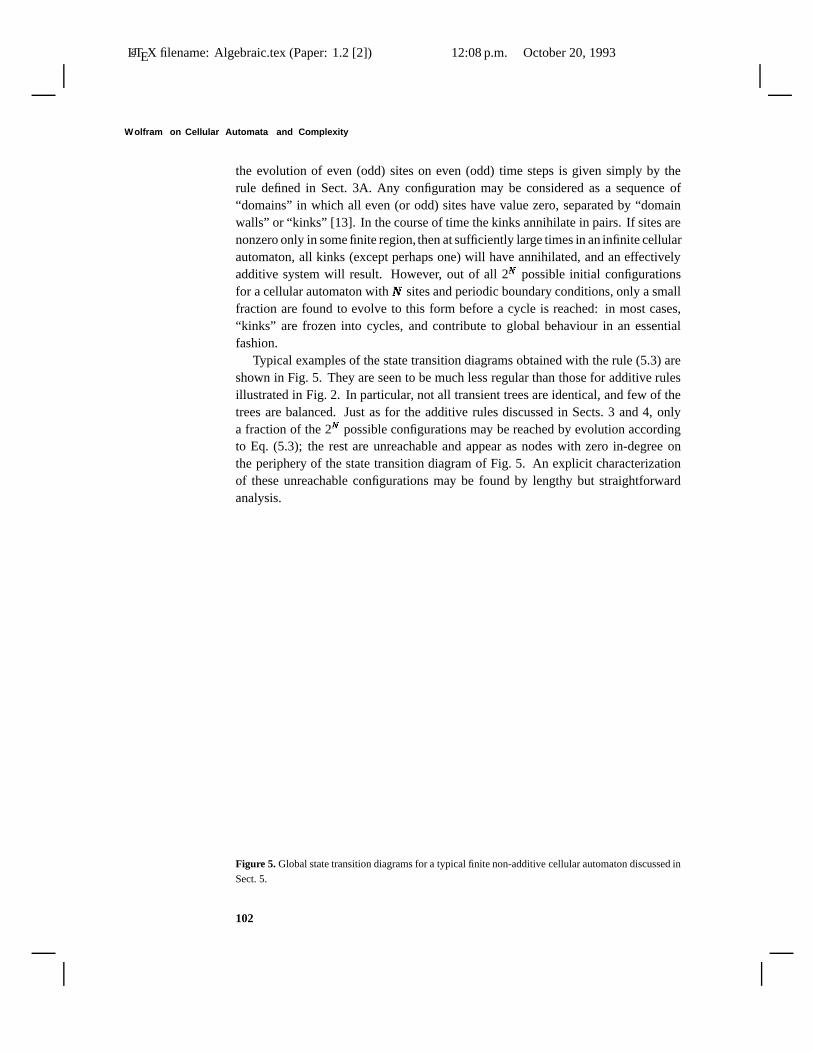
LaTEX filename: Algebraic.tex (Paper: 1.2 [2]) 12:08 p.m. October 20, 1993
Wolfram on Cellular Automata and Complexity
the evolution of even (odd) sites on even (odd) time steps is given simply by therule defined in Sect. 3A. Any configuration may be considered as a sequence of“domains” in which all even (or odd) sites have value zero, separated by “domainwalls” or “kinks” [13]. In the course of time the kinks annihilate in pairs. If sites arenonzero only in some finite region, then at sufficiently large times in an infinite cellularautomaton, all kinks (except perhaps one) will have annihilated, and an effectivelyadditive system will result. However, out of all 2N
�possible initial configurations
for a cellular automaton with N�
sites and periodic boundary conditions, only a smallfraction are found to evolve to this form before a cycle is reached: in most cases,“kinks” are frozen into cycles, and contribute to global behaviour in an essentialfashion.
Typical examples of the state transition diagrams obtained with the rule (5.3) areshown in Fig. 5. They are seen to be much less regular than those for additive rulesillustrated in Fig. 2. In particular, not all transient trees are identical, and few of thetrees are balanced. Just as for the additive rules discussed in Sects. 3 and 4, onlya fraction of the 2N
�possible configurations may be reached by evolution according
to Eq. (5.3); the rest are unreachable and appear as nodes with zero in-degree onthe periphery of the state transition diagram of Fig. 5. An explicit characterizationof these unreachable configurations may be found by lengthy but straightforwardanalysis.
Figure 5. Global state transition diagrams for a typical finite non-additive cellular automaton discussed in
Sect. 5.
102

LaTEX filename: Algebraic.tex (Paper: 1.2 [2]) 12:08 p.m. October 20, 1993
Algebraic Propertiesof CellularAutomata(1984)
Lemma 5.1. A configuration is unreachable by cellular automaton time evolutionaccording to Eq. (5.3) if and only if one of the following conditions holds:
(a) The sequence of site values 111 appears.
(b) No sequence 11 appears, but the total number of 1 sites is odd.
(c) A sequence 11a� 1a� 2 ��� a� n! 11 appears, with an odd number of the a� i havingvalue 1. The two 11 sequences may be cyclically identified.
The number of reachable configurations may now be found by enumerating theconfigurations defined by Lemma 5.1. This problem is analogous to the enumerationof legal sentences in a formal language. As a simple example of the techniquesrequired (e.g. [14]), consider the enumeration of strings of N
�symbols 0 or 1 in
which no sequence 111 appears (no periodicity is assumed). Let the number of suchstrings be a. In addition, let bN
� be the number of length N�
strings containing no 111sequences in their first N
�- 1 positions, but terminating with the sequence 111. Then
(5.4a)b0 = b1 = b2 = 0 � b3 = 1 � a0 = 1 � a1 = 2 �and
2aN� = aN
�+1 + bN
�+1 (N
�‡ 0) � (5 � 4b)
aN� = bN
�+1 + bN
�+2 + bN
�+3 (N
�‡ 0) � (5 � 4c)
The recurrence relations (5.4) may be solved by a generating function technique.With
(5.5a)A(z? ) =¥
n! =0
an! z? n! � B (z? ) =¥
n! =0
bn! z? n! �Eq. (5.4) may be written as
2A(z? ) = z? - 1(A(z? ) - 1) + z? - 1B (z? ) �A(z? ) = z? - 3B (z? ) + z? - 2B (z? ) + z? - 1B (z? ) �
Solving these equations yields the result
(5.5b)A(z? ) =1 + z? + z? 2
1 - z? - z? 2 - z? 3 �Results for specific N
�are obtained as the coefficients of z? N
�in a series expansion of
A(z? ). Taking
A(z? ) =A N� (z? )
A D (z? ) �Eq. (5.5a) may be inverted to yield
(5.5c)aN� =
i
�- A N
� (z? i)
z? i A HD (z? i )�(1�z? i)
N��
103

LaTEX filename: Algebraic.tex (Paper: 1.2 [2]) 12:08 p.m. October 20, 1993
Wolfram on Cellular Automata and Complexity
where the z? i are the roots of A D (z? ) (all assumed distinct), and prime denotes differ-entiation. This yields finally
(5.6)aN� ƒ 1 � 14(1 � 84)N
�+ 0 � 283(0 � 737)N
�cos(2 � 176N
�+ 2 � 078) �
The behaviour of the coefficients for large N�
is dominated by the first term, associatedwith the smallest root of A D (N
�). The first ten values of aN
� are 1, 2, 4, 7, 13, 24, 44,81, 149, 274, 504.
A lengthy calculation shows that the number of possible strings of length N�
which do not satisfy the conditions in Lemma 5.1, and may therefore be reached byevolution of the cellular automaton defined by Eq. (5.3), is given as the coefficientof z? N
�in the expansion of the generating function
P (z? ) =z? - 3z? 2 + 6z? 3 - 8z? 4 + 4z? 5 - z? 7
1 - 4z? + 6z? 2 - 5z? 3 + 2z? 4 + z? 5 - z? 6 + z? 7
=3 - 4z? + z? 2
1 - 2z? + z? 2 - z? 3-
2 - z?2(1 - z? + z? 2)
+2 - z?
2(- 1 + z? + z? 2)- 1 � (5 � 7)
Inverting according to Eq. (5.5c), the number of reachable configurations of lengthN�
is given by
(5.8)r N� = kN
�- (f N
�+ (-f) - N
�) - cos(N
�p�3) + 2mN
�cos(N
�q) �
where k ƒ 1 � 7548 is the real root of z? 3 - z? 2 + 2z? - 1 = 0, f = (1 + I 5)�2 = 1 � 6182,
and mƒ 0 � 754, q ƒ 1 � 408. The first ten values of r N� are 1, 1, 4, 7, 11, 19, 36, 67, 121,
216. For large N�
, r N� …kN
�. Equation (5.8) shows that corrections decrease rapidly
and smoothly with N�
. This behaviour is to be contrasted with the irregular behaviouras a function of N
�found for additive cellular automata in Theorems 3.1 and 4.2.
Equation (5.8) shows that the fraction of all 2N�
possible configurations which arereachable after one time step in the evolution of the cellular automaton of Eq. (5.2)is approximately (k
�2)N�
ƒ 0 � 92N�
. Thus, starting from an initial maximal entropyensemble with s� = 1, evolution for one time step according to Eq. (5.2) yields a setentropy
(5.9)s� (t� = 1) ƒ log2 k ƒ 0 � 88 �The irregularity of the transient trees illustrated in Fig. 5 implies a measure entropys� m< s� .
The result (5.9) becomes exact in the limit N�
¢ ¥ . A direct derivation in thislimit is given in [17, 18], where it is also shown that the set of infinite configurationsgenerated forms a regular formal language. The set continues to contract with time,so that the set entropy decreases below the value given by Eq. (5.9) [18].
Techniques similar to those used in the derivation of Eq. (5.5) may in principlebe used to deduce the number of configurations reached after any given number ofsteps in the evolution of the cellular automaton (5.2). The fraction of configurations
104

LaTEX filename: Algebraic.tex (Paper: 1.2 [2]) 12:08 p.m. October 20, 1993
Algebraic Propertiesof CellularAutomata(1984)
N r ¥N�
4 0.31255 0.34386 0.10947 0.00788 0.11339 0.1426
10 0.079111 0.043512 0.046613 0.035014 0.016315 0.0030816 0.0085017 0.00857
Table 3. Fraction of configurations appearing in cycles for the non-additive
cellular automaton of Eq. (5.2).
which appear in cycles is an irregular function of N�
; some results for small N�
aregiven in Table 3.
6. Discussion
The analysis of additive cellular automata in Sects. 3 and 4 yielded results on theglobal behaviour of additive cellular automata more complete than those availablefor most other dynamical systems. The extensive analysis was made possible bythe discrete nature of cellular automata, and by the additivity property which led tothe algebraic approach developed in Sect. 3. Similar algebraic techniques should beapplicable to some other discrete dynamical systems.
The analysis of global properties of cellular automata made in this paper comp-lements the analysis of local properties of ref. [1].
One feature of the results on additive cellular automata found in Sects. 3 and 4, isthe dependence of global quantities not only on the magnitude of the size parameterN�
, but also on its number theoretical properties. This behaviour is shared by manydynamical systems, both discrete and continuous. It leads to the irregular variationof quantities such as cycle lengths with N
�, illustrated in Table 1 and Fig. 3. In
physical realizations of cellular automata with large size N�
, an average is presumablyperformed over a range of N
�values, and irregular dependence on N
�is effectively
smoothed out. A similar irregular dependence is found on the number k
of possiblevalues for each site: simple results are found only when k
is prime.
Despite such detailed dependence on N�
, results such as Theorems 4.1–4.3 showthat global properties of additive cellular automata exhibit a considerable universality,and independence of detailed aspects of their construction. This property is againshared by many other dynamical systems. It potentially allows for generic results,valid both in the simple cases which may easily be analysed, and in the presumablycomplicated cases which occur in real physical systems.
105

LaTEX filename: Algebraic.tex (Paper: 1.2 [2]) 12:08 p.m. October 20, 1993
Wolfram on Cellular Automata and Complexity
The discrete nature of cellular automata makes possible an explicit analysis oftheir global behaviour in terms of transitions in the discrete phase space of theirconfigurations. The results of Sect. 4 provide a rather complete characterizationof the structure of the state transition diagrams for additive cellular automata. Thestate transition diagrams consist of trees corresponding to irreversible “transients”,leading to “attractors” in the form of distinct finite cycles. The irreversibility ofthe cellular automata is explicitly manifest in the convergence of several distinctconfigurations to single configurations through motion towards the roots of the trees.This irreversibility leads to a decrease in the entropy of an initially equiprobableensemble of cellular automaton configurations; the results of Sect. 4 show that inmost cases the entropy decreases by a fixed amount at each time step, reflectingthe balanced nature of the trees. Theorem 4.3 gives an algebraic characterizationof the magnitude of the irreversibility, in terms of the in-degrees of nodes in thetrees. The length of the transients during which the entropy decreases is given bythe height of the trees in Theorem 4.3, and is found always to be less than N
�. After
these transients, any initial configurations evolve to configurations on attractors orcycles. Theorem 4.3 gives the total number of configurations on cycles in terms ofN�
and algebraic properties of the cellular automaton time evolution polynomial. Atone extreme, all configurations may be on cycles, while at the other extreme, allinitial configurations may evolve to a single limit point consisting simply of the nullconfiguration.
Theorem 4.1 gives a rather general result on the lengths of cycles in additivecellular automata. The maximum possible cycle length is found to be of orderthe square root of the total number of possible configurations. Rather long cyclesare therefore possible. No simple results on the total number of distinct cycles orattractors were found; however, empirical results suggest that most cycles have alength equal to the maximal length for a particular cellular automaton.
The global properties of additive cellular automata may be compared with those ofother mathematical systems. One closely related class of systems are linear feedbackshift registers. Most results in this case concentrate on analogues of the cellularautomaton discussed in Sect. 3, but with the values at a particular time step in generaldepending on those of a few far-distant sites. The boundary conditions assumedfor feedback shift registers are typically more complicated than the periodic onesassumed for cellular automata in Sect. 3 and most of Sect. 4. The lack of symmetryin these boundary conditions allows for maximal length shift register sequences, inwhich all 2N
�- 1 possible configurations occur on a single cycle [2, 3].
A second mathematical system potentially analogous to cellular automata is arandom mapping [15]. While the average cycle length for random mappings iscomparable to the maximal cycle length for cellular automata, the probability fora node in the state transition diagram of a random mapping to have in-degree d
0is
…1�d0
!, and is much more sharply peaked at low values than for a cellular automaton,leading to many differences in global properties.
106

LaTEX filename: Algebraic.tex (Paper: 1.2 [2]) 12:08 p.m. October 20, 1993
Algebraic Propertiesof CellularAutomata(1984)
Non-additive cellular automata are not amenable to the algebraic techniques usedin Sects. 3 and 4 for the additive case. Section 5 nevertheless discussed some prop-erties of non-additive cellular automata, concentrating on a simple one-dimensionalexample with two possible values at each site. Figure 5 indicates that the state transi-tion diagrams for such non-additive cellular automata are less regular than those foradditive cellular automata. Combinatorial methods were nevertheless used to derivethe fraction of configurations with no predecessors in these diagrams, giving theirreversibility and thus entropy decrease associated with one time step in the cellularautomaton evolution. Unlike the case of additive cellular automata, the result wasfound to be a smooth function of N
�.
Appendix A:Notations and Elementar y Results on Finite Fields
Detailed discussion of the material in this appendix may be found in [8].
A. Basic Notations
a� mod bJ
denotes a� reduced modulo bJ
, or the remainder of a� after division by bJ
.(a� � bJ ) or gcd(a� � bJ ) denotes the greatest common divisor of a� and b
J. When a� and
bJ
are polynomials, the result is taken to be a polynomial with unit leading coefficient(monic).
a� � bJ represents the statement that a� divides bJ
(with no remainder).a� n! 2 bJ indicates that a� n! is the highest power of a� which divides b
J.
Exponentiation is assumed right associative, so that a� bK c
denotes a� (bK c) not (a� b
K)cL .
p usually denotes a prime integer.Ùk� denotes an arbitrary commutative ring of k
elements.
Úk� denotes the ring of integers modulo k
.
degP (x� ) denotes the highest power of x� which appears in P (x� ).
B. Finite Fields
There exists a finite field unique up to isomorphism with any size p a (p prime),denoted GF(p a). p is termed the characteristic of the field.
The ring Úk� of integers modulo k
forms a field only when k
is prime, since only
in this case do unique inverses under multiplication modulo k
exist for all nonzeroelements. (For example, in Ú4, 2 has no inverse.) GF(p ) is therefore isomorphicto Úp4 .
The field GF(p a) is conveniently represented by the set of polynomials of degreeless than a with coefficients in Úp4 , with all polynomial operations performed moduloa fixed irreducible polynomial of degree a over GF(p ). For example, GF(4) maybe represented by elements 0, 1, k, k + 1 with operations performed modulo 2 andmodulo k2 + k + 1. In this case for example k · k ” k + 1. Notice that, as mentionedin Sect. A.C below, polynomials over a field form a unique factorization domain.
107

LaTEX filename: Algebraic.tex (Paper: 1.2 [2]) 12:08 p.m. October 20, 1993
Wolfram on Cellular Automata and Complexity
Any field of size qM yields a group of size qM - 1 under multiplication if the zeroelement is removed. Thus for any element of GF(qM ),
(A.1)x� qN = x� �and x� qN - 1 = 1 for x� „ 0. Notice that if x� ¸ GF(p a) and x� p4 b
= x� , then x� ¸ GF(p b).
C. Polynomials over Finite Fields
Polynomials in any number of variables with coefficients in GF(qM ) form a unique fac-torization domain. For such polynomials, therefore, A(x� )B (x� ) ” A(x� )C(x� ) mod P (x� )implies B (x� ) ” C(x� ) mod P (x� ) if (A(x� ), P (x� )) = 1.
For any polynomials A(x� ) and B (x� ) with coefficients in GF(qM ), there exist poly-nomials a(x� ) and b(x� ) such that
(A.2)C(x� ) = (A(x� ) � B (x� )) = a(x� )A(x� ) + b(x� )B (x� ) �There are exactly qM n! univariate polynomials over GF(qM ) with degree less than n" .
With a polynomial Q (x� ) of degree m� , the number of polynomials P (x� ) with degreenot exceeding n" for which Q (x� ) � P (x� ) is qM n! - m� for m� £ n" .
For any prime p , and for elements a� i of GF(p b),
(A.3)� a� i x� i �
p4 a
= (a� ix� i )p4 a �
Thus for example,
(A.4)(x� 2a+ 1) ” (x� + 1)2a
mod 2 �a result used extensively in Sect. 3.
If P (x� ) � Q (x� ), then every root of P (x� ) must be a root of Q (x� ). If l ‡ 2 and
(A.5)[P (x� )] l � Q (x� ) �then
(A.6)P (x� ) � Q H (x� ) �where Q H (x� ) is the formal derivative of Q (x� ), obtained by differentiation of each termin the polynomial. [Note that integration is not defined for polynomials over GF(qM ).]
The number of roots (not necessarily distinct) of a polynomial over GF(qM ) is equalto the degree of the polynomial. The roots may lie in an extension of GF(qM ).
Over the field GF(p ),
(A.7)x� N�
- 1 = (x� n! - 1)Dp (N�
) �where N
�= Dp4 (N
�)n" , with Dp4 (N
�) defined in Sects. 3 and 4 as the maximum power of
p which divides N�
. The polynomial x� n! - 1 with n" not a multiple of p then factorizesover GF(p ) according to
(A.8)x� n! - 1 = (x� - 1)d)+*
n!d)
„ 1
f( d )ordd (p )
i=1
Cd)-,
i (x� ) �
108

LaTEX filename: Algebraic.tex (Paper: 1.2 [2]) 12:08 p.m. October 20, 1993
Algebraic Propertiesof CellularAutomata(1984)
where the Cd),
i (x� ) are irreducible cyclotomic polynomials of degree ordd
) (p ). Notethat the multiplicity of any irreducible factor of x� N
�- 1 is exactly Dp4 (N
�), and that
(A.9)Cd)-,
i (x� ) � x� d
)- 1 �
D. Dipolynomials over Finite Fields
A dipolynomial A(x� ) is taken to divide a dipolynomial B (x� ) if there exists a dipolyno-mial C(x� ) such that B (x� ) = A(x� )C(x� ). Hence if A(x� ) and B (x� ) are polynomials, withA(0) „ 0, and if A(x� ) � B (x� ) are dipolynomials, then A(x� ) � B (x� ) are polynomials.
Congruence in the ring of dipolynomials is defined as follows: A(x� ) ” B (x� ) modC(x� ) for dipolynomials A(x� ), B (x� ), and C(x� ) if C(x� ) � A(x� ) - B (x� ).
The greatest common divisor of two nonzero dipolynomials A 1(x� ) and A 2(x� ) isdefined as the ordinary polynomial (A �1(x� ) � A �2(x� )), where A �i (x� ) = x� m� i A i (x
� ) and m� i ischosen to make A �i (x� ) a polynomial with nonzero constant term. Note that by analogywith Eq. (A.2), for any dipolynomials A 1(x
� ) and A 2(x� ), there exist dipolynomialsa1(x� ) and a2(x� ) such that
(A.10)(A 1(x� ) � A 2(x� )) = a1(x� )A 1(x� ) + a2(x
� )A 2(x� ) �Appendix B:Proper ties and Values of Some NumberTheoretical Functions
A. Euler Totient Function @%N &
f( N�
) is defined as the number of integers less than N�
which are relatively prime toN�
[7]. f( N�
) is a multiplicative function, so that
(B.1)f( m� n" ) = f( m� )f( n" ) � (m� � n" ) = 1 �For p prime,
(B.2)f( p a) = p a- 1(p - 1) �Hence
(B.3)f( n" ) =p4 a O n! p a- 1(p - 1) �
providing a formula by which f( N�
) may be computed. Some values of f( N�
) aregiven in Table 4.
f( N�
) is bounded (for N�
> 1) by
(B.4)c@ N�C�
log log N�
£ f( N�
) £ N�
- 1 �where c@ is some positive constant, and the upper bound is achieved if and only if N
�is prime. For large N
�, f( N
�)�N�
tends on average to a constant value.f( n" ) satisfies the Euler-Fermat theorem
(B.5)k f( n! ) = 1 mod n" (k
� n" ) = 1 �
109

LaTEX filename: Algebraic.tex (Paper: 1.2 [2]) 12:08 p.m. October 20, 1993
Wolfram on Cellular Automata and Complexity
B. Multiplicative Order Function ord N %k &
The multiplicative order function ordN� (k ) is defined as the minimum positive integer
j�
for which [8]
(B.6)k j�
= 1 mod N� �
This condition can only be satisfied if (k � N� ) = 1.
By the Euler-Fermat theorem (B.5),
(B.7)ordN� (k ) � f( N
�)
In addition, ordm� n! (k ) = lcm(ordn! (k ), ordm� (k
)), (n" � k ) = (m� � k ) = (n" � m� ) = 1. Some
special cases are
ordk�
a- 1(k ) = a �
ordk�
a+1(k ) = 2a �
A rigorous bound on ordN� (k ) is
(B.8)logk� (N� ) £ ordN
� (k ) £ N
�- 1 �
where the upper bound is attained only if N�
is prime. It can be shown that onaverage, for large N
�, ordN
� (k ) ½I N
�; the actual average is presumably closer to N
�.
Nevertheless, for large N�
, ordN� (k )�N�
tends to zero on average.Some values of the multiplicative order function are given in Table 4.The multidimensional generalization ordN
�1, = = = ,
N�
d(k ) of the multiplicative order
function is defined as the minimum positive integer j�
for which k j�
= 1 simultaneouslymodulo N
�1, N�
2 ������ and N�
d) . It is clear that
ordN�
1, = = = ,
N�
d(k ) = lcm(ordN
�1(k ) ����� ordN
�d(k )) = ordlcm(N
�1, = = = ,
N�
d )(k ) �
(k � N� 1) = ���� = (k
� N� d) ) = 1 � (B � 9)
C. Multiplicative Suborder Function sord N %k &
The multiplicative suborder function is defined as the minimum j�
for which
(B.10)k j�
= –1 mod N� �
again assuming (k � N� ) = 1. Comparison with (B.6) yields
(B.11a)sordN� (k ) = ordN
� (k ) �
or
(B.11b)sordN� (k ) = 1
2 ordN� (k ) �
The second case becomes comparatively rare for large N�
; the fraction of integers lessthan X for which it is realised may be shown to be asymptotic to c@ � [log X ] l [16],where c@ and l are constants determined by k
.
110

LaTEX filename: Algebraic.tex (Paper: 1.2 [2]) 12:08 p.m. October 20, 1993
Algebraic Propertiesof CellularAutomata(1984)
N k = 2 k = 3 k = 4 k = 5 f( N )
1 12 1 1 1 1 13 2 1 1 1 2 1 24 2 1 1 1 25 4 2 4 2 2 1 46 2 1 27 3 3 6 3 3 3 6 3 68 2 2 2 2 49 6 3 3 3 6 3 6
10 4 2 411 10 5 5 5 5 5 5 5 1012 2 2 413 12 6 3 3 6 3 4 2 1214 6 3 6 3 615 4 4 2 2 816 4 4 4 4 817 8 4 16 8 4 2 16 8 1618 6 3 619 18 9 18 9 9 9 9 9 1820 4 4 821 6 6 3 3 6 3 1222 5 5 5 5 1023 11 11 11 11 11 11 22 11 2224 2 2 825 20 10 20 10 10 5 2026 3 3 4 2 1227 18 9 9 9 18 9 1828 6 3 6 6 1229 28 14 28 14 14 7 14 7 2830 831 5 5 30 15 5 5 3 3 3032 8 8 8 8 1633 10 5 5 5 10 10 2034 16 8 16 8 1635 12 12 12 12 6 6 2436 6 6 1237 36 18 18 9 18 9 36 18 3638 18 9 9 9 1839 12 12 6 6 4 4 2440 4 4 16
Table 4. Values of the multiplicative order ordN� (k$
) and suborder sordN� (k$
) functions defined in
Eqs. (B.6) and (B.10), respectively, together with values of the Euler totient function f(N ). Each column
gives values of the pair ordN� (k$
), sordN� (k$
).
111

LaTEX filename: Algebraic.tex (Paper: 1.2 [2]) 12:08 p.m. October 20, 1993
Wolfram on Cellular Automata and Complexity
In general,
(B.12)logk� (N� ) £ sordN
� (k ) £ (N
�- 1)
�2 �
the upper limit again being achieved only if N�
is prime. For large N�
, sordN� (k )�N�
¢ 0on average.
The multidimensional generalization sordN�
1, = = = ,
N�
d(k ) of the multiplicative suborder
function is defined as the minimum positive integer j�
for which k j�
= –1 simultane-ously modulo N
�1 ������� N� d
) , with +1 and - 1 perhaps taken variously for the differentN�
i . The analogue of Eq. (B.9) for this function is
(B.13a)sordN�
1, = = = ,
N�
d(k ) = lcm(sordN
�1(k ) ����� sordN
�d(k )) �
and
(B.13b)lcm(sordN�
1(k ) �3����� sordN
�d(k )) = sord lcm(N
�1, = = = ,
N�
d )(k ) �
or
(B.13c)lcm(sordN�
1(k ) �3����� sordN
�d(k )) = 1
2 sord lcm(N�
1, = = = ,
N�
d )(k ) �
Acknowledgement. We are grateful to O. E. Lanford for several suggestions.
References
1. Wolfram, S.: Statistical mechanics of cellular automata. Rev. Mod. Phys. 55, 601 (1983).
2. Golomb, S.W.: Shift register sequences. San Francisco: Holden-Day 1967.
3. Selmer, E.S.: Linear recurrence relations over finite fields. Dept. of Math., Univ. of Bergen,Norway (1966).
4. Miller, J.C.P.: Periodic forests of stunted trees. Phil. Trans. R. Soc. Lond. A266, 63 (1970);A293, 48 (1980).ApSimon, H.G.: Periodic forests whose largest clearings are of size 3. Phil. Trans. R. Soc. Lond.A266, 113 (1970).ApSimon, H.G.: Periodic forests whose largest clearings are of size nP ‡ 4. Proc. R. Soc. Lond.A319, 399 (1970).Sutton, C.: Forests and numbers and thinking backwards. New Sci. 90, 209 (1981).
5. Moore, E.F.: Machine models of self-reproduction. Proc. Symp. Appl. Math. 14, 17 (1962)reprinted in: Essays on cellular automata, A. W. Burks. Univ. of Illinois Press (1966).Aggarwal, S.: Local and global Garden of Eden theorems. Michigan University technical rept.147 (1973).
6. Knuth, D.: Fundamental algorithms, Reading, MA: Addison-Wesley 1968.
7. Hardy, G.H., Wright, E.M.: An introduction to the theory of numbers. Oxford: Oxford UniversityPress 1968.
8. MacWilliams, F.J., Sloane, N.J.A.: The theory of error-correcting codes. Amsterdam: North-Holland 1977.
9. Griffiths, P., Harris, J.: Principles of algebraic geometry. New York: Wiley 1978.
10. Fredkin, E., Margolus, N.: Private communications.
112

LaTEX filename: Algebraic.tex (Paper: 1.2 [2]) 12:08 p.m. October 20, 1993
Algebraic Propertiesof CellularAutomata(1984)
11. Ronse, C.: Non-linear shift registers: A survey. MBLE Research Lab. report, Brussels (May1980).
12. Harao, M. and Noguchi, S.: On some dynamical properties of finite cellular automaton. IEEETrans. Comp. C-27, 42 (1978).
13. Grassberger, P.: A new mechanism for deterministic diffusion. Phys. Rev. A (to be published).
14. Guibas, L.J., Odlyzko, A.M.: String overlaps, pattern matching, and nontransitive games. J.Comb. Theory (A) 30, 83 (1981).
15. Knuth, D.: Seminumerical algorithms. 2nd ed. Reading, MA: Addison-Wesley 1981.Gelfand, A.E.: On the cyclic behavior of random transformations on a finite set. Tech. rept. 305,Dept. of Statistics, Stanford Univ. (August 1981).
16. Odlyzko, A.M.: Unpublished.
17. Lind, D.A.: Applications of ergodic theory and sofic systems to cellular automata. Physica D 10(to be published).
18. Wolfram, S.: Computation theory of cellular automata. Institute for Advanced Study preprint(January 1984).
19. Lenstra, H.W., Jr.: Private communication.
113