algebraic real analysis - mount allison university · algebraic real analysis 217 denote a...

Theory and Applications of Categories, Vol. 20, No. 10, 2008, pp. 215–306.

ALGEBRAIC REAL ANALYSIS

PETER FREYD

Abstract. An effort to initiate the subject of the title: the basic tool is the study ofthe abstract closed interval equipped with certain equational structures.

The title is wishful thinking; there ought to be a subject that deserves the name“algebraic real analysis.”

Herein is a possible beginning.For reasons that can easily be considered abstruse we were led to the belief that the

closed interval—not the entire real line—is the basic structure of interest. Before describingthose abstruse reasons, a theorem:

Let G be a compact group and I the closed interval. (We will not say which closedinterval; to do so would define it as a part of the reals, belying the view of the closedinterval as the fundamental structure.) Let C(G) be the set of continuous maps from G toI. We wish to view this as an algebraic structure, where the word “algebra” is in the verygeneral sense, something described by operations and equations. In the case at hand, theonly operators that will be considered right now are the constants, “top” and “bottom,”denoted > and ⊥, and the binary operation of “midpointing,” denoted x|y. (There areaxioms that will define the notion of “closed midpoint algebra” but since the theorem isabout specific examples they’re not now needed.) C(G) inherits this algebraic structure inthe usual way (f |g, for example, is the map that sends σ ∈ G to (fσ)|(gσ) ∈ I). We use thegroup structure on G to define an action of G on C(G), thus obtaining a representation of Gon the group of automorphisms of the closed midpoint algebra. (Fortunately no knowledgeof the axioms is necessary for the definition of automorphism, or even homomorphism.)Let (C(G),I) be the set of closed-midpoint-algebra homomorphisms from C(G) to I. Againwe obtain an action of G.

0.1. Theorem. There is a unique G-fixed point in (C(G),I)

There is an equivalent way of stating this:

Special thanks to Mike Barr and Don von Osdol for editorial assistance and to the Executive Directorof the FMS Foundation for making it all possible.

Received by the editors 2008-02-09 and, in revised form, 2008-06-25.Transmitted by Michael Barr. Published on 2008-07-02.2000 Mathematics Subject Classification: 03B45, 03B50, 03B70, 03D15, 03F52, 03F55, 03G20, 03G25,

03G30, 08A99, 18B25, 18B30, 18F20, 26E40, 28E99, 46M99, 34A99.Key words and phrases: algebraic real analysis, closed interval, closed midpoint algebra, chromatic

scale, coalgebraic real analysis, complete scale, finitely presented scale, free scale, harmonic scale, injectivescale, lattice-ordered abelian group, linear logic, Lipschitz extension, Lukasiewicz logic, midpoint algebra,minor scale, modal logic, ordered wedge, scale, semi-simple scale, simple scale, zoom operator.

c© Peter Freyd, 2008. Permission to copy for private use granted.

215

216 PETER FREYD

0.2. Theorem. There is a unique G-invariant homomorphism from the closed midpointalgebra C(G) to I.

This theorem is mostly von Neumann’s: the unique G-invariant homomorphism isintegration, that is, it is the map that sends f : G → I to

∫f dσ. But it is not entirely

von Neumann’s: we have just characterized integration on compact groups without a singlemention of inequalities or limits. The only non-algebraic notion that appeared was at thevery beginning in the definition of C(G) as the set of continuous maps (in time we willobtain a totally algebraic definition).

The fact that we are stating this theorem for I and not the reals, R is critical. Considerthe special case when G is the one-element group; the theorem says that the identity mapon I is the only midpoint-preserving endomorphism that fixes > and ⊥ (we said thatthe theorem is mostly von Neumann’s; this part is not). It actually suffices to assumethat the endomorphism fixes any two points but with the axiom of choice and a standardHamel-basis argument we can find 22ℵ0 counterexamples for this assertion if I is replacedwith R.

We do not need a group structure or even von Neumann to make the point. Con-sider this remarkably simple characterization of definite integration on C(I), continuousfunctions from I to I:

∫

∫> dx = > ∫

∫⊥ dx = ⊥

∫

∫f(x) | g(x) dx = ∫

∫f(x) dx | ∫

∫g(x) dx

∫

∫f(x) dx = ∫

∫f(⊥|x) dx | ∫

∫f(x|>) dx [1]

No inequalities. No limits. The first three equations say just that integration is ahomomorphism of closed midpoint algebras. The fourth equation says that the meanvalue of a function on I is the midpoint of the two mean-values of the function on thetwo halves of I.

The fourth equation—as any numerical or theoretical computer scientist will tell you—is a “fixed-point characterization.” When Church proved that his and Godel’s notion ofcomputability were coextensive he used the fact that all computation can be reduced tofinding fixed points. (The word “point” here is traditional but misleading. The fixed pointunder consideration here is, as it was for Church, an operator on functions—rather farremoved from the public notion of point.)

If we seek a fixed point of an operator the first thing to try, of course, is to iterate theoperator on some starting point and to hope that the iterations converge. So let

∫

∫0

f(x) dx

1There was an appendix for Latex macros, but the powers that be deemed such to be beneath thedignity of this journal.

ALGEBRAIC REAL ANALYSIS 217

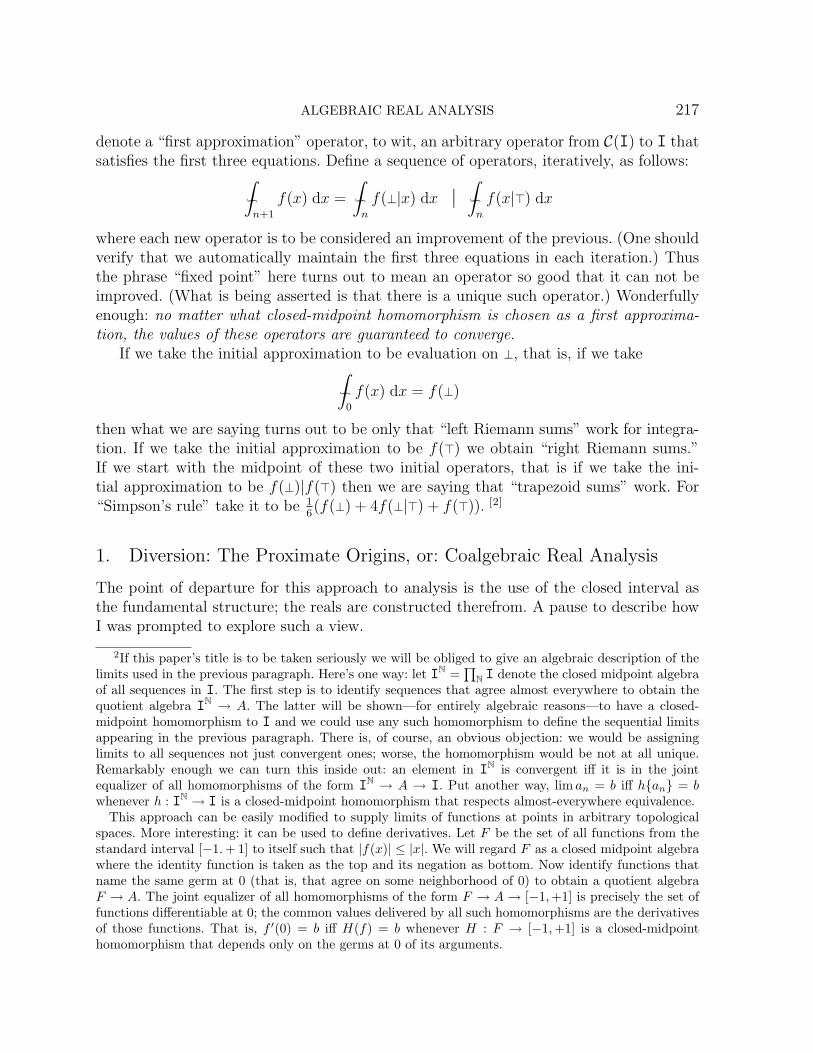
denote a “first approximation” operator, to wit, an arbitrary operator from C(I) to I thatsatisfies the first three equations. Define a sequence of operators, iteratively, as follows:

∫

∫n+1

f(x) dx = ∫

∫n

f(⊥|x) dx | ∫

∫n

f(x|>) dx

where each new operator is to be considered an improvement of the previous. (One shouldverify that we automatically maintain the first three equations in each iteration.) Thusthe phrase “fixed point” here turns out to mean an operator so good that it can not beimproved. (What is being asserted is that there is a unique such operator.) Wonderfullyenough: no matter what closed-midpoint homomorphism is chosen as a first approxima-tion, the values of these operators are guaranteed to converge.

If we take the initial approximation to be evaluation on ⊥, that is, if we take∫

∫0

f(x) dx = f(⊥)

then what we are saying turns out to be only that “left Riemann sums” work for integra-tion. If we take the initial approximation to be f(>) we obtain “right Riemann sums.”If we start with the midpoint of these two initial operators, that is if we take the ini-tial approximation to be f(⊥)|f(>) then we are saying that “trapezoid sums” work. For“Simpson’s rule” take it to be 1

6(f(⊥) + 4f(⊥|>) + f(>)). [2]

1. Diversion: The Proximate Origins, or: Coalgebraic Real Analysis

The point of departure for this approach to analysis is the use of the closed interval asthe fundamental structure; the reals are constructed therefrom. A pause to describe howI was prompted to explore such a view.

2If this paper’s title is to be taken seriously we will be obliged to give an algebraic description of thelimits used in the previous paragraph. Here’s one way: let IN =

∏N I denote the closed midpoint algebra

of all sequences in I. The first step is to identify sequences that agree almost everywhere to obtain thequotient algebra IN → A. The latter will be shown—for entirely algebraic reasons—to have a closed-midpoint homomorphism to I and we could use any such homomorphism to define the sequential limitsappearing in the previous paragraph. There is, of course, an obvious objection: we would be assigninglimits to all sequences not just convergent ones; worse, the homomorphism would be not at all unique.Remarkably enough we can turn this inside out: an element in IN is convergent iff it is in the jointequalizer of all homomorphisms of the form IN → A → I. Put another way, lim an = b iff han = bwhenever h : IN → I is a closed-midpoint homomorphism that respects almost-everywhere equivalence.

This approach can be easily modified to supply limits of functions at points in arbitrary topologicalspaces. More interesting: it can be used to define derivatives. Let F be the set of all functions from thestandard interval [−1. + 1] to itself such that |f(x)| ≤ |x|. We will regard F as a closed midpoint algebrawhere the identity function is taken as the top and its negation as bottom. Now identify functions thatname the same germ at 0 (that is, that agree on some neighborhood of 0) to obtain a quotient algebraF → A. The joint equalizer of all homomorphisms of the form F → A → [−1, +1] is precisely the set offunctions differentiable at 0; the common values delivered by all such homomorphisms are the derivativesof those functions. That is, f ′(0) = b iff H(f) = b whenever H : F → [−1, +1] is a closed-midpointhomomorphism that depends only on the germs at 0 of its arguments.

218 PETER FREYD

The community of theoretical computer scientists (in the European sense of the phrase)had found something called “initial-algebra” definitions of data types to be of great use.Such definitions typically tell one how inductive programs—and then recursive programs—are to be defined and executed. It then became apparent that some types were betterhandled in a dual fashion: something called “final-coalgebra” definitions. Such can tellone how “co-inductive” and “co-recursive” programs are to be defined and executed.(One must really resist here the temptation to say “co-defined” and “co-executed.”)

Thus began a search for a final-coalgebra definition of that ancient data type, the reals.There is, actually, always a trivial answer to the question: every object is automaticallythe final coalgebra of the functor constantly equal to that object. What was being soughtwas not just a functor with a final coalgebra isomorphic to the object in question but afunctor that supplies its final coalgebra with the structure of interest. In 1999 an answerwas found not for the reals but for the closed interval.[3] (To this date, no one has founda functor whose final coalgebra is usefully the reals.)

Consider, then, the category whose objects are sets with two distinguished points, topand bottom, denoted T and

T

and whose maps are the functions that preserve > and ⊥.Given a pair of objects, X and Y , we define their ordered wedge, denoted X ∨ Y tobe the result of identifying the top of X with the bottom of Y. [4] This construction canclearly be extended to the maps to obtain the “ordered-wedge functor.”

The closed interval can be defined as the final coalgebra of the functor that sends Xto X ∨X. Let me explain.

First (borrowing from the topologists’ construction of the ordinary wedge), X ∨ Y istaken as the subset of pairs, 〈x, y〉, in the product X × Y that satisfy the disjunctivecondition: x = > or y = ⊥. A map, then, from X to X ∨ X may be construed as

a pair of self-maps, denoted∧x and

∨x, such that for all x either

∨x = > or

∧x = ⊥.

The final coalgebra we seek is the terminal object in the category whose objects arethese structures.[5] To be formal, begin with the category whose objects are quintuples〈X,⊥,>, ∧, ∨〉 where ⊥,> ∈ X, and ∧, ∨ signify self-maps on X. The maps of the categoryare the functions that preserve the two constants and the two self-maps. Then cut downto the full subcategory of objects that satisfy the conditions:

∧> = > =

∨>

∧⊥ = ⊥ =

∨⊥

∀x [∧x = ⊥ or

∨x = >]

⊥ 6= > [6]

3First announced in a note I posted on 22 December, 1999, http://www.mta.ca/∼cat-dist/1999/99-124The word “wedge” and its notation are borrowed from algebraic topology where X ∨ Y is the result

of joining the (single) base-point of X to that of Y .5This is the specialization of the general notion: given an endofunctor T , a “T -coalgebra” is just a

map X → TX.6I did not say “with a pair of distinguished points” above. What I said was “with two distinguished

points”

We will call such a structure an interval coalgebra.[7]

I said that we will eventually construct the reals from I. But if one already has thereals then one may chose ⊥ < > and define a coalgebra structure on [⊥,>] as

∨x = min(2x− ⊥,>)

∧x = max(2x− >,⊥)

Note that each of the two self-maps evenly expands a half interval to fill the entireinterval—one the bottom half the other the top half. We will call them zoom operators.(By convention we will not say “zoom in” or “zoom out.” All zooming herein is expansive,not contractive.)

The general definition of “final coalgebra” reduces—in this case—to the characteriza-tion of such a closed interval, I, as the terminal object in this category.[8]

The general notion of “co-induction” reduces—in this case—to the fact that given any

quintuple 〈X,⊥,>, ∧, ∨〉 satisfying the above-displayed conditions there is a unique Xf→ I

such that f(⊥) = ⊥, f(>) = >, f(∨x) = (fx)∨ and f(

∧x) = (fx)∧. If I is taken as the

unit interval, [ 0, 1], in the classical setting (and if one pays no attention to computationalfeasibility) a quick and dirty construction of f is to define the binary expansion of f(x) ∈ Iby iterating (forever) the following procedure:

If∨x = > then

emit 1 and replace x with∧x

else

emit 0 and replace x with∨x.

7The modal operations 3 for possibly and 2 for necessarily have received many formalizations butit is safe to say that no one allows simultaneously both 3Φ 6= T and 2Φ 6= T

: “less than possible butsomewhat necessary.” (The coalgebra condition can be viewed as a much weakened excluded middle:when the two unary operations are trivialized—that is, both taken to be the identity operation—then3Φ = T or 2Φ =

T

becomes just standard excluded middle.)If we assume, for the moment, that T and

T

are fixed points for 3 and 2 then we have an example

of an interval coalgebra where 2Φ is∧Φ and 3Φ is

∨Φ. The finality of I yields what may be considered

truth values for sentences (e.g. the truth value of = ⊥|> translates to “entirely possible but totallyunnecessary” and a truth value greater than >| means “necessarily entirely possible”).

The fixed-point conditions are not, in fact, appropriate—true does not imply necessarily true nor doespossibly false imply false—but, fortunately, they’re not needed: an easy corollary of the finality of I saysthat it suffices to assume the disjointness of the orbits of T and

T

under the action of the two operators.If we work in a context in which the modal operations are monotonic (that is, when Φ implies Ψ it is thecase that 2Φ implies 2Ψ and 3Φ implies 3Ψ) it suffices to assume that 2Φ implies Φ, that Φ implies3Φ and that 2nT never implies 3n T

. If this last condition has never previously been formalized it’s onlybecause no one ever thought of it.

The same treatment of modal operators holds when 3 is interpreted as tenable and 2 as certain; or 3

as conceivable and 2 as known.This topic will be much better discussed in the intuitionistic foundations considered in Section 30.8If the case with ⊥ = > were allowed then the terminal object would be just the one-point set. (In

some sense, then, the separation of > and ⊥ requires no less than an entire continuum.)

220 PETER FREYD

Note that the symmetry on I is forced by its finality: if > and ⊥ are interchanged and if>- and ⊥-zooming are interchanged the definition of interval coalgebra is maintained, hencethere is a unique map from 〈I,⊥,>, ∧, ∨〉 to 〈I,>,⊥, ∨, ∧〉 that effects those interchangesand it is necessarily an involution. It is the symmetry being sought.

The ≤ relation on I may be defined as the most inclusive binary relation preserved by ∧

and ∨ that avoids > ≤ ⊥. We will delay the (more difficult) proof that the characterizationyields a construction of the midpoint operator that figures so prominently in the opening(and throughout this work).

The assertion that the final coalgebra may be taken as the standard interval [9] needsa full proof—actually several proofs depending on the extent of constructive meaning onedesires in his notion of the standard interval (see Sections 30–32). But we move now fromthe coalgebraic theory with its disjunctive condition to an algebraic theory in the usualpurely equational sense.

2. The Equational Theory of Scales

The theory of scales is given by:a constant top

denoted >;a unary operation dotting

whose values are denoted.x ;

a unary operation >-zooming

whose values are denoted∧x and;

a binary operation midpointingwhose values are denoted x|y.

Define:the constant bottom

by ⊥ =.> ;

the constant centerby = ⊥|> and;

unary operation ⊥-zooming

by∨x =

.∧.x .

9I is also the final coalgebra of any finite iteration of ordered wedges. If we take the n-fold iteration,X ∨X ∨ · · · ∨X, as the set of n-tuples of the form 〈x0, x1, . . . , xn−1〉 such that either xi = > or xi+1 = ⊥for i = 0, 1, . . . , n−2 then the coalgebra structure is a sequence of functions z0, z1, . . . , zn−1 such thateither zi(x) = > or zi+1(x) = ⊥ for i = 0, 1, . . . , n−2. The coalgebra structure on the unit interval isgiven by zi(x) = max(0, min(1, nx− i)). Given x ∈ X obtain the base-n expansion for its correspondingelement in I by iterating (forever) the following procedure:

Let i = 0;While zi(x) = > and i < n−1 replace i with i+1;Emit i;Replace x with zi(x).

We will, when convenient, denote (x|y)∧ as x∧|y or x|y and (x|y)∨ as x

∨|y.

The equations:idempotent:

x|x = x

commutative: [10]

x|y = y|x

medial (sometimes called “middle-two interchange”): [11]

(v|w) | (x|y) = (v|x) | (w|y)

constant: [12]

.x |x =

unital: [13]

> |∧x = x = ⊥ |

∨x

And, finally, the scale identity:

u|v =∨u|∧v | ∧u|∨v

The standard model is the closed real interval IIIII of all real numbers from −1 through+1. More generally, let DDDDD be the ring of dyadic rationals (those with denominator a powerof 2). In D-modules, or as we will call them, dy-modules, with total orderings we maychoose elements ⊥ < >, and define a scale as the set of all elements from ⊥ through >

with x|y = (x + y)/2,.x= ⊥ + >− x,

∧x = max(2x−>,⊥) (hence

∨x = min(2x−⊥,>)). [14]

The standard interval in D, that is, the interval from −1 through +1, will be shown in

10This axiom can be replaced with a single instance: ⊥|> = >|⊥. See footnote below.11The medial law has a geometric interpretation: it says that the midpoints of a cycle of four edges on

a tetrahedron are the vertices of a parallelogram. That is, view four points A, B, C, D in general position inR3. Consider the closed path from A to B to D to C back to A and note that the four successive midpointsA|B, B|D, D|C, C|A appear in the medial law (A|B)|(C|D) = (A|C)|(B|D). This equation says, among otherthings, that the two line segments, the one from A|B to C|D and the one from A|C to B|D, having a pointin common, are coplanar, forcing the four midpoints, A|B, B|D, D|C, C|A to be coplanar. The medial lawsays, further, that these two coplanar line segments have their midpoints in common, And that says—indeed, is equivalent with— A|B, B|D, D|C, C|A being the vertices of a parallelogram. (A traditional proofis obtainable from the observation that two of the line segments, the one from A|B to A|C and the otherfrom D|B to D|C, are both parallel to the line segment from B to C, hence are themselves parallel.)

12A technically simpler equation is the two-variable.u |u =

.v |v.

13The commutative axiom can be removed entirely if the first (left) unital law is replaced with.⊥∧| x = x.

See Section 29.14In Sections 8 and 14 we will see that every scale has a faithful representation into a product of scales

that arise in this way.

222 PETER FREYD

the next section to be isomorphic to the initial scale (the scale freely generated by itsconstants). It will be denoted as IIIII. [15]

The verification of all but the last of the defining equations on the standard intervalis entirely routine. It will take a while before the scale identity reveals its secrets: how itfirst became known; how it can be best viewed; why it is true for the standard models.[16]

An ad hoc verification of the scale identity on the standard model may be obtainedby noting first that:

∧x =

−1 if x ≤ 0, 2x−1 if x ≥ 0

∨x =

2x+1 if x ≤ 0+1 if x ≥ 0

The scale identity then separates into four cases depending on the signatures of the twovariables. When both are positive the two sides of the identity quickly reduce to x + y− 1and, when both are negative, to −1. In the mixed case (because of commutativity weknow in advance that the two mixed cases are equivalent) where x is positive and y is

negative, the left side is, of course, (x+y2

) and the right side reduces to (−1)|(x+y). The

verification is completed therefore with the verification of z/2 = (−1)| ∧z which is, in turn,quickly verified by considering, once again, the two possible signatures of z. [17]

15The free scale on one generator will be shown in Section 20 to be isomorphic to the scale of continuouspiecewise affine functions (usually called piecewise linear) from I to I where each affine piece is givenusing dyadic rationals. We will give a generalization of the notion of piecewise affine so that the resultgeneralizes: a free scale on n generators is isomorphic to the scale of all functions from In to I thatare continuous piecewise affine with each piece given by dyadic rationals. The result further generalizes:essentially for every finitely presented scale there is a finite simplicial complex such that the scale isisomorphic to the scale of continuous piecewise affine maps with dyadic coefficients from the complex toI. Their full subcategory can then be described in a piecewise affine manner. See Section 22.

16As forbidding as the scale identity appears, this writer, at least, finds comfort in the fact that theJacobi identity for Lie algebras looks at first sight no less forbidding. Indeed, the scale identity has 2variables and the standard Jacobi identity has 3 variables (with each variable appearing three times ineach identity); the scale identity has 1 binary operation and it appears 4 times, the Jacobi has 2 binaryoperations, one of which appears twice and the other 6 times. (Its more efficient—and meaningful—formis a bit simpler: [[x, y], z] = [x, [y.z]]− [y, [x, z]].) By these counts even the high-school distributivity lawis worse than the scale identity (it has 3 variables that appear a total of 7 times and 2 binary operationsthat appear a total of five times). It is only when the unary operations are counted that the scale identitylooks worse.

17In the next section we will show that the defining equations for scales are complete, that is, any newequation involving only the operators under discussion is either a consequence of the given equations oris inconsistent with them. Put another way: any equation not a consequence of these axioms fails in everynon-degenerate scale. In particular, it fails in the initial scale. Put still another way: any equation true forany non-degenerate scale is true in all scales. A consequence is that the equational theory is decidable.With it will be shown in Section 28 that the problem is NP-complete.

It may be noted that the previously stated faithful representation of free scales as scales of functionsmakes the equational completeness clear: if an equation on n variables fails anywhere it fails in the freescale on n generators; but if the two sides of the failed equation are not equal when represented asfunctions from the n-cube we may apply the evaluation operator at a dyadic-rational point where the


For a fixed element a we will use a| to denote the contraction at a, the unaryoperation that sends x to a|x.

We will use freely:

2.1. Lemma. self-distributivity:

a|(x|y) = (a|x)|(a|y)

an immediate consequence of idempotence and mediation: a|(x|y) = (a|a)|(x|y) =(a|x)|(a|y). This is equivalent, of course, with contractions being midpoint homo-morphisms.[18]

Define a/, the dilatation at a, by:

a/ x =

(.a |⊥) |

∨x [19]

2.2. Lemma. Dilatation undoes contraction:

a/ (a|x) = x

because using the medial, constant, self-distributive and both unital laws: a/ (a|x) =

(.a |⊥) |

∨(a|x) =

(.a |a) |

∨(⊥|x) =

(⊥|>) |

∨(⊥|x) =

⊥ |∨(>|x) = >|x = x. [20]

We immediately obtain:

2.3. Lemma. the cancellation law:

If a|x = a|y then x = y

Two important equations for dotting:

2.4. Lemma. the involutory law:

:x = x

and

functions disagree to obtain two distinct points in the initial scale, I. Because the evaluation operator is ahomomorphism of scales we thus obtain a counterexample in I. Hence the set of equations that hold in allscales is the same as the set of equations that hold in I, necessarily a complete equational theory. (Alas,the proof of the faithfulness of the representation in question requires the equational completeness.)

18It’s worth finding the high-school–geometry proof for self-distributivity in the case that a, x and yare points in R2.

19For one way of finding this formula for dilatation see the last footnote in Section 4.20The zooming operations may be viewed as special cases of dilatations. One can easily verify that

>/ x =∧x and we will prove below that ⊥/ x =

∨x. And for those looking for a Mal′cev operator, txyz, note

that y/ (x|z) is exactly that.

224 PETER FREYD

2.5. Lemma. dot-distributivity:

(u|v).

=.u | .v

Both can be quickly verified using cancellation:.x | :x =

:x | .x =

.x |x and (u|v)|(u|v)

.=

(u|v). |(u|v) =

.u |u = (

.u |u)|( .u |u) = (

.u |u)|( .v |v) = (u| .u)|(v| .v) = (u|v)|( .u | .v). [21]

Given a term txy . . . z involving >, ⊥, midpointing, dotting, >- and ⊥-zooming, thedual term is the result of fully applying the distributivity and involutory laws to(t

.x · · · .z)

.. It has the effect of swapping ∧ with ∨ and > with ⊥. If we replace both sides of

an equation with their dual terms we obtain the dual equation.We have already seen one pair of dual equations, to wit, the unital laws. The dual

equation of the scale identity is:

u |∨v = (

∧u |∨ ∨v) | (

∨u |∨ ∧v)

Note that we have not yet allowed dilatations in the terms to be dualized.[22]

As a direct consequence of the idempotent and unital laws we have that > is a fixed

point for >-zooming:∧> = >|> = >. Dually,

∨⊥ = ⊥. > is a also a fixed point for ⊥-zooming

using the unital law, scale identity (for the first time), idempotent, commutative and

unital laws: > = >|> =∨>|

∧> | ∧>| ∨> =

∨>|> | >| ∨> =

∨>|

∨> =

∨> . Dually

∧⊥ = ⊥. That is:

2.6. Lemma. Both > and ⊥ are fixed points for both ∧ and ∨.

In our second direct use of the scale identity we replace its second variable with > anduse the unital law to obtain:

21To see how the axiom ⊥|> = >|⊥ suffices for commutativity, first note that commutativity was notused to obtain the left cancellation law (a|x = a|y implies x = y). One consequence is that

.x =

.v implies

x = v (use left cancellation on.x |x =

.x |v). Besides being monic, dotting is epic because the second unital

law, ⊥ |∨x = x, when written in full says (((⊥|x)

.)∧)

.= x, hence for all x there is v such that

.v = x (to wit,

((⊥|x).)∧). Hence dotting is an invertible operation.

If y|x = then y =.x because if we let z be such that

.z = y then y|x = y|z and we use cancellation to

obtain x = z and, hence, y =.x. A consequence is (u|v)

.=

.u | .v because it suffices to show (

.u | .v) | (u|v) =

which follows easily using the medial, constant and idempotence laws.The commutativity of > and ⊥ says >|⊥ = hence > =

.⊥ and that equation when combined with

dot-distributivity and the second unital law yields x = ⊥ |∨x = (((⊥|x)

.)∧)

.= ((

.⊥ | .

x)∧).

= ((>| .x)∧)

.=

x| :x, hence x =

:x (since x|x = x| :x) quite enough to establish that the center is central: x| =

(x|x)|( .x |x) = (x| .x)|(x|x) = (:x | .

x)|x = |x. Finally, |(x|y) = (|x)|(|y) = (|x)|(y|) =

(|y)|(x|) = (|y)|(|x) = |(y|x) and cancellation yields x|y = y|x.22In time we will be able to do so. We will show that dilatations are self-dual just as are midpointing

and dotting. That is, we will show (((.a |⊥)|x) ) = (((

.a |>)|x) ) .


2.7. Lemma. the law of compensation:

x =∨x | ∧x

because x = x|> =∨x |

∧> | ∧x | ∨> =

∨x |> | ∧x |> =

∨x | ∧x .

A consequence:

2.8. Lemma. the absorbing laws:

x |∧⊥ = ⊥ and x |

∨> = >

because we can use cancellation and the law of compensation on x|⊥ = (x |∨⊥) | (x |

∧⊥) =

x|(x |∧⊥). [23]

2.9. Lemma. A scale is trivial iff > = ⊥.

Because if > = ⊥ then x = x|> = x|⊥ = ⊥ for all x.The unital laws (or, for that matter, the absorbing laws) easily yield:

2.10. Lemma.∧ = ⊥ and

∨ = >

The center is the only self-dual element,.= . (If

.x = x then apply x| to both sides

to obtain x| .x = x|x, that is, = x.)If the second variable is replaced with in the scale identity (this is its third direct

use [24]), the equations∧ =⊥ and

∨ => yield a special case of the (not correct-in-general)

distributive laws for >- and ⊥-zooming:

2.11. Lemma. the central distributivity laws:

x |∧ =

∧x |⊥ and x |

∨ =

∨x |>

because x| =∨x |

∧ | ∧x | ∨ =

∨x |⊥ | ∧x |> = ⊥| ∧x . [25]

We will need:

2.12. Lemma.x = y iff

.x |y =

because if.x |y = we can use cancellation on

.x | y =

.x |x.

A consequence is what is called “swap-and-dot:” given w|x = v|z swap-and-dotany pair of variables from opposite sides to obtain equations such as w| .v =

.x|z. (From

w|x = v|z infer = (w|x)|(v|z).= (w|x)|( .v | .z) = (w| .v)|(x| .z) = (w| .v)|( .x |z)

..)

Note that the commutative and medial laws say that (w|x)|(y|z) is invariant under all

24 permutations of the variables (as, of course, are (w|x) |∨(y|z) and (w|x) |

∧(y|z)).

23∨>= > can now be viewed as a special case of the absorbing law:

∨>= > |

∨> = >.

24It will be some time before we again invoke the scale identity.

25As promised, we can now easily prove ⊥/ x =

(.⊥ |⊥) |

∨x = |

∨x = >| ∨x =

∨x.

226 PETER FREYD

3. The Initial Scale

3.1. Theorem. The standard interval of dyadic rationals, I, is isomorphic to the initialscale and it is simple.

(Recall that a for any equational theory “simple” means no proper non-trivial quotientstructures.) When coupled with the previous observation that ⊥ 6= > in all non-trivialscales we thus obtain:

3.2. Theorem. I appears uniquely as a subscale of every non-trivial scale.

The proof is on the computational side as, apparently, it must be. It turns out that notall of the axioms are needed for the proof and that leads to another theorem of interest.

Let the theory of minor scales be the result of removing the scale identity but addingthe absorbing laws (either one, by itself, would suffice).[26]

3.3. Theorem. The theory of minor scales has a unique equational completion, to wit,the theory of scales.

There are several ways of restating this fact: equations consistent with the theory areconsistent with each other; an equation is true for all scales iff it holds for any non-trivialminor scale; an equation is true for all scales iff it is consistent with the theory of minorscales; using the completeness of the theory of scales, every equation is either inconsistentwith the theory of minor scales or is a consequence of the scale identity.[27]

The proof is obtained by showing that the initial minor scale is I and is simple. (Thusevery consistent extension of the theory of minor scales, having a non-degenerate model,must hold for every subalgebra, hence must hold for the initial model. The completeequational theory of the initial model is thus the unique consistent extension of the theoryof minor scales.)[28]

26For an example of a minor scale that is not a scale see Section 29.27The same relationship holds between the theory of lattices and the theory of distributive lattices,

and between the theories of Heyting and Boolean algebras. A less well-known example: for any prime p,the unique equationally consistent extension of the theory of characteristic-p unital rings is the theory ofcharacteristic-p unital rings satisfying the further equation xp = x. This almost remains true when theunit is dropped: given a maximal consistent extension of the theory of rings there is a prime p such thatthe theory is either the theory of characteristic-p rings that satisfy the same equation as above (xp = x),or the theory of elementary p-groups with trivial multiplication (xy = 0).

A telling pair of examples: the equational theory of lattice-ordered groups and the equational theoryof lattice-ordered unital rings. In each case the unique maximal consistent equational extension is the setof equations that hold for the integers. The first case is decidable (and all one needs to add to obtain acomplete set of axioms is the commutativity of the group operation—see Section 27). The second case isundecidable: the non-solvability of any Diophantine equation, P = 0, is equivalent to the consistency ofthe equation 1 ∧ P 2 = 1 (conversely, one may show that the consistency of any equation is equivalent tothe non-solvability of some Diophantine equation).

28We can not only drop axioms but structure: I is the free midpoint algebra on two generators andthe free symmetric midpoint algebra on one generator where we understand the first three scaleequations (idempotent, commutative and medial) to define midpoint algebras and the first four (addthe constant law) together with the involutory and distributive laws for dotting to define symmetric


We first construct the initial minor scale via a “canonical form” theorem and showthat it is simple. Define a term in the signature of scales to be of type 0 if it is either >or ⊥, of type 1 if it is , and of type n+1 if it is either >|A or ⊥|A where A is of type nwith n > 0. We need to show that the elements named by typed terms form a subscale.Closure under the unary operations—dotting, >- and ⊥-zooming—is straightforward (butnote that the absorbing laws are needed). For closure under midpointing we need aninductive proof. We consider A|B where A is of type a and B is of type b. Because ofcommutativity we may assume that a ≤ b. The induction is first on a. The case a = 0presents no difficulties. For a = 1 we must consider two sub-cases, to wit when b = 1 andwhen b > 1. If b = 1 then A|B = . When b > 1 we may, without loss of generality, assumethat B = >|B′ for B′ of type b−1. But then A|B = |(>|B′) = (>|⊥) | (>|B′) = >|(⊥|B′)which is of type b+1. If a > 1 there are, officially, four sub-cases to consider, but, withoutloss of generality, we may assume that A = >|A′ and either B = >|B′ or B = ⊥|B′ whereA′ is of type a−1 and B′ is of type b−1. In the homogeneous sub-case we have thatA|B = (>|A′) | (>|B′) = >|(A′|B′) and by inductive hypothesis we know that A′|B′ isnamed by a typed term, hence so is A|B. In the heterogeneous sub-case we have thatA|B = (>|A′) | (⊥|B′) = (>|⊥) | (A′|B′) = |(A′|B′) and by inductive hypothesis weknow that A′|B′ is named by a typed term and we then finish by invoking again the casea = 1.

The simplicity of the initial scale—and the uniqueness of typed terms—also requiresinduction. Suppose that A and B are distinct typed terms and that ≡ is a congruencesuch that A ≡ B. Again we may assume that a ≤ b. In the case a = 0 we may assumewithout loss of generality that A = >. The sub-case b = 0 is, of course, the prototypical

case (B = ⊥ else A = B). For b = 1 we infer from > ≡ that∧> ≡

∧, hence > ≡ ⊥,

returning to the sub-case b = 0. For b > 1 we must consider the two sub-cases, B = >|B′

and B = ⊥|B′ where B′ is of type b−1. From > ≡ >|B′ we may infer∧> ≡ >|B′, hence

> ≡ B′ and thus reduce to the earlier sub-case b−1. From > ≡ ⊥|B′ we may infer∧> ≡ ⊥|B′

midpoint algebras. In the opening section I talked about closed midpoint algebras with reference tothe structure embodied by top, bottom and midpointing, with the remark that the axioms were not neededin the material of that section. Let me now legislate that the axioms are the first three scale equationstogether with the non-equational Horn sentence of cancellation for midpointing. Since I is such, it willperforce be the case that I is the initial closed midpoint algebra. (The set ⊥,> is a two-element midpointalgebra but not a closed midpoint algebra when we take ⊥|> = ⊥ and it is a symmetric midpoint algebrawhen we take

.>= ⊥.) For a symmetric closed midpoint algebra add dotting and the constant law

(the involutory and distributive laws are consequences of cancellation). I is also the initial symmetricclosed midpoint algebra.

It should be noted, however, that there are closed midpoint algebras, even symmetric closed midpointalgebras, that challenge the word “midpoint.” Choose an odd number of evenly spaced points on a circleand define the midpoint of any two of them to be the unique equidistant point in the collection. Choseany two points for > and ⊥ and define

.x to be the unique element such that

.x |x = ⊥|>. If one chooses

⊥,⊥|>,> to be adjacent then the induced map from I is guaranteed to be onto. I thus has an infinitenumber of closed midpoint quotients and it is far from simple (the simple algebras are precisely the cyclicexamples of prime order).

228 PETER FREYD

immediately reducing to the sub-case b = 0. For the case a = 1 we know from a ≤ b andA 6= B that b > 1 and we may assume without loss of generality that B = >|B′ where B′

is of type b−1. But ≡ B then says that∧ ≡

∧B, hence > ≡ B′ and we reduce to the

case a = 0. For the case a > 1 we again come down to two sub-cases. In the homogeneous

sub-case A = >|A′ and B = >|B′ we infer from A ≡ B that >|A′ ≡ >|B′ hence thatA′ ≡ B′. Since A 6= B we have that A′ 6= B′ and we reduce to the case a−1. Finally, in the

heterogeneous sub-case A = >|A′ and B = ⊥|B′ we infer from A ≡ B that > |∨A′ ≡ ⊥ |

∨B′

hence that > ≡ B′. Since the type of B′ is positive such reduces to the case a = 0.When we know that every non-trivial scale contains a minimal scale isomorphic to the

initial scale, then perforce we know that there is, up to isomorphism, only one non-trivialminimal scale. Hence, to see that the initial scale is isomorphic to I it suffices to showthat I is without proper subscales, or to put it more constructively, that every element inI can be accounted for starting with >. By definition ⊥ =

.> and = >|⊥. Switching to

D-notation, we know that every element different from >, and ⊥ is of the form n2−m

where n and m are integers, m > 0, n odd and −2m < n < 2m. Inductively,

n2−(m+1) =

>|(n− 2m)2−m if n > 0⊥|(n + 2m)2−m if n < 0

4. Lattice Structure

The most primitive way of defining the natural partial order on a scale is to define u ≤ viff there is an element w such that u|> = v|w. From this definition it is clear that any mapthat preserves midpointing and > must preserve order (which together with von Neumannis quite enough to prove the opening assertion of this work).[29]

But in the presence of zooming we may remove the existential. First note that

∃w z = >|w iff∨z = >

because if z = >|w then the absorbing law says∨z = >|

∨w = >. Conversely, if

∨z = > then

we may take w =∧z (the law of compensation gives us z =

∨z | ∧z = >| ∧z).

If we use swap-and-dot and the involutory law to rewrite the existential condition for

u ≤ v as ∃w.u |v = >|w we are led to define a new binary operation u −− v =

.u |∨v and

we see by the absorbing law that

u ≤ v iff u −− v = >.

We make this our official definition (u −− v may be read as “the extent to which u is lessthan v” where > is taken as “true” [30]).

A neat way to encapsulate this material is with:

29Left as an easy exercise: a map that preserves midpointing and ⊥ also preserves order.30See the next section on Lukasiewicz and Girard.


4.1. Lemma. the law of balance:

u | (u −− v) = v | (v −− u)

(One can see at once that u −− v = > implies that u|> = v|w is solvable.) To prove the

law of balance note that the law of compensation yields u| .v= (u |∧ .v)|(u |

∨ .v) and a swap-

and-dot yields x|(u.

|∧ .v) = v|(u |

∨ .v); the left side rewrites as u|( .u |

∨v) = u|(u −− v) and the

right as v|( .w |

∨u) = v|(v −− u).

We verify that ≤ is a partial order as follows:

Reflexivity is immediate: x −− x =.x |∨x =

∨ = >.

For antisymmetry, given x −− y = y −− x = > just apply the unital law to both sidesof the law of balance.

Transitivity is not so immediate. We will need that∨u = > =

∨v implies u |

∨v = >

(true because, using the law of compensation,∨u = > =

∨v says u |

∨v = (

∨u | ∧u) |

∨(∨v | ∧v) =

(> |∧u) |∨(> |∧v) = > |

∨(∧u | ∧v) = >). Hence if u −− v and v −− w are both > then so is (

.u|v) |

∨(.v|w).

But this last term is equal (using the commutative and medial laws) to |∨(.u |w) which

by the central distributivity law is >|( .u |∨w). Hence if u ≤ v and v ≤ w we have that

>|(u −− w) = > and when both sides are >-zoomed we obtain u −− w = >.Covariance of z| follows from central distributivity:

(z|x) −− (z|y) = (z|x).|∨(z|y) = (

.z | .x) |

∨(z|y) = (

.z |z) |

∨(.x |y) = |

∨(.x |y) = >|(x −− y)

. Hence x ≤ y implies z|x ≤ z|y. Not only does z| preserve order, it also reflects it.Contravariance of dotting is immediate:

.u −− .

v = v −− u.

Given an inequality we obtain the dual inequality by replacing the terms with theirduals and reversing the inequality.

A few more formulas worth noting are:

> −− x = x

x −− ⊥ =.x

.x −− x =

∨x

x −− .x =

.∧x

Note that −− x = >|∨x hence∨x = > iff ≤ x. The lemma we needed (and proved) for

transitivity, that∨u = > =

∨v implies u |

∨v = >, is now an easy consequence of the covariance

of midpointing.It is immediate from the definition and absorbing laws that ⊥ ≤ x ≤ > all x.We obtain a swap-and-dot lemma for inequalities:

230 PETER FREYD

4.2. Lemma.u|v ≤ w|x iff u| .w ≤ .

v |x

Because > = (u|v) −− (w|x) = (u|v).|∨(w|x) =

.u | .v |

∨w|x =

.u |w |

∨ .v |v = (u| .

w).|∨ .v |x =

(u| .w) −− (.v |x).

An important fact: > is an extreme point in the convex-set sense, that is, it is notthe midpoint of other points:

4.3. Lemma. x|y = > iff x = > = y.

Because x|y ≤ >|y (without any hypothesis), hence x|y = > implies > = x|y ≤ >|y ≤ >

forcing >|y = >, hence y = >|y = > = >.The covariance of >-zooming requires work. In constructing this theory an equational

condition was needed that would yield the Horn condition that u ≤ v implies∧u ≤ ∧

v.

(The equation, for example, (u −− v) −− (∧u−− ∧

v) = > would certainly suffice. Alas, thisequation is inconsistent with even the axioms of minor scales: if we replace u with > andv with it becomes the assertion that ≤ ⊥.)

The fact that > is an extreme point says that it would suffice to have:

u −− v = (∧u −− ∧

v) | (∨u −− ∨

v).

Indeed, this equation implies that the two zooming operations collectively preserve andreflect the order.

Finding a condition strong enough is, as noted, easy. To check that it is not too strong,that is to check the equation on the standard model, it helps to translate back to moreprimitive terms:

.u |∨v = (

.∧u |∨ ∧

v) | (

.∨u |∨ ∨

v) = (∨.u |

∨ ∧v) | (

∧.u |

∨ ∨v).

Since dotting is involutory this is equivalent to the outer equation but without the dots:

u |∨v = (

∨u |

∨ ∧v) | (

∧u |

∨ ∨v),

to wit, the dual of the scale identity. And it was this that was the first appearance ofthe scale identity (and its first serious use—the three previous direct applications thathave appeared here served only to replace what had, in fact, once been axioms, to wit,

the variable-free equation∨⊥ = ⊥ and the two one-variable equations,

∨x | ∧

x = x and

|x = ⊥| ∧x, which three laws are much more apparent than the scale identity).

Among the corollaries are the covariance of the binary operations |∧, |∨

and the impor-tant inequalities:

4.4. Lemma.∧x ≤ x ≤ ∨

x

Because∧x = x |

∧x ≤ > |

∧x = x = x |

∨⊥ ≤ x |

∨x =

∨x.

Further corollaries: x −− y is covariant in y and contravariant in x. (If a/ x is viewedas a binary operation then it is covariant in x and contravariant in a.)


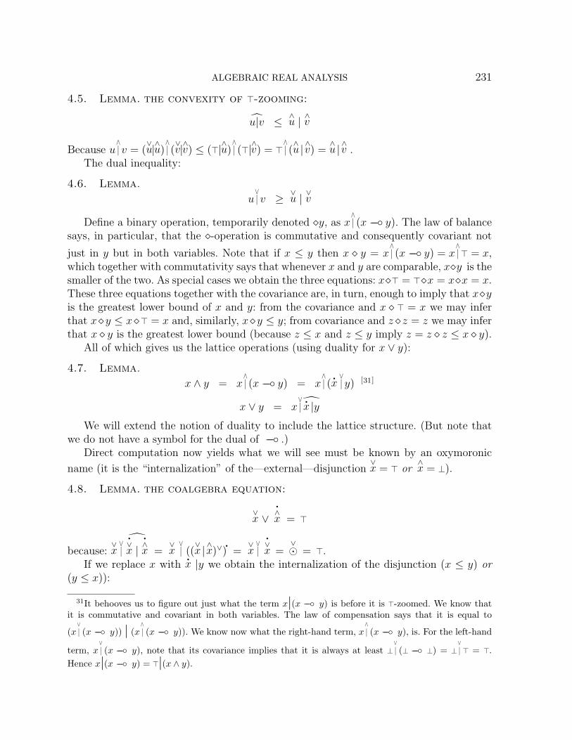
4.5. Lemma. the convexity of >-zooming:

u|v ≤ ∧u | ∧v

Because u |∧v = (

∨u|∧u) |

∧(∨v|∧v) ≤ (>|∧u) |

∧(>|∧v) = > |

∧(∧u | ∧v) =

∧u | ∧v .

The dual inequality:

4.6. Lemma.

u |∨v ≥ ∨

u | ∨v

Define a binary operation, temporarily denoted y, as x |∧(x −− y). The law of balance

says, in particular, that the -operation is commutative and consequently covariant not

just in y but in both variables. Note that if x ≤ y then x y = x |∧(x −− y) = x |

∧> = x,

which together with commutativity says that whenever x and y are comparable, xy is thesmaller of the two. As special cases we obtain the three equations: x> = >x = xx = x.These three equations together with the covariance are, in turn, enough to imply that xyis the greatest lower bound of x and y: from the covariance and x > = x we may inferthat xy ≤ x> = x and, similarly, xy ≤ y; from covariance and z z = z we may inferthat x y is the greatest lower bound (because z ≤ x and z ≤ y imply z = z z ≤ x y).

All of which gives us the lattice operations (using duality for x ∨ y):

4.7. Lemma.

x ∧ y = x |∧(x −− y) = x |

∧(.x |∨y) [31]

x ∨ y = x |∨ .x |y

We will extend the notion of duality to include the lattice structure. (But note thatwe do not have a symbol for the dual of −− .)

Direct computation now yields what we will see must be known by an oxymoronic

name (it is the “internalization” of the—external—disjunction∨x = > or

∧x = ⊥).

4.8. Lemma. the coalgebra equation:

∨x ∨

.∧x = >

because:∨x |∨

.∨x |

.∧x =

∨x |

∨((∨x | ∧x)∨)

.=

∨x |∨

.∨x =

∨ = >.

If we replace x with.x |y we obtain the internalization of the disjunction (x ≤ y) or

(y ≤ x)):

31It behooves us to figure out just what the term x|(x −− y) is before it is >-zoomed. We know thatit is commutative and covariant in both variables. The law of compensation says that it is equal to

(x |∨

(x −− y)) | (x |∧

(x −− y)). We know now what the right-hand term, x |∧

(x −− y), is. For the left-hand

term, x |∨

(x −− y), note that its covariance implies that it is always at least ⊥ |∨

(⊥ −− ⊥) = ⊥ |∨> = >.

Hence x|(x −− y) = >|(x ∧ y).

232 PETER FREYD

4.9. Lemma. the equation of linearity:

(x −− y) ∨ (y −− x) = > [32]

Indeed it says that what logicians call the disjunction property (the principle thata disjunction equals > only if one of the terms equals >) is equivalent with linearity.The following are equivalent for scales: linearity, the disjunction property, the coalgebracondition.

We will need:

4.10. Lemma. the adjointness lemma:

u ≤ v −− w iff u |∧v ≤ w

Because if u ≤ v −− w then v|u ≤ v|(v −− w) = w|(w −− v) ≤ w|> and we may >-zoom

the two ends to obtain u |∧v ≤ w. And if u |

∧v ≤ w then v −− u|v ≤ v −− w. But v −− u|v =

.v |∨u|v = u∨ .

v hence we have u ≤ u∨ .v ≤ v −− w. [33]

We close this section with a few interval isomorphisms. For any b < t the interval[b, t| is order-isomorphic with an interval whose top end-point is >, to wit, the interval

[t −− b,>]. The isomorphism is t −− (−). Its inverse is t |∧(−). (The fact that the composi-

tion t |∧(t −− x) = x for all x ∈ [b, t] is just the fact that t |

∧(t −− x) = t ∧ x. The fact that

the composition t −− (t |∧x) = x for all x ∈ [t −− b,>] is just the fact that

.t |∨(t |

∧x) =

.t∨x

and the fact that x ≥ (t −− b) implies x ≥ (t −− b) ≥ (t −− ⊥) =.t.) These are not just

order-isomorphisms. With the forthcoming linear representation theorem (Section 8) itwill be easy to prove that they preserve midpointing and when—in Section 6—we notethat all closed intervals have intrinsic scale structures it will be easy to see that they arescale isomorphisms.[34]

32The coalgebra equation is obtainable, in turn, from the equation of linearity by replacing y with.x.

33Using the linear representation theorem below one can show the rather surprising fact that the binary

operation |∧

is associative. Any poset may be viewed as a category and this associativity together with

the adjointness lemma allows us to view a scale as a “symmetric monoidal closed category” with |∧

asthe monoidal product and −− as the closed structure. The monoidal unit is >. A scale is, in fact, a“?-autonomous category”: ⊥ is its “dualizing object.”

A straightforward verification of the associativity of |∧

on a linear scale entails a lot of case analysis.Perhaps it is best to use the equational completion that will be proved. It then suffices to verify it onjust one non-trivial example. The easiest we have found is to take the unit interval—not the standard

interval—and to verify the dual equation, the associativity of |∨

. On the unit interval x |∨y is addition

truncated at 1, quite easily seen to be associative.34The construction of the dilatation operator can be motivated by this material. For any a, the function

(a|>) −− (−) sends the image of a|− to the interval [,>], quite enough to suggest that (a|>) −− (a|−)is the same as >|−, hence (using the unital law) that (a|>)−−(a|x) = x. The function (a|>)−−(−) is a/−.


5. Diversion: Lukasiewicz vs. Girard

On the unit interval the formula for −− has a prior history as the Lukasiewicz notion ofmany-valued logical implication. A traditional interpretation of Φ ≤ Ψ is “Ψ is at least aslikely as Φ.” Then Φ −−Ψ becomes the “likelihood of Ψ being at least as likely as Φ.” [35]

The unit interval when viewed as a ?-autonomous category (resulting from its scale-algebra structure) reveals Lukasiewicz inference as a special case of Girard’s linear logic.

We will write |∧

as ⊗ and its “de Morgan dual” |∨

as

&

(“par”). (The midpoint operationis an example of a “seq” operation—it lies between ⊗ and

&

.)If we interpret the truth-values as frequencies (or probabilities) we can not infer, of

course, the frequency of a conjunction from the individual frequencies. But we can infer therange of possible frequencies. If Φ and Ψ are the individual frequencies then the maximumpossible frequency for their disjunction occurs when they are maximally exclusive: if theirfrequencies add to 1 or less and if they never occur together then the maximal possiblefrequency of the disjunction is their sum; if their frequencies add to more than 1 thenthe maximal possible frequency of the disjunction is, of course, 1. That is, the maximumpossible frequency for their disjunction is Φ

&

Ψ. The minimal possible frequency for theirconjunction likewise occurs when they are maximally exclusive and similar considerationyields Φ⊗Ψ. This works best if we understand that separate observations are made, onefor Φ and one for Ψ (hence Φ⊗Φ is the minimal possible frequency that Φ occurs in bothobservations, Φ

&Φ the maximal possible frequency that Φ occurs in at least one of the

two observations).The “additive” connectives, likewise, have such an interpretation. The minimal pos-

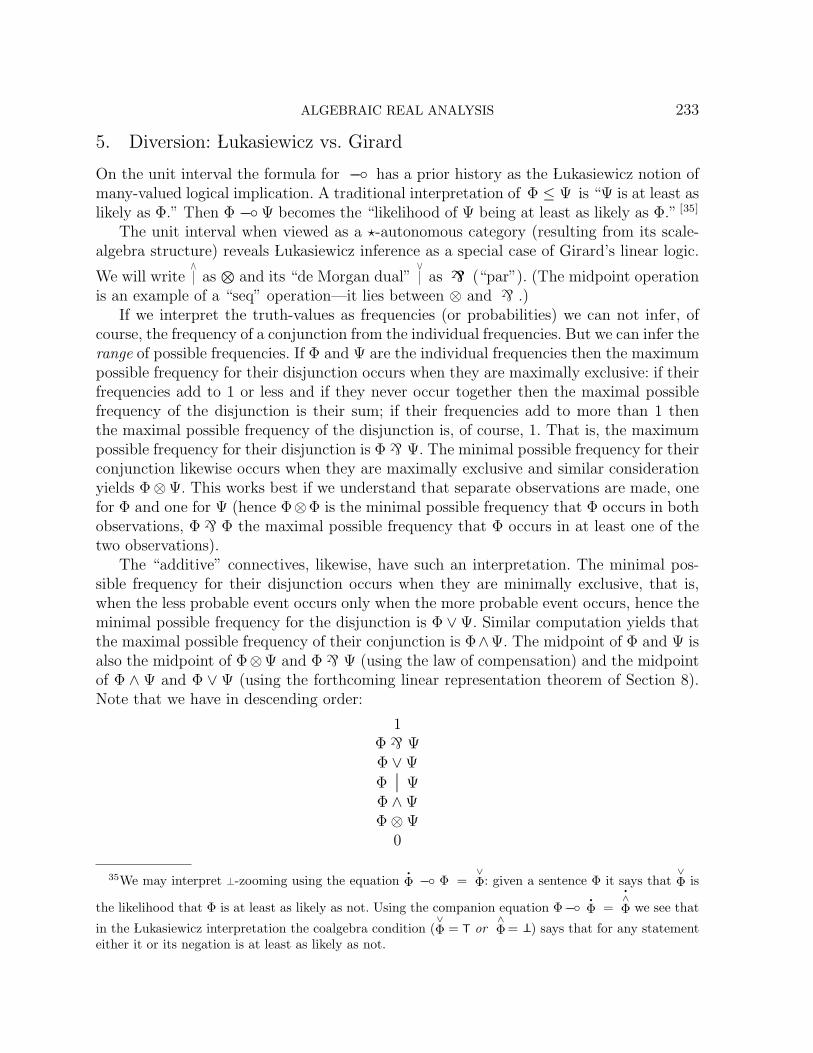
sible frequency for their disjunction occurs when they are minimally exclusive, that is,when the less probable event occurs only when the more probable event occurs, hence theminimal possible frequency for the disjunction is Φ ∨Ψ. Similar computation yields thatthe maximal possible frequency of their conjunction is Φ∧Ψ. The midpoint of Φ and Ψ isalso the midpoint of Φ⊗Ψ and Φ

&

Ψ (using the law of compensation) and the midpointof Φ ∧ Ψ and Φ ∨ Ψ (using the forthcoming linear representation theorem of Section 8).Note that we have in descending order:

1Φ

&

ΨΦ ∨Ψ

Φ | ΨΦ ∧ΨΦ⊗Ψ

0

35We may interpret ⊥-zooming using the equation.Φ −− Φ =

∨Φ: given a sentence Φ it says that

∨Φ is

the likelihood that Φ is at least as likely as not. Using the companion equation Φ−−.Φ =

.∧Φ we see that

in the Lukasiewicz interpretation the coalgebra condition (∨Φ = T or

∧Φ =

T

) says that for any statementeither it or its negation is at least as likely as not.

234 PETER FREYD

Φ −−Ψ = 1 means that it is possible (just knowing the frequencies of Φ and Ψ) thatwhenever Φ occurs Ψ will occur. In general Φ −−Ψ gives the maximal possible probabilitythat a single pair of observations will fail to falsify the hypothesis “if Φ then Ψ.” Theadjointness lemma, Φ ≤ Ψ −− Λ ⇔ Φ⊗Ψ ≤ Λ, then says that Φ is possibly less frequentthan Ψ appearing to imply Λ iff the frequency of the conjunction of Φ and Ψ is possiblyless than the frequency of Λ. [36] We constructed the meet operation as Φ ⊗ (Φ −−Ψ).That is, the maximal possible frequency for the conjuction of two events is equal to theminimal possible frequency of the conjunction of another pair of events, the first of whichremains the same and the second is the maximal possible frequency of failing to refutethe hypothesis that the first implies the second. (Surely someone previously must haveobserved this.)

When the coalgebra condition is interpreted we obtain the interval rule:

Φ

&

Ψ = 1 or Φ⊗Ψ = 0

(Either it is possible for one to succeed or it is possible that both fail.) Alternatively we

may replace Φ with.Φ so that the coalgebra condition becomes

Φ ≤ Ψ or Ψ ≤ Φ

delivering a theory of linear linear logic.[37]

Missing above are Girard’s modal unary operations, of-course and why-not, which hedenoted with a ! and a ?. [38] In Section 19, below, on “chromatic scales” we introducethe (discontinuous) “support” operations on scales. Using chromatic-scale notation onemay argue that !Φ = Φ and ?Φ = Φ.

6. Diversion: The Final Interval Coalgebra is a Scale

The final interval coalgebra, I, comes equipped, of course, with the two constants > and

⊥, and the two zooming operations∧x and

∨x. We may define

.x via the unique coalgebra

map.I→ I where

.I is the coalgebra obtained by swapping the two constants and the two

zooming operations. The order on I is definable via the observation that x < y iff thereis a sequence of zooming operations (∧, ∨) that carries x to ⊥ and y to >.

There is, indeed, a useful interval coalgebra structure on I × I so that its uniquecoalgebra map to I is the midpoint operation,[39] but, alas, this coalgebra structure on

36This would not, of course, be heard as an acceptable sentence in ordinary language. But few transla-tions from the mathematical notation to ordinary language yield acceptable sentences—else who wouldneed the math?

37That which is linear2 is planar.38Hollow men pronounce these as bang and whimper.39The word “useful” is important here. Given any functor T with a final coalgebra F → TF then for

any retraction Fx→ A

y→ F = 1F there is a coalgebra structure on A that makes y a coalgebra map, to

wit, Ay→ F → TF

Tx→ TA.


I×I requires the midpoint operation for the construction of its two zooming operations:

〈u, v〉 is sent by >-zooming to 〈 ∨u |∧ ∧v ,

∧u |∧ ∨v 〉 and by ⊥-zooming to 〈 ∨u |

∨ ∧v ,

∧u |∨ ∨v 〉. [40]

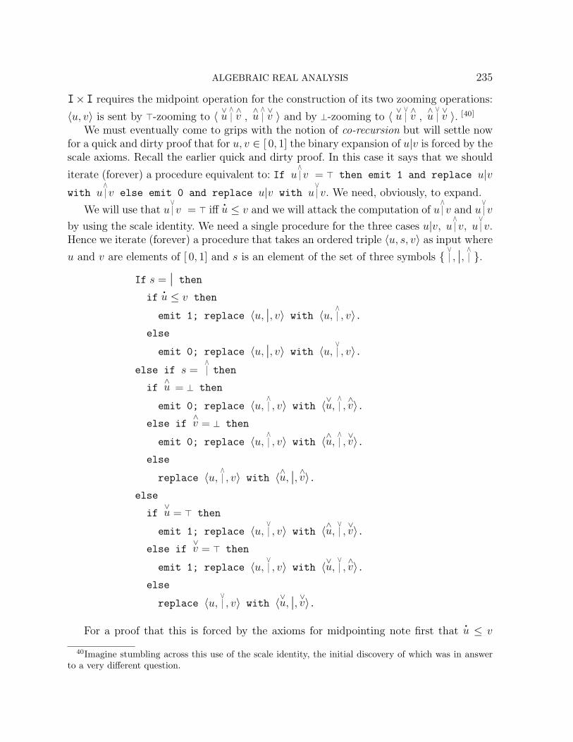
We must eventually come to grips with the notion of co-recursion but will settle nowfor a quick and dirty proof that for u, v ∈ [ 0, 1] the binary expansion of u|v is forced by thescale axioms. Recall the earlier quick and dirty proof. In this case it says that we should

iterate (forever) a procedure equivalent to: If u |∧v = > then emit 1 and replace u|v

with u |∧v else emit 0 and replace u|v with u |

∨v. We need, obviously, to expand.

We will use that u |∨v = > iff

.u ≤ v and we will attack the computation of u |

∧v and u |

∨v

by using the scale identity. We need a single procedure for the three cases u|v, u |∧v, u |

∨v.

Hence we iterate (forever) a procedure that takes an ordered triple 〈u, s, v〉 as input where

u and v are elements of [ 0, 1] and s is an element of the set of three symbols |∨, |, |∧ .

If s = | then

if.u ≤ v then

emit 1; replace 〈u, |, v〉 with 〈u, |∧, v〉.

else

emit 0; replace 〈u, |, v〉 with 〈u, |∨, v〉.

else if s = |∧then

if∧u = ⊥ then

emit 0; replace 〈u, |∧, v〉 with 〈∨u, |

∧,∧v〉.

else if∧v = ⊥ then

emit 0; replace 〈u, |∧, v〉 with 〈∧u, |

∧,∨v〉.

else

replace 〈u, |∧, v〉 with 〈∧u, |, ∧v〉.

else

if∨u = > then

emit 1; replace 〈u, |∨, v〉 with 〈∧u, |

∨,∨v〉.

else if∨v = > then

emit 1; replace 〈u, |∨, v〉 with 〈∨u, |

∨,∧v〉.

else

replace 〈u, |∨, v〉 with 〈∨u, |, ∨v〉.

For a proof that this is forced by the axioms for midpointing note first that.u ≤ v

40Imagine stumbling across this use of the scale identity, the initial discovery of which was in answerto a very different question.

236 PETER FREYD

implies ≤ u|v, hence u |∨v = > which means that the first digit is 1 and the remaining

digits are determined by u |∧v. For u |

∧v we use the scale identity:

u |∧v = (

∨u |

∧ ∧v) | (

∧u |

∧ ∨v)

When∧u = ⊥ this becomes:

u |∧v = (

∨u |

∧ ∧v) | (⊥ |

∧ ∨v) = (

∨u |

∧ ∧v)|⊥

hence, by the absorbing law, (u |∧v)∧ = ⊥ which means that the first digit is 0 and the

remaining digits are determined by (u |∧v)∨ = ((

∨u |

∧ ∧v) | ⊥)∨ which by the unital law is

∨u |

∧ ∧v. A similar argument holds for the case

∧v = ⊥. If neither

∧u nor

∧v are ⊥ we have

∨u =

∨v = > and the scale identity and unital law yield

u |∧v = (> |

∧ ∧v) | (

∧u |

∧>) =

∧v | ∧u

which returns us to the case s = |. The dual argument holds for the case s = |∨.

7. Congruences, or: >–Faces

One of our first aims is to prove that every scale can be embedded in a product of linearscales. Put another way: we wish to find, on any scale, a lot of quotient structures thatare linearly ordered. And for that we must get an understanding of quotient structures.

As for any equational theory, the quotient structures of a particular algebra corre-spond to the “congruences” on that structure, that is, the equivalence relations that arecompatible with the operators that define the structure. For some well-endowed theoriesthe congruences correspond, in turn, to certain subsets. Such is the case for scales.[41]

Given a congruence ≡ define its kernel, denoted ker(≡), to be the set of elementscongruent to >. Clearly, ≡ can be recovered from ker(≡) (because x ≡ y iff both x −− yand y −− x are in ker(≡)). We need to characterize the subsets that appear as kernels.

Borrowing again from convex-set terminology, we say that a subset is a “face” ifit is not just closed under midpointing but has the property that it includes any twoelements whenever it includes their midpoint. (Saying that an element is an extremepoint, therefore, is the same as saying that it forms a one-element face.) We will beinterested particularly in those faces that include >. Thus we define a subset, F , to be aT-face, “top-face,” if:

> ∈ Fx|y ∈ F iff x ∈ F and y ∈ F

41Almost all well-endowed theories in nature contain the theory of groups. Two exceptions (besidesscales): the theory of Heyting algebras and (its generalization) the theory of division allegories.


Because inverse homomorphic images of faces are faces and because > is a face itis clear that ker(≡) is a >-face for any congruence. We need to show that all >-faces soarise.

Given a >-face, F , define x y (mod F) to mean x −− y ∈ F and definex ≡ y (mod F) as the “symmetric part” of , that is, x ≡ y iff x y and y x.It is routine that x ≡ > iff x ∈ F .

Clearly ≡ is reflexive (because x −− x = >) and it is symmetric by fiat. Transitivityrequires a little more. First note that a >-face is an updeal, that is, x ∈ F and x ≤ yimply y ∈ F (immediate from the law of balance). Second, in the dual of the convexity

of >-zooming,∨u | ∨v ≤ u |

∨v, replace u with

.w |x and v with

.x |y to obtain:

(w −− x) | (x −− y) ≤ >|(w −− y) [42]

because (w −− x)|(x −− y) = (.w |

∨x)|( .x |

∨y) ≤ (

.w |x) |

∨(.x |y) = (

.x |x) |

∨(.w |y) = |

∨(.w |y) =

>|( .w |

∨y) = >|(w −− y). Hence if w x and x y then (w −− x)|(x −− y) ∈ F forcing

>|(w −− y) ∈ F and, finally, (w −− y) ∈ F .Thus ≡ is an equivalence relation. It is a congruence with respect to dotting because

w −− x =.x −− .

w, hence.w .

x iff x w. In the verification that y| is covariant weused the equation (y|w) −− (y|x) = >|(w −− x) which quite suffices to show that w xiff y|w y|x and consequently that ≡ is a congruence with respect to midpointing.Finally, to see that ≡ is a congruence with respect to zooming it suffices to show that

w x implies∧w ∧

x. We may as well show that it implies∨w ∨

x at the same time. The

scale identity, in the form w −− x = (∧w −− ∧

x) | (∨w −− ∨

x) does just that.Given an element, a, in a scale we will need to see how to construct ((a )) the

principal T-face it generates, that is, the smallest >-face containing a.

7.1. Lemma. The principal >-face, ((a )), is the set of all x such that a ≤ (>|)nx for alllarge n.

((>|)n is the nth iterate of the contraction at >.) Clearly this set includes > andis closed under midpointing; for the other direction, suppose it includes x|y; then froma ≤ (>|)n(x|y) we may infer a ≤ (>|)n(x|y) ≤ (>|)n(>|y) = (>|)n+1y for sufficiently largen and y is clearly in the set. For the other direction note that in any quotient where abecomes > the inequality a ≤ (>|)nx clearly forces (>|)nx to become >, after which n

42If both sides of this inequality are >-zoomed we obtain

(w −− x) |∧

(x −− y) ≤ (w −− y).

When this inequality is viewed as a map in a monoidal closed category:

(w −− x)⊗ (x −− y) → (w −− y)

its name is the “composition map.”

238 PETER FREYD

applications of >-zooming will force x itself to be >. That is, if a ≤ (>|)nx for any n, thenx must be in any >-face that contains a.

8. The Linear Representation Theorem

We wish to prove:

8.1. Theorem. Every scale can be embedded in a product of linear scales.

An algebra (for any equational theory) is said to be sub-directly irreducible, orSDI for short, if whenever it is embedded into a product of algebras one of the coordinatemaps is itself an embedding. Every algebra (for any equational theory) is embedded inthe product of all of its sdi quotients (we will repeat the proof for this case). But first:

8.2. Lemma. If a scale is an sdi then it is linearly ordered.

A homomorphism of scales is an embedding iff its kernel is trivial. A scale is an sdiiff the map into the product of all of its proper quotient scales fails to be an embedding.Hence it is an sdi iff the intersection of all non-trivial >-faces is non-trivial. Let s < > bean element in that minimal non-trivial >-face. Then for every element a < >, its principal>-face, ((a )), must contain s. Thus an sdi scale has an element s < > such that for alla < > it is the case that a < (>|)ns for almost all n. (This may be rephrased: a scale isan sdi iff there is a sequence of the form (>|)nsn cofinal among elements below >.) Ifx and y are both below > then clearly x ∨ y < (>|)ns almost all n, in particular x ∨ y isbelow top. That is, sdi scales satisfy the disjunction property which, as has already beenobserved, implies linearity via the equation of linearity, (x −− y) ∨ (y −− x) = >.

The fact that all scales can be embedded in a product of linear scales is now easilyobtainable: for each element s < > use the axiom of choice to obtain a >-face, Fs, maximalamong >-faces that exclude s; it is routine that in the corresponding quotient scale theelement in the image of s becomes equal to > in every proper quotient thereof hence is, asjust argued, linearly ordered. The intersection of all the >-faces of the form Fs is clearlytrivial. (Note that the structure of this proof of the linear representation theorem is forced:if the result is true then necessarily every sdi is linear and the theorem is equivalent tosdis being linear.)

An immediate corollary:

8.3. Corollary. Every equation, indeed every universal Horn sentence, true for alllinear scales is true for all scales.

It should be noted that the axiom of choice is avoidable for purposes of this corollary.Given a Horn sentence,

(s1 = t1) & · · ·& (sn = tn) ⇒ (u = v)

suppose there were a counterexample in some scale, A. The elements used for the coun-terexample generate a countable subscale, A′. The term (u −− v) ∧ (v −− u) evaluates to

an element b < >. We can construct a >-face, F , in A′ maximal among those that excludeb without using choice since A′ is countable. The image of the counterexample in thelinear scale A′/F remains a counterexample.

When working with a linearly ordered set it is completely trivial that covariant func-tions automatically distribute with the lattice operations. Hence for all scales we have:

x|(y ∧ z) = (x|y) ∧ (x|z)

x|(y ∨ z) = (x|y) ∨ (x|z)

x ∧ z =∧x ∧

∧y

x ∨ z =∧x ∨

∧y

(x ∧ z)∨ =∨x ∧

∨y

(x ∨ z)∨ =∨x ∨

∨y

x ∧ (y ∨ z) = (x ∧ y) ∨ (x ∧ z)x ∨ (y ∧ z) = (x ∨ y) ∧ (x ∨ z)

(The last two equations—the definition of distributive lattices—are, of course, equiv-alent in any lattice.)

It is easy to check that if f is any binary operation on a linear scale satisfying the“dilatation equation,” f〈a, a|x〉 = x, and if, further, for any fixed a it is covariant in x,then f〈a, x〉 = a/ x, hence dilatations are self-dual.[43]

Using the linear representation theorem we obtain a proof for a lemma that we willneed later:

8.4. Lemma. The image of the central contraction, |, is the sub-interval [⊥|,|>].

We need to show that if |⊥ ≤ x ≤ |> then we can solve for x = |y. We removethe existential to obtain a Horn sentence by setting y = / x. Thus we need to show thatin any linear scale |⊥ ≤ x ≤ |> implies x = |(/ x). Linearity allows us to reduce tothe two cases x ≤ and ≤ x. Symmetry allows us to concentrate on the case ≤ x,

hence we can assume x =∨x | ∧x = >| ∧x. From x ≤ |> we infer that

∧x ≤ |> = hence

that∧x =

∨∧x |

∧∧x =

∨∧x |⊥ which combines to give x = >|(⊥|

∨∧x) = (>|⊥)|(>|

∨∧x) = |(>|

∨∧x).

(So y = >|∨∧x.) It is routine now that |(/ x) = x. [44]

43As promised, we now have (((.a |⊥)|x) ) = (((

.a |>)|x) ) . There are two other corollaries of interest.

First, any dilatation is definable using just central dilatation: a/ x = / (/ ((.a |)|x)) because the one

appearance of x is in a covariant position and/(/((.a |)|(a|x))) = /(/((

.a |a)|(|x))) = /(|x) = x.

Second, central dilatation is definable using (twice) any one dilatation: / x = a/ (a/ ((|a)| .x)).because

the one appearance of x is in a covariant position and a/ (a/ ((|a)|(|x).)).= a/ (a/ ((|a)|(| .x)))

.=

a/ (a/ (|(a| .x))).= a/ (a/ ((a| .a |(a| .x))))

.= a/ (a/ (a|( .a | .x)))

.= a/ (

.a | .x)

.= a/ (a|x) = x. Hence any one

dilatation can be used to construct any other dilatation.44Let x denote the central dilatation /x. We could take x as primitive and define

∧x as (⊥|)|x. There

240 PETER FREYD

The fact that >-zooming distributes with meet has an important application: thelattice of congruences is distributive. Recall, first, that in any lattice a set is called a “filter”if it is hereditary upwards and closed under finite meets.[45] By a zoom-invariant filterwe mean a filter closed under the zooming operations. Since ⊥-zooming is inflationary afilter is zoom-invariant iff it is closed under >-zooming. An important lemma:

8.5. Lemma. A subset of a scale is a >-face iff it is a zoom-invariant filter.

Because: suppose that F is a filter invariant with respect to zooming; from x ∧ y =(x ∧ y) | (x ∧ y) ≤ x|y we know that F is closed under midpointing; that it is a face

follows immediately from x|y ≤ x|> = x.The other direction is an immediate consequence of the facts that zoom-invariant

filters are preserved under inverse images of homomorphisms and that any >-face is theinverse image of a one-element zoom-invariant filter, to wit, >. (It is not hard to give adirect proof: we have already noted that the law of balance says that if x is an element of

a >-face, F , and if x ≤ y then y ∈ F ; the law of compensation easily implies that∧x ∈ F ;

and if x and y are both in F we finish with x|y ≤ x|> = x and similarly x|y ≤ y hence

x|y ≤ x ∧ y.)

8.6. Theorem. The congruence lattice of any scale is a spatial locale

The pre-ordained name for the space in question is the spectrum of S, denotedSpec(S).

First, the lattice of filters in any distributive lattice is itself a distributive latticeand the argument continues to work when we replace “filter” with “zoom-invariant fil-

is something to be said for this choice. x (unlike∧x and

∨x) appears as an innate operation on almost any

graphic calculator. At first glance it looks like we could reduce by one the number of axioms. We wouldtake the single |x = x and use the previous footnote to obtain the two unital laws.

The important reason for not using this definition is that the origin of the notion of scales would bebelied. But there is another: even when the scale identity is translated into this language the equationsare not complete. They do not fix the primitive operation, x. For a separating example take any scale anddefine x as the standard central dilatation with one exception: redefine > any way one chooses. Thus—besides the translation of the scale identity—a further equation is needed to fix the primitive x operationas defined from

∧x. (Without such, note that there is no way of proving that the primitive operation x

is covariant, hence no way of showing that >-faces arise from congruences and no way of obtaining thelinear representation theorem.)

One could redo the notion of minor scale using x as the primitive. After the constant law add thethree equations |x = x, >|(>|x) = >, and ⊥|(⊥|x) = ⊥. The proofs that the elements named by thetyped terms are closed under dotting and midpointing remains unchanged. That they are closed underx one need only verify > = >|(>|>) = >, ⊥ = ⊥|(⊥|⊥) = ⊥, >|(⊥|x) = (>|⊥)|(>|x) = >|x, and, similarly,⊥|(>|x) = ⊥|x. The previous argument that the theory has a unique consistent equational completion stillholds.

45It’s worth noting—in the context of scales— an alternative definition: F is a filter if> ∈ F

x ∧ y ∈ F iff x ∈ F and y ∈ F


ter.” The main observation (for both proofs) is that the join of filters F and G is the set x ∧ y : x ∈ F, y ∈ G . (It is clearly closed under meet and >-zooming. Ifx ∧ y ≤ z then, using distributivity of the lattice, z = (x ∨ z) ∧ (y ∨ z) where, ofcourse, x ∨ z ∈ F and y ∨ z ∈ G.)

To see that (F ∨ G) ∩ H ⊆ (F ∩H) ∨ (G ∩ H) (the reverse containment holds in anylattice) we note that an arbitrary element in the left-hand side is of the form x∧ y wherex ∈ F , y ∈ G and x ∧ y ∈ H. But the last condition implies that both x and y are in H.Hence, x ∈ F ∩H and y ∈ G ∩H, thus x ∧ y ∈ (F ∩H) ∨ (G ∩ H).

Distributivity, recall, is quite enough to establish that a lattice of congruences is alocale, that is, finite meets distribute with arbitrary joins. It is always a spatial locale:the points are the “prime” congruences, that is, those that are not the intersection of twolarger congruences. Translated to filters: F is a point if it has the property that wheneverx ∨ y ∈ F it is the case that either x ∈ F or y ∈ F . Put another way, of course, thepoints of Spec(S) are the linearly ordered quotients of S. We will show that Spec(S) iscompact normal (but not always Hausdorff). We obtain—just as in the ancestral subjectof spectra for associative algebras—a representation of an arbitrary scale as the scale ofglobal sections of a sheaf of linear scales.[46]

We pause to obtain a “pushout lemma” for scales:

8.7. Lemma. Let A → B be monic and A → C a quotient map. Then in the pushout

A → B↓ ↓C → D

the map C → D is monic (and, as in any category of algebras, B → D is a quotientmap).

Because, if we view A as a subscale of B and take F = ker(A → C) then we obtaina >-face of B, to wit, F ⇑ = b ∈ B : ∃a∈A a ≤ b . It is easy to check that F ⇑ iszoom-invariant and that A∩F ⇑ = F . Define D = B/F ⇑. The map A → B → D has thesame kernel as A → C and we obtain an embedding C → D. It is easily checked to yielda pushout diagram.[47]

46Recall that the space of points of a spatial locale is always “sober” (most easily defined as a spacemaximal among T0 spaces with the given locale of open sets). There is often a minimal space, one with thefewest points (the pre-ordained name for this condition is “spaced-out”). For any distributive congruencelattice this minimal space does exist: its elements are the congruences of the sdi quotients. (Could thisconnection between universal algebra and Stone theory be new?)

47This pushout lemma fails in most equational theories. In the category of groups let A → B be theinclusion map of a subgroup and A → C be an epi whose kernel is A′. Then the kernel of C → D isthe image in C of the intersection of A with the normal closure of A′ in B. If one takes B to be thealternating group of order 12, A the unique subgroup of order 4 (the original Klein group), and A′ oneof its 2-element subgroups, then the kernel of B → D is all of A, and C → D is the trivial map from the2-element cyclic group to the 3-element cyclic group. A more dramatic example is to enlarge B to thealternating group or order 60; D then collapses to a 1-element group.

242 PETER FREYD

9. Lipschitz Extensions and I-Scales

Given an equational theory T, we may say that an extension T ′ is “co-congruent” ifcongruences for the operations in T remain congruences for all the operations in T ′. Ifall new operations are constant then the extension is automatically co-congruent (e.g.the theory of monoids is a co-congruent extension of the theory of semigroups). A moreinteresting example is the next step: a monoid congruence is automatically a congruencewith respect to the entire group structure (because x ≡ y implies x−1 = x−1yy−1 ≡x−1xy−1 = y−1). [48]

An extension of the theory of scales is co-congruent iff the equivalence relation deter-mined by any >-face respects the new operations that appear in the extended theory. Wewill use x −− y to denote (x −− y)∧ (y −− x). A new unary operator f is co-congruentif every >-face F that contains the element x −− y also contains the element fx −− fy.If we take F to be the principal >-face ((x −− y )) then for co-congruence to hold we musthave, for some integer n,

x −− y ≤ (>|)n(fx −− fy)

When interpreted on the standard interval this becomes the assertion that f is Lipschitzcontinuous (with Lipschitz constant ≤ 2n):

|fx− fy| ≤ 2n|x− y| [49]

If we move to the free algebra on two generators for the extended theory we see thatco-congruence requires the existence of an n that works in all models. The argument for

48There are several similar examples that involve a unary involutory operation that delivers somethinglike an inverse. A lattice-congruence on a Boolean algebra is automatically a congruence for negation: ifx ≡ y then ¬x = ¬x ∧ (y ∨ ¬y) ≡ ¬x ∧ (x ∨ ¬y) = ¬x ∧ ¬y = (¬x ∨ y) ∧ ¬y ≡ (¬x ∨ x) ∧ ¬y = ¬y. Aring-congruence on a von Neumann strongly regular ring is automatically a congruence for the “pseudo-inverse” (to wit, the unary operation that satisfies x2x∗ = x = x∗∗): if x ≡ y then (using that xx∗ = x∗xis a consequence of the axioms) x∗ = x∗2x ≡ x∗2y = x∗2y2y∗ = x∗2y(y2y∗)y∗ = x∗2y3y∗2 ≡ x∗2x3y∗2 =x∗(x∗x2)xy∗2 = x∗x2y∗2 = xy∗2 ≡ yy∗2 = y∗.

A congruence on a scale with respect to midpointing and the two zoom operations is automati-cally a congruence for dotting: if u ≡ v then

.u = (>| .

u) = ((⊥|(>| .u)) ) = (((⊥|>)|(⊥| .

u)) ) =

(((.u |u)|(⊥| .u)) ) = (((

.u |⊥)|(u| .u)) ) = (((

.u |⊥)|(v| .v)) ) ≡ (((

.u |⊥)|(u| .v)) ) = (((

.u |u)|(⊥| .v)) ) =

(((⊥|>)|(⊥|.v)) ) = ((⊥|(>|.v)) ) = (>|.v) =.v.

But these three examples are misleading. In each case the new operation is unique—when it exists—given the old structure. As we will see such is not the case for all the co-congruent extensions of the theoryof scales. Nor is the uniqueness sufficient. A meet semi-lattice has at most one lattice structure but noticethat on the four-element non-linear lattice the equivalence relation that smashes the three elementsbelow the top to a single point is a meet- but not a lattice-congruence. A lattice has at most one Heyting-algebra structure but the only non-trivial variety of Heyting algebras in which lattice-congruences areautomatically Heyting congruences is the variety of Boolean algebras: any non-Boolean Heyting algebracontains a three-element subalgebra and the equivalence relation on the three-element Heyting algebrathat smashes the bottom two elements to a point is a lattice- but not a Heyting-algebra congruence.

49On the unit interval x•−− y (the dotting operation applied to x −− y) is |x−y|. The dual inequality

of x −− y ≤ (>|)n(fx −− fy) is (⊥|)n(fx•−− fy) ≤ x

•−− y.


unary operations easily extends to arbitrary arities. Hence for extensions of the theory ofscales we will use the phrase Lipschitz extension instead of “co-congruent extension.”

The first application is that Lipschitz extensions of the theory of scales all enjoy thelinear representation theorem. (More important will be the consequence of the section tocome: every consistent Lipschitz extension has an interpretation on the standard intervalI.)

If M is a monoid, we understand an M-scale to be a scale on which M acts. Wewill not require that the M -actions be endomorphisms of the entire scale structure oranything else in particular. In all the cases to be discussed, however, the actions willpreserve midpointing.

We will be particularly interested in two cases: when M = I and when M is thesubmonoid of rationals in the standard interval. The theory of I-scales is obtained byadding a unary operator for every r ∈ I whose value at x is denoted rx and that satisfiesthe equations:

r =

r(x|y) = rx|ry

and for all q ∈ I with q ≥ r the equation [50]

q ≥ r>

and if q ≤ rq ≤ r>

There is obviously a unique interpretation of these operations on the standard intervalI. [51] The theory is not as it stands Lipschitz.[52] So we add the condition

x −− y ≤ rx −− ry

9.1. Lemma. Any scale is embedded in its I-scale reflection.

Because given a scale S consider the equational theory obtained by adding to thetheory of scales a constant for each element of S and adding as equations all the variable-free equations in these constants that hold for S. Now add the I-scale structure. As forits consistency we use the “compactness argument”: every finite set of equations in thisextended theory has a model (for each relevant r ∈ I we can find q ∈ I that will satisfythe finite number of equations that involve r) and such suffices for consistency.

It is a consequence of the results in the next section that this newly constructed I-scalehas a quotient isomorphic to I with its unique action.

50Bear in mind that in the presence of a lattice operation any inequality is equational: x ≤ y isequivalent with x = x ∧ y.

51It was discussed above in the last footnote of Section 6.52Order the polynomial ring R[ε] by stipulating P (ε) ≥ 0 iff P (1/n) ≥ 0 for all sufficiently large n.

Its standard interval is a scale and the map that sends P (ε) to P (2ε) is a scale-automorphism thereon,hence easily satisfies the equations (with r = 1). It is not Lipschitz.

244 PETER FREYD

Every scale may be viewed as an I-scale: we may define qx for q ∈ I and x in anarbitrary scale using the inductive scheme introduced in the construction of I: for type-0terms take >x = x and ⊥x =

.x and for all higher-typed term, q, take (>|q)x = x|(qx) and

(⊥|q)x =.x |(qx). [53]

10. Simple Scales

10.1. Theorem. A scale is simple iff the sequence ⊥,>|⊥,>|(>|⊥), . . . , (>|)n⊥, . . . iscofinal among all elements below >.

The cofinality clearly implies simplicity: if F is a non-trivial >-face then necessarilythere exists x ∈ F , x 6= > and the cofinality says that (>|)n(⊥) ∈ F for some n, hencethat ⊥ ∈ F , which means—of course—that F is entire. Conversely, a simple algebra isnecessarily an sdi, hence necessarily linear; but we have much more. We may take theelement s used above in the characterization of sdis to be the element ⊥. Then, since ⊥is included in every non-trivial >-face (because in a simple scale the entire set is the onlynon-trivial >-face) we know that the sequence (>|)n(⊥) is cofinal among all elementsbelow >.

A scale satisfying this condition is called, of course, Archimedean.[54]

10.2. Lemma. A scale is simple iff between any two elements there is a constant (thatis, an element from the initial subscale).

One direction is immediate: if between > and any x < > there is some constant, thenthere must be one of the form (>|)n(⊥). The other direction requires a little work. Given

53The set of operations that preserve midpointing and form a closed midpoint algebra and we cansee this action of I on arbitrary scales as a consequence of the fact that I is the initial closed midpointalgebra.

54There are those who say that the property should be known as “Eudoxian.” Euclid wrote about itin the Elements and Proclus said that the idea was due to one Eudoxus but a case may be made forArchimedes. Euclid’s Definition 5 of Book V:

Magnitudes are said to be in the same ratio, the first to the second and the third to thefourth, when, if any equimultiples whatever are taken of the first and third, and any equi-multiples whatever of the second and fourth, the former equimultiples alike exceed, are alikeequal to, or alike fall short of, the latter equimultiples respectively taken in correspondingorder.

But Archimedes in his Quadrature of the Parabola does a better job of isolating the salient point:

The excess by which the greater of (two) unequal areas exceeds the less, can by being addedto itself be made to exceed any given finite area.

Which is how in the absence of the word positive one states that any positive quantity when repeatedlydoubled becomes arbitrarily large. (Surely such is equivalent to the assertion that any quantity whenrepeatedly halved becomes arbitrarily small.) Archimedes, note, did not actually claim originality in this;immediately after the line quoted above he writes:

The early geometers have also used this lemma.

u < v, let n be minimal such that v −− u < (>|)n+1⊥. The argument requires inductionon n. If n = 0, that is if v −− u < then the two inequalities u = > −− u ≤ v −− u and.v = v −− ⊥ ≤ v −− u (consequences of the contravariance of −− in the first variable andcovariance in the second) yield u < < v and we are done. If n > 0 we consider the three

cases: u < v ≤ , u < < v and ≤ u < v. In the 1st case, we have∧u = ⊥ =

∧v, hence

(using the scale identity) v −− u = (∨v −− ∨

u) | (∧v −− ∧

u) = (∨v −− ∨

u)|> and we obtain∨v −− ∨

u < (>|)n⊥. Hence by the inductive assumption there is a constant r ∈ I such that∨u < r <

∨v, thus for q = r|⊥ we have u =

∨u | ∧u =

∨u |⊥ < q <

∨v |⊥ =

∨v | ∧v = v. In the 2nd case

we take, of course, q = . In the 3rd case we use the 1st case to obtain.v < q <

.u and finish

with u <.q < v.

There are two remarkable facts. The first is that there are many simple scales, so manythat every non-trivial scale has a simple quotient: use Zorn’s lemma on the set of >-facesthat do not contain ⊥.

The second is that there are very few simple scales. Because there is a constant betweenany two elements we know that elements are distinguished by which constants appearbelow (or for that matter, above) them, hence there can not be more elements in a simplescale than there are sets of constants: therefore a simple scale has at most 2ℵ0 elements.[55]

Since there is no flexibility on what homomorphisms do to constants:

10.3. Proposition. Given a pair of simple scales there is at most one map from thefirst to the second.

The full subcategory of simple scales is, thus, a pre-ordered set. It has a maximalelement and the name of that maximal element is the closed interval, I. Non-constantmaps from simple scales are embeddings, hence every simple scale is uniquely isomorphicto a unique subscale of I. (And for an algebraic construction of I take any simple quotientof a coproduct over the family of all simple scales.)

Combining the two remarkable facts we obtain

10.4. Theorem. Every non-trivial scale—indeed, any non-trivial model of any Lipschitzextension of the theory of scales—has a map to I.

One quick corollary: add any set of constants to the theory of scales and any consistentset of equations thereon. Necessarily there is an interpretation for all the constants in Isatisfying all the equations. (Recall that if all the new operations in an extension ofthe theory of scales are constants then it is automatically a Lipschitz extension.) As anexample, adjoin just one constant, a, and a maximal consistent set of axioms of the formq −− a = > and a −− q = > where the qs are restricted to constants, (that is, names ofelements of I). Such a maximal consistent extension is, of course, called a “Dedekind cut”and this quick corollary of the standard models theorem (to wit, that any such set ofconditions can be realized in I) is, of course, called “Dedekind completeness.”

55Compare with the theory of groups: no quotient of the rational numbers—viewed as a group underaddition—is simple. On the other hand there are simple groups of every infinite cardinality; indeed, everygroup can be embedded in a simple group.

246 PETER FREYD

Because every consistent Lipschitz theory of scales can be enlarged to a consistentLipschitz theory of I-scales (Section 9) we obtain, as an immediate consequence of theexistence of simple quotients of non-trivial I-scales:

10.5. Theorem. on the existence of standard modelsEvery consistent Lipschitz extension of the theory of scales has an interpretation on I.

Note that every non-trivial linear scale has a unique map to I (the kernel of the mapis the >-face of all elements larger than all (>|)n⊥). We may rephrase this: consider the

category of non-trivial scales that satisfy the coalgebra condition, to wit,∧x = ⊥ or

∨x = >

for all x. This category has a final object. (This fact is, of course, much much weaker thanthe usual statement of the coalgebraic characterization of I, but it is comforting to see itarise in such an algebraic manner.)

Since each simple scale has a unique map to I:

10.6. Lemma. The maps from a scale to I are known by their kernels.

Later we will use the fact that the maximal T-face spectrum of A, denotedMax(A) is canonically equivalent with the set of maps (A,I).

One immediate application:

10.7. Theorem. The standard interval, I, is an injective object in the category of scales.

Because, given a subscale S ′ of S and an I-valued map f ′ from S ′ we seek an extensionto all of S. Let F ⊆ S be the >-face generated by ker(f ′), (that is, the result of addingall elements in S larger than an element in ker(f ′)) and note that it remains a proper>-face, hence S/F is non-trivial and we may choose a map S/F → I. Define f to beS → S/F → I. The kernel of S ′ → S → I must, of course, contain ker(f ′). But ker(f ′)is maximal, hence f ′ has the same kernel as S ′ → S → I and as we just noted, maps toI are known by their kernels: thus f is an extension of f ′.[56]

Bear in mind that all these special properties of I are maintained for any Lipschitzextension of the theory of scales.

Following the language of ring theory we define the Jacobson radical of a scale tobe the intersection of all its maximal >-faces and we say that a scale is semi-simple if itsJacobson radical is trivial. (The name used in the theory of convex sets for maximal properfaces is “facet,” hence we could say that the Jacobson radical is the intersection of all the“top-facets.” Doing so, of course, means that one must not be bothered by etymology.)A scale is semi-simple iff its representations into simple quotients are collectively faithful.(Hence, a better term for both rings and scales would have been “residually simple.”)

10.8. Theorem. A scale is semi-simple iff supn(>|)n⊥ = >

In any simple scale the cofinality of (>|)n⊥ implies the weaker condition that its supre-mum is > and such remains the case in any cartesian product of simple scales. To see that

56The injectivity of I is quite enough to yield the existence of a map to I from every non-trivial scalesince we know that any non-trivial scale contains a copy of at least one scale with a map to I, to wit, I.

the condition implies semi-simplicity we need to show that it implies for every x < > thatthere is a simple quotient in which x remains less than >. The condition tells us that thereis n such that the inequality (>|)n⊥ < x fails, that is. ((>|)n⊥) −− x < >. By the linearrepresentation theorem we may find a linear quotient in which that failure is maintained,that is, ((>|)n⊥) −− x remains below >, hence in which x ≤ (>|)n⊥. Now take its (unique)simple quotient.

10.9. Lemma. The Jacobson radical of a scale is the set, R, of all x such that(>|)n⊥ ≤ x for all n.

It is clear R is in the kernel of every simple quotient. For the converse we need toshow that ((⊥|)m>) −− x ≡ > (mod R) for if all m, then x ∈ R. But ((⊥|)m>) −− x ≡ >(mod R) says, of course, that ((⊥|)m>) −− x ∈ R hence (>|)n⊥ ≤ ((>|)m⊥) −− x all n. In

particular (>|)n⊥ ≤ ((>|)n⊥) −− x all n. Use the adjointness lemma to obtain (>|)n⊥ ≤ xall n, hence that (>|)n−1⊥ ≤ x all n, which, of course, says x ∈ R.

Our definition of the Jacobson radical as the intersection of all the maximal >-facesrelied on the axiom of choice. But note that this construction of the Jacobson radicalis choice-free. (So it would have been better—with both rings and scales—to use thechoice-free construction as the definition.)

11. A Few Applications

For the most algebraic construction of I, take the co-product of all one-generator simplescales and reduce by the Jacobson radical. Put another way: start with a freely generatedscale and for each generator reduce by a maximal consistent set of relations that involveonly that generator (and, of course, the primitive constants of the theory of scales). Do thisin such a way that every possible such set of relations appears for at least one generator.Now take any simple quotient. It is necessarily a copy of I. But we do not need the axiomof choice: there is only one simple quotient and it is the result of reducing by the Jacobsonradical. (We are in a case where semi-simplicity implies simplicity.)

The second footnote in this work suggested a way of handling limits of sequences inI. Let’s redo it, this time without using the axiom of choice. Again let IN =

∏N I denote

the scale of all sequences in I. The first step is to identify sequences that agree almosteverywhere to obtain the quotient scale IN/E (where E is the >-face of all sequences thatare eventually constantly equal to >). The next step (a step we could not take before) is toreduce by the Jacobson radical. (IN/E)/R. As already observed, there is never more than

one map from I to a semi-simple scale hence the map I∆→ IN → (IN/E) → (IN/E)/R is

the unique map from I to (IN/E)/R. Let

C → IN

↓ ↓I → (IN/E)/R

248 PETER FREYD

be a pullback where we view C → IN as an inclusion. C is the subscale of all convergentsequences. The (vertical) map C → I is the unique map from C to I that respectsalmost-everywhere equivalence. Its standard name is Lim.

We said in the opening section that C ⊆ IN could be defined as the joint equalizer ofall the closed-midpoint maps from IN/E to I. Since pullbacks of equalizers are equalizers itsuffices, obviously, to show that the (unique) map I→ (IN/E)R is such a joint equalizer.Define the simple part of any semi-simple scale to be the joint equalizer of all maps toI; since, by definition, those maps are jointly faithful any map from the simple part to Iis necessarily an embedding and the simple part is, indeed, simple; conversely any simplesubscale has a unique map to I, hence is in the simple part. All of which says that anymap from I to a semi-simple scale, e.g. the diagonal map from I to IN followed by thequotient map to (IN/E)R, is automatically its simple part.[57]

Even before we took limits of sequences we defined C(G) as the set of continuousmaps and promised that “In time we will obtain a totally algebraic definition.” The scaleof uniformly continuous I-valued maps on a uniform space, X, is easier to construct.Consider, first, IX×X , the scale of all functions from X×X to I. Let E be the >-face ofthose functions that are equal to > on some element of the given uniformity and let R bethe Jacobson radical of IX×X/E . The pair of projection maps from X×X to X inducesa pair of maps from IX to IX×X which, in turn, yields—by composition—a pair of mapsfrom IX to (IX×X/E)/R. The scale of uniformly continuous I-valued maps on X is theequalizer of this final pair of maps.

For ordinary continuity let X be a topological space and IX =∏

X I denote the setof all functions (continuous or not) from X to I. For x ∈ X identify functions that agreeon a neighborhood of x to obtain IN/Ex (where Ex is the >-face of all sequences that areequal to > on some neighborhood of x ). Then reduce by the Jacobson radical (IN/Ex)/R.Let

Cx→ IX

↓ ↓I → (IX/Ex)/R

be a pullback where Cx → IX is an inclusion. Cx is the subscale of all functions from X

57In the opening section we made the joint-equalizer assertion not for scale maps but for closed-midpointmaps. For a proof, let s1, s2, . . . , be a sequence in I. Note first that if q ∈ I is an upper bound for almostall sn, then for any closed-midpoint map, f : IN/E → I we have f(s) ≤ q, hence f(s) ≤ lim sup sand similarly f(s) ≥ lim inf s In particular, for any convergent s we have f(s) = lim s. Next, if a is anaccumulation point of s then we may take infinite N′ ⊆ N such that s restricted to N′ converges to a. Theinclusion map N′ → N induces a scale-map IN/E → IN′

/E that carries s to a convergent sequence. Theaxiom of choice gives us an I-valued scale map, hence any accumulation point of s appears as a value of anI-valued scale-map—a fortiori, a closed-midpoint map—from IN/E to I. Since I-valued closed-midpointmaps are closed under convex combinations we may conclude that the closed interval [lim inf s, lim sup s]is the set of all such values. (But the only values of the scale-maps are the accumulation points: if bis not an accumulation point we may chose ` for almost all n; hence (f(s) −− `) ∨ (u −− f(s)) = > and we may concludef(s) 6∈ (`, u).)


to I that are continuous at x, or, put another way:

11.1. Proposition. The functions in IX that are continuous at x is the pullback of thesimple part of (IX/Ex)/R.

Finally:

C(X) =⋂x∈X

Cx ⊆ IX

12. Non–Semi-Simple Scales and the Richter Scale

The Richter scale, RR, is defined as the interval from 〈−1, 0〉 through 〈1, 0〉 in the lexi-cographically ordered dy-module D⊕D. [58] The set-valued “Jacobson-radical functor” isrepresented by the Richter scale, that is, the elements of the Jacobson radical of a scaleA are in natural one-to-one correspondence with the scale maps from R to A. Mac Lane’s“universal element” (the most important concept in Algebra!) may be taken to be 〈1,−1〉:for every element, x, in the Jacobson radical of A there is a unique map that carries〈1,−1〉 to x. [59]

The Richter scale is not, of course, simple. But it just misses. It has just one quotientneither entire nor trivial, to wit, its semi-simple reflection, I. Hence the Richter scaleappears as a subscale of every non–semi-simple scale: the necessary and sufficient conditionfor semi-simplicity is that a scale not contain a copy of the Richter scale.

A non-simple scale, A, is sdi iff there is an embedding R → A such that R* is cofinal

in A* (where the “lower star” means “remove the top”).[60]

It is worth having at our disposal examples of arbitrarily large sdis. Let B be anyordered set with top and bottom. Consider the set of functions from B to D with “finitesupport” (that is, the set of functions that are zero almost everywhere). Lexicographicallyorder these functions and define > as the characteristic map of −∞ (the bottom of B),define ⊥ as its negation and define A to be the interval [⊥,>]. We may regard R as thesubscale of A of all functions whose support is confined to ±∞ (where +∞ is the topof B). Every element in A not in this copy of R is less than any element in R’s Jacobson

58If we view D⊕D as the ring D[~]/(~2), ordered so that ~ is “infinitesimal,” then the Richter scale isjust the standard interval in the “ring of dyadic dual numbers.”Its Jacobson radical is the set of all of itspairs of the form 〈1, q〉 (note that q must be non-positive).

59For a proof, start with the following:

f〈1,−m2−n〉 = (>|)n((x |∧

)m>)f〈0,−m2−n〉 = ⊥|f〈1,−m21−n〉f〈0, +m2−n〉 = (f〈0,−m2−n〉)

.

f〈q,±m2−n〉 = / (q|f〈0,±m2−n〉)

These formulas can be used, at least, for the uniqueness of f , but the fact they describe a scale maprequires a bit of work. When we have in hand the representation theorem of Section 20 for the free scaleon one generator an easier proof will be available.

60We will see later that all such R→ A are “essential extensions.”

250 PETER FREYD

radical and any element in that radical less that > serves as an element whose multiplesare cofinal among the elements below > in all of A. The existence of such an element,recall, is equivalent with A being an sdi .

13. A Construction of the Reals

Among the many ways of constructing the reals perhaps the best is as the set of “germsof midpoint- and -preserving maps” (that is, a real is named by such a map defined onsome open subinterval containing ; two such partial maps name the same real if theyagree on the intersection of their domains).

The entire ordered-field structure is inherent: 0 is named by the constant map; 1 bythe identity map; negation by dotting; r + s is characterized by |((r + s)x) = (rx)|(sx)for all x near ; multiplication is, of course, defined as composition; r ≤ s iff rx ≤ sx forall x near . The standard interval in this ring has a (unique) scale-isomorphism to I, towit, the map that sends r to r>.

To fill in the details, note first that a midpoint- and -preserving I-valued map on aninterval is necessarily monotonic:

13.1. Lemma. Any function from I to I that preserves midpoints is monotonic.

It suffices to show that if f preserves midpoints then it preserves betweenness. Supposethat a < b < c and that f(b) is not between f(a) and f(c). We will regularize the example

by replacing f with.f , if necessary, to ensure that f(a) < f(c). Either f(b) < f(a) < f(c)

or f(a) < f(c) < f(b). Symmetry implies that without loss of generality we may assumethe latter. It suffices to show that there is another point b′ between a and c which isnot only a counterexample, as is b, but doubles, at least, the extent to which it is acounterexample, that is, we will obtain the inequality f(b′)− f(c) ≥ 2(f(b)− f(c)). Thissuffices because if we iterate the construction then this distance will eventually be greaterthan the distance from c to >. The construction of b′ is by cases:

b′ =

c/ b if b > a|ca/ b if b < a|c

In the first case we have that f(b) = f(c)|f(b′), hence f(b′)−f(c) = 2(f(b)−f(c)). In thesecond case we have f(b) = f(a)|f(b′), hence f(b′)−f(c) = (f(b′)−f(a))+(f(a)−f(c)) =2(f(b)− f(a)) + (f(a)− f(c)) = 2f(b)− (f(a) + f(c)) ≥ 2f(b)− 2f(c). [61]

61The monotonicity of midpoint-preserving maps requires linear ordering. Consider the non-constantmidpoint-preserving map, I×I → I that sends 〈u, v〉 to u| .v. It sends both 〈>,>〉 and 〈⊥,⊥〉 to . andany monotonic map that collapses top and bottom must, of course, be constant. But simplicity—notjust linear ordering—is required: the non-constant map on the Richter scale that sends 〈x, v〉 to 〈0, v〉preserves midpoints and, again, sends both ends to .


13.2. Corollary. Any I-valued midpoint-preserving map is determined by its valueson any two of its points.

It is easy enough to define the midpoint operation on reals: given partial midpoint-and -preserving maps r and s define (r|s)x = (rx)|(sx). (The medial law is just whatis needed to show that r|s preserves midpoints.) The idempotent, commutative and me-dial laws for mediation are automatic. Using lemma 8.4 (that the image of the cen-tral contraction, |, is the “middle half”, to wit, the sub-interval [⊥|,|>]) we namethe real 2 with the map / defined on the middle half. (To check that it preservesmidpoints it suffices to check that |(2(x|y)) = |((2x)|(2y).) We construct r + s as2(r|s) and check that it satisfies |((r + s)x) = (rx)|(sx) for all x near . We eas-ily verify—using self-distributivity and the cancellation law—the medial law for addition:(|((r+s)+(t+u))) = (|((r+s)|(t+u))) = (|((r+s))|(|(t+u)) = (r|s)|(t|u) and sim-ilarly (|((r+ t)+(s+u))) = (r|t)|(s|u). By fiat 0 is a unit for addition. Associativity isthen a consequence of mediation: (r+s)+u = (r+s)+(0+u) = (r+0)+(s+u) = r+(s+u).For commutativity of multiplication it suffices to verify it for reals named by contractionat elements of I (because by repeated central contractions we can reduce any two arbi-trary reals to such). For the commutativity of the multiplicative structure on I it sufficesto verify it on an order-dense subset, to wit, I.

Finally, for distributivity: r(s + t) = r(2(s|t)) = (r2)(s|t) = (2r)(s|t) = 2(r(s|t)) =2((rs)|(rt)) = (rs) + (rt).

14. The Enveloping Dy-Module

Given a scale, A, we construct its enveloping dy-module, M , as the direct limit of:

A|→ A

|→ A|→ · · ·

More explicitly, its elements are named by pairs, 〈x, m〉, where x is an element of A andm is a natural number. The pair 〈y, n〉 names the same element iff (|)nx = (|)my.Addition is defined by 〈x, m〉+ 〈y, n〉 = 〈((|)nx) | ((|)my), m + n + 1〉. It is routine tocheck that the definition is independent of choice of name. Commutativity is immediate.The zero-element is named by 〈, 0〉 and it is routine to see that it is a unit for addition.The mediation law can be verified by straightforward application of the definitions. Asso-ciativity is then a consequence: (a+b)+c = (a+b)+(0+c) = (a+0)+(b+c) = a+(b+c).The negation of 〈x, m〉 is named by 〈 .x, m〉. Scalar multiplication by 1/2 sends 〈x, m〉 to〈|x, m〉.

Embed A into M by sending x to 〈x, 0〉. [62]

62We have used so far only that A is a closed symmetric midpoint algebra, which, recall, was defined tobe a model of the three equations for midpointing, the one equation for dotting and the (non-equational)Horn condition of cancellation.

With a little more work one may drop dotting and obtain a representation for plain closed midpointalgebras as follows. Given an object A with a binary operation satisfying the idempotent, commutative

252 PETER FREYD

We order M by 〈x, m〉 ≤ 〈y, n〉 iff (|)nx ≤ (|)my. We obtain a midpoint-isomorph-ism from A to the set of all elements in M from 〈⊥, 0〉 through 〈>, 0〉. That is, 〈⊥, 0〉 ≤〈x, n〉 ≤ 〈>, 0〉 implies there is y ∈ A such that 〈x, n〉 = 〈y, 0〉 and that is because the twoM -inequalities translate to the two A-inequalities: (|)n⊥ ≤ x ≤ (|)n>. When we showedthat the image of the central contraction is the sub-interval from |⊥ through |>,hence that the image of the nth iterate of the central contraction is the sub-interval[(|)n⊥, (|)n>], we showed—precisely—that it is possible to solve for 〈x, n〉 = 〈y, 0〉.

We may thus infer:

14.1. Lemma. Every scale has a faithful representation as a closed interval in a lattice-ordered dy-module. [63]

15. The Semi-Simplicity of Free Scales

15.1. Theorem. An equation in the theory of scales holds for all scales iff it holds forthe initial scale, I.

We need to show that if an equation in the operators for scales fails in any scale it failsin I. It suffices, note, to find a failure in I since the operators are continuous—if a pair ofcontinuous functions disagree anywhere on In they must disagree somewhere on In. Forreasons to become clear later, we will settle here for a failure in between: we will find afailure on the standard rational interval, I ∩ Q. Given an equation in the operators forscales we already know that if there is a counterexample then there is a counterexample

and medial laws and the Horn condition of cancellation, define a congruence on the cartesian squareA×A by 〈u, v〉 ≡ 〈w, x〉 iff u|x = v|w. Reflexivity and symmetry are immediate. For transitivity suppose,further, that 〈w, x〉 ≡ 〈y, z〉. Then from u|x = v|w and w|z = x|y we may infer (u|x)|(w|z) = (v|w)|(x|y)

hence (w|x)|(u|z) = (w|x)|(v|y) which by cancellation wields 〈u, v〉 ≡ 〈y, z〉. That it is a congruenceis immediate: 〈u, v〉 ≡ 〈w, x〉 easily implies 〈y|u, z|v〉 ≡ 〈y|w, z|x〉. Let A×A → S be the quotientstructure. The three equations automatically hold in S but the cancellation condition must be verified (if〈y|u, z|v〉 ≡ 〈y|w, z|x〉 then from (y|u)|(z|x) = (z|v)|(y|w) we may infer (y|z)|(u|x) = (y|z)|(v|w) and usecancellation in A to yield 〈u, v〉 ≡ 〈w, x〉.) Define dotting on S by 〈u, v〉

.= 〈v, u〉 and verify the constant

law. Map A into S by choosing an element c and sending x ∈ A to 〈x, c〉 ∈ S. The cancellation law mustbe used one more time to prove that this is a faithful representation.

In a Section-3 footnote when verifying that I is the initial scale it was pointed out that there are cyclicclosed symmetric midpoint algebras. We may eliminate them by imposing a torsion-freeness condition, towit, by adding the further Horn conditions [(x|)ny = y] ⇒ [x = y], one such condition for each positiveinteger, n. Then one may prove that the enveloping dy-module will be torsion-free. If one starts with afinitely generated torsion-free symmetric or plain midpoint algebra one ends in a finite-rank free dy-module(using that D is a principal ideal ring). And one may then embed that module into R, all of which yields acompleteness result, to wit, every universally quantified first-order assertion about the (symmetric) plainmidpoint algebra I is true for all torsion-free (symmetric) midpoint algebras. Continuity considerationssuffice for the same result with I replaced by I.

63One immediate consequence is the generalization to all contractions of the lemma just used aboutcentral contractions. That is, the image of the contraction a| on a scale is the subscale from a|⊥ througha|>. (Because the inequalities allow one to prove that a/ x = 2x − a.) An equational proof that a|⊥ ≤x ≤ a|> implies x = a|(a/ x) must therefore exist but it would appear to be quite incomprehensible.

in a linear scale and consequently in a closed interval in an ordered dy-module. There areonly finitely many elements in the counterexample, hence the ordered dy-module may betaken to be finitely generated. The ring D is a principal ideal domain, hence every finitelygenerated dy-module is a product of cyclic modules, to wit, copies of D or finite cyclicgroups of odd order. But the existence of a total ordering rules out the finite cyclic groups.We are thus in an interval in a totally ordered finite-rank free dy-module, hence, a fortiori,a totally ordered finite-dimensional Q-vector space. We need to move the counterexampleinto a totally ordered one-dimensional Q-vector space which, of course, will be taken tobe Q with its standard ordering.

We first translate the given counterexample into a set of Q-linear equalities and in-equalities. Besides the variables x1, x2, . . . , xn that appear in the counterexample we treat> and ⊥ as variables. The equation that fails is replaced with a strict inequality, namely,the strict inequality that results when the given counterexample is instantiated. For eachi we add the two inequalities ⊥ ≤ xi ≤ >. And, of course, we add the strict inequality⊥ < >. We eliminate the scale operations by iterating the following substitutions (whereA and B are terms free of scale operations, that is, are linear combinations of the vari-

ables): replace A|B with (A + B)/2; replace.

A with ⊥ + > − A; replace∧A with either ⊥

or 2A−>, whichever is correct for the given counterexample and if∧A = ⊥ add to the set

of conditions to be satisfied the condition 2A ≤ ⊥ + > else 2A > ⊥ + >.Next, replace each weak inequality either with an equality or strict inequality, depend-

ing, once again, on which obtains for the given counterexample. We now eliminate theequations by using the standard substitution technique to eliminate for each equation,one variable (and one equation). We thus are given a finite set of strict linear inequalitiesand we know that there is a simultaneous solution in a totally ordered finite-dimensionalQ-vector space. We wish to find a solution in Q.

We know two proofs, one geometric and the other syntactical.[64]

The geometric argument takes place in Euclidean space. We first standardize thestrict linear inequalities to a set A of “positivities,” that is a set of linear combina-tions of the variables to be modeled as positive elements. We are given a totally orderedfinite-dimensional R-vector space with an (n+2)-tuple of points one for each variable⊥,>, x1, x2, . . . , xn. Consider the convex polytope, P, whose vertices are the linear com-binations of those points, one for each A ∈ A. Our one use of the total ordering on thevector space is the knowledge that P does not contain the origin. Given that fact onesimply takes the line L through the origin and the nearest point in P and applies the or-thogonal projection onto L. The image of P on L lies on only one side of the origin which,of course, we declare its positive side. The image of the variables on that line give us anR-instantiation as needed.[65]

The syntactical proof uses an induction on the number of variables ⊥,>, x1, x2, . . . , xn.

64I learned the latter from Dana Scott, who claimed he was only following the lead of Tarski.65For later purposes, we will need to know that there is a Q-instantiation. Since the problem has been

reduced to modeling strict inequalities we may use the continuity of the operations to insure rationality,even dyadic rationality.

254 PETER FREYD

Let C be the set of strict inequalities that do not involve the variable xn. Recast eachremaining inequality in the form either

a⊥⊥ + a>> + a1x1 + a2x2 + · · ·+ an−1xn−1 < xn

orxn < a⊥⊥ + a>> + a1x1 + a2x2 + · · ·+ an−1xn−1

where the ais are rational. Let L be the set of linear combinations that are to be modeledas strictly less than xn, and R the set to be modeled as strictly larger that xn. If L isempty use the inductive hypothesis to find an instantiation that models all the inequal-ities in C and then choose an instantiation of xn smaller than all the modeled values ofthe combinations in the set R. Dually if R is empty. If neither is empty, model all theinequalities in C and all inequalities of the form L < R where L ∈ L and R ∈ R. Thenmodel xn as the midpoint of largest of the modeled values of the forms in L and thesmallest in R.

A consequence is that the maps from a free scale into I are collectively faithful becauseif two terms can not be proved equal then necessarily there is a counterexample in thefree scale, hence in I, a fortiori in I. That is, there are elements of I which—when theyare used to instantiate the variables—produce different values for the two terms. Such, ofcourse, describes a scale homomorphism from the free scale that separates the two terms.Hence:

15.2. Theorem. Every free scale appears as a subscale of a cartesian power of I.

An immediate corollary is the semi-simplicity of free scales:

15.3. Theorem. Every free scale is embedded into the product of its simple quotients.

Note that the constructions used for counterexamples of equations in I can as easily beused for counterexamples of universal Horn sentences: the constructions not only preservestrict inequalities but (in the process of elimination of variables) any number of equalities.Thus given a sentence of the form

(s1 = t1) & · · ·& (sn = tn) ⇒ (u = v)

with a counterexample anywhere the constructions produce counterexamples in I, indeed,in the rational points in I. (There are Horn sentences true for some non-trivial scale thatdo not hold for I. A universal Horn sentence is consistent iff it holds for the initial scale,I. An example of such that does not hold for I is [x|(x|⊥) = >|⊥] ⇒ [y = z].) We may

add one non-equational condition,∨x = > or

∧x = ⊥ (which for good historical reasons will

be called the coalgebra condition) that yields a completeness theorem for the entireuniversally quantified first-order theory: such a sentence is a consequence of the definingequations for scales plus the coalgebra condition iff it is true for I.

16. Diversion: Harmonic Scales and Differentiation

The theory of harmonic scales is given by a binary operation whose values are denotedwith catenation, xy, satisfying the equations:

>x = x = x>

x = = xx (y|z) = (xy)|(xz)

(x|y) z = (xz)|(yz)

(u −− v)|(x −− y) ≤ >|(ux −− vy)

We’ll refer to the top two equations as the “unit condition,” the next four as the“bilinear condition.” The last equation is, of course, the Lipschitz condition.[66]

Standard multiplication is the unique interpretation of these equations on I (and thereis at most one interpretation on any simple scale).

A few lemmas we’ll need:

16.1. Lemma. .uv = (uv)

.

⊥ v =.v

|(uv) = (|u)v

For the 1st equation use cancellation on (uv)|( .u v) = (u| .u)|v = |v = = (uv)|(uv)..

For the 2nd: ⊥ v =.>v = (>v)

.=

.v. For the 3rd: (|u)v = (v)|(uv) = |(uv).

The harmonic structure greatly extends our descriptive power. Among many otherthings it allows us to identify not just any algebraic number in I but many transcendentals.As just one example, we will see below that if we add a unary operator f satisfying thetwo conditions:

f = >|(⊥|)

[(fu).|(fv)] | [(fv)(u| .v)]2 ≤ (u| .v)4

Then for any non-trivial model, S, and any q ∈ I ⊆ S:

q <> f> iff q <> e/4

(where the second <> is as defined in the standard interval).The harmonic structure allows us to identify values of derivatives. Suppose f is a unary

operator on I and a, b ∈ I are constants:

66The standard interval in any ordered unital ring with 12 satisfies the first six equations. Consider

again the ring we used before to show the necessity of a Lipschitz condition: the polynomial ring R[ε]ordered by stipulating P (ε) ≥ 0 iff P (1/n) ≥ 0 for all sufficiently large n. If we use, instead, the nonstan-dard multiplication, (

∑anεn) (

∑bnεn) =

∑(a0bn + anb0 − 2nanbn)εn, then on the standard interval

multiplication is not Lipschitz.

256 PETER FREYD

16.2. Proposition. For any natural number, n:

[(u| .a)2]. ≤ (|)n[((fu)

.|fa) | (b(u| .a))] ≤ (u| .a)2 implies f ′a = b

.

Switching to usual notation, this is saying that if

fu− fa− b(u− a)

(u− a)2

is bounded then f ′a = b. We may rewrite: if there is a constant K such that

−K|u− a| ≤ fu− fa

u− a− b ≤ K|u− a|

then

limu→a

−K|u− a| ≤ limu→a

fu− fa

u− a− b ≤ lim

u→aK|u− a|

hence0 ≤ f ′a− b ≤ 0

Therefore, if f and g are unary operators on I satisfying the conditions

[(u| .v)2]. ≤ (|)n[((fu)

.|fv) | ((gv)(u| .v))] ≤ (u| .v)2

we have f ′ = g and—since g is bounded—that f is Lipschitz. We will need that last fact,not just on simple scales, but for all scales. Even better, g is also Lipschitz:

16.3. Lemma. If f and g are unary operations on a scale and n ∈ N such that

[(u| .v)2]. ≤ (|)n[((fu)

.|fv) | ((gv)(u| .v))] ≤ (u| .v)2

then f and g are Lipschitz.

Because | is a homomorphism with respect to dotting and midpointing we mayreplace f with (|)nf and g with (|)ng and reduce to the case

[(u| .v)2]. ≤ ((fu)

.|fv) | ((gv)(u| .v)) ≤ (u| .v)2

We may then apply (|) twice more and replace f with (|)2f and g with (|)2g thusreducing to the case

(|)2[(u| .v)2]. ≤ ((fu)

.|fv) | ((gv)(u| .v)) ≤ (|)2(u| .v)2

As often when working with harmonic scales we resort to the standard notation ap-propriate to the enveloping dy-module (and, in this case, also negate the terms):

−(u− v)2/4 ≤ fu− fv − (gv)(u− v) ≤ (u− v)2/4

Because g was replaced with (|)2g we have the additional information −1/4 ≤ g ≤ 1/4,hence

−|u− v|/4− (u− v)2/4 ≤ fu− fv ≤ (u− v)2/4 + |u− v|/4

If we now use the inequality (u− v)2/4 ≤ |u− v|/2 we obtain

−3|u− v|/4 ≤ fu− fv ≤ 3|u− v|/4

which, of course, says that f is Lipschitz.The proof for g is easier. After replacing f and g with (|)nf and (|)ng and moving

to standard notation we have the two inequalities:

−(u− v)2 ≤ fu− fv − (gv)(u− v) ≤ (u− v)2

By switching u and v we also have (obviously):

−(v − u)2 ≤ fv − fu− (gu)(v − u) ≤ (v − u)2

When we add the two rows we obtain:

−2(u− v)2 ≤ (gu− gv)(u− v) ≤ 2(u− v)2

hence|gu− gv| ≤ 2|u− v|

Going back to the two conditions that allow us to identify e/4, the 2nd condition saysthat in any model on I we have f = f ′ hence that fu = Aeu for some constant A andthe 1st condition forces A = 1/4. Hence f> = e/4 in any model in I. Since f is necessarilyLipschitz we know that in any simple quotient we have q <> f> iff q <> e/4 for all q ∈ I,hence such is the case in any linear quotient. The linear representation theorem says,therefore, that in any model, q <> f> iff q <> e/4 for all q ∈ I. We can infer more: let Fbe the initial algebra for the theory of harmonic scales with a unary operator satisfyingthe two conditions we have used to identify e/4; then its semi-simple reflection, F/R,is simple (to wit, the smallest harmonic subscale of I closed under the action of f). Itsuffices to show that F/R is its own simple part: but for any element, a, we have eitherq ≤ a or a ≤ q for all q ∈ I, forcing a to be in the equalizer of all maps to I, that is,forcing a to be in the simple part.

A function may have a derivative at a without [−fu + fa + (f ′a)(u − a)]/(u − a)2

being bounded (e.g. the derivative of u 4/3 at 0) but not when the derivative is Lipschitz;we have the converse of the last lemma:

16.4. Lemma. If f : I → I is differential and if, further, f ′ is Lipschitz then there isn ∈ N such that

[(u| .v)2]. ≤ (|)n[((fu)

.|fv) | ((f ′v)(u| .v))] ≤ (u| .v)2

258 PETER FREYD

For a proof let

L =1

2infu 6=v

f ′u− f ′v

u− vR =

1

2supu 6=v

f ′u− f ′v

u− v

We wish to prove the two inequalities:

L(u− v)2 ≤ fu− fv − (f ′v)(u− v) ≤ R(u− v)2

For each a ∈ I let

ha(u) = fu− fa− (f ′a)(u− a)− L(u− a)2

The 1st inequality is equivalent to 0 ≤ ha. Clearly haa = h′aa = 0. It thus suffices to showthat a is an absolute minimal point for ha and for that it suffices to show that h′au ≤ 0for u < a and h′au ≥ 0 for u > a. Since 2L ≤ f ′u−f ′a

u−awe have for u < a that

h′au = f ′u− f ′a + 2L(a− u) ≤ f ′u− f ′a +f ′u− f ′a

(u− a)(a− u) = f ′u− f ′a− (f ′u− f ′a) = 0

The argument for u > a is similar. The 2nd inequality may be reduced to the 1st by replacingf and g with their negations.

The last two lemmas yield:

16.5. Theorem. f : I → I is differential with a Lipschitz derivative f ′ iff there isn ∈ N such that:

[(u| .v)2]. ≤ (|)n[((fu)

.|fv) | ((f ′v)(u| .v))] ≤ (u| .v)2

Consequently the harmonic structure allows an exploration of differential equations.In case one wishes to identify π rather than e, add to the theory of harmonic scales

two unary operators, s, c, subject to the conditions:

c = >

[(su).|(sv)] | [(cv)(u| .v)]2 ≤ (u| .v)4

[(cu).|(cv)] | [(sv)

.(u| .v)]2 ≤ (u| .v)4

Then for any non-trivial model, S, and any q ∈ I ⊆ S:

sq <> cq iff q <> π/4

The 2nd condition says s′ = c in any model in I and the 3rd condition c′ = −s. Necessarily,then, s and c are each of the form A cos(u+θ) where A is bounded by 1 (since s and c are).The 1st condition says, among other things, that c attains the value 1, hence that A = 1.The 1st condition then goes on to say that 0 is a maximal point for c forcing cu = cos u

and, then, su = sin u. Again we may proceed to show that the semi-simple reflection ofthe free model for these operators is simple.[67]

The increase in expressive power comes, as usual, with a cost: whereas the first-ordertheory of harmonic I-scales is decidable (as a consequence of Tarski’s proof of the com-pleteness of the first-order theory of real closed fields), the addition of further Lipschitzequational structure can make it possible to capture all of first-order number theory.[68]

17. Subintervals

Given scale elements b < t the interval of all elements x such that b ≤ x ≤ t is, as usual,denoted [b, t]. It is, of course, closed under midpointing, but not, in general, under dottingor zooming. It does have an induced scale-structure. Define a new dilatation operationthat sends x, y ∈ [b, t] to b∨(x/y)∧t (in a distributive lattice b∨z∧t is unambiguous whenb ≤ t). For elements in [b, t] this enjoys the characterizing properties of dilatations, to wit,it is covariant in y and undoes contraction at x. We then define the zoom operationson [b, t] as the dilatations at b and t. Dotting is obtained by dilitating “into” its center:.x = x/ (b|t).

The verification of the scale axioms is most easily dispatched by using the semi-simplicity of free scales. If there were a counterexample anywhere there would be onein I. It is easy to see that the induced structure on any non-trivial subinterval of I makesit isomorphic to I. [69]

67It may be the case that the free model is semi-simple (hence simple). To show otherwise we need aterm provably greater that (>|)n⊥ all n ∈ I but not provably equal to >. The same goes for the initialmodel for eu/4.

68One way is as follows: the set of positive elements of I under ordinary multiplication and a non-standard “addition” characterized by (x+y)(x|y) = |(xy) is isomorphic—via reciprocation—to the realhalf-line [1, +∞) (with its usual multiplication and addition). We can identify the reciprocals of positiveintegers by using the differential equation x4h′′x − 10x3h′x + (30x2 + 1)hx = 0: the further equationsh(±π−1) = 0 and h′(±π−1) = 2−6π−4 identify hx as (x/2)6 sin x; hence x ∈ I is the reciprocal of apositive integer iff x > 0 and h(π−1x) = 0. Given π−1 it thus suffices to add three unary operationsh, h′, h′′ and three conditions:

[(hu).|(hv)] | [(h′v)(u| .v)]2 ≤ (u| .v)4

[(h′u).|(h′v)] | [(h′′v)(u| .v)]2 ≤ (u| .v)4

( -132x4h′′x)|( 5

16x3h′x) = (1516x2| 1

32 )hx

where (following Section 3):-132 = ⊥|(>|(>|(>|(>|))))516 = >|(⊥(|>|(⊥|)))1516 = >|(>|(>|(>|)))132 = >|(⊥|(⊥|(⊥|(⊥|))))

69But the subintervals of I are not all isomorphic to each other. We constructed isomorphisms between

260 PETER FREYD

Consider the example used in the opening section’s footnote-definition of derivatives:we considered the set, F , of functions from the standard interval to itself, such that|f(x)| ≤ |x| for all x. If we view F as a subset of all functions from the standard intervalto itself it is an example of a twisted interval. It may be described as the set of functionswhose values “lie between the identity function and its negation.” Given any scale andelements b, t therein we can formalize the notion by defining the twisted interval [[b, t ]] asthe set of all elements, x, such that in every linear representation it is the case that x isbetween b and t. This results, easily enough, in the ordinary interval [b∧ t, b∨ t]. But thescale structure we want on [[b, t ]] is different: the bottom is to be b not b ∧ t and the topis to be t not b ∨ t. We simply repeat the construction as for ordinary intervals but withthat one change—the new dilatation operator is still obtained by contracting the outputof the ambient operation to the ordinary interval [b∧ t, t∨ b] it being understood that thetop and bottom are not the standard endpoints but rather b and t. We know such yieldsa scale because we know that on every linear quotient it does so (albeit that on some ofthose linear quotients the order is not the induced order but its opposite).

18. Extreme Points

There is a curious similarity between idempotents in rings and extreme points in scales.First:

18.1. Proposition. The following are equivalent:

x is an extreme point∧x = x∨x = x

x∨ .x = >

x∧ .x = ⊥

∃v[(x ∨ v) ∧ (.x ∨ .

v) = >]

Because the law of compensation easily shows, first, that fixed points for either >- or⊥-zooming are automatically fixed points for the other and, second, that extreme pointsare fixed points. Conversely, to show that fixed points are extreme suppose that x|y is a

fixed point; the only cleverness needed is x = x |∨⊥ ≤ x |

∨y = x|y = x |

∧y ≤ x |

∧> = x.

Before dispatching the remaining conditions note that the interval coalgebra condition,∨x = > or

∧x = ⊥, known to be equivalent in scales with linearity, implies that there are just

subintervals of the same length at the end of Section 4 (actually, we constructed an isomorphism betweenany interval and the interval of the same length of the form [b,>]). It is easy to see that subintervalsare isomorphic if the ratio of their lengths is a power of 2. The odd part of the numerator of the dyadicrational that measures the length is a complete isomorphism invariant: clearly if a pair of subintervalshave the same odd part of their length we may construct an isomorphism; for the converse note that

universal Horn sentences of the form [(x|∨

)n(⊥) = ] ⇒ [y = z] hold for the induced scale-structure of asubinterval of I iff n does not divide the odd part of its length.


the two fixed points, > and ⊥. On a linear scale either equation x∨ .x = > or x∧ .

x = ⊥ isthus clearly equivalent with x being extreme and therefore a fixed point, hence such is thecase in any scale. And, similarly, on a linear scale the existence of a complement is alsoclearly equivalent with being a fixed point, which dispatches the last condition above.

We will use B(S) to denote the set of fixed points/extreme points of a scale, S. Theset of extreme points of any scale is closed under dotting and the lattice operations andwe will regard B as a (covariant) functor from scales to Boolean algebras.

Recalling that C(X) denotes the scale of I-valued continuous functions on a Hausdorffspace, X, we see that B(C(X) is isomorphic to the Boolean algebra of clopens in X.Following ring-theoretic language, we will say that a scale, S, is connected if B(S) hasjust two elements, > and ⊥.

If A and B are scales then in A×B the elements 〈>,⊥〉 and 〈⊥,>〉 are a complementarypair of extreme points. Every such pair of extreme points so arises: first, note that if eis an extreme point in a scale S then the principal >-face ((e )) generated by e is theinterval [e,>] (indeed, any subset that is both an interval and a face must have extremepoints as endpoints). The quotient structure S/((e )) is isomorphic to the induced scaleon the interval [⊥, e] via the map that sends x to e ∧ x. The map S → [⊥, e]× [⊥,

.e]

that sends x to 〈e ∧ x,.e ∧x〉 is an isomorphism; its inverse sends 〈x, y〉 to x ∨ y. This

is, of course, just the analog of Peirce decomposition for central idempotents.[70] (Thefact that e ∧ x describes a homomorphism is most easily dispatched using the linearrepresentation theorem. For example, its preservation of midpointing is the Horn sentence

[∧e = e] ⇒ [e∧(x|y) = (e∧x) | (e∧y)], a triviality in any linear scale since its only extreme

points are ⊥ and >.)The atoms of B(S) thus correspond to the connected components of S. One conse-

quence is the uniqueness of product decompositions. In a finite product of connected scalesB is finite; its atoms yield the only decomposition into indecomposable products it has.All of this is just as it is for central idempotents in the theory of rings.[71]

If X is totally disconnected then every >-face in C(X) is generated by the extremepoints it contains; the lattice of >-faces is canonically isomorphic to the lattice of filtersin B(C(X)).

In a product of connected scales∏

J Sj the extreme points are the characteristic func-tions of subsets of J . An ultrafilter of B = 2J generates a maximal >-face of the product.The quotient structure is usually called an ultraproduct. It has the wonderful featurethat any first-order sentence is modeled by the ultraproduct iff it is modeled by enoughSjs, that is, iff the set of j such that the sentence is modeled by Sj is one of the sets inthe ultrafilter.[72]

70I am a terrible speller myself, but the great first American mathematician deserves to have his namespelled correctly. And pronounced correctly—he and his family rhyme it with terse.

71But there are a few isomorphisms that are not reminiscent of Peirce decomposition. [⊥, e] is isomorphicto [

.e,>] via the map that sends x ∈ [⊥, e] to

.e ∨ x ∈ [

.e,>]. The inverse isomorphism sends y ∈ [

.e,>]

to e ∧ y ∈ [⊥, e]. The product decomposition arising from an extreme point e can be re-described as theisomorphism to [⊥, e]×[e,>] that sends x to 〈e∧x, e∨x〉. Its inverse sends 〈x, y〉 ∈ [⊥, e]×[e,>] to x ∨ .

e ∧ y.72One may show that any linear scale may be embedded in a subinterval (with its induced scale-

262 PETER FREYD

In a twisted interval [[b, t ]] let b ∧ t and b ∨ t denote the elements as defined in theambient scale (since b is bottom according to the intrinsic ordering on the twisted intervalthe use of the intrinsic—instead of the induced—lattice operations would be unproduc-tive). b ∧ t and b ∨ t are a complementary pair of extreme points in the twisted intervaland the pair yields an isomorphism [[b, t ]] → [b ∧ t, b] × [b, b ∨ t] where denotes theopposite scale: the one obtained by swapping >- with ⊥-zooming and top with bottom.But any scale is isomorphic to its opposite via the dotting operation hence [[b, t ]] is iso-morphic to [b ∧ t, b]×[b ∧ t, t] via the map that sends x ∈ [[b, t ]] to 〈((x/ (t|b)) ∧ b), x ∧ t〉(using (x ∧ b)/ ((b ∧ t)|b) = (x/ (t|b)) ∧ b). And that yields the isomorphism from [[b, t ]]to [b ∧ t, b ∨ t] that sends x to ((x/ (t|b)) ∧ b) ∨ (x ∧ t). All of which totally obscures thegeometry of the opening section’s construction of derivatives.

19. Chromatic Scales

A chromatic scale [73] is a scale with a (non-Lipschitz, indeed, discontinuous) unarysupport operation, whose values are denoted x, satisfying the equations:

⊥ = ⊥∧x = x

x ∧ x = x

x ∧ y = x ∧ y

Note that the first three equations have a unique interpretation on any connected scaleand the 4th equation holds iff the connected scale is linear.[74]

These equations say, in concert:

19.1. Lemma. x is the smallest extreme point above x.

(The 3rd equation says, of course, that x ≥ x; next, if e is an extreme point then

e = e∨⊥ = e∨ e∧ .e = e∨ (e∧ .

e) = (e∨ e)∧ (e∨ .e) = e∧ (e∨ .

e) ≥ e∧ (e∨ .e) = e∧> = e;

third, if e is an extreme point above x then since the 4th equation implies that the supportoperation is covariant we have e = e ≥ x).

Note that it follows that the support operator distributes not just with meet but withjoin (its covariance yields x ∨ y ≤ x ∨ y and the characterization of x ∨ y as the smallestextreme point above x ∨ y yields x ∨ y ≤ x ∨ y). The co-support, x, of x is the largest

extreme point below x. It is easily constructible as x =

.

.x.

structure) of an ultrapower of I.73To some extent, chromatic scales are to measurable functions as scales are to continuous. See, in

particular, Section 25.74The 2nd equation becomes redundant if the 3rd equation is replaced with x∧

.x= ⊥. See Section 29.


19.2. Theorem. A scale is a simple chromatic scale iff it is linear. Every chromaticscale is semi-simple, that is, any chromatic scale is embedded (as such) in a product oflinear scales. The defining equations for the support operator are therefore complete: anyequation—indeed any universal Horn sentence—true for the support operator on all linearscales is a consequence of the four defining equations.

We have already noticed that connected scales have a support operator iff they arelinear, so among chromatic scales connectivity and linearity are equivalent. But connectedeasily implies simple: if a congruence is non-trivial then its kernel has an element, x, below>. But then x 6= > hence ⊥ = x ≡ > = >.

If F ⊆ B is a filter in the Boolean algebra of extreme points then the >-face itgenerates in the scale, F ⇑, consists of all elements x such that x ∈ F (because clearly theset of such x is a zoom-invariant filter).

The support operator is discontinuous on the standard interval but among discon-tinuous operations it appears to play something of a universal role. The Heyting arrowoperation, x → y can be constructed as x −− y ∨ y (the defining equations for the opera-tion hold for this construction on linear scales, hence the representation theorem impliesthat they hold on all chromatic scales).[75] We observed in Section 5 that Girard’s !Φ isΦ and his ?Φ is Φ.

If F is an ultrafilter, then for extreme points e and e′ if e ∨ e′ ∈ F either e ∈ F ore′ ∈ F consequently if x ∨ x′ ≡ > (modF ⇑) then either x ≡ > or x′ ≡ > forcing thequotient scale to be linear. The scale map to the quotient structure clearly preserves theco-support—and hence the support—operation.

Given any x 6= > we can find an ultrafilter of extreme points excluding x hence xremains below > in the corresponding quotient structure.[76]

75The support operator is definable, in turn, from the Heyting operation, indeed, just from the Heytingnegation: x = (x → ⊥)

.. (Hence the less colorful alternate name, “Heyting scales.”)

76The analogous material for rings and idempotents is the following equational theory (which I haveassumed for at least 40 years must already be known):

Define a support operation on a ring to be a unary operation satisfying:

0 = 0( x 2 = x )

xx = xxy = x y

(The 2nd equation is, in fact, redundant. It is present only to emphasize the analogy with chromaticscales. See Section 29.)

For one source of examples take any strongly regular von Neumann ring and take x = xx∗. For abetter source note that the first three equations say, in concert, that a connected ring has a uniquesupport operator and it satisfies the 4th equation iff the ring is a domain (that is, a ring, commutativeor not, without zero divisors). These equations are complete for such examples: any equation—indeedany universal Horn sentence—true for all domains is a consequence of these equations because anyalgebra is embedded (as such) into a product of domains. To prove it, first note that if x2 = 0 thenx = xx = xx2x = xx2 = x0 = x0 = 0. Any idempotent is central ((1 − e)xe is 0 since its square is 0hence xe = exe and similarly ex = exe). For any idempotent e we have e = e (because e = e + (1− e)0 =

264 PETER FREYD

Every Boolean algebra arises in the form B(S). First note that the functor B has aleft adjoint: given any scale S and Boolean algebra B let S[B] be the scale generated byS and the elements of B subject to relations that, first, make those elements fixed pointsand, second, obey all the lattice relations that obtain in B; then the maps from I[B] toany scale T are in natural correspondence with the maps from B to B(T ).

It is the case that the adjunction map from B to B(I[B]) is an isomorphism. For a quickand dirty proof note that we may construct I[B] as the I-valued continuous functions fromthe space of ultrafilters on B. More constructively we gain a handle on S[B] as follows: wewill say that a term is “pre-canonical” if it is of the form (s1∧ e1)∨ (s2∧ e2)∨ · · · (sn∧ en)where e1, e2, . . . , en is a partition of unity (pairwise disjoint and e1 ∨ e2 ∨ · · · ∨ en = >);and “canonical” if, further, none of the eis equals ⊥ and the sis are distinct. We needonly show that every element of S[B] is described by a canonical form, unique up tothe ordering of the partition of unity. For the existence of the form it suffices to showthat elements named by canonical terms are closed under the scale operations. Zoomingis easy since it distributes with the lattice operations and preserves the extreme points:

((s1∧e1)∨(s2∧e2)∨· · · (sn∧en))∧ = (∧s1∧ e1)∨(

∧s2∧ e2)∨· · · (

∧sn∧ en). The latter term may

be only pre-canonical but it is clear that every pre-canonical term is equal to a canonicalterm. Dotting requires a little work: to see that ((s1 ∧ e1) ∨ (s2 ∧ e2) ∨ · · · (sn ∧ en))

.=

(.s1 ∧ e1)∨ (

.s2 ∧ e2)∨· · · (

.sn ∧ en) it suffices to check the equation on linear scales. But we

know that in a linear scale all but one of the eis will be ⊥ and the one that is not will be >and that is quite enough. For midpointing suppose that (s′1∧ e′1)∨ (s′2∧ e′2)∨ · · · (s′m∧ e′m)is another canonical term. Then:

n∨i=1

(si ∧ ei) |m∨

j=1

(s′j ∧ e′j) =n∨

i=1

m∨j=1

((si|s′j) ∧ e′′i,j)

where e′′i,j = ei ∧ e′j (the “joint refinement” of the two given partitions of unity). Again,the easiest proof is simply to consider the equality in the case of a linear scale. For theuniqueness of the canonical term note first that in a pre-canonical term for it mustbe the case that si = whenever ei 6= ⊥ (just specialize—once again—to any linearquotient). Hence if (s1 ∧ e1)∨ (s2 ∧ e2)∨ · · · (sn ∧ en) = (s′1 ∧ e′1)∨ (s′2 ∧ e′2)∨ · · · (s′m ∧ e′m)then we know that

.si |s′j = whenever e′′i,j 6= ⊥ which, in turn, says that si = s′j whenever

ei ∧ e′j 6= ⊥. We may thus infer that for every 1 ≤ i ≤ n there is 1 ≤ j ≤ m such thatsi = s′j and vice versa. Because the sis in a canonical term are distinct this forces n = m

e + (1 − e)(1− e)e = e + (1 − e)(1− e) e = e + (1 − e)e = e + e − ee = e + e − e = e ). The equationscharacterize x as the smallest element in the Boolean algebra of idempotents that acts like the identityelement when multiplied by x. If A is an ideal in that Boolean algebra then the ideal it generates in thering consists of all elements x such that x ∈ A (if e ∈ A then ex = ex ∈ A and if, further, e′ ∈ A then(ex+e′x′) = (e∨e′)(ex+e′x′) where e∨e′ = e+e′−ee′ ∈ A which gives e∨e′ ≥ ex + e′x ∈ A). When A isa maximal Boolean ideal then the ring ideal it generates is prime (since xy is in it iff x y is and a maximalBoolean ideal is a prime ideal in the Boolean algebra) hence the corresponding quotient is a domain. Thering-homomorphism down to the quotient is easily checked to be a homomorphism with respect to thesupport operation. Finally, given any x 6= 0 we can find a maximal Boolean ideal containing 1− x hencex remains non-zero in the corresponding quotient.

and the existence of a permutation π such that si = s′π(i). Since ei ∧ e′j = ⊥ whenever

j 6= π(i) we may infer that ei = e′π(i).[77]

Note that that |∧

and |∨

are lattice operations in B(S) and x −− y is the same as the stan-dard material implication. (Scales of the form I[B] thus succeed in mixing Lukasiewicz,classical, and Girard’s linear logic. The support and co-support operators serve to trans-

late from Lukasiewicz to classical:∧x is the assertion, for example, that x is more probable

than not.)

20. The Representation Theorem for Free Scales

20.1. Theorem. The free scale on n generators is isomorphic to the scale of all con-tinuous piecewise dy-affine functions from the standard n-cube, In, to I.

We need some definitions.Given a scale, S, let S[x1, . . . , xn] denote the scale that results from freely adjoin-

ing n new elements, traditionally called “variables,” x1, . . . , xn, to S. (The elements ofS[x1, . . . , xn] are named by scale terms built from the elements of S and the symbolsx1, . . . , xn with two terms naming the same element iff the equational laws of scales saythey must.)

The free scale on n generators is thus I[x1, x2, . . . , xn]. Each of its simple quotients isthe image of a unique map to I, hence is determined by where it sends the generatorsx1, x2, . . . , xn. And, of course, each xi may be sent to an arbitrary point in I. ThusMax(I[x1, x2, . . . , xn]) may be identified with In. Because we now have the semi-simplicityof I[x1, x2, . . . , xn] we have a faithful representation I[x1, x2, . . . , xn] → C(In). In thissection we will henceforth treat I[x1, x2 . . . , xn] as a subscale of C(In)

We will show that any function in I[x1] is what is traditionally called “piecewise linear,”that is, a function f : I → I for which there is a sequence ⊥ = c0 < c1 < · · · < ck = >such that f is an affine function whenever it is restricted to the closed subinterval fromci through ci+1. We need to generalize the notion to higher dimensions.

We are confronted with a terminological problem. Tradition has it that piecewise affinefunctions be called “piecewise linear” but we will need both notions. (Free lattice-orderedabelian groups will be represented as the functions on Rn that—informally stated—allowa dissection of Rn into a finite number of polytopal collections of rays on each of which thefunction is linear.) Free scales lead not to piecewise linear but piecewise affine functions.Informally: a piecewise affine function is one whose domain may be covered with a finitefamily of closed polytopes on each of which the function is affine.

So let us start at the beginning. An affine function from a convex subset of Rn

to R can be defined as a continuous function that preserves midpoints.[78] (When the

77Having found this construction for scales, I assume that it is ancient knowledge that the analogconstruction for Boolean algebras of central idempotents works as well. The case Z2[B] returns us, ofcourse, to Boole’s original Laws of Thought.

78One need not require continuity if the target is bounded: we pointed out in Section 13 that if a

266 PETER FREYD

domain is all of Rn such is equivalent to the preservation of affine combinations, thatis, combinations of the form ax + by where a + b = 1. Continuity is then automatic.) It isroutine, of course, that a function f : Rn → R is affine iff there are constants a0, a1, . . . , an

such that f〈x1, x2, . . . , xn〉 = a0 +a1x1 + · · ·+anxn. If f preserves the origin, equivalentlyif a0 = 0, it is said to be linear.

We will say that an affine function is dy-affine if it carries dyadic rationals to dyadicrationals. It is routine that such is equivalent to the ais all being in D.

For our purposes the simplest—and technically most useful—definition is thatf : In → I is continuous piecewise affine if it is continuous and if there existsan affine certification, to wit, a finite family, A = A1, A2, . . . , An, of global affinefunctions, such that f(x) ∈ A1(x), A2(x), . . . , An(x) all x ∈ In. Given f and an affinecertification, A, we construct its canonical polytopal dissection, P , as follows: startingwith the interior of In remove all hyperplanes that arise as equalizers of pairs of membersof A. The dense open set that remains falls apart as the disjoint union of a finite familyof open convex polytopes. We take P to be the family of closures of these open polytopes.

Given any P ∈ P we know that the functions in A nowhere agree onP , the interior

of P . We will use the following observation several times: If a function g is continuouspiecewise affine on a connected set and the functions in its certification nowhere agree onthat set then g is not just piecewise affine but affine This observation does not use anythingabout affine functions other than their continuity: the equalizers of g and the functionsin its certification form a finite family of closed subsets that partition the domain, hence

each is a component. Thus f agrees with one element of A onP and—by continuity—on

all of P . We denote that affine function as AP .Note that there is unique minimal affine certification for f (given any certification

retain only those elements of the form AP ). The resulting canonical polytopal dissectionwill, in general, be simpler for smaller certifications.[79]

By a CPDA function we mean a continuous piecewise affine function whose certifi-cation consists only of dy-affine functions.

The fact that cpda functions are closed under the scale operations is easily established:suppose that g is another cpda function and that B is its affine certification; then thefinite family A|B : A ∈ A, B ∈ B certifies f |g; easier is that −A : A ∈ A certifies.f and −1 ∪ A : 2A−1 ∈ A certifies

∧f . Hence I[x1, x2, . . . , xn] viewed as a subset of

C(In), consists only of cpda functions. (Clearly the generators and constants name dy-affine functions.) What we must work for is the converse: that every cpda function from

midpoint-preserving function lies in a closed interval then it is monotonic, in particular, continuous.Hence if f is a midpoint-preserving map from a convex subset, C, of Rn to I, then f restricted to anyslice through C is continuous and perforce preserves affine combinations. But the preservation of affinecombinations is, by definition, something that takes place on slices.

79Note, though, that canonical polytopal dissections are not necessarily minimal. With n = 2 considerthe piecewise dy-affine function (x1 ∧ x2) ∨ 0. Its minimal certification is, obviously, x1, x2, 0 whichyields a canonical polytopal dissection with 6 polytopes. But there are dissections with only 4 convexpolytopes.


In to I so appears. It is fairly routine (but a bit tedious) to verify that −1 ∨ A ∧+1 [80]

is in I[x1, x2, . . . , xn] for every dy-affine A. [81]

Let f : In → I be an arbitrary cpda function and P the canonical polytopal dissectionfor its minimal certification A. We will construct for each pair P, Q ∈ P a functionfP,Q ∈ I[x1, x2, . . . , xn] such that:

fP,Q(x) ≥ f(x) for x ∈ P ;

fP,Q(y) ≤ f(y) for y ∈ Q.

(Note that it follows that fP,P (x) = f(x) for x ∈ P.)Then necessarily:

f =∨P

(∧Q

fP,Q).

We take fP,P (of course) to be −1 ∨ AP ∧+1.To construct fP,Q for P 6= Q let BP denote the set of the functions of the form

AR − AS that are non-negative on P and let B1, B2, . . . , Bk be the functions in BP thatare non-positive on Q. Define

fP,Q = −1 ∨ AP,Q ∧+1

whereAP,Q = AP + m(B1 + B2 + · · ·+ Bk)

for suitably large integer m.The two inequalities for the fP,Qs are thus reduced to finding m ≥ 0 such that

AP,Q(x) ≥ AP (x) for x ∈ P

AP,Q(y) ≤ AQ(y) for y ∈ Q

80In any distributive lattice ` ∨ (a ∧ u) = (` ∨ a) ∧ u whenever ` ≤ u.81For a proof, say that A is “small” if its values on In lie in I, that is, if −1∨A∧+1 = A. The set of small

affine functions is clearly closed under dotting and midpointing. We first show that every small dy-affinefunction is in I[x1, x2, . . . , xn] and we will do that by induction. Given a small dy-affine f〈x1, x2, . . . , xn〉 =a0 + a1x1 + a2x2 + · · · + anxn we will say that it is of type m if all the ais can be expressed as dyadicrationals with denominator at most 2m. There are only 2n + 3 small dy-affine functions of type 0, to wit,0,±1,±x1,±x2, . . . ,±xn. Suppose that we have obtained all small dy-affine functions of type m. Given fof type m+1 let σii and bii be such that ai = σibi2−(m+1) where σi = ±1 and bi is a natural number.The smallness condition is equivalent to the inequality b0 + b1 + · · ·+ bn ≤ 2m+1. Let cii and dii besequences of natural numbers such that bi = ci+di each i and c0+c1+· · ·+cn ≤ 2m, d0+d1+· · ·+dn ≤ 2m.Define the small dy-affine functions g〈x1, x2, . . . , xn〉 = σ0c02−m + σ1c12−mx1 + · · · + σncn2−mxn andh〈x1, x2, . . . , xn〉 = σ0d02−m + σ1d12−mx1 + · · ·+ σndn2−mxn. Then f = g|h. (There are many ways offinding the cis and dis, none of which seems to be canonical. Perhaps the easiest to specify is obtainedby first defining ei = 2m ∧

∑ij=0 bj , then ci = ei − ei−1 and di = bi − ci.)

Given arbitrary dy-affine A let m be such that 2−mA is small. Then −1 ∨A ∧+1 = (/)m(2−mA).

268 PETER FREYD

The 1st inequality holds regardless of m ≥ 0. For the 2nd suppose, first, that(B1 + B2 + · · · + Bk)(y) = 0; then necessarily B1(y) = · · · = Bk(y) = 0 and sinceP is the intersection of closed half-spaces

P =⋂

B∈BP

x : B(x) ≥ 0

we may conclude that y ∈ P hence AP,Q(y) = AQ(y) = AP (y). If instead(B1 + B2 + · · · + Bk)(y) < 0 then for sufficiently large m we obtain AP,Q(y) =AP (y) + m(B1 + B2 + · · · + Bk)(y) ≤ AQ(y). Because the functions are affine, we needthis inequality only for the finite set of extreme points, hence can choose an m that worksfor all of them. And that completes the construction.

(One immediate application of all this is a construction for the Richter scale thatemphasizes its role as the representor for the Jacobson-radical functor. Start with the freescale on one generator, x, and reduce by the >-face, F , that says that the generator is in theJacobson radical, that is, the >-face generated by all elements of the form ((>|)n⊥) −− x.It is easy to verify that F is the set of all cpdas that are constantly equal to > on somenon-trivial interval ending at >; the congruence induced by F thus identifies two cpdasprecisely when they represent the same germ at >. The congruence class of a cpda f isdetermined by the value f(>) and the left-hand derivative of f at >. Note the curiousreversal of sign that is needed to establish an isomorphism with our previous constructionof the Richter scale: the element 〈1,−1〉 corresponds to a cpda with a positive left-handderivative at >.)

21. Finitely Presented Scales

By a closed piecewise affine subset of Euclidean space we mean a subset of the formh−1(1) where h is a continuous piecewise affine function. If X is closed piecewise dy-affinewe will denote the scale of cpda I-valued functions on X as CPDA(X). (In the lastsection we showed that CPDA(In) is isomorphic to I[x1, x2, . . . , xn].)

21.1. Theorem. Given a closed piecewise dy-affine subset X of In we obtain a scalehomomorphism CPDA(In) → CPDA(X) that is onto. Moreover CPDA(X) is a finitelypresented (f.p.) scale, and all f.p. scales so arise.

Because the evaluation maps for points in X are thus collectively faithful we willobtain the immediate corollary:

21.2. Theorem. All finitely presented scales are semi-simple.[82]

First note that a finitely presented scale needs just one relation, equivalently anyfinitely generated >-face is principal: it suffices to note that the >-face generated by

82The injectivity of I implies that this corollary can be strengthened to all “locally f.p. scales,” indeed,it suffices for semi-simplicity that each element be contained in an f.p. subscale.


elements a1, a2, . . . , ak is generated by the single element a1 ∧ a2 ∧ . . .∧ ak (one may use |instead of ∧). When we view the free scale on n generators as the scale of cpda functionson the standard n-cube it is easily seen that a dy-affine function, f , is in the >-facegenerated by h iff h−1(1) ⊆ f−1(1), hence functions f and g are congruent mod ((h ))iff they behave the same on the closed dy-affine set S = h−1(1). If we had the lemmathat cpda functions on closed dy-affine subsets of the cube extend to cpda functions onthe entire cube we would be done. (We will, in passing, prove such to be the case sincewe will show that all such functions are given by an element in the f.p. scale, hence aredescribable by a term in the free scale and any such term describes a cpda function onthe standard cube, indeed, on the entire Euclidean space.)

So we must redo the previous proof, this time not for the n-cube but for an arbitraryclosed dy-affine subset thereof. The only serious complication is that the polytopes ofinterest are no longer all of dimension n. This complication turns out to be mostly in theeye of the beholder.

Let h be a cpda function with certification D = D1, D2, . . . , Dk, let X = h−1(1)and let f be an arbitrary cpda function on X with certification A = A1, A2, . . . , Al.We seek a term in I[x1, x2, . . . , xn] that describes f on X. Given s ∈ X let Bs be the setof functions of the form Di −Dj and Ai − Aj that are non-negative on s. Note that thenegation of some functions in Bs can also be in Bs (to wit, all those that are zero on s).

DefinePs =

⋂B∈Bs

x : B(x) ≥ 0

and letPs now be—not the interior but—the inside of Ps, that is, the points not contained

in any of its proper faces.

Note that if two functions in D agree anywhere onPs, they agree everywhere on Ps

(and if such happens, we know that Ps is of lower dimension than the ambient Euclideanspace). For convenience let Ds ⊆ D be a minimal certification of h on Ps. Using thelemma from the previous section, we know that h is affine on Ps and since h(s) = 1 weknow that h is constant on Ps. That is Ps ⊆ X. Similarly choose a minimal certificationAs ⊆ A of f on Ps. The same lemma says that f agrees with an element of As everywhereon Ps.

If two polytopes of the form Ps overlap their intersection appears as a face of each andis itself of the form Ps. Let P be the polytopes of form Ps not contained in any other. Foreach P ∈ P chose a function AP in A that agrees with f on P . We may now proceed withthe construction just as before, starting with the definition of the functions denoted fP,Q

(where we understand BP to be Bs for s ∈Ps).

We may put this material together to obtain:

21.3. Theorem. The full subcategory of f.p. scales is dual to the category of closedpiecewise dy-affine sets and cpda maps.

A quite different notation presents itself, one that emphasizes the pivotal role played

270 PETER FREYD

by I (to use a popular phrase—avoided by all those bothered by etymology—it is theduality’s “schizophrenic object”).

Tradition insists that we change notation. Instead of CPDA(X) we’ll use X?. Thefunctor that sends X to X? may be viewed as an contravariant algebra-valued repre-sentable functor, that is, we could also denote X? as (X,I) where I is viewed as a scalealgebra in the category of closed piecewise dy-affine sets.

When S is a scale, let S? denote the set of I-valued scale-homomorphisms on S.Because I-vauled scale maps are known by their kernels (and because all simple scalesare uniquely embeddable in I) S? is naturally equivalent to Max(S)

The fact that this pair of functors is an equivalence of categories is equivalent to the“adjunction maps” X → X?? and S → S?? being isomorphisms. To establish the firstisomorphism suppose that X is a subset of In of the form h−1(>) where h is continuouspiecewise dy-affine. Then X? may be taken as Fn/ ((h )) where Fn is the free scale on ngenerators, I〈x1, x2, . . . , xn〉. The adjunction map X → X?? sends x ∈ X to the evaluationmap that sends f ∈ X? to f(x). The semi-simplicity of Fn/ ((h )) says that X → X?? ismonic. To prove that it’s onto, let g ∈ X??, that is, g : X? → I. We know that there’sx ∈ In such that Fn → X? → I is the evaluation map at x. We need only show that x isin X. Suppose not. It suffices to find k ∈ X?, that is, k : X → I such that g(k) 6= k(x).It’s easy: take k = h. The argument for S → S?? is essentially the same.

It is worth noting that the standard notion of homotopy translates rather nicely intothis setting. The cylinder over S? is S[x]? where S[x] is the “polynomial algebra” over S.A pair of maps f⊥, f> : T → S gives rise to a pair of homotopic maps from S? to T ? iff

there is a map H : T → S[x] such that for e = ⊥,> we have TH→ S[x]

ve→ S = Tfe→ S

where ve is the map that evaluates a polynomial at e. [83]

We thus capture the dual of the homotopy category of finite simplicial complexes as analgebraically defined quotient category of the category of f.p. scales.

22. Finitely Presented I-Scales and Categories of Closed Piecewise AffineSpaces

Recall that the theory of I-scales in obtained by adding, for each r ∈ I a unary operationand the equations:

r =

r(x|y) = rx|ry

Whenever r > 0:rx −− ry ≤ x −− y

83Note that the transitivity of homotopy uses—directly—the coalgebra structure. If f⊥ is homotopicto f via H⊥ and f to f> via H> then f⊥ is homotopic to f> via the unique map, H, such that

TH→ S[x]

vx→ S[x] = TH⊥→ S[x] and T

H→ S[x]vx→ S[x] = T

H>→ S[x].

Whenever r < 0:rx −− ry ≤ y −− x

For each constant q > r:q > r>

For each constant q < r:q < r>

The free I-scale on n generators is I[x1, x2, . . . , xn].With little effort we may redo the previous two sections to remove all the “dy-”s:

22.1. Theorem. The free I-scale on n generators is isomorphic to CPA(In), thescale of all continuous piecewise affine functions from the standard n-cube, In, to I.Given a closed piecewise affine subset X of In we obtain a scale homomorphismCPA(In) → CPA(X). It is onto; CPA(X) is an f.p. (finitely presented) I-scale; andall f.p. I-scales so arise. The full subcategory of f.p. I-scales is dual to the category ofclosed piecewise affine sets and continuous piecewise affine maps.

23. Complete Scales

Consider the smallest full subcategory of scales that includes I and is closed under theformation of limits. The construction of left-limit–closures of subcategories can be com-plicated, but the injectivity of I in the category of scales makes the job easier: it is the fullsubcategory of scales that appear as equalizers of pairs of maps between powers of I. Thatis, first take the full subcategory of objects of the form

∏I and then add all equalizers

of pairs of maps between them. It is clear that such are closed under the formation ofproducts. To see that the full subcategory of such is closed under equalizers let X be theequalizer of a pair of maps from

∏I I to

∏J I and Y the equalizer of a pair of maps from∏

K I to∏

L I. Let f, g be a pair of maps from X to Y . The injectivity of I allows us toextend f and g to maps from

∏I I to

∏K I. The equalizer of f, g is constructible as the

equalizer of the resulting pair of maps from∏

I I to∏

J I×∏

K I.Any locally small category constructed as the left-limit–closure of a single object is

automatically a reflective subcategory. We will call its objects complete scales. Theyhave a number of alternative characterizations.

Say that a map of scales, A → B is a weak equivalence (a phrase borrowed fromhomotopy theory) if it is carried to an isomorphism by the set-valued functor (−,I),or—put another way—if every I-valued map from A factors uniquely through A → B.A scale, S is complete iff (−, S) carries all weak equivalences to isomorphisms. The llufsubcategory of weak equivalences falls apart into connected components, one for eachisomorphism type of complete scales. They are precisely the objects that appear as weakterminators in their components.

The most algebraic description of the category of complete scales is as a categoryof fractions, to wit, the result of formally inverting all the weak equivalences. (All full

272 PETER FREYD

reflective subcategories are so describable: they are always equivalent to the result offormally inverting all the maps carried to isomorphisms by the reflector functor.)

A quite different description of complete scales—one that appears not to be algebraic—is in terms of a metric structure. In this setting it is useful to take I to be the unit intervaland I the dyadic rationals therein. The intrinsic pseudometric (of diameter one) ona scale S is most easily defined—in the presence of the axiom of choice—by taking thedistance from x to y as supf :S→I |f(x)− f(y)|. Such is a metric (not just a pseudometric)iff S is semi-simple. It is, further, a complete metric iff S is a complete scale (indeed, thereflection of an arbitrary scale into the subcategory of complete scales may be described—metrically—as the usual metric completion of the scale viewed as a pseudometric space).

The intrinsic metric may be defined directly without recourse to the axiom of choice.Define the intrinsic norm of x ∈ S as ||x|| = inf q ∈ I : x ≤ q and the distancebetween x and y as ||x •−− y|| (which, we recall is the dotting operation applied to x −− y).(It is easy to verify that on the unit interval x •−− y = |x− y|.) To see that this definitionagrees with the previous in the presence of the axiom of choice we need to show that||x|| = supf :S→I f(x). Clearly f(x) ≤ ||x|| for all f : S → I. If ||x|| = 0 we are done.For the reverse inequality when ||x|| > 0 it suffices to find a single f : S → I such thatf(x) = ||x|| and for that it suffices—in the presence of the axiom of choice—to find aproper >-face that contains qn −− xn for a strictly ascending sequence qnn of dyadicrationals approaching ||x||. The >-face generated by qn −− xn is the ascending unionof the principal >-faces ((qn −− x ))n hence it suffices to show that each ((qn −− x ))is proper. It more than suffices to find a linear quotient in which qn ≤ x. The linearrepresentation theorem says that if there were no such linear quotient then x < qn,directly disallowed by the choice of the qns.

24. Scales vs. Spaces

The main goal of this section is to show that the category of compact-Hausdorff spacesis dual to the category of complete scales. Using the notation already introduced, theequivalence functor from compact Hausdorff spaces to complete scales sends X to C(X),the scale of continuous I-valued maps on X. The equivalence functor from completescales to compact Hausdorff spaces sends S to Max(S), the set of maximal >-faces on S,topologized by the standard “hull-kernel” topology.

As for the duality between f.p. scales and close piecewise dy-affine set, tradition insiststhat we change notation. Instead of C(X) we use X?. Again, the functor that sends Xto X? may be viewed as an contravariant algebra-valued representable functor, that is,we could also denote X? as (X,I) where I is viewed as a scale algebra in the categoryof topological spaces. It is clear from the metric characterization that X? is a completescale.

If S is a scale let S? denote the set of I-valued scale-homomorphisms on S, topologizedby taking as a basis all sets of the form, one for each s ∈ S:

Us = f ∈ S? : f(s) < >

The fact that Max(S) and S? describe the same space rests on the fact that I-valuedscale homomorphisms are known by their kernels. (The fact that the hull-kernel topologydescribes the same space is easily verified: Us corresponds to the complement of the hullof the principal >-face ((s )).)

We will find useful the formulas:

Us ∩ Ut = Us∨ t

Us ∪ Ut = Us∧ t

Us = Us

U> = ∅U⊥ = S?

24.1. Lemma. Spaces of the form S? are compact-Hausdorff.

For the Hausdorff property let f, g be distinct elements of S? and chose a ∈ S suchthat f(a) 6= g(a). We may assume without lose of generality that f(a) < g(a). Let q ∈ I besuch that f(a) < q < g(a). Then f ∈ Uq −− a and g ∈ Ua −− q. The equation of linearityyields Uq −− a ∩Ua −− q = U(q −− a)∨(a −− q) = U> = ∅. For compactness let S ′ be a subsetof S. The necessary and sufficient condition that the family of sets Us : s ∈ S ′ be acover of S? is that the >-face generated by S ′ is entire (because the elements f ∈ S? notin any Us are precisely those such that S ′ ⊆ ker(f)). A >-face is entire iff it contains ⊥.Hence there must be s1, s2, . . . , sn ∈ S ′ such that ⊥ is the result of applying >-zooming afinite number of times to the element s1 ∧ s2 ∧ . . .∧ sn. And that is enough to tell us thatUs1 ∪ Us2 ∪ · · · ∪ Usn = Us1∧s2∧···∧sn = U⊥ = S?

For each s ∈ S we obtain the “evaluation map” from S? to I that sends f ∈ S? tof(s) ∈ I. Yet another description of the topology on S? is as the weakest topology thatmakes all these evaluation maps continuous: given q < r ∈ I the inverse image of the openinterval (q, r) ⊆ I is U(s −− q)∨(r −− s) (and, of course Us is the inverse image of I \ >).

For an arbitrary space X and element x ∈ X the evaluation map in X?? that sendsf ∈ X? to f(x) ∈ I is clearly a homomorphism. The natural map X → X?? that sendseach point in X to its corresponding evaluation map is continuous (the inverse image ofUf ⊆ X?? is the f -inverse-image in X of the open subset I \ >.)

24.2. Theorem. If X is compact-Hausdorff then X → X?? is a homeomorphism

It is monic because of the Urysohn lemma. To see that it is onto, let H : X? → Ibe an arbitrary scale-homomorphism. Because ker(H) is maximal it suffices to find xsuch that ker(H) is contained in the kernel of the evaluation map corresponding to x,that is, it suffices to find x such that H(f) = > implies f(x) = >, or put another way,to find x in

⋂f∈ker(H) f−1(>). First note that if f−1(>) = ∅ then there is q ∈ I such

that f < q < >, hence H(f) < q forcing f 6∈ ker(H). The compactness of X thereforesays that it suffices to show that the finite-intersection property holds for the family ofclosed sets f−1(>) : f ∈ ker(H) . But this family is closed under finite intersection:f−1(>) ∧ g−1(>) = (f ∧ g)−1(>) and ker(H) is clearly closed under finite intersection.

The natural map S → S?? that sends each element in S to its corresponding evaluationmap is a homomorphism.

274 PETER FREYD

24.3. Theorem. If S is a complete scale then S → S?? is an isomorphism.

The proof is an immediate consequence of

24.4. Theorem. If X is compact-Hausdorff then the necessary and sufficient conditionfor a subscale, S, of X? to be dense (under the intrinsic metric) is that S separates thepoints of X, that is, for every two points x, y ∈ X there exists f ∈ S such that f(x) 6= f(y).

Note that the necessity uses the Urysohn lemma. The proof is much easier thanits model, the Stone–Weierstrass theorem (or is it—in this case—the Stone-without-Weierstrass theorem?). We first establish that S has the “two-point approximation prop-erty,” that is, for every pair a, b ∈ I and every pair of distinct points x, y ∈ X there isf ∈ S with f(x) = a and f(y) = b. If a = b we can, of course, take f to be that constant.Otherwise we can assume without loss of generality that a < b. Start with any f such

that f(x) 6= f(y), as insured by the hypothesis. If f(x) > f(y) replace f with.f . Let c ∈ I

be such that f(x) < c < f(y). There exists n such that (c/)nf(x) = ⊥ and (c/)nf(y) = >.Replace f with (c/)nf to achieve f(x) = ⊥ and f(y) = >. Finally, replace that f witha ∨ (f ∧ b) to achieve f(x) = a and f(y) = b.

We can now repeat the Stone argument. Let X be a compact space and S a sublatticein X? with the two-point approximation property. Given any h ∈ X? and ε > 0 we wishto find f ∈ S such that the values of f and h are always within ε of each other. For eachpair of points x, y ∈ X let fx,y ∈ S be such that fx,y(x) is within ε of h(x) and fx,y(y) iswithin ε of h(y). Define the open set

Ux,y = z ∈ X : fx,y(z) < h(z) + ε .

It is best to regard I here as a fixed closed interval in R. Since y ∈ Ux,y we knowthat for fixed x the family Ux,yy is an open cover. Let y1, y2, . . . , ym be such thatUx,y1∪Ux,y2∪· · ·∪Ux,ym = X and define fx = fx,y1∧fx,y2∧· · ·∧fx,ym . Then fx(x) > h(x)−εand for all z we have fx(z) < h(x) + ε Now for each x define the open set

Ux = z ∈ X : fx(z) > h(z)− ε .

Since x ∈ Ux we know that the family Uxx is an open cover. Let x1, x2, . . . xn be suchthat Ux1 ∪ Ux2 ∪ · · · ∪ Uxn = X. Finally define f = fx1 ∨ fx2 ∨ · · · ∨ fxn . [84]

24.5. Theorem. The full subcategory of complete scales is dual to the category ofcompact-Hausdorff spaces.

For a remarkably algebraic definition of the category of compact Hausdorff spaces:start with the category of scales; chose an object that has a unique endomorphism and isa weak terminator for all objects other than the terminator; call that object I; formallyinvert all maps that the contravariant functor (−,I) carries to isomorphisms; take theopposite category. One can replace I with any non-trivial injective object (as will be seen

84Yes, the argument of this paragraph fails if X has only one element.


in the next section all injective scales are retracts of cartesian powers of I). Another choiceis first to restrict to the full subcategory of semi-simple scales and then formally invertthe mono-epis (obtaining what some might call its “balanced reflection”).[85]

25. Injective Scales, or: Complete Chromatic Scales

As complete scales are to the study of continuous maps we expect that injective scaleswill be to measurable functions. As we will see, all injective scales come equipped witha (necessarily unique) chromatic structure but—fortunately for that expectation— mapsbetween them need not preserve that structure. Let us lay out the groundwork.

If an object (in any category) is injective, then it is clearly an absolute retract, thatis, whenever it appears as a subobject it appears as a retract. The converse need nothold, even for models of an equational theory.[86] As we will see, absolute retracts in thecategory of scales are, indeed, injective.

25.1. Lemma. A scale that is an absolute retract is order-complete (that is, it is notjust a lattice but a complete lattice).

85Among semi-simples a map is an epi iff its image is an order-dense subset of the target (and—as alwaysfor models of equational theories—monos are one-to-one). But for arbitrary scales the characterizationof epimorphisms is more complicated. If we work with Q-scales, that is, scales for which multiplicationby each rational in the standard interval is defined, then the only epis are onto. For a proof, it suffices(as usual) to consider “dense subobjects,” that is, those whose inclusion maps are epi. Suppose S′ ⊆ Sis dense. Let V be the enveloping Q-vector space of S (defined, of course, analogously to the envelopingdy-module) with its inherited partial ordering. For any s0 ∈ S \ S′ use the axiom of choice to find amap f : V → V with S′ in its kernel such that f(s0) 6= 0. Partially order V ⊕ V lexicographically anddefine a new scale T as the interval from 〈⊥, 0〉 to 〈>, 0〉 with its induced scale structure. The two scalehomomorphisms that send s ∈ S to 〈s, 0〉, in the first case, and 〈s, f(s)〉, in the second, agree on S′ anddisagree on s0. For the general scale case, the condition for a subscale to be dense—to use a term fromabelian-group theory— is that its “purification” be entire.

86The Sierpinski monoid (0, 1 under multiplication) is an absolute retract in the category of com-mutative monoids: whenever it is a submonoid the “canonical map” from the ambient monoid to theSierpinski monoid (to wit, the characteristic map of the subgroup of units) is a retraction. But thecanonical map from the one-generator monoid (the natural numbers) does not extend to a map from theone-generator group (the integers). Curiously the Sierpinski monoid is injective in the full subcategory offinite commutative monoids, indeed, in the full subcategory of locally finite commutative monoids (whichin the commutative case is the same as saying each one-generator submonoid is finite). The full subcat-egory of idempotent commutative monoids—semi-lattices as they are usually called—is both a reflectiveand co-reflective subcategory of the category of all commutative monoids. If one restricts to locally finitecommutative monoids then not only is it both reflective and co-reflective but the same functor deliversboth the reflection and co-reflection: the reflection map sends each element of a locally finite commutativemonoid to the unique idempotent element that appears in the sequence of its positive powers. Since thefunctor also delivers co-reflections it preserves monomorphisms and hence the injectivity of the Sierpinskimonoid follows from its injectivity among semi-lattices. If one deems them meet-semi-lattices then mapsinto the two-element meet-semi-lattice are the characteristic maps of filters and it is easy to see that anysuch characteristic map extends to any larger meet-semi-lattice. (Note that—quite unusual for injectiveobjects—the axiom of choice is not used in extending maps to the Sierpinski monoid.)

276 PETER FREYD

Let E be an absolute retract and L ⊆ E an arbitrary subset, U ⊆ E the set of upperbounds of L. Freely adjoin an element b to E to obtain the “polynomial scale” E[b] andlet F be the >-face generated by the elements ` −− b : ` ∈ L and b −− u : u ∈ U .Once we know that E → E[b]/F is an embedding we are done because then a retractionf : E[b]/F → E necessarily sends b to a least upper bound of L. The fact that E → E[b]/Fis an embedding is equivalent to the disjointness of F and E* (recall that the “lower star”removes the top). If x ∈ E* were in F then a finite number of the generators of F wouldaccount for it. But given `1 −− b, `2 −− b, . . . , `m −− b and b −− u1, b −− u2, . . . , b −− un wemay easily obtain a retraction of E[b] back to E by sending b to u1 ∧ u2 ∧ · · · ∧ un. Thekernel of any retraction of E is, of course, disjoint from E*. But this kernel contains thelisted finite number of elements (indeed it contains ` −− b for all ` ∈ L).

25.2. Lemma. Absolute retracts are semi-simple.

Semi-simplicity is equivalent to > being the least upper bound of I*. But a least upperbound of I* is necessarily invariant under >-zooming. There is only one such elementlarger than (check in any linear scale) and that element is >.

25.3. Corollary. Absolute retracts are injective.

An absolute retract, being semi-simple, can be embedded in a cartesian power of I. Acartesian power of an injective is injective, that is, every absolute retract can be embeddedin an injective which, of course, is the necessary and sufficient condition for an absoluteretract to be injective (any retract of an injective is injective).

As is the case for any equational theory, a model is an absolute retract iff it has noproper essential extensions. We recall the definitions: a monic A → B is essential ifwhenever A → B → C is monic it is the case that B → C is monic. For models of anequational theory this translates to the condition that every non-trivial congruence on Bremains non-trivial when restricted to A. Note that for any monic A → B we may useZorn’s lemma to obtain a congruence maximal among those that restrict to the trivialcongruence on A thus obtaining a map B → C such that A → B → C is an essentialextension. It follows that if A has no essential extensions other than isomorphisms thenA is an absolute retract. (The converse is immediate.)

25.4. Lemma. A scale B is an essential extension of a subscale A ⊆ B iff A* isco-final in B*

Because essentiality is clearly equivalent to every non-trivial >-face in B meeting Anon-trivially; and clearly a principal >-face, ((b )) ⊆ B meets A non-trivially iff there isa ∈ A* such that b < a. If A* is co-final in B* then for any a ∈ A and b ∈ B such thatb < a there exists a′ ∈ A with b < a′ < a because we may use the order-isomorphisma −− (−) from [b, a] to [a −− b,>] [87] to obtain a′′ ∈ A such that a −− b < a′′ < >. The

inverse isomorphism thus delivers an element in A (to wit, a′ = a |∧a′′) strictly between b

87This was discussed at the end of Section 4.

and a. And we may dualize: if a < b we may find a′ ∈ A such that a < a′ < b (simply

apply the previous case to.b <

.a).

The converse for the first lemma in this section:

25.5. Lemma. If a scale is order-complete then it is an absolute retract.

Consider an order-complete scale A and essential extension A ⊆ B. Given b ∈ B leta ∈ A be the greatest lower bound of the A-elements above b. Using the second case abovewe reach a contradiction from the strict inequality a < a∨ b (because if a′ ∈ A were suchthat a < a′ < a ∨ b then a would not be the greatest lower bound. Hence a = a ∨ b, thatis, b ≤ a. Using the first case above we reach a contradiction from the strict inequalityb < a (because if a′ ∈ A were such that b < a′ < a then a would not be a lower bound ofthe A-elements above b. Thus a = b. That is, every element in B is in A.[88]

25.6. Theorem. An injective scale is of the form C(X) where X is an extremelydisconnected compact Hausdorff space (that is, one in which the closure of everyopen set is open).

Note first that any retract of a (metrically) complete scale is complete, hence injectivescales, being retracts of cartesian powers of I, are necessarily of the form C(X). We need toshow that the order-completeness implies that X is extremely disconnected. Let V ⊆ Xbe open. Define U ⊆ C(X) to be the set of all continuous functions from X to I thatare constantly equal to > on V . The Urysohn lemma says that for every point x in theexterior of V (the complement of the closure of V ) there is a function in U that sends x to⊥ hence we know that any lower bound of U is constantly equal to ⊥ on the exterior of V .Dually, we know that for every x ∈ V there is a lower bound of U that is constantly equalto ⊥ on the complement of V but sends x to > hence the greatest lower bound, f , of Umust be constantly equal to > on V , indeed, on the closure of V . But f (as is every lowerbound of U) is constantly equal to ⊥ on the complement of the closure of V . It followsthat the only values of f are > and ⊥. It is the characteristic function of the closure of Vwhich means, of course, that the closure of V is open.

25.7. Corollary. Order-complete scales are precisely those (metrically) completescales that are chromatic.

Given f : X → I where X is extremely disconnected, construct its support, f , as thecharacteristic map of the closure of x ∈ X : f(x) > ⊥ .

88In great generality—in particular for the models of any equational theory—a maximal essentialextension of an object is injective, indeed, it is minimal among injective objects in which the object canbe embedded. Such maximal-essential/minimal-injective extensions are called injective envelopes. (Ifan object can be embedded in an injective then each of its essential extensions must appear therein andwe may find one that is maximal.)

For scales we have noted that A ⊆ B is essential iff A* is cofinal in B*. If a scale is semi-simplewe know that it can be embedded in an injective (to wit, a cartesian power of I), hence that it has aninjective envelope. If it is not semi-simple it will have essential extensions of unbounded cardinality. (InSection 12 we saw this phenomenon for the Richter scale when we saw that it appears co-finally in everysdi.)

278 PETER FREYD

Perhaps the most conceptual proof that complete chromatic scales are order-completeis as follows: given a subset, U , of C(X) where X is extremely disconnected, then for any“grid” ⊥ = q0 < · · · < qn = > we may define ∅ = U0 ⊆ U1 ⊆ U1 ⊆ · · · ⊆ Un bytaking Uj to be the largest open set such that f(x) < qj for all x ∈ Uj and f ∈ U andlet h ∈ C(X) be the step-function such that f(U j \ U j−1) = qj−1. By taking finer andfiner grids we obtain an ascending Cauchy sequence whose limit is easily checked to bethe greatest lower bound of U .

Since we have identified the injective objects in the full category of complete scales itfollows that we have identified the projectives in its dual category, the category of compactHausdorff spaces.[89] Given such a space X let Y be the set of ultrafilters on the (discrete)set X. Y is, of course, the “compactification” of that discrete set, that is, the reflectionof the discrete space in the full subcategory of compact Hausdorff spaces. The canonicalmap from Y back to X is a retraction of X and, hence, C(X) is a retract of C(Y ) =

∏X I

which, being a cartesian product of injective objects, is, of course, injective.In the category of compact Hausdorff spaces Gleason constructed the minimal projec-

tive cover of a space X as the Stone space of the Boolean algebra of regular closed setsof X (those closed sets that are the closures of their interiors). That Stone space may beconstructed as the set of ultrafilters of regular closed sets. The covering map is clear: sendsuch an ultrafilter to the one point in its intersection. It may be described also as the scaleof “adjoint pairs” of semi-continuous I-valued functions on X, that is pairs consisting ofa lower- and an upper-semi-continuous function where the lower-semi-continuous functionis the largest such less than the upper-semi-continuous function, and dually.

26. Diversion: Finitely Presented Chromatic Scales

If we move to chromatic scales we remove the word “continuous” to obtain “piecewisedy-affine map” and the word “closed” to obtain “piecewise dy-affine set.” The definitionsare no longer as simple (we can not, for example, get by just with the existence of a dy-affine certification). The proofs of the parallel theorems, however, are easier. The categoryof finitely presented chromatic scales is dual to the category of piecewise dy-affine mapsbetween piecewise dy-affine sets. The non-empty spaces are determined up to isomorphismby just two invariants—dimension and Euler characteristic.[90]

89First done by Andrew Gleason, Projective topological spaces. Illinois J. Math. 2 1958 482–489. Butthis result is an easy consequence of the fact that the injective objects in the category of boolean algebrasare the complete boolean algebras: Roman Sikorski, A theorem on extension of homomorphisms. Ann. Soc.Polon. Math. 21 (1948), 332–335.

90Any piecewise dy-affine set is a disjoint union of “open simplices”—ordinary closed simplex withall the boundary points removed (note that the 0-dimensional open simplex is not empty but a singlepoint). Such a disjoint union may be described with an (n+1)-tuple of natural numbers, 〈s0, s2, . . . , sn〉where n is the set’s dimension (hence sn > 0); its Euler characteristic is s0 − s1 + · · · + (−1)nsn. Weshow that any such set is piecewise dy-affine isomorphic to one described by an (n+ 1)-tuple wheres0 = s1 = · · · = sn−2 = 0 and either sn−1 = 0 or (sn = 1) ∧ (sn−1 > 0) (the first possibility occursprecisely when the Euler characteristic is non-zero with signature (−1)n). First, any k-dimensional open

The chromatic scale corresponding to an n-dimensional space can not be generatedwith fewer than n generators. If χ = 1 the corresponding chromatic scale may be takento be the free chromatic scale on n generators.

If the Euler characteristic is greater than 1 then the corresponding scale may beconstructed as I[x1, x2, . . . , xn]/ ((t )) where t = (x1 −− q1) ∨ (x1 −− q2) ∨ · · · ∨ (x1 −− qχ)and ⊥ < q1 < q2 < · · · < qχ = > (one −− , the rest −− s). As always for finitely presentedchromatic scales this is isomorphic to an interval in the free algebra, to wit, [⊥, t]. Thefree algebra splits as the product [⊥, t]× [t,>] and we may dispatch the case of negativecharacteristic with the observation that the second factor is of the same dimension andthe characteristics of the two factors add to one.

For Euler characteristic 0 we can use I[x1, x2, . . . , xn]/ ((x1 )). Finally, when n = 0 theonly corresponding chromatic scales are the cartesian powers of I (bear in mind that χ isnecessarily non-negative and that the empty product is the one-element terminal scale).

The only time that we need more generators than dimension is when n = 0 and χ > 1.(The corresponding chromatic scale is constructible with one generator: I[x]/ ((v )) wherev = (x −− q1) ∨ (x −− q2) ∨ · · · ∨ (x −− qχ) and q1 < q2 < · · · < qχ.)

27. Appendix: Lattice-Ordered Abelian Groups

By a lattice-ordered abelian group, or LOAG for short, is meant, of course, an ob-ject with both an abelian-group and a lattice structure in which the lattice ordering ispreserved by addition (that is, x + (y z) = (x + y) (x + z) for either lattice-operation). We simplify matters by noting that we need only truncation at zero, 0 ∨ x, as aprimitive. We will denote this truncation here as bxc.

The axioms:trunc-1:

x = bxc − b−xc

trunc-2:bx− bycc = bbxc − bycc

.(Trunc-1 is justified by x + (0 ∨ −x) = (x + 0) ∨ (x + (−x)) = x ∨ 0. For Trunc-2

it suffices to justify byc + bx − bycc = byc + bbxc − bycc. But byc + (0 ∨ (x − byc)) =(byc + 0) ∨ (byc + (x − byc)) = byc ∨ x = (y ∨ 0) ∨ x and byc + (0 ∨ (bxc − byc)) =(byc+ 0) ∨ (byc+ (bxc − byc)) = byc ∨ bxc = (v ∨ 0) ∨ (x ∨ 0).)

simplex with k > 0 is the disjoint union of two k-dimensional and one (k−1)-dimensional open simplices,which means that we may, without changing isomorphism type, increment by 1 any two adjacent sisprovided the right-hand one is positive. A sequence of such increments, working from the top down, canguarantee that all the sis are positive, indeed as big as we want them. We can then minimize the numberof positive sis by successively performing the reverse of such increments, working from the bottom up,until s0 = s2 = · · · = sn−2 = 0. We then perform as many such reverse increments as we can on the pairsn−1, sn. The result is as advertised.

280 PETER FREYD

Use the truncation operator to define:

x ∨ y = x + by − xc

Its idempotence is easily seen to be equivalent to:Trunc-0:

b0c = 0

which can be proven by b0c = bb0cc − b0 − b0cc = bb0cc − bb0c − b0cc = bb0cc − b0c =bbb0cc − b0cc − bb0c − bb0ccc = bb0c − b0cc − bbb0cc − bb0ccc = b0c − b0c = 0.

The fact that addition distributes with ∨ is immediate. For commutativity note thatx ∨ y = y ∨ x translates to x + by − xc = y + bx − yc and that rearranges to x − y =bx− yc − by − xc, an instance of Trunc-1.

For associativity note that by adding byc to both sides of Trunc-2 we obtain byc∨x =byc∨bxc, making it clear that byc∨x is commutative. We may rewrite this last fact (usingthe commutativity of ∨) as x ∨ (0 ∨ y) = (x ∨ 0) ∨ y which, together with distributivitywith addition, easily yields full associativity.[91]

The induced ordering, that is, the one obtained by defining x ≤ y iff x ∨ y = y, is,of course, preserved under addition. And from that we may infer that it is reversed bynegation: x ≤ y iff x−(x+y) ≤ y−(x+y) iff −y ≤ −x. Hence negation must convert leastupper bounds into greater lower bounds, yielding what can only be called De Morgan’slaw: −(x ∧ y) = (−x) ∨ (−y). For a direct formula we have

x ∧ y = x− bx− yc

(because x ∧ y = −((−x) ∨ (−y)) = −((−x) + b(−y)− (−x)c ) = x− bx− yc).This is a complete equational theory, that is, every equation on these operators (zero,

addition, negation and truncation) is either inconsistent or a consequence. This resultis, we trust, somewhere in the literature. But note here that every consistent equationholds for the loag of integers, Z, because every consistent equation has a non-trivialmodel, every non-trivial model has a positive element (e.g. bxc + b−xc for any x 6= 0)and any positive element generates a sub-loag isomorphic to Z, all of which says thatthe maximal consistent equational extension of the theory of loags is—precisely—thetheory of Z. To verify that the equations in hand already provide that maximal consistentextension it thus suffices to show that every equation not a consequence of those axiomshas a counterexample in Z. It clearly suffices to find a counterexample in the rationals,Q, because multiplying by a suitable positive integer would then yield a counterexamplein Z and because the operations are continuous, it clearly suffices for that to find a

91Trunc-2 is stronger than associativity (as seen, it has Trunc-0 built into it). It was chosen as anaxiom not for its strength but for its simplicity: the truncation equation equivalent to associativity isbx+ by−xcc = bxc+ by−bxcc. For a separating example take the positive rationals under multiplicationand define the associative “join” operation to be ordinary addition. The truncation operator is then justshifting by 1. Trunc-1, when rewritten, becomes x = (1 + x)(1 + x−1)−1 which is satisfied and Trunc-2becomes 1 + x(1 + y−1) = 1 + (1 + x)(1 + y−1) which is not.


counterexample in the reals, R. The previous proof for the theory of scales can be easilyreplicated for this case. Or, if one wishes, we can reduce this case to that previous case.Given an equation with a counterexample in some loag we can first tensor with thedyadic rationals, D, to obtain a dy-module and then chose an element, >, large enoughso that the computation of the terms in the counterexample all lie in the interval [−>,>].

Replacing 0 with , −x with.x, x + y with / (x|y) and bxc with > | ∧x we obtain a

scale with a counterexample for the given equation and from that we know that there isa counterexample in R.

The linear representation theorem for loags:

27.1. Theorem. Every lattice-ordered abelian group can be embedded (as such) in aproduct of linearly ordered abelian groups.

The usual name for the latter objects is TOAG for totally ordered abelian groups.The proof that all loags can be embedded in a product of toags is—as is to beexpected—essentially the same as it was for scales. It is necessary and sufficient toshow that every subdirectly irreducible loag is a toag. We need a handle on con-gruences and for that we will need the triangle inequality for the truncation operator,that is, ba + bc ≤ bac+ bbc (most easily obtained by noting that truncation is covariant,hence ba + bc ≤ bbac+ bbcc, and that positive elements are closed under addition, hencebbac+ bbcc = bac+ bbc.)

The kernel of a loag congruence is, of course, defined as the set of elements con-gruent to zero. Kernels turn out not to be the most convenient subsets for identifyingcongruences but nonetheless we need to find out just which subgroups are kernels. Be-sides being subgroups, loag kernels are, first, closed under the action of the truncationoperator and, second, satisfy the betweenness condition: if x ≤ y ≤ z and if x and zare in the kernel then so is y. We will say that a subgroups satisfying these conditions areclosed subgroups.

To see that an arbitrary closed subgroup, C, is the kernel of a congruence we needonly show that whenever a − b ∈ C it is the case that bac − bbc ∈ C. From the triangleinequality we know that bac−bbc ≤ ba−bc (because bac = b(a−b)+bc ≤ ba−bc+bbc).Transposing a and b we obtain bbc − bac ≤ bb − ac which gives us the other inequalityneeded to apply the betweenness condition: −bb− ac ≤ bac − bbc ≤ ba− bc.

By the closed positive cone in A, Cone(A) ⊂A, we will mean a ∈ A : a ≥ 0 .The closed subgroups of A are determined by their intersection with Cone(A) (sincex = bxc − b−xc) and it is these subsets that turn out to be most useful in determiningcongruences. We define a LOAG ideal of A to be a non-empty subset of Cone(A) closedunder addition and hereditary downwards (that is, if x is in the ideal then so is y whenever0 ≤ y ≤ x). Note that an ideal is automatically closed under join (because if x and yare positive then x + y is a common upper bound). Clearly intersection of any closedsubgroup with Cone(A) is an ideal. And every ideal so arises: given an ideal, A, defineH = x − y : x, y ∈ A ; it is clearly a subgroup and closed under the truncationoperator (because 0 ≤ bx − yc ≤ bxc = x); for the betweenness condition note that if

282 PETER FREYD

u − v ≤ x ≤ w − y where u, v, w, y ∈ A then x = bxc − b−xc where bxc ≤ bw − yc ≤ wand b−xc ≤ bv − uc ≤ v.

There is—as is to be expected—a great similarity between the theory of loags andscales but it often comes with a twist. For example we used the fact that a scale is linear

iff it satisfies the coalgebra condition,∨x = > or

∧x = ⊥ for all x. A loag is a toag iff

bxc = 0 or b−xc = 0 for all x. The internalization of the coalgebra condition was the

coalgebra equation∨x ∨

.∧x = >. The corresponding “coalgebra equation for loags” is

bxc ∧ b−xc = 0 directly obtained by bxc ∧ b−xc = bxc − bbxc − b−xcc = bxc − bxc = 0.For scales we have a binary operation that detects the ordering: x −− y = > iff x ≤ y. Forloags we have that bx− yc = 0 iff x ≤ y. For scales the internalization of linearity is theequation of linearity (x −− y) ∨ (y −− x) = >. For loags it is bx− yc ∧ by − xc = 0. Forscales we used the fact that linearity is equivalent with the disjunction property, that is,x ∨ y = > iff x = > or y = >. For loags it is equivalent with what we have to call the“conjunction property”: a ∧ b = 0 iff a = 0 or b = 0.

We will need one more lemma: b2xc = 2bxc. For its verification note that the dis-tributivity of addition over join yields 2bxc = (0 ∨ x) + (0 ∨ x) = 0 ∨ x ∨ x ∨ 2x. For0 ∨ x ∨ x ∨ 2x = 0 ∨ 2x = b2xc it suffices to show that x ≤ 0 ∨ 2x which is equivalent to0 ≤ −x ∨ x. We verify (using the coalgebra equation) its De Morgan dual, 0 ≥ −x ∧ x asfollows: 0 ∧ (−x ∧ x) = (b−xc ∧ bxc) ∧ (−x ∧ x) = (b−xc ∧ −x) ∧ (bxc ∧ x) = (−x ∧ x)(clearly y ≤ byc for all y).

We can now prove the linear representation theorem for loags be showing that everysubdirectly irreducible loag satisfies the conjunction condition. Let G be an sdi loagand s ∈ G be a non-trivial element such that every non-trivial ideal includes s. Supposethere were a counterexample: a 6= 0, b 6= 0 and a ∧ b = 0. The principal ideal generatedby a is the set of all x ≥ 0 such that x ≤ na for almost all n, hence s ≤ na for almostall n and, similarly, s ≤ nb for almost all n which, of course, would force s ≤ na ∧ nb. Ifwe replace n with 2n in order to apply the lemma 2a ∧ 2b = 2(a ∧ b), and its iterations2na ∧ 2nb = 2n(a ∧ b), we obtain the contradiction 0 < s ≤ 2n(a ∧ b) = 0 for almost alln > 0 (and one such n is enough).

One immediate consequence of the linear representation theorem is that mbxc = bmxcfor every positive integer m (not just 2) and that extends to every term: if A〈x1, x2, . . . , xn〉is a term in the signature of loags then mA〈x1, x2, . . . , xn〉 = A〈mx1, mx2, . . . ,mxn〉 forall positive integers m.

The single most important consequence is that every loag is a distributive lattice.And that yields a proof that the lattice of congruences is distributive. Given two ideals,A and B the smallest ideal that contains them both is a ∨ b : a ∈ A, b ∈ B : down-closure is the observation that distributivity says x ≤ a ∨ b implies x = (x ∧ b) ∨ (x ∧ c);additive closure is the observation that given a ∈ A and b ∈ B in any toag either a ≤ bor b ≤ a hence that either a + b ≤ 2a or a + b ≤ 2b and in either case a + b ≤ 2a∨ 2b. Theproof that (A ∨B) ∩ C = (A ∩ C) ∨ (B ∩ C) is dual to the same assertion for filters ina distributive lattice.


Define Spec(A) to be the lattice of congruences of a loag A. As for any equationaltheory the distributivity of Spec(A) implies that it is a spatial locale: to prove A∩

∨Bi =∨

(A ∩Bi) first close the family Bi under finite join to obtain∨

Bi =⋃

Bi; to provethe existence of enough “points” verify that for a 6= b ∈ A any congruence maximal amongthose that do not identify a and b is a point.

Since Spec(A) is spatial the alternative definition presents itself: it may be definedas the space of prime ideals with the hull-kernel topology; that is, its elements are theideals that are not the intersection of two larger ideals with the closure of any set ofsuch defined as the set (the “hull”) of all prime ideals that contain the intersection (the“kernel”) of the prime ideals in the given set. It is convenient to know that an ideal, A,is prime iff a ∧ b ∈ A implies either a ∈ A or b ∈ A. The proof is most easily found if onefirst notes that A ∩B is a ∧ b : a ∈ A, b ∈ B .

When we restrict to the subspace of maximal ideals Max(A) there is an alternativedescription. A is maximal iff A/A is simple. A simple loag, being an sdi, is linear.Moreover, for each a > 0 it is the case that every element is in its principal ideal, ((a ))and as we noted, ((a )) is the set of all x ≥ 0 such that x ≤ na for almost all n, hencefor any pair of elements s, a > 0 it is the case that s ≤ na for almost all n. All ofwhich says that simple loags are precisely the Archimedean toags. It is clear that anyArchimedean toag can be embedded into the toag of reals, R. The embedding is uniqueup to a positive scalar multiple.

So, the alternative description of Max(A) has its elements the rays in the set of maps(A, R) (a ray is a non-trivial set of the form rf : r ∈ R+ ). Note that a ray is knownby the elements in A that are sent to the positive half of R.

The topology on Max(A) has a neighborhood basis, Uaa∈Cone(A), where Ua =

f : f(a) > 0 . We will find useful the formulas:

Ua ∩ Ub = Ua∧ b

Ua ∪ Ub = Ua∨ b

U0 = ∅

Max(A) is always Hausdorff because if f, g : A → R represent different elements in Max(A)they engender different maximal ideals and we may choose a ∈ Cone(A) in the kernel of fbut not g and choose b ∈ Cone(B) in the kernel of g but not f . Then g ∈ Uba−bc, f ∈ Ubb−acand Uba−bc ∩ Ubb−ac = Uba−bc∧bb−ac = U0 = ∅.

If A is finitely generated then Max(A) is compact: first note that a family Uai covers

all of Max(A) iff the family ai is contained in no proper ideal and that is equivalentwith ai generating the entire ideal, Cone(A); if x1, x2, . . . , xn generate A define s =bx1c+ · · ·+ bxnc+ b−x1c+ · · ·+ b−xnc; note that f(s) = 0 iff f is constantly 0; hence afamily Uai

covers all of Max(A) iff s is less then equal to some sum of the ais and thefinite collection of such ais yields a finite subcover.[92]

92Clearly the existence of an element s ∈ Cone(A) such that (f(s) = 0) ⇒ (f = 0) guarantees thatMax(A) is compact. Conversely, consider in any loag the cover Uaa∈Cone(A). If Ua1 , Ua2 , . . . , Uan is a

284 PETER FREYD

Max(Fn), where Fn is the free loag on n generators, is—remarkably enough—homeo-morphic to the (n−1)-sphere. First, regard the free abelian group, Zn as a subgroup of Fn

and note that every map Zn → R extends uniquely to Fn → R. The maps Zn → R are, ofcourse, in natural correspondence with Rn. It will be useful to use inner-product notation:u ∈ Rn corresponds to the map that sends w ∈ Zn to (u, w) ∈ R. We will denote theunique extension of (u,−) : Zn → R as fu : Fn → R. It sends the sequence of generators〈x1, x2, . . . , xn〉 to the vector 〈u1, u2, . . . , un〉. The vectors u and v are in the same rayiff the maps fu and fv are. Hence the rays in Rn are in natural correspondence with theelements in Max(Fn).

A proof that the standard topology on the set of rays, the one that makes it the(n−1)-sphere, is the same as Max(Fn) is—finally—remarkably simple. Recall that a con-tinuous bijection between compact Hausdorff spaces is necessarily a homeomorphism,equivalently, given two topologies, O1 ⊆ O2, on the same set where O1 is Hausdorff andO2 is compact then necessarily O1 = O2.

[93] So take O2 to be Max(Fn) and O1 to be thetopology induced by the sub-basis of open sets of the form Ubac where a is of the formm1x1 +m2x2 · · ·+mnxn. Let u and v be distinct elements in the unit sphere of Rn. To findmembers of O1 to serve as disjoint neighborhoods of fu, fv ∈ Max(F )n approximate u− vwith a rational n-tuple w = 〈m1/d, m2/d, . . . , mn/d〉. Then (u, w) ∼ (u, u−v) = 1−(u, v)and (v, w) ∼ (v, u − v) = (u, v) − 1. If the approximation is close enough we obtain(u, w) > 0 and (v, w) < 0. Let s = m1x1 + m2x2 · · · + mnxn ∈ Fn. Then fu ∈ Ubsc andfv ∈ Ub−sc. The Us are disjoint because (quite generally) Ubsc∩Ub−sc = Ubsc∧b−sc = U0 = ∅.Hence O1 = O2. We finish, then, by showing that O1 ⊆ O′

2 where O′2 is the standard

topology: it suffices to show that Ub±sc is open in the standard topology; easily enough,fu ∈ Ub±sc iff (u, w) > 0; hence O′

2 = O1 = O2.[94]

We will say that a function f : Rn → R is radial if f(tv) = tf(v) whenever t ≥ 0.

subcover then Ua1 ∪Ua2 ∪· · ·∪Uan= Ua1∨a2···∨an

= Cone(A) and we may take s = a1∨a2 · · ·∨an. Thereare non-finitely generated loags with such an s. An irrelevant example is one with a finitely generatedsemi-simple reflection (Max(A) depends only on such). (Let B be any ordered set with a bottom. Considerthe set of functions from B to Z with “finite support.” Lexicographically order these functions to obtaina loag and take s to be the characteristic function of −∞.) For a relevant example start with the freeloag on the sequence of generators s, x1, x2, . . . , and reduce by the ideal generated by the sequencesbxi − sc, b−xic.

93Given x ∈ U ∈ O2 we need to find V ∈ O1 such that x ∈ V ⊆ U . For each y 6∈ U chooseVy,Wy ∈ O1 such that x ∈ Vy, y ∈ Wy and Vy ∩Wy = ∅. The Wys together with U form a cover. LetU,Wy1 ,Wy2 , . . . ,Wyn be a finite subcover. Then Vy1 ∩ Vy2 ∩ · · · ∩ Vyn is the O1-member being sought.

94It is not just the topology. To measure the distance between maximal ideals use the probability thatthe two orderings they induce disagree whether an element of Zn ⊂ Fn is positive. To be precise, for eachk ∈ N compute the proportion, Dk, of elements 〈a0, a1, . . . , an〉 : a2

0 + a1 + · · · + a2n < k2 on which

they disagree. The probability of disagreement is limk→∞Dk. Or—to remove any hint of roundness—usethe central limit theorem: define a k-walk to be a sequence of k+1 elements in Nn such that the differenceof each element and the next lies in +1,−1n; let Dk to be the proportion of all k-walks starting at theorigin that end on an element on which the two orderings disagree. (If we incorporate the law of largenumbers then with probability one we can compute the distance as the limiting frequency of disagreementon an endless random walk and it doesn’t matter where we start.) If one insists on radians, multiply theprobability of disagreement by π.


27.2. Theorem. The free loag on n generators is isomorphic to the loag of all con-tinuous piecewise linear radial functions from Rn to R where “linear” is understood tomean linear with integer coefficients.

There is an obvious map from Fn to the loag of such functions. It is faithful becauseof the semisimplicity of Fn; the task is to show that the map is onto. Given such a function,f : Rn → R, note first that since f = bfc − b−fc it suffices to show that any f ≥ 0 isgiven by an Fn term. Thus we assume, without lose of generality that f ≥ 0. We will findit convenient to prove the case, first, for the free lattice-ordered dy-module. Among otherthings we can then, without loss of generality, assume that f ≤ 1.

We understand the “standard cube” in Rn to be the set of vectors, 〈x1, x2, . . . , xn〉 suchthat −1 ≤ xi ≤ +1 for each i = 1, 2, . . . , xn. Because of the radial assumption it clearlysuffices to construct a term that names a function that agrees with f on the standardcube, indeed, on the surface of the standard cube, that is, those vectors such that forsome i it is the case that xi = ±1. The surface is the union of 2n faces. We will namethem with a pair, σ, i where σ ∈ +1,−1 and i ∈ 1, 2, . . . , n. It suffices to solve theproblem for 2n functions, fσ,i, such that

fσ,i(x) = f(x) if xi = σfσ,i(x) ≤ f(x) if xi = −σfσ,i(x) ≤ f(x) if xj = ±1 for j 6= i

Then necessarily

f =∨σ,i

fσ,i

So let us fix σ and i. Define

g〈x1, . . . , xi−1, xi+1, . . . , xn〉 = f〈x1, . . . , xi−1, σ, xi+1, . . . , xn〉

Use the representation theorem for free scales to find a scale-term h that gives the samefunction as g from In−1 to I where I is understood to be the unit interval. Then translateh into a loag term k by replacing each ⊥ with 0 and each > with σxi. Finally define

fσ,i〈x1, . . . , xn〉 = k〈x1, . . . , xn〉 −m∑τ,j

bτxj − σxic

where m is a positive integer to be determined.For the 1st of the three conditions on fσ,i above, note that if xi = σ and −1 ≤ xj ≤ +1

then bτxj − σxic = bτxj − σ2c = bτxj − 1c = 0 for all τ and j. For the 2nd condition, ifxi = −σ and τ is taken to be −σ and j = i then bτxj − σxic = b−2σxic = b−2σ(−σ)c =b2c = 2 and fσ,i ≤ k〈x1, . . . , xn〉 − 2 ≤ 0.

For the 3rd condition let τ = ±1 and j 6= i. For each of the polytopes in the canonicaldissection of the 〈τ, j〉-face we need that fσ,i ≤ f on that polytope. Because fσ,i and f arelinear on that polytope it suffices for the inequality to hold on its extreme points. We thus

286 PETER FREYD

need the inequality for only a finite number of points on the 〈τ, j〉-face. For those pointsin which the ith coordinate is σ we know that fσ,i = f . For those points in which the ithcoordinate is different from σ we have bτxj − σxic = bτ(τ)− σxic = b1− σxic > 0 (sincewe are on the 〈τ, j〉-face we know that xj = τ and since xi 6= σ we know that σxi < 1).Hence

∑τ,jbτxj − σxic is positive and we obtain the inequality for all the extreme points

if m is chosen large enough.We repeat his construction for the case of the free T-module where T is the ring of

rational numbers whose denominators are powers of 3 (in the translation into scale-termsuse the lattice operations as if they were primitives). Finally, then, given a continuouspiecewise integral-linear radial function, f , from Rn to R let f2 be an ordered dy-moduleterm and f3 an ordered T-module term that describe f . Let r be a positive integer suchthat 2rf2 and 3rf3 are both integral. Let a and b be integers such that a2r − b3r = 1.Then a2rf2 − (b3rf3) describes the same function as a2rf − (b3rf) = (a2r − b3r)f = f

If we move to lattice-ordered dy-modules, we obtain a family of functions uniformlydense in the family of all continuous radial functions. All of this can be, of course, trans-lated to statements not about radial functions on Rn but continuous functions on Sn−1.

The rays in the set of epimorphic maps from Fn to Fm are in natural one-to-onecorrespondence with the rays of continuous piecewise integer-linear radial maps from Rm

to Rn.(If A → B is not epimorphic it might induce only a partial map from Max(B) toMax(A).) Among the immediate consequences are that there are no epimorphisms fromFn to Fm if n < m and that all epimorphisms from Fn to itself are automorphisms.[95]

One of the biggest differences between the theories of loags and scales is the plenitudeof simple algebras. Consider the toag of integral polynomials in one variable “orderedat +∞,” that is, f ≤ g iff f(n) ≤ g(n) for almost all natural numbers n. The only properideals are of the form f : degree(f) < d , one for each natural number d. None ismaximal. There is no simple quotient.

Another huge difference is that Max(−) is not a functor into the category of spaces; aloag map A → B does not induce a function Max(B) → Max(A), only a partial function(with open support).[96]

28. Appendix: Computational Complexity Issues

Finding which equations can be counterexampled in the theory of either scales or loagsis np-complete. There is no substantive difference between the equational and universal

95There are a number of ways of defining whether an automorphism of a free loag is orientation-preserving. Not the easiest to prove, but perhaps the nicest, is to use the fact that the abelian reflectionof the group of all automorphisms of Fn has just two elements. We will call its kernel—the commutatorsubgroup—the “special automorphism group” (it’s simple, by the way). Given epimorphisms from Fn+k

to Fn, with k 6= 2, there is always an automorphism on Fn+k that converts one to the other. Whenk > 2 there is always a special automorphism that will do it. When k = 2 it is more complicated.The classification of the orbits on the set of epis from Fn+3 to Fn+1 under the action of the specialautomorphism group is usually called the theory of knotted n-spheres in (n+2)-space.

96We could obtain a functor by replacing Max(−) with its scone.


Horn theory problems. Indeed, if we change scales to linear scales and loags to toagswe obtain the result for the full first-order universal theory.

First, we observe that the “satisfaction” problem for Boolean algebras can be easilyconverted to a satisfaction problem of roughly the same size in scales. The proof would be

straightforward if it were not the case that one of the variables in the formula x∨y = x |∨ .x |y

appears twice. An uncaring use of this formula would lead to an exponential growth inthe length of the translation. Let B denote the Boolean algebra of extreme points in ascale. We avoid the problem by using:

28.1. Lemma. If x, y ∈ B then x ∧ y = x |∧y and x ∨ y = x |

∨y.

(Check in any linear scale.)Using these translations (plus the translation of negation into dotting) any Boolean

term may be converted to a scale term of the same size. We are not done until we restrictthe variables to B. Given a scale term A on variables v1, v2, . . . , vn any solution of theequation:

(v1 −−∧v1)|(v2 −−

∧v2)| · · · |(vn −−

∧vn)|A = >

(associate at will) is a solution of A = > that necessarily lies entirely in B.The complementary problem is also convertible. Every equation in the theory of

Boolean algebras is equivalent to an equation—of manageable size—in the theory of scales.(As in the satisfaction problem the proof would be straightforward if it were not the casethat one of the variables in the formula for x ∨ y appears twice.)

For the conversion we will understand that x ∨ y is the term x |∨ .x |y, the one in which

y appears once and, dually, x ∧ y is the term x |∧(.x |

∨y), again the one in which y appears

once. We will need a term M〈v1, v2, . . . , vn〉 defined recursively by:

(n = 0) ⇒ (M = >)

M〈v1, v2, . . . , vn〉 = (vn∨.vn) ∧M〈v1, v2, . . . , vn−1〉

Given terms A and B in the signature of Boolean algebras we produce terms 〈〈A〉〉 and〈〈B〉〉 such that A = B is true for Boolean algebras iff 〈〈A〉〉 = 〈〈B〉〉 is true for scales. Thelength of 〈〈A〉〉 will be bound by a constant multiple of the length of A times the numberof variables in A and B.

The conversion is defined recursively by the following rules in which v1, v2, . . . , vn arethe variables and M denotes M〈v1, v2, . . . , vn〉.

〈〈>〉〉 = M

〈〈⊥〉〉 =.

M

〈〈vi〉〉 =.

M ∨(vi ∧M)〈〈¬A〉〉 = 〈〈A〉〉.

〈〈A ∨B〉〉 = M ∧ [.

M /( 〈〈A〉〉 | 〈〈B〉〉 )]

〈〈A ∧B〉〉 =.

M ∨[M/ ( 〈〈A〉〉 | 〈〈B〉〉 )]

288 PETER FREYD

Note that in a linear scale if any one of the variables is instantiated as then M = ,

otherwise M and.

M are distinct. In either case, an inductive argument shows that 〈〈A〉〉is either M or

.M for every term A. Moreover 〈〈A B〉〉 = 〈〈A〉〉〈〈B〉〉 where is either

lattice operation.We may redo this construction for loags instead of scales.Define M by

(n = 0) ⇒ (M = >)

M〈v1, v2, . . . , vn〉 = (bvnc ∨ b−vnc) ∨M〈v1, v2, . . . , vn−1〉and:

〈〈>〉〉 = M〈〈⊥〉〉 = −M〈〈vi〉〉 = (−M) ∨ (vi ∧M)〈〈¬A〉〉 = −〈〈A〉〉

〈〈A ∨B〉〉 = M ∧ ( 〈〈A〉〉+ 〈〈B〉〉+ M )〈〈A ∧B〉〉 = (−M) ∨ ( 〈〈A〉〉+ 〈〈B〉〉 −M )

29. Appendix: Independence

The independence of all but the first two scale axioms is easy:For the independence of the medial axiom, consider the set −1, 0, +1 with x|y defined

as “truncated addition,” that is

x|y = −1 ∨ (x + y) ∧ 1

We take.x = −x,

∧x = x and > = 0. All defining laws of scales hold except for the medial

law ((+1|0) | (+1| −1) 6= (+1|+1) | (0| −1)).For the independence of the unital and constant laws consider the set 0, 1 with

ordinary multiplication for x|y and the identity function for∧x. If we take

.x = 1− x and

> = 1 then every equation is satisfied except for ⊥ |∨x = x. If, instead, we take > = 0 then

every equation is satisfied except for > |∧x = x. If we take

.x = x and > = 1 then every

equation is satisfied except for the constancy of.x |x.

For the independence of the scale identity consider I× I with the standard product-

algebra structure except for >-zooming. The unital laws determine 〈x, y〉 only when x andy are both nonnegative. We maintain all the laws except for the scale identity, therefore,if >-zooming is standard on just that top quadrant.

As promised in a Section-3 footnote, we can do better. The absorbing laws determine

〈x, y〉 only when x and y are both non-positive. We can maintain the minor-scale equa-

tions, therefore, by keeping the standard definition of 〈x, y〉 just on the top and bottomquadrants, (that is, the pairs 〈x, y〉 such that xy ≥ 0).

The first three uses of the scale identity were for∨> = >, x =

∨x | ∧x and x| =

∧x |⊥

(the absorbing law, ⊥|x = ⊥, is a consequence of these). We may maintain the law of

compensation by stipulating 〈x, y〉 = 〈x, y〉 for xy < 0. Central distributivity requires arecursive definition. Given 〈x, y〉 such that xy < 0 let n be the largest integer such that

there exist u, v with 〈x, y〉 = (|)n〈u, v〉. If n = 0 then define 〈x, y〉 = 〈x, y〉. For n > 0

recursively define 〈x, y〉 = ((|)n−1〈u, v〉)|〈⊥,⊥〉. The scale identity itself fails (most easilyseen by noting that >-zooming no longer preserves order).

Also easy is the independence of the axioms for chromatic scales: if the supportoperation is constantly > then only the 1st equation, ⊥ = ⊥, fails; if it is the identity

function then only the 2nd equation,∧x = x, fails; if it is constantly ⊥ then only the

3rd equation, x ∧ x = x, fails; if x = ⊥ when x = ⊥ else x = > then the 4th equation,x ∧ y = x ∧ y, fails when the scale is non-linear but only it fails.[97] As promised, we

can eliminate the 2nd equation by strengthening the 3rd equation to x∧.x = ⊥. Show

first that.x is the Heyting negation, that is, y ≤

.x iff y ∧ x = ⊥: if y ≤

.x then

y ∧ x ≤.x ∧x = ⊥; if y ∧ x = ⊥ then y ∨

.x = (y ∨

.x)∧ > = (y ∨

.x)∧

.⊥= (y ∨

.x)∧

.y ∧ x =

(y ∨.x) ∧ (

.y ∨

.x) = (y ∧

.y)∨

.x = ⊥∨

.x =

.x. This implies, in particular, that

.x is an

extreme point because x∧∨.x ≤ ∨

x ∧∨.x = (x∧

.x)∨ =

∨⊥ = ⊥ hence

.x ≤

∨.x and, conse-

quently,.x =

∨.x. Since

.x is an extreme point, so is x. We obtain the original 3rd equation

by x ∧ x = (x ∧ x) ∨ (.x ∧x) = (x∧

.x) ∨ x = ⊥ ∨ x = x.

We have not yet established the independence of the idempotence and commutativelaws. We already proved in a Section-2 footnote that the commutative law may be replacedwith the single instance ⊥|> = >|⊥ and we promised in an earlier footnote that we could

remove the commutative law entirely by replacing the first unital law with.⊥∧| x = x. To

do so, first establish the left cancellation law using a different construction for dilatation,(((

.a |

.⊥)|x)∧)∨. Then (((

.a |

.⊥) | (a|x))∧)∨ = (((

.a |a) | (

.⊥ |x))∧)∨ = (((

.⊥ |⊥) | (

.⊥ |x))∧)∨ =

(((.⊥ | (⊥|x))∧)∨ = (⊥|x)∧ = x. If a|x = a|y then the first term in this sequence of

five equations remains the same and we may conclude x = y. Just as in the derivationof full commutativity from the commutativity of > and ⊥ we obtain dot-distributivity.

Then obtain the involutory law from the second unital law written in full: x =∨⊥|x =

(((⊥|x).)∧)

.= ((

.⊥| .x)∧)

.= (

.x)

.. (Note in passing that we now have the original first unital

law.) Finish as before by first showing: that.x = x implies the centrality of the center;

that | (x|y) = | (y|x); and, finally, that x|y = y|x.

97Similarly, the 1st , 3rd and 4th for support operations on rings are independent: if the support operationis constantly 1 then only 0 = 0 fails; if it is constantly 0 then only xx = x fails; if x = 0 when x = 0 elsex = 1 then xy = x y fails when the ring is not a domain but only it fails. (For the redundancy of the2nd equation note first that it was not used to show that x2 = 0 implies x = 0, hence (1− x)x is 0 sinceits square is 0; finish with (1− x)x = (1− x)(1− x)x = (1− x)(1− x)x = (1− x)0 = 0.)

290 PETER FREYD

30. Appendix: I as the Final Interval Coalgebra

In Section 1 there appeared a quick and dirty procedure for computing the binary expan-sion of f(x) where f is the unique interval coalgebra-map from a given interval X to theunit interval, to wit:

If∨x = > then

emit 1;

replace x with∧x;

return.

else

emit 0;

replace x with∨x;

return.

A numerical analyst will object to the very first line: how does one determine whenan equality holds? There may be procedures that are guaranteed to detect when thingsare not equal (assuming, of course, that they are, indeed, not equal) but in analysis theretend not to be definitive proofs of equality.[98]

Before considering computationally more realistic settings let us prove (in the classicalsetting) that the unit interval is the final interval coalgebra. Using binary expansions theinterval coalgebra on [ 0, 1] is described with an automaton with three states L, U, andinitial state, I. It takes 0, 1-streams as input and produces 0, 1-streams as output:

Next State ∨-Output ∧-Output

L I U0 L L U1 L U U

L I U0 0 11 1 1

L I U0 0 01 0 1

The blanks in the output tables will be called stammers. The output streams willalways be one digit behind the number of input digits.

We need a (dual) pair of definitions: define > << x if a finite iteration of ⊥-zoomingcarries x to >, and x << ⊥ if a finite iteration of >-zooming carries it to ⊥. In I theseare unneeded properties: << coincides with < . [99] For any I-valued coalgebra map, f,they tell us how f(x) is situated with respect to the center, :

98For just one example, suppose X is, itself, the unit interval but that we know an element x onlyby listening to its binary expansion. If that expansion happens to be 0 followed by all 1s we will neverhave enough information to conclude that

∨x = >. But this is not the most telling example (we know in

this case that∧x = ⊥). Suppose that we know x only as the midpoint of a pair of binary expansions. If

one sequence is the expansion of an arbitrary element y in the open unit interval and the other is theexpansion of 1− y then we will never have enough information to know either

∨x = > or

∧x = ⊥).

99In any non–semi-simple scale < is weaker than <<.

< f(x) iff ⊥ <<∧x

f(x) = iff neither ⊥ <<∧x nor

∨x << >

f(x) < iff∨x << >

Note that ⊥ <<∧x implies

∨x = > (since

∧x 6= ⊥) hence in the 1st case the procedure

produces a stream of binary digits starting with 1 followed by the stream for∧x which is

precisely what is demanded by f(x) = (fx)∨|(fx)∧ = >|f(∧x). The 3rd case is dual. In the

2nd case if∨x = > the procedure will produce a 1 followed by all 0s and if

∨x 6= > a 0 followed

by all 1s. That it produces one of these two streams (and it doesn’t matter which) is justwhat is demanded by f(x) = . [100]

For a computationally more realistic setting we are handed a guide to the neededmodifications. Experience tells us that when working in Sh(X), the category of sheaveson a space X, it is clear that, the real numbers are best taken as the sheaf of continuousR-valued functions on X, that is, the sheaf whose stalks are germs of continuous functions(as defined in the topos of sets) from X to R. That experience leads us to view the sheafof continuous I-valued functions as the best candidate for the closed interval. We noteimmediately that the disjunctive coalgebra condition fails. Given continuous g : X → I

the “truth value” of the equation∨g = > (necessarily an open subset of X) is the interior of

g−1[,>] and the value of∧g = ⊥ is the interior of g−1[⊥,]. Their union is not, in general,

all of X. But it is a dense subset. Hence we replace the discrete coalgebra condition:

⊥ =∧x or

∨x = >

with the weaker continuous coalgebra condition:

¬¬[⊥ =∧x or

∨x = >]

We will usually use this in the intuitionistically equivalent form:

¬[⊥ 6= ∧x and

∨x 6= >] [101] [102]

(We will understand that both the discrete and continuous coalgebra conditions entailthat > and ⊥ are zooming fixed points.)

100This argument works even in the intuitionistic setting if we hold on to the computationally unrealisticcoalgebra condition

∨x = > or

∧x = ⊥ (as in the Cantor—rather than Dedekind—closed interval).

101Informally: one will never detect both∨x 6= > and

∧x 6= ⊥.

102In the Section-1 footnote on the modal operators 3 and 2 it was the continuous coalgebra conditionwe invoked when we wrote “No one allows simultaneously both 3Φ 6= T and 2Φ 6= T

(less than possiblebut somewhat necessary).” The discrete condition would have been the stronger “All insist that 3Φ = T

or 2Φ =

T

(either totally possible or completely unnecessary).” It’s worth checking the other mentionedinterpretations: “Nothing is less than tenable but somewhat certain,” as opposed to “Everything is eithertotally tenable or completely uncertain”; “Nothing is less than conceivable but somewhat known,” asopposed to “Everything is totally conceivable or completely unknown.”

292 PETER FREYD

We must, however, capture the detectability of inequality. Hence we replace theapartness condition:

⊥ 6= >

with this stronger separation condition:

⊥ 6= x or x 6= > [103]

Keeping in mind that the truth values in Sh(X) are open subsets of X, the extent towhich any characteristic map, χA, is different from ⊥ is the interior of A, the extent towhich it is different from > is the “exterior” of A (the interior of its complement), hence⊥ 6= χA ∨ χA 6= > holds iff A is both open and closed.[104]

The continuously ordered wedge of X and Y is 〈x, y〉 : ¬[x 6= > ∧ y 6= ⊥] .Its top is 〈>,>〉, its bottom 〈⊥,⊥〉. If either X or Y satisfies the separation condition, sodoes their ordered wedge. A continuous coalgebra structure on X is a map from X to thecontinuously ordered wedge of X with itself.[105]

103In the presence of De Morgan’s law the two conditions are, of course, equivalent. In a topos the topand bottom of the subobject classifier Ω are always apart but their separation implies that De Morganholds throughout the topos.

104One may show that if f :→ I and all of its descendants under arbitrary application of the zoomingfunctions continue to satisfy the separation condition, then necessarily f is continuous. Put anotherway, the sheaf of germs of continuous I-valued functions is the largest separated subobject invariantunder the zooming operation inside the sheaf of germs of all functions from X to I. Put still anotherway, if f is not continuous at x, then there is a zooming sequence α such that it is not the case that⊥ 6= (f(x))α or (f(x))α 6= >. To find α we start with the fact that there are values of f on arbitrarilysmall neighborhoods of x that are bounded away from f(x). We may assume without loss of generalitythat those values are below f(x). Let ` ∈ I be such that ` < f(x) and for all neighborhoods of x there arevalues of f below `. Let u ∈ I be such that ` . Thenfor any open U ⊆ X such that f 6= > on U it must be the case that x 6∈ U . And for any open V ⊆ Xsuch that f 6= ⊥ it must be the case, again, that x 6∈ V . That is [⊥ 6= (f(x))α] ∨ [(f(x))α 6= >] fails.

105In opening section footnote treatment of limits we can replace the scale-algebras with interval coal-gebras by adopting these intuitionistic modifications of the coalgebra definition to the classical setting.Given a set X with constants > and ⊥ and unary operations whose value are denoted

∧x and

∨x impose the

conditions:¬[⊥ <<

∧x and

∨x << >]

⊥ << x or x << >

The set, A, of sequences, IN =∏

N I, reduced by almost-everywhere equality does not satisfy eithercondition (consider, for example a sequence that is equal infinitely often to > and to ⊥). But there is alargest subset that does, to wit, the set of sequences s such that for all zooming sequences α it is the casethat

¬[⊥ << sα∧ and sα∨ << >]⊥ << sα or sα << >

The resulting set is precisely the set of convergent sequences. If we now collapse to a point the set ofits members such that ¬(s << >) and dually for ¬(⊥ << s) we obtain an interval coalgebra. Its uniquecoalgebra map to I—as one must now have surely learned to expect—is Lim. And the same modificationswork for defining limits of functions at a point in a space and for defining derivatives.


31. Appendix: Signed Binary Expansions

On July 31, 2000, I posted a note on the category net on how to obtain signed binaryexpansions for elements from such coalgebras. Five days later Peter Johnstone posted anote pointing out that I was implicitly using the axiom of dependent choice and that aDedekind-cut construction is necessary in the general case. (The disjunction property ontruth values also suffices.) Because so many “infinite-precision” programmers are quitehappy (wittingly or not) with dependent choice let me first briefly describe that approach.

Every element of the standard interval has a representation of the form

∞∑n=1

an2−n

where an ∈ −1, 0, +1. The sequence of ans is, of course, not unique: everything otherthan the two endpoints has infinitely many expansions—indeed, everything not a dyadicrational has uncountably many.

Given an object C with separated elements ⊥ and > and self-maps whose values

are denoted∨x,

∧x satisfying the continuous coalgebra condition we seek a procedure that

delivers for each c ∈ C a signed binary expansion. Starting with the initial pair 〈x, y〉 =

〈∨c, ∧c〉 iterate (forever) the non-deterministic parallel procedure:

If x 6= > then emit -1;

replace 〈x, y〉 with 〈∨x,∧x〉.

If∧x 6= ⊥ and

∨y 6= > then emit 0;

replace 〈x, y〉 with 〈∧x,∨y〉.

If y 6= ⊥ then emit +1;

replace 〈x, y〉 with 〈∨y,

∧y〉.

It is to be understood that there are three simultaneous attempts to detect [x 6= >] or

[(∧x 6= ⊥) ∧ (

∨y 6= >)] or [y 6= ⊥]. (We will see, assuming that 6=s can be detected, at least

one of these attempts will succeed.In this procedure we are working actually in C ∨ C. For any endofunctor T and

coalgebra C → TC we obtain another coalgebra TC → T 2C just by applying T . The givenmap from C to TC is automatically a coalgebra homomorphism. The coalgebra structure

on C ∨C is therefore defined by the two maps on pairs∨

〈x, y〉 = 〈∨x,∧x〉 and

∧〈x, y〉 = 〈

∨y,

∧y〉.

What we gain is another zoom, to wit, the mid-zoom defined by 〈x, y〉 = 〈∧x,∨y〉. (If we

could interpret C∨C as a scale algebra then mid-zooming would be the same as the centraldilatation.) We are obliged to check that 〈x, y〉 lies in the ordered wedge. In the discrete

version that is simply the assertion [x = > ∨ y = ⊥] ⇒ [∧x = > ∨

∨y = ⊥] which is,

of course, an immediate consequence of the fact that > and ⊥ are zoom-invariants. The

294 PETER FREYD

continuous version is barely different: one needs only observe that double-negation is a

logically covariant operation to obtain ¬¬[x = > ∨ y = ⊥] ⇒ ¬¬[∧x = > ∨

∨y = ⊥].

The procedure may be rewritten:

If x 6= > then emit -1;

replace 〈x, y〉 with∨

〈x, y〉.If

∧x 6= ⊥ and

∨y 6= > then emit 0;

replace 〈x, y〉 with 〈x, y〉.If y 6= ⊥ then emit +1;

replace 〈x, y〉 with∧

〈x, y〉.

The three branching alternatives correspond to whether the element 〈x, y〉 ∈ C ∨ Clies in (what we will call) the

bottom open half if x 6= >;

middle open half if∧x 6= ⊥ and

∨y 6= >;

top open half if y 6= ⊥.

(Note that the continuous coalgebra condition is precisely the condition that no elementlies in both the top and bottom open half.) The procedure emits the appropriate signedbinary digit to record which of these open halves and the appropriate zoom operation isthen applied to continue the resolution. The fact that at least one of the three branchingconditions holds is the fact that the three open halves jointly cover—it is right here thatthe strengthening of the apartness condition to the separation condition is invoked; ityields the two facts

∧x 6= ⊥ ∨ ∧

x 6= >∨y 6= ⊥ ∨

∨y 6= >

Their conjunction distributes itself as the disjunction of the four terms:

∧x 6= ⊥ ∧

∨y 6= ⊥

∧x 6= ⊥ ∧

∨y 6= >

∧x 6= > ∧

∨y 6= >

∧x 6= > ∧

∨y 6= ⊥

Using that negation is logically contravariant and, once again, that > and ⊥ are zoominvariants we have that the 1st alternative implies y 6= ⊥, that is, 〈x, y〉 is in the top openhalf; the 2nd alternative is the definition of the middle open half; the 3rd alternative implies〈x, y〉 is in the bottom open half. The 4th alternative is vacuous (the continuous coalgebracondition is its negation).


There are a number of things to be verified but they turn out to be most easilyaccomplished as a corollary of the more general Dedekind-cut approach developed inthe next appendix. But first let us apply the signed binary digit approach inside Sh(X)for arbitrary X (dependent choice holds only when X is totally disconnected). Given acontinuous coalgebra C we seek continuous f : X → I, in particular, given a partialsection U → C and x ∈ U we seek an element of I. Having fixed x we are prompted topass to the category of “micro-sheaves” at x, to wit, the result of identifying things whenthey agree when restricted to some neighborhood of x. In that category we are entitledto view the partial section as global, a map from 1 to C. What we gain is the disjunctionproperty: if the disjunction of two (or, even better, three) sentences is true then one ofthem is already true. We may now repeat the above procedure to obtain an unendingstream of signed binary digits. It is the I-element being sought. Continuity is left as anexercise.

Before embarking on the Dedekind approach we will take this occasion to describe thescale-algebra structure in the signed binary digit setting. A signed binary digit expansionmay be viewed as an encoding of a scale-term of the form “t1|(t2|(t3|(· · ·” where the tisare from the set ⊥,,>. A three-state automaton is easily constructible for computingzooming. We will denote the states as L, M (the initial state) and U. We will denote thesigned binary digits as −, 0, + (suppressing the 1s):


L M U− L L U0 L M U+ L U U

L M U− − +0 0 + ++ + + +

L M U− − − −0 − − 0+ − +

In these machines at most one stammer occurs; restated, the output is never morethan one digit behind the input.[106]

It’s worth noting that no automaton, finite or not, can compute midpoints (or, asusually pointed out, sums) in the context of streams of standard (unsigned) binary digits.If at any point only heterogenous pairs of standard digits (one 0, one 1) have been heardthen we do not know whether the result will be in the upper or lower open half and ifwe are restricted to the digits 0 and 1 we can not specify its first digit. If, perchance, alldigit-pairs are heterogenous we will never be able to compute the first digit.

106There are four-state automata with strict initial states, I, that always stammer at the first inputdigit and never thereafter:


I L M U− L L L U0 M L M U+ U L U U

I L M U− − + +0 0 + ++ + + +

I L M U− − − −0 − − 0+ − − +

296 PETER FREYD

There is a remarkably simple automaton, on the other hand, for midpointing in thecontext of streams of signed binary digits. Returning to the scale-algebra notation, givenanother such term in the form “u1|(u2|(u3|(· · ·” its midpoint with “t1|(t2|(t3|(· · ·” canbe expressed in the form “v1|(v2|(v3|(· · ·” where vi = ti|ui. We can easily construct aninstantaneous automaton that produces a stream of symbols from the set ⊥, Q1,, Q3,>where the “quarter symbols” are defined by Q1 = ⊥| and Q3 = |>. The problem, then,is to remove the quarter symbols.

Consider the following computations:

Q1|(⊥|x) = ⊥|(|x)Q1|(Q1|x) = ⊥|(Q3|x)Q1|(|x) = |(⊥|x) = ⊥|(>|x)Q1|(Q3|x) = |(Q1|x)Q1|(>|x) = |(|x)Q3|(⊥|x) = |(|x)Q3|(Q1|x) = |(Q3|x)Q3|(|x) = |(>|x) = >|(⊥|x)Q3|(Q3|x) = >|(Q1|x)Q3|(>|x) = >|(|x)

The significance of these computations[107] is that each term may be replaced withone whose left-most symbol is not a quarter symbol and that allows us to build an au-tomaton that systematically removes all the quarter symbols from the output streams.A remarkably simple three-state finite automaton results for midpointing signed binaryexpansions. The nine pairs of digits behaviourly group themselves into five classes definedby the sum of the two digits, hence the inputs will be denoted with −2,−1, 0, +1 + 2.The states will be S−, S0 (the initial state) and S+. Whenever we leave S0 a stammer willoccur. Whenever we return to S0 a stutter will occur, to wit, two output digits. Themachine is never more than one output digit behind the number of input pairs (that is,between every pair of stammers there is a stutter):

107For the first five rows (the last five are, of course, dual):Q1|(⊥|x) = (⊥|)|(⊥|x) = ⊥|(|x)

Q1|(Q1|x) = (|⊥)|(Q1|x) = (|Q1)|(⊥|x) = ((⊥|>)|(⊥|)) | (⊥|x) =

(⊥|(>|)) | (⊥|x) = (⊥|Q3)|(⊥|x) = ⊥|(Q3|x)

Q1|(|x) = (|⊥)|(|x) = |(⊥|x) = (⊥|>)|(⊥|x) = ⊥|(>|x)

Q1|(Q3|x) = (|⊥)|(Q3|x) = (|Q3)|(⊥|x) = ((>|⊥)|(>|)) | (⊥|x) =

(>|(⊥|)) | (⊥|x) = (>|Q1)|(⊥|x) = (>|⊥)|(Q1|x) = |(Q1|x)

Q1|(>|x) = (⊥|)|(>|x) = (⊥|>)|(|x) = |(|x)


Next State Output

S− S0 S+

−2 S0 S0 S0

−1 S+ S− S+

0 S0 S0 S0

+1 S− S+ S−+2 S0 S0 S0

S− S0 S+

−2 −0 − 00−1 − 0

0 −+ 0 +−+1 0 ++2 00 + +0

The states may be interpreted as follows: S− corresponds to having a Q1 to contend withand dually for S+. The stammer occurs because we do not yet have enough informationto resolve the quarter-symbol. Note that whenever returning to S0 from either S− or S+ astutter occurs and the number of output digits then equals the number of input pairs. S0

thus occurs when the output digits fully describe the midpoint of the numbers describedby the input digits so far.

(A non-stuttering machine is available. It needs six states, a strict initial state, I, andfive others.

Next State Output

I S−2 S−1 S 0 S+1 S+2

−2 S−2 S−2 S 0 S−2 S 0 S−2

−1 S−1 S−1 S+1 S−1 S+1 S−1

0 S 0 S 0 S+2 S 0 S−2 S 0

+1 S+1 S+1 S−1 S+1 S−1 S+1

+2 S+2 S+2 S 0 S+2 S 0 S+2

I S−2 S−1 S 0 S+1 S+2

−2 − − 0 0 +−1 − − 0 0 +

0 − − 0 + ++1 − 0 0 + ++2 − 0 0 + +

A stammer occurs at the very beginning, Thereafter it is always exactly one output digitbehind the number of input pairs:)

The lattice operations require, curiously, a larger automaton than the midpoint opera-tion. First—for reasons to become clear—consider an automaton with seven states denotedL3, L2, L1, M (the initial state),U1, U2, U3. We imagine an “upper” stream of signed binarydigits and a “lower” one. The nine input pairs again group themselves into five classes forthe next-state behavior. It is determined by their difference: the upper digit minus thelower digit.

Next State

L3 L2 L1 M U1 U2 U3

−2 L3 L3 L3 L2 M U2 U3

−1 L3 L3 L3 L1 U1 U3 U3

0 L3 L3 L2 M U2 U3 U3

+1 L3 L3 L1 U1 U3 U3 U3

+2 L3 L2 M U2 U3 U3 U3

Before considering the output let us interpret the states: M occurs when the streamspresently describe the same number; the U-states occur when the upper stream presently

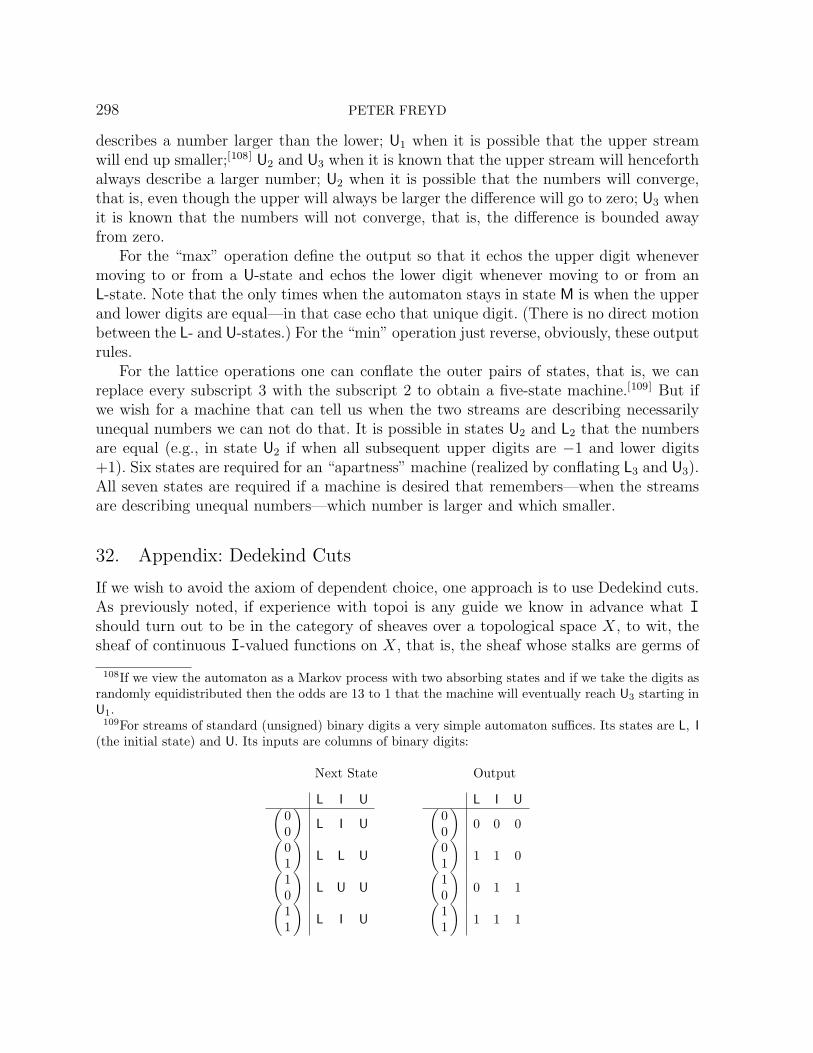
298 PETER FREYD

describes a number larger than the lower; U1 when it is possible that the upper streamwill end up smaller;[108] U2 and U3 when it is known that the upper stream will henceforthalways describe a larger number; U2 when it is possible that the numbers will converge,that is, even though the upper will always be larger the difference will go to zero; U3 whenit is known that the numbers will not converge, that is, the difference is bounded awayfrom zero.

For the “max” operation define the output so that it echos the upper digit whenevermoving to or from a U-state and echos the lower digit whenever moving to or from anL-state. Note that the only times when the automaton stays in state M is when the upperand lower digits are equal—in that case echo that unique digit. (There is no direct motionbetween the L- and U-states.) For the “min” operation just reverse, obviously, these outputrules.

For the lattice operations one can conflate the outer pairs of states, that is, we canreplace every subscript 3 with the subscript 2 to obtain a five-state machine.[109] But ifwe wish for a machine that can tell us when the two streams are describing necessarilyunequal numbers we can not do that. It is possible in states U2 and L2 that the numbersare equal (e.g., in state U2 if when all subsequent upper digits are −1 and lower digits+1). Six states are required for an “apartness” machine (realized by conflating L3 and U3).All seven states are required if a machine is desired that remembers—when the streamsare describing unequal numbers—which number is larger and which smaller.

32. Appendix: Dedekind Cuts

If we wish to avoid the axiom of dependent choice, one approach is to use Dedekind cuts.As previously noted, if experience with topoi is any guide we know in advance what Ishould turn out to be in the category of sheaves over a topological space X, to wit, thesheaf of continuous I-valued functions on X, that is, the sheaf whose stalks are germs of

108If we view the automaton as a Markov process with two absorbing states and if we take the digits asrandomly equidistributed then the odds are 13 to 1 that the machine will eventually reach U3 starting inU1.

109For streams of standard (unsigned) binary digits a very simple automaton suffices. Its states are L, I(the initial state) and U. Its inputs are columns of binary digits:

Next State Output

L I U(00

)L I U(

01

)L L U(

10

)L U U(

11

)L I U

L I U(00

)0 0 0(

01

)1 1 0(

10

)0 1 1(

11

)1 1 1

continuous functions (as defined in the topos of sets) from X to I. There are a numberof ways of define a Dedekind cut—all of them equivalent in the category of sets—but notall give give the right answer in a category of sheaves.

When working with I rather than D it is convenient to define Dedekind cuts as subsetsnot of I but of its “interior,” I

IIII

, the result of removing the two endpoints.[110]

We say that L ⊆ I

is a downdeal if:

` ∈ L ⇒ ∀`′<` `′ ∈ L

and it is an open downdeal if, further:

` ∈ L ⇒ ∃`′>` `′ ∈ L

We say that U is an updeal if

u ∈ U ⇒ ∀u′>u u′ ∈ U

and it is an open updeal if, further

u ∈ U ⇒ ∃u′<u u′ ∈ U

In the case of sheaves on X we may reinterpret L and U as a families of open subsets of Xindexed by elements of I

(that is, L` gives the “extent to which ` ∈ L”). The conditions

then rewrite to:L` =

⋃`′>`

L`′

Uu =⋃

u′ `

110Bear in mind that I and I

are isomorphic—as objects—to the natural numbers N. Another structurethat we will need is the free action generated by a two-element set (which will here usually be the twozooming operations). It comes equipped with one generator and two self-functions and is the initial objectin the category of such structures (it may be defined as the initial algebra for the functor that sends Xto 1+X +X). One may easily prove in topoi that for any object A the free A-action, A?, has a canonicalmonoid structure and as such it is the free monoid generated by A (the free A-action can be defined asthe initial algebra for the functor that sends X to 1+A×X). When A = 1+1 we have that (1+1)? is alsoisomorphic to N. Just in case one demands actual isomorphisms take (1 + 1)? ∼→ N to be the canonicalmap that sends the generator to the generator (i.e.,the empty word to zero) where the action of (1 + 1)on N is given by the pair of maps, the first of which sends n to 2n+1 and the second sends n to 2n+2.Take (1 + 1)? ∼→ I

to be the canonical map that sends the empty word to where the action is given

by the pair of maps, the first of which sends x to ⊥|x and the second sends x to >|x. (And, of course, Nis isomorphic to 1 + 1 + N, hence I

to I.)

300 PETER FREYD

and the largest open updeal contained in an updeal U is

U = u : ∃u′∈U u′ < u′

When working in sheaves these correspond to

L` =

⋃`′>`

L`′

Uu =

⋃u′] ∩ I

and for any upper semi-continuous g we obtain an open updeal

with Uu = g−1[⊥, u) ∩ I

. Conversely, given an open downdeal, L, define f(x) to besup ` : x ∈ L` and given an open updeal, U , define g(x) = inf u : x ∈ Uu . Itis easy to check that these assignments establish a correspondence between upper/lowersemi-continuous functions and open up/down-deals.

In the classical setting there are several ways of defining I: as the set of open downdeals;as the set of open updeals; as the set of pairs 〈L, U〉 where L is maximal among thosedowndeals disjoint from U and U is maximal among those disjoint from L. In the moregeneral setting, none of these are guaranteed to satisfy the separation condition: on anyspace X and open set V take L` to be constantly equal to V . The extent to which L is> is V and the extent to which it is different from > is ¬V , to wit, its exterior (definedas the largest open set disjoint from V , the interior of its complement). The extent towhich L is not ⊥ is ¬¬V (the interior of the closure of V ). The union ¬V ∪¬¬V fails, ingeneral, to be all of X. Note that the maximal open updeal disjoint from L is U whereUu is constantly ¬V . The maximal open downdeal disjoint from U is constantly ¬¬V . Ifwe take any adjoint pair of semi-continuous maps 〈f, g〉 and x ∈ X such that f(x) < g(x)we may let r = f(x)|g(x) and apply a suitable power of the dilatation at r to obtainan adjoint pair 〈(r/)nf, (r/)ng〉 that will recreate the same sort of pathology. We need, inother words. a condition on 〈L, U〉 that will force f = g.

Given any function h : X → I there is a maximal lower semi-continuous f : X → Ibelow h and a minimal upper semi-continuous g above h. (To obtain f first define adowndeal L by first taking L` to be the interior of h−1(`,>] and then replacing L` withL`.) Of course a function both upper and lower semi-continuous is plain continuous.

A Dedekind cut on I

is a pair of subsets 〈L, U〉 such that:L is an open downdeal:

` ∈ L ⇒ [∀`′<` `′ ∈ L] ∧ [∃`′>` `′ ∈ L]

U is an open updeal:

u ∈ U ⇒ [∀u′>u u′ ∈ U ] ∧ [∃u′<u u′ ∈ U ]

L and U disjoint:¬[q ∈ L ∧ q ∈ U ]

L and U almost cover:` ` L`′

` ) andUu = f−1[⊥, u). All Dedekind cuts so arise: given the L`s and Uus define f : X → I byf(x) = inf u : x ∈ Uu and verify that f is continuous (the key observation is that theclosure of Uu is contained in Uu′ whenever u < u′, hence x : f(x) ≤ u =

⋂u′>u Uu′ =⋂

u′>u Uu′ is closed and, dually, x : f(x) ≥ u is open).We define I to be the set of such Dedekind cuts. The bottom cut is 〈∅, I

〉; the top

cut is 〈I

, ∅〉.Note that 〈L, U〉 6= ⊥ iff L is non-empty and, dually, 〈L, U〉 6= > iff U is non-empty.

The almost-cover condition for the case ⊥ < > is precisely the separation condition forthe set of Dedekind cuts.

Define∨

〈L, U〉 = 〈 ∨` : > ` ∈ L , ∨

u : > u ∈ U 〉∧

〈L, U〉 = 〈 ∧` : < ` ∈ L , ∧

u : |`) < (>|u) we knowthat either (>|`) ∈ L or (>|u) ∈ U . In the first case ≤ (>|`)∧ ∈ L and in the secondcase < (>|u)∧ ∈ U .)

The disjointness condition for the case is precisely the continuous coalgebra condi-tion for these operations.

Given an interval coalgebra, C, satisfying the separation and continuous coalgebracondition, and given c ∈ C, we wish to construct a Dedekind cut 〈L(c), U(c)〉. By azooming sequence is meant an element of the free monoid on two generators, >-zoomingand ⊥-zooming.

` ∈ L(c) iff there is a zooming sequence α such that `α = ⊥ and ¬¬[c α = >].u ∈ U(c) iff there is a zooming sequence, α such that uα = > and ¬¬[c α = ⊥].

111L and U each determine the other: given L then U = u : ∃u′<uu′ 6∈ L . The axioms are, in fact,redundant: the 3rd and 4th conditions imply that L is a downdeal and U an updeal (but not the opennesscondition).

302 PETER FREYD

We need to verify the conditions for a Dedekind cut.Before doing so let us pause to collect a few easily verified observations in the intu-

itionistic setting. For any function, f , it is, of course, trivial that (x = y) ⇒ (fx = fy).Because negation is contravariant we also have (fx 6= fy) ⇒ (x 6= y) and ¬¬(x = y) ⇒¬¬(fx = fy). We will apply these trivial observations to the case when f is a zoomingsequence and incorporate the fact that > and ⊥ are fixed points. Hence

x = > ⇒ xα = >x = ⊥ ⇒ xα = ⊥

xα 6= > ⇒ x 6= >xα 6= ⊥ ⇒ x 6= ⊥

¬¬(x = ⊥) ⇒ ¬¬(xα = ⊥)¬¬(x = ⊥) ⇒ ¬¬(xα = ⊥)

We will also use these trivial consequences of the apartness of > and ⊥:

¬¬(x = ⊥) ⇒ x 6= >¬¬(x = ⊥) ⇒ x 6= ⊥

And we will freely use all sorts of nice properties enjoyed by I (including the discretecoalgebra condition).

Not so trivial is this critical lemma:

32.1. Lemma. For c ∈ C and u ∈ I the following conditions on c ∈ C and u ∈ I areequivalent:

α : ∃α[¬¬(c α = ⊥) ∧ (u α = >)]

β : ∃β[¬¬(c β = ⊥) ∧ (u β 6= ⊥)]

γ : ∃γ,v[(cγ 6= >) ∧ (v < u) ∧ (vγ = >)]

(Note that the γ-condition will tend be much more computationally feasible than theother two.)

α ⇒ γ :Given α let v be the unique element in I such that v α = and γ the result of following

α with a ⊥-zooming (and use (¬¬(c α = ⊥) ⇒ ¬¬(cγ = ⊥) ⇒ (cγ 6= >).)

γ ⇒ β :Given γ and v, We may assume that γ is the minimal zooming sequence for the task.

We know that it is non-empty since v < > and vγ = >. If γ ends with an >-zooming thenthe sequence obtained by removing that final >-zooming would work as well. Thus from itsminimality we may infer that γ ends with a ⊥-zooming. Let γ′ be the zooming sequenceobtained by removing that final ⊥-zooming. Since vγ′∨ = > we know that vγ′ ≥ ,hence uγ′ > and uγ′∧ 6= ⊥. Since c γ′∨ 6= > the continuous zooming condition says

that ¬¬[c γ′∧ = ⊥]. Thus we finish by defining β to be the result of following γ′ with an>-zooming.

β ⇒ α :Define α to be the result of following β with a sufficient number of ⊥-zoomings to

insure u α = >.Now for the Dedekind-cut conditions.

U(c) is an open updeal:Suppose u ∈ U(c). Let γ, v be such that cγ 6= >, v . Then for any

u′ > v we have the same three conditions with u′ instead of u, hence u′ ∈ U(c) for allu′ > v.

L(c) and U(c) almost cover:Given ` . The separation condition on C says that either cγ 6= >or cγ 6= ⊥. In the first case we have u ∈ U(c) and, dually, in the second case ` ∈ L(c).

L(c) and U(c) disjoint:We wish to reach a contradiction from the assumption that there is c ∈ A, q ∈ I and

zooming sequences σ, τ such that ¬¬(c σ = ⊥), qσ = >, ¬¬(c τ = >) and qτ = ⊥. We willsettle for a weaker condition: ¬¬(c σ = ⊥) implies c σ 6= > and ¬¬(c τ = >) implies c τ 6= ⊥.That is, we will reach a contradiction just from c σ 6= >, qσ = >, c τ 6= ⊥ and qτ = ⊥.

If σ were empty then q = > and it would not be possible for qτ = ⊥. Dually, τ is

non-empty. If σ were to start with >-zooming we would know that∧q 6= ⊥ forcing

∨q = >

(the discrete coalgebra condition holds in I) and thus qτ = >, contradicting qτ = ⊥. Hence

σ starts with ⊥-zooming and, dually, τ with >-zooming. From c σ 6= > we may infer∨c 6= >

and from c τ 6= ⊥ we infer∧c 6= ⊥. But the conjunctions of these two 6=s is precisely what

the continuous coalgebra condition says can not happen.We must show that this assignment of Dedekind cuts preserves the coalgebra structure.

There is no difficulty in showing that 〈L(⊥), U(⊥)〉 and 〈L(>), U(>)〉 are what they should

be. What we must show is 〈L(∧c), U(

∧c)〉 =

∧〈L(c), U(c)〉 (the other equation, of course, is

dual). Restated: we must show

∧` ∈ L(

∧c) iff ≤ ` ∈ L(c)

∧u ∈ U(

∧c) iff )

and∧`α

= ⊥ then if α′ is the result of following an >-zooming with α we have ¬¬(c α′= >)

112For example, k′ = `|u, v = k|u.

304 PETER FREYD

and ` α′= ⊥ (and if ` < then replace it with ). The same argument works when

∧u ∈ U(

∧c) (and since

∧u

α

= > we know that u > ).For the reverse direction, suppose ` ≥ , ¬¬(c α = >) and ` α = ⊥. Then α is necessar-

ily non-empty (that is, ` 6= ⊥) and it can not start with a ⊥-zooming (since ` ≥ implies∨` = >). Let α′ be the rest of the sequence after the initial >-zooming. Then ¬¬(

∧c α′

= >)

and∧` α′

= ⊥ forcing∧` ∈ L(

∧c)

Finally, suppose u > , ¬¬(cα = ⊥) and uα = >. If α is empty then the empty sequence

also establishes∧u ∈ U(

∧c). If α starts with a >-zooming we use the same sort of argument

just above to establish∧u ∈ U(

∧c). If α starts with a ⊥-zooming then for any u > it

is the case that uα = >, hence we need to show that everything in I other than ⊥ is in

U(∧a). But we may infer ¬¬(cα = ⊥) ⇒ (cα 6= ⊥) ⇒ (

∨c 6= ⊥) and the continuous coalgebra

condition says that ¬¬(∧c = >). For β the empty sequence we thus have ¬¬(

∧c

β

= >) and∧u

β

6= ⊥ forcing∧u ∈ U(

∧c).

33. Appendix: The Peneproximate origins

I always disliked analysis. Algebra, geometry, topology, even formal logic, they captivatedme; analysis was different.

My attitude, alas, wasn’t improved when I was supposed to tell a class of Princetonfreshmen about numerical integration. I was expected to tell them that the trapezoidrule was better than Riemann and that Simpson was better than trapezoids. I was notexpected to prove any of this.

I was appalled by the gap between applied mathematical experience and what we couldeven imagine proving. How does one integrate over all continuous functions to arrive atthe expected error of a particular method?

Of course one can carve out finite dimensional vector spaces of continuous functionsand compute an expected error thereon. But all continuous functions? It’s easy to provethat there is no measure—not even a finitely additive measure—on the set of all continuousfunctions assuming at least that we ask for even a few of the most innocuous of invarianceproperties. Yet experience said that there was, indeed, such a measure on the set offunctions one actually encounters.

But it wasn’t just a problem in mathematics: I learned from physicists that theysucceed in coming to verifiable conclusions by pretending to integrate over the set of allpaths between two points. Again it is not hard to prove that no such “Feynman integral”is possible once one insists on a few invariance properties.

Even later I learned (from the work of David Mumford) about “Bayesian vision”: inthis case one wants to integrate over all possible “scenes” in order to deduce the mostprobable interpretations of what is being seen. A scene is taken to be a function from, say,a square to shades of gray. It would be a mistake to restrict to continuous functions—sharpcontour boundaries surely want to exist. Quite remarkable “robotic vision” machines had


been constructed for specific purposes by judiciously cutting down to appropriate finite-dimensional vector spaces of scenes. But once again, there is no possible measure on setsof all scenes which enjoy even the simplest of invariance conditions.

Thus three examples coming with quite disparate origins—math, science, engineering—were shouting that we need a new approach to measure theory.

One line of hope arose from the observation that the non-existence proofs all require avery classical foundation. There’s the enticing possibility that a more computationally re-alistic setting—as offered, say, by effective topoi—could resolve the difficulties. A wonder-ful dream presents itself: the role of foundations in mathematics—and its applications—could undergo a transformation similar to the last two centuries’ transformation of geom-etry.

Geometry moved from fixed rigidity to remarkable flexibility and—in the last century—that liberal view became a critical tool in physics. We learned that there was a trade-offbetween physics and geometry; we could still insist on classical (Euclidean) geometry butonly at the expense of a cumbersome physics. We no longer even view most questionson the nature of geometry to be well put unless first the nature of physics be stipulatedand—of course—vice versa.

Could we now learn the same about foundations? Elementary topoi provide a generalsetting for shifting foundations in a manner similar to the role of Riemannian manifoldsin geometry. Might the trade-off between physics and geometry be replicated for physicsand foundations? Two hundred years ago there was only one geometry. It was more thantaken for granted; it was deemed to be certain knowledge.

Of course the geometry we now call Euclidean was certain; it may not be innate butit is inevitable. I have no doubt that if we lived in a universe with a visibly non-zerocurvature we would get around to building our blackboards with zero curvature.[113]

It must be deemed remarkable that we learned to think—and make correct predic-tions—in non-Euclidean geometry. We learned to imagine living in a 3-sphere, in spacesof higher genus, even in projective space. The representation theorems of Riemannianmanifolds (long before they were all proved) played a critical role in that process; and soit is with foundations. With a few topoi on hand for comparison, people do learn to shifttheir foundations between what’s called classical and what’s called (alas) intuitionistic.Again, the representation theorems play a critical role: in a fully classical setting a categoryof sheaves on a site can support a fully intuitionistic logic—change the topology on thecite and you can revert to the classical.

Coming back to earth: I must confess that the perfectly obvious idea that one shouldfirst establish ordinary integration in the right way on something as simple as the closedinterval, that simple idea took longer than it should have (it had to await a day’s boat tripin Alaska, of all places). For some years I preached this doctrine to the category/topos

113In this neighborhood, of course, Euclidean geometry is the natural geometry from the very beginning.When I was a kid a friend had measured the distance around a giant tree. We estimated the tree’s widthby solving the same problem on a little fruit-juice glass. We never questioned that the same ratio wouldhold for trees and glasses.

306 PETER FREYD

crowd and some trace of those preachings can be found scattered in the literature.[114]

In September 1999 at an invited talk at the annual ctcs meeting (held that year inEdinburgh) I even characterized the mean value of real-valued continuous functions onthe closed interval as an order-preserving linear operation that did the right thing toconstants and had the property that the mean value on the entire interval equaled themidpoint of the mean-values on the two half intervals. I described it with a diagram thatused (twice) the canonical equivalence between I and I ∨ I.

But one equivalence, even used twice, doesn’t bring forth the general notion: it doesn’tprompt one to invent ordered wedges; without ordered wedges one doesn’t define zoomoperators nor discover the theorem on the existence of standard models. One doesn’t learnhow remarkably algebraic real analysis can become.

What I needed was someone to kick me into coalgebra mode. Three months later twoguys did just that and on December 22 I wrote to the category list:

There’s a nice paper by Dusko Pavlovic and Vaughan Pratt. It’s entitledOn Coalgebra of Real Numbers [115] and it has turned me on.

A solution, alas, for the three motivating problems still awaits; but, at least, now Ilike analysis.

JJ

Department of Mathematics, University of PennsylvaniaPhiladelphia, PA, 19104Email: [email protected]

This article may be accessed at http://www.tac.mta.ca/tac/ or by anonymous ftp atftp://ftp.tac.mta.ca/pub/tac/html/volumes/20/10/20-10.dvi,ps,pdf

114e.g. Abbas Edalat and Martin Hotzel Escardo, Integration in real PCFLICS 1996, Part I (New Brunswick, NJ). Information and Computation 160 (2000), no. 1-2, 128–166).

115CMCS’99 Coalgebraic Methods in Computer Science (Amsterdam, 1999), 15 pp. (electronic)Electron. Notes Theor. Comput. Sci., 19, Elsevier, Amsterdam, 1999.

THEORY AND APPLICATIONS OF CATEGORIES (ISSN 1201-561X) will disseminate articles thatsignificantly advance the study of categorical algebra or methods, or that make significant new contribu-tions to mathematical science using categorical methods. The scope of the journal includes: all areas ofpure category theory, including higher dimensional categories; applications of category theory to algebra,geometry and topology and other areas of mathematics; applications of category theory to computerscience, physics and other mathematical sciences; contributions to scientific knowledge that make use ofcategorical methods.Articles appearing in the journal have been carefully and critically refereed under the responsibility ofmembers of the Editorial Board. Only papers judged to be both significant and excellent are acceptedfor publication.Full text of the journal is freely available in .dvi, Postscript and PDF from the journal’s server athttp://www.tac.mta.ca/tac/ and by ftp. It is archived electronically and in printed paper format.

Subscription information. Individual subscribers receive abstracts of articles by e-mail as theyare published. To subscribe, send e-mail to [email protected] including a full name and postal address. For in-stitutional subscription, send enquiries to the Managing Editor, Robert Rosebrugh, [email protected].

Information for authors. The typesetting language of the journal is TEX, and LATEX2estrongly encouraged. Articles should be submitted by e-mail directly to a Transmitting Editor. Pleaseobtain detailed information on submission format and style files at http://www.tac.mta.ca/tac/.

Managing editor. Robert Rosebrugh, Mount Allison University: [email protected]

TEXnical editor. Michael Barr, McGill University: [email protected]

Assistant TEX editor. Gavin Seal, Georgia Southern University: gavin [email protected]

Transmitting editors.Richard Blute, Universite d’ Ottawa: [email protected] Breen, Universite de Paris 13: [email protected] Brown, University of North Wales: ronnie.profbrown (at) btinternet.comAurelio Carboni, Universita dell Insubria: [email protected] de Paiva, Xerox Palo Alto Research Center: [email protected] Getzler, Northwestern University: getzler(at)northwestern(dot)eduMartin Hyland, University of Cambridge: [email protected]. T. Johnstone, University of Cambridge: [email protected] Kock, University of Aarhus: [email protected] Lack, University of Western Sydney: [email protected]. William Lawvere, State University of New York at Buffalo: [email protected] Loday, Universite de Strasbourg: [email protected] Moerdijk, University of Utrecht: [email protected] Niefield, Union College: [email protected] Pare, Dalhousie University: [email protected] Rosicky, Masaryk University: [email protected] Shipley, University of Illinois at Chicago: [email protected] Stasheff, University of North Carolina: [email protected] Street, Macquarie University: [email protected] Tholen, York University: [email protected] Tierney, Rutgers University: [email protected] F. C. Walters, University of Insubria: [email protected]. J. Wood, Dalhousie University: [email protected]

algebraic real analysis - mount allison university · algebraic real analysis 217 denote a...

Documents