algebraic system analysis of timed petri netsgaubert/papers/cgq95-… · · 1996-10-04problems...
TRANSCRIPT

Algebraic System Analysis of TimedPetri Nets
G. Cohen, S. Gaubert and J. P. Quadrat
August 2, 1995To appear in \Idempotency}, J. Gunawardena Ed.
Collection of the Isaac Newton Institute, Cambridge University Press
Abstract
We show that Continuous Timed Petri Nets (CTPN) can be modeled bygeneralized polynomial recurrent equations in the (min,+) semiring. We es-tablish a correspondence between CTPN and Markov decision processes.We survey the basic system theoretical results available: behavioral (input-output) properties, algebraic representations, asymptotic regime. A particu-lar attention is paid to the subclass of stable systems (with asymptotic lineargrowth).
1 Introduction
The fact that a subclass of Discrete Event Systems equations write linearly in the(min,+) or in the (max,+) semiring is now almost classical [9, 2]. The (min,+) lin-earity allows the presence of synchronization and saturation features but unfortu-nately prohibits the modeling of many interesting phenomena such as “birth” and“death” processes (multiplication of tokens) and concurrency. The purpose of thispaper is to show that after some simplifications, these additional features can berepresented by polynomial recurrences in the (min,+) semiring.
We introduce a fluid analogue of general Timed Petri Nets (in which the quanti-ties of tokens are real numbers), called Continuous Timed Petri Nets (CTPN). Weshow that, assuming a stationary routing policy, the counter variables of a CTPNsatisfy recurrent equations involving the operators min;+;�. We interpret CTPNequations as dynamic programming equations of classical Markov Decision Prob-lems: CTPN can be seen as the dedicated hardware executing the value iteration.
We set up a hierarchy of CTPN which mirrors the natural hierarchy of optimiza-tion problems (deterministic vs. stochastic, discounted vs. ergodic). For each leveland sublevel of this hierarchy, we recall or introduce the required algebraic and an-alytic tools, we provide input-output characterizations and give asymptotic results.
The paper is organized as follows. Inx2, we give the dynamic equations satisfiedby general Petri Nets under the earliest firing rule. The counter equations given here

2 G. Cohen, S. Gaubert and J. P. Quadrat
are much more tractable than the dater equations obtained previously [1]. Similarequations have been introduced by Baccelli et al. [3] in a stochastic context.
In x3, we introduce the continuous analogue of Timed Petri Nets. We discussvarious natural routing policies, and show that they lead to simple recurrent equa-tions.
In x4, we present the first level of the hierarchy: Continuous Timed EventGraphs with Multipliers (CTEGM), characterized by the absence of routing de-cisions. We single out several interesting subclasses. 1. Ordinary Timed EventGraphs (TEG) are probably the simplest and best understood class of Timed Dis-crete Event Systems. TEG are exactly causal finite dimensional recurrent linearsystems over the (min,+) semiring. They correspond to deterministic decisionproblems with finite state and additive undiscounted cost. Their asymptotic theoryis mere translation of the (min,+) spectral theory. Their input-output relations areinf-convolutions with (min,+) rational sequences. 2. We introduce the subclass ofCTEGM with potential, which reduce to TEG after a change of units (they are lin-earized by a non linear change of variable in the (min,+) semiring). The importanceand tractability of the (non continuous) version of these systems, called expansible[23] was first recognized by Munier. 3. �-discounted TEG are the TEG-analogueof uniformly discounted deterministic optimization problems. They represent sys-tems with constant birth (or death) rate �. 4. We consider general CTEGM. Theirinput-output relations are affine convolutions (minima of affine functions of thedelayed input). The transfer operators are rational series with coefficients in thesemiring of piecewise affine concave monotone maps. To CTEGM correspond de-terministic decision problems where the actualization rate (and not only the transi-tion cost) is controlled. Last, certain routing policies, called injective, reduce CTPNto CTEGM. Related resource optimization problems (optimizing the allocation ofthe initial marking) are discussed in x4.7.
In x5, we examine the second level of the hierarchy: general CTPN, which cor-respond to stochastic decision problems. Algebraically, CTPN are (min,+) polyno-mial systems whose outputs admit Volterra series expansions. They are character-ized by simple behavioral properties (essentially monotonicity and concavity). Wefocus on the following tractable subclasses. 1. Undiscounted TPN are the Petri Netanalogue of stochastic control problems with undiscounted (ergodic) cost. They arecharacterized by a structural condition (as many input as output arcs at each place)plus a compatibility condition on routings. Undiscounted TPN admit an asymptot-ically linear growth. The asymptotic behavior can be obtained by transferring theresults known for the value iteration: we give a “critical circuit” formula similarto the TEG case (the circuits have to be replaced by recurrent classes of station-ary policies). 2. Similar results exist for TPN with potential (obtained from undis-counted TPN by diagonal change of variable). 3. CTPN with fixed birth/death rate� correspond to the well studied class of discounted Dynamic Programming recur-rences.

Algebraic System Analysis of Timed Petri Nets 3
2 Recurrent Equations of Timed Petri Nets
p1
p2
q1 q2 q3
q5 q6 q4
Figure 1: Notation for Petri Nets. P = fp1; p2g, Q = fq1; : : : ; q6g, pout1 =
fq1; q4; q5g, pin1 = fq1; q2; q3g, pout
2 = fq5; q6g, Mq5p1 = 2, Mp1q2 = 3, mp1 = 3,mp2 = 1.
Definition 2.1 (TPNM). A Timed Petri Net with Multipliers (TPNM) is a valuedbipartite graph given by a 5-tuple N = (P;Q;M;m; � ).
1. The finite set P is called the set of places. A place may contain tokens whichtravel from place to place according to a firing process described later on.
2. The finite set Q is called the set of transitions. A transition may fire. When itfires, it consumes and produces tokens.
3. M 2 NP�Q[Q�P . Mpq (resp. Mqp) gives the number of edges from transition qto place p (resp. from place p to transition q). In particular, the zero value forM corresponds to the absence of edge.
4. m 2 NP : mp denotes the number of tokens being initially in place p (initial
marking).
5. � 2 NP : �p gives the minimal time a token must spend in place p before be-
coming available for consumption by downstream transitions1. It will be calledholding time of the place throughout this paper.
We denote by rout the set of vertices (places or transitions) downstream a vertexr and rin the set of vertices upstream r. Formally,
rout = fs j Msr 6= 0g; rin = fs j Mrs 6= 0g :
In order to specify a unique behavior of the system, we equip TPN with routingpolicies.
Definition 2.2 (Routing Policy). A routing policy at place p is a familyfmqp;�
p
qq0gq2pout;q02pin , where,
1. mp =P
q2pout mqp is an integer partition of the initial marking. mqp tells thenumber of tokens of the initial marking reserved for transition q.
1Without loss of modeling power, the firing of transitions is supposed to be instantaneous (i.e.it involves no delay in consuming and producing tokens).

4 G. Cohen, S. Gaubert and J. P. Quadrat
2. f�p
qq0gq2pout is a partition of the flow from q0. That is, �p
qq0(n) tells the numberof tokens routed from q0 to q via p among the first n ones. More formally, �p
qq0
are nondecreasing maps N! N such that 8n,P
q2pout �p
qq0(n) = n.
A routing policy for the net is a collection of routing policies for places.
Then, the earliest behavior of the system is defined as follows. As soon as atoken enters a place, it is reserved for the firing of a given downstream transitionaccording to the routing policy. A transition q must fire as soon as all the places pupstream q contain enough tokens (Mqp) reserved for transition q and having spentat least �p units of time in place p (by convention, the tokens of the initial mark-ing are present since time �1, so that they are immediately available at time 0).When the transition fires, it consumes the corresponding upstream tokens and im-mediately produces an amount of tokens equal toMpq in each place p downstreamq.
We next give the dynamic equations satisfied by the Timed Petri Net. We as-sociate counter functions to nodes and arcs of the graph: Zp(t) denotes the cumu-lated number of tokens which have entered place p up to time t, including the ini-tial marking; Zq(t) denotes the number of firings of transition q having occurred upto time t; Wpq(t) denotes the cumulated number of tokens arrived at place p fromtransition q up to time t; Wqp(t) denotes the cumulated number of tokens arrived atplace p up to time t (including the initial marking) reserved for the firing of transi-tion q. We introduce the notation
�pqdef= Mpq; �qp
def= M�1
qp ;
and we set bxc = supfn 2 Zj n � xg.
Assertion 2.3. The counter variables of a Timed Petri Net under the earliest firingrule satisfy the following equations2
Zq(t) = minp2qin
b�qpWqp(t� �p)c ; (2.1a)
Wpq(t) = �pqZq(t) ; (2.1b)
Zp(t) = mp +Xq2pin
Wpq(t) ; (2.1c)
Wqp = mqp +Xq02pin
�p
qq0(Wpq0) : (2.1d)
We deduce from (2.1) the transition-to-transition equation
Zq(t) = minp2qin
j�qp
�mqp +
Xq02pin
�p
qq0
��pq0Zq0(t� �p)
��k: (2.2)
2We adopt the conventionP
q2;() = 0, so that (2.1c) becomes Zp(t) = mp when pin= ;.
The transitions q such that qin= ; will be considered as input transitions whose behavior is given
externally. Thus, Eq. (2.1a) should be ignored whenever q has no predecessors.

Algebraic System Analysis of Timed Petri Nets 5
If �p = 0 for some places, this equation becomes implicit and we may have diffi-culties in proving the existence of a finite solution. We say that the TPN is explicitif there is no circuits containing only places with zero holding times. This ensuresthe uniqueness of the solution of (2.1) and (2.2) under any routing policy �.
Input-Output Partition We partition the set of transitionsQ = U[X [Y whereU is the set of transitions with no predecessors (input transitions), Y is the set oftransitions with no successors (output transitions) and X = Q n (U [ Y). We de-note by u (resp. x, y) the vector of input (resp. state, output) counters Zq; q 2 U
(resp. X , Y). Throughout the paper, we will study the input-output behavior of thesystem. That is, we look for the minimal trajectory (x; y) generated by the inputhistory u(t); t 2 Z. This encompasses the autonomous regime traditionally con-sidered in the Petri Net literature, when the system is frozen at an initial conditionZq(t) = vq 2 R for negative t, and evolves freely according to the dynamics (2.1)for t � 0. This can be obtained as a specialization of the input-output case by ad-joining an input transition q0 upstream each original transition q, setting uq0(t) = vqfor t < 0, uq0(t) = +1 otherwise.
3 Modeling of Continuous Timed Petri Nets
We shall address the continuous version of TPN (in which the number of tokens arereal numbers instead of integers). Such continuous models occur naturally whenfluids rather than tokens flow in networks (see [2, x1.2.7],[24] for an elementaryexample). They also arise as approximation of (discrete) Petri Nets since they pro-vide an upper bound for the real behavior.
A continuous TPN (CTPN) is defined as a TPN, but the marking m, the mul-tipliers M and the counter functions are real-valued (the multipliers must be non-negative: Mrs 2 R
+). This allows one to define some simple stationary routingpolicies. We shall single out three classes of policies.
General Stationary Routing A stationary routing policy is of the form�
p
qq0(n) = �p
qq0 � n for some constants �pqq0 � 0 such that for all q0 2 pin,Pq2pout �
p
qq0 = 1 That is, the flow from q0 at place p goes to q with proportion �pqq0 .The counter functions of a CTPN satisfy the following equations
Zq(t) = minp2qin
�qpWqp(t� �p) ; (3.1a)
Wqp(t) = mqp +Xq02pin
�p
qq0Wpq0(t) ; (3.1b)
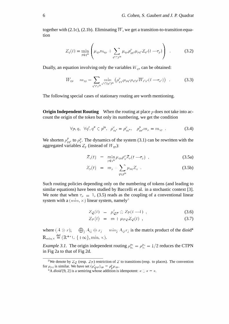
6 G. Cohen, S. Gaubert and J. P. Quadrat
together with (2.1c), (2.1b). EliminatingW , we get a transition-to-transition equa-tion
Zq(t) = minp2qin
0@�qpmqp +
Xq02pin
�qp�p
qq0�pq0Zq0(t� �p)
1A : (3.2)
Dually, an equation involving only the variables Wqp can be obtained:
Wqp = mqp +Xq02pin
minp02(q0)in
��p
qq0�pq0�q0p0Wq0p0(t� �p0)
�: (3.3)
The following special cases of stationary routing are worth mentioning.
Origin Independent Routing When the routing at place p does not take into ac-count the origin of the token but only its numbering, we get the condition
8p; q; 8q0; q00 2 pin; �pqq0 = �pqq00; �pqq0mp = mqp : (3.4)
We shorten �pqq0 to �pq . The dynamics of the system (3.1) can be rewritten with theaggregated variables Zp (instead of Wqp):
Zq(t) = minp2qin
�qp�pqZp(t� �p) ; (3.5a)
Zp(t) = mp +Xq2pin
�pqZq : (3.5b)
Such routing policies depending only on the numbering of tokens (and leading tosimilar equations) have been studied by Baccelli et al. in a stochastic context [3].We note that when �p � 1, (3.5) reads as the coupling of a conventional linearsystem with a (min;�) linear system, namely3
ZQ(t) = �0QP ZP(t� 1) ; (3.6)
ZP(t) = m+ �PQZQ(t) ; (3.7)
where (A x)i =L
j Aij xj = minj Aijxj is the matrix product of the dioid4
Rmin;�def= (R+� [ f+1g;min;�).
Example 3.1. The origin independent routing �p5q3 = �p5q4 = 1=2 reduces the CTPNin Fig 2a to that of Fig 2d.
3We denote by ZQ (resp. ZP) restriction of Z to transitions (resp. to places). The conventionfor �pq is similar. We have set (�0QP)qp = �pq�qp.
4A dioid [9, 2] is a semiring whose addition is idempotent: a� a = a.

Algebraic System Analysis of Timed Petri Nets 7
(b)
(c)
(a)
(d)
Marking mq4 p 5Marking mq3 p5
Marking m p 5
f p5(q4 ) =
q1
f p5(q3 ) =
q2
q3
p3 p1 p2 p4
p3 p1 p5 p2 p4
q4
q1 q2
q1 q2
q3 q4
p3 p1 p2 p4
q1 q2
q3 q4
p3 p1 p2 p4
q1 q2
q3 q4
f p 5 (q4 ) = q2
f p 5 (q3 ) = q1
Origin independent routing
Bijective routing
Bijective routing
Figure 2: A Balanced Petri Net under various Routing Policies
Injective Routing We say that the routing function �p at place p is injective ifthere is a map fp : pout ! pin such that
8q; �p
qq0 6= 0) q0 = fp(q) : (3.8)
That is, all the tokens routed to q at place p come for a single transition f(q). Suchroutings occur frequently when tokens correspond to resources (e.g. pallets) whichfollow some well defined physical routes. An injective routing exists iff5 jpoutj �
jpinj. Indeed, the following stronger condition is often satisfied in practice (e.g. inFig. 2a).
Definition 3.2 (Balanced TPN). A TPN is balanced if 8p, jpjout = jpjin.
In this particular case, we shall speak of bijective routing policies (since fp be-comes a bijection pout ! pin). We shall see later on that injective and bijectiverouting policies lead to tractable classes of systems.
4 Timed Event Graphs and (min,+) Linear Systems
4.1 Ordinary and Generalized Timed Event Graphs
Definition 4.1 (Timed Event Graphs). A Continuous Timed Event Graph withMultipliers (CTEGM) is a CTPN such that there is exactly one transition upstreamand one transition downstream each place. An (ordinary) Continuous Timed Event
5We denote by jXj the cardinal of a set X.

8 G. Cohen, S. Gaubert and J. P. Quadrat
Graph (CTEG) is a CTEGM such that all arcs have multiplier one: Mpq;Mqp 2
f0; 1g. More generally, we define the place multipliers6
�pdef= �poutp�ppin : (4.1)
A (rate �)-CTEG is a CTEGM with unit holding times and constant place multipli-ers. A CTEGM admits a potential if there exists a vector v 2 (R+�)Q[P (potential)such that
8r; s 2 Q[ P; r 2 sout ) vr = �rsvs : (4.2)
We set
�pdef= �poutpmp : (4.3)
Assertion 4.2. The dynamics of a CTEGM writes
Zq(t) = minp2qin
��p + �pZpin(t� �p)
�: (4.4a)
We have the following specializations:
Zq(t) = minp2qin
��p + Zpin(t� �p)
�(TEG case), (4.4b)
Zq(t) = minp2qin
��p + �Zpin(t� 1)
�(rate � case), (4.4c)
Zq(t) = vqminp2qin
�v�1p mp + v�1
pin Zpin(t� �p)�
(Potential case). (4.4d)
The last equation shows that CTEGM with potential reduces to ordinary CTEGafter the diagonal change of variable Zq = vqZ
0q . This change of variables should
be interpreted as a change of units (vq firings of transition q being counted as a singleone).
Example 4.3. If one mixes white and red paints in equal proportions to producepink paint, the main concern is to say that with 3 liters of red for a single liter ofwhite, there is 2 liters of red which are useless (that is, the min is the appropriateoperator) but then 2 liters of pink can be produced, hence the right thing to do is tocount pink paint by pairs of liters.
Theorem 4.4. CTPN under injective routing policies reduce to CTEGM. BalancedCTPN with unit multipliers reduce to (ordinary) TEG.
Proof. Define the new set of placesP 0 = Q�P , with the incidence relation qin =
f(qp) j p 2 ping, (qp)in = fp(q). Then, the dynamics (3.2) reduce to (4.4a), with�qp = �qp�pfp(q), The specialization to the TEG case is immediate.
Example 4.5. The Petri Net of Figure 2a admits two possible bijective routing poli-cies at place p5 which lead to the two Timed Event Graphs of Fig. 2b and 2c respec-tively.
6Since pout and pin are singletons, the notation will be used to designate their single members.

Algebraic System Analysis of Timed Petri Nets 9
4.2 Dynamic Programming Interpretation of CTEGM
We exhibit a correspondence between the above classes of Event Graphs and clas-sical deterministic decision problems.
Given a CTEGM, we consider the discrete time controlled process qn over anhorizon t with
1. finite state space Q;
2. set of admissible control histories Pad = fp1; : : : ; pt j 8n; pn 2 qinn g;
3. backward dynamics qn�1 = pinn where pn 2 qin
n .
In other words, the controlled process follows the edges of the net with the reverseorientation, backward in time. The control at state (transition) q consists in choos-ing a place p upstream q, which leads to the (unique) transition q0 upstream p.
We shall consider the following 3 deterministic cost structures.
Additive
J add(p; t) = Z(0)q0 +
tXn=1
�pn : (4.5)
Note that the initial costZ(0) coincides with the initial value of the counter functionof the CTEGM.
Additive with Constant Discount Rate
Jdisc(p; t) = �tZ(0)q0 +
tXn=1
�t�n�pn : (4.6)
Additive with Controlled Discount Rate
J c-disc(p; t) =
tY
j=1
�pj
!Z(0)q0 +
tXn=1
tY
j=n+1
�pj
!�pn : (4.7)
The value function associated with any of the above cost functions J is the map
Zq(t) = minp2Pad; qt=q
J(p; t) :
Theorem 4.6. When �p � 1,
1. The counter of a CTEG coincides with the value function for the additive costJ add.
2. The counter of a (rate �)-CTEG coincides with the value function for the dis-counted cost Jdisc.

10 G. Cohen, S. Gaubert and J. P. Quadrat
3. The counter of a CTEGM coincides with the value function for the cost with con-trolled discount rate J c-disc.
Remark 4.7. Minimizing J c-disc is known as a problem of shortest path with gains.See [17, Chap. 3, x7] and the references therein.
4.3 Operatorial Representation of CTEGM
We introduce the set of signals Sdef= (R[ f+1g)Zto represent counter functions
(although this will be the case in most applications, we do not require the signalsto be either positive valued or nondecreasing).
Definition 4.8. An operator f : S ! S is
1. additive if it satisfies the min–superposition property
f(min(x; x0)) = min(f(x); f(x0)) ; (4.8)
2. linear if it is additive and satisfies the homogeneity property
f(� + x) = �+ f(x) :
Of course, “linear” refers to the (min,+) dioid Rmindef= (R [ f+1g;min;+).
Throughout the paper, we shall freely use the dioid notation a � b for min(a; b),a b for a+ b, " = +1 for the zero element, e = 0 for the unit.
The following 3 families of operators play a central role in CTEGM:
� : �x(t)def= x(t) + � (shift in counting)
�� : ��x(t)def= x(t� � ) (shift in dating)
� : �x(t)def= � � x(t) (scaling),
(4.9)
where � 2 R; � 2 N; � 2 R+�. We note that and � are linear while � is only
additive. We have the commutation rules:
��� = �� � ; (4.10a)
��� = ��� ; (4.10b)
� � = ��� : (4.10c)
Additive operators equipped with pointwise min and composition form an idempo-tent semiring, that we denote by O. The following subsemirings ofO are central.
1. The semiring generated by � ; � 2 R is isomorphic toRmin via the identificationof � to � .
2. The semiring generated by � ; �� ; � 2 R; � 2 R is isomorphic to the semiringof polynomials in the indeterminate �,Rmin[�] (via the same identification).

Algebraic System Analysis of Timed Petri Nets 11
3. The semiring generated by � ; � 2 R+ and by the powers of ��, where � is agiven and fixed value of�, will be denoted byRmin[��]. It is a particular instanceof a classical structure in difference algebra: Ore polynomials7 [26, 19, 13].
4. The semiring generated by �; �; � 2 R; � 2 R+� is isomorphic to the semiringof nondecreasing concave piecewise affine maps R [ f+1g ! R [ f+1g,that we denote by Amin. A generic element inAmin is a map p =
Lk
i=1 �i �i ,
p(x) = min1�i�k
(�i + �ix) :
5. Finally, the semiring generated by � ; ��; �; � 2 R; � 2 N; � 2 R+� is isomor-phic to the semiring of polynomialsAmin[�] .
We extend the operatorial notation to matrices by setting forA 2 On�p and x 2 Sp,
(Ax)idef= min
jAij(xj) : (4.11)
Note that for operator matricesA;A0; B and vectors of counters x; x0 of appropriatesizes
(AB)x = A(Bx); (A�A0)x = Ax�A0x; A(x� x0) = Ax�Ax0 :;
More formally, vectors of counter functions are a left semimodule under the actionof additive matrix operators.
Theorem 4.9. The counter equations of a CTEGM write
x = Ax�Bu; y = Cx�Du (4.12)
where A;B;C;D are matrices with entries inO. More precisely,
1. the entries of A;B;C;D belong to Rmin[�] for an ordinary CTEG;
2. the entries belong to Rmin[��] for a (rate �)-CTEG;
3. the entries belong to Amin[�] for a general CTEGM.
7We recall that given a semiring S equipped with an automorphism � : S ! S, the semiringof Ore polynomials in the indeterminate X, denoted by S[X;�], is the set of finite formal sumsP
n snXn (all but a finite number of sn are zero), equipped with the usual componentwise sum
(s � s0)ndef= sn � s0n and the skew Cauchy product (s s0)n
def=L
p+q=n sp �p(sq). This
product is determined by the rule Xa = �(a)X for all a 2 S. IdentifyingX with �� and setting
�(�)def= � � � for � 2 Rmin, we see that X� = �(�)X is nothing but the rule �� � = ����
which follows from (4.10).

12 G. Cohen, S. Gaubert and J. P. Quadrat
Theorem 4.10 (Convolution Representation). An explicit SISO8 CTEGM ad-mits an input output relation of the form
y(t) = inf�2N
[h(� ) + u(t� � )] (Ordinary CTEG) (4.13)
y(t) = vy inf�2N
[h(� ) + v�1u u(t� � )] (CTEG with potential) (4.14)
y(t) = inf�2N
[h(� ) + ��u(t� � )] (CTEG with rate �) (4.15)
y(t) = infi2I
[�i + �iu(t� �i)] (General Case) (4.16)
where h is a map N ! R [ f+1g, vu; vy 2 R+�, and where the family f�i 2
R; �i 2 R+�; �i 2 Ng is such that there is only finitely many i such that �i = � for
any � 2 N.
We postpone the proof: these representation results will appear as consequencesof the more general behavioral properties of CTEGM operators given in x4.4.
Theorem 4.9 established a connection between various algebras of polynomialtype and various classes of Event Graphs. Theorem 4.10 now establishes a simi-lar connection between input-output representations and certain formal series alge-bras. Let us recall that given a semiring K and an indeterminate �, we denote byK[[�]] the semiring of series with coefficients in K (set of formal sums
Lt2Nht�
t
with ht 2 K, equipped with pointwise sum and Cauchy product). The generic se-ries of Amin[[�]] writes
h =M�2N
h��� =
M�
Mi2I�
�i� �i�
!��
where for all � , I� is finite. Such series act naturally on S by interpreting the inde-terminate � as the shift operator
hu(t) =M�2N
h� (u(t� � )) = inf�2N
mini2I�
(�i� + �i�u(t� � )) :
Theorem 4.10 asserts that (i)- CTEGM operators correspond to the action ofAmin[[�]] on counter functions, (ii)- CTEG operators correspond to the action ofRmin[[�]], (iii)- �-CTEG operators correspond to the action of the dioid of Ore se-ries Rmin[[��]] (defined as Ore polynomials, without the finiteness condition).
4.4 Behavioral Characterizations of CTEGM
Theorem 4.11. The input-output map H : u! y of a SISO explicit CTEGM sat-isfies the following properties.
8Single Input-Single Output. The extension to the Multiple Inputs Multiple Outputs (MIMO)case is immediate.

Algebraic System Analysis of Timed Petri Nets 13
1. Stationarity. H�� = ��H.
2. Causality. u(t) = v(t);8t� � ) 8t � �; Hu(t) = Hv(t).
3. Additivity. H(min(u; v)) = min(Hu;Hv).
4. Scott continuity. For any filtered9 family fuigi2I , H(infi2I ui) = infi2IHui.
5. Concavity. H(Pn
i=1 �iui) �P
i �iHui, 8�i � 0;P
i �i = 1.
A CTEG with rate � satisfies the additional property
6. �-homogeneity. For all constant �, H(��t + u) = ��t +Hu, with an obviousconvention10.
A CTEGM with potential satisfies the alternative additional property11
7. (vu; vy)-homogeneity. For all � 2 R,H(�vu + u) = �vy +H(u).
Note that the specialization of the �-homogeneity to � = 1 gives the standardhomogeneity property � + u ! � + y. So does the specialization of the (vu; vy)-homogeneity to the case of constant potential v.
Proof. The additivity of H is an immediate consequence of the additivity ofA;B;C;D and the uniqueness of the solution of x = Ax � Bu; y = Cx � Du.The other properties can be proved along the same lines by transferring to H theproperties valid for A;B;C;D.
The following converse theorem shows that the properties listed are accurate.
Theorem 4.12. A mapH which satisfies properties 1–5 in Theorem 4.11 is a non-increasing limit of CTEGM operators12. An operator which satisfies 1–6 (resp. 1–5,7) is a nonincreasing limit of rate � CTEG operators (resp. with potential v).
The main point of the proof consists in the following general “convolution” rep-resentation lemma for additive continuous stationary operators.
Lemma 4.13. Let D denote a complete13 dioid,H : DZ! DZ. The following as-sertions are equivalent. 1.H is stationary, causal, additive, and Scott continuous;
9A family is filtered if any finite subfamily admits a lower bound in the family. Note thatthe Scott continuity together with additivity is equivalent to the preservation of arbitrary inf:H(infi ui) = infiHui for an arbitrary family. The Scott topology is presented in details in [16].What we call here Scott continuity is in fact Scott continuity with respect to the algebraic order �of the (min,+) semiring, defined by a � b () a � b = b ( which is reversed with respect tonatural order).
10�t denotes the map t 7! �t.11�+ u denotes the signal t 7! � + u(t).12I.e. there exists a nonincreasing sequence Hi � Hi+1; i 2 N of input-output operators of
CTEGM such thatH = infi2I Hi.13A dioid D is complete if an arbitrary subset admits a least upper bound (for the order a �
b () a� b = b) and if the product is Scott continuous.
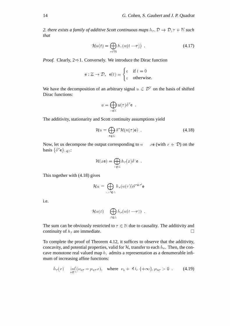
14 G. Cohen, S. Gaubert and J. P. Quadrat
2. there exists a family of additive Scott continuous maps h� ;D ! D; � 2 N suchthat
Hu(t) =M�2N
h� (u(t� � )) : (4.17)
Proof. Clearly, 2)1. Conversely. We introduce the Dirac function
e :Z! D; e(t) =
(e if t = 0
" otherwise.
We have the decomposition of an arbitrary signal u 2 DZon the basis of shiftedDirac functions:
u =M�2Z
u(� )��e :
The additivity, stationarity and Scott continuity assumptions yield
Hu =M�2Z
��H(u(� )e) : (4.18)
Now, let us decompose the output corresponding to u = xe (with x 2 D) on thebasis f��eg�2Z:
H(xe) =M�2Z
h� (x)��e :
This together with (4.18) gives
Hu =M�;� 02Z
h� (u(� ))��+� 0
e
i.e.
Hu(t) =M�2Z
h� (u(t� � )) :
The sum can be obviously restricted to � 2 N due to causality. The additivity andcontinuity of h� are immediate.
To complete the proof of Theorem 4.12, it suffices to observe that the additivity,concavity, and potential properties, valid forH, transfer to each h� . Then, the con-cave monotone real valued map h� admits a representation as a denumerable infi-mum of increasing affine functions:
h�(x) = infn2N
(�n� + �n�x); where �n 2 R[ f+1g; �n� > 0 : (4.19)

Algebraic System Analysis of Timed Petri Nets 15
The operator Hn =L
��n;k�n �k��k��
� arises from a CTEGM operator (sinceit obtained by a finite number of parallel/series composition of elementary ; �; �operators). It follows from (4.17)–(4.19) that limn # Hnu = Hu. This proves thefirst assertion of Theorem 4.12. The �-rate and potential special cases are imme-diate.
Finally, we note that the construction of the above proof explicitly yields theconvolution representations stated in Theorem 4.10, with the exception of the ad-ditional finiteness condition that h� is a finite sum of �i�i. This last result stemsfrom the rationality features that we next introduce.
4.5 Rational Operators
A natural problem is to characterize the subclass of series ofAmin[[�]]which arise astransfer operators of CTEGM (called transfer series). We recall that given a semir-ing of formal seriesK[[�]], the semiring of rational series [4] denoted byKrat[[�]] isthe least subsemiring containing polynomials and stable by the operation�;; �,
where a�def=L
n2Nan is defined only on series with zero constant coefficient. An
immediate fixed-point argument14 shows that the input and output counters givenby (4.12) satisfy y = hu, where h = CA�B �D is the transfer series of the sys-tem. Therefore, rephrasing the Kleene-Schutzenberger theorem [4], we claim thattransfer series and rational series coincide.
Assertion 4.14. The transfer series of explicit SISO CTEGM (resp. �-CTEG,CTEG) are precisely the elements ofArat
min[[�]] (resp. Rratmin[[��]],R
ratmin[[�]]).
One important problem is to characterize these particular classes of rational se-ries. The answer is known in the case of Rmin[[�]] and Rmin[[��]]. We say that aseries is ultimately periodic with rate � if there exists a constant � and a positiveinteger c (cyclicity) such that for t large enough
ht+c = �1 � �c
1� �+ �cht : (4.20)
When � < 1, this periodicity property means that ht converges towards �=(1��)
with rate � and that the rate is attained exactly after a finite time. The specializa-tion to � = 1 (in fact, � = 1�) yields ht+c = �c + ht. The merge of k seriesh(0); : : : ; h(k�1) is the series with coefficients hi+nk = h
(i)n for 0 � i � k � 1; n 2
N.
Theorem 4.15. A series in Rmin[[��]] is rational iff it is a merge of ultimately �-periodic series.
14The unique solution of x = Ax� Bu is x = A�Bu. The existence of A� and the uniquenessof the solution follow from the assumption that there are no circuits with zero holding times.

16 G. Cohen, S. Gaubert and J. P. Quadrat
The CTEG case (i.e. � = 1) is proved in [9, 2] for the subclass of monotone15
series hn+1 � hn. It was already noticed by Moller [22] in the non monotone case.It is essentially known to the tropical community [20]. The �-generalization wasannounced in [13]. The proof will appear in a paper in preparation [15].
No such simple characterization seems to exist forAratmin[[�]]: the coefficient h�
of �� in h is an element of Amin, but its complexity16 grows in general as � !1.
4.6 Asymptotic Behavior of CTEGM
We consider the autonomous case Z = AZ with boundary condition 8t �
0; Z(t) = v 2 RQ, where A belongs to one of the above matrix operator algebras.We associate several additive weights with the circuit C = (q1; p1; q2; : : : ; qk; pk),
jCj� =P
i �qipi Total normalized markingjCj� =
Pi�pi Total holding time
jCjl =P
i1 = k Length
jCjm;v =P
impiv�1pi
Total weighted marking
where the latest quantity will be used only when the graph admits potential v. Thefollowing periodicity theorem is central. The CTEG case is a consequence of the(max,+)-Perron Frobenius theorem [25, 8, 2, 10]. Another proof has been given byChretienne [7]. The inequality variant below (4.24) can be found in [12, Ch. IV,Lemma 1.3.8],[14]. The �-discounted case is due to Braker and Resing [5, 6].
Theorem 4.16. Consider a strongly connected CTEG. There exists N � 0 andc � 1 (cyclicity) such that, for all initial condition v,
t � N ) Z(t+ c) = �c+ Z(t) ; (4.21)
where
� = minC
jCj�
jCj�(4.22)
(the minimum is taken over the elementary circuits of the graph). Alternatively, �is the unique scalar for which there exists a finite vector v solution of the spectralproblem17
vq = minp2qin
��qp � ��p + vpin
�; (4.23)
15The results are stated in the so calledMaxin [[ ; �]]dioid which is isomorphic to the dioid of series
in one indeterminate � with coefficients inRmindef= (R[ f�1g;min;+) such that hn+1 � hn.
16The minimal number of monomials in a sum h� =L
i �i�i.
17With the (min,+) notation, when �p � 1, (4.23) rewrites as Av = � v where Aqq0 =Lp2qin\(q0)out �qp.

Algebraic System Analysis of Timed Petri Nets 17
or it is the solution of the LP problem
�! max; 8p 2 qin; vq � �qp � ��p + vpin : (4.24)
For a strongly connected CTEG with potential, the periodicity property (4.21) be-comes Zr(t+ c) = �rc+ Zr(t), where
�rv�1r = min
C
jCjm;v
jCj�: (4.25)
For a strongly connected CTEG with rate �, the periodicity property (4.21) be-comes
t � N ) Zq(t+ c) = �q1� �c
1 � �+ �cZq(t) (4.26)
where �q 2 R+ (the dependence in q is essential).
The asymptotic behavior of general CTEGM is more subtle. We shall not at-tempt to treat it here.
Remark 4.17. When � < 1, from (4.26) we get limt!1 Zq(t) = �q=(1 � �). It iswell known that one obtains the average cost value as the limit of the discountedcase, i.e. 8q, lim�!1� �q = �.
Remark 4.18. When the graph has a potential v, for all circuit C, the quantity jCjm;v
used in the periodic throughput formula is an invariant of the net (the firing of onetransition leads to a new marking m0 with the same weight).
4.7 Resource Optimization Problems
As a by product of the above characterizations of the throughput�, it is possible toaddress resource optimization problems. The most classical problem [8, 18, 21, 12]relative to TEG consists in optimizing a linear cost function J(m) associated withthe initial marking, under the constraint � � �0. Physically, the initial markingrepresents resources (number of machines, pallets, processor, storage capacities),and the problem consists in minimizing the cost of the resources in order to guar-antee a given throughput �0. By appealing to (4.24), this class of problems reducesto linear programming, with integer and real variables.
We will discuss here new resource optimization problems which arises for moregeneral TPN due to the presence of routing decisions. We restrain to balanced TPNwith unit multipliers. When a bijective routing f is fixed, the only remaining deci-sion consists in the assignment of the initial marking mp to the downstream tran-sitions: mp =
Pq2pout mqp. We thus consider the problem of finding the alloca-
tion of the initial marking which maximizes the performance of the system. Weonly consider internally stable systems in the sense of [2] (such that tokens do notaccumulate indefinitely in places). Then, there is a single periodic throughput �r

18 G. Cohen, S. Gaubert and J. P. Quadrat
associated with every simply connected component r of the graph (characterizedby (4.22)). We denote by R the set of simply connected components. The mostnatural performance measure to be optimized will be a linear combination of these
throughputs, c�def=P
r2R cr�r where cr � 0 are given weights.
Theorem 4.19. The resource assignment problem for a balanced CTPN with unitmultipliers under the bijective policy f reduces to the following Linear Program-ming problem. Given fmp; �pgp2P , c and f , denoting by r(q) the simply connectedcomponent of transition q under policy f , solve
maxvq ;�r;mqp
c� ;�mp =
Pq2pout mqp ; 8p ;
vq � mqp � �r(q)�p + vfp(q) ; 8q;8p 2 qin ;
where fvqgq2Q, fmqpgq2pout;p2P , and f�rgr2R are real (finitely) valued variables.
Proof. Easy consequence of the characterization (4.24).
The same resource assignment problem for discrete (non continuous) TEG leads toa similar LP problem with mixed integer and real variables.
Example 4.20. For the routing policy of Fig. 2b, we obtain two strongly connectedcomponents with rates
�1 = min
�mq3p5 +mp3
�p5 + �p3; �1
�; where �1 =
mp1 +mp3
�p1 + �p3(4.27)
�2 = min
�mq4p5 +mp4
�p5 + �p4; �2
�; where �2 =
mp2 +mp4
�p2 + �p4: (4.28)
Maximizing the throughput in place p5 reduces to
maxmq3p5+mq4p5=mp5
(�1 + �2) : (4.29)
The bijective policy shown of Fig. 2c gives a unique strongly connected componentand a throughput
� = min
��1; �2;
mp3 +mp4 +mp5
�p3 + �p4 + 2�p5
�(4.30)
independent of the allocation of mp5 .
5 Time Behavior of Continuous Timed Petri Nets
5.1 Stochastic Control Interpretation
We interpret the evolution equations of a CTPN as the dynamic programming equa-tion of the following stochastic extension of the deterministic decision process de-scribed in x4.2. The control at state (transition) q selects an upstream place p 2 qin.
Algebraic System Analysis of Timed Petri Nets 19
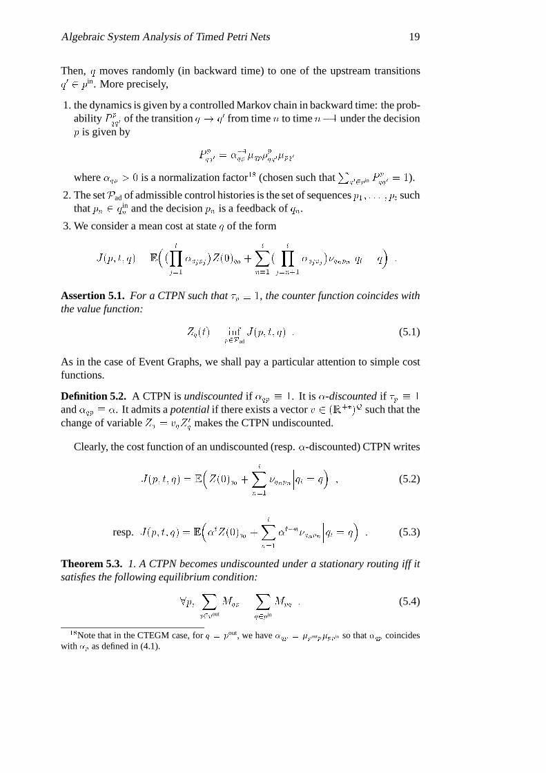
Then, q moves randomly (in backward time) to one of the upstream transitionsq0 2 pin. More precisely,
1. the dynamics is given by a controlled Markov chain in backward time: the prob-ability P p
qq0 of the transition q ! q0 from time n to time n�1 under the decisionp is given by
Pp
qq0 = ��1qp �qp�p
qq0�pq0
where �qp > 0 is a normalization factor18 (chosen such thatP
q02pin Pp
qq0 = 1).
2. The setPad of admissible control histories is the set of sequences p1; : : : ; pt suchthat pn 2 qin
n and the decision pn is a feedback of qn.
3. We consider a mean cost at state q of the form
J(p; t; q) = E
�� tYj=1
�qjpj
�Z(0)q0 +
tXn=1
� tYj=n+1
�qjpj
��qnpn
���qt = q�:
Assertion 5.1. For a CTPN such that �p � 1, the counter function coincides withthe value function:
Zq(t) = infp2Pad
J(p; t; q) : (5.1)
As in the case of Event Graphs, we shall pay a particular attention to simple costfunctions.
Definition 5.2. A CTPN is undiscounted if �qp � 1. It is �-discounted if �p � 1
and �qp � �. It admits a potential if there exists a vector v 2 (R+�)Q such that thechange of variable Zq = vqZ
0q makes the CTPN undiscounted.
Clearly, the cost function of an undiscounted (resp. �-discounted) CTPN writes
J(p; t; q) = E
�Z(0)q0 +
tXn=1
�qnpn
���qt = q�; (5.2)
resp. J(p; t; q) = E
��tZ(0)q0 +
tXn=1
�t�n�qnpn
���qt = q�: (5.3)
Theorem 5.3. 1. A CTPN becomes undiscounted under a stationary routing iff itsatisfies the following equilibrium condition:
8p;Xq2pout
Mqp =Xq2pin
Mpq : (5.4)
18Note that in the CTEGM case, for q = pout, we have �qp = �poutp�ppin so that �qp coincideswith �p as defined in (4.1).

20 G. Cohen, S. Gaubert and J. P. Quadrat
Then, the only origin independent routing policy which makes the net undiscountedis given by19:
8q0 2 pin; �p
qq0 =MqpP
q002pout Mq00p
: (5.5)
2. A CTPN with �p � 1 becomes �-discounted under a stationary routing iff
8p;Xq2pin
Mqp = ��Xq2pout
Mpq
�: (5.6)
3. There exists a stationary routing under potential v iff
8p;Xq2pout
vqMqp =Xq2pin
Mpqvq : (5.7)
4. A CTEGM with routing � admits a potential v iff for all q 2 Q; p 2 qin,
vq =Xq02pin
�qp�p
qq0�pq0vq0 : (5.8)
Proof. We prove item 3 (which contains item 1 as a special case). The CTPN haspotential v iff for all p, the matrix
Pp
qq0 = v�1q M�1qp �
p
qq0Mpq0vq0
is stochastic. Summing up as q0 2 pin, we get vqMqp =P
q02pin �p
qq0Mpq0vq0 . Sum-ming up as q 2 pout and using the fact that the transpose of �p�;� is stochastic, we getthe necessary condition (5.7). Then, the origin independent routing policy
�p
qq0 =vqMqpP
q002pout vq00Mq00p
8q0 2 pin (5.9)
turns out to be admissible, which shows that the condition is also sufficient. Theother points are left to the reader.
5.2 Input-Output Representation of CTPN
Pursuing the program previously illustrated with additive systems (CTEGM), weprovide an algebraic input-output representation for CTPN. In view of the dynam-ics of CTPN (see (3.2)), we introduce (min,+) polynomials and formal series inseveral commutative indeterminates. Given a family of indeterminates fzigi2I(not necessarily finite), we denote by (R+)(I) the set of almost zero sequences
19This is a fairness condition which states that tokens are routed equally to the downstream arcs,counted with their multiplicities.

Algebraic System Analysis of Timed Petri Nets 21
�i 2 R+; i 2 I (such that I(�)
def= fi 2 I j �i 6= 0g is finite). A generalized20
formal series in the commutative indeterminates zi with coefficients in Rmin is asum
s =M
�2(R+)(I)
s�Oi2I(�)
z�i
i ; s� 2 Rmin : (5.10)
It is a polynomial whenever s� = " for all but a finite number of �. The numericalfunction associated with a series s is the map S : RI ! R[ f�1g,
S(z) = inf�
�s� +
Xi2I(�)
�izi
�: (5.11)
When s is a nonzero polynomial, the infimum in (5.11) is finite. This defines aproper notion of finitely valued (min,+) polynomial function. Polynomial functionsare stable by pointwise min, pointwise sum and composition. It is clear that (3.2)is nothing but a polynomial induction of the form
x(t) = A(x(t); : : : ; x(t� �); u(t); : : : ; u(t� � )); (5.12)
y(t) = C(x(t); : : : ; x(t� � ); u(t); : : : ; u(t� � )) ; (5.13)
whereA;C are polynomial functions and �def= maxp �p. Thus, CTPN and (min;+)
recurrent stationary polynomial systems coincide. For simplicity, we shall limitourselves to SISO systems (the MIMO case is not more difficult, although the no-tation is more intricate). We introduce the family of indeterminates u� ; � 2 N. Theseries s given by (5.10) is a Volterra series [11] if for all � , the series is a polyno-mial in the indeterminate u� (equivalently, if the indeterminate u� appears in (5.10)with a finite number of exponents). The evaluation su of the Volterra series s at theinput u is obtained by substituting u(t� � ) for the indeterminate u� .
Theorem 5.4 (Volterra Expansion). The output of an explicit SISO CTPN is ob-tained as the evaluation of a Volterra series:
y(t) = su(t) = inf�
�a� +
X�2I(�)
��u(t� � )�: (5.14)
A case of particular interest arises for inputs with finite past: u(� ) = " for � �T0. Then, for all t, the Volterra expansion of y(t) is obviously finite.
5.3 Behavioral Properties of CTPN
Theorem 5.5. The input-output mapH of a MIMO CTPN is
1. stationary,
20We allow nonnegative real valued exponents �i, not only integer ones.

22 G. Cohen, S. Gaubert and J. P. Quadrat
2. causal,
3. monotone: u � v) Hu � Hv,
4. Scott continuous,
5. concave (see Theorem 4.11 for the definitions).
Undiscounted CTPN satisfy the following property.
6. Homogeneity: H(� + u) = �+H(u).
CTPN with potential v satisfy the following.
7. (vu; vy)-homogeneity: H(�vu + u) = �vy +Hu.
All these properties are immediate consequences of the (MIMO extension) ofthe Volterra expansion (5.14). Again, these properties are accurate: it could beshown that an map satisfying the above properties is a limit of CTPN operators,but we shall not attempt to detail this statement here.
5.4 Asymptotic Properties of Undiscounted Petri Nets
Theorem 5.6. For a strongly connected undiscounted CTPN, we have
limt!1
1
tZq(t) = �; 8q ;
where � is a constant. The periodic throughput � is characterized as the uniquevalue for which a finite vector v is solution of
v = minp
(��p � ��p + P pv) : (5.15)
Indeed, the asymptotic behavior of Z(t) is known in much more details [27].Note that the effective computation of � from (5.15) proceeds from standard algo-rithms (Policy Improvement [28], Linear Programming).
Proof. This is an adaptation of standard stochastic control results [28, Chap. 33,Th. 4.1]. The growth rate � is independent of the initial point q for the subclass ofcommunicating systems21. This assumption is equivalent to the strong connectivityof the net.
There is an equivalent characterization of � which exhibits the analogy with theCTEG case in a better way. A feedback policy (or policy22, for short) is a map u :
Q! P . The policy is admissible if u(q) 2 qin, that is, if setting pn = u(qn) yields
21The system is communicating if for all q; q0, there is a policy u and an integer k such that(Pu
qq0)k > 0 —i.e. q has access to q0.
22This feedback policy has nothing to do with the routing policy introduced in x3.

Algebraic System Analysis of Timed Petri Nets 23
and admissible policy for the stochastic control problem presented in x5.1. With apolicy u are associated the following vectors and matrices
�uqdef= �qu(q) ; �uq
def= �u(q) ; P u
qq0def= P
u(q)
qq0 :
We denote by R(u) the set of final classes23 of the matrix P u. For each class r 2R(u), we have a unique invariant measure �ru with support r (i.e. �ruP u = �ru,and �ru
q = 0 if q 62 r.)
Theorem 5.7. For a strongly connected undiscounted CTPN, we have
� = minu
minr2R(u)
�ru�u
�ru�u: (5.16)
Thus, � is the minimal ratio of the mean marking over the mean holding time inthe places visited following a stationary policy. In the CTEG case, the final classesare precisely circuits and the invariant measures are uniform on the final classes,so that (5.16) reduces to the well known (4.22).
The proof of Theorem 5.7 uses the fact that the rate� is obtained asymptoticallyfor stationary policies, together with the following lemma.
Lemma 5.8. Let u denote a policy such that P u admits a positive invariant mea-sure �. The unique � such that there exists a finite vector v:
v = �u � ��u + P uv (5.17)
is given by
� =��u
��u: (5.18)
Proof. Left multiplying (5.17) by the row vector �, we get that � is necessarilyequal to (5.18). Conversely, we are reduced to prove the existence of a solution(�; v) whenP u is irreducible. Then 1 is a simple eigenvalue ofP u, hence, Im(P u�
I) is jQj�1 dimensional. Moreover, �u 62 Im(P u�I) (for �u = P uv�v) ��u =
�(P uv � v) = 0, a contradiction). Hence, R�u+ Im(P u � I) = RQ.
It is not surprising that the terms at the right-hand side of (5.16) are indeed invari-ants of the net.
Theorem 5.9 (Invariants). Given an undiscounted CTPN, for all policy u and forall final class r associated with u,
Iurdef= �ur�u =
Xq2r
�ur�uq (5.19)
is invariant by firing of transitions.
23The classes of a matrix A are by definition the strongly connected components of the graph ofA. A class is final if there is no other class downstream.

24 G. Cohen, S. Gaubert and J. P. Quadrat
Proof. After firing once transition q 2 r (the case when q 62 r is trivial), Iur in-creases by
��urq +
Xq02(qout)out\r
�urq0 P
uq0q
which is zero because �ur is an invariant measure of P u with support r.
Example 5.10. The CTPN shown in Fig. 2a is equivalent to that of Fig. 2d un-der a fair routing policy independent of the origin of the tokens. In this particularcase, we obtain the same periodic throughput � as in the case of the bijective rout-ing shown in Fig. 2c (see (4.30)). This can be seen from the following table andFormula (5.16).
Policy Final classes Invariant measures Invariantsu1(q3) = p1u1(q4) = p2
r1 = fq1; q3g,r2 = fq2; q4g
�u1r1 = [12; 0; 1
2; 0]
�u1r2 = [0; 12; 0; 1
2]
Iu1r1 =12(mp1 +mp3 )
Iu1r2 =12(mp2 +mp4 )
u2(q3) = p1u2(q4) = p5
r1 �u1r1 Iu1r1
u3(q3) = p5u3(q4) = p2
r2 �u1r2 Iu1r2
u4(q3) = p5u4(q4) = p5
r3 = fq1; q2; q3; q4g�u4r3 = [
14; 14; 14; 14] Iu4r3 =
14(mp3 +mp2 +mp5 )
Finally, we indicate how the above results can be extended to CTPN with potential.With a feedback policy u we associate the matrix Ru: Ru
qq0 = �qu(q)�u(q)
qq0 �u(q)q0 ifq0 2 u(q)in (Ru
qq0 = 0 otherwise); we denote byR(u) the set of final classes of Ru;which each final class r we associate a left eigenvector of Ru: �ru = �ruRu withsupport r; and we define �u; �u as in Theorem 5.7. We denote by diag v the diagonalmatrix with diagonal entries (diag v)qq = vq. Then, the folllowing formula is animmediate consequence of Theorem 5.7.
Corollary 5.11. For a strongly connected CTPN with potential v, we have
limt!1
1
tZq(t) = �q; where v�1q �q = min
umin
r2R(u)
�ru�u
�ru(diag v)�u: (5.20)
The terms �ru�u which determine the throughput are of course invariants of thenet. More generally, it follows from standard dynamic programming results thatthe counter functions of �-discounted CTPN exhibit a geometric growth (or con-vergence) with rate �. The geometric growth of other classes of CTPN could beobtained by transferring existing results about non normalized dynamic program-ming inductions [29].
References
[1] F. Baccelli, G. Cohen, and B. Gaujal. Recursive equations and basic properties oftimed Petri nets. J. of Discrete Event Dynamic Systems, 1(4):415–439, 1992.

Algebraic System Analysis of Timed Petri Nets 25
[2] F. Baccelli, G. Cohen, G.J. Olsder, and J.P. Quadrat. Synchronization and Linearity.Wiley, 1992.
[3] F. Baccelli, S. Foss, and B. Gaujal. Structural, temporal and stochastic properties ofunbounded free-choice petri nets. Rapport de recherche, INRIA, 1994.
[4] J. Berstel and C. Reutenauer. Rational Series and their Languages. Springer, 1988.[5] H. Braker. Algorithmsand Applicationsin Timed Discrete Event Systems. PhD thesis,
Delft University of Technology, Dec 1993.[6] H. Braker and J. Resing. Periodicity and critical circuits in a generalized max-algebra
setting. Discrete Event Dynamic Systems. toappear.[7] P. Chretienne. Les Reseaux de Petri Temporises. These Universite Pierre et Marie
Curie (Paris VI), Paris, 1983.[8] G. Cohen, D. Dubois, J.P. Quadrat, and M. Viot. Analyse du comportement peri-
odique des systemes de production par la theorie des dioıdes. Rapport de recherche191, INRIA, Le Chesnay, France, 1983.
[9] G. Cohen, P. Moller, J.P. Quadrat, and M. Viot. Algebraic tools for the performanceevaluation of discrete event systems. IEEE Proceedings: Special issue on DiscreteEvent Systems, 77(1), Jan. 1989.
[10] P. Dudnikov and S. Samborskiı. Endomorphisms of finitely generated free semimod-ules. In V. Maslov and S. Samborskiı, editors, Idempotent analysis, volume 13 of Adv.in Sov. Math. AMS, RI, 1992.
[11] E.Sontag. Polynomial response maps. Lecture notes in control and information sci-ences. Springer, 1979.
[12] S. Gaubert. Theorie des systemes lineaires dans les dioıdes. These, Ecole des Minesde Paris, July 1992.
[13] S. Gaubert. Rational series over dioids and discrete event systems. In Proc. of the11th Conf. on Anal. and Opt. of Systems: Discrete Event Systems, number 199 in Lect.Notes. in Control and Inf. Sci, Sophia Antipolis, June 1994. Springer.
[14] S. Gaubert. Resource optimization and (min,+) spectral theory. IEEE-TAC, 1995, toappear.
[15] S. Gaubert. Rational series over the (max,+) semiring, discrete event systems andBellman processes. in preparation, 1995.
[16] G. Gierz, K.H. Hofmann, K. Keimel, J.D Lawson, M. Mislove, and D.S. Scott. ACompendium of Continuous Lattices. Springer, 1980.
[17] M. Gondran and M. Minoux. Graphes et algorithmes. Eyrolles, Paris, 1979. Engl.transl. Graphs and Algorithms, Wiley, 1984.
[18] H.P. Hillion and J.M. Proth. Performance evaluation of job-shop systems using timedevent-graphs. IEEE Trans. on Automatic Control, 34(1):3–9, Jan 1989.
[19] D. Krob. Quelques exemples de series formelles utilisees en algebre non commuta-tive. Rapport de recherche 90-2, Universite de Paris 7, LITP, Jan. 1990.
[20] D. Krob and A. Bonnier-Rigny. A complete system of identities for one letter rationalexpressions with multiplicities in the tropical semiring. Rapport de recherche 93.07,Universite de Paris 7, LITP, 1993.
[21] S. Laftit, J.M. Proth, and X.L. Xie. Optimization of invariant criteria for event graphs.IEEE Trans. on Automatic Control, 37(6):547–555, 1992.
[22] P. Moller. Theorie algebrique des Systemes a Evenements Discrets. These, Ecole desMines de Paris, 1988.
[23] A. Munier. Regime asymptotique optimal d’un graphe d’evenements temporise

26 G. Cohen, S. Gaubert and J. P. Quadrat
generalise: application a un probleme d’assemblage. APII, 27(5):487–513, 1993.[24] M. Plus. A linear system theory for systems subject to synchronization and saturation
constraints. In Proceedings of the first European Control Conference, Grenoble, July1991.
[25] I.V. Romanovskiı. Optimization and stationary control of discrete deterministic pro-cess in dynamic programming. Kibernetika, 2:66–78, 1967. Engl. transl. in Cyber-netics 3 (1967).
[26] L.H. Rowen. Polynomials identities in Ring theory. Academic Press, 1980.[27] P.J. Schweitzer and A. Federgruen. Geometric convergence of value-iteration in mul-
tichain Markov decision problems. Adv. Appl. Prob., 11:188–217, 1979.[28] P. Whittle. Optimization over Time, volume II. Wiley, 1986.[29] W.H.M. Zijm. Generalized eigenvectors and sets of nonnegative matrices. Lin. Alg.
and Appl., 59:91–113, 1984.