Algebraic Tools for the PerformanceEvaluation of Discrete Event Systems∗

Guy COHEN†

Centre d’Automatique et Informatique, Ecole des Mines de Paris,35 Rue Saint-Honore — 77305 Fontainebleau Cedex, France‡

Pierre MOLLERRhone-Poulenc, Lyon, France§

Jean-Pierre QUADRATINRIA, Le Chesnay, France

Michel VIOTEcole Polytechnique, Palaiseau, France

AbstractIn this paper, it is shown that a certain class of Petri nets called event

graphs can be represented as linear ”time-invariant” finite-dimensional sys-tems using some particular algebras. This sets the ground on which a theoryof these systems can be developped in a manner which is very analogous tothat of conventional linear system theory. Part 2 of the paper is devotedto showing some preliminary basic developments in that direction. Indeed,there are several ways in which one can consider event graphs as linear sys-tems: these ways correspond to approaches in the time domain, in the eventdomain and in a two-dimensional domain. In each of these approaches, adifferent algebra has to be used for models to remain linear. However, thecommon feature of these algebras is that they all fall into the axiomaticdefinition of ”dioids”. Therefore, Part 1 of the paper is devoted to a unifiedpresentation of basic algebraic results on dioids.

1 Introduction

Definitions and examples of Discrete Event Dynamic Systems (DEDS) will cer-tainly be found elsewhere in this special issue. But there are several aspects ofDEDS on which to focuss one’s attention. In this work, we are interested inanswering such questions as:∗IEEE Proceedings, Vol. 77, pp. 39–58, 1989†Also with INRIA.‡This is the address for correspondence.§On leave from IIASA, Laxenburg, Austria.

1

• how many events of a particular type will occur in a certain time interval?

• at which time the nth occurrence of an event of a certain type willhappen?. . .

This is what is usually meant by “performance evaluation”. Apart from dis-crete event computer simulation which probably remains the most widespreadpractice, performance evaluation is also the scope of queueing theory [11] andtimed Petri nets [17]. Whereas the former involves a stochastic framework andis devoted to average long-term evaluation, the latter is rather deterministic andit can deal with transient behaviour.

Our approach is also deterministic although there has been already someattempt to extend it to stochastic situations [19, 15]. If one considers a manu-facturing workshop for example, it may be argued that, on the short term, theprobability of machine breakdown is very low (hopefully!), whereas the servicetimes experienced by parts at all machines are likely to be deterministic (timeto drill a hole into a piece of iron, . . . ). The same holds true in such contextsas performance evaluation of dedicated chips in signal processing. . . However,it is not in our intention to claim that a purely deterministic modelling of suchsystems is uniformely realistic. The claim is that this deterministic approachmay sometimes be more adequate than assuming exponential service times forexample. If one is ready to admit this statement (so that our theory mighthave a nonempty field of application), we believe that it is reasonable to starta theory of DEDS with the simplest situation.

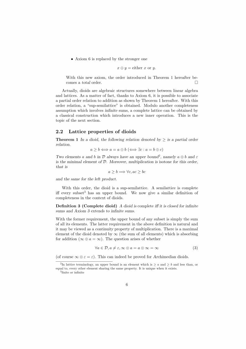
Apart from determinism, simplicity also means linearity. Linearity is a mostwelcome property when it holds true. The major message in this paper is that,for a certain class of DEDS, namely those also modelled by event graphs (aspecial class of Petri nets — see Figure 1 hereafter), linearity appears to bean intrinsic property, provided that one accepts the idea of getting familiarwith new algebraic tools. These algebraic structures, that we call dioids afterGondran and Minoux [9], present some interesting similarities with our familiarlinear algebra, vector spaces, etc. . . Of course, there are also important differ-ences. But it is striking to see how many features and concepts of conventionallinear system theory naturally extend to event graphs. Of course, the practi-cal or intuitive meaning of these concepts should be adapted to the nature ofapplications covered by DEDS, but the algebraic similarity often goes very far.

This paper comes after several other papers on the same topic. In the ear-liest approach [3], a state space representation was introduced using variablesinterpreted as dates (later on called daters) which were indexed by event num-bers (integers). The dioid (R∪{−∞},max,+) [7] (or (Z∪{−∞},max,+) if oneprefers to deal with integer, rather than real, dates) was the appropriate alge-braic tool for this event domain representation. Then, in [4], the correspondinginput-ouput representation, or transfer matrix, was proposed using formal poly-nomials and series with coefficients in the above dioid. Finally, in [6], it wasbriefly shown that another state space representation could be obtained using

2

y

u u

x x

x

1

1

2

2

3

Initial markingof a place(token)

Holding timeof tokens in a

place(in time units)

.

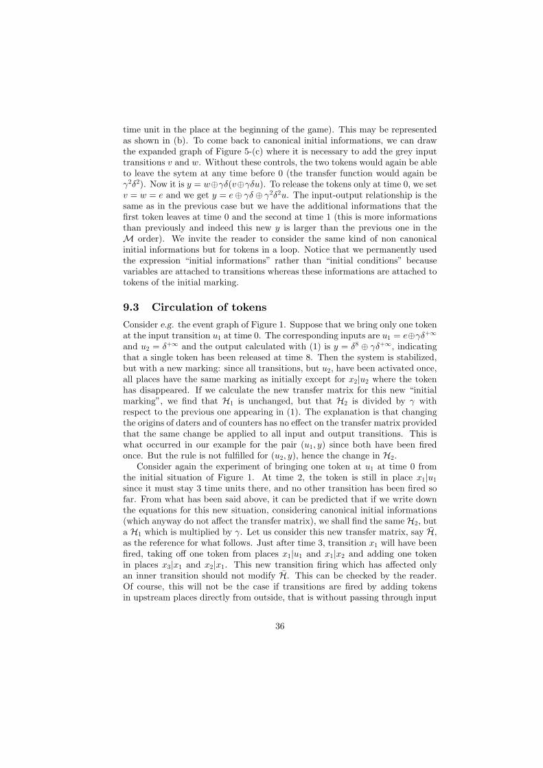
variables indexed by (discrete) time (this is the usual time domain representa-tion), those variables being interpreted as numbers of events (they were thuscalled counters). But for this new model to remain linear, it was necessary toappeal to another dioid, namely (Z ∪ {+∞},min,+). Again a correspondinginput-output representation could also be proposed. But we found that thebest representation was an input-output representation, in a two-dimensionaldomain using series in two formal variables (the backward shift operators indating, say δ, and in counting, say γ) with boolean coefficients. This gave birthto yet another dioid which will be discussed hereafter. For the event graph ofFigure 1, the following representation is obtained

y = H1u1 +H2u2 = δ8(γδ2)∗u1 + γδ5(γδ2)∗u2 (1)

The reader is referred to the second part of this paper to understand the meaningof this expression.

Figure 1: An event graph

From these considerations we draw the following conclusion: event graphs arelinear systems on various dioids; therefore, there is an incentive to study thesealgebraic structures in the most general manner, avoiding the use of propertiesor axioms which are too specific of one particular dioid and which are not likelyto carry over other modelling approaches. It is one objective of this paper topresent such an abstract study in a sufficiently self-contained way, so as to serveas a possible basis for further work in this direction. This does not mean that

3

all the results presented in the first part of this paper are original: a few of themappear here for the first time, as far as we know, but most of them can be foundscattered in the literature on dioids (see [9, 7] and references therein), latticetheory and lattice-ordered semigroups [8], and probably in other fields we arenot even aware of. It is a difficulty of this emerging theory of (some) DEDS tohave to appeal to mathematical tools which are not as familiar to engineers asconventional linear algebra.

The second part of the paper will be devoted to discussing the various mod-elling approaches of DEDS alluded to hereabove, to summarizing the earlierdevelopments on elements of system theory and to discussing their practicalsignificance. The reader should wait until this second part for finding moreconcrete applications of the tools and results abstractly introduced in the firstpart (or he may first scan the second part before comming back to the first). Ina conclusion, we try to discuss open problems and directions of future researchfor this emerging theory.

Part I

Dioid theory

2 Axiomatic definition and basic properties

2.1 Dioid definition

Definition 1 A set D supplied with two inner operations denoted by ⊕ and⊗ (called “sum” or “addition”, and “product” or “multiplication”) is a dioid ifthe following axioms are fulfilled:

Axiom 1 (Associativity)

∀a, b, c ∈ D, (a⊕ b)⊕ c = a⊕ (b⊕ c) and (a⊗ b)⊗ c = a⊗ (b⊗ c)

Axiom 2 (Commutativity of addition)

∀a, b ∈ D, a⊕ b = b⊕ a

Axiom 3 (Distributivity)

∀a, b, c ∈ D, (a⊕ b)⊗ c = (a⊗ c)⊕ (b⊗ c)

This is right distributivity of product over sum. Since commutativity of productis not a priori required, we do require left distributivity too.

Axiom 4 (Null and identity elements)

∃ε ∈ D : ∀a ∈ D, a⊕ ε = a

4

∃e ∈ D : ∀a ∈ D, a⊗ e = e⊗ a = a

Axiom 5 (Absorbing null element)

∀a ∈ D, a⊗ ε = ε⊗ a = ε

Axiom 6 (Idempotency of addition)

∀a ∈ D, a⊕ a = a

¤

Definition 2 (Commutative dioid) A dioid is commutative iff multiplica-tion is commutative.

Notice In the sequel of this paper, the sign ⊗ will be most of the time omitted(or replaced by a dot) as it is usual in conventional algebra.

Comments

(i) Some of the results hereafter do not depend on Axiom 5 but this axiomseems to be necessary when moving from “scalar” to “matrix” dioids aswe shall see later on.

(ii) Axiom 6 prevents addition from being cancellative1 unless the dioid re-duces to ε (a ⊕ a = a ⊕ ε would imply a = ε). Thus dioids cannot beembedded into rings. Following Gondran and Minoux [9], we leave theterminology “semiring” sometimes encountered in the literature for thecancellative case.

(iii) Our definition of a dioid is somewhat less general than that of Gondranand Minoux who require the following weaker substitute for Axiom 6

a = b⊕ c and b = a⊕ d =⇒ a = b (2)

which would be sufficient for stating Theorem 1 hereafter. In fact, alldioids encountered in the second part of this paper satisfy Axiom 6. Anexample of a dioid satisfying (2) but not Axiom 6 is (R+,+,×). Howeverthis again corresponds to a cancellative addition and it is natural to embedthis dioid in (R,+,×), that is in our usual algebra.

(iv) Helbig [10], who himself refers to Zimmermann (see references therein),defines an extremal algebra with axioms which are very close but strongerthan ours on two points:

• product is commutative;1Cancellative means that a⊕ b = a⊕ c⇒ b = c.

5

• Axiom 6 is replaced by the stronger one

x⊕ y = either x or y.

With this new axiom, the order introduced in Theorem 1 hereafter be-comes a total order. ¤

Actually, dioids are algebraic structures somewhere between linear algebraand lattices. As a matter of fact, thanks to Axiom 6, it is possible to associatea partial order relation to addition as shown by Theorem 1 hereafter. With thisorder relation, a “sup-semilattice” is obtained. Modulo another completenessassumption which involves infinite sums, a complete lattice can be obtained bya classical construction which introduces a new inner operation. This is thetopic of the next section.

2.2 Lattice properties of dioids

Theorem 1 In a dioid, the following relation denoted by ≥ is a partial orderrelation.

a ≥ b⇐⇒ a = a⊕ b (⇐⇒ ∃c : a = b⊕ c)Two elements a and b in D always have an upper bound2, namely a ⊕ b and εis the minimal element of D. Moreover, multiplication is isotone for this order,that is

a ≥ b =⇒ ∀c, ac ≥ bcand the same for the left product.

With this order, the dioid is a sup-semilattice. A semilattice is completeiff every subset3 has an upper bound. We now give a similar definition ofcompleteness in the context of dioids.

Definition 3 (Complete dioid) A dioid is complete iff it is closed for infinitesums and Axiom 3 extends to infinite sums.

With the former requirement, the upper bound of any subset is simply the sumof all its elements. The latter requirement in the above definition is natural andit may be viewed as a continuity property of multiplication. There is a maximalelement of the dioid denoted by ∞ (the sum of all elements) which is absorbingfor addition (∞⊕ a =∞). The question arises of whether

∀a ∈ D, a 6= ε,∞⊗ a = a⊗∞ =∞ (3)

(of course ∞⊗ ε = ε). This can indeed be proved for Archimedian dioids.2In lattice terminology, an upper bound is an element which is ≥ a and ≥ b and less than, or

equal to, every other element sharing the same property. It is unique when it exists.3finite or infinite

6

Definition 4 (Archimedian dioid) A dioid is Archimedian iff the followingholds true

∀a, b ∈ D,∃c and d ∈ D : ac ≥ b and da ≥ b

Theorem 2 In a complete Archimedian dioid, (3) holds true.

Proof We give the proof for right multiplication by ∞. From Definition 4,given a, for all b, there exists cb such that acb ≥ b. One has that

a∞ = a(⊕x∈D

x) ≥ a(⊕b∈D

cb) =⊕b∈D

acb ≥⊕b∈D

b =∞

¤A complete dioid being a complete sup-semilattice, and since there is also

a minimal element ε, a new inner operation denoted by ∧, the lower bound4,can be constructed so that the semilattice becomes a complete lattice. This isa classical construction [8, pp. 175–176]. We briefly recall it. For every subsetC of D, we consider the set

E := {x ∈ D | x ≤ y,∀y ∈ C}

which is nonempty since it contains at least ε. The lower bound of C, say z,is defined as the upper bound of E which exists by assumption. Note that zbelongs to E . As a matter of fact, E is bounded from above by all y ∈ C.Since z is less than, or equal to, every element greater than E (by definition),z ≤ y,∀y ∈ C q.e.d.

If C = {a, b, c, . . .}, z is denoted by a ∧ b ∧ c ∧ . . . In general, we use thenotation

∧x∈C x. This operation ∧ is also associative, commutative, idempotent

and has ∞ as “null” element (∞ ∧ a = a,∀a). The following property, calledabsorption law, holds true [8, p. 184]

∀a, b ∈ D, a ∧ (a⊕ b) = a⊕ (a ∧ b) = a (4)

Remark 1 One has the following equivalences

a ≥ b⇐⇒ a = a⊕ b⇐⇒ b = a ∧ b

However, this symmetry involves the lattice properties only. From the dioidpoint of view, one should remember that multiplication is isotone in particularbecause of Axiom 3. But distributivity will not hold true in general for mul-tiplication over ∧ as one can check for the dioid M introduced in the secondpart of this paper. This nonsymmetry is recalled by the notations: + and ×are circled whereas ∧ is not. Nevertheless, since multiplication is isotone, it iseasy to check that

(a ∧ b)c ≤ (ac) ∧ (bc) (5)

and the same for left multiplication. ¤4obeying the dual definition of the upper bound — see footnote 2

7

Notice that ∧ does not necessarily distribute over ⊕ or conversely. We canhowever state that

∀a, b, c ∈ D, (a ∧ b)⊕ c ≤ (a⊕ c) ∧ (b⊕ c) (6)(a⊕ b) ∧ c ≥ (a ∧ c)⊕ (b ∧ c) (7)

A lattice is distributive when equality holds true in (6)–(7). Indeed, equality ineither (6) or (7) implies the other equality too [8, p. 188]. The following twotheorems can also be found in [8, pp. 207 and 212 respectively].

Theorem 3 A necessary and sufficient condition for a lattice to be distributiveis that

a ∧ c = b ∧ ca⊕ c = b⊕ c

}=⇒ a = b

Theorem 4 Every multiplicative group G supplied with an order relation suchthat multiplication is isotone and G is a sup-semilattice is a reticulated groupand a distributive lattice.

“Reticulated group” means in particular that multiplication distributes overboth the upper and the lower bounds (in our case, over ⊕ and ∧). Hence, inthis situation, all desirable properties hold true simultaneously. However, theassumption that a dioid is a multiplicative group is rather strong and it will nothold true for the dioid M considered in the second part.

Definition 5 (Distributive dioid) A dioid D is distributive iff it is completeand

∀C ⊂ D, ∀a ∈ D, (∧c∈Cc)⊕ a =

∧c∈C

(c⊕ a) (8)

(⊕c∈C

c) ∧ a =⊕c∈C

(c ∧ a) (9)

Notice that here distributivity is required to extend to infinite subsets too.Moreover, both properties should be required now since one does not imply theother [8, p. 189].

2.3 Matrix dioids

Starting from a “scalar” dioid D, consider square n × n matrices with entriesin D. Sum and product of matrices are defined conventionally after the sumand product of scalars in D. The set of n× n matrices supplied with these twooperations is also a dioid which is denoted by Dn×n. The only point that deservessome attention is the existence of an identity element. Thanks to Axiom 5, theusual identity matrix with entries equal to e on the diagonal and to ε elsewhereis the identity element of Dn×n. This identity matrix will also be denoted by e

8

and it will be clear from the context which e is meant. In the same way, thenull n× n matrix is denoted by ε.

Notice that if D is a commutative dioid, this will not be the case for Dn×n ingeneral. In the same way, if D is Archimedian, Dn×n will not be so in general.But since addition of matrices simply involves the addition of similar entries, itis clear that Dn×n is complete (respectively distributive) whenever D is so. AlsoA ≥ B ⇐⇒ {aij ≥ bij , i = 1, . . . , n, j = 1, . . . , n} and (A ∧B)ij = aij ∧ bij .

It is sometimes useful to think of A ∈ Dn×n as representative of a graphwith n nodes and with a directed arc from node i to node j weighted by Aji ifthis entry of A is different from ε, and with no arc otherwise. The product (inD) of the weights of arcs composing a path or a circuit is called weight of thispath or circuit. The number of arcs is called the length of the path or circuit.The entry (j, i) of some power Ap of A indicates the maximal weight over allpaths of length equal to p and going from i to j. “Maximal” of course refers tothe upper bound of the weights of these paths for the order of D. It is worthnoticing that this interpretation holds true because non existing arcs received aweight equal to ε, so that paths that would make use of this non existing arcsare also weighted by ε thanks to Axiom 5, and thus they cannot be maximal.

3 Linear equations in complete dioids

The most general linear equation in a dioid is

ax⊕ b = cx⊕ d (10)

where a, b, c, d ∈ D or Dn×n and x is the unknown in the same dioid. Throughoutthis section, D is supposed to be a complete dioid. Hereafter, we only considerparticular subclasses of this general equation which will prove useful in thesecond part of this paper.

3.1 The equation ax⊕ b = c and residuation

In D (or Dn×n), we first consider the equation in x

ax⊕ b = c (11)

This equation does not always admit a solution but it may also have several oran infinity of solutions. This may as well happen in usual linear algebra when,for example, a is a non invertible matrix. Pseudo-inverses are then considered.Here, a first obvious necessary condition for existence is that b ≤ c. It is metin particular if b = ε. Even in this case, existence and uniqueness are notguaranteed. In order to recover existence and uniqueness when b ≤ c, we shallmodify the concept of “solution” to (11) and we shall retain that of “greatestsubsolution”.

9

Definition 6 A subsolution of (11) is an x such that ax⊕ b ≤ c.

Theorem 5 The set of subsolutions of (11), say S, is not empty iff b ≤ c. Thenthe upper bound of S belongs to S and it is also the greatest subsolution of

ax = c (12)

Proof The condition b ≤ c is an immediate consequence of (11) and Theorem1. Conversely, if it is satisfied, then S contains at least ε thanks to Axiom 5.Let z be the upper bound of S. The following proves that z belongs to S

az = a(⊕y∈S

y) =⊕y∈S

ay ≤ c

Finally, we prove that S is identical to S′ which is defined as the set of subsolu-tions of (12). On the one hand, y ∈ S ⇒ ay⊕ b ≤ c⇒ ay ≤ c⇒ y ∈ S′. On theother hand, y ∈ S′ ⇒ ay ≤ c ⇒ ay ⊕ b ≤ b ⊕ c = c since {b ≤ c ⇔ c = c ⊕ b}.Hence y ∈ S. ¤

From now on, we thus limit ourselves to the study of equation (12).

Definition 7 (Residuation) The (left) residue of c by a, denoted by a\c, isdefined as the greatest subsolution of (12).

The terminology comes from lattice-ordered semigroups (see [8, pp. 220]).

Remark 2 Since we do not assume that D is commutative, it is possible toconsider equations of the form xa = c and the corresponding right pseudo-inverse solution would be denoted by c/a.

Remark 3 It should be kept in mind that one cannot in general associate aparticular element of D (supposedly denoted by a[) to the mapping c 7→ a\c, insuch a way that a\c = a[ ⊗ c, for the reason that that mapping is not “linear”in D as we are going to see it in the study of the new operation \.

Theorem 6 If (12) has a true solution, then a\c is also a solution and it is thegreatest one.

The proof is straightforward. As a corollary, if a−1 exists, then the solution isunique and a\c = a−1c.

Theorem 7 The expression a\b is nonincreasing as a function of a and nonde-creasing as a function of b. Moreover the following inequalities and equalitieshold true

a(a\b) ≤ b (13)

(a\a) ≥ e (14)

10

a(a\a) = a (15)

e\a = a (16)

ε\a =∞ (17)

(a\b)c ≤ a\(bc) (18)

a\(b\c) = (ba)\c (19)

(a\b)⊕ (a\c) ≤ a\(b⊕ c) (20)

(a\b) ∧ (c\b) = (a⊕ c)\b (21)

(a\b) ∧ (a\c) = a\(b ∧ c) (22)

(a\b)⊕ (c\b) ≤ (a ∧ c)\b (23)

Proof Most of the inequalities and of some equalities are readily derived fromthe very definition of residuation. We only give a proof for the non obviousequalities. For (15), two opposite inequalities are derived from (13) and (14).

For (19), let x = b\c, y = a\x, z = (ba)\c. On the one hand, {bx ≤c and ay ≤ x} ⇒ {bay ≤ bx ≤ c} ⇒ {y ≤ z}. On the other hand,{baz ≤ c} ⇒ {az ≤ x} ⇒ {z ≤ y}.

For (21), let x = (a⊕ c)\b, y = a\b, z = c\b. On the one hand, {(a⊕ c)x ≤b} ⇒ {ax ≤ b and cx ≤ b} ⇒ {x ≤ y and x ≤ z} ⇒ {x ≤ y ∧ z}. On the otherhand, {ay ≤ b and cz ≤ b} ⇒ {a(y∧z) ≤ b and c(y∧z) ≤ b} ⇒ {(a⊕c)(y∧z) ≤b} ⇒ {y ∧ z ≤ x}.

For (22), let x = a\b, y = a\c, z = a\(b ∧ c). On the one hand, {ax ≤b and ay ≤ c} ⇒ {a(x ∧ y) ≤ ax ∧ ay ≤ b ∧ c} ⇒ {x ∧ y ≤ z}. On the otherhand, {az ≤ b∧c} ⇒ {az ≤ b and az ≤ c} ⇒ {z ≤ x and z ≤ y} ⇒ {z ≤ x∧y}.¤

Comments (15) is a familiar equality for pseudo-inverses; (16) says that e isa neutral element for residuation; (18) and (20) shows that a\b is not a linearfunction of b; (22) means that \ is distributive over ∧. When a−1 and b−1 exist,an interesting consequence of (21) is the formula5

(a⊕ b)\e = a−1 ∧ b−1 (24)

In a (complete) commutative dioid, again with (21), one has that

(ab)/(a⊕ b) = (a⊕ b)\(ab) = (a\(ab)) ∧ (b\(ba))≥ ((a\a)b) ∧ ((b\b)a) from (18)≥ b ∧ a from (14)

but obviously equalities hold throughout when a−1 and b−1 exist. ¤5Recall that −max(a, b) = min(−a,−b).

11

3.2 Matrix residuation

Till now, all that have been said about residuation applies to a complete “scalar”dioid D or to a “matrix” dioid Dn×n. The following theorem relates the residueof B ∈ Dn×n by A ∈ Dn×n (also denoted by A\B) to the scalar residuation.

Theorem 8 Let A,B ∈ Dn×n, then

A\B = AT ¯B (25)

where AT denotes the transpose of A and ¯ is a new matrix product where theoperations ⊕ and ⊗ of D are replaced respectively by ∧ and \ of D (recall that\ distributes over ∧ from (22)).

Proof We consider n = 2 without loss of generality. Moreover, it is obviousthat each pair of corresponding columns of X = A\B and B can be consideredindependently of other pairs. For example, the first column X.1 must satisfy

A11X11 ⊕A12X21 ≤ B11 (26)A21X11 ⊕A22X21 ≤ B21 (27)

which implies

A11X11 ≤ B11 and A21X11 ≤ B21

A12X21 ≤ B11 and A22X21 ≤ B21

or

X11 ≤ Y11 := (A11\B11) ∧ (A21\B21)X21 ≤ Y21 := (A12\B11) ∧ (A22\B21)

On the other hand, Y11 and Y21 also verify (26)-(27), which means that indeedY.1 = X.1 by definition of X. Let us check this for (26) for example

A11[(A11\B11) ∧ (A21\B21)]⊕A12[(A12\B11) ∧ (A22\B21)] ≤ A11(A11\B11)⊕A12(A12\B11)≤ B11 from (13)

This completes the proof. ¤

This theorem extends a result provided by Cuninghame-Green [7] in the contextof the dioid (R ∪ {−∞,+∞},max,+) (where ∧ = min).

3.3 A particular transformation

We now come back to an arbitrary (complete) dioid D and we show an inter-esting transformation which, in some situation, reduces residuation to multipli-cation. An application of this will be encountered in the second part of this

12

paper. Let ϕ be an arbitrary but fixed element in D and let us consider thetransformation

∀a ∈ D, a := a\ϕ (28)

Notice that a⊕ b = a ∧ b from (21) which shows that this transformation isan homomorphism from the sup-semilattice (D,⊕) to the inf-semilattice (D,∧).As a direct consequence of (19) and (28), we also have that

∀a, b ∈ D, ba = a\b (29)

Let us interpret x as a way of “coding” x. We see that, if we have to perform theleft residuation of the “coded” b by a, we can rather multiply b itself by a to theright and then code the result. Of course, the process of coding itself involvesresiduation, but it may be quite simple for elements (at the “denominator”)with can be written as a sum of invertible elements thanks to (21) (this is whathappen in the second part of this paper). However, even in this case, this doesnot mean that we can always replace residuation by product since there may bea problem with “decoding”: the transformation is not a bijection in general.

Everything above applies as well to a matrix dioid Dn×n. Let us howeverdiscuss the relationship between scalar and matrix coding. If a scalar codinghas been defined by some ϕ, we define the n× n matrix

Φ =

ϕ ∞ . . . ∞∞ ϕ

......

. . ....

∞ . . . . . . ϕ

(30)

and we define X as X\Φ. Using (25), it is easy to check that (say, for n = 2)

X =(a bc d

)=⇒ X =

(a c

b d

)where of course e.g. b corresponds to scalar coding of b with ϕ. Notice thetransposition in the formula above: coding a column vector amounts to codingits entries and transposing, the result being a row vector.

Finally, as a consequence of (25) and (29), we have that

BA = A\B = AT ¯ B

3.4 The equation x = ax⊕ b and the “star” operation

We consider the following implicit equation in x

x = ax⊕ b (31)

13

Leta∗ := e⊕ a⊕ a2 ⊕ · · · (32)

Interesting, and easy to check, properties of this star operation are

(a∗)p = a∗,∀p ∈ N and (a∗)∗ = a∗ (33)

Let also a+ := a⊗ a∗ and notice that

a∗ = e⊕ a+ and a∗ ≥ a+ (34)

Theorem 9

(i) a∗b is the least solution of (31).

(ii) For all solution x, one has that x = a∗x.

Proof

(i) Clearly, if x is a solution, x ≥ b and x ≥ ax. On the one hand, apx ≥apb. On the other hand, x ≥ ax ≥ . . . ≥ apx. Hence, x ≥ apb, thusx ≥

⊕∞p=0 a

pb = a∗b. Finally, it is straightforward to check that a∗b is alsoa solution.

(ii) From (31), one gets that x = a(ax⊕ b)⊕ b = . . . = apx⊕ (e⊕ · · · ⊕ ap−1)bfor all p. Summing up all these equalities for p ∈ N yields x = a∗x⊕ a∗b.But from (i) above, a∗x ≥ a∗b or a∗x ⊕ a∗b = a∗x which completes theproof. ¤

Theorem 9 answers the issue of existence of solutions to (31) in complete dioids.About uniqueness, we observe that if the homogeneous equation

x = ax (35)

has a solution y 6= ε, yz is also a solution of (35), ∀z ∈ D, and obviously a∗b⊕yzis a solution of the nonhomogeneous equation (31). In usual linear algebra, it iswell known that all solutions of the nonhomogeneous equation are obtained byadding all solutions of the homogeneous equation to a particular solution of thenonhomogeneous. Here, for such a result to hold true, the “particular solution”has to be the least one (namely a∗b) because “adding” also means “increasing”.

Theorem 10 Let D be a distributive dioid. Then, if x is a solution of (31), itcan be written as x = y ⊕ a∗b where y is a solution of (35).

Proof For any given solution x of (31), we consider the subset Cx := {c | x =c⊕ a∗b}. If c ∈ Cx, then ac ∈ Cx too. As a matter of fact, x = c⊕ a∗b ⇒ ax =ac⊕ a+b ⇒ x = ax⊕ b = ac⊕ a∗b from the equality in (34). Also, if c, d ∈ Cx,then c⊕d ∈ Cx since x = x⊕x = c⊕d⊕a∗b. Therefore, if c ∈ Cx, then a∗c ∈ Cxtoo.

14

Let now z :=∧c∈Cx c. Since D is distributive, z ⊕ a∗b =

∧c∈Cx(c⊕ a

∗b) = x,which means that z ∈ Cx. Hence, az ∈ Cx too. From the very definition of z, itfollows that z ≤ az and thus a∗z ≤ a+z. But the inequality in (34) shows thatindeed y = ay if we set y := a∗z. To complete the proof, notice that y ∈ Cx, asobserved earlier. ¤

3.5 The homogeneous equation x = ax

It is possible to characterize all solutions of (35) in the situations described byTheorems 11 and 12 hereafter. Let us first introduce a new notation for aninvertible a, that is when there exists a−1 such that a⊗ a−1 = a−1 ⊗ a = e.

a# := a∗ ⊗ (a−1)∗ = (a⊕ a−1)∗ = a∗ ⊕ (a−1)∗ (36)

These equalities can be checked easily as the following additional properties

a⊗ a# = a∗ ⊗ a# = a# (37)

Theorem 11 (Scalar case) Consider Equation (35) with a, x ∈ D, where Dis a distributive and commutative dioid. Moreover, it is assumed that a can bewritten as a finite sum of invertible elements {ak | k = 1, . . . , p}. Then, anysolution x of (35) is of the form

x =p⊕

k=1

a#k yka

∗ (38)

where the yk’s are arbitrary elements of D.

Proof The proof is by induction on the integer p. For p = 1, if x = ax, thenx = a∗x, but also x = a−1x, thus x = (a−1)∗x, and finally x = a#x. Conversely,if x = a#y for any y, from (37) it follows that x = ax. Notice that sincea# = a#a∗, the theorem is proved for p = 1.

Assume that the statement of the theorem is true up to some value p− 1. Ifx = (ap ⊕ b)x where b =

⊕p−1k=1 ak, from Theorem 9-(ii), one has that x = a∗px.

Now, using Theorem 10 and this Theorem 11 for p = 1 (already proved), onehas that x = a∗bx ⊕ a#

p yp for some yp ∈ D. Using commutativity and the factthat x = a∗px, one gets that x = bx ⊕ a#

p yp. Again using Theorem 10 and theinduction assumption, one concludes that x = b∗a#

p yp⊕ (⊕p−1

k=1 a#k ykb

∗) for someyk’s. The desired formula (38) is obtained by multiplying this last equality bya∗p, by remembering that x = a∗px, and by noticing that a∗ = a∗pb

∗ from formula(49) established independently later on.

Conversely, if x is given by (38), we must show that x = ax. Actually, itsuffices to prove this for any x corresponding to all yk null, except one, say yitaken equal to e, since then, by linearity, the statement will hold true for alllinear combinations of such x’s. If x = a#

i a∗, then ax = a#

i a+ ≤ x from (34).

15

On the other hand, ax ≥ aix but aix = x from (37), hence ax ≥ x, and finallyax = x. ¤

We are now going to give an extension of this theorem in the situation whena is a n× n matrix, denoted now by A ∈ Dn×n, and x is a n× 1 column vectordenoted by ~x. Notice that we could as well consider the unknown X ∈ Dn×nsince, in equation X = AX, there is no interaction between the columns of Xwhich may thus be considered separately as in

~x = A~x (39)

Notice also that Dn×n is not commutative in general, and therefore Theorem 11cannot be applied directly.

Theorem 12 (Vector case) Consider the vector equation (39) on a dioid Dwhich is subject to the same assumptions as in the previous theorem. Moreover,it is assumed that each entry of A which is not equal to ε, say Aij , can be writtenas a finite sum of invertible elements

⊕pijk=1 Aijk. A directed arc from node j to

node i is associated to each such Aijk, with this Aijk as the weight. This arcis in parallel with the other arcs from j to i. Let Γ(A) (or simply Γ) be theset of elementary circuits of this graph. For all circuit κ ∈ Γ, the weight wκ isinvertible. Then, any solution ~x of (39) is of the form

~x =⊕κ∈Γ

w#κ yκ(A

∗).iκ (40)

where the yκ’s are arbitrary elements of D, (A∗).iκ is the ithκ column of A∗ andiκ is the number of any node belonging to the circuit κ.

The proof of this theorem is, in its present form, rather lengthy and it will beskipped here. Let us just explain why an arbitrary node of the circuit κ may bepicked up.

Lemma 1 Let i and j be two nodes belonging to the same circuit of weight w(assumed invertible). Then

w#A∗.j = w#A∗ijA∗.i and w#A∗.i = w#A+

.i

which means in particular that two columns of w#A∗ (or of w#A+) correspond-ing to nodes on the same circuit of weight w are proportional.

Proof From A∗ = A∗A∗, we have that (A∗)ki ≥ (A∗)kj(A∗)ji for all i, j, k. Hence,letting k vary

(A∗).i ≥ (A∗)ji(A∗).j (41)

On the other hand, if i and j are on the same circuit of weight w, we certainlyhave that (A∗)ji(A∗)ij ≥ w, hence from (37)

w#(A∗)ji(A∗)ij ≥ w# (42)

16

Then

w#(A∗)ij(A∗).i ≤ w#(A∗).j from (41),inverting the roles of i and j

≤ w#(A∗)ji(A∗)ij(A∗).j from (42)≤ w#(A∗)ij(A∗).i from (41)

Therefore equality holds throughout, proving the former statement.As for the latter, observe that A∗ and A+ may differ only on the diago-

nal. Obviously, if node i is on a circuit of weight w, then (A+)ii ≥ w, hencew#(A+)ii ≥ w# or w#(A+)ii = w# ⊕ w#(A+)ii = w#(e ⊕ (A+)ii) = w#(A∗)iiwhich completes the proof. ¤

4 Rational closure and rational representations

4.1 Rational closure and rational calculus

We consider a complete dioid D and a subset E of D which contains ε and e.Considering Equation (31) with data a and b in E , the least solution a∗b existsin D but not necessarily in E .

Definition 8 (Rational closure) The rational closure of E (denoted by E∗) isthe smallest subset of D which contains E and all finite sums, products and staroperations over its elements. A subset E ⊂ D (containing ε and e) is rationallyclosed iff E∗ = E .

The definition of E∗ implies that E∗ is a subdioid of D since it is stable foraddition and multiplication. Obviously, a∗b ∈ E∗ when a, b ∈ E . Observe alsothat (E∗)∗ is the same as E∗.

Let us go now from “scalars” to matrices. On the one hand, we can considerthe subset En×n ⊂ Dn×n of n × n matrices with entries in E and its rationalclosure (En×n)∗. This is a subdioid of Dn×n. On the other hand, we can considerthe subdioid (E∗)n×n ⊂ Dn×n made of n× n matrices with entries in E∗.

Theorem 13 The subdioid (En×n)∗ is included in the subdioid (E∗)n×n.

This theorem will be improved later on (the inclusion is in fact an equality),but it is stated here in this weaker form because this result will be needed soon.The proof is based on the following technical lemma.

Lemma 2 For a matrix A partitioned into four blocks, one has that

A∗ =(a bc d

)∗=(a∗ ⊕ a∗b(ca∗b⊕ d)∗ca∗ a∗b(ca∗b⊕ d)∗

(ca∗b⊕ d)∗ca∗ (ca∗b⊕ d)∗

)(43)

17

Outline of proof Remember that the star operation is related to the leastsolution of an implicit equation of type (31). It is possible to write down theblock-system of equations corresponding to X = AX ⊕ e (remember that e isthe identity matrix) and to solve it in a progressive manner, as in Gaussianelimination. Placing the partial solutions already obtained in the next block-equation preserves the property of least solution since all operations involvedare isotone. Formula (43) corresponds to solving blocks (1,1) and (1,2) and then(2,1) and (2,2). ¤

Notice that another path to solve the system could be (2,1) and (2,2) and then(1,1) and (1,2) which is equivalent to interchanging the role of a (resp. b) andd (resp. c). This observation leads to the identity

(ca∗b⊕ d)∗ = d∗ ⊕ d∗c(bd∗c⊕ a)∗bd∗ (44)

Proof of Theorem 13 The sums and products of matrices in En×n obviouslybelong to (E∗)n×n. To prove that (En×n)∗ is included in (E∗)n×n, it remainsto prove that we do not get outside of this latter set when performing staroperations over elements of En×n. This is done by induction over the dimensionn. The statement holds true for n = 1. Assuming it holds true up to some n,let us prove it for n + 1. It suffices to consider a partitioning of an element ofE (n+1)×(n+1) into blocks such that a is in En×n. By inspection of (43), and usingthe induction assumption, the proof is easily completed. ¤

4.2 Rational representations

We are now going to establish some results on representations of rational el-ements. For reasons that will become more apparent later on, we distinguishtwo particular subsets of E , namely B and C. There is no special requirementabout them except that we always assume that they both contain ε and e. Inparticular, we allow B and C to be overlapping and even identical.

Theorem 14 E∗ coincides with the set of elements x which can be written as

x = CxA∗xBx (45)

where Bx is an nx× 1 matrix with entries in B, nx being an arbitrary but finiteinteger number, Cx is a 1 × nx matrix with entries in C and Ax is an nx × nxmatrix with entries in E .

For short, a representation of x like (45) will be called a (B, C)-representation.

Proof Let S be the subset of all elements of D having a (B, C)-representation.S includes E because of the following identity

x =(e ε

)( ε xε ε

)∗(εe

)(46)

18

Suppose that we have proved that S is stable by addition, multiplication andstar operation (what we postpone to the end of this proof), then S is equal toits rational closure S∗. Since S includes E , S∗ includes E∗. On the other hand,from Theorem 13, we see that A∗x has its entries in E∗. From (45), it is thusclear that S is included in E∗. Finally, we conclude that S = S∗ = E∗.

For the proof to be complete, we have to prove that considering two elementsof S, say x and y, which, by definition, have an (B, C)-representation, x ⊕ y,x ⊗ y and x∗ also have a (B, C)-representation. This is a consequence of thefollowing formulas

CxA∗xBx ⊕ CyA∗yBy =

(Cx Cy

)( Ax εε Ay

)∗(Bx

By

)

CxA∗xBx ⊗ CyA∗yBy =

(Cx ε ε

) Ax Bx εε ε Cyε ε Ay

∗ εεBy

(CxA∗xBx)∗ =

(ε e

)( Ax Bx

Cx ε

)∗(εe

)These formulas are proved by making repeated uses of (43). ¤

Theorem 15 The subdioids (En×n)∗ and (E∗)n×nare identical. Consequently,(E∗)n×n is rationally closed.

Proof The inclusion in one direction has been stated in Theorem 13. Therefore,we need only to prove the reverse inclusion. Let x ∈ (E∗)n×n and assume thatn = 2 for the sake and simplicity and without loss of generality. Then x can bewritten as

x =(x1 x2x3 x4

)with entries xi ∈ E∗. Each xi has a (B, C)-representation with matrices A,B,Cindexed by a subscript i, Ai being of dimension ni × ni. We have that

x =(C1A

∗1B1 C2A

∗2B2

C3A∗3B3 C4A

∗4B4

)

=(C1 C2 ε εε ε C3 C4

)A1 ε ε εε A2 ε εε ε A3 εε ε ε A4

∗

B1 εε B2B3 εε B4

The inner dimension is

∑4i=1 ni which is augmented to the next multiple of 2

(and more generally of n) by adding enough rows and columns of ε’s in thematrices. Then, since the outer dimension is 2 and the inner dimension is nowa multiple of 2, by appropriately partitioning these matrices into 2× 2 blocks,

19

one can consider this representation as a (B, C)-representation, but with 2× 2-dimensional entries. This proves, applying Theorem 14 in the dioid D2×2, thatx belongs to (E2×2)∗. ¤

Comments

(i) The inner dimension nx for any x ∈ E∗ in a representation like (45) dependsof course on the subsets B and C in which the matrices Bx and Cx areallowed to take their entries. Unfortunately, for fixed B and C, we did notsolve the problem of the “minimal” representation. Therefore, we do notknow how to give to this nx an intrinsic meaning. But it may be expected— see hereafter — that the larger B and C are, the smaller nx can be.As an extreme situation, let us consider B = C = {ε, e}. Indeed, this isthe minimal subsets we may consider (recall that B and C must at leastincludes ε and e). “The” corresponding nx will then be “maximal” and itcould be a canonical measure of “complexity” of the rational element x

(ii) More generally, let us consider a family of nested subsets B1 ⊂ · · · ⊂ Bi ⊂· · · and C1 ⊂ · · · ⊂ Ci ⊂ · · ·. For a given x ∈ E∗, we get a correspondingfamily of (Bi, Ci)-representations (whose inner dimensions are denoted byni). Obviously, a (Bi, Ci)-representation is also a (Bj , Cj)-representation ifj > i (hence ni ≥ nj , speaking of hypothetical minimal representations inall cases). On the other hand, it is interesting to see how one can passfrom a (Bj , Cj)- to a (Bi, Ci)-representation. Let (Aj,Bj, Cj) be the formerrepresentation. Then, Bj (resp. Cj) can be split up into Bi ⊕ B′ (resp.Ci ⊕ C ′), such that Bi (resp. Ci) has its entries in Bi (resp. Ci)6. Thefollowing formula can be checked using (43)

CjA∗jBj = (Ci ⊕ C ′)A∗j(Bi ⊕B′)

=(Ci ε e

) Aj B′ εε ε εC ′ ε ε

∗ Bi

eε

Observe that the last expression is a (Bi, Ci)-representation. ¤

4.3 Yet other rational representations

So far, we have considered representations of elements of E∗ by triples of matrices(A,B,C), such that the entries of A are taken in E , whereas those of B (resp.C) are allowed to lie in an arbitrary subset B (resp. C) of E containing at least{ε, e}. Recall that B and C need not be distinct nor even disjoint.

For motivations that are to be found in the second part of this paper, weare going to consider other possibilities for the entries of A,B,C. Namely, in

6Bi and Ci may as well be null matrices.

20

addition to B and C on which assumptions remain the same, we consider a“covering” (F ,G) of E (that is E = F ∪ G but F ∩ G needs not be empty). Wealways assume that ε, e ∈ F if we want to consider F∗. Generally speaking,considering two subsets S and F , we introduce the following notations

F∗ ⊗ S := {x | x =p⊕i=1

aibi for some finite p ∈ N, ai ∈ F∗, bi ∈ S}

The notation S ⊗ F∗ is similarly defined. Notice that ε belongs to the subsetsso defined.

Theorem 16 E∗ coincides with the set of elements x which can be written asin (45) but with entries of Ax lying in F∗ ⊗ G, those of Bx in F∗ ⊗ B and thoseof Cx in C. We call this an “observer” representation.

Alternately, there exist other representations such that the entries of Ax arein G ⊗ F∗, those of Bx are in B and those of Cx are in C ⊗ F∗. We call these“controller” representations.

Proof Only the former statement will be proved. The latter can be proved simi-larly. We first prove that if x ∈ E∗, then x does have an observer representation.From Theorem 14, we know that x has a (B, C)-representation. Consider thematrix A of this (B, C)-representation7 which can be written AF ⊕AG such thatAF contains only elements of F and AG only elements of G 8. Therefore, wehave x = C(AF ⊕AG)∗B. An observer representation is derived by making useof the identity

(c⊕ d)∗ = (d∗c)∗d∗ (47)

which is a direct consequence of (44) (let a = ε and b = e therein).Conversely, if x has an observer representation (A,B,C), then x ∈ E∗. As a

matter of fact, it is easy to realize that the entries of A,B,C lie in subsets ofE∗. Recall also that (E∗)∗ = E∗. The conclusion follows. ¤Remark 4 Another form of (47) is obtained by letting a = ε and c = e in (44)

(b⊕ d)∗ = d∗(bd∗)∗ (48)

5 Rational representations in commutativedioids

In the previous section, we obtained representations of elements of E∗ involvinga single star operation, but on a square matrix of arbitrary dimension. In(complete) commutative dioids (Definition2), we are going to see that rationalelements can be represented with a single level of star on “scalar” elements.

7We drop the subscript x.8If F ∩ G is not empty, entries of A in the intersection may be arbitrarily put into either AF or

AG , or even in both matrices thanks to Axiom 6.

21

Lemma 3 In a complete commutative dioid D, one has that

∀a, b ∈ D, (a⊕ b)∗ = a∗b∗ (49)

Certainly the simplest way of proving this formula is by direct calculation usingthe very definition (32) of star and commutativity. But we are going to indicatehow to get it as a corollary of a result which is worth mentioning. This resultis stated without proof (the proof is similar to that of Theorem 9 albeit a bitmore involved).

Theorem 17 In a complete (not necessarily commutative) dioid D, considerthe following implicit equation in the unknown x

x = ax⊕ xb⊕ c (50)

Then, a∗cb∗ is the smallest solution of (50).

If commutativity is assumed, clearly formula (49) follows. With this formula athand, identity (43) can be given a new useful form, at least when d is a scalar(i.e. a 1× 1 block).

Lemma 4 In a commutative dioid, for a matrix A partitioned into four blockswhere A22 = d is 1× 1, one has that

A∗ =(a bc d

)∗=(a∗ ⊕ d∗a∗bc(a⊕ bc)∗ d∗(a⊕ bc)∗b

d∗c(a⊕ bc)∗ d∗ ⊕ d∗c(a⊕ bc)∗b

)(51)

Proof Since d and ca∗b are scalars, using (49), one gets that (ca∗b ⊕ d)∗ =(ca∗b)∗d∗. Moreover, from (44) with d = ε, it comes that (ca∗b)∗ = e⊕c(a⊕bc)∗b.With these two equalities, the lower right-hand block of (51) can be derived fromthe corresponding block of (43).

Considering now the upper right-hand block of (43), a∗b(ca∗b ⊕ d)∗ =d∗a∗b(e ⊕ c(a ⊕ bc)∗b), from an equality above and (49). Then, with (48),(a⊕ bc)∗ = a∗(bca∗)∗. Hence

a∗b(ca∗b⊕ d)∗ = d∗a∗(e⊕ bca∗(bca∗)∗)b= d∗a∗(bca∗)∗b= d∗(a⊕ bc)∗b

Similar calculations yield the other blocks of (51). ¤

Theorem 18 Let A ∈ Dn×n where D is a (complete) commutative dioid. Thenall entries of A∗ are finite sums of the form

⊕i ai(bi)

∗, where ai is a finite productof entries of A and bi is a finite sum of weights of circuits of the graph associatedto A (see Section 2.3).

22

Proof The proof is by induction. The statement is true for n = 1. Supposethat it holds also true up to n − 1. Consider the partitioning (51) of A with dbeing 1 × 1. Notice that to matrix bc is associated a graph whose all circuitsare of length 2, starting from one of the first n− 1 nodes, going to the nth nodeand coming back to the initial node. These of course are among the circuitsof the graph associated to A. Considering the formula (51), the proof is easilycompleted by noticing that products of stars of “scalar” elements are convertedto stars of sums of these elements using (49). ¤

Comments The claim of this theorem is essentially that the stars contained inthe entries of A∗ are only those of weights of circuits of the associated graph.This result is intuitively appealing, given the interpretation of the entries of thepowers Ap of A (see Section 2.3) and the fact that for p ≥ n, the paths of lengthp necessarily contain circuits. ¤

Theorem 19 Let E be a subdioid of the commutative dioid D, that is a subsetof D containing ε and e and which is stable for finite sums and products of itselements. Then, E∗ coincides with the set of elements x which can be writtenas

x =mx⊕i=1

ai(bi)∗ (52)

where mx is an arbitrary finite integer and ai, bi ∈ E .

This is a straightforward consequence of Theorems 14 and 18.

6 Equivalence modulo z in commutative dioids

Considering a commutative dioid D, we are going to consider the quotient ofthis dioid by an equivalence relation of a particular form which will appear tobe of special interest in the second part of this paper.

Definition 9 Let a, b, z ∈ D, a commutative dioid. We say that a and b areequivalent (or equal) modulo z, which is denoted by a ≡ b (mod z) iff az∗ =bz∗.

Theorem 20 a ≡ b (mod z) is an equivalence relation. Let [a]z denote theequivalence class of a. The equivalence relation is compatible with the dioidstructure, that is [a⊕ b]z and [a⊗ b]z depend only on [a]z and [b]z (and not onthe particular a and b in these classes). Then, we can set

[a]z ⊕ [b]z := [a⊕ b]z and [a]z ⊗ [b]z := [a⊗ b]z

which defines a (commutative) dioid structure for the quotient denoted by D/z.Finally, each equivalence class [a]z has a greatest element which is equal to az∗.

23

Proof The relation is obviously reflexive, symmetric and transitive. Because ofAxiom 3, it is easy to see that [a⊕b]z can be defined after any representatives of[a]z and [b]z. The same holds true for multiplication because (az∗)(bz∗) = (ab)z∗

using associativity and commutativity of product and the fact that (z∗)2 = z∗.It is easy to check that D/z is a dioid with the above mentioned sum andproduct. Finally, since z∗ ≥ e, az∗, which does not depend on the particularrepresentative a of [a]z by definition, is not less than every such a. ¤

Comments

(i) Because of the last statement of Theorem 9, D/z can be identified to thedioid denoted by z∗D which consists of the set of elements obtained bymultiplying all the elements of D by z∗. Whenever z ≤ e, then z∗ = e andD/z = D.

(ii) More generally, thanks to (49), we have the commutative diagram of Fig-ure 2. This implies in particular that D/(y⊕ z) is equal to D/z wheneverz ≥ y. ¤

D/y

D D/z

D/(y ⊕ z)

(mod z)

(mod [z]y)

(mod y) (mod [y]z)

?

-

-?

ZZZZZZ

ZZZZZ~

(mod y ⊕ z)

Figure 2: Commutative diagram

Remark 5 Since Dn×n is not a commutative dioid in general, there is no pointto consider Dn×n/z with z ∈ Dn×n. But we may of course speak of the matrixdioid (D/z)n×n with z ∈ D. ¤

24

Part II

System theory

7 Event graphs, daters and counters

7.1 Timed event graphs

Event graphs are a particular class of Petri nets in which there is a singletransition upstream, and a single transition downstream every place. See anexample on Figure 1.

Notice In general, a place between transitions x (upstream) and y (down-stream) will be labelled y|x (observe that y is mentioned before x). This maybe ambiguous if there are several arcs in parallel from x to y, in which case anadditional index (e.g. numbering these parallel places from left to right) wouldbe needed. ¤

Situations as those of Figure 3-(a)-(b) are not allowed in event graphs. Case (b)corresponds to a non deterministic situation since it remains to decide whethertokens available in such a place are to be “consumed” by the left-hand or by theright-hand transition. Case (a) poses a kind of dual problem: tokens arriving insuch a place may come from the right-hand or from the left-hand transition. In[5], it is shown that the resulting equations (analogous to those shown later on)involves a kind of “inf-convolution” over all past possibilities of arrivals of tokenat the place. This would yield nonlinear equations and an infinite dimensionalstate vector in the theory to be discussed hereafter.

To summarize, event graphs do not allow the modelling of “or”, and inparticular of competition (case (b)). But they allow the modelling of “and” asreflected by “forks” and “joins” at transitions in Figure 1. For example, thejoin at transition y implies that tokens must be available in places y|x3 andy|x2 for transition y to be fired (this is a synchronization constraint). It isassumed that exacly one token is consumed in each upstream place when thetransition is fired. Considering e.g. the fork at transition x1, tokens are createdin places x2|x1 and x3|x1 whenever transition x1 is fired (this may representthe splitting of a part into subparts in a workshop, or a message broadcast ina communication network for example). It is assumed that exactly one token iscreated in each downstream place by one firing of the transition.

An important property of event graphs is that the number of tokens is con-stant in each circuit all along the life of the system. In particular, if a circuithas no token in the initial marking (represented by dots in Figure 1), the tran-sitions and places along this circuit should be removed since they will never beactivated.

25

(a) (b) (c)not allowed not allowed input controlled by output

Figure 3: About event graphs

We are interested in timed event graphs. Without loss of generality, we mayconsider that transitions are immediate and that holding times (represented bybars in time units) apply only to places. As a matter of fact, if a transition hassome duration, we may split it into two distinct transitions, the beginning andthe end, separated by a place bearing the corresponding time (see Figure 3-(c)).Moreover, if it is meant that a new activation of the transition cannot occurbefore the end of the previous activation, it suffices to put a feedback arc witha place marked with one token. Moreover, this place can incorporate a holdingtime equal to some “reset time” if necessary.

The holding time at a place means that tokens must stay at least that timein the place before being available for downstream transition firing. This poses aproblem concerning tokens of the initial marking: are they immediately availableat the beginning of the game, or after which time will they be available9? For thetime being we assume the following canonical initial informations10: tokens ofthe initial marking are available immediately. More general initial informationswill be discussed later on. We assume that transitions are fired immediatelywhen they can be fired (otherwise, the behaviour would not be deterministic).

Events of interest in a timed event graph are the transitions firings and thearrivals and departures of tokens at and from places. Events of a given type(firing of transition x, arrival at place y|x, etc . . . ) are numbered sequentiallyas they occur. To completely describe the behaviour of a timed event graphalong time, it suffices to record the sequences of dates for all events of all types.

9In this latter case, the time after which they are available should be less than or equal to theholding time of the place.

10We say “initial informations” rather than “initial conditions” for reasons that will be moreapparent later on.

26

Departure times of tokens from places are the same as firing times of downsteamtransitions. Also, arrival times of tokens at places are the same as firing times ofupstream transitions (except for tokens in the initial marking for which initialinformations should be given as already discussed). Hence, it suffices to recordthe sequences of transition firing dates only (and of initial informations if theyare not canonical).

7.2 Daters in event-domain

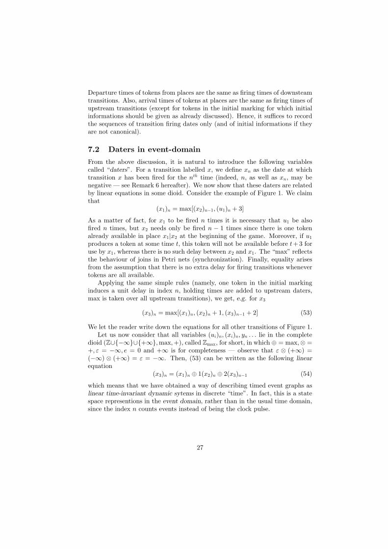
From the above discussion, it is natural to introduce the following variablescalled “daters”. For a transition labelled x, we define xn as the date at whichtransition x has been fired for the nth time (indeed, n, as well as xn, may benegative — see Remark 6 hereafter). We now show that these daters are relatedby linear equations in some dioid. Consider the example of Figure 1. We claimthat

(x1)n = max[(x2)n−1, (u1)n + 3]

As a matter of fact, for x1 to be fired n times it is necessary that u1 be alsofired n times, but x2 needs only be fired n − 1 times since there is one tokenalready available in place x1|x2 at the beginning of the game. Moreover, if u1produces a token at some time t, this token will not be available before t+ 3 foruse by x1, whereas there is no such delay between x2 and x1. The “max” reflectsthe behaviour of joins in Petri nets (synchronization). Finally, equality arisesfrom the assumption that there is no extra delay for firing transitions whenevertokens are all available.

Applying the same simple rules (namely, one token in the initial markinginduces a unit delay in index n, holding times are added to upstream daters,max is taken over all upstream transitions), we get, e.g. for x3

(x3)n = max[(x1)n, (x2)n + 1, (x3)n−1 + 2] (53)

We let the reader write down the equations for all other transitions of Figure 1.Let us now consider that all variables (ui)n, (xi)n, yn . . . lie in the complete

dioid (Z∪{−∞}∪{+∞},max,+), called Zmax, for short, in which ⊕ = max,⊗ =+, ε = −∞, e = 0 and +∞ is for completeness — observe that ε ⊗ (+∞) =(−∞) ⊗ (+∞) = ε = −∞. Then, (53) can be written as the following linearequation

(x3)n = (x1)n ⊕ 1(x2)n ⊕ 2(x3)n−1 (54)

which means that we have obtained a way of describing timed event graphs aslinear time-invariant dynamic sytems in discrete “time”. In fact, this is a statespace representions in the event domain, rather than in the usual time domain,since the index n counts events instead of being the clock pulse.

27

7.3 Counters in time-domain

Actually all trajectories produced by such systems are monotone (nondecreas-ing) functions of n since we decided to number events in the order as they occur.Monotone functions are “essentially” invertible (there is a problem with hori-zontal pieces of the graph which requires some care) and we may consider theinverse functions. These are functions of time, denoted by t (hence the timedomain), and values are interpreted as numbers of events (hence the name of“counters” for the corresponding variables).

Remark 6 Actually, counters may be initialized at null or even negative values,and they are incremented by one at each occurrence. Therefore, when we speakof a “number n” of events, we do not mean that n events occurred, but ratherthat the value of the corresponding counter is n. To avoid this confusion, weprefer to speak of an ”event of number n” and n may be negative. In the sameway, the origin of time, and hence t, may be negative. ¤We refer the interested reader to Caspi and Halbwachs [1] who introduced thisduality of points of view between time and event domains very formally, and towhom we borrowed the terminology of daters and counters. Here we providea direct introduction to counters and to the corresponding equations withoutreference to the previous section. A careful connection between counter anddater equations should be established, but it will not be discussed here sincewe are going to abandon both points of view and to introduce a new two-dimensional domain later on.

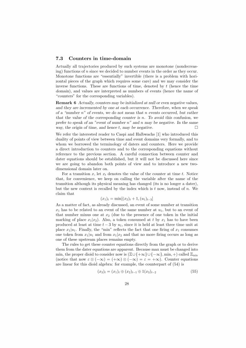
For a transition x, let xt denotes the value of the counter at time t. Noticethat, for convenience, we keep on calling the variable after the name of thetransition although its physical meaning has changed (its is no longer a dater),but the new context is recalled by the index which is t now, instead of n. Weclaim that

(x1)t = min[(x2)t + 1, (u1)t−3]

As a matter of fact, as already discussed, an event of some number at transitionx1 has to be related to an event of the same number at u1, but to an event ofthat number minus one at x2 (due to the presence of one token in the initialmarking of place x1|x2). Also, a token consumed at t by x1 has to have beenproduced at least at time t− 3 by u1, since it is held at least three time unit atplace x1|u1. Finally, the “min” reflects the fact that one firing of x1 consumesone token from x1|u1 and from x1|x2 and that no more firing occurs as long asone of these upstream places remains empty.

The rules to get these counter equations directly from the graph or to derivethem from the dater equations are apparent. Because max must be changed intomin, the proper dioid to consider now is (Z∪{+∞}∪{−∞},min,+) called Zmin(notice that now ε ⊗ (−∞) = (+∞) ⊗ (−∞) = ε = +∞). Counter equationsare linear for this dioid algebra: for example, the counterpart of (54) is

(x3)t = (x1)t ⊕ (x2)t−1 ⊕ 1(x3)t−2 (55)

28

but it should be kept in mind that the meaning of variables and of the sign ⊕has changed.

Remark 7 The passage from max to min is a nonlinear transformation asshown by the formula min(x, y) = −max(−x,−y) which can be translated withZmax notations into min(x, y) = (x−1 ⊕ y−1)−1. The passage from daters tocounters (inverse functions) is also a nonlinear transformation. But, there is analgebra suited to each domain so that equations remain linear. ¤

8 A 2-D domain and the MinMax¿γ, δÀ algebra

8.1 Informations about events

We have seen that the type of events one need to consider in a timed eventgraph may be reduced to transition firings. We thus label a type of event by thename of the corresponding transition. For a transition x, we consider “piecesof informations” about events as pairs of integers (n, t)x. What should be theinterpretation of such a piece of information? As we have already seen, thegraph carries pieces of information from upstream to downstream transitions.At a given transition, we “add” informations in the sense of simply taking theunion of informations available a priori or coming from upstream.

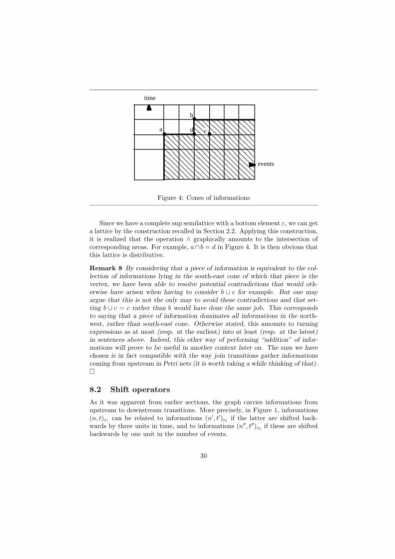
But then we face the following problem. It may happen that, at a join, theinformation coming from left is, say, b = (3, 3) whereas that coming from rightis c = (4, 2) (see Figure 4). If we interpret the pair (n, t) as “event of number noccurred exactly at time t”, there will be a contradiction since b and c are noton the graph of a nondecreasing function. But the contradiction is resolved if werather interpret (n, t) as “at time t, the number of the last event that occurredis at most n”, or equivalently “the event of number n occurred at the earliestat time t”. If we do so, then the piece of information b strictly dominates c inthe sense that b ⇒ c (think about it!), that is b ∪ c = b. In fact b dominatesall informations represented by points in the south-east cone of which b is thevertex in the 2-D domain of Figure 4. However, in the same figure, a and b doesnot dominate each other and a ∪ b (represented by the shaded area) is strictlystronger than b or a alone.

Clearly, we are introducing an idempotent addition (the union) over piecesof information, to which a partial order can be associated as in Theorem 1. Forthis addition to be an inner operation, we have to define the set of informationsas the set of finite union of pieces of informations (union of cones), and for thissemilattice to be complete, we have to extend the definition to infinite unions.The order is simply inclusion. There is a null element which is the informationdominated by any other one, namely ε = (+∞,−∞), which may be phrased“the event of number ∞ occurred at the earliest at the beginning of times”,which indeed says nothing about the behaviour of the sytem.

29

a

b

c

time

events

d

Figure 4: Cones of informations

Since we have a complete sup semilattice with a bottom element ε, we can geta lattice by the construction recalled in Section 2.2. Applying this construction,it is realized that the operation ∧ graphically amounts to the intersection ofcorresponding areas. For example, a∩ b = d in Figure 4. It is then obvious thatthis lattice is distributive.

Remark 8 By considering that a piece of information is equivalent to the col-lection of informations lying in the south-east cone of which that piece is thevertex, we have been able to resolve potential contradictions that would oth-erwise have arisen when having to consider b ∪ c for example. But one mayargue that this is not the only may to avoid these contradictions and that set-ting b ∪ c = c rather than b would have done the same job. This correspondsto saying that a piece of information dominates all informations in the north-west, rather than south-east cone. Otherwise stated, this amounts to turningexpressions as at most (resp. at the earliest) into at least (resp. at the latest)in sentences above. Indeed, this other way of performing “addition” of infor-mations will prove to be useful in another context later on. The sum we havechosen is in fact compatible with the way join transitions gather informationscoming from upstream in Petri nets (it is worth taking a while thinking of that).¤

8.2 Shift operators

As it was apparent from earlier sections, the graph carries informations fromupstream to downstream transitions. More precisely, in Figure 1, informations(n, t)x1 can be related to informations (n′, t′)u1 if the latter are shifted back-wards by three units in time, and to informations (n′′, t′′)x2 if these are shiftedbackwards by one unit in the number of events.

30

Therefore, we associate a backward (elementary) operator (m, d)y|x to everyarc or place y|x, where m takes the value of the number of tokens in the initialmarking and d takes the value of the holding time. Then a piece of information(n, t)x yields a piece of information (n′, t′)y = (m, d)y|x.(n, t)x := (n+m, t+ d).The definition is extended in a straightforward manner to “sums” of pieces ofinformations by distributivity. It is also immediate to define the “sum” of twoshift operators fy|x and gy|x in a usual way by summing up the informationsproduced by the two operators from the same information ix. This correspondsto two parallel arcs between x and y in the graph. General (nonelementary) shiftoperators are defined as (finite or infinite) sums of elementary operators. Twoarcs in series y|x and z|y provide a way of defining the “product” of operatorsas the usual composition of applications. Obviously, (m′, d′)z|y◦(m, d)y|x = (m+m′, d+ d′). There is an identity operator represented by (0,0). The product ofoperators distributes over sum.

It is not hard to realize that we are just about constructing a dioid structurefor shift operators. But it is possible to extend this structure to informations(observe that we already defined the sum of informations which behaves arith-metically as the sum of operators). In fact informations and operators neednot be distinguished. As a matter of fact, we may conceptually consider thatevery information, say (n, t)x, is produced from a canonical information (0, 0)attached to a “source” transition s from which we draw an arc x|s with weight(n, t) (if n and t are counted from negative origins, these origins are put at thesource instead of (0, 0)). However this discussion is better pursued with moreconvenient algebraic notations and in a more abstract setting.

8.3 Coding informations and shift operators

A collection of informations {(ni, ti) | i ∈ I ⊂ N} about a type of event isa collection of points in the plane depicted on Figure 4. It may be seen asa pointwise measure in the plane (a measure in Z2). We may represent this“discrete event measure” by its characteristic function

∑i∈I γ

niδti where thesum is a formal sum and γ and δ are formal variables. In fact, γ may beinterpreted as the backward shift operator on counting and δ as the backwardshift operator on dating. For example, by considering arcs such as x1|x2 (resp.x2|x1) in Figure 1, it can be shown that downstream discrete event measures canbe derived from upstream ones by formal multiplication of the correspondingformal power series by γ (resp. δ).

Formal addition of power series corresponds to our previous sum or unionof informations about a type of event. But we must reflect the fact that a ∪ d(resp. b∪ d) in Figure 4 is equal to a (resp. b). This imposes, in addition to theusual rules of formal sum and product of power series, the unusual additionalrules

γnδt ⊕ γn′δt = γmin(n,n′)δt (56)

31

γnδt ⊕ γnδt′ = γnδmax(t,t′) (57)

Notice that this is enough to get that b ∪ c = b in Figure 4 since b ∪ c =(b ∪ d) ∪ (d ∪ c) = b ∪ d = b.

We are now ready to introduce a new dioid more formally in order to providea theoretical basis to all these calculations.

8.4 The dioid MinMax¿γ, δÀWe first introduce the set of formal power series B¿γ, δÀ in two variables (γ, δ)with boolean coefficients and exponents in Z. This set will be designated by Lin the sequel. Observe that this is a dioid. In particular the sum is idempotentsince coefficients are boolean, ε corresponds to the series with coefficients allequal to zero and e = γ0δ0. Graphically, an element of L is represented by acollection of points in Z2: a monomial γnδt with boolean coeffficient 1 yieldsa point with coordinates (n, t); null boolean coefficients yield no point (henceε corresponds to the empty set and e to the origin of the plane). Additioncorresponds to union and multiplication of two elements to the vector sum ofthe associated collections of points. Order is inclusion. ∧ is intersection.

As previously observed, this dioid is not adequate for our purpose since (56)–(57) are not part of the usual calculation rules with formal power series. In fact,we wish that a point a = (n, t) in the 2-D domain, coded by the monomialγnδt, be “equal” to the whole south-east cone of vertex a. But this cone iscoded by γnδtγ∗(δ−1)∗ (recall the definition (32) of the star). Observe thatγ∗(δ−1)∗ = (γ⊕δ−1)∗ from (49). We are thus led to consider the dioid L moduloγ ⊕ δ−1 based on Definition 9 and Theorem 20.

Definition 10 The dioid MinMax¿γ, δÀ, designated hereafter by M forshort, is the dioid L/(γ ⊕ δ−1).

Comments

(i) This dioid is commutative, complete and distributive. All these propertiescan be checked easily. The graphical interpretations of ⊕, ∧ and ⊗ as ∪,∩ and vector sum respectively are still valid, but they now apply to unionsof south-east cones.

(ii) Starting from the formal definition of M, it is easy to check that all cal-culations can be performed practically using the usual the rules of formalpower series and the additional rules (56)–(57). It should be kept in mindthat an element of M is an equivalence class. Therefore it has severalformal representations. For example, e = γ∗(δ−1)∗ = γ∗ = (δ−1)∗ =γ∗ ⊕ (δ−1)∗ = γ0 = δ0 = γ0δ0 in M but not in L! Indeed, in each equiva-lence class, there is a minimal and a maximal representatives, “minimal”and “maximal” referring to the order in L. The minimal representativeis obtained by coding only the extremal north-west points of the shaded

32

area in Figure 4. The maximal one is obtained by coding all the pointsin the shaded area. This maximal representative is obtained algebraicallyby multiplication of any representative by γ∗(δ−1)∗ (see last statement ofTheorem 20).

(iii) Let us consider how to calculate a ∧ b in M. First of all, since the dioidis distributive, it suffices to know how to calculate that expression whena and b are monomials. Then it can be checked that

γnδt ∧ γn′δt′ = γmax(n,n′)δmin(t,t′) (58)

which should be compared with (56)–(57). Notice that ⊗ does not dis-tribute over ∧ in general, although this is true for multiplication by mono-mials.

(iv) In a general complete dioid, let us introduce the following notation (com-pare with (32))

a∧ := e ∧ a ∧ a2 ∧ . . . (59)

Then, coming back to M, consider the following table

γ+∞ ∼ γ∧

γ−∞ ∼ (γ−1)∗

δ+∞ ∼ δ∗

δ−∞ ∼ (δ−1)∧

γ+∞δ−∞ ∼ ε

γ−∞δ+∞ ∼ ∞

It is not difficult to realize that elements in the left-hand side formallybehave as their corresponding elements in the right-hand side, the latterbeing well-defined in M. Therefore, we may take the right-hand expres-sions as definitions for the left-hand notations. The only additional rulesto keep in mind are the following

γ−∞γ+∞ = γ+∞ (60)δ−∞δ+∞ = δ−∞ (61)

These rules can easily be proved from the definitions.

(v) M is not Archimedian. A counterexample is the following

γnδ−∞ ⊗∞ = γ−∞δ−∞ 6=∞

which contradicts Theorem 2. ¤

33

9 Input-output representation in the 2-D do-main

9.1 System equations and transfer matrices

Consider an event graph as in Figure 1. To each transition, we associate anelement of M which codes the whole set of informations available about the(generally infinite) sequence of events related to this transition. This elementwill be called after the name of the transition (e.g. x1) but it should be keptin mind that it is different from a dater or a counter, and that it is a powerseries in two variables with positive (and possibly negative) exponents (indeedan equivalence class). If necessary, to recall this, we may sometimes say x1(γ, δ)instead of x1.

From all that have been said until now, it should be clear that the followingequations can be obtained for the case of Figure 1 x1

x2x3

=

ε γ εδ ε εe δ γδ2

x1x2x3

⊕ δ3 ε

ε γδε ε

( u1u2

)

y =(ε γ δ3

) x1x2x3

(62)

In general, for any event graph, we get the following equations

x = Ax⊕Bu y = Cx (63)

where x, y (resp. A,B,C) are column vectors (resp. matrices) of appropriatedimensions with entries in M.

The former equation is an implicit equation of the form (31). We know thatit has no unique solution in general. However, we are interested in the smallestsolution since this corresponds to the earliest possible dates for events (recallthat we assumed that transitions are fired as soon as they can). Using Theorem9-(i), we conclude that x = A∗Bu and

y = CA∗Bu (64)

This completely specifies the input-output behaviour of the system: for giveninformations about the input transitions (they must be activated from outside),informations about the earliest possible outputs are calculated. The matrixH := CA∗B is called the “transfer matrix” of the system. Its expression hasbeen given in (1) for the case of Figure 1.

In general, Hij corresponds to the “trajectory” of yi for all inputs uk = εexcept for uj = e. In conventional system theory, it is called the “impulse

34

(a) (b) (c)

canonicalinitial

informations

non canonicalinitial

informations

controllinginitial tokens

y

u u

y y

u

v

w

response” from j to i. Here, an input ε = γ+∞δ−∞ can be interpreted as aninfinity of tokens available in an imaginary place upstream the correspondinginput transition since the beginning of times. This is the least constraininginput one can imagine. On the other hand, an input e = γ∗ may be called animpulse at time 0. Before time 0, the input transition is frozen, and then aninfinity of tokens are made available. Notice that tokens (or transition firings)are numbered from 0, not from 1, since e = γ0δ0 ⊕ γ1δ0 ⊕ · · ·

9.2 About initial informations

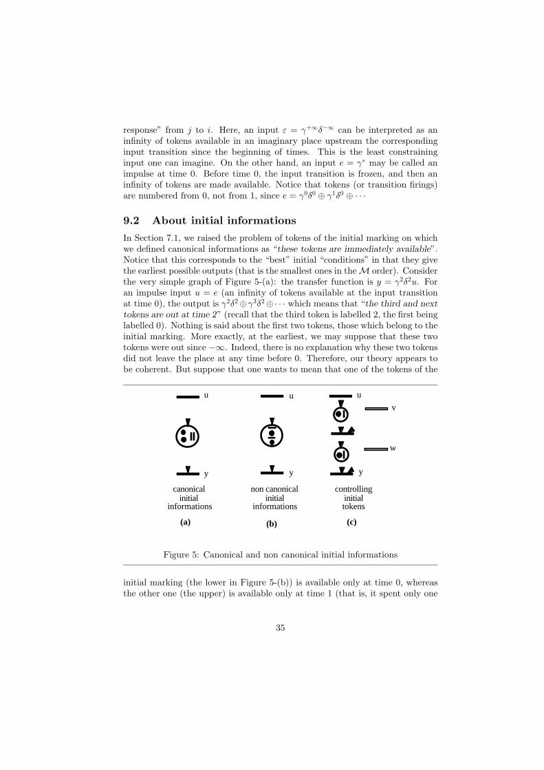
In Section 7.1, we raised the problem of tokens of the initial marking on whichwe defined canonical informations as “these tokens are immediately available”.Notice that this corresponds to the “best” initial “conditions” in that they givethe earliest possible outputs (that is the smallest ones in theM order). Considerthe very simple graph of Figure 5-(a): the transfer function is y = γ2δ2u. Foran impulse input u = e (an infinity of tokens available at the input transitionat time 0), the output is γ2δ2⊕γ3δ2⊕· · · which means that “the third and nexttokens are out at time 2” (recall that the third token is labelled 2, the first beinglabelled 0). Nothing is said about the first two tokens, those which belong to theinitial marking. More exactly, at the earliest, we may suppose that these twotokens were out since −∞. Indeed, there is no explanation why these two tokensdid not leave the place at any time before 0. Therefore, our theory appears tobe coherent. But suppose that one wants to mean that one of the tokens of the

Figure 5: Canonical and non canonical initial informations

initial marking (the lower in Figure 5-(b)) is available only at time 0, whereasthe other one (the upper) is available only at time 1 (that is, it spent only one

35

time unit in the place at the beginning of the game). This may be representedas shown in (b). To come back to canonical initial informations, we can drawthe expanded graph of Figure 5-(c) where it is necessary to add the grey inputtransitions v and w. Without these controls, the two tokens would again be ableto leave the sytem at any time before 0 (the transfer function would again beγ2δ2). Now it is y = w⊕γδ(v⊕γδu). To release the tokens only at time 0, we setv = w = e and we get y = e⊕ γδ ⊕ γ2δ2u. The input-output relationship is thesame as in the previous case but we have the additional informations that thefirst token leaves at time 0 and the second at time 1 (this is more informationsthan previously and indeed this new y is larger than the previous one in theM order). We invite the reader to consider the same kind of non canonicalinitial informations but for tokens in a loop. Notice that we permanently usedthe expression “initial informations” rather than “initial conditions” becausevariables are attached to transitions whereas these informations are attached totokens of the initial marking.

9.3 Circulation of tokens

Consider e.g. the event graph of Figure 1. Suppose that we bring only one tokenat the input transition u1 at time 0. The corresponding inputs are u1 = e⊕γδ+∞

and u2 = δ+∞ and the output calculated with (1) is y = δ8 ⊕ γδ+∞, indicatingthat a single token has been released at time 8. Then the system is stabilized,but with a new marking: since all transitions, but u2, have been activated once,all places have the same marking as initially except for x2|u2 where the tokenhas disappeared. If we calculate the new transfer matrix for this new “initialmarking”, we find that H1 is unchanged, but that H2 is divided by γ withrespect to the previous one appearing in (1). The explanation is that changingthe origins of daters and of counters has no effect on the transfer matrix providedthat the same change be applied to all input and output transitions. This iswhat occurred in our example for the pair (u1, y) since both have been firedonce. But the rule is not fulfilled for (u2, y), hence the change in H2.

Consider again the experiment of bringing one token at u1 at time 0 fromthe initial situation of Figure 1. At time 2, the token is still in place x1|u1since it must stay 3 time units there, and no other transition has been fired sofar. From what has been said above, it can be predicted that if we write downthe equations for this new situation, considering canonical initial informations(which anyway do not affect the transfer matrix), we shall find the same H2, buta H1 which is multiplied by γ. Let us consider this new transfer matrix, say H,as the reference for what follows. Just after time 3, transition x1 will have beenfired, taking off one token from places x1|u1 and x1|x2 and adding one tokenin places x3|x1 and x2|x1. This new transition firing which has affected onlyan inner transition should not modify H. This can be checked by the reader.Of course, this will not be the case if transitions are fired by adding tokensin upstream places directly from outside, that is without passing through input

36

transitions. This may cause a dramatic change of the transfer matrix, especiallyif it affects the number of tokens in each circuit which is invariant for any eventgraph.

The fact that regular firings of inner transitions which move tokens arounddo not affect the transfer matrix is reminiscent of the well-known fact of con-ventional system theory that a linear change of basis in the state space does notmodify the input-output relationship. Although we have not considered transfermatrices (in a single variable) corresponding to either dater or counter “statespace” equations yet (this will come later on), we invite the reader to checkwhether those transfer matrices are not affected by inner circulations of tokens,and possibly to find out the corresponding state space basis change. It turnsout that the answer is yes only with the counter approach. Notice that tokensof the initial marking cause delays in dater equations whereas they appear ascoefficients in counter equations. Coming back to our 2-D domain, we let thereader check that, if transition xi is regularly fired once, the new matrices, sayA, B, C, obtained by writing down equations after this firing are related to theprevious A,B,C by the relations

A = M−1AM B = M−1B C = CM

where M is a diagonal matrix with Mjj = e for j 6= i and Mii = γ. As a matterof fact, firing xi produces one token more (multiplication by γ) — resp. onetoken less (multiplication by γ−1) — in all downstream — resp. upstream —transitions (indicated by the nonnull entries of column A.i — resp. of row Ai.).The new matrices contain no entries with negative exponents iff the transitionfiring is regular.

10 Output targets and the adjoint system

10.1 The problem of output targets as a residuationproblem in M

Instead of specifying input informations and calculating the earliest (smallest)resulting output, we may rather impose output targets and search for the latest(greatest) input that meets these specifications. More precisely, for a specifiedtarget z (a column vector the dimensionality of which is the number of outputtransitions, say p), we pose the following problem

Find the greatest v such that CA∗Bv ≤ z (65)

where v has the dimensionality of the number of input transitions. This isreminiscent of Definition 7 of residuation and one has that v = (CA∗B)\z.

There is however a point which deserves some attention. An elementarytarget specified by a pair (n, t) should be interpreted as “the event of number n

37

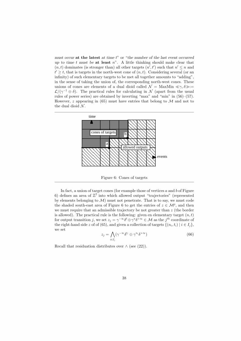
a

b

time

events

allowed outputs

cones of targets

must occur at the latest at time t” or “the number of the last event occurredup to time t must be at least n”. A little thinking should make clear that(n, t) dominates (is stronger than) all other targets (n′, t′) such that n′ ≤ n andt′ ≥ t, that is targets in the north-west cone of (n, t). Considering several (or aninfinity) of such elementary targets to be met all together amounts to “adding”,in the sense of taking the union of, the corresponding north-west cones. Theseunions of cones are elements of a dual dioid called N = MaxMin ¿γ, δÀ:=L/(γ−1 ⊕ δ). The practical rules for calculating in N (apart from the usualrules of power series) are obtained by inverting “max” and “min” in (56)–(57).However, z appearing in (65) must have entries that belong to M and not tothe dual dioid N .

Figure 6: Cones of targets

In fact, a union of target cones (for example those of vertices a and b of Figure6) defines an area of Z2 into which allowed output “trajectories” (representedby elements belonging toM) must not penetrate. That is to say, we must codethe shaded south-east area of Figure 6 to get the entries of z ∈ Mp, and thenwe must require that an admissible trajectory be not greater than z (the borderis allowed). The practical rule is the following: given en elementary target (n, t)for output transition j, we set zj = γ−∞δt⊕γnδ+∞ ∈M as the jth coordinate ofthe right-hand side z of of (65), and given a collection of targets {(ni, ti) | i ∈ Ij},we set

zj =∧i∈Ij

(γ−∞δti ⊕ γniδ+∞) (66)

Recall that residuation distributes over ∧ (see (22)).

38

10.2 Solving the target problem with the adjoint system

Notice that since the rules for “adding” a collection of elementary targets{(ni, ti) | i ∈ Ij} (represented by an element of N ) are dual of those for addinga collection of pieces of informations, it would suffice to code this collection oftargets as

ηj =⊕i∈Ij

γ−niδ−ti (67)

to come back into M. The minus signs in the exponents have the desiredeffect of inverting “max” and “min” in calculations and this correspondence isobviously an isomorphism between dioids N and M. Then the question arisesof the relationship of z given by (66) with η given by (67) which are two differentways of coding targets in M.

Lemma 5 Let ϕ := γ−∞δ0 ⊕ γ0δ+∞ ∈ M. Then the p-dimensional columnvector with entries zj given by (66) is related to the row vector with entries ηjgiven by (67) by zj = ηj = ηj\ϕ.

The proof is straightforward using formula (21) and the fact that residuationby monomials (say γ−nδ−t) amounts to multiplication by the inverse γnδt. Thisis an example where residuation is easy to perform.

As a consequence of this lemma and the discussion around formula (29) inSection 3.3, the solution v of problem (65) can be obtained as follows (we use“tilde” on vectors with an obvious meaning — recall that column vectors yieldrow vectors by this transformation and conversely)

v = (CA∗B)\z = (CA∗B)\η = µ (68)

withµ = ηCA∗B =⇒ µ = ξB ξ = ξA⊕ ηC (69)

which is the adjoint system of (64)–(63).

Remark 9 Notice that, in (69), the implicit system in the right-hand side mustbe solved for the smallest solution if we want to replace =⇒ by ⇐⇒. This iscoherent with the fact that “smallest” in the coding (67) of targets is equivalentto “greatest” (latest) in the coding (66), that is after the transformation “tilde”.¤

10.3 Direct derivation of the adjoint system

Let us show how we could have obtained the solution of problem (65) throughformulas (68)–(69) by reasoning directly on the graph as we did to obtain equa-tions for the direct system. Consider the example of Figure 1 and the outputtransition y for which a collection of targets {(ni, ti) | i ∈ Iy} are given. It isclear that these targets can be transferred back to the upstream transitions x3

39

and x2 by subtracting 3 units from ti, respectively 1 unit from ni. That is arcswith weights (shift operators) (m, d) operate back with (−m,−d). Notice thatjoins in the direct graph are forks in the reverse graph. In the same way, forksbecome joins as for example at transition x2. Targets carried back from thedownstream transitions y, x3, x1 must be “added” using rules which are com-pletely dual of those for adding informations as already discussed. Finally, wesee that we must operate with a dual algebra and with shift operators whichhave negative signs. Instead of that, we may decide that we are going to changethe signs of all equations so that we come back to the previous algebra, shift op-erators get back their positive signs, but a collection of targets is now recordedas {(−ni,−ti)}. This corresponds exactly to the coding (67) and to equations(69), where the original algebraM and the original operators A,B,C (not their“opposite”) are used, but where vectors are row vectors operating on the leftof operators (because we must anyway scan the graph from output to inputtransitions).

11 Rationality, realizability and periodicity

11.1 A fundamental theorem

A timed event graph as that of Figure 1 can be represented as a finite-dimensional linear invariant system (63) which in turn can be represented by atransfer matrix (64).

Remark 10 If there are direct arcs from input transitions to output transitions,we get an output equation of the form y = Cx ⊕ Du and a transfer matrixCA∗B ⊕ D. However, by redefining the “state” vector as x = (xT , uT )T , itis possible to come back to the form CA∗B but at the price of increasing the“state” dimensionality. This has no importance in what follows since we are notgoing to deal with the problem of “minimal” realizations. ¤

Observe that for a realistic (“causal”) event graph, entries of A,B,C are poly-nomials ofM involving only nonnegative exponents. These polynomials belongto the “dioid closure” of the “generating subset” E = {ε, e, γ, δ}. This motivatesthe following definition of rationality.

Definition 11 (Rationality) A matrix or a vector with entries in M is saidrational iff its entries lie in the subdioid E∗ ⊂ M (rational closure of E :={ε, e, γ, δ} — see Definition 8).

Definition 12 (Realizability) A p × m-dimensional matrix H in M is saidrealizable iff it can be written

H = C(γA1 ⊕ δA2)∗B (70)

40

where C and B are matrices of respective dimensions p× n and n×m, n beingan arbitrary but finite integer, A1, A2 are n× n, and the entries of all matriceslie in {ε, e}.

Definition 13 (Periodicity) An element h ofM is said periodic iff there existnonegative and finite integers ν, τ, r, s (r and s not both null) such that h canbe written as

h = Pν−1,τ−1 ⊕ [γνδτ ⊗Qr−1,s−1 ⊗ (γrδs)∗] (71)

where Qr−1,s−1 stands for a polynomial in (γ, δ) with nonnegative exponents ofdegrees not greater than (r − 1, s − 1), and Pν−1,τ−1 has a similar meaning. Amatrix H is periodic iff all its entries are periodic.

The intuitive meaning of formula (71) considered as an impulse response is thefollowing. There is a transient behaviour represented by P , followed by a peri-odic behaviour in which a pattern represented by Q is indefinitely reproducedaround an asymptotic slope s/r. This ratio represents the asymptotic outputrate of the response: in the average, r tokens get out each s time units.

If s = 0, the impulse response is polynomial since (γp)∗ = e : this is thebehaviour of a purely “moving average” system (no circuit in the graph). Noticethat, here, thinking of a “polynomial impulse response” as a “finite impulseresponse”, as it is familiar in conventional system theory, may be misleading:for an “impulse” at the input, that is an infinity of tokens brought at time 0,there is a transient (some tokens get out as indicated by the polynomial), andthen an infinity of tokens get out all together.

If r = 0, since (δs)∗ = δ+∞, the response is “frozen” after a possible transientduring which some tokens get out (this may rather be the kind of behaviour onewould like to call a “finite response”). This happens when there is a circuitwithout token which is blocking the output transition.

Theorem 21 For H ∈Mp×m, the following three statements are equivalent

(i) H is realizable

(ii) H is rational

(iii) H is periodic

Proof The implication (i) ⇒ (ii) is straightforward. The converse (ii) ⇒ (i)follows, at least for the single-input single-output (SISO) case, from Theorem14 with B = C = {ε, e}. It remains to split up matrix Ax which appears inthe (B, C)-representation (45) into γA1 ⊕ δA2 which offers no difficulty. For themultiple-input multiple-output (MIMO) case , it suffices to realize the SISOtransfer for each input-output pair individually, and then to concatenate theserealizations, since we do not worry about minimality.

It remains to prove the equivalence (ii) ⇔ (iii). Since the definitions ofperiodicity and rationality refer to the entries of H individually, it suffices to

41

deal with the SISO case. The implication (iii) ⇒ (ii) is obvious: if h can bewritten as (71), then clearly h ∈ E∗. Conversely, if h is rational, since M is acommutative dioid, we can use Theorem 19 (applied to the dioid closure of E)to see that h can be written as

h =⊕i∈I

γαiδβi(⊕j∈Ji

γrj δsj )∗

=⊕i∈I

γαiδβi⊗j∈Ji

(γrj δsj )∗ (72)

where I and the Ji’s are finite sets, αi, βi, rj, sj are nonnegative integers and(72) follows from (49). The proof will be complete if we show that (72) can bereduced to (71): roughly speaking, this amounts to saying that some (γrj δsj )∗,essentially the one for which the “slope” sj/rj is the greatest, asymptotically“absorbs” all other terms of the same type to which it is added or which itmultiplies. This is what is explained in the next technical lemma. ¤

Lemma 6 InM, expressions of the form (72) can always be reduced to expres-sions of the form (71).

Outline of proof This lemma can be proved in three steps. First, for givenpositive integers r, r′, s, s′

[s/r > s′/r′] =⇒ [∀α, α′, β, β′,∃N : ∀n′ ≥ N, ∃n : γαδβ(γrδs)n ≥ γα′δβ′(γr′δs′)n′ in M]

From this result,it is then proved that expressions of the form γαδβ(γrδs)∗ ⊕ γα

′δβ′(γr

′δs′)∗ or

(γrδs)∗(γr′δs′)∗ can be reduced to expressions of the form P (γ, δ)⊕Q(γ, δ)(γrδs)∗,

where P (γ, δ) and Q(γ, δ) are polynomials in (γ, δ). Essentially the same thingcan be proved when s/r = s′/r′ except that now the reduced expression isP ⊕ Q(γr

′′δs′′)∗ where r′′ (resp. s′′) is the least common multiple of r and r′

(resp. s and s′). Finally, it remains to check that those expressions can bereduced to expressions like (71) for which additional conditions on the degreesof P and Q and on the valuation of Q must be met. ¤

Comments

(i) In the proof of Theorem 21, instead of proving the implication (ii) ⇒(iii), we might have proved the implication (i) ⇒ (iii) using Theorem 18and formula (51). This gives additional insight into how the unique term(γrij δsij )∗ appearing in the representation (71) of each Hij is related to theweights of circuits of matrix A = γA1 ⊕ δA2 appearing in (70). For aninput-output pair (uj, yi), we consider all (oriented) paths connecting thesetransitions and all circuits which have at least one node (i.e. transition) incommon with those paths. These are the circuits of interest to determinethe maximal ratio sij/rij . If there is no such circuit, this means that the

42

polynomial Q of (71) is null and (γrij δsij )∗ is irrelevant. As a consequence,if matrix A is strongly connected (which in particular precludes any directpath from the input to the output, given that we have not included a termDu — see Remark 10), then there is a unique (γrδs)∗ for the whole transfermatrix H.

(ii) In the definition of realizability, we might have required the weaker condi-tion that H = CA∗B with entries of A,B,C be simply polynomials withnonnegative exponents (this would be called a polynomial representation).The “inner” dimension would then be smaller than above in general for agiven H. This corresponds to choosing E as the dioid closure of {ε, e, γ, δ}and to taking B and C identical to E . In fact, there is a lot of otherintermediate possibilities (see the comments at the end of Section 4.2).¤

11.2 The eigenvalue problem in the 2-D domain

We have seen that the impulse response of a finite-dimensional linear invariantsystem typically consists of a transient followed by a periodic behaviour whichis characteristic of the system. Usually, for an autonomous linear system, char-acteristic behaviours are associated with eigenvalues, and transients are avoidedby starting with initial conditions corresponding to eigenvectors.

Consider the autonomous system xn+1 = Axn in the event domain (recallthat the algebra is Zmax). The eigenvalue problem Ax = λx has been extensivelystudied in [2, 3]. Essentially, for a matrix A representing a strongly connectedgraph, there exists a unique eigenvalue λ which is equal to the maximal ratios/r over all circuits of the graph (s is again the number of time units and r isthe number of tokens of the initial marking along a circuit). For non stronglyconnected graphs, say for a graph with two strongly connected components, it iseasy to figure out that there are two eigenvalues if the critical circuit belongs tothe upstream component (the two eigenvalues are those of the two componentsconsidered separately) whereas there is only one eigenvalue (the largest one) ifthe critical circuit is downstream. The structure of the “eigenspace” has alsobeen extensively studied.

An eigenvalue λ = s/r means that, in the average, each component of xn(the dater) is incremented by s time units every time n (the counter) is increasedby r. In the 2-D domain, we have to say something similar. Recall that nowx represents the whole trajectory. If a trajectory extending from −∞ to +∞can “slide” along itself by translations (r, s) or (−r,−s) without changing, it isinvariant when multiplied by any positive or negative power of the monomialγrδs. An elegant way to say this is to appeal once again to the “calculus modulo”introduced in Section 6. More precisely, we have to check that [x]γrδs⊕γ−rδ−s ispolynomial, each polynomial entry representing a pattern which is repeatedindefinitely. This justifies the following definition.

Definition 14 We say that a pair of positive integers (r, s) is an eigenvalue of

43

the square matrix A with rational — see Definition 11 — and polynomial entriesiff there exists a vector x with the same kind of entries, which is not identicallynull and such that

x = Ax in M/(γrδs ⊕ γ−rδ−s) (73)

When calculating inM/(γrδs⊕ γ−rδ−s), in addition to the rules (56)–(57), oneis allowed to replace every positive or negative power of γrδs by e since they allfall in the same equivalence class (thanks to (36)–(37)). Also, because of thecommutative diagram of Figure 2, all these simplification rules can be used inany order.

Theorem 22 Let A be a square matrix with rational and polynomial entriesand assume that A is represented by a strongly connected graph. Then, thereexists an eigenvalue (r, s), and for this eigenvalue the ratio s/r is maximal overall circuits of the graph (in this sense, the eigenvalue is unique).

Outline of proof This statement is a direct consequence of formula (40). Thisformula gives the general form of an x verifying (39). To prove existence ofan eigenvector, we set yκ = 0 for all circuits except that or those achievingthe maximal ratio s/r for which we set, say, yκ = e. We then use Lemma 6and we calculate modulo γrδs ⊕ γ−rδ−s if the critical circuit is unique and hasweight (r, s), or we appeal to the least common multiples of all critical pairs(r, s) otherwise (see the explanations following Lemma 6). The resulting x ispolynomial and rational and it verifies (73).

Conversely, suppose that x verifies (73) for some pair (r, s). This meansthat ~x := (γrδs)#x verifies (39) and thus, from Theorem 12, it can be identifiedwith an expression of the form (40). A contradiction arises when passing tothe equality of those two expressions of ~x modulo γrδs ⊕ γ−rδ−s if one assumesthat s/r is not the maximal ratio over all circuits. This contradiction is basedon the observation that (γr

′δs′)∗ (mod γrδs ⊕ γ−rδ−s) cannot be polynomial if

s′/r′ > s/r. ¤

11.3 Transfer matrices associated to dater and counterequations

The following notations refer to those introduced in Section 4.3. Let us keepB = C = {ε, e} and let F = {ε, e, δ},G = {γ}. It is obvious that the dioid F∗is isomorphic to the (complete) dioid (N ∪ {−∞} ∪ {+∞},max,+) denoted byNmax for short. Moreover, F∗⊗B and C⊗F∗ are identical to F∗ whereas F∗⊗Greduces to the set of elements of the form aγ where a ∈ Nmax.

Remark 11 We might have started with G = {e, γ, γ2, . . .}, in which case F∗⊗G would amount to the set of polynomials in γ with coefficients in Nmax. The restof the discussion could be carried on, with some adaptations, in this situation.¤

44

An observer (resp. controller) representation (see Theorem 16) is of the formC(γA)∗B where we may consider that the entries of A and B (resp. C) are inNmax, those of C (resp. B) are in {ε, e}. This can be viewed as the transfermatrix corresponding to the following dater equations (the algebra is Nmax)

xn+1 = Axn ⊕Bun+1 yn = Cxn

and γ appears as the unit backward shift operator in the event domain.Let Zmax¿γÀ be the set of formal power series in γ with coefficients in

Zmax. Consider the correspondence γnδt 7→ tγn which associates to a monomialin (γ, δ) (with boolean coefficient 1) a monomial in Zmax¿γÀ. This is extendedin an obvious manner to formal power series. Recall the calculations rules (56)–(57) inM and notice that calculating in Zmax¿γÀ amounts to taking the latterinto account but not the former. That is to say, we must introduce the followingadditional rule in Zmax¿γÀ

aγn ⊕ aγn′ = aγmin(n,n′)

This of course can be done more formally by introducing an equivalence relation.Coming back to state space equations, it is realized that an equation like xm =axm−n ⊕ axm−n′ can be simplified into xm = axm−min(n,n′), which is easy tounderstand directly.

All these considerations can dually be made with counter equations (timedomain) by inverting the role of γ and δ when defining F and G, by changingNmax into Nmin (with an obvious definition of the latter) and Zmax¿γÀ intoZmin¿δÀ, by introducing dual calculations rules, etc. . . In our opinion, the2-D domain offers a complete symmetry between counting and dating which issomewhat lost when projecting in either one-dimensional domain.

12 Conclusion

In this paper, we have attempted to provide a unified introduction to unusual,albeit not new, algebraic tools, and to show how they can be used in the con-struction of a new “linear” system theory. This theory encompasses systemsthat can otherwise be described as event graphs, a special class of Petri nets.Essentially, in this class, logical “and” can be modelled easily, but not logical“or”, unlike in Automata theory. However, time and events can be manipulatedsimultaneously. Anyway, event graphs appear as the class of Petri nets that are“linear” when using dioid algebras. We have shown several ways of modellingthem (in the event domain, in the time domain and in a 2-D domain) and adifferent algebra has to be used in each approach, but all fall into the categoryof dioids.

We have tried to give a sufficiently self-contained presentation, and somealgebraic results appear here for the first time. However, there was no attempt

45

to be exhaustive. On the algebraic side, we did not discuss such issues as “lineardependence” in “vector spaces” on dioids (sets Dn with an internal addition ⊕and an external multiplication ⊗ by scalars in D). This issue is basic for thesystem-theoretic issue of “minimal realizations”, a question which is still open(see however [14]). There are several possible definitions of linear dependence[13] and one of them can be characterized by the condition of some “determi-nant” being null [9]. We did not either discuss the Cayley-Hamilton theorem(see [12, 16]): it holds true in dioids simply because of the proof of Straubing[18] which is based only on combinatorial properties that are common to boththe conventional and the dioid algebras. However, the formulation of Cayley-Hamilton theorem in dioids requires some care because of the lack of “minussign” in these algebras. This theorem should play an important role in realiza-tion theory.

On the system-theoretic side, apart from the basic question of minimal re-alization, we believe that control and optimization issues should be more de-velopped for this theory to prove practically useful. In this paper, we did notreview such notions as “stability” and structural controllability and observabil-ity previously introduced in the framework of dater equations, nor the associatedresults concerning stabilizability by dynamic output feedback [4]. The practicalsignificance of these results in the framework of flexible manufacturing systemswas discussed in earlier papers [2, 3].

Anyway, considering the amount of efforts that has been devoted to thedevelopment of conventional linear system theory during at least twenty years,it must be considered that this new sytem theory is just in its infancy. However,it is interesting to see how continuous systems and discrete event systems canbe essentially considered from the same points of view and concepts, providedthat the algebra be adapted. This requires a specific effort.

Acknowledgement Mr. Ramine Nikoukhah who recently joined our group(on leave from MIT) helped us in clarifying some points such as the issue ofinitial conditions. His contribution is gratefully acknowledged.

References

[1] P. Caspi and N. Halbwachs, “A functional model for describing and reason-ing about time behaviour of computing systems ”, Acta Informatica, Vol.22, pp. 595–627, 1986.

[2] G. Cohen, D. Dubois, J.P. Quadrat and M. Viot, “Analyse du comporte-ment periodique des systemes de production par la theorie des dioides”,INRIA Report No. 191, Le Chesnay, France, 1983.

[3] G. Cohen, D. Dubois, J.P. Quadrat and M. Viot, “A linear system theoreticview of discrete event processes and its use for performance evaluation in

46

manufacturing”, IEEE Trans. on Automatic Control, Vol. AC–30, pp. 210–220, 1985.

[4] G. Cohen, P. Moller, J.P. Quadrat and M. Viot, “Linear system theoryfor discrete-event systems”, 23rd IEEE Conf. on Decision and Control, LasVegas, Nevada, 1984.

[5] G. Cohen, P. Moller, J.P. Quadrat and M. Viot, “Une theorie lineairedes systemes a evenements discrets”, INRIA Report No. 362, Le Chesnay,France, 1985.

[6] G. Cohen, P. Moller, J.P. Quadrat and M. Viot, “Dating and countingevents in discrete event systems”, 25th IEEE Conf. on Decision and Control,Athens, Greece, 1986.

[7] R.A. Cuninghame-Green, “Minimax Algebra”, Springer-Verlag, Berlin,1979.

[8] P. Dubreil and M.L. Dubreil-Jacotin, “Lecons d’Algebre Moderne”, Dunod,Paris, 2nd ed., 1964.

[9] M. Gondran and M. Minoux, “Linear algebra in dioids: a survey of recentresults”, Annals of Discrete Mathematics, Vol. 19, pp. 147–164, 1984.

[10] S. Helbig, “Optimization problems on extremal algebras: necessary andsufficient conditions for optimal points”, In: B. Borowski and F. Deutsch,Eds., “Parametric optimization and approximation”, Birkhauser-Verlag,Basel, Switzerland, pp. 166-184, 1985.

[11] F.P Kelly, “Reversibility and Stochastic Networks”, Wiley, New-York,New-York, 1979.

[12] P. Moller, “Theoreme de Cayley-Hamilton dans les dioides et applicationa l’etude des systemes a evenements discrets” , 7th INRIA InternationalConference on Analysis and Optimization of Systems, Antibes, France,(Proc. Springer-Verlag), 1986.

[13] P. Moller, “Notions de rang dans lesdioides vectoriels” , CNRS/CNET/INRIA Seminar “Algebres Exotiqueset Systemes a Evenements Discrets”, Issy-les-Moulineaux, France, 1987.

[14] G.J. Olsder, “Some results on the minimal realization of discrete eventsystems”, 25th IEEE Conf. on Decision and Control, Athens, Greece, 1986.

[15] G.J. Olsder, J.A.C. Resing, R.E. de Vries, M.S. Keane and G. Hooghiem-stra, “Discrete event systems with stochastic processing times”, submittedto 27th IEEE Conf. on Decision and Control, Austin, Texas, 1988.

47

[16] G.J. Olsder, C. Roos, “Cramer and Cayley-Hamilton in the max-algebra”,to appear in Linear Algebra and its Applications, 1988.

[17] C.V. Ramamoorthy and G.S. Ho, “Performance evaluation of asynchronousconcurrent systems using Petri nets”, IEEE Trans. on Software Engineer-ing, Vol. SE–6, pp. 440–449, 1980.

[18] H.Straubing, “A combinatorial proof of the Cayley-Hamilton theorem”,Discrete Mathematics, Vol. 43, pp. 273-279, 1983.

[19] R.P. Wiley and R.R. Tenney, “Performance evaluation of decision-freestochastic timed Petri nets”, 24th IEEE Conf. on Decision and Control,Ft. Lauderdale, Florida, 1985.

48