Requirement:

The objective is to detect cloud.from the rest of the region in visible band.

The output that we get from the CMV4000 camera is in the form of Bayer’s pattern

Figure 1 Bayer Pattern (a)

Why to interpolate?

The raw output of Bayer-filter cameras is referred to as a Bayer pattern image. Since each pixel is filtered

to record only one of three colors, the data from each pixel cannot fully specify each of the red, green,

and blue values on its own. To obtain a full-color image, various demosaicing algorithms can be used

to interpolate a set of complete red, green, and blue values for each pixel. These algorithms make use of

the surrounding pixels of the corresponding colors to estimate the values for a particular pixel.

De-bayering Algorithm

Bilinear interpolation

For a pixel, we consider its 8 direct neighbors and then we determine the 2 missing colors

of this pixel by averaging the colors of the neighboring pixels.

Figure 2 Bayer Pattern (b)

Pixel R33 (Red pixel):

Red = R33

Green = (G23 + G34 + G32 + G43) / 4

Blue = (B22 + B24 + B42 + B44) / 4

Pixel B44 (Blue pixel):

Blue = B44

Green = (R33 + R35 + R53 + R55) / 4

Red = (R33 + R35 + R53 + R55) / 4

Pixel G43 (Green in blue row):

Green = G43

Red = (R33 + R53) / 2

Blue = (B42 + B44) / 2

Pixel G34 (Green in a red row ):

Green = G34

Red = (R33 + R35) / 2

Blue = (B24 + B44) / 2

Why Bilinear interpolation?

Due to its high PSNR ratio

pixeli

iith

eactualValuValuedemosafcedN

RMSE

RMSEPSNR

2

10

)(1

255log20

Limitations

It will be difficult and time consuming to implement it on the hardware.

Conversion to 8-bit

Now, the 10-bit data is converted to 8-bit data, and the least significant bits are discarded.

Why 8-bit data?

Because we have to deal with intensities in the range of 0-255.

For that we use the intensity difference.

First of all we detect the cloud by converting the RGB image into HIS

Why HSI?

- Because as we can see that it detects the cloud, snow perfectly in RED color, and it

differentiates from the green colored vegetation and water as a combination of blue and green.

- Thin clouds and fog are also detected in combination of RED color.

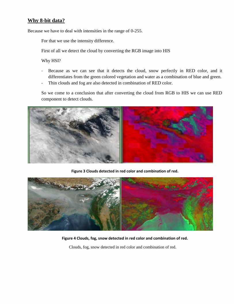
So we come to a conclusion that after converting the cloud from RGB to HIS we can use RED

component to detect clouds.

Figure 3 Clouds detected in red color and combination of red.

Figure 4 Clouds, fog, snow detected in red color and combination of red.

Clouds, fog, snow detected in red color and combination of red.

Thresholding

Now we apply thresholding to differentiate clouds from other regions [2].

Why thresholding?

Because we do not want to detect the edges, we want to detect the whole area pixel by pixel and that is

possible through thresholding.

Threshold Details

Standard Deviation

N

xx

2)(

Where,

=the standard deviation

x =each value in the population(total values)

x =the mean of the values

N =the number of values(the population)

For calculating mean,

x =i

yni

i

i

0

Where,

x =mean

y(pixel intensity)[0,255]

n=number of pixels

Median For calculating median

T=2

maxmin

Where,

T=threshold

min=minimum intensity of pixel

max=maximum intensity of pixel

Limitations:

The major problem with thresholding is that we consider only the intensity, not any

Relationships between the pixels. There is no guarantee that the pixels identified by

thresholding process are contiguous.

The problem is also reflected in result. This algorithm cannot detect ultra thin clouds and light

fog. If the threshold value is decreased so other object like sand and soil is detected because the

intensity of thin clouds, fog and sand is nearly same.

Results:

Threshold

Standard

Deviation

Median

Table 1 Visual comparison of different threshold

Histogram Equalization

Reasons:

It gives contrast between different objects like clouds, water, snow, vegetation, soil, sand etc.

The intensity of cloud and snow is high compare to vegetation, water, soil and sand. After

applying histogram equalization it gives contrast between above objects. Clouds and snow has

high contrast, So it is easy to detect the clouds after applying threshold.

In other words, we can say that Histogram equalization works as filter.

Calculations:

Consider a discrete grey scale image {x} and let ni be the number of occurrences of gray level i. The

probability of an occurrence of a pixel of level i in the image is

Lin

nixpiP i

x 0,)()(

L being the total number of gray levels in the image (typically 256), n being the total number of pixels in

the image, and )(ipx being in fact the image's histogram for pixel value i, normalized to [0,1].

Let us also define the cumulative distribution function corresponding to px as

)()(0

jpicdfi

j

xx

Which is also the image's accumulated normalized histogram.

We would like to create a transformation of the form y = T(x) to produce a new image {y}, with a flat

histogram. Such an image would have a linearized CDF across the value range, i.e.

iKicdf y )(

For some constant K. The properties of the CDF allow us to perform such a transform (see Inverse

distribution function); it is defined as

)()( kcdfkTy x

Where k is in the range [0,L). Notice that T maps the levels into the range [0,1], since we used a

normalized histogram of {x}. In order to map the values back into their original range, the following

simple transformation needs to be applied on the result:

}min{})min{}(max{*' xxxyy

In below example L belongs to [0,255].

Because grey scale image has 8 –bit depth

)1(*

)*(

)()(

min

min LcdfNM

cdfvcdfroundvh

Where cdfmin is the minimum non-zero value of the cumulative distribution function (in this case 1), M ×

N gives the image's number of pixels.

M=width and N=height

Limitations:

Histogram equalization can produce undesirable effects when it is applied on low color depth.

It works based on global threshold value.

The problem is also reflected in the result. In some images the intensity of shadow of object, the

thin clouds and sand will map into the one class when applying equalization operation. So it is

difficult to distinguish thin cloud in image.

Results:

Algorithm

Histogram

Equalization

Table 2 Visual result of histogram equalization

Otsu Clustering:

Reasons:

Due to unsatisfactory results from the above two approaches we decided to go for segmentation through

Otsu’s method.

Working

We use Otsu’s method to segment the input photograph into candidate cloud regions and non-

cloud regions, which can receive a coarse cloud detection result.

Otsu’s method assumes that the photograph to be thresholded contains two classes of pixels or a

bimodal histogram (for example, foreground and background) and then calculates the optimal

threshold separating those two classes so that their interclass variance is maximum.

Algorithm:

Algorithm Steps:

1. Compute histogram and probabilities of each intensity level

2. Set up initial )0(i and

)0(i

Where,

)0(i

: Initial probability

)0(i: Initial mean

3. Step through all possible thresholds t=1….. maximum intensity

1. Update i and i

2. Compute )(2 tb

where

)(2 tb : intra class variance

4. Desired threshold corresponds to the maximum )(2 tb

5. You can compute two maxima (and two corresponding thresholds). )(2

1 tb is the greater max

and )(2

2 tb is the greater or equal maximum

Where,

)(2

1 tb: Class 1 variance

)(2

2 tb: Class 2 variance

6. Desired threshold = 2

21 ThresholdThreshold

Results:

Algorithm

OTSU

clustering

Table 3 Visual result of Otsu clustering

Limitations:

The method does not work well with variable illumination.

Above drawbacks also reflect in results, algorithm does not detect thin clouds and light fog.

References:

1. Shrivastava, P. "Cloud Detection with MATLAB." Journal of Engineering Science and

Technology Review 6, no. 1 (2013): 68-71.

2. Jedlovec, Gary J., and Kevin Laws. "Operational cloud detection in GOES imagery." In 11th

conference on Satellite Meteorology and Oceanography, vol. 357. Madison: Univ of WI,

Madison, 2001.