algorithm and architecture for simultaneous
TRANSCRIPT

Algorithm and Architecture for Simultaneous Diagonalization of Matrices Applied to Subspace-Based Speech Enhancement
Pavel Sinha
A Thesis
in
The Department
of
Electrical and Computer Engineering
Presented in Partial Fulfillment of the Requirements for the Degree of Master of Applied Science at
Concordia University, Montreal, Quebec, Canada
April 2008
© Pavel Sinha, 2008

1*1 Library and Archives Canada
Published Heritage Branch
395 Wellington Street Ottawa ON K1A0N4 Canada
Bibliotheque et Archives Canada
Direction du Patrimoine de I'edition
395, rue Wellington Ottawa ON K1A0N4 Canada
Your file Votre reference ISBN: 978-0-494-40897-1 Our file Notre reference ISBN: 978-0-494-40897-1
NOTICE: The author has granted a nonexclusive license allowing Library and Archives Canada to reproduce, publish, archive, preserve, conserve, communicate to the public by telecommunication or on the Internet, loan, distribute and sell theses worldwide, for commercial or noncommercial purposes, in microform, paper, electronic and/or any other formats.
AVIS: L'auteur a accorde une licence non exclusive permettant a la Bibliotheque et Archives Canada de reproduire, publier, archiver, sauvegarder, conserver, transmettre au public par telecommunication ou par Plntemet, prefer, distribuer et vendre des theses partout dans le monde, a des fins commerciales ou autres, sur support microforme, papier, electronique et/ou autres formats.
The author retains copyright ownership and moral rights in this thesis. Neither the thesis nor substantial extracts from it may be printed or otherwise reproduced without the author's permission.
L'auteur conserve la propriete du droit d'auteur et des droits moraux qui protege cette these. Ni la these ni des extraits substantiels de celle-ci ne doivent etre imprimes ou autrement reproduits sans son autorisation.
In compliance with the Canadian Privacy Act some supporting forms may have been removed from this thesis.
Conformement a la loi canadienne sur la protection de la vie privee, quelques formulaires secondaires ont ete enleves de cette these.
While these forms may be included in the document page count, their removal does not represent any loss of content from the thesis.
Canada
Bien que ces formulaires aient inclus dans la pagination, il n'y aura aucun contenu manquant.
ABSTRACT
Algorithm and Architecture for Simultaneous
Diagonalization of Matrices applied to Subspace based
Speech Enhancement
Pavel Sinha
This thesis presents algorithm and architecture for simultaneous diagonalization of
matrices. As an example, a subspace-based speech enhancement problem is considered,
where in the covariance matrices of the speech and noise are diagonalized
simultaneously. In order to compare the system performance of the proposed algorithm,
objective measurements of speech enhancement is shown in terms of the signal to noise
ratio and mean bark spectral distortion at various noise levels.
In addition, an innovative subband analysis technique for subspace-based time-
domain constrained speech enhancement technique is proposed. The proposed technique
analyses the signal in its subbands to build accurate estimates of the covariance matrices
of speech and noise, exploiting the inherent low varying characteristics of speech and
noise signals in narrow bands. The subband approach also decreases the computation
time by reducing the order of the matrices to be simultaneously diagonalized. Simulation
results indicate that the proposed technique performs well under extreme low signal-to-
noise-ratio conditions.
iii

Further, an architecture is proposed to implement the simultaneous diagonalization
scheme. The architecture is implemented on an FPGA primarily to compare the
performance measures on hardware and the feasibility of the speech enhancement
algorithm in terms of resource utilization, throughput, etc. A Xilinx FPGA is targeted for
implementation. FPGA resource utilization re-enforces on the practicability of the design.
Also a projection of the design feasibility for an ASIC implementation in terms of
transistor count only is included.
iv

Acknowledgement
I would like to take this opportunity in expressing my sincere gratitude to my mentor and
research advisor Professor M.N.S. Swamy for his guidance, encouragement and support
throughout my graduate studies. It has been a great pleasure working with him.
I gratefully acknowledge Dr. P.K Meher, faculty of Nanyang Technological
University, Singapore, for his advice from time to time.
I extend my whole-hearted gratitude to my family for their encouragement and
support, without which it could have been impossible to finish this work. Finally, I would
like to thank my friends for their valuable advice and warm support.
Pavel Sinha, April 2008
v

I dedicate this work to my grandfather, late Shri Mrighendra Bhusan Sinha
and I hope this work has made him proud of me...

Table of Contents
List of Figures x
List of Tables xiv
List of Symbols xv
List of Abbreviations xvi
Chapter 1 : Introduction 1
1.1 Introduction and Motivation 1
1.2 Scope and Thesis Organization 5
Chapter 2 : Hardware-Efficient Matrix Diagonalization 7
2.1 Review of Matrix diagonalization using Jacobi Technique 7
2.2 CORDIC Algorithm: A Review 13
2.3 Simultaneous Diagonalization of Matrices using CORDIC 16
2.3.1 GainGR 20
2.3.2 Summary of the Algorithm 21
2.4 Error Analysis of the CORDIC Based Diagonalization Engine 22
2.4.1 Mean Off Diagonal Error of the Diagonalized Matrix 22
2.4.2 Mean Reconstruction Error of the Constructed Matrices 25
2.5 Summary 27
Chapter 3 : Speech Enhancement 28
3.1. Review of Subspace Based Speech Enhancement Technique 28
3.1.1 Optimal Subspace Filter for Speech Enhancement 30
3.1.2 Estimating the Lagrange Parameter n 33
3.2. Frequency Sub-Band Processing into Subspace based Speech Enhancement 35
3.2.1. Theory of Frequency Sub-Band Processing 36
vii
3.2.2. Justifying the Need for Sub-Band Processing 39
3.3. Objective Performance Measures and Experimental Results 40
3.3.1. Signal to Noise Ratio (SNR) 40
3.3.2. Segmental SNR (SSNR): 41
3.3.3. The Itakura Saito distance (ISD) Measure: 42
3.3.4. Modified Bark Spectral Distortion (MBSD) Measure: 42
3.3.5. Experimental Results and Discussion 44
3.4. Summary 49
Chapter 4 : Multiplier-Free Architecture for the Proposed Simultaneous
Diagonalization Scheme 50
4.1. Architecture of the Eigen Domain Filter 51
4.1.1. CORDIC Architecture of a Single Processing Element 52
4.1.2. Multiply and Accumulate (MAC) Unit 55
4.1.3. The Autocorrelation Unit 57
4.1.4. Eigen-Domain Filter Gain Calculation Unit 62
4.1.5. Jacobi Pair (P, Q) Generation Unit 64
4.2. Memory Architecture 66
4.2.1. DMSM Memory Cell 67
4.2.2. DMSM Memory Organization 68
4.3. Memory Controller FSM Design 70
4.3.1. Top Memory Controller 72
4.3.2. Memory Controller Mode-I 75
4.3.3. Memory Controller Mode-II 75
4.3.4. Memory Controller Mode III 76
4.3.5. Memory Controller Mode IV 77
4.4. Parallel Architecture of the Diagonalization Unit 79
4.5. The Master Controller 82
4.5.1. TOP Controller Design 82
via

4.6. Frequency-Subband based Speech Enhancement Processor 82
4.7. Summary 87
Chapter 5 : Results & Discussion 88
5.1 System Level Comparison of Speech Enhancement 88
5.2 Hardware Implementation Results of Subspace based Speech Enhancement 91
5.2.1 FPGA Resource Utilization 91
5.2.2 Throughput Analysis 92
5.2.3 Number of Logic Elements 94
5.2.4 Transistor Count for ASIC Implementation 95
5.2.5 Design Specifications 96
5.3 Implementation results of the frequency subband CORDIC- based subspace
speech enhancement 102
5.3.1 FPGA Resource Utilization 102
5.3.2 Throughput Analysis 102
5.3.3 Number of Logic Elements 103
5.3.4 Transistor Count for ASIC Implementation 104
5.3.5 Design Specifications 109
5.4 Summary 109
Chapter 6 : Conclusion I l l
6.1. Conclusion and Thesis Summary 111
6.2. Future Work 113
References 114
Appendix A: 124
ix
List of Figures
Figure 2.1. Mean Off diagonal error of the diagonalized matrix for varying matrix
sizes, for 100 pairs of randomly generated symmetric matrices, (a) for
varying CORDIC rotations and (b) for varying Jacobi iterations 24
Figure 2.2. Mean reconstruction error of the constructed matrices from the
calculated eigen-vectors and eigen-values for varying matrix sizes, for
100 pairs of randomly generated symmetric matrices, (a) for varying
CORDIC rotations and (b) is for varying Jacobi iteration 26
Figure 3.1 System Overview 36
Figure 3.2: Spectrogram of a typical clean speech of a TIMIT sentence 45
Figure 3.3: Comparison of the spectrogram of speech in Figure 2 corrupted by the
car noise at -10 db SNR with that of the speech after the proposed
filtering 45
Figure 3.4: Comparative performance for car noise at various SNR in terms of
Itakura distance, segmental SNR, and MBSD measures for 20 TIMIT
sentences produces by 10 male and 10 female speakers 46
Figure 3.5: Comparative performance for babble noise at various SNR in terms of
Itakora distanc, segmental SNR, and MBSD measure for 20 TIMIT
sentences produces by 10 male and 10 female speakers 47
Figure 3.6: Comparative performance for F16 cockpit noise at various SNR in terms
of Itakora distance, segmental SNR and MBSD measure for 20 TIMIT
sentences produces by 10 male and 10 female speakers 48
x
Figure 4.1: CORDIC architecture of a single PE 53
Figure 4.2: PE Controller I/O block diagram 53
Figure 4.3: Timing diagram of only the major I/O signals in a PE during operation 56
Figure 4.4: The FSM of the PE master controller 56
Figure 4.5: The FSM of the PE sign controller 57
Figure 4.6: The FSM of the PE execution controller 58
Figure 4.7: MAC unit RTL for serial matrix multiplication 59
Figure 4.8: The autocorrelation unit 59
Figure 4.9: The FSM of the autocorrelation controller 62
Figure 4.10: The eigen-domain filter (with variable SNR) 63
Figure 4.11: The register transfer level (RTL) diagram of the eigen-domain filter 63
Figure 4.12: The FSM of the divide controller 65
Figure 4.13: LUT based serial (P, 0-pair generation 66
Figure 4.14: LUT based parallel (P, 0-pair generation 66
Figure 4.15: Dual port multiple row/column shift memory (DMSM) I/O block
diagram 68
Figure 4.16: DMSM cell I/O block diagram 68
Figure 4.17: The internal structure of the DMSM 70
Figure 4.18: DMSM (dual port multiple row/column shift memory) controller I/O
block diagram 71
Figure 4.19: State transition diagram of the Top memory controller 73
Figure 4.20: Memory controller Mode-1 74
Figure 4.21: Memory controller Mode-II 76
xi
Figure 4.22: Memory controller Mode-Ill 78
Figure 4.23: Memory controller Mode-IV 79
Figure 4.24: Parallel implementation of N/2 Jacobi rotations for a total of R
CORDIC iterations 81
Figure 4.25: Hierarchy of the speech processor controllers 83
Figure 4.26: TOP Controller 84
Figure 4.27: Frequency-Subband Speech processor 85
Figure 4.28: Frequency-Subband Speech Processor 86
Figure 5.1: Comparison of the proposed (SJR) diagonalization vs. Matlab
(Cholesky) factorization (SSF) for factory noise in terms of segmental
SNR and mean MBSD measures of 20 TIMIT sentences from a female
speaker 89
Figure 5.2: Throughput vs. the number of parallel PEs used for different window
sizes 98
Figure 5.3: Throughput vs. the number of parallel PEs used for different clock rates 98
Figure 5.4: Number of hardware elements required as a function of the window
size 99
Figure 5.5: Total number of registers required as a function of the number of
parallel PEs used, for varying window sizes 99
Figure 5.6: Transistor count analysis excluding the data memory, as a function of
the number of parallel PEs used, for varying window sizes 100
XII
Figure 5.7: Transistor count analysis excluding the data memory, as a function of
the number of parallel PEs used, for varying number of parallel
CORDIC elements used 100
Figure 5.8: Throughput results as a function of the number of filter banks for
various number of parallel PEs 105
Figure 5.9: Total number of register as a function of the number of parallel PEs for
various number of filter banks 105
Figure 5.10: Total number of adders used as a function of the number of filter
banks for various number of parallel PEs 106
Figure 5.11: number of hardware elements required as a function of the number of
filter banks 106
Figure 5.12: Transistor count analysis excluding the data memory, as a function of
the number of filter banks used, for varying number of PE elements
used 107
Figure 5.13: Transistor count analysis excluding the data memory, as a function of
the number of filter banks used, for varying number of CORDIC
elements used 107
Figure A-1.Comparison of the eigen-values of (a) matrix A'l and Al'_matlab (b)
matrix A'2and A2'_matlab 127
Figure A-2.Comparing the mesh plots of the diagonalized matrices (a) matrix A'l
and (b) matrix Al'_matlab 127
Figure A-3. Comparing the mesh plots of the diagonalized matrices (a) matrix A'2
and (b) matrix A2'_matlab 128
xiii

List of Tables
Table 5-1: HDL Synthesis report of a Single PE 93
Table 5-2: Timing Summary of a Single PE 93
Table 5-3: FPGA Resource Utilization of a Single PE 94
Table 5-4: Transistor count for various digital logic functions 97
Table 5-5: Design Specifications: Speech enhancement on FPGA 101
Table 5-6: FPGA Resources for 16 bit data path 103
Table 5-7: FPGA Timing Summary for 16 bit datapath 103
Table 5-8 Design Specifications: Subband based speech enhancement on FPGA 108
XIV
List of Symbols
Ad A diagonal matrix that approximates Rd
£d
£x
¥
h A
M
a(i,j)
add/sub
(c,s)
Ok
E{}
EE
Ex
FMAX
GR
"opt
J(p. q. 6)
MHz
MUX
Myp
ns
Rd
Rx
tr{)
V
Kesidual noise Speech distortion
KxMmatrix with rank M(M< K)
ith Eigen-value
Eigen-value matrix
Lagrange parameter
Element in a matrix (th row and/'' column)
Addition or subtraction
Cosine and sine pair elements in a Jacobi matrix
Clock signal
Expectation operator
Error signal energy
Signal energy
Maximum clock frequency
CORDIC gain after R iterations
Optimal statistical filter matrix
Jacobi matrix with elements in p'h row and qth co
Mega-Hertz
Multiplexer
Multiplication
Nano second
Covariant matrix of noise d
Covariant matrix of clean speech X
Trace operator
Eigen-vector matrix
XV
List of Abbreviations
ASIC
BSD
CORDIC
DMSM
EVD
FDC
FIFO
FPGA
FSM
ICA
ISD
KLT
LUT
MAC
MBSD
PCA
PE
QSVD
RTL
SNR
SSNR
SVD
TDC
VHDL
VLSI
WLS
Application specific integrated circuits
Bark spectral distortion
Coordinate rotation digital computer
Dual port multiple row/column shift memory
Eigen-value decomposition
Frequency domain constraint
First in first out
Field programmable gate array
Finite state machine
Independent component analysis
Itakora-Saito distance
Karhunen Loeve transform
Look-Up table
Multiply and accumulate
Mean bark spectral distortion
Principal component analysis
Processing element
Quotient Singular Value Decomposition
Register transfer level
Signal to noise ratio
Segmental signal to noise ratio
Singular value decomposition
Time domain constrain
Very high speed integrated circuit, hardware description language
Very large scale integrated circuit
Weighted least squared
XVI

Chapter 1 : Introduction
1.1 Introduction and Motivation
From the beginning of human civilization, speech has been the primary and most
important medium for communication and exchange of ideas and thoughts among
individuals. Even in the 21st century, speech remains to be the primary medium of
communication in our day to day life [1] [2], aviation, military [3], distress calls, etc.
Enhancement of degraded speech over communication channels readily finds its
application in aircraft, mobile, military and commercial communications and in aids for
the handicapped. Applications include both speech over noisy transmission channels (e.g.
cellular telephony) and speech produced in noisy environments (e.g. in vehicles or
telephone booths) [2].
The objective of the speech enhancement algorithms vary widely from noise level
reduction, increased intelligibility, decreasing auditory fatigue, reducing transmission
data rates, etc. In recent years, numerous speech enhancement algorithms have been
proposed. Statistical signal processing has become very popular in speech enhancement
algorithms. The problem of approximate eigen-domain decomposition and joint
diagonalization of a set of matrices has become instrumental in numerous statistical
signal processing applications [4], [5], [6] involving principle component analysis (PCA)
[7], blind beam-forming [8], blind source separation (BSS) [9], frequency estimate [10],
1

Independent component analysis (ICA) [11] and de-noising techniques for single/multi
dimensional signal processing [12]. As their distinguished feature, these methods seek to
extract the desired information about the signal and noise by first estimating, either in
part or full, the eigen-values using the eigen-value decomposition (EVD) technique.
However, the popularity is limited due to its intense computational complexity.
Moreover, the computational requirement of the eigen-domain decomposition increases
exponentially with the matrix size [5], [6], [13].
Another statistical signal processing approach is the projection approximation
subspace tracking. In his work [5], the author has interpreted the signal subspace as the
solution of a projection-like unconstrained minimization problem. The recursive least
square technique has been applied by making appropriate projection approximation.
However, its performance is not well accepted for sensitive applications, where an
accurate estimate of the subspace is necessary [14]. Specially under heavy noise
conditions, the least square algorithm fails to track the subspace. An adaptive Jacobi
method for parallel implementation of singular value decomposition (SVD) has been
given by Shen-Fu Hsiao [13]. A modified parallel adaptive Jacobi method to diagonalize
a symmetric matrix has been presented in [6]. Later, the subspace tracking was addressed
by Benoit and Qing-Guang [15], [16] by an efficient updating scheme of plane rotation-
based eigen-value decomposition (EVD), using a parametric perturbation approach. In a
recent work by Xi-Lin Li and Xian-Da Zhang [17], a non-orthogonal joint
diagonalization method has been presented; it is an approximate non-orthogonal joint
diagonalization technique and analyzes the inefficiency of the weighted least-squares
(WLS) approach used by Wax [18].
2

With the development of eigen-domain estimation algorithms, subspace based
techniques have emerged as a promising statistical tool. Subspace-based speech
enhancement techniques have been designed to reduce noise levels in noisy speech
signals and at the same time minimize speech distortions. The mathematical formulation
leads to a constraint minimization problem, which is readily solved by using the method
of Lagrange multipliers resulting in an optimal statistical speech enhancement filter. The
use of the subspace approach was pioneered by Ephraim and Van Trees [19], who
proposed the optimal estimator for white noise that was later extended to the case of
coloured noise by Hu and Loizou [20]. The original subspace enhancement scheme was
developed in time and frequency domains, leading to the time domain constraint (TDC)
and frequency domain constraint (FDC) versions of the algorithm. The performance of
the subspace algorithm mainly depends on two steps, namely, the accurate estimation of
the noise and noisy speech covariance matrices and the shaping of the residual noise
terms. The former leads to reduced speech distortions, while the latter improves the
quality of the enhanced speech by exploiting the perceptual properties of hearing. Much
of the contemporary research has focussed on developing robust and novel techniques to
obtain better estimates and perform suitable noise shaping.
In the subspace approach, the distortions in the enhanced speech signal are evident in
low SNR conditions. This is due to the inaccurate estimation of the speech and noise
covariance matrices. The poor estimation stems from the fact that the noise and noisy
speech subspaces exhibit an increasing overlap with decreasing SNR [19]. In particular, it
has been identified that the poor estimation of the noise and speech spectra leads to
annoying artefacts such as the "musical noise" in the enhanced speech. Musical noise is a
3
result of spectral spikes occurring at random frequencies caused due to large variance
estimation of noise and speech signals [19]. While masking the residual error mitigates
the effects of the annoying artefacts, it has been pointed out that a more accurate
estimation of the SNR may be beneficial in removing the musical noise. Therefore,
accurate spectral estimation has been recognized as a key step towards robust
performance, and many techniques, such as the multi-taper and Blackman-Tukey, have
been developed for this purpose [21], [22]. Also, the use of wavelet thresholding
technique, such as the SURE, results in more accurate spectral estimates and eliminates
the musical noise [23], [21].
However, in most of the work presented so far, very little effort has been made to
address the problem of real-time computation from a hardware point of view. Most of
these algorithms have implementation issues in real-time. The bottle neck is in achieving
higher throughput rates when implemented on VLSI, followed by the hardware
complexity and the static power dissipation [24]. Most of the modern state of the art DSP
algorithms involving intense statistical estimation become impractical for VLSI
realization or for real-time realizations on high performance system platforms. This
brings in the need for reducing hardware complexity of the algorithms being developed.
With the emerging need for eigen-domain estimations and statistical filters in most of the
real-time signal processing applications, complexity increases exponentially with the
window size used in the algorithm.
The requirement for executing computationally-intensive functions at hardware speed
can only be satisfied by the emerging application specific integrated circuits (ASICs).
Even though ASICs offer highest possible performance at lowest silicon cost, they suffer
4
from inflexibility. Besides, if a particular application needs a large number of functions to
be executed in real-time, then a large number of ASIC chips will be required, and thus, is
not cost effective [25]. Field programmable gate arrays (FPGA) on the other hand are
high performance programmable hardware that allows flexibility and reconfigurability
for realizing a diverse class of functions. Research in the area of mapping complex DSP
algorithms onto reconfigurable FPGA has revealed that the FPGAs are adequate and best
suited for mapping most of the computationally intensive applications, due to their
efficient static ram-based LUT designs offering an optimum cost-performance trade-off
[26].
1.2 Scope and Thesis Organization
The above discussion provides sufficient background to establish the fact that statistical
signal processing is highly computationally intensive. Emerging speech enhancement
algorithms fully rely on statistical computations, such as eigen-domain estimations.
Hardware implementation issues also limit the application of such algorithms in real
time. In this thesis, the problem of simultaneous approximate diagonalization of multiple
matrices is studied. As an application, the problem of subspace-based speech
enhancement technique is considered, while keeping in mind the implementation issues
of modern day VLSI circuits. A solution to the problem of achieving high throughput and
reduced computation cost is also addressed through an innovative frequency subband
5

processing. The subband approach exploits the inherent low variance of the speech and
noise signals in a limited frequency region as opposed to using the full band.
This thesis consists of six chapters. Chapter 2 mainly focuses on the joint
diagonalization of matrices. It gives an insight to the Jacobi-based matrix diagonalization
technique. It also provides a review of the CORDIC algorithm. The later part of the
chapter presents an innovative technique to approximately diagonalize a pair of
symmetric matrices simultaneously, based on the extension of the Jacobi diagonalization
technique combined with the CORDIC implementation scheme. This results in an
efficient multiplier-free hardware implementation of the algorithm, and has been shown
later in Chapter 4. Chapter 3 focuses on a time domain constrained subspace-based
speech enhancement algorithm. Starting with a brief discussion on speech enhancement,
this chapter also extends the time domain constrained algorithm to an efficient frequency
subband speech processing technique for improved performance. Chapter 4 deals with the
architecture that supports the CORDIC based Jacobi core for simultaneous
diagonalization of matrices used in speech enhancement. The area-optimized architecture
for the sub-band sub-space optimal filter is also presented. Chapter 5 then discusses the
results and comparisons that justify the hardware implementation. Later, the overall
system performance of the speech enhancement architecture is discussed. The FPGA
resource utilization of the architecture is also presented. Finally, Chapter 6 contains some
conclusions and focuses on some of the future work that could be carried out.
6
Chapter 2 : Hardware-Efficient Matrix
Diagonalization
Matrix diagonalization is equivalent to transforming the underlying system of equations
represented by the matrix, into a special set of coordinate axes in which the matrix takes
this canonical form. The process of diagonalization essentially consists of computing the
eigen-values, which are the diagonal entries of the diagonalized matrix while the
eigenvectors, also known as the characteristic vectors, make up the new set of axes
corresponding to the diagonal matrix. This chapter briefly presents a review of the
Jacobi-based diagonalization algorithm followed by a review of the CORDIC-based
computation technique. The later part of the chapter presents an innovative and simple
extension of the Jacobi technique to diagonalize multiple symmetric matrices using the
CORDIC algorithm.
2.1 Review of Matrix diagonalization using Jacobi Technique
The Jacobi-based matrix diagonalization algorithm is a numerical technique for
calculating the eigen-values and eigen-vectors of a real symmetric matrix. The method is
named after the German mathematician, Carl Gustav Jakob Jacobi. Jacobi method has
attracted attention for applications dealing with eigen-values of symmetric matrices,
since they have an inherent unique property that facilitates parallel execution of the
7
algorithm. It works by performing a series of orthogonal similar transforms. The key
property in achieving the diagonalized matrix lies in the fact that each of these orthogonal
transform produces an approximate diagonalized matrix, which is "approximately more
diagonal" than its predecessor. Eventually, when the off-diagonals are small enough to be
declared zero, the matrix is considered to be diagonalized.
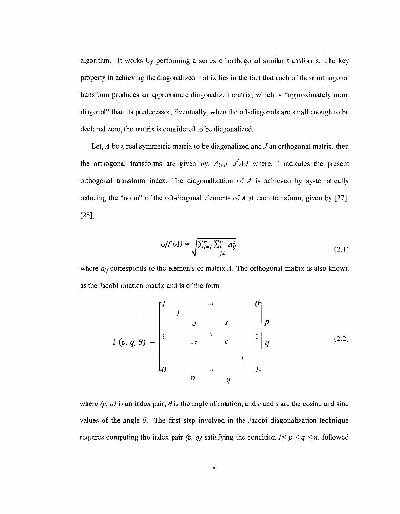
Let, A be a real symmetric matrix to be diagonalized and J an orthogonal matrix, then
the orthogonal transforms are given by, Ai+i<r-JTAjJ where, i indicates the present
orthogonal transform index. The diagonalization of A is achieved by systematically
reducing the "norm" of the off-diagonal elements of A at each transform, given by [27],
[28],
off(A)= \LUY?Ma\ m
(2.1)
where fly corresponds to the elements of matrix A. The orthogonal matrix is also known
as the Jacobi rotation matrix and is of the form
r7
J (p, q, 6) = -s
0
(h
P
q (2.2)
where (p, q) is an index pair, 0 is the angle of rotation, and c and s are the cosine and sine
values of the angle 0. The first step involved in the Jacobi diagonalization technique
requires computing the index pair (p, q) satisfying the condition l<p <q <n, followed
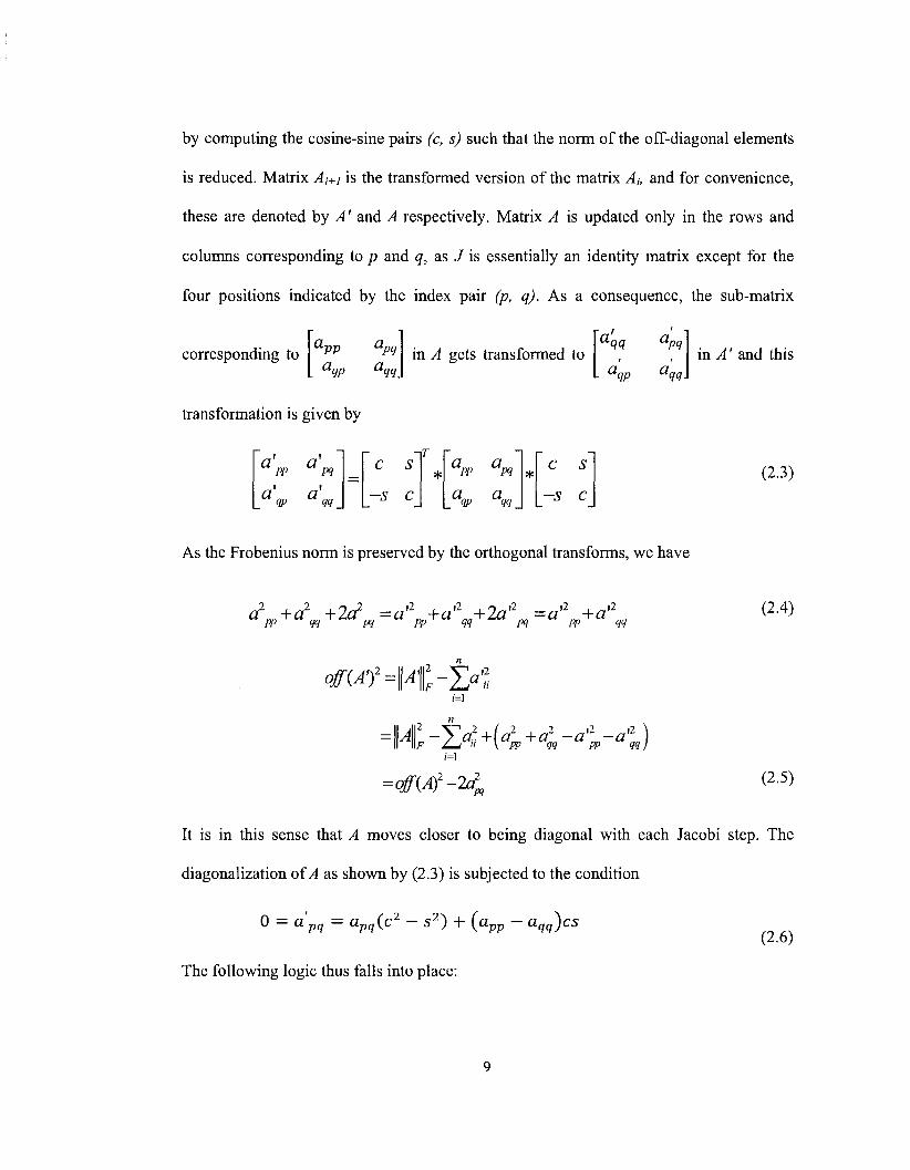
by computing the cosine-sine pairs (c, s) such that the norm of the off-diagonal elements
is reduced. Matrix Ai+i is the transformed version of the matrix At, and for convenience,
these are denoted by A' and A respectively. Matrix A is updated only in the rows and
columns corresponding to p and q, as J is essentially an identity matrix except for the
four positions indicated by the index pair (p, q). As a consequence, the sub-matrix
Q-pp apq
®qp &qq corresponding to
transformation is given by
in A gets transformed to a qq
a,
a, pq
qp a. qq
in A' and this
a' PP
a' IP
a' pq
a' m_
c
-s
s
c
T
* a a pp m
a a IP W
c s
-s c
As the Frobenius norm is preserved by the orthogonal transforms, we have
(2.3)
o2 +d +202 =a'2 +aa +2aa =aa +aa pp w m PP m m PP <?<?
off(Af=\\AfF-^l 1=1
= \\4-fa2+(a2 +a2 -a'2 -a'2 ) II \\F L~in \ PP m PP qq)
=off(A)2-2al
i=i
.2 ", 2
pq
(2.4)
(2.5)
It is in this sense that A moves closer to being diagonal with each Jacobi step. The
diagonalization of A as shown by (2.3) is subjected to the condition
U CL pq &pq\C S J ~r yO-pp ®-qq)CS (2.6)
The following logic thus falls into place:
9
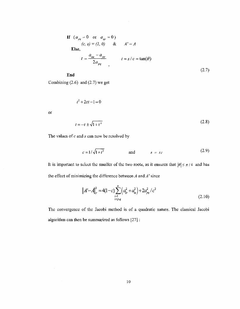
If (apq=0 or a„=0)
(c,s) = (l,0) & A' = A Else,
r=aqq a"p t = s/c = Um(0) 2aP, .
(2.7) End
Combining (2.6) and (2.7) we get
t2+2vt-\ = 0
or
The values of c and s can now be resolved by
c = \/Jl + t2 and 5 = /c (2'9)
It is important to select the smaller of the two roots, as it ensures that \e\ < n 14 and has
the effect of minimizing the difference between A and A' since
;j,« (2-10)
The convergence of the Jacobi method is of a quadratic nature. The classical Jacobi
algorithm can then be summarized as follows [27] :
10
a pi
= max,v.
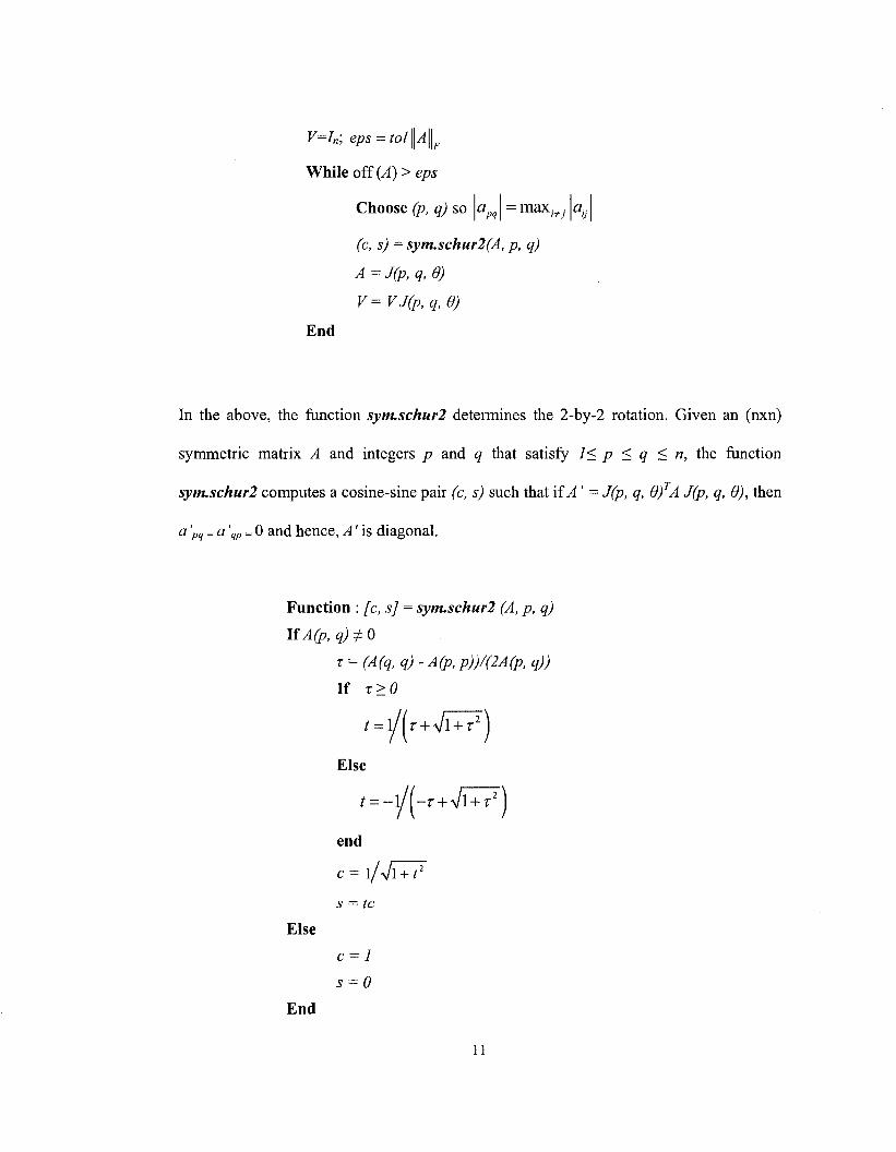
V—I„; eps = tolftAft
While off (A)>eps
Choose (p, q) so
(c, s) = sym.schur2(A, p, q)
A=J(p,q,0)
V=VJ(p,q,6)
End
In the above, the function sym.schur2 determines the 2-by-2 rotation. Given an (nxn)
symmetric matrix A and integers p and q that satisfy 1< p < q < n, the function
sym.schur2 computes a cosine-sine pair (c, s) such that if A ' = J(p, q, 0)TA J(p, q, 6), then
a'Pq = a 'gp = 0 and hence, A' is diagonal.
Function : [c, s] = sym.schur2 (A, p, q)
If A(p, q)^0
x = (A(q,q)-A(p,p))/(2A(p,q))
If x>0
t =
e
t =
I
-1
-)
(r + Vl + r2)
/ ( - r + Vl + r 1 - i M c = 1/V1 + ^2
Else
End
s = tc
c = 1
11
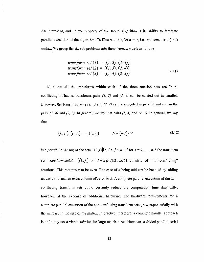
An interesting and unique property of the Jacobi algorithm is its ability to facilitate
parallel execution of the algorithm. To illustrate this, let n = 4, i.e., we consider a (4x4)
matrix. We group the six sub problems into three transform sets as follows:
transform, set (1) = {{1, 2), (3, 4)}
transform, set (2) = {(7, 3), (2, 4)}
transform, set (3) = {(7, 4), (2, 3)} ( 2 - 1 1 )
Note that all the transforms within each of the three rotation sets are "non-
conflicting". That is, transforms pairs (1, 2) and (3, 4) can be carried out in parallel.
Likewise, the transform pairs (1, 3) and (2, 4) can be executed in parallel and so can the
pairs (1, 4) and (2, 3). In general, we say that pairs (1, 4) and (2, 3). In general, we say
that
(hJt).(hJ1).:..(inJn) N={n-l)n/2 (2.12)
is ^parallel ordering of the sets {(*,./) |l <i< j <n) if for s = 1, ... , n-1 the transform
set transform.set(s) = {{ir,j ) :r = 1 +n (s-l)/2 : ns/2] consists of "non-conflicting"
rotations. This requires n to be even. The case of n being odd can be handled by adding
an extra row and an extra column of zeros to A. A complete parallel execution of the non-
conflicting transform sets could certainly reduce the computation time drastically,
however, at the expense of additional hardware. The hardware requirements for a
complete parallel execution of the non-conflicting transform sets grow exponentially with
the increase in the size of the matrix. In practice, therefore, a complete parallel approach
is definitely not a viable solution for large matrix sizes. However, a folded parallel-serial
12

approach is usually an attractive choice, since it maintains a balance between the
hardware cost and the performance [29].
A detailed discussion of error analysis of the Jacobi algorithm is available in [30],
[32]. Wilkinson was the first to perform an error analysis for the Jacobi algorithm for
symmetric matrix diagonalization. Later, a refined error analysis was presented by
Demmel and Veselic in 1992 [31], where he shows that the Jacobi algorithm is more
accurate than the QR factorization algorithm used for matrix diagonalization.
2.2 CORDIC Algorithm: A Review
Digital signal processing has been historically dominated by microprocessors with
enhanced features such as single cycle multiple-accumulate instructions, zero over-head
looping, special addressing modes and bit-reversal techniques. Though the DSP
processors offer low cost and high flexibility, they do not meet the true demands of DSP
tasks. This has led to the development of iterative algorithms that could be mapped well
on to the hardware. With the advancements in reconfigurable computing techniques such
as the FPGAs, hardware-based approaches have become more and more viable than the
traditional software-based approaches [26]. Among these algorithms are a class of shift-
add algorithms for computing a wide range of functions including certain trigonometric
functions, and are collectively known as CORDIC.
CORDIC is an acronym for Coordinate Rotation Digital Computer. The original
work is credited to Jack Voider [33]. Extensions to the CORDIC theory based on the
13

work by John Walther [34] and others provide solutions to a broader class of functions.
These functions are computed with simple extensions to the CORDIC architecture [29].
Though many functions are not strictly computed as in a CORDIC algorithm, they are
often included because of their close similarity.
The problem of real-time solutions for navigation purposes was one of the prime
motivations for the development of the CODIC algorithm. The CORDIC algorithm has
found its way into diverse applications including the 8087 math coprocessor, the HP-35
calculator, radar signal processors and robotics [35]. CORDIC rotation has also been
proposed for computing discrete Fourier, discrete cosine, discrete Hartley and discrete
chirp-z transforms, filtering, singular value decomposition (SVD) and solving linear
system of equations [34], [35], [36], [37] and [38].
Vector rotations are one of the key components for computing the various
trigonometric functions as well as for conversions from polar to rectangular coordinate
system and vice versa. They can also be used for computing vector magnitudes [29] and
as a building block in certain transforms such as the DFT and DCT. The CORDIC
algorithm provides an iterative base for such vector rotations by only shift and adds
operations, thereby being extremely useful for VLSI implementations [35]. The original
algorithm, credited to Voider [33], is basically a series of transforms given by
y
cos# - s i n 0
sin Q cos#
= cos 0 1
tan6>
x
y.
tan 0
1 x
y (2.13)
which rotates a vector in the cartesian plane by an angle 6. So far, nothing is simplified in
terms of the hardware required, as it involves multiplication operations. However, if we
14

can restrict the rotation angle such that tan(6) - ± 2'', the multiplication by the tangent
term is simply reduced to a bunch of shift and addition operations. Any arbitrary angle of
rotation is obtained by a series of rotations, where the decision of the direction of rotation
at the ith stage is governed by the sign of the angle by which the axes are to be rotated.
Thus, (2.13) is simplified to
Xi+\
JM. = Ki I
1
d,2~'
-dt2~r
1
~x
J (2.14)
where
Kt= cos [tan-1 (2" '))=-r=i 1+2--
(1 dt={
for 6 >0
for 9<0
Kj is known as the scaling constant, while dt as the directional bit. The product of AT,-'s is
pre-computed in the system and results in only a constant coefficient multiplication, thus
leading to an efficient VLSI implementation. The product approaches 0.6073 as the
number of iterations tends to infinity. Therefore, the rotation algorithm has a gain, and
the exact gain depends on the number of iterations and obeys the relation
Gain MVTTP
(2.15)
A CORDIC rotation is primarily achieved by a sequence of angle rotations. The angular
values are supplied by a small lookup table (one entry per iteration) or are hardwired,
15

depending on the implementation. The angle accumulator introduces a difference
equation to the CORDIC algorithm, to keep track of the total angle rotated for the given
number of iterations, and is given by
Z^^Zi-dtJan^r) (2.16)
where, Z, stores the angle accumulated at the i'h iteration. Most of the CORDIC functions
are achieved by setting different initial conditions to (2.14) and (2.16) [33], [34], [37].
VLSI implementation of the CORDIC algorithm has also found itself in serial, parallel
and folded semi parallel-serial implementation schemes due to efficient shift and add
functional units. Though the convergence of the CORDIC algorithm is quadratic [27], its
recursive nature hampers the overall system throughput rate.
2.3 Simultaneous Diagonalization of Matrices using CORDIC
This section presents a CORDIC-based scheme to simultaneously diagonalize multiple
symmetric matrices. The Jacobi rotation technique to diagonalize a single matrix [27] is
now extended for the diagonalization of multiple matrices. Let, Aj and A2 be two real
symmetric matrices intended to be simultaneously diagonalized and J an orthogonal
matrix, then the extension of the algorithm is based on performing a sequence of
orthogonal similar update pairs An+i<r-JTA]jJ and A2i+i*—JTA2iJ, where ' j ' indicates the
index of the present orthogonal transform. Each transform has the property that each new
16
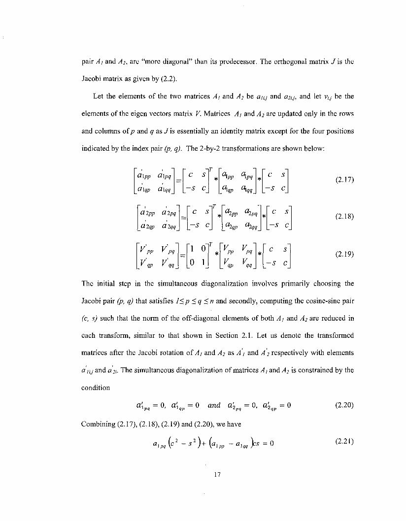
pair Aj and A2, are "more diagonal" than its predecessor. The orthogonal matrix J is the
Jacobi matrix as given by (2.2).
Let the elements of the two matrices Ai and A2 be anj and 02/,;, and let v,,y be the
elements of the eigen vectors matrix V. Matrices A\ and A2 are updated only in the rows
and columns of p and q as J is essentially an identity matrix except for the four positions
indicated by the index pair (p, q). The 2-by-2 transformations are shown below:
&\pp Q \pq 1 1
Cl\qp Q\qq
CI 2pp CI 2pq 1 1
CI 2qp CI 2qq
V pp V pq I I
V qp V qq
C S
-S C
c s
-s c
Q\pp a\pq
a\qp a\qq
fypp fypq
Chqp Chqq
1 0
0 1
IT r V V pp pq
V V qp qq
c s
-s c
c s
-s c
c s
-s c
(2.17)
(2.18)
(2.19)
The initial step in the simultaneous diagonalization involves primarily choosing the
Jacobi pair (p, q) that satisfies l<p <q <n and secondly, computing the cosine-sine pair
(c, s) such that the norm of the off-diagonal elements of both A\ and A2 are reduced in
each transform, similar to that shown in Section 2.1. Let us denote the transformed
matrices after the Jacobi rotation of ^4; and A2 as A) and A 2 respectively with elements
a nj and a 21- The simultaneous diagonalization of matrices A\ and A2 is constrained by the
condition
a[ = 0, a i = 0 and a'2 = 0, a'2 = 0 (2.20)
Combining (2.17), (2.18), (2.19) and (2.20), we have
17
a , (c2 - s2 )+ (a, - a , )cs = 0
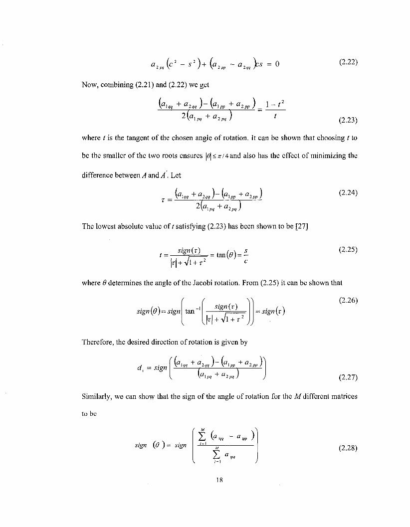
Now, combining (2.21) and (2.22) we get
(2.22)
f (2.23)
where 7 is the tangent of the chosen angle of rotation. It can be shown that choosing t to
be the smaller of the two roots ensures |<9|<;z74and also has the effect of minimizing the
difference between A and A . Let
(«1W + «2<J-(<V + «2;J (2.24) T =
The lowest absolute value of / satisfying (2.23) has been shown to be [27]
t = sign(v)
-| + Vl + r2 = tan(#) =
(2.25)
where 9 determines the angle of the Jacobi rotation. From (2.25) it can be shown that
^ (2.26) r ngn(0) sign\p)- sign
r
tan
v v
sign(x)
H + Vi + X - sign (0
J)
Therefore, the desired direction of rotation is given by
di = sign {a,qq+a2qq)-{a^pp+a2pP)
(2.27)
Similarly, we can show that the sign of the angle of rotation for the M different matrices
to be
f M
sign (d)~ sign Z("
2 a*. \ <=i
(2.28)
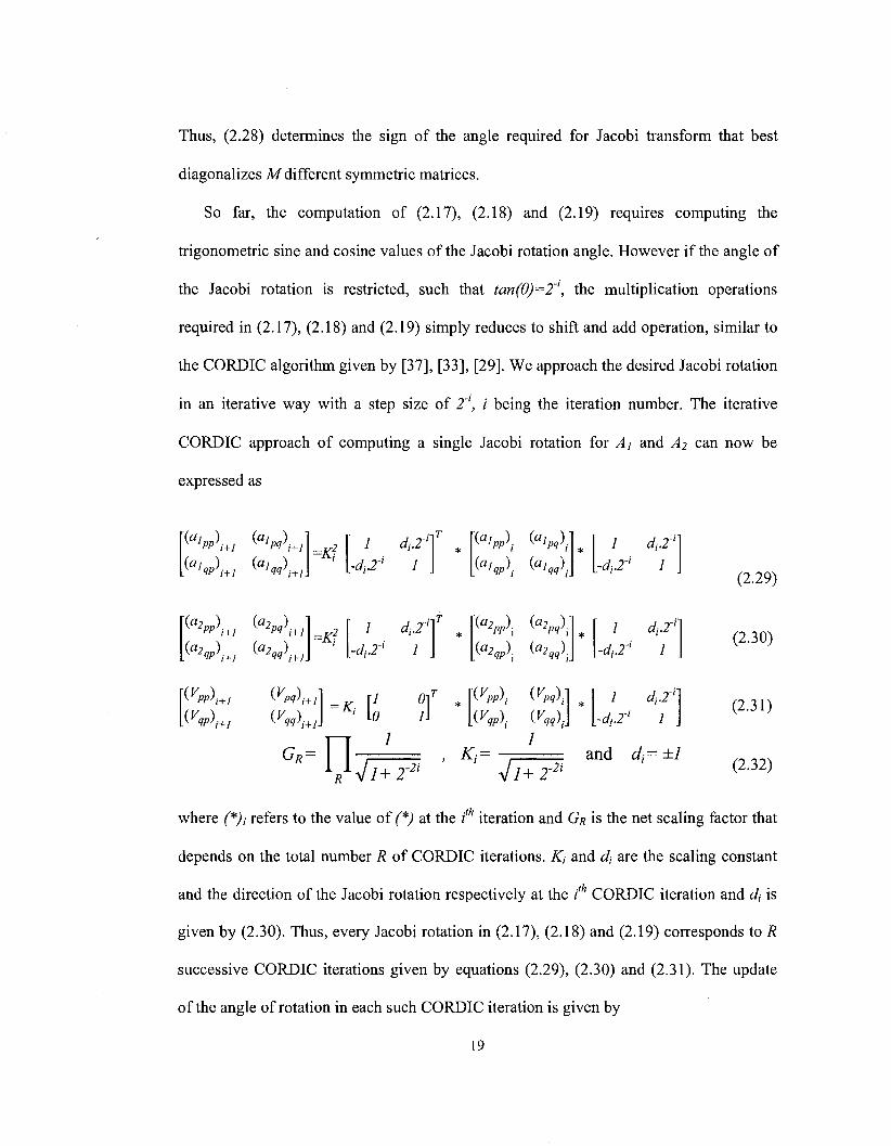
Thus, (2.28) determines the sign of the angle required for Jacobi transform that best
diagonalizes Mdifferent symmetric matrices.
So far, the computation of (2.17), (2.18) and (2.19) requires computing the
trigonometric sine and cosine values of the Jacobi rotation angle. However if the angle of
the Jacobi rotation is restricted, such that tan(9)=2~', the multiplication operations
required in (2.17), (2.18) and (2.19) simply reduces to shift and add operation, similar to
the CORDIC algorithm given by [37], [33], [29]. We approach the desired Jacobi rotation
in an iterative way with a step size of 2\ i being the iteration number. The iterative
CORDIC approach of computing a single Jacobi rotation for Ai and A2 can now be
expressed as
= * ?
=KI
1
di.2"
d,2-<] 1
T
* (%P;
KA (%*V (%-Pj
* 1
Ur d,r
1
1 di.r
•di.2'1 1
iT
(V,+;
d,T
K; = 1
-2i -Ji+r
-di.2'' 1
1 di.2''
-d,r 1
and dt= ±1
(2.29)
(2.30)
(2.31)
(2.32)
ith where f *),• refers to the value of (*) at the i iteration and GR is the net scaling factor that
depends on the total number R of CORDIC iterations. Kt and dj are the scaling constant
and the direction of the Jacobi rotation respectively at the i'h CORDIC iteration and c/, is
given by (2.30). Thus, every Jacobi rotation in (2.17), (2.18) and (2.19) corresponds to R
successive CORDIC iterations given by equations (2.29), (2.30) and (2.31). The update
of the angle of rotation in each such CORDIC iteration is given by
19
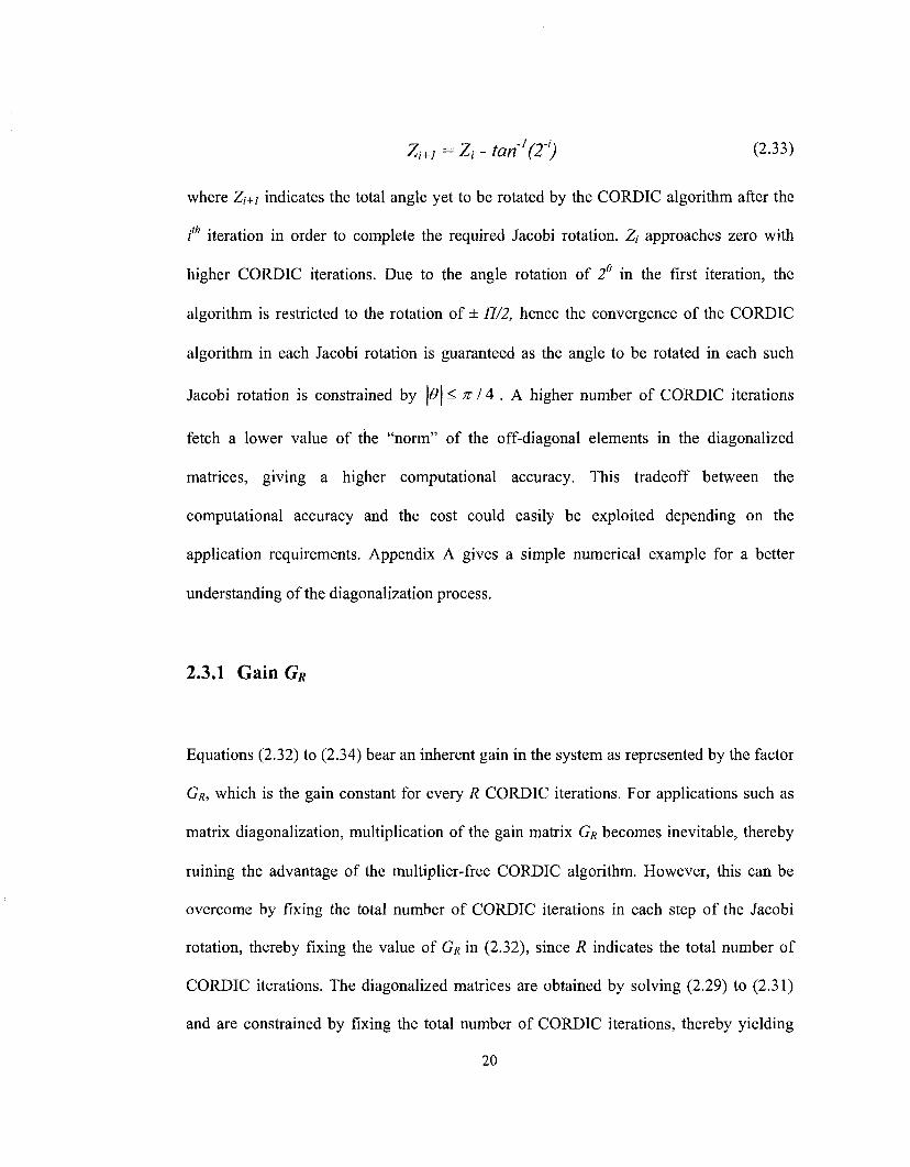
Zi+1 = Zt - tan'(I') (2.33)
where Z,+/ indicates the total angle yet to be rotated by the CORDIC algorithm after the
i'h iteration in order to complete the required Jacobi rotation. Z, approaches zero with
higher CORDIC iterations. Due to the angle rotation of 2° in the first iteration, the
algorithm is restricted to the rotation of ± 77/2, hence the convergence of the CORDIC
algorithm in each Jacobi rotation is guaranteed as the angle to be rotated in each such
Jacobi rotation is constrained by \&\< n 14 . A higher number of CORDIC iterations
fetch a lower value of the "norm" of the off-diagonal elements in the diagonalized
matrices, giving a higher computational accuracy. This tradeoff between the
computational accuracy and the cost could easily be exploited depending on the
application requirements. Appendix A gives a simple numerical example for a better
understanding of the diagonalization process.
2.3.1 GainG/j
Equations (2.32) to (2.34) bear an inherent gain in the system as represented by the factor
GR, which is the gain constant for every 7? CORDIC iterations. For applications such as
matrix diagonalization, multiplication of the gain matrix GR becomes inevitable, thereby
ruining the advantage of the multiplier-free CORDIC algorithm. However, this can be
overcome by fixing the total number of CORDIC iterations in each step of the Jacobi
rotation, thereby fixing the value of GR in (2.32), since 7? indicates the total number of
CORDIC iterations. The diagonalized matrices are obtained by solving (2.29) to (2.31)
and are constrained by fixing the total number of CORDIC iterations, thereby yielding
20

scaled diagonalized matrices. With known scaling values, the scaling could be nullified in
subsequent stages of signal processing, wherein the scaling operation can be performed
with in the filter itself without any extra hardware overhead. Therefore, the gain GR can
be neglected during the process of diagonalization of the matrices using the CORDIC
algorithm. The neglected gain is easily compensated at a later stage in the system.
2.3.2 Summary of the Algorithm
The algorithm described in Section 2.3 is summarized below. The construct 'Seq'
represents segments to be executed in sequence while the construct 'par' indicates the
segments to be executed in parallel. These are constructs similar to the ones used in a
parallel programming language like 'Handel-C to describe sequential and parallel
operations. The algorithm extracts the inherent parallel property of the CORDIC
algorithm. However, it could also be executed completely sequentially. In Chapter 4 we
implement a semi-parallel sequential architecture of the algorithm on hardware.
Algorithm: For J - 1 : Total number ofJacobi Iterations
For p = I: n-1 Par: {
For all q = {p+1 : 1: nj Seq: {
For R = 1 : Total number of CORDIC rotations Compute equations (2.29) to (2.31)
End ; Seq End
End ; Par End
End End
21

2.4 Error Analysis of the CORDIC Based Diagonalization
Engine
This section gives a graphical understanding of the computational error of the CORDIC
based matrix diagonalization algorithm. The dominating errors that affect the system
performance in a major way are the off-diagonal elements of the diagonalized matrix and
the reconstruction error from the eigen-vectors and eigen-values. It is observed through
computer simulations that the reconstruction error is predominantly due to the off-
diagonal elements, when we consider the overall system performance of a speech
enhancement system in terms of the signal to noise ratio. Detail description of the speech
enhancement system is given later in Chapter 3.
2.4.1 Mean Off Diagonal Error of the Diagonalized Matrix
Figure 2.1 shows the mean off-diagonal error of the diagonalized matrices for varying
matrix sizes, for 100 pairs of randomly generated symmetric matrices. Figure 2.1 (a)
shows the mean off-diagonal error of the matrix pairs for varying number of CORDIC
rotations, keeping the total number of Jacobi iterations to 40. Figure 2.1 (b) shows the
mean off-diagonal error of the matrix pairs for varying number of Jacobi iterations,
keeping the total number of CORDIC rotations to 30. P-Crd-x indicates the proposed
algorithm for x number of total CORDIC rotations and P-Itr-j indicates the proposed
algorithm for y number of total Jacobi iterations. A higher number of Jacobi iterations
22
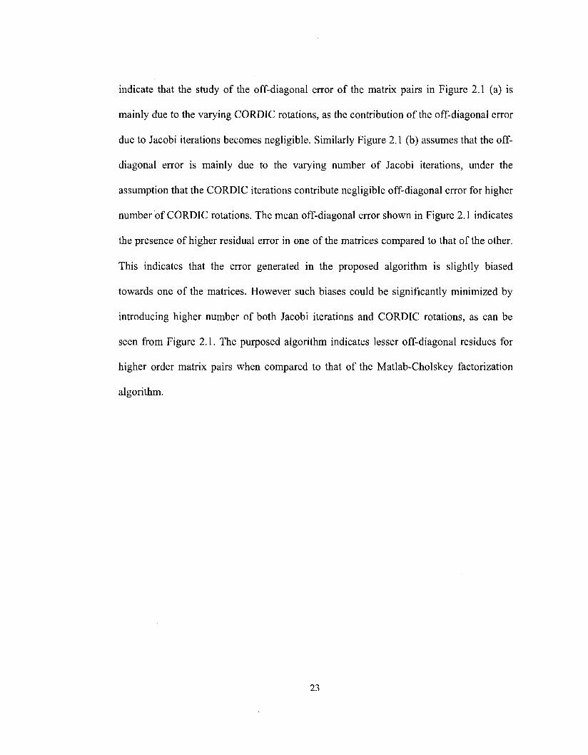
indicate that the study of the off-diagonal error of the matrix pairs in Figure 2.1 (a) is
mainly due to the varying CORDIC rotations, as the contribution of the off-diagonal error
due to Jacobi iterations becomes negligible. Similarly Figure 2.1 (b) assumes that the off-
diagonal error is mainly due to the varying number of Jacobi iterations, under the
assumption that the CORDIC iterations contribute negligible off-diagonal error for higher
number of CORDIC rotations. The mean off-diagonal error shown in Figure 2.1 indicates
the presence of higher residual error in one of the matrices compared to that of the other.
This indicates that the error generated in the proposed algorithm is slightly biased
towards one of the matrices. However such biases could be significantly minimized by
introducing higher number of both Jacobi iterations and CORDIC rotations, as can be
seen from Figure 2.1. The purposed algorithm indicates lesser off-diagonal residues for
higher order matrix pairs when compared to that of the Matlab-Cholskey factorization
algorithm.
23
5
0.2
0.18
0.16
0.14
0.12
0.1
0.08
0.06
0.04
0.02
0
-X - -£f- r
-4fc^.
-e — P-Crd-5 -A — P-Crd-10 - i P-Crd-20 -*• — P-Crd-30 * — Matlab
-TS^-7 - + o
! 15
n 6
0.35
0.3
0.25
0.2
0.15
0.1
0.05
— P-Crd-5 — P-Crd-10 — P-Crd-20 — P-Crd-30 — Matlab
20 40 60 Matrix size NxN
80 20 40 60 Matrix size NxN
80
(a)
6
0.25
0.2
0.15
0.1
0.05
1 i \ i
1 1
— e - p-itr-5 — A P-ltr-10
1 P-ltr-20 — + _ p.|tr-40
* Matlab
; \ ; _L 1 i>
> l l i l l
i l l l 1 l
1 1 1
0.35
CM X
0.25
5
0 20 40 60 Matrix size NxN
80
0.15
0.05
20 40 60 Matrix size NxN
(b)
Figure 2.1. Mean Off diagonal error of the diagonalized matrix for varying matrix sizes,
for 100 pairs of randomly generated symmetric matrices, (a) for varying CORDIC
rotations and (b) for varying Jacobi iterations.
24

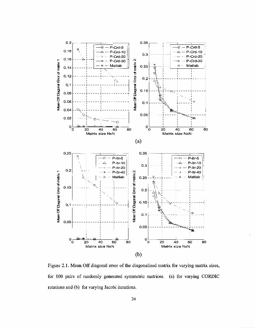
2.4.2 Mean Reconstruction Error of the Constructed Matrices
Figure 2.2 shows the mean reconstruction error of the matrices constructed from the
calculated eigenvectors and eigenvalues for varying matrix sizes, for 100 pairs of
randomly generated symmetric matrices. Figures 2.2 (a) shows the mean reconstruction
error for the matrix pairs for varying number of CORDIC rotations, keeping the number
of Jacobi iterations to 40. P-Crd-x indicates the proposed algorithm for x number of total
CORDIC rotations and P-Itr-y indicates the proposed algorithm for y number of total
Jacobi iterations. Figure 2.2 (b) shows the mean reconstruction error for varying total
number of Jacobi iterations, keeping the number of CORDIC rotations to 30. The mean
reconstruction error shown in Figure 2.2 indicates that the proposed technique clearly out
performs the Matlab-Cholesky factorization. This is as expected since the eigen vectors
generated by the proposed method are highly orthogonal and their orthogonality is well
preserved in each CORDIC rotation and Jacobi iteration. Section 2.3 explains this in
more detail.
25
1.8
1.6
1.4
1.2
1
0.8
0.6
0.4
0.2
0
1.4
1.2
0.8
0.6
0.4
0.2
— e — P-Crd-5 — A — P-Crd-10
1 P-Crd-20 * — P-Crd-30 ik - Matlab
CM
1.4
1.2
0.8
0 .6
0.4
0.2
20 40 60 Matrix size NxN
80
(a)
-\-l ^K
— P-ltr-5 — P-ltr-10 — P-ltr-20 — P-ltr-40 — Matlab
CM
x
0.9
0.8
0.7
| 0.6
"ft
$ 0.4
20 40 60 Matrix size NxN
80
0.3
0.2
0.1
0
20 40 60 Matrix size NxN
1 I
TV" i i -
— e — P-ltr-5 —<£> — P-ltr-10 -
1 P-ltr-20 *- — P-ltr-40 -
— * — Matlab
\ \ i * '
.... Kb,. 1 1
^
20 40 60 Matrix size NxN
80
(b)
Figure 2.2. Mean reconstruction error of the constructed matrices from the calculated
eigen-vectors and eigen-values for varying matrix sizes, for 100 pairs of randomly
generated symmetric matrices, (a) for varying CORDIC rotations and (b) is for varying
Jacobi iteration
26
2.5 Summary
In this chapter we have presented a brief introduction to the Jacobi based matrix
diagonalization technique for symmetric matrices. This well known technique is a
computationally efficient numerical technique for symmetric matrix diagonalization
problems. This technique also provides an intuitive mechanism for parallel
implementation. However, in practice, a complete parallel implementation becomes
unreasonable for very large matrix sizes due to an exponential increase in the hardware
requirements; hence, mostly a folded semi-parallel approach is very often preferred.
This chapter has also reviewed the basics of the CORDIC algorithm. The
CORDIC implementation exploits the advantage of mapping powers of 2 constant
coefficient multiplications effortlessly onto digital hardware, thereby reducing the
computational elements to a set of shift and addition operations. At the core of the
CORDIC algorithm is the iterative vector rotation, which has a very high convergence
rate.
We have further presented a simple extension of the Jacobi algorithm for
simultaneous diagonalization of multiple symmetric matrices, which has been efficiently
mapped onto the CORDIC implementation scheme, thereby making a complete
multiplier-free implementation of the simultaneous diagonalization technique possible.
Being iterative in nature, for most practical applications, it provides an easy tradeoff
between the computational accuracy and the execution speed. The error analysis of the
proposed technique shows a performance similar to that of the Matlab-Cholesky
factorization as the size of the matrices increase.
27

Chapter 3 : Speech Enhancement
Speech enhancement is the term used to describe the process of improving the perceptual
aspects of human speech. With the increase of digital communication in the last 50 years,
speech enhancement has attracted increasing attention in different speech processing
problems. Speech enhancement primarily consists of removal of noise from degraded
speech while maintaining the speech quality over an audible threshold.
3.1. Review of Subspace Based Speech Enhancement
Technique
The application of signal subspace approach has traditionally found its place in frequency
estimation, direction of arrival estimation and system identification [64], [59], [39]. It is
only recently that it has been applied for speech enhancement applications. The basic
concept is to project the noisy speech signal onto two subspaces: the signal-plus-noise
subspace and the noise subspace. As the noise subspace contains only the noise process,
the signal can be recovered by removing the components of the signal in the noise
subspace while retaining the components of the signal in the signal subspace. The
decomposition of the signal into its subspaces is usually done by either using the singular
28
value decomposition (SVD) [63], [59] or the eigen value decomposition (EVD) [56],
[10], [64], [39] .
Dendrinos et al. [63] have proposed a SVD-based technique making use of the basic
idea that the eigenvectors corresponding to the largest singular values contain signal
information, while the eigenvectors corresponding to the smallest singular values contain
noise information. Thus, the largest singular values are sufficiently informative enough to
reconstruct the enhanced signal. This has given impressive SNR improvements mostly
for signals corrupted with white noise. The work of Dendrinos et al. [63] was further
extended by Jensen et al. [59] using the Quotient SVD (QSVD) approach to tackle the
problem of removal of colored noise. By arranging the signal data in a Toeplitz matrix,
they arrange the data in a Hankel matrix and compute the least square estimate of the
signal-only Hankel matrix. However, the computational inefficiency of the QSVD, along
with its inability to either shape or control residual noise, is not attractive. Ephraim and
Van Trees [19] then came up with an optimal estimator that would constrain the residual noise
while minimizing the speech distortion. This essentially leads to solving a constrained
minimization problem. This technique uses the Karhunen-Loeve transform (KLT), which
decomposes the vector space of the noisy signal into a signal and noise subspace. The
estimated signal is then obtained by performing an inverse KLT after nullifying the noise
components from the signal and noise subspaces in the KLT domain. The traditional
spectral subtraction method that introduces a lot of musical noise is overcome by the sub-
space approach, yielding a much better speech quality. Ephraim and Van Trees's
formulation of the subspace approach is based on the assumption that the input noise is
white. Their work was further enriched by Yi, Hu and Loizou by their generalized
subspace approach for enhancing speech that is corrupted by colored noise [19]. This lead
29
to an optimal linear estimator that minimizes the speech distortion while suppressing the
background noise, using time-domain constrains (TDC). The following sections highlight
the theory behind the design of a subspace approach speech enhancement engine based
on certain time domain constraints for handling colored noise.
3.1.1 Optimal Subspace Filter for Speech Enhancement
A linear speech production model is assumed for clean speech X, given by, X = ¥ S,
where ¥ is a K x M matrix with rank M (M < K) and 5 is a M x 1 vector, respectively.
The covariance matrix of X, which is also a positive definite matrix, is given by
Rx = E{X XT) = W RXWT (3-1)
Since the rank of the matrix Rx is M, it has K - M zero eigen-values. With the
assumption that the noise is additive and uncorrelated with the speech signal, the
corrupted signal is given as
Y=W S + d = X+d (3.2)
where Y, X and d are the ^-dimensional noisy speech, clean speech and noise vectors
respectively. The linear estimator X of the clean speech X is given by, X = H.Y, where
H is a K x K matrix. This estimate would essentially generate an error signal e due to the
incorrect estimate of the signal and is given by
E=X-X=(H- I)X + H d= Ex+ed (33)
30

where e represents the speech distortion and e, the residual noise [19]. The associated X
energies s?x and sd of the distortion signal and the residual noise are given by
4 = E[eTx ex] = tr(E[eT
x e J ) = tr (HRX HT - HRX - RXHT + Rx)
and 7d = E[eTded] = tr(E[eT
ded]) = tr (HRdHT) (3.4)
The optimal linear estimator is obtained by solving the linear time-domain constrains,
leading to the solution of a constrained minimization problem. Essentially, the estimator
estimates the enhanced speech keeping the speech distortion below a threshold, which is
adaptively set for every speech frame. The constrained minimization problem is given
below.
Minimize : sx
Subject to: -£2d^
d ( 3 5 )
where a is a positive constant. The solution to the above constrained equation is given
by [19]
Hopt=Rx(Rx+M.Rdy> <3-6)
where Rx and Rd are the covariance matrices of the clean speech and noise, respectively,
and ju is the Lagrange multiplier. After using the eigen-decomposition of
RX—UAXU , the simplified estimator is given by
Hopt= U\(AX+ fiUTRdUf' If (3.7)
31

where U and Ax are, respectively, the unitary eigenvector matrix and the diagonal
eigenvalue matrix of Rx. In the case of white noise with variance 0d , Rd = Od I and the
estimator described above reduces to that of Ephraim and Van Trees [19]. It basically
approximates /^by the diagonal matrix
&d=diag(E(\u]d\2), E(\uT2d\2), ..., E(\uT
Kd\2)) ( 3 8 )
where £4 and d are, respectively, the K: eigenvector of Rx and the noise vector
estimated from the speech-absent segments of speech. Thus, the approximated sup-
optimal estimator developed by Ephraim and Van Trees, which is not suited for colored
noise is given by
Hopt*UAx(Ax+MAdyluT ( 3 - 9 )
Later the work was improved by Hu and Loizou [19], by studying the matrix U Rd
U, which they found to be weakly diagonalizable. This is not surprising, since the
eigenvectors of Rx, which are supposed to diagonalize Rd could diagonalize Rd only in
the case of white noise. On the contrary, it can be shown [28] that there may exist an
eigen-space, which is common to both the matrix spaces Rx and Rd, thus essentially
resulting in the simultaneous diagonalization of both Rx and Rd- The simultaneous
diagonalization as given by [19] is as follows:
VTRXV = A£
VTRdV=I (3.10)
32
where Aj; and V are the eigen-value and eigen-vector matrices respectively. Using the
eigen-decomposition of Rx and Rj, the optimal estimator is further simplified as shown
below.
Hopt=RdVAsUE+liI)-1VT
= V-TA£(AZ+MI)-1VT (3.11)
It has been shown in [19] that the Lagrange parameter ju must satisfy
S2={tr{(VTrfAl(A£+Miy2} ( 3 1 2 )
where sd = Kd . The enhanced signal is obtained by X = Hopt Y, where Y is the noisy
input speech signal. This fundamentally amounts to a transform V being applied to the
noisy signal Y and then the enhanced signal X estimated by appropriately applying a gain
function in the transformed domain and then taking the inverse transform (V ) of the
modified components, as shown by (3.11). The gain matrix is given by
G = A% {Ax + pt I)' , a diagonal matrix.
3.1.2 Estimating the Lagrange Parameter fi
So far we have described the optimal estimator as given by (3.11); however, it requires
the calculation of the Lagrange parameter ju. Ideally, to parametrically compute the
Lagrange parameter pi, it would require solving (3.12), which is certainly not a trivial
task. Therefore, an approximation of the Lagrange parameter is the next option.
33
Estimation of // involves the risk of either over estimating the parameter resulting in a
high back ground noise suppression but with heavy speech distortion, or an under
estimation of the parameter that would lead to minimum speech distortion but low back
ground noise suppression. Hence, the estimate of the parameter // is critical.
Ideally, we would like to minimize the speech distortion in speech-dominated frames,
since the speech signals will have a masking effect on the noise; hence, the value of //
would then be dependent mostly on the short-time SNR. Hu and Loizou [19], therefore,
chose the following equation for estimating pi:
M = Mo-(SNRdb)/s (3.13)
where pio and s are constants chosen experimentally, and SNR^b = lOlogio SNR. It is to
be noted that a similar equation was used in [19] to estimate the over-subtraction factor in
spectral subtraction. However, it has been shown that the method proposed by Hu and
Loizou provides a better trade-off between speech distortion and residual noise compared
to the approach in [19], which uses a fixed value of pi regardless of the segmental SNR.
The estimate of the SNR is found directly by replacing the signal energy by their
m eigen-values, X E along with their corresponding eigenvectors V/c
[i.e., Xf=E{\v{x\2)),
tr(V%V) Zf^f (3.14) SNR = T
tr (Rx) The segmental SNR definition thus reduces to the traditional SNR definition of—-—-tr {Rd)
for an orthogonal matrix V.
34

3.2. Frequency Sub-Band Processing into Subspace based
Speech Enhancement
In this section, we develop a technique to tackle the problem of inaccurate estimation of
the covariance matrices, keeping in mind the masking properties and computation
complexities. We address this by focusing on the subbands rather than treating the full
band signal. The subband approach exploits the inherent low variance of the speech and
noise signals in a limited frequency region as opposed to using the full band. This
technique automatically results in subband-based covariance matrices that are much more
accurate compared to the full band counterpart. This accurate estimate of the covariance
gives a better estimate of the clean speech under heavy noise conditions, as will be
evidenced by the results obtained (see Section 3.3.5.). Further, by using the frequency
sub-band technique we can update the covariance of the noise and noisy speech
independently in each subband. This is possible since many of the frequency subbands do
not often contain speech activity, even though there is activity in the other subbands. Thus,
even though there may be speech detected in the full-band signal, the subband technique
offers a better covariance estimation by allowing band selective covariance update in
contrast to the full band approach. The subband technique involves simultaneous
diagonalization of much smaller matrices compared to the full band case. This not only
results in a higher accuracy, as will be seen from computer simulations, but also reduces
the computational cost, since the computational complexity for matrix diagonalization
increases as the cube of the size of the matrix [73].
35

3.2.1. Theory of Frequency Sub-Band Processing
The subband implementation of the subspace enhancement scheme is illustrated by the
block diagram in Figure 3.1. As a first step, the noisy speech signal is broken down into
M narrow band frequency segments using a perfectly re-constructible filter bank
followed by down sampling, as shown in Figure 3.1. Letyj, Xj and rij denote the noisy
speech, clean speech and noise signals in t h e / frequency sub-band. Then, assuming an
additive noise model we obtain
y=Xj+nj
where the noise and speech are assumed to be uncorrelated in each subband.
(3.15)
Input
Signal
("N' points/ frame)
Ix tx
F i 1 t e r
B a n k
tx
Down sampling
by'M'
m M
Subband Speech/Pause
Detection
Subband SHR Estimator
4M
'M' Subband
Decomposition Filter Bank
Subband Filter
Estimator
Up sampling
by'M'
fM
-» Subband Speech/Pause
Detection
Subband SNR Estimator
P
* Subband Filter
Estimator
+ -HtM
tx tx
F i 1 t e r B a n k
tx
Output
Signal
— • ("N1 points/
frame)
Subband Filtering with WM' Samples per frame
M' Subband Reconstruction
Filter Bank
Figure 3.1 System Overview
36
Now, in each subband, an independent subspace speech enhancement linear estimator is
employed to obtain the enhanced speech in that particular subband. Let Hj be the optimal
linear estimator for they'"' subband; then, the clean speech estimate Xj in that subband is
obtained by Xj = Hj. Yj , where Hj is a KxK matrix. The error signal is given by
SJ =XJ +XJ = (Hj-I)xj + Hj T V S ( 3 , 1 6 )
where the two error components e .̂and en. denote the speech distortion and residual
noise for the / subband. The corresponding energy components could be expressed as
4 =E [Snj S ] = tV {E [4 Si) (3AV
Following the procedure used in [19], an optimal linear estimator can be derived by
considering the following constrained optimization problem, where the speech distortion
term in (3.17) is minimized subject to the constraint that the residual noise error term in
(3.18) is reduced to a value that is lower than the threshold:
Minimize: si. Xj
Subject to: - e2n. < d) (319)
where, 8. is a positive constant in each subband and is assumed to be a function of the
subband segmental signal to noise ratio (SSNR) in our case. The constrained
minimization in (3.19) leads to an optimal filter
37

Hj= RXj(RXj+HjRn) (3.20)
where pi. is the Lagrange multiplier, and Rx, and Rn. are the KxK clean speech and noise
covariance matrices, respectively. In each segmental frequency, a decision is made to
distinguish between a pause frame and a speech frame based on a simple comparison of
the present frame energy to that in the past few frames. Based on this decision, an update
of the autocorrelation of the noise or speech is estimated, using which the linear estimator
is constructed. As shown in [19], the simultaneous diagonalization of Rx. and Rn.
generalizes the optimal estimator in (3.20) to handle the case of colored noise when
VfRnjVj = I (3.21)
where Ax. and V.- are the subband eigen vectors and eigen value matrices, respectively.
Applying the eigen decomposition of (3.21) in (3.20), we can rewrite the subband linear
estimator as
H.=R (R +u.R Y=VrTA ( A +u.lYvT=V.G.VT n22) j XJ \ XJ r*j nj J j xj\ xj r~j ) j j J J l J - z z y
where the gain matrix Gj is a diagonal matrix that is intended to attenuate the eigen
values of the autocorrelation of the noise according to the Lagrange parameter fij. As
mentioned earlier, this parameter is very important. It determines the amount of speech
distortion for a minimum noise residue in the corresponding subband. A large estimate of
this parameter would eliminate much of the background noise at the expense of
introducing speech distortion and conversely, a small estimate would minimize the
speech distortion at the expense of introducing large residual noise. It has been shown in
38

[19] that//,- does not have a closed form expression in terms of 8 , which forces the use
of a linear expression for the Lagrange parameter, as done in [19]. The Lagrange
parameter thus obtained is then scaled by the SSNR of they' subband. This incorporates
the subband Lagrange parameter as a function of the SSNR in that frequency band. The
estimated signal from each frequency segment is up sampled and reconstructed in the
filter bank to generate the final full band estimated signal.
3.2.2. Justifying the Need for Sub-Band Processing
The proposed subband technique assumes that the noise is uncorrelated in each of the
subbands and may or may not be uncorrelated in the over-all signal. Thus, the approach
proposed here is a more generalized one. Computer simulations indicate that the
simultaneous diagonalization of Rx. and Rn. in each subband has a greater degree of
accuracy in terms of numerical computations as compared to that in the full band
approach. The down sampling in the filter bank drastically reduces the matrix size in each
subband as compared to that in the full band case. This reduces the computation
complexity of the diagonalization unit, since the computational complexity increases as
cube of the order of the matrix. Speech frames are taken at a speech length of 32 ms in
order to preserve speech property, from which enhancement is possible [67]. A 32ms of
speech on an 8000 sample/s sampling rate would require a buffer length of 256 words,
with a simultaneous diagonalization core of the order 256. On the contrary, with a 4
channel filter bank, it would require 4 individual buffers of length 64, with the
simultaneous diagonalization core to only handle matrices of order 64. As the cube of 64
39

is a much smaller number than that of 256, the increase in hardware due to the 4 channel
filter bank is well compensated by the reduced hardware in the matrix diagonalization
engine. It will be shown in Chapter 4 that the hardware complexities of higher order
diagonalization engines result in lower throughput, which is the primary bottle neck in
processing higher signal rates. Hence, the frequency subband technique also provides a
solution for parallel implementation of speech enhancement in dealing with signals of
higher sampling rates.
3.3. Objective Performance Measures and Experimental
Results
In this section, we will fist describe the objective measures that have been used for
quantitative performance measure of the overall system performance. We will then
present the experimental results of the sub-band based speech enhancement engine.
3.3.1. Signal to Noise Ratio (SNR)
SNR is the most often chosen measure because of its computation simplicity. Let y(n),
x(n) and d(n) denote the noisy speech signal, clean speech signal and noise signal,
respectively, and x(n) the corresponding enhanced signal. The error signal e(n) can be
written as
40

e(n) = x(ri) - x\n)
The error signal energy can be computed as
n n
and the signal energy as
Ex= I,nx2(n)
The resulting SNR measure (in db) is obtained as [69], [68]
(3.23)
(3.24)
(3.25)
SNR = 10logJ0^h=10log Zn*\n) '10 In [*(«)" *(»)]'
(3.26)
3.3.2. Segmental SNR (SSNR):
The SSNR measure is a variant of the SNR, and is formulated as follows [68], [69]
SNRseg=^llOlog10 n = mi- N + 1
i:j N+Mri)-mv
n=m: - N + 1 (3.27)
where mo, mi, ... , mu-i are the end-times for the M frames, each of which is of length
N. For each frame, the SNR is computed and the final measure is obtained by averaging
these measures over all the segments of the waveform. For some of the frames, the SSNR
is either unrealistically high or unrealistically low, thus providing a biased estimate of the
SSNR. This issue is addressed by discarding the SSNR values below or above a
predefined lower or upper SSNR threshold value, respectively. In this work, we have set
the higher threshold value to be 35 db and the lower one to be -10 db.
41

3.3.3. The Itakura Saito distance (ISD) Measure:
The ISD measure is based on the linear prediction (LP) coefficients. Specially, for each
frame m, we obtain the LP coefficients a(m) of the clean signal and the LP coefficients
P(fri) of the enhanced signal. The ISD measure is defined by [68], [69]
[q(m) - p(m)] TRx{m)[a(m)-P(m)\
d{m) j a(m) Rx(m)a(m) (3.28)
where Rx(jn) is the autocorrelation matrix of the mth frame of the clean speech.
3.3.4. Modified Bark Spectral Distortion (MBSD) Measure:
The difference between the MBSD measure [40] and SNR, SSNR and ISD measures is
that the MBSD measure takes into account a psycho-acoustical model, which is absent in
the other three models. The MBSD measure is defined as the average difference of the
estimated loudness which is perceptible, while the bark spectral distortion (BSD) measure
is defined as the average squared Euclidean distance of the estimated loudness. The BSD
and the MBSD measures are defined by the following equations [40]:
BSD = •jj/Lj = 0 E/=7 [Lx (0 - L- (Q] ^29)
M-l
MBSD = — > I V 1
M j-o
K
^/(/)|LP(0-Lf(0 (3.30)
U = l
where./' is the frame index, Mis the number of frames, / is the critical band index, K is the
number of the critical bands, /(/) is the indicator of perceptible distortion at the /th critical
42

band, L)/\i) is the z'th band Bark-spectrum of the/h frame of the clean signal, and L~ (f)
is the ith band Bark-spectrum of the fh frame of the enhanced signal. The perceptible
indicator I(i) is set to either 1 or 0. If the difference between the bark spectrum of the
clean speech and the enhanced speech is below the noise masking threshold, indicating
that the distortion is not perceptible, the parameter I(i) is set to 0, otherwise it is set to 1
[40]. The Bark scale is a psycho-acoustical scale named in memory of the scientist
Heinrich Barkhausen (1881 - 1856), who introduced a measure for the level of loudness
[41]. The resolution of human auditory system is described by the critical band tuning
curves of the inner ear. Based on psycho-acoustical experiments [41], the frequency
range is divided into critical bands. The concept of critical bands leads to a nonlinear
warped frequency scale called the Bark scale. The unit of this frequency scale is Bark,
where each critical band has a bandwidth of 1 Bark. The transform of the frequency /
into Bark scale is approximately given by [41],
Bark = 13 arctan (0.00076 f) + 3.5arctan(( f/7500)2) (3.31)
The scale ranges from 1 to 24 and corresponds to the first 24 critical bands of hearing.
The subsequent band edges are (in Hz) 20, 100, 200, 300, 400, 510, 630, 770, 920, 1080,
1270, 1480, 1720, 2000, 2320, 2700, 3150, 3700, 4400, 5300, 6400, 7700, 9500, 12000,
15500. In this thesis, with 8000 samples/s the number of critical bands K is chosen as 18.
This also helps in an appropriate comparison of the results with those in [19].
Calculations of the/h frame Bark-spectrum has been well described in [70], where the
spectral average of the individual critical bands over the entire spectrum provides the
bark spectrum of that particular frame.
43

3.3.5. Experimental Results and Discussion
We evaluate our frequency sub-band (FS) algorithm on 20 sentences from the TIMIT
database that includes 10 male and 10 female speakers. The proposed enhancement
parameters are: sampling rate = 8 KHz, number of subbands = 32 and window size = 32.
A perfect reconstruction filter bank obtained using the 'Daubechies 18' wavelet packet
analysis function is employed. The enhanced vectors are hamming windowed and
combined using the overlap-add-synthesis method while a rectangular window is used to
estimate the covariance matrices. The clean speech files are corrupted by employing an
additive noise model, where the car, babble and F-16 cockpit noises from the NOISEX
database are added to the clean speech files at -10, -5, 0, 5 and 10 dB SNRs. Figure 3.2
shows the spectrogram of a typical clean speech of a TIMIT sequence, and Figure 3.3
those of the speech corrupted by the car noise at -10 db SNR and the corresponding
speech after the proposed filtering. The FS algorithm is compared against Ephraim-Van
Trees (EV) [19] and Hu-Loizou (HL) [19] subspace schemes, using three evaluation
measures, namely, the segmental SNR, the Itakura distance and the MBSD. A
comparative analysis of the three algorithms in terms of the above mentioned objective
measures are illustrated in Figures 3.4, 3.5 and 3.6 for the car, babble and F-16 cockpit
noises. It is easily seen that the proposed FS technique outperforms the EV and HU
methods from the point of view of all the three measures under low SNR conditions. The
improvements are substantial at very low SNRs of -10 and -5 dB and diminish with
increasing SNR, as is to be expected.
44
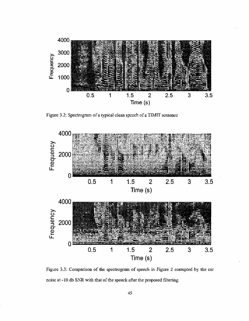
Figure 3.2: Spectrogram of a typical clean speech of a TIMIT sentence
4000
o
§ 2000 a-
CD !s*- 1*-
0.5 1.5 2 Time (s)
4000
o
I 2000 cr
0.5 1 1.5 2 2.5 3 3.5 Time (s)
Figure 3.3: Comparison of the spectrogram of speech in Figure 2 corrupted by the car
noise at -10 db SNR with that of the speech after the proposed filtering.
45
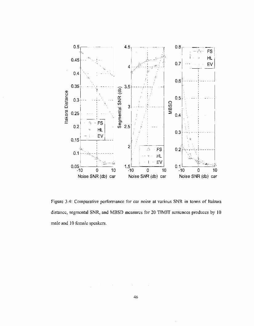
0.5
0.45
0.4
0.35 CD O
I 0.3
1 0.25 CD
-t—»
0.2
0.15
0.1 0.05
k I "4
\ ' ^\ T- -J- - - ^ - |
X '
\k
\
;.....
- A FS
* HL EV
---;-
V ! /'-V^ i
4.5
3.5
or z CO
•4—'
c CD
E CD
to 2.5
1.5
FS HL EV
a C/) CO
u.u
0.7
0.6
0.5
A FS
* HL EV
~ r •
0.4
0.3
0.2
- • - - - -
..._ >._ T. _ —
V u \
-10 0 10 -10 0 10 Noise SNR (db) car Noise SNR (db) car
0.1 -10
\ V v
0 10 Noise SNR (db) car
Figure 3.4: Comparative performance for car noise at various SNR in terms of Itakura
distance, segmental SNR, and MBSD measures for 20 TIMIT sentences produces by 10
male and 10 female speakers.
46

CD O
c
2 w b CD i _ O ^. CO
0.35
0.3
0.25
0.2
0.15
0.1/
0.05
0
+
"A-
FS
HL
EV
4.5
| 3.5 </)
I * CD
2.5
1.5
—A— FS
=< HL
_ + _ EV
'"""1? / ' *
/ ; , I { -'~ - - ;' -i - - •• -
/ / '
--i
X—
1
0.5
0.45-
0.4
0.35
| 0.3
0.25
i
0.2
0.15
0.1
:
\
- - -J
I
- V-. -
•
-
_
• • -
--
s -
&;
\
_A-
*
1 -
I ._
r ~i
i ~
i _
", " t ~~
Jk
- F S
HL - E V
V-3 -10 0 10 -10 0 10 -10 0 10
Noise SNR (db) babble Noise SNR (db) babble Noise SNR (db) babble
Figure 3.5: Comparative performance for babble noise at various SNR in terms of Itakora
distanc, segmental SNR, and MBSD measure for 20 TIMIT sentences produces by 10
male and 10 female speakers.
47
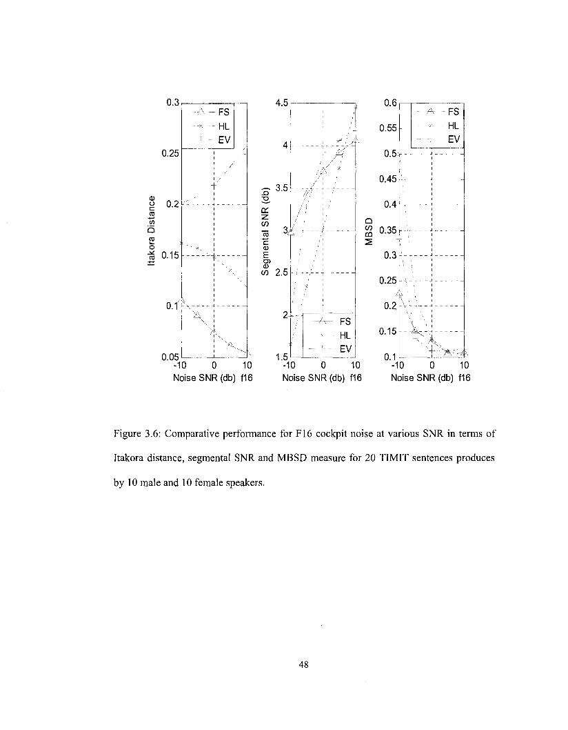
O c
Q
o
0.3
0.25
0.2
0.15
0.1'
0.05
/- FS
- HL
EV
-_
_'v 1
1 v£^»
4.5
- 3 . 5
01 z - 3 B CD
E CD
w 2.5
0.6
0.55
0.5
0.45
0.4
| 0.35
0.3
0.25
-10 0 10 Noise SNR (db) f16
-10 0 10 Noise SNR (db) f16
0.2
0.15
0.1
---
r ~
(Z) —
1 >
U.
I H
I
J
-- - -1 - -
V x I
1 ^& -10 0 10 Noise SNR (db) f16
Figure 3.6: Comparative performance for F16 cockpit noise at various SNR in terms of
Itakora distance, segmental SNR and MBSD measure for 20 TIMIT sentences produces
by 10 male and 10 female speakers.
48

3.4. Summary
In the initial section, the basics of a subspace based speech enhancement system have
been reviewed. In the subsequent sections an innovative subband-based speech
enhancement analysis technique that exploits the slow varying characteristics of speech
and noise signals over narrow frequency segments, has been proposed. The accurate
covariance estimation of the noise and speech in the subband results in a better
performance in low SNR conditions as compared to that of full band subspace-based
speech enhancement techniques. The proposed technique also provides for an inherent
parallel implementation scheme and reduces the computational complexity. The proposed
scheme makes no assumptions of the spectral characteristics of the noise, but only assumes
that the noise and speech are uncorrelated in each of the subbands. The performance of the
proposed scheme has been evaluated in terms of the Itakora distance measure, segmental
SNR and modified bark spectral distortion measure (MBSD), and compared with that of two
of the well-known full band subspace-based speech enhancement techniques, namely, the
subspace based speech enhancement developed by Ephrime and Van Trees, and the
generalized subspace based speech enhancement for coloured noise by Yi Hu and Loizou.
Improvement in speech enhancement using the subband-based subspace speech enhancement
technique is clearly visible from the results that have been obtained.
Having presented the subband-based subspace speech enhancement algorithm in this
chapter, the next chapter, Chapter 4 presents an hardware architecture for implementing
the speech enhancement algorithm on FPGA. The architecture utilizes the simultaneous
diagonalization algorithm discussed in Chapter 2 and implements a subspace-based
speech enhancement processor.
49

Chapter 4 : Multiplier-Free Architecture
for the Proposed
Simultaneous Diagonalization
Scheme
So far we have described a CORDIC based algorithm for simultaneous symmetric matrix
diagonalization. We have also presented a frequency-subband speech enhancement
algorithm. In this chapter, we will describe the hardware architecture that efficiently
diagonalizes the symmetric covariant matrices of speech and noise, and computes the
optimal estimator, using which we enhance the noisy speech, thus rendering it to be a
speech enhancement processor. The necessary supporting hardware modules such as the
memory modules and controllers are also presented. The architecture is coded in VHDL
using the Xilinx ISE design flow to target a FPGA implementation. All the simulation
results are obtained using the ModelSim simulation software from Mentor graphics. The
time limitation of this Master's thesis has compelled the use of FPGA due to its shorter
design time compared to that of an ASIC counterpart. However, in Chapter 5, a
projection of an ASIC equivalent implementation is studied from the perspective of total
transistor count only.
The speech processor has been divided into the following sub-blocks.
1) Eigen domain Filter
2) Memory Architecture
50
The subsequent subsections explain the architecture in detail. However, the experimental
results of their FPGA implementation in terms of the hardware utilization and the overall
system performance measures are discussed in Chapter 5.
4.1. Architecture of the Eigen Domain Filter
The eigen-domain filter is responsible for the process of speech enhancement on a frame
by frame basis. The core of this filter is a CORDIC based diagonalization engine
(described in Chapter 2), which simultaneously diagonalizes the two symmetric covariant
matrices. Apart from the CORDIC core, the eigen-domain filter consists of other units as
well. This includes the autocorrelation unit, eigen-domain filter gain calculation unit, and
a multiply and accumulate (MAC) unit for executing matrix multiplications which make
up the entire eigen-domain filter. Dividing the design into subparts also makes
designing, testing, debugging and design-reusability easier and convenient. The following
are the sub-blocks of the eigen-domain filter:
1) CORDIC architecture of a single processing element (PE)
2) Multiply and accumulate (MAC) unit
3) The autocorrelation unit
4) Eigen domain filter gain calculation unit
5) Jacobi pair (P, Q) generation Unit
51
4.1.1. CORDIC Architecture of a Single Processing Element
The proposed architecture of a single processing element (PE) is shown in Figure 4.1.
The operation of the PE is divided into two modes: first, finding the appropriate direction
of the CORDIC rotation and second, the CORDIC transform. In the first part of the PE
operation, the desired CORDIC direction is computed, as given by (2.30) and is stored in
the 1-bit sign register, sign(0), shown in Figure 4.1. In the second mode, the CORDIC
rotations, as given by (2.29) to (2.31), are computed based on the sign which is already
computed in the previous mode. This completes one single CORDIC iteration. The
architecture is fully pipelined for maximum performance in terms of the data transfer
rates. Due to the shift and add nature of the operations given by (2.29) to (2.31), the
architecture is well suited for FPGA/ASIC implementation. At the beginning of the
diagonalization process, the eigen-vector matrix V is initialized to an identity matrix.
Since the CORDIC iteration is an orthogonal transform, the resultant eigenvector matrix
V is also an orthogonal matrix. The covariant matrices that are to be simultaneously
diagonalized are symmetric, and as a result, the eigen-values and eigen-vectors are also
real. This discards the need for complex arithmetic units. A single PE unit computes one
CORDIC iteration as given by (2.29) to (2.31), and R such rotations complete a single
Jacobi iteration. To achieve higher data rates, a number of such PE units could be
cascaded to increase the overall throughput. This also makes the architecture very
scalable. There are four registers in between the adders that act as pipeline registers. The
architecture given in Figure 4.1 has serial data I/O interfacing in order to decrease the
total number of I/O pins used by this unit. Figure 4.2 shows the I/O block diagram of the
52
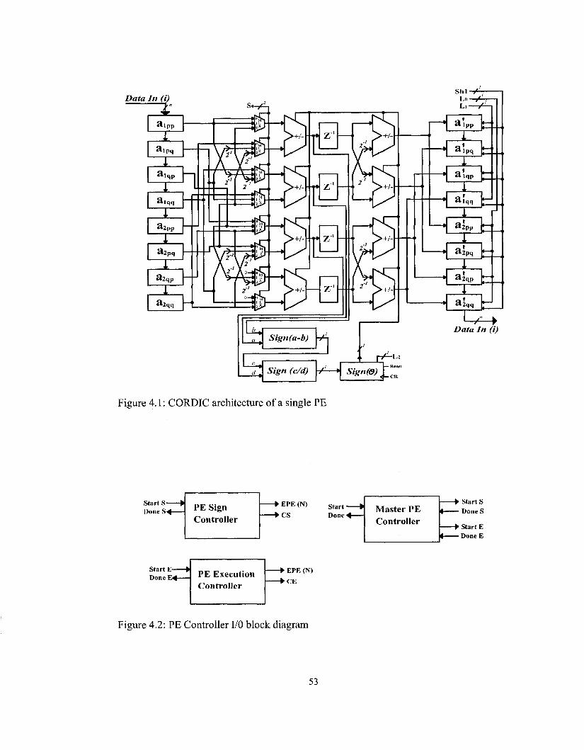
Data In (i)
a ) p q
zzt: a l q p m a qq
I a2 pp
X a2 p q
a2 q p
in a*,, K
Sign(a-b)
Sign (c/d) * »\ Sign(e)l_
L2 Reset
Clk
S h i - / - ;
L i — ^ - 1
H aw b-
H a«qq
T •H a 2 p p
E •I a2 p q ^ x
a2l qp
I aiqq t
Z)«to In (i)
Figure 4.1: CORDIC architecture of a single PE
» EPE (N)
• CS Start -Done<
Master PE Controller
— • Start S Done S
— • Start E i Done E
Start E Done PE Execution
Controller
• EPE (N)
•CE
Figure 4.2: PE Controller I/O block diagram
53
PE controller units. These controllers are basic state machines, controlling the state
transition of the PE unit. The next section describes the state transition of the controllers
in brief, through finite state machine (FSM) diagrams. The controllers are responsible for
synchronous operations within each PE. The controller unit consists of a PE master
controller which in turn synchronizes and controls the PE sign controller and the PE
execution controller. Figure 4.3 shows the timing diagram of some of the important I/O
signals of a single PE.
(a) PE Master Controller FSM Design
The PE master controller synchronizes the operation between the PE sign controller unit
and the PE execution controller. The FSM of the PE master controller is shown in Figure
4.4. It operates on two 2-by-2 matrices and calculates (2.29) to (2.31). Controlled by the
"start PE controller Unit" control signal to start the operation, the PE master controller
asserts the "Done PE Controller" at the end of the execution.
(b) PE Sign Controller
The PE sign controller is responsible for calculating the direction of the CORDIC
rotation as given by (2.33). Figure 4.5 describes the FSM of the sign controller. In the
first eight clocks, the input data vector is loaded through the data in bus on to the shift-in
registers. Subsequently the sign of the angle to be rotated is computed as given by (2.33).
Parameters such as P and N are internal counters that are used by the FSM to keep track
54
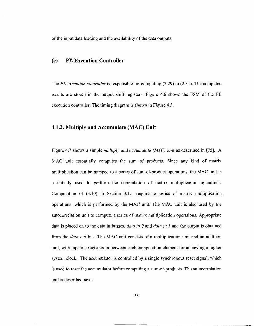
of the input data loading and the availability of the data outputs.
(c) PE Execution Controller
The PE execution controller is responsible for computing (2.29) to (2.31). The computed
results are stored in the output shift registers. Figure 4.6 shows the FSM of the PE
execution controller. The timing diagram is shown in Figure 4.3.
4.1.2. Multiply and Accumulate (MAC) Unit
Figure 4.7 shows a simple multiply and accumulate (MAC) unit as described in [75]. A
MAC unit essentially computes the sum of products. Since any kind of matrix
multiplication can be mapped to a series of sum-of-product operations, the MAC unit is
essentially used to perform the computation of matrix multiplication operations.
Computation of (3.10) in Section 3.1.1 requires a series of matrix multiplication
operations, which is performed by the MAC unit. The MAC unit is also used by the
autocorrelation unit to compute a series of matrix multiplication operations. Appropriate
data is placed on to the data in busses, data in 0 and data in 1 and the output is obtained
from the data out bus. The MAC unit consists of a multiplication unit and an addition
unit, with pipeline registers in between each computation element for achieving a higher
system clock. The accumulator is controlled by a single synchronous reset signal, which
is used to reset the accumulator before computing a sum-of-products. The autocorrelation
unit is described next.
55
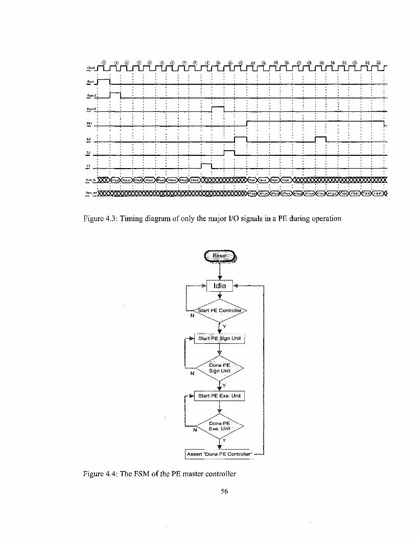
Start | | '. i
Start S
Start E
Shi
LO
LI
L2
1 j :
Data-in XXXX , 1<wX a , < ' , ' < i *XB I ( ' i ' , ,X l , l t ,M ) )^i<p'PXaI(i,'q)Xa2<,''P1i
• i—i
: : • 1
i—i i—i
'a2<<i,q> XXXXXXXXXXXXXX^** ] (y(pA) X(i-|>tJ
1
•
(V<M> XXXXXXXXXXXXXXXXXXXXXXXXXXX
Figure 4.3: Timing diagram of only the major I/O signals in a PE during operation
C Reset J 4
Idle
Assert "Done PE Controller"
Figure 4.4: The FSM of the PE master controller
56
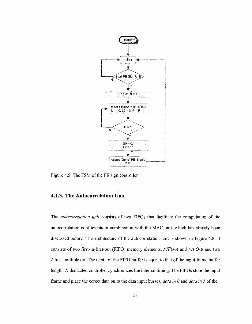
C Reset \ l.llli'iiRMHIIIlig'
Idle
P = 8; N = 1
Reset =1;Sh1 =0;L0 = 0; L1 = 0; L2 = 0; P = P - 1
Assert "Done_PE_Sign" L2 = 0
Figure 4.5: The FSM of the PE sign controller
4.1.3. The Autocorrelation Unit
The autocorrelation unit consists of two FIFOs that facilitate the computation of the
autocorrelation coefficients in combination with the MAC unit, which has already been
discussed before. The architecture of the autocorrelation unit is shown in Figure 4.8. It
consists of two first-in-first-out (FIFO) memory elements, FIFO-A and FIFO-B and two
2-to-l multiplexer. The depth of the FIFO buffer is equal to that of the input frame buffer
length. A dedicated controller synchronizes the internal timing. The FIFOs store the input
frame and place the corect data on to the data input busses, data in 0 and data in 1 of the
57

( Reset \ ,
Assert "Done PE Execution
Figure 4.6: The FSM of the PE execution controller.
58

Data in 0 Data in 1
Reset
C l k - = ^
Data out
Figure 4.7: MAC unit RTL for serial matrix multiplication
x(n)
Data in
Clk 7=i
* * *
1 • n
FIFOB
Control Signals
-• To data bus "Data in 0" of MAC unit
Shift in 2 ^
zfr
-> To data bus "Data in 1" of MAC unit
4— Clk
Figure 4.8: The autocorrelation unit
MAC unit. The autocorrelation coefficients are computed in the MAC unit and are stored
appropriately in the memory unit. The autocorrelation coefficients of the input frame are
computed as follows [71 ]
N-l-m
(m) = y x(n) x{n +ni) m = 0, 1, ... N-l (4.1)
n = 0
59

where r(m) is the autocorrelation coefficient with a lag m and N is the input frame size.
Thus, it can be seen that the autocorrelation coefficient of any lag is computed as the
inner product of a two vectors, the input vector x(m) and the shifted form of the input
vector x(n+m). Implementation of the matrix multiplication is well documented in the
literature and has been described in [27], [72], [73]. The computation of the m'h lag
autocorrelation coefficient requires the shifting of the input vector x(n) m times to form
x(n+m). The delay element in the return path of FIFO-B provides this shift operation.
Thus, with the calculation of each autocorrelation coefficient, the delay element
introduces a shift of one to the input vector. This yields a sufficiently accurate estimate of
the autocorrelation matrix, under the assumption that the signal remains stationary over
the entire frame. The autocorrelation matrix is a canonical arrangement of the
autocorrelation coefficients to form a Toeplitz matrix [74]. The Toeplitz matrix is
diagonalized in the later stages of the speech enhancement processor, which is explained
in Section 4.3.2. The autocorrelation matrix is assumed to be that of either a noise- or a
speech-dominant frame.
The FSM of the autocorrelation controller unit is shown in Figure 4.9. The order of
complexity of computing all the autocorrelation coefficients is 0(n) [75]. The FSM has
been parameterized with variable L, which indicates the length of the input frame and
which is also the size of the input FIFO buffer depth. Other variables such as P and Z,
used in Figure 4.9, are internal counters used by the controller.
60
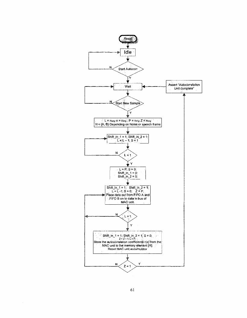
Assert "Autocorrelation Unit complete"
L - norg; n = nbrg ; P - norg; Z = norg
H = {A, B} Depending on Noise or speech frame
I F
_j. Shift in 1 = 1; ——*> L = L -
^
Shift in 2 = 1; 1; S = 1
X L = P;S = 0;
Shift_in_1 = 0; Shift in 2 = 0;
T Shift in_1 = 1; Shift_in_2 = 1;
L = L-1;S = 0; Z=P; Place data out from FIFO A and
FIFO B on to data in bus of MAC unit.
ShiftJnJ = 1; Shift_in_2 = 1; S = 0; Z = Z - 1 : L = P;
Store the autocorrelation coefficients r(z) from the MAC unit to the memory element [H];
Reset MAC unit accumulator
61

Figure 4.9: The FSM of the autocorrelation controller
4.1.4. Eigen-Domain Filter Gain Calculation Unit
The eigen-domain filter has been described in Section 3.3, where the eigen-domain filter
is given by (3.11). The transform is determined by the eigen-vectors while the eigen
values are used for filtering. The eigen-domain filter gain G as described in Section 3.1.1
is a function of the Lagrange parameter and the eigen-values. The Lagrange parameter is
computed adaptively based on the input frame SNR. The Lagrange parameter is given by
(3.13), while (3.14) describes the SNR computation. Figure 4.10 shows the block
diagram of the eigen domain filter, showing the I/O pins of the unit. This unit has I/O
pins, namely, data in, data out, start signal, load control signal L and input threshold
parameter, /uo as an input parameter. The input threshold Lagrange parameter is an
experimentally-set parameter and for our work it is set to 4. Figure 4.11 shows the
architecture of the eigen-domain filter gain unit. It consists of an FIFO buffer of length
equal to that of the input frame size, a 3-to-l MUX, an addition unit and a serial division
unit. The synchronization of each component is maintained by the eigen-domain gain
controller unit through the various control signals. In the first n clocks, the accumulator
computes and holds the summation of the n input data. In the next clock, the value stored
in the accumulator is shifted by an amount of 2~'°82(n). This completes the computation
given by (3.14). In the next clock, this computed value in the accumulator is subtracted
from the value /u0 stored in the register /u0; this completes the computation of (3.13).
Next, the eigen-domain filter parameter G, given by Az(Az + /u I)'', is computed serially
62

in the subsequent clock cycles in combination with the divide unit. The order of
complexity of the serial divide operation is 0(1), where / is the number of bits in each
Threshold input
Data in
Start
Data out
Figure 4.10: The eigen-domain filter (with variable SNR)
Data in BUS
Clk-
SfO - \
1
x(n)
JAin I Clk LI
shift by 2 0 I - *
•log(n)
JUO
a JT IY SO^\MUX / Gain Unit
Controller
Done Div. Done
• Start
Data out BUS
Figure 4.11: The register transfer level (RTL) diagram of the eigen-domain filter
63
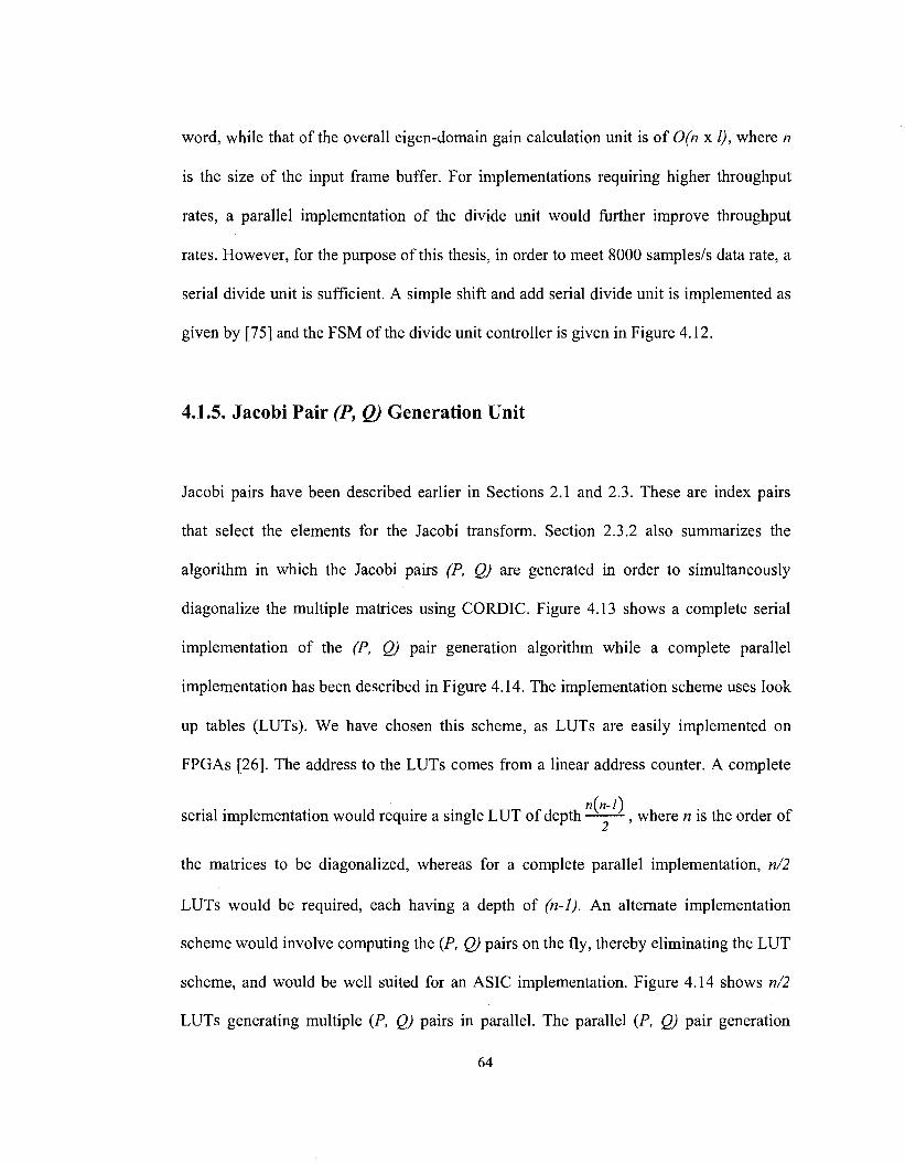
word, while that of the overall eigen-domain gain calculation unit is of 0(n x I), where n
is the size of the input frame buffer. For implementations requiring higher throughput
rates, a parallel implementation of the divide unit would further improve throughput
rates. However, for the purpose of this thesis, in order to meet 8000 samples/s data rate, a
serial divide unit is sufficient. A simple shift and add serial divide unit is implemented as
given by [75] and the FSM of the divide unit controller is given in Figure 4.12.
4.1.5. Jacobi Pair (P, Q) Generation Unit
Jacobi pairs have been described earlier in Sections 2.1 and 2.3. These are index pairs
that select the elements for the Jacobi transform. Section 2.3.2 also summarizes the
algorithm in which the Jacobi pairs (P, Q) are generated in order to simultaneously
diagonalize the multiple matrices using CORDIC. Figure 4.13 shows a complete serial
implementation of the (P, Q) pair generation algorithm while a complete parallel
implementation has been described in Figure 4.14. The implementation scheme uses look
up tables (LUTs). We have chosen this scheme, as LUTs are easily implemented on
FPGAs [26]. The address to the LUTs comes from a linear address counter. A complete
Yl\Yl-l )
serial implementation would require a single LUT of depth —-— , where n is the order of
the matrices to be diagonalized, whereas for a complete parallel implementation, n/2
LUTs would be required, each having a depth of (n-1). An alternate implementation
scheme would involve computing the (P, Q) pairs on the fly, thereby eliminating the LUT
scheme, and would be well suited for an ASIC implementation. Figure 4.14 shows n/2
LUTs generating multiple (P, Q) pairs in parallel. The parallel (P, Q) pair generation
64
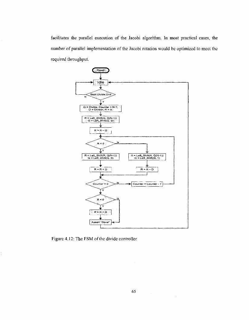
facilitates the parallel execution of the Jacobi algorithm. In most practical cases, the
number of parallel implementation of the Jacobi rotation would be optimized to meet the
required throughput.
C Reset }
Figure 4.12: The FSM of the divide controller
65
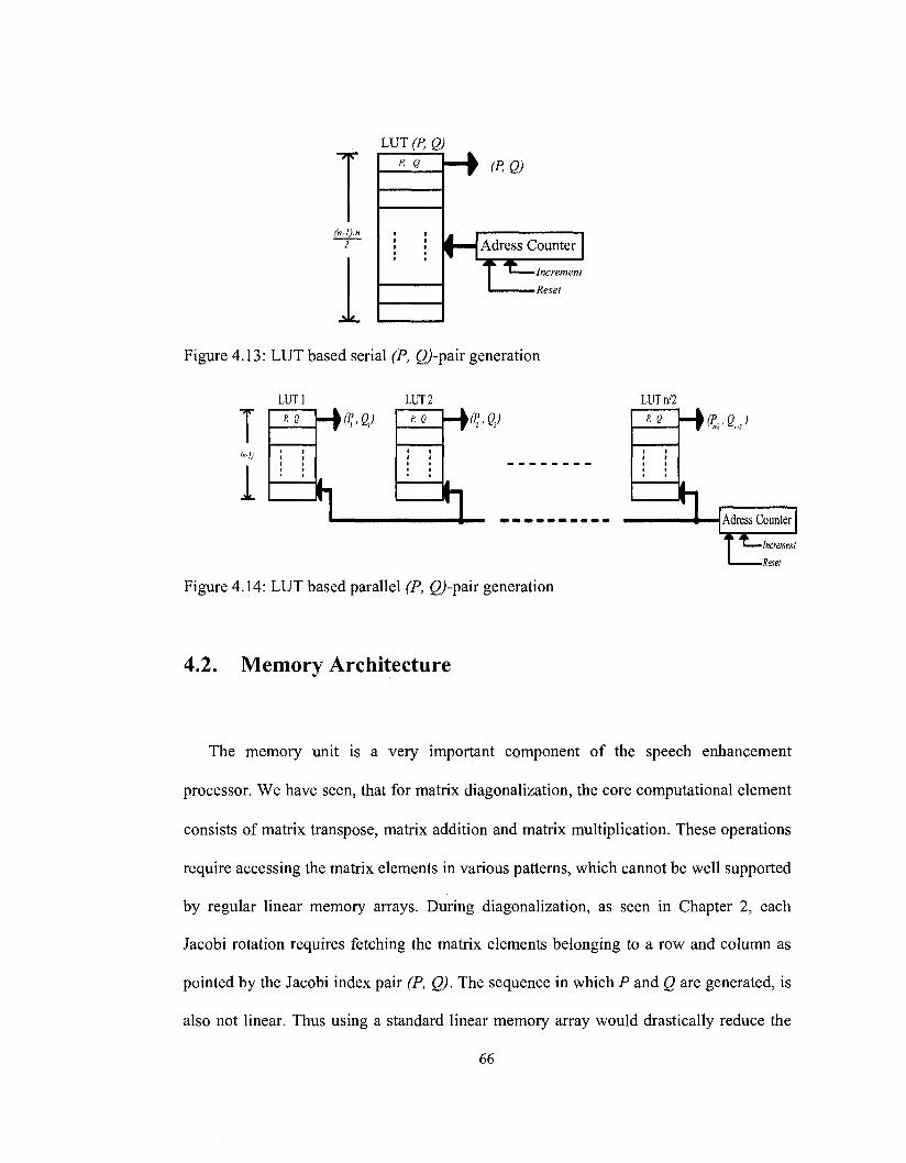
LUT (P, Q) -? r
2
- i c
P. Q — T (p-Q}
Adress Counter 1 Increment
Figure 4.13: LUT based serial (P, 0-pair generation
T (i-i)
1
LUTl LUT 2
r. Q -iv>Q)
h
P. Q -}(P2,Q2)
a Figure 4.14: LUT based parallel (P, gj-pair generation
4.2. Memory Architecture
LUTn/2
f. Q >&.ej
a Adress Counter
TE Increment
Reset
The memory unit is a very important component of the speech enhancement
processor. We have seen, that for matrix diagonalization, the core computational element
consists of matrix transpose, matrix addition and matrix multiplication. These operations
require accessing the matrix elements in various patterns, which cannot be well supported
by regular linear memory arrays. During diagonalization, as seen in Chapter 2, each
Jacobi rotation requires fetching the matrix elements belonging to a row and column as
pointed by the Jacobi index pair (P, Q). The sequence in which P and Q are generated, is
also not linear. Thus using a standard linear memory array would drastically reduce the
66

throughput rate as well as increase the hardware over-head to generate nonlinear
addressing. This is the primary motive behind developing a memory architecture that best
meets the requirements of the diagonalization core. The design of the memory unit is
such that it facilitates the diagonalization process in terms of addressing scheme and also
reduces read/write access time. It is similar to the concept of the transpose memory
developed in [76].
Figure 4.15 shows the I/O block diagram of the dual port multiple row/column shift
memory (DMSM). The DMSM can perform read and write operations at the same time in
two different locations and hence, the name dual port. The idea behind this memory is to
consider it as a vector memory to perform rotation, shift, read and write operations on
selective rows or columns. The DMSM has three standard groups of I/O busses, namely,
data input bus and output data bus, address bus and control bus. Data in and Data out
busses are of width K. The Horr. /Vert, is a 1 bit select line that identifies an operation
either on a row or on a column. The output select bus is the read address of either a row
or a column, as specified by the Horr. /Vert, select line. The output select bus is of width
log2(n), where nxn is the size of the covariance matrices. The shift select bus provides the
address of either a row or a column on which the shift operation is to be performed. The
shift select bus is more like the address bus for the data out bus and the input select bus is
like the address for the data in bus.
4.2.1. DMSM Memory Cell
67
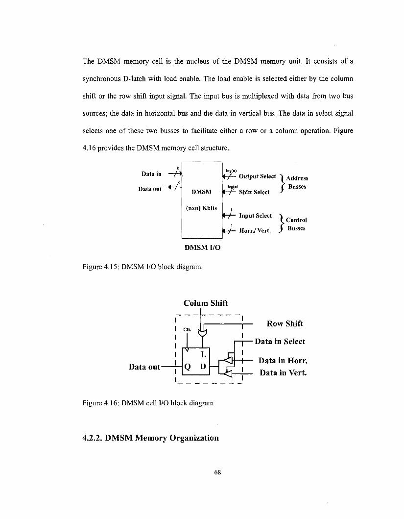
The DMSM memory cell is the nucleus of the DMSM memory unit. It consists of a
synchronous D-latch with load enable. The load enable is selected either by the column
shift or the row shift input signal. The input bus is multiplexed with data from two bus
sources; the data in horizontal bus and the data in vertical bus. The data in select signal
selects one of these two busses to facilitate either a row or a column operation. Figure
4.16 provides the DMSM memory cell structure.
Data in
Data out
log(n)
\-f- Output Select ^Address
iog(n) f Busses DMSM \h-f- Shift Select
(nxn) Kbits Input Select ~\
Horr.
Control
./Vert. ) B u s s e s
DMSM I/O
Figure 4.15: DMSM I/O block diagram.
Colum Shift
Data out
Row Shift
Data in Select
Data in Horr. Data in Vert.
Figure 4.16: DMSM cell I/O block diagram
4.2.2. DMSM Memory Organization
68

The memory organization of the entire DMSM memory is shown in Figure 4.17. It has
nxn DMSM memory cells, two address decoders for row and column decoding, one «-to-
1 multiplexer unit and a few glue-logic. Each DMSM can hold a single nxn matrix at a
time. Due to repetitive structural elements of the DMSM memory cells, the DMSM
memory unit is well suited for ASIC implementation, wherein the DMSM block could be
developed as a hardware hard-macro block. The DMSM has the mechanism to selectively
shift either a row or a column. The DMSM organization is similar to a linear memory
array in terms of the addressing scheme. However, selective row/column shift operation
introduces an extra overhead of a 2-to-l multiplexer in each DMSM memory cell, and
thereby increases the complexity of the DMSM compared to a linear memory array in
[75].
69
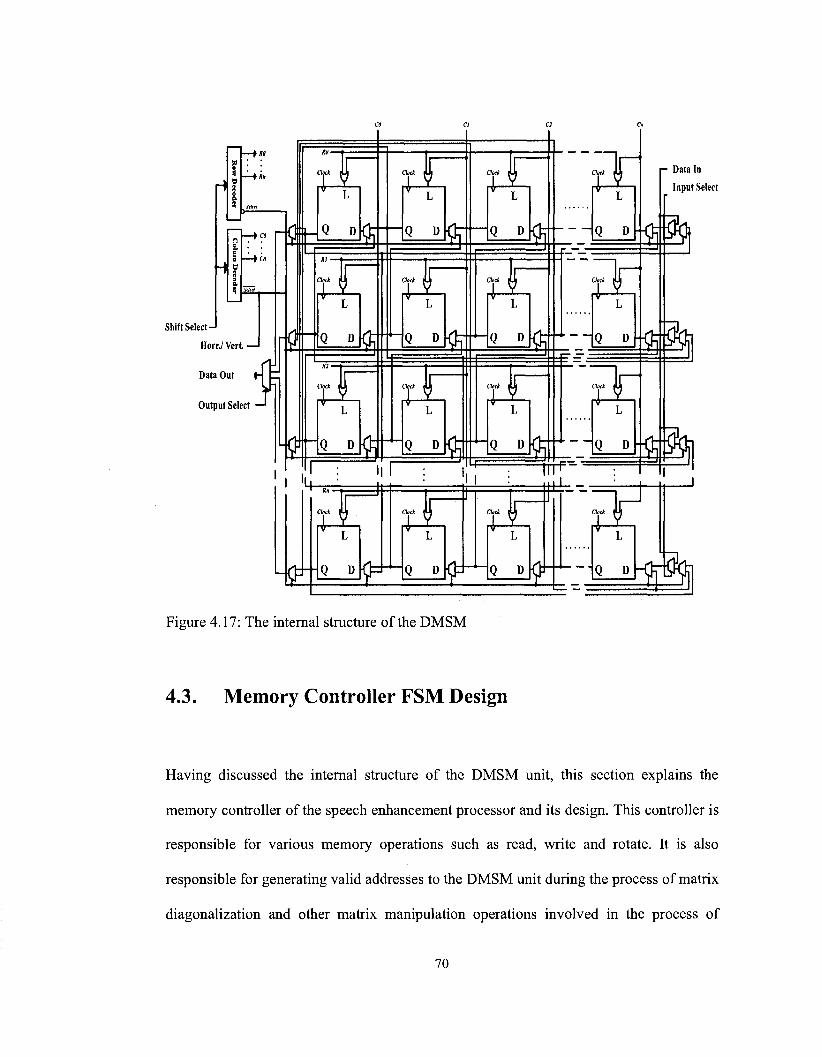
Shift Select
HorrVVert.
Data In
Input Select
Figure 4.17: The internal structure of the DMSM
4.3. Memory Controller FSM Design
Having discussed the internal structure of the DMSM unit, this section explains the
memory controller of the speech enhancement processor and its design. This controller is
responsible for various memory operations such as read, write and rotate. It is also
responsible for generating valid addresses to the DMSM unit during the process of matrix
diagonalization and other matrix manipulation operations involved in the process of
70
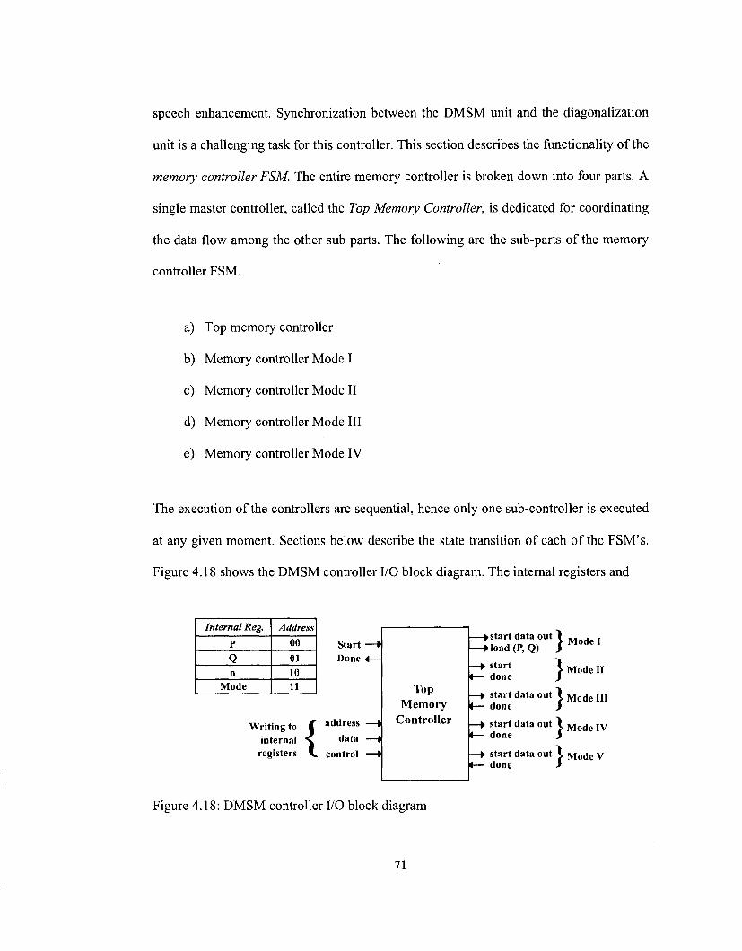
speech enhancement. Synchronization between the DMSM unit and the diagonalization
unit is a challenging task for this controller. This section describes the functionality of the
memory controller FSM. The entire memory controller is broken down into four parts. A
single master controller, called the Top Memory Controller, is dedicated for coordinating
the data flow among the other sub parts. The following are the sub-parts of the memory
controller FSM.
a) Top memory controller
b) Memory controller Mode I
c) Memory controller Mode II
d) Memory controller Mode III
e) Memory controller Mode IV
The execution of the controllers are sequential, hence only one sub-controller is executed
at any given moment. Sections below describe the state transition of each of the FSM's.
Figure 4.18 shows the DMSM controller I/O block diagram. The internal registers and
Internal Reg.
P
Q n
Mode
Address
00
01 10 11
Writing to internal registers {
Start —> Done 4—
dress —t
data —I
ntrol —>
Top Memory
Controller
—•star t data out —Moad(P,Q) J
—> start i— done J
—t start data out 1— done
—t start data out I— done
—• start data out 1— done '-
• Mode I
- Mode II
• Mode III
• Mode IV
> Mode V
Figure 4.18: DMSM controller I/O block diagram
71

their corresponding internal addresses are also shown. The controller is programmed via
the internal registers, namely, P, Q, n and Mode. Registers P and Q hold the Jacobi pairs
(P, Q) for the current operation, while n holds the length of the input frame buffer. The
register Mode displays the present mode being executed by the controller. This is more
like a test register used for testing purpose only. These registers are written and read via
the address, data and control busses used for writing to the internal registers.
4.3.1. Top Memory Controller
The state transition diagram of the Top memory controller is given by Figure 4.19. This
controller synchronizes the other four memory controllers and asserts the "Done Main
memory controller" signal at the end of the execution. The speech enhancement
processor contains three DMSM memory elements, namely, DMSM elements A, B and V.
The covariant matrices that are intended to be diagonalized are stored in DMSM A and B
on a frame-by-frame basis. DMSM A stores the autocorrelation of speech-dominant
frames, while DMSM B stores the autocorrelation of noise-dominant frames. The
computed eigen-vector matrix is stored in DMSM V. Another DMSM element called
DMSM Tmp is used to store an intermediate matrix of size (nxn). The Top memory
controller supervises the execution of each sub-memory controller which are described in
the subsequent sections.
72
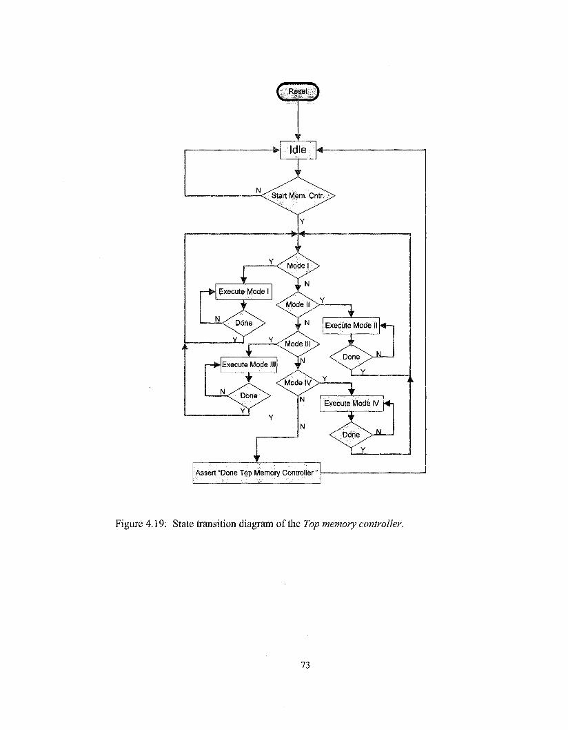
Idle
d$k
Execute Mode iV m-i
Assert "Done Top Memory Controller"
Figure 4.19: State transition diagram of the Top memory controller.
73
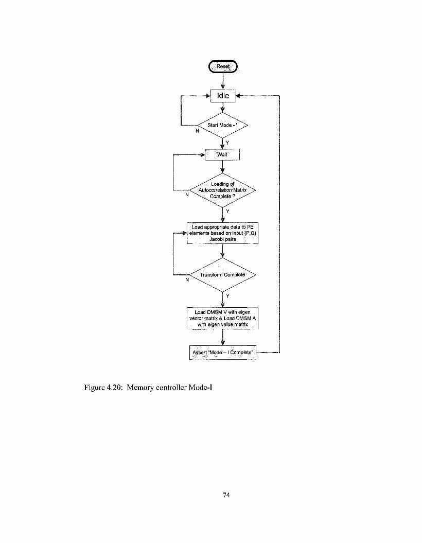
f Reset ^
Idle
Load appropriate data to PE elements based on input (P,Q)
Jacobi pairs
• Load DMSM V with eigen
vector matrix & Load DMSM A with eigen value matrix
Assert "Mode - 1 Complete"
Figure 4.20: Memory controller Mode-I
74
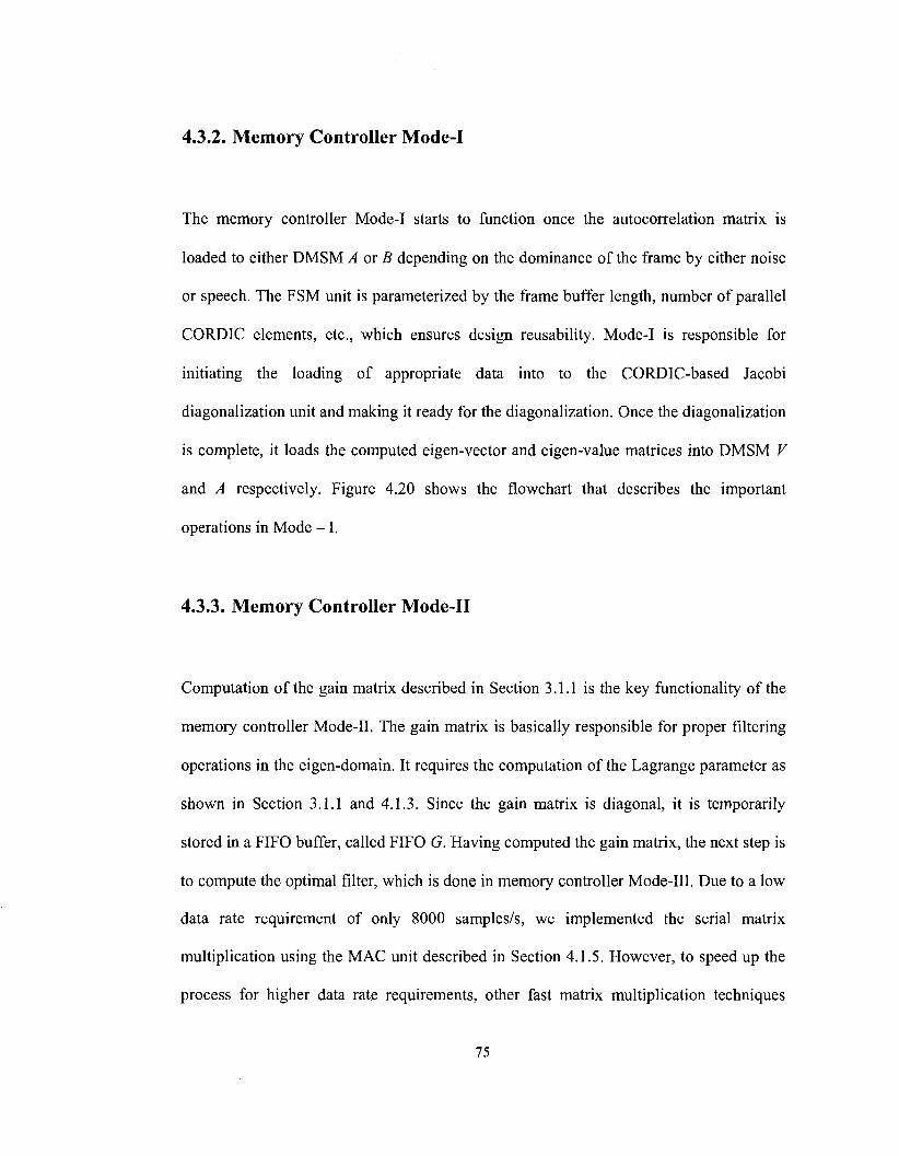
4.3.2. Memory Controller Mode-I
The memory controller Mode-I starts to function once the autocorrelation matrix is
loaded to either DMSM A or B depending on the dominance of the frame by either noise
or speech. The FSM unit is parameterized by the frame buffer length, number of parallel
CORDIC elements, etc., which ensures design reusability. Mode-I is responsible for
initiating the loading of appropriate data into to the CORDIC-based Jacobi
diagonalization unit and making it ready for the diagonalization. Once the diagonalization
is complete, it loads the computed eigen-vector and eigen-value matrices into DMSM V
and A respectively. Figure 4.20 shows the flowchart that describes the important
operations in Mode - 1 .
4.3.3. Memory Controller Mode-II
Computation of the gain matrix described in Section 3.1.1 is the key functionality of the
memory controller Mode-II. The gain matrix is basically responsible for proper filtering
operations in the eigen-domain. It requires the computation of the Lagrange parameter as
shown in Section 3.1.1 and 4.1.3. Since the gain matrix is diagonal, it is temporarily
stored in a FIFO buffer, called FIFO G. Having computed the gain matrix, the next step is
to compute the optimal filter, which is done in memory controller Mode-Ill. Due to a low
data rate requirement of only 8000 samples/s, we implemented the serial matrix
multiplication using the MAC unit described in Section 4.1.5. However, to speed up the
process for higher data rate requirements, other fast matrix multiplication techniques
75
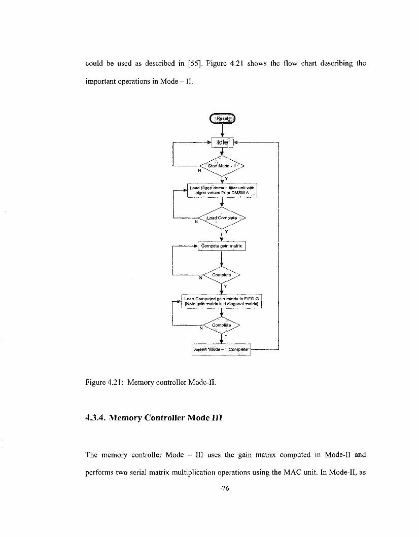
could be used as described in [55]. Figure 4.21 shows the flow chart describing the
important operations in Mode - II.
Load Eigen domain filter unit with eigen values from DMSM A
W Compute gain matrix
Load Computed gain matrix to FIFO G [Note gain matrix is a diagonal matrix]
Assert "Mode - II Complete"
Figure 4.21: Memory controller Mode-II.
4.3.4. Memory Controller Mode III
The memory controller Mode - III uses the gain matrix computed in Mode-II and
performs two serial matrix multiplication operations using the MAC unit. In Mode-II, as
76

the gain matrix was stored in FIFO G, the following operations now take place: Tm/?<—
V. G & G<~ VTY, where DMSM V contains the eigen-vector matrix, FIFO G contains the
diagonal elements of the gain metrix as computed in Mode-II, FIFO Y contains the input
noisy speech vector that is to be enhanced, and DMSM Tmp holds the temporary (nxn)
matrix. Both DMSM A and B are unavailable for storing the temporary matrix. This is
due to the fact that the values stored in DMSM A and B are required for estimating the
next frame autocorrelation. The memory controller Mode - III loads appropriate data on
to the data bus for the MAC unit to perform matrix multiplication and also to store the
computed temporary data back to DMSM Tmp and FIFO G respectively. The stored
matrix in DMSM Tmp and the vector stored in FIFO G are intermediate values and do not
have any specific physical meaning. In Mode - IV, the matrix multiplication of Tmp and
G gives the estimated enhanced speech vectors for the current frame, after which the
entire process repeats for the next speech frame. Figure 4.22 shows the flow chart
describing the operation in Mode - III.
4.3.5. Memory Controller Mode IV
The memory controller Mode-IV computes a serial matrix multiplication operation on
data from DMSM Tmp and FIFO G. Appropriate data is placed on the data bus for the
MAC unit to start the computation. The final output vector is obtained after performing
an overlap-and-add operation with the previous output frame. The resultant vector is the
estimated enhanced speech vector from the noisy speech vector of the current frame.
Figure 4.23 shows the flow chart describing the important operations in Mode - IV.
77
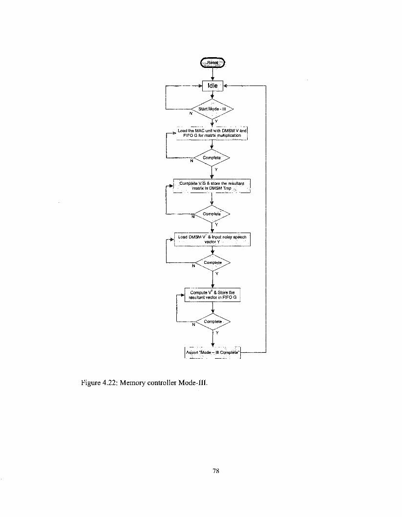
Load the MAC unit with DMSM V and FIFO G for matrix multiplication
Complete V.G & store the resultant matrix in DMSM Tmp
Load DMSM VT & Input noisy speech vector Y
Compute VT & Store the resultant vector in FIFO G
Figure 4.22: Memory controller Mode-Ill.
78

GEO
Load the MAC unit with FIFO G & DMSM Tmp
Compute Tmp.G & store the resultant vector in output buffer
Perform overlap and add operation with previous frame
Assert "Mode - IV Complete"
Figure 4.23: Memory controller Mode-IV.
4.4. Parallel Architecture of the Diagonalization Unit
With the introduction of different hardware elements of the speech enhancement
processor, we now explore the possibilities of parallel implementation of the speech
79
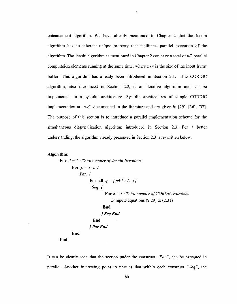
enhancement algorithm. We have already mentioned in Chapter 2 that the Jacobi
algorithm has an inherent unique property that facilitates parallel execution of the
algorithm. The Jacobi algorithm as mentioned in Chapter 2 can have a total of n/2 parallel
computation elements running at the same time, where nxn is the size of the input frame
buffer. This algorithm has already been introduced in Section 2.1. The CORDIC
algorithm, also introduced in Section 2.2, is an iterative algorithm and can be
implemented in a systolic architecture. Systolic architectures of simple CORDIC
implementation are well documented in the literature and are given in [29], [36], [37].
The purpose of this section is to introduce a parallel implementation scheme for the
simultaneous diagonalization algorithm introduced in Section 2.3. For a better
understanding, the algorithm already presented in Section 2.3 is re-written below.
Algorithm: For J = I : Total number of Jacobi Iterations
For p = 1: n-1
Par: {
For all q = {p+l : l:n}
Seq: {
For R = 1 : Total number of CORDIC rotations
Compute equations (2.29) to (2.31)
End
} Seq End End
} Par End End
End
It can be clearly seen that the section under the construct "Par", can be executed in
parallel. Another interesting point to note is that within each construct "Seq", the
80

CORDIC algorithm is executed in order to compute (2.29) to (2.31). As already shown in
[37], the CORDIC systolic architecture further provides scope for increasing the overall
throughput of the system. Figure 4.24 provides a complete parallel implementation
scheme of the algorithm proposed in Section 2.3. Each row computes a single Jacobi
transform given by index pairs (P, Q). Thereby, in a complete parallel implementation
scheme, maximum such possible pairs are N/2. Input to each row is AQ, 2), indicating
matrices Ai and A2 as given by (2.29) to (2.31). As shown earlier in Section 2.2, a total of
R CORDIC iterations complete one single Jacobi rotation, therefore each row in Figure
4.24 comprises of a total of R cascaded PE elements connected in pipeline. Figure 4.24
provides a complete parallel implementation of the proposed algorithm, consuming a
total of RxN PE elements. However, in reality, to ensure the best possible cost effective
implementation, an optimal total number of PE elements are implemented on hardware
by choosing the best number of parallel Jacobi rotations that sufficiently meet the overall
system throughput requirement.
A1,2 (P. Q) 1 •
A,.2(P.&2
PE (0. 0)
PE (0.1)
PE 0. o)
PE (i.i)
-•I PE(R-I.O)
PEm-i. (R-l. I)
- • A;,2(P.Q),
-> A',,2(PQ)2
A I, 2 (P. Q)N/2 • PE (0. N/2) PE (I. N/2) PE, (R-I.N/2) + A-U2(P,Qh
Figure 4.24: Parallel implementation of N/2 Jacobi rotations for a total of R CORDIC
iterations.
81

4.5. The Master Controller
This section integrates all the controllers under a single roof. Figure 4.25 describes
graphically the hierarchical tree of the controllers. This also enables easier testability and
design reusability. The controller, "TOP Controller''' is the supreme controller and is
primarily responsible for synchronization between the rest of the controllers.
4.5.1. TOP Controller Design
The master speech processor controller, Top _Contr oiler is described below. It is
responsible for synchronizing all the blocks. Figure 4.26 shows the FSM of the
Top_Controiler. This controller operates on a frame by frame basis. It is expected that in
a system integration this would intern be controlled by a system controller, which could
either be a microcontroller or a stand-alone controller. The initialization of this controller
is done through the parameter n, which is the size of the input frame buffer.
4.6. Frequency-Subband based Speech Enhancement
Processor
So far we have described the speech enhancement processor that utilizes the simultaneous
diagonalization of two symmetric matrices using CORDIC implementation. We have also
described a technique in Chapter 3, which incorporates an innovative frequency-subband
82
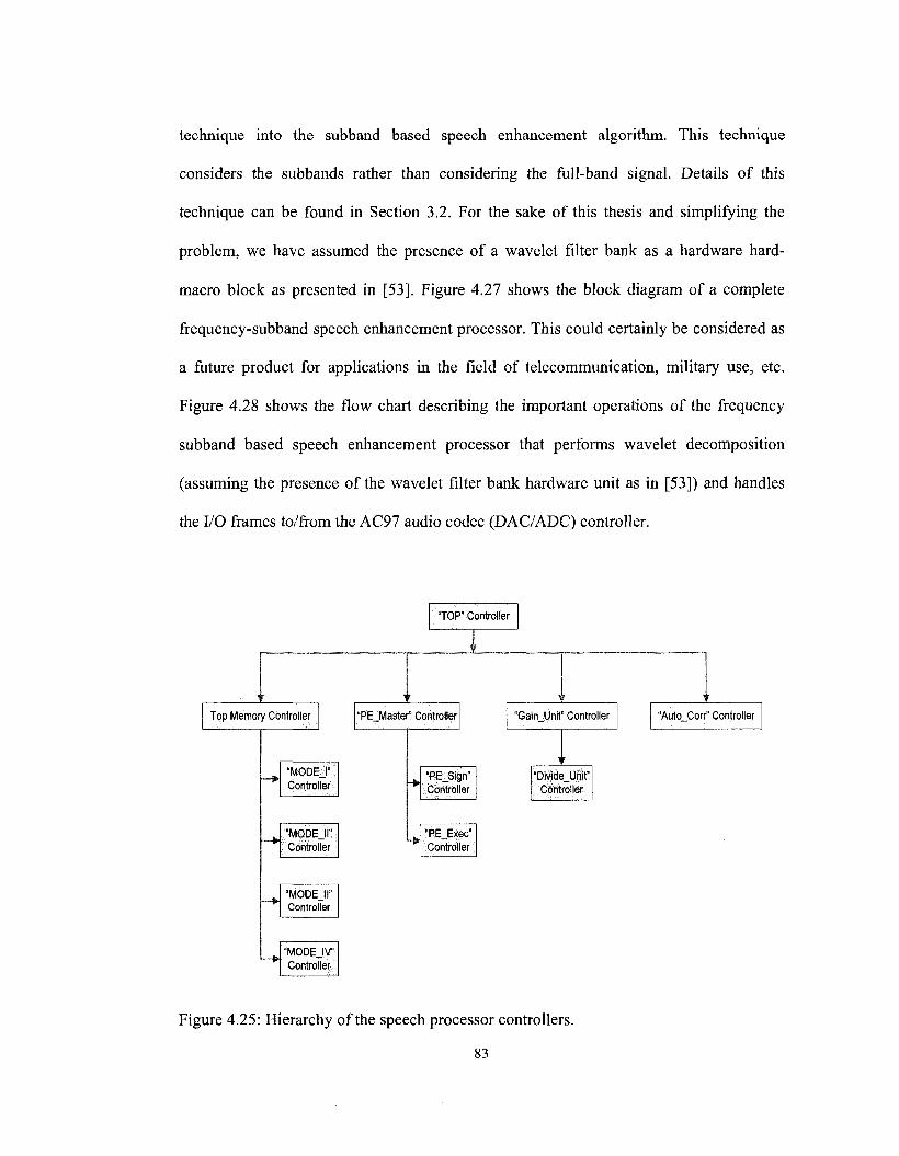
technique into the subband based speech enhancement algorithm. This technique
considers the subbands rather than considering the full-band signal. Details of this
technique can be found in Section 3.2. For the sake of this thesis and simplifying the
problem, we have assumed the presence of a wavelet filter bank as a hardware hard-
macro block as presented in [53]. Figure 4.27 shows the block diagram of a complete
frequency-subband speech enhancement processor. This could certainly be considered as
a future product for applications in the field of telecommunication, military use, etc.
Figure 4.28 shows the flow chart describing the important operations of the frequency
subband based speech enhancement processor that performs wavelet decomposition
(assuming the presence of the wavelet filter bank hardware unit as in [53]) and handles
the I/O frames to/from the AC97 audio codec (DAC/ADC) controller.
Top Memory Controller
~>
- *
_>
— •
"MODEJ" Controller
"MODEJI" Controller
"MODEJI" Controller
"MODEJV" Controller
"TOP" Controller
*PE Master" Controller
*PE_Sign" Controller
"PE_Exec" Controller
"Gain Unit" Controller
'DivideJJnit" Controller
"Auto Corr" Controller
Figure 4.25: Hierarchy of the speech processor controllers.
83
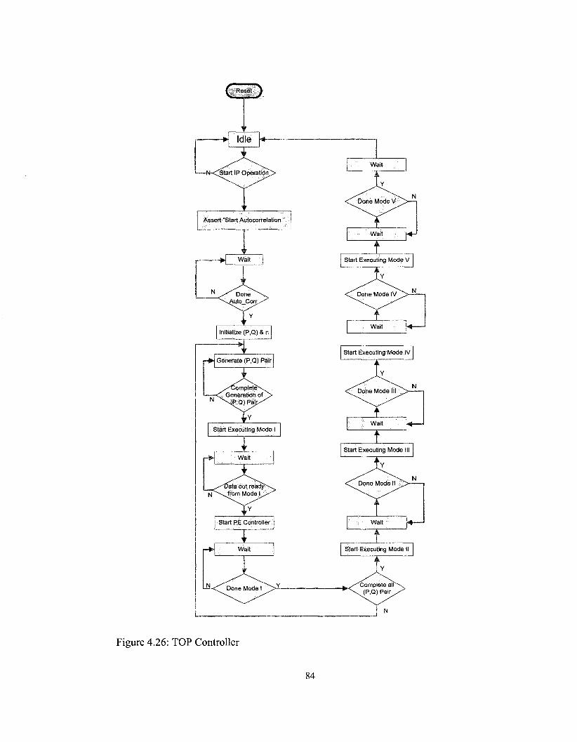
C Reset J
Assert "Start Autocorrelation"
V ait |
Initialize (P,Q) & n
Generate (P,Q) Pair
Start Executing Mode I
Start PE Controller
Wait
Done Mode I
Start Executing Mode IV
Start Executing Mode II
I Y
"'Complete alF" (P,Q)Pair^
N
Figure 4.26: TOP Controller
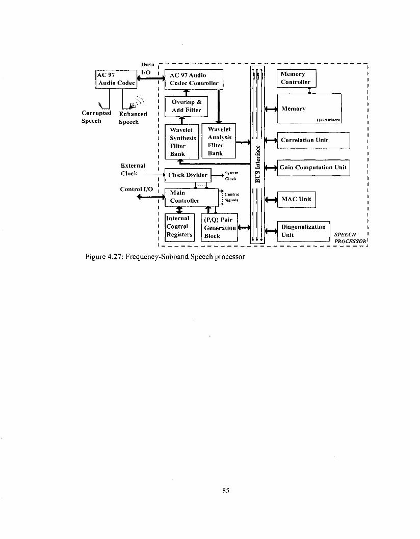
AC 97 Audio Codec
Data I/O
» •
Corrupted Enhanced Speech Speech
External Clock _
Control I/O
AC 97 Audio Codec Controller
Overlap & Add Filter
Wavelet Synthesis Filter Bank
Wavelet Analysis Filter Bank
M Clock Divider
JE3L Main Controller
Internal Control Registers
E
System
Clock
'. Control
: Signals
(P,Q) Pair Generation Block
& PQ
Memory Controller
X
Memory
Correlation Unit
Gain Computation Unit
MAC Unit
Diagonalization Unit SPEECH
PROCESSOR
Figure 4.27: Frequency-Subband Speech processor
85

(Reset /Stop)
Idle
Collect Control & System Parameters (n, N, CORDIC Order, etc)
Collect Input Frame from AC 97 Audio Codec Output buffer
Perform Wavelet Decomposition to get "N" Channels;
Z = N;
•w Collect Frame from Channel "Z"
Compute subspace based Speech Enhancement on
individual subband, "Z"
•
Z = Z - 1
Perform Wavelet Analysis on Channels - 'N '
Perform add and overlap operation
Deliver Output Frame to AC97 audio codec controller output
frame buffer
Figure 4.28: Frequency-Subband Speech Processor.
86

4.7. Summary
In this chapter, we have presented the hardware architecture of the speech enhancement
processor based on the subspace based technique, which we have already described in
Chapter 3. The core of the hardware consists of the diagonalization architecture that best
maps the simultaneous diagonalization of two symmetric matrices described earlier in
Chapter 2. The simultaneous diagonalization architecture is completely multiplier free
making it very attractive for both the FPGA and ASIC implementations. A high performance
dual ported memory has been introduced to best assist the diagonalization core and increase
the overall throughput. The dual port memory increases the throughput of the system by
reducing the complexity of the memory addressing scheme required for matrix manipulation
operations such as, forming a Toeplitz autocorrelation matrix from the autocorrelation
coefficients and performing matrix transpose operations, which otherwise would have
increased the system overhead significantly. The dual port feature of this memory also helps
the concurrent data read and write operations. Finally, we have also presented the
architecture for the frequency subband-based speech enhancement technique. In summary,
this chapter has described the hardware platform for the subspace-based speech enhancement
processor that integrates the simultaneous diagonalization technique described in Chapter 2
and the frequency subband speech enhancement technique described in Chapter 3.
Some of the intricate details of the architecture have also been discussed. To give an
insight into the controllers used and their state machine description, the state transition
diagrams of the significant controllers have been shown. FPGA implementation results of
the architecture in terms of resources utilization and throughput analysis will be presented
in Chapter 5.
87
Chapter 5 : Results & Discussion
So far, we have discussed the CORDIC-based diagonalization technique and its hardware
architecture. We have also seen the utilization of such simultaneous diagonalization
algorithms on a subspace based speech enhancement algorithm. Further, techniques have
been studied to enhance the data rate and reduce complexity by exploring the subband
behavior of the speech signal. In this chapter we present the simulation results and
discussions that confirm the theory developed so far. Results presented in this chapter
include the system level simulation as well as the hardware level simulation.
5.1 System Level Comparison of Speech Enhancement
The process of simultaneous diagonalization has already been described in Chapter 2,
followed by its hardware architecture in Chapter 4. Chapter 3 describes the subspace
based speech enhancement technique. The architecture of the speech enhancement
processor is described in Chapter 4, and is coded in VHDL using the Xilinx ISE design
flow software from Xilinx while the VHDL simulations are performed using the
ModelSim software from Mentor graphics. The Matlab tool from MathWorks is used for
performing all the mathematical calculations and in obtaining the performance measures.
The VHDL model is implemented on a Xilinx FPGA and its resource utilization studied
and presented later in the chapter. The input stimulus to the FPGA is generated from
88
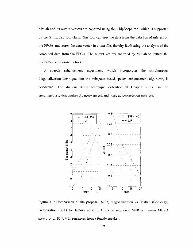
Matlab and its output vectors are captured using the ChipScope tool which is supported
by the Xilinx ISE tool chain. This tool captures the data from the data bus of interest on
the FPGA and stores the data vector in a text file, thereby facilitating the analysis of the
computed data from the FPGA. The output vectors are used by Matlab to extract the
performance measure metrics.
A speech enhancement experiment, which incorporates the simultaneous
diagonalization technique into the subspace based speech enhancement algorithm, is
performed. The diagonalization technique described in Chapter 2 is used to
simultaneously diagonalize the noisy speech and noise autocorrelation matrices.
z 5
I 4 E
A SSF(chol)
* SJR i *
_ M
/ J
i /
: _ -f- _ J
/ l
/
i i
--
Q CO CO
10 15 20 SNR
0.4
0.35
0.3
0.25
0.2
0.15
0.1
0.05
\ \ \ —*—
A J-
\ \ !
V,
SSF(chol)
-SJR
• > s
\ \
... __ \ .. ..\
10 15 SNR
20
Figure 5.1: Comparison of the proposed (SJR) diagonalization vs. Matlab (Cholesky)
factorization (SSF) for factory noise in terms of segmental SNR and mean MBSD
measures of 10 TIMIT sentences from a female speaker.
89

The diagonalization of the covariance matrices of the noisy speech and the noise lead to
the projection of the noisy signal into a signal-plus-noise subspace and a noise subspace.
From these two subspaces, the clean speech is estimated by nulling the signal
components in the noise subspace and retaining the signal subspace. The subspace-based
speech enhancement technique has already been described in Chapter 3. We evaluate the
subspace-based speech enhancement algorithm on 10 TIMIT sentences produced by a
female speaker. Factory noise at various SNR is added linearly from the NOISEX data
base. Figure 5.1 compares the speech enhancement performance measures of the
proposed simultaneous diagonalization technique to that of the Matlab-Cholskey
technique. The performance of the speech enhancement algorithm is observed in terms of
the SSNR and MBSD measures, from the Xilinx FPGA, for speech data sampled at 8
KHz, on a frame size of 32 ms of speech, i.e 256 data points, a Hamming window is
applied with 50% overlap and add. It can be seen from Figure 5.1 that the proposed
simultaneous diagonalization technique, when incorporated in the subspace-based speech
enhancement technique, provides a hardware-friendly multiplier-free implementation
scheme, whose performance results are comparable to that of the Matlab. Achievement of
the computationally efficient hardware system comes with a cost of a slight compromise
in the performance of the speech enhancement. Figure 5.1 shows a minimum deviation of
only 0.5 db in the SSNR measures compared to the Matlab-Cholskey technique, for
factory noise at 20 db, whereas a maximum deviation of 2 db is seen for noise at 5db.
The deviation in performance is seen more at low SNR conditions, whereas in higher
SNR conditions, both the performance of the two algorithms are comparable.
90

5.2 Hardware Implementation Results of Subspace based
Speech Enhancement
Having discussed the overall system performance measures, we now focus on the
feasibility of the speech processor implementation on a FPGA and later project its
feasibility for targeting VLSI implementation. The following sub-sections summarizes
different parameters such as throughput, FPGA resource utilization, total transistor count
and total logic element used. Sections 5.2.1 to 5.2.3 given below describe the throughput
analysis, number of logical elements and total transistor count for the CORDIC based
subspace speech enhancement core. Section 5.2.4 summarizes the specification of the
core.
5.2.1 FPGA Resource Utilization
The proposed CORDIC-based subspace speech enhancement circuit is behaviourally
modelled in VHDL for a 16 bit fixed point data path. A synthesis report on the FPGA
resource utilization and timing constrains of a single PE is given in Tables 5.1, 5.2 and
5.3. The targeted Xilinx FPGA (XC2VP30-7ff896) indicates the average resource
utilization by a single PE to be less than 2% at a clock speed of 117 MHz. Tables 5.1 and
5.3 provide an estimate of the total number of PEs that could be accommodated on a
given FPGA, thereby giving a rough estimate of the total number of PEs that could be
implemented. Table 5.2, on the other hand, provides the maximum achievable system
clock frequency corresponding to the minimum clock period, along with minimum input
91
and output hold time. The meta-stability in flip-flops can be avoided by ensuring that the
data and control inputs are held valid and constant for specified periods before and after
the clock pulse, called the minimum input hold time and the minimum output hold time
respectively. Hence, abiding by the timing summary becomes very crucial in the proper
functioning of the logic circuits. Timing summary report along with FPGA synthesis
report provides valuable information to the system designer and helps in optimally
picking design tradeoffs.
5.2.2 Throughput Analysis
The throughput is defined as the number of signal samples processed by the speech
processor per second. Throughput is a function of the frame buffer size used, total
number of parallel CORDIC based Jacobi elements and the system clock. Figure 5.2
shows the variation of the throughput as a function of various frame buffer size. A
threshold of 8000 samples/s has been marked by the dashed red line to indicate the
minimum throughput requirement. It is clearly seen from the graph that the throughput
increases significantly with the decrease in the frame buffer size. In other words, for a
fixed data rate the flexibility in choosing the number of parallel elements is limited by the
frame buffer size. This is a major design constrain in the CORDIC-based subspace
speech enhancement engine. Figure 5.3 describes the variation of the throughput as a
function of the number of parallel CORDIC based Jacobi elements used, for various
clock frequencies. It clearly shows that a single PE implementation is just not possible to
meet the minimum throughput rate of 8K samples per second for a system clock less than
92
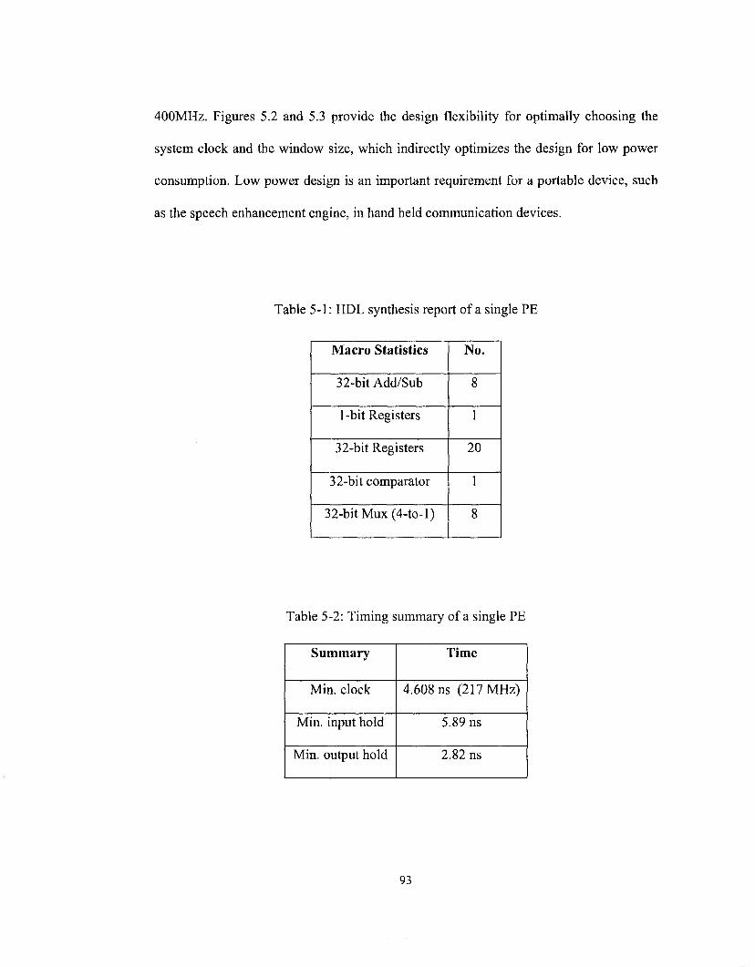
400MHz. Figures 5.2 and 5.3 provide the design flexibility for optimally choosing the
system clock and the window size, which indirectly optimizes the design for low power
consumption. Low power design is an important requirement for a portable device, such
as the speech enhancement engine, in hand held communication devices.
Table 5-1: HDL synthesis report of a single PE
Macro Statistics
32-bit Add/Sub
1-bit Registers
32-bit Registers
32-bit comparator
32-bit Mux (4-to-l)
No.
8
1
20
1
8
Table 5-2: Timing summary of a single PE
Summary
Min. clock
Min. input hold
Min. output hold
Time
4.608 ns (217 MHz)
5.89 ns
2.82 ns

Table 5-3: FPGA resource utilization of a single PE.
Resources
No. of Slice
No. of Slice Flip Flop
No. of4inputLUTs
No. Used
250 out of 13696
110 out of27392
477 out of 27392
Utilized
<2%
< 1 %
<2%
5.2.3 Number of Logic Elements
The number of logic elements used is a very important design parameter. This determines
the total transistor count, routing congestion and the total power consumption. In this
section we examine as to how the design parameters, such as the frame buffer size and
the number of parallel elements that adversely affect the number of logic elements are
being chosen. Figure 5.4 indicates that the number of multiplier elements and the number
of FIFO elements used remain constant for various window sizes. However, the data
memory, which is directly related to the window size grows with the increase in the
window size and almost saturates around the window size of 300 to 400. To maintain a
window size that is power of 2, suitable for generating hardware addressing, we choose a
window size of 256. Figure 5.5 shows the total number of registers required for varying
window size and number of parallel elements used. In Chapter 4, we have seen that the
number of registers in each of the hardware components is linearly dependent on the
window size; hence, as expected, it turns out that the overall register count also obeys
94
linear dependencies with the number of PE elements being used. These graphs assist in
designing for optimal tradeoffs between speed, power and area.
5.2.4 Transistor Count for ASIC Implementation
The implementation of the speech enhancement processor has been done on an FPGA
primarily because of the time constrains. However, the study of the architecture remains
incomplete unless the feasibility of the architecture is studied for an ASIC
implementation. This section, therefore, addresses this issue by studying the estimated
total transistor count for an ASIC implementation of the speech enhancement core. This
also gives a rough estimate of the design complexity. Table 5.4 lists the transistor count
assumed in this thesis for the various logic function used. Transistor count is estimated
based on the area optimized implementation of digital logic circuits which has been
studied in [5]. As described in [5], the cost functions used in Table 5-4 are defined as
( b-\ \ C(a,b) = 4 2YJ(b-i) + 2b-a+]
V i=a ) (5.1)
D(a,b,c) = 2b'a+'xc W
With one of the three inputs to a full adder fixed, (we assume the fixed input is Cin for
convenience, where Q„ is the input carry bit), we have used 12 and 14 transistors for C,„
= 0 and C,„ = 1 respectively, instead of 30 transistors for an ordinary full adder [50]. The
occurrence rates of Q„ = 0 and Q„ = 1 are statistically assumed to be the same as Bc/2
bits out of Bc bits. The adder with subtractor selection needs 8 more transistors for an
95

extra 2-to-l MUX and an inverter compared to that needed for the original full adder as
described in [50].
Figure 5.6 shows the transistor counts as a function of the number of parallel PEs for
various window sizes, keeping the number of CORDIC rotations fixed at 16. Figure 5.7,
on the other hand, shows the transistor counts for various numbers of parallel CORDIC
elements (NPCE), keeping the window size fixed at 256. NPCE indicates the number of
rows in Figure 4.25, i.e., the number of CORDIC operations taking place in parallel. In
custom ASIC design, data memories are normally considered as hard-macros and are
hardcoded pre-defined blocks, which are provided directly by the semiconductor vendors.
These hard-macros are hand layout designs, optimized for area and power consumption.
Hence, the transistor count given in Figures 5.6 and 5.7 are excluding the data memory
and considers minimum length transistors.
5.2.5 Design Specifications
Table 5.5 summarizes the design specification of the CORDIC-based speech
enhancement -processor when implemented on a Xilinx FPGA. A throughput rate of
11600 Samples/s is achieved on a system operating at 200 MHz and a frame buffer size
(window size) of 256 data points. An estimated transistor count of 1158 K makes it
comparable to the 80486 single processor produced by Intel [77], having a total transistor count
of 1200 K and first produced in 1989.
96
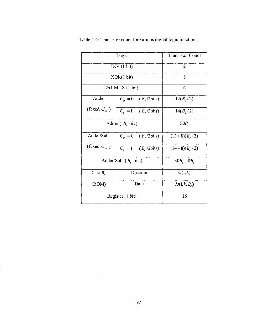
Table 5-4: Transistor count for various digital logic functions.
Logic
INV (1 bit)
XOR(l bit)
2x1 MUX (1 bit)
Adder
(Fixed Cin )
Cin=0 (5c/2bits)
C,,=l (2?c/2bits)
Adder ( Bc bit)
Adder/Sub.
(Fixed Ctn )
C t e=0 (5c/2bits)
C/B=l (5c/2bits)
Adder/Sub. (Bc bits)
2" = Bc
(ROM)
Decoder
Data
Register (1 bit)
Transistor Count
2
8
6
\2(Bc/2)
14(5c/2)
305c
(12 + 8)(5c/2)
(14 + 8)(5c/2)
30BC+SBC
C(\,k)
D(l,k,Bc)
16
97

Window size = 64 % Window size = 91
— * - Window size = 128 Window size = 182
— D - Window size = 256 Window size = 360
— V - Window size = 512 Throughput = 8K Samples/sec
30 40 No. of Parallel PEs
70
Figure 5.2: Throughput vs. the number of parallel PEs used for different window sizes
15 20 No. of Parallel PEs
Figure 5.3: Throughput vs. the number of parallel PEs used for different clock rates.
98
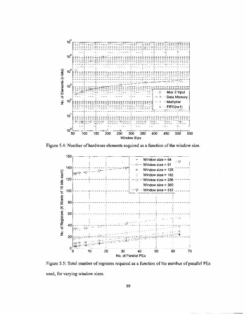
10
10°
£ 10 XI
tn "£ 3 | 10
_D LU
d 10
10'
10"
MM
1 III
M
il
| h ^ - -
1 ±
- -[
: _ _ -^_K^r-rv_T C P S - " " " ^ I
~ 1
!
; _ 5
i—^—*J—-*—
in i
in i
in i
in i
III 1 111 1
III 1
III 1
111 1
1 1 , - - - "
' '' 1 (.
1 1
L 1 t 3
C I
1 ______-1©- - " !
I +
1 1 1 1
1 1 1 1
p : t _
1 1 1 ^ _ L Uf
: : : = =-e*: : - - i : :E: : 1 1
| | 1 (.
L 1 c _t
r~~ i i
! 1 1
__ 1
= = = = = £ * = = = E
I
I
I L tr
= = = = = 1 = =: = =̂ — e — Mux 2 Input
* Data Memory — * - Multiplier —£_ FIFO(nxl)
i
1 1 £ _ _ _ _ }
1 U4f 1
I
| p _
L _ *
50 100 150 200 250 300 350 Window Size
400 450 500 550
Figure 5.4: Number of hardware elements required as a function of the window size.
1 1 to
CO
160
140
120
100
| 80
2> -•— <n
o 6
60
40
20
0
w v -*?-
i
I I
1 I
— *-- - -$-
Window size = 64 Window size = 91
* Window size = 128 e Window size = 182 L3 - Window size = 256
Window size = 360 — V - Window size = 512
I I I I
I I
1 1
i ._ L-.fy
-_=r^#— r — i
i
i i i
j
I
I
- V
- El
- A A -_ *
10 20 30 40 No. of Parallel PEs
50 60 70
Figure 5.5: Total number of registers required as a function of the number of parallel PEs
used, for varying window sizes.
99

4500
4000
3500
3000
2500
2000
1500
1000
500
I I
w ' ^ ; ] J"-
— + — Window size = 64 — $ — Window size = 91
•ft Window size = 128 - i— Window size = 182
— Q - Window size = 256 Window size = 360
— V — Window size = 512
- V
; ;
! _ _ . - £ ]
10 20 30 40 No. of Parallel PEs
50 60 70
Figure 5.6: Transistor count analysis excluding the data memory, as a function of the
number of parallel PEs used, for varying window sizes.
I
1
5000
4500
4000
3500
3000
2500
2000
1500
1000
500
— + - NPCE= 8 — £ — NPCE = 12
— * ~ N P C E = 16 NPCE = 23
— Q - NPCE = 32 NPCE = 46
— V - NPCE = 64
" " " " > "
i — i
i i 57
_ ! _ ^ '
\/ i / i
I I ^ I
T , r "I
J7' \ -\S ' ..!-
! 1 1
i i i i i i
J - n
,- ", '
' i
10 20 30 40 No. of Parallel PEs
50 60 70
Figure 5.7: Transistor count analysis excluding the data memory, as a function of the
number of parallel PEs used, for varying number of parallel CORDIC elements used.
100
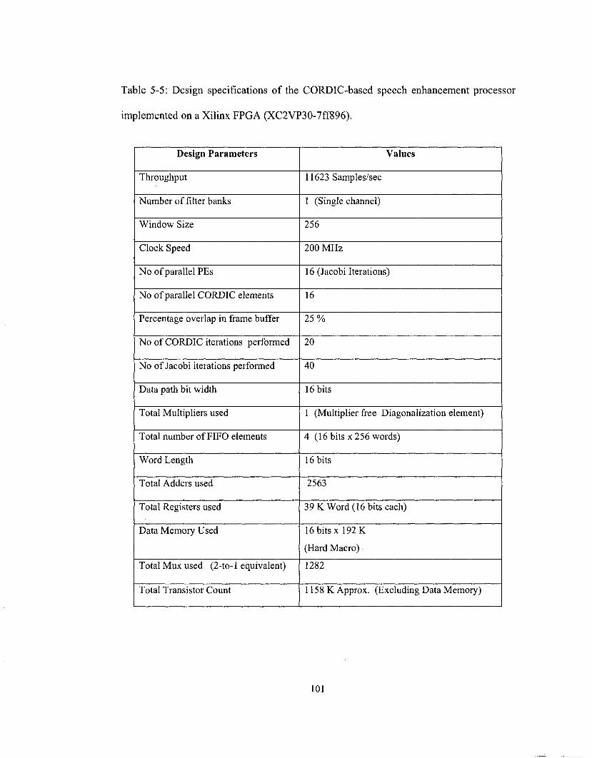
Table 5-5: Design specifications of the CORDIC-based speech enhancement processor
implemented on a Xilinx FPGA (XC2VP30-7ff896).
Design Parameters
Throughput
Number of filter banks
Window Size
Clock Speed
No of parallel PEs
No of parallel CORDIC elements
Percentage overlap in frame buffer
No of CORDIC iterations performed
No of Jacobi iterations performed
Data path bit width
Total Multipliers used
Total number of FIFO elements
Word Length
Total Adders used
Total Registers used
Data Memory Used
Total Mux used (2-to-l equivalent)
Total Transistor Count
Values
11623 Samples/sec
1 (Single channel)
256
200 MHz
16 (Jacobi Iterations)
16
25%
20
40
16 bits
1 (Multiplier free Diagonalization element)
4 (16 bits x 256 words)
16 bits
2563
39 K Word (16 bits each)
16 bits x 192 K
(Hard Macro)
1282
1158 K Approx. (Excluding Data Memory)
101

5.3 Implementation results of the frequency subband
CORDIC- based subspace speech enhancement
The frequency subband technique was introduced in Chapter 3 and the architecture for
the same is subsequently considered in Chapter 4. This section presents the
implementation results of the frequency subband CORIDC-based subspace speech
enhancement processor. Implementation in terms of the FPGA resource utilization,
throughput analysis, number of logic elements used and the total transistor count results
is studied.
5.3.1 FPGA Resource Utilization
The resource utilization of the FPGA (XC2VP30-7ff896) for an NxM processor size is
given in Tables 5.6, excluding the data memory unit, where N represents the number of
frequency-subbands and M the number of parallel elements. Tables 5.7 provide the
timing summary of Table 5.6 for a 16 bit data path.
5.3.2 Throughput Analysis
This section shows the dependency of throughput on increasing number of frequency-
subbands, i.e., the number of filter banks. NPE indicates the number of parallel
processing units. Figure 5.8 presents the net throughput analysis for varying number of
filter banks. It can be clearly seen that the maximum gain in throughput is up to a
102
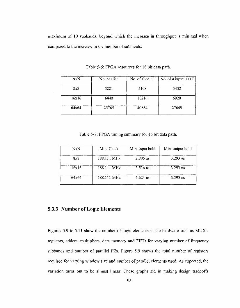
maximum of 10 subbands, beyond which the increase in throughput is minimal when
compared to the increase in the number of subbands.
Table 5-6: FPGA resources for 16 bit data path.
NxN
8x8
16x16
64x64
No. of slice
3221
6440
25765
No. of slice FF
5108
10216
40864
No. of 4 input LUT
3452
6920
27649
Table 5-7: FPGA timing summary for 16 bit data path.
NxN
8x8
16x16
64x64
Min. Clock
188.111 MHz
188.111 MHz
188.111MHz
Min. input hold
2.805 ns
3.516 ns
5.624 ns
Min. output hold
3.293 ns
3.293 ns
3.293 ns
5.3.3 Number of Logic Elements
Figures 5.9 to 5.11 show the number of logic elements in the hardware such as MUXs,
registers, adders, multipliers, data memory and FIFO for varying number of frequency
subbands and number of parallel PEs. Figure 5.9 shows the total number of registers
required for varying window size and number of parallel elements used. As expected, the
variation turns out to be almost linear. These graphs aid in making design tradeoffs
103

between the speed, power and area. Figure 5.10 shows the total number of adders
required for varying filter bank size and number of parallel CORDIC elements. Figure
5.11 shows the variation in the 2-to-l MUX, multiplier and FIFO required as a function
of the number of parallel elements.
5.3.4 Transistor Count for ASIC Implementation
The total transistor count estimate is shown in Figures 5.12 and 5.13. Table 5-4 has
already presented the transistor count estimates of the individual blocks. Figure 5.12
studies the transistor count dependencies for varying number of filter banks and number
of parallel PEs. Figure 5.13, on the other hand, shows the transistor counts for various
numbers of parallel CORDIC elements (NPCE). This once again presents another view of
the design feasibility for ASIC implementations. However, importing a design from an
FPGA to an ASIC implementation would require optimization in several dimensions such
as the ASIC technology to be used, transistor routing and power estimation, and this is
beyond the scope of this thesis. Hence, only an estimate of an ASIC feasibility is
projected via the total transistor count. Transistor count shown in Figure 5.12 excludes
the data memory and assumes the presence of hard-macro memory blocks.
104
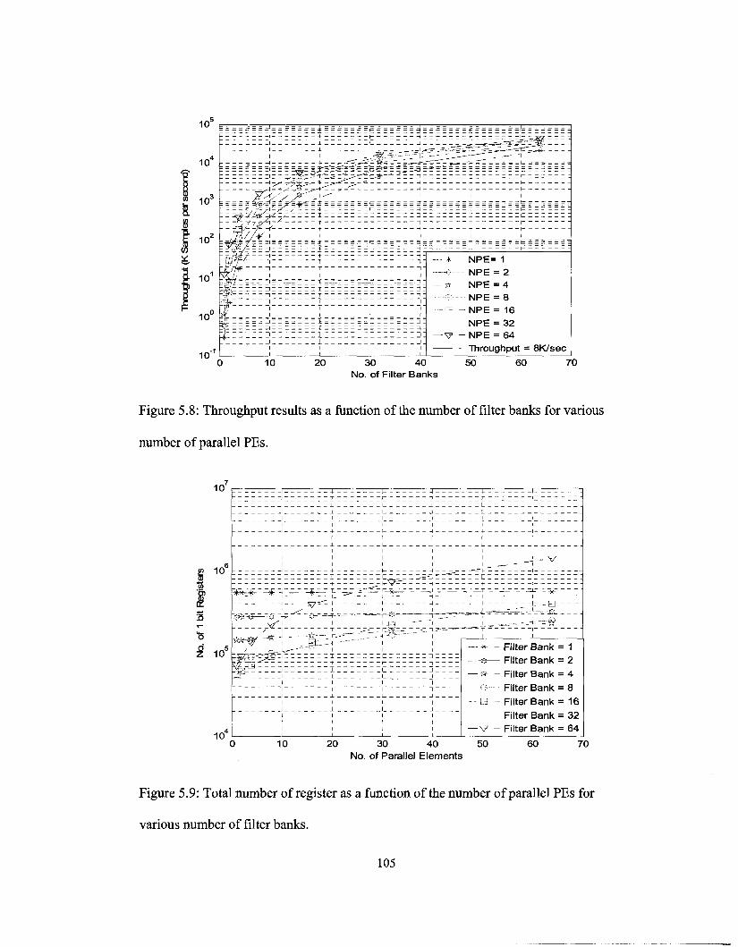
30 40 No. of Filter Banks
Figure 5.8: Throughput results as a function of the number of filter banks for various
number of parallel PEs.
10
10
i 10°
10"
I I I I I I
1 + [ 1 ) 1
I I I I I I
I I I I I I
- I + l - V ~ ~ H <- 1 - :
- * * - * - — £ -L — - * • — t —^ = — i-^f - — 3 - — - — t _ — _ _ i _ — ^
1 5^^: | __ 1 j . _ _ _. _,_. -__&.
C & " ! ? $ — H . -C 1 — T - T - J
c f^ i i i i
1 1 1 1 1 1 1 1 1 1 1 1
1 1
— +- - Filter Bank = 1
— * - Filter Bank = 4 G Filter Bank = 8 Q Filter Bank = 16
Filter Bank = 32
— V - Filter Bank = 64
10 20 30 40 50 No. of Parallel Elements
60 70
Figure 5.9: Total number of register as a function of the number of parallel PEs for
various number of filter banks.
105
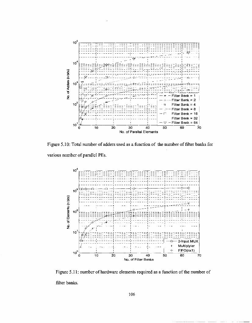
(0
& c
— *- - Filter Bank = 1 Filter Bank = 2
— * - Filter Bank = 4 --—e— Filter Bank = 8 — E - Filter Bank = 16
Filter Bank = 32 — V - Filter Bank = 64
20 30 40 50 No. of Parallel Elements
70
Figure 5.10: Total number of adders used as a function of the number of filter banks for
various number of parallel PEs.
B c
w •8
mJ
102
101
i n "
£©-© ©—
T> - if-0.
7
-±~ -- t 1 1
— _j 1
t 1 1
I I I I
1
_ +
i J = J _
1 i
1 1
1
^ I I I I
- 4 -
~ T
1 i
-------z^-zz
1
1
l
l -l
T
^ ^ I - " " I I I
-J? - r
i
- -+• —
- 1 —
_ + _ _
1
! 1 1 1
1
1 1
T I I
I I t I I I
1
1 1
1
+•
— © — 2-
, Q
_—-£
- 4
nput MUX * MultiDlvier
rO(nx1)
10 20 30 40 No. of Filter Banks
50 60 70
Figure 5.11: number of hardware elements required as a function of the number of
filter banks.
106
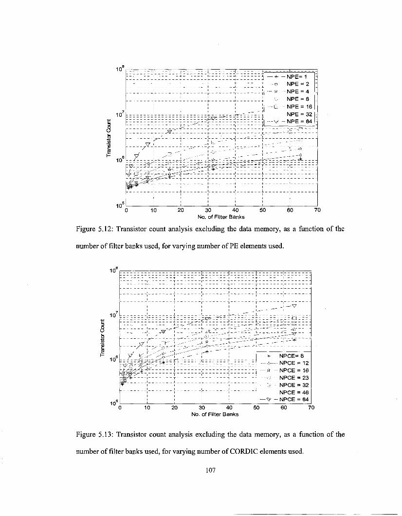
--*- - N P E = 1 ---$- NPE = 2
* - N P E = 4 O NPE = 8 Ld - NPE = 16
NPE = 32 V - N P E = 64
30 40 No. of Filter Banks
Figure 5.12: Transistor count analysis excluding the data memory, as a function of the
number of filter banks used, for varying number of PE elements used.
&
1 + NPCE= 8 •*--••• NPCE = 12 if - N P C E = 16
NPCE = 23 — 3 - NPCE = 32
NPCE = 46 — V - NPCE = 64
30 40 No. of Filter Banks
70
Figure 5.13: Transistor count analysis excluding the data memory, as a function of the
number of filter banks used, for varying number of CORDIC elements used.
107
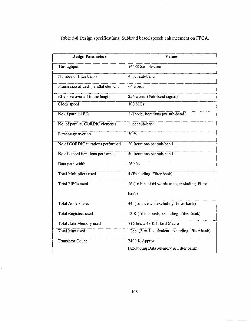
Table 5-8 Design specifications: Subband based speech enhancement on FPGA.
Design Parameters
Throughput
Number of filter banks
Frame size of each parallel element
Effective over all frame length
Clock speed
No of parallel PEs
No. of parallel CORDIC elements
Percentage overlap
No of CORDIC iterations performed
No of Jacobi iterations performed
Data path width
Total Multipliers used
Total FIFOs used
Total Adders used
Total Registers used
Total Data Memory used
Total Mux used
Transistor Count
Values
14488 Samples/sec
4 per sub-band
64 words
256 words (Full-band signal)
100 MHz
1 (Jacobi Iterations per sub-band)
1 per sub-band
50%
20 Iterations per sub-band
40 Iterations per sub-band
16 bits
4 (Excluding Filter bank)
16 (16 bits of 64 words each, excluding Filter
bank)
44 (16 bit each, excluding Filter bank)
12 K (16 bits each, excluding Filter bank)
(16 bits x 48 K) Hard Macro
1288 (2-to-l equivalent, excluding Filter bank)
2400 K Approx
(Excluding Data Memory & Filter bank)
108

5.3.5 Design Specifications
Table 5-8 summarizes the design specifications of the frequency subband processor. A
throughput of 14488 samples/s has been achieved on a system operating at 115 MHz. An
estimated transistor count of 2400 K makes it comparable to the Pentium processor
produced by Intel in 1993 to have a total transistor count of 3100 K [77].
5.4 Summary
This chapter has presented the reader with the FPGA implementation results of the
subspace-based speech enhancement algorithms that have already been presented in
Chapters 2 and 3. The initial part of this chapter presented the overall system
performance measures in terms of the SSNR and MBSD. The design has been
categorized into two parts, the full band version of the CORDIC-based subspace speech
processor and the frequency-subband CORDIC based subspace speech processor. The
later part of this chapter presented the design tradeoffs in implementing the processor on
an FPGA. Important design parameters such as the throughput and the number of logic
elements were presented for varying number of filter banks, number of parallel PEs,
frame buffer size (Window size) and the system clock. A projection of the feasibility of
the VLSI implementation of the design has also been shown in terms of the transistor
count. Design specifications of both the full band and subband designs have been given.
It has been observed that the VLSI implementation of the speech enhancement processor
109
based on a very high number of subbands become impractical; similarly, achieving a very
high throughput rate also becomes impractical in the pure full band implementation. An
optimum design would, therefore, pick the most suitable number of subbands to equally
take advantage of the increase in throughput rate and retain the implementation feasibility
in terms of the hardware overhead due to the subbands. This gives us the freedom to
optimize the design parameters and this could be studied as part of future work.
110
Chapter 6 : Conclusion
In this thesis, we have explored the simultaneous matrix diagonalization of a number of
symmetric matrices keeping in mind the hardware implementation issues. As an
application, we have considered the subspace based speech enhancement problem. Later,
it has been shown that the use of subband processing enhances the overall system
performance and also increases the overall system throughput. This has enabled the
processing of data at a much higher sampling rate compared to the full-band
implementation. Due to time limitations of the thesis, only an FPGA implementation has
been studied and a projection of the transistor count has been made for an ASIC
implementation.
6.1. Conclusion and Thesis Summary
We have presented an innovative technique for simultaneous diagonalization of multiple
symmetric matrices to address the emerging popularity of the eigen-domain signal
processing technique in realtime. The proposed technique has been based on the Jacobi
rotation of matrices using the CORDIC iterative approach. Due to the simplicity of its
computational elements such as shift-and-add, the architecture becomes ideally suited for
targeting FPGA/ASIC implementation. The proposed diagonalization technique has
shown better results as compared with that of the Matlab-Cholesky factorization. It has
111
been demonstrated that the system performance of the speech enhancement processor is
at par with the overall system performance achieved from Matlab simulation, using the
Matlab-Cholskey factorization method, in the presence of reasonable noise conditions.
A subband-based speech enhancement analysis technique, which exploits the slow
varying characteristics of the speech and noise signals over narrow frequency segments,
has also been proposed. The accurate covariance estimation of the noise and speech in the
subbands has resulted in a better performance under low SNR conditions as compared to
that of the full band subspace-based speech enhancement technique. The proposed
technique also provides an inherent parallel implementation scheme and reduces the
computational complexity. The proposed scheme makes no assumptions of the spectral
characteristics of the noise, but only assumes that the noise and speech are uncorrelated
in each of the subbands.
In the later part of the thesis, we have presented the hardware architecture along with
simulation results. System level simulations have been performed to highlight the
performance gain along with hardware implementation results. The speech enhancement
processor has been implemented both for the full band and the subband algorithms. Also,
a projection of the processors ASIC counterpart has been suggested from the transistor
count point of view.
112
6.2. Future Work
Some of the areas for future development are as follows:
• ASIC implementation of the proposed simultaneous diagonalization technique for
high data-rate applications such as software defined radio and video applications
involving de-noising issues.
• A custom ASIC implementation would certainly attract more attention from
industry in using the subspace-based speech enhancement for commercial use.
• Various other techniques such as incorporating fast number systems such as the
residue number system could further increase the throughput.
• Considering various noise models and predefined templates of the noise
autocorrelation matrices would boost the overall system performance. This would
provide a better autocorrelation estimate of the noise, which is the key to a better
speech enhancement performance.
113

References
[1] G. S. Sarkar, "Speech science modeling for automatic accent and dialect
classification" PhD Thesis, University of Colorado at Boulder, 2007.
[2] D. O'Shaughnessy, "Speech Communication: Human and Machine" 2nd edition,
Wiley-IEEE Press 1999.
[3] V. Zummeren and I. James, "A speech communication course concept for
Marine Corps Command and Staff College in partnership with Northern Virginia
Community College-Woodbridge", PhD Thesis, George Mason University,
2004.
[4] E. Moreau, "A generalization of joint diagonalization criteria for source
separation", IEEE Trans. Signal Process. Vol. 49, pp. 530-541, March 2001.
[5] B. Yang, "Projection approximation subspace tracking," IEEE Trans. Signal
Processing, Vol. 43, No. 1, pp. 95-107, Jan. 1995.
[6] B. Cernuschi-Frias, S.E. Lew, H. J. Gonzalez and J. D. Pfefferman, "A parallel
algorithm for the diagonalization of symmetric matrices", Proc. IEEE Int.
Symposium on Circuits and Systems, ISCAS-2000, Vol. 5, pp. 81-84, May 2000.
[7] B. N. Flury, "Common principle components in k groups", J. Amer. Statist.
Assoc, Vol. 79, pp. 892-897, 1984.
[8] J. F. Cardoso and A. Souloumiac, "Blind beamforming for non Gaussian
signals, " Inst. Elect. Eng. Proc. F, Vol. 140, no. 6, pp. 362-370, 1993.
114

[9] A. Belouchrani, K. Abed Meraim, J. F. Cardoso, and E. Moulines, "A blind
source separation technique based on second order statistics," IEEE Trans.
Signal Process., vol. 45, no. 2, pp. 434-444, Feb. 1997.
[10] O. J. Micka and A. J.Weiss, "Estimating frequencies of exponentials in noise
using joint diagonalization," IEEE Trans. Signal Process., Vol. 47, no. 2, pp.
341-348, Feb. 1999.
[11] L. De Lathauwer, B. De Moor and J. Vandewalle, "Independent component
analysis and (simultaneous) third-order tensor diagonalization", IEEE Trans.
Signal Process. Vol. 49, No. 10, pp. 2262-2271, 2001.
[12] P. Gruber, F.J Theis, K. Stadlthanner, E.W. Lang, A.M Tome and A.R Teixeira,
"Denoising using local ICA and kerael-PCA", Proc. IEEE Int. Conf. Neutal
Networks, Vol. 3, pp. 2071 - 2076, July 2004.
[13] S. F. Hsiao, "Adaptive Jacobi method for parallel singular value
decompositions", Proc. IEEE Int. Conf. Acoust., Speech and Signal Processing,
ICASSP-95, Vol. 5, pp. 3203-3206, May 1995.
[14] M. Alonso, G. Richard and B. David, "Accurate tempo estimation based on
harmonic + noise decomposition", EURASIP Journal on Advances in Signal
Proc, Vol. 2007, Article ID 82795, 2007.
[15] B. Champagne and Q. G. Liu, "Plane rotation-based EVD updating schemes for
efficient subspace tracking", IEEE Trans. Signal Process. Vol. 46, pp. 1886-
1900, July 1998.
115
[16] B. Champagne and Q. G. Liu, "A New Family of EVD Tracking algorithms
using givens rotations", Proc. IEEE Int. Conf. Acoust, Speech and Signal
Processing, ICASSP-96, Vol. 5, pp. 1-4, May 1996.
[17] X. L. Li and X. D. Zhang, "Nonorthogonal Joint Diagonalization Free of
Degenerate Solution", IEEE Trans. Signal Process. Vol. 55, pp. 1803-1814, May
2007.
[18] M. Wax and J. Sheinvald, "A least-squares approach to joint diagonalization,"
IEEE Signal Process. Lett, Vol. 4, no. 2, pp. 52-53, Feb. 1997.
[19] Y. Ephraim and H. L. Van Trees, "A signal subspace approach for speech
enhancement," IEEE Trans. Speech and Audio Processing, Vol. 3, pp. 251-266,
July 1995.
[20] Y. Hu and P.C. Loizou,"A generalized subspace approach for enhancing speech
corrupted by colored noise," IEEE Trans. Speech and Audio Processing, Vol.
ll,pp.334-341, July 2003.
[21] Y. Hu and P.C. Loizou, "Speech enhancement based on wavelet thresholding the
multitaper spectrum," IEEE Trans. Speech and Audio Processing, Vol.
12, pp.59-67, Jan 2004.
[22] F. Jabloun and B. Champagne,"Incorporating the human hearing properties in
the signal subspace approach for speech enhancement", IEEE Trans. Speech and
Audio Processing, Vol. 11, Issue 6, pp.700-708, Nov. 2003.
[23] M. Bahoura and J. Rouat, J, "Wavelet speech enhancement based on the Teager
energy operator," IEEE, Signal Processing Lettr, Vol. 8, pp. 10-12, Jan. 2001.
116
[24] J. A.B. Fortes, "Future challenges in VLSI system design", Proc. IEEE
Computer Society Annual Symposium, pp. 5-7, Feb, 2003.
[25] P. Sinha, D. Basu and A. Sinha: "A Novel Architecture of a Reconfigurable
Parallel DSP Processor" IEEE Int. Proc. NEWCAS 2005, July, 2005.
[26] Xilinx, "Introduction and overview", Virtex-II Pro Platform FPGAs, March 9th,
2004.
[27] G.H. Golub and C.F. Van Loan, "Matrix Computations", 3rd edition, Johns
Hopkins University Press, 1996.
[28] S.B. Searle, Matrix Algebra Useful for Statistics. New York: Wiley, 1982.
[29] J. Vails, M. Kuhlmann and K.K Parhi, "Efficient mapping of CORDIC
algorithms on FPGA", IEEE Workshop on Sig. Procc. Sys., 2000, pp. 336 - 345,
Oct. 2000.
[30] J.H. Wilkinson, "Note on the Quadratic Convergence of the Cyclic Jacobi
Process" Numer. Math. 6, 296-300, 1962.
[31] J.W. Demmel and K. Veselic, "Jacobi's Method is More Accurate than QR",
SIAMJ. Matrix Anal. Appl., Vol. 13, pp. 1204-1245, 1992.
[32] J.H. Wilkinson, "The Algebraic Eigenvalue Problem", London, Oxford Univ.
Press, 1965.
[33] J. E. Voider, 'The CORDIC trigonometric computing technique", IRE Trans.
Electron. Comput, Vol. EC-8, pp. 330-334, Sept. 1959.
[34] J. S. Walter, "A Unified View of CORDIC Processor Design", Application
Specific Processors, Edited by Earl E. Swartzlander, Jr., pp. 121-160, Kluwer
Academic Press, Nov. 1996.
117
[35] Yi Yang, "A Distributed Arithmetic Based CORDIC Algorithm and its Use in
the FPGA Implementation of 2-D IDCT", M.A.Sc Thesis, Concordia University,
April 2002.
[36] C. H. Lin and A. Y. Wu, "Mixed-scaling-rotation CORDIC (MSR-CORDIC)
algorithm and architecture for high-performance vector rotational DSP
applications", IEEE Trans, on Circuits and Systems, Vol. 52, no. 11, pp. 2385-
2396, Nov. 2005.
[37] R. Andraka, "A survey of CORDIC algorithms for FPGA based computers",
Proc. ACM/SIGDA sixth International Symposium on Field Programmable, pp.
191-200, 1998.
[38] S. Wang, "A CORDIC Arithmetic Processor", PhD Thesis, University of Texas
at Austin, May 1998.
[39] T. Painter and A. Spanias, "Perceptual coding of digital audio", Proc. IEEE, Vol.
88, Issue 4, pp. 451 -515, April 2000.
[40] W. Yang, M. Benbouchta and R. Yantorno, "Performance of the modified Bark
spectral distortion as an objective speech quality measure" Proc. IEEE Acoustics,
Speech, and Signal Processing ICASSF'-98, Vol. l,pp. 541-544, 1998.
[41] Zwicker, E., "Subdivision of the audible frequency range into critical bands,"
The Journal of the Acoustical Society of America, Feb., 1961.
[42] P. Sinha, M.N.S. Swamy, P.K. Meher, "FPGA Implementation of Fast
Simultaneous Diagonalization of matrices for subspace based speech
enhancement", IEEE Int. Proc. MWSCAS, August, 2007.
118

[43] C. H. You, S. Rahardja, S. N. Koh, "Audible Noise Reduction in Eigendomain
for Speech Enhancement", IEEE Trans, on Audio, speech and language Procc,
Vol. 15, pp 1753-1765, Aug, 2007
[44] P. Sinha, S. Sarkar, A. Sinha, D. Basu, "Architecture of a Configurable Centered
Discrete Fractional Fourier Transform Processor", IEEE Int. Proc. MWSCAS,
August, 2007.
[45] C.H You, S. N. Koh and S. Rahardja,"Signal Subspace Speech Enhancement for
Audible Noise Reduction" Proc. IEEE Acoustics, Speech, and Signal
Processing, ICASSP 05, Vol. 1, pp. 145-148, 2005.
[46] P. Sinha, A. Sinha and D. Basu: "Reconfigurable Single Function Multiple Data
(SFMD) Architecture for a Class of Signal/Image Processing Applications"
IEEE Workshop on Circuits and Systems for 4G Mobile Wireless
Communications, pp 46-49, June, 2005.
[47] Y. Hu and P.C. Loizou, "A perceptually motivated approach for speech
enhancement," IEEE Trans. Speech and Audio Processing, Vol. 11, pp.457-465,
Sept. 2003.
[48] F. Jabloun and B. Champagne, "A Perceptual Signal Subspace Approach for
Speech Enhancement in Colored Noise," Proc. IEEE Int. Conf. Acoust., Speech
and Signal Processing, ICASSP-02, Vol. 1, pp. 569-572, 2002.
[49] M. Klein and P. Kabal, "Signal Subspace Speech Enhancement with Perceptual
Post-filtering," Proc. IEEE Int. Conf. Acoust., Speech and Signal Processing,
ICASSP-02, Vol. 1, pp. 537-540, May 2002.
119

[50] J. M. Rabaey, A. Chandrakasan, and B. Nilolic, Digital Integrated Circuits: A
Design Perspective, Prentice Hall, Upper Saddle River, NJ, 2002.
[51] S. Ogata and T. Shimamura, "Reinforced spectral subtraction method to enhance
speech signal" Proc. IEEE Int., Electrical and Electronic Technology,
TENCON-01, Vol. 1, pp. 242-245 Aug. 2001.
[52] A. Rezayee and S. Gazor,"An adaptive KLT approach for speech enhancement"
IEEE Trans. Speech and Audio Processing, Vol. 9, pp.87-95, July 2001.
[53] J. M. Jou, Y. H. Shiau and C. C. Liu; "Efficient VLSI architectures for the
biorthogonal wavelet transform by filter bank and lifting scheme", Proc. IEEE
Int. Symposium on Circuits and Systems, ISCAS-200I, Vol. 2, pp. 529 - 532,
May 2001.
[54] U. Mittal and N. Phamdo, "Signal/noise KLT based approach for enhancing
speech degraded by colored noise," IEEE Trans. Speech Audio Process., Vol.8,
pp. 159-167, March 2000.
[55] K. Li, Y. Pan and S. Q. Zheng, "Fast and processor efficient parallel matrix
multiplication algorithms on a linear array with a reconfigurable pipelined bus
system", IEEE Trans, on Parallel and Distributed Systems, Vol. 9, Issue 8, pp.
705-720, Aug. 1998.
[56] E. Moulines, P. Duhamel, J. F. Cardoso, and S. Mayrargue, "Subspace methods
for the blind identification of multichannel FIR filters," IEEE Trans. Signal
Processing, Vol. 43, pp. 516-525, Feb. 1995.
[57] D. L. Donoho and I. M. Johnstone, "Adapting to unknown smoothness via
wavelet shrinkage," J. Amer. Statist. Assoc, Vol. 90, pp. 1200-1224, 1995.
120

[58] B. Yang, "Projection approximation subspace tracking" IEEE Trans Signal
Processing, Vol. 43, pp. 95-107, Jan. 1995.
[59] S. H Jensen, P.C. Hansen, S. D. Hansen and J. A. Sorensen. "Reduction of
broad-band noise in speech by truncated qsvd" IEEE Trans. Speech Audio
Processing, Vol. 3, pp. 439-448, Nov. 1995.
[60] S. Paul, J. Gotze and M. Sauer, "Error Analysis of CORDIC-Based Jacobi
Algorithm", IEEE Trans, on Computers, Vol. 44, Issue 9, pp. 1058-1065, July
1995.
[61] E. Moulines, P. Duhamel, J. F. Cardoso, and S. Mayrargue, "Subspace methods
for the blind identification of multichannel FIR filters," IEEE Trans. Signal
Processing, Vol. 43, pp. 516-525, Feb. 1995.
[62] J. Gotze, S. Paul and M. Sauer, "An efficient Jacobi-like algorithm for parallel
eigenvalue computation", IEEE Trans, on Computers, Vol. 42, Issue 9, pp. 1058-
1065, Sept. 1993.
[63] M. Dendrinos, S. Bakamidis, and G. Carayannis, "Speech enhancement from
noise: a regenerative approach," Speech Communication, Vol. 10, no. 1, pp. 45-
57, 1991.
[64] J. D. Johnston, "Transform Coding of Audio Signal Using Perceptual Noise
Criteria," IEEE J. Select Areas Comm., Vol. 6, pp. 314-323, Feb. 1988.
[65] G. Strang, "Linear Algebra and Its Applications ", 3rd ed. New York: Harcourt
Brace Jovanonich, 1988.
[66] J. Johnston, "Transform coding of audio signals using perceptual noise criteria",
IEEE J. Selected Areas Commun. Vol. 6, Issue 2, pp. 314-323, Feb. 1988.
121
[67] D. O'Shaughnessy, "Speech Communication ", IEEE Press, 2000.
[68] J. R. Deller, J. Hansen and J. G. Proakis, "Discrete-Time Processing of speech
signals". IEEE Press, NY, 2000.
[69] Y. Hu, "Subspace and multitaper methods for speech enhancement", Ph.D.
Thesis, University of Texas at Dallas, 2003.
[70] S. Wang, A. Sekey and A. Gersho, "Auditory distortion measure for speech
coding", Proc. IEEE Int. Conf. Acoust., Speech and Signal Processing, ICASSP-
91, Vol. 1, pp. 493 - 496, May 1991.
[71] A. Drolshagen, C. C. Sekhar and W. Anheier, "A Residue Number Arithmetic
based Circuit for Pipelined Computation of Autocorrelation Coefficients of
Speech Signal", Proceedings of the Eleventh International Conference on VLSI
Design: VLSI for Signal Processing, pp. 122 - 127, Jan 1998.
[72] D. Zwillinger,"CRC Standard Mathematical Tables and Formulae", Boca Raton,
FL: CRC Press, pp. 223, 1995.
[73] K. K. Parhi and T. Nishitani, "Digital Signal Processing for Multimedia
Systems", CRC Press 1999.
[74] P. S. Ramirez Diniz, "Adaptive Filtering: Algorithms and Practical
Implementation" Klewer academic publisher, 2002.
[75] J. P. Hayes, "Computer Architecture and Organization", McGraw-Hill, 3rd
edition, 1997.
[76] J.Y.F. Hsieh, A. van der Avoird, P. Kleihorst and T.H.Y. Meng, "Transpose
memory for video rate JPEG compression on highly parallel single-chip digital
122
CMOS imager", Proc. Int. Conf. on Image Processing 2000, Vol. 3, pp. 102-105,
Sept. 2000.
[77] "Buyer's guide to DSP Processors, 2004 Edition": Barkley Design Technology
Inc., http://www.bdti.com.
123
Appendix A:
A Numerical Example
Below is a numerical example showing the simultaneous diagonalization of two
randomly generated 8x8 Toeplitz matrices A] and A2. Each of the matrices has gone
through a total of 20 Jacobi iterations. Further, each of the Jacobi iterations went through
a total of 20 CORDIC rotations. The diagonalized matrices are shown below as A/'and
A2\ and their eigen-vectors are given my matrix V. Their corresponding diagonalized
matrices using the Matlab-Cholesky factorization technique are given by Ai'jnatlab and
A2'_matlab, while their eigen-values are given by the matrix V_Matlab. Figure A-l
compares the eigenvectors generated from the proposed diagonalization algorithm with
that of Matlab-Cholesky factorization. The figure clearly indicates the proximity of both
the algorithms. Figures A-2 and A-3 shows the mesh plots of the diagonalized matrices in
order to graphically compare the diagonalized matrices of the proposed algorithm to that
of the Matlab-Cholesky factorization. It can be clearly observed that the proposed
technique generates simultaneously diagonalized matrices that are very similar to the
diagonal matrices generated by Matlab-Cholesky factorization.
124

3.5166 8.3083
8.3083 3.5166
5.8526 8.3083
5.4972 5.8526
9.1719 5.4972
2.8584 9.1719
7.5720 2.8584
7.5373 7.5720
A2 =
3.8045 5.6782
5.6782 3.8045
0.7585 5.6782
0.5395 0.7585
5.3080 0.5395
7.7917 5.3080
9.3401 7.7917
1.2991 9.3401
A,' =
-25.53 -0.000
-0.000 4.0859
-0.000 -0.000
-0.000 -0.000
-0.000 -0.000
-0.000 -0.000
-0.000 -0.000
-0.000 -0.000
A2' =
-3.796 0.0000 0.0000 -10.34 -0.422 0.0000 0.6743 0.0000
-0.000 0.6810 -0.000 -0.504 -0.000 -0.293 1.8150 -0.000
5.8526 5.4972
8.3083 5.8526
3.5166 8.3083
8.3083 3.5166
5.8526 8.3083
5.4972 5.8526
9.1719 5.4972
2.8584 9.1719
0.7585 0.5395
5.6782 0.7585
3.8045 5.6782
5.6782 3.8045
0.7585 5.6782
0.5395 0.7585
5.3080 0.5395
7.7917 5.3080
-0.000 -0.000
-0.000 -0.000
0.2680 -0.000
-0.000 2.4120
-0.000 -0.000
-0.000 -0.000
-0.000 -0.000
-0.000 -0.000
-0.422 0.6743
0.0000 0.0000 -13.14 1.7444 1.7444 -7.324 0.0000 -0.000
0.0000 0.0000 0.0000 0.0000 0.9685 -1.579
9.1719 2.8584
5.4972 9.1719
5.8526 5.4972
8.3083 5.8526
3.5166 8.3083
8.3083 3.5166
5.8526 8.3083
5.4972 5.8526
5.3080 7.7917
0.5395 5.3080
0.7585 0.5395
5.6782 0.7585
3.8045 5.6782
5.6782 3.8045
0.7585 5.6782
0.5395 0.7585
-0.000 -0.000
-0.000 -0.000
-0.000 -0.000
-0.000 -0.000
-32.59 -0.000
-0.000 128.74
-0.000 -0.000
-0.000 -0.000
-0.000 -0.000
0.6810 -0.504 0.0000 0.0000 -0.000 0.0000 -17.56 0.0339
0.0339 78.067 1.3082 1.6099 0.0000 0.0000
7.5720 7.5373
2.8584 7.5720
9.1719 2.8584
5.4972 9.1719
5.8526 5.4972
8.3083 5.8526
3.5166 8.3083
8.3083 3.5166
9.3401 1.2991
7.7917 9.3401
5.3080 7.7917
0.5395 5.3080
0.7585 0.5395
5.6782 0.7585
3.8045 5.6782
5.6782 3.8045
-0.000 -0.000
-0.000 -0.000
-0.000 -0.000
-0.000 -0.000
-0.000 -0.000
-0.000 -0.000
-3.087 -0.000
-0.000 -2.882
-0.000 1.8150 -0.293 -0.000 0.0000 0.9685 0.0000 -1.579
1.3082 0.0000
1.6099 0.0000 25.2177 0.0000 0.0000 24.036
125
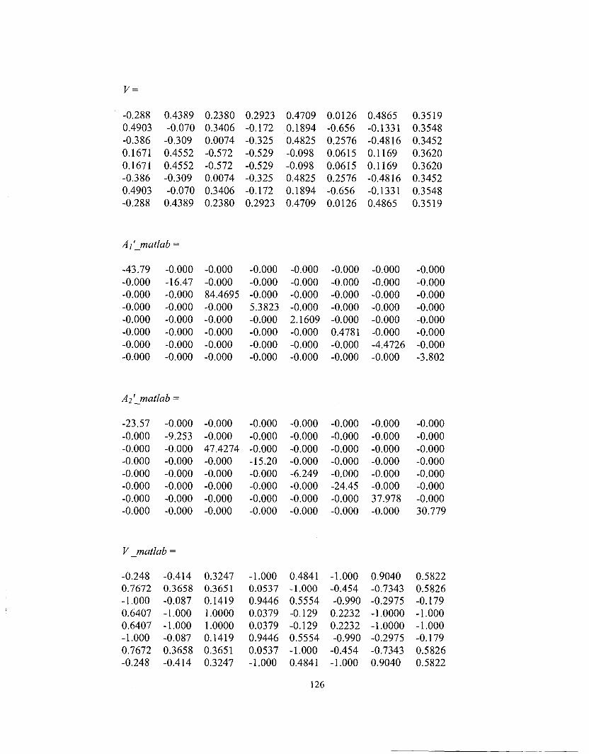
v= -0.288
0.4903
-0.386
0.1671
0.1671
-0.386
0.4903
-0.288
0.4389
-0.070
-0.309
0.4552
0.4552
-0.309 -0.070
0.4389
0.2380
0.3406
0.0074
-0.572
-0.572
0.0074
0.3406 0.2380
0.2923
-0.172
-0.325
-0.529
-0.529
-0.325
-0.172
0.2923
Ai'jnatlab =
-43.79
-0.000 -0.000
-0.000
-0.000
-0.000
-0.000
-0.000
-0.000
-16.47 -0.000
-0.000
-0.000
-0.000
-0.000 -0.000
-0.000
-0.000
84.4695
-0.000
-0.000
-0.000
-0.000 -0.000
-0.000
-0.000 -0.000
5.3823
-0.000
-0.000
-0.000 -0.000
AJjnatlab =
-23.57
-0.000
-0.000 -0.000
-0.000
-0.000
-0.000 -0.000
-0.000
-9.253
-0.000 -0.000
-0.000
-0.000 -0.000
-0.000
-0.000
-0.000
47.4274 -0.000
-0.000
-0.000
-0.000 -0.000
-0.000
-0.000
-0.000 -15.20
-0.000 -0.000
-0.000 -0.000
V matlab =
-0.248 0.7672
-1.000
0.6407 0.6407
-1.000
0.7672 -0.248
-0.414 0.3658
-0.087
-1.000 -1.000 -0.087
0.3658
-0.414
0.3247 0.3651
0.1419
1.0000
1.0000 0.1419 0.3651
0.3247
-1.000 0.0537
0.9446
0.0379
0.0379 0.9446
0.0537
-1.000
0.4709
0.1894
0.4825
-0.098
-0.098
0.4825
0.1894
0.4709
0.0126
-0.656
0.2576
0.0615
0.0615
0.2576
-0.656
0.0126
0.4865
-0.1331
-0.4816
0.1169
0.1169
-0.4816
-0.1331
0.4865
0.3519 0.3548
0.3452
0.3620
0.3620
0.3452
0.3548
0.3519
-0.000
-0.000
-0.000
-0.000
2.1609
-0.000
-0.000 -0.000
-0.000
-0.000 -0.000
-0.000
-0.000
0.4781
-0.000 -0.000
-0.000
-0.000
-0.000
-0.000
-0.000
-0.000
-4.4726
-0.000
-0.000
-0.000 -0.000
-0.000
-0.000
-0.000
-0.000 -3.802
0.000
0.000
0.000 0.000
6.249 0.000
0.000
0.000
-0.000
-0.000
-0.000 -0.000
-0.000
-24.45
-0.000 -0.000
-0.000
-0.000
-0.000 -0.000
-0.000
-0.000
37.978 -0.000
-0.000
-0.000
-0.000
-0.000
-0.000 -0.000
-0.000 30.779
0.4841 -1.000 0.5554
-0.129 -0.129 0.5554
-1.000 0.4841
-1.000 -0.454
-0.990
0.2232 0.2232
-0.990
-0.454
-1.000
0.9040
-0.7343 -0.2975
-1.0000
-1.0000 -0.2975
-0.7343 0.9040
0.5822 0.5826
-0.179
-1.000 -1.000
-0.179 0.5826
0.5822
126

140
120
100
80
60
40
20
0
-20
-40
-60
(a)
Proposed — + — Matlab-Cholesky --H
\
i i ! /. ' i i J
— _ j — J — i — + ' _
> i i - - * H — j — i —
0 j3 CD > C CD D)
i l l
80
60
40
20
0
-20
/in
(b)
— Proposed — +— Matlab-Cholesky
, _, _ _ _, _..
/
- / -
i i /
~-4-4-"Uq i V\
: :.. .__.)!.4 ._ i !\
.....±. L.y..:.....j
/ 4"V
2 4 6 Eigen value number
0 2 4 6 Eigen value number
Figure A-1.Comparison of the eigen-values of (a) matrix A 'i and A I'jnatlab (b) matrix
A'2and A 2'jnatlab
127
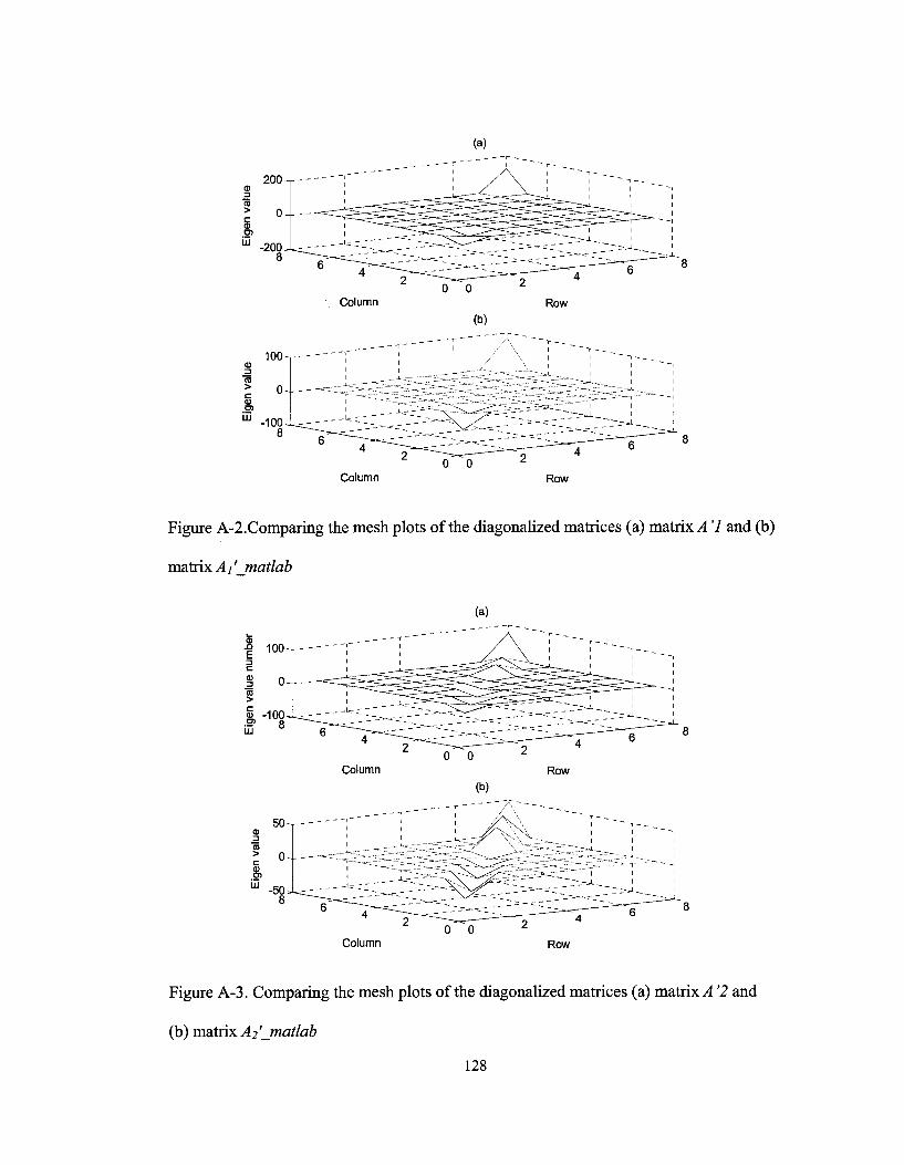
(a)
CD
,2 CD
> c d> u>
LU
200 - r - - -
0 0 Column Row
(b)
0 0 Column Row
Figure A-2.Comparing the mesh plots of the diagonalized matrices (a) matrix A '1 and (b)
matrix Ai 'jnatlab
(a)
0 0 Column Row
(b)
<B = 15 >
Eig
e
_ _ _ - - 1
5 0 - r - - - - - - r !
0 -
-50. 8
1 ' 1 _
' -- L ~ - - - - - " _ ~ :L~- -~
' _ - - a--__ " ~^-~i-^l" _ _"_"_---—-_-
0 0 Column Row
Figure A-3. Comparing the mesh plots of the diagonalized matrices (a) matrix A '2 and
(b) matrix Ajjnatlab
128