algorithmic and complexity aspects of simple coalitional...
TRANSCRIPT

Algorithmic and complexity aspects ofsimple coalitional games
Haris Aziz
A thesis submitted in partial fulfilment of therequirements for the degree of Doctor of Philosophy in
Computer Science
Department of Computer Science
University of Warwick


Contents
Acknowledgements . . . . . . . . . . . . . . . . . . . . . . . . . . . . . . . . . . . . . . . . . . . . . . XV
Declaration . . . . . . . . . . . . . . . . . . . . . . . . . . . . . . . . . . . . . . . . . . . . . . . . . . . . . XVII
Abbreviations and Symbols . . . . . . . . . . . . . . . . . . . . . . . . . . . . . . . . . . . . . . . XIX
Abstract . . . . . . . . . . . . . . . . . . . . . . . . . . . . . . . . . . . . . . . . . . . . . . . . . . . . . . . . 1
Biographical sketch . . . . . . . . . . . . . . . . . . . . . . . . . . . . . . . . . . . . . . . . . . . . . . 5
Part I Introduction
1 Introduction . . . . . . . . . . . . . . . . . . . . . . . . . . . . . . . . . . . . . . . . . . . . . . . . 91.1 Background . . . . . . . . . . . . . . . . . . . . . . . . . . . . . . . . . . . . . . . . . . . . . . 9
1.1.1 Game theory and computer science . . . . . . . . . . . . . . . . . . . . . 101.1.2 Algorithmic game theory & computational social choice
theory . . . . . . . . . . . . . . . . . . . . . . . . . . . . . . . . . . . . . . . . . . . . . 111.2 Thesis introduction . . . . . . . . . . . . . . . . . . . . . . . . . . . . . . . . . . . . . . . . 14
1.2.1 Overview . . . . . . . . . . . . . . . . . . . . . . . . . . . . . . . . . . . . . . . . . . 141.2.2 Simple games . . . . . . . . . . . . . . . . . . . . . . . . . . . . . . . . . . . . . . . 151.2.3 Approach of the thesis . . . . . . . . . . . . . . . . . . . . . . . . . . . . . . . . 16
1.3 Prerequisites . . . . . . . . . . . . . . . . . . . . . . . . . . . . . . . . . . . . . . . . . . . . . 171.4 Thesis outline . . . . . . . . . . . . . . . . . . . . . . . . . . . . . . . . . . . . . . . . . . . . 17
2 Preliminaries . . . . . . . . . . . . . . . . . . . . . . . . . . . . . . . . . . . . . . . . . . . . . . . . 232.1 Simple coalitional games . . . . . . . . . . . . . . . . . . . . . . . . . . . . . . . . . . . 232.2 Computational complexity . . . . . . . . . . . . . . . . . . . . . . . . . . . . . . . . . 27
VI Contents
Part II Computational voting
3 Complexity of comparison of influence of players in simple games . 333.1 Introduction . . . . . . . . . . . . . . . . . . . . . . . . . . . . . . . . . . . . . . . . . . . . . . 34
3.1.1 Overview and outline . . . . . . . . . . . . . . . . . . . . . . . . . . . . . . . . 343.2 Background . . . . . . . . . . . . . . . . . . . . . . . . . . . . . . . . . . . . . . . . . . . . . . 34
3.2.1 Definitions . . . . . . . . . . . . . . . . . . . . . . . . . . . . . . . . . . . . . . . . . 343.2.2 Desirability relation and linear games . . . . . . . . . . . . . . . . . . . 35
3.3 Compact representations . . . . . . . . . . . . . . . . . . . . . . . . . . . . . . . . . . . 363.4 Complexity of player types . . . . . . . . . . . . . . . . . . . . . . . . . . . . . . . . . 383.5 Complexity of desirability ordering . . . . . . . . . . . . . . . . . . . . . . . . . . 403.6 Power indices and Chow parameters . . . . . . . . . . . . . . . . . . . . . . . . . 463.7 Conclusion . . . . . . . . . . . . . . . . . . . . . . . . . . . . . . . . . . . . . . . . . . . . . . 51
4 Classification of computationally tractable weighted voting games . 534.1 Introduction . . . . . . . . . . . . . . . . . . . . . . . . . . . . . . . . . . . . . . . . . . . . . . 53
4.1.1 Motivation and outline . . . . . . . . . . . . . . . . . . . . . . . . . . . . . . . 534.2 Extreme cases . . . . . . . . . . . . . . . . . . . . . . . . . . . . . . . . . . . . . . . . . . . . 554.3 Bounded number of weight values . . . . . . . . . . . . . . . . . . . . . . . . . . . 56
4.3.1 All weights except one are equal . . . . . . . . . . . . . . . . . . . . . . . 564.3.2 Only two different weight values . . . . . . . . . . . . . . . . . . . . . . . 574.3.3 k weight values . . . . . . . . . . . . . . . . . . . . . . . . . . . . . . . . . . . . . 59
4.4 Distribution of weights . . . . . . . . . . . . . . . . . . . . . . . . . . . . . . . . . . . . 604.4.1 Geometric sequence of weights, and unbalanced weights . . . 604.4.2 Sequential weights . . . . . . . . . . . . . . . . . . . . . . . . . . . . . . . . . . . 63
4.5 Integer weights . . . . . . . . . . . . . . . . . . . . . . . . . . . . . . . . . . . . . . . . . . . 644.5.1 Moderate sized integer weights . . . . . . . . . . . . . . . . . . . . . . . . 644.5.2 Polynomial number of coefficients in the generating
function of the WVG . . . . . . . . . . . . . . . . . . . . . . . . . . . . . . . . . 644.6 Approximation approaches . . . . . . . . . . . . . . . . . . . . . . . . . . . . . . . . . 654.7 Open problems & conclusion . . . . . . . . . . . . . . . . . . . . . . . . . . . . . . . 66
5 Multiple weighted voting games . . . . . . . . . . . . . . . . . . . . . . . . . . . . . . . 695.1 Introduction . . . . . . . . . . . . . . . . . . . . . . . . . . . . . . . . . . . . . . . . . . . . . . 695.2 MWVGs . . . . . . . . . . . . . . . . . . . . . . . . . . . . . . . . . . . . . . . . . . . . . . . . 70
5.2.1 Structure . . . . . . . . . . . . . . . . . . . . . . . . . . . . . . . . . . . . . . . . . . . 705.2.2 Trade robustness . . . . . . . . . . . . . . . . . . . . . . . . . . . . . . . . . . . . 71
5.3 Properties of MWVGs . . . . . . . . . . . . . . . . . . . . . . . . . . . . . . . . . . . . . 71

Contents VII
5.4 Analysing MWVGs . . . . . . . . . . . . . . . . . . . . . . . . . . . . . . . . . . . . . . . 735.4.1 Generating functions for MWVGs . . . . . . . . . . . . . . . . . . . . . . 735.4.2 Analysis . . . . . . . . . . . . . . . . . . . . . . . . . . . . . . . . . . . . . . . . . . . 76
6 Efficient algorithm to design weighted voting games . . . . . . . . . . . . . 776.1 Introduction . . . . . . . . . . . . . . . . . . . . . . . . . . . . . . . . . . . . . . . . . . . . . . 78
6.1.1 Motivation . . . . . . . . . . . . . . . . . . . . . . . . . . . . . . . . . . . . . . . . . 786.1.2 Outline . . . . . . . . . . . . . . . . . . . . . . . . . . . . . . . . . . . . . . . . . . . . 78
6.2 Designing weighted voting games . . . . . . . . . . . . . . . . . . . . . . . . . . . 796.2.1 Outline and survey . . . . . . . . . . . . . . . . . . . . . . . . . . . . . . . . . . . 796.2.2 Algorithm to design weighted voting games . . . . . . . . . . . . . 806.2.3 Algorithmic and technical issues . . . . . . . . . . . . . . . . . . . . . . . 806.2.4 Performance and computational complexity . . . . . . . . . . . . . . 82
6.3 Designing egalitarian voting games . . . . . . . . . . . . . . . . . . . . . . . . . . 826.4 Multiple weighted voting games . . . . . . . . . . . . . . . . . . . . . . . . . . . . . 836.5 Conclusion & open problems . . . . . . . . . . . . . . . . . . . . . . . . . . . . . . . 84
7 EU: a case study . . . . . . . . . . . . . . . . . . . . . . . . . . . . . . . . . . . . . . . . . . . . . 877.1 Introduction . . . . . . . . . . . . . . . . . . . . . . . . . . . . . . . . . . . . . . . . . . . . . . 877.2 Appraisal of voting rules by power analysis . . . . . . . . . . . . . . . . . . . 907.3 The Penrose index approach . . . . . . . . . . . . . . . . . . . . . . . . . . . . . . . . 927.4 Analysis: voting power in EU27 . . . . . . . . . . . . . . . . . . . . . . . . . . . . . 947.5 Analysis: enlargement scenarios . . . . . . . . . . . . . . . . . . . . . . . . . . . . . 967.6 Conclusions . . . . . . . . . . . . . . . . . . . . . . . . . . . . . . . . . . . . . . . . . . . . . . 100
Part III Complexity of manipulation
8 Complexity of control in weighted voting games . . . . . . . . . . . . . . . . . 1078.1 Introduction . . . . . . . . . . . . . . . . . . . . . . . . . . . . . . . . . . . . . . . . . . . . . . 1088.2 Tolerance & amplitude: background . . . . . . . . . . . . . . . . . . . . . . . . . 109
8.2.1 Background . . . . . . . . . . . . . . . . . . . . . . . . . . . . . . . . . . . . . . . . 1098.2.2 Tolerance . . . . . . . . . . . . . . . . . . . . . . . . . . . . . . . . . . . . . . . . . . 1098.2.3 Amplitude . . . . . . . . . . . . . . . . . . . . . . . . . . . . . . . . . . . . . . . . . . 110
8.3 Tolerance & amplitude: some results . . . . . . . . . . . . . . . . . . . . . . . . . 1108.3.1 Complexity . . . . . . . . . . . . . . . . . . . . . . . . . . . . . . . . . . . . . . . . . 1108.3.2 Uniform and unanimity WVGs . . . . . . . . . . . . . . . . . . . . . . . . 111
8.4 Conclusion and future work . . . . . . . . . . . . . . . . . . . . . . . . . . . . . . . . 113
VIII Contents
9 False-name manipulations . . . . . . . . . . . . . . . . . . . . . . . . . . . . . . . . . . . . 1159.1 Introduction . . . . . . . . . . . . . . . . . . . . . . . . . . . . . . . . . . . . . . . . . . . . . . 1169.2 Related work . . . . . . . . . . . . . . . . . . . . . . . . . . . . . . . . . . . . . . . . . . . . . 1179.3 Splitting . . . . . . . . . . . . . . . . . . . . . . . . . . . . . . . . . . . . . . . . . . . . . . . . . 1179.4 Complexity of finding a beneficial split . . . . . . . . . . . . . . . . . . . . . . . 122
9.4.1 Pseudo-polynomial algorithm . . . . . . . . . . . . . . . . . . . . . . . . . 1249.5 Merging and annexation . . . . . . . . . . . . . . . . . . . . . . . . . . . . . . . . . . . 1259.6 Conclusions . . . . . . . . . . . . . . . . . . . . . . . . . . . . . . . . . . . . . . . . . . . . . . 132
10 Complexity of length, duality and bribery . . . . . . . . . . . . . . . . . . . . . . 13510.1 Introduction . . . . . . . . . . . . . . . . . . . . . . . . . . . . . . . . . . . . . . . . . . . . . . 136
10.1.1Background . . . . . . . . . . . . . . . . . . . . . . . . . . . . . . . . . . . . . . . . 13610.2Computing length of games . . . . . . . . . . . . . . . . . . . . . . . . . . . . . . . . 137
10.2.1Complexity of computing length . . . . . . . . . . . . . . . . . . . . . . . 13810.2.2Approximating the length of a MWVG . . . . . . . . . . . . . . . . . . 139
10.3Complexity of duality questions . . . . . . . . . . . . . . . . . . . . . . . . . . . . . 14210.4Bribery in WVGs . . . . . . . . . . . . . . . . . . . . . . . . . . . . . . . . . . . . . . . . . 145
10.4.1Under no information . . . . . . . . . . . . . . . . . . . . . . . . . . . . . . . . 14610.4.2Manipulation under full or partial information . . . . . . . . . . . . 148
10.5Conclusion . . . . . . . . . . . . . . . . . . . . . . . . . . . . . . . . . . . . . . . . . . . . . . 148
Part IV Resource Allocation & Networks
11 Cooperative game theory & simple games . . . . . . . . . . . . . . . . . . . . . . 15311.1 Introduction and background . . . . . . . . . . . . . . . . . . . . . . . . . . . . . . . 15411.2Related work . . . . . . . . . . . . . . . . . . . . . . . . . . . . . . . . . . . . . . . . . . . . . 15511.3Preliminaries . . . . . . . . . . . . . . . . . . . . . . . . . . . . . . . . . . . . . . . . . . . . . 15511.4Cooperative game theory solutions . . . . . . . . . . . . . . . . . . . . . . . . . . . 158
11.4.1Introduction . . . . . . . . . . . . . . . . . . . . . . . . . . . . . . . . . . . . . . . . 15811.4.2Desirability relation and cooperative game solutions . . . . . . 16311.4.3Generalized problems . . . . . . . . . . . . . . . . . . . . . . . . . . . . . . . . 163
11.5Core . . . . . . . . . . . . . . . . . . . . . . . . . . . . . . . . . . . . . . . . . . . . . . . . . . . . 16411.6Core stability . . . . . . . . . . . . . . . . . . . . . . . . . . . . . . . . . . . . . . . . . . . . . 16511.7Least core . . . . . . . . . . . . . . . . . . . . . . . . . . . . . . . . . . . . . . . . . . . . . . . 16711.8Nucleolus . . . . . . . . . . . . . . . . . . . . . . . . . . . . . . . . . . . . . . . . . . . . . . . 17311.9Kernel and bargaining set . . . . . . . . . . . . . . . . . . . . . . . . . . . . . . . . . . 177
11.9.1Wolsey’s theorem . . . . . . . . . . . . . . . . . . . . . . . . . . . . . . . . . . . 17911.10Cost of stability . . . . . . . . . . . . . . . . . . . . . . . . . . . . . . . . . . . . . . . . . . 18011.11Conclusion and open problems . . . . . . . . . . . . . . . . . . . . . . . . . . . . . . 183

Contents IX
12 Power indices of spanning connectivity games . . . . . . . . . . . . . . . . . . . 18512.1 Introduction . . . . . . . . . . . . . . . . . . . . . . . . . . . . . . . . . . . . . . . . . . . . . . 18512.2Related work . . . . . . . . . . . . . . . . . . . . . . . . . . . . . . . . . . . . . . . . . . . . . 18712.3Preliminaries . . . . . . . . . . . . . . . . . . . . . . . . . . . . . . . . . . . . . . . . . . . . . 187
12.3.1Graph theory . . . . . . . . . . . . . . . . . . . . . . . . . . . . . . . . . . . . . . . 18712.3.2Spanning connectivity game . . . . . . . . . . . . . . . . . . . . . . . . . . . 188
12.4Complexity of computing power indices . . . . . . . . . . . . . . . . . . . . . . 18812.5Polynomial time cases . . . . . . . . . . . . . . . . . . . . . . . . . . . . . . . . . . . . . 19112.6Other power indices . . . . . . . . . . . . . . . . . . . . . . . . . . . . . . . . . . . . . . . 19712.7Conclusion . . . . . . . . . . . . . . . . . . . . . . . . . . . . . . . . . . . . . . . . . . . . . . 197
13 Nucleolus of spanning connectivity games . . . . . . . . . . . . . . . . . . . . . . 19913.1 Introduction . . . . . . . . . . . . . . . . . . . . . . . . . . . . . . . . . . . . . . . . . . . . . . 20013.2Related work . . . . . . . . . . . . . . . . . . . . . . . . . . . . . . . . . . . . . . . . . . . . . 20113.3Least core of SCGs . . . . . . . . . . . . . . . . . . . . . . . . . . . . . . . . . . . . . . . 20113.4Cut-rate . . . . . . . . . . . . . . . . . . . . . . . . . . . . . . . . . . . . . . . . . . . . . . . . . 20313.5Prime Partition . . . . . . . . . . . . . . . . . . . . . . . . . . . . . . . . . . . . . . . . . . . 216
13.5.1Construction of the prime-partition . . . . . . . . . . . . . . . . . . . . . 21813.5.2The output of Algorithm 12 is the prime partition . . . . . . . . . 220
13.6Parent-child relation . . . . . . . . . . . . . . . . . . . . . . . . . . . . . . . . . . . . . . . 22413.7Nucleolus . . . . . . . . . . . . . . . . . . . . . . . . . . . . . . . . . . . . . . . . . . . . . . . 23313.8Wiretap game . . . . . . . . . . . . . . . . . . . . . . . . . . . . . . . . . . . . . . . . . . . . 23513.9Conclusion . . . . . . . . . . . . . . . . . . . . . . . . . . . . . . . . . . . . . . . . . . . . . . 237
Part V Conclusion
14 Concluding remarks . . . . . . . . . . . . . . . . . . . . . . . . . . . . . . . . . . . . . . . . . 241
Part VI Appendices
A MWVG Program . . . . . . . . . . . . . . . . . . . . . . . . . . . . . . . . . . . . . . . . . . . . 247
Part VII Backmatter
References . . . . . . . . . . . . . . . . . . . . . . . . . . . . . . . . . . . . . . . . . . . . . . . . . . . . . . 255
Index . . . . . . . . . . . . . . . . . . . . . . . . . . . . . . . . . . . . . . . . . . . . . . . . . . . . . . . . . . 267


List of Tables
3.1 Complexity of comparing players . . . . . . . . . . . . . . . . . . . . . . . . . . . 52
4.1 Complexity of WVG classes . . . . . . . . . . . . . . . . . . . . . . . . . . . . . . . 67
9.1 Complexity of false name manipulations in WVGs . . . . . . . . . . . . 1319.2 Bounds of false-name manipulations in WVGs . . . . . . . . . . . . . . . . 132
10.1 Complexity of dualization, length and bribery . . . . . . . . . . . . . . . . . 148
11.1 Cooperative game solutions and desirability relation in simplegames . . . . . . . . . . . . . . . . . . . . . . . . . . . . . . . . . . . . . . . . . . . . . . . . . . 163
11.2 Complexity of cooperative game solutions in simple games . . . . . 184
12.1 Complexity of SCGs . . . . . . . . . . . . . . . . . . . . . . . . . . . . . . . . . . . . . . 198
13.1 Spanning connectivity game and the wiretap game . . . . . . . . . . . . . 237


List of Figures
1.1 Decision making models . . . . . . . . . . . . . . . . . . . . . . . . . . . . . . . . . . 13
6.1 Mathematica program to design WVGs . . . . . . . . . . . . . . . . . . . . . . 85
7.1 Voting Power Analysis of the EU27 . . . . . . . . . . . . . . . . . . . . . . . . . 957.2 Citizen Indirect Power Indices Under All Scenarios: Reform Treaty 987.3 Citizen Indirect Power Indices Under All Scenarios: Jagiellonian
Compromise . . . . . . . . . . . . . . . . . . . . . . . . . . . . . . . . . . . . . . . . . . . . . 997.4 Relative Citizen Power: Large Countries . . . . . . . . . . . . . . . . . . . . . 1017.5 Relative Citizen Voting Power: Middle-sized Countries . . . . . . . . . 1027.6 Relative Citizen Voting Power: Small Countries . . . . . . . . . . . . . . . 103
9.1 Splitting of player i into i′ and i′′ . . . . . . . . . . . . . . . . . . . . . . . . . . . . 119
11.1 Relations of cooperative games I . . . . . . . . . . . . . . . . . . . . . . . . . . . . 15711.2 Relations of cooperative games II . . . . . . . . . . . . . . . . . . . . . . . . . . . 15711.3 Relations of cooperative game solutions . . . . . . . . . . . . . . . . . . . . . . 162
12.1 Multigraph and its underlying graph . . . . . . . . . . . . . . . . . . . . . . . . . 195
13.1 Prime Partition . . . . . . . . . . . . . . . . . . . . . . . . . . . . . . . . . . . . . . . . . . 232


Acknowledgements
Gratitude is the memory of the heart.
- French Proverb
I am grateful to Almighty for being so kind to me. I am thankful to my wifeSana for being such a wonderful partner in every way. I thank my parents fortheir love and faith in me and to my siblings Kashif, Saba for supporting me. Ialso want to express my gratitude to both of my supervisors Prof. Mike Patersonand Prof. Dennis Leech for their assistance and patient guidance throughout theproject. A PhD thesis does not only require academic support and, in this context,I am especially indebted to Mike who, despite his many commitments, alwaysfound time to discuss any issue.
I acknowledge the contribution of the Warwick ‘Algorithms and Complexity’research group towards funding my research. It has been a pleasure to work withOded Lachish and Rahul Savani. Prof. Artur Czumaj has also been a very sup-portive figure in the department. I want to thank the following people, projectsand organizations for facilitating some useful research visits: International Foun-dation for Autonomous Agents and Multiagent Systems (IFAAMAS), COST Ac-tion IC0602, British Colloquium for Theoretical Computer Science, Prof. AlexisTsoukias and Dr. Ulle Endriss.
Thanks are also due to Elias, James and Jendrik for the numerous tennis hitswe had. I would also like to express thanks to my teachers, especially Prof. ZaeemJafri, Prof. Wasiq Hussain, Prof. Ismet Beg, Prof. Peter Jeavons and last, but

XVI Acknowledgements
certainly not the least, Prof. Sarmad Abbasi who got me hooked to theoreticalcomputer science.
Kenilworth, Haris Aziz
July 2009

Declaration
This thesis contains published work and work which has been co-authored. Thefollowing chapters are based on various publications respectively: Chapter 3 [10],Chapter 4 [16], Chapter 5 [15], Chapter 6 [19], Chapter 7 [137], Chapter 8 [17],Chapter 9, [18], Chapter 10 [11], Chapter 12 [13] and Chapter 13 [14]. The re-search was led and conducted by me with support and feedback from my su-pervisors. The work on spanning connectivity games [13, 14] involved closelyworking with Rahul Savani and Oded Lachich.

Abbreviations and Symbols
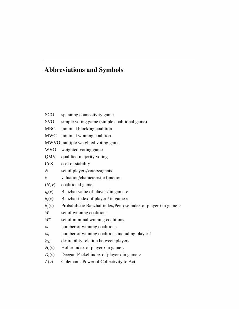
SCG spanning connectivity gameSVG simple voting game (simple coalitional game)MBC minimal blocking coalitionMWC minimal winning coalitionMWVG multiple weighted voting gameWVG weighted voting gameQMV qualified majority votingCoS cost of stabilityN set of players/voters/agentsv valuation/characteristic function(N, v) coalitional gameηi(v) Banzhaf value of player i in game v
βi(v) Banzhaf index of player i in game v
β′
i(v) Probabilistic Banzhaf index/Penrose index of player i in game v
W set of winning coalitionsWm set of minimal winning coalitionsω number of winning coalitionsωi number of winning coalitions including player i
�D desirability relation between playersHi(v) Holler index of player i in game v
Di(v) Deegan-Packel index of player i in game v
A(v) Coleman’s Power of Collectivity to Act

XX Abbreviations and Symbols
τ[q; w1, . . . ,wn] tolerance of a weighted voting gameµ[q; w1, . . . ,wn] amplitude of a weighted voting game((N \ S ) ∪ {&S }, v&S ) (N, v) where players in in coalition S have mergede(x, S ) excess of coalition S according to payoff x
−εi(x, v) ith distinct worst excess for payoff x and game v
−ε1(v) worst excess for a least core payoff of game v
δi(x, v) 1 − εi(x, v)δ1(v) least core payoff of a coalition with the worst excessAi
x(v) set of coalitions that get excess −εi(x, v)sv
i j(x) maximum surplus of player i over player j with respect to x
l(v) length of coalitional game (N, v)I∗(v) set of preimputations of game v
I(v) set of imputations of game v
Ni number of winning coalitions of cardinality i
Gx weighted graph with edge e having weight x(e)E(α) edge partition for imputation αCG(E′) number of connected components in the graph G \ E′
crG(E′) cut-rate of edge set E′ in graph G
opt maxE′⊆E cr(E′)P prime-partition of a graphO parent-child relation in a graph

To late Professor Zaeem Jafri to whom I owe a lot


Abstract
Thesis Title: Algorithmic & complexity aspects of simple coalitional gamesBy: Haris AzizPlace: University of WarwickYear: 2009Supervisor: Prof. Mike PatersonCo-supervisor: Prof. Dennis LeechThesis committee: Prof. Paul Goldberg, Prof. Artur Czumaj and Prof. Alex Tiskin.
Simple coalitional games are a fundamental class of cooperative games andvoting games which are used to model coalition formation, resource allocationand decision making in computer science, artificial intelligence and multiagentsystems. Although simple coalitional games are well studied in the domain ofgame theory and social choice, their algorithmic and computational complexityaspects have received less attention till recently. The computational aspects ofsimple coalitional games are of increased importance as these games are usedby computer scientists to model distributed settings. This thesis fits in the widersetting of the interplay between economics and computer science which has ledto the development of algorithmic game theory and computational social choice.A unified view of the computational aspects of simple coalitional games is pre-sented here for the first time. Certain complexity results also apply to other coali-tional games such as skill games and matching games. The following issues aregiven special consideration: influence of players, limit and complexity of ma-

2 Abstract
nipulations in the coalitional games and complexity of resource allocation onnetworks. The complexity of comparison of influence between players in simplegames is characterized. The simple games considered are represented by win-ning coalitions, minimal winning coalitions, weighted voting games or multi-ple weighted voting games. A comprehensive classification of weighted votinggames which can be solved in polynomial time is presented. An efficient algo-rithm which uses generating functions and interpolation to compute an integerweight vector for target power indices is proposed. Voting theory, especially thePenrose Square Root Law, is used to investigate the fairness of a real life vot-ing model. Computational complexity of manipulation in social choice proto-cols can determine whether manipulation is computationally feasible or not. Thecomputational complexity and bounds of manipulation are considered from var-ious angles including control, false-name manipulation and bribery. Moreover,the computational complexity of computing various cooperative game solutionsof simple games in different representations is studied. Certain structural resultsregarding least core payoffs extend to the general monotone cooperative game.The thesis also studies a coalitional game called the spanning connectivity game.It is proved that whereas computing the Banzhaf values and Shapley-Shubik in-dices of such games is #P-complete, there is a polynomial time combinatorialalgorithm to compute the nucleolus. The results have interesting significance foroptimal strategies for the wiretapping game which is a noncooperative game de-fined on a network.
Keywords: Cooperative games, game theory, algorithms and complexity, multia-gent systems, network connectivity, network security, power indices, Shapley-Shubik index, Banzhaf index, Chow parameters, computational social choice,simple voting games, weighted voting games, nucleolus, least-core, cost of sta-bility, resource allocation, preference aggregation, Nash equilibria, kernel, bar-gaining set, stable set, linear programming.

Abstract 3
Association for Computing Machinery (ACM) Categories:F.2 [Theory of Computation]: Analysis of Algorithms and Problem ComplexityI.2.11 [Distributed Artificial Intelligence]: Multiagent SystemsJ.4 [Computer Applications]: Social and Behavioral Sciences - Economics
Mathematics Subject Classification (MSC): 91A12, 91A43, 91A46, 05C40,68Q15, 68Q17, 68W40


Biographical sketch
Haris Aziz received a BSc(Honours) in Computer Science from Lahore Univer-
sity of Management Sciences in 2003 and an MSc in Mathematics and Founda-tions of Computer Science from the University of Oxford in 2005. He expects toreceive a PhD in Computer Science from the University of Warwick in 2009. FromAugust 2009, he is a European Science Foundation (ESF) postdoctoral researcherin a Europe-wide collaborative research project on “Computational Foundationsof Social Choice” and is based at the Ludwig-Maximilians-University Munich.


Part I
Introduction


1
Introduction
There are no disciplines, nor branches of knowledge - or rather of re-
search; there are only problems and the need to solve them.
- Karl Popper, “Realism and the Aim of Science” from the ‘Postscript to
the Logic of Scientific Discovery (1983)’
Many applications in computer science involve issues and problems that
decision theorists have addressed for years, issues of preference, utility,
conflict and cooperation, allocation, incentives, consensus, social choice,
and measurement. A similar phenomenon is apparent more generally at
the interface between computer science and the social sciences.
- Fred S. Roberts [186]
Abstract In this chapter, the general background and an outline of the thesis ispresented.
1.1 Background
I do think there are some very worthwhile and interesting analogies be-
tween complexity issues in computer science and in economics. For exam-
ple, economics traditionally assumes that the agents within an economy
have universal computing power . . . Computer scientists deny that an al-
gorithm can have infinite computing power.
- Richard Karp [117]
10 1 Introduction
1.1.1 Game theory and computer science
Decision theory, game theory, and social choice theory are well-established fieldswhich involve modeling the interaction between agents. Social choice concernsthe aggregation of different self-interested agents’ preferences. It encapsulatesvarious important processes such as voting, markets and auctions where dis-tributed agents want to make joint decisions. Game theory is the study of the con-flict, cooperation and outcomes of interactions amongst multiple agents. Mech-anism design is the design of games in such a way that individual players moti-vated by self-interest satisfy the desired goals of the designer. The desired goalcould be individual rationality, budget balance, maximize total social welfare orto elicit truthful behaviour. Mechanism design1 has been considered as the inverseof game theory [167].
Game theory, social choice theory and mechanism design, which were tradi-tionally in the domain of economics and decision theory, are increasingly be-ing used by computer scientists as tools to analyse distributed settings. Withthe growth of the internet, these fields provide an appropriate framework tomodel agents in the network [81]. Moreover, economics models and paradigmsare being examined in the new light of the inherent computational complex-ity of the relevant problems. Nisan [158] elaborates on the two-way flow ofideas between economics and computer science. Not only are algorithmic chal-lenges taking into account social choice and economic paradigms, but variouseconomic interactions such as voting, coalition formation and resource alloca-tion are requiring deeper algorithmic study. Similarly, Tennenholtz discussesthe trend of the interaction between computer science/artificial intelligence andgame theory/economics [203]. The same trend has also been pointed out else-where [47, 138]. In an earlier paper, Urken [208] shows that voting theory isessential in distributed decision making and network reliability. Rosenschein andProcaccia [187] observe how social choice theory is fundamental to analysingand designing multiagent systems and why algorithmic and complexity exam-
1 Hurwicz, Maskin and Myerson received the 2007 Nobel Memorial Prize in Economic Sciences “forhaving laid the foundations of mechanism design theory”.

1.1 Background 11
ination is critical in social choice protocols. Wellman [215] points out that aneconomic approach is fundamental for resource allocation, rationality abstrac-tion and decentralized control. The interface between game theory and computerscience is further highlighted by Al Roth [188]. A computational perspective ongame theoretic models is fundamental to new developments in computer science,game theory and multiagent systems. A combined game theoretic and algorith-mic approach is even more important because of the convergence of social andtechnological networks [119].
1.1.2 Algorithmic game theory & computational social choice theory
As the ice separating Game Theory from Theoretical Computer Science
is melting, some of the fundamental results in Game Theory come under
increased complexity-theoretic scrutiny.
- Fabrikant, Papadimitriou and Talwar [72]
Mathematical economics has been around for decades. Although major de-velopments have been made in presenting predictive theories and sound solutionconcepts, the treatment has mostly been non-algorithmic. It is essential that thesolutions are not only axiomatically desirable and predictive but also computa-tionally tractable. A computational perspective tries to answer various questionswhich are not tackled in classical economics and game theory: how efficiently cana model be represented? What is the complexity of computing a certain solution?How much memory will be required? Is this the best we can do? If computation isdone on a network, how much communication is needed? Work on social choiceand mechanism design has ignored such computational concerns till recent times.Therefore, there is a pressing need to revisit concepts in mathematical economicsand game theory from a computational point of view. Economic systems workbecause all the participants try to selfishly optimize their own objectives. Often,this optimization is intractable because of the computational complexity of theoptimization or lack of information. In that case, computational considerationsare paramount.

12 1 Introduction
The computational complexity of computing social choice functions, rank-ings, various concepts of equilibria, cooperative game solution concepts, tour-nament solutions, power indices, optimal or dominant strategies helps us under-stand what can be computed efficiently and what requires alternative approacheslike approximation algorithms, randomized algorithms, parameterized complex-ity and heuristics. As we will see in the thesis, notions of computational in-tractability such as NP-hardness are useful barriers to manipulative behaviour insocial choice settings. These have parallels with cryptographic protocols wherethe lack of efficient algorithms to factorize numbers helps avoid harmful attacks.The approach is that whereas social choice protocols may not be strategy-proof,it is desirable to design them in a way so that they are strategy-resistant. Anotheraspect of decision theory and game theory, which requires computer science con-siderations, is compact representation. As various models in game theory are im-plemented in computer science applications, there is a need to find more compactrepresentations of games and ways of encoding information.
The interaction of social choice and game theory with computer science in-cludes bounded rationality, computation of Nash equilibrium, algorithmic mech-anism design, price of anarchy, learning in games and efficient representationsof games, Byzantine agreement and implementing mediators. Interestingly, thisintimate encounter between computer science and game theory dates back to vonNeumann who made ground-breaking contributions to both fields. Game theory,decision theory and computer science have had more fruitful developments in re-cent years [186]. In the general realm of decision theory, decision making modelshave been classified (see Figure 1.1 [127]):
Among these models, simple coalitional games belong to the domains of bothdecision theory and cooperative game theory. Compared to non-cooperative gametheory in which individual agents are analysed, cooperative game theory is con-cerned with analyzing which coalitions will form and how the coalitions shoulddivide the payoff among their members. In recent years, there has been signif-icant work in the theoretical computer science community on non-cooperativegame theory. Whereas the computational complexity aspects of non-cooperative

1.1 Background 13
Objectives
One
Two or more
One
Operations Research
Multicrtieria Decision
Players
Cooperative
Games Noncooperative
Games
Two or more
Fig. 1.1. Decision making models
game theory, such as computing Nash equilibria, have started to be examinedby theoretical computer scientists with greater intensity [168], there is a needto revisit cooperative game theory with a computational lens. Yoav Shoham andLeyton-Brown in the introduction of [195] have observed this need. Interestingly,in Chapter 13, we will find a case where cooperative game theory is used to solvea problem in non-cooperative game theory. In modeling decision making by oneplayer, many problems turn out to be combinatorial optimization problems. How-ever, when multiple players are involved in decision making, cooperative gametheory [58] has a role to play in maximizing objectives of players and resourceallocation. The computational complexity of computing solutions and decidingwhether a payoff is in a class of solutions is an important consideration. This
14 1 Introduction
consideration also ties in with bounded rationality which argues that a decisionmaker can not spend an unbounded amount of resources.
Voting models are not necessarily restricted to analysing political scenarios.Similar interaction happens in multiagent systems and virtual environments. Con-sensus and voting problems arise in meta-search, collaborative filtering and dis-tributed computing [128]. Shoham in a recent survey [194] observes that the in-teraction between computer science and game theory has currently been focusedon six areas among which the first three are: 1) compact game representations,2) complexity of, and algorithms for, computing solution concepts and 3) algo-rithmic aspects of mechanism design. In many respects, these current issues areaddressed from the point of view of simple coalitional games.
1.2 Thesis introduction
...few structures arise in more contexts and lend themselves to more di-
verse interpretations than do simple games
- Taylor and Zwicker [202]
1.2.1 Overview
This thesis examines the computational and algorithmic aspects of simple votinggames or cooperative simple games which are not only an important class of co-operative games but also a widely used voting model. The mathematical modelof simple games is generic enough to model various scenarios. The research fo-cusses on algorithms and the complexity of analysing the influence of players ingame theoretic situations. This study of influence is significant in fields as diverseas percolation theory, reliability theory, political science and game theory [116].The thesis also examines susceptibility of simple games, especially weighted vot-ing games, to various kinds of manipulations. Manipulation is an urgent issue inmultiagent systems and it has been observed that not only do coalitional votinggames model various multiagent scenarios well, but computational complexity isseen as a useful barrier against manipulation.

1.2 Thesis introduction 15
A comprehensive investigation of the influence of players in simple gamespromises to be a useful contribution to the literature considering that the notionhas not been explored much in the works [213] and [202]. Taylor and Zwickernote in the preface of [202] that the cardinal notions of power have not been men-tioned in their book. Interestingly, such notions of power are now being exploredmuch more in communities as diverse as reliability theory, political science andmulti-agent systems. Voting power is also used in joint stock companies whereeach shareholder gets votes in proportion to the ownership of a stock [94]. An al-gorithms and complexity study of the influence of players is particularly relevantwith the increase of large scale multi-agent systems. Moreover, in the manuscripton ‘Challenges for Theoretical Computer Science’ by Johnson [115], the fol-lowing challenges are highlighted: preventing strategic voting, computing powerindices, continuing exploring the impact of bounded rationality and developing atheory of algorithmic mechanism design.
1.2.2 Simple games
...we will arrive at an extensive class of games, to be called simple. It will
be seen that a study of this class yields a body of information which is of
value for a deep understanding of the general theory...
- von Neumann and O. Morgenstern [213]
Simple games (which are yes/no decision games) were introduced in the clas-sical work of von Neumann and Morgenstern [213]. Von Neumann and Mor-genstern point out that a study of simple games makes it possible to get an un-derstanding of more general but harder to study zero-sum n-person games. Sim-ple games have a rich mathematical history with contributions from game theo-rists, computer scientists, electrical engineers and combinatorialists. The historyof simple games could even be stretched back to the famous Dedekind prob-
lem [120]. In 1897, Dedekind asked for the number d(n) of free distributive lat-tices on n elements. This problem is equivalent to the number of simple games onn players. The Dedekind problem has been well studied. The function d(n) growsrapidly and d(n) is only known for very small n. Various algorithms have been

16 1 Introduction
proposed for efficient computation of d(n) [85]. Simple games also have connec-tions with Sperner theory [71]. As in the case of Taylor and Zwicker [202], wewill discuss simple games in a voting-theoretic context. This is convenient bothfrom an intuition and notation point of view.
Simple games and weighted voting games (which are a sub-class of simplegames) are known in different literatures and communities by different names.There is considerable work on these models in threshold logic [216, 109, 154]and also in game theory (see [202] for a detailed literature references).
Weighted voting games (WVGs) are mathematical models which are used toanalyze voting bodies in which the voters have different number of votes. InWVGs, each voter is assigned a non-negative weight and makes a vote in favourof or against a decision. The decision is made if and only if the total weightof those voting in favour of the decision is greater than or equal to some fixedquota. Since the weights of the players do not always exactly reflect how criticala player is in decision making, voting power attempts to measure the ability of aplayer in a WVG to determine the outcome of the vote. WVGs are also encoun-tered in threshold logic, reliability theory, neuroscience and logical computingdevices ([202], [208]). Parhami [171] points out that voting has a long historyin reliability systems dating back to von Neumann [212]. For reliability systems,the weights of a WVG can represent the significance of the components whereasthe quota can represent the threshold for the overall system to fail. Systems ofthis type are used in various areas such as target and pattern recognition, safetymonitoring and human organization systems. WVGs have been applied in variouspolitical and economic organizations ([1]).
1.2.3 Approach of the thesis
...every definite mathematical problem must necessarily be susceptible of
an exact settlement, either in the form of an actual answer to the question
asked, or by the proof of the impossibility of its solution
- David Hilbert (1900 lecture)

1.4 Thesis outline 17
The approach of the thesis is algorithmic. For many problems in cooperativegame theory and social choice theory, there are mathematical results such as theexistence or non-existence of properties. However, there is a need for an algorith-mic study of these topics so that efficient constructive methods can be devisedto test different properties of games. For various computational problems asso-ciated with simple coalitional games, polynomial time exact algorithms, pseudo-polynomial algorithms, approximation algorithms and parameterized algorithmsare presented. In other cases, a proof is provided that the problem is, for instance,NP-hard or #P-complete.
1.3 Prerequisites
The thesis presupposes familiarity with combinatorial optimization and computa-tional complexity. For readers unfamiliar with these areas, the following excellentbook is recommended: [169]. In Section 2.2, non-technical definitions of funda-mental complexity classes are given. One may also refer to Section 1.2 of [173]which outlines some basics of discrete optimization.
1.4 Thesis outline
The thesis is one of the first unified treatments of simple coalitional games froma computational perspective.
Chapter 3: In this chapter, the complexity of comparison of influence be-tween players in simple games is characterized. The chapter is based on [10].The influence of players is gauged from the viewpoint of basic player types, de-sirability relations and classical power indices such as the Shapley-Shubik index,Banzhaf index, Holler index, Deegan-Packel index and Chow parameters. Amongother results, it is shown that for a simple game represented by its set of minimalwinning coalitions Wm, although it is easy to verify whether a player has votingpower zero or one, computing the Banzhaf value of the player is #P-complete.Moreover, it is proved that for multiple weighted voting games, it is NP-hard to

18 1 Introduction
verify whether the game is linear or not. For a simple game on n players andrepresented by Wm, a O(n.|Wm| + n2 log n) algorithm is presented which returns‘no’ if the game is non-linear and returns the strict desirability ordering other-wise. It is also shown that, for any reasonable representation of a simple game,a polynomial time algorithm to compute the Shapley-Shubik indices implies apolynomial time algorithm to compute the Banzhaf indices. As a corollary, wesettle the complexity of computing the Shapley value of a number of networkgames. The complexity of transforming simple games into compact representa-tions is also examined.
Chapter 4: It is well known that computing Banzhaf indices in a weightedvoting game is #P-complete. We give a comprehensive classification of thoseweighted voting games which can be solved in polynomial time. Among otherresults, we provide a polynomial (O(k(n
k )k)) algorithm to compute the Banzhaf in-dices in weighted voting games in which the number of weight values is boundedby k. The chapter is based on [16].
Chapter 5: We study the mathematical and computational aspects of multipleweighted voting games which are an extension of weighted voting games. Weanalyse the structure of multiple weighted voting games and some of their com-binatorial properties especially with respect to dictatorship, veto power, dummyplayers and Banzhaf indices. An illustrative Mathematica program to computevoting power properties of multiple weighted voting games is also provided. Thechapter is based on the following publication: [15].
Chapter 6: The calculation of voting powers of players in a weighted votinggame has been extensively researched in the last few years. However, the inverseproblem of designing a weighted voting game with a desirable distribution ofpower has received less attention. We present an efficient algorithm which usesgenerating functions and interpolation to compute an integer weight vector fortarget Banzhaf power indices. This algorithm has better performance than anyother known to us. It can also be used to design egalitarian two-tier weightedvoting games and a representative weighted voting game for a multiple weighted

1.4 Thesis outline 19
voting game. The results in this chapter are based on paper [19] written with mysupervisors.
Chapter 7: This chapter is based on a paper [137] jointly written with DennisLeech. We tested a heuristic on the real life case-study of the EU constitution.The Double Majority rule in the Reform Treaty agreed in Rome in September2004 is claimed to be simpler, more transparent and more democratic than theexisting rule. We use voting power analysis to examine these questions againstthe democratic ideal that the votes of all citizens in whatever member countryshould be of equal value. We also consider possible future enlargements involvingcandidate countries and then a number of hypothetical future enlargements. Wefind the Double Majority rule fails to measure up to the democratic ideal in allcases. We find the Jagiellonian compromise to be very close to this ideal.
Chapter 8: An important aspect of mechanism design in social choice pro-tocols and multiagent systems is to discourage insincere behaviour. Manipu-lative behaviour has received increased attention since the famous Gibbard-Satterthwaite theorem. We examine the computational complexity of manipula-tion in weighted voting games, which are ubiquitous mathematical models used ineconomics, political science, neuroscience, threshold logic, reliability theory anddistributed systems. It is a natural question to check how changes in a weightedvoting game may affect the overall game. The tolerance and amplitude of aweighted voting game signify the possible variations in a weighted voting gamewhich still keep the game unchanged. We characterize the complexity of comput-ing the tolerance and amplitude of weighted voting games. Tighter bounds andresults for the tolerance and amplitude of key weighted voting games are alsoprovided. Results from this chapter were published in [17].
Chapter 9: We examine the computational complexity of false-name manip-ulation in weighted voting games. This includes checking how much the Banzhafindex of a player increases or decreases if it splits up into sub-players. A pseudo-polynomial algorithm to find the optimal split is also provided. In the chapter, wealso examine the cases where a player annexes other players or merges with themto increase their Banzhaf index or Shapley-Shubik index payoff. We characterize
20 1 Introduction
the computational complexity of such manipulations as well as providing limits tothe manipulation. The Annexation Non-monotonicity paradox is also discoveredin the case of the Banzhaf index. The results give insight into coalition formationand manipulation. The chapter is based on a paper [18] co-authored with MikePaterson.
Chapter 10: This chapter is based on the following paper: [11]. Length andwidth are important characteristics of coalitional voting games which indicatethe efficiency of making a decision. Duality theory also plays an important rolein artificial intelligence. In this chapter, the complexity of problems concerningthe length, width and minimal winning coalitions of simple games is analysed.The complexity of questions related to duality of simple games such as DUAL,DUALIZE and SELF-DUAL is also examined. Since susceptibility to manipula-tion is a major issue in multiagent systems, it is observed that the results obtainedhave direct bearing on susceptibility to optimal bribery in simple games.
Chapter 11: In this chapter, cooperative games and cooperative game solu-tions are introduced. The trend of using computational tractability as a criterionfor cooperative game solutions is both recent and prevalent in the mathematicsof operations research and theoretical computer science. In this chapter, the com-putational aspects of various cooperative game solutions in simple games areexamined. Questions considered include the following: 1) for solution set X andsimple game v, is X of v empty or not, 2) compute an element in X of v and 3)verify if a payoff is in X of v. Some representations taken into account are simplegames represented by W, Wm, weighted voting games and multiple weighted vot-ing games. The cooperative solutions considered are the core, ε-core, least-core,nucleolus, prekernel, kernel, bargaining set and stable sets. The complexity ofchecking the stability of the core of simple games is also examined. A theoremfrom the paper “The nucleolus and kernel for simple games or special valid in-equalities for 0 − 1 linear integer programs” by Wolsey is corrected. Finally, therelation between cost of stability and the least core is examined. A natural anddesirable solution called the super-nucleolus is also proposed.

1.4 Thesis outline 21
Chapters 12 and 13 concern spanning connectivity games (SCGs). They arebased on joint work with Oded Lachish, Mike Paterson and Rahul Savani.
Chapter 12:We examine the computational complexity of computing the voting power
indices of edges in the SCG. It is shown that computing Banzhaf values is #P-complete and computing Shapley-Shubik indices or values is NP-hard for SCGs.Interestingly, Holler indices and Deegan-Packel indices can be computed in poly-nomial time. Among other results, it is proved that Banzhaf indices can be com-puted in polynomial time for graphs with bounded tree-width. Results from thischapter were published in [13].
Chapter 13: We consider the least core imputations and the nucleolus ofSCGs. For any least core imputation, we refer to the value of SCGs as the payoff
of any coalition with the worst excess. We show that the value is equal to thereciprocal of the strength of the underlying graph.
We efficiently compute a unique partition of the edges of the graph, called theprime-partition, and find the set of coalitions which always get the worst excessfor every least core imputation. We define a partial order on the elements of theprime-partition which allows us to compute the nucleolus.
We also consider the problem of maximizing the probability of hitting a strate-gically chosen hidden network by placing a wiretap on a single link of a commu-nication network. This can be seen as a two-player win-lose (zero-sum) game thatwe call the wiretap game. The nucleolus turns out be the unique maxmin strat-egy which satisfies certain desirable properties. Results from the chapter will bepublished in the following paper: [14].
Chapter 14: Conclusions and future directions of research are discussed.


2
Preliminaries
The advanced reader who skips parts that appear too elementary may miss
more than the reader who skips parts that appear too complex.
- G. Polya
The beginning of wisdom is the definition of terms.
- Socrates
A definition is the enclosing of a wilderness of idea within a wall of words.
- Samuel Butler, Notebooks (1912)
Abstract In this chapter, the preliminary definitions concerning simple coali-tional games and computational complexity are presented.
2.1 Simple coalitional games
Definition 2.1. A cooperative game with transferable utility is a pair (N, v) where
N = {1, . . . , n} is a set of players and v : 2N 7→ R is a characteristic/valuationfunction that associates, for each coalition S ⊆ N, a payoff v(S ) which the coali-
tion members may distribute among themselves.
Throughout the thesis, when we refer to a cooperative game, we assume sucha TU-cooperative game with transferable utility which can be freely transferredamong players.
24 2 Preliminaries
Definitions 2.2. A simple coalitional game/simple voting game is a pair (N, v)with v : 2N → {0, 1} where v(∅) = 0, v(N) = 1 and v(S ) ≤ v(T ) whenever
S ⊆ T. A coalition S ⊆ N is winning if v(S ) = 1 and losing if v(S ) = 0. A
simple voting game can alternatively be defined as (N,W) where W is the set of
winning coalitions. This is called the extensive winning form. A minimal winningcoalition (MWC) of a simple game v is a winning coalition in which defection of
any player makes the coalition losing. The set of minimal winning coalitions of a
simple game v can be denoted by Wm(v). A simple voting game can be defined as
(N,Wm). This is called the extensive minimal winning form.
For the sake of brevity, we will abuse the notation to sometimes refer to game(N, v) as v.
Definitions 2.3. For each player x ∈ N have weight xn. The simple voting game
(N, v) where
W = {X ⊆ N,∑
x∈X wx ≥ q} is called a weighted voting game(WVG). A weighted
voting game is denoted by [q; w1,w2, ...,wn] where wi is the non-negative voting
weight of player i. Usually, wi ≥ w j if i < j.
For many of the algorithms, our assumption that the weights of the WVGare non-negative is essential. Of course, any computational hardness results thathold for WVG with non-negative weights also hold for WVGS which have bothnegative and positive weights.
We now define multiple weighted voting games [2] which are an extension ofweighted voting games.
Definitions 2.4. An m-multiple weighted voting game (MWVG) is the simple
game (N, v1 ∧ · · · ∧ vm) where the games (N, vt) are the WVGs [qt; wt1, . . . ,w
tn]
for 1 ≤ t ≤ m. Then v = v1 ∧ · · · ∧ vm is defined as:
v(S ) =
1, if vt(S ) = 1, ∀t, 1 ≤ t ≤ m,
0, otherwise.
The dimension of (N, v) is the least k such that there exist WVGs (N, v1), . . . , (N, vk)such that (N, v) = (N, v1) ∧ . . . ∧ (N, vk).

2.1 Simple coalitional games 25
We now define some of the important properties of simple games:
Definition 2.5. A simple game is
• proper if the complement of every winning coalition is losing.
• strong if the complement of every losing coalition is winning.
• dual-comparable if it is proper or strong.
• decisive if it is both proper and strong.
The Banzhaf index [31] and Shapley-Shubik index [192] are two classic andpopular indices to gauge the voting power of players in a simple game. They areused in the context of weighted voting games, but their general definition makesthem applicable to any simple game.
Definition 2.6. A player i is critical in a coalition S when S ∈ W and S \ {i} < W.
For each i ∈ N, we denote the number of swings or the number of coalitions in
which i is critical in game v by the Banzhaf value ηi(v). The Banzhaf index of
player i in a simple game v is
βi(v) =ηi(v)∑i∈Nηi(v)
.
The probabilistic Banzhaf index (or Penrose index) of player i in game v is equal
to
β′
i(v) = ηi(v)/2n−1.
Intuitively, the Banzhaf value is the number of coalitions in which a playerplays a critical role and the Shapley-Shubik index is the proportion of permuta-tions for which a player is pivotal. For a permutation π of N, the π(i)th playeris pivotal if coalition {π(1), . . . , π(i − 1)} is losing but coalition {π(1), . . . , π(i)} iswinning.
Definitions 2.7. The Shapley-Shubik value is the function κ that assigns to any
simple game (N, v) and any voter i a value κi(v) where
κi(v) =∑X⊆N
(|X| − 1)!(n − |X|)!(v(X) − v(X − {i})).
26 2 Preliminaries
The Shapley-Shubik index of i is the function φ defined by
φi(v) =κi(v)n!
.
The Shapley value is a generalization of the Shapley-Shubik index. It has thesame definition as the Shapley-Shubik index but is also applied to non-simplecooperative games. The Banzhaf index and the Shapley-Shubik index are thenormalized versions of the Banzhaf value and the Shapley-Shubik value respec-tively. Since the denominator of the Shapley-Shubik index is fixed, computing theShapley-Shubik index and Shapley-Shubik value have the same complexity. Thisis not necessarily true for the Banzhaf index and Banzhaf value. Only fact knownis that if Banzhaf values can be computed, then they can be used to compute theBanzhaf indices.
Example 2.8. Consider WVG [v = 51; 50, 49, 1] where the players are {A, B,C}.Then the winning coalitions are {A, B,C}, {A, B} and {A,C}. Players A and B
are critical in {A, B}, A and C are critical in {A,C} and A is critical in {A, B,C}.Therefore ηA(v) = 3, ηB(v) = 1 and ηC(v) = 1 which means that βA(v) = 3/5,βB(v) = 1/5, βC(v) = 1/5.
For the Shapley-Shubik index, we consider permutations. We identify the piv-otal player in each of the following permutations. Player B is pivotal in ABC be-cause {A} is not winning but {A, B} is winning. Similarly C is pivotal for ACB andA is pivotal for BAC, BCA, CAB and CBA. Therefore φA(v) = 2/3, φB(v) = 1/6and φC(v) = 1/6.
In voting games, another relevant consideration is the ease with which a deci-sion can be made. This concept was introduced by Coleman in [49]:
Definition 2.9. Coleman’s power of the collectivity to act, A, is defined as the
ratio of the number of winning coalitions |W | to 2n: A = |W |/2n.
Both Coleman’s power of the collectivity to act and the probabilistic Banzhafindex (or Penrose index) will be used in Chapter 7. Chow parameters are anotherimportant parameters of a simple game.

2.2 Computational complexity 27
Definition 2.10. ([63, 48]) For a simple game v, the Chow parameters, CHOW(v)
are given by (|W1|, . . . |Wn|; |W |) where Wi = {S ∈ W : i ∈ S }. |W | and |Wi| are
also denoted by ω and ωi.
Apart from the Banzhaf and Shapley-Shubik indices, there are other indiceswhich are also used. Both the Deegan-Packel index [56] and the Holler in-dex [106] are based on the notion of minimal winning coalitions. Minimal win-ning coalitions are significant with respect to coalition formation [55]. The Hollerindex, Hi of a player i in a simple game is similar to the Banzhaf index except thatonly swings in minimal winning coalitions contribute toward the Holler index.
Definitions 2.11. Let Mi be {S ∈ Wm : i ∈ S }. We define the Holler value as |Mi|.
The Holler index (also called the public good index) is defined by
Hi(v) =|Mi|∑
j∈N |M j|.
The Deegan Packel index for player i in voting game v is defined by
Di(v) =1|Wm|
∑S∈Mi
1|S |.
Compared to the Banzhaf index and the Shapley-Shubik index, both the Hollerindex and the Deegan-Packel index do not always satisfy the monotonicity con-dition.
2.2 Computational complexity
O time! thou must untangle this, not I; It is too hard a knot for me to untie!
- William Shakespeare
There is no greater harm than that of time wasted.
- Michelangelo
The computational complexity of problems related to simple games is centralto this thesis. Computational complexity may refer to time complexity or space
28 2 Preliminaries
complexity. We will normally refer to the time complexity of a problem as thecomplexity of the problem. The time complexity of a problem is the number ofsteps required to solve an instance of the problem as a function of the size of theinput (measured in bits), using the most efficient algorithm. The big O notationis a standard way to describe computational complexity. Let f (x) and g(x) befunctions defined on some subset of the real numbers. Then
f (x) = O(g(x)) for all x→ ∞
if and only if there exists a positive real number M and a real number x0 such that
| f (x)| ≤ M|g(x)| for all x > x0.
We define some basic computational complexity classes in lay terms for read-ers not familiar with computational complexity.
Definition 2.12. A problem is in complexity class P if it can be solved in time
which is polynomial in the size of the input. A problem is in the complexity class
EXP if it can be solved in time exponential in the size of the input. A problem is in
the complexity class NP if its solution can be verified in time which is polynomial
in the size of the input of the problem. A problem is in complexity class co-NP if
and only if its complement is in NP. A problem is in the complexity class NP-hardif any problem in NP is polynomial time reducible to that problem. NP-completeproblems are in NP and are as hard as the hardest problems in NP. A counting
problem is in complexity class #P if the objects being counted can be verified in
polynomial time. A #P-hard problem is a counting problem which is as hard as
the counting version of any NP-hard problem. A counting problem which in #Pand is #P-hard is #P-complete
Polynomial time algorithms are desirable because they ‘scale’ well and finishin a reasonable time compared to exponential time algorithms.
The Partition Problem is an example of a classic NP-complete problem whichwe will use at times in the thesis:

2.2 Computational complexity 29
Name: PARTITIONInstance: A set of k integer weights A = {a1, . . . , ak}.Question: Is it possible to partition A, into two subsets P1 ⊆ A, P2 ⊆ A so thatP1 ∩ P2 = ∅ and P1 ∪ P2 = A and
∑ai∈A1
ai =∑
ai∈A2ai?
Readers unfamiliar with computational complexity may ask what is the useof this concept. Computational complexity is an inherent mathematical propertyof a problem irrespective of the model of computer. Some may still ask that whywould bad news of a problem being NP-hard be of any use in real life. Of courseone would prefer that a problem has an algorithm which can be run in time poly-nomial of its input. However, NP-hardness of a problem implies that no polyno-mial time algorithm is possible unless P=NP, i.e. the computational classes P andNP coincide, which is generally considered unlikely.
The theory of parameterized complexity is motivated by the fact that severalNP-hard problems (for which no polynomial time algorithm is known) are solv-able in a time that is polynomial in the input size and exponential in a (small)parameter k. Any problem τ can be defined in its corresponding parameterizedform where the parameterized problem is the original problem τ along with someparameter k.
Definition 2.13. A parameterized problem τ with an input instance n and param-
eter k is called fixed-parameter tractable if there is an algorithm which can solve
τ in O( f (k)nc) where c > 0 and f is a computable function depending solely on
k. The class of all fixed-parameter tractable problems is called FPT.


Part II
Computational voting

3
Complexity of comparison of influence of players insimple games
The mathematical study (under different names) of pivotal agents and in-
fluences is quite basic in percolation theory and statistical physics, as well
as in probability theory and statistics, reliability theory, distributed com-
puting, complexity theory, game theory, mechanism design and auction
theory, other areas of theoretical economics, and political science.
- Kalai and Safra, [116]
Not everything that counts can be counted, and not everything that can be
counted counts.
- Einstein
Abstract In this chapter, the complexity of comparison of influence betweenplayers in coalitional voting games is characterized. The possible representationsof simple games considered are by winning coalitions, minimal winning coali-tions, weighted voting game or multiple weighted voting games.
It is also shown that for any reasonable representation of a simple game,a polynomial time algorithm to compute the Shapley-Shubik indices implies apolynomial time algorithm to compute the Banzhaf indices. As a corollary, wesettle the complexity of computing the Shapley value of a number of networkgames.
34 3 Complexity of comparison of influence of players in simple games
3.1 Introduction
3.1.1 Overview and outline
John von Neumann and Morgenstern [213] observe that minimal winning coali-tions are a useful way to represent simple games. A similar approach has beentaken in [88]. We examine the complexity of computing the influence of playersin simple games represented by winning coalitions, minimal winning coalitions,weighted voting games and multiple weighted voting games.
In Section 3.2, we outline different representations and properties of simplegames. In Section 3.3, compact representations of simple games are considered.After that, the complexity of computing the influence of players in simple gamesis considered from the point of view of player types (Section 3.4), desirabilityordering (Section 3.5), power indices and Chow parameters (Section 3.6). Thefinal Section 3.7 includes a summary of results and some open problems.
3.2 Background
We first provide some important definitions and facts needed for the chapter.
3.2.1 Definitions
Definition 3.1. A coalition S is blocking if its complement (N \S ) is losing. For a
simple game G = (N,W), there is a dual game Gd = (N,Wd) where Wd contains
all the blocking coalitions in G.
Definitions 3.2. A WVG [q; w1, . . . ,wn] is homogeneous if w(S ) = q for all
S ∈ Wm. A simple game (N, v) is homogeneous if it can be represented by a
homogeneous WVG. A simple game (N, v) is symmetric if v(S ) = 1, T ⊂ N and
|S | = |T | implies v(T ) = 1.
It is easy to see that symmetric games are homogeneous with a WVG represen-tation of [k; 1, . . . , 1︸ ︷︷ ︸
n
] for some k. That is the reason they are also called k-out-of-n
simple games.

3.2 Background 35
We will often use the following lemma.
Lemma 3.3. For a simple game (N,W), Wm can be computed in polynomial time.
Proof. For every S ∈ W, check if S \ {i} is winning for all i ∈ S . If yes for anysuch i, then S < Wm. Otherwise S ∈ Wm. This takes time |input|2. ut
3.2.2 Desirability relation and linear games
The individual desirability relations between players in a simple game date backat least to Maschler and Peleg [150].
Definitions 3.4. In a simple game (N, v),
• A player i is more desirable/influential than player j (i �D j) if v(S ∪ { j}) =
1⇒ v(S ∪ {i}) = 1 for all S ⊆ N \ {i, j}.
• Players i and j are equally desirable/influential or symmetric (i ∼D j) if v(S ∪{ j}) = 1⇔ v(S ∪ {i}) = 1 for all S ⊆ N \ {i, j}.
• A player i is strictly more desirable/influential than player j (i �D j) if i is
more desirable than j, but i and j are not equally desirable.
• A player i and j are incomparable if there exist S , T ⊆ N \ {i, j} such that
v(S ∪ {i}) = 1, v(S ∪ { j}) = 0, v(T ∪ {i}) = 0 and v(T ∪ { j}) = 1.
Linear simple games are a natural class of simple games:
Definitions 3.5. A simple game is linear whenever the desirability relation �D is
complete, that is, any two players i and j are comparable (i �D j, j �D i or
i ∼D j).
For linear games, the relation R∼ divides the set of voters N into equivalenceclasses N/R∼D = {N1, . . . ,Nt} such that for any i ∈ Np and j ∈ Nq, i �D j if andonly if p < q.
Definitions 3.6. A simple game v is swap robust if an exchange of two players
from two winning coalitions cannot render both coalitions losing. A simple game
is trade robust if any arbitrary redistributions of players in a set of winning coali-
tions does not result in all coalitions becoming losing.

36 3 Complexity of comparison of influence of players in simple games
It is easy to see that trade robustness implies swap robustness. Taylor andZwicker [202] proved that a simple game can be represented by a WVG if andonly if it is trade robust. Moreover they proved that a simple game being linear isequivalent to it being swap robust.
Taylor and Zwicker [202] show in Proposition 3.2.6 that v is linear if and onlyif �D is acyclic which is equivalent to �D being transitive. This is not guaranteedin other desirability relations defined over coalitions [64].
Proposition 3.7. A simple game with three or fewer players is linear.
Proof. For a game to be non-linear, we want to players 1 and 2 to be incompa-rable, i.e., there exist coalitions S 1, S 2 ⊆ N \ {1, 2} such that v({1} ∪ S 1) = 1,v({2} ∪ S 1) = 0, v({1} ∪ S 2) = 0 and v({2} ∪ S 2) = 1. This is clearly not possi-ble for n = 1 or 2. For n = 3, without loss of generality, v is non-linear only ifv({1} ∪ ∅) = 1, v({2} ∪ ∅) = 0, v({1} ∪ {3}) = 0 and v({2} ∪ {3}) = 1. However thefact that v({1} ∪ ∅) = 1 and v({1} ∪ {3}) = 0 leads to a contradiction. ut
In Example 3.17, we present a 4-player simple game which is not linear.
3.3 Compact representations
Since WVGs and MWVGs are compact representations of coalitional votinggames, it is natural to ask which voting games can be represented by a WVGor MWVG and what is the complexity of answering the question. Deineko andWoeginger [57] show that it is NP-hard to verify the dimension of MWVGs.We know that every WVG is linear but not every linear game has a correspond-ing WVG. Carreras and Freixas [42] show that there exists a six-player simplelinear game which cannot be represented by a WVG. We now define problem X-
Realizable as the problem to decide whether game v can be represented by formX.
Proposition 3.8. WVG-Realizable is NP-hard for a MWVG.

3.3 Compact representations 37
Proof. This follows from the proof by Deineko and Woeginger [57] and Elkindet al. (Theorem 5, [69]) that it is NP-hard to check if the dimension of a MWVGis one or more. ut
Proposition 3.9. WVG-Realizable is in P for a simple game represented by its
minimal winning, or winning, coalitions.
This follows from Theorem 2 in [174] where the complexity of the problemwas examined in the context of set covering problems. The idea in [174] is that ifa simple game represented by minimal winning coalitions is not linear, then it isnot WVG-Realizable. Peled and Simone [174] showed that this can be checkedin polynomial time. They also showed that for linear simple games representedby minimal winning coalitions, all maximal losing coalitions can be computedin polynomial time. Also any simple game can be represented by linear inequali-ties for minimal winning coalitions and maximal losing coalitions. The idea datesback at least to [109]. However it is one thing to know whether a simple gameis WVG-Realizable and another thing to actually represent it by a WVG. It isnot easy to represent a WVG-Realizable simple game by a WVG where all theweights are integers as the problem transforms from linear programming to inte-ger programming.
Proposition 3.10. (Follows from Theorem 1.7.4 of Taylor and Zwicker[88]) Any
simple game is MWVG-Realizable.
Taylor and Zwicker [202] showed that for every n ≥ 1, there is a simple gameof dimension n. In fact it has been pointed out by Freixas and Puente [91] that,for every d ≥ 1, there is linear simple game of dimension d. This shows that thereis no clear relation between linearity and dimension of simple games. However itappears exceptionally hard to actually transform a simple game (N,W) or (N,Wm)to a corresponding MWVG. The dimension of a simple game may be exponential(2(n/2)−1) in the number of players [202]. A simpler question is to examine thecomplexity of computing, or getting a bound for, the dimension of simple games.

38 3 Complexity of comparison of influence of players in simple games
3.4 Complexity of player types
A player in a simple game may be of various types depending on its level ofinfluence.
Definitions 3.11. For a simple game v on a set of players N, player i is a
• dummy if and only if ∀S ⊆ N if v(S ) = 1, then v(S \ {i}) = 1;
• passer if and only if ∀S ⊆ N if i ∈ S , then v(S ) = 1;
• vetoer if and only if ∀S ⊆ N if i < S , then v(S ) = 0;
• dictator if and only if ∀S ⊆ N v(S ) = 1 if and only if i ∈ S .
It is easy to see that if a dictator exists, it is unique and all other players aredummies. This means that a dictator has voting power one, whereas all otherplayers have zero voting power. We examine the complexity of identifying thedummy players in voting games. We already know that for the case of WVGs,Matsui and Matsui [151] proved that it is NP-hard to identify dummy players.For any of the player type T (dummies/passers/vetoers/dictator), we shall refer tothe problem of computing players of type T by IDENTIFY-T.
Lemma 3.12. A player i in a simple game v is a dummy if and only if it is not
present in any minimal winning coalition.
Proof. Let us assume that player i is a dummy but is present in a minimal winningcoalition. That means that it is critical in the minimal winning coalition whichleads to a contradiction. Now let us assume that i is critical in at least one coalitionS such that v(S ∪ {i}) = 1 and v(S ) = 0. In that case, we can delete all players j
other than i the deletion of which does not change the coalition from winning tolosing. Then, there is an S ′ ⊂ S such that S ′ ∪ {i} is a MWC. ut
Proposition 3.13. For a simple game v,
1. Dummy players can be identified in linear time if v is of the form (N,Wm).2. Dummy players can be identified in polynomial time if v is of the form (N,W).
Proof. We examine each case separately:

3.4 Complexity of player types 39
1. By Lemma 3.12, a player is a dummy if and only if it is not in any memberof Wm. Therefore, check each S ∈ Wm and if a player i is in S , then it is not adummy. Then, any player which is not in any S ∈ Wm is a dummy.
2. By Lemma 3.3, Wm can be computed from W in polynomial time.ut
From the definition, we know that a player has veto power if and only if theplayer is present in every winning coalition.
Proposition 3.14. Vetoers can be identified in linear time for a simple game in
the following representations: (N,W), (N,Wm), WVG and MWVG.
Proof. We examine each of the cases separately:
1. (N,W): Initialize all players as vetoers. For each winning coalition, if a playeris not present in the coalition, remove him from the list of vetoers.
2. (N,Wm): If there exists a winning coalition which does not contain player i,there will also exist a minimal winning coalition which does not containplayer i.
3. WVG: For each player i, i has veto power if and only if w(N \ {i}) < q.4. MWVG: For each player i, i has veto power if and only if N \ {i} is losing.ut
Proposition 3.15. For a simple game represented by (N,W), (N,Wm), WVG or
MWVG, it is easy to identify the passers and the dictator.
Proof. We check both cases separately:
1. Passers: This follows from the definition of a passer. A player i is a passer ifand only if v({i}) = 1.
2. Dictator: It is easy to see that if a dictator exists in a simple game, it is unique.It follows from the definition of a dictator that a player i is a dictator in asimple game if v({i}) = 1 and v(N \ {i}) = 0.ut
40 3 Complexity of comparison of influence of players in simple games
3.5 Complexity of desirability ordering
A desirability ordering on linear games is any ordering of players such that
1 �D 2 �D . . . �D n.
A strict desirability ordering is any ordering on players: 1 ◦ 2 ◦ . . . ◦ n where◦ is either ∼D or �D.
Proposition 3.16. For a WVG:
1. A desirability ordering of players can be computed in polynomial time.
2. It is NP-hard to compute a strict desirability ordering of players.
Proof. WVGs are linear games with a desirability ordering. For (1), it is easyto see that one desirability ordering of players in a WVG is the ordering of theweights. When wi = w j, then we know that i ∼ j. Moreover, if wi > w j, then weknow that i is at least as desirable as j, that is i � j. For (2), the result immediatelyfollows from the result by Matsui and Matsui [151] where they prove that it isNP-hard to check whether two players are symmetric. ut
Let v be a MWVG of m WVGs on n players. It is easy to see that if there isan ordering of players such that such that wt
1 ≥ wt2 ≥ . . . ≥ wt
n for all t, then v
is linear. However, if an ordering like this does not exist, this does not imply thatthe game is not linear. For example, it is easy to give such a game with 3 playersand by Proposition 3.7, this must be a linear game. Whereas simple games with3 players are linear, it is easy to construct a 4 player non-linear MWVG:
Example 3.17. In game v = [10; 10, 9, 1, 0] ∧ [10; 9, 10, 0, 1], players 1 and 2 areincomparable.
Proposition 3.18. It is NP-hard to verify whether a MWVG is linear or not.
Proof. We prove this by a reduction from an instance of the classical NP-hardPARTITION problem.

3.5 Complexity of desirability ordering 41
Given an instance of PARTITION {a1, . . . , ak}, we may as well assume that∑ki=1 ai is an even integer, 2t say. We can transform the instance into the multiple
weighted voting v = v1 ∧ v2 where v1 = [q; 100a1, . . . , 100ak, 10, 9, 1, 0] andv2 = [q; 100a1, . . . , 100ak, 9, 10, 0, 1] for q = 10 + 100t and k + 4 is the number ofplayers.
If A is a ‘no’ instance of PARTITION, then we see that a subset of weights{100a1, . . . , 100ak} cannot sum to 100t. Since, each weight in {100a1, . . . , 100ak}
is a multiple of 100 any subset of {100a1, . . . , 100ak} is a multiple of 100. Thus ifS ⊆ {100a1, . . . , 100ak} is losing in v, the inclusion of the last four players whichcontribute a total of at most 20 to v1 and v2 cannot make S winning. This impliesthat players k + 1, k + 2, k + 3, and k + 4 are not critical for any coalition. Sinceplayers 1, . . . , k have the same desirability ordering in both v1 and v2, v is linear.
Now let us assume that A is a ‘yes’ instance of PARTITION with a partition(P1, P2). In that case players k + 1, k + 2, k + 3, and k + 4 are critical for certaincoalitions. We see that v({k+1}∪ ({k+4}∪P1)) = 1, v({k+2}∪ ({k+4}∪P1)) = 0,v({k + 1} ∪ ({k + 3} ∪ P1)) = 0 and v({k + 2} ∪ ({k + 3} ∪ P1)) = 1. Therefore,players k + 1 and k + 2 are not comparable and v is not linear. ut
Proposition 3.19. For a simple game v = (N,Wm), it can be verified in O(n2 +
n|Wm|) time if v is linear or not.
Proof. Monotone simple games have a direct correspondence with positive booleanfunctions where minimal true vectors correspond to minimal winning coali-tions and linear simple games corresponds to 2-monotonic boolean functions.Makino [147] proved that for a positive boolean function on n variables repre-sented by the set of all minimal true vectors minT ( f ), it can be checked in timeO(n.|minT ( f )|) whether the function is 2-monotonic (linear) or not. The resultwas an improvement on the algorithm by Peled and Simone [174]. Makino’salgorithm (which we will refer to as IS-LINEAR) takes minT ( f ) as input andoutputs ‘yes’ if f is 2-monotonic and ‘no’ otherwise. Then it follows that it canbe verified in O(n2 +n(|Wm|)) whether a simple game v = (N,Wm) is linear or not.ut

42 3 Complexity of comparison of influence of players in simple games
Corollary 3.20. For a simple game v = (N,W), it can be verified in polynomial
time if v is linear or not.
Proof. We showed earlier that (N,W) can be transformed into (N,Wm) in poly-nomial time. After that we can use Proposition 3.19 to verify whether the gameis linear or not. ut
Muroga [154] cites Winder [216] for a result concerning comparison betweenboolean variables and their incidence in prime implicants of a boolean function.Hilliard [105] points out that this result can be used to check the desirability rela-tion between players in WVG-Realizable simple games. We generalize Winder’sresult by proving both sides of the implications and extend Hilliard’s observationto that of linear simple games.
Proposition 3.21. Let v = (N,Wm) be a linear simple game and let dk,i = |{S : i ∈
S , S ∈ Wm, |S | = k}|. Then for two players i and j,
1. i ∼D j if and only if dk,i = dk, j for k = 1, . . . n.
2. i �D j if and only if for the smallest k where dk,i , dk, j, dk,i > dk, j.
Proof. 1. (⇒) Let us assume i ∼D j. Then by definition, v(S ∪ { j}) = 1 ⇔v(S ∪{i}) = 1 for all S ⊆ N \{i, j}. So S ∪{i} ∈ Wm if and only if S ∪{ j} ∈ Wm.Therefore, dk,i = dk, j for k = 1, . . . n.(⇐) Let us assume that i /D j. Since v is linear, i and j are comparable.Without loss of generality, we assume that i �D j. Then there exists a coalitionS \ {i, j} such that v(S ∪ {i}) = 1 and v(S ∪ { j}) = 0 and suppose |S | = k − 1.If S ∪ {i} ∈ Wm, then dk,i > dk, j. If S ∪ {i} < Wm then there exists S ′ ⊂ S suchthat S ′ ∪ {i} ∈ Wm. Thus there exists k′ < k such that dk′,i > dk′, j.
2. (⇒) Let us assume that i �D j and let k′ be the smallest integer where dk′,i ,
dk′, j. If dk′,i < dk′, j, then there exists a coalition S such that S ∪ { j} ∈ Wm,S ∪ {i} < Wm and |S | = k′ − 1. S ∪ {i} < Wm in only two cases. The firstpossibility is that v(S ∪ {i}) = 0, but this is not true since i �D j. The secondpossibility is that v(S ∪{i}) = 1 but S ∪{i} in not a minimal winning coalition.Then, there exists a coalition S ′ ⊂ S such that S ′ ∪ {i} ∈ Wm. But that would
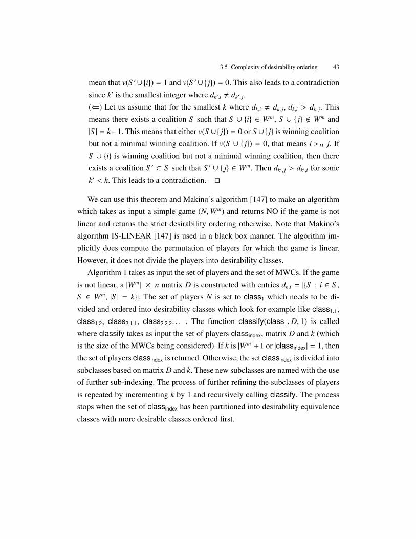
3.5 Complexity of desirability ordering 43
mean that v(S ′∪{i}) = 1 and v(S ′∪{ j}) = 0. This also leads to a contradictionsince k′ is the smallest integer where dk′,i , dk′, j.(⇐) Let us assume that for the smallest k where dk,i , dk, j, dk,i > dk, j. Thismeans there exists a coalition S such that S ∪ {i} ∈ Wm, S ∪ { j} < Wm and|S | = k−1. This means that either v(S ∪{ j}) = 0 or S ∪{ j} is winning coalitionbut not a minimal winning coalition. If v(S ∪ { j}) = 0, that means i �D j. IfS ∪ {i} is winning coalition but not a minimal winning coalition, then thereexists a coalition S ′ ⊂ S such that S ′ ∪ { j} ∈ Wm. Then dk′, j > dk′,i for somek′ < k. This leads to a contradiction. ut
We can use this theorem and Makino’s algorithm [147] to make an algorithmwhich takes as input a simple game (N,Wm) and returns NO if the game is notlinear and returns the strict desirability ordering otherwise. Note that Makino’salgorithm IS-LINEAR [147] is used in a black box manner. The algorithm im-plicitly does compute the permutation of players for which the game is linear.However, it does not divide the players into desirability classes.
Algorithm 1 takes as input the set of players and the set of MWCs. If the gameis not linear, a |Wm| × n matrix D is constructed with entries dk,i = |{S : i ∈ S ,S ∈ Wm, |S | = k}|. The set of players N is set to class1 which needs to be di-vided and ordered into desirability classes which look for example like class1.1,class1.2, class2.1.1, class2.2.2. . . . The function classify(class1,D, 1) is calledwhere classify takes as input the set of players classindex, matrix D and k (whichis the size of the MWCs being considered). If k is |Wm|+1 or |classindex| = 1, thenthe set of players classindex is returned. Otherwise, the set classindex is divided intosubclasses based on matrix D and k. These new subclasses are named with the useof further sub-indexing. The process of further refining the subclasses of playersis repeated by incrementing k by 1 and recursively calling classify. The processstops when the set of classindex has been partitioned into desirability equivalenceclasses with more desirable classes ordered first.

44 3 Complexity of comparison of influence of players in simple games
Algorithm 1 Strict-desirability-ordering-of-simple-gameInput: Simple game v = (N,Wm) where N = {1, . . . , n} and Wm(v) = {S 1, . . . , S |Wm |} .
Output: NO if v is not linear. Otherwise output desirability equivalence classes starting from most desirable,
if v is linear.
1: X = IS-LINEAR(Wm)
2: if X = NO then3: return NO
4: else5: Initialize an |Wm| × n matrix D with entries di, j = 0 for all i and j in N
6: for i = 1 to |Wm| do7: for each player x in S i do8: d|S i |,x ← d|S i |,x + 1
9: end for10: end for11: class1 ← N
12: return classify(class1,D, 1)
13: end if
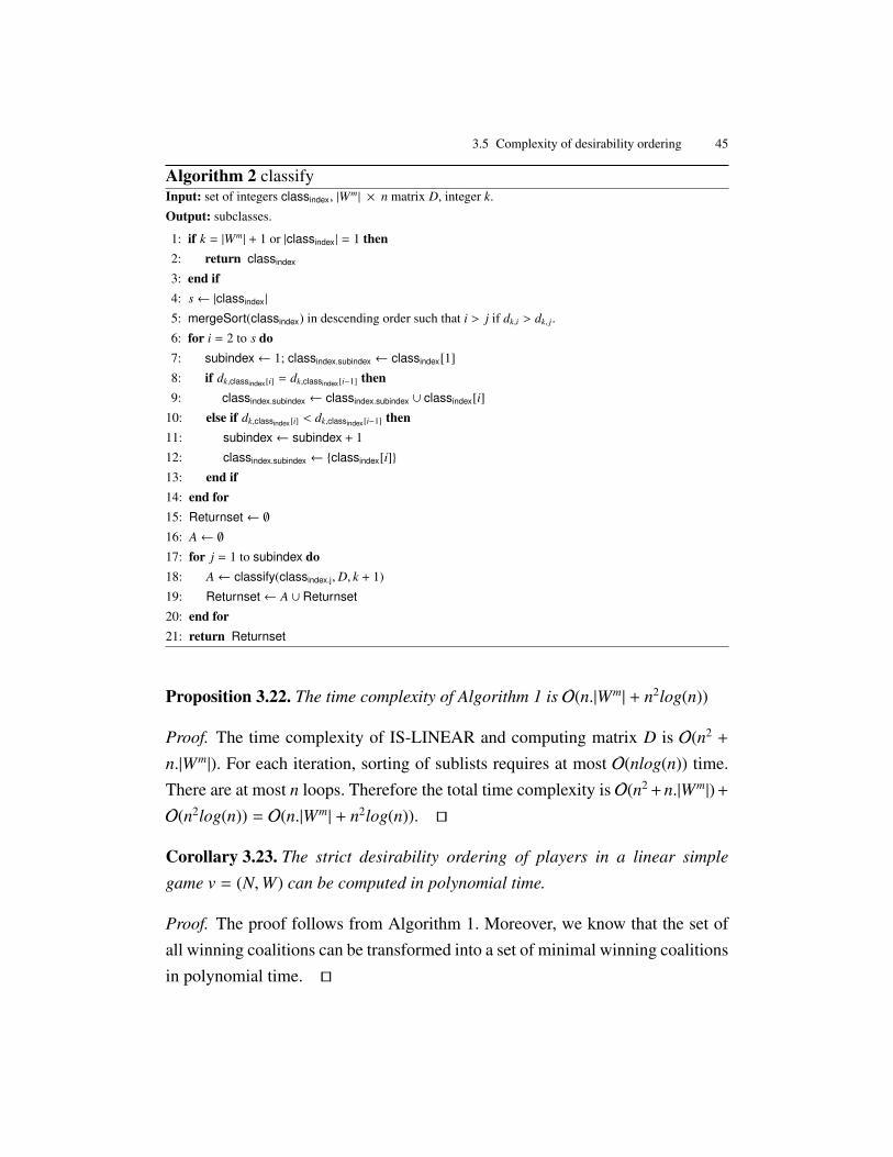
3.5 Complexity of desirability ordering 45
Algorithm 2 classifyInput: set of integers classindex, |Wm| × n matrix D, integer k.
Output: subclasses.
1: if k = |Wm| + 1 or |classindex| = 1 then2: return classindex
3: end if4: s← |classindex|
5: mergeSort(classindex) in descending order such that i > j if dk,i > dk, j.
6: for i = 2 to s do7: subindex← 1; classindex.subindex ← classindex[1]
8: if dk,classindex[i] = dk,classindex[i−1] then9: classindex.subindex ← classindex.subindex ∪ classindex[i]
10: else if dk,classindex[i] < dk,classindex[i−1] then11: subindex← subindex + 1
12: classindex.subindex ← {classindex[i]}
13: end if14: end for15: Returnset← ∅
16: A← ∅
17: for j = 1 to subindex do18: A← classify(classindex.j,D, k + 1)
19: Returnset← A ∪ Returnset
20: end for21: return Returnset
Proposition 3.22. The time complexity of Algorithm 1 is O(n.|Wm| + n2log(n))
Proof. The time complexity of IS-LINEAR and computing matrix D is O(n2 +
n.|Wm|). For each iteration, sorting of sublists requires at most O(nlog(n)) time.There are at most n loops. Therefore the total time complexity is O(n2 + n.|Wm|) +
O(n2log(n)) = O(n.|Wm| + n2log(n)). ut
Corollary 3.23. The strict desirability ordering of players in a linear simple
game v = (N,W) can be computed in polynomial time.
Proof. The proof follows from Algorithm 1. Moreover, we know that the set ofall winning coalitions can be transformed into a set of minimal winning coalitionsin polynomial time. ut
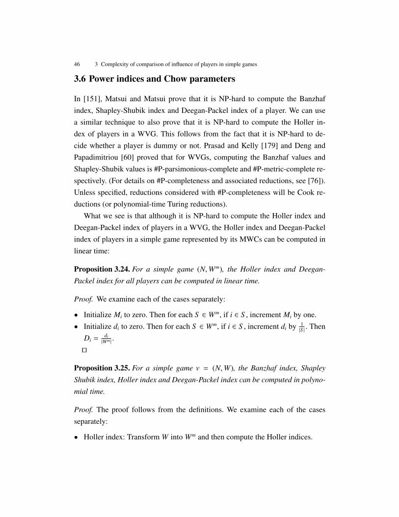
46 3 Complexity of comparison of influence of players in simple games
3.6 Power indices and Chow parameters
In [151], Matsui and Matsui prove that it is NP-hard to compute the Banzhafindex, Shapley-Shubik index and Deegan-Packel index of a player. We can usea similar technique to also prove that it is NP-hard to compute the Holler in-dex of players in a WVG. This follows from the fact that it is NP-hard to de-cide whether a player is dummy or not. Prasad and Kelly [179] and Deng andPapadimitriou [60] proved that for WVGs, computing the Banzhaf values andShapley-Shubik values is #P-parsimonious-complete and #P-metric-complete re-spectively. (For details on #P-completeness and associated reductions, see [76]).Unless specified, reductions considered with #P-completeness will be Cook re-ductions (or polynomial-time Turing reductions).
What we see is that although it is NP-hard to compute the Holler index andDeegan-Packel index of players in a WVG, the Holler index and Deegan-Packelindex of players in a simple game represented by its MWCs can be computed inlinear time:
Proposition 3.24. For a simple game (N,Wm), the Holler index and Deegan-
Packel index for all players can be computed in linear time.
Proof. We examine each of the cases separately:
• Initialize Mi to zero. Then for each S ∈ Wm, if i ∈ S , increment Mi by one.• Initialize di to zero. Then for each S ∈ Wm, if i ∈ S , increment di by 1
|S | . ThenDi = di
|Wm |.
ut
Proposition 3.25. For a simple game v = (N,W), the Banzhaf index, Shapley
Shubik index, Holler index and Deegan-Packel index can be computed in polyno-
mial time.
Proof. The proof follows from the definitions. We examine each of the casesseparately:
• Holler index: Transform W into Wm and then compute the Holler indices.

3.6 Power indices and Chow parameters 47
• Deegan-Packel: Transform W into Wm and then compute the Deegan-Packelindices.
• Banzhaf index: Initialize Banzhaf values of all players to zero. For each S ∈
W, check if the removal of a player results in S becoming losing (not a memberof W). In that case increment the Banzhaf value of that player by one.
• Shapley-Shubik index: Initialize Shapley values of all players to zero. Foreach S ∈ W, check if the removal of a player results in S becoming losing(not a member of W). In that case increment the Shapley value of the playerby (|S | − 1)!(n − |S |)!.
The time complexity for all cases is polynomial in the order of the input. ut
For a simple game (N,Wm), listing W the winning coalitions may take timeexponential in the number of players. For example, let there be only one minimalwinning coalition S which contains players 1, . . . , dn/2e. Then the number ofwinning coalitions to list is exponential in the number of players. Moreover, if|Wm| > 1, minimal winning coalitions can have common supersets. It is shownbelow that for a simple game (N,Wm), even counting the total number of winningcoalitions is #P-complete. Moreover, whereas it is possible in polynomial time tocheck if a player has zero voting power (a dummy) as seen in Proposition 3.13or whether it has voting power 1 (dictator) as seen in Proposition 3.15, it is #P-complete to find the actual Banzhaf or Shapley-Shubik index of the player.
Proposition 3.26. For a simple game v = (N,Wm), the problem of computing the
Banzhaf values of players is #P-complete.
Proof. The problem is clearly in #P. We prove the #P-hardness of the problem byproviding a reduction from the problem of computing |W |. Ball and Provan [30]proved that computing |W | is #P-complete. Their proof is in the context of relia-bility functions so we first give the proof in terms of simple games. It is known[181] that counting the number of vertex covers is #P-complete (a vertex coverin a graph G = (V, E) is a subset C of V such that every edge in E has at leastone endpoint in C). Now take a simple game v = (N,Wm) where for any S ∈ Wm,|S | = 2. Game v has a one-to-one correspondence with a graph G = (V, E) such

48 3 Complexity of comparison of influence of players in simple games
that N = V and {i, j} ∈ Wm if and only if {i, j} ∈ E(G). For a losing coalition,the set of players that do not belong to the losing coalition must correspond to avertex cover of G
In that case the total number of losing coalitions in v is equal to the number ofvertex covers of G. Therefore the total number of winning coalitions is equal to2n−(number of vertex covers of G) and computing |W | is #P-complete.
Now we take a game v = (N,Wm) and convert it into another game v′ = (N ∪{x},Wm(v′)) where Wm(v′) = {S ∪ {x}|S ∈ Wm(v)}. In that case computing |W(v)|is equivalent to computing the Banzhaf value of player x in game v′. Therefore,computing Banzhaf values of players in games represented by MWCs is #P-hard.ut
It follows from the proof that computing the power of collectivity to act( |W |2n )and the Chow parameters for a simple game (N,Wm) is #P-complete. Goldbergremarks in the conclusion of [100] that computing the Chow parameters of aWVG is #P-complete. It is easy to prove this. We remember that the Chow pa-rameter for player i is dented by |Wi| orωi. The problem of computing |W | and |Wi|
for any player i is in #P since a winning coalition can be verified in polynomialtime. It is easy to reduce in polynomial time the counting version of the SUBSET-SUM problem to counting the number of winning coalitions. Moreover, for anyWVG v = [q; w1, . . . ,wn], |W(v)| is equal to |Wx(v′)| where v′ is [q; w1, . . . ,wn, 0].Therefore computing |Wi| and |W | for a WVG is #P-complete.
We remember that ηi is the Banzhaf value of a game, ωi is the number of win-ning coalitions which include player i and ω denotes the total number of winningcoalitions.
Lemma 3.27.ηi = 2ωi − ω
Proof. Let ωi− be the number of those winning coalitions which do not includei. Then, the total number of winning coalitions is ω = ωi + ωi− . The number ofwinning coalitions which include i is equal to the number of losing coalitionsfor which i is critical plus the number of coalitions which do not include i but are
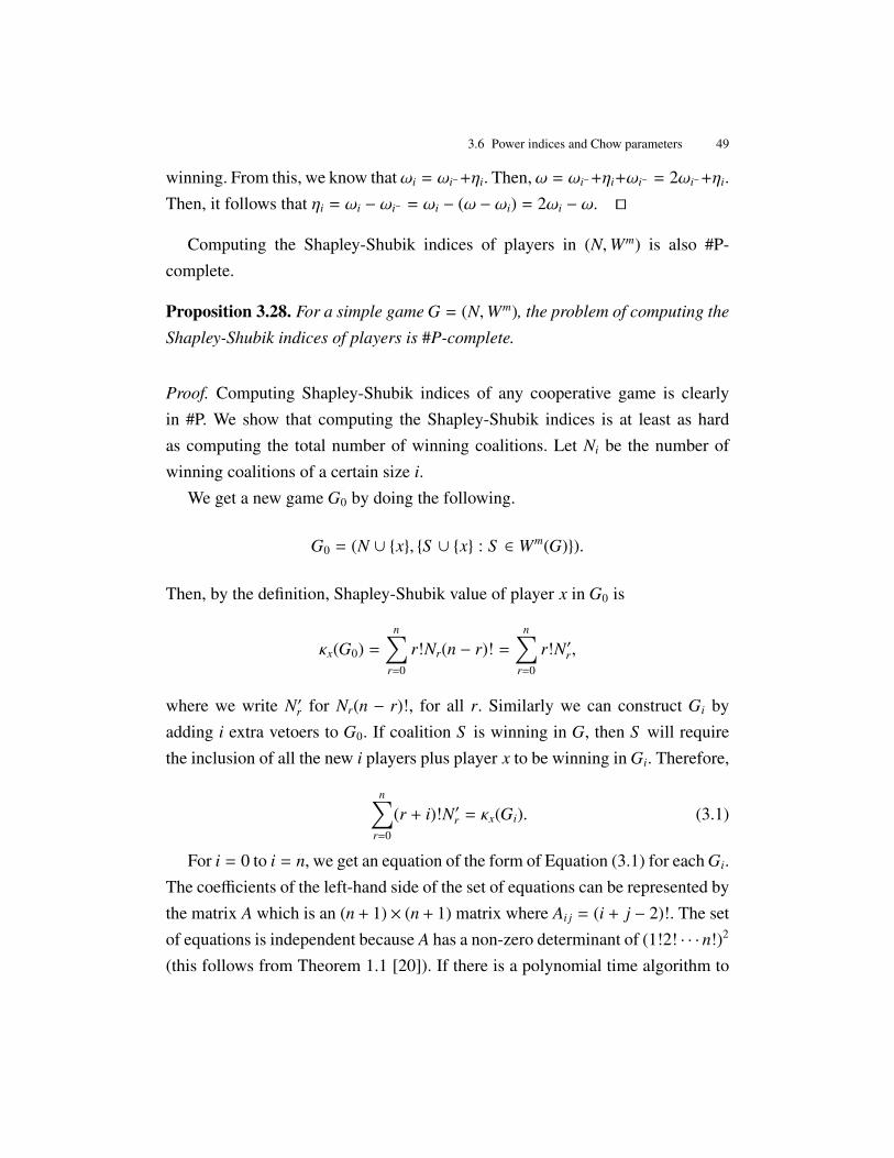
3.6 Power indices and Chow parameters 49
winning. From this, we know thatωi = ωi−+ηi. Then,ω = ωi−+ηi+ωi− = 2ωi−+ηi.Then, it follows that ηi = ωi − ωi− = ωi − (ω − ωi) = 2ωi − ω. ut
Computing the Shapley-Shubik indices of players in (N,Wm) is also #P-complete.
Proposition 3.28. For a simple game G = (N,Wm), the problem of computing the
Shapley-Shubik indices of players is #P-complete.
Proof. Computing Shapley-Shubik indices of any cooperative game is clearlyin #P. We show that computing the Shapley-Shubik indices is at least as hardas computing the total number of winning coalitions. Let Ni be the number ofwinning coalitions of a certain size i.
We get a new game G0 by doing the following.
G0 = (N ∪ {x}, {S ∪ {x} : S ∈ Wm(G)}).
Then, by the definition, Shapley-Shubik value of player x in G0 is
κx(G0) =
n∑r=0
r!Nr(n − r)! =
n∑r=0
r!N′r,
where we write N′r for Nr(n − r)!, for all r. Similarly we can construct Gi byadding i extra vetoers to G0. If coalition S is winning in G, then S will requirethe inclusion of all the new i players plus player x to be winning in Gi. Therefore,
n∑r=0
(r + i)!N′r = κx(Gi). (3.1)
For i = 0 to i = n, we get an equation of the form of Equation (3.1) for each Gi.The coefficients of the left-hand side of the set of equations can be represented bythe matrix A which is an (n + 1)× (n + 1) matrix where Ai j = (i + j − 2)!. The setof equations is independent because A has a non-zero determinant of (1!2! · · · n!)2
(this follows from Theorem 1.1 [20]). If there is a polynomial time algorithm to

50 3 Complexity of comparison of influence of players in simple games
compute the Shapley-Shubik index of each edge in a simple graph, then we cancompute the right-hand side of each equation corresponding to Gi.
The biggest possible number in the equation is less than (2n)! and can be rep-resented efficiently. This follows from the fact that n! ≤ nn and hence to represent(2n)!, one will use at most log2((2n)2n) = 2n(1 + log2 n) ≤ 3n log2 n bits.
We can use Gaussian elimination to solve the set of linear equation in O(n3)time. Moreover, each number that occurs in the algorithm can also be stored ina number of bits quadratic of the input size (Theorem 4.10 [123]). If there isan algorithm polynomial in the number of edges to compute the Shapley-Shubikindex of all edges in the graph, then each Ni can be computed in polynomial time.ut
A representation of a simple game is considered reasonable if, for a simplegame (N, v), the new game (N∪{x}, v′) where v(S ) = 1 if and only if v′(S ∪{x}) =
1, can also be represented with only a polynomial blowup. The following theoremcharacterizes the relation between the computational complexity of the Banzhafvalue and the Shapley-Shubik indices.
Theorem 3.29. For a simple game with a reasonable representation, if computing
the Banzhaf values is #P-complete, then computing the Shapley-Shubik indices is
#P-complete.
Proof. Assume that computing the Banzhaf values is #P-complete. The prooftechnique in Proposition 3.6 can be used to show that for any reasonable represen-tation of the simple game, a polynomial time algorithm to compute the Shapley-Shubik indices implies a polynomial time algorithm to compute the Banzhaf in-dices.
It is first proved that if computing the Banzhaf values of players in a reasonablerepresentation is #P-complete, then computing ω, the total number of winningcoalitions is #P-complete. Assume that there is an oracle which can compute ωof simple game (N, v) in polynomial time. Since ηi(N, v) = ω(N, v)−ω(N \ {i}, v),ηi(N, v) can be computed in polynomial time. Therefore, computing ω(N, v) is#P-complete. However, we saw that if there is an oracle to compute the Shapley-Shubik indices of a simple game (in a reasonable representation) in polynomial
3.7 Conclusion 51
time, then Nis can be computed in polynomial time. Since∑n
j=1 Ni = ω, ω can becomputed in polynomial time. ut
As a corollary, we strengthen the complexity results for two other networkgames which are representations of simple games and answer open questionsabout the complexity of a host of skill based games:
Corollary 3.30. Computing Shapley value is #P-complete for
1. Threshold Network Flow Games [26]
2. Vertex Connectivity Games [27]
3. STSG (Single Task Skill Game), TCSG (Task Count Skill Game), WTSG
(Weighted Task Skill Game), TCSG-T (Task Count Skill Game with thresh-
olds) and WTSG-T (Weighted Task Skill Game with thresholds) [25]
Proof. For the given games, computing Banzhaf values is #P-complete. It iseasy to see that the games Threshold Network Flow Games, Vertex ConnectivityGames, STSG (Single Task Skill Game), TCSG-T (Task Count Skill Game withthresholds) and WTSG-T (Weighted Task Skill Game with thresholds) are sim-ple games with reasonable representations. Also, TCSG (Task Count Skill Game)and WTSG (Weighted Task Skill Game) are generalizations of the STSG (SingleTask Skill Game). ut
As we will see later, the proof technique of Theorem 3.29 will be used in theproof of Proposition 12.5.
3.7 Conclusion
A summary of results has been listed in Table 3.1. A question mark indicates thatthe specified problem is still open. It is conjectured that it is NP-hard to computeBanzhaf indices for a simple game represented by (N,Wm). It is found that al-though WVG, MWVG and even (N,Wm) are relatively compact representationsof simple games, some of the important information encoded in these representa-tions can apparently only be accessed by unraveling these representations. There

52 3 Complexity of comparison of influence of players in simple games
is a need for a greater examination of transformations of simple games into com-pact representations.
Table 3.1. Complexity of comparing players
(N,W) (N,Wm) WVG MWVG
IDENTIFY-DUMMIES P linear NP-hard NP-hardIDENTIFY-VETOERS linear linear linear linearIDENTIFY-PASSERS linear linear linear linearIDENTIFY-DICTATOR linear linear linear linearCHOW PARAMETERS linear #P-complete #P-complete #P-completeIS-LINEAR P P (Always linear) NP-hardDESIRABILITY-ORDERING P P P NP-hardSTRICT-DESIRABILITY P P NP-hard NP-hardBANZHAF-VALUES P #P-complete #P-complete #P-completeBANZHAF-INDICES P ? NP-hard NP-hardSHAPLEY-SHUBIK-VALUES P #P-complete #P-complete #P-completeSHAPLEY-SHUBIK-INDICES P #P-complete #P-complete #P-completeHOLLER-INDICES P linear NP-hard NP-hardDEEGAN-PACKEL-INDICES P linear NP-hard NP-hard

4
Classification of computationally tractable weightedvoting games
In order to distinguish what is most simple from what is complex, and to
deal with things in an orderly way, what we must do, whenever we have
a series in which we have directly deduced a number of truths one from
another, is to observe which one is most simple, and how far all the others
are removed from this—whether more, or less, or equally.
- Descartes (Rule VI, Rules for the Direction of the Mind)
Abstract It is well known that computing Banzhaf indices in a weighted votinggame is #P-complete. We give a comprehensive classification of weighted votinggames which can be solved in polynomial time. Among other results, we providea polynomial (O(k( n
k )k)) algorithm to compute the Banzhaf indices in weightedvoting games in which the number of weight values is bounded by k. Compu-tational results concerning weighted voting games with special distributions ofweights are also presented.
4.1 Introduction
4.1.1 Motivation and outline
The Banzhaf index is considered the most suitable power index by voting powertheorists ([132] and [82]). As mentioned before in Chapter 3, the computationalcomplexity of computing Banzhaf indices in WVGs is well studied. Prasad and

54 4 Classification of computationally tractable weighted voting games
Kelly [179] show that the problem of computing the Banzhaf values of playersis #P-complete. It is even NP-hard to identify a player with zero voting power ortwo players with same Banzhaf indices [151].
Klinz and Woeginger [121] devised the fastest exact algorithm to computeBanzhaf indices in a WVG. In the algorithm, they applied a partitioning approachthat dates back to Horowitz and Sahni [108]. However the complexity of the algo-rithm is stillO(n22
n2 ). In this chapter, we restrict our analysis to exact computation
of Banzhaf indices instead of examining approximate solutions. We show that al-though computing Banzhaf indices of WVGs is a hard problem in general, it iseasy for various classes of WVGs, e.g., for WVGs with a bounded number ofweight values, an important sub-class of WVGs.
The outline of the chapter is as following. Section 4.2 identifies WVGs inwhich Banzhaf indices can be computed in constant time. In Section 4.3, we ex-amine WVGs with a bounded number of weight values, and provide algorithmsto compute the Banzhaf indices. Section 4.4 examines WVGs with special weightdistributions. Section 4.5 considers WVGs with integer weights. Section 4.6 pro-vides a survey of approximate approaches to computing power indices in WVGs.We conclude with some open problems in the final section.
Generally, 12
∑1≤i≤n wi < q ≤
∑1≤i≤n wi so that there can be no two disjoint
winning coalitions. Such weighted voting games are proper.The problem of computing the Banzhaf indices of a WVG can be defined
formally as following:Name: BI-WVGInstance: WVG, v = [q; w1, ...,wn]Question: What are the Banzhaf indices of the players?
Here, we will suppose that arithmetic operations on O(n)-digit numbers canbe done in constant time.

4.2 Extreme cases 55
4.2 Extreme cases
If the WVG v is [q; u, u, . . . , u︸ ︷︷ ︸n
], then the Banzhaf indices β1, ... , βn are equal
to 1/n. The Banzhaf indices can be found in constant time, and the followingtheorem gives the actual number of swings for each player.
Theorem 4.1. In a WVG with n equal weights, u, each player is critical in(
n−1dq/ue−1
)coalitions. Moreover, the total number of winning coalitions w is
∑ni=dq/ue
(ni
).
Proof. The minimum number of players needed to form a winning coalition isdq/ue. A player is critical in a coalition if there are exactly dq/ue−1 other playersin the coalition. There are
(n−1dq/ue−1
)such coalitions. There are
(ni
)coalitions of size
i and such a coalition is winning if i ≥ dq/ue. ut
Also, in a WVG with n equal weights u, the probabilistic Banzhaf index ofeach player is then
(n−1dq/ue−1
)/2n−1. We can also compute Coleman’s power of the
collectivity to act, A, which is equal to w2n .
A dictator is a player who is present in every winning coalition and absentfrom every losing coalition. This means that the player 1 with the biggest weightis a dictator if and only if w1 ≥ q and
∑2≤i≤n wi < q. In that case, β1 = 1 and
βi = 0 for all i > 1.If 0 < q ≤ wn then the only minimal winning coalitions are all the singleton
coalitions. So there are n minimal winning coalitions and every player is criticalin one coalition. Thus, for all i, βi = 1/n and the Banzhaf indices can be found inconstant time (i.e., O(1)). Moreover, the probabilistic Banzhaf index β
′
i = 1/2n−1
for all i, and Coleman’s power of collectivity to act A = 2n−12n
If q ≥∑
1≤i≤n wi − wn, then the only minimal winning coalition is {1, 2, . . . , n}and it becomes losing if any player gets out of the coalition. Thus the weightedvoting game acts like the unanimity game. Then for all i, βi = 1/n. The Banzhafindices can be found in constant time (i.e., O(1)). Moreover, for all i, β
′
i = 1/2n−1
and A = 1/2n.

56 4 Classification of computationally tractable weighted voting games
4.3 Bounded number of weight values
In this section we estimate the time complexity of several algorithms. We startoff with the case when all weights except one are equal and give exact formulasfor the Banzhaf indices. We then use this as a warm up exercise to consider moregeneral cases where there are 2 weight values and then k weight values.
4.3.1 All weights except one are equal
We start off with the case when all weights except one are equal.
Theorem 4.2. Let v be a WVG, [q; wa,wb, ...,wb], where there is wa and m weights
of value wb, where wb < q. Let x be d q−wawbe and y = dq/wbe. Then the total
number of coalitions in which a player with weight wb is critical is(
m−1y−1
)+
(m−1
x
).
Moreover, the number of coalitions in which the player with weight wa is critical
is∑Min(y−1,m)
i=x
(mi
).
Proof. A player with weight wb is critical in 2 cases:
1. It makes a winning coalition with other players with weight wb only. Let y
be the minimum number of players with weight wb which form a winningcoalition by themselves. Thus y = dq/wbe. The number of such coalitions inwhich a player with weight wb can be critical is
(m−1y−1
).
2. It makes a winning coalition with the player with weight wa and none or some
players with weight wb. Let x be the minimum number of players with weightwb which can form a winning coalition with the inclusion of the player withweight wa. Thus x = d
q−wawbe. Then, the number of such coalitions in which a
player with weight wb can be critical is(
m−1x
).
The total number of swings for a player with weight wb is thus(
m−1y−1
)+
(m−1
x
).
The player with weight wa is critical if it forms a winning a coalition withsome players with weight wb but the coalition becomes losing with its exclusion.The player with weight wa can prove critical in coalition with varying number ofplayers with weight wb. The maximum number of players with weight wb withwhich it forms a winning coalition and is also critical is y−1 in case y ≤ m and m
4.3 Bounded number of weight values 57
in case y > m. Therefore the total number of coalitions in which the player withweight wa is critical is
∑Min(y−1,m)i=x
(mi
). ut
4.3.2 Only two different weight values
Unlike Theorem 4.2, we do not give a short formula for the Banzhaf values in thenext theorem. However Theorem 4.3 considers a more general case than Theo-rem 4.2. As we shall we later Theorem 4.2 provides us with an idea to considerthe case of k weight values.
Theorem 4.3. For a WVG with n players and only two weight values, the Banzhaf
indices and numbers of swings can be computed in O(n2) time.
Proof. We look at a WVG, v = [q; wa, ...wa,wb, ...wb], where there are na playerswith weight wa and nb players with weight wb. We analyse the situation when aplayer with weight wa proves to be critical in a coalition which has i other playerswith weight wa and the rest with weight wb. Then the minimum number of playerswith weight wb required is d q−(i+1)wa
wbe. Moreover the maximum number of players
with wb is d q−iwawbe−1. Therefore j, the number of players with weight wb, satisfies
the following inequality: x1(i) = dq−(i+1)wa
wbe ≤ j ≤ Min(d q−iwa
wbe − 1, nb) = x2(i). Let
Ai =(
na−1i
), and let Bi =
∑x2(i)j=x1(i)
(nbj
). We define, the maximum possible number of
extra players with weight a, to be maxa = Min(dq/wae − 1, na − 1). Then the totalnumber of swings of the player with weight wa is
∑maxai=0 AiBi. The total number
of swings for a player with weight wb can be computed by a symmetric method.ut
We can devise an algorithm (Algorithm 4) from the method outlined in theproof.

58 4 Classification of computationally tractable weighted voting games
Algorithm 3 SwingsFor2ValueWVGInput: v = [q; (na,wa), (nb,wb)].
Output: Total swings of a player with weight wa.
1: swingsa ← 0
2: maxa← Min(dq/wae − 1, na − 1)
3: for i = 0 to maxa do4: x1(i)← d q−(i+1)wa
wbe
5: x2(i)← Min(d q−i(wa)wbe − 1, nb)
6: Ai ←(
na−1i
)7: if x1(i) > nb then8: Bi ← 0
9: else if x2(i) < 0 then10: Bi ← 0
11: else12: Bi ← 0
13: for j = x1(i) to x2(i) do14: Bi ← Bi +
(nbj
)15: end for16: end if17: swingsa = swingsa + AiBi
18: end for19: return swingsa
Algorithm 4 BIsFor2ValueWVGInput: v = [q; (na,wa), (nb,wb)].
Output: Banzhaf indices, β = (βa, βb).
1: swingsa = SwingsFor2ValueWVG(v)
2: v′ = [q; (nb,wb), (na,wa)]
3: swingsb = SwingsFor2ValueWVG(v′)
4: totalswings = naswingsa + nbswingsb
5: βa =swingsa
totalswings
6: βb =swingsb
totalswings
7: return (βa, βb)
The algorithm for 2 weight values serves as warm-up for the general case of k
weight values in the next section.

4.3 Bounded number of weight values 59
4.3.3 k weight values
Theorem 4.4. The problem of computing Banzhaf indices of a WVG with k pos-
sible values of the weights is solvable in O(nk).
Proof. We can represent a WVG v with k weight classes as follows:
[q; (n1,w1), (n2,w1), ..., (nk,wk)]
where ni is the number of players with weights wi for i = 1, . . . , k. Here, weextend Algorithm 4 to Algorithm 6 for k weight classes.
We can write v′ as [q; (1,w0), (n1 − 1,w1), ..., (nk,wk)] where w0 = w1. Thismakes it simpler to write a recursive function to compute the number of swingsof player with weight w0. Let Ai1,i2,...,im be the number of swings for w0 wherethere are i j players with weight w j in the coalition for 1 ≤ j ≤ m.
Then
Ai1,i2,...,ik =
(
n1−1i1
)(Πk
j=2
(n ji j
)) if q − w0 ≤
∑kj=1 i jw j < q
0 otherwise.
Now for 1 ≤ m ≤ k,
Ai1,i2,...,im−1 =∑
im
Ai1,i2,...,im .
Here the summation is taken over all values of im for which the contribution isnon-zero. Explicitly, this range is given by
Max(
q − w0 −∑m−1
j=1 i jw j −∑k
j=m+1 n jw j
wm
, 0) ≤ im ≤ Min(
q −∑m−1
j=1 i jw j
wm
−1, nm).
The total number of swings of the player with weight w0 is then Aε .
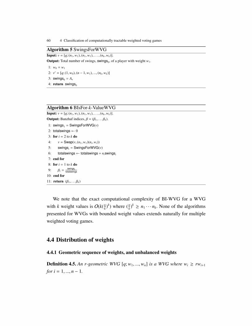
60 4 Classification of computationally tractable weighted voting games
Algorithm 5 SwingsForWVGInput: v = [q; (n1,w1), (n1,w1), . . . , (nk,wk)].
Output: Total number of swings, swings0, of a player with weight w1.
1: w0 = w1
2: v′ = [q; (1,w0), (n − 1,w1), ..., (nk,wk)]
3: swings0 = Aε
4: return swings0
Algorithm 6 BIsFor-k-ValueWVGInput: v = [q; (n1,w1), (n1,w1), . . . , (nk,wk)].
Output: Banzhaf indices, β = (β1, . . . βk).
1: swings1 = SwingsForWVG(v)
2: totalswings← 0
3: for i = 2 to k do4: v = Swap(v, (n1,w1)(ni,wi))
5: swingsi = SwingsForWVG(v)
6: totalswings← totalswings + niswingsi
7: end for8: for i = 1 to k do9: βi =
swingsitotalswings
10: end for11: return (β1, . . . βk)
We note that the exact computational complexity of BI-WVG for a WVGwith k weight values is O(k(n
k )k) where (nk )k≥ n1 · · · nk. None of the algorithms
presented for WVGs with bounded weight values extends naturally for multipleweighted voting games.
4.4 Distribution of weights
4.4.1 Geometric sequence of weights, and unbalanced weights
Definition 4.5. An r-geometric WVG [q; w1, ...,wn] is a WVG where wi ≥ rwi+1
for i = 1, ..., n − 1.
4.4 Distribution of weights 61
We observe that in a 2-geometric WVG (such as [q; 2n, 2n−1, ..., ]), for anytarget sum of a coalition, we can use a greedy approach, trying to put biggerweights first, to come as close to the target as possible. This greedy approachwas first identified by Chakravarty, Goel and Sastry [43] for a broader categoryof weighted voting games in which weights are unbalanced:
Definition 4.6. An unbalanced WVG is a WVG such that, for 1 ≤ j ≤ n, w j >
w j+1 + w j+2... + wn.
Example 4.7. The game [22; 18, 9, 4, 2, 1] is an example of an unbalanced WVGwhere each weight is greater than the sum of the subsequent weights.
Chakravarty, Goel and Sastry [43] showed that the greedy approach for un-balanced WVG with integer weights can help to compute all Banzhaf indicesin O(n). We notice that the same algorithm can be used for an unbalanced WVGwith real weights without any modification. In fact it is this property of ‘geometricweights’ being unbalanced which is the reason that we can find suitable coalitionsfor target sums so efficiently. We characterise those geometric sequences whichgive unbalanced WVGs:
Theorem 4.8. If r ≥ 2 then every r-geometric WVG is unbalanced.
Proof. Let v be an r-geometric WVG. We prove by induction that w j > w j+1 +
. . . + wn. This is true for j = n. Suppose it is true for all i, j + 1 ≤ i ≤ n. Since v
is r-geometric, w j ≥ 2w j+1. But, 2w j+1 = w j+1 + w j+1 > w j+1 + w j+2 + . . . + wn.Therefore v is unbalanced. ut
Corollary 4.9. For an r-geometric WVG v where r ≥ 2, the Banzhaf indices of
players in v can be computed in O(n) time.
Proof. Since the condition of r ≥ 2 makes v an unbalanced WVG, then we canuse the greedy algorithm from [43] which computes the Banzhaf indices in O(n).ut
Definition 4.10. A WVG is a k-unbalanced WVG if, for 1 ≤ j ≤ n, w j > w j+k +
· · · + wn. So an unbalanced WVG is ‘1-unbalanced’.

62 4 Classification of computationally tractable weighted voting games
Note that an r-geometric WVG is 2-unbalanced when r ≥ 1+√
52 ≈ 1.61803... =
ϕ, the golden ratio, since then
1r2 +
1r3 + · · · <
1r(r − 1)
≤ 1 since r(r − 1) ≥ ϕ(ϕ − 1) = 1.
We check whether 2-unbalanced WVGs have properties similar to those ofunbalanced WVGs.
Example 4.11. Consider a WVG v with 2m players and weights
3m−1, 3m−1, . . . , 3 j, 3 j, . . . , 3, 3, 1, 1.
It is easy to see that∑ j−1
i=0 2 · 3i < 3 j, so the game is 2-unbalanced.
In the unbalanced game, for each target coalition sum, there is either one cor-responding coalition or none. This does not hold for 2-unbalanced WVGs. InExample 4.12 with target total 1 + 3 + · · ·+ 3m−1 = 1
2 (3m − 1), there are exactly 2m
coalitions which give this target, namely those coalitions with exactly one playerout of each equal pair.
We prove that even for the class of 2-unbalanced (instead of simply unbal-anced WVGs) the problem of computing Banzhaf indices becomes NP-hard.
Theorem 4.12. BI-WVG is NP-hard for the class of 2-unbalanced WVGs .
Proof. We will use a reduction from the following NP-hard problem:
Name: SUBSET SUM
Instance: z1, . . . , zm, T ∈ N.Question: Are there x js in {0, 1} so that
∑mj=1 x jz j = T?
For the reduction from SUBSET SUM, we scale and modify the weights fromthe WVG v of Example 4.12. For any instance I = {z1, . . . , zm,T } of SUBSETSUM, we will define a game vI with 2m + 1 players. Let Z = 1 +
∑mj=1 z j, and we
may assume that T < Z. Whereas v had pairs of weights 3 j, 3 j for 0 ≤ j ≤ m − 1,

4.4 Distribution of weights 63
in vI there is one “unit player” with weight 1 and 2m pairs of players with weights3 jZ, 3 jZ + z j for 0 ≤ j ≤ m − 1. The quota for vI is 1
2 (3m − 1)Z + T + 1. The unitplayer has nonzero Banzhaf index if and only if there exists a coalition amongthe other 2m players with weight exactly 1
2 (3m − 1)Z + T . We will show that todetermine this is equivalent to answering the SUBSET SUM instance I, and soeven this special case of BI-WVG is NP-hard.
In Example 4.12, it was necessary (and sufficient) for achieving the target totalof 1
2 (3m−1) to take exactly one player from each pair. In game vI , since∑m
j=1 z j <
Z, this is still a necessary condition for achieving the total of 12 (3m − 1)Z + T , and
whether or not there is such a selection achieving the total is exactly the conditionof whether there is a subset of the z js which sums to T . ut
4.4.2 Sequential weights
Definition 4.13. The set of weights {w1,w2, ...,wn} is sequential if
wn|wn−1|wn−2...|w1,
i.e. each weight is a multiple of the next weight.
Example 4.14. [32; 20, 10, 10, 5, 1, 1, 1] is an example of a WVG with sequentialweights.
Chakravarty, Goel and Sastry [43] show that Banzhaf indices can be computedin O(n2) time if the weights are sequential and they satisfy an additional domi-nance condition. The dominance conditions states that a weight in one weightclass should be more than the sum of weights of any subsequent weight class.
Definition 4.15. Let d1 > d2 > · · · > dr be the distinct values of weights
w1, . . . ,wn of a sequential set. Then dk = mkdk+1 where mk > 1, ∀k, 1 ≤ k < r.
Let Nk = {i | wi = dk} and nk = |Nk|. Then the dominance condition holds if
mk > nk+1 ∀k, 1 ≤ k < r.
We now define the alternative dominance condition for WVGs.

64 4 Classification of computationally tractable weighted voting games
Definition 4.16. Let d1 > d2 > · · · > dr be the distinct values of weights
w1, . . . ,wn of a sequential set. Let Nk = {i|wi = dk} and nk = |Nk|. Then the alterna-tive dominance condition holds if ∀ j ∈ Nk, 1 ≤ k < r, w j >
∑{wp | p ∈ Ni, i > k}.
We provide an alternative dominance condition for weights which are not nec-essarily sequential. It is easy to see that a 2-unbalanced WVG does not necessarilysatisfy the alternative dominance condition.
Definition 4.17. Let d1 > d2 > · · · > dr be the distinct values of weights
w1, . . . ,wn of a sequential set. Let Nk = {i|wi = dk} and nk = |Nk|. Then the alterna-tive dominance condition holds if ∀ j ∈ Nk, 1 ≤ k < r, w j >
∑{wp | p ∈ Ni, i > k}.
Proposition 4.18. Suppose a WVG v satisfies the alternative dominance condi-
tion. Then for v, BI-WVG has time complexity O(n2).
Proof. This follows from Theorem 10 in [43] where the proof is for a sequentialWVG which obeys the dominance condition. However we notice that since theargument in the proof can be made for any WVG which satisfies the alternativedominance condition, the proposition holds for v. ut
4.5 Integer weights
When all weights are integers, other methods may become applicable.
4.5.1 Moderate sized integer weights
Matsui and Matsui [151] prove that a dynamic programming approach providesa pseudo-polynomial algorithm to compute Banzhaf indices of all players withtime complexity O(n2q). Since q is less than
∑i∈N wi, the Banzhaf indices can be
computed in polynomial time if the weight sizes are moderate.
4.5.2 Polynomial number of coefficients in the generating function of theWVG
A generating function is a formal power series whose coefficients encode infor-mation about a sequence. Bilbao et al. [36] observe, for a WVG v = [q; w1, . . . ,wn],
4.6 Approximation approaches 65
that if the number of coalitions for which a player i is critical is bi = |{S ⊂ N :v(S ) = 0, v(S ∪{i}) = 1}| =
∑q−1k=q−wi
bik, where bi
k is the number of coalitions whichdo not include i and with total weight k, then the generating functions of the num-bers {bi
k} are given by Bi(x) =∏n
j=1, j,i(1+ xw j) = 1+bi1x+bi
2x2 + · · ·+biW−wi
xW−wi .This was first pointed out by Brams and Affuso [39].
Example 4.19. Let v = [6; 5, 4, 1] be a WVG.
• B1(x) = (1 + x4)(1 + x1) = 1 + x + x4 + x5
The coalitions in which player 1 is critical are {1, 2}, {1, 3}, {1, 2, 3}. Thereforeη1 = 3.
• B2(x) = (1 + x5)(1 + x1) = 1 + x + x5 + x6 The coalition in which player 2 iscritical is {1, 2}. Therefore η2 = 1.
• B3(x) = (1 + x5)(1 + x4) = 1 + x4 + x5 + x9
The coalition in which player 3 is critical is {1, 3}. Therefore η3 = 1.
Consequently, β1 = 3/5, β2 = 1/5 and β3 = 1/5.
The generating function method provides an efficient way of computingBanzhaf indices if the voting weights are moderate integers. Bilbao et al. [36]prove that the computational complexity of computing Banzhaf indices by gen-erating functions is O(n2C) where C is the number of non-zero coefficients in∏
1≤i≤n(1 + xw j). We note that C can be bounded by the sum of the weights butthe bound is not tight. C can be relatively small even if the weight values areexponential in n. Therefore if a WVG has a generating function in which thenumber of non-zero terms is polynomial in n, then the computational complexityof computing the Banzhaf indices is in P.
4.6 Approximation approaches
The earliest approximate algorithm for power indices was the Monte Carlo ap-proach by Mann and Shapley [148]. Owen [164, 165] devised an approach usingmultilinear extension(MLE) which provides an exact computation of power in-dices. The method has exponential time complexity. However the MLE approach

66 4 Classification of computationally tractable weighted voting games
can be utilized in large games for approximations using the central limit the-orem [135]. Leech [131] succinctly outlines the basic idea of approximationsusing Owen’s MLE approach. Holzman et al. [107] and then Freixas [87] pro-vide bounds for Owen’s MLE. Matsui and Matsui [151] in their survey of votingpower algorithms also include the Monte Carlo approach. However, they do notfocus on the analysis of the errors induced. Fatima et al. [80] propose a variationof Mann and Shapley’s [148] algorithm by treating the players’ weights insteadof the players’ numbers of swings as random variables. Bachrach et al. [22] sug-gest and analyse the randomized approximate algorithm to compute the Banzhafindex and the Shapley-Shubik index with a comprehensive theoretical analysis ofthe confidence intervals and errors induced.
4.7 Open problems & conclusion
Table 4.1 contains a summary of the algorithms or complexity results for differ-ent classes of WVGs. A&P refers to Aziz and Paterson. In this chapter we haveclassified WVGs for which Banzhaf indices can be computed in polynomial time.It would be interesting to identify further important classes of WVGs which haveless than exponential time complexity. The extensive literature on the SUBSET-SUM problem should offer guidance here. It appears an interesting question toanalyse the expected number of terms in the generating function for sequentialWVGs. Another challenging open problem is to devise an algorithm to computeexactly the Banzhaf indices of a general WVG in time complexity which is lessthan O(n22
n2 ).

4.7 Open problems & conclusion 67
Table 4.1. Complexity of WVG classes
WVG Class R/Z Complexity Time RemarksClass
General R/Z NP-Hard O(n21.415n) [121]Unbalanced R/Z P O(n) [43]k-Unbalanced(k ≥ 2) R/Z NP-Hard A&P [16]Sequential with dominance R/Z P O(n2) [43]Alternative dominance R/Z P O(n) A&P [16] + [43]Bounded(k) #(weight values) R/Z P O(nk) A&P [16]r-geometric R/Z P O(n) A&P [16] + [43]Moderate integer weights Z P O(n2q) [151]Moderate GF Z P O(n2C) [39], [36]

5
Multiple weighted voting games
In a capitalist democracy, there are essentially two methods by which so-
cial choices can be made: voting, typically to make “political decisions”,
and the market mechanism, typically used to make “economic decisions”.
- Kenneth J. Arrow (Social Choice and Individual Values [8])
Abstract We provide mathematical and computational properties of multiple
weighted voting games which are an extension of weighted voting games. Weanalyse the structure of multiple weighted voting games and some of their com-binatorial properties especially with respect to dictatorship, veto power, dummyplayers and Banzhaf indices. An illustrative Mathematica program to computevoting power properties of multiple weighted voting games is also provided.
5.1 Introduction
MWVGs are utilized in various situations. The treaty of Nice made the overallvoting games of the EU countries a triple majority weighed voting game with cer-tain additional constraints. MWVGs are useful in multi-criteria multi-agent sys-tems. We analyse combinatorial properties of multiple weighted voting games es-pecially with respect to dictatorship, veto power and dummy players. The chapteralso outlines algorithmic considerations when computing voting power of play-ers in multiple weighted voting games. In [77], the authors generalize multipleweighted voting games and consider boolean weighted voting games which are

70 5 Multiple weighted voting games
logical combinations of weighted voting games. However, we restrict out atten-tion to MWVGs which are the most common extension of WVGs.
5.2 MWVGs
In this section, we examine some standard properties of MWVGs which weredefined in Definitions 2.4.
5.2.1 Structure
We define S i as the set of coalitions not including player i. Then S i can be parti-tioned into three mutually exclusive sets:
S i = Wi(v) ∪Ci(v) ∪ Li(v)
where
• Wi(v) is the set of coalitions not including player i which are winning in themultiple game v
• Li(v) is the set of coalitions not including player i which are losing in themultiple game v even if player i joins the coalitions.
• Ci(v) is the set of coalitions not including player i which are losing in themultiple game v but winning in v if player i joins the coalitions.
The number of coalitions in which player i is critical in the multiple game v isηi(v) = |Ci(v)|. In a MWVG v = ∧v j, i is critical in a coalition S if
(∀ j : (S ∈ Ci(v j) ∨ S ∈ Wi(v j)) ∧ (∃ j : S ∈ Ci(v j))
We define W(v) as the set of winning coalitions in v and W(vi) as the set ofwinning coalitions in vi. In that case
W(v) = W(v1) ∩W(v2)... ∩W(vm)

5.3 Properties of MWVGs 71
Similarly if we define L(v) as the set of losing coalitions in v and L(vi) as theset of losing coalitions in vi. In that case
L(v) = L(v1) ∪ L(v2)... ∪ L(vm)
5.2.2 Trade robustness
Deineko and Woeginger [57] show that it is NP-hard to verify the dimension ofmultiple-weighted voting games. In [90], it is pointed out that the dimension of agame is at most the number of maximal losing coalitions. This kind of bound isnot very helpful though in estimating the actual dimension of a MWVG.
In Definition 3.6, swap-robust and trade-robust were defined. Taylor andZwicker [202] proved that a simple game is trade robust if and only if it is aWVG. However, MWVGs are not even swap-robust:
Example 5.1. Let (N, v) = (N, v1 ∧ v2) where v1 = [20; 18, 5, 0, 5, 5, 2, 5] and v2 =
[20; 0, 5, 18, 5, 5, 2, 5]. We see that coalitions {1, 3, 6} and {2, 4, 5, 7} are winningin v. However if we have a trade so that the resultant coalitions are {2, 3, 6} and{1, 4, 5, 7}, then both coalitions are losing.
5.3 Properties of MWVGs
We define u as the unanimity WVG in which a coalition is only winning if it isthe grand coalition N = {1, 2, ..., n}. Every player has veto power in u. We knowthat in u, all players are critical only in N and therefore have uniform Banzhafindices. Similarly we define s as the singleton weighted voting game in whichevery coalition is winning except the empty coalition.
Proposition 5.2. In a MWVG, the constituent unanimity WVG acts as a zero and
the singleton WVG acts as a unit.
Proof. For a WVG (N, v) and a unanimity WVG (N, u), we notice that for anycoalition c to be winning in (N, v ∧ u), it must be winning in both (N, v) and(N, u). Thus the grand coalition is the only winning coalition. So v ∧ u = u.

72 5 Multiple weighted voting games
For a WVG (N, v) and a singleton WVG (N, s), we notice that for any coalitionc to be winning in (N, v ∧ u) it just has to be non-empty. So v ∧ s = v. ut
So for v = v1 ∧ ... ∧ vm, if ∃ j : v j = u, then v = u. This implies that even ifplayer i is a dictator in one game of the MWVG, it does not mean it is a dictatorin the MWVG. Moreover, even if a player is a dummy in all the games apart fromthe unanimity game v j, then that player will have Banzhaf power of 1/n.
Example 5.3. v = v1 ∧ v2 where v1 = [3; 4, 1, 1] and v2 = [3; 1, 1, 1]. Player 1 is adictator in v1 but it is not a dictator in v.
Proposition 5.4. For MWVG, v = v1 ∧ ... ∧ vm:
1. (∀i : player 1 is a dictator in vi) =⇒ player 1 is a dictator in v
2. (∀ j : player i is a dummy in v j) =⇒ player i is a dummy in v
3. (∃ j : player i has veto power in v j) =⇒ player i has veto power in v
4. (∃ j : v j is proper) =⇒ v is proper.
Proof. 1. Let player 1 be a dictator in vi for all i = 1, . . .m. Thus ∀i, 1 ≤ i ≤ m,wi
1 ≥ q and∑
2≤ j≤m w j < q. This means that {1} is winning in v and {2, ..., n} islosing in v
2. We know that ∀ j, Ci(v j) = ∅. Then by definition, Ci(v) = ∅.3. If for some t = 1, . . . ,m, we have N \ {i} < W(vt). Then N \ {i} < W(v).4. Assume that v j is proper. This means that if v j(S ) = 1 then v j(N \ S ) = 0. If
v(S ) = 1, then by definition vt(S ) = 1, for 1 ≤ t ≤ m. Then v j(N \ S ) = 0which implies that vt(N \ S ) = 0. ut
Example 5.5. The converses for the previous proposition do not hold:
1. Let v = v1 ∧ v2 where v1 = [4; 5, 1, 1] and v2 = [2; 5, 1, 1]. Although player 1is a dictator in v, it is not a dictator in v2.Moreover, even if there is a WVG vi in which player 1 does not have thebiggest weight, it can still be the dictator: v = v1 ∧ v2 where v1 = [2; 5, 1] andv2 = [2; 2, 3]. Player 1 is a dictator in v.

5.4 Analysing MWVGs 73
2. Let v = v1∧v2 where v1 = [5; 3, 2, 1] and v2 = [5; 3, 2, 2]. Player 3 is a dummyin v but not a dummy in v2.In fact a player can be a dummy in v even if he is not a dummy in any ofthe games. For example, let v = v1 ∧ v2 where v1 = [7; 4, 3, 3, 1] and v2 =
[8; 7, 3, 3, 1]. Player 4 is a not a dummy in v1 and v2 but a dummy in v.3. Let v = v1 ∧ v2 where v1 = [5; 3, 2, 1] and v2 = [6; 5, 2, 1]. Player 2 has veto
power in v but does not have veto power in v2
4. Let v = v1 ∧ v2, where v1 = [5; 5, 2, 2, 1] and v2 = [5; 1, 2, 2, 5]. We see thatalthough v1 and v2 are not proper, v is proper.
Proposition 5.6. For MWVG, v = v1 ∧ ... ∧ vm, if ∃i : player 1 is a dictator in vi,
then player 1 has veto power in v.
Proof. If player 1 is a dictator in vi, he is in every winning coalition of vi. There-fore for any coalition c which is winning in v, if the dictator opts out of c, c losesin vi and therefore loses in v. ut
5.4 Analysing MWVGs
Klinz and Woeginger [121] devised the fastest exact algorithm to computeBanzhaf indices in a WVG. In the algorithm, they applied a partitioning approachthat dates back to Horowitz and Sahni [108]. The complexity of the algorithm isO(n22
n2 ). This partitioning approach does not directly generalize for MWVGs
though.
5.4.1 Generating functions for MWVGs
That was a proof by generating functions, another of the popular tools
used by the species Homo sapiens for the proof of identities before the
computer era..
- M. Petkovsek, H. S. Wilf and D. Zeilberger, p. 24, [143].
The generating function method provides an efficient way of computingBanzhaf indices if the voting weights are integers [151]. Algaba et al. [2] out-line a generating function method to find the Banzhaf indices of players in a

74 5 Multiple weighted voting games
multiple weighted majority game. Their algorithm m-BanzhafPower computesthe Banzhaf index of the players in O(max(m, n2c)) time where c is the numberof terms of
B(x1, ..., xm) =
n∏j=1
(1 + xw1
j
1 ...xwm
jm ) =
wt(N)∑kt=0,1≤t≤m
bk1...km x1k1 ...xm
km .
The coefficient, bk1...km of each term x1k1 ...xm
km is the number of coalitions suchthat wt(S ) = kt for t ranging from 1 to m.
One can make generating functions, Bi(x1, ..., xm) for each player i by exclud-ing its influence from the considered coalitions just as in the single WVG case.Therefore Bi(x1, ..., xm) = B(x1, ..., xm)/(1 + xw1
i1 ...x
wmi
m ). These generating func-tions can be encoded in the form of a coefficient array which gives a clear pictureand make the computation of coefficients easier. We present the algorithm dueto Algaba et al. with some modifications to avoid extra computations and also tocompute the total number of winning coalitions and the set of vetoers.

5.4 Analysing MWVGs 75
Algorithm 7 PowerAnalysisOfMWVGsInput:MWVG: [qt; wt
1, ...wtn] for 1 ≤ t ≤ m.
Output: Number of winning coalitions w, vetoplayerset and Banzhaf indices: {w, (β1, . . . , βn)}.
1: vetoplayerset← ∅
2: for i = 1 to n do3: isvetoplayer← false4: for j = 1 to m do5: if w j(N) − w j
i < q j then6: isvetoplayer← true7: end if8: end for9: if isvetoplayer then
10: vetoplayerset← vetoplayerset ∪ {i}
11: end if12: end for13: B(x1, ..., xm)←
∏nj=1(1 + x
w1j
1 ...xwm
jm )
14: coeff = Coeff(B(x1, ..., xm))
15: For kt from qt to wt(N), 1 ≤ t ≤ m,
w← Sum(coeff[k1, . . . , km]) where kt is the range of weight values in the t-th constituent WVG
16: for i = 1 to n do17: if i , 1 and wt
i = wti−1 for t = 1, . . . ,m then
18: ηi ← ηi−1
19: else20: Bi(x1, ..., xm)← B(x1 ,...,xm)
(1+xw1
i1 ...x
wmi
m )
21: coeffi = Coeff(Bi(x1, ..., xm))
22: For kt from qt − wti + 1 to wt(N \ i) + 1, 1 ≤ t ≤ m,
si1 ← Sum(coeffi[k1, . . . , km])
23: For kt from qt + 1 to wt(N \ i) + 1, 1 ≤ t ≤ m,
si2 ← Sum(coeffi[k1, . . . , km])
24: ηi ← si1 − si
2
25: end if26: end for27: η←
∑ni=1 ηi
28: for i = 1 to n do29: βi ←
ηiη
30: end for31: return {w, vetoplayerset, (β1, . . . , βn)}

76 5 Multiple weighted voting games
5.4.2 Analysis
The enumeration algorithm to compute Banzhaf indices of players in a MWVGhas an exponential time complexity because of the need to compute and analyseeach possible coalition. The generating function method can be more time effi-cient but involves more storage of data. It requires the computation of B(x1, ..., xm)and Bi(x1, ..., xm) for player i, for 1 ≤ i ≤ n. The storage requirements increaseeven more if B(x1, ..., xm) is encoded in a coefficient array. This makes the storagedependent on the sum of the weights in each component game.
The space complexity of the generating function method to compute Banzhafindices of players in a MWVG is c +
∑1≤i≤n ci + k where c is the number of terms
of B(x1, ..., xm) and ci is the number of terms in Bi(x1, ..., xm). Then,
c +∑
1≤i≤n
ci ≤ c + nc ≤ (n + 1)∏
1≤t≤m
(1 + wt(N))
This follows from the fact that the generating function method requires thecomputation of B(x1, ..., xm), the generating function of the overall game andBi(x1, ..., xm), the generating function of each player i. We can utilize Proposi-tion 6.3 to limit the space requirements when the weights themselves may notbe perfectly accurate as is the case in Chapter 7 where population figures areweights. This scaling of the WVGs into WVGs with smaller weights keeps theproperties of the WVG invariant. Moreover, we have identified players with samevoting weight to avoid re-computation of their generating functions and theirunderlying coefficient arrays. Whereas the Mathematica programs to computeBanzhaf indices of multiple weighted voting games with 2 or 3 games are avail-able, the Mathematica code presented at the end of the chapter computes Banzhafindices of an arbitrary number of players. In case the space complexity of the gen-erating function method is high, the generating function and the correspondingcoefficient array for each player can be computed, and then cleared after extract-ing the number of swings of that player. Appendix A shows the Mathematica codeto compute Banzhaf indices of players in a MWVG. A variation of the programwas used for analysis in Chapter 7.

6
Efficient algorithm to design weighted voting games
All animals are equal but some animals are more equal than others.
- George Orwell, Animal Farm
The passion of men for equality is ardent, insatiable, eternal, and invinci-
ble.
- De Tocqueville, 1860
Scientific and humanist approaches are not competitive but supportive,
and both are ultimately necessary
- Robert C. Wood
Abstract The calculation of voting powers of players in a weighted voting gamehas been extensively researched in the last few years. However, the inverse prob-lem of designing a weighted voting game with a desirable distribution of powerhas received less attention. We present an efficient algorithm which uses gener-ating functions and interpolation to compute an integer weight vector for targetBanzhaf power indices. This algorithm has better performance than any otherknown to us. It can also be used to design egalitarian two-tier weighted votinggames and a representative weighted voting game for a multiple weighted votinggame.

78 6 Efficient algorithm to design weighted voting games
6.1 Introduction
6.1.1 Motivation
WVGs have been applied in various political and economic organizations forstructural or constitutional purposes. Prominent applications include the UnitedNations Security Council, the Electoral College of the United States and the In-ternational Monetary Fund ([134], [4]). The distribution of voting power in theEuropean Union Council of Ministers has received special attention in [1], [130],[129] and [83]. Voting power is also used in joint stock companies where eachshareholder gets votes in proportion to the ownership of a stock ([5], [94]).
If one assumes that each coalition has the same probability of forming and allplayers are independent of each other, then Banzhaf indices are the most naturalway to gauge the influence of each player. The calculation of voting powers ofthe voters, which is NP hard in all well known cases [152], has been extensivelyresearched in the last few years. However, the inverse problem of designing aWVG with a desirable distribution of voting power has received less attention. Inthis chapter, we present an efficient algorithm to compute a corresponding integerweights vector to approximate a given vector of Banzhaf indices. This is a naturalextension of the work on the method of generating functions to compute votingpower indices. The algorithm is designed as a ready-made tool to be used byeconomists and political scientists in their analysis of WVGs.
This algorithm has better performance than any other known to us. We havelooked at designing multiple weighted voting games and also proposed furtherdirections for research. Experiments with variations of the algorithm also promiseto give better insight into the nature of the relationship between voting weightsand corresponding voting powers.
6.1.2 Outline
Section 6.2 provides a survey of approaches to designing voting games andWVGs in particular. It also includes our main algorithm to design WVGs andits analysis. Section 6.3 highlights an application of our algorithm which is to use

6.2 Designing weighted voting games 79
the Penrose square-root law to design ‘egalitarian’ WVGs. Similarly, Section 6.4shows how our algorithm can be used to find a ‘representative’ single WVG for amultiple weighted voting game, i.e., a single game for which the Banzhaf indicesare approximately the same as those for the multiple games. Section 6.5 presentsconclusions and open problems.
6.2 Designing weighted voting games
6.2.1 Outline and survey
By P(w), we shall denote the vector of Banzhaf indices for weight vector w andsome specified quota. The problem of designing WVGs can be defined formallyas follows:
Definition 6.1. ComputeRealWeightsforGivenPowers: Given a real number vec-
tor P = (p1, . . . , pn), the target Banzhaf indices for the n players, some appropri-
ate Error function and a small positive real ε, compute real approximate weights
w = (w1, . . . ,wn) such that Error(P, P(w)) ≤ ε.
The problem of designing WVGs was first discussed in [130] and [136]. Holleret al. [136] proposed an iterative procedure with a stopping criterion to approxi-mate to a game which has a voting power vector almost equal to the target. Themethod was to choose an initial weight vector w0 and use successive iterations toget a better approximation: wr+1 = wr +λ(d−P(wr)) where λ is a scalar and P(wr)is the power vector of wr. The approach has been used to analyse the Council ofEuropean Union and the International Monetary Fund Board of Governors.
Not every power distribution (Banzhaf index vector) is feasible and might nothave corresponding weights for it. For example, for any number of players, thereare power distributions which cannot be satisfied even by simple games [33].Tolle [204] shows that in any 4-player WVG with no vetoers, there are onlyfive possible Banzhaf power distributions. There are some unexplored questionsconcerning the convergence of the vector, such as whether the iteration always
80 6 Efficient algorithm to design weighted voting games
converges to the right region. It is also critical to design systems with desirableproperties.
Carreras [41] points out factors considered in designing simple games. The fo-cus is different from the computation of powers and weights. The role of blockingcoalitions is analysed in a simple game. Similarly, complexity results in designingsimple games are provided in [201].
6.2.2 Algorithm to design weighted voting games
We provide a more effective hill climbing approach than the previous proposed al-gorithms. Our algorithm tackles a variation of the problem ComputeRealWeights-
forGivenPowers:
Definition 6.2. IntegerWeightsforGivenPowers: Given a real number vector P =
(p1, . . . , pn), the target Banzhaf indices for the n players, some appropriate Error
function and small positive real ε, compute integer approximate weights w =
(w1, . . . ,wn) such that Error(P, P(w)) ≤ ε.
The reason we are computing integer voting weights is that we want to utilizethe generating function method (outlined in Section4.5) in each iteration. Theconstraint of having integer weights is reasonable. Firstly, many WVGs natu-rally have integer weights. Secondly, some policy makers feel more comfortabledealing with integers. Thirdly, our algorithm is giving results to a high degreeof accuracy even without using real or rational weights. Algorithm 8 provides ahigher level sketch of the steps required to design a WVG for a target vector ofBanzhaf indices. The Mathematica code is included at the end of the chapter. Thealgorithm is discussed in subsection 6.2.3.
6.2.3 Algorithmic and technical issues
In Algorithm 8, the normal distribution approximation has been used to get aninitial estimate of the voting weights. Leech [135] also uses the multi-linear ex-tension approach in approximation of voting powers.
6.2 Designing weighted voting games 81
Algorithm 8 IntegerWeightsforGivenBIs.Input: Target vector of Banzhaf indices, T.Output: Corresponding vector of integer voting weights.
1: Use Normal Distribution Approximation to get an initial estimate of theweights.
2: Multiply the real voting weights by a suitable real number λwhich minimizesthe error while rounding to get new integer voting weights.
3: Use the Generating Function Method to compute new vector of voting pow-ers.
4: Interpolate by using a best fit curve to get the new real voting weights.5: Repeat Step 2 until the sum of squares of differences between the powers and
the target powers is less than the required error bound.
The key step of the algorithm is to use the generating function method to com-pute voting powers of estimated voting weights in a limited number of iterations.Bilbao et al. [36] prove that the computational complexity of computing Banzhafindices by generating functions isO(n2C) where C is the number of nonzero coef-ficients in
∏1≤i≤n(1 + xw j). Since for each player i, we check the coefficients of all
terms in Bi(x) ranging from xq−wi to xq−1, we have limited the time complexity ofBanzhaf index computation by using moderate sized integer weights. WVGs withbig integer weights can be approximated by WVGs with smaller integer weightsby simple scaling and rounding off. The scaling of the WVG’s into WVG’s withsmaller weights keeps the properties of the WVG invariant.
Observation 6.3 The power indices of players in WVG v = [q; w1, . . . ,wn] are
the same as the power indices in the WVG λv = [λq; λw1, . . . , λwn].
Since the generating function method can only be applied on integer votes,in each iteration, Algorithm 1 rounds off interpolated values to integer values.This rounding off can lead to varying errors if different potential multiples of thesame real voting weight vector are used. After every interpolation step, we finda real λ which is multiplied with the voting weight vector and tries to minimizethe total error on rounding. To find an appropriate λ to multiply with the votingweights vector we minimize the sum of squares of the difference between new
82 6 Efficient algorithm to design weighted voting games
real voting weights and the rounded new voting weights. That is, if w1,w2, . . . ,wn
are reals and mi = Round(λwi) ∀i ∈ N, we want to minimize∑
i∈N (miM −
wiW )2
where M =∑
i∈N mi and W =∑
i∈N wi. A reasonable alternative would be tominimize the sum of the differences between the normalized voting weights andtheir corresponding rounded normalized voting weights.
One extra degree of freedom which we have ignored is the variation in thequota. The same voting weights profile results in different Banzhaf indices ac-cording to the quota. The exact effect on the Banzhaf indices of changing thequota presents various open problems. One concern is the extra error inducedwhen the interpolated weights are rounded off. Ideally, we will want the posi-tive and negative differences in rounding to be balanced. The likelihood of thisbalance increases as we use more players.
6.2.4 Performance and computational complexity
As mentioned previously, the computational complexity of computing Banzhafindices by generating functions is O(n2C) where C is the number of nonzerocoefficients in
∏1≤i≤n(1 + xw j). We can approximate the number of iterations re-
quired based on the number of significant figures required in our final solution.At the end of the chapter, the Mathematica code for Algorithm 8 is provided.In the example in Figure 6.1, the algorithm converges and achieves an error of1.481 × 10−6 in a single iteration. Also, our algorithm is giving an error of lessthan 10−8 for 30 players after only 3 iterations.
6.3 Designing egalitarian voting games
Designing egalitarian voting games is a pertinent issue in resource allocation andalso political bodies. Felsenthal and Machover [82] have obtained the followingresult for a two-tier voting system based on Penrose’s seminal paper [177].
Theorem 6.4. (Penrose’s Square-Root Law) Let v be a 2-tier voting system in
which representatives of m different countries with populations {n1, . . . , nm} vote
in a WVG and opt for their country’s majority decision. Then for sufficiently large

6.4 Multiple weighted voting games 83
ni’s, the indirect probabilities of citizens from different countries being critical in
a decision in v are equal (with negligible error) if and only if the Banzhaf indices
βi of the representatives are proportional to the respective√
ni.
The theorem utilizes Stirling’s approximation as the ni’s tend to infinity. Itassumes that the ‘yes’ and ‘no’ decisions are equiprobable and the voters areindependent. Based on this result, we can devise an algorithm to compute votingweights of countries so that every member of any country has approximatelyequal voting power.
Algorithm 9 FairIntegerWeightsforGivenPopulationsInput: Vector of state populations, p = {n1, . . . , nm}.
Output: Corresponding vector of voting weights w = {w1, . . . ,wn}.
1: Let B =∑
1≤i≤m√
ni.
2: Target powers, T = {√
n1/B, . . . ,√
nm/B}.
3: Run Algorithm 1 with input T and return the output.
W. Slomczynski and K. Zyczkowski [197] have proposed that giving eachnation a vote wi proportional to
√ni, the square root of its population, and estab-
lishing a normalized quota rule equal to (1 +
√∑mi=1 wi2∑m
i=1 wi)/2 makes the voting rule
almost egalitarian. The method has been called the Jagiellonian compromise andwill be discussed in detail in Chapter 7. Although this voting method appearsto be elegant and transparent, Algorithm 10 provides an alternative in which wecan change the quota to accommodate various levels of efficiency in making adecision.
6.4 Multiple weighted voting games
In Chapter 5, we outlined a generating function method to find the Banzhaf in-dices of players in a multiple weighted voting game. Algorithm 8 and Algorithm 7can be used to produce an approximate WVG as a representative for a multipleweighted voting game.

84 6 Efficient algorithm to design weighted voting games
Algorithm 10 SingleWVGForMultipleWVGsInput: Multiple weighted voting game (N, v1 ∧ · · · ∧ vm).
Output: Corresponding approximate WVG.
1: Use Algorithm 7 to compute vector of Banzhaf indices, T = {β1, . . . , βn}.
2: Run Algorithm 8 with target vector T to compute the corresponding WVG v.
3: Return v.
6.5 Conclusion & open problems
This chapter provides an algorithm which will be useful for practitioners in thevoting power field. This has various applications because of the ubiquitous natureof WVGs, e.g., in reliability theory. Moreover we analyse computational consid-erations which will be of interest to computer scientists and engineers. We noticethat our algorithm can be used to design egalitarian two-tier WVGs and also tofind a representative WVG for multiple weighted voting games.
It is an interesting problem to analyse multiple voting games as a function oftheir constituent single WVGs. Moreover Slomczynski et al. [197] have createdinterest in the effect of the quota on WVGs. A deeper analysis of the effect is re-quired. O’ Donnell and Servedio [182] have examined the related the problem ofdesigning WVGs for given Chow parameters. They provide a randomized PTASto compute an approximate WVG. We mentioned the need for a deeper analysison the convergence of our algorithm to to design a WVG. Alon and Edelman [3]recently examine our question and investigate which non-negative vectors of sumone can be closely approximated by Banzhaf vectors of simple voting games withn players.

6.5 Conclusion & open problems 85
H* Title:Compute Integer Weights for Given Powers HMathematica Version:5.2L *LH* Description:Illustrative Mathematica code for Algorithm 1 *LClear@RWD; Off@InterpolatingFunction::"dmval"D;g@v_D := Apply@Times, Map@H1 + x^#L &, vDD;s@r_D := Normal@Series@1ê H1 - xL, 8x, 0, r - 1<DD;h@r_, v_D := Expand@g@vDê H1 + x^rLD;p@r_, v_D := Coefficient@s@rD h@r, vD, x^Round@Total@vDê 2 - 1DD;H* strict majority rule *LInd@v_D := Map@p@#, vD &, vD; H* raw index *LNBI@v_D := Htemp = Ind@vD; temp ê N@Total@tempDDL; H* normalized index *LFirstEqual@u_, v_D := u@@1DD ã v@@1DD;F@r_, RW_D := Total@HFractionalPart@RW r + 1 ê 2D - 1 ê2L^2D;H* estimates the error caused by rounding RW.r *LT = 80.0958, 0.0810, 0.0803, 0.0799, 0.0661, 0.0655, 0.0499, 0.0418, 0.0347, 0.0338,0.0337, 0.0335, 0.0333, 0.0313, 0.0302, 0.0299, 0.0245, 0.0243, 0.0239, 0.0204,0.0203, 0.0164, 0.0148, 0.0127, 0.0091, 0.0069, 0.0060<; H* target powers *L
P@n_D := NBI@V@nDD; DT@n_D := P@nD - T; Err@n_D := Total@DT@nD^2D;H* error function is the sum of squares of differences from the target powers *LRW@n_D :=RW@nD = Map@Interpolation@Union@Transpose@8P@n - 1D, V@n - 1D<D, SameTest Ø FirstEqualD,
InterpolationOrder Ø 2D, TD;Go@n_D := H Print@"Next real weights RW@", n, "D = ", NumberForm@RW@nD, 4DD;
r = Minimize@F@s, RW@nDD, 0.8 < s < 1.2, sD@@2, 1, 2DD; Print@"Good multiplier = ", rD;V@nD = Round@RW@nD rD; Print@"Next integer weights V@", n, "D = ", V@nDD;Print@"Error = ", NumberForm@Err@nD, 4DD;L;
V@0D = Round@1000 Map@InverseErf, TDê Total@Map@InverseErf, TDDD;H* Initial approximation *LPrint@"Initial integer weights V@0D = ", V@0DD;Print@"Initial error = ", NumberForm@Err@0D, 4DD;Initial integer weights V@0D = 896, 81, 80, 80, 66, 66, 50,42, 35, 34, 34, 33, 33, 31, 30, 30, 24, 24, 24, 20, 20, 16, 15, 13, 9, 7, 6<
Initial error = 0.00003265
Go@1DNext real weights RW@1D =892.42, 79.52, 78.89, 78.53, 65.8, 65.24, 50.25, 42.29, 35.22, 34.32, 34.22, 34.01, 33.81,31.81, 30.7, 30.4, 24.95, 24.75, 24.35, 20.8, 20.7, 16.74, 15.11, 12.97, 9.298, 7.051, 6.131<
Good multiplier = 0.853146
Next integer weights V@1D = 879, 68, 67, 67, 56, 56, 43,36, 30, 29, 29, 29, 29, 27, 26, 26, 21, 21, 21, 18, 18, 14, 13, 11, 8, 6, 5<
Error = 1.481µ 10-6
Go@2DNext real weights RW@2D =878.75, 67.79, 67.25, 66.94, 56.11, 55.63, 42.86, 36.08, 30.05, 29.28, 29.19, 29.02, 28.85, 27.14,26.19, 25.94, 21.29, 21.12, 20.77, 17.75, 17.66, 14.27, 12.91, 11.06, 7.929, 6.015, 5.229<
Good multiplier = 1.0006
Next integer weights V@2D = 879, 68, 67, 67, 56, 56, 43,36, 30, 29, 29, 29, 29, 27, 26, 26, 21, 21, 21, 18, 18, 14, 13, 11, 8, 6, 5<
Error = 1.481µ 10-6H* The algorithm is seen to have converged after just one iteration. *L
Fig. 6.1. Mathematica program to design WVGs


7
EU: a case study
The vote is the most powerful instrument ever devised by man.
- Lyndon B. Johnson
Democracy is a process by which the people are free to choose the man
who will get the blame.
- Laurence J. Peter
Abstract In this chapter, we analyse the real life case-study of the EU constitu-tion. The Double Majority rule in the Reform Treaty agreed in Rome in Septem-ber 2004 is claimed to be simpler, more transparent and more democratic than theexisting rule. We examine these questions against the democratic ideal that thevotes of all citizens in whatever member country should be of equal value, usingvoting power analysis. We also consider possible future enlargements involvingcandidate countries and then to a number of hypothetical future enlargements.We find the Double Majority rule fails to measure up to the democratic ideal inall cases. We find the Jagiellonian compromise to be very close to this ideal.
7.1 Introduction
The Reform Treaty agreed in Rome in September 2004 contains fundamentalreforms to the voting system used by the Council of Ministers. The current triple-majority system would be replaced with a double-majority decision rule that is

88 7 EU: a case study
said to be simpler to understand, more democratic and more flexible. In this chap-ter we investigate these claims using voting power analysis in a number of en-largement scenarios.
The Council of Ministers, the senior legislature of the EU, is an intergovern-mental body in which some matters are decided by unanimity but the most im-portant voting rule is qualified majority voting (QMV), that is being used for anincreasing number of decisions. Under QMV each country has a different num-ber of votes that it can cast that is related in some way to its size. Under theReform Treaty proposals they will be strictly proportional to population sizesbut under the system determined by the Nice Treaty and under the previous sys-tem the voting weights were not directly based on populations in a transparentlymathematical way.
The problem of the determination of the voting weights is an important onebecause under the rules of the council each country must cast its votes as a bloc;a country is not permitted to divide its votes for any reason, as it might, for ex-ample in order to reflect a division of public opinion at home in the country.Alternatively if, instead of a single representative with many votes, the country’srepresentation were by numbers of elected individuals who would vote individu-ally as representatives or delegates rather than as a national group acting en bloc,as for example members of the European Parliament are able to do, the problemaddressed in this chapter would not exist.
In that case the voting power of the citizen of each country would be approx-imately the same. However in a body that uses weighted voting, there is not asimple relation between weight and voting power and each case must be consid-ered on its merits by considering the possible outcomes of the voting process,making a voting power analysis. The proposed new Double Majority rule is thata decision taken by QMV should require the support of 55 percent of the membercountries whose combined populations are at least 65 percent of the EU total.This contrasts with the system currently in use (the Nice system) under whicheach country has a given number of weighted votes, all of which were laid downin the Nice Treaty. Specifically the Nice system is a triple-majority rule that works

7.1 Introduction 89
as follows. For a vote to lead to a decision, three requirements must be met: (i)the countries voting in favour must constitute a majority of members; (ii) theymust contain at least 62 percent of the population of the Union; and (iii) theircombined weighted votes must exceed the specified threshold. The Nice Treatyspecified a threshold that depended on the size of the membership: for the unionof 15 countries it was about 71 percent of the total of the weighted votes, increas-ing gradually with enlargement to its present level, with 27 members, to almost74 percent.
Studies using voting power analysis have concluded that the Nice system isbroadly equitable in the sense that the resulting powers of individual countriesare fair in relative terms (in an appropriately defined sense), with one or twoexceptions, but that the threshold was set much too high for the Council to beable to deal with a greater range of decisions by qualified majority voting in anefficient manner [133] and [145].
Advocates of changing to the Double Majority rule argue, first, that it wouldbe much simpler to understand than the Nice system (which has been described as‘fiendishly complex’) which is lacking in transparency because of its use of arti-ficially constructed voting weights. The Nice weights are criticized because theyare not, even approximately, directly proportional to populations; the countrieswith larger populations are assigned larger weights than the smaller ones but thedifference does not fully reflect relative populations. Superficially it appears thatlarger states are underrepresented, although it can be argued that such weightsmay well, in actual fact, be consistent with a reasonable degree of fairness in thedistribution of voting power. But this argument by itself would not be decisive infavour of change given that the Nice system is already in place.
A second criticism of the Nice system is that the threshold is set too high, andmoreover, increasing it as the membership increases, makes decisions harder byrequiring a larger qualified majority, or making it easier for a blocking minorityto form. Studies of the formal a priori decisiveness of the system have shown thatthe probability of a qualified majority emerging could be extremely small [144].However, despite these fears, recent studies have found little evidence in prac-

90 7 EU: a case study
tice of the sclerosis that was feared, and qualified majority voting appears to beworking quite well [214].
The third argument for change is that the Nice system was designed for certainspecified anticipated enlargements of the Union, which have now all occurred. Itprovided for a union of up to 27 members - the fifteen members at the time ofthe treaty, plus the ten countries that acceded in May 2004 followed by Bulgariaand Romania that joined in January 2007 - and further enlargement beyond thatis therefore outside its scope. The formal position is that the accession of a newcountry would require a new treaty that included amendments to the system ofqualified majority voting. But there are further candidates, including Turkey andthe former republics of Yugoslavia; and there is also the remote possibility of fur-ther FSU countries, and perhaps also other European countries joining. It wouldclearly be impossibly inefficient to have to hold an Intergovernmental Conferenceevery time further enlargement took place. So there is need for a system that em-bodies a principle that can be applied in a more or less routine manner each time anew member accedes. An example of such a voting system is the double-majorityrule in the Reform Treaty.
It is this administrative simplicity that makes the double-majority voting rulemost attractive. It enables us to know immediately how many votes a new memberwill have and in what ways the operation of qualified majority voting will beaffected. All that it is necessary to know is the country’s population.
7.2 Appraisal of voting rules by power analysis
It does not follow that we understand all the consequences of enlargement for thefairness and efficiency of the voting system. It has been claimed that a weightedvoting rule, based directly on populations, will implement a desirable democraticprinciple of equality: that each country will have a voting power proportionalto its population. That is undoubtedly a major factor in the thinking behind theproposal. However it is a serious mistake because in a weighted voting bodylike the council, where members cast all their votes as a single bloc, power inthe sense of the ability to influence decisions is not related straightforwardly to
7.2 Appraisal of voting rules by power analysis 91
weight. It is possible, for example, for a country to have voting weight that isnot translated into actual voting power. It is therefore necessary to make a votingpower analysis to establish the properties of this system and, in particular, thepowers of the members.
In this chapter we do this by considering voting in the Council of Ministers asa formal two-stage democratic decision process that allows us to compare votingpower of citizens of different countries. It is a fundamental principle of the EUthat all citizens should have equal rights in whatever country they happen to live.This provides a natural criterion by which to judge the adequacy of the votingsystem, a benchmark against which to compare the fairness of the distribution ofvoting power. We use voting power analysis to do this, following the approach ofPenrose [177, 178], treating the Council of Ministers as a delegate body on whichindividual citizens are represented by government ministers elected by them.
The voting power of a citizen is derived from two components: (i) power ofhis or her country in the council (a property of the system of weighted QMVin the council), and (ii) the power of the citizen in a popular election within thecountry. A citizen’s voting power, as a structural property of the voting system,is measured by his or her Penrose power index, which is the product of these twovoting power indices.
We make two analyses. First we compare the double-majority rule with theNice system for the current EU of 27 countries. Secondly we investigate variousscenarios for further enlargement. These begin with the expected accession ofthe known candidate countries and then become more and more speculative asfurther new members are presupposed. Our primary purpose is to test the claimthat the Reform Treaty proposals are simple and transparent in the face of fur-ther enlargement. We also investigate the alternative voting rule that has recentlybeen proposed, known as the Jagiellonian Compromise, and find it remarkablyequitable. [197].
We report analyses of the following Scenarios for possible future enlargementof the EU:
92 7 EU: a case study
• EU27: the current union. Member countries: Austria, Belgium, Bulgaria,Cyprus, Czech Republic, Denmark, Estonia, Finland, France, Germany, Greece,Hungary, Ireland, Italy, Latvia, Lithuania, Luxembourg, Malta, Netherlands,Poland, Portugal, Romania, Slovakia, Slovenia, Spain, Sweden, United King-dom.
• I EU29: as above plus Croatia, Macedonia.• II EU30: with Turkey.• III EU34: with Albania, Bosnia, Montenegro, Serbia.• IV EU37: with Norway, Iceland, Switzerland.• V EU40: with Belarus, Moldova, Ukraine.• VI EU41: with Russia.
In the next section we describe the mathematics of the voting power approachthat we employ to analyse these scenarios.
7.3 The Penrose index approach
The EU Council of Ministers at any time is assumed to consist of n membercountries, represented by a set N = {1, 2, ..., n}, where each country is labelled byan integer i = 1 to n. Each country has a population (which we take, as a firstapproximation, to be the same as its electorate), represented for country i by mi.The total population of the EU is
∑ni=1 mi.
Under the Reform Treaty, any normal decision requires a double majority infavour of the proposal: at least 55% of member countries whose combined pop-ulations are at least 65% of the total population. Suppose that in any vote con-cerning such a decision there are s countries in favour, represented by a set S , asubset of N. Then the decision is taken if s ≥ 0.55n and
∑j∈S m j ≥ 0.65m. The
double majority game is basically a MWVG of dimension 2 where a coalition S
of countries is winning if and only if s = |S | ≥ 0.55n and∑
j∈S m j ≥ 0.65m. Thevoting power of a country is the probabilistic Banzhaf index or Penrose index inthe two dimensional MWVG. If the number of swings for country i is denoted byηi, then the Penrose index for the Council of Ministers is defined as PC
i

7.3 The Penrose index approach 93
PCi =
ηi
2n−1
The study utilizes the Algorithm 7 outlined in Chapter 5. The Penrose indexor Probabilistic Banzhaf Index is a measure of absolute voting power in the senseof a country’s likelihood of being decisive when all voting outcomes are consid-ered on an equal basis. The power of an individual citizen is defined formally byidealising the council as a representative body in which determination of how acountry will cast its weighted votes follows a simple majority among its citizens.This requires finding a measure of power of a single citizen within a country.
For country i with mi voters, Probabilistic Banzhaf index or the Penrose powerindex is the probability that the number of votes cast by the mi − 1 voters, otherthan the single citizen under consideration, are precisely one vote short of a ma-jority. Denote this power index for a single vote of any citizen in country i by PS
i .Then,
PSi = Pr(combined votes of mi − 1 voters= mi
2 ) =(
mi−1bmi/2c
)(0.5)mi−1.
When mi is large, PSi can be approximated accurately by Stirling’s formula:
PSi ≈
√2πmi
.
We can evaluate the indirect power index Pi for a citizen of country i as fol-lowing:
Pi = PCi PS
i
The value of Pi is of course rather small because PSi is small. However its
value can vary enormously between countries, over changes in the membershipof the Union and changes in the voting system. Pi provides a yardstick to usein the evaluation of the weighted voting system on a consistent basis of demo-cratic legitimacy. Comparisons can be made using relative voting power indices

94 7 EU: a case study
to compare countries and therefore to test the extent to which the voting systemis egalitarian.
Pi can be used on the basis of the Penrose Square Root rule for equalisingvoting power in all countries. The rule is that weighted voting be adopted in thecouncil with a decision rule such that Pi is constant for all i. The power indicesPC
i should therefore be proportional to the square roots of the populations. Thiscan be a decision rule with a single majority. An approximation to this that will besufficient in many cases is to choose weights themselves in proportion to the pop-ulation square roots. This has been applied recently in the so-called Jagielloniancompromise in which the decision rule is adjusted to improve the approxima-tion [197]. We have investigated the performance of this proposed voting rule inequality of voting power and find it works very well indeed.
7.4 Analysis: voting power in EU27
We compare the three voting systems for the present day union EU27. The resultsare given in Figure 7.1 in which countries are in size order. The Penrose indicesagree very closely with those of Falsenthal and Machover [84]. The generatingfunction method requires that the weights be integers that are not too large. Thismeans that it is more feasible in practice to replace population figures, which aremostly in millions, by much smaller proportional integers. This is a reasonabletransformation considering that population figures themselves are estimates andalso dynamic.
Besides the Penrose index for each country PCi , Figure 7.1 also shows the
indirect citizen power indices Pi. These are presented in two ways, as absolutevalues and relative to the power of a citizen of Germany. The relative votingpower indices show the inequality in the double majority voting rule, with all butthose for the smallest group of countries being less than 1. Inequality is measuredby the Gini coefficient of citizen power for the whole figure.
Figure 7.1 shows how much more unequal the proposed voting system wouldbe compared with the existing Nice system, under which citizens of every country(with the slight exception of Latvia) have slightly greater voting power than those

7.4 Analysis: voting power in EU27 95
Country Population Penrose Czn Rel Czn Penrose Czn Rel Czn Weight Penrose Czn Rel CznIndex Power Power Weight Index Power Power Index Power Power
Germany 82,437,995 0.03269 2.87E-06 1.000 824 0.20011 1.76E-05 1.000 9080 0.20080 1.76E-05 1.00000France 62,998,773 0.03269 3.29E-06 1.144 630 0.15517 1.56E-05 0.887 7937 0.17597 1.77E-05 1.00246UK 60,393,100 0.03269 3.36E-06 1.168 604 0.14932 1.53E-05 0.872 7771 0.17233 1.77E-05 1.00267Italy 58,751,711 0.03269 3.40E-06 1.185 588 0.14587 1.52E-05 0.863 7665 0.16999 1.77E-05 1.00276Spain 43,758,250 0.03116 3.76E-06 1.308 438 0.11252 1.36E-05 0.772 6615 0.14675 1.77E-05 1.00310Poland 38,157,055 0.03116 4.02E-06 1.401 382 0.09816 1.27E-05 0.721 6177 0.13702 1.77E-05 1.00300Romania 21,610,213 0.01789 3.07E-06 1.069 216 0.07139 1.23E-05 0.697 4649 0.10307 1.77E-05 1.00256Netherlands 16,334,210 0.01669 3.29E-06 1.147 163 0.06006 1.19E-05 0.674 4042 0.08959 1.77E-05 1.00230Greece 11,125,179 0.01547 3.70E-06 1.288 111 0.04933 1.18E-05 0.671 3335 0.07390 1.77E-05 1.00182Portugal 10,569,592 0.01547 3.80E-06 1.322 106 0.04830 1.19E-05 0.674 3251 0.07203 1.77E-05 1.00184Belgium 10,511,382 0.01547 3.81E-06 1.325 105 0.04810 1.18E-05 0.673 3242 0.07184 1.77E-05 1.00184Czech 10,251,079 0.01547 3.86E-06 1.342 103 0.04768 1.19E-05 0.676 3202 0.07095 1.77E-05 1.00191Hungary 10,076,581 0.01547 3.89E-06 1.354 101 0.04727 1.19E-05 0.676 3174 0.07031 1.77E-05 1.00156Sweden 9,047,752 0.01299 3.45E-06 1.199 90 0.04500 1.19E-05 0.679 3008 0.06664 1.77E-05 1.00180Austria 8,265,925 0.01299 3.60E-06 1.255 83 0.04356 1.21E-05 0.687 2875 0.06369 1.77E-05 1.00168Bulgaria 7,718,750 0.01299 3.73E-06 1.299 77 0.04233 1.22E-05 0.691 2778 0.06154 1.77E-05 1.00149Denmark 5,427,459 0.00916 3.14E-06 1.092 54 0.03758 1.29E-05 0.732 2330 0.05161 1.77E-05 1.00164Slovakia 5,389,180 0.00916 3.15E-06 1.096 54 0.03758 1.29E-05 0.735 2321 0.05141 1.77E-05 1.00131Finland 5,255,580 0.00916 3.19E-06 1.110 53 0.03738 1.30E-05 0.740 2293 0.05078 1.77E-05 1.00161Ireland 4,209,019 0.00916 3.56E-06 1.240 42 0.03510 1.37E-05 0.776 2052 0.04544 1.77E-05 1.00145Lithuania 3,403,284 0.00916 3.96E-06 1.379 34 0.03344 1.45E-05 0.822 1845 0.04086 1.77E-05 1.00143Latvia 2,294,590 0.00525 2.77E-06 0.963 23 0.03116 1.64E-05 0.933 1515 0.03355 1.77E-05 1.00142Slovenia 2,003,358 0.00525 2.96E-06 1.030 20 0.03053 1.72E-05 0.979 1415 0.03133 1.77E-05 1.00070Estonia 1,344,684 0.00525 3.61E-06 1.257 13 0.02908 2.00E-05 1.138 1160 0.02568 1.77E-05 1.00148Cyprus 766,414 0.00525 4.78E-06 1.666 8 0.02803 2.56E-05 1.453 875 0.01938 1.77E-05 1.00069Luxembourg 459,500 0.00525 6.18E-06 2.151 5 0.02741 3.23E-05 1.835 678 0.01501 1.77E-05 1.00149Malta 404,346 0.00396 4.97E-06 1.730 4 0.02720 3.41E-05 1.941 636 0.01408 1.77E-05 1.00126Total 492,964,961 0.41999 4930 1.71869 95921 2.12556Quota 3205 59062Power to Act 0.020 0.129 0.163Gini Coeff 0.059 0.080 9.08E-05Czn Power: Citizen Power Pi
Nice
Table 1: Voting Power Analysis of the EU27
Reform Treaty Jagiellonian
Fig. 7.1. Voting Power Analysis of the EU27

96 7 EU: a case study
of Germany (a result due to the fact that Germany has no greater weight thanFrance, Italy and the UK despite its much larger population): the Gini coefficientfor Nice being 0.059, that for the Reform Treaty, 0.080. We have also reportedthe power to act of the Council of Ministers, which shows that the Reform Treatyvoting rule is a very much more decisive voting rule than Nice, with a power toact of 0.129 compared to a very low value of 0.02.
The results for the Jagiellonian Compromise are quite impressive in showingthat this method would lead to the equalisation of voting power throughout theunion of 27 countries. There is almost no variation in the relative citizen vot-ing power indices across countries, which indicates how good an approximationto the Penrose square root rule is obtained by using population square roots asweights.
7.5 Analysis: enlargement scenarios
Figure 7.2 presents the results for the enlargement scenarios I to VI. They arepresented diagrammatically for existing members in Figures 7.4, 7.5 and 7.6. Wealso present a parallel analysis for the Jagiellonian Compromise in Figure 7.3.In all scenarios the same population figures have been used, the 2006 estimatestaken from Eurostat.
They show that the inequality in citizen voting power under the Double Ma-jority rule persists although there are sharp changes in relative voting power fol-lowing changes in the membership. On the other hand, the Jagiellonian systemturns out to be remarkably successful in creating a very equal distribution of cit-izen power in all scenarios, and to be quite robust to membership changes. Theuse of square root weights and adjustment of the quota gives an extremely goodapproximation to the Penrose square root rule.
The results for the Reform Treaty voting rule in Figure 7.2 show that citi-zen voting power is relatively unequal under all scenarios. The Gini coefficientfor Scenario VI (41 countries including Russia) is the same as in Scenario O(EU27) although it falls below this in some scenarios. Citizen voting power ismost equal following the accession of Turkey, Gini = 0.059, Scenario II, that

7.5 Analysis: enlargement scenarios 97
may be largely due to the similarity in population of the two largest members,Germany and Turkey. Whereas having one country that is much larger than allthe others creates an unequal power distribution, where there are two memberswith very large weight, a bipolar voting structure, there is a tendency for themto counteract one another. Thus the presence of Turkey would reduce Germany’spower and increase the power of other members, making the distribution moreequal. The accession of Turkey would substantially increase the voting power ofcitizens of Poland and Spain, from 0.718 and 0.772 to 0.822 and 0.815. Thereis a similar effect for medium sized countries, but their relative voting power re-mains much lower: for example, the index for Belgium goes from 0.661 to 0.760.The effects for small countries, whose citizen voting powers are already muchlarger than Germany’s, are quite large: for example, Malta’s goes from 1.859 to2.442. The power of the council to act, declines more or less steadily as the unionenlarges, from 12.9% for O (EU27) to 9.3% in VI, although it is always muchgreater than under the current system.
Our overall conclusion is that the Reform Treaty’s Double Majority rule fallsa long way short of the democratic ideal of ensuring that the votes of all membersof the community are of equal value whatever country they are cast in. It is anendemic feature that citizens of middle sized countries have considerably lessvoting power than those in either large or small countries. This pattern persistsunder all the enlargement scenarios we have looked at.
Figure 7.3 shows the results for the Jagiellonian compromise under the samescenarios. For each scenario the weights, which are the population square roots,√
mi , are shown in the first column, and the quota is equal to:
q =12
(1 +
√∑ni=1 mi∑n
i=1√
mi)
There is almost no variation in the relative citizen voting powers either be-tween countries or over scenarios. We conclude that the method is therefore foundto be extremely successful in equalising voting power in a wide range of circum-stances.
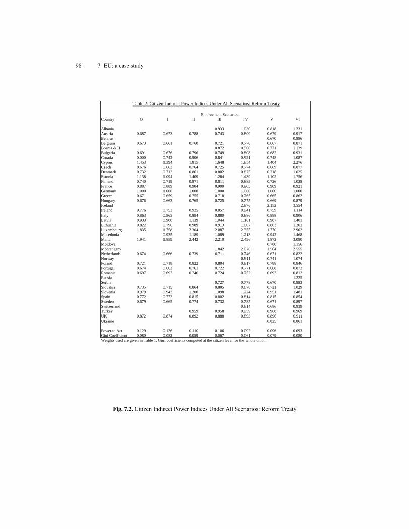
98 7 EU: a case study
Country O I II III IV V VI
Albania 0.933 1.030 0.818 1.231Austria 0.687 0.673 0.788 0.743 0.800 0.679 0.917Belarus 0.670 0.886Belgium 0.673 0.661 0.760 0.721 0.770 0.667 0.871Bosnia & H 0.872 0.960 0.771 1.139Bulgaria 0.691 0.676 0.796 0.749 0.808 0.682 0.931Croatia 0.000 0.742 0.906 0.841 0.921 0.748 1.087Cyprus 1.453 1.394 1.815 1.648 1.854 1.404 2.276Czech 0.676 0.663 0.764 0.725 0.774 0.669 0.877Denmark 0.732 0.712 0.861 0.802 0.875 0.718 1.025Estonia 1.138 1.094 1.409 1.284 1.439 1.102 1.756Finland 0.740 0.719 0.871 0.811 0.885 0.726 1.038France 0.887 0.889 0.904 0.900 0.905 0.909 0.921Germany 1.000 1.000 1.000 1.000 1.000 1.000 1.000Greece 0.671 0.659 0.755 0.718 0.765 0.665 0.862Hungary 0.676 0.663 0.765 0.725 0.775 0.669 0.879Iceland 2.876 2.152 3.554Ireland 0.776 0.753 0.925 0.857 0.941 0.759 1.114Italy 0.863 0.865 0.884 0.880 0.886 0.888 0.906Latvia 0.933 0.900 1.139 1.044 1.161 0.907 1.401Lithuania 0.822 0.796 0.989 0.913 1.007 0.803 1.201Luxembourg 1.835 1.758 2.304 2.087 2.355 1.770 2.902Macedonia 0.935 1.189 1.089 1.213 0.942 1.468Malta 1.941 1.859 2.442 2.210 2.496 1.872 3.080Moldova 0.780 1.156Montenegro 1.842 2.076 1.564 2.555Netherlands 0.674 0.666 0.739 0.711 0.746 0.671 0.822Norway 0.911 0.741 1.074Poland 0.721 0.718 0.822 0.804 0.817 0.788 0.846Portugal 0.674 0.662 0.761 0.722 0.771 0.668 0.872Romania 0.697 0.692 0.746 0.724 0.752 0.692 0.812Russia 1.225Serbia 0.727 0.778 0.670 0.883Slovakia 0.735 0.715 0.864 0.805 0.878 0.721 1.029Slovenia 0.979 0.943 1.200 1.098 1.224 0.951 1.481Spain 0.772 0.772 0.815 0.802 0.814 0.815 0.854Sweden 0.679 0.665 0.774 0.732 0.785 0.671 0.897Switzerland 0.814 0.686 0.939Turkey 0.959 0.958 0.959 0.968 0.969UK 0.872 0.874 0.892 0.888 0.893 0.896 0.911Ukraine 0.825 0.861
Power to Act 0.129 0.126 0.110 0.106 0.092 0.096 0.093Gini Coefficient 0.080 0.082 0.059 0.067 0.061 0.079 0.080Weights used are given in Table 1. Gini coefficients computed at the citizen level for the whole union.
Enlargement Scenarios
Table 2: Citizen Indirect Power Indices Under All Scenarios: Reform Treaty
Fig. 7.2. Citizen Indirect Power Indices Under All Scenarios: Reform Treaty

7.5 Analysis: enlargement scenarios 99
O I II III IV V VICountry Weight EU27 EU29 EU30 EU34 EU37 EU40 EU41Albania 1786 1.0004 1.0005 1.0005 0.9987Austria 2875 1.0017 1.0017 1.0006 1.0007 1.0008 1.0007 0.9989Belarus 3113 1.0009 0.9991Belgium 3242 1.0018 1.0019 1.0007 1.0008 1.0009 1.0008 0.9990Bosnia & H 1984 1.0007 1.0007 1.0007 0.9990Bulgaria 2778 1.0015 1.0016 1.0004 1.0006 1.0007 1.0006 0.9988Croatia 2134 1.0014 1.0003 1.0004 1.0005 1.0005 0.9987Cyprus 875 1.0007 1.0007 0.9996 0.9998 0.9999 0.9999 0.9981Czech 3202 1.0019 1.0020 1.0008 1.0009 1.0010 1.0009 0.9991Denmark 2330 1.0016 1.0017 1.0006 1.0007 1.0008 1.0008 0.9990Estonia 1160 1.0015 1.0017 1.0004 1.0007 1.0008 1.0008 0.9990Finland 2293 1.0016 1.0018 1.0007 1.0008 1.0009 1.0008 0.9991France 7937 1.0025 1.0025 1.0015 1.0014 1.0014 1.0011 1.0001Germany 9080 1.0000 1.0000 1.0000 1.0000 1.0000 1.0000 1.0000Greece 3335 1.0018 1.0018 1.0006 1.0007 1.0008 1.0007 0.9989Hungary 3174 1.0016 1.0018 1.0006 1.0007 1.0008 1.0007 0.9989Iceland 549 1.0011 1.0011 0.9993Ireland 2052 1.0015 1.0017 1.0006 1.0007 1.0008 1.0008 0.9990Italy 7665 1.0028 1.0028 1.0016 1.0016 1.0015 1.0013 1.0002Latvia 1515 1.0014 1.0015 1.0004 1.0006 1.0006 1.0006 0.9989Lithaunia 1845 1.0014 1.0016 1.0004 1.0006 1.0006 1.0006 0.9989Luxembourg 678 1.0015 1.0013 1.0011 1.0005 1.0006 1.0006 0.9988Macedonia 1428 1.0014 1.0006 1.0007 1.0008 1.0008 0.9990Malta 636 1.0013 1.0013 1.0011 1.0005 1.0005 1.0006 0.9989Moldova 1948 1.0006 0.9989Montenegro 773 0.9999 1.0000 1.0000 0.9982Netherlands 4042 1.0023 1.0024 1.0012 1.0012 1.0012 1.0011 0.9994Norway 2167 1.0004 1.0004 0.9986Poland 6177 1.0030 1.0030 1.0017 1.0017 1.0017 1.0014 0.9999Portugal 3251 1.0018 1.0019 1.0007 1.0008 1.0009 1.0008 0.9990Romania 4649 1.0026 1.0027 1.0013 1.0014 1.0014 1.0012 0.9995Russia 11937 0.9943Serbia 3140 1.0009 1.0010 1.0009 0.9991Slovakia 2321 1.0013 1.0014 1.0003 1.0004 1.0005 1.0004 0.9986Slovenia 1415 1.0007 1.0011 1.0000 1.0001 1.0002 1.0002 0.9984Spain 6615 1.0031 1.0031 1.0018 1.0018 1.0018 1.0015 1.0000Sweden 3008 1.0018 1.0018 1.0007 1.0008 1.0009 1.0008 0.9990Switzerland 2736 1.0009 1.0008 0.9990Turkey 8653 1.0007 1.0007 1.0007 1.0005 1.0001UK 7771 1.0027 1.0026 1.0015 1.0015 1.0014 1.0012 1.0001Ukraine 6797 1.0014 1.0000
Total 95921 99483 108136 115,819 121271 133129 145066Quota: 59062 60917 66052 70076 72929 79451 86735
Power indices computed using program ipgenf from website, Leech and Leech (2004).
Table 3: Citizen Indirect Power Indices Under All Scenarios: Jagiellonian Compromise
Enlargement Scenarios
Fig. 7.3. Citizen Indirect Power Indices Under All Scenarios: Jagiellonian Compromise

100 7 EU: a case study
7.6 Conclusions
We have tested the suitability of the proposed Double Majority rule in the EUReform Treaty by looking at its implications for voting power under various en-largement scenarios, some of which are realistic prospects, while some are nomore than speculations. Our scenarios include the possibility of virtually all Eu-ropean countries, up to and even including Russia, acceding to membership. Wehave also tested the performance of the Jagiellonian compromise based on thePenrose Square Root rule whereby voting weights are determined by a simpleformula as proportional to population square roots. In judging the voting rule welooked at two criteria: (i) equality of voting power as measured by the Penrosepower index at the level of the citizen, assuming one-person-one-vote in nationalelections, and (ii) decisiveness of the Council of Ministers, as measured by theColeman power to act. We found that for the present union of 27, the ReformTreaty voting rule gives a much more unequal distribution of citizen voting powerthan the existing voting rule, although it leads to the Council of Ministers beingmore decisive. The Jagiellonian compromise leads to the equalisation of citizenvoting power in all countries.
In considering enlargement scenarios, the inequality of citizen voting powerpersists with each enlargement. The common pattern is for citizens of the small-est countries to have the greatest voting power, sometimes by a factor of as muchas 2 or 3 times those of other countries, such as in the cases of Malta and Luxem-bourg. The medium sized countries have the smallest citizen voting power. Thatfor Netherlands, for example, varies from about two-thirds that of Germany inEU27 to about four fifths of it following the accession of Russia. Our conclusionis that the Reform Treaty voting system is a flawed proposal that fails to reachthe democratic ideal of equality of voting power of all citizens in the EuropeanUnion. This ideal is reached by the Jagiellonian Compromise.
On a more general note, some experiments were also conducted to see if thereis critical quota for which the Shapley-Shubik indices are proportional to theweights. The weights are integers randomly generated from a uniform distribution

7.6 Conclusions 101
on [1, 100] with 30, 40 and 50 players. However, no sharp threshold was observedwhere the weights are proportional to the Shapley-Shubik indices.
Figure 1 Relative Citizen Power: Large Countries
0.700
0.750
0.800
0.850
0.900
0.950
1.000
O I II III IV V VI
Scenario
FranceGermanyItalyPolandSpainUK
Fig. 7.4. Relative Citizen Power: Large Countries
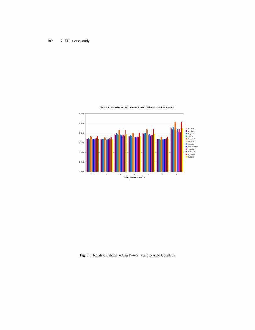
102 7 EU: a case study
Figure 2: Relative Citizen Voting Power: Middle-sized Countries
0.000
0.200
0.400
0.600
0.800
1.000
1.200
O I II III IV V VI
Enlargement Scenario
AustriaBelgiumBulgariaCzechDenmarkGreeceHungaryNetherlandsPortugalRomaniaSlovakiaSweden
Fig. 7.5. Relative Citizen Voting Power: Middle-sized Countries
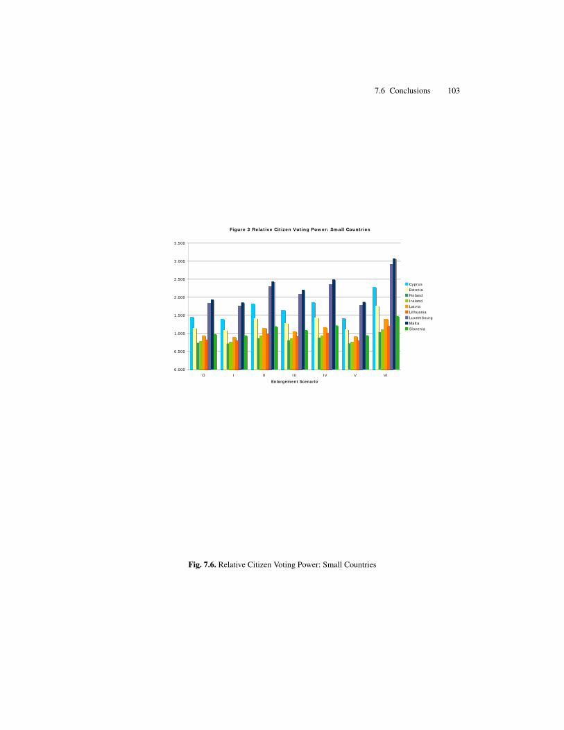
7.6 Conclusions 103
Figure 3 Relative Citizen Voting Power: Small Countries
0.000
0.500
1.000
1.500
2.000
2.500
3.000
3.500
O I II III IV V VI
Enlargement Scenario
CyprusEstoniaFinlandIrelandLatviaLithuaniaLuxembourgMaltaSlovenia
Fig. 7.6. Relative Citizen Voting Power: Small Countries


Part III
Complexity of manipulation

8
Complexity of control in weighted voting games
Complexity is not always a disease to be diagnosed; sometimes it is a
resource to be exploited. But complexity turns out to be most elusive where
it would be most welcome.
- Christos Papadimitriou
Would it then be possible to construct a hierarchy reflecting the difficulty
of benefiting from strategic behavior?
- Hannu Nurmi [160]
Abstract An important aspect of mechanism design in social choice protocolsand multiagent systems is to discourage insincere behaviour. Manipulative be-haviour has received increased attention since the famous Gibbard-Satterthwaitetheorem. We examine the computational complexity of manipulation in weightedvoting games which are ubiquitous mathematical models used in economics, po-litical science, neuroscience, threshold logic, reliability theory and distributedsystems. It is a natural question to check how changes in weighted voting gamemay affect the overall game. Tolerance and amplitude of a weighted voting gamesignify the possible variations in a weighted voting game which still keep thegame unchanged. We characterize the complexity of computing the tolerance andamplitude of weighted voting games. Tighter bounds and results for the toleranceand amplitude of key weighted voting games are also provided.

108 8 Complexity of control in weighted voting games
8.1 Introduction
In this section a general motivation to consider manipulation in WVGs is pre-sented. WVGs have received increased interest in the artificial intelligence andagents community due to their ability to model various coalition formation sce-narios [69]. Such games have also been examined from the point of view of sus-ceptibility to manipulations [21, 220]. WVGs have been applied in various politi-cal and economic organizations [134, 130, 1]. Voting power is used in joint stockcompanies where each shareholder gets votes in proportion to the ownership of astock [94].
WVGs and coalitional voting games are also encountered in threshold logic,reliability theory, neuroscience and logical computing devices [202, 208, 184].There are many parallels between reliability theory and voting theory [184].Parhami [171] points out that voting has a long history in reliability systemsdating back to von Neumann [212]. Nordmann et al. [159] deal with reliabil-ity and cost evaluation of weighted dynamic-threshold voting-systems. Systemsof this type are used in various areas such as target and pattern recognition, safetymonitoring and human organization systems.
Elkind et al. [69] note that since WVGs have only two possible outcomes,they do not fall prey to manipulation of the type characterized by Gibbard-Satterthwaite [97]. The Gibbard-Satterthwaite theorem basically says that anyreasonable voting system with three or more candidates is vulnerable to tacticalvoting. However, there are various ways WVGs can be manipulated and con-trolled. We examine some of the aspects. Tolerance and amplitude of WVGs sig-nify the possible variances in a WVG which still keep the game unchanged. Theyare significant in mathematical models of reliability systems and shareholdings.For reliability systems, the weights of a WVG can represent the significance ofthe components, whereas the quota can represent the threshold for the overallsystem to fail. It is then a natural requirement to provide a framework which canhelp identify similar reliability systems. In shareholding scenarios [5], there is aneed to check the maximum changes in shares which still maintain the status quo.In political settings, the amplitude of a WVG signifies the maximum percentage
8.2 Tolerance & amplitude: background 109
change in various votes which is possible without changing the voting powers ofthe voters. In this chapter, the computational aspects of amplitude and toleranceof WVGs are examined.
Section 8.2 provides a background of tolerance and amplitude. In Section 8.3,computational aspects of tolerance and amplitude are examined. It is seen thatcomputing the amplitude and tolerance of a WVG is NP-hard. We give tighterbounds and results for the tolerance and amplitude of key WVGs such as uniform(symmetric) WVGs and unanimity WVGs.
The final section presents conclusions and ideas for future work.
8.2 Tolerance & amplitude: background
If the valuation function of a WVG v is same as another WVG v′, then v′ is calleda representation of v. If the quota q′ of v′ is such that for all S ⊆ N,
∑i∈S wi
′ , q′,then v′ is called a strict representation of v [89].
8.2.1 Background
The question we are interested in is to find the maximum possible variationsin the weights and quotas of a WVG which still do not change the game. Thetwo key references which address this question are [109] and [89]. Hu [109]worked within the theory of switching functions. He set forth the idea of linearly
separable switching functions which are equivalent to each other. Freixas andPuente [89] extended the theory by framing it in the context of strict representa-tions of WVGs, which are equivalent to linearly separable switching functions.
8.2.2 Tolerance
The setting of the problem is that we look at a transformation, f(λ1,...,λn),Λ whichmaps a WVG, v = [q; w1, . . . ,wn] to v′ = [q′; w1
′, . . . ,wn′] such that wi
′ = (1 +
λi)wi and q′ = (1 + Λ)q. Let A be the maximum of w(S ) for all {S |v(S ) = 0}.and let B be the minimum of w(S ) for all {S |v(S ) = 1}. Then A < q ≤ B (andq < B if the representation is strict). Moreover, let m = Min(q − A, B − q) and
110 8 Complexity of control in weighted voting games
M = q + w(N). Hu [109] and then Freixas and Puente [89] showed that if for all1 ≤ i ≤ n, |λi| < m/M and |Λ| < m/M, then v′ is just another representation ofv. They defined τ[q; w1, . . . ,wn] = m/M as the tolerance of the system. Freixasand Puente [89] also showed that the tolerance is less than or equal to 1/3 forstrict representations of a WVG and less than or equal to 1/5 for a not necessarilymonotonic1 WVG.
8.2.3 Amplitude
Freixas and Puente defined the amplitude as the maximum µ such that f(λ1,...,λn),Λ
is a representation of v whenever Max(|λ1|, . . . , |λn|, |Λ|) < µ(v). For a strict repre-sentation of a WVG [q; w1, . . . ,wn], for each coalition S ⊆ N, let a(S ) = |w(S )−q|
and b(S ) = q + w(S ).Freixas and Puente [89] showed that the amplitude of a WVG is µ(v) =
InfS⊆N
a(S )b(S ) . Although both tolerance and amplitude have been used in the WVG lit-
erature to signify the maximum possible variation in the weights and the quotawithout changing the game, the amplitude is a more precise and accurate indica-tor of the maximum possible variation than tolerance.
8.3 Tolerance & amplitude: some results
8.3.1 Complexity
In all the complexity proofs in this section, we assume that the weights in a WVGare positive integers. We let WVG-STRICT be the problem of checking whethera WVG v = [q; w1, . . . ,wn] is strict or not, i.e., WVG-STRICT = {v: v is strict}.Then we have the following proposition:
Proposition 8.1. WVG-STRICT is co-NP-complete.
Proof. Let WVG-NOT-STRICT = {v: v is not strict}. WVG-NOT-STRICT is inNP since a certificate of weights can be added in linear time to confirm that they
1 Freixas and Puente also consider WVGs where players’ weights can be negative.

8.3 Tolerance & amplitude: some results 111
sum up to q. Moreover v is not strict if and only if there is a subset of weightswhich sum up to q. Therefore the NP-complete problem SUBSET-SUM (seeGarey and Johnson [95]) reduces to WVG-NOT-STRICT. Hence WVG-NOT-STRICT is NP-complete and WVG-STRICT is co-NP-complete. ut
Corollary 8.2. The problem of checking whether the amplitude of a strict WVG
is zero is NP-hard.
Proposition 8.3. The problem of computing the amplitude of a WVG v is NP-
hard.
Proof. Let us assume that weights in v are even integers whereas the quota q isan odd integer 2k − 1. Then the minimum possible difference between q and A,the weight of the maximal losing coalition, or q and B, the weight of minimalwinning coalition is 1. So A ≤ 2k − 2 and B ≥ 2k. We see that µ(v) ≤ 1/(4k − 1)if and only if there exists a coalition C such that w(C) = 2k. Thus the problem ofcomputing µ(v) for a WVG is NP-hard by a reduction from the SUBSET-SUMproblem. ut
A similar proof can be used to prove the following proposition:
Proposition 8.4. The problem of computing the tolerance of a strict WVG is NP-
hard.
8.3.2 Uniform and unanimity WVGs
We show that the bound for the maximum possible tolerance can be improvedwhen we restrict to strict representations of special cases of WVGs. We first lookat uniform WVGs which are an important subclass of WVGs which model manymulti-agent scenarios where each agent has the same voting power.
Proposition 8.5. For a strict representation of a proper uniform WVG v =
[q; w, . . . ,w︸ ︷︷ ︸n
], τ(v) ≤ 13n .

112 8 Complexity of control in weighted voting games
Proof. Since q−Aq+w(N) = 1 − w(N)+A
q+w(N) is an increasing function of q and B−qq+w(N) is
a decreasing function of q, the tolerance reaches its maximum when q − A =
B − q, i.e. when q is the arithmetic mean A+B2 . We let the size of the maximal
losing coalition be r and the size of the minimal winning coalition be r + 1. Thenthe weight of a maximal losing coalition is rw and the weight of the minimalwinning coalition is (r + 1)w and m = w/2. Since v is proper, q ≥ 1
2 (nw), andM = q + w(N) ≥ 3nw
2 . Then,
τ(v) = m/M ≤1
3n.
ut
Proposition 8.6. For a uniform WVG v = [q; w, . . . ,w︸ ︷︷ ︸n
], we have B = wd qwe and
A = B − w. Then,
µ(v) =
q−AA+q , if q ≤
√AB
B−qB+q , otherwise.
Proof. It is clear that B, the weight of the minimal winning coalition is wd qwe and
A, the weight of the maximal losing coalition is B−w. Note that, q−Aq+A ≤
B−qq+B if and
only if q ≤√
AB. For losing coalitions with weight w, q−wq+w is a decreasing function
for w. For winning coalitions with weight w, w−qq+w = 1 − 2q
q+w is an increasingfunction for w. Thus if q ≤
√AB, µ(v) =
q−AA+q . Otherwise, µ(v) =
B−qB+q . ut
Corollary 8.7. The amplitude µ(v) of a uniform WVG v can be found in O(1), i.e.,
constant, time.
Proof. The corollary immediately follows from the previous theorem. ut
We now look at unanimity WVGs, which are another important subclass ofWVGs in which a coalition is winning if and only if it is the grand coalitionN.
Proposition 8.8. For a unanimity WVG v = [q; w1, . . . ,wn],
τ(v) ≤wn
4w(N) − wn≤
14n − 1
.

8.4 Conclusion and future work 113
Proof. We know that B = w(N) and A = w(N)−wn, which means that w(N)−wn <
q ≤ w(N). For maximum tolerance, q = A+B2 = w(N) − wn
2 . Therefore m = wn/2and M = w(N) − wn
2 + w(N). Then the tolerance of v satisfies:
τ(v) ≤mM
=wn
4w(N) − wn≤
14n − 1
,
since wn ≤ w(N)/n. ut
Note that we do not insist that wti ≥ wt
j for all i < j and 1 ≤ t ≤ m. Let(N, v) = (N, v1 ∧ ... ∧ vm) be a multiple weighted voting game. Then we cansee that µ(v) ≥ Inf(µ(v1), . . . , µ(vm)). The reason is that for v to change, at leastone constituent game has to change. However it is not necessary that a changein any one game vi changes v. As a simple example, suppose v1 = [2; 2, 1] andv2 = [2; 1, 2]. Then µ(v1∧v2) = 1/5, as witnessed by the coalition {1, 2}. However,µ(vi) = 0, as witnessed by {i}, for i = 1, 2.
8.4 Conclusion and future work
We have examined the computational complexity of computing the toleranceand amplitude of WVGs. The tolerance and amplitude of uniform and unanim-ity games is also analysed. There is a need to devise approximation algorithmsfor computing the amplitude of a WVG. The analysis of amplitude and toler-ance motivates the formulation of an overall framework to check the ‘sensitivity’of voting games under fluctuations and susceptibility to control. It will be inter-esting to explore the limit of changes in WVGs in alternative representations ofsimple games.


9
False-name manipulations
...some voting procedures can be inherently resistant to abuse, while oth-
ers are vulnerable. We base this distinction on a measure that is new to
voting theory - computational complexity.
- Bartholdi, Tovey and Trick [114]
Life is not long, and too much of it should not be spent in idle deliberation.
- Samuel Johnson
Abstract We examine the computational complexity of false-name manipulationin weighted voting games. Weighted voting games have received increased inter-est in the multiagent community due to their compact representation and abilityto model coalitional formation scenarios. Bachrach and Elkind in their AAMAS2008 paper examined divide and conquer false-name manipulation in weightedvoting games from the point of view of Shapley-Shubik index. We analyse thecorresponding case of Banzhaf index and check how much the Banzhaf index of aplayer increases or decreases if it splits up into sub-players. A pseudo-polynomialalgorithm to find the optimal split is also provided. Bachrach and Elkind alsomentioned manipulation via merging as an open problem. In the chapter, we ex-amine the cases where a player annexes other players or merges with them to in-crease their Banzhaf index or Shapley-Shubik index payoff. We characterize thecomputational complexity of such manipulations as well as providing limits tothe manipulation. The Annexation Non-monotonicity paradox is also discovered

116 9 False-name manipulations
in the case of the Banzhaf index. The results give insight into coalition formationand manipulation.
9.1 Introduction
There are various ways WVGs can be manipulated and controlled. Splitting ofa player into sub-players can be seen as a false-name manipulation by an agentwhere it splits itself into multiple agents so that the sum of the utilities of thesplit-up players is more than the utility of the original player [21]. We examinesituations when splitting up into smaller players may be advantageous or disad-vantageous to a player in the context of WVGs and Banzhaf indices. This gives abetter idea of how to devise WVGs in which manipulation can be deterred. Thismay be done by keeping larger or non-integer weights. Moreover, we also exam-ine the case of players merging to maximize their payoff in a WVG. This wasmentioned as an unexplored question in [21].
The outline of the chapter is as following. Section 9.2 provides a brief liter-ature survey. In Section 9.3, the case of players splitting up into sub-players ina WVG to increase their Banzhaf index is analysed. We examine the extent towhich the Banzhaf index of a player can increase or decrease if it splits up intosub-players. From a computational perspective, it is #P-hard [179] to computethe payoff in the WVG. A prospective manipulator could still be interested in en-abling a beneficial split even if he cannot compute the actual payoff. Moreover,this model is reasonable because the central authority which organizes the gameis assumed to have much more computational resource than the players. In Sec-tion 9.4, we prove that it is NP-hard even to decide whether a split is beneficialor not. In the end a pseudo-polynomial algorithm is proposed which returns ‘no’if no beneficial split is available and returns the optimal split otherwise. Section9.5 is about the case of players annexing others or voluntarily merging into blocsto maximize their payoffs. It is shown that for both the Banzhaf index and theShapley-Shubik index, it is NP-hard to find a beneficial merge and for the caseof the Banzhaf index, it is NP-hard to decide a beneficial annexation. Limits to

9.3 Splitting 117
manipulation are also provided. The final section presents conclusions and ideasfor future work.
9.2 Related work
WVGs have also been examined from the point of view of control and manip-ulation. Zuckerman et al. [220] analyse how the centre might control WVGsby changing the quota even if the weights are fixed. The most relevant workis by Bachrach and Elkind [21] where they examine false-name manipulation inWVGs from the point of view of the Shapley-Shubik index. In fact, this chapteranswers problems posed by Bachrach and Elkind. Players forming blocs havebeen considered by political scientists and economists previously [82]. How-ever, in this chapter, a complexity theoretic analysis of bloc forming manipulationhas also been undertaken for WVGs. False name manipulations in open anony-mous environments have been examined in different domains such as coalitionalgames [219, 162, 161] and auctions [218, 113]. The characteristic function byitself does not give enough information to analyze false-name manipulations es-pecially if a player splits into sub-players. Therefore Yokoo et al. [219] introducedthe model where each player has a subset of skills and the characteristic functionassigns values to the subset of skills. We notice that false-name manipulationsin WVGs can still be analyzed directly without considering more fine-grainedrepresentations.
9.3 Splitting
In the real world, WVGs may be dynamic. Players might have an incentive tosplit up into smaller players or merge into voting blocs. Payoffs of players in acoalitional games setting can be based on fairness, i.e., power indices, or theycan be based on the notion of stability, which includes many cooperative gametheoretic concepts such as core, nucleolus etc. We examine the situation when theBanzhaf indices of agents can be used as payoffs in a cooperative game theoretic
118 9 False-name manipulations
situation. Falsenthal and Machover [146] refer to this notion of voting power asP-power since the motivation of agents is prize-seeking as opposed to influence-seeking. However Banzhaf indices have been considered as possible payments incooperative settings [211, 21] and they satisfy desirable axioms [63]. Splitting ofa player can be seen as a false-name manipulation by an agent, in which it splitsitself into multiple agents so that the sum of the utilities of the split-up players ismore than the utility of the original player [21].
Splitting is not always beneficial. We give examples where, if we use Banzhafindices as payoffs of players in a WVG, splitting can be advantageous, neutral ordisadvantageous.
Example 9.1. Splitting can be advantageous, neutral or disadvantageous:
• Disadvantageous splitting. In the WVG [5; 2, 2, 2] each player has a Banzhafindex of 1/3. If the last player splits up into two players, the new game is[5; 2, 2, 1, 1]. In that case, the split-up players have a Banzhaf index of 1/8each.
• Neutral splitting. In the WVG [4; 2, 2, 2] each player has a Banzhaf index of1/3. If the last player splits up into two players, the new game is [4; 2, 2, 1, 1].In that case, the split-up players have a Banzhaf index of 1/6 each.
• Advantageous splitting. In the WVG [6; 2, 2, 2] each player has a Banzhafindex of 1/3. If the last player splits up into two players, the new game is[6; 2, 2, 1, 1]. In that case, the split-up players have a Banzhaf index of 1/4each.
We analyse the splitting of players in the unanimity WVG.
Proposition 9.2. In a unanimity WVG with q = w(N), if Banzhaf indices are used
as payoffs of agents in a WVG, then it is beneficial for an agent to split up into
several agents.
Proof. In a WVG with q = w(N), the Banzhaf index of each player is 1/n. Letplayer i split up into m + 1 players. In that case there is a total of n + m playersand the Banzhaf index of each player is 1/(n + m). In that case the total Banzhafindex of the split up players is m+1
n+m , and for n > 1, m+1n+m > 1
n . ut
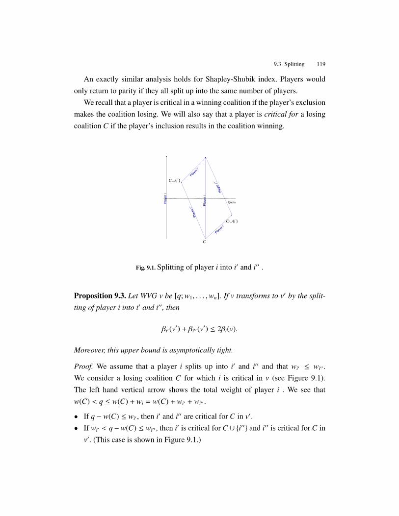
9.3 Splitting 119
An exactly similar analysis holds for Shapley-Shubik index. Players wouldonly return to parity if they all split up into the same number of players.
We recall that a player is critical in a winning coalition if the player’s exclusionmakes the coalition losing. We will also say that a player is critical for a losingcoalition C if the player’s inclusion results in the coalition winning.
C
}{ 'iC∪
}{ ''iC∪
Fig. 9.1. Splitting of player i into i′ and i′′ .
Proposition 9.3. Let WVG v be [q; w1, . . . ,wn]. If v transforms to v′ by the split-
ting of player i into i′ and i′′, then
βi′(v′) + βi′′(v′) ≤ 2βi(v).
Moreover, this upper bound is asymptotically tight.
Proof. We assume that a player i splits up into i′ and i′′ and that wi′ ≤ wi′′ .We consider a losing coalition C for which i is critical in v (see Figure 9.1).The left hand vertical arrow shows the total weight of player i . We see thatw(C) < q ≤ w(C) + wi = w(C) + wi′ + wi′′ .
• If q − w(C) ≤ wi′ , then i′ and i′′ are critical for C in v′.• If wi′ < q −w(C) ≤ wi′′ , then i′ is critical for C ∪ {i′′} and i′′ is critical for C in
v′. (This case is shown in Figure 9.1.)

120 9 False-name manipulations
• If q −w(C) > wi′′ , then i′ is critical for C ∪ {i′′} and i′′ is critical for C ∪ {i′} inv′.
We see that for any swing for player i, there are is an addition of exactly twoswings for the players i′ and i′′. Also if i is not critical for coalition, then neithercan i′ and i be critical for that coalition. Therefore we have ηi′(v′)+ηi′′(v′) = 2ηi(v)in each case.
Now we consider a player x in v which is other than player i. If x is criticalfor a coalition C in v then x is also critical for the corresponding coalition C′ inv′ where we replace {i} by {i′, i′′}. Hence ηx(v) ≤ ηx(v′). Of course x may also becritical for some coalitions in v′ which contain just one of i′ and i′′, so the aboveinequality will not in general be an equality. Moreover,
βi′(v′) + βi′′(v′) =2ηi(v)
2ηi(v) +∑
x∈N(v′)\{i′,i′′} ηx(v′)
≤2ηi(v)
2ηi(v) +∑
x∈N(v)\{i} ηx(v)
≤2ηi(v)
ηi(v) +∑
x∈N(v)\{i} ηx(v)= 2βi(v)
We can prove that this coefficient of 2 is best possible asymptotically. We takea WVG [n; 2, 1, . . . , 1] with n + 1 players. We find that η1 = n +
(n2
)and for all
other x, ηx = 1 +(
n−12
). Therefore
β1 =n +
(n2
)n +
(n2
)+ n(1 +
(n−1
2
))
=n + 1
(n − 2)2 ∼ 1/n.
In case player 1 splits up into 1′ and 1′′ with weights 1 each, then for all playersj, β j = 1
n+2 . Thus for large n, β1′ + β1′′ = 2n+2 ∼ 2β1. ut
It can be shown [67] that in the case of Banzhaf index, the disadvantage insplitting into two players cannot be more than by a factor of 1/(n + 1):
Proposition 9.4. Let WVG v be [q; w1, . . . ,wn]. If v transforms to v′ by the split-
ting of player i into i′ and i′′, then βi′(v′) + βi′′(v′) ≥βi(v)n+1 .

9.3 Splitting 121
Proof. Consider S ⊆ N \ {i, x}. If player x distinct from i is critical for S , then inthe extreme case it may possibly be critical for S , S ∪{i′}, S ∪{i′′} and S ∪{i′, i′′}.Assume that x is not critical for S but x is critical for S ∪ {i′}. This implies thatv′(S ) = 0, v′(S ∪{x}) = 0 and v′(S ∪{x, i′}) = 1 which means that i′ is also criticalfor S ∪ {x}. Then, new coalitions of the form S ∪ {i′} or S ∪ {i′′} produced forwhich x is critical cannot be more than η′i(v
′) + η′′i (v′) = 2ηi(v). Then we have,
βi′(v′) + βi′′(v′) =2ηi(v)
2ηi(v) +∑
x∈N(v′)\{i′,i′′} ηx(v′)
≥2ηi(v)
2ηi(v) + 4∑
x∈N(v)\{i} ηx(v) + 2(n)ηi(v)
≥2ηi(v)
2ηi(v) + 2(n + 1)∑
x∈N(v)\{i} ηx(v) + 2(n)ηi(v)
=βi(v)n + 1
ut
It is believed that the lower bound proved in Proposition 9.4 is not tight. Wenow show that splitting into two players can decrease the Banzhaf index payoff
by as much as a factor of almost√
π2n :
Example 9.5. Disadvantageous splitting. We take a WVG v on n players wherev = [3n/2; 2n, 1, . . . , 1]. For the sake of simplicity, we assume that n is even. It iseasy to see that player 1 is a dictator. Now we consider the case where v changesinto v′ with player 1 splitting up into 1′ and 1′′ with weight n each. For player1′ to be critical for a losing coalition in v′, the coalition much exclude 1′′ andhave from n/2 to n− 1 players with weight 1 or it must include 1′′ and have from0 to (n/2 − 1) players with weight 1. So η1′(v′) = η1′′(v′) =
∑ni=0
(n−1
i
)= 2n−1.
Moreover, for a smaller player x with weight 1 to be critical for a coalition inv′, the coalition must include only one of 1′ or 1′′ and (n − 2)/2 of the n − 2

122 9 False-name manipulations
other smaller players. So, ηx(v′) = 2(
n−2(n−2)/2
). By using Stirling’s formula, we can
approximate ηx(v′) by√
2π(n−2)2
n−1. We see that:
βi′(v′) = βi′′(v′)
≈2n−1
2n−1 + 2n−1 + (n − 1)√
2π(n−2)2
n−1
=1
2 +(n−1)√
n−2
√2π
∼
√π
2n.
We notice that the bounds on the effect of splitting on the Banzhaf index arequite similar to those in the Shapley-Shubik case (see Table 9.2).
9.4 Complexity of finding a beneficial split
From a computational perspective, it is #P-hard for a manipulator to find the idealsplitting to maximize his payoff. This is because even computing Banzhaf valuesonce for a WVG is #P-complete.
An easier question is to check whether a beneficial split exists or not. We de-fine a Banzhaf version of the BENEFICIAL SPLIT problem defined in [21].
Name: BENEFICIAL-BZ-SPLITInstance: (v, i) where v is the WVG v = [q; w1, . . . ,wn] and player i ∈ {1, . . . , n}.Question: Is there a way for player i to split his weight wi between sub-playersi1, . . . , im so that, in the new game v′,
∑mj=1 βi j(v
′) > βi(v)?
Proposition 9.6. BENEFICIAL-BZ-SPLIT is NP-hard, and remains NP-hard even
if the player can only split into two players with equal weights.

9.4 Complexity of finding a beneficial split 123
Proof. We prove this by a reduction from an instance of the classical NP-hardPARTITION problem to BENEFICIAL-BZ-SPLIT.
Given an instance of PARTITION {a1, . . . , ak}, we can transform it to a WVGv = [q; w1, . . . ,wn] with n = k + 1 where wi = 8ai for i = 1 to n − 1, wn = 2and q = 4
∑ki=1 ai + 2. After that, we want to see whether it can be beneficial for
player n with weight 2 to split into two sub-players n and n + 1 each with weight1 to form a new WVG v′ = [q; w1, . . . ,wn−1, 1, 1]. Note that, since the weights areintegral, it is certainly not possible to split up a weight of 2 other than into 1 and1.
If A is a ‘no’ instance of PARTITION, then we see that no subset of the weights{w1, . . . ,wn−1} can sum to 4
∑i ai. This implies that player n is a dummy. We see
that even if player n splits into sub-players, the sub-players are also dummies.Therefore (v, n) is a ‘no’ instance of BENEFICIAL-BZ-SPLIT.
Now let us assume that A is a ‘yes’ instance of PARTITION. In that case, letthe number of subsets of weights {w1, . . .wn−1} summing to 4
∑i ai be x. Then
ηn(v) = x. For i ≤ n − 1, player i can be critical in winning coalition with weightexactly q or more than q. We note that exactly half of the x subsets of {w1, . . .wn−1}
summing to 4∑
i ai contain wi. If player i is critical in a coalition C which is asubset of {w1, . . .wn−1} then i is also critical in C ∪ {wn}. Therefore for i ≤ n − 1,ηi(v) = x
2 + 2yi where yi is the number of subsets of {w1, . . .wn−1} in which i iscritical. We see that
βn(v) =x
x + kx2 + 2y
where∑
i≤n−1
yi = y.
However, in the new game v′, ηn(v′) = ηn+1(v′) = x and for i ≤ n − 1, ηi(v′) =x2 + 4yi, since there are now 4 coalitions, C,C ∪ {wn},C ∪ {wn+1},C ∪ {wn,wn+1},corresponding to each C. So
βn(v′) + βn+1(v′) =2x
2x + kx/2 + 4y> βn(v),

124 9 False-name manipulations
since x > 0. Thus, a ‘yes’ instance of PARTITION implies a ‘yes’ instance ofBENEFICIAL-BZ-SPLIT. ut
In terms of minimizing chances of manipulation, we see that computationalcomplexity acts as a barrier. This idea of using computational complexity tomodel bounded rationality is well explained by Papadimitriou and Yannakakis[170]. In the context of complexity of voting, it was a series of groundbreakingpapers by Bartholdi, Orlin, Tovey, and Trick [32, 111, 112, 114] that showedhow important computationally complexity consideration is in terms of ease ofcomputing winners and difficulty of manipulation.
9.4.1 Pseudo-polynomial algorithm
It is well known that, although computing Banzhaf indices of players in aWVG is NP-hard, there are polynomial time algorithms using dynamic pro-gramming [151] or generating functions [36] to compute Banzhaf indices if theweights of players are polynomial in n. Let this pseudo-polynomial algorithmbe BanzhafIndex(v, i) which takes a WVG v and an index i as input and returnsβi(v), the Banzhaf index of player i in v. We use a similar argument as in [21] toshow that a polynomial algorithm exists to find a beneficial split if the weights ofplayers are polynomial in n and the player i in question can split into up to a con-stant k number of sub-players with integer weights. Algorithm 11 takes as input aWVG v and player i which can split into a maximum of k number of players. Thealgorithm returns ‘no’ if no beneficial split exists and returns the optimal splitotherwise. Whenever player i in WVG v splits according to a split s, we denotethe new game by vi,s.
Proposition 9.7. Algorithm 11 is polynomial in n if the weights are polynomial
in n.
Proof. Since the weight values are polynomial in n and we consider splits intoa constant number of players, a brute force method is sufficient. We see that thetotal number of splits for player i is equal to q(wi, k) where q(n, k) is the partitionfunction which gives the number of partitions of n with k or fewer addends. It is

9.5 Merging and annexation 125
Algorithm 11 BeneficialSplitInWVGInput: (v, i) where v = [q; w1, . . . ,wn] and i is the player which wants to split intoa maximum of k sub-players.Output: Returns NO if there is no beneficial split. Otherwise returns the optimalsplit (wi1 , . . . ,wik′ ) where k′ ≤ k, and
∑k′j=1 wi j = wi.
1: BeneficialSplitExists = false2: BestSplit = ∅
3: BestSplitValue = −∞
4: βi = BanzhafIndex(v, i)5: for j = 2 to k do6: for Each possible split s where wi = wi1 + . . . + wi j do7: SplitValue =
∑ ja=1 BanzhafIndex(vi,s, ia)
8: if SplitValue > βi then9: BeneficialSplitExists = true
10: if SplitValue > BestSplitValue then11: BestSplit = s12: BestSplitValue = SplitValue13: end if14: end if15: end for16: end for17: if BeneficialSplitExists = false then18: return false19: else20: return BestSplit21: end if
clear that for a constant k, the number of splits of player i is less than (wi)k whichis a polynomial in n. Since the computational complexity for each split is alsoa polynomial in n, therefore Algorithm 11 is polynomial in n if the weights arepolynomial in n. ut
9.5 Merging and annexation
For the case of players merging to gain advantage, we examine two cases. One isannexation where one voter takes the voting weight of other players. The annexa-
126 9 False-name manipulations
tion is advantageous if the payoff of the new merged coalition in the new game isgreater than the payoff of the annexer in the original game. The other case is vol-untary merging where players merge to become a bloc for which their new payoff
is more than the sum of their individual payoffs. For every game (N, v), the resultof the merging of players in coalition S is another game ((N \ S ) ∪ {&S }, v&S ).
We define the problem of checking a beneficial voluntary merge or annexation:
Name: BENEFICIAL-BZ-MERGEInstance: (v, S ) where v is the WVG v = [q; w1, . . . ,wn] and S ⊂ N.Question: Suppose coalition S merges to form a new game ((N \S )∪{&S }, v&S ).Is β&S (v&S ) >
∑i∈S βi(v)?
Name: BENEFICIAL-BZ-ANNEXATIONInstance: (v, S , i) where v is the WVG v = [q; w1, . . . ,wn], i is the ith player in v
and S ⊂ (N \ {i}).Question: If i annexes coalition S to form a new game ((N \ (S ∪ {i})) ∪ {&(S ∪{i})}, v&(S∪{i})), is βi(v&(S∪{i})) > βi(v)?
If Shapley-Shubik indices are used as payoffs in place of Banzhaf indices,then the corresponding problems are defined with BZ replaced by SS so thatBENEFICIAL-SS-MERGE corresponds to BENEFICIAL-BZ-MERGE. Felsen-thal and Machover [82] prove that if a player annexes other players, then it cannotbe the case that the annexation is disadvantageous if the Shapley-Shubik indicesare used as payoffs. We provide a clear and simple proof of this theorem. Letplayer i be critical for a coalition S in WVG v. Then the contribution to φi(v)from this is (|S |−1)!(n−|S |)!
n! . We consider a game v&{i, j} where i annexes j. For every S
for which i is critical in v, the contribution to φ&{i, j}(v&{i, j}) is either (|S |−2)!(n−|S |)!(n−1)! or
(|S |−1)!(n−|S |−1)!(n−1)! . For either case we see that φ&{i, j}(v&{i, j}) > φi(v). However Felsen-
thal and Machover [82] show that, for the case of the Banzhaf index, annexationcould be disadvantageous. They provide a 13-player WVG for which annexation

9.5 Merging and annexation 127
is disadvantageous, which is the simplest example they could find. We provide an8-player WVG where annexation is disadvantageous:
Example 9.8. In WVG [13; 7, 6, 1, 1, 1, 1, 1, 1], player 1 has Banzhaf index 0.48507.If player 1 annexes one of the small players, the new game is [13; 8, 6, 1, 1, 1, 1, 1]and the Banzhaf index becomes 0.47826.
For the case where the merging is voluntary instead of an annexation, for boththe Banzhaf index and Shapley-Shubik index, merging can be advantageous ordisadvantageous. As in the case of splitting, we expect it to be hard to find abeneficial merge:
Proposition 9.9. BENEFICIAL-BZ-MERGE is NP-hard.
Proof. Given an instance of PARTITION {a1, . . . , ak}, we can transform it to aWVG v = [q; w1, . . . ,wn] where n = k + 3, wi = 8ai for i = 1 to n − 3, wn−2 =
wn−1 = wn = 1, and q = 4∑k
i=1 ai + 2.If A is a ‘no’ instance of PARTITION, then we see that a subset of weights
{w1, . . .wn−3} cannot sum to 4∑
i ai. This implies that players (n − 2), (n − 1) andn are dummies. Even if players n and (n − 1) merge together, the new player&{n − 1, n} remains a dummy in the new game v&{n−1,n}.
Now let us assume that A is a ‘yes’ instance of PARTITION. In that case,let the number of subsets of weights {w1, . . .wn−3} summing to 4
∑i ai be x. For
i ≤ n − 3, player i can be critical in winning coalitions with weight q or q + 1or more than q + 1. The number of coalitions for the first two cases are 3x/2 andx/2, respectively, corresponding to the participation of either 2 or 3 of the unitplayers. The third case corresponds to coalitions in which the three unit playersare dummies. Therefore for i ≤ n − 3, ηi = 4x
2 + 8yi where yi is the number ofsubsets of {w1, . . . ,wn−3} in which i is critical. Moreover, ηn−2(v) = ηn−1(v) =
ηn(v) = 2x, since each unit player is critical only when exactly one other of theseis in the coalition. Then
βn(v) =2x
6x + 4kx2 + 8y
, where∑
i≤n−3
yi = y.

128 9 False-name manipulations
In the new game v&{n−1,n}, η&{n−1,n}(v&{n−1,n}) is 2x but ηn−2(v&{n−1,n}) is 0. Fori ≤ n − 3, ηi(v&{n−1,n}) is 2x
2 + 4yi. We see that
β&{n−1,n}(v&{n−1,n}) =2x
2x + 2kx/2 + 4y.
Therefore,β&{n−1,n}(v&{n−1,n}) > βn(v) + βn−1(v),
which means that n and (n − 1) had a beneficial merge. It has been shown thata ‘yes’ instance of PARTITION implies a ‘yes’ instance of BENEFICIAL-BZ-MERGE. ut
Proposition 9.10. BENEFICIAL-BZ-ANNEXATION is NP-hard.
Proof. Given an instance of PARTITION, {a1, . . . , ak}, we can transform it to aWVG v = [q; w1, . . . ,wn] where n = k + 2, wi = 8ai for i = 1 to n − 2, wn−1 = 1,wn = 1 and q = 4
∑ki=1 ai + 2. Just as in Proposition 9.9, we see that a ‘no’
instance of partition implies that wn−1 and wn are dummies even if n annexes(n − 1). However, a ‘yes’ instance of partition implies that player n benefits byannexing player (n − 1). ut
Proposition 9.11. BENEFICIAL-SS-MERGE is NP-hard
Proof. Given an instance of PARTITION {a1, . . . , ak}, we can transform it to aWVG v = [q; w1, . . . ,wn] where n = k + 3, wi = 8ai for i = 1 to n − 2, wn−2 =
wn−1 = wn = 1, and q = 4∑k
i=1 ai + 2.If A is a ‘no’ instance of PARTITION, then we see that a subset of weights
{w1, . . .wn−3} cannot sum to 4∑
i ai. This implies that players (n − 2), (n − 1)and n are dummies. Even if player n and (n − 1) merge together, the new player&{n − 1, n} remains a dummy in the new game v&{n−1,n}.
Now let us assume that A is a ‘yes’ instance of PARTITION. For each partition(P1, P2) where |P1| = p1 and |P2| = p1, we check the number of permutationscorresponding to (P1, P2). In the original game v, the contribution to the Shapley-Shubik payoff for either player n or (n − 1) by the permutations corresponding to(P1, P2) is

9.5 Merging and annexation 129
2(p1 + 1)!(p2 + 1)!n!
=p1!p2!
n!2(p1 + 1)(p2 + 1).
If players n and n − 1 merge into bloc &{n − 1, n}, then the contribution to theShapley-Shubik payoff to bloc &{n − 1, n} by the permutations corresponding to(P1, P2) is
p1!(p2 + 1)! + (p1 + 1)!p2!(n − 1)!
=p1!p2!
n!(n(p1 + 1 + p2 + 1)).
For the merge to be beneficial, it is required that the sum of the Shapley-Shubikindices of (n−1) and n in the original game v is less than the Shapley-Shubik indexof &{n − 1, n} in the game v&{n−1,n}, i.e., 4(p1 + 1)(p2 + 1) < n(p1 + 1 + p2 + 1).Since (p1 + 1) + (p2 + 1) = n − 1, we have
4(p1 + 1)(p2 + 1) ≤ 4(n − 1
2
)2
< n(n − 1) = n(p1 + 1 + p2 + 1),
and so φn−1(v) + φn(v) < φ&{n−1,n}(v&{n−1,n}). ut
We examine the limits of advantage or disadvantage for the case of the annex-ation of another player to increase the Banzhaf index.
Proposition 9.12.βi(v) + β j(v)
2≤ βi(v&({i, j})) ≤ 1.
Proof. Let v be WVG [q; w1, . . . ,wn]. Suppose i annexes or merges with player j
and v′ is v&({i, j}). Then the new game is ((N \ { j}) ∪ {&({i, j})}, v′). From the proofof Proposition 9.3, we see that η&({i, j})(v′) equals 1
2 (βi(v) + β j(v)).Now consider a player x which is other than player i or player j. Let S be
coalition such that S ⊆ N \ {i, j, x}. If x is critical for S in v then x is critical forS in v′. If x is critical for S ∪ {i, j} in v then x is critical for S ∪ &({i, j}) in v′.However, x may also be critical for S ∪ {i} or S ∪ { j} in v. So ηx(v) ≥ ηx(v′). Wesee that:

130 9 False-name manipulations
β&({i, j})(v′) =η&({i, j})(v′)
η&({i, j})(v′) +∑
x∈(N\{i, j}) ηx(v′)
=
12 (ηi(v) + η j(v))
12 (ηi(v) + η j(v)) +
∑x∈(N\{i, j}) ηx(v′)
≥
12 (ηi(v) + η j(v))
ηi(v) + η j(v) +∑
x∈(N\{i, j}) ηx(v)
=12
(βi(v) + β j(v)).
The upper bound is tight and easy to observe. If player i is a dummy and j is adictator then βi(v) = 0 whereas βi(v′) = 1. The upper bound can also be achievedby two big enough players joining forces. ut
We have seen that annexation can be disadvantageous in the case of theBanzhaf index. One would at least expect the Banzhaf index payoff after annexinganother player to be monotone in the power of the annexed player. Surprisingly,this is not the case. Suppose wi ≥ w j ≥ wk in a WVG v. We provide an examplewhere βi,k > βi, j. We call this the annexation non-monotonicity paradox:
Example 9.13. In the WVG [9; 3, 3, 2, 1, 1, 1] we see that player 2 has moreweight than player 3. However if player 1 annexes player 2 to form game[9; 6, 2, 1, 1, 1], its Banzhaf index is 0.4, whereas if player 1 annexes player 3to form game [9; 5, 3, 1, 1, 1], its Banzhaf index is 7/17 ≈ 0.411765.
Proposition 9.14. For any coalition, S ⊂ N \ {i},
φi(v) ≤ φi(v&({i}∪S )) ≤ 1.
Proof. The lower bound follows from the result by Felsenthal and Machover [82]that annexation cannot decrease the Shapley-Shubik index of a player. Moreover,the upper bound is tight and easily attainable if {i} ∪ S is big enough. ut
Proposition 9.15. For the unanimity game, for both the Shapley-Shubik index and
Banzhaf index:
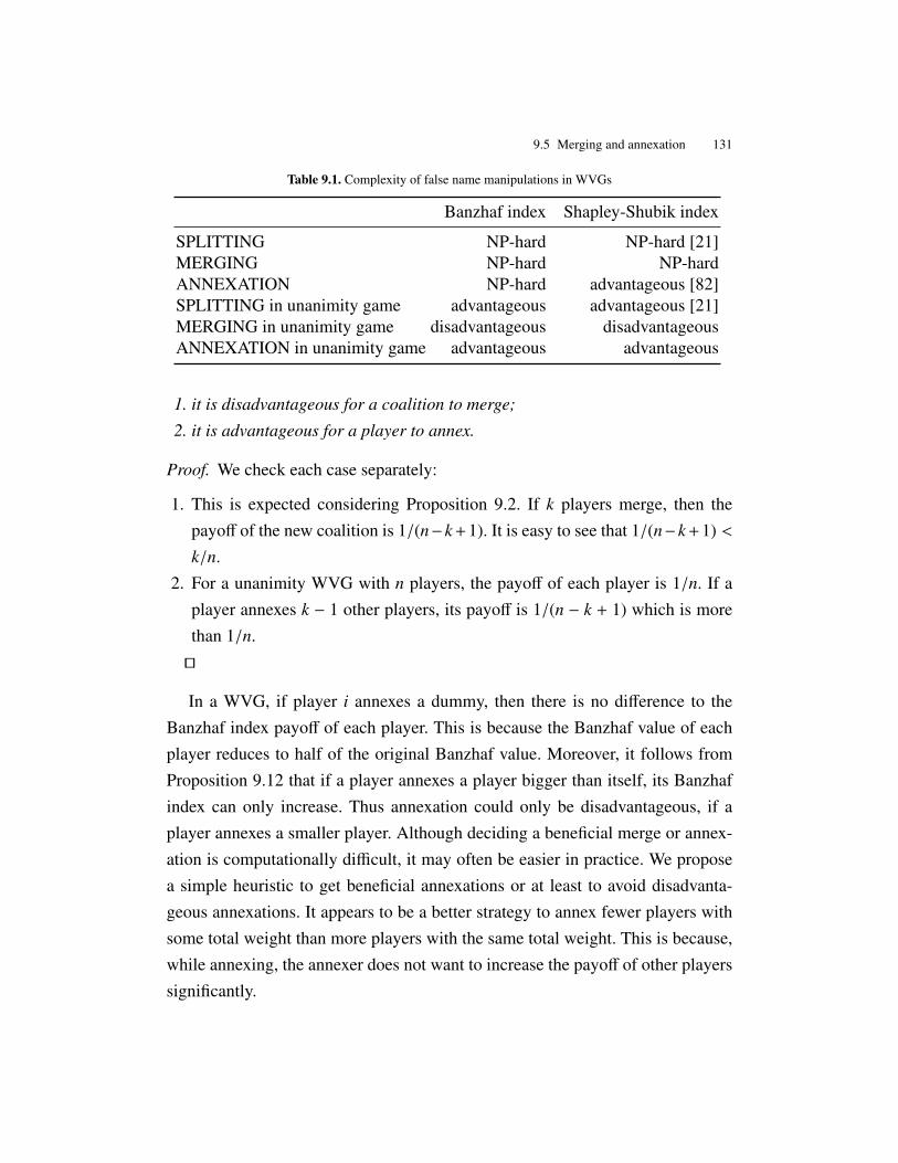
9.5 Merging and annexation 131
Table 9.1. Complexity of false name manipulations in WVGs
Banzhaf index Shapley-Shubik index
SPLITTING NP-hard NP-hard [21]MERGING NP-hard NP-hardANNEXATION NP-hard advantageous [82]SPLITTING in unanimity game advantageous advantageous [21]MERGING in unanimity game disadvantageous disadvantageousANNEXATION in unanimity game advantageous advantageous
1. it is disadvantageous for a coalition to merge;
2. it is advantageous for a player to annex.
Proof. We check each case separately:
1. This is expected considering Proposition 9.2. If k players merge, then thepayoff of the new coalition is 1/(n−k +1). It is easy to see that 1/(n−k +1) <k/n.
2. For a unanimity WVG with n players, the payoff of each player is 1/n. If aplayer annexes k − 1 other players, its payoff is 1/(n − k + 1) which is morethan 1/n.ut
In a WVG, if player i annexes a dummy, then there is no difference to theBanzhaf index payoff of each player. This is because the Banzhaf value of eachplayer reduces to half of the original Banzhaf value. Moreover, it follows fromProposition 9.12 that if a player annexes a player bigger than itself, its Banzhafindex can only increase. Thus annexation could only be disadvantageous, if aplayer annexes a smaller player. Although deciding a beneficial merge or annex-ation is computationally difficult, it may often be easier in practice. We proposea simple heuristic to get beneficial annexations or at least to avoid disadvanta-geous annexations. It appears to be a better strategy to annex fewer players withsome total weight than more players with the same total weight. This is because,while annexing, the annexer does not want to increase the payoff of other playerssignificantly.

132 9 False-name manipulations
Bounds Reference1
n+1βi(v) ≤ βi′(v′) + βi′′(v′) ≤ 2βi(v) Prop 9.4 and 9.3
βi(v)+β j(v)2 ≤ βi(v&({i, j})) ≤ 1. Prop 9.12
φi(v) ≤ φi(v&({i}∪S )) ≤ 1. Prop 9.14
2n+1φi(v) ≤ φi′(v′) + φi′′(v′) ≤ 2n
n+1φi(v) [21]
Table 9.2. Bounds of false-name manipulations in WVGs
9.6 Conclusions
We have investigated the impact on the Banzhaf power distribution due to a playersplitting into smaller players in a weighted voting game. We have also consideredthe case of manipulation via annexation and voluntary merging when the payoff isaccording to the Banzhaf index or the Shapley-Shubik index. Both the complex-ity of manipulation and the limits of manipulation are examined. The complexityresults are summarised in Table 9.1. In the table, whenever, the complexity ofmanipulation is NP-hard, there is possibility of the manipulation proving advan-tageous or disadvantageous. Table 9.2 summarizes the bounds of false-name ma-nipulations in WVGs. The Shapley-Shubik index appears to be a more desirablesolution for resource allocation because annexation does not decrease the payoff
of a player. It is seen that manipulation may be discouraged by keeping weightswhich are large or non-integers. The finer, more detailed, analysis for playerssplitting into more than two players or merging into bigger blocs is still unex-plored. Although it is NP-hard to evaluate different false-name manipulations, itmay be the case that certain instances of WVGs are more susceptible to manipula-tion [16]. A careful investigation of heuristics for false-name manipulation is alsoa promising area of research. There is scope to analyse such false-name manipu-lations with respect to other cooperative game-theoretic solutions. A particularlysuitable solution to consider could be the nucleolus which not only always existsbut is also unique. Further examination into various aspects of manipulation in

9.6 Conclusions 133
weighted voting games promises to give better insight into designing fairer andmanipulation-resistant systems. Another interesting question is to what extent canthe results be applied to more general cooperative games.


10
Complexity of length, duality and bribery
The people who cast the votes don’t decide an election, the people who
count the votes do.
- Joseph Stalin
Theory is to practice as rigor is to vigor.
- Donald Knuth
Abstract Coalitional voting games, especially simple games have received in-creased interest within the agents community recently. Length and width are im-portant characteristics of coalitonal voting games which indicate efficiency ofmaking a decision. Duality theory also plays an important role in artificial in-telligence. In this chapter, the complexity of problems concerning the length,width and minimal winning coalitions of simple games is analysed. The com-plexity of questions related to duality of simple games such as DUAL, DUALIZEand SELF-DUAL is also examined. The possible representations considered aresimple games represented by winning coalitions, minimal winning coalitions, aweighted voting game or a multiple weighted voting game. Since susceptibility tomanipulation is a major issue in multiagent systems, it is observed that the resultsobtained have direct bearing on susceptibility to optimal bribery in simple games.

136 10 Complexity of length, duality and bribery
10.1 Introduction
10.1.1 Background
In this chapter we utilize the concepts of length and width of simple games tostudy the bribery manipulation in simple games. Length and width of thresholdfunction were first considered in the electrical engineering and threshold logicliterature. Duality theory also plays an important role in artificial intelligence.We analyse the computational complexity of certain questions related to length,width and duality of simple games. It is seen that answers to the questions havedirect bearing on complexity results on bribery in simple games. Here, bribery isconsidered as buying loyalties of players to either enable a decision or prevent adecision. For reference to various notions and classes of computational complex-ity, please see [166].
We now present key definitions needed in this chapter.
Definition 10.1. A coalition S is blocking if N \S is losing. We denote by B(v) the
set of blocking coalitions of v. For a simple game v = (N,W), there is a dual game
vd = (N,W(vd)) where W(vd) is equal to B(v). A game v is self-dual if v = vd.
We can say that a coalition is winning in a simple game if and only if it isblocking in the dual of the game.
Definition 10.2. A minimal blocking coalition (MBC) is a blocking coalition such
that removal of any player makes it a non-blocking coalition. The set of MBCs of
a simple game v is denoted by Bm.
It is easy to see that the set of MWCs for v is equal to the MBCs for vd. Forself-dual simple games, there is an easy characterization: A simple game is self-dual if and only if for any coalition S ⊆ N, either S is a winning coalition or(N \ S ) is a winning coalition but not both. The reasoning for this is as follows.If v is self-dual, then coalition S is winning if and only if S is blocking whichis equivalent to (N \ S ) not being winning. If S is a winning coalition, then itis known that (N \ S ) is losing. This means that S is blocking. Similarly if S is

10.2 Computing length of games 137
blocking, then this implies that S is winning. This clarifies that self-dual gamesand decisive games are equivalent.
We give a brief outline of the chapter. In Section 10.2, computational aspectsof computing the length of simple games are considered. Section 10.3 examinesthe complexity of questions related to duality of games. In Section 10.4, com-plexity of bribery in simple games is explored in the light of previous sections.In Section 10.5, a summary of results and future directions of study are given.Throughout, we assume that the voting games have integer weights.
10.2 Computing length of games
Now, game theoretic version of definitions from Ramamurthy’s book [184] areprovided:
Definitions 10.3. The set Wk(v) is the set of winning coalitions of size k of the
simple game v. Moreover, Bk(v) is the set of blocking coalitions of v of size k.
These definitions can be used to define the length and width of simple games:
Definitions 10.4. The length of a simple game is the smallest integer k such that
Wk(v) , ∅. The width of a simple game is the smallest integer k such that Bk(v) ,∅
The length is an important indicator of a game which signifies in a sense theease with which the status quo can be changed. We examine the complexity ofcomputing the length of a simple game.
Name: LENGTHInstance: Simple game v
Output: Length of v
Name: WIDTHInstance: Simple game v
Output: Width of v
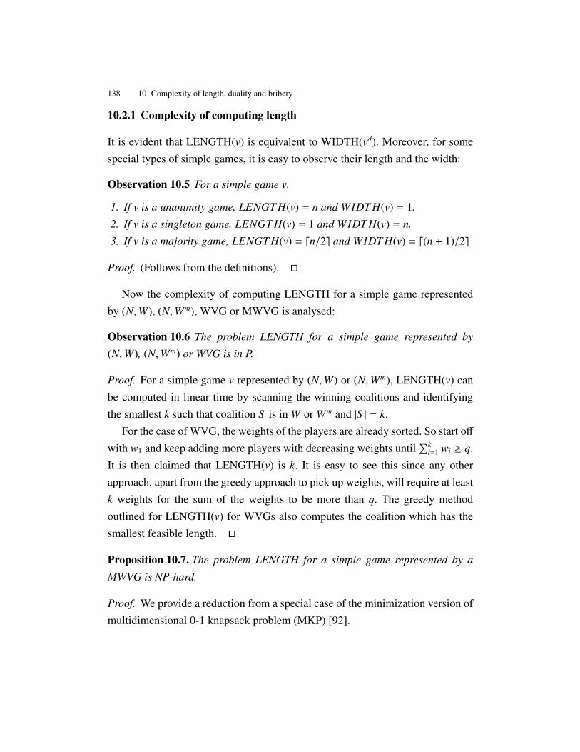
138 10 Complexity of length, duality and bribery
10.2.1 Complexity of computing length
It is evident that LENGTH(v) is equivalent to WIDTH(vd). Moreover, for somespecial types of simple games, it is easy to observe their length and the width:
Observation 10.5 For a simple game v,
1. If v is a unanimity game, LENGT H(v) = n and WIDT H(v) = 1.
2. If v is a singleton game, LENGT H(v) = 1 and WIDT H(v) = n.
3. If v is a majority game, LENGT H(v) = dn/2e and WIDT H(v) = d(n + 1)/2e
Proof. (Follows from the definitions). ut
Now the complexity of computing LENGTH for a simple game representedby (N,W), (N,Wm), WVG or MWVG is analysed:
Observation 10.6 The problem LENGTH for a simple game represented by
(N,W), (N,Wm) or WVG is in P.
Proof. For a simple game v represented by (N,W) or (N,Wm), LENGTH(v) canbe computed in linear time by scanning the winning coalitions and identifyingthe smallest k such that coalition S is in W or Wm and |S | = k.
For the case of WVG, the weights of the players are already sorted. So start off
with w1 and keep adding more players with decreasing weights until∑k
i=1 wi ≥ q.It is then claimed that LENGTH(v) is k. It is easy to see this since any otherapproach, apart from the greedy approach to pick up weights, will require at leastk weights for the sum of the weights to be more than q. The greedy methodoutlined for LENGTH(v) for WVGs also computes the coalition which has thesmallest feasible length. ut
Proposition 10.7. The problem LENGTH for a simple game represented by a
MWVG is NP-hard.
Proof. We provide a reduction from a special case of the minimization version ofmultidimensional 0-1 knapsack problem (MKP) [92].

10.2 Computing length of games 139
Name: MKPInstance: A collection of n items and m knapsacks where the capacity of the ithknapsack is bi, the jth item requires ai j units of resource consumption in the ithknapsack and has corresponding profit c j
Output: Maximize∑n
j=1 c jx j such that∑n
j=1 ai jx j ≤ bi, i ∈ M = {1, 2, . . .m}, andx j ∈ {0, 1}, j ∈ N = {1, 2, . . . n}.
The goal in MKP is to find a subset of items that yields maximum profit with-out exceeding the resource capacities. MKP is equivalent to the minimizationversion of the problem (MIN-MKP) since maximizing the profit of a set of itemsis equivalent to minimizing the profit of items not in the set. The transformationsneeded are y j = 1 − x j for j ∈ N and di = (
∑nj=1 ai j) − bi for j ∈ N and i ∈ M.
Therefore the following problem is as hard as MKP:
Name: MIN-MKPInstance: A collection of n items and m knapsacks where each knapsack i shouldhave at least di capacity filled and the jth item has corresponding profit c j andrequires ai j units of resource consumption.Output: Minimize
∑nj=1 c jy j such that
∑nj=1 ai jy j ≥ di, i ∈ M = {1, 2, . . .m} and
y j ∈ {0, 1}, j ∈ N.
Gens and Levner [96] point out that Dinic and Karzanov [61] proved that eventhe special case of MIN-MKP where m = 2 and c j = 1 for all j = 1 to n isNP-hard. It is easy to see that by renaming some variables (ai j to wi
j and di to qi),the NP-hard special case of MIN-MKP is equivalent to computing the length ofa MWVG of dimension 2. ut
10.2.2 Approximating the length of a MWVG
Although this may seem a paradox, all exact science is dominated by the
idea of approximation.
- Bertrand Russell

140 10 Complexity of length, duality and bribery
Although all NP-complete problems share the same worstcase complexity,
they have little else in common. When seen from almost any other per-
spective, they resume their healthy, confusing diversity. Approximability is
a case in point.
- Christos Papadimitriou (1993)
Although the length of a MWVG cannot be computed efficiently, it is observedthat it can be approximated efficiently:
Proposition 10.8. For a MWVG, v with dimension m, there exists a polynomial
time approximation algorithm which computes LENGTH(v) with an absolute er-
ror of m − 1.
Proof. This result uses the same approach as in [34] where the authors use LP-relaxation to provide an m − 1 absolute approximation algorithm for the Safe
Deposit Boxes (SDB) problem:
Name: Safe Deposit Boxes (SDB) problemInstance: a ji ≥ 0 for i = 1, . . . n and j = 1, . . .m.Output: Minimize
∑ni=1 xi such that
∑a jixi ≥ A j, j = 1, . . .m; x ∈ {0, 1},
i = 1, . . . , n.
A complete proof is given as follows. Let v be a MWVG with n players andm constituent WVGs [qt; wt
1, . . . ,wtn] for 1 ≤ t ≤ m. We assume that m < n.
The problem of computing LENGTH(v) is an integer program. An LP-relaxationchanges it into a problem where we want to minimize
∑ni=1 xi where
∑ni=1 xiwt
i ≥ qt
for all 1 ≤ t ≤ m and 0 ≤ xi ≤ 1 for all i ∈ N. The inequalities of the linearprogram can be changed into equalities by introducing n+m slack variable whereone slack variable is used for each inequality.

10.2 Computing length of games 141
min∑n
i=1 xi
s.t.∑n
i=1 xiwti + si = qt for i=1,. . . , m,
xi + sn+i = 1 for i=1,. . . , n,xi ≥ 0 for i=1,. . . , nsi ≥ 0 for i=1,. . . , m+n
(10.1)
The resultant LP has a total of n + m constraints and 2n + m variables (allof which are non-negative) where n + m is the number of slack variables. Anyextreme point in the feasible region of formulation requires n binding constraints.It follows that any basic feasible solution contains at least n zero values. Out ofthese n zero values, a maximum of m values can be attributed to slack variablesrelated to the quota constraints. Out of the remaining n−m zero values, either oneof the original variables is zero, or a slack variable related to the inequality xi ≤ 1is zero. In either of the cases, the original variable is non-fractional. Therefore,there are at most m original variables(xis) which may have fractional values inthe LP solution. The LP solution is of course solvable in polynomial time [44].
If none of the xis are fractional, then the LP solution is also the length of theMWVG. If not, then let l be the number of xis equal to one in the LP solution.Then, the length of the MWVG is at least l + 1. If we round up every fractionalvalues of the LP solution, then all the constraints are still satisfied. Moreover, themaximum value of the sum of the ceilings of values of the LP solution is l + m.Therefore the maximum error between the length of the MWVG and the sum ofthe ceilings of values of the LP solution is m − 1. ut
Although computing the length of an MWVG has a PTAS, there is no FP-TAS (fully polynomial time approximation scheme) [96]. The argument is thatif there is an ε-approximation algorithm polynomial in n and 1/ε to approximatethe length of a MWVG, then this implies that there is a polynomial algorithm tocompute the length of a MWVG.

142 10 Complexity of length, duality and bribery
10.3 Complexity of duality questions
Now some key problems on duality of simple games are defined.
Name: X-DUALIZATIONInstance: Simple game v in representation X.Output: Dual game vd in representation X
Name: DUALInstance: Simple games v and v′
Question: Are v and v′ dual of each other?
Name: SELF-DUALInstance: Simple games v
Question: Is v equivalent to vd?
It is noticed that in the dualization of a simple game v = (N,W), the output(N,W(vd)) may be exponential in terms of the input. For example take the una-nimity simple game v in which only the grand coalition is winning. Since everycoalition apart from the empty set is a blocking coalition, the dual of v has 2n − 1winning coalition. However, it is easy to decide DUAL for two simple gamesrepresented by their winning coalitions:
Proposition 10.9. DUAL for two simple games v = (N,W) and v′ = (N,W ′) is in
P.
Proof. If vd = v′, then |W | = 2n − |W ′|. This is because for each losing coalitionin v, its complement is winning in v′. In case |W | = 2n − |W ′|, then we considerthe bigger of the two sets |W | and |W ′|. Without loss of generality, let us assumethat |W | ≥ |W ′|. Then for each coalition S < W, we check if N \ S is a member ofW ′ or not. If N \ S is not a member of W ′, then return ‘no’. The total number ofsuch operations involved is (2n − |W |)(|W ′|) = (|W ′|
2). ut

10.3 Complexity of duality questions 143
It follows from the proposition that deciding the problem SELF-DUAL for asimple game (N,W) is in P.
Proposition 10.10. WVG-DUALIZATION is in P.
Proof. We denote by 〈q; w1, . . . ,wn〉 a WVG where a coalition S ⊂ N is winningif and only if w(S ) > q. For a WVG v = [q; w1, . . . ,wn] it is easy to see thatvd = 〈w(N) − q; w1, . . . ,wn〉. This observation has been made as early as in [63].The argument is that vd(S ) = 1 if and only if v(N \ S ) = 0. Take any coalitionS such that vd(S ) = 1. This means that w(S ) > w(N) − q which is equivalent tow(N \ S ) = w(N) − w(S ) < q. If WVG v is represented by integers only, thenvd = [w(N) − q + 1; w1, . . . ,wn]. ut
Corollary 10.11. For a WVG v, WIDTH(v) is in P.
Proof. For any simple game v, WIDTH(v) is equivalent to LENGTH(vd). Itis already known that WVG-DUALIZATION is in P and that for a WVG v,LENGTH(v) is in P. Therefore, computing the width of a WVG is in P. ut
Now, we examine the problem MWVG-DUALIZATION. Let v be a MWVGwhere its constituent WVGs are vt = [qt; wt
1, . . . ,wtn] for 1 ≤ t ≤ m. Also,
vd =∨m
t=1 vtd. We know that vt
d = [(∑n
i wti) − qt + 1; wt
1, . . . ,wtn]. Therefore while
dualizing a MWVG, it easy to get a disjunction of WVGs but not easy to geta MWVG. A dual of MWVG is also a simple game and therefore can be rep-resented by a MWVG. However, it will be interesting to check if the dual of aMWVG with dimension m can be represented by a MWVG with a dimensionpolynomial in m.
It is interesting to see that although computing the length of a MWVG is dif-ficult, the computing the width of a MWVG is computationally easy.
Proposition 10.12. For a MWVG v, WIDTH(v) is in P.
Proof. Let v be a MWVG where its constituent WVGs are vt = [qt; wt1, . . . ,w
tn] for
1 ≤ t ≤ m. Then, vd =∨m
t=1 vtd. We know that vt
d = [(∑n
i wti)− qt + 1; wt
1, . . . ,wtn].
Now we know that WIDTH(v) is equal to LENGTH(vd).

144 10 Complexity of length, duality and bribery
It is proved that LENGTH(vd) = Infnt=1{LENGTH(vt
d)}. Choose i ∈ {1, . . .m},such that length of vi
d is the smallest among vtds for all t. Then assume for con-
tradiction that there exists some coalition C ⊆ N such that C is winning in vd and|C| is less than the length of vi
d. Then then there exists a j ∈ {1, . . .m} other than i
such that v jd(C) = 1. This implies that the length of v j
d is less than the length ofvi
d which is a contradiction. ut
There is no known polynomial time algorithm for Wm-DUALIZATION. Nei-ther are there any hardness results for the problem. However it is known thatWm-DUALIZATION is polynomially time equivalent to the problems DUAL andSELF-DUAL for simple games represented by their MWCs [37, 86]. It is alsoknown that linear simple games represented by MWCs can be dualized in poly-nomial time [66]. Now we prove that the complexity of DUAL for WVGs isNP-hard:
Proposition 10.13. DUAL for WVGs is co-NP-complete.
Proof. We first define another problem EQUIVALENT-WVGs:
Name: EQUIVALENT-WVGsInstance: WVGs v = [q; w1, . . . ,wn] and v′ = [q′; w1
′, . . . ,wn′]
Question: Is v = v′?
We first prove that this problem is NP-hard. We provide a reduction fromthe problem of checking whether a player is a dummy or not. Let v by a WVG[10q+1; 10w1, . . . , 10wn−1, 1] where q and wis are all integers. It is known that it isNP-hard to verify whether player n with weight 1 is a dummy or not [151]. This isequivalent to asking whether v is equivalent to WVG [10q; 10w1, . . . , 10wn−1, 0].Moreover, it is easy to see that EQUIVALENT-WVGs is in co-NP because anycoalition S such that v(S ) , v′(S ) is a ‘no’ certificate.
Now that we know that EQUIVALENT-WVGs is NP-hard we show thatany instance of EQUIVALENT-WVGs is equivalent to the problem DUAL forWVGs. We take an instance of EQUIVALENT-WVGs where we want to check

10.4 Bribery in WVGs 145
whether WVGs v = [q; w1, . . . ,wn] and v′ = [q′; w1′, . . . ,wn
′] are equivalent. Thisis the same as asking whether the dual of v′ is [w(N) − q + 1; w1, . . . ,wn]. ut
From the proof it follows that SELF-DUAL for WVGs is also co-NP-complete.Moreover, DUAL and SELF-DUAL for MWVGs are co-NP-complete. For a pairof simple games represented by their winning coalitions, both games have to beexactly similar for them to be equivalent. The same rule holds for simple gamesrepresented by their minimal winning coalitions.
10.4 Bribery in WVGs
Manipulation, control and bribery in elections and social choice protocols havebeen examined both in political science and multiagent systems. In [75], a com-prehensive analysis of manipulation in elections was undertaken. Different kindsof manipulations considered are insincere behaviour by voters, bribery of votersand control by mechanism designers. Manipulations in voting systems have re-ceived interest in many recent papers, for instance [104, 180, 50]. In this section,a similar approach is used to analyse bribery in simple games.
Winning coalitions with the smallest length are the following set: We = {S :S ⊂ W, |S | ≤ |S ′| ∀S ′ ∈ W}. For the specific case of WVGs, another variationis winning coalitions with the minimum weight: W s = {S : S ⊂ W,w(S ) ≤w(S ′) ∀S ′ ∈ W}. It is evident that We and W s are subsets of Wm. These kindsof minimal winning coalitions have also been considered in [51]. Both W s andWe appear to be useful concepts especially from the point of view of briberyand manipulation in social choice protocols. If a manipulator wants to control ormanipulate a coalition, he would prefer a coalition which is winning but barely,with minimal weight or number of players. Minimizing the number of playersbribed has the motivation of maximizing confidentiality and minimizing costs.Minimizing the weight of the bribed coalition has motivation in the assumptionthat players may price themselves according to their perceived importance, whichis their contributed weight. For example, if each player has unit cost of being in-fluenced, the cost of bribery is the length of the game. The general problem is

146 10 Complexity of length, duality and bribery
defined as follows:
Name: SVG-WIN-BRIBERYInstance: Simple game v with cost ci for each player i ∈ N.Output: Minimize the bribery cost while ensuring a win.
10.4.1 Under no information
We now examine the complexity of optimal bribery to ensure the decision whenthere is no information on the players’ preferences (whether they want to vote‘yes’ or ‘no’).
Influencing a decision
Proposition 10.14. SVG-WIN-BRIBERY is in P for a simple game represented by
a WVG, (N,W) or (N,Wm) where each player has unit cost and the manipulator
has no knowledge of player preferences.
Proof. This follows directly from Observation 10.6) that computing a winningcoalition with the minimum number of players can be computed in polynomialtime for all the three representations. ut
Proposition 10.15. SVG-WIN-BRIBERY is NP-hard for a MWVG where each
player has unit cost and the manipulator has no knowledge of player preferences.
Proof. This follows from the result that computing LENGTH(v) of MWVGs isNP-hard. ut
Since we noticed that LENGTH(v) for MWVG has an absolute error approx-imation algorithm, this means that SVG-WIN-BRIBERY also be approximatedefficiently. As the approximation algorithm always overestimates the length of theMWVG, it is guaranteed that a big enough coalition of players has been bribed.

10.4 Bribery in WVGs 147
Proposition 10.16. SVG-WIN-BRIBERY is NP-hard for WVGs where each player
has cost proportional to its weight and the manipulator has no knowledge of
player preferences.
Proof. We use a reduction from the optimization version of the SUBSET-SUMProblem where the instance is A = {a1, . . . , ak} and we want to minimize
∑ki=1 xiai
such that∑k
i=1 xiai ≥ Q where xi ∈ {0, 1}. This problem is equivalent to SVG-WIN-BRIBERY which involves minimizing
∑ki=1 xi(Cwi) such that
∑ki=1 xiwi ≥ Q
where xi ∈ {0, 1}, wi = ai for all i = 1 to k and C is a constant. ut
Maintaining the status quo
If a manipulator wants to maintain the status quo and prevent the formation ofa winning coalition, he might want to control a blocking coalition with the leastcost. This could again be a coalition which is winning in the dual of the game buteither has the smallest number of players or the least amount of weight.
Name: SVG-VETO-BRIBERYInstance: Simple game v with cost ci for each player i ∈ N.Output: Ensure a no-win (so that a decision cannot be taken) while minimizingcost.
It is easy to see that SVG-VETO-BRIBERY for WVG v is equivalent toSVG-WIN-BRIBERY for vd. Therefore, we automatically arrive at the follow-ing propositions:
Proposition 10.17. If the manipulator has no knowledge of player preferences,
1. SVG-VETO-BRIBERY is in P for a WVG where each player has unit cost.
2. SVG-VETO-BRIBERY is in P for a MWVG where each player has unit cost.
3. SVG-VETO-BRIBERY is NP-hard for a WVG where each player has cost pro-
portional to its weight.
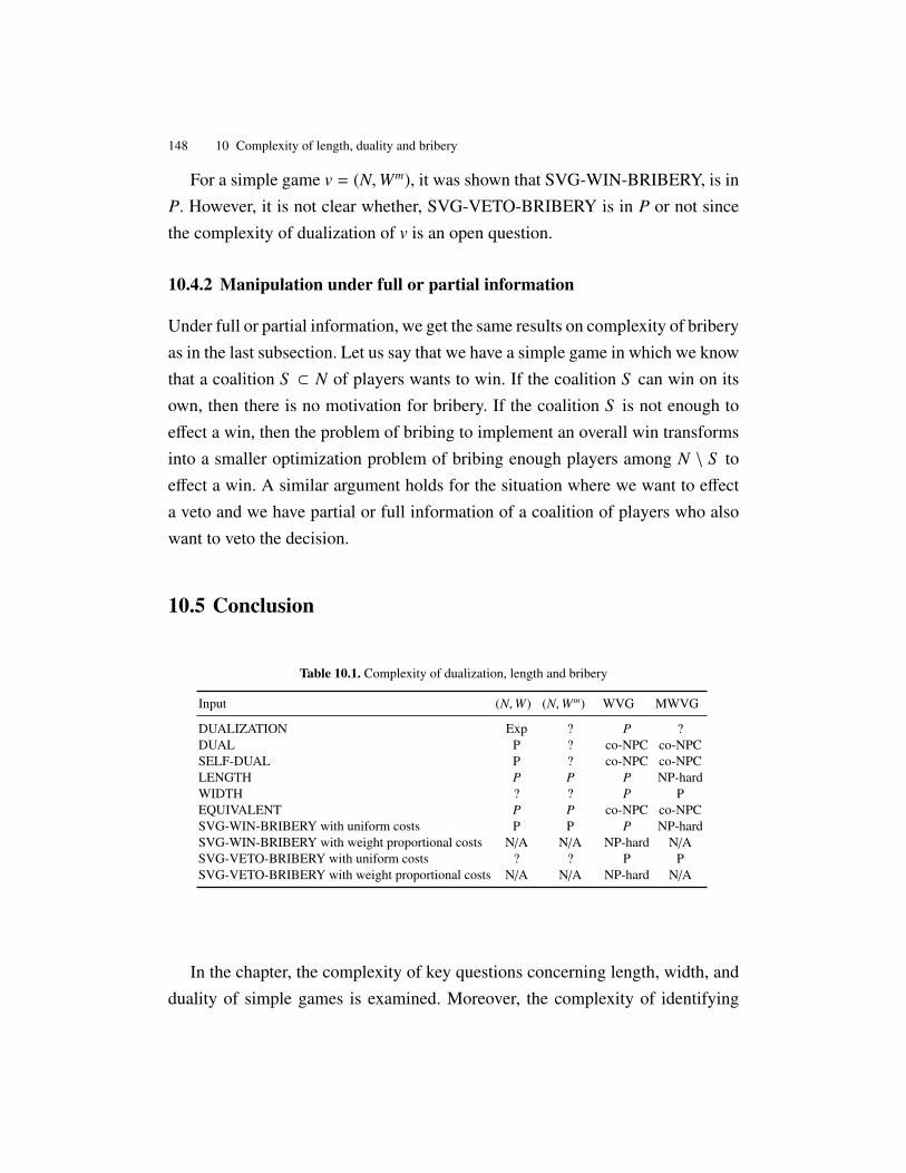
148 10 Complexity of length, duality and bribery
For a simple game v = (N,Wm), it was shown that SVG-WIN-BRIBERY, is inP. However, it is not clear whether, SVG-VETO-BRIBERY is in P or not sincethe complexity of dualization of v is an open question.
10.4.2 Manipulation under full or partial information
Under full or partial information, we get the same results on complexity of briberyas in the last subsection. Let us say that we have a simple game in which we knowthat a coalition S ⊂ N of players wants to win. If the coalition S can win on itsown, then there is no motivation for bribery. If the coalition S is not enough toeffect a win, then the problem of bribing to implement an overall win transformsinto a smaller optimization problem of bribing enough players among N \ S toeffect a win. A similar argument holds for the situation where we want to effecta veto and we have partial or full information of a coalition of players who alsowant to veto the decision.
10.5 Conclusion
Table 10.1. Complexity of dualization, length and bribery
Input (N,W) (N,Wm) WVG MWVG
DUALIZATION Exp ? P ?DUAL P ? co-NPC co-NPCSELF-DUAL P ? co-NPC co-NPCLENGTH P P P NP-hardWIDTH ? ? P PEQUIVALENT P P co-NPC co-NPCSVG-WIN-BRIBERY with uniform costs P P P NP-hardSVG-WIN-BRIBERY with weight proportional costs N/A N/A NP-hard N/ASVG-VETO-BRIBERY with uniform costs ? ? P PSVG-VETO-BRIBERY with weight proportional costs N/A N/A NP-hard N/A
In the chapter, the complexity of key questions concerning length, width, andduality of simple games is examined. Moreover, the complexity of identifying

10.5 Conclusion 149
the ideal coalition to bribe has been considered for different cost patterns. A sum-mary of results is presented in Table 10.1. The question marks indicate problemswhich are open. It is seen that since simple games involve binary decisions, thebribery process is not as complex as general elections with a range of alternatives.However, optimal bribery has different complexity for different representations ofgames and approaches to bribery. The idea of optimal bribery may be a realisticconsideration if there are multiple decisions to be made via simple games, andthe briber does not want to overuse his resources. In analyzing bribery, it willbe more realistic to consider probabilistic models where there are probabilitiesfor players to vote ‘yes’ or ‘no’. In this context, results from information the-ory might shed more light. Another direction is to examine simple games whereinstead of deciding a binary outcome, the players vote for a list of candidates.Moreover, characterizing the complexity of dualization of simple games repre-sented by MWCs is a long-standing open question.


Part IV
Resource Allocation & Networks


11
Cooperative game theory & simple games
The value or worth of a man is, as of all other things, his price; that is to
say, so much as would be given for the use of his power, and therefore is
not absolute, but a thing dependent on the need and judgement of another.
- Thomas Hobbes (Leviathan)
In seeking private interests, we fail to secure greater collective interests.
The narrow rationality of self-interest that can benefit us all in market
exchange can also prevent us from succeeding in collective endeavors.
- Russell Hardin (Collective Actions)
The classes of problems which are respectively known and not known to
have good algorithms are of great theoretical interest ... I conjecture that
there is no good algorithm for the traveling salesman problem. My reasons
are the same as for any mathematical conjecture: (1) it is a legitimate
mathematical possibility; and (2) I do not know.
- Edmonds (1966)
Abstract Simple coalitional games are not only a type of voting games but alsoa fundamental class of cooperative games. In this chapter, cooperative games andcooperative game solutions are introduced. Cooperative game theory is concernedwith analyzing which coalitions will form and how should the coalitions dividethe payoff between their members. The trend of using computational tractability
154 11 Cooperative game theory & simple games
as a criterion for cooperative game solutions is recent and is prevalent in the math-ematics of operations research and theoretical computer science. In this chapter,the computational aspects of various cooperative game solutions in simple gamesare examined. Questions considered include the following: 1) for solution set X
and simple game v, is X of v empty or not, 2) compute an element in X of v
and 3) verify if a payoff is in X of v. Some representations taken into accountare simple games represented by W, Wm, WVGs and MWVGs. The cooperativesolutions considered are the core, ε-core, least-core, nucleolus, prekernel, kernel,bargaining set and stable sets. A complexity of checking the stability of the coreof simple games is also examined. Structural results of the least core and nu-cleolus payoffs of simple games are presented. A theorem from the paper “Thenucleolus and kernel for simple games or special valid inequalities for 0 − 1 lin-ear integer programs” by L.A Wolsey is corrected. It is proved that an oracle tocompute a least core payoff for a simple game in any passer-reasonable repre-sentation can be used to compute the worst excess of a least core payoff. Finally,the relation between cost of stability and the least core is examined. A natural anddesirable solution called the super-nucleolus is also proposed.
11.1 Introduction and background
Cooperative game theory models problems where a group of players cooperate tomake a profit or investment and the profit or cost has to be allocated among theplayers in a fair and stable way. If a subset of players in N cooperate and worktogether, they form a coalition. Cooperative game theory is used to analyse whichcoalitions will form and how the coalitions should divide the payoff among theirmembers. Solution concepts in cooperative theory measure profit allocations ofplayers while considering the profit of each coalition of players. The foundationsof cooperative game theory were laid by von Neumann and Morgenstern. Thebiggest focus in the development of cooperative game theory has been devisingvarious solution concepts to explain equilibrium in different systems. This alsoinvolved axiomatic characterization of the properties of the solution concepts andtheir relations with each other.

11.3 Preliminaries 155
11.2 Related work
Cooperative game theory has seen tremendous growth in the last few decadeswith several textbooks written on it [196, 163, 62, 176]. Concepts from the areahave then been used in various combinatorial optimization games in operationsresearch which involve resource allocation among multiple players [54, 38]. Al-though algorithms to compute different solutions have been considered in themathematics of operations research literature, Deng and Papadimitriou [60] un-dertook one of the earliest computational complexity investigation of differentsolution concepts. There have been new developments in the computational com-plexity of solution concepts of weighted voting games [68, 70]. Deng and Fanghave surveyed the developments in algorithmic cooperative game theory in a re-cent detailed article [58]. Cooperative game theory has also been widely usedby the artificial intelligence and multiagent community, especially for multiagentresource allocation [46].
11.3 Preliminaries
We define different kinds of cooperative games. The definitions are to providecontext and to show how simple games are related to other classes of games.The relations between the classes of cooperative games are further highlighted inFigure 11.1 and Figure 11.2.
Definitions 11.1. A cooperative game is:
• zero-normalized if v({i}) = 0 for all i ∈ N,
• monotonic if S ⊆ T ⊆ N implies that v(S ) ≤ v(T ),• superadditive if for all S ,T ⊂ N, if S ∩ T = ∅, then v(S ∪ T ) ≥ v(S ) + v(T ),• cohesive if v(N) ≥
∑Kk=1 v(S k) for every partition {S 1, . . . , S k} of N,
• additive if for all S ,T ⊂ N, if S ∩ T = ∅, then v(S ∪ T ) = v(S ) + v(T ),• constant-sum if for all S ⊂ N, v(S ) + v(N \ S ) = v(N),• convex if v(S ∪ T ) ≥ v(S ) + v(T ) − v(S ∩ T ) for all S ,T ⊂ N.
156 11 Cooperative game theory & simple games
Among cooperative games, simple coalitional games are a fundamental sub-class of games because any cooperative game can be mapped into a correspondingsimple game by introducing a threshold which is a value between zero and thevalue of the grand coalition. In the simple game variation, a coalition which hasa value greater than or equal to the threshold may be considered winning. Well-studied games such as threshold network flow games [26] fit into this framework.
Definition 11.2. For each cooperative game (N, v) and each threshold t ∈ R+, the
corresponding threshold game or version is defined as the cooperative game (N, vt),where
vt(S ) =
1 if v(S ) ≥ k,
0 otherwise.
It is easily verified that, for any threshold t, if a game (N, v) is monotone, so is itsthreshold version (N, vt), in which case (N, vt) is a simple game.
A weighted voting game is homogeneous if it can have a homogeneous repre-
sentation. A WVG is a homogeneous representation if all minimal winning coali-tions have the same weight. This implies that in a homogeneous representation,players with equal power get the same weight.
Observation 11.3 We recall that a decisive simple game is one which is both
proper and strong (Definition 2.5). Therefore, it easy to see that a constant-sum
game which is simple is equivalent to a decisive simple game.
A solution concept assigns for each game a set of payoffs or allocations. TheBanzhaf index can also be considered as a solution concept specifically in thecontext of simple games. We will generally denote a payoff by a vector x =
(x1, . . . , xn) where xi is the payoff of player i for i ∈ N. The choice of a specificsolution concept depends on the notion of fairness, stability and certain desirableproperties. We write x(S ) for
∑i∈S xi
Definitions 11.4. Some desirable properties of payoffs for solution concepts are:
• Efficiency: For any game (N, v),∑
i∈N xi = v(N).

11.3 Preliminaries 157
Cohesive Supper-additive
Convex
Additive
Fig. 11.1. Relations of cooperative games I
WVG
Simple
Additive
Proper simple
Constant-sum Linear Simple
Fig. 11.2. Relations of cooperative games II
• Individual rationality: xi ≥ v(i) for all i ∈ N. This means the payoff of a player
is at least the amount which it can get by acting alone in the game.
• Coalitional rationality: x(S ) ≥ v(S ) for all S ⊆ N.
• Nonemptiness: The set of payoffs according to the solution concept is non-
empty for any game (N, v).• Computationally feasible: The solution concept can be computed efficiently.
• Symmetry: The solution concept is not influenced by renumbering of the
player set. The condition is also referred to as anonymity in the literature.
158 11 Cooperative game theory & simple games
• Additive: For any two v1 and v2, xi(v1 + v2) = xi(v1) + xi(v2) where game
(N, v1 + v2) is such that (v1 + v2)(S ) = v1(S ) + v2(S ) for any coalition S .
• Zero allocation to Dummies: If i is a dummy player, then xi(v) = v({i}) = 0.
• Pareto optimal: If x, y are two payoffs such that xi > yi for all i ∈ N, then y is
not in the solution.
We define different types of payoffs depending on which desirable properties theysatisfy:
Definitions 11.5. Different kind of payoffs in cooperative games are:
• Feasible payoff: For a cooperative game (N, v), a feasible payoff is x ∈ Rn
such that x(N) ≤ v(N). The set of feasible payoffs is denoted by X∗(N, v).• Preimputation: For a cooperative game (N, v), a preimputation is x ∈ Rn such
that x(N) = v(N). Preimputations are efficient feasible payoffs. The set of
preimputations for a game v is denoted by I∗(v).• Imputation: For a cooperative game (N, v), an imputation x is a preimputation
which satisfies individual rationality, i.e. such that for all i ∈ N, x(i) ≥ v(i).The set of imputations for a game v is denoted by I(v).
11.4 Cooperative game theory solutions
11.4.1 Introduction
In cooperative game theory, the goal is to distribute the payoffs fairly amongthe players and encourage cooperation. Solution concepts formalize the notionsof fair and stable payoffs. For a payoff x = (x1, ..., xn), the excess e(x, S ) of acoalition S under x is x(S ) − v(S ). The excess vector of a payoff x, is the vec-tor (e(x, S 1), ..., e(x, S 2n)) where e(x, S 1) ≤ e(x, S 2) ≤ e(x, S 2n). We denote thedistinct values in the excess vector by −ε1(x, v),−ε2(x, v), . . . ,−εm(x, v) where−εi(x, v) < −ε j(x, v) for i < j. For a payoff x and game v, the set of coalitions thatget the i-th distinct worst excess −εi(x, v) will be denoted by Ai
x(v) and a memberof Ai
x(v) will be called an εi-coalition. Many of the following definitions are from[68] and [163]. A payoff x is called an S -feasible payoff vector if x(S ) = v(S ).

11.4 Cooperative game theory solutions 159
An N-feasible payoff vector which is a preimputation is called a feasible payoff
profile.We consider the following cooperative game solutions for simple game: Shap-
ley value, core, ε-core, nucleolus [149], stable set [141], bargaining set [149],kernel [149], prekernel and τ-value. The core of a game is one of the most fun-damental solutions in cooperative game theory. The idea of the core goes backto von Neumann and Morgenstern [213]. The modern definition and name werefirst used in [98].
Definition 11.6. Core: A payoff x is in the core if and only ∀S ⊂ N, e(x, S ) ≥ 0or in other words x(S ) ≥ v(S ). The core of a game (N, v) is denoted by C(v) and
C(v) ⊂ I(v).
A core imputation guarantees that each coalition gets at least what it couldgain on its own. The core is not unique and is a set which satisfies a system ofweak linear inequalities, so it is closed and convex. Moreover, the core is well-defined, but can be empty. Those games which have non-empty cores are calledbalanced. Although the core is a desirable solution concept, it may be empty formany games. This led to the development of ε-core [193] and least core [142].
Definitions 11.7. A preimputation x is in the ε-core if ∀S ⊂ N, e(x, S ) ≥ −ε. The
ε-core is denoted by Cε(v). The preimputation x is in the least core if it is in the
ε-core for the smallest possible ε. We will denote by −ε1(v), the worst excess of
any least core payoff of (N, v).
Therefore, the least core is the intersection of all the ε-cores. The least core isnot unique and may contain many payoffs. One may want to find fairest payoffsamong the payoffs within the least core. This led to the idea of the prenucleolus
and nucleolus [189].
Definition 11.8. Prenucleolus: A preimputation x that has lexicographically the
largest excess vector is called the prenucleolus.
Definition 11.9. Nucleolus: An imputation x that has lexicographically the largest
excess vector is called the nucleolus.

160 11 Cooperative game theory & simple games
The prenucleolus always exists and is unique as long as v(S ) = 0 for all oneperson coalitions [189]. It is easy to see that the least core is always non-emptyand always contains the prenucleolus. For any cooperative game v for which I(v)is non-empty, the nucleolus also exists and coincides with the prenucleolus. Interms of the computational complexity of problems concerning nucleolus andprenucleolus, there is no difference.
Definition 11.10. Stable Set: An imputation x dominates imputation y if there is
a non-empty coalition S such that xi > yi for all i ∈ S and x(S ) ≤ v(S ). Two
imputations can dominate each other. A stable set of a game (also known as the
von Neumann-Morgenstern solution [213]) is a set of imputations which satisfies
the following two properties:
1. Internal stability: No imputation in the stable set is dominated by another
imputation in the set.
2. External stability: All imputation outside the set are dominated by at least one
alternative in the set.
A stable set may or may not exist [140]. Moreover, just like the core, even if itexists it is not necessarily a singleton. [139]. For zero-normalized simple games,stable sets always exist. It is also known that the core is a subset of any stable setand if the core is stable it is the unique stable set [62].
The bargaining set models stability of payoffs where if player i has an objec-tion against player j to imputation x, then j has a counter-objection.
Definition 11.11. Bargaining set: The pair (y, S ), where S is a coalition, is an
objection of i against j to x if S includes i but not j, y(S ) = v(S ) and yk > xk
for all k ∈ S . A pair (z,T ) where T is a coalition is a counter-objection to theobjection (y, S ) of i against j if T includes j, but not i, z(T ) = v(T ), zk ≥ xk for all
k ∈ T \S and zk ≥ yk for all k ∈ T⋂
S . An imputation x belongs to the bargainingset M(v) of game v, if for any objection (y, S ) of any player i against player j to
x, there is a counter-objection to (y, S ) by j to x.
The kernel is a subset of the bargaining set with similar concept of objectionsand counter-objections.
11.4 Cooperative game theory solutions 161
Definition 11.12. Kernel: A coalition, S is an kernel-objection of i against j tox if S includes i but not j and x j > v({ j}). A coalition, T is the kernel-counter-objection to the objection S of i against j if T includes j but not i and e(x,T ) ≤e(x, S ). The kernel of a coalitional game with transferable payoffs is the set of all
imputations x with the property that for every objection S of any player i against
any other player j to x there is a counter-objection of j to S . The kernel of a
simple game (N, v) is denoted by K(v). There is also an alternative way to define
the kernel. We let svi j(x) be the maximum surplus of player i over player j with
respect to x, i.e.,
svi j(x) = max {v(S ) − x(S )|S ⊆ N \ { j}, i ∈ S } .
Then the kernel is the set of imputations x such that
(svi j(x) − sv
ji(x))(x j − v({ j})) ≤ 0
and
(svji(x) − sv
i j(x))(xi − v({i})) ≤ 0.
We say that i outweighs j according to payoff x if svi j(x) > sv
ji(x) and x j >
v({ j}). This is equivalent to saying that i has an objection against x to j for which
j has no counter-objection.
Definition 11.13. Prekernel: The prekernel of a game (N, v) is the set of preim-
putations x ∈ I∗(v) such that:
svi j(x) = sv
ji(x)
for all i, j. The prekernel of the game (N, v) is denoted by PK(v).
We see that simple games with no passers are both zero-normalized and alsozero-monotonic.
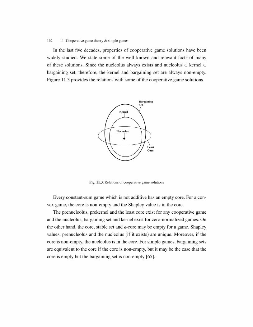
162 11 Cooperative game theory & simple games
In the last five decades, properties of cooperative game solutions have beenwidely studied. We state some of the well known and relevant facts of manyof these solutions. Since the nucleolus always exists and nucleolus ⊂ kernel ⊂bargaining set, therefore, the kernel and bargaining set are always non-empty.Figure 11.3 provides the relations with some of the cooperative game solutions.
Bargaining Set
Kernel
Least Core
Nucleolus
Fig. 11.3. Relations of cooperative game solutions
Every constant-sum game which is not additive has an empty core. For a con-vex game, the core is non-empty and the Shapley value is in the core.
The prenucleolus, prekernel and the least core exist for any cooperative gameand the nucleolus, bargaining set and kernel exist for zero-normalized games. Onthe other hand, the core, stable set and ε-core may be empty for a game. Shapleyvalues, prenucleolus and the nucleolus (if it exists) are unique. Moreover, if thecore is non-empty, the nucleolus is in the core. For simple games, bargaining setsare equivalent to the core if the core is non-empty, but it may be the case that thecore is empty but the bargaining set is non-empty [65].

11.4 Cooperative game theory solutions 163
11.4.2 Desirability relation and cooperative game solutions
For simple games, we consider respecting the desirability relation in a simplegame as another useful criterion for a solution concept. A payoff x obeys desir-ability relations if when i is more desirable than j, then xi ≥ x j. Table 11.1 listscooperative game solutions and whether they respect the desirability relation.
Table 11.1. Cooperative game solutions and desirability relation in simple games
Cooperative game solution Desirability relationBanzhaf index XShapley-Shubik index XHoller index XDeegan-Packel Index 5
Nucleolus XPrekernel XKernel XBargaining Set 5
Core 5
Least core 5
11.4.3 Generalized problems
We define some natural problems in cooperative game theory. For the sake ofconsistency and continuity, we have used the same names for the problems as in[68] where single WVG are analysed.
Name: EMPTY-XInstance: Simple game v
Question: Is X empty?
Name: IN-XInstance: Simple game v and payoff p
Question: Is p in solution X of v?
164 11 Cooperative game theory & simple games
Name: CONSTRUCT-XInstance: Simple game v
Output: A payoff p which is in solution X of v?
Name: ISZERO-XInstance: Simple game v and player i
Question: Is payoff of player i in game v zero according to solution X?
For a solution X which is unique, the problem IN-X is equivalent to checkingif a payoff is X and the problem CONSTRUCT-X is equivalent to computing X.If a solution X is not unique, then the problem ISZERO-X is not precise and wewill ignore it. Moreover if X is unique, then we will consider CONSTRUCT-Xsimply as computing X.
11.5 Core
Proposition 11.14. For a simple game (N, v), I(v) is non-empty if and only if there
is at most one passer.
Proof. I(v) is non-empty if and only if there exists a payoff x such that x(N) = 1and xi ≥ v({i}) for all i ∈ N. This is true if and only if either v({i}) = 0 for alli ∈ N, or there exists a unique j ∈ N such that v({ j}) = 1. If j is the unique passer,then x is an imputation if and only if x j = 1. ut
If there is a passer, then no other player can be a vetoer. Elkind et al. [68]showed that EMPTY-CORE is in P for WVGs. We notice that this observationholds true for simple games in any representation:
Proposition 11.15. EMPTY-CORE is in P for simple games in any representation
where the value of a coalition is obtained in polynomial time.
Proof. We first observe that EMPTY-CORE for a simple game v is equivalent toverifying that IDENTIFY-VETOERS is an empty set. The argument for this is

11.6 Core stability 165
as follows. We want to prove that the core of a simple game is non-empty if andonly if a vetoer exists.
(⇒) Let us assume that the core is non-empty and there is a feasible imputationp which is in the core. Let us also assume that no vetoer exists. Take any playerj with non-zero imputation according to x. Since j is not a vetoer, v(N \ { j}) = 1.However p(N \ { j}) < 1 is a contradiction since x is in the core.
(⇐) We now prove that if a vetoer exists, the core is non-empty. We knowthat v(N) = 1 and p(N) = 1. If a vetoer i exists, our imputation p is such thatwe can give all the payoff to i, and none to the other players. In that case for allS ⊆ N \ {i}, p(S ) = 0 and v(S ) = 0. Therefore p is in the core and the core isnon-empty.
Identifying vetoers is easy for any representation of a simple game for whichvalue of each coalition can computer in polynomial time. A player i is a vetoerif and only if v(N \ {i}) = 0. A simple game even with an implicit characteristicfunction can return v(N \ {i}). Therefore IDENTIFY-VETOERS can be used in ablack-box manner to solve EMPTY-CORE. ut
Elkind et al. [68] prove that if the core of simple game v is non-empty, thenucleolus of v is given by xi = 1/k if i is vetoer and xi = 0 if i is not a vetoer,where k is the total number of vetoers. The result also holds even if we considerany element of the kernel and any simple game [9]. Therefore, for a simple gamev represented by (N,W), (N,Wm), WVG, MWVG or any other representation, ifthe core is non-empty, the nucleolus can be computed in polynomial time.
11.6 Core stability
It is already known that the core is a subset of every stable set, no stable set is asubset of another stable set and if the core is a stable set then it is the only stableset (Prop 279.2a [163]). The following is a characterization of the stable set of asimple game:
Proposition 11.16. For a simple game v, a set of imputations is a stable set if and
only if for some minimal winning coalition T , all players not in T get zero payoff.

166 11 Cooperative game theory & simple games
Proof. (⇐)If T be a minimal winning coalition. Then the claim is that XT = {x|x(T ) = 1}
is a stable set. The set is internally stable because there is no imputation y ∈
XT such that there exists a non-empty coalition S such that xi < yi for i ∈ S .Moreover, let z be an imputation not in XT . Then z(T ) < x(T ), which impliesthere exists an x ∈ XT which dominates z. Therefore, constructing a stable set ofa simple game simply requires identifying a minimal winning coalition.
(⇒) Let us assume that Y is a stable set of imputations of game v such thatthere exists at least one imputation y ∈ Y which does not distribute all its payoff
exactly to players in a minimal winning coalition. This means that that y dis-tributes its payoff to a coalition T ′′ such that T ′′ ⊃ T where T is a minimalwinning coalition. However, it is easy to see that y is dominated by an imputationin XT . ut
Corollary 11.17. CONSTRUCT-STABLE-SET and IN-STABLE-SET are in P for
any representation of a simple game where the value of a coalition is obtained in
polynomial time.
The stability of the core is an important question in algorithmic cooperativegame theory. Core stability has been examined for several classes of games in-cluding assignment games [183], minimum coloring games [35], network flowgames [200] and vertex cover games [79]. However for simple games, a stableset always exists. The following is a characterization of the core stability of sim-ple games.
Proposition 11.18. The core of a simple game is stable if and only if there is only
one minimal winning coalition of the game.
Proof. If coalition S is the only MWC of the simple game v, then all players inS are vetoers. Any imputation which distributes the payoff among players in S
in the core. Moreover, from Proposition 11.16, we see that that the core is also astable set.
There is an alternative way to see this. A cooperative game is convex if v(S ∪T ) ≥ v(S ) + v(T ) − v(S ∩ T ) for all S ,T ∈ 2N where S , T . Moreover, there is a

11.7 Least core 167
well known result due to Shapley [191] that for convex games, the core is stable.We see that a simple game is not convex if and only if there exist coalitions S
and T , S , T such that v(S ) = 1, v(T ) = 1 and v(S ∩ T ) = 0. Then it followsthat v(S ∪ T ) = 1. If S and T are mutually exclusive then this means that thereare two MWCs. If S and T are not mutually exclusive then this means that S ∩ T
does not contain a MWC but S and T both contain MWCs. ut
Corollary 11.19. CORE-STABILITY is in P for any representation of a simple
game where the value of a coalition is obtained in polynomial time.
Proof. The problem is to check whether the simple game has only one MWC ornot. This is trivial for (N,Wm). For other representations, one needs to identifythe vetoers and then verify if the coalition of vetoers forms a winning coalition.This can be checked in polynomial time. ut
11.7 Least core
Elkind et al.(Theorem 5, [68]) proved that the problems EMPTY-ε-CORE, IN-LEASTCORE and CONSTRUCT-LEASTCORE are NP-hard for WVGs. SinceEMPTY-ε-CORE is NP-hard, then it follows that CONSTRUCT-ε-CORE is NP-hard. Also, from the proof in Theorem 5, [68], it is easy to see that IN-ε-COREis NP-hard.
It is easy to see from the definition of the least core, that it is the solution ofthe following LP:
min εs.t. x(S ) ≥ v(S ) − ε , for all S ⊂ N ,
xi ≥ 0 , for all i ∈ N,∑i=1,...,n xi = v(N) .
(11.1)
We now show that the for any simple games and least core payoff, every playeris in one coalition which gets the worst excess. Proposition 11.20 is speciallyfor simple games but as we shall see later, it can be generalized to monotonecooperative games.

168 11 Cooperative game theory & simple games
Proposition 11.20. For any simple coalitional game (N, v), suppose that x =
(x1, . . . , xn) is an element in the least core, where the minimum excess is −ε. Then
for any player i ∈ N there exists a coalition T such that i ∈ T and e(x,T ) = −ε.
Proof. Let A be the set of players such that for every j ∈ A, we have that j iscontained in some coalition M with e(x,M) = −ε. Consider a player i ∈ N \ A.We must have xi > 0, since if xi = 0, then for any coalition S such that i < S
and e(x, S ) = −ε, the excess e(x, S ∪ {i}) = −ε. Let δ be half of the minimumof the non-zero differences between successive components of the excess vectorof x. Then we can obtain a new imputation y such that yi = xi − Min(xi, δ), andy j = x j +
Min(xi,δ)|A| for j ∈ A, and yk = xk for k < A ∪ {i}. Since the smallest
excess for y is more than −ε, this means that x is not in the least core which is acontradiction. ut
Corollary 11.21. Suppose x = (x1, . . . , xn) is the nucleolus of a simple game. Let
e(x, S ) be the first element of the excess vector of x. Then for any player i , there
exists a coalition T such that i ∈ T and e(x,T ) = e(x, S ).
Proof. This follows from the fact that the nucleolus is a member of the least core.ut
We see that Proposition 11.20 can be generalized to monotone cooperativegames:
Proposition 11.22. For any monotone cooperative game (N, v), suppose that x =
(x1, . . . , xn) is an element in the least core, where the minimum excess is −ε. Then
for any player i ∈ N there exists a coalition T such that i ∈ T and e(x,T ) = −ε.
Proof. Let A be the set of players such that for every j ∈ A, we have that j iscontained in some coalition M with e(x,M) = −ε. Let P1 be the set of thosecoalitions which get an excess of −ε. Consider a player i ∈ N \ A.
Consider the case xi = 0. Choose a coalition S ∈ P1. Then we consider thecoalition S ∪ {i}. If v(S ∪ {i}) = v(S ), then i ∈ A. If v(S ∪ {i}) > v(S ), thene(x, S ∪ {i}) < −ε which is a contradiction.

11.7 Least core 169
Now consider the case when xi > 0. Let δ be half of the minimum of thenon-zero differences between successive components of the excess vector of x. Ifthere exists a coalition S ∈ P1 such that x(S ∪ {i})− v(S ∪ {i}) < −ε, then this is acontradiction. If there exists a coalition S ∈ P1 such that x(S∪{i})−v(S∪{i}) = −ε,then i ∈ A. If there exists no coalition S ∈ P1 such that x(S ∪{i})−v(S ∪{i}) ≤ −ε,then we can obtain a new payoff y such that yi = xi − Min(xi, δ), and y j = x j +Min(xi,δ)|A| for j ∈ A, and yk = xk for k < A ∪ {i}. Since the smallest excess for y is
more than −ε, this means that x is not in the least core which is a contradiction.ut
Proposition 11.23. Let (N, v) be a simple game with no vetoers and let x =
(x1, . . . , xn) be a member of the least core of (N, v). Then, there is no player which
is present in every coalition which gives the minimum excess for imputation x.
Proof. Let P1 be the set of coalitions which get the minimum excess −ε. Wealready know that every player is a member in at least one element of P1. Let δ behalf of the minimum of the non-zero differences between successive componentsof the excess vector of x. Assume there is a player j which is a member of eachcoalition in P1. Then there are three possibilities:
1. There exist a player i such that xi > 0 and i is not in every member of P1. If j
features in all coalitions in P1, then players i other than j such that xi > 0 candonate δ
n weight to j which increases the payoffs of all coalitions in P1. Thisis a contradiction as x is a least core payoff.
2. Any player i other than j such that xi > 0 is in every member of P1. Let theset of such players be J′. Then we prove that j is a vetoer which is equivalentto saying that v(N \ { j}) = 0. For the sake of contradiction, assume that v(N \{ j}) = 1. Then x(N \ { j}) = x(J′). Since we have that J′ ⊆ S for all S ∈ P1
and since v(N \ { j}) = 1, we know that N \ { j} ∈ P1. This is a contradiction asthere exists a coalition N \ { j} which also gets the worst excess
3. There exists no player i other than j such that xi > 0. But if this happens,x j = 1. This implies x(N\{ j}) = 0. Also v(N\{ j}) = 0 because if v(N\{ j}) = 1,then N\{ j} has the minimum possible excess but does not include j. Therefore,there exists a coalition N \{ j} which also gets the worst excess (0 in this case).
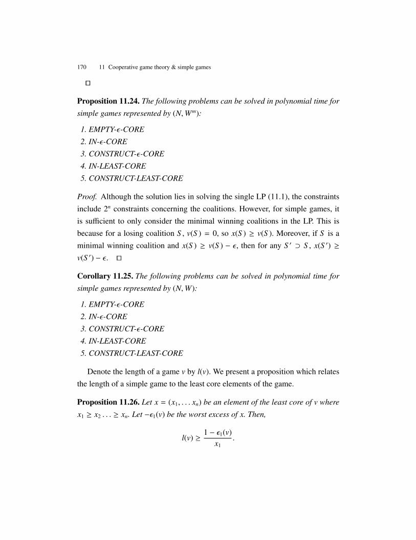
170 11 Cooperative game theory & simple games
ut
Proposition 11.24. The following problems can be solved in polynomial time for
simple games represented by (N,Wm):
1. EMPTY-ε-CORE
2. IN-ε-CORE
3. CONSTRUCT-ε-CORE
4. IN-LEAST-CORE
5. CONSTRUCT-LEAST-CORE
Proof. Although the solution lies in solving the single LP (11.1), the constraintsinclude 2n constraints concerning the coalitions. However, for simple games, itis sufficient to only consider the minimal winning coalitions in the LP. This isbecause for a losing coalition S , v(S ) = 0, so x(S ) ≥ v(S ). Moreover, if S is aminimal winning coalition and x(S ) ≥ v(S ) − ε, then for any S ′ ⊃ S , x(S ′) ≥v(S ′) − ε. ut
Corollary 11.25. The following problems can be solved in polynomial time for
simple games represented by (N,W):
1. EMPTY-ε-CORE
2. IN-ε-CORE
3. CONSTRUCT-ε-CORE
4. IN-LEAST-CORE
5. CONSTRUCT-LEAST-CORE
Denote the length of a game v by l(v). We present a proposition which relatesthe length of a simple game to the least core elements of the game.
Proposition 11.26. Let x = (x1, . . . xn) be an element of the least core of v where
x1 ≥ x2 . . . ≥ xn. Let −ε1(v) be the worst excess of x. Then,
l(v) ≥1 − ε1(v)
x1.

11.7 Least core 171
Proof. Let S be a winning coalition of length l(v). Since x(C) − v(C) ≥ −ε1(v)for all C ⊆ N, then x(S ) − 1 ≥ −ε1(v). This implies that there exists at least oneplayer i ∈ S such that xi ≥
1−ε1(v)l . Therefore, x1 ≥ xi ≥
1−ε1(v)l(v) . Thus,
l(v) ≥1 − ε1(v)
x1.
ut
For certain classes of simple games, the inequality in Proposition 11.26 turn outto be equalities. If v is singleton game, then l(v) =
1−ε1(v)x1
= 1. Similarly, if v is aunanimity game, l(v) =
1−ε1(v)x1
= n.
Proposition 11.27. If computing the length of a simple game (N, v) is NP-hard,
then IN-ε-CORE for (N, v) is NP-hard.
Proof. Consider the payoff x = (1n , . . . ,
1n ) for (N, v). Denote the length of (N, v)
by l(v). The payoff of the smallest winning coalition is l(v)n . The worst excess of
(N, v) for payoff x is l(v)n − 1.
The payoff x is in the ε-core if and only if l(v)n ≥ 1 − ε. If there is an oracle
to compute IN-ε-CORE in polynomial time, then by using different values of ε,binary search can be used to compute the l(v). Therefore computing l(v) reducesto solving IN-ε-CORE. Since l(v) is NP-hard to compute, IN-ε-CORE is NP-hard.ut
For many important simple coalitional games such as simple coalitional skillgames, threshold graph games and threshold network flow games, computing thelength is NP-hard [12]. Proposition 11.27 implies that if the length of a simplegame is NP-hard and unless P=NP, then there is no polynomial time separationoracle to solve the least core LP. This means that, if a polynomial time algorithmdoes exist, one needs to make extra use of the combinatorial structure of theunderlying game.
Let (N, v) be a simple game and x be any payoff of (N, v) we will denote1 − ε1(x, v) by δ1(x, v) and 1 − ε1(v) by δ1(v). The value δ1(x, v) is the payoff ofany coalition with the worst excess.

172 11 Cooperative game theory & simple games
Let (N, v) be a simple game and x be any payoff of (N, v). We will denote1 − ε1(x, v) by δ1(x, v) and 1 − ε1(v) by δ1(v). The value δ1(x, v) is the payoff ofany coalition with the worst excess.
Lemma 11.28. Let (N, v) be a simple game and x be any efficient payoff of (N, v).Consider the game (N ∪ {n + 1}, v′) which is obtained by adding a passer player
n + 1 to the game (N, v). For any efficient payoff x′ for (N ∪ {n + 1}, v′), if x′n+1 = a
and x′i = (1 − a)xi for i ∈ N, then
1. δ1(x′, v′) = Min(a, (1 − a)δ1(x, v)).2. If x′ is a least core payoff of (N ∪ {n + 1}, v′), then a = (1 − a)δ1(x, v) and
x′n+1(v′) = δ1(v′).
Proof. Since {n + 1} is a winning coalition, the worst excess of {n + 1} for payoff
x′ is a − 1 which implies that δ1(x′, v′) ≤ a.For S ⊆ N, any coalition S ∪ {n + 1} is not a minimal winning coalition.
Therefore, to examine other coalitions with the worst excess in (N ∪ {n + 1}, v′)for payoff x′, we look at subsets of N. The worst payoff for winning coalitionsamong N is then (1−a)δ1(x, v). This implies that δ1(x′, v′) ≤ (1−a)δ1(x, v). Sinceall subsets of N∪{n+1} have been considered, δ1(x′, v′) = Min(a, (1−a)δ1(x, v)).
We now prove that payoff x′ is a least core payoff of (N ∪ {n + 1}, v′), only ifa = (1 − a)δ1(x, v) and x′n+1(v′) = δ1(v′).
The value δ1(x′, v′) is maximized only when a = (1−a)δ1(x, v). Also, δ1(x′, v′)is maximum only when the optimum payoff δ1(v′) is given to player n + 1, i.e.,when x′n+1 = a = δ1(v′). ut
We define a representation of a simple game as passer-reasonable if, for anysimple game, the game with a newly added passer can also be represented andthere is at most polynomial blowup. WVGs, MWVGs, and coalitional skill gamesare examples of passer-reasonable representations.
Deng and Fang [58] note that “the most natural problem is how to efficiently
compute the value ε1 for a given cooperative game. The catch is that the com-
putation of ε1 requires one to solve a linear program with exponential number

11.8 Nucleolus 173
of constraints.” It is not clear that the least core worst excess can be computedefficiently even if a least core payoff is given. However, we have the followingresult.
Proposition 11.29. An oracle to compute a least core payoff for a simple game
in any passer-reasonable representation can be used to compute the worst excess
of a least core payoff.
Proof. Consider a game (N, v) in a passer-reasonable representation. Use the or-acle to compute x = (x1, . . . , xn), a least core payoff of (N, v).
Denote the worst excess (as yet unknown) of x by −ε1(v) and 1 − ε1(v) byδ1(v). Then, we know that δ1(x, v) = δ1(v). Form a new game (N ∪ {n + 1}, v′) byadding a passer player n + 1 to the game such that v′({n + 1}) = 1 and v′(S ) = 1if and and only if v(S ) = 1 for all S ⊆ N. Since (N, v) is in a passer-reasonablerepresentation, (N ∪ {n + 1}, v′) can also be represented by a passer-reasonablerepresentation.
Use the oracle to compute x′ = (x′1, . . . x′n+1), a least core payoff of (N ∪ {n +
1}, v′). From Lemma 11.28, we know that x′n+1(v′) = δ1(v′) and x′n+1 = (1 −x′n+1)δ1(x, v)). This means that,
x′n+1(v′)1 − x′n+1(v′)
= δ1(v) = 1 − ε1(v) (11.2)
From (11.2), we know that ε1(v) = 1 − δ1(v) can be computed by adding apasser to (N, v) to form game (N ∪ {n + 1}, v′) and then computing x′n+1(v′). ut
11.8 Nucleolus
Elkind et al. [68] showed that CONSTRUCT-NUCELULOS is NP-hard forWVGs. We check the complexity of CONSTRUCT-NUCLEOLUS for a simplegame represented by (N,W) and (N,Wm). It is well-known that the nucleolus isunique [189]. The nucleolus can be computed by solving a series of linear pro-grams [78]:

174 11 Cooperative game theory & simple games
Initially, 0 = {∅,N} and ε0 = 0. The value εr is the optimal value of LPr andr = {S ∈ 2N : x(S ) = v(S ) − εr for every x ∈ Xr} where Xr{x ∈ I(v) : (x, εr) is anoptimal solution of LPr}. Kopelowitz [122] showed that a maximum of n − 1 LPprogram iterations need to be run before one arrives at the solution x∗ which isthe nucleolus. The solution to LP1 is the least core of the game. Since, nucleolusis a least-core payoff, if computing the least core of a game is NP-hard, then itimplies that computing the nucleolus is NP-hard. The following is the descriptionof LPk in the series of LPs.
min εs.t. x(S ) = v(s) − εr , for all S ∈ r, r = 0, . . . , k − 1 ,
x(S ) ≥ v(S ) − ε , for all S ∈ 2N \⋃r=k−1
r=0 r,
x ∈ I(v) .
(11.3)
The nucleolus is a complex solution and no polynomial algorithm is knownfor computing the nucleolus in general. The computation of the nucleolus fordifferent cooperative games has attracted much attention [126]. Only for somespecial classes of cooperative game can the nucleolus be computed efficiently,for example, standard tree games [102], convex games [125], weighted votinggames with small weights [70] and assignment games [198]. Computing the nu-cleolus is NP-hard for min-cost spanning tree games [73], general flow gamesand linear production games [59]. We consider using the following meta-theoremto compute the nucleolus.
Theorem 11.30. (Elkind and Pasechnik: Theorem 5 in [70]) Given a coalitional
game G, suppose that we can, for any payoff vector p, identify the top n distinct
deficits under p, as well as the number of coalitions that have these deficits in
polynomial time. Then we can compute the nucleolus in polynomial time.
However, Theorem 11.30 cannot be used to compute the nucleolus for simplegames represented by minimal winning coalitions or winning coalitions. For ex-ample, if |W | is small enough, then computing the condition in Theorem 11.30reduces to a knapsack problem.

11.8 Nucleolus 175
If CONSTRUCT-NUCLEOLUS can be solved efficiently, this also meansthat IN-NUCLEOLUS can be solved efficiently by first computing the nucleo-lus and then comparing it with the payoff in consideration. This also implies thatCONSTRUCT-BARGAINING-SET and CONSTRUCT-KERNEL are easy. It iswell known that in a simple game, if a player is a dummy, it gets zero payoff notonly in the nucleolus but in every member of the kernel. We now give an exampleof a simple game where there are no vetoers and no dummies but still there is aplayer who gets zero nucleolus payoff:
Example 11.31. Let N = {1, 2, 3, 4}. Let
Wm(v) = {{1, 2}, {1, 3}, {2, 3, 4}}.
The game has no vetoer and no dummy. Let x = (x1, x2, x3, x4) be the nucleoluspayoff of the simple game v. From the relative powers of the players, we can seethat x1 ≥ x2 = x3 ≥ x4. Since the sum of the nucleolus payoffs of all playersis equal to one, x1 + 2x2 + x4 = 1. The two candidates for the value of the firstelement of the excess vector of x are (x1 + x2) − 1 and (2x2 + x4) − 1. For x to bethe nucleolus, the excess vector of x must lexicographically be the greatest. Thisis the case when (x1 + x2)− 1 = (2x2 + x4)− 1. This means that x2 = x3 = 1
3 −23 x4
and x1 = 13 + 1
3 x4. It is easy to work out that the excess vector of x is maximumwhen x4 = 0.
Peleg [175] proved that for certain WVGs, the nucleolus is simply equal to thenormalized weights of the players:
Proposition 11.32. (Peleg [175]) Consider a constant sum homogeneous weighted
voting game v = [q; w1, . . . ,wn] in which each dummy gets zero weight. Then the
nucleolus is equal to (w1/w(N), . . . ,wn/w(N)).
We use some examples and comments to clarify certain concepts which havenot always been used clearly in the game theory literature. For example, on page5 in [68], it is mentioned that Peleg’s proposition holds for any constant sumweighted voting games. This may not be true if the dummy players are not given

176 11 Cooperative game theory & simple games
zero weight. Moreover, in some places in the literature, Peleg’s proposition isassumed to hold for any homogeneous game. A homogeneous game does nothave to be constant sum: for example [2; 2, 2, 2]. Also, a homogeneous represen-tation can have a dummy with non-zero weight: for example [4, 2, 2, 1]. Proposi-tion 11.32 does not necessarily hold if all the conditions mentioned are not sat-isfied. The proposition says that there is at least one representation of a constantsum, homogeneous weighted voting game which coincides with the nucleolus.On the face of it, it seems that the proposition may provide an easy method tocompute a normalized WVG representation for a target nucleolus value. How-ever, for any nucleolus vector, it is not certain whether the nucleolus payoff isachievable. Moreover, even if the nucleolus payoff is feasible for some WVG, weneed to find a suitable quota which is the weight of all minimal winning coali-tions and the resultant WVG is constant-sum. The following example shows thatfinding a suitable quota may not be possible.
Example 11.33. Consider the target nucleolus (4/10, 3/10, 2/10, 1/10). Then theWVG in consideration is v = [q; 4, 3, 2, 1] where 6 ≤ q ≤ 10. However, forq = 6, 7, 8, 9, 10, it is easy to check that the following two conditions are not met:v is homogeneous and dummies get zero weight.
Definition 11.34. The nucleolus-like payoffs are those least core payoffs for
which the number of coalitions with the worst excess is minimum possible.
Proposition 11.35. For any monotone cooperative game (N, v) and nucleolus-
like payoff x, assume that there exists a player i such that for all S ∈ A1x(v), we
have that i ∈ S . Then, for player j other than i, either for all S ∈ A1x(v), j ∈ S or
we have that x j = 0.
Proof. Assume that there exists a coalition S ∈ A1x(v) such that player j < S . Let
δ = ε1−ε22 . Then if j donates δ amount of its payoff to i, this reduces the number of
−ε1-coalitions. This cannot be since x is nucleolus-like. ut
Proposition 11.36. For simple games represented by (N,Wm), CONSTRUCT-
PRENUCLEOLUS and CONSTRUCT-NUCLEOLUS can be solved in polynomial
time.

11.9 Kernel and bargaining set 177
Proof. It follows from Theorem 7 of [185] that, instead of examining 2n coali-tions, it is sufficient to examine a small collection of coalitions B to compute thenucleolus. The set B consists of MWCs plus certain other winning coalitions.From the definition of B in [185], it is easy to see that B ⊂ C where
C = Wm ∪ {S ∪ {i}|i ∈ N, S ∈ Wm}.
Therefore, the standard series of linear programs can be used to compute thenucleolus where in place of 2n coalitions, only |C| coalitions are considered. ut
This implies that for a simple game represented by (N,Wm), IN-PRENUCLEOLUSand IN-NUCLEOLUS can be solved in polynomial time and CONSTRUCT-PRENUCLEOLUS, CONSTRUCT-NUCLEOLUS, IN-PRENUCLEOLUS andIN-NUCLEOLUS can be solved in polynomial time for simple game representedby (N,W).
11.9 Kernel and bargaining set
In this section we examine the computational complexity of questions related tothe kernel and bargaining set of simple games. We also consider the prenucleolus.The relation between the kernel and prekernel is intricate. Maschler et al. [142]note that the kernel is not a subset of the prekernel. Prekernel does not have to beindividually rational so is not a subset of the kernel. However the intersection ofthe prekernel with the set of imputations is a subset of the kernel. Moreover, theparts of the kernel and the prekernel inside any ε-core always coincide [142]. Bothsolution concepts are closely related and an imputation that is in the prekernelis also an imputation of the kernel. However, the prekernel also contains payoffswhich are not imputations. For a non-zero-normalized simple game, a kernel maynot exist. In fact, the prekernel satisfies individual rationality on the class of zero-monotonic games.
If there are vetoers in a simple game, then the kernel of a simple game issimply a uniform distribution among the vetoers and no payoff for the vetoers [9].
178 11 Cooperative game theory & simple games
A naive algorithm to solve IN-KERNEL will take 2n(
n2
)time, as for each pair of
players, their maximum surpluses over each other are compared.
Proposition 11.37. For simple games represented by (N,Wm), IN-KERNEL and
IN-PREKERNEL can be solved in polynomial time.
Proof. Let x = (x1, . . . , xn) be a potential payoff. Then in order to check whetherx is in the kernel or the prekernel, it is sufficient to compute all the n(n − 1)surpluses: sv
i j(x) = max {v(S ) − x(S )|S ⊆ N \ { j}, i ∈ S }. One can compute svi j(x)
simply by examining MWCs which exclude j because for any MWC S and acoalition S ⊂ S ′, v(S ) − x(S ) = 1 − x(S ) ≤ 1 − x(S ′) = v(S ′) − x(S ′). A problemmay arise if it is the case that ∀S ∈ Wm, j ∈ S . Then we consider the singletoncoalition of i to compute sv
i j(x) because it gives the maximum surplus of −xi.Another problem may happen if ∀S ′ ∈ Wm such that j < S ′, we find that i < S ′.In that case, we consider the coalition S ′ which has the minimum x(S ). ThereforeS ′ ∪ { j} gives us sv
i j(x). ut
Corollary 11.38. For simple games represented by (N,W), IN-KERNEL and IN-
PREKERNEL can be solved in polynomial time.
Proposition 11.39. For simple games represented by (N,Wm), CONSTRUCT-
PREKERNEL and CONSTRUCT-KERNEL can be solved in polynomial time.
Proof. From [74], we know that an element in the so-called lexicographic prek-
ernel can be computed in polynomial time if the surpluses si j(x) correspondingto a given allocation x can be computed in polynomial time. From Prop 11.37,it then follows that an element in the lexicographic kernel can be computed inpolynomial time. Since the lexicographic prekernel is a subset of the intersectionof the prekernel and the least core, we can compute an element x in the prekernelof the (N,Wm). Moreover, as long as I(v) is non-empty, K(v) is non-empty andx is also in the kernel of (N,Wm), because the intersection of the kernel and theleast core coincides with the intersection of the prekernel and the least core forgames with non-empty I(v). ut
Corollary 11.40. The following statements follow from Proposition 11.39:
11.9 Kernel and bargaining set 179
1. For simple games represented by (N,W), CONSTRUCT-KERNEL and CONSTRUCT-
PREKERNEL can be solved in polynomial time.
2. For simple games represented by (N,Wm) and (N,W), CONSTRUCT-BARGAINING-
SET can be solved in polynomial time.
For simple games, if the core is non-empty, the bargaining set is equivalentto the core [65]. This means that for a game in which the core is non-empty,problems associated with the core are equivalent to problems associated with thebargaining set. For a unanimity game, any feasible imputation is in the bargainingset. This is because there is no scope for a valid objection. Let (N, v) be a simplegame with no passers. Then symmetric players get equal kernel payoff. Kernelpayoffs obey desirability relations, i.e., if i is more desirable than j, then xi ≥ x j.
If two players are symmetric, then they get equal payoff in the kernel andprekernel. However, if two players get equal payoff in the prekernel or kernel, itdoes not imply that the players are symmetric, even if the game is linear and hasno vetoers:
Example 11.41. Take WVG [5; 3, 2, 2, 1]. The imputation, (1/3, 1/3, 1/3, 0) is aprekernel imputation.
11.9.1 Wolsey’s theorem
Consider WVGs with non-increasing weights. A payoff vector x = (x1, . . . , xn)is homogeneous if each player receives either 0 or a fixed amount 1/r for somer ≤ n. Moreover, for set R = {1, . . . , r} ⊆ N,, we call the set T (R) = {1, . . . , k} ∪{r + 1, . . . , n}, the cover of R where k is the maximum with the property that∑
j∈T (R) w j < q. Then Wolsey claimed the following:
Claim. (Wolsey [217]) Let x = (x1, . . . , xn) be a homogeneous payoff in WVG[q; w1, . . . ,wn] where q ≥ w1 ≥ . . .wn. Then the payoff with xi = 1/r for i ∈ R
and xi = 0 for i ∈ N \ R is in the kernel if and only if
1. w(T (R)) + wr − wr+1 ≥ q and2. w(T (R)) − w1 + wk+1 + wr ≥ q.

180 11 Cooperative game theory & simple games
The paper has been cited in [124, 70, 68, 153]. The following counter exampleshows that at least the left to right implication does not hold in general.
Example 11.42. We consider the WVG v = [12; 8, 4, 2, 1]. The WVG v meets thecondition of the claim that q ≥ w1. This means that v({i}) = 0 for all i ∈ N. We seethat players 1 and 2 are vetoers. Player 1 is a vetoer because {2, 3, 4} is a losingcoalition as w({2, 3, 4}) = 7 < 12, and player 2 is a vetoer because {1, 3, 4} is alosing coalition as w({1, 3, 4}) = 11 < 12. Since players 1 and 2 are vetoers, thenucleolus payment of the game is (1/2, 1/2, 0, 0). Since the nucleolus is a memberof the kernel, the claim implies that both the conditions in the claim should besatisfied for r = 2.
We now consider the claim for the conditions that r = 2. If r = 2, then T (R) =
{1, 3, 4} with k = 1. Therefore w(T (R)) = 11. We consider the first condition.Since w(T (R)) + wr −wr+1 = 11 + 4− 2 = 13 > 12, the first condition is satisfied.However, the second condition is not satisfied: w(T (R)) − w1 + wk+1 + wr = 11 −8 + 4 + 4 = 11 6≥ 12.
From the proof in [217], it is evident that the case, when players i and j are ve-toers, is ignored in proving both left-to-right and right-to-left implications. There-fore, the required added condition for Wolsey’s theorem would be that there areno vetoers:
Theorem 11.43. Let x = (x1, . . . , xn) be a homogeneous payoff in WVG [q; w1, . . . ,wn]where there are no vetoers and q ≥ w1 ≥ . . .wn. Then the payoff with xi = 1/r for
i ∈ R and xi = 0 for i ∈ N \ R is in the kernel if and only if
1. w(T (R)) + wr − wr+1 ≥ q and
2. w(T (R)) − w1 + wk+1 + wr ≥ q.
11.10 Cost of stability
Unlike normal form games, where a mixed-strategy Nash equilibrium alwaysexists, coalitional games can be unstable if the core is empty. If the core of acoalitional game is empty, it is hard to ensure that players do not break off from

11.10 Cost of stability 181
the grand coalition to maximize their payoff. One recent proposal [23] to takecare of this problem is the idea of an external authority paying a supplemental
payment to incentivize the players to cooperate in a stable manner. This paymentis denoted by 4 and distributed in some way among the players. We use the samedefinitions as introduced in [23].
Definitions 11.44. For a given coalitional game G = (N, v), the adjusted coali-tional game G(4) = (N, v′) is obtained by setting v′(S ) = v(S ) for S ⊂ N and
v′(N) = v(N) + 4. Any payoff which is in the core of G(4) = (N, v′) is a super-imputation. The cost of stability (CoS) of a game is the minimum supplemental
payment CoS (G) such that G(CoS (G)) has a nonempty core.
If the core of a game is nonempty, then CoS is 0. It is easy to see that CoS (G)is the solution of the following LP:
min 4s.t. x(S ) ≥ v(S ) , for all S ⊂ N ,
xi ≥ 0 , for all i ∈ N,
x(N) = v(N) + 4 .
(11.4)
We now the consider the following natural computational problems related tothe cost of stability:Name: CoSInstance: Coalitional game (N, v)Question: Compute CoS
Name: SUPERIMPInstance: Coalitional game G = (N, v), supplement payment 4 and super-imputation (x1, . . . , xn) in G(4)Question: Is x ∈ CORE(G(4))?
It is known that solving CoS and SUPERIMP for WVGs is co-NP-hard [23].However, for other representations, the problems are tractable:

182 11 Cooperative game theory & simple games
Proposition 11.45. For a simple game represented by (N,Wm), solving SUPER-
IMP and CoS is in P.
Proof. The solution for both general problems seems to require considering 2n
constraints concerning the coalitions. However, for simple games, it is sufficientto consider only the minimal winning coalitions. This is because for a losingcoalition S , v(S ) = 0, so x(S ) ≥ v(S ). Moreover, if S is a minimal winningcoalition and x′(S ) ≥ v(S ), then for any S ′ ⊃ S , x′(S ′) ≥ v(S ′). ut
Propositions 11.46 draws the connection between the cost of stability and theleast core. The similarity in LP (11.1) for the least core and LP (11.4) leads us tothe following proposition:
Proposition 11.46. For a monotone cooperative game (N, v), if the separation
oracle O for a least core LP can be constructed and be solved in polynomial
time, then for (N, v), SUPERIMP and CoS are in P.
Proof. Consider payoff (x1, . . . , xn). Then oracle O, can check in polynomial timewhether x(S ) − v(S ) ≥ −ε for all S ⊂ N, or find a violated constraint otherwise.Then O can be used to solve SUPERIMP for (N, v). Also, O can be used as aseparation oracle to solve LP (11.4). ut
Corollary 11.47. Solving SUPERIMP and CoS are in P for the following games:
1. WVG with weight values polynomial in n,
2. Weighted matching games.
Proof. The separation oracle O for a least core LP can be constructed and solvedin polynomial time for WVG with weight values polynomial in n [68] andweighted matching games [118]. ut
Is it easy to notice the following relation between the cost of stability and theworst excess of an element in the least core: ε1(G) ≤ CoS (G) ≤ n(ε1(G)). Inorder to change G to a balanced G(4), we need to at least add ε1 amount to S 1
so that x′(S 1) ≥ 1. Therefore ε1 ≤ 4. Take an element x = (x1, . . . , xn) such that
11.11 Conclusion and open problems 183
x ∈ LC(G). Then x(S )− v(S ) ≥ −ε1. Consider x′ = (x′1, . . . x′n) where x′i = xi + ε1.
Take any coalition S ⊂ N. Then, x′(S ) − v(S ) = x(S ) + |S |ε1 − v(S ) ≥ 0.There may be multiple of ways of distributing the payoffs after the cost of
stability has been paid. We propose a natural and desirable solution for any coop-erative game called the super-nucleolus. The super-nucleolus is the nucleolus ofa cooperative game G if the core is nonempty and is the nucleolus of G(CoS (G))if the core of G is empty. Since the core of G(CoS (G)) is nonempty, it may beeasier to compute the super-nucleolus than the nucleolus of G in certain games.
11.11 Conclusion and open problems
One conclusion is that (N,Wm) is a comprehensive representation of simplegames which allows the efficient computation of almost all solutions. Similarly,Deng [58] states that, in all problems known, the concepts of the core, the bar-gaining set, and the stable set should be in increasing order of complexity. It willagain be useful to characterize this for any cooperative game. In this context, it isshown that computing the Shapley-Shubik index is at least as hard as computingthe Banzhaf index. It will be interesting to prove that for any representation of amonotone coalitional game, computing a least-core payoff has the same compu-tational complexity as computing the cost of stability. Another conjecture is thatif computing the length of a simple game is NP-hard, then computing a least corepayoff is NP-hard.

184 11 Cooperative game theory & simple games
Table 11.2. Complexity of cooperative game solutions in simple games
(N,W) (N,Wm) WVG MWVG
EMPTY-SHAPLEYVALUE always nonempty for any cooperative gameIN-SHAPLEYVALUE P ? NP-hard NP-hardCONSTRUCT-SHAPLEYVALUE P #P-complete #P-complete [60] #P-completeISZERO-SHAPLEYVALUE P P NP-hard NP-hard
EMPTY-CORE P P P [68] PIN-CORE P P P [68] PCONSTRUCT-CORE P P P [68] PISZERO-CORE P P P [68] P
EMPTY-ε-CORE P P NP-hard [68] NP-hardIN-ε-CORE P P NP-hard NP-hardCONSTRUCT-ε-CORE P P NP-hard NP-hardISZERO-ε-CORE N/A
EMPTY-LEAST-CORE always nonempty for any cooperative gameIN-LEAST-CORE P P NP-hard [68] NP-hardCONSTRUCT-LEAST-CORE P P NP-hard [68] NP-hardISZERO-LEAST-CORE N/A
EMPTY-NUCLEOLUS always nonempty if no passerIN-NUCLEOLUS P P ? ?CONSTRUCT-NUCLEOLUS P P NP-hard [68] NP-hardISZERO-NUCLEOLUS P P NP-hard [68] NP-hard
EMPTY-STABLE-SET always nonempty in simple gamesIN-STABLE-SET P P P PCONSTRUCT-STABLE-SET P P P PISZERO-STABLE-SET N/A
EMPTY-BARGAINING-SET always nonempty if no passerIN-BARGAINING-SET ? ? ? ?CONSTRUCT-BARGAINING-SET P P ? ?ISZERO-STABLE-SET N/A
EMPTY-KERNEL always nonempty if no passerIN-KERNEL P P ? ?CONSTRUCT-KERNEL P P ? ?ISZERO-KERNEL N/A
EMPTY-PREKERNEL always nonempty in any cooperative gameIN-PREKERNEL P P ? ?CONSTRUCT-PREKERNEL P P ? ?ISZERO-PREKERNEL N/A
EMPTY-PRENUCLEOLUS always nonempty in any cooperative gameIN-PRENUCLEOLUS P P ? ?CONSTRUCT-PRENUCLEOLUS P P NP-hard NP-hardISZERO-PRENUCLEOLUS P P NP-hard NP-hard
CORE-STABILITY P P P P
CoS P P coNP-hard [23] coNP-hardSUPERIMP P P coNP-complete [23] coNP-complete

12
Power indices of spanning connectivity games
The study of networks pervades all of science, from neurobiology to sta-
tistical physics.
- Steven Strogatz [199]
If the Internet is the next great subject for Theoretical Computer Science
to model and illuminate mathematically, then Game Theory, and Mathe-
matical Economics more generally, are likely to prove useful tools.
- Christos Papadimitriou [167]
Abstract We consider a simple coalitional game, called the spanning connectiv-ity game (SCG), based on an undirected, unweighted multigraph, where edgesare players. We examine the computational complexity of computing the votingpower indices of edges in the SCG. It is shown that computing Banzhaf valuesis #P-complete and computing Shapley-Shubik indices or values is NP-hard forSCGs. Interestingly, Holler indices and Deegan-Packel indices can be computedin polynomial time. Among other results, it is proved that Banzhaf indices can becomputed in polynomial time for graphs with bounded treewidth.
12.1 Introduction
In this chapter, we study the natural problem of computing the influence of edgesin keeping an unweighted and undirected multigraph connected. Game theorists

186 12 Power indices of spanning connectivity games
have studied notions of efficiency, fairness and stability extensively. Therefore, itis only natural that when applications in computer science and multiagent sys-tems require fair and stable allocations, social choice theory and cooperativegame theory provide appropriate foundations. For example, a network admin-istrator with limited resources to maintain the links in the network may decide tocommit resources to links according to their connecting ability. A spy networkcomprises communication channels. In order to intercept messages on the chan-nels, resources may be utilized according to the ability of a channel to connectall groups. In a social network, we may be interested in checking which connec-tions are more important in maintaining connectivity and hence contribute moreto social welfare.
Our model is based on undirected, unweighted and connected multigraphs.All the nodes are treated equally, and the importance of an edge is based solelyon its ability to connect all the nodes. Using undirected edges is a reasonableassumption in many cases. For example, in a social network, relations are usuallymutually formed.
We use a multigraph as a succinct representation of a simple coalitional gamecalled the spanning connectivity game (SCG). The players of the game are theedges of the multigraph. The importance of an edge is measured by computingits voting power index in the game.
The whole chapter is concerned with computing solutions for SCGs. In Sec-tion 12.2, a summary of related work is given. In Section 12.3, preliminarydefinitions related to graph theory and coalitional games are given, and we de-fine SCGs. Section 12.4 presents hardness results for computing Banzhaf val-ues and Shapley-Shubik indices. In Section 12.5, positive computational resultsfor Banzhaf values and Shapley-Shubik indices are provided for certain graphclasses. Section 12.6 presents a polynomial-time algorithm to compute Holler in-dices and Deegan-Packel indices. In Section 12.7, a summary of results is givenand future work is discussed.

12.3 Preliminaries 187
12.2 Related work
Power indices such as the Banzhaf and Shapley-Shubik indices have been usedto gauge the power of a player corporate networks [52]. These indices have re-cently been used in network flow games [24], where the edges in the graph havecapacities and the power index of an edge signifies the influence that an edgehas in enabling a flow from the source to the sink. Voting power indices havealso been examined in vertex connectivity games [27] on undirected, unweightedgraphs; there the players are nodes, which are partitioned into primary, standard,and backbone classes.
The study of cooperative games in combinatorial domains is widespread inoperations research [38, 54]. Spanning network games have been examined previ-ously [101, 210] but they are treated differently, with weighted graphs and nodes
as players (not edges, as here). The SCG is related to the all-terminal reliabil-ity model, a non-game-theoretic model that is relevant in broadcasting [209, 29].Whereas the reliability of a network concerns the overall probability of a networkbeing connected, this chapter concentrates on resource allocation to the edges.A game-theoretic approach can provide fair and stable outcomes in a strategicsetting. The hardness results in this chapter are a strengthening of the hardnessresults for the more general, min-base games, introduced in [155].
12.3 Preliminaries
12.3.1 Graph theory
Definition 12.1. A multigraph G = (V, E, s) consists of a simple underlying graph
(V, E) with a multiplicity function s : E 7→ N where N is the set of natural
numbers excluding 0. Let |V | = n and |E| = m. For every underlying edge i ∈ E,
we have si edges in the multigraph. The multigraph has a total of M =∑
i∈E si
edges and the set of all of these edges isM.
We note that G = (V, E, s) is a compact representation of multigraphs whichcan contain exponential number of parallel edges.

188 12 Power indices of spanning connectivity games
Definition 12.2. A subgraph G′ = (V ′,M′) of a graph G = (V,M) is a graph
where V ′ is a subset of V andM′ is a subset ofM in which case the vertex set of
M′ is a subset of V ′. A subgraph H is a connected spanning subgraph of a graph
G if it is connected and has the same vertex set as G.
12.3.2 Spanning connectivity game
For each connected multigraph (V, E, s) where si is the multiplicity of underly-ing edge i ∈ E, we define the SCG, spanning connectivity game, (M, v) with M
players (one player corresponding to each parallel edge) and valuation functionv, defined as follows for S ⊆ E:
v(S ) =
1, if there exists a spanning tree T = (V, E′) such that E′ ⊆ S
0, otherwise
It is easy to see that for a connected graph with more than one vertices, theSCG (M, v) is a simple game because the outcome is binary, v is monotone, v(∅) =
0 and v(E) = 1. We consider power indices and cooperative game solutions forthe edges in the SCG.
12.4 Complexity of computing power indices
We define the problems of computing the power indices of the edges in the SCG.For any power index X (e.g. Banzhaf value, Banzhaf index, Shapley-Shubik in-dex etc.) we define the problem SCG-X as follows:
Problem: SCG-XInstance: Multigraph G
Output: For the SCG corresponding to G, compute X for all the edges.
Computation of power indices of SCGs has relations with computation of reli-ability in networks. We will use these connections in some of our computational

12.4 Complexity of computing power indices 189
results. We will now present the prerequisite background of reliability compu-tation. We represent a communication network as a multigraph, where an edgerepresents a connection that may or may not work. An edge is said to be op-
erational if it works. For a given graph G, the reliability Rel(G, {pi}) of G is theprobability that the operational edges form a connected spanning subgraph, giventhat each edge is operational with probability pi for i = 1, . . .m.
Problem: Rational Reliability ProblemInstance: Multigraph G and pi ∈ Q for all i, 1 ≤ i ≤ m
Output: Compute Rel(G, {pi}).
A special case of the reliability problem is when every edge has the same prob-ability p of being operational. This is called the Functional Reliability Problem.
Definition 12.3. Let Ni be the number of connected spanning subgraphs with i
edges. Then the required output of the Functional Reliability Problem is the reli-ability polynomial
Rel(G, p) =
m∑i=0
Ni pi(1 − p)m−i.
Problem: Functional Reliability ProblemInstance: Multigraph G
Output: Compute the coefficients Ni of the reliability polynomial for all i,1 ≤ i ≤ m.
Ball [29] points out that an algorithm to solve the Rational Reliability Problemcan be used as a sub-routine to compute all the coefficients for the FunctionalReliability Problem. Moreover he proved that computing the general coefficientNi is NP-hard and therefore computing the rational reliability of a graph is NP-hard. As we will see in Section 12.5, reliability problems have connections withcomputing power indices of SCG. We first prove that SCG-BANZHAF-VALUEis #P-complete.

190 12 Power indices of spanning connectivity games
Proposition 12.4. SCG-BANZHAF-VALUE is #P-complete even for simple, bi-
partite and planar graphs.
Proof. We present a reduction from the problem of counting connected span-ning subgraphs. SCG-BANZHAF-VALUE is clearly in #P because a connectedspanning subgraph can be verified in polynomial time. It is known that countingthe total number of connected spanning subgraphs is #P-complete even for sim-ple, bipartite and planar graphs ( [28], p. 305). We now reduce the problem ofcomputing the total number of connected spanning subgraphs to solving SCG-BANZHAF-VALUE. Take G = (V, E) with n nodes and m edges. Transformgraph G into G′ = (V ∪ {n + 1}, E ∪ {m + 1}) by taking any node and connect-ing it to a new node via a new edge. Then the number of spanning subgraphsin G is equal to the Banzhaf value of edge m + 1 in graph G′. This shows thatSCG-BANZHAF-VALUE is #P-complete. ut
Similarly, SCG-SS is NP-hard.
Proposition 12.5. SCG-SS is #P-complete even for simple graphs.
Proof. The proof follows from Theorem 3.29. We demonstrate the application ofTheorem 3.29 by giving a complete proof. We show that computing the Shapley-Shubik indices is at least as hard as computing the total number of winning coali-tions. Let Ni be the number of connected spanning subgraphs of G with i edges.We know that computing Ni is NP-hard [29]. We show that if there is an algo-rithm polynomial in the number of edges to compute the Shapley-Shubik indexof all edges in the graph, then each Ni can be computed in polynomial time.
We obtain graph G0 by the following transformation: for some node v ∈ V(G),we link it by a new edge x to a new node vx. Then, by definition, the Shapley-Shubik value κx(G0) of player x is
∑mr=0 r!Nr(|E(G)| − r)! =
∑mr=0 r!N′r, where we
write N′r for Nr(m − r)!, for all r.Similarly we can construct Gi by adding a path Pi of length i to vx where Pi
has no edge or vertex intersection with G. Therefore
m∑r=0
(r + i)!N′r = κx(Gi). (12.1)

12.5 Polynomial time cases 191
For i = 0, . . . ,m, we get an equation of the form of (12.1) for each Gi. Theleft-hand side of the set of equations can be represented by an (m + 1) × (m + 1)matrix A where Ai j = (i + j − 2)!. The set of equations is independent because A
has a non-zero determinant of (1!2! · · ·m!)2 (see e.g. Theorem 1.1 [20]). If thereis a polynomial time algorithm to compute the Shapley-Shubik index of eachedge in a simple graph, then we can compute the right-hand side of each equationcorresponding to Gi.
The biggest possible number in the equation is less than (2m)! and can berepresented efficiently. The biggest possible number in the equation is less than(2m)! and can be represented efficiently. This follows from the fact that m! ≤mm and hence to represent (2m)!, one will use at most log2((2m)2m) = 2m(1 +
log2 m) ≤ 3m log2 m bits.We can use Gaussian elimination to solve the set of linear equations in O(m3)
time. Moreover, each number that occurs in the algorithm can also be stored in anumber of bits quadratic of the input size (Theorem 4.10 [123]). Therefore SCG-SS is NP-hard. ut
12.5 Polynomial time cases
In this section, we present polynomial time algorithms to compute voting powerindices for restricted graph classes including graphs with bounded treewidth. Wefirst consider the trivial case of a tree. If the graph G = (N, E) is a tree then there isa total of n− 1 edges and only the grand coalition of edges is a winning coalition.Therefore a tree is equivalent to a unanimity game. This means that each edgehas a Banzhaf index and Shapley-Shubik index of 1
n−1 . In the case of the sametree structure but with multiple parallel edges, we refer to this multigraph as apseudo-tree.
Proposition 12.6. Let G = (N, E, s) be a pseudo-tree such that the underlying
edges are 1, . . . ,m with multiplicities s1, . . . , sm. Then,

192 12 Power indices of spanning connectivity games
ηi1 =
m∏j=1j,i
(2s j − 1). (12.2)
Proof. Note that m = n − 1 in this case. Suppose edge i1 is a parallel edge cor-responding to edge i in the underlying graph. Edge i1 is critical for a coalition C
if the coalition C contains no edges parallel to i1 but contains at least one sub-edge corresponding to each edge other than i. The number of such coalitions is∏m
j=1j,i
(2s j − 1), which gives (12.2).
ut
Proposition 12.7. Let G = (N, E, s) be a pseudo-tree such that the underlying
edges are 1, . . . ,m with multiplicities s1, . . . , sm where s =∑m
i=1 si. Then the
Shapley-Shubik indices can be computed in time polynomial in the total number
of edges and number of players.
Proof. Denote by er the coefficient of xr in
∏1≤ j≤n−1
j,i
((1 + x)s j − 1).
Then er is the number of coalitions with r edges which include at least oneparallel edge for each underlying edge j except i. Denote by ik the kth paralleledge of underlying edge i ∈ E. Then, by definition of the Shapley-Shubik value,for 1 ≤ k ≤ si,
κik(G) =
s−si∑r=n−2
err!(s − r − si)!.
Assume that the total number of edges s is polynomial in input size. Then eachof the values si are also polynomial in the input size. In that case, the generatingfunction can be expanded in polynomial time and the Shapley-Shubik indices canbe computed. ut
We now consider graphs with bounded treewidth. Note that trees and pseudo-trees have treewidth 1.

12.5 Polynomial time cases 193
Definition 12.8. For a graph G = (V, E), a tree decomposition is a pair (X,T ),where X = {X1, ..., Xn} with X j ⊂ 2V for 1 ≤ j ≤ n, and T is a tree whose nodes
are the subsets Xi with the following properties:
1.⋃
1≤i≤n Xi = V
2. For every edge (v,w) ∈ E, there is a subset Xi that contains both v and w.
3. If Xi and X j both contain a vertex v, then all nodes Xz of the tree in the path
between Xi and X j also contain v.
The width of a tree decomposition is the size of its largest set Xi minus one.
The treewidth tw(G) of a graph G is the minimum width among all possible tree
decompositions of G.
Proposition 12.9. If the reliability polynomial defined in Definition 12.3 can be
computed in polynomial time, then the following problems can be computed in
time polynomial in the number of edges:
1. the number of connected spanning subgraphs;
2. the Banzhaf indices of edges.
Proof. We deal with each case separately.
1. By definition, Ni is the number of connected spanning subgraphs with i edges.The value Ni is also present as a coefficient in the reliability polynomial. If allcoefficients Ni are computable in polynomial time, then the total number ofconnected spanning subgraphs
∑mi=0 Ni is computable in polynomial time.
2. We know that ηi(G) = 2ωi(G) − ω(G) (see Lemma 3.27) where ω(G) is equalto the total number of winning coalitions and ωi(G) is the number of winningcoalitions including player i. Consider the graph G where the probability ofedge i being operational is set to 1 whereas the probability of other edges be-ing operational is set to 0.5. Then the reliability of the graph being connectedis equal to the ratio of the number of connected spanning subgraphs that in-clude edge i to 2M−1, the total number of subgraphs that include i. Therefore,ωi(v) the number of connected spanning subgraphs including edge i can becomputed in polynomial time too. ut
194 12 Power indices of spanning connectivity games
Corollary 12.10. Banzhaf indices of edges can be computed in polynomial time
for graphs with bounded treewidth.
Proof. This follows from the polynomial time algorithm to compute the reliabil-ity of a graph with treewidth k for some fixed k [7]. ut
Definition 12.11. Let G = (V, E) be a graph with source s and sink t. Then G is
a series-parallel graph if it may be reduced to K2 by a sequence of the following
operations:
1. replacement of a pair of parallel edges by a single edge that connects their
common endpoints;
2. replacement of a pair of edges incident to a vertex of degree 2 other than s or
t by a single edge so that 2 degree vertices get removed.
Graphs with bounded treewidth can be recognized in polynomial time [6].Series-parallel graphs are well-known classes of graphs with constant treewidth.Other graph classes with bounded treewidth are cactus graphs and outer-planargraphs. We see that whereas computing Banzhaf values of edges in general SCGsis NP-hard, important graph classes can be recognized and their Banzhaf valuescomputed in polynomial time.
When edges have special properties, their power indices may be easier to com-pute. We define a bridge in a connected graph to be an edge whose removal resultsin the graph being disconnected. A graph class is hereditary if for every graph inthe class, every subgraph is also in the class.
Proposition 12.12. If graph G belongs to a hereditary graph class, for which the
reliability polynomial of a graph can be computed in polynomial time, then the
Shapley-Shubik index of a bridge can be computed in time polynomial in the total
number of edges.
Proof. Let G = (V, E) be a graph where edge k is a bridge which connects twocomponents A = (VA, EA) and B = (VB, EB). Then |E| = |EA| + |EB| + 1. Ifthe reliability polynomial of G can be computed in polynomial time, then the

12.5 Polynomial time cases 195
reliability polynomial for each of the components A and B can be computed.Denote by Ni(A) and Ni(B) the number of connected spanning subgraphs in A andB respectively. These values are also the coefficients in the reliability polynomialof A and B respectively. Then the Shapley-Shubik index of player k is:
φk(G) =
∑|EA |
i=|VA |−1
∑|EB|
j=|VB|−1 Ni(A)N j(B)(i + j)!(|EA| + |EB| − i − j)!
|E|!.
ut
Our next result is that if the reliability of a simple graph can be computedthen the Banzhaf indices of the corresponding multigraph can be computed. Anaive approach would be to compute the Banzhaf values of each edge in a simplegraph and then, for the corresponding parallel edges in the multigraph, divide theBanzhaf value of the overall edge by the number of parallel edges. However, asthe following example shows, this approach is incorrect:
Example 12.13. Let G = (V, E, s) be the multigraph in Figure 12.1. Then, η41(vG) =
10, η11(vG) = 14, and η2(vG) = η3(vG) = 28. Therefore β41(vG) = 103×10+2×14+28+28 =
557 . Moreover, β11(vG) = 7
57 and β2(vG) = β3(vG) = 1457 . If we examine the underly-
ing graph of G′ in Figure 12.1, then η4(v′G) = 4 and η1(v′G) = η2(v′G) = η3(v′G) = 2giving β4(G′) = 2/5 and βi(G′) = 1/5 for i = 1, 2, 3. Therefore, the Banzhafvalues of edges in the underlying graph do not seem to give any direct way ofcomputing the Banzhaf values in the multigraph.
Fig. 12.1. Multigraph and its underlying graph
196 12 Power indices of spanning connectivity games
Lemma 12.14. If there is an algorithm to compute the reliability of the underly-
ing simple graph, then the algorithm can be used to compute the reliability of the
corresponding multigraph.
Proof. Let G = (V, E, s) be a multigraph in which there are si parallel edgesi1, . . . , isi corresponding to edge i. Let pi j be the probability that the jth paralleledge of edge i is operational. In that case Rel(G, p) is equal to Rel(G′, p′), whereG′ is the corresponding simple graph of G and the probability pi that edge i isoperational is 1 −
∏sij=1(1 − pi j). ut
We now prove in Proposition 12.15 that if there is an algorithm to computethe reliability of the underlying simple graph G, then it can be used to com-pute the Banzhaf indices of the edges in the corresponding multigraph of G. Itwould appear that the proposition follows directly from Lemma 12.14 and Propo-sition 12.9. However, one needs to be careful that the reliability computed is thereliability of the overall graph. Example 12.13 shows that computing the Banzhafvalues of the edges in the underlying simple graph does not directly provide theBanzhaf values of the parallel edges in the corresponding graph.
Proposition 12.15. For a multigraph G and edge i, let G′ be the multigraph where
all the other edges parallel to edge i are deleted. Then if the reliability of G′ can
be computed in polynomial time, then the Banzhaf value of edge i in G can be
computed directly by analysing G′.
Proof. Recall that G is a multigraph with a total of M edges. Given an algorithmto compute the reliability of G′, we provide an algorithm to compute the Banzhafvalues of the parallel edges of edge i in G. For graph G′, set the operational proba-bilities of all edges to 0.5 except i which has an operation probability of 1− 0.5si .and compute the overall reliability r(G′) of the graph. Then, by Lemma 12.14,ω(G) is 2Mr(G′).
Now for G′, set the operational probabilities of all edges to 0.5 except i whichhas an operation probability of 1. Let the reliability of G′ with the new prob-abilities be r′(G′). We see that r′(G′) is equal to ωi(G′)/2M−si . Then ωi(G) =
12.7 Conclusion 197
2si−1ωi(G′) = 2M−1r′(G′). The Banzhaf value of i is then 2ωi(G) − ω(G). A simi-lar approach gives Banzhaf values of the other edges, from which all the Banzhafindices can be computed. ut
12.6 Other power indices
We also consider the complexity of computing the Holler indices and Deegan-Packel indices and find that they can be computed in polynomial time.
Proposition 12.16. For SCGs corresponding to multigraphs, Holler indices and
Deegan-Packel indices can be computed in polynomial time.
Proof. We use the fact that the number of trees in a multigraph can be computedin polynomial time, which follows from Kirchhoff’s matrix tree theorem [99].Given a connected graph G with n vertices, let λ1, λ2, ..., λn−1 be the non-zeroeigenvalues of the Laplacian matrix of G (the Laplacian matrix is the differenceof the degree matrix and the adjacency matrix of the graph). Kirchhoff provedthat the number of spanning trees of G is equal to any cofactor of the Laplacianmatrix of G [99]: t(G) = 1
nλ1λ2 · · · λn−1. So now that we have a polynomial-timemethod to compute the number of spanning trees t(G) of graph G, we claim thisis sufficient to compute the Holler values of the edges. If an edge i is a bridge,then it is present in every spanning tree and its Holler value is simply the totalnumber of spanning trees. If i is not a bridge then |Mi| = t(G)− t(G\e). Moreover,since the size of every minimal winning coalition is the same, namely (n− 1), theHoller indices and Deegan-Packel indices coincide for an SCG. ut
12.7 Conclusion
This chapter examined fairness-based cooperative game solutions of SCGs, forallocating resources to edges. We looked at the exact computation of power in-dices. In [22], an optimal randomized algorithm to compute Banzhaf indices andShapley-Shubik indices with the required confidence interval and accuracy is pre-sented. Since the analysis in [22] is not limited to a specific representation of a

198 12 Power indices of spanning connectivity games
coalitional game, it can be used to approximate Banzhaf indices and Shapley-Shubik indices in SCGs.
The results of the chapter are summarized in Table 12.1. This framework canbe extended to give an ordering on the importance of nodes in the graph [40]. Toconvert a resource allocation to edges to one on nodes, the payoff for an edge isdivided equally between its two adjacent nodes. The total payoff of a node is thesum of the payoffs it gets from all its adjacent edges. This gives a way to quantifyand compare the centrality or connecting role of each node. It will be interestingto understand the properties of such orderings, especially for unique cooperativesolution concepts such as the nucleolus, Shapley-Shubik and Banzhaf indices.
The complexity of computing the Shapley-Shubik index for an SCG with agraph of bounded treewidth is open. If this problem is NP-hard, it will answer thequestion posed in the conclusion of [22] on whether there are any domains wherecomputing one of the Banzhaf index and Shapley-Shubik index is easy, whereascomputing the other is hard.
Table 12.1. Complexity of SCGs
Problem Input Complexity
SCG-BANZHAF-VALUE Simple, bipartite, planar graph #P-completeSCG-BANZHAF-INDEX Simple graph ?SCG-BANZHAF-(VALUE/INDEX) Multigraph with bounded treewidth PSCG-SS Multigraph #P-completeSCG-SS Multigraph with bounded treewidth ?SCG-H-(VALUE/INDEX) Multigraph PSCG-DP-(VALUE/INDEX) Multigraph P
13
Nucleolus of spanning connectivity games
The earth to be spann’d, connected by network,
The races, neighbors, to marry and be given in marriage,
The oceans to be cross’d, the distant brought near,
The lands to be welded together.
- Walt Whitman (Passage to India)
Two hold a garment; both claim it all. Then the one is awarded half, the
other half. Two hold a garment; one claims it all, the other claims half.
Then the one is awarded 3/4, the other 1/4.
- Talmud
Abstract We consider the least core imputations and the nucleolus of the span-ning connectivity game. For any least core imputation, we refer to the value of thespanning connectivity game as the payoff of any coalition with the worst(minimum)excess. We show that the value is equal to the reciprocal of the strength of the un-derlying graph.
We efficiently compute a unique partition of the edges of the graph, called theprime-partition, and find the set of coalitions which always get the worst excessfor every least core imputation. We define a partial order on the elements of theprime-partition which allows us to compute the nucleolus in polynomial time.
We also consider the problem of maximizing the probability of hitting a strate-gically chosen hidden network by placing a wiretap on a single link of a commu-nication network. This can be seen as a two-player win-lose (zero-sum) game that

200 13 Nucleolus of spanning connectivity games
we call the wiretap game. The nucleolus turns out be the unique maxmin strategywhich satisfies certain desirable properties.
13.1 Introduction
In the previous chapter, it was seen that computing Banzhaf values and Shapley-Shubik indices of an SCG are #P-complete. In this chapter, we will outline apolynomial time algorithm to compute the nucleolus of the SCG. The analysis isrestricted to unweighted simple graphs. However, all the results extend to multi-graphs. It is easy to see that any preimputation of a SCG is also an imputationsince there can be no edge e such that v(e) = 1 unless it is the only edge in thegraph.
For any least core imputation, we refer to the value of the SCG as the payoff
of any coalition with the worst excess. Therefore the value of the SCG G is equalto 1 − ε1(G) where −ε1 is the worst excess of a least core imputation of the SCG.We show that the value of the SCG is equal to the reciprocal of the strength ofthe underlying graph, a concept introduced by Gusfield [103].
We efficiently compute a unique partition of the edges of the graph, calledthe prime-partition. We find the set of coalitions which get the worst excess forany least core imputation. Using these special coalitions, which we call omni-
connected-spanning-subgraphs, we define a partial order on the elements of theprime-partition. Our definition in terms of omni-connected-spanning-subgraphsis central to proving our results.
From the partial order, we obtain a linear number of simple two-variable in-equalities that define the least-core-polytope. In contrast, the natural descriptionof the least-core-polytope is as the solutions to a linear program with exponen-tially many constraints. Our definition of the partial order allows us to find allleast core imputations that minimize the number of coalitions with the worst ex-cess.
Among these imputations, we efficiently compute the unique least core im-putation that maximizes the second worst excess. Hence, this imputation is the

13.3 Least core of SCGs 201
nucleolus of the game. The nucleolus turns out be a highly desirable maxminstrategy of the wiretap game (which is defined in Section 13.8).
13.2 Related work
The strength of an unweighted graph, which has a central role in our work,is also called the edge-toughness, and relates to the classical work of Nash-Williams [157] and Tutte [207]. Cunningham [53] generalized the concept ofstrength to edge-weighted graphs and proposed a strongly polynomial-time algo-rithm to compute it. Computing the strength of a graph is a special type of ratiooptimization in the field of submodular function minimization [93]. Cunning-ham used the strength of a graph to address two different one-player optimiza-tion problems: the optimal attack and reinforcement of a network. The prime-partition we use is a truncated version of the principal-partition, first introducedby Narayanan [156] and Tomizawa [205]. The principal-partition was used in anextension of Cunningham’s work to an online setting [172].
In many cases the nucleolus is hard to compute. The computational complex-ity of computing the nucleolus has attracted much attention [126], with both neg-ative results [68, 73, 59], and positive results [102, 70, 125, 198].
13.3 Least core of SCGs
Denote the set of spanning subgraphs of G by S. For a graph G, the value of theSCG val(G) is defined by the least-core payoff of any coalition with the worstexcess. Thus val(G) = 1 − ε1(G). It is easy to see that least core payoffs are thesolutions {x ∈ I(E) |
∑e∈S xe ≥ val(G) for all S ∈ S} to the following linear
program, which has the optimal value val(G).
max z
s.t.∑
e∈S xe ≥ z for all S ∈ S ,
x ∈ I(G) .
(13.1)

202 13 Nucleolus of spanning connectivity games
The following simple observation shows the importance of minimum con-nected spanning graphs in the analysis of the SCG. We denote by Gx the edge-weighted graph comprising the graph G with edge weights x(e) for all e ∈ E. Letw∗(x) be the weight of a minimum connected spanning graph of Gx.
Fact 1 The set of coalitions with the worst excess for imputation x is
{S ∈ S |∑e∈S
xe = w∗(x)} .
Proposition 13.1. An element of the least core of an SCG can be found in poly-
nomial time.
Proof. The size of the linear program (13.1) is exponential in the size of thegraph G, with an inequality for every subset of edges. However, this linear pro-gram can be solved using the ellipsoid method and a separation oracle, whichverifies in polynomial time whether a solution is feasible or returns a violatedconstraint [190]. For a candidate solution x = (x1, . . . , x|E|), we find in polynomialtime the minimum spanning tree T of the graph Gx. Use Kruskal’s algorithm tocompute the minimum spanning tree T of graph Gx. If we have x(E(T ))−1 ≥ −ε,then x is feasible. Otherwise, the constraint e(x,T ) ≥ −ε is violated. ut
The same separation oracle idea can be used to prove the following proposi-tion:
Proposition 13.2. For a SCG, solving SUPERIMP and CoS is in P.
Proof. Assume that the graph G has no bridges, because if there are bridges, thenthe bridge acts as a vetoer and the core is non-empty. We consider a superimputa-tion (x1, . . . , x|E|) such that x(E) = 1+4. For a candidate solution x = (x1, . . . , x|E|),we find in polynomial time the minimum spanning tree T of the graph Gx. Ifx(T ) ≥ 1, then x(S ) ≥ 1 for all S ⊂ E and x is a superimputation. If x(T ) < 1,then x is not a superimputation.
The size of the linear program (11.4) is exponential in the size of the graph G,with an inequality for every subset of edges. Again, this linear program can be

13.4 Cut-rate 203
solved using the ellipsoid method and a separation oracle, which verifies in poly-nomial time whether a solution is feasible or returns a violated constraint [190].We see that our solution to SUPERIMP for an SCG provides a separation oracleto solve CoS for the same SCG. ut
We will see in this chapter that not only is there a combinatorial method tocompute a least core imputation of a SCG in polynomial time but we also presenta way to compute the nucleolus in polynomial time.
13.4 Cut-rate
In this section, we show that for any least core imputation of the SCG, the pay-off of any coalition with the worst excess is equal to the cut-rate of the graph(Theorem 13.13). The cut-rate which is a property of a graph will be defined laterin Definition 13.5. The section does not present algorithmic results but the in-sights and tools from this section will be used in the latter sections to devise acombinatorial algorithm to compute the nucleolus of the SCG.
We start with the basic notations and definitions. From here on we fix a con-nected graph G = (V, E). Unless mentioned explicitly otherwise, any implicitreference to a graph is to G and α is an edge-imputation, which is a probabil-ity distribution on the edges E. For ease, we often refer to the weighted graph Gα
simply by α, where this usage is unambiguous. For a subgraph H of G, we denoteby α(H) the sum
∑e∈E(H) α(e), where E(H) is the edge set of H.
Definition 13.3. For every edge-imputation α, we denote its distinct weights by
xα1 > . . . > xαm ≥ 0 and define E(α) = {Eα1 , . . . , E
αm} such that Eα
i = {e ∈ E | α(e) =
xαi } for i = 1, . . . ,m.
Our initial goal is to characterize those partitions E(α) that can arise fromleast-core-imputations α. We start with the following simple setting. Assume thatthe prospective imputation is restricted to α such that |E(α)| = 2, and xα2 = 0.Thus, the imputation’s only freedom is the choice of the set Eα
1 . This is doneas a warm up exercise to highlight the importance of the cut-rate and minimum

204 13 Nucleolus of spanning connectivity games
spanning subgraphs in our analysis later on. In general an imputation may containdistinct payoff for all players.
By Fact 1, a coalition with the worst excess for α is a minimum connectedspanning subgraph H of α. So in order to maximize the worst excess, Eα
1 shouldbe chosen so as to maximize α(H). How can such an Eα
1 be found? To answer, werelate the weight of a minimum connected spanning subgraph H of α to Eα
1 .To determine α(H), we may assume about H that for every connected com-
ponent C of (V, E \ Eα1 ) we have E(H) contains E(C), since α(e) = 0 for every
e ∈ E(C). We can also assume that |Eα1 ∩ E(H)| is the number of connected com-
ponents in (V, E \ Eα1 ) minus 1, since this is the minimum number of edges in
E(H) that a connected spanning subgraph may have. To formalize this we use thefollowing notation.
Definition 13.4. Let E′ ⊆ E. We set CG(E′), to be the number of connected com-
ponents in the graph G \ E′, where G \ E′ is a shorthand for (V, E \ E′). If E′ = ∅
we just write CG.
Using the above notation, a connected spanning subgraph H is a minimumconnected spanning subgraph of α if |H∩Eα
1 | = CG(Eα1 )−CG = CG(Eα
1 )−1. Nowwe can compute α(H). By definition, xα1 = 1
|Eα1 |
and xα2 = 0 and therefore
α(H) =CG(Eα
1 ) −CG
|Eα1 |
.
We call this ratio that determines α(H) the cut-rate of Eα1 . Note that it uniquely
determines the weight of a minimum connected spanning subgraph of α.
Definition 13.5. Let E′ ⊆ E. The cut-rate of E′ in G is denoted by crG(E′) and
defined as follows.
crG(E′) B
CG(E′)−CG|E′ | if |V | > 1 and |E′| > 0 ,
0 otherwise .(13.2)
We write cr(E′), except to make a point of referring to a different graph.
13.4 Cut-rate 205
Thus, when |E(α)| = 2 and xα2 = 0, a best choice of Eα1 is one for which cr(Eα
1 )is maximum. Since E is finite, an Eα
1 that maximizes cr(Eα1 ) exists. If we can find
such a set Eα1 , we distribute the payoff 1 uniformly over Eα
1 to get the best possibleworst excess among homogeneous imputations.
Definition 13.6. The cut-rate of G is defined as opt B maxE′⊆E cr(E′) .
By opt, we always refer to the cut-rate of the graph G. In case we refer tothe cut-rate of some other graph, we add the name of the graph as a subscript.The value opt is a well known and studied attribute of a graph. It is equal to thereciprocal of the strength of a graph, as defined by Gusfield [103] and namedby Cunningham [53]. There exists a combinatorial algorithm for computing thestrength, and hence opt, that runs in time polynomial in the size of the graph, bywhich we always mean |V | + |E|.
We generalize the above technique to the case that α is not restricted. Assumeagain that H is a minimum connected spanning subgraph of α. Intuitively, evenif α has more than 2 distinct weights we would expect |Eα
1 ∩ E(H)| to be as smallas possible, i.e., CG(Eα
1 ) −CG. We would also expect |(Eα1 ∪ Eα
2 ) ∩ E(H)| to be assmall as possible, i.e., CG(Eα
1 ∪ Eα2 ) − CG. If these both hold then |Eα
2 ∩ E(H)| =CG(Eα
1 ∪ Eα2 ) − CG(Eα
1 ), which is the increase in the number of components weget by removing the edges of Eα
2 from G \ Eα1 . Thus, the total weight contributed
to H by edges in E(H) ∩ E(Eα2 ) is xα2 (CG(Eα
1 ∪ Eα2 ) − CG(Eα
1 )). Now, unlike theprevious case, we do not know xα2 . However, this is not a problem since, as weshall see, we are interested in the ratio
α(E(H) ∩ Eα2 )
α(Eα2 )
=CG(Eα
1 ∪ Eα2 ) −CG(Eα
1 )|Eα
2 |.
We use the following notation to express this and its extension to more weights.
Definition 13.7. For ` = 1, . . . , |E(α)| we set
crα` =CG(∪`i=1Eα
i ) −CG(∪`−1i=1 Eα
i )|Eα
` |.

206 13 Nucleolus of spanning connectivity games
The intuition above indeed holds, as stated in the following proposition.
Proposition 13.8. Let H be a minimum connected spanning subgraph of α. Then
|E(H) ∩ Eα` | = |E
α` |crα` for every ` such that xα` > 0.
Proof. Let H be a minimum connected spanning subgraph of α. And let t bethe maximum such that xαt > 0. We next show that |E(H) ∩ Eα
i | = |Eαi |crαi for
i = 1, . . . , t.Assume for the sake of contradiction that this is not so. Let k be minimal such
that |E(H) ∩ Eαk | , |E
αk |crαk . By the minimality of k we have
|E(H) ∩ (∪k−1i=1 Eα
i )| =k−1∑i=1
|Eαi |crαi . (13.3)
Set E′ = ∪ki=1Ek
i . By the definition of cut-rate the number of connected compo-nents in G \ E′ is
CG(E′) = 1 +
k∑i=1
|Eαi |crαi . (13.4)
Thus |E(H) ∩ E′| is at least∑k
i=1 |Eαi |crαi and therefore by (13.3) we have |E(H) ∩
Eαk | ≥ |E
αk |crαk .
Assume |E(H) ∩ Eαk | > |E
αk |crαk . Then, by (13.3), we have
|E(H) ∩ E′| >k∑
i=1
|Eαi |crαi . (13.5)
We show next that this implies that there exists a connected spanning subgraphwhose weight by α is strictly less than α(H) in contradiction to H being a min-imum connected spanning subgraph. Set s = CG(E′) and let C1, . . . ,Cs be theconnected components of G \ E′. Now as H is a minimum connected spanningsubgraph the set of edges in E(H)∩E′ does not have a cycle, otherwise we couldhave removed one of them to get a connected spanning subgraph with strictly lessweight. Thus the number of connected components of E(H)\E′ is 1+ |E∩E(H)|.Set r = |E′ ∩ E(H)| and let H1, . . . ,Hr be the connected components of H \ E′.

13.4 Cut-rate 207
Note that for each i ∈ {1, . . . , r} there exists a unique j ∈ {1, . . . , s} such thatE(Hi) ⊆ E(C j). For each j ∈ {1, . . . , s} set I j to be the set of all i ∈ {1, . . . , r}such that E(Hi) ⊆ E(C j). By (13.4) and (13.5) we have s < r and therefore by thepigeon-hole principle there exists j ∈ {1, . . . , r} such that |I j| > 1. Since C j is aconnected component and H a connected spanning subgraph there exist x, y ∈ I j
and e = {u, v} ∈ E(C j) \ ∪|I j |
i=1E(Hi) such that u ∈ V(Hx) and v ∈ V(Hy). Againbecause H is a connected spanning subgraph there is a path in H between u andv this path contains edges not in E(C j) because u, v are in different connectedcomponents of H \ E′. Thus this path contains an edge e′ ∈ E′ because onlyedges from E′ connect the vertices of C j to the rest of the graph. Consequently(H\{e′})∪{e} is a connected spanning subgraph. Since e < E′ we have α(e) < α(e′)and consequently α(H) > α((H \ {e′}) ∪ {e}). ut
Using Proposition 13.8 we can relate the weight of a minimum connectedspanning subgraph of α to the sets of E(α). This relationship also characterizesthe least-core-imputations, which are the edge-imputations whose minimum con-nected spanning subgraph weight is the maximum possible. The characterizationis stated in Theorem 13.13. However, before we prove Theorem 13.13, we needthe help of useful facts and propositions.
Fact 2 Let H be a minimum connected spanning subgraph of α and m = E(α)then α(H) =
∑mi=1 xαi |E
αi |crαi and for each i = 1, . . . ,m if crαi < 1 then there exists
e ∈ Eαi \ E(H).
Proof. By definition |E(H)| =∑m
i=1 |E(H)∩Eαi |. Therefore α(H) =
∑mi=1 xαi |E(H)∩
Eαi |. By applying Proposition 13.8 we get that α(H) =
∑mi=1 xαi |E
αi |crαi .
Fix i ∈ {1, . . . ,m}. By Proposition 13.8 we have |E(H) ∩ Eαi | = |Eα
i |crαi andhence if crαi < 1 then |E(H) ∩ Eα
i | < |Eαi | and therefore Eα
i \ E(H) is not empty.ut
Fact 3 Let E1, . . . , Es ⊆ E be such that Ei ∩ E j = ∅ for every distinct i, j ∈
{1, . . . , s}. For ` = 1, . . . , s let r` be the cut-rate of E` in G \ ∪`−1i=1 E`. Assume that
r` ≥ y (r` ≤ y) for each ` = 1, . . . , s. Then if there exists i ∈ {1, . . . , s} such that
ri > y (ri < y) we have cr(∪si=1Ei) > y (r < y) and otherwise cr(∪s
i=1Ei) = y.

208 13 Nucleolus of spanning connectivity games
Proof. By the definition of cut-rate CG(∪si=1Ei) = CG +
∑si=1 ri|Ei| and hence
cr(∪si=1Ei) =
(CG +∑s
i=1 xi|Ei|) −CG∑sj=1 |E j|
≥
∑si=1 y|Ei|∑sj=1 |E j|
= y.
Note that the above inequality is strict unless ri = y for i = 1, . . . , s. The proof forthe case that ri ≤ y for i = 1, . . . , s, is the same. ut
Lemma 13.9. If we have E1, E2 ⊆ E and E1 ∩ E2 = ∅ then
CG(E1 ∪ E2) ≥ CG(E1) + CG(E2) −CG (13.6)
Proof. We prove the statement by induction. Where there is no ambiguity, wewill sometimes refer to CG(E1) also as the components of the graph G when E1
is deleted from G.. If CG(E1) + CG(E2) = 2CG then (13.6) holds. Assume as aninductive hypothesis, that (13.6) holds when CG(E1) + CG(E2) = k > 2CG. Weshow that (13.6) holds for CG(E1) + CG(E2) = k + 1. Suppose E1, E2 are suchthat CG(E1) + CG(E2) = k + 1. Without loss of generality, assume CG(E1) > CG.Therefore there is an edge e ∈ E1 between two different elements of CG(E1). Thismeans that CG(E1 \ e) = CG(E1) − 1. This implies that CG(E1 \ e) + CG(E2) = k,so by the inductive hypothesis, we have CG((E1 \ e) ∪ E2) ≥ k − CG. Now noticethat e is in a single element of CG((E1 \ e)∪ E2) and because we chose e so that itgoes between two different elements of CG(E1), removing it from the graph willadd a component, giving (13.6).
Definition 13.10. A minimal set E′ ⊆ E such that cr(E′) = opt is a prime-setof G.
Proposition 13.11. For E′, E′′ ⊂ E such that cr(E′) = cr(E′′) = opt the follow-
ing holds:
1. optG\E′ ≤ opt.
2. If E′′ , E′ then crG\E′(E′′ \ E′) = opt.
3. If E′′ ∩ E′ , ∅ then cr(E′′ ∩ E′) = opt.
4. If E′′ \ E′ , ∅ then optG\E′ = opt.
13.4 Cut-rate 209
5. If E′ is a prime-set then either E′ ⊆ E′′ or E′ ∩ E′′ = ∅.
Proof. Note that opt = 0 only if E = ∅ and therefore in this case the propositiontrivially holds. Assume that opt > 0. Hence by the definition of cut-rate we haveE′, E′′ , ∅. We shall also assume that E′ , E′′ since otherwise the last four itemshold trivially. We next prove the first item.
Let E∗ ⊆ E \ E′ be such that crG\E′(E∗) = optG\E′ . By definition such a setexists. Observe that crG\E′(E∗) ≤ opt because otherwise since cr(E′) = opt byFact 3, we have cr(E′ ∪ E∗) > opt, which is a contradiction to the maximality ofopt. Note that if cr(E′) < opt, then it is not necessary at that optG\E′ ≤ opt.
We now prove the second and third items. According to the first item crG\E′(E′′\E′) ≤ opt and by definition cr(E′′ ∩ E′) ≤ opt. In the following, (13.7) holds be-cause both sides of the equation count the number of connected components inthe graph G \ (E′ ∪ E′′).
CG(E′ ∪ E′′) =CG\(E′∩E′′)( (E′ \ (E′ ∩ E′′)) ∪ (E′′ \ (E′ ∩ E′′)) ) (13.7)
≥CG\E′∩E′′(E′ \ (E′ ∩ E′′)) + CG\E′∩E′′(E′′ \ (E′ ∩ E′′)) −CG(E′ ∩ E′′))(13.8)
=CG(E′) + CG(E′′) −CG(E′ ∩ E′′) (13.9)
The inequality (13.8) follows by applying Lemma 13.9 to the right-hand sideof (13.7). The equality (13.9) is true by the same logic as (13.7), and so we have
CG(E′ ∪ E′′) ≥ CG(E′) + CG(E′′) −CG(E′ ∩ E′′) (13.10)
By definition of optG we have (13.11). Applying (13.10) to the right-hand sideof (13.11) gives (13.12). Equation (13.13) is obtained by a simple re-writing ofthe right-hand side of (13.12).

210 13 Nucleolus of spanning connectivity games
optG ≥CG(E′ ∪ E′′) −CG
|E′ ∪ E′′|(13.11)
≥CG(E′) + CG(E′′) −CG(E′ ∩ E′′) −CG
|E′| + |E′′| − |E′ ∩ E′′|(13.12)
=(CG(E′) −CG) + (CG(E′′) −CG) − (CG(E′ ∩ E′′) −CG)|E′| + |E′′| − |E′ ∩ E′′|
(13.13)
≥optG (13.14)
The inequality (13.14) follows from (13.13), since, by definition we have thefollowing
CG(E′) −CG
|E′|=
CG(E′′) −CG
|E′′|= optG ,
CG(E′ ∩ E′′) −CG
|E′ ∩ E′′|≤ optG .
Hence, the inequalities (13.11), (13.12), (13.14), and (13.10) hold as equalities,which proves item 2 and 3.
Finally we prove the last two items. Assume E′′ \ E′ , ∅. By the first itemoptG\E′ ≤ opt. By the second item crG\E′(E′′ \ E′) = opt and hence also optG\E′ ≥
opt and consequently optG\E′ = opt.Assume that E′ is a prime-set. If E′ ∩ E′′ , ∅ then by the second item cr(E′ ∩
E′′) = opt and hence by the definition of prime-set E′ ∩ E′′ = E′ which impliesE′ ⊆ E′′. ut
If set E′ ⊆ E has cut-rate optG in G, we will refer to E′ has an optimal set.
Observation 13.12 Item 1 of Proposition 13.11 means that if an optimal set is
deleted from the graph, then the cut-rate of the graph cannot increase. However,
this is not necessarily true in case a non-optimal set is deleted from the graph.
Our observation will be useful later on in Algorithm 12 where optimal sets are
deleted from the graph.
We are now in a position to prove the main theorem of the section.
Theorem 13.13. Let H be a minimum connected spanning subgraph of α and
m = |E(α)|. Then α(H) ≤ opt and we have α(H) = opt if and only if
1. crα` = opt for ` = 1, . . . ,m − 1, and

13.4 Cut-rate 211
2. if crαm , opt then xαm = 0.
Proof. Let β be a edge-imputation and s = |E(β)|. We say β is strong if crβ` = opt
for ` = 1, . . . , s − 1 and if crβs , opt then xβs = 0. From here on in this section H
is a minimum connected spanning subgraph of α. Assume α is strong. By Fact 2
α(H) =
|E(α)|∑`=1
xα` |Eα` |crα` .
Therefore as we have crαi = opt for every i such that xαi > 0 we conclude
α(H) = opt|E(α)|∑`=1
xα` |Eα` |.
Finally, since α is an edge-imputation∑|E(α)|`=1 xα` |E
α` | = 1, we get that α(H) = opt.
Now the theorem directly follows from the subsequent lemma. ut
Lemma 13.14. Let H be a minimum connected spanning subgraph of α, then
α(H) ≤ opt and if α(H) = opt then α is strong.
Intuition for the proof Lemma 13.14.
The proof of the Lemma 13.14 is by induction on s, the maximum index such thatxαs > 0. The basis of the induction is straightforward. The induction assumptionstates that for an edge-imputation β with s − 1 distinct strictly positive weights,and minimum connected spanning subgraph H′ of β we have β(H′) ≤ opt and ifβ(H′) = opt then β is strong.
The main idea in the induction step is to show that one can shift around someof the weight of α in order to get a new edge-imputation β, such that β has exactlys − 1 strictly positive distinct weights and β(H′) ≥ α(H) (or β(H′) > α(H)),where H′ is a minimum connected spanning subgraph of β. Now since β hass − 1 strictly positive distinct weights the induction assumption applies to it andhence β(H) ≤ opt. This in turn implies that α(H) ≤ opt. Now by the above ifα(H) = opt then also β(H) = opt and hence by the induction assumption β isstrong. With a bit of extra work this leads to α being strong.

212 13 Nucleolus of spanning connectivity games
The induction step consists of two separate cases. In the first case it is assumedthat crαs ≤ cr(∪s−1
i=1 Eαi ), in the second crαs > cr(∪s−1
i=1 Eαi ).
In the first case, by taking all the weight assigned by α to the edges of Eαs and
distributing it equally among the edges in∪s−1i=1 Eα
i , one gets a new edge-imputationγ that has s − 1 distinct strictly positive weights and α(H) ≤ γ(H′), where H′ isa minimum connected spanning subgraph of γ. In the second case, one obtainsthe new edge-imputation from α in the following way. A constant amount ofweight χ is reduced from each edge in∪s−1
i=1 Eαi and divide the total removed weight
χ| ∪s−1i=1 Eα
i | equally among the edges of Eαs thus getting a new edge-imputation δ
where α(H) < δ(H′′), where H′′ is a minimum connected spanning subgraph ofδ. The value of χ is chosen so that δ gives the same weight to all the edges inEα
s ∪ Eαs−1. Therefore the number of strictly positive weights of δ is s − 1.
Proof of Lemma 13.14.
If s = 1 then by Proposition 13.8 we have α(H) = xα1 |Eα1 |crα1 = crα1 = cr(Eα
1 ) ≤opt. Note that if equality holds then crα1 = opt and hence α is strong.
Let s > 1. The induction assumption is that for every edge-imputation β thathas s − 1 strictly positive weights, we have β(H′) ≤ opt for H′ that is a minimumconnected spanning subgraph of β and if β(H′) = opt then β is strong.
For the inductive step we deal with two cases separately. In case (a) we assumethat
crαs ≤∑s−1
i=1 crαi |Eαi |∑s−1
i=1 |Eαi |
. (13.15)
In case (b) we assume that
crαs >∑s−1
i=1 crαi |Eαi |∑s−1
i=1 |Eαi |
. (13.16)
Note that we chose to write the more cumbersome∑s−1
i=1 crαi |Eαi |∑s−1
i=1 |Eαi |
instead of cr(∪s−1i=1 |E
αi |)
as this form serves our purpose better.
(a)
Set

13.4 Cut-rate 213
ρ =xαs |E
αs |∑s−1
i=1 |Eαi |,
which is the total weight of Eαs divided equally among all edges in ∪s−1
i=1 Eαi . Define
γ : E(G)→ R so that γ(e) = α(e) + ρ for every e ∈ ∪s−1j=1Eα
j and γ(e) = 0 for everye ∈ E(G) \ ∪s−1
j=1Eαj . According to this definition∑
e∈E
γ(e) =∑e∈E
α(e) −∑e∈Eα
s
xαs +∑
e∈∪s−1i=1 Eα
i
ρ .
Since α is an edge-imputation we can replace∑
e∈E(G) α(e) with 1. Doing so in theabove equation in addition to replacing ρ by its value gives us
∑e∈E(G)
γ(e) = 1 −
xαs |Eαs | −
xαs |Eαs |∑s−1
i=1 |Eαi |
s−1∑i=1
|Eαi |
= 1.
By definition γ has exactly s−1 strictly positive weights and hence, γ is an edge-imputation and the induction assumption applies to γ. Let H′ be a minimum con-nected spanning subgraph of γ. By the induction assumption γ(H′) ≤ opt. Wenext show that α(H) ≤ γ(H′) and hence α(H) ≤ opt. According to the construc-tion of γ we have xγi > xγj if and only if xαi > xαj for any i, j ∈ {1, . . . , s − 1} andtherefore Eα
i = Eγi for i = 1, . . . , s − 1. This in turn implies that crαi = crγi for
i = 1, . . . , s − 1. According to Fact 2 we have
γ(H′) =
s−1∑i=1
xγi crγi |Eγi | .
By replacing Eαi with Eγ
i and crαi with crγi and xγi with xαi + ρ for i = 1, . . . , s − 1we get
γ(H′) =
s−1∑i=1
(xαi + ρ)crαi |Eαi |.
This implies

214 13 Nucleolus of spanning connectivity games
γ(H′) =
s∑i=1
xαi crαi |Eαi | − xαs crαs |E
αs | + ρ
s−1∑i=1
crαi |Eαi |.
By Fact 2, we can replace∑s
i=1 xαi crαi |Eαi | by α(H). By also replacing ρ with its
value we have
γ(H′) = α(H) − xαs |Eαs |
crαs −∑s−1
i=1 crαi |Eαi |∑s−1
i=1 |Eαi |
. (13.17)
Now by (13.15) and (13.17) we have α(H) ≤ γ(H′).Assume that α(H) = opt. Since α(H) ≤ γ(H′) ≤ opt we get γ(H′) = opt. Thus
by the induction assumption γ is strong and hence crγi = opt for i = 1, . . . , s − 1.Since crαi = crγi = opt for i = 1, . . . , s − 1, to conclude that α is strong. Thus,we only need to show that crαs = opt. By replacing α(H), γ(H′), crα1 , . . . crαs−1 withopt in (13.17) we get
crαs =
∑s−1i=1 opt|Eα
i |∑s−1i=1 |E
αi |
= opt.
(b)
Letχ = (xαs−1 − xαs )(1 +
|Eαs |∑s−1
i=1 |Eαi |
)−1 .
Let δ be such that
δ(e) =
α(e) + χ if e ∈ Eα
s ,
α(e) − χ |Eαs |∑s−1
i=1 |Eαi |
if e ∈ ∪s−1i=1 Eα
i ,
0 otherwise.
(13.18)
Note that χ is such that xαs + χ = xαs−1 − χ|Eα
s |∑s−1i=1 |E
αi |
. Consequently, δ assigns thesame weight to each edge in Eα
s−1 ∪ Eαs and hence δ has exactly s − 1 strictly
positive weights.We next show that δ is an edge-imputation. By definition

13.4 Cut-rate 215∑e∈E(G)
δ(e) =∑
e∈E(G)
α(e) +∑e∈Eα
s
χ −∑
e∈∪s−1j=1
χ|Eα
s |∑s−1i=1 |E
αi |.
Since α is an edge-imputation we can replace∑
e∈E(G) α(e) by 1 in the above toconclude ∑
e∈E(G)
δ(e) = 1 + χ
|Eαs | −
|Eαs |∑s−1
i=1 |Eαi |
s−1∑i=1
|Eαi |
= 1.
Note that by the choice of χ we have δ(e) > xαs for every e ∈ ∪si=1Eα
i and sinceδ(e) = 0 for any other edge all the weights δ assigns are non-negative. Thus δis an edge-imputation. Let H′ be a minimum connected spanning subgraph ofδ. Now as δ is an edge-imputation with s − 1 strictly positive weights, by theinduction assumption we have δ(H′) ≤ opt. We conclude the claim by showingthat α(H) < δ(H′).
By Fact 2 we have
δ(H′) =
s−1∑i=1
xδi crδi |Eδi |. (13.19)
According to the construction of δ we have xδi > xδj if and only if xαi > xαj forany i, j ∈ {1, . . . , s − 2} and therefore Eα
i = Eδi for i = 1, . . . , s − 2 which in turn
implies that crαi = crδi for i = 1, . . . , s − 2. Thus Eαi = Eδ
i and crαi = crδi fori = 1, . . . , s − 2. Consequently by replacing |Eδ
s−1| with |Eαs−1| + |E
αs | and crγi with
crαi for i = 1, . . . , s − 2 in (13.19) we get
δ(H′) =
s−2∑i=1
xδi crαi |Eαi | + xδs−1crδs−1(|Eα
s−1| + |Eαs |). (13.20)
By definition of cut-rate we have
crδs−1 =|Eα
s−1|crαs−1 + |Eαs−1|crαs
|Eαs−1| + |E
αs |
,
Plugging this in (13.20) gives us
216 13 Nucleolus of spanning connectivity games
δ(H′) =
s−2∑i=1
xδi crαi |Eαi | + xδs−1crαs−1|E
αs−1| + xδs−1crαs |E
αs |.
Since xδs = xαs + χ and xδi = xαi − χ|Eα
s |∑s−1i=1 |E
αi |
for i = 1, . . . s − 2 we get
δ(H′) =
s∑i=1
xαi crαi |Eαi | + χ|Eα
s |
crαs −∑s−1
i=1 crαi |Eαi |∑s−1
i=1 |Eαi |
. (13.21)
By Fact 2 we can also replace∑s
i=1 xαi crαi |Eαi | with α(H) in (13.21). This together
with (13.16) implies that δ(H′) > α(H). Note that as opt > δ(H′) it can not be thecase that α(H) = opt. ut
An immediate implication of Theorem 13.13 is that opt is an upper bound onthe payoff of any coalition with the worst excess for any payoff. Since this payoff
opt can be achieved by distributing all payoff over an edge set that has cut-rateopt, we get the following.
Corollary 13.15. The value of the SCG is opt.
Also, we mentioned earlier that there are polynomial time combinatorial algo-rithms to compute the value opt and an optimal set of a graph. Therefore, we canuse such an algorithm as a subroutine to provide a polynomial time combinatorialalgorithm to compute an imputation in the least core.
13.5 Prime Partition
From Theorem 13.13, we know what the value of the game is and we know acharacterization of the E(α)’s for least-core-imputations α. Yet this characteriza-tion does not give us a simple way to find least-core-imputations. Resolving thisis our next goal. Since the set of least-core-imputations is convex, it is easy toshow that there exists a least-core-imputation β such that for every e1, e2 ∈ E wehave β(e1) = β(e2) if and only if γ(e1) = γ(e2) for every least-core-imputation γ.This implies that E(β) refines E(γ) for every least-core-imputation γ, where by“refines” we mean the following.

13.5 Prime Partition 217
Definition 13.16. Let E1,E2 be partitions of E. Then E1 refines E2 if for every set
E′ ∈ E1 there exists a set E′′ ∈ E2 such that E′ ⊆ E′′.
Thus, there exists a partition of E that is equal to E(β) for some least-core-imputation β and refines E(γ) for every least-core-imputation γ. We call such apartition the prime-partition. It is unique since there can not be different partitionsthat refine each other.
Definition 13.17. The prime-partition P is the unique partition that is equal
to E(β) for some least-core-imputation β and refines E(γ) for every least-core-
imputation γ.
We now show that the prime-partition exists and can be computed in timepolynomial in the size of G. This is the main result of this section.
We introduce a polynomial time algorithm that on input graph G = (V, E)returns a partition of E, which afterwards we show is the prime-partition of G.The algorithm uses oracle access to a routine PrimeSet that given a graph returnsits cut-rate and one of its prime sets. This routine runs in time polynomial in thesize of G and is introduced after Algorithm 12. We first describe Algorithm 12and the routine PrimeSet. Later, in Subsection 13.5.2, we will show that theoutput of Algorithm 12 is indeed the prime-partition.

218 13 Nucleolus of spanning connectivity games
13.5.1 Construction of the prime-partition
Algorithm 12 Prime-partition constructionInput: Graph G .
Output: Prime partition P.
1: P ← ∅
2: if E(G) = ∅ then3: return P4: end if5: i← 1
6: (opt, Pi)← PrimeSet(G)
7: Gi ← G
8: repeat9: P ← P ∪ {Pi}
10: Gi+1 ← Gi \ Pi
11: i← i + 1
12: (c, Pi)← PrimeSet(Gi)
13: until c < opt
14: if E(Gi) , ∅ then15: P ← P ∪ {Pi}
16: end if17: return P
Each computation done by Algorithm 12 requires running time polynomial in|V | including the calls to PrimeSet. Therefore, the only reason the running timeof Algorithm 12 may be too long is the repeat loop. Note that, if PrimeSet returnsan empty set, then it also sets c = 0. Thus, after any iteration of the repeat loopthat is not the last the number of edges of G′ is decreased by at least 1. Observethat PrimeSet returns (0, ∅) and does not reach the repeat loop if opt = 0. Thusonly if opt > 0 then the repeat loop is reached and then the above ensures thatit goes through at most |E| iterations. Hence the running time of Algorithm 12 ispolynomial in the size of G as long as there is a polynomial time algorithm forPrimeSet.
We now show how to use existing algorithms to design the routine PrimeSetfor finding a minimal optimal set. We assume that the graph is connected, in case

13.5 Prime Partition 219
it is not connected we run the routine separately on each connected componentand return the PrimeSet (and value opt that achieves the largest opt among theseconnected components. If there is more than one, pick one arbitrarily. By Fact 3,the cut-rate of ∪m−1
i=1 Ei in G is opt and therefore by Proposition 13.20, we have thatP refines S1. For our goal, we extend the notion of cut-rate of a graph to edgeweighted graphs.
Definition 13.18. Let E′ ⊆ E and ω : E → R+. The cut-rate of E′ in G, ω is
denoted by crω(E′) and defined as follows.
crω(E′) B
CG(E′)−CG
ω(E′) if |V | > 1 and |E′| > 0 ,
0 otherwise .(13.22)
The cut-rate of G, ω where ω : E →<+ is defined as
optω B maxE′⊆E
crω(E′) (13.23)
There exists strongly polynomial algorithms in [53, 206, 45] that on G, ω re-turns optω. We shall assume from here on that optω is given and omit the fact thatthis is done by the mentioned algorithm.
A prime-set of G is found as follows. If E = ∅ then stop and return (0, ∅).Otherwise, setω : E →<+ so thatω(e) = 1 for every e ∈ E. Note that in this caseopt = optω and hence we assume opt is known. Set ω′ = ω. Next iterate e overthe elements of E according to some arbitrary order and in each iteration do thefollowing. Set ω′(e) to be 2 and if optω′ = opt then set ω to be ω′ and otherwiseset ω′ to be ω. That is, ω(e) is changed only if optω′ = opt and otherwise remainsthe same. After the iterative process is over set E′ = {e ∈ E | ω(e) = 1} and return(opt, E′). Note that the total number of operations done is polynomial in the sizeof G and so is the running time. To show that indeed this achieves our goal, weonly need to prove that E′ is a prime set of G.
Let us look at any fixed iteration over e. By definition ω is changed only ifoptω′ = opt and then it is set to ω′. This implies that there exists E∗ ⊆ E suchthat crω′(E∗) = opt. Now it can not be the case that ω′(e) = 2 for some e ∈ E∗,
220 13 Nucleolus of spanning connectivity games
since this would imply that cr(E∗) > opt. Consequently, crω(E∗) = opt. Thisis true for any fixed iteration and hence also for the last. Therefore, there existsE′′ ⊆ E′ such that cr(E′′) = opt. Finally assume for the sake of contradiction thatE′′ ⊂ E′. Let e′ ∈ E′ \E′′. This implies that in the iteration dedicated to e′ we hadoptω′ , opt. Since at this stage ω′(e) = 1 for every E′′ it must be that optω′ > opt.Yet this can not be since the weights assigned to each edge by ω′ is at least as thatassigned by ω and hence at every iteration optω′ ≤ opt.
From here on in this section t = |P|, where P is the output of Algorithm 12on input graph G, and the elements of P are named as they were named by Algo-rithm 12, thus P = {P1, . . . , Pt}. In addition let E0 = ∅ and for each k = 1, . . . , tlet Ek = ∪k
i=1Pi and rk be the cut-rate of Pk in G \ Ek−1.
13.5.2 The output of Algorithm 12 is the prime partition
Proposition 13.19. There exists a least-core-imputation β such that E(β) = P.
Proof. Assume rt < opt, i.e., the last set returned in Algorithm 12 does not havecut-rate of opt. Set ρ = 1∑t
i=1(t−i)|Ei |and let β : E → R, where for each i = 1, . . . , t
and e ∈ Pi we have β(e) = (t − i)ρ. Observe that
∑e∈E
β(e) =
t∑i=1
xβi |Eβi | =
t∑i=1
ρ(t − i)|Eβi | = ρ
t∑i=1
(t − i)|Eβi | = ρρ−1 = 1
and hence β is an edge-imputation. By definition Eβi = Pi for i = 1, . . . , t. We next
show that ri = opt for i = 1, . . . , t − 1. By Theorem 13.13 this implies that β is aleast-core-imputation.
Algorithm 12 selects P1 so that r1 = opt. Let k < t and assume that r j = opt
for every j < k. Hence by Fact 3 we have cr(Ek−1) = opt. Consequently rk ≤ opt
since otherwise by Fact 3 we get that cr(Ek−1) > opt. As Pk is not the last setadded to P by Algorithm 12, we have rk ≥ opt and hence it is the case thatrk = opt.
Now assume that rt = opt. The same argument as above works when rt = opt.In this case, set ρ = 1∑t
i=1(t−i+1)|Ei |and let β : E → R, where for each i = 1, . . . , t
and e ∈ Pi we have β(e) = (t − i + 1)ρ. ut

13.5 Prime Partition 221
We next show that P refines E(α) for every least-core-imputation α. We startwith a simple case that we use later on to prove the general result.
Proposition 13.20. If cr(E′) = opt for E′ ⊆ E then P refines {E′, E \ E′}.
Proof. If E′ = E then the proposition holds trivially. Hence we only need to provethe proposition holds when E′ ⊂ E. We show that Pi ∩ E′ = ∅ or Pi ⊆ E′ forevery i = 1, . . . , t. Let k ∈ {1, . . . , t}. If E′ \ Ek−1 = ∅ then Pk ∩ E′ = ∅. Thereforewe only need to deal with the case that E′ \ Ek−1 , ∅. Assume this is indeedso. By Proposition 13.19, we have ri = opt for i = 1, . . . , t − 1 hence by Fact 3we get cr(Ek−1) = opt. Since also cr(E′) = opt, by Proposition 13.11, we haveoptG\Ek−1 = opt and crG\Ek−1(E′ \Ek−1) = opt. We separate the proof into two casesthe first k = 1, . . . , t − 1 and in the second k = t.
Recall that Algorithm 12 selects Pk so that it is a prime-set in G \ Ek−1. Sonow optG\Ek−1 = opt and crG\Ek−1(Pk) = crG\Ek−1(E′ \ Ek−1) = opt. Thus by Propo-sition 13.11 either Pk∩ (E′ \Ek−1) = ∅ or Pk ⊆ (E′ \Ek−1). If Pk ⊆ (E′ \Ek−1) thenPk ⊆ E′, and if Pk ∩ (E′ \ Ek−1) = ∅ then Pk ∩ Ek−1 = ∅ because Pk ∩ Ek−1 = ∅.
Assume k = t and for the sake of contradiction that E′ \ Et−1 , ∅. Since wehave shown that optG\Et−1 = opt and crG\Et−1(E′ \ Et−1) = opt it is the case thatG \ Et−1 has a prime-set that has cut-rate opt in G \ Et−1. This subset is strictlycontained in E \ Et−1 Proposition 13.11 implies that every prime set in E \ Et−1 isstrictly contained in E \Et−1. Hence, Algorithm 12 would have found a prime-setE∗ ⊂ E \ Et−1 and added it to P. That is E∗ ∈ P. Yet this can not be since byconstruction P is a partition of E. ut
Proposition 13.21. If γ is a least-core-imputation then P refines E(γ).
Proof. Let t = |E(γ)|. Recall that since γ is a least-core-imputation by definitionfor i = 1, . . . , t − 1 we have crγi = opt. If t = 1 then the only set in E(γ) is E andhence the lemma trivially holds. By Proposition 13.20 the lemma also holds when|E(γ)| = 2. Assume by way of induction that proposition holds for any partitionS = {E1, . . . , Et−1} of E such that crG\∪`i=1Ei
(E`) = opt. Let S1 = {∪t−1i=1Eα
i , Eαt }
and S2 = {E1, . . . , Eαt−2, E
αt−1 ∪ Eα
t }. Note that if P refines both S1 and S2 then

222 13 Nucleolus of spanning connectivity games
it refines S. By the induction assumption, P refines S2. By Fact 3 we have thatcr(∪m−1
i=1 Ei) = opt and therefore P refines S1 by Proposition 13.20. ut
Theorem 13.22. The prime-partition exists and can be computed in time poly-
nomial in the size of G.
Proof. The theorem follows from Algorithm 12 and Proposition 13.21.
The prime-partition P reveals a lot about the structure of the least-core-imputations. Yet by itself P does not give us a simple means for generating least-core-imputations. Using the algorithm for findingP one can show that, dependingon G, there may be a unique element in P whose edges are assigned 0 by everyleast-core-imputation.
Lemma 13.23. crG(E) , opt if and only if there exists a unique set D ∈ P such
that for every least-core-imputation α and e ∈ D we have α(e) = 0. If D exists
then it can be found in running time polynomial in the size of G.
Proof. From here on we shall always refer to the set D in Lemma 13.23 as thedegenerate set. In case it does not exist, D or {D} should be treated as if it was theempty set.
If cr(E) = opt, then an edge-imputation that assigns equal weight to all edgesis a least-core-imputation and so there is no degenerate set.
We now prove that if cr(E) , opt, then the degenerate set exists, it is unique,and can be found in running time polynomial in the size of G.
Assume that cr(E) , opt. By the definition of opt, this can only happen ifcr(E) < opt. Let β be a least-core-imputation such that E(β) = P and set t = |P|.By definition, Eβ
t assigns strictly positive weights to the edges in each Eβi for
every i = 1, . . . , t − 1. Hence, the only candidate for being the degenerate set isEβ
t . We next show that this is indeed the case.Assume for the sake of contradiction that there exists a least-core-imputation γ
that assigns strictly positive weights to the edges in Eβt . Let d = mini∈{1,...,t−1}{x
βi −
xβi−1}/10 and set δ = (1−d)β+dγ (the choice of 10 is arbitrary). Observe that δ hasthe same number of distinct weights as γ, and E(δ) = E(β) and we have Eδ
i = Eβi
13.5 Prime Partition 223
for i = 1, . . . , t. Let H be a minimum connected spanning subgraph of δ. Sinceδ is a convex combination of least-core-imputations it is a least-core-imputationand therefore, by Corollary 13.15, we have δ(H) = opt. We next get the requiredcontradiction by showing that δ(H) < opt.
Since E(δ) is a partition of E we have
δ(H) =
t∑i=1
xδi |E(H) ∩ Eδi |. (13.24)
As δ is a least-core-imputation, by Theorem 13.13, we have crβi = opt for i =
1, . . . , t− 1 and hence crβt < opt, since otherwise, by Fact 3, we have cr(E) ≥ opt.By Proposition 13.8, we have |E(H)∩ Eδ
i | = opt|Eδi | for i = 1, . . . , t − 1. Applying
this to (13.24) we get
δ(H) = xδt |E(H) ∩ Eδt | + opt
t−1∑i=1
xδi |Eδi | . (13.25)
Now, since H is a minimum connected spanning subgraph, |E(H) ∩ Eδt | is the
minimum possible, which in this case is crδt |Eδt |. Since crδt < opt, we get that
crδt |Eδt | < opt|Eδ
t |. Thus, by replacing |E(H) ∩ Eδt | by opt|Eδ
t | in (13.25), we get
δ(H) < optt∑
i=1
xδi |Eδi | = opt ,
where the equality is because δ is an edge-imputation.We now explain how to compute D. Once opt is known, one only needs to
check if |V |−1|E| = opt. If the answer is yes, then there is no degenerate set; if the
answer is no, then D is the last set inserted to P by Algorithm 12. ut
See Figure 13.1 for an example of the prime-partition and the degenerate set.

224 13 Nucleolus of spanning connectivity games
13.6 Parent-child relation
We use the prime-partition to define a special subset of the minimum connectedspanning subgraphs that we call the omni-connected-spanning-subgraphs, whichare useful for proving the characterization of least-core-imputations and their re-finements.
Definition 13.24. A connected spanning subgraph H is an omni-connected-spanning-subgraph if for every P ∈ P \ {D} we have
|E(H) ∩ P| = |P| · opt .
Proposition 13.25. There exists an omni-connected-spanning-subgraph.
Proof. Let β be a least-core-imputation such that E(β) = P. Let H be a mini-mum connected spanning subgraph of β. Then by Proposition 13.8, we have that|E(H) ∩ Eβ
` | = |Eβ` |crβ` for every ` such that xβ` > 0. Since E(β) = P, by Al-
gorithm 12 we know that crβ` = opt for every ` such that xβ` > 0. Therefore,for every P ∈ P \ {D} we have |E(H) ∩ P| = |P| · opt. By definition, H is anomni-connected-spanning-subgraph. ut
The omni-connected-spanning-subgraphs are the set of the coalitions whichget the worst excess for any least-core-imputation.
Proposition 13.26. For every edge-imputation α such that P refines E(α) and
α(e) = 0 for every e ∈ D and omni-connected-spanning-subgraph H, we have
α(H) = opt.
Proof. Let H be an omni-connected-spanning-subgraph and α such that P refinesE(α) and α(e) = 0 for every e ∈ D. Thus for each P ∈ P there exists yP suchthat α(e) = yP for every e ∈ P. Since P is a partition of E, we have α(H) =∑
P∈P yP|H ∩P| and as H is an omni-connected-spanning-subgraph also |H ∩P| =
|P|opt for every P ∈ P. Consequently,
α(H) =∑P∈P
yP|P|opt = opt∑P∈P
yP|P|.

13.6 Parent-child relation 225
Now, as α is an edge-imputation and∑
P∈P yP|P| = 1, with the above, we getα(H) = opt. Now, if α is least-core-imputation, by Corollary 13.15, the value ofthe game is opt and H is a minimum connected spanning subgraph of α. ut
The importance of omni-connected-spanning-subgraphs stems from the fol-lowing scenario. Assume that P refines E(α) and α(e) = 0 for every e ∈ D, andlet H be an omni-connected-spanning-subgraph. By Proposition 13.26, we knowthat α(H) = opt. Suppose we can remove from H an edge from E(H)∩P, where P
is a nondegenerate element of P, and add a new edge from another set P′ \ E(H)in order to get a new connected spanning subgraph. Assume α assigns to theedge removed strictly more weight than it assigns to the edge added. Then thenew connected spanning subgraph has weight strictly less than α(H) and hencestrictly less than opt, since α(H) = opt by Proposition 13.26. Consequently, αis not a least-core-imputation and we can conclude that any edge-imputation β
that assigns to each edge in P strictly more weight than to the edges in P′ isnot a least-core-imputation. This intuition is captured by the following definition,which leads to the characterization of least-core-imputations in Theorem 13.29.
Definition 13.27. Let P, P′ ∈ P \ D be distinct. Then P leads to P′ if and only
if there exists an omni-connected-spanning-subgraph H with e ∈ P \ E(H) and
e′ ∈ P′ ∩ E(H) such that (H \ {e′}) ∪ {e} is a connected spanning subgraph. We
denote the “leads to” relation by R.
Definition 13.28. An edge-imputation α agrees with R if P refines E(α) and for
every P ∈ P \ D that is a parent of P′ ∈ P \ D and e ∈ P, e′ ∈ P′ we have
α(e) ≥ α(e′), and for every e ∈ D we have α(e) = 0.
Theorem 13.29. An edge-imputation α is a least-core-imputation if and only if
it agrees with R.
Proof. Note that if |P| = 1 then the theorem trivially holds hence we assume|P| > 1.
Let α be a least-core-imputation. By Lemma 13.23 we have α(e) = 0 for everye ∈ D. Assume for the sake of contradiction that α does not agree with R. By
226 13 Nucleolus of spanning connectivity games
Definition 13.17, we have that P refines α and hence since α does not agree withR there exist P ∈ P\ {D} that leads to P′ ∈ P\ {D}, an omni-connected-spanning-subgraph H, e ∈ E(H) \ P and e′ ∈ P′ ∩ E(H) such that α(e) < α(e′) and H′ =
(H \ {e′})∪ {e} is a connected spanning subgraph. Since H is an omni-connected-spanning-subgraph and α a least-core-imputation by Proposition 13.26 we haveα(H) = opt. Thus α(H′) = α(H) + (α(e) − α(e′)) < opt. This is in contradictionto Fact 13.15, which implies that α(H′) ≥ opt since α is a least-core-imputation.
Assume α is an edge-imputation that agrees with R. We next show that thisimplies that α is a least-core-imputation.
Let m be the number of the strictly positive weights of α. Assume by wayof contradiction that α is not a least-core-imputation. By Theorem 13.13 this canonly happen if there exists i ∈ {1, . . . ,m} such that crαi , opt. Let ` be the smallestelement in {1, . . . ,m} such that crα` , opt. Let E′ = ∪`i=1Eα
i . We show next thatcr(E′) < opt. If ` = 1 then crα` ≤ opt since crα` is the cut-rate of E` in G. Thus inthis case E′ = E`, and the goal is achieved. Assume that ` > 1. By the minimalityof `, we have that crαi = opt for i = 1, . . . , ` − 1. If crα` > opt then by Fact 3 wehave cr(∪`i=1Eα
i ) > opt which is a contradiction to the definition of opt. Thus, ascrα` , opt we have crα` < opt and hence again by Fact 3 the cr(E′) < opt.
Let C1, . . . ,Cs be the connected components of G \ E′. Let H be an omni-connected-spanning-subgraph and let H1, . . . ,Hr be the connected components ofE(H)\E′. Note that for each i ∈ {1, . . . , r} there exists a unique j ∈ {1, . . . , s} suchthat E(Hi) ⊆ E(C j). For each j ∈ {1, . . . , s} set I j to be the set of all i ∈ {1, . . . , r}such that E(Hi) ⊆ E(C j). Assume that s < r, we shall show afterwards thatthis is indeed true. By the pigeon-hole principle there exists j ∈ {1, . . . , r} suchthat |I j| > 1. Since C j is a connected component and H a connected spanningsubgraph of G there exist x, y ∈ I j and e = {u, v} ∈ E(C j) \ ∪
|I j |
i=1E(Hi) such thatu ∈ V(Hx) and v ∈ V(Hy). Since H is a connected spanning subgraph there is apath in H between u and v this path contains edges not in E(C j) since u, v arein different connected components of H \ E′. Thus this path contains an edgee′ ∈ E′ since only edges from E′ connect the vertices of C j to the rest of thegraph. Consequently (H \ {e′}) ∪ {e} is a connected spanning subgraph of G. Let

13.6 Parent-child relation 227
P, P′ ∈ P be such that e ∈ P and e′ ∈ P′. By the above P leads to P′. Yet, this cannot be since α(e) < α(e′) and α agrees with R.
It remains to be shown that indeed s < r. By the definition of cut-rate thenumber of connected components s in G \ E′ is cr(E′)|E′|, which is strictly lessthan opt|E′|. Now as α agrees with R we know that P refines E′. Hence E′ is theunion of sets in P \ {D}. Consequently, by the definition of a omni-connected-spanning-subgraph, we have E(H) ∩ E′ = opt|E′|. Hence r = opt|E′| because thenumber of connected components in H \ E′ is the number of edges in E(H)∩ E′.ut
By definition, there exists a least-core-imputation β with E(β) = P. By Theo-rem 13.29, we have that β agrees with R and hence the following holds.
Proposition 13.30. The relation R is acyclic.
This allows us to define the acyclic parent-child relation, which is a simplifi-cation of R and easy to find.
Definition 13.31. Let P, P′ ∈ P \ D be distinct. We say that P is a parent of P′
(conversely P′ a child of P) if P leads to P′ and there is no P′′ ∈ P such that
P leads to P′′ and P′′ leads to P′. We refer to the relation as the parent-child
relation and denote it by O.
The following is an immediate corollary of Theorem 13.29 and Definition 13.31.
Corollary 13.32. An edge-imputation α is a least-core-imputation if and only if
it agrees with O.
See Figure 13.1 for an example of an omni-connected-spanning-subgraph andthe exchangeability of edges between a parent and child. Corollary 13.32 de-fines a linear inequality for each parent and child in the relation O. Along withthe inequalities that define a probability distribution on edges, this gives a smallnumber of two-variable inequalities describing the least-core-polytope.
Definition 13.33. We say that P ∈ P is an ancestor of P′ ∈ P if there is a chain
in O from P to P′.

228 13 Nucleolus of spanning connectivity games
Proposition 13.34. Let P∗ ⊆ P \ {D}, and P∗ ∈ P∗ and set E∗ = ∪P∈P∗P then
• cr(E∗) = opt if P∗ contains only P∗ and all its ancestors.
• If cr(E∗) = opt and P∗ contains an element that is not P∗ or one of its ances-
tors then it also contains such a P for which cr(E∗ \ P) = opt.
Proof. Set α : E(G) → R so that α(e) = 1|E∗ | if e ∈ E∗ and α(e) = 0 otherwise.
Now α is an edge-imputation, P refines E(α) and Eα1 = E∗, Eα
2 = E \ E∗ andα(e) = 0 for every e ∈ D.
We now prove the first item. For any parent and its child if the child is in P∗ itis either P∗ or one of its ancestors. Thus the parent is also an ancestor of P∗ andhence is also in P∗. Consequently α agrees with O and hence by Theorem 13.29,we have that α is a least-core-imputation. This in turn by Theorem 13.13 impliescr(E∗) = opt.
We now prove the second item. Assume cr(E∗) = opt and P∗ contains anelement that is not P∗ or one of its ancestors. Then there exists P ∈ P∗ that is notan ancestor of any other element in P∗. Since cr(E∗) = opt by Theorem 13.13 αis a least-core-imputation. Hence by Theorem 13.13 α agrees with O.
Set β : E(G) → R so that β(e) = 1|E∗ | if e ∈ E∗ and β(e) = 0 otherwise. Now
β is an edge-imputation, P refines E(β) and Eβ1 = E∗, Eβ
2 = E \ E∗ and β(e) = 0for every e ∈ D. The only way that β does not agree with O is if a child of P is inP∗ \{P}, yet this can not be, since P is not an ancestor of any element in P∗. Thus,β agrees with O and hence, by Theorem 13.13, β is a least-core-imputation. ByTheorem 13.13, this implies that cr(E∗ \ P) = opt.
Theorem 13.35. The parent-child relation O can be computed in time polyno-
mial in the size of G.
Proof. We show that for each P ∈ P \ {D} we can find all of the ancestors of P.Once we know the ancestors of each element P \ {D} finding the parent of eachsuch element is easy. An ancestor P of P′ is also a parent of P′ if there does notexist an P∗, that is neither P nor P′, such that P is an ancestor of P∗ and P∗ is anancestor of P′. Checking this for each pair element and each one of its ancestors
13.6 Parent-child relation 229
requires running time that is polynomial in the size of G. To achieve our goal weuse Proposition 13.34.
We next show how to find the ancestors of P′. Set P′ = P \ {D} and E′ =
∪P∈P′P. If there exists P∗ ∈ P′ such that P∗ , P′ and cr(E′ \ P) = opt remove itfrom P′ and recompute E′. Repeat until no such element is found.
Note that this requires |V | repetitions each taking a polynomial time in the sizeof G. Consequently, the running time is polynomial in the size of G.
When P = P \ {D} we have cr(E′) = opt because of the following. By def-inition there exists a least-core-imputation β such that E(β) = P. Note that P′
is all the non-degenerate sets in E(β) and hence cr(E′) = cr(∪mi=1Eβ
i ). By Theo-rem 13.13 crβi = opt for i = 1, . . . ,m, where m is the maximal index such thatxβm > 0. Hence according to Fact 3 we have cr(∪m
i=1Eβi ) = opt.
Finally we show that at the end what remains in P′ is only P′ and all itsancestors. The set P′ is never removed from P′. By Proposition 13.34 for anyancestor P∗ of P′ it is the case that cr(E′ \ P∗) < opt and hence none of theancestors of P′ are ever removed. Also by Proposition 13.34 as long as P′ doesnot contain only P′ and each one of its ancestors there exists a P∗ such that cr(E′\P∗) = opt and hence such an element will be removed. Thus only P′ and each oneof its ancestors are never removed and consequently they are the only elementsremaining in P′ at the end of the process. ut
From Definition 11.34, we recall that a least-core-imputation α is a nucleolus-
like-imputation if the number of the coalitions with the worst excess is minimumpossible. First we show how to compute nucleolus-like imputations. To do this,we use the relation O to characterize nucleolus-like-imputations. The nucleolus-like-imputations are characterized by the following lemma.
The general idea of the proof runs as follows. First we show that for any α thatsatisfies the condition of the lemma, every minimum connected spanning sub-graph is an omni-connected-spanning-subgraph. Hence, using Proposition 13.26,we get that for any α that satisfies the condition of the lemma, a connected span-ning subgraph is a minimum connected spanning subgraph of α if and only ifit is an omni-connected-spanning-subgraph. These are the only such least-core-

230 13 Nucleolus of spanning connectivity games
imputations, since any least-core-imputation that does not satisfy the conditionof the lemma has a parent and its child whose edges get the same weight. Conse-quently, by the definition of parent and child, it has a minimum connected span-ning subgraph that is not an omni-connected-spanning-subgraph.
Lemma 13.36. An edge-imputation γ is a nucleolus-like-imputation if and only
if γ(e) > 0 for every e ∈ E \ D, and for every P, P′ ∈ P \ {D} such that P is a
parent of P′ and every e ∈ P, e′ ∈ P′, we have γ(e′) > γ(e′′).
Proof. Let β be a least-core-imputation such that one of the following holds
1. There exists P ∈ P \ {D} that is a parent of P′ ∈ P \ {D} such that β(e) = β(e′)for every e ∈ P and e′ ∈ P′.
2. There exist P ∈ P \ {D} such that β(e) = 0 for every e ∈ P.
We shall show that β has a minimum connected spanning subgraph that is notan omni-connected-spanning-subgraph. Afterwards we shall show that for everyγ for which both conditions do not hold, every minimum connected spanningsubgraph of γ is an omni-connected-spanning-subgraph. According to Proposi-tion 13.26, every omni-connected-spanning-subgraph is a minimum connectedspanning subgraph of γ, this means that such γ are the only least-core-imputationsthat have the minimum possible number of minimum connected spanning sub-graphs.
Assume the first condition holds for β. By the Definition 13.31 there exists anomni-connected-spanning-subgraph H and edges e1 ∈ P\E(H), e2 ∈ P′∩H suchthat H′ = (T ∪ {e1}) \ {e2} is a connected spanning subgraph. Observe that H′
is not an omni-connected-spanning-subgraph of β but is a minimum connectedspanning subgraph of β since β(H′) = β(H) = opt. Assume the second con-dition holds for β. Let H be an omni-connected-spanning-subgraph. Recall weassumed opt < 1 and hence as H is an omni-connected-spanning-subgraph wehave |E(H)∩ P| = opt|P| < |P| and therefore there exists e ∈ P \ E(H). Since H isa minimum connected spanning subgraph of β by Proposition 13.26 and β(e) = 0we also have H ∪ {e} is a minimum connected spanning subgraph of β. Note thatH ∪ {e} is not an omni-connected-spanning-subgraph.

13.6 Parent-child relation 231
Let γ be some least-core-imputation for which the above two conditions donot hold. That is, γ(e) > 0 for every e ∈ E \ D and P ∈ P \ {D} that is a parent ofP′ ∈ P \ {D} and every e ∈ P, e′ ∈ P′ we have γ(e) > γ(e′).
From here on let H be a minimum connected spanning subgraph of γ. Wenext show that H is an omni-connected-spanning-subgraph. Let m be the numberof distinct strictly positive values of γ and set Pi = {P ∈ P | P ∈ Eγ
i } fori = 1, . . . ,m. Note that by the definition of γ for every P ∈ P \ {D} there existsi ∈ {1, . . . ,m} such that P ∈ Pi. Assume by way of contradiction that H is notan omni-connected-spanning-subgraph. Let k be the minimum integer such thatthere exists P ∈ Pk for which |H ∩ P| , |P|opt. Since H is a minimum connectedspanning subgraph and γ a least-core-imputation by Proposition 13.8 we have|H ∩ Eγ
k | = opt|Eγk |. Since P refines E(γ) we also have |H ∩ Eγ
k | =∑
E′∈Pk|H ∩ E′|
and |Eγk | =
∑E′∈Pk
|E′| and hence∑E′∈Pk
|H ∩ E′| = opt∑
E′∈Pk
|E′|
Therefore the fact that |H ∩ P| , |P|opt implies that there exists P′ ∈ Pk such that|H ∩ P′| < |P′|opt. Let P′ be such a set.
Let E∗ be the union of P′ and all its ancestors (see Definition 13.33). We nextshow that cr(E∗) = opt. Set α : E(G) → R so that α(e) = 1
|E∗ | if e ∈ E∗ andα(e) = 0 otherwise. Observe that α is an edge-imputation, P refines E(α) andEα
1 = E∗, Eα2 = E \ E∗ and α(e) = 0 for every e ∈ D. Now for any parent and its
child if the child is contained E∗ it is either P′ or one of its ancestors. Thus theparent is also an ancestor of P′ and hence is also in E∗. Consequently, α agreeswith O and hence by Corollary 13.32 we have that α is a least-core-imputation.This in turn by Theorem 13.13 implies cr(E∗) = opt.
Note that because of the strict weight inequalities, all the ancestors of P′ areelements in one of the sets P1, . . . ,Pk−1. Thus for any ancestor P∗ of P′ we have|H ∩ P∗| = opt|P∗|. Consequently, |H ∩ E∗| < opt|E∗| yet this can not be sinceopt|E∗| is the minimum number of edges a connected spanning subgraph canhave in E∗. ut
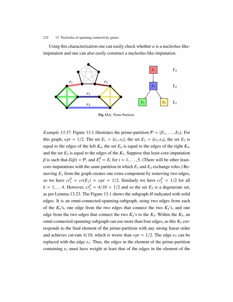
232 13 Nucleolus of spanning connectivity games
Using this characterization one can easily check whether α is a nucleolus-like-imputation and one can also easily construct a nucleolus-like-imputation.
e1 e2
e3
e4
E1
E2
E3 E4
L3
L2
L1
Fig. 13.1. Prime Partition
Example 13.37. Figure 13.1 illustrates the prime-partition P = {E1, . . . , E5}. Forthis graph, opt = 1/2. The set E1 = {e1, e2}, the set E2 = {e3, e4}, the set E3 isequal to the edges of the left K4, the set E4 is equal to the edges of the right K4,and the set E5 is equal to the edges of the K5. Suppose that least-core-imputationβ is such that E(β) = P, and Eβ
i = Ei for i = 1, . . . , 5. (There will be other least-core-imputations with the same partition in which E3 and E4 exchange roles.) Re-moving E1 from the graph creates one extra component by removing two edges,so we have crβ1 = cr(E1) = opt = 1/2. Similarly we have crβk = 1/2 for allk = 1, . . . 4. However, crβ5 = 4/10 < 1/2 and so the set E5 is a degenerate set,as per Lemma 13.23. The Figure 13.1 shows the subgraph H indicated with solidedges. It is an omni-connected-spanning-subgraph, using two edges from eachof the K4’s, one edge from the two edges that connect the two K4’s, and oneedge from the two edges that connect the two K4’s to the K5. Within the K5, anomni-connected-spanning-subgraph can use more than four edges, as this K5 cor-responds to the final element of the prime-partition with any strong linear orderand achieves cut-rate 4/10, which is worse than opt = 1/2. The edge e3 can bereplaced with the edge e1. Thus, the edges in the element of the prime-partitioncontaining e1 must have weight at least that of the edges in the element of the

13.7 Nucleolus 233
prime-partition containing e3. The right part of Figure 13.1 illustrates the partialorder O and its layers {L1, L2, L3}.
13.7 Nucleolus
We now show how to uniquely maximize the second worst excess of amongnucleolus-like-imputations. We are only interested in the case that opt < 1, sincethe graph has opt = 1 if and only if it contains a bridge. It is easy to see thatbridges are the vetoers of the SCG and the nucleolus divides payoff uniformlyamong the bridges. From here on we assume the following.
Assumption 1 opt < 1.
Before we prove how to compute the nucleolus, we need the following defini-tions.
Definition 13.38. We define L1,L2, . . . inductively as follows. The set L1 is all
the sinks of O excluding D. For j = 2, . . . , we have that L j is the set of all the
sinks when all elements of {D} ∪ (∪i=1,..., j−1Li) have been removed from O.
Note that O is defined only over nondegenerate elements of P and hence thedegenerate set is not contained in any of L1,L2, . . . .
Definition 13.39. The layers L = {L1, . . . , Lt} of G are Li = ∪E′∈Li E′ for i =
1, . . . , t.
The layers provide a way to partition the edges (except those in the degenerateset). See Figure 13.1 for an example of layers.
The following theorem shows that there is a unique least-core-imputation thatmaximizes the difference between the payoff of a worst-excess coalition and thepayoff of the second worst-excess coalition This unique least-core-imputation isthe nucleolus of the spanning connectivity game.
Theorem 13.40. Set
κ =1∑t
i=1 i · |Li|.

234 13 Nucleolus of spanning connectivity games
The nucleolus ν has ν(e) = i · κ for every i ∈ {1, . . . , t} and e ∈ Li and ν(e) = 0otherwise.
Proof. The main idea of the proof is that the weight of a connected spanningsubgraph with the second smallest weight is opt + κ, and this must be optimalsince all the weights are multiples of κ. For all other nucleolus-like-imputationsthere is second lightest connected spanning subgraph with weight less than opt+κ.
Let H be an omni-connected-spanning-subgraph and t the number of layers.Observe that
∑e∈E
ν(e) =
t∑i=1
i · |Li| · κ = κ
t∑i=1
i · |Li| = κ · κ−1 = 1
and hence ν is an edge-imputation. Note that by definition P refines E(ν) and forany e ∈ P ∈ P that is a parent of e′ ∈ P′ ∈ P we have ν(e) > ν(e′) and hence ν isa least-core-imputation and specifically a nucleolus-like-imputation.
We now show that the weight of any coalition with the second worst excess isopt + k. Afterwards we show that only ν is the only nucleolus-like-imputation forwhich the weight of any coalition with the second worst excess is at least opt + k.
Let P ∈ P be such that P ⊆ L1. Since opt < 1 Proposition 13.8 impliesthat there exists e ∈ P \ E(H). By the definition of ν we have ν(e) = κ. ByProposition 13.26 ν(H) = opt and hence ν(H ∪ {e}) = opt + κ. Note that sinceν(e′) is a multiple of κ for every e′ ∈ E there does not exist a connected spanningsubgraph H′ such that opt < ν(H′) < opt + κ.
Let α be a nucleolus-like-imputation such that the second smallest weight ofa connected spanning subgraph is at least opt + κ. We shall prove by induction on` that α(e) ≥ `κ for every e ∈ L` and every ` = 1, . . . , t. Since the only nucleolus-like-imputation that satisfies this conditions is ν this implies that α = ν.
Assume for the sake of contradiction that there exists e ∈ P ∈ L1 such thatα(e) < κ. Since opt < 1 Proposition 13.8 implies that there exists e′ ∈ P \ E(H).By Proposition 13.26 we have ν(H) = opt and hence because α(e′) = α(e) < κ
we get ν(H ∪ {e}) = opt + α(e′) < opt + κ. In addition as α is a nucleolus-like-

13.8 Wiretap game 235
imputation α(e′) > 0 and thus ν(H ∪ {e}) > opt. Yet the assumption was that forα, any coalition with the second worst excess has payoff at least opt + κ.
Assume by way of induction that for `−1 we have α(e) ≥ (`−1)κ for every e ∈
L`−1. Assume for the sake of contradiction that there exists e ∈ P ∈ L` such thatα(e) < ` · κ. By the definition of L`, there exists P′ ⊆ L`−1 such that P is a parentof P′. Consequently, there exists an omni-connected-spanning-subgraph H′, e′ ∈
P \ E(H′) and e′′ ∈ P′ ∩ E(H′) such that H∗ = (H′ \ {e′′}) ∪ {e′} is and spanningtree of G. Observe that α(H∗) = α(H′) + α(e′) − α(e′′). By Proposition 13.26,we have α(H′) = opt and hence α(H∗) = opt + α(e′) − α(e′′). By the inductionassumption, we have α(e′′) ≥ (` − 1)κ and therefore as α(e′′) = α(e) < ` · κ
we get α(H∗) < opt + κ. In addition as α is a nucleolus-like-imputation we haveα(e′) > α(e′′) and therefore ν(H∗ ∪ {e}) > opt. Yet the assumption was that for α,any coalition with the second worst excess has payoff at least opt + κ. ut
13.8 Wiretap game
Never interrupt your enemy when he is making a mistake.
- Napoleon Bonaparte
However beautiful the strategy, you should occasionally look at the re-
sults.
- Winston Churchill
In this section, we formally define the wiretap game and discusss its connec-tion to the SCG. The strategic form of the wiretap game is defined implicitly bythe graph G = (V, E). The wiretapper chooses an edge and the hider chooses aspanning subgraph of G. The wiretapper receives payoff 1 (wins), if the edge hechooses is part of the spanning subgraph chosen by the hider, and receives payoff
0 (loses) otherwise. Thus, the value of the game is the probability that the wire-tapper can secure for wiretapping the spanning subgraph chosen by the hider. Forthis reason we choose to write the game as a constant-sum, rather than zero-sumgame.

236 13 Nucleolus of spanning connectivity games
The pure strategies of the wiretapper are the edges E and the pure strategies ofthe hider are the set of spanning subgraphs S, with a typical element of S, whichis a set of edges, denoted by S .
We could define the wiretap game by only allowing the hider to pick spanningtrees. However, our defnition with connected spanning subgraphs allows a cleanconnection to the spanning connectivity game. Also, this does not change thenucleolus strategy of the wiretapper.
Let ∆(A) be the set of mixed strategies (probability distributions) on a finiteset A, and let Ia∈A be the indicator function that takes value 1 if a ∈ A and 0otherwise. By the well-known maxmin theorem for finite zero-sum games, thewiretap game Γ(G) has a unique value, defined by
val(Γ) = maxx∈∆(E)
minS∈S
∑e∈E
Ie∈S · xe = miny∈∆(S)
maxe∈E
∑S∈S
Ie∈S · yS . (13.26)
The equilibrium or maxmin strategies of the wiretapper are
{x ∈ ∆(E)|∑e∈E
Ie∈S · xe ≥ val(Γ) for all S ∈ P} . (13.27)
Playing any maxmin strategy guarantees the wiretapper to achieve a probabilityof successful wiretapping of at least val(Γ). The equilibrium or minmax strategiesof the hider are
{y ∈ ∆(P)|∑S∈P
Ie∈S · yS ≤ val(Γ) for all e ∈ E} . (13.28)
Playing any minmax strategy guarantees the hider to suffer a probability of suc-cessful wiretapping of no more than val(Γ). We have the following simple obser-vation.
Observation 13.41 The set of imputations in the least core of the SCG(G) are
the maxmin strategies of the wiretap game Γ(G).
The problem of finding a maxmin strategy of Γ(G), defined by (13.26)and (13.27), can be written as finding an x to solve

13.9 Conclusion 237
Spanning connectivity game Wiretap game
player (edge) pure strategy of wiretapperwinning coalitions pure strategies of hiderimputation wiretapper’s strategyleast-core imputation maxmin strategynucleolus-like imputation maxmin strategy minimizing no. of best responsesnucleolus unique desirable maxmin strategy1-ε1(x) min probability of successful wiretap using strategy xε1 coalition for imputation x best response to the maxmin strategy xε1 coalitions of nucleolus-like imputations best responses to every maxmin strategy
Table 13.1. Spanning connectivity game and the wiretap game
max z
s.t.∑
e∈E Ie∈S · xe ≥ z for all S ∈ S
x ∈ ∆(E)
(13.29)
It is easy to see that LP 13.1 and LP 13.29 have the same solution and objectivefunction. Therefore a least core imputation of the SCG corresponds to a maxminstrategy for the wiretapper in the wiretap game and the value of the wiretap gameis equal to the cr. Interpreted as a maxmin strategy in the wiretap game, thenucleolus of the SCG game has the following desirable properties. A nucleolus-like strategy is a maxmin strategy for the wiretapper which minimizes the numberof pure best responses of the hider. The nucleolus is the unique nucleolus-likestrategy which maximizes the gain in the probability of a successful wiretap ifthe hider fails to play a best response. We summarize the relation between theSCG and the wiretap game in Table 13.1.
13.9 Conclusion
We saw that although computing the Banzhaf values and Shapley values of theSCG are #P-complete, computing the nucleolus is in P. The idea of a principalpartition which refines the player partition for other least core payoffs may begeneralized for other cooperative games. This kind of partition can give valu-able information about the relations between the players. An interesting research

238 13 Nucleolus of spanning connectivity games
question will be to characterize, compute or utilize the principal partition forwell-known cooperative games.
Just as there is a corresponding wiretap game for a SCG, a corresponding zero-sum game can be formalized for any simple coalitional game. The maximizerplayer in the zero-sum game chooses to ‘control’ a player whereas the minimizerplayer chooses a secret winning coalition. The maximizer gets value one if hiscontrolled player is in the winning coalition chosen by the minimizer and getsvalue zero otherwise. Just like in the wiretap game, the least core is a maxminstrategy and the nucleolus is a highly desirable maxmin strategy.
There are a number of natural extensions to the wiretap game. The problemchanges if the wiretapper is allowed to pick multiple edges. If the number ofedges to be tapped is an input of the modified wiretap game, then it is interestingto investigate the complexity of the problem.

Part V
Conclusion


14
Concluding remarks
When a scientist says: “This is the very end, nobody can do anything more
here,” then he is no scientist.
- L. Gould
Not every end is the goal. The end of a melody is not its goal, and yet if a
melody has not reached its end, it has not reached its goal. A parable.
- Friedrich Nietzsche
Abstract In the thesis, open problems and conclusions for each chapter were dis-cussed individually. In the final chapter, relevant broad research issues are brieflymentioned.
In this thesis, the aim was to integrate approaches from theoretical computerscience, multiagent systems, social choice theory and cooperative game theorywith respect to simple games. Voting and resource allocation are activities notonly restricted to human societies. Virtual rational agents may also be presentin multiagent systems. Therefore, concepts from social choice theory and coop-erative game theory were shown to be highly relevant in computer science andmultiagent systems. A key conclusion of the thesis is that the algorithmic lensis fundamental in examining models and solutions in game theory. Also, com-putational complexity is an important consideration in proposing solutions anddesigning mechanisms. An algorithmic perspective in game theory promises to

242 14 Concluding remarks
play a greater role as various game theoretic concepts are used in large multiagentsystems.
The contributions of the thesis range from theoretical algorithmic and compu-tational results to practical implementations of algorithms and applied analysisof real world social choice models. The thesis also partially or fully answers anumber of open questions regarding computation of cooperative game solutionsfor simple games. In Part II, simple games were examined in detail from the per-spective of algorithmic voting theory. This included the study of computing theinfluence of players, classifying which WVGs are tractable and designing WVGs.In Part III, we contributed to a growing line of work where computational com-plexity is considered as a barrier to manipulations in voting systems. For manycases, bounds of how much manipulation can help or harm were also presentedIn Part IV, a broad survey of computational complexity of computing cooperativegame solutions for simple games was presented. Chapter 11 includes structuralresults on cooperative game solutions for monotonic cooperative game. The re-sults may shed light on computation of solutions for specific representations ofmonotonic cooperative games. In Chapters 12 and 13, we also introduced andstudied a natural cooperative game on graphs called the spanning connectivitygame.
Throughout the thesis, conclusions and open problems have been mentionedat the end of each chapter. We saw that in general, the computation of solutionsbecomes easier as we scan the following list from left to right: Shapley-Shubikindex, Banzhaf index, nucleolus, Holler index, Deegan-Packel index, least-coreand core. It is an open question to construct a representation of a simple game,where the complexity of computing the Banzhaf value is more than the complex-ity of computing the Banzhaf index. Similarly, it is an open question to construct arepresentation of a simple game, where the complexity of computing the Shapley-Shubik index is more than the complexity of computing the Banzhaf value.
In the thesis, we restricted ourselves to coalitional games with transferableutility. Coalition games with non-transferable utility have not been considered.With respect to computational complexity of manipulation, we have considered

14 Concluding remarks 243
worst case complexity. This may not be a sufficient safeguard against manipula-tion in the average case. Further research in average time complexity for manip-ulation in social choice is a recent and important direction of research.
An important assumption in the evaluation of power indices is that each coali-tion has the same probability of forming. In reality, players have ideological pref-erences or communication constraints. This may impact the actual voting powerof a player. Also, when we considered cooperative game solutions, we assumedthat the grand coalition forms and it is the value of the grand coalition which isdistributed among the players. Although, this is a natural assumption, it may notbe true in case players partition themselves.
In the thesis, we saw that computational complexity for coalitional games de-pends on the representation of the game. There is much work to be done in de-vising coalitional games which are not only expressive but also compact. Onepossible direction is to use graphs as compact ways to represent dependenciesamong players, forbidden coalitions or consistency orderings of political posi-tions. There is scope to utilize the combination of graphs and WVGs to modelcomplex decision-making scenarios. Moreover, it will be useful to develop mod-els which incorporate uncertainty of information such as values of coalitions inthe coalitional game. Some progress has already been made in that direction(see for instance [110]). On the economics front, voting power theorists are stillgrappling with the independence-of-players assumptions during the voting powercomputation. In real life, players have varying preferences in forming coalitionswith different players. It is an interesting challenge for mathematical economiststo formalize this tension in a satisfactory way.
Another area of future research is the formulation of approximate notions ofcooperative game solutions. Computer scientists have come up with approxima-tions of the Nash equilibria which may allow for easier computation. Future al-gorithmic work in coalitional games promises to follow a similar methodologywhere the trade-off between the quality of solution and computational ease is con-sidered. Within the area of coalition formation, one direction for future work isto study the computational complexity of forming stable coalitions. Although the

244 14 Concluding remarks
different stability-based cooperative game solutions predict the coalition forma-tion process, only recently have algorithmic aspects of coalition formation beenexamined. Also, most of the work in equilibria convergence considers individualplayers and not coalitions.
In most settings in cooperative game theory, it is assumed that the coalitionalgame is already known and represented. However, it may be the case that the val-ues of all coalitions are not known a priori. A relevant research problem is that oflearning a coalitional game while minimizing the number of queries. In general,a coalitional game requires a query per coalition. However, when the coalitionalgame contains some structure (like monotonicity) or belongs to a particular classof coalitional games, there is a need to devise efficient algorithms to efficientlyconstruct the game exactly or approximately. The research will involve using thelatest tools from learning theory and applying them to cooperative game theory.
Part IV of the thesis examined problems of resource allocation on networks.We considered settings where the value of each coalition is already known andpublic. In many cases such as auctions, players and coalitions have private val-ues. In resource allocation, there is a growing line of research on how to designresource allocation where players have incentive to provide truthful valuations.There is huge scope for further research on combinatorial optimization gamesand cost sharing on networks. This will better inform us how to incentivize co-operation in peer-to-peer settings and also how to share and price resources onnetworks. This economics-driven approach is likely to make an impact in futureengineering and design issues in networks.

Part VI
Appendices

A
MWVG Program
(Based on Chapter 5)
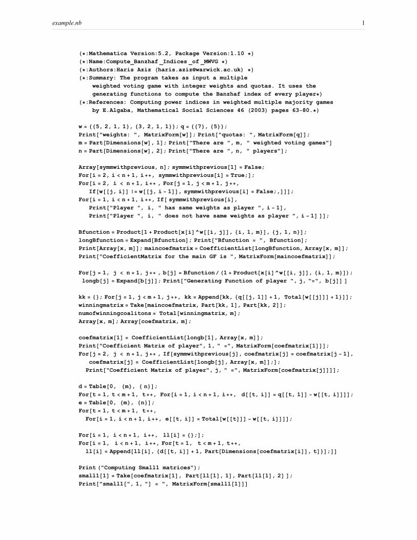
H∗:Mathematica Version:5.2, Package Version:1.10 ∗L
H∗:Name:Compute_Banzhaf _Indices _of _MWVG ∗L
H∗:Authors:Haris Aziz [email protected] ∗L
H∗:Summary: The program takes as input a multiple
weighted voting game with integer weights and quotas. It uses the
generating functions to compute the Banzhaf index of every player∗L
H∗:References: Computing power indices in weighted multiple majority games
by E.Algaba, Mathematical Social Sciences 46 H2003L pages 63−80.∗L
w = 885, 2, 1, 1<, 83, 2, 1, 1<<; q = 887<, 85<<;
Print@"weights: ", MatrixForm@wDD; Print@"quotas: ", MatrixForm@qDD;
m = Part@Dimensions@wD, 1D; Print@"There are ", m, " weighted voting games"D
n = Part@Dimensions@wD, 2D; Print@"There are ", n, " players"D;
Array@symmwithprevious, nD; symmwithprevious@1D = False;
For@i = 2, i < n + 1, i++, symmwithprevious@iD = True;D;
For@i = 2, i < n + 1, i++ , For@j = 1, j < m + 1, j++,
If@w@@j, iDD != w@@j, i − 1DD, symmwithprevious@iD = False;,DDD;
For@i = 1, i < n + 1, i++, If@ symmwithprevious@iD,
Print@"Player ", i, " has same weights as player ", i − 1D,
Print@"Player ", i, " does not have same weights as player ", i − 1D DD;
Bfunction = Product@1 + Product@x@iD^w@@i, jDD, 8i, 1, m<D, 8j, 1, n<D;
longBfunction = Expand@BfunctionD; Print@"Bfunction = ", BfunctionD;
Print@Array@x, mDD; maincoefmatrix = CoefficientList@longBfunction, Array@x, mDD;
Print@"CoefficientMatrix for the main GF is ", MatrixForm@maincoefmatrixDD;
For@j = 1, j < n + 1, j++ , b@jD = BfunctionêH1 + Product@x@iD^w@@i, jDD, 8i, 1, m<DL;
longb@jD = Expand@b@jDD; Print@"Generating Function of player ", j, "=", b@jDD D
kk = 8<; For@j = 1, j < m + 1, j++, kk = Append@kk, 8q@@j, 1DD + 1, Total@w@@jDDD + 1<DD;
winningmatrix = Take@maincoefmatrix, Part@kk, 1D, Part@kk, 2DD;
numofwinningcoalitons = Total@winningmatrix, mD;
Array@x, mD; Array@coefmatrix, mD;
coefmatrix@1D = CoefficientList@longb@1D, Array@x, mDD;
Print@"Coefficient Matrix of player", 1, " =", MatrixForm@coefmatrix@1DDD;
For@j = 2, j < n + 1, j++ , If@symmwithprevious@jD, coefmatrix@jD = coefmatrix@j − 1D,
coefmatrix@jD = CoefficientList@longb@jD, Array@x, mDD;D;
Print@"Coefficient Matrix of player", j, " =", MatrixForm@coefmatrix@jDDDD;
d = Table@0, 8m<, 8 n<D;
For@t = 1, t < m + 1, t++, For@i = 1, i < n + 1, i++, d@@t, iDD = q@@t, 1DD − w@@t, iDDDD;
e = Table@0, 8m<, 8n<D;
For@t = 1, t < m + 1, t++,
For@i = 1, i < n + 1, i++, e@@t, iDD = Total@w@@tDDD − w@@t, iDDDD;
For@i = 1, i < n + 1, i++, ll@iD = 8<;D;
For@i = 1, i < n + 1, i++, For@t = 1, t < m + 1, t++,
ll@iD = Append@ll@iD, 8d@@t, iDD + 1, Part@Dimensions@coefmatrix@iDD, tD<D;DD
Print H"Computing Small1 matrices"L;
small1@1D = Take@coefmatrix@1D, Part@ll@1D, 1D, Part@ll@1D, 2D D;
Print@"small1@", 1, "D = ", MatrixForm@small1@1DDD
example.nb 1

For@i = 2, i < n + 1, i++, If@symmwithprevious@iD, small1@iD = small1@i − 1D,
small1@iD = Take@coefmatrix@iD, Part@ll@iD, 1D, Part@ll@iD, 2D DD;
Print@"small1@", i, "D = ", MatrixForm@small1@iDDDD;
For@i = 1, i < n + 1, i++, sum1@iD = Total@small1@iD, InfinityD;
Print@"sum1@", i, "D = ", sum1@iDDD;
g = Table@0, 8m<, 8n<D;
For@t = 1, t < m + 1, t++,
For@i = 1, i < n + 1, i++, g@@t, iDD = Total@w@@tDDD − w@@t, iDD + 1;DD;
mm@1D = 8<; For@i = 1, i < n + 1, i++, mm@iD = 8<;D ;
Array@errorcheck, nD;
For@z = 1, z < n + 1, z++, errorcheck@zD = 0;D;
For@i = 1, i < n + 1, i++,
For@t = 1, t < m + 1, t++, mm@iD = Append@mm@iD, 8q@@t, 1DD + 1, g@@t, iDD<D;
If@q@@t, 1DD + 1 > g@@t, iDD, errorcheck@iD = 1;,D;D D;
For@i = 1, i < n + 1, i++, If@errorcheck@iD == 1, small2@iD = 8<,
small2@iD = Take@coefmatrix@iD, Part@mm@iD, 1D, Part@mm@iD, 2D DD;
Print@"small2@", i, "D = ", MatrixForm@small2@iDDDD;
For@i = 1, i < n + 1, i++, If@small2@iD == 8<, sum2@iD = 0,
sum2@iD = Total@small2@iD, InfinityDD; Print@"sum2@", i, "D = ", sum2@iDDD;
totalswings = 0;
For@i = 1, i < n + 1, i++, swings@iD = sum1@iD − sum2@iD;
totalswings = totalswings + swings@iD; Print@"swings@", i, "D = ", swings@iDDD;
For@i = 1, i < n + 1, i++, banzhafindex@iD = swings@iDêtotalswings;
Print@"Banzhaf Index of player", i, " is ", banzhafindex@iDDD;
vetoplayerlist = 8<;
For@i = 1, i < n + 1, i++, isvetoplayer = False; For@j = 1, j < m + 1, j++,
If@HTotal@w@@jDDD − w@@j, iDDL < q@@j, 1DD, isvetoplayer = True;, D D;
If@isvetoplayer, vetoplayerlist = Append@vetoplayerlist, iD;
Print@i, " has veto powers"D, Print@i, " does not have veto powers"DDD
Print@"Number of winning coalitions = ", numofwinningcoalitonsD;
weights: J 5 2 1 1
3 2 1 1N
quotas: J 75N
There are 2 weighted voting games
There are 4 players
Player 1 does not have same weights as player 0
Player 2 does not have same weights as player 1
Player 3 does not have same weights as player 2
Player 4 has same weights as player 3
Bfunction = H1 + x@1D x@2DL2 H1 + x@1D2 x@2D2L H1 + x@1D5 x@2D3L
8x@1D, x@2D<
example.nb 2

CoefficientMatrix for the main GF is
i
k
jjjjjjjjjjjjjjjjjjjjjjjjjjjjjjjjjjjjjjjj
1 0 0 0 0 0 0 0
0 2 0 0 0 0 0 0
0 0 2 0 0 0 0 0
0 0 0 2 0 0 0 0
0 0 0 0 1 0 0 0
0 0 0 1 0 0 0 0
0 0 0 0 2 0 0 0
0 0 0 0 0 2 0 0
0 0 0 0 0 0 2 0
0 0 0 0 0 0 0 1
y
{
zzzzzzzzzzzzzzzzzzzzzzzzzzzzzzzzzzzzzzzz
Generating Function of player 1=H1 + x@1D x@2DL2 H1 + x@1D2 x@2D2L
Generating Function of player 2=H1 + x@1D x@2DL2 H1 + x@1D5 x@2D3L
Generating Function of player 3=H1 + x@1D x@2DL H1 + x@1D2 x@2D2L H1 + x@1D5 x@2D3L
Generating Function of player 4=H1 + x@1D x@2DL H1 + x@1D2 x@2D2L H1 + x@1D5 x@2D3L
Coefficient Matrix of player1 =
i
k
jjjjjjjjjjjjjjjj
1 0 0 0 0
0 2 0 0 0
0 0 2 0 0
0 0 0 2 0
0 0 0 0 1
y
{
zzzzzzzzzzzzzzzz
Coefficient Matrix of player2 =
i
k
jjjjjjjjjjjjjjjjjjjjjjjjjjjjjj
1 0 0 0 0 0
0 2 0 0 0 0
0 0 1 0 0 0
0 0 0 0 0 0
0 0 0 0 0 0
0 0 0 1 0 0
0 0 0 0 2 0
0 0 0 0 0 1
y
{
zzzzzzzzzzzzzzzzzzzzzzzzzzzzzz
Coefficient Matrix of player3 =
i
k
jjjjjjjjjjjjjjjjjjjjjjjjjjjjjjjjjjj
1 0 0 0 0 0 0
0 1 0 0 0 0 0
0 0 1 0 0 0 0
0 0 0 1 0 0 0
0 0 0 0 0 0 0
0 0 0 1 0 0 0
0 0 0 0 1 0 0
0 0 0 0 0 1 0
0 0 0 0 0 0 1
y
{
zzzzzzzzzzzzzzzzzzzzzzzzzzzzzzzzzzz
Coefficient Matrix of player4 =
i
k
jjjjjjjjjjjjjjjjjjjjjjjjjjjjjjjjjjj
1 0 0 0 0 0 0
0 1 0 0 0 0 0
0 0 1 0 0 0 0
0 0 0 1 0 0 0
0 0 0 0 0 0 0
0 0 0 1 0 0 0
0 0 0 0 1 0 0
0 0 0 0 0 1 0
0 0 0 0 0 0 1
y
{
zzzzzzzzzzzzzzzzzzzzzzzzzzzzzzzzzzz
small1@1D =
i
k
jjjjjj2 0 0
0 2 0
0 0 1
y
{
zzzzzz
small1@2D =
i
k
jjjjjj1 0 0
0 2 0
0 0 1
y
{
zzzzzz
small1@3D =
i
k
jjjjjj1 0 0
0 1 0
0 0 1
y
{
zzzzzz
small1@4D =
i
k
jjjjjj1 0 0
0 1 0
0 0 1
y
{
zzzzzz
example.nb 3
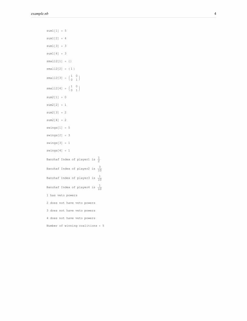
sum1@1D = 5
sum1@2D = 4
sum1@3D = 3
sum1@4D = 3
small2@1D = 8<
small2@2D = H 1 L
small2@3D = J 1 0
0 1N
small2@4D = J 1 0
0 1N
sum2@1D = 0
sum2@2D = 1
sum2@3D = 2
sum2@4D = 2
swings@1D = 5
swings@2D = 3
swings@3D = 1
swings@4D = 1
Banzhaf Index of player1 is1����2
Banzhaf Index of player2 is3�������10
Banzhaf Index of player3 is1�������10
Banzhaf Index of player4 is1�������10
1 has veto powers
2 does not have veto powers
3 does not have veto powers
4 does not have veto powers
Number of winning coalitions = 5
example.nb 4


Part VII
Backmatter

References
1. E. Algaba, J. M. Bilbao, and J. R. Fernandez, The distribution of power in the European Constitution,
European Journal of Operational Research 176 (2007), no. 3, 1752–1755. [16, 78, 108]
2. E. Algaba, J. M. Bilbao, J. R. Fernandez Garcia, and J. J. Lopez, Computing power indices in weighted
multiple majority games, Mathematical Social Sciences 46 (2003), no. 1, 63–80. [24, 73]
3. N. Alon and P. Edelman, The inverse Banzhaf problem, Social Choice and Welfare 10.1007/s00355-009-0402-8 (2009). [84]
4. J.M Alonso-Meijide, Generating functions for coalition power indices: An application to the IMF,
Annals of Operations Research 137 (2005), 21–44. [78]
5. G. Arcaini and G. Gambarelli, Algorithm for automatic computation of the power variations in share
tradings, Calcolo 23 (1986), no. 1, 13–19. [78, 108]
6. S. Arnborg, D. G. Corneil, and A. Proskurowski, Complexity of finding embeddings in a k-tree, SIAM
J. Algebraic Discrete Methods 8 (1987), no. 2, 277–284. [194]
7. S. Arnborg and A. Proskurowski, Linear time algorithms for NP-hard problems restricted to partial
k-trees, Discrete Appl. Math. 23 (1989), no. 1, 11–24. [194]
8. K. J. Arrow, Social choice and individual values (2nd edition), Wiley, New York, 1963. [69]
9. R. J. Aumann, B. Peleg, and P. Rabinowitz, A method for computing the kernel of n-person games,
Mathematics of Computation 19 (1965), no. 92, 531–551. [165, 177]
10. H. Aziz, Complexity of comparison of influence of players in simple games, Proceedings of the Second
International Workshop on Computational Social Choice (COMSOC 2008), 2008, pp. 61–72. [XVII,
17]
11. , Simple games: complexity of length, duality and bribery, European Workshop on Multiagent
Systems (2008). [XVII, 20]
12. H. Aziz, F. Brandt, and P. Harrenstein, Monotone cooperative games and their threshold versions,
Submitted (2009). [171]
13. H. Aziz, O. Lachish, M. Paterson, and R. Savani, Power indices of spanning connectivity games, The
5th International Conference on Algorithmic Aspects in Information and Management (AAIM), 2009.
[XVII, 21]
14. , Wiretapping a hidden network, Tech. report, http://arxiv.org/abs/0909.5293, 2009. [XVII, 21]

256 References
15. H. Aziz and M. Paterson, Computational and combinatorial aspects of multiple weighted voting
games, Algorithms and Complexity in Durham - Proceedings of the Third ACiD Workshop, Texts
in Algorithmics, King’s College, London, 2007. [XVII, 18]
16. , Classification of computationally tractable weighted voting games, Lecture Notes in Engi-
neering and Computer Science, World Congress on Engineering 1 (2008), 129–134. [XVII, 18, 67,
132]
17. , Complexity of some aspects of control and manipulation in weighted voting games, Annales
du Lamsade, Proceedings of the DIMACS-LAMSADE Workshop on Algorithmic Decision Theory
2008, 2008. [XVII, 19]
18. , False name manipulations in weighted voting games: splitting, merging and annexation, AA-
MAS ’09: Proceedings of The 8th International Conference on Autonomous Agents and Multiagent
Systems, 2009, pp. 409–416. [XVII, 20]
19. H. Aziz, M. Paterson, and D. Leech, Efficient algorithm for designing weighted voting games, Multi-
topic Conference, 2007. INMIC 2007. IEEE International (2007), 1–6. [XVII, 19]
20. R. Bacher, Determinants of matrices related to the pascal triangle, J. Theor. des Nombres Bordeaux
14 (2002), 19–41. [49, 191]
21. Y. Bachrach and E. Elkind, Divide and conquer: False-name manipulations in weighted voting games,
The Seventh International Joint Conference on Autonomous Agents and Multiagent Systems (AAMAS
2008) (Estoril, Portual), May 2008, pp. 975–982. [108, 116, 117, 118, 122, 124, 131, 132]
22. Y. Bachrach, E. Markakis, A. D. Procaccia, J. S. Rosenschein, and A. Saberi, Approximating power
indices, AAMAS, 2008, pp. 943–950. [66, 197, 198]
23. Y. Bachrach, R. Meir, M. Zuckerman, J. Rothe, and J. S. Rosenschein, The cost of stability in weighted
voting games (extended abstract), The Eighth International Joint Conference on Autonomous Agents
and Multiagent Systems (AAMAS 2009) (Budapest, Hungary), May 2009. [181, 184]
24. Y. Bachrach and J. S. Rosenschein, Computing the Banzhaf power index in network flow games, AA-
MAS ’07: Proceedings of the 6th International Joint conference on Autonomous agents and multiagent
systems (New York, NY, USA), ACM, 2007, pp. 1–7. [187]
25. Y. Bachrach and J. S. Rosenschein, Coalitional skill games, AAMAS, 2008, pp. 1023–1030. [51]
26. , Power in threshold network flow games, Journal of Autonomous Agents and Multi-Agent
Systems 18 (2009), no. 1, 106–132. [51, 156]
27. Y. Bachrach, J. S. Rosenschein, and E. Porat, Power and stability in connectivity games, AAMAS,
2008, pp. 999–1006. [51, 187]
28. R. A. Bailey, Surveys in combinatorics, Cambridge University Press, 1997. [190]
29. M. O. Ball, Computational complexity of network reliability analysis: An overview, IEEE Transactions
on Reliability 35 (1986), no. 3, 230–239. [187, 189, 190]
30. M. O. Ball and J. S. Provan, Disjoint products and efficient computation of reliability, Oper. Res. 36(1988), no. 5, 703–715. [47]
31. J. F. Banzhaf, Weighted voting doesn’t work, Rutgers Law Review 19 (1965), 317–343. [25]
32. J. Bartholdi, III and J. Orlin, Single transferable vote resists strategic voting., Social Choice and Wel-
fare 8 (1991), no. 4, 341–354. [124]
33. D. Bean, J. Friedman, and C. Parker, Simple majority achievable hierarchies, Theory and Decision 65(2008), no. 4, 285–302. [79]

References 257
34. B. Ben-Moshe and Y. Dinitz, Fast additive constant approximation algorithms for the safe deposit
boxes problem with two and three currencies, Proceedings of the 19th Annual Canadian Conference
on Computational Geometry, CCCG, 2007, pp. 53–56. [140]
35. T. Bietenhader and Y. Okamoto, Core stability of minimum coloring games, Math. Oper. Res. 31(2006), no. 2, 418–431. [166]
36. J. M. Bilbao, J. R. Fernandez, A. Jimenez Losada, and J. J. Lopez, Generating functions for computing
power indices efficiently, citeseer.ist.psu.edu/452269.html (2000). [64, 65, 67, 81, 124]
37. J. C. Bioch and T. Ibaraki, Complexity of identification and dualization of positive boolean functions,
Inf. Comput. 123 (1995), no. 1, 50–63. [144]
38. P. Borm, H. Hamers, and R. Hendrickx, Operations research games: A survey, TOP: An Official Jour-
nal of the Spanish Society of Statistics and Operations Research 9 (2001), no. 2, 139–199. [155, 187]
39. S. F. Brams and P. J. Affuso, Power and size: A new paradox, Theory and Decision 7 (1976), 29–56.
[65, 67]
40. U. Brandes and T. Erlebach, Network analysis: Methodological foundations, Springer, 2005. [198]
41. F. Carreras, On the design of voting games, Mathematical Methods of Operations Research 59 (2004),
no. 1, 503–515. [80]
42. F. Carreras and J. Freixas, Complete simple games, Mathematical Social Sciences 32 (1996), no. 2,
139–155. [36]
43. N. Chakravarty, A. M. Goel, and T. Sastry, Easy weighted majority games, Mathematical Social Sci-
ences 40 (2000), no. 2, 227–235. [61, 63, 64, 67]
44. V. Chandru and M. R. Rao, Linear programming, Algorithms and Theory of Computation Handbook,
CRC Press, 1999. [141]
45. E. Cheng and W. H. Cunningham, A faster algorithm for computing the strength of a network, Inf.
Process. Lett. 49 (1994), no. 4, 209–212. [219]
46. Y. Chevaleyre, P. E. Dunne, U. Endriss, J. Lang, M. Lemaitre, N. Maudet, J. Padget, S. Phelps, J. A.
Rodrıguez-Aguilar, and P. Sousa, Issues in multiagent resource allocation, Informatica 30 (2006),
no. 1, 3–31. [155]
47. Y. Chevaleyre, U. Endriss, J. Lang, and N. Maudet, A short introduction to computational social
choice, Proceedings of the 33rd Conference on Current Trends in Theory and Practice of Computer
Science (SOFSEM-2007), LNCS, vol. 4362, Springer-Verlag, January 2007, pp. 51–69. [10]
48. C. K. Chow, On the characterization of threshold functions, FOCS, 1961, pp. 34–38. [27]
49. J. S. Coleman, Control of collectivities and the power of a collectivity to act, Social Choice (B. Lieber-
man, ed.), New York, 1971, pp. 269–300. [26]
50. V. Conitzer and T. Sandholm, Complexity of manipulating elections with few candidates, Eighteenth
National Conference on Artificial Intelligence (Menlo Park, CA, USA), American Association for
Artificial Intelligence, 2002, pp. 314–319. [145]
51. P. G. D. Cortona, C. Manzi, A. Pennisi, F. Ricca, and B. Simeone, Evaluation and optimization of
electoral systems (Monographs on Discrete Mathematics and Applications), Society for Industrial
Mathematics, 1987. [145]
52. Y. Crama and L. Leruth, Control and voting power in corporate networks: Concepts and computational
aspects, European Journal of Operational Research 178 (2007), no. 3, 879–893. [187]
258 References
53. W. H. Cunningham, Optimal attack and reinforcement of a network, J. ACM 32 (1985), no. 3, 549–561.
[201, 205, 219]
54. I. Curiel, Cooperative game theory and applications: Cooperative games arising from combinatorial
optimization problems, Springer, 1997. [155, 187]
55. B. B. de Mesquita, Minimum winning coalition, in politics, Neil J. Smelser and Paul B. Baltes,
Editor(s)-in-Chief, International Encyclopedia of the Social & Behavioral Sciences (2001), 9889–
9891. [27]
56. J. Deegan and E. W. Packel, A new index of power for simple n-person games, International Journal of
Game Theory 7 (1978), no. 2, 113–123. [27]
57. V. G. Deineko and G. J. Woeginger, On the dimension of simple monotonic games, European Journal
of Operational Research 170 (2006), no. 1, 315–318. [36, 37, 71]
58. X. Deng and Q. Fang, Algorithmic cooperative game theory, Pareto Optimality, Game Theory And
Equilibria, Springer Optimization and Its Applications, vol. 17, Springer, 2008, pp. 159–185. [13, 155,
172, 183]
59. X. Deng, Q. Fang, and X. Sun, Finding nucleolus of flow game, SODA ’06: Proceedings of the Seven-
teenth Annual ACM-SIAM Symposium on Discrete Algorithms (New York, NY, USA), ACM, 2006,
pp. 124–131. [174, 201]
60. X. Deng and C. H. Papadimitriou, On the complexity of cooperative solution concepts, Math. Oper.
Res. 19 (1994), no. 2, 257–266. [46, 155, 184]
61. E. A. Dinic and A. V. Karzanov, Boolean optimization problems with uniform constraints, Institute for
Control Sci. (1978), Reprint. [139]
62. T. Driessen, Cooperative games, solutions and applications, Kluwer Academic Publishers, Dordrecht,
The Netherlands, 1988. [155, 160]
63. P. Dubey and L. S. Shapley, Mathematical properties of the Banzhaf power index, Mathematics of
Operations Research 4 (1979), no. 2, 99–131. [27, 118, 143]
64. E. Einy, The desirability relation of simple games, Mathematical Social Sciences 10 (1985), no. 2,
155–168. [36]
65. E. Einy and D. Wettstein, Equivalence between bargaining sets and the core in simple games, Interna-
tional Journal of Game Theory 25 (1996), no. 1, 65–71. [162, 179]
66. T. Eiter, K. Makino, and G. Gottlob, Computational aspects of monotone dualization: A brief survey,
Discrete Applied Mathematics 156 (2008), no. 11, 2035–2049. [144]
67. E. Elkind, Private communication, 2009. [120]
68. E. Elkind, L. A. Goldberg, P. Goldberg, and M. Wooldridge, Computational complexity of weighted
threshold games, AAAI-07 (Twenty-Second National Conference on Artificial Intelligence) (2007),
718–723. [155, 158, 163, 164, 165, 167, 173, 175, 180, 182, 184, 201]
69. , On the dimensionality of voting games, Proceedings of the Twenty-Third AAAI Conference
on Artificial Intelligence (AAAI-2008) (Chicago, Illinois, USA), July 13-17 2008. [37, 108]
70. E. Elkind and D. Pasechnik, Computing the nucleolus of weighted voting games, SODA ’09: Proceed-
ings of the Nineteenth Annual ACM -SIAM Symposium on Discrete Algorithms (Philadelphia, PA,
USA), 2009, pp. 327–335. [155, 174, 180, 201]
71. K. Engel, Sperner theory, Cambridge University Press, New York, NY, USA, 1997. [16]
References 259
72. A. Fabrikant, C. H Papadimitriou, and K. Talwar, The complexity of pure Nash equilibria, STOC ’04:
Proceedings of the Thirty-Sixth Annual ACM Symposium on Theory of Computing (New York, NY,
USA), ACM, 2004, pp. 604–612. [11]
73. U. Faigle, W. Kern, and J. Kuipers, Computing the nucleolus of min-cost spanning tree games is NP-
hard, Int. J. Game Theory 27 (1998), no. 3, 443–450. [174, 201]
74. , Computing an element in the lexicographic kernel of a game, Mathematical Methods of Op-
erations Research 63 (2006), no. 3, 427–433. [178]
75. P. Faliszewski, E. Hemaspaandra, L. Hemaspaandra, and J. Rothe, A richer understanding of the com-
plexity of election systems, Fundamental Problems in Computing: Essays in Honor of Professor Daniel
J. Rosenkrantz (S. Ravi and S. Shukla, eds.), 2009. [145]
76. P. Faliszewski and L. A. Hemaspaandra, The complexity of power-index comparison, AAIM, 2008,
pp. 177–187. [46]
77. Piotr Faliszewski, Edith Elkind, and Michael Wooldridge, Boolean combinations of weighted voting
games, AAMAS ’09: Proceedings of The 8th International Conference on Autonomous Agents and
Multiagent Systems, 2009, pp. 185–192. [69]
78. Q. Fang, Nucleolus, Encyclopedia of Algorithms, 2008. [173]
79. Q. Fang and L. Kong, Core stability of vertex cover games, WINE, 2007, pp. 482–490. [166]
80. S. S. Fatima, M. Wooldridge, and N. R. Jennings, A randomized method for the Shapley value for
the voting game, AAMAS ’07: Proceedings of the 6th International Joint Conference on Autonomous
Agents and Multiagent Systems (New York, NY, USA), ACM, 2007, pp. 1–8. [66]
81. J. Feigenbaum, D. C. Parkes, and D. M. Pennock, Computational challenges in e-commerce, Commun.
ACM 52 (2009), no. 1, 70–74. [10]
82. D. Felsenthal and M. Machover, The measurement of voting power, Edward Elgar Publishing, Chel-
tenham, UK, 1998. [53, 82, 117, 126, 130, 131]
83. D. S. Felsenthal and M. Machover, Analysis of QM rules in the draft constitution for Europe proposed
by the European Convention, 2003, Social Choice and Welfare 23 (2004), no. 1, 1–20. [78]
84. D. S. Felsenthal and M. Machover, Analysis of QM rule adopted by the council of the european union,
23 june 2007, Tech. report, 2007. [94]
85. R. Fidytek, A. W. Mostowski, R. Somla, and A. Szepietowski, Algorithms counting monotone boolean
functions, Inf. Process. Lett. 79 (2001), no. 5, 203–209. [16]
86. M. L. Fredman and L. Khachiyan, On the complexity of dualization of monotone disjunctive normal
forms, J. Algorithms 21 (1996), no. 3, 618–628. [144]
87. J. Freixas, Bounds for Owen’s multilinear extension, J. Appl. Probab. 44 (2007)), no. 4, 852–864. [66]
88. J. Freixas, X. Molinero, M. Olsen, and M. J. Serna, The complexity of testing properties of simple
games, CoRR abs/0803.0404 (2008). [34, 37]
89. J. Freixas and M. A. Puente, Amplitude of weighted majority systems: strict representations, Questiio
23 (1999), no. 1, 43–60. [109, 110]
90. , A note about games-composition dimension, Discrete Appl. Math. 113 (2001), no. 2-3, 265–
273. [71]
91. J. Freixas and M. A. Puente, Dimension of complete simple games with minimum, European Journal
of Operational Research 127 (2008), no. 2, 555–568. [37]
260 References
92. A. Freville, The multidimensional 0-1 knapsack problem: An overview, European Journal of Opera-
tional Research 127 (2004), no. 1, 1–21. [138]
93. S. Fujishige, Submodular functions and optimization, Annals of Discrete Mathematics, vol. 58, Else-
vier, 2005. [201]
94. G. Gambarelli, Power indices for political and financial decision making: A review, Annals of Opera-
tions Research 51 (1994), 1572–9338. [15, 78, 108]
95. M. R. Garey and D. S. Johnson, Computers and intractability, a guide to the theory of NP-
completeness, Freeman, 1979. [111]
96. G. Gens and E. Levner, Complexity of approximation algorithms for combinatorial problems: a survey,
SIGACT News 12 (1980), no. 3, 52–65. [139, 141]
97. A. Gibbard, Manipulation of voting schemes: A general result, Econometrica 41 (1973), no. 4, 587–
601. [108]
98. D. B. Gillies, Solutions to general non-zero-sum games, Contributions to the Theory of Games IV
(A. W. Tucker and R. D. Luce, eds.), (Annals of Mathematics Studies), vol. 40, Princeton University
Press, 1959, pp. 47–85. [159]
99. C. Godsil and G. Royle, Algebraic graph theory, Springer, April 2001. [197]
100. P. W. Goldberg, A bound on the precision required to estimate a boolean perceptron from its average
satisfying assignment, SIAM J. Discret. Math. 20 (2006), no. 2, 328–343. [48]
101. D. Granot and M. Maschler, Spanning network games, International Journal of Game Theory 27(1998), no. 4, 467–500. [187]
102. D. Granot, M. Maschler, G. Owen, and W. R. Zhu, The kernel/nucleolus of a standard tree game,
International Journal of Game Theory 25 (1996), no. 2, 219–44. [174, 201]
103. D. Gusfield, Connectivity and edge-disjoint spanning trees, Inf. Process. Lett. 16 (1983), no. 2, 87–89.
[200, 205]
104. E. Hemaspaandra and L. A. Hemaspaandra, Dichotomy for voting systems, J. Comput. Syst. Sci. 73(2007), no. 1, 73–83. [145]
105. M. Hilliard, Weighted voting theory and applications, Tech. Report No. 609, School of Operations
Research and Industrial Engineering, Cornell University, 1983. [42]
106. M. J. Holler, Forming coalitions and measuring voting power, Political Studies 30 (1982), no. 2, 262–
271. [27]
107. R. Holzman, E. Lehrer, and N. Linial, Some bounds for the Banzhaf index and other semivalues, Math.
Oper. Res. 13 (1988), no. 2, 358–363. [66]
108. E. Horowitz and S. Sahni, Computing partitions with applications to the knapsack problem, J. ACM
21 (1974), no. 2, 277–292. [54, 73]
109. S-T. Hu, Threshold logic, University of California Press, Berkeley and Los Angeles, 1965. [16, 37, 109,
110]
110. S. Ieong and Y. Shoham, Bayesian coalitional games, AAAI, 2008, pp. 95–100. [243]
111. J. Bartholdi III, C. Tovey, and M. Trick., The computational difficulty of manipulating an election.,
Social Choice and Welfare 6 (1989), no. 3, 227–241. [124]
112. , Voting schemes for which it can be difficult to tell who won the election., Social Choice and
Welfare 6 (1989), no. 2, 157–165. [124]

References 261
113. A. Iwasaki, D. Kempe, Y. Saito, M. Salek, and M. Yokoo, False-name-proof mechanisms for hiring a
team, WINE, 2007, pp. 245–256. [117]
114. III J. Bartholdi, C. Tovey, and M. Trick., How hard is it to control an election?, Mathematical and
Computer Modeling 16 (1992), no. 8/9, 27–40. [115, 124]
115. D. Johnson, Challenges for theoretical computer science, http://www.research.att.com/∼dsj/nsflist.html
(2000). [15]
116. G. Kalai and S. Safra, Threshold phenomena and influence: perspectives from mathematics, computer
science, and economics, Computational complexity and statistical physics, St. Fe Inst. Stud. Sci. Com-
plex., Oxford Univ. Press, New York, 2006, pp. 25–60. MR MR2208732 [14, 33]
117. R. M. Karp, Combinatorics, complexity, and randomness, Commun. ACM 29 (1986), no. 2, 98–109.
[9]
118. W. Kern and D. Paulusma, Matching games: The least core and the nucleolus, Math. Oper. Res. 28(2003), no. 2, 294–308. [182]
119. J. Kleinberg, The convergence of social and technological networks, Commun. ACM 51 (2008), no. 11,
66–72. [11]
120. D. Kleitman, On Dedekind’s problem: The number of monotone boolean functions, Proceedings of the
American Mathematical Society 21 (1969), no. 3, 677–682. [15]
121. B. Klinz and G. J. Woeginger, Faster algorithms for computing power indices in weighted voting
games, Mathematical Social Sciences 49 (2005), no. 1, 111–116. [54, 67, 73]
122. A. Kopelowitz, Computation of the kernels of simple games and the nucleolus of n-person games,
Math. Dept., The Hebrew University of Jerusalem (1967), no. RM-31. [174]
123. B. Korte and J. Vygen, Combinatorial optimization: Theory and algorithms, 3rd ed., Springer, Ger-
many, 2006. [50, 191]
124. I. Krohn and P. Sudholter, Directed and weighted majority games, Mathematical Methods of Opera-
tions Research 42 (1995), no. 2, 189–216. [180]
125. J. Kuipers, A polynomial algorithm for computing the nucleolus of convex games., Tech. rep., Univ. of
Maastricht M 96-12 (1996). [174, 201]
126. K. Jeroen Kuipers, U. Faigle, and W. Kern, On the computation of the nucleolus of a cooperative game,
International Journal of Game Theory 30 (2001), no. 1, 79–98. [174, 201]
127. D. M. Kilgour L. Fang, K. W. Hipel, Interactive decision making: The graph model for conflict reso-
lution (wiley series in systems engineering and management), John Wiley & Sons, New York, 1993.
[12]
128. Lamsade and Dimacs, Dimacs-Lamsade partnership, 2008, http://www.lamsade.dauphine.fr/dimacs/.
[14]
129. J-E Lane and R. Maeland, Constitutional analysis: The power index approach, European Journal of
Political Research 37 (2000), 31–56. [78]
130. A. Laruelle and M. Widgren, Is the allocation of voting power among EU states fair?, Public Choice
94 (1998), no. 3-4, 317–39. [78, 79, 108]
131. D. Leech, Computation of power indices, Warwick Economic Resarch Papers (2002), no. 644. [66]
132. , An empirical comparison of the performance of classical power indices, Political Studies 50(2002), no. 1, 1–22. [53]

262 References
133. , Designing the Voting System for the Council of the European Union, Public Choice 113(2002), no. 3-4, 437–64. [89]
134. , Voting Power in the Governance of the International Monetary Fund, Annals of Operations
Research 109 (2002), no. 1, 375–397. [78, 108]
135. , Computing power indices for large voting games, Management Science 49 (2003), no. 6,
831–837. [66, 80]
136. , Power indices as an aid to institutional design: the generalised apportionment problem, Year-
book on New Political Economy, edited by M. Holler, H.Kliemt, D. Schmidtchen and M. Streit. (2003).
[79]
137. D. Leech and H. Aziz, The double majority voting rule of the EU reform treaty as a democratic ideal
for an enlarging union: an appraisal using voting power analysis, W. Slomczynski and K. Zyczkowski
eds., Distribution of Power and voting procedures in the European Union, Ashgate, 2009. [XVII, 19]
138. N. Linial, Game-theoretic aspects of computing, Handbook of Game Theory with Economic Applica-
tions (R. J. Aumann and S. Hart, eds.). [10]
139. F. W. Lucas, Von Neumann-Morgenstern Stable Sets, Handbook of Game Theory 1 (1962), 543–590.
[160]
140. , The proof that a game may not have a solution, Transactions of the American Mathematical
Society 136 (1969), no. 2, 219–229. [160]
141. W. F. Lucas, Von neumann-morgenstern stable sets, Handbook of Game Theory with Economic Ap-
plications (R. J. Aumann and S. Hart, eds.). [159]
142. Maschler M., B. Peleg, and L. S. Shapley, Geometric properties of the kernel, nucleolus, and related
solution concepts, Math. Oper. Res. 4 (1979), 303–338. [159, 177]
143. H. S. Wilf M. Petkovsek and D. Zeilberger, A = b, A K Peters, 1997. [73]
144. M. Machover and D. S. Felsenthal, The treaty of nice and qualified majority voting, Social Choice and
Welfare 18 (2001), no. 3, 431–464. [89]
145. , The Treaty of Nice and qualified majority voting, Social Choice and Welfare 18 (2001), no. 3,
431–464. [89]
146. , Annexations and alliances: When are blocs advantageous a priori?, Social Choice and Wel-
fare 19 (2002), no. 2, 295–312. [118]
147. K. Makino, A linear time algorithm for recognizing regular boolean functions, J. Algorithms 43(2002), no. 2, 155–176. [41, 43]
148. I. Mann and L. S Shapley, Values of Large Games IV: Evaluating the electoral college by montecarlo
techniques, The Rand Corporation, Santa Monica. RM-2651. [65, 66]
149. M. Maschler, The bargaining set, kernel, and nucleolus, Handbook of Game Theory with Economic
Applications (R. J. Aumann and S. Hart, eds.). [159]
150. M. Maschler and B. Peleg, A characterization, existence proof and dimension bounds for the kernel of
a game., Pacific J. Math 18 (1966), no. 2, 289–328. [35]
151. T. Matsui and Y. Matsui, A survey of algorithms for calculating power indices of weighted majority
games, Journal of the Operations Research Society of Japan 43 (2000), no. 7186. [38, 40, 46, 54, 64, 66,
67, 73, 124, 144]
152. Y. Matsui and T. Matsui, NP-completeness for calculating power indices of weighted majority games,
Theoretical Computer Science 263 (2001), no. 1-2, 305–310. [78]

References 263
153. H. Meinhardt, An LP approach to compute the pre-kernel for cooperative games, Comput. Oper. Res.
33 (2006), no. 2, 535–557. [180]
154. S. Muroga, Threshold logic and its applications, Wiley Interscience, New York, 1971. [16, 42]
155. H. Nagamochi, D-Z Zeng, N. Kabutoya, and T. Ibaraki, Complexity of the minimum base game on
matroids, Math. Oper. Res. 22 (1997), no. 1, 146–164. [187]
156. H. Narayanan, Theory of matroids and network analysis, Ph.D. thesis, Indian Institute of Technology,
Bombay, 1974. [201]
157. C. St.J. A. Nash-Williams, Edge-disjoint spanning trees of finite graphs, J. London Math. Soc. 36(1961), 445–450. [201]
158. N. Nisan, Introduction to mechanism design, Algorithmic Game Theory (N. Nisan, T. Roughgarden,
E. Tardos, and V. Vazirani, eds.), Cambridge University Press, 2007, pp. 209–242. [10]
159. L. Nordmann and H. Pham, Weighted voting systems, IEEE Transactions on Reliability 48 (1999),
no. 1, 42–49. [108]
160. H. Nurmi, On the strategic properties of some modern methods of group decision making, Behavioral
Science 29 (1984), no. 4, 248–257. [107]
161. N. Ohta, V. Conitzer, Y. Satoh, A. Iwasaki, and M. Yokoo, Anonymity-proof Shapley value: extending
Shapley value for coalitional games in open environments, AAMAS, 2008, pp. 927–934. [117]
162. N. Ohta, A. Iwasaki, M. Yokoo, K. Maruono, V. Conitzer, and T. Sandholm, A compact representation
scheme for coalitional games in open anonymous environments, AAAI, 2006. [117]
163. M. J. Osborne and A. Rubinstein, A course in game theory, first edition ed., The MIT Press, Mas-
sachusetts, USA, 1994. [155, 158, 165]
164. G. Owen, Multilinear extensions of games, Management Science 18 (1972), no. 5, 64–79. [65]
165. G. Owen, Multilinear extensions and theBanzhaf value, Naval Research Logistics Quarterly 22 (1975),
no. 4, 741–750. [65]
166. C. H. Papadimitriou, Computational Complexity, Addison-Wesley, Reading, Massachusetts, 1994.
[136]
167. , Algorithms, games, and the internet, STOC ’01: Proceedings of the Thirty-Third annual ACM
Symposium on Theory of Computing (New York, NY, USA), ACM, 2001, pp. 749–753. [10, 185]
168. , The search for equilibrium concepts, SAGT, 2008, pp. 1–3. [13]
169. C. H. Papadimitriou and K. Steiglitz, Combinatorial optimization; algorithms and complexity, Dover
Publications, 1998. [17]
170. C. H. Papadimitriou and M. Yannakakis, On complexity as bounded rationality (extended abstract),
STOC ’94: Proceedings of the Twenty-Sixth Annual ACM symposium on Theory of Computing (New
York, NY, USA), ACM, 1994, pp. 726–733. [124]
171. B. Parhami, Voting: A paradigm for adjudication and data fusion in dependable systems, Dependable
Computing Systems: Paradigms, Performance Issues, & Applications (H. B. Diab and A. Y. Zomaya,
eds.), Wiley, 2005, pp. 87–114. [16, 108]
172. S. Patkar and H. Narayanan, Fast on-line/off-line algorithms for optimal reinforcement of a network
and its connections with principal partition, FST TCS 2000 (London, UK), Springer-Verlag, 2000,
pp. 94–105. [201]
173. D. Paulusma, Complexity aspects of cooperative games (PhD-thesis), University of Twente, 2001. [17]
264 References
174. U. N. Peled and B. Simeone, Polynomial-time algorithms for regular set-covering and threshold syn-
thesis, Discrete Appl. Math 12 (1985), 57–69. [37, 41]
175. B. Peleg, On weights of constant-sum majority games, SIAM Journal on Applied Mathematics 16(1968), no. 3, 527–532. [175]
176. B. Peleg and P. Sudholter, Introduction to the theory of cooperative games, first edition ed., Kluwer
Academic, Boston, 2003. [155]
177. L. S. Penrose, The elementary statistics of majority voting, Journal of Royal Statistical Society 109(1946), 40–63. [82, 91]
178. , On the objective study of crowd behavior, H. K. Lewis and Co., London, 1952. [91]
179. K. Prasad and J. S. Kelly, NP-completeness of some problems concerning voting games, Int. J. Game
Theory 19 (1990), no. 1, 1–9. [46, 54, 116]
180. A. D. Procaccia and J. S. Rosenschein, Junta distributions and the average-case complexity of manipu-
lating elections, AAMAS ’06: Proceedings of the Fifth International Joint Conference on Autonomous
Agents and Multiagent Systems (New York, NY, USA), ACM, 2006, pp. 497–504. [145]
181. J. S. Provan and M. O. Ball, The complexity of counting cuts and of computing the probability that a
graph is connected, SIAM J. Comput. 12 (1983), no. 4, 777–788. [47]
182. Ryan R. O’Donnell and R. A. Servedio, The Chow parameters problem, STOC ’08: Proceedings of the
40th annual ACM symposium on Theory of computing (New York, NY, USA), ACM, 2008, pp. 517–
526. [84]
183. T. E. S. Raghavan and T. Solymosi, Assignment games with stable core, International Journal of Game
Theory 30 (2001), no. 2, 177–185. [166]
184. K. G. Ramamurthy, Coherent structures and simple games (theory and decision library), first edition
ed., Kluwer Academic Publishers, Netherlands, 1990. [108, 137]
185. H. Reijnierse and J. Potters, The β-nucleolus of TU-games, Games and Economic Behavior 24 (1998),
no. 1-2, 77–96. [177]
186. F. S. Roberts, Computer science and decision theory, Annals of Operations Research 163 (2008), no. 1,
209–253. [9, 12]
187. J. S. Rosenschein and A. D. Procaccia, Voting in cooperative information agent scenarios: Use and
abuse, Cooperative Information Agents X, The Tenth International Workshop on Cooperative Infor-
mation Agents, Edinburgh (CIA 2006) (M. Klusch, M. Rovatsos, and T. R. Payne, eds.), Lecture Notes
in Artificial Intelligence, no. 4149, Springer-Verlag, Berlin, September 2006, pp. 33–50. [10]
188. A. E. Roth, The economist as engineer: Game theory, experimentation, and computation as tools for
design economics, Econometrica 70 (2002), no. 4, 1341–1378. [11]
189. D. Schmeidler, The nucleolus of a characteristic function game, SIAM J. Appl. Math. 17 (1969), no. 6,
1163–1170. [159, 160, 173]
190. A. Schrijver, Combinatorial optimization : Polyhedra and efficiency (algorithms and combinatorics),
Springer, 2004. [202, 203]
191. L. S. Shapley, Cores of convex games, Journal International Journal of Game Theory 1 (1971), no. 1,
11–26. [167]
192. , A value for n person games, A. E. Roth, editor, The Shapley value (1988), 31–40. [25]
193. L. S. Shapley and M. Shubik, Quasi-cores in a monetary economy with non-convex preferences,
Econometrica 34 (1966), 805–827. [159]

References 265
194. Y. Shoham, Computer science and game theory, Communications of the ACM 51 (2008), no. 5, 74–79.
[14]
195. Y. Shoham and K. Leyton-Brown, Multiagent systems: Algorithmic, game-theoretic, and logical foun-
dations, Cambridge University Press, 2008. [13]
196. M. Shubik, Game theory in the social sciences: Concepts and solutions, MIT Press. [155]
197. W. Slomczynski and K. Zyczkowski, From a toy model to the double square root voting system, ArXiv
Physics e-prints (2007). [83, 84, 91, 94]
198. T. Solymosi and T. E. S. Raghavan, An algorithm for finding the nucleolus of assignment games, Int.
J. Game Theory 23 (1994), no. 2, 119–143. [174, 201]
199. S. H. Strogatz, Exploring complex networks., Nature 410 (2001), no. 6825, 268–276. [185]
200. X. Sun and Q. Fang, Core stability of flow games, China-Japan Conference on Discrete Geometry,
Combinatorics and Graph Theory, 2005, pp. 189–199. [166]
201. K. Takamiya and A. Tanaka, Computational complexity in the design of voting games, The Institute of
Social and Economic Research, Osaka University 653 (2006). [80]
202. A. Taylor and W. Zwicker, Simple games: Desirability relations, trading, pseudoweightings, first edi-
tion ed., Princeton University Press, New Jersey, 1999. [14, 15, 16, 36, 37, 71, 108]
203. M. Tennenholtz, Game theory and artificial intelligence, Selected papers from the UKMAS Work-
shop on Foundations and Applications of Multi-Agent Systems (London, UK), Springer-Verlag, 2002,
pp. 49–58. [10]
204. J. Tolle, Power distribution in four-player weighted voting systems, Mathematics Magazine 76 (2003),
no. 1, 33–39. [79]
205. N. Tomizawa, Strongly irreducible matroids and principal partition of a matroid into strongly irre-
ducible minors, Electron. and Commun. Japan 59 (1976), no. A, 1–10. [201]
206. V. A. Trubin, Strength of a graph and packing of trees and branchings, Cybernetics and Systems
Analysis 29 (1993), no. 3, 379–384. [219]
207. W. T. Tutte, On the problem of decomposing a graph into n connected factors, J. London Math. Soc.
36 (1961), 221–230. [201]
208. A. B. Urken, Social choice theory and distributed decision making, Proceedings of the ACM SIGOIS
and IEEECS TC-OA 1988 Conference on Office Information Systems (New York, NY, USA), ACM
Press, 1988, pp. 158–168. [10, 16, 108]
209. L. G. Valiant, The complexity of enumeration and reliability problems, SIAM Journal on Computing 8(1979), no. 3, 410–421. [187]
210. A. van den Nouweland, S. Tijs, and M. Maschler, Monotonic games are spanning network games,
International Journal of Game Theory 21 (1993), no. 4, 419–27. [187]
211. van der Laan G., A Banzhaf share function for cooperative games in coalition structure, Theory and
Decision 53 (August 2002), 61–86. [118]
212. J. von Neumann, Probabilistic logics and synthesis of reliable organisms from unreliable components,
Automata Studies (C. Shannon and J. McCarthy, eds.), Princeton University Press, 1956, pp. 43–98.
[16, 108]
213. J. von Neumann and O. Morgenstern, Theory of games and economic behavior, Princeton University
Press, 1944. [15, 34, 159, 160]

266 References
214. H. Wallace and F. Hayes-Renshaw, The council of ministers, Mathematics Department, Princeton Uni-
versity, Basingstoke: Palgrave Macmillan, 2006. [90]
215. M. P. Wellman, The economic approach to artificial intelligence, ACM Comput. Surv. 27 (1995), no. 3,
360–362. [11]
216. R. O. Winder, Threshold Logic, Ph.D. thesis, Mathematics Department, Princeton University, New
Jersey, 1962. [16, 42]
217. L. A. Wolsey, The nucleolus and kernel for simple games or special valid inequalities for 0-1 linear
integer programs, International Journal of Game Theory 5 (1976), no. 4, 227–238. [179, 180]
218. M. Yokoo, False-name bids in combinatorial auctions, SIGecom Exch. 7 (2007), no. 1, 48–51. [117]
219. M. Yokoo, V. Conitzer, T. Sandholm, N. Ohta, and A. Iwasaki, Coalitional games in open anonymous
environments, AAAI, 2005, pp. 509–515. [117]
220. M. Zuckerman, P. Faliszewski, Y. Bachrach, and E. Elkind, Manipulating the quota in weighted voting
games, The Twenty-Third National Conference on Artificial Intelligence (Chicago, Illinois), July 2008.
[108, 117]
Index
#P-complete, 28
ε-core, 159
εi-coalition, 158
k-unbalanced WVG, 61
additive, 155
adjusted coalitional game, 181
alternative dominance condition, 63
amplitude of a WVG, 110
annexation non-monotonicity paradox, 130
Banzhaf index, 25
Banzhaf value, 25
bargaining set, 160
BENEFICIAL-BZ-ANNEXATION, 126
BENEFICIAL-BZ-MERGE, 126
BENEFICIAL-BZ-SPLIT, 122
blocking, 34
bridge, 194
characteristic/valuation function, 23
Chow parameters, 26
co-NP, 28
coalitional rationality, 156
Coleman’s power of the collectivity to act, 26
computational complexity, 27
connected spanning subgraph, 187
constant-sum, 155
CONSTRUCT-X, 163
convex, 155
cooperative game with transferable utility, 23
core, 159
cost of stability, 181
critical, 25
cut-rate, 204
decisive game, 25
Dedekinds problem, 15
Deegan-Packel index, 27
degenerate set, 222
desirability ordering, 40
desirability relation, 35
dictator, 38
dominance condition, 63
dual game, 34
dual-comparable game, 25
dummy, 38
efficiency, 156
EMPTY-X, 163
excess, 158
excess vector, 158
EXP, 28
extensive minimal winning form, 23
extensive winning form, 23
false-name manipulation, 117
feasible payoff, 158
FPT, 29
Functional Reliability Problem, 189
268 Index
hereditary, 194
Holler index, 27
Holler value, 27
homogeneous game, 34
homogeneous payoff, 179
IDENTIFY-DICTATOR, 52
IDENTIFY-DUMMIES, 52
IDENTIFY-PASSERS, 52
IDENTIFY-VETOERS, 52
imputation, 158
IN-X, 163
individual rationality, 156
ISZERO-X, 163
Jagiellonian compromise, 91
kernel, 160
Kirchhoff’s matrix tree theorem, 197
layers of a graph, 233
length of a simple game, 137
linear simple games, 35
matching game, 182
minimal winning coalition, 23
monotonic, 155
multiple weighted voting game, 24
NP, 28
NP-complete, 28
NP-hard, 28
nucleolus, 159
nucleolus-like, 176
omni-connected-spanning-subgraph, 224
opt, 205
optimal edge set, 210
P complexity class, 28
parent-child relation, 227
Pareto optimal, 156
Partition Problem, 28
passer, 38
passer-reasonable, 172
Penrose Index, 25
pivotal, 25
preimputation, 158
prekernel, 161
prenucleolus, 159
prime-partition, 217
probabilistic Banzhaf index, 25
proper, 54
proper game, 25
pseudo-tree, 191
public good index, 27
Rational Reliability Problem, 189
reasonable representation, 50
reliability polynomial, 189
Safe Deposit Boxes problem, 140
self-dual, 136
series-parallel graph, 194
Shapley value, 26
Shapley-Shubik index, 25
Shapley-Shubik value, 25
simple coalitional game, 23
skill games, 51
solution concept, 156
spanning connectivity game, 186
stable set, 160
strength of a graph, 201
strong game, 25
strong-imputation, 211
Subset-Sum Problem, 147
super-nucleolus, 183
superadditive, 155
superimputation, 181
swap robust, 35
threshold network flow game, 51
tolerance of a WVG, 109
trade robust, 35
tree decomposition, 192
treewidth, 192
Index 269
unbalanced WVG, 61
vertex connectivity games, 51
vetoer, 38
weighted voting game, 24
width of a simple game, 137
zero-monotonic, 155
zero-normalized, 155