algorithmic paradigms

1

Algorithmic Paradigms

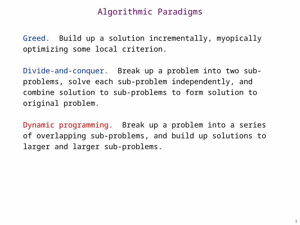
Greed. Build up a solution incrementally, myopically optimizing some local criterion.

Divide-and-conquer. Break up a problem into two sub-problems, solve each sub-problem independently, and combine solution to sub-problems to form solution to original problem.

Dynamic programming. Break up a problem into a series of overlapping sub-problems, and build up solutions to larger and larger sub-problems.

2

Dynamic Programming History

Bellman. Pioneered the systematic study of dynamic programming in the 1950s.

Etymology. Dynamic programming = planning over time. Secretary of Defense was hostile to mathematical research. Bellman sought an impressive name to avoid confrontation.

– "it's impossible to use dynamic in a pejorative sense"– "something not even a Congressman could object to"

Reference: Bellman, R. E. Eye of the Hurricane, An Autobiography.

3

Dynamic Programming Applications

Areas. Bioinformatics. Control theory. Information theory. Operations research. Computer science: theory, graphics, AI, systems, ….

Some famous dynamic programming algorithms. Viterbi for hidden Markov models. Unix diff for comparing two files. Smith-Waterman for sequence alignment. Bellman-Ford for shortest path routing in networks. Cocke-Kasami-Younger for parsing context free grammars.

6.1 Weighted Interval Scheduling

5

Weighted Interval Scheduling

Weighted interval scheduling problem. Job j starts at sj, finishes at fj, and has weight or value vj . Two jobs compatible if they don't overlap. Goal: find maximum weight subset of mutually compatible

jobs.

Time0 1 2 3 4 5 6 7 8 9 10 11

f

g

h

e

a

b

c

d

6

Unweighted Interval Scheduling Review

Recall. Greedy algorithm works if all weights are 1. Consider jobs in ascending order of finish time. Add job to subset if it is compatible with previously chosen

jobs.

Observation. Greedy algorithm can fail spectacularly if arbitrary weights are allowed.

Time0 1 2 3 4 5 6 7 8 9 10 11

b

a

weight = 999

weight = 1

7

Weighted Interval Scheduling

Notation. Label jobs by finishing time: f1 f2 . . . fn .

Def. p(j) = largest index i < j such that job i is compatible with j.

Ex: p(8) = 5, p(7) = 3, p(2) = 0.

Time0 1 2 3 4 5 6 7 8 9 10 11

6

7

8

4

3

1

2

5

8

Dynamic Programming: Binary Choice

Notation. OPT(j) = value of optimal solution to the problem consisting of job requests 1, 2, ..., j.

Case 1: OPT selects job j.– can't use incompatible jobs { p(j) + 1, p(j) + 2, ..., j - 1 }– must include optimal solution to problem consisting of

remaining compatible jobs 1, 2, ..., p(j)

Case 2: OPT does not select job j.– must include optimal solution to problem consisting of

remaining compatible jobs 1, 2, ..., j-1

optimal substructure

9

Input: n, s1,…,sn , f1,…,fn , v1,…,vn

Sort jobs by finish times so that f1 f2 ... fn.

Compute p(1), p(2), …, p(n)

Compute-Opt(j) { if (j = 0) return 0 else return max(vj + Compute-Opt(p(j)), Compute-Opt(j-1))}

Weighted Interval Scheduling: Brute Force

Brute force algorithm.

10

Weighted Interval Scheduling: Brute Force

Observation. Recursive algorithm fails spectacularly because of redundant sub-problems exponential algorithms.

Ex. Number of recursive calls for family of "layered" instances grows like Fibonacci sequence.

3

4

5

1

2

p(1) = 0, p(j) = j-2

5

4 3

3 2 2 1

2 1

1 0

1 0 1 0

11


Sort jobs by finish times so that f1 f2 ... fn.Compute p(1), p(2), …, p(n)

for j = 1 to n M[j] = emptyM[j] = 0

M-Compute-Opt(j) { if (M[j] is empty) M[j] = max(wj + M-Compute-Opt(p(j)), M-Compute-Opt(j-1)) return M[j]}

global array

Weighted Interval Scheduling: Memoization

Memoization. Store results of each sub-problem in a cache; lookup as needed.

12

Weighted Interval Scheduling: Running Time

Claim. Memoized version of algorithm takes O(n log n) time. Sort by finish time: O(n log n). Computing p() : O(n) after sorting by start time.

M-Compute-Opt(j): each invocation takes O(1) time and either– (i) returns an existing value M[j]– (ii) fills in one new entry M[j] and makes two recursive calls

Progress measure = # nonempty entries of M[].– initially = 0, throughout n. – (ii) increases by 1 at most 2n recursive calls.

Overall running time of M-Compute-Opt(n) is O(n). ▪

Remark. O(n) if jobs are pre-sorted by start and finish times.

13

Automated Memoization

Automated memoization. Many functional programming languages(e.g., Lisp) have built-in support for memoization.

Q. Why not in imperative languages (e.g., Java)?

F(40)

F(39)

F(38)

F(38)

F(37)

F(36)

F(37)

F(36) F(35)

F(36)

F(35)

F(34)

F(37)

F(36)

F(35)

static int F(int n) { if (n <= 1) return n; else return F(n-1) + F(n-2);}

(defun F (n) (if (<= n 1) n (+ (F (- n 1)) (F (- n 2)))))

Lisp (efficient)

Java (exponential)

14

Weighted Interval Scheduling: Finding a Solution

Q. Dynamic programming algorithms computes optimal value. What if we want the solution itself?A. Do some post-processing.

# of recursive calls n O(n).

Run M-Compute-Opt(n)Run Find-Solution(n)

Find-Solution(j) { if (j = 0) output nothing else if (vj + M[p(j)] > M[j-1]) print j Find-Solution(p(j)) else Find-Solution(j-1)}

15

Weighted Interval Scheduling: Bottom-Up

Bottom-up dynamic programming. Unwind recursion.


Sort jobs by finish times so that f1 f2 ... fn.

Compute p(1), p(2), …, p(n)

Iterative-Compute-Opt { M[0] = 0 for j = 1 to n M[j] = max(vj + M[p(j)], M[j-1])}

6.3 Segmented Least Squares

17

Segmented Least Squares

Least squares. Foundational problem in statistic and numerical analysis. Given n points in the plane: (x1, y1), (x2, y2) , . . . , (xn, yn). Find a line y = ax + b that minimizes the sum of the squared

error:

Solution. Calculus min error is achieved when

x

y

18


Segmented least squares. Points lie roughly on a sequence of several line segments. Given n points in the plane (x1, y1), (x2, y2) , . . . , (xn, yn) with x1 < x2 < ... < xn, find a sequence of lines that minimizes f(x).

Q. What's a reasonable choice for f(x) to balance accuracy and parsimony?

x

y

goodness of fit

number of lines

19


Segmented least squares. Points lie roughly on a sequence of several line segments. Given n points in the plane (x1, y1), (x2, y2) , . . . , (xn, yn) with x1 < x2 < ... < xn, find a sequence of lines that minimizes:

– the sum of the sums of the squared errors E in each segment

– the number of lines L Tradeoff function: E + c L, for some constant c > 0.

x

y

20

Dynamic Programming: Multiway Choice

Notation. OPT(j) = minimum cost for points p1, pi+1 , . . . , pj. e(i, j) = minimum sum of squares for points pi, pi+1 , . . . , pj.

To compute OPT(j): Last segment uses points pi, pi+1 , . . . , pj for some i. Cost = e(i, j) + c + OPT(i-1).

21

Segmented Least Squares: Algorithm

Running time. O(n3). Bottleneck = computing e(i, j) for O(n2) pairs, O(n) per pair

using previous formula.

INPUT: n, p1,…,pN , c

Segmented-Least-Squares() { M[0] = 0 for j = 1 to n for i = 1 to j compute the least square error eij for the segment pi,…, pj

for j = 1 to n M[j] = min 1 i j (eij + c + M[i-1])

return M[n]}

can be improved to O(n2) by pre-computing various statistics

6.4 Knapsack Problem

23

Knapsack Problem

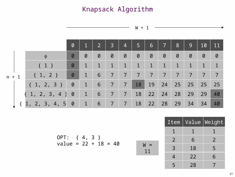
Knapsack problem. Given n objects and a "knapsack." Item i weighs wi > 0 kilograms and has value vi > 0. Knapsack has capacity of W kilograms. Goal: fill knapsack so as to maximize total value.

Ex: { 3, 4 } has value 40.

Greedy: repeatedly add item with maximum ratio vi / wi.

Ex: { 5, 2, 1 } achieves only value = 35 greedy not optimal.

1

Value

18

22

28

1

Weight

5

6

6 2

7

Item

1

3

4

5

2W = 11

24

Dynamic Programming: False Start

Def. OPT(i) = max profit subset of items 1, …, i.

Case 1: OPT does not select item i.– OPT selects best of { 1, 2, …, i-1 }

Case 2: OPT selects item i.– accepting item i does not immediately imply that we will have

to reject other items– without knowing what other items were selected before i, we

don't even know if we have enough room for i

Conclusion. Need more sub-problems!

25

Dynamic Programming: Adding a New Variable

Def. OPT(i, w) = max profit subset of items 1, …, i with weight limit w.

Case 1: OPT does not select item i.– OPT selects best of { 1, 2, …, i-1 } using weight limit w

Case 2: OPT selects item i.– new weight limit = w – wi

– OPT selects best of { 1, 2, …, i–1 } using this new weight limit

26

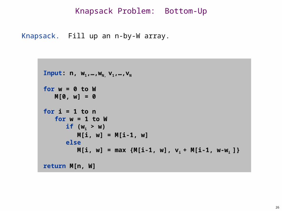
Input: n, w1,…,wN, v1,…,vN

for w = 0 to W M[0, w] = 0

for i = 1 to n for w = 1 to W if (wi > w) M[i, w] = M[i-1, w] else M[i, w] = max {M[i-1, w], vi + M[i-1, w-wi ]}

return M[n, W]

Knapsack Problem: Bottom-Up

Knapsack. Fill up an n-by-W array.

27

Knapsack Algorithm

n + 1

1

Value

18

22

28

1

Weight

5

6

6 2

7

Item

1

3

4

5

2

{ 1, 2 }

{ 1, 2, 3 }

{ 1, 2, 3, 4 }

{ 1 }

{ 1, 2, 3, 4, 5 }

0

0

0

0

0

0

0

1

0

1

1

1

1

1

2

0

6

6

6

1

6

3

0

7

7

7

1

7

4

0

7

7

7

1

7

5

0

7

18

18

1

18

6

0

7

19

22

1

22

7

0

7

24

24

1

28

8

0

7

25

28

1

29

9

0

7

25

29

1

34

10

0

7

25

29

1

34

11

0

7

25

40

1

40

W + 1

W = 11

OPT: { 4, 3 }value = 22 + 18 = 40

28

Knapsack Problem: Running Time

Running time. (n W). Not polynomial in input size! "Pseudo-polynomial." Decision version of Knapsack is NP-complete. [Chapter 8]

Knapsack approximation algorithm. There exists a polynomial algorithm that produces a feasible solution that has value within 0.01% of optimum. [Section 11.8]

6.5 RNA Secondary Structure

30

RNA Secondary Structure

RNA. String B = b1b2bn over alphabet { A, C, G, U }.

Secondary structure. RNA is single-stranded so it tends to loop back and form base pairs with itself. This structure is essential for understanding behavior of molecule.

G

U

C

A

GA

A

G

CG

A

UG

A

U

U

A

G

A

C A

A

C

U

G

A

G

U

C

A

U

C

G

G

G

C

C

G

Ex: GUCGAUUGAGCGAAUGUAACAACGUGGCUACGGCGAGA

complementary base pairs: A-U, C-G

31

RNA Secondary Structure

Secondary structure. A set of pairs S = { (bi, bj) } that satisfy: [Watson-Crick.] S is a matching and each pair in S is a Watson-

Crick complement: A-U, U-A, C-G, or G-C. [No sharp turns.] The ends of each pair are separated by at

least 4 intervening bases. If (bi, bj) S, then i < j - 4. [Non-crossing.] If (bi, bj) and (bk, bl) are two pairs in S, then we

cannot have i < k < j < l.

Free energy. Usual hypothesis is that an RNA molecule will form the secondary structure with the optimum total free energy.

Goal. Given an RNA molecule B = b1b2bn, find a secondary

structure S that maximizes the number of base pairs.

approximate by number of base pairs

32

RNA Secondary Structure: Examples

Examples.

C

G G

C

A

G

U

U

U A

A U G U G G C C A U

G G

C

A

G

U

U A

A U G G G C A U

C

G G

C

A

U

G

U

U A

A G U U G G C C A U

sharp turn crossingok

G

G

4

base pair

33

RNA Secondary Structure: Subproblems

First attempt. OPT(j) = maximum number of base pairs in a secondary structure of the substring b1b2bj.

Difficulty. Results in two sub-problems. Finding secondary structure in: b1b2bt-1. Finding secondary structure in: bt+1bt+2bn-1.

1 t n

match bt and bn

OPT(t-1)

need more sub-problems

34

Dynamic Programming Over Intervals

Notation. OPT(i, j) = maximum number of base pairs in a secondary structure of the substring bibi+1bj.

Case 1. If i j - 4.– OPT(i, j) = 0 by no-sharp turns condition.

Case 2. Base bj is not involved in a pair.

– OPT(i, j) = OPT(i, j-1)

Case 3. Base bj pairs with bt for some i t < j - 4.

– non-crossing constraint decouples resulting sub-problems– OPT(i, j) = 1 + maxt { OPT(i, t-1) + OPT(t+1, j-1) }

Remark. Same core idea in CKY algorithm to parse context-free grammars.

take max over t such that i t < j-4 andbt and bj are Watson-Crick complements

35

Bottom Up Dynamic Programming Over Intervals

Q. What order to solve the sub-problems?A. Do shortest intervals first.

Running time. O(n3).

RNA(b1,…,bn) { for k = 5, 6, …, n-1 for i = 1, 2, …, n-k j = i + k Compute M[i, j]

return M[1, n]}

using recurrence

0 0 0

0 0

02

3

4

1

i

6 7 8 9

j

36

Dynamic Programming Summary

Recipe. Characterize structure of problem. Recursively define value of optimal solution. Compute value of optimal solution. Construct optimal solution from computed information.

Dynamic programming techniques. Binary choice: weighted interval scheduling. Multi-way choice: segmented least squares. Adding a new variable: knapsack. Dynamic programming over intervals: RNA secondary structure.

Top-down vs. bottom-up: different people have different intuitions.

Viterbi algorithm for HMM also usesDP to optimize a maximum likelihoodtradeoff between parsimony and accuracy

CKY parsing algorithm for context-freegrammar has similar structure

6.6 Sequence Alignment

38

String Similarity

How similar are two strings? ocurrance occurrence

o c u r r a n c e

c c u r r e n c eo

-

o c u r r n c e

c c u r r n c eo

- - a

e -

o c u r r a n c e

c c u r r e n c eo

-

5 mismatches, 1 gap

1 mismatch, 1 gap

0 mismatches, 3 gaps

39

Applications. Basis for Unix diff. Speech recognition. Computational biology.

Edit distance. [Levenshtein 1966, Needleman-Wunsch 1970] Gap penalty ; mismatch penalty pq. Cost = sum of gap and mismatch penalties.

2 + CA

C G A C C T A C C T

C T G A C T A C A T

T G A C C T A C C T

C T G A C T A C A T

-T

C

C

C

TC + GT + AG+ 2CA

-

Edit Distance

40

Goal: Given two strings X = x1 x2 . . . xm and Y = y1 y2 . . . yn find

alignment of minimum cost.

Def. An alignment M is a set of ordered pairs xi-yj such that each

item occurs in at most one pair and no crossings.

Def. The pair xi-yj and xi'-yj' cross if i < i', but j > j'.

Ex: CTACCG vs. TACATG.Sol: M = x2-y1, x3-y2, x4-y3, x5-y4, x6-y6.

Sequence Alignment

C T A C C -

T A C A T-

G

G

y1 y2 y3 y4 y5 y6

x2 x3 x4 x5x1 x6

41

Sequence Alignment: Problem Structure

Def. OPT(i, j) = min cost of aligning strings x1 x2 . . . xi and y1 y2 . . . yj.

Case 1: OPT matches xi-yj.– pay mismatch for xi-yj + min cost of aligning two strings

x1 x2 . . . xi-1 and y1 y2 . . . yj-1 Case 2a: OPT leaves xi unmatched.

– pay gap for xi and min cost of aligning x1 x2 . . . xi-1 and y1 y2 . . . yj

Case 2b: OPT leaves yj unmatched.– pay gap for yj and min cost of aligning x1 x2 . . . xi and y1 y2 . . .

yj-1

42

Sequence Alignment: Algorithm

Analysis. (mn) time and space.English words or sentences: m, n 10.Computational biology: m = n = 100,000. 10 billions ops OK, but 10GB array?

Sequence-Alignment(m, n, x1x2...xm, y1y2...yn, , ) { for i = 0 to m M[0, i] = i for j = 0 to n M[j, 0] = j

for i = 1 to m for j = 1 to n M[i, j] = min([xi, yj] + M[i-1, j-1], + M[i-1, j], + M[i, j-1]) return M[m, n]}

6.7 Sequence Alignment in Linear Space

44

Sequence Alignment: Linear Space

Q. Can we avoid using quadratic space?

Easy. Optimal value in O(m + n) space and O(mn) time. Compute OPT(i, •) from OPT(i-1, •). No longer a simple way to recover alignment itself.

Theorem. [Hirschberg 1975] Optimal alignment in O(m + n) space and O(mn) time.

Clever combination of divide-and-conquer and dynamic programming.

Inspired by idea of Savitch from complexity theory.

45

Edit distance graph. Let f(i, j) be shortest path from (0,0) to (i, j). Observation: f(i, j) = OPT(i, j).


i-j

m-n

x1

x2

y1

x3

y2 y3 y4 y5 y6

0-0

xi y j

46

Edit distance graph. Let f(i, j) be shortest path from (0,0) to (i, j). Can compute f (•, j) for any j in O(mn) time and O(m + n)

space.


i-j

m-n

x1

x2

y1

x3

y2 y3 y4 y5 y6

0-0

j

47

Edit distance graph. Let g(i, j) be shortest path from (i, j) to (m, n). Can compute by reversing the edge orientations and inverting

the roles of (0, 0) and (m, n)


i-j

m-n

x1

x2

y1

x3

y2 y3 y4 y5 y6

0-0

xi y j

48

Edit distance graph. Let g(i, j) be shortest path from (i, j) to (m, n). Can compute g(•, j) for any j in O(mn) time and O(m + n)

space.


i-j

m-n

x1

x2

y1

x3

y2 y3 y4 y5 y6

0-0

j

49

Observation 1. The cost of the shortest path that uses (i, j) isf(i, j) + g(i, j).


i-j

m-n

x1

x2

y1

x3

y2 y3 y4 y5 y6

0-0

50

Observation 2. let q be an index that minimizes f(q, n/2) + g(q, n/2). Then, the shortest path from (0, 0) to (m, n) uses (q, n/2).


i-j

m-n

x1

x2

y1

x3

y2 y3 y4 y5 y6

0-0

n / 2

q

51

Divide: find index q that minimizes f(q, n/2) + g(q, n/2) using DP. Align xq and yn/2.

Conquer: recursively compute optimal alignment in each piece.


i-jx1

x2

y1

x3

y2 y3 y4 y5 y6

0-0

q

n / 2

m-n

52

Theorem. Let T(m, n) = max running time of algorithm on strings of length at most m and n. T(m, n) = O(mn log n).

Remark. Analysis is not tight because two sub-problems are of size(q, n/2) and (m - q, n/2). In next slide, we save log n factor.

Sequence Alignment: Running Time Analysis Warmup

53

Theorem. Let T(m, n) = max running time of algorithm on strings of length m and n. T(m, n) = O(mn).

Pf. (by induction on n) O(mn) time to compute f( •, n/2) and g ( •, n/2) and find index

q. T(q, n/2) + T(m - q, n/2) time for two recursive calls. Choose constant c so that:

Base cases: m = 2 or n = 2. Inductive hypothesis: T(m, n) 2cmn.

Sequence Alignment: Running Time Analysis

6.8 Shortest Paths

55

Shortest Paths

Shortest path problem. Given a directed graph G = (V, E), with edge weights cvw, find shortest path from node s to node t.

Ex. Nodes represent agents in a financial setting and cvw is cost of

transaction in which we buy from agent v and sell immediately to w.

s

3

t

2

6

7

45

10

18 -16

9

6

15 -8

30

20

44

16

11

6

19

6

allow negative weights

56

Shortest Paths: Failed Attempts

Dijkstra. Can fail if negative edge costs.

Re-weighting. Adding a constant to every edge weight can fail.

u

t

s v

2

1

3

-6

s t

2

3

2

-3

3

5 5

66

0

57

Shortest Paths: Negative Cost Cycles

Negative cost cycle.

Observation. If some path from s to t contains a negative cost cycle, there does not exist a shortest s-t path; otherwise, there exists one that is simple.

s tW

c(W) < 0

-6

7

-4

58

Shortest Paths: Dynamic Programming

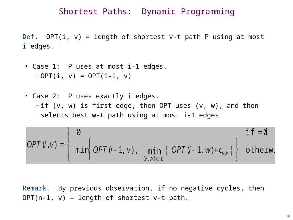
Def. OPT(i, v) = length of shortest v-t path P using at most i edges.

Case 1: P uses at most i-1 edges.– OPT(i, v) = OPT(i-1, v)

Case 2: P uses exactly i edges.– if (v, w) is first edge, then OPT uses (v, w), and then selects

best w-t path using at most i-1 edges

Remark. By previous observation, if no negative cycles, thenOPT(n-1, v) = length of shortest v-t path.

59

Shortest Paths: Implementation

Analysis. (mn) time, (n2) space.

Finding the shortest paths. Maintain a "successor" for each table entry.

Shortest-Path(G, t) { foreach node v V M[0, v] M[0, t] 0

for i = 1 to n-1 foreach node v V M[i, v] M[i-1, v] foreach edge (v, w) E M[i, v] min { M[i, v], M[i-1, w] + cvw }}

60

Shortest Paths: Practical Improvements

Practical improvements. Maintain only one array M[v] = shortest v-t path that we have

found so far. No need to check edges of the form (v, w) unless M[w] changed

in previous iteration.

Theorem. Throughout the algorithm, M[v] is length of some v-t path, and after i rounds of updates, the value M[v] is no larger than the length of shortest v-t path using i edges.

Overall impact. Memory: O(m + n). Running time: O(mn) worst case, but substantially faster in

practice.

61

Bellman-Ford: Efficient Implementation

Push-Based-Shortest-Path(G, s, t) { foreach node v V { M[v] successor[v] }

M[t] = 0 for i = 1 to n-1 { foreach node w V { if (M[w] has been updated in previous iteration) { foreach node v such that (v, w) E { if (M[v] > M[w] + cvw) { M[v] M[w] + cvw successor[v] w } } } If no M[w] value changed in iteration i, stop. }}

6.9 Distance Vector Protocol

63

Distance Vector Protocol

Communication network. Nodes routers. Edges direct communication link. Cost of edge delay on link.

Dijkstra's algorithm. Requires global information of network.

Bellman-Ford. Uses only local knowledge of neighboring nodes.

Synchronization. We don't expect routers to run in lockstep. The order in which each foreach loop executes in not important. Moreover, algorithm still converges even if updates are asynchronous.

naturally nonnegative, but Bellman-Ford used anyway!

64

Distance Vector Protocol

Distance vector protocol. Each router maintains a vector of shortest path lengths to

every other node (distances) and the first hop on each path (directions).

Algorithm: each router performs n separate computations, one for each potential destination node.

"Routing by rumor."

Ex. RIP, Xerox XNS RIP, Novell's IPX RIP, Cisco's IGRP, DEC's DNA Phase IV, AppleTalk's RTMP.

Caveat. Edge costs may change during algorithm (or fail completely).

tv 1s 1

1

deleted

"counting to infinity"

2 1

65

Path Vector Protocols

Link state routing. Each router also stores the entire path. Based on Dijkstra's algorithm. Avoids "counting-to-infinity" problem and related difficulties. Requires significantly more storage.

Ex. Border Gateway Protocol (BGP), Open Shortest Path First (OSPF).

not just the distance and first hop

6.10 Negative Cycles in a Graph

67

Detecting Negative Cycles

Lemma. If OPT(n,v) = OPT(n-1,v) for all v, then no negative cycles.Pf. Bellman-Ford algorithm.

Lemma. If OPT(n,v) < OPT(n-1,v) for some node v, then (any) shortest path from v to t contains a cycle W. Moreover W has negative cost.

Pf. (by contradiction) Since OPT(n,v) < OPT(n-1,v), we know P has exactly n edges. By pigeonhole principle, P must contain a directed cycle W. Deleting W yields a v-t path with < n edges W has negative

cost.

v tW

c(W) < 0

68

Detecting Negative Cycles

Theorem. Can detect negative cost cycle in O(mn) time. Add new node t and connect all nodes to t with 0-cost edge. Check if OPT(n, v) = OPT(n-1, v) for all nodes v.

– if yes, then no negative cycles– if no, then extract cycle from shortest path from v to t

v

18

2

5 -23

-15 -11

6

t

0

0

0 0

0

69

Detecting Negative Cycles: Application

Currency conversion. Given n currencies and exchange rates between pairs of currencies, is there an arbitrage opportunity?

Remark. Fastest algorithm very valuable!

F$

£ ¥DM

1/7

3/102/3 2

170 56

3/504/3

8

IBM

1/10000

800

70

Detecting Negative Cycles: Summary

Bellman-Ford. O(mn) time, O(m + n) space. Run Bellman-Ford for n iterations (instead of n-1). Upon termination, Bellman-Ford successor variables trace a

negative cycle if one exists. See p. 288 for improved version and early termination rule.

algorithmic paradigms

Documents

jobs compatible

remaining compatible

vnsort jobs

selects job j

pnfor j

incompatible jobs

chosen jobs

label jobs