algorithmics: basic de nitions and concepts
TRANSCRIPT
The course
Algorithms:our context
Timecomplexity
Asymptoticnotation
Graphs
Data structures
Traversals
Reductions
Divide andconquer
Algorithmics: Basic definitions and concepts

The course
Algorithms:our context
Timecomplexity
Asymptoticnotation
Graphs
Data structures
Traversals
Reductions
Divide andconquer
The Algorithmics course
Already known (nivell EDA)
Algorithms cost and Asymptotic notation
Sorting algorithms: Mergesort, Quicksort, . . .
Divide and conquer, recurrences, master theorem
Complexity, P and NP, reductions
Foundations on probability
Basic data structures: Arrays, lists, stacks, queues, heaps,hashing . . .
Basics on graph theory, graph data structures
Graph and digrah traversals (BFS, DFS) and applications.
Backtracking algorithms

The course
Algorithms:our context
Timecomplexity
Asymptoticnotation
Graphs
Data structures
Traversals
Reductions
Divide andconquer
The Algorithmics course
Topics to cover:
Divide and conquer: Linear Selection
Sorting in linear time
Greedy algorithms
Dynamic programming
Distances in graphs
Flow networks: problems, algorithms and applications
Linear Programming
Approximation algorithms
Provide models to solve real problems
The course
Algorithms:our context
Timecomplexity
Asymptoticnotation
Graphs
Data structures
Traversals
Reductions
Divide andconquer
References
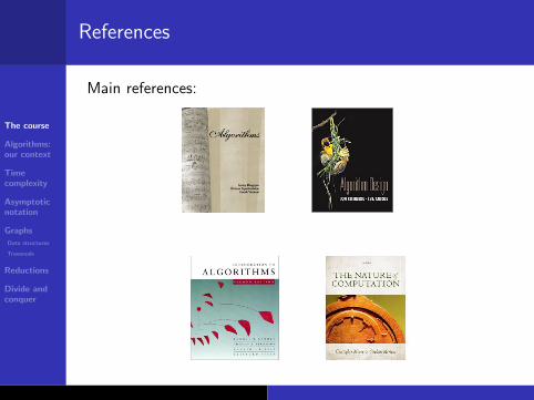
Main references:

The course
Algorithms:our context
Timecomplexity
Asymptoticnotation
Graphs
Data structures
Traversals
Reductions
Divide andconquer
”The algorithmic lenses: C. Papadimitriou”
In 1936 Alan Turing demonstrated the universality ofcomputational principles with his mathematical model ofthe Turing machine.
Theoretical Computer Science views computation as aubiquitous phenomenon, not one that it is limited tocomputers.
Algorithms themselves have evolved into a complex set oftechniques, for instances self-learning, Web services,concurrent, distributed or parallel, etc... Each of themwith ad-hoc relevant computational limitations and socialimplications.
However, this course will be a course on classicalalgorithms, which are the core needed to understand moreadvanced computational material.

The course
Algorithms:our context
Timecomplexity
Asymptoticnotation
Graphs
Data structures
Traversals
Reductions
Divide andconquer
Algorithms
Algorithm: Precise recipe for a precise computational task.Each step of the process must be clear and unambiguous, andit should always yield a clear answer.
Sqrt (n)x0 = 1for i = 1 to 6 do
xi = (xi−1 + n/xi−1)/2end for
Babilonia (XVI BC)For n = 20, x ’s are 1 10.5 6.2023 4.7134 4.4783
The course
Algorithms:our context
Timecomplexity
Asymptoticnotation
Graphs
Data structures
Traversals
Reductions
Divide andconquer
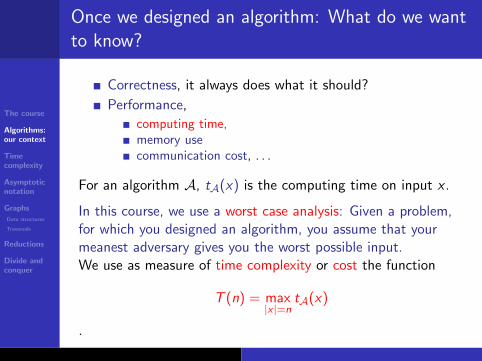
Once we designed an algorithm: What do we wantto know?
Correctness, it always does what it should?
Performance,
computing time,memory usecommunication cost, . . .
For an algorithm A, tA(x) is the computing time on input x .
In this course, we use a worst case analysis: Given a problem,for which you designed an algorithm, you assume that yourmeanest adversary gives you the worst possible input.We use as measure of time complexity or cost the function
T (n) = max|x |=n
tA(x)
.

The course
Algorithms:our context
Timecomplexity
Asymptoticnotation
Graphs
Data structures
Traversals
Reductions
Divide andconquer
Time complexity
The time complexity must be independent of the ”used”machine
We must consider carefully how operations scale with respectto size.
The course
Algorithms:our context
Timecomplexity
Asymptoticnotation
Graphs
Data structures
Traversals
Reductions
Divide andconquer
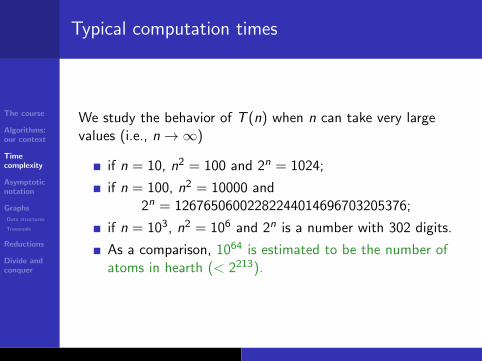
Typical computation times
We study the behavior of T (n) when n can take very largevalues (i.e., n→∞)
if n = 10, n2 = 100 and 2n = 1024;
if n = 100, n2 = 10000 and2n = 12676506002282244014696703205376;
if n = 103, n2 = 106 and 2n is a number with 302 digits.
As a comparison, 1064 is estimated to be the number ofatoms in hearth (< 2213).

The course
Algorithms:our context
Timecomplexity
Asymptoticnotation
Graphs
Data structures
Traversals
Reductions
Divide andconquer
Computation time assuming that an input with sizen = 1 can be solved in 1 µsecond:
26 THE BASICS
100
103
106
109
1012
1015
1018
1021
1024
0 10 20 30 40 50 60 70 80 90 100n
µs
n
n 2
n 3
2n
n !
1 minute
1 day
1 year
age of universe
FIGURE 2.5: Running times of algorithms as a function of the size n . We assume that each one can solvean instance of size n = 1 in one microsecond. Note that the time axis is logarithmic.
Eulerinput: a graph G = (V, E )output: “yes” if G is Eulerian, and “no” otherwisebegin
y := 0 ;for all v ∈V do
if deg(v ) is odd then y := y +1;if y > 2 then return “no”;
endreturn “yes”
end
FIGURE 2.6: Euler’s algorithm for EULERIAN PATH. The variable y counts the number of odd-degree vertices.
2.4.2 Details, and Why they Don’t Matter
In the Prologue we saw that Euler’s approach to EULERIAN PATH is much more efficient than exhaustivesearch. But how does the running time of the resulting algorithm scale with the size of the graph? It turnsout that a precise answer to this question depends on many details. We will discuss just enough of thesedetails to convince you that we can and should ignore them in our quest for a fundamental understandingof computational complexity.
From: Moore-Mertens, The Nature of Computation

The course
Algorithms:our context
Timecomplexity
Asymptoticnotation
Graphs
Data structures
Traversals
Reductions
Divide andconquer
Computation times as a function of input size n
n n lg n n2 1.5n 2n
10 < 1s < 1s < 1s < 1s < 1s50 < 1s < 1s < 1s 11m 36y
100 < 1s < 1s < 1s 12000y 1017y1000 < 1s < 1s < 1s > 1025y > 1025y104 < 1s < 1s < 1s > 1025y > 1025y105 < 1s < 1s < 1s > 1025y > 1025y106 < 1s 20s 12d > 1025y > 1025y
From: Moore-Mertens, The Nature of Computation

The course
Algorithms:our context
Timecomplexity
Asymptoticnotation
Graphs
Data structures
Traversals
Reductions
Divide andconquer
Efficient algorithms and practical algorithms
When analyzing an algorithm, we say that it is feasible ifits cost is polynomial.n10
10is a polynomial but this computing time could be
prohibitive!
In the same way, if we have cn2 for constant c = 1064,then c dominates inputs up to a size of n > 1064.
In this course, we will not enter in the analysis up toconstants, but keep in mind that constants matter!!!!
In practice, even for feasible algorithms with timecomplexity of for example n4, it could be too slow forn ≥ 1000.

The course
Algorithms:our context
Timecomplexity
Asymptoticnotation
Graphs
Data structures
Traversals
Reductions
Divide andconquer
Asymptotic notation
Symbol L = limn→∞f (n)g(n) intuition
f (n) = O(g(n)) L <∞ f ≤ g
f (n) = Ω(g(n)) L > 0 f ≥ g
f (n) = Θ(g(n)) 0 < L <∞ f = g
f (n) = o(g(n)) L = 0 f < g
f (n) = ω(g(n)) L =∞ f > g
The course
Algorithms:our context
Timecomplexity
Asymptoticnotation
Graphs
Data structures
Traversals
Reductions
Divide andconquer
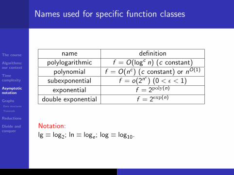
Names used for specific function classes
name definition
polylogarithmic f = O(logc n) (c constant)
polynomial f = O(nc) (c constant) or nO(1)
subexponential f = o(2nε) (0 < ε < 1)
exponential f = 2poly(n)
double exponential f = 2exp(n)
Notation:lg ≡ log2; ln ≡ loge ; log ≡ log10.

The course
Algorithms:our context
Timecomplexity
Asymptoticnotation
Graphs
Data structures
Traversals
Reductions
Divide andconquer
Some math. you should remember
Given an integer n > 0 and a real a > 1 and a 6= 0:
Arithmetic summation:∑n
i=0 i = n(n+1)2 .
Geometric summation:∑n
i=0 ai = 1−an+1
1−a .
Logarithms and Exponents: For a, b, c ∈ R+,
logb a = c ⇔ a = bc ⇒ logb 1 = 0
logb ac = logb a + logb c , logb a/c = logb a− logb c.
logb ac = c logb a ⇒ c logb a = alogb c ⇒ 2log2 n = n.
logb a = logc a/ logc b ⇒ logb a = Θ(logc a)
Stirling: n! =√
2πn(n/e)n + 0(1/n) + γ ⇒ n! + ω((n/2)n).
n-Harmonic: Hn =∑n
i=1 1/i ∼ ln n.

The course
Algorithms:our context
Timecomplexity
Asymptoticnotation
Graphs
Data structures
Traversals
Reductions
Divide andconquer
Graphs
See for ex. Chapter 3 of Dasgupta, Papadimitriou, Vazirani (DPV).
Graph: G = (V ,E ), where V is the set of vertices, n = |V |,and E ⊂ V × V is the set of edges, m = |E |,
Graphs: undirected graphs (graphs) and directed graphs(digraphs)
The degree of v (d(v)) is the number of edges which areincident to v .
A clique on n vertices (Kn) is a complete graph (withm = n(n − 1)/2).
A undirected G is said to be connected if there is a pathbetween any two distinct vertices.
If G is connected, then m ≥ n − 1.
The course
Algorithms:our context
Timecomplexity
Asymptoticnotation
Graphs
Data structures
Traversals
Reductions
Divide andconquer
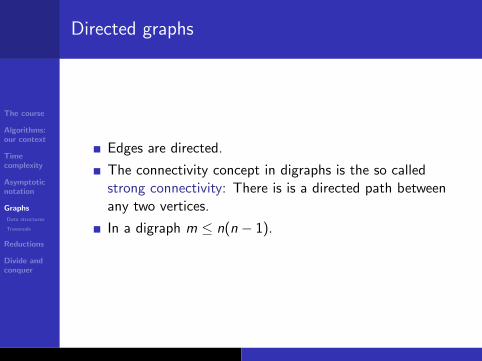
Directed graphs
Edges are directed.
The connectivity concept in digraphs is the so calledstrong connectivity: There is is a directed path betweenany two vertices.
In a digraph m ≤ n(n − 1).

The course
Algorithms:our context
Timecomplexity
Asymptoticnotation
Graphs
Data structures
Traversals
Reductions
Divide andconquer
Density of a graph
A G with n vertices is said to be dense when m = Θ(n2).When m = o(n2), G is said to be sparse.

The course
Algorithms:our context
Timecomplexity
Asymptoticnotation
Graphs
Data structures
Traversals
Reductions
Divide andconquer
Common graph’s data structures
Let G be a graph with V = 1, 2, . . . , n.
Adjacency list
Adjacency matrix

The course
Algorithms:our context
Timecomplexity
Asymptoticnotation
Graphs
Data structures
Traversals
Reductions
Divide andconquer
Adjacency list
c
a
b
c
d
b d
a d c
d b
a b c
a
a
b
b c
d
d
c
a
b
c
d
a
b
d
c

The course
Algorithms:our context
Timecomplexity
Asymptoticnotation
Graphs
Data structures
Traversals
Reductions
Divide andconquer
Adjacency matrix
Given G with |V | = n define its adjacency matrix as the n × nmatrix:
A[i , j ] =
1 if (i , j) ∈ E ,
0 if (i , j) 6∈ E .
c
a
a
b
b c
d
d
abcd
a b c d0 1 0 11 0 1 10 1 0 11 1 1 0
abcd
a b c d0 0 0 11 0 1 00 0 0 00 1 1 0

The course
Algorithms:our context
Timecomplexity
Asymptoticnotation
Graphs
Data structures
Traversals
Reductions
Divide andconquer
Adjacency matrix
If G is undirected, its adjacency matrix A(G ) is symmetric.
If A is the adjacency matrix of G , then A2 gives, fori , j ∈ V , whether there is a path between i and j in G ,with length 2.For k > 0, Ak indicates if there is a path with length k inG .
If G has weights on edges, i.e. wi ,j for each (i , j) ∈ E ,A(G ) has wij in ai ,j .
Adjacency matrix allows the use of tools from linearalgebra.

The course
Algorithms:our context
Timecomplexity
Asymptoticnotation
Graphs
Data structures
Traversals
Reductions
Divide andconquer
Comparison between the matrix and the list DS
The adjacency list uses a register per vertex and two peredge. As each register needs 64 bits, then the space torepresent a graph is Θ(n + m).
The use of the adjacency matrix needs n2 bits (0, 1), sofor an unweighted graph G , we need Θ(n2) bits.
For weighted G , we need 64n2 bits (assuming weights arereasonably “small”).
In general, for unweighted dense graphs, the adjacencymatrix is better, otherwise the adjacency list is a shorterrepresentation.

The course
Algorithms:our context
Timecomplexity
Asymptoticnotation
Graphs
Data structures
Traversals
Reductions
Divide andconquer
Complexity issues between matrix and list DS
Adding a new edge to G : In both data structures we needΘ(1).
Edge query, for u and v in V (G ), (u, v) ∈ E (V )?:For matrix representation: Θ(1).For list representation: O(n).
Explore all neighbours of vertex v :For matrix representation: Θ(n)For list representation: Θ(|d(v)|)Erase an edge in G : The same as Edge query.
Erase a vertex in G :For matrix representation: Θ(n).For list representation: O(m).

The course
Algorithms:our context
Timecomplexity
Asymptoticnotation
Graphs
Data structures
Traversals
Reductions
Divide andconquer
Searching a graph: Breadth First Search
1 Start with vertex v , visit vand all its neighbors.
2 Then, the non-visitedneighbors of visited ones.
3 Repeat until all vertices arevisited.
BFS use a QUEUE, (FIFO) to keep the neighbors of visitedvertices.
Recall that vertices are labeled to avoid visiting them morethan once.

The course
Algorithms:our context
Timecomplexity
Asymptoticnotation
Graphs
Data structures
Traversals
Reductions
Divide andconquer
Searching a graph: Depth First Search
explore
1 From current vertex, move to aneighbor.
2 Until you get stuck.
3 Then backtrack till new place toexplore.
DFS use a STACK, (LIFO)
The course
Algorithms:our context
Timecomplexity
Asymptoticnotation
Graphs
Data structures
Traversals
Reductions
Divide andconquer
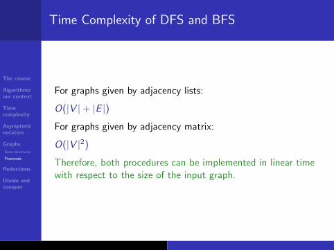
Time Complexity of DFS and BFS
For graphs given by adjacency lists:
O(|V |+ |E |)
For graphs given by adjacency matrix:
O(|V |2)
Therefore, both procedures can be implemented in linear timewith respect to the size of the input graph.

The course
Algorithms:our context
Timecomplexity
Asymptoticnotation
Graphs
Data structures
Traversals
Reductions
Divide andconquer
Connected components in undirected graphs
A connected component is a maximal connected subgraph of G .
A connected graph has a unique connected component.
Connected ComponentsINPUT: undirected graph GQUESTION: Find all the connected components of G .
To find connected componentsin G use DFS and keep trackof the set of vertices visited ineach explore call.
a
b
c
de
f
g
hi
The problem can be solved in O(|V |+ |E |).
The course
Algorithms:our context
Timecomplexity
Asymptoticnotation
Graphs
Data structures
Traversals
Reductions
Divide andconquer
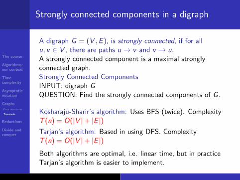
Strongly connected components in a digraph
A digraph G = (V ,E ), is strongly connected, if for allu, v ∈ V , there are paths u → v and v → u.A strongly connected component is a maximal stronglyconnected graph.Strongly Connected ComponentsINPUT: digraph GQUESTION: Find the strongly connected components of G .
Kosharaju-Sharir’s algorithm: Uses BFS (twice). ComplexityT (n) = O(|V |+ |E |)Tarjan’s algorithm: Based in using DFS. ComplexityT (n) = O(|V |+ |E |)
Both algorithms are optimal, i.e. linear time, but in practiceTarjan’s algorithm is easier to implement.

The course
Algorithms:our context
Timecomplexity
Asymptoticnotation
Graphs
Data structures
Traversals
Reductions
Divide andconquer
Strongly connected components in a digraph
A nice property: For every digraph, the graph on its stronglyconnected components is acyclic.
a b c
d e f
g h i
j lk
a, b, e
d c, f , h
g , j , k , l i

The course
Algorithms:our context
Timecomplexity
Asymptoticnotation
Graphs
Data structures
Traversals
Reductions
Divide andconquer
The classes P and NP
Recall that a problem belong to the class P if there existsan algorithm that is polynomial in the worst-case analysis,(for the worst input given by a malicious adversary)
A problem given in decisional form belong to the class NPnon-deterministic polynomial time if given a certificate ofa solution we can verify in polynomial time that indeed thecertificate is a valid solution to the problem in decisionalform and those certificates have polynomial size
It is easy to se that P⊆ NP, but it is an open problem toprove that P=NP or that P6=NP.
The class NP-complete is the class of most difficultproblems in decisional form that are in NP. Most difficultin the sense that if one of them is proved to be in P thenP=NP.
The course
Algorithms:our context
Timecomplexity
Asymptoticnotation
Graphs
Data structures
Traversals
Reductions
Divide andconquer
Beyond worst-case analysis
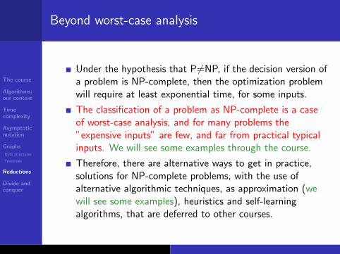
Under the hypothesis that P6=NP, if the decision version ofa problem is NP-complete, then the optimization problemwill require at least exponential time, for some inputs.
The classification of a problem as NP-complete is a caseof worst-case analysis, and for many problems the”expensive inputs” are few, and far from practical typicalinputs. We will see some examples through the course.
Therefore, there are alternative ways to get in practice,solutions for NP-complete problems, with the use ofalternative algorithmic techniques, as approximation (wewill see some examples), heuristics and self-learningalgorithms, that are deferred to other courses.

The course
Algorithms:our context
Timecomplexity
Asymptoticnotation
Graphs
Data structures
Traversals
Reductions
Divide andconquer
A powerful tool to solve problems: Reductions
You have been introduced in previous courses to the concept ofreduction between decision problems, to define the classNP-complete.
We have to extend the concept to function problems.

The course
Algorithms:our context
Timecomplexity
Asymptoticnotation
Graphs
Data structures
Traversals
Reductions
Divide andconquer
Reductions
Given problems A and B, assume we have an algorithm AB tosolve the problem B on any input y .
A polynomial time reduction A ≤ B is a pair of polynomialtime functions (f , g) such that
f maps any input x to A, in polynomial time to an inputf (x) to problem B in such a way that x has a validsolution for A iff f (x) has a valid solution for B.
g maps solutions to f (x) into solutions to x .
Therefore if we have that A ≤ B, as there is an algorithm AB
to solve problem B in polynomial time, then we have analgorithm AA, for any input x of A: Compute g(AB(f (x))),that runs in polynomial time.

The course
Algorithms:our context
Timecomplexity
Asymptoticnotation
Graphs
Data structures
Traversals
Reductions
Divide andconquer
The Vertex Cover problem
Vertex Cover: Given a graph G = (V ,E ) with|V | = n, |E | = m, find the minimum set of vertices S ⊆ V suchthat it covers every edge of G .Example:
The Vertex Cover problem is known to be in NP-hard.

The course
Algorithms:our context
Timecomplexity
Asymptoticnotation
Graphs
Data structures
Traversals
Reductions
Divide andconquer
The Set Cover problem
Set Cover: Given a set U of m elements, a collectionS = S1, . . . ,Sn where each Si ⊆ U, select de minimumnumber of subsets in such a way that their union is equal to U.
There is a weighted version of the problem, but this simplerversion already is NP-hard.
Example: Given U = 1, 2, 3, 4, 5, 6, 7 (m = 7), with Sa = 3, 7,Sb = 2, 4, Sc = 3, 4, 5, 6, Sd = 6, Se = 1, Sf = 1, 2, 6, 7.
Solution: Sc , Sf U
1 2
5
6
4
37

The course
Algorithms:our context
Timecomplexity
Asymptoticnotation
Graphs
Data structures
Traversals
Reductions
Divide andconquer
Set Cover
The Vertex Cover problem is a special case of the SetCover problem. As a model, the Set Cover has importantpractical applications.To understand the computational complexity of Set Cover itis important to understand first the complexity of special casesas Vertex Cover.

The course
Algorithms:our context
Timecomplexity
Asymptoticnotation
Graphs
Data structures
Traversals
Reductions
Divide andconquer
Vertex Cover ≤ Set Cover
Given a input to Vertex Cover G = (V ,E ), of size|V |+ |E | = n + m we want to construct in polynomial time onn + m a specific input f (G ) = (U,S) to Set Cover such thatif there exist a polynomial algorithm A to find a min. vertexcover in G , then A(f (G )) is an efficient algorithm to find anoptimal solution to set cover.
REDUCTION f :
Consider U as the set E of edges.
For each vertex i ∈ V , Si is the set of edges incident to i .Therefore |S | = n and for each Si , |Si | ≤ m.
The cost of the reduction from G to (U, S) is O(n + m)

The course
Algorithms:our context
Timecomplexity
Asymptoticnotation
Graphs
Data structures
Traversals
Reductions
Divide andconquer
Example for the reduction
7
a b
c
de
f
1
23 4
5
6
f︷︸︸︷⇒U = 1, 2, 3, 4, 5, 6, 7S = Sa,Sb,Sc , Sd ,Se , Sf Sa = 3, 7, Sb = 3, 7,Sc = 3, 4, 5, 6, Sd = 5,Se = 1, Sf = 1, 2, 6, 7.
If there is an algorithm to solve the Set Cover for G , thesame algorithm apply to (U, S) = f (G ) will yield a solution forVertex Cover on input (U,V ).
But both Vertex Cover and Set Cover are known to beNP-hard.
The course
Algorithms:our context
Timecomplexity
Asymptoticnotation
Graphs
Data structures
Traversals
Reductions
Divide andconquer
The divide-and-conquer strategy.
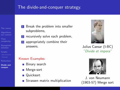
1 Break the problem into smallersubproblems,
2 recursively solve each problem,
3 appropriately combine theiranswers. Julius Caesar (I-BC)
”Divide et impera”
Known Examples:
Binary search
Merge-sort
Quicksort
Strassen matrix multiplicationJ. von Neumann
(1903-57) Merge sort

The course
Algorithms:our context
Timecomplexity
Asymptoticnotation
Graphs
Data structures
Traversals
Reductions
Divide andconquer
Recurrences Divide and Conquer
T (n) = 3T (n/2) + O(n)The algorithm under analysis divides input of size n into 3subproblems, each of size n/2, at a cost (of dividing andjoining the solutions) of O(n)
n/4
1 1 1 1 1 1
size n
n/2n/2n/2
n/4 n/4 n/4 n/4 n/4 n/4 n/4 n/4

The course
Algorithms:our context
Timecomplexity
Asymptoticnotation
Graphs
Data structures
Traversals
Reductions
Divide andconquer
T (n) = 3T (n/2) + O(n).
3
1 1 1
k=0
k=1
k=2
k=lg n
lg n
size n
T(n)=3T(n/2)+O(n)
n/2 n/2 n/2
n/4 n/4
27/8n
9/4n
3/2n
n
n/4 n/4 n/4
lg n
n/4n/4n/4n/4
The course
Algorithms:our context
Timecomplexity
Asymptoticnotation
Graphs
Data structures
Traversals
Reductions
Divide andconquer
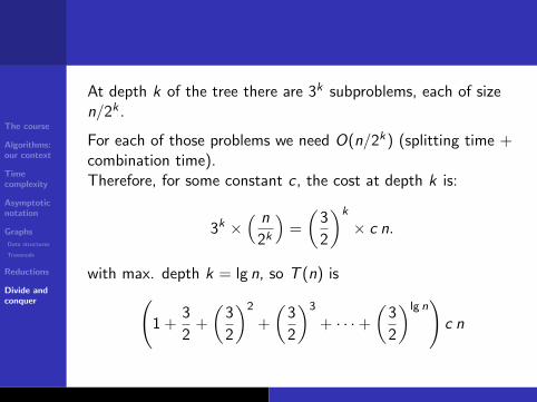
At depth k of the tree there are 3k subproblems, each of sizen/2k .
For each of those problems we need O(n/2k) (splitting time +combination time).Therefore, for some constant c , the cost at depth k is:
3k ×( n
2k
)=
(3
2
)k
× c n.
with max. depth k = lg n, so T (n) is(1 +
3
2+
(3
2
)2
+
(3
2
)3
+ · · ·+(
3
2
)lg n)c n

The course
Algorithms:our context
Timecomplexity
Asymptoticnotation
Graphs
Data structures
Traversals
Reductions
Divide andconquer
From T (n) = c n(∑lg n
k=0
(32
)k),
We have a geometric series of ratio 3/2, starting at 1 and
ending at((32)lg n
)= nlg 3
nlg 2 = n1.58
n = n0.58.
As the series is increasing, T (n) is dominated by the last term:
T (n) = c n
(nlg 3
n
)= O(n1.58).

The course
Algorithms:our context
Timecomplexity
Asymptoticnotation
Graphs
Data structures
Traversals
Reductions
Divide andconquer
A basic Master Theorem
There are several versions of the Master Theorem to solveD&C recurrences. The one presented below is taken fromDPV’s book.
Theorem (DPV-2.2)
If T (n) = aT (dn/be) + O(nd) for constantsa ≥ 1, b > 1, d ≥ 0, then has asymptotic solution:
T (n) =
O(nd), if d > logb a,
O(nd lg n), if d = logb a,
O(nlogb a), if d < logb a.
The course
Algorithms:our context
Timecomplexity
Asymptoticnotation
Graphs
Data structures
Traversals
Reductions
Divide andconquer
Master Theorems
This basic Master Theorem does not provide always exactboundsA different one can be found in CLRS’s book providing exactbounds but leaving cases outside.For stronger versions:Akra-Bazi Theorem: https:
//courses.csail.mit.edu/6.046/spring04/handouts/akrabazzi.pdf
Salvador Roura Theorems
http://www.lsi.upc.edu/~diaz/RouraMT.pdf