algorithms and analysis for underwater vehicle plume tracing
TRANSCRIPT
SANDIA REPORT
SAND2003-2643 Unlimited Release Printed July 2003 Algorithms and Analysis for Underwater Vehicle Plume Tracing
Raymond H. Byrne, Steven E. Eskridge, John E. Hurtado and Elizabeth L. Savage
Prepared by Sandia National Laboratories Albuquerque, New Mexico 87185 and Livermore, California 94550 Sandia is a multiprogram laboratory operated by Sandia Corporation, a Lockheed Martin Company, for the United States Department of Energy’s National Nuclear Security Administration under Contract DE-AC04-94AL85000. Approved for public release; further dissemination unlimited.

Issued by Sandia National Laboratories, operated for the United States Department of Energy by Sandia Corporation.
NOTICE: This report was prepared as an account of work sponsored by an agency of the United States Government. Neither the United States Government, nor any agency thereof, nor any of their employees, nor any of their contractors, subcontractors, or their employees, make any warranty, express or implied, or assume any legal liability or responsibility for the accuracy, completeness, or usefulness of any information, apparatus, product, or process disclosed, or represent that its use would not infringe privately owned rights. Reference herein to any specific commercial product, process, or service by trade name, trademark, manufacturer, or otherwise, does not necessarily constitute or imply its endorsement, recommendation, or favoring by the United States Government, any agency thereof, or any of their contractors or subcontractors. The views and opinions expressed herein do not necessarily state or reflect those of the United States Government, any agency thereof, or any of their contractors. Printed in the United States of America. This report has been reproduced directly from the best available copy. Available to DOE and DOE contractors from
U.S. Department of Energy Office of Scientific and Technical Information P.O. Box 62 Oak Ridge, TN 37831 Telephone: (865)576-8401 Facsimile: (865)576-5728 E-Mail: [email protected] Online ordering: http://www.doe.gov/bridge
Available to the public from
U.S. Department of Commerce National Technical Information Service 5285 Port Royal Rd Springfield, VA 22161 Telephone: (800)553-6847 Facsimile: (703)605-6900 E-Mail: [email protected] Online order: http://www.ntis.gov/help/ordermethods.asp?loc=7-4-0#online
2
SAND2003-2643Unlimited ReleasePrinted July 2003
ALGORITHMS AND ANALYSIS FORUNDERWATER VEHICLE PLUME TRACING
Raymond H. Byrne and Steven E. EskridgeSandia National LaboratoriesMS 0501, PO Box 5800
Albuquerque, NM 87185-0501email: [email protected]
John E. Hurtado and Elizabeth L. SavageDepartment of Aerospace Engineering
Texas A&M UniversityCollege Station, TX 77843-3141email: [email protected]
Abstract
The goal of this research was to develop and demonstrate cooperative 3-D plumetracing algorithms for miniature autonomous underwater vehicles. Applications for thistechnology include Lost Asset and Survivor Location Systems (L-SALS) and Ship-in-Port Patrol and Protection (SP3). This research was a joint effort that included NektonResearch, LLC, Sandia National Laboratories, and Texas A&M University. NektonResearch developed the miniature autonomous underwater vehicles while Sandia andTexas A&M developed the 3-D plume tracing algorithms. This report describes theplume tracing algorithm and presents test results from successful underwater testingwith pseudo-plume sources.
This work was funded by the Defense Advanced ResearchProjects Agency (DARPA) under contract DE-AC04-94AL85000
3
Contents
List of Figures 6
1 Introduction 8
2 3-D Plume Tracing Algorithm 8
2.1 Determining the Unknown Coefficients for Ill-Conditioned Cases - MethodI . . . . . . . . . . . . . . . . . . . . . . . . . . . . . . . . . . . . . . . . 11
2.2 Determining the Unknown Coefficients for Ill-Conditioned Cases - MethodII . . . . . . . . . . . . . . . . . . . . . . . . . . . . . . . . . . . . . . . . 12
3 Modeling of Light Data 12
4 Standard MATLAB Simulation Code 13
5 Sensor Measurement Dependence on Vehicle Orientation 13
6 Sensor Measurement Noise 16
7 Robot Position Error 22
8 Navigational Error 22
9 Software Implementation 26
10 Test Results 27
11 Summary 29
12 Acknowledgments 34
4
A MATLAB M-FILES 36
A.1 batchsimu.m . . . . . . . . . . . . . . . . . . . . . . . . . . . . . . . . . 36
A.2 getneighbors.m . . . . . . . . . . . . . . . . . . . . . . . . . . . . . . . . 36
A.3 getnewpos.m . . . . . . . . . . . . . . . . . . . . . . . . . . . . . . . . . 36
A.4 getupdate.m . . . . . . . . . . . . . . . . . . . . . . . . . . . . . . . . . . 37
A.5 input r2.m . . . . . . . . . . . . . . . . . . . . . . . . . . . . . . . . . . . 38
A.6 input r2depend.m . . . . . . . . . . . . . . . . . . . . . . . . . . . . . . . 39
A.7 local3D.m . . . . . . . . . . . . . . . . . . . . . . . . . . . . . . . . . . . 40
A.8 Local3DSN.m . . . . . . . . . . . . . . . . . . . . . . . . . . . . . . . . . 43
A.9 plotcompare.m . . . . . . . . . . . . . . . . . . . . . . . . . . . . . . . . 46
A.10 r2depend.m . . . . . . . . . . . . . . . . . . . . . . . . . . . . . . . . . . 48
A.11 r2.m . . . . . . . . . . . . . . . . . . . . . . . . . . . . . . . . . . . . . . 48
5
List of Figures
1 Miniature Robotic Vehicle . . . . . . . . . . . . . . . . . . . . . . . . . . 9
2 Nekton Research, LLC Miniature Autonomous Underwater Vehicle . . . 9
3 Typical result from Local3D.m. The source is located at (xs, ys, zs) =(0, 0, 0). Ten robots cooperate to localize the source. Six of the ten robotshave converged upon the source after 25 update steps. . . . . . . . . . . 14
4 This illustration shows the dependence of a light sensor measurement onvehicle orientation. . . . . . . . . . . . . . . . . . . . . . . . . . . . . . . 15
5 Position updates of ten robots. Black traces correspond to sensor read-ings and algorithm based on G = k/R2. The red traces correspond tosensor readings based on G = k| sin γ|/R2, but an algorithm based onG = k/R2. This essentially removes (ignores) the dependence on vehicleorientation. . . . . . . . . . . . . . . . . . . . . . . . . . . . . . . . . . . 17
6 Two initial position configurations of ten robots for sensor noise study(Surround Configuration Left and Corner Configuration right). The ini-tial positions are marked with the x. The initial depth (not shown) wasset at -2 meters from the surface, or 8 meters from the bottom. . . . . . 18
7 Typical position updates of ten robots in Surround Configuration. (±5%sensor noise added to the true readings.) . . . . . . . . . . . . . . . . . . 20
8 Typical position updates of ten robots in Corner Configuration. (±5%sensor noise added to the true readings.) . . . . . . . . . . . . . . . . . . 21
9 Typical position updates of ten robots in Surround Configuration. (±0.25meters error added to the true position readings.) . . . . . . . . . . . . . 23
10 Typical position updates of ten robots in Corner Configuration. (±0.25meters error added to the true position readings.) . . . . . . . . . . . . . 24
11 Typical position updates for robots in Surround Configuration with 10◦
heading error. . . . . . . . . . . . . . . . . . . . . . . . . . . . . . . . . . 25
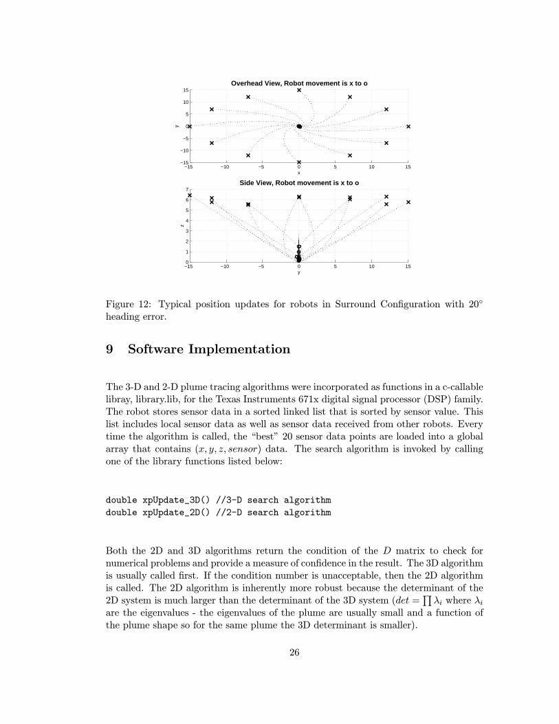
12 Typical position updates for robots in Surround Configuration with 20◦
heading error. . . . . . . . . . . . . . . . . . . . . . . . . . . . . . . . . . 26
6
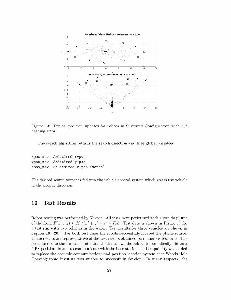
13 Typical position updates for robots in Surround Configuration with 30◦
heading error. . . . . . . . . . . . . . . . . . . . . . . . . . . . . . . . . . 27
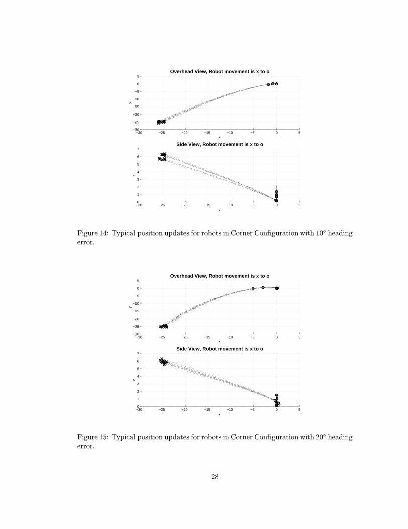
14 Typical position updates for robots in Corner Configuration with 10◦
heading error. . . . . . . . . . . . . . . . . . . . . . . . . . . . . . . . . 28
15 Typical position updates for robots in Corner Configuration with 20◦
heading error. . . . . . . . . . . . . . . . . . . . . . . . . . . . . . . . . 28
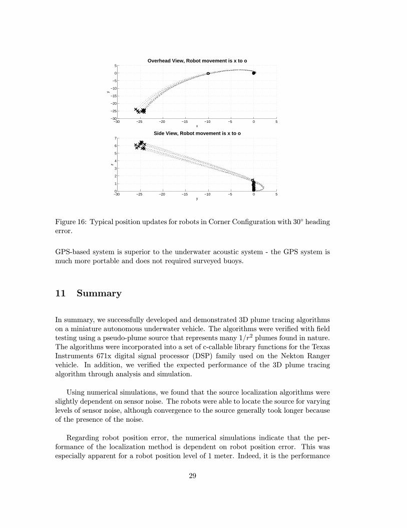
16 Typical position updates for robots in Corner Configuration with 30◦
heading error. . . . . . . . . . . . . . . . . . . . . . . . . . . . . . . . . 29
17 Test Results - Two Vehicles, Pseudo-Plume . . . . . . . . . . . . . . . . 30
18 Test Results - Pseudo-plume at depth of 1 meter . . . . . . . . . . . . . 31
19 Test Results - Pseudo-plume at depth of 3 meters . . . . . . . . . . . . . 32
20 Test Results - Pseudo-plume at depth of 5 meters . . . . . . . . . . . . . 33
7
1 Introduction
The goal of this research was to develop and demonstrate cooperative 3-D plume tracingalgorithms for miniature autonomous underwater vehicles. Applications for this tech-nology include Lost Asset and Survivor Location Systems (L-SALS) and Ship-in-PortPatrol and Protection (SP3). This research was a joint effort that included NektonResearch, LLC, Sandia National Laboratories, and Texas A&M University. NektonResearch developed the miniature autonomous underwater vehicles while Sandia devel-oped the 3-D plume tracing algorithms. The 3-D plume tracing algorithms are based ona 2-D plume tracing algorithm developed at Sandia for miniature mobile robots [1, 2].Johnny Hurtado at Texas A&M was involved with the original 2-D work while at Sandiaand helped with the 3-D algorithm development. Additional papers describing variousaspects of the algorithm have been submitted to several journals [3, 4, 5].
The 2-D plume tracing algorithm was originally designed for locating chemical,nuclear, or biological plumes using teams of miniature mobile robots. The algorithmswere successfully demonstrated in 1999 on teams of miniature mobile robots. The robotsemployed temperature sensors to seek out a temperature source generated with dry ice.A picture of the mobile robots appears in Figure 1. The goal of this project was todevelop a 3-D plume tracing algorithm based on the successful 2-D algorithm and thendemonstrate the 3-D algorithm on Nekton’s autonomous underwater vehicle. A pictureof Nekton’s autonomous underwater vehicle appears in Figure 2. The 3-D plume tracingalgorithms were successfully demonstrated in the Spring of 2003 using pseudo-plumesources. The pseudo-plume was a quadratic function F (x, y, z) ≈ K1/(x2+y2+z2+K2)that realistically models many 1/r2 plume sources.
The plume tracing algorithm is based on a quadratic estimation of the plume data.The robots then use this approximation to calculate a search direction. Each robot,or agent, has a table of plume data which consists of (x, y, z, f) data, where f is theplume amplitude sampled at (x, y, z). The table consists of data gathered by the robotas well as information received from other robots. Each agent may have a drasticallydifferent table of data depending on the type of communications (local or global) andthe location of the agent. There is no centralized control. Each robot independentlycalculates a search direction based on its table of sensor data.
A description of the 3-D plume tracing algorithm appears in the next section.
2 3-D Plume Tracing Algorithm
The central idea behind our cooperative localization method is to represent the truefunction with a local quadratic approximation. The control law for the ith robot is then
8
Figure 1: Miniature Robotic Vehicle
Figure 2: Nekton Research, LLC Miniature Autonomous Underwater Vehicle
9
based on the quadratic approximation.
In 3-dimensional space, a local quadratic approximation to the true function for theith robot reads
F (x, y, z) ≈ a0 + a1(x− xi) + a2(y − yi) + a3(z − zi)+ a4(x− xi)(y − yi) + a5(x− xi)(z − zi) + a6(y − yi)(z − zi)+1
2a7(x− xi)2 + 1
2a8(y − yi)2 + 1
2a9(z − zi)2.
In this equation, F (x, y, z) is the true function value as a function of (x, y, z), the triple(xi, yi, zi) represents the location of the ith robot, and aj are unknown coefficients thatdefine the quadratic approximation. Notice that the unknown coefficients aj appearlinearly in the quadratic approximation. This allows us to write an equation of theabove type for every neighboring robot and assemble the equations as a linear systemof equations of the form
Da = f
Here, D is the coefficient matrix, a is a vector of unknown coefficients, and f is thedata vector. More specifically, considering the jth neighboring robot, we have
Fj = F (xj , yj , zj) ≈ a0 + a1(xj − xi) + a2(yj − yi) + a3(zj − zi)+ a4(xj − xi)(yj − yi) + a5(xj − xi)(zj − zi) + a6(yj − yi)(zj − zi)+1
2a7(xj − xi)2 + 1
2a8(yj − yi)2 + 1
2a9(zj − zi)2.
So f becomes a column vector with entries {F1, F2, . . . , Fp}, where p is the number ofneighboring robots. The vector a is a column vector with entries {a0, a1, . . . , a9}. Andthe matrix D, dimensioned p × 10, has the relative robot positions as coefficients foreach of the p equations. That is, the jth row of the matrix D reads
D(j, :) = {1, (xj − xi), (yj − yi), (zj − zi), (xj − xi)(yj − yi),(xj − xi)(zj − zi), (yj − yi)(zj − zi), (xj − xi)2, (yj − yi)2, (zj − zi)2}.
Notice that because there are ten unknown coefficients we require at least ten neigh-boring robots, or ten valid sensor readings which may come from a single robot providedthe robot is able to utilize memory to store previous readings. The unknown coefficientsa are determined from the linear system of equations Da = f using the principle of leastsquares, which a robot’s micro controller can perform using QR factorization. This willbe discussed further subsequently.
Once the coefficients that define the quadratic model are computed, the update forthe ith robot is determined from equating the gradient of the function approximation
10
to zero. This leads to the position update equation
xi,new yi,new zi,newT= xi,old yi,old zi,old
T
+1
∆
a8a9 − a26 −a4a9 + a5a6 a4a6 − a5a8−a4a9 + a5a6 a7a9 − a25 −a7a6 + a4a5a4a6 − a5a8 −a7a6 + a4a5 a7a8 − a24
a1a2a3
,where
∆ = a7a8a9 − a7a26 − a24a9 + 2a4a5a6 − a25a8.
2.1 Determining the Unknown Coefficients for Ill-Conditioned Cases- Method I
In the previous section we arrived at the linear equation Da = f which must be solvedto determine the unknown coefficients a. The coefficients a define the local quadraticapproximation of the true function for the ith robot. A straightforward QR factorizationcan be used if the matrix D is well-conditioned, which will happen provided that thejth positions are sufficiently separated from the ith positions. Unfortunately, the matrixD can become ill-conditioned under innocent situations. For example, if the jth andith positions all occur in a constant z plane, then there is no z dependence in the dataand the matrix D will have a rank less than 10. This situation should be identifiedbefore the coefficients a are determined from Da = f . One method to identified thissituation is to perform a singular value decomposition on the matrix D. Indeed, theTotal Least Squares (TLS) method can be used to clearly identify which columns of Dare dependent.
The TLS method considers errors in a model (matrix D) as well as errors in thedata vector f . Traditional least squares (LS) only considers errors in the data vectorf . The basic TLS solution is given by
aTLS = (DTD − σ211I)−1DT f (1)
where σ11 is the 11th singular value of the augmented matrix [D; f ], which has dimensionp× 11. When D is rank-deficient, the nonzero entries of v11, which represents the 11th
right singular vector (or the 11th column of the right singular matrix) determine whichcolumns of D are dependent. These columns of D, and appropriate coefficients in a,can be discarded to produce a reduce model of the plume. For example, if the jth andith positions all occur in a constant z plane, then the 10th entry in v11 is nonzero, whichcorresponds to the z2 coefficient a9. Consequently, there is no quadratic z dependenceand columns [4,6,7,10] from D are removed, whereas columns [1,2,3,5,8,9] are retained.The reduced plume model is then a quadratic function of x and y only.
The reduced problem is written as Drar = f . This system of linear equations cannow be solved for the unknown coefficients ar using a QR factorization, or a singular
11
value decomposition (SVD) method, or a TLS method on a robot’s micro controller.The unknown coefficients ar are then used to compute the position update for the ith
robot.
2.2 Determining the Unknown Coefficients for Ill-Conditioned Cases- Method II
Another approach to handling ill-conditioned data is to check the condition of the Dmatrix when solving the matrix equation
Da = f (2)
where D is the coefficient matrix, a is the vector of unkown coefficients, and f is thedata vector. If the solution is calculated using a singular value decomposition, whichis the most robust numerical approach, the condition number C(D) is easily calculatedand defined by
C(D) =σ1σN
(3)
where σ1 is the largest singular value and σN is the smallest singular value. As thecondition number grows larger, the quality of the solution becomes questionable. Themost common numerical problem encountered during field testing was a lack of diver-sity in depth data for the 3-D case. Rather than looking at the depth data, the 3-Dalgorithm was modified to return the condition number as well as the search direction.By monitoring the condition number, the robot can switch to the 2-D algorithm if thedata does not have sufficent depth diversity. Another advantage of monitoring the con-dition number is that it will also catch other numerical problems (e.g. 3-D data in aplane). The condition number was also returned for the 2-D algorithm to catch poten-tial numerical problems in the 2-D case (e.g. data in a straight line). This approachwas implemented on the vehicles to handle numerical problems that can be encounteredwith typical sensor data.
The next section describes the light plume model.
3 Modeling of Light Data
In our work, we specifically considered underwater vehicles tasked with localizing alight source. We assumed that the light intensity varies from a source as the functionG(x, y, z) = k/R2, where R2 = (x−xs)2+(y−ys)2+(z−zs)2, k is some constant, and thetriple (xs, ys, zs) is the unknown source location. G(x, y, z) is the value that a vehiclesensor oriented directly toward the source would measure. Because the cooperative
12
localization method is based on a local quadratic approximation, we inverted the sensorreading F (x, y, z) = 1/G(x, y, z) and approximated the inverted reading F by a localquadratic approximation. The steps to determining a robot position update, as outlinedin the previous section, were carried out using the inverted sensor reading F .
4 Standard MATLAB Simulation Code
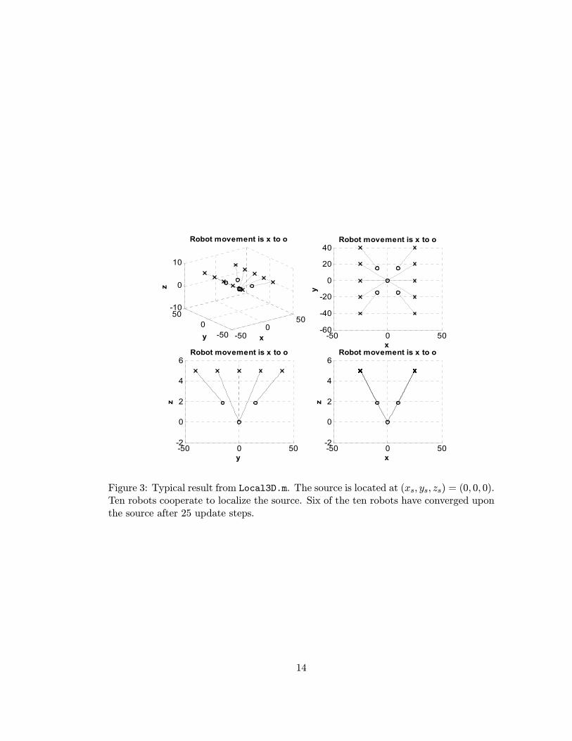
The 3-D localization algorithm was programmed in MATLAB. All MATLAB m-filesdeveloped for this project appear in Appendix A. The main simulation filename isLocal3D.m. Figure 3 shows a typical result from this simulation code. In this example,ten robots were placed in a volume. The source was located at the position (xs, ys, zs) =(0, 0, 0). The upper left plot shows the movement of the ten robots in 3-dimensionalspace; the upper right plot shows movement in the (x, y) plane; and the bottom plotsshow movement in the (y, z) and (x, z) planes. The plot shows that after 25 updatesteps, six of the ten robots have converged upon the source. The simulation was haltedafter 25 steps because, if not, then all ten robots would converge to the solution and theleading matrix D would become singular. In practice, this type of singularity conditionis avoided because two robots can not physically occupy the same location.
Simulation Comments:
1. The results are obtained by typing [x,y,z]=Local3D(’r2’,25) at the MATLABcommand prompt.
2. The output vectors of this function are the new x, y, z positions of all ten robots.3. The first input of this function ’r2’ is the filename that provides a robot’s sensorreading depending on its position.
4. The second input of this function 25 indicates the number of update steps to beperformed.
5. There are MATLAB files that support Local3D.m. These include getneighbors.m,getnewpos.m, and getupdate.m.
6. The files to run this simulation are found in the folder SimuA
5 Sensor Measurement Dependence on Vehicle Orienta-tion
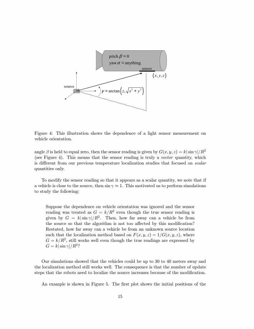
The measurement that a light sensor records is truly dependent on a vehicle’s orienta-tion. This was ignored in the previous discussion and simulation. If the vehicle pitch
13
-500
50
-500
50-10
0
10
x
Robot movement is x to o
y
z
-50 0 50-60
-40
-20
0
20
40Robot movement is x to o
x
y
-50 0 50-2
0
2
4
6Robot movement is x to o
y
z
-50 0 50-2
0
2
4
6Robot movement is x to o
x
z
Figure 3: Typical result from Local3D.m. The source is located at (xs, ys, zs) = (0, 0, 0).Ten robots cooperate to localize the source. Six of the ten robots have converged uponthe source after 25 update steps.
14
sensor
pitch 0yaw anything
βα
==
( ), ,x y z
( )2 2arctan ,z x yγ = +source
Figure 4: This illustration shows the dependence of a light sensor measurement onvehicle orientation.
angle β is held to equal zero, then the sensor reading is given by G(x, y, z) = k| sin γ|/R2(see Figure 4). This means that the sensor reading is truly a vector quantity, whichis different from our previous temperature localization studies that focused on scalarquantities only.
To modify the sensor reading so that it appears as a scalar quantity, we note that ifa vehicle is close to the source, then sin γ ≈ 1. This motivated us to perform simulationsto study the following:
Suppose the dependence on vehicle orientation was ignored and the sensorreading was treated as G = k/R2 even though the true sensor reading isgiven by G = k| sin γ|/R2. Then, how far away can a vehicle be fromthe source so that the algorithm is not too affected by this modification?Restated, how far away can a vehicle be from an unknown source locationsuch that the localization method based on F (x, y, z) = 1/G(x, y, z), whereG = k/R2, still works well even though the true readings are expressed byG = k| sin γ|/R2?
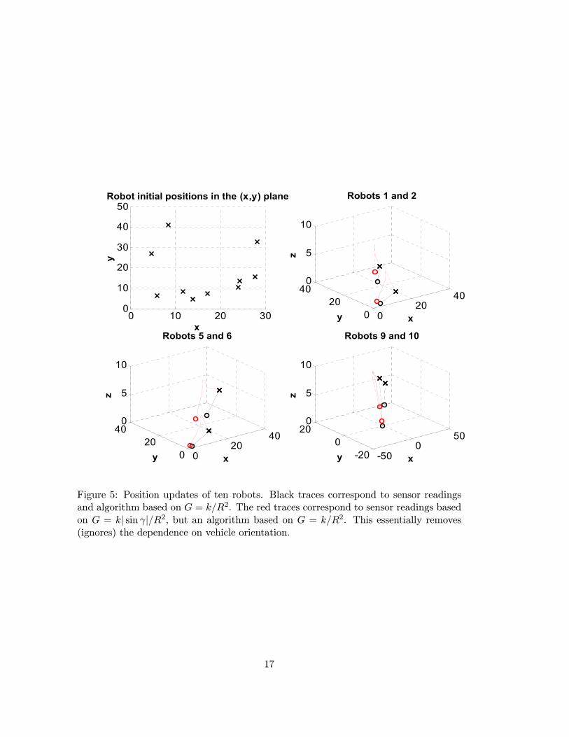
Our simulations showed that the vehicles could be up to 30 to 40 meters away andthe localization method still works well. The consequence is that the number of updatesteps that the robots need to localize the source increases because of the modification.
An example is shown in Figure 5. The first plot shows the initial positions of the
15
ten robots in the (x, y) plane. Some of the vehicles begin more than 30 meters awayfrom the source. In the other three plots, the black traces are the simulation resultsusing G = k/R2 as the sensor readings (i.e., not accounting for vehicle orientation)and using the algorithm based on this. The red traces are the simulation results usingG = k| sin γ|/R2 as the sensor readings (i.e., accounting for vehicle orientation) butusing the algorithm based onG = k/R2. The black traces show the vehicles immediatelyheading directly toward the unknown source location; The red traces do not show this.The red traces do show, however, that after the first few position updates, the vehiclesindeed begin heading toward the unknown source location. The black traces are shownfor 12 position updates, whereas the red traces are shown for 20 position updates. Aspreviously mentioned, the primary consequence of the modification is that the numberof update steps that the robots need to localize the source increases.
Simulation Comments:
1. The modified results, wherein the dependence on vehicle orientation is accountedfor in the sensor reading but ignored in the localization algorithm, are obtained bytyping [x,y,z]=Local3D(’r2depend’,20) at the MATLAB command prompt.Notice that the algorithm is the same (Local3D.m).
2. The input file, however, has changed to ’r2depend’. This input file accounts forthe sensor dependence on vehicle orientation.
3. The file ’r2depend.m’ is in the folder SimuA
6 Sensor Measurement Noise
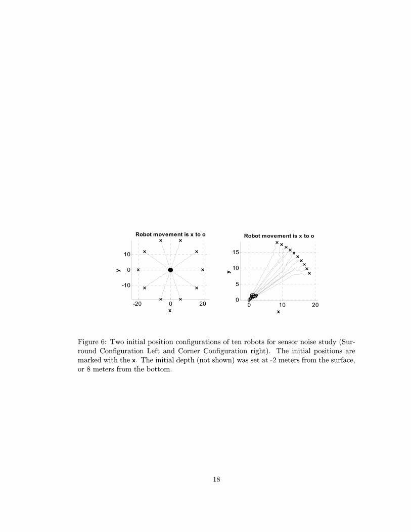
We performed numerical experiments to determine the influence of sensor noise on thelocalization method. We considered a pool measuring 50× 50× 10 meters and a teamof ten robots. We considered two different robot initial position configurations. In thefirst configuration, the robots essentially surround the unknown source location. Thisconfiguration is referred to as the Surround Configuration. In the second configuration,the robots begin in one corner of an area. This configuration is referred to as the CornerConfiguration. The two different initial position configurations are shown in Figure 6.
For the numerical simulations, the robots were given initial conditions like thoseabove but with an additional random initial position perturbation of up to one meter.The sensor noise level was set to equal a percent of the true value. As an example, fora 1 percent noise level, a sensor reading would fall between (100 ± 1)% of the actual(true) value. The cooperative algorithm was set to run for 50 position updates, with amaximum distance per update of 0.5 meters in the x, y, or z directions.
16
020
40
020
400
5
10
x
Robots 1 and 2
y
z
020
40
020
400
5
10
x
Robots 5 and 6
y
z
-500
50
-200
200
5
10
x
Robots 9 and 10
y
z
0 10 20 300
10
20
30
40
50Robot initial positions in the (x,y) plane
x
y
Figure 5: Position updates of ten robots. Black traces correspond to sensor readingsand algorithm based on G = k/R2. The red traces correspond to sensor readings basedon G = k| sin γ|/R2, but an algorithm based on G = k/R2. This essentially removes(ignores) the dependence on vehicle orientation.
17
-20 0 20
-10
0
10
Robot movement is x to o
x
y
0 10 200
5
10
15
Robot movement is x to o
x
y
Figure 6: Two initial position configurations of ten robots for sensor noise study (Sur-round Configuration Left and Corner Configuration right). The initial positions aremarked with the x. The initial depth (not shown) was set at -2 meters from the surface,or 8 meters from the bottom.
18
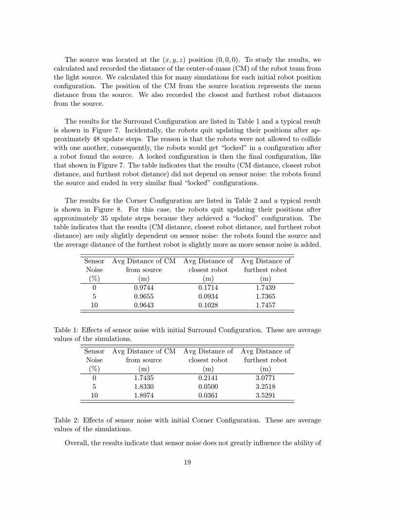
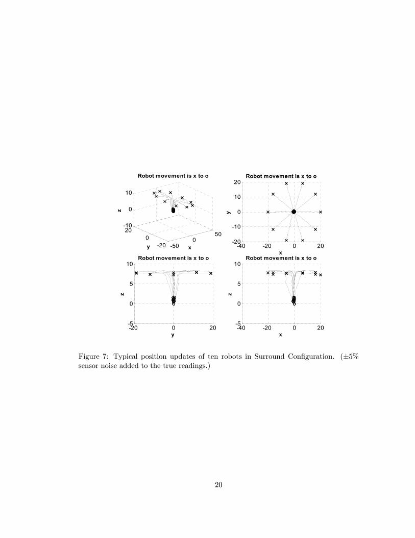
The source was located at the (x, y, z) position (0, 0, 0). To study the results, wecalculated and recorded the distance of the center-of-mass (CM) of the robot team fromthe light source. We calculated this for many simulations for each initial robot positionconfiguration. The position of the CM from the source location represents the meandistance from the source. We also recorded the closest and furthest robot distancesfrom the source.
The results for the Surround Configuration are listed in Table 1 and a typical resultis shown in Figure 7. Incidentally, the robots quit updating their positions after ap-proximately 48 update steps. The reason is that the robots were not allowed to collidewith one another, consequently, the robots would get “locked” in a configuration aftera robot found the source. A locked configuration is then the final configuration, likethat shown in Figure 7. The table indicates that the results (CM distance, closest robotdistance, and furthest robot distance) did not depend on sensor noise: the robots foundthe source and ended in very similar final “locked” configurations.
The results for the Corner Configuration are listed in Table 2 and a typical resultis shown in Figure 8. For this case, the robots quit updating their positions afterapproximately 35 update steps because they achieved a “locked” configuration. Thetable indicates that the results (CM distance, closest robot distance, and furthest robotdistance) are only slightly dependent on sensor noise: the robots found the source andthe average distance of the furthest robot is slightly more as more sensor noise is added.
Sensor Avg Distance of CM Avg Distance of Avg Distance ofNoise from source closest robot furthest robot(%) (m) (m) (m)
0 0.9744 0.1714 1.74395 0.9655 0.0934 1.736510 0.9643 0.1028 1.7457
Table 1: Effects of sensor noise with initial Surround Configuration. These are averagevalues of the simulations.
Sensor Avg Distance of CM Avg Distance of Avg Distance ofNoise from source closest robot furthest robot(%) (m) (m) (m)
0 1.7435 0.2141 3.07715 1.8330 0.0500 3.251810 1.8974 0.0361 3.5291
Table 2: Effects of sensor noise with initial Corner Configuration. These are averagevalues of the simulations.
Overall, the results indicate that sensor noise does not greatly influence the ability of
19
-500
50
-200
20-10
0
10
x
Robot movement is x to o
y
z
-40 -20 0 20-20
-10
0
10
20Robot movement is x to o
x
y
-20 0 20-5
0
5
10Robot movement is x to o
y
z
-40 -20 0 20-5
0
5
10Robot movement is x to o
x
z
Figure 7: Typical position updates of ten robots in Surround Configuration. (±5%sensor noise added to the true readings.)
20
010
20
-200
20-10
0
10
x
Robot movement is x to o
y
z
0 10 20-5
0
5
10
15
20Robot movement is x to o
x
y
-10 0 10 20-5
0
5
10Robot movement is x to o
y
z
0 10 20-5
0
5
10Robot movement is x to o
x
z
Figure 8: Typical position updates of ten robots in Corner Configuration. (±5% sensornoise added to the true readings.)
21
the localization method to find the source. The robots did take longer to converge to thesource when they started in the Surround Configuration (48 update steps) than whenthey started in the Corner Configuration (35 update steps). This can be witnessed bythe robot trajectories. In the initial Surround Configuration the robots first move in analmost horizontal plane before they begin to dive. In the initial Corner Configuration,the robots begin to dive as they move toward the source.
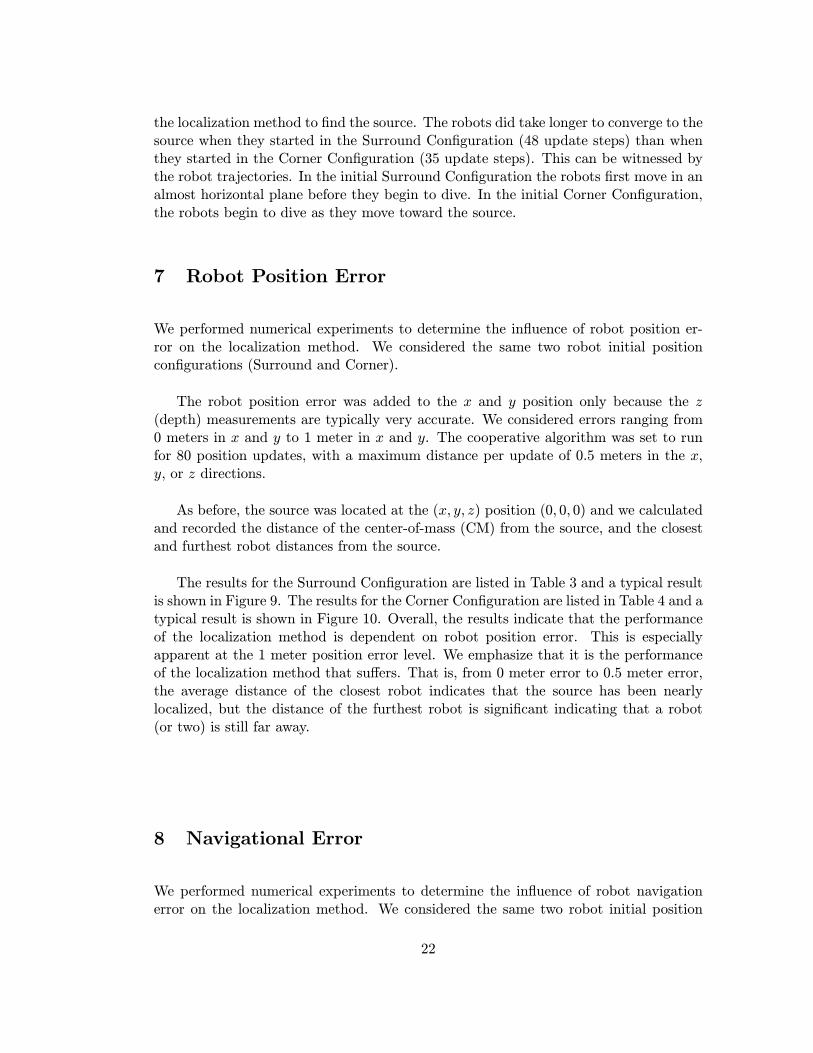
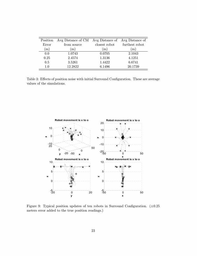
7 Robot Position Error
We performed numerical experiments to determine the influence of robot position er-ror on the localization method. We considered the same two robot initial positionconfigurations (Surround and Corner).
The robot position error was added to the x and y position only because the z(depth) measurements are typically very accurate. We considered errors ranging from0 meters in x and y to 1 meter in x and y. The cooperative algorithm was set to runfor 80 position updates, with a maximum distance per update of 0.5 meters in the x,y, or z directions.
As before, the source was located at the (x, y, z) position (0, 0, 0) and we calculatedand recorded the distance of the center-of-mass (CM) from the source, and the closestand furthest robot distances from the source.
The results for the Surround Configuration are listed in Table 3 and a typical resultis shown in Figure 9. The results for the Corner Configuration are listed in Table 4 and atypical result is shown in Figure 10. Overall, the results indicate that the performanceof the localization method is dependent on robot position error. This is especiallyapparent at the 1 meter position error level. We emphasize that it is the performanceof the localization method that suffers. That is, from 0 meter error to 0.5 meter error,the average distance of the closest robot indicates that the source has been nearlylocalized, but the distance of the furthest robot is significant indicating that a robot(or two) is still far away.
8 Navigational Error
We performed numerical experiments to determine the influence of robot navigationerror on the localization method. We considered the same two robot initial position
22
Position Avg Distance of CM Avg Distance of Avg Distance ofError from source closest robot furthest robot(m) (m) (m) (m)
0.0 1.0743 0.0705 2.10430.25 2.4574 1.3136 4.12510.5 3.5261 1.4422 6.67411.0 12.2822 6.1496 20.1739
Table 3: Effects of position noise with initial Surround Configuration. These are averagevalues of the simulations.
-500
50
-200
20-10
0
10
x
Robot movement is x to o
y
z
-50 0 50-20
-10
0
10
20Robot movement is x to o
x
y
-20 0 20-5
0
5
10Robot movement is x to o
y
z
-50 0 50-5
0
5
10Robot movement is x to o
x
z
Figure 9: Typical position updates of ten robots in Surround Configuration. (±0.25meters error added to the true position readings.)
23
Position Avg Distance of CM Avg Distance of Avg Distance ofError from source closest robot furthest robot(m) (m) (m) (m)
0.0 1.7470 0.0193 3.04230.25 2.0529 0.7228 4.07360.5 4.5930 1.8751 8.84561.0 13.3710 6.2784 25.3038
Table 4: Effects of position error with initial Corner Configuration. These are averagevalues of the simulations.
-200
20
-200
20-10
0
10
x
Robot movement is x to o
y
z
-10 0 10 20-5
0
5
10
15
20Robot movement is x to o
x
y
-10 0 10 20-5
0
5
10Robot movement is x to o
y
z
-10 0 10 20-5
0
5
10Robot movement is x to o
x
z
Figure 10: Typical position updates of ten robots in Corner Configuration. (±0.25meters error added to the true position readings.)
24
configurations (Surround and Corner).
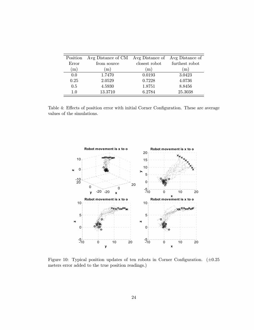
Heading error can be best visualized by considering a robot commanded to travel ina straight line. The error introduced will cause the robot to deviate from its intendedpath. The further the robot travels the greater the deviation. A larger error will meanthat the robot deviates faster from the path. We have assumed that the system canidentify the position of each robot exactly. Because of this assumption, the headingerror is harmless. Although the robot will not arrive at the exact location specified bythe algorithm update, the position sensors will be able to locate the new (deviated)position and calculate the next update using this information. The path a robot willtake to get to the source will be slightly longer than without navigation error.
Figures 11 through 13 show typical robot updates with heading errors ranging from10◦ to 30◦. The robots begin in a Surround Configuration. The heading error causethe robots to deviate from their intended path, but because the the robots can identifytheir true positions the robots are still able to locate the source.
−20 −15 −10 −5 0 5 10 15−20
−15
−10
−5
0
5
10
15Overhead View, Robot movement is x to o
x
y
−20 −15 −10 −5 0 5 10 150
1
2
3
4
5
6
7Side View, Robot movement is x to o
y
z
Figure 11: Typical position updates for robots in Surround Configuration with 10◦
heading error.
Figures 14 through 16 show typical robot updates with heading errors ranging from10◦ to 30◦ when the robots begin in a Corner Configuration. As with the SurroundConfiguration, the heading error cause the robots to deviate from their intended path,but because the the robots can identify their true positions the robots are still able tolocate the source.
25
−15 −10 −5 0 5 10 15−15
−10
−5
0
5
10
15Overhead View, Robot movement is x to o
xy
−15 −10 −5 0 5 10 150
1
2
3
4
5
6
7Side View, Robot movement is x to o
y
z
Figure 12: Typical position updates for robots in Surround Configuration with 20◦
heading error.
9 Software Implementation
The 3-D and 2-D plume tracing algorithms were incorporated as functions in a c-callablelibray, library.lib, for the Texas Instruments 671x digital signal processor (DSP) family.The robot stores sensor data in a sorted linked list that is sorted by sensor value. Thislist includes local sensor data as well as sensor data received from other robots. Everytime the algorithm is called, the “best” 20 sensor data points are loaded into a globalarray that contains (x, y, z, sensor) data. The search algorithm is invoked by callingone of the library functions listed below:
double xpUpdate_3D() //3-D search algorithm
double xpUpdate_2D() //2-D search algorithm
Both the 2D and 3D algorithms return the condition of the D matrix to check fornumerical problems and provide a measure of confidence in the result. The 3D algorithmis usually called first. If the condition number is unacceptable, then the 2D algorithmis called. The 2D algorithm is inherently more robust because the determinant of the2D system is much larger than the determinant of the 3D system (det = λi where λiare the eigenvalues - the eigenvalues of the plume are usually small and a function ofthe plume shape so for the same plume the 3D determinant is smaller).
26
−15 −10 −5 0 5 10 15 20−20
−10
0
10
20Overhead View, Robot movement is x to o
x
y
−20 −15 −10 −5 0 5 10 15 200
1
2
3
4
5
6
7Side View, Robot movement is x to o
y
z
Figure 13: Typical position updates for robots in Surround Configuration with 30◦
heading error.
The search algorithm returns the search direction via three global variables:
xpos_new //desired x-pos
ypos_new //desired y-pos
zpos_new // desired z-pos (depth)
The desired search vector is fed into the vehicle control system which steers the vehiclein the proper direction.
10 Test Results
Robot testing was performed by Nekton. All tests were performed with a pseudo plumeof the form F (x, y, z) ≈ K1/(x2 + y2 + z2 +K2). Test data is shown in Figure 17 fora test run with two vehicles in the water. Test results for three vehicles are shown inFigures 18 - 20. For both test cases the robots successfully located the plume source.These results are representative of the test results obtained on numerous test runs. Theperiodic rise to the surface is intentional - this allows the robots to periodically obtain aGPS position fix and to communicate with the base station. This capability was addedto replace the acoustic communications and position location system that Woods HoleOceanographic Institute was unable to successfully develop. In many respects, the
27
−30 −25 −20 −15 −10 −5 0 5−30
−25
−20
−15
−10
−5
0
5Overhead View, Robot movement is x to o
x
y
−30 −25 −20 −15 −10 −5 0 50
1
2
3
4
5
6
7Side View, Robot movement is x to o
y
z
Figure 14: Typical position updates for robots in Corner Configuration with 10◦ headingerror.
−30 −25 −20 −15 −10 −5 0 5−30
−25
−20
−15
−10
−5
0
5Overhead View, Robot movement is x to o
x
y
−30 −25 −20 −15 −10 −5 0 50
1
2
3
4
5
6
7Side View, Robot movement is x to o
y
z
Figure 15: Typical position updates for robots in Corner Configuration with 20◦ headingerror.
28
−30 −25 −20 −15 −10 −5 0 5−30
−25
−20
−15
−10
−5
0
5Overhead View, Robot movement is x to o
x
y
−30 −25 −20 −15 −10 −5 0 50
1
2
3
4
5
6
7Side View, Robot movement is x to o
y
z
Figure 16: Typical position updates for robots in Corner Configuration with 30◦ headingerror.
GPS-based system is superior to the underwater acoustic system - the GPS system ismuch more portable and does not required surveyed buoys.
11 Summary
In summary, we successfully developed and demonstrated 3D plume tracing algorithmson a miniature autonomous underwater vehicle. The algorithms were verified with fieldtesting using a pseudo-plume source that represents many 1/r2 plumes found in nature.The algorithms were incorporated into a set of c-callable library functions for the TexasInstruments 671x digital signal processor (DSP) family used on the Nekton Rangervehicle. In addition, we verified the expected performance of the 3D plume tracingalgorithm through analysis and simulation.
Using numerical simulations, we found that the source localization algorithms wereslightly dependent on sensor noise. The robots were able to locate the source for varyinglevels of sensor noise, although convergence to the source generally took longer becauseof the presence of the noise.
Regarding robot position error, the numerical simulations indicate that the per-formance of the localization method is dependent on robot position error. This wasespecially apparent for a robot position level of 1 meter. Indeed, it is the performance
29
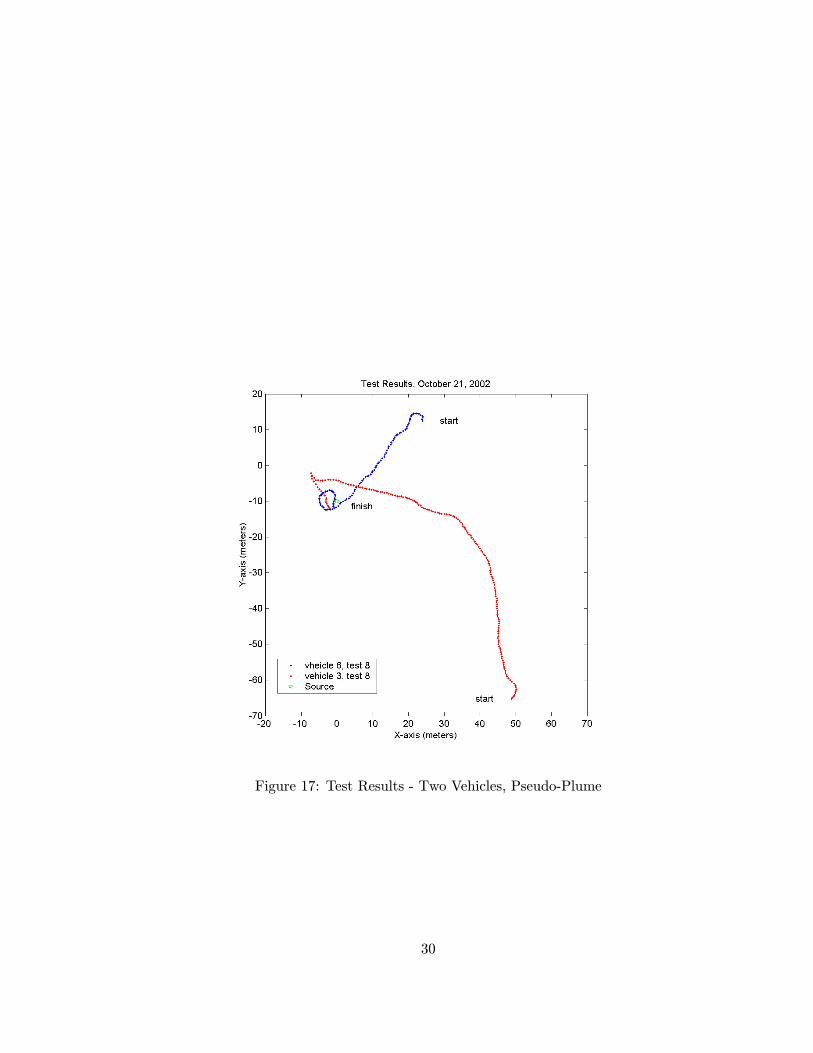
Figure 17: Test Results - Two Vehicles, Pseudo-Plume
30
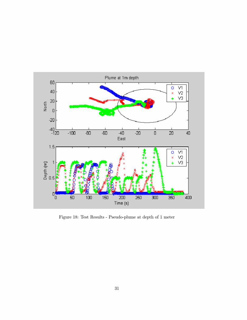
Figure 18: Test Results - Pseudo-plume at depth of 1 meter
31
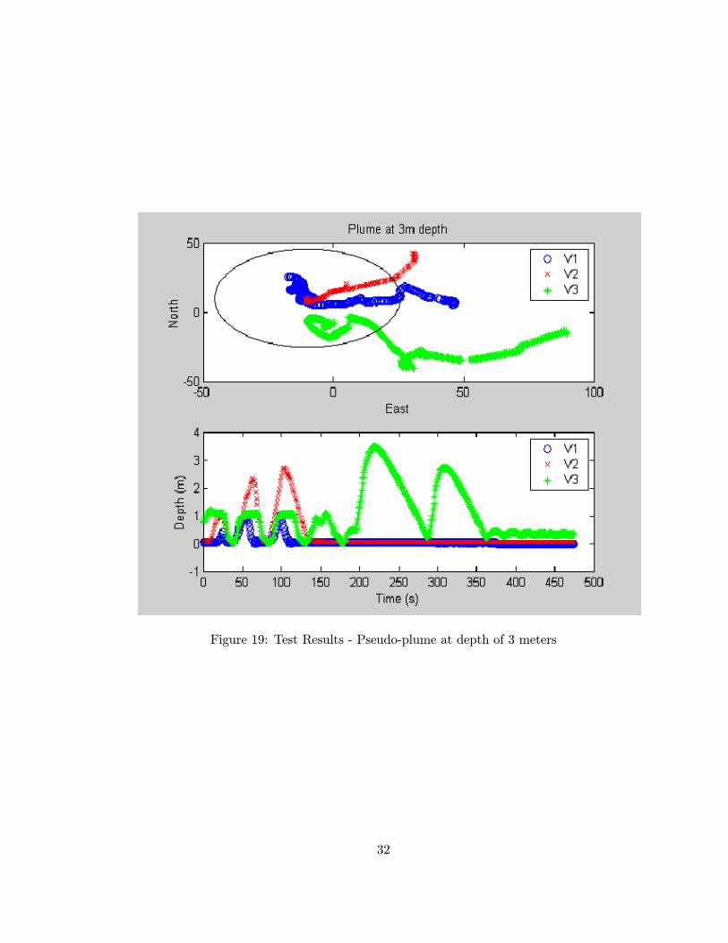
Figure 19: Test Results - Pseudo-plume at depth of 3 meters
32
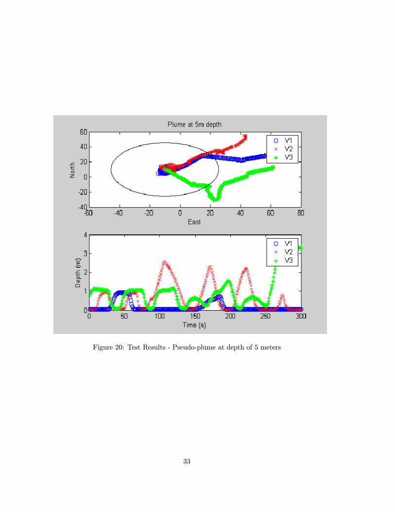
Figure 20: Test Results - Pseudo-plume at depth of 5 meters
33
of the localization method that suffers, in that the average distance of the closest robotfor a typical simulation indicates that the source has been nearly localized, but thedistance of the furthest robot is significant indicating that a robot (or two) is still faraway.
From numerical simulation, the algorithm was found to be robust with regard tonavigation or heading error. Heading error will cause the robot to deviate from itsintended path. As long as a robot could correctly identify its position, however, thistype of error was not found a problem. The robots were able to localize the sourcealthough the eventual path was found to deviate from the original intended path.
12 Acknowledgments
Many people were instrumental in making this project a success. Johnny Hurtadowith assistance from Elizabeth Savage developed the 3-D algorithm and performed thesimulation studies. Steven Eskridge coded the algorithm for the 671x DSP. Ray Byrnemade minor modifications to the algorithm (applied different numerical techniques),completed the DSP coding, and served as project leader and principal investigator.Heather Pinnix and Bryan Schulz at Nekton integrated the Sandia code with the Nektonvehicle and performed the field testing. The Nekton team also included: Brett Hobson,Mathieu Kemp, Jim Meyer, Ryan Moody, Mathew St. Clair, Jeff Bourn, GordonCaudle, Harriet Crisp, Rick Vosburgh, and Jason Janet. Dr. Elana Ethridge served asthe DARPA program manager for this effort.
References
[1] J. E. Hurtado, R. H. Byrne, S. E. Eskridge, and J. J. Harrington, “Miniature mobilerobots for plume tracking and source localization research.” Workshop on MobileMicro-Robots, 2000 IEEE International Conference on Robotics and Automation,April 28, 2000.
[2] R. H. Byrne, D. R. Adkins, S. E. Eskridge, J. J. Harrington, E. J. Heller, andJ. E. Hurtado, “Miniature mobile robots for plume tracking and source localizationresearch,” Journal of Micromechatronics, vol. 1, no. 3, pp. 253—261, 2002.
[3] J. E. Hurtado and R. D. Robinett, “Convergence of newton’s method via lyapunovanalysis.” Submitted to the Journal of Guidance, Control, and Dynamics (October2002).
[4] J. E. Hurtado and R. D. Robinett, “Control design, stability and performance forrobotic collectives.” Submitted to the Journal of Intelligent and Robotic Systems:Theory and Applications (October 2002).
34

[5] J. E. Hurtado, R. D. Robinett, C. R. Dohrmann, and S. Y. Goldsmith, “Decentral-ized control for a swarm of vehicles performing source localization.” Submitted tothe Journal of Intelligent and Robotic Systems: Theory and Applications (October2002).
35
A MATLAB M-FILES
A.1 batchsimu.m
N=80;
for indx=1:5,
[x,y,z]=local3DSN(’r2depend’,N);
R=x(N+1,:).^2+y(N+1,:).^2+z(N+1,:).^2;
R=sqrt(R);
CM(indx) = mean(R);
Sm(indx) = min(R);
Lg(indx) = max(R);
[CM;Sm;Lg]
end
A.2 getneighbors.m
function [iflag,ii]=getneighbors(i,xa,ya,za,scrmin,scrmax)
% find the neighbors near robot i
iflag=1;
xd=xa-xa(i); yd=ya-ya(i); zd=za-za(i);
r=sqrt(xd.*xd + yd.*yd + zd.*zd);
rcurr=scrmin;
ii=find(r<scrmin);
if length(ii)<10
iflag=0; rcurr=scrmin;
while iflag==0,
rcurr=1.5*rcurr;
ii=find(r<rcurr);
if length(ii)>=10
iflag=1;
end
if rcurr>scrmax,
iflag=2;
end
end
end
A.3 getnewpos.m
function [delx,dely,delz]=getnewpos(i,p,dxmax,dymax,dzmax,xa,ya,za,nxy)
dx=p(1); dy=p(2); dz=p(3);
36
sf=max([abs(dx)/dxmax(i),abs(dy)/dymax(i),abs(dz)/dzmax(i)]);
alpha=min(1,1/sf);
mx=1;
delx=alpha*dx;
dely=alpha*dy;
delz=alpha*dz;
% return % turn off the "collision check"
% collision avoidance to remove simulation singularity
mx=1;
tooclose=1;
while tooclose==1;
tooclose=0;
delxnew=mx*alpha*dx;
delynew=mx*alpha*dy;
delznew=mx*alpha*dz;
xnew=xa(i)+delxnew;
ynew=ya(i)+delynew;
znew=za(i)+delznew;
xd=xnew-xa; yd=ynew-ya; zd=znew-za;
r=sqrt(xd.*xd + yd.*yd + zd.*zd);
ro=.5;
% ro=.5;
for L=1:nxy,
if L~=i
if r(L)<ro,
tooclose=1;
mx=mx-.1;;
end
end
end
end
delx=delxnew;
dely=delynew;
delz=delznew;
A.4 getupdate.m
function p=getupdate(ii,i,xa,ya,za,b,nxy)
% flag==1, solve the LS problem
% flag==2, solve the TLS problem
% xc=(xa(ii) + rangenoise(ii)’)’;
xc=(xa(ii))’;
yc=(ya(ii))’;
zc=(za(ii))’;
xcnoise=xc;
37
ycnoise=yc;
zcnoise=zc;
xcn=xcnoise-xa(i); ycn=ycnoise-ya(i); zcn=zcnoise-za(i);
A=zeros(length(ii),10);
A=[ones(length(ii),1) xcn ycn zcn xcn.*xcn/2 ycn.*ycn/2 zcn.*zcn/2
xcn.*ycn xcn.*zcn ycn.*zcn];
bpart=zeros(length(ii),1);
bpart(:,1)=b(ii(:),1);
a=A\bpart(:,1);
tol=.01;
H=[a(5) a(8) a(9);
a(8) a(6) a(10);
a(9) a(10) a(7)];
if(min(eig(H)))<tol,
[v,d]=eig(H);
H=v*abs(d)*inv(v);
end
bp=-[a(2);a(3);a(4)];
p=H\bp;
A.5 input r2.m
% input file
nx=2; ny=5; nz=1; % total number of bugs
nxy=nx*ny*nz;
% close
boun=[-20,20,-20,20,0,10];
bounp=boun;
% far
%boun=[-50,50,-50,50,0,10];
%bounp=boun;
%boun=1.3*[28,22,28,22,1,9];
%bounp=1.3*[-30,30,-30,30,0,10];
aleft=boun(1); aright=boun(2); % left/right boundaries
bleft=boun(3); bright=boun(4); % left/right boundaries
cleft=boun(5); cright=boun(6); % left/right boundaries
apl=bounp(1); apr=bounp(2); % left/right boundaries for plotting
bpl=bounp(3); bpr=bounp(4);
cpl=bounp(5); cpr=bounp(6);
dx=(aright-aleft)/nx; % partition up the grid
dy=(bright-bleft)/ny;
38
dz=(cright-cleft)/nz;
dxmax=1; dymax=1; dzmax=1; % max allowable dx,dy step for optimization
dxmax=dxmax*ones(1,nxy);
dymax=dymax*ones(1,nxy);
dzmax=dzmax*ones(1,nxy);
sensornoise=0 * 1/500*(rand(nxy,1)-0.5);
rangenoise= 0 * 1/10*(rand(nxy,1)-0.5);
percentSN = 0;
scrmin = 100;
scrmax = 100;
A.6 input r2depend.m
% input file
nx=2; ny=5; nz=1; % total number of bugs
nxy=nx*ny*nz;
% close
boun=[-20,20,-20,20,0,10];
bounp=boun;
% far
%boun=[-50,50,-50,50,0,10];
%bounp=boun;
%boun=1.3*[28,22,28,22,1,9];
%bounp=1.3*[-30,30,-30,30,0,10];
aleft=boun(1); aright=boun(2); % left/right boundaries
bleft=boun(3); bright=boun(4); % left/right boundaries
cleft=boun(5); cright=boun(6); % left/right boundaries
apl=bounp(1); apr=bounp(2); % left/right boundaries for plotting
bpl=bounp(3); bpr=bounp(4);
cpl=bounp(5); cpr=bounp(6);
dx=(aright-aleft)/nx; % partition up the grid
dy=(bright-bleft)/ny;
dz=(cright-cleft)/nz;
dxmax=.5; dymax=.5; dzmax=.5; % max allowable dx,dy step for optimization
dxmax=dxmax*ones(1,nxy);
dymax=dymax*ones(1,nxy);
dzmax=dzmax*ones(1,nxy);
39
sensornoise=0 * 1/500*(rand(nxy,1)-0.5); % not used but keep at zero
rangenoise= 0 * 1/10*(rand(nxy,1)-0.5); % not used but keep at zero
percentSN = 0; % sensor noise percent
percentPN = 1; % position noise in meters
scrmin = 100;
scrmax = 100;
A.7 local3D.m
function [xLS,yLS,zLS]=dscc3D(fcn,nstep)
% function [xLS,yLS,xTLS,yTLS]=dscc(fcn,cflag,nstep,xa,ya,za)
%
% fcn: character string of function (must also have input fcn name)
% nstep: number of steps (updates) to perform
% xa, ya: if cflag=’onn’, then starting positions for continuation
% if cflag=’off’, then this will be reset
%
%
%--------------------------------------------------------------------------
% 1. Finds which bugs are close.
% 2. Fixes Hessian if not positive definite.
% 3. Robot Avoidance: Takes step length of alpha along search direction.
% If too close to another robot then backs off until not too close.
% 4. Each updates when ready. Do not wait.
eval([’input_’ fcn ]);
cflag=’off’;
if cflag==’off’,
x=aleft+dx/2:dx:aright-dx/2;
y=bleft+dy/2:dy:bright-dy/2;
z=cleft+dz/2:dz:cright-dz/2;
xa=zeros(1,nxy);
ya=zeros(1,nxy);
za=zeros(1,nxy);
for i=1:ny
ibeg=(i-1)*nx+1;
iend=i*nx;
xa(ibeg:iend)=x;
ya(ibeg:iend)=y(i)*ones(1,nx);
za(ibeg:iend)=z(1)*ones(1,nx);
end
sp=1/2*.0001;
xa=xa+2*sp*dx*(rand(1,nxy)-0.5);
ya=ya+2*sp*dy*(rand(1,nxy)-0.5);
40
za=za+2*sp*dz*(rand(1,nxy)-0.5);
end
% specified initial positions ... useful for comparison purposes.
xa = [34.3148 56.2963 11.8889 16.9021 27.8895 55.6815
48.5589 9.5222 23.1921 47.8658]*.5;
ya = [14.4320 65.1551 12.4608 81.5887 9.3024 30.9941
26.8817 53.6451 16.3278 21.0988]*.5;
za = [0.6828 1.2523 1.6615 9.1142 1.3626 6.1700
2.6898 2.2066 7.1290 5.4900];
xLS(1,:)=xa;
yLS(1,:)=ya;
zLS(1,:)=za;
figure(1), clf
subplot(221), plot3(xa,ya,za,’kx’,’markersize’,10,’linewidth’,2); hold on,
subplot(222), plot3(xa,ya,za,’kx’,’markersize’,10,’linewidth’,2); hold on,
subplot(223), plot3(xa,ya,za,’kx’,’markersize’,10,’linewidth’,2); hold on,
subplot(224), plot3(xa,ya,za,’kx’,’markersize’,10,’linewidth’,2); hold on,
for k=1:nstep
eval([’bLS=’ fcn ’(xa,ya,za);’]);
for i=1:nxy
% eval([’bLS=’ fcn ’(xa,ya,za);’]);
[iflagLS,iiLS]=getneighbors(i,xa,ya,za,scrmin,scrmax);
if iflagLS==1,
pLS=getupdate(iiLS,i,xa,ya,za,bLS,nxy);
[delxLS(i),delyLS(i),delzLS(i)]=getnewpos(i,pLS,dxmax,dymax,dzmax,xa,ya,za,nxy);
elseif iflagLS==2,
delxLS(i)=0; delyLS(i)=0; delzLS(i)=0;
end
% update when ready
% xa(i)=xa(i)+delxLS(i);
% ya(i)=ya(i)+delyLS(i);
% za(i)=za(i)+delzLS(i);
% if za(i)<0, za(i)=0; end
end
% everyone update at once
for i=1:nxy
xa(i)=xa(i)+delxLS(i);
ya(i)=ya(i)+delyLS(i);
za(i)=za(i)+delzLS(i);
end
41
xLS(k+1,:)=xa;
yLS(k+1,:)=ya;
zLS(k+1,:)=za;
end
figure(1),
subplot(221),
plot3(xa,ya,za,’ko’,’markersize’,6,’linewidth’,2);
%plot(xb,yb,’ro’,’markersize’,6,’linewidth’,2);
for i=1:nxy, plot3(xLS(:,i),yLS(:,i),zLS(:,i),’k:’,’linewidth’,1); end
%for i=1:nxy, plot(xTLS(:,i),yTLS(:,i),’r’,’linewidth’,1); end
xlabel(’x’,’fontsize’,14,’fontweight’,’bold’),
ylabel(’y’,’fontsize’,14,’fontweight’,’bold’),
title(’Robot movement is x to o’,’fontsize’,14,’fontweight’,’bold’);
zlabel(’z’,’fontsize’,14,’fontweight’,’bold’),
h=gca;
set(h,’fontsize’,14);
grid on
hold off
subplot(222),
plot3(xa,ya,za,’ko’,’markersize’,6,’linewidth’,2);
for i=1:nxy, plot3(xLS(:,i),yLS(:,i),zLS(:,i),’k:’,’linewidth’,1); end
xlabel(’x’,’fontsize’,14,’fontweight’,’bold’),
ylabel(’y’,’fontsize’,14,’fontweight’,’bold’),
title(’Robot movement is x to o’,’fontsize’,14,’fontweight’,’bold’);
zlabel(’z’,’fontsize’,14,’fontweight’,’bold’),
h=gca;
set(h,’fontsize’,14);
grid on
hold off
view(2)
subplot(223),
plot3(xa,ya,za,’ko’,’markersize’,6,’linewidth’,2);
for i=1:nxy, plot3(xLS(:,i),yLS(:,i),zLS(:,i),’k:’,’linewidth’,1); end
xlabel(’x’,’fontsize’,14,’fontweight’,’bold’),
ylabel(’y’,’fontsize’,14,’fontweight’,’bold’),
title(’Robot movement is x to o’,’fontsize’,14,’fontweight’,’bold’);
zlabel(’z’,’fontsize’,14,’fontweight’,’bold’),
h=gca;
set(h,’fontsize’,14);
grid on
hold off
view(90,0)
subplot(224),
plot3(xa,ya,za,’ko’,’markersize’,6,’linewidth’,2);
for i=1:nxy, plot3(xLS(:,i),yLS(:,i),zLS(:,i),’k:’,’linewidth’,1); end
xlabel(’x’,’fontsize’,14,’fontweight’,’bold’),
42
ylabel(’y’,’fontsize’,14,’fontweight’,’bold’),
title(’Robot movement is x to o’,’fontsize’,14,’fontweight’,’bold’);
zlabel(’z’,’fontsize’,14,’fontweight’,’bold’),
h=gca;
set(h,’fontsize’,14);
grid on
hold off
view(0,0)
% XTRAS
%xcm=zeros(nstep+1,1); ycm=zeros(nstep+1,1);
%xcm(1,1)=sum(xa)/nxy; ycm(1,1)=sum(ya)/nxy;
%plot(xa,ya,’bx’,xcm(1,1),ycm(1,1),’mx’); hold on,
%plot(xcm(:,1),ycm(:,1),’m’)
%plot(xcm(nstep+1,1),ycm(nstep+1,1),’mo’)
A.8 Local3DSN.m
function [xLS,yLS,zLS]=dscc3D(fcn,nstep)
% function [xLS,yLS,xTLS,yTLS]=dscc(fcn,cflag,nstep,xa,ya,za)
%
% fcn: character string of function (must also have input fcn name)
% nstep: number of steps (updates) to perform
% xa, ya: if cflag=’onn’, then starting positions for continuation
% if cflag=’off’, then this will be reset
%
%
%--------------------------------------------------------------------------
% 1. Finds which bugs are close.
% 2. Fixes Hessian if not positive definite.
% 3. Robot Avoidance: Takes step length of alpha along search direction.
% If too close to another robot then backs off until not too close.
% 4. Each updates when ready. Do not wait.
eval([’input_’ fcn ]);
cflag=’off’;
if cflag==’off’,
x=aleft+dx/2:dx:aright-dx/2;
y=bleft+dy/2:dy:bright-dy/2;
z=cleft+dz/2:dz:cright-dz/2;
xa=zeros(1,nxy);
ya=zeros(1,nxy);
za=zeros(1,nxy);
for i=1:ny
ibeg=(i-1)*nx+1;
43
iend=i*nx;
xa(ibeg:iend)=x;
ya(ibeg:iend)=y(i)*ones(1,nx);
za(ibeg:iend)=z(1)*ones(1,nx);
end
sp=1/2*.0001;
xa=xa+2*sp*dx*(rand(1,nxy)-0.5);
ya=ya+2*sp*dy*(rand(1,nxy)-0.5);
za=za+2*sp*dz*(rand(1,nxy)-0.5);
end
% specified initial positions ... useful for comparison purposes.
%xa = [34.3148 56.2963 11.8889 16.9021 27.8895
% 55.6815 48.5589 9.5222 23.1921 47.8658]*.5;
%ya = [14.4320 65.1551 12.4608 81.5887 9.3024
% 30.9941 26.8817 53.6451 16.3278 21.0988]*.5;
%za = [0.6828 1.2523 1.6615 9.1142 1.3626
% 6.1700 2.6898 2.2066 7.1290 5.4900];
percentRN = .1;
R = 20*(1 + percentRN/100 * 2*(rand(1,nxy)-0.5));
theta = linspace(0,324,10)*pi/180; % surround
%theta = linspace(25,65,10)*pi/180; % corner arc
xa = R.*cos(theta);
ya = R.*sin(theta);
za = 8 * (1 + 10/100 * (rand(1,nxy)-1));
xLS(1,:)=xa;
yLS(1,:)=ya;
zLS(1,:)=za;
figure(1), clf
subplot(221), plot3(xa,ya,za,’kx’,’markersize’,10,’linewidth’,2); hold on,
subplot(222), plot3(xa,ya,za,’kx’,’markersize’,10,’linewidth’,2); hold on,
subplot(223), plot3(xa,ya,za,’kx’,’markersize’,10,’linewidth’,2); hold on,
subplot(224), plot3(xa,ya,za,’kx’,’markersize’,10,’linewidth’,2); hold on,
for k=1:nstep
% for update at once
% eval([’bLS=’ fcn ’(xa,ya,za);’]);
% bLS = bLS*(1 + percentSN/100 * 2*(rand(1,nxy)-0.5));
for i=1:nxy
% for update when ready
eval([’bLS=’ fcn ’(xa,ya,za);’]);
bLS = bLS*(1 + percentSN/100 * 2*(rand(1,nxy)-0.5));
xa = xa + percentPN * 2*(rand(1,nxy)-0.5);
ya = ya + percentPN * 2*(rand(1,nxy)-0.5);
[iflagLS,iiLS]=getneighbors(i,xa,ya,za,scrmin,scrmax);
44
if iflagLS==1,
pLS=getupdate(iiLS,i,xa,ya,za,bLS,nxy);
[delxLS(i),delyLS(i),delzLS(i)]=getnewpos(i,pLS,dxmax,dymax,dzmax,xa,ya,za,nxy);
elseif iflagLS==2,
delxLS(i)=0; delyLS(i)=0; delzLS(i)=0;
end
% update when ready
xa(i)=xa(i)+delxLS(i);
ya(i)=ya(i)+delyLS(i);
za(i)=za(i)+delzLS(i);
% if za(i)<0, za(i)=0; end
end
% everyone update at once
% for i=1:nxy
% xa(i)=xa(i)+delxLS(i);
% ya(i)=ya(i)+delyLS(i);
% za(i)=za(i)+delzLS(i);
% end
xLS(k+1,:)=xa;
yLS(k+1,:)=ya;
zLS(k+1,:)=za;
end
figure(1),
subplot(221),
plot3(xa,ya,za,’ko’,’markersize’,6,’linewidth’,2);
%plot(xb,yb,’ro’,’markersize’,6,’linewidth’,2);
for i=1:nxy, plot3(xLS(:,i),yLS(:,i),zLS(:,i),’k:’,’linewidth’,1); end
%for i=1:nxy, plot(xTLS(:,i),yTLS(:,i),’r’,’linewidth’,1); end
xlabel(’x’,’fontsize’,14,’fontweight’,’bold’),
ylabel(’y’,’fontsize’,14,’fontweight’,’bold’),
title(’Robot movement is x to o’,’fontsize’,14,’fontweight’,’bold’);
zlabel(’z’,’fontsize’,14,’fontweight’,’bold’),
h=gca;
set(h,’fontsize’,14);
grid on
hold off
subplot(222),
plot3(xa,ya,za,’ko’,’markersize’,6,’linewidth’,2);
for i=1:nxy, plot3(xLS(:,i),yLS(:,i),zLS(:,i),’k:’,’linewidth’,1); end
xlabel(’x’,’fontsize’,14,’fontweight’,’bold’),
ylabel(’y’,’fontsize’,14,’fontweight’,’bold’),
title(’Robot movement is x to o’,’fontsize’,14,’fontweight’,’bold’);
zlabel(’z’,’fontsize’,14,’fontweight’,’bold’),
h=gca;
45
set(h,’fontsize’,14);
grid on
hold off
view(2)
subplot(223),
plot3(xa,ya,za,’ko’,’markersize’,6,’linewidth’,2);
for i=1:nxy, plot3(xLS(:,i),yLS(:,i),zLS(:,i),’k:’,’linewidth’,1); end
xlabel(’x’,’fontsize’,14,’fontweight’,’bold’),
ylabel(’y’,’fontsize’,14,’fontweight’,’bold’),
title(’Robot movement is x to o’,’fontsize’,14,’fontweight’,’bold’);
zlabel(’z’,’fontsize’,14,’fontweight’,’bold’),
h=gca;
set(h,’fontsize’,14);
grid on
hold off
view(90,0)
subplot(224),
plot3(xa,ya,za,’ko’,’markersize’,6,’linewidth’,2);
for i=1:nxy, plot3(xLS(:,i),yLS(:,i),zLS(:,i),’k:’,’linewidth’,1); end
xlabel(’x’,’fontsize’,14,’fontweight’,’bold’),
ylabel(’y’,’fontsize’,14,’fontweight’,’bold’),
title(’Robot movement is x to o’,’fontsize’,14,’fontweight’,’bold’);
zlabel(’z’,’fontsize’,14,’fontweight’,’bold’),
h=gca;
set(h,’fontsize’,14);
grid on
hold off
view(0,0)
% XTRAS
%xcm=zeros(nstep+1,1); ycm=zeros(nstep+1,1);
%xcm(1,1)=sum(xa)/nxy; ycm(1,1)=sum(ya)/nxy;
%plot(xa,ya,’bx’,xcm(1,1),ycm(1,1),’mx’); hold on,
%plot(xcm(:,1),ycm(:,1),’m’)
%plot(xcm(nstep+1,1),ycm(nstep+1,1),’mo’)
A.9 plotcompare.m
% a plot function for comparison
figure(2),
N=1:10;
subplot(221), plot3(xLS(1,N),yLS(1,N),zLS(1,N),’kx’,’markersize’,10,’linewidth’,2); hold on,
xlabel(’x’,’fontsize’,14,’fontweight’,’bold’), ylabel(’y’,’fontsize’,14,’fontweight’,’bold’),
title(’Robot initial positions in the (x,y) plane’,’fontsize’,14,’fontweight’,’bold’);
46
zlabel(’z’,’fontsize’,14,’fontweight’,’bold’),
h=gca;
set(h,’fontsize’,14);
view(2),
grid on
hold off
N=1:2;
subplot(222), plot3(xLS(1,N),yLS(1,N),zLS(1,N),’kx’,’markersize’,10,’linewidth’,2); hold on,
subplot(222), plot3(xLSg(1,N),yLSg(1,N),zLSg(1,N),’kx’,’markersize’,10,’linewidth’,2);
subplot(222), plot3(xLS(13,N),yLS(13,N),zLS(13,N),’ko’,’markersize’,6,’linewidth’,2); hold on,
subplot(222), plot3(xLSg(21,N),yLSg(21,N),zLSg(21,N),’ro’,’markersize’,6,’linewidth’,2);
for i=N, plot3(xLS(:,i),yLS(:,i),zLS(:,i),’k:’,’linewidth’,1); end
for i=N, plot3(xLSg(:,i),yLSg(:,i),zLSg(:,i),’r:’,’linewidth’,1); end
xlabel(’x’,’fontsize’,14,’fontweight’,’bold’), ylabel(’y’,’fontsize’,14,’fontweight’,’bold’),
title(’Robots 1 and 2’,’fontsize’,14,’fontweight’,’bold’);
zlabel(’z’,’fontsize’,14,’fontweight’,’bold’),
h=gca;
set(h,’fontsize’,14);
grid on
hold off
N=5:6;
subplot(223), plot3(xLS(1,N),yLS(1,N),zLS(1,N),’kx’,’markersize’,10,’linewidth’,2); hold on,
subplot(223), plot3(xLSg(1,N),yLSg(1,N),zLSg(1,N),’kx’,’markersize’,10,’linewidth’,2);
subplot(223), plot3(xLS(13,N),yLS(13,N),zLS(13,N),’ko’,’markersize’,6,’linewidth’,2); hold on,
subplot(223), plot3(xLSg(21,N),yLSg(21,N),zLSg(21,N),’ro’,’markersize’,6,’linewidth’,2);
for i=N, plot3(xLS(:,i),yLS(:,i),zLS(:,i),’k:’,’linewidth’,1); end
for i=N, plot3(xLSg(:,i),yLSg(:,i),zLSg(:,i),’r:’,’linewidth’,1); end
xlabel(’x’,’fontsize’,14,’fontweight’,’bold’), ylabel(’y’,’fontsize’,14,’fontweight’,’bold’),
title(’Robots 5 and 6’,’fontsize’,14,’fontweight’,’bold’);
zlabel(’z’,’fontsize’,14,’fontweight’,’bold’),
h=gca;
set(h,’fontsize’,14);
grid on
hold off
N=9:10;
subplot(224), plot3(xLS(1,N),yLS(1,N),zLS(1,N),’kx’,’markersize’,10,’linewidth’,2); hold on,
subplot(224), plot3(xLSg(1,N),yLSg(1,N),zLSg(1,N),’kx’,’markersize’,10,’linewidth’,2);
subplot(224), plot3(xLS(13,N),yLS(13,N),zLS(13,N),’ko’,’markersize’,6,’linewidth’,2); hold on,
subplot(224), plot3(xLSg(21,N),yLSg(21,N),zLSg(21,N),’ro’,’markersize’,6,’linewidth’,2);
for i=N, plot3(xLS(:,i),yLS(:,i),zLS(:,i),’k:’,’linewidth’,1); end
for i=N, plot3(xLSg(:,i),yLSg(:,i),zLSg(:,i),’r:’,’linewidth’,1); end
47
xlabel(’x’,’fontsize’,14,’fontweight’,’bold’), ylabel(’y’,’fontsize’,14,’fontweight’,’bold’),
title(’Robots 9 and 10’,’fontsize’,14,’fontweight’,’bold’);
zlabel(’z’,’fontsize’,14,’fontweight’,’bold’),
h=gca;
set(h,’fontsize’,14);
grid on
hold off
A.10 r2depend.m
function f=r2(xc,yc,zc)
% Nekton 1/r^2 with sin(gamma)
nn=length(xc);
f=zeros(nn,1);
for j=1:nn,
gamma(j) = atan(zc(j)/sqrt(xc(j)^2+yc(j)^2));
% the sensor reading is orientation dependent
% gamma(j) = pi/2;
den = xc(j)^2 + yc(j)^2 + zc(j)^2;
% the sensor reading varies as 1/r^2
f(j,1)=abs(sin(gamma(j)))/den;
% what the sensor truly reads
f(j,1)=1.0/f(j,1);
% We invert the signal for optimization
end
A.11 r2.m
function f=r2(xc,yc,zc)
% Nekton 1/r^2 with sin(gamma)
nn=length(xc);
f=zeros(nn,1);
for j=1:nn,
% gamma(j) = atan(zc(j)/sqrt(xc(j)^2+yc(j)^2));
% the sensor reading is orientation dependent
gamma(j) = pi/2;
den = xc(j)^2 + yc(j)^2 + zc(j)^2;
% the sensor reading varies as 1/r^2
f(j,1)=abs(sin(gamma(j)))/den;
48

% what the sensor truly reads
f(j,1)=1.0/f(j,1);
% We invert the signal for optimization
end
49
SAND REPORT DISTRIBUTION
Internal:
MS 0501 (2338) Raymond Byrne (20)MS 1003 (15211) John Feddema (5)MS 1004 (15221) Raymond Harrigan (2)MS 1002 (15200) Stephen Roehrig (2)MS 9018 (8945-1) Central Technical FilesMS 0899 (9616) Technical Library (2)
External:
Johnny Hurtado, Ph.D. (2)Assistant ProfessorTexas A&M UniversityDepartment of Aerospace Engineering727C H.R. Bright Bldg3141 TAMUCollege Station, TX 77843-3141
Steven Eskridge (2)TEES Assistant Research EngineerCommercial Space Center for EngineeringTexas A&M University3118 TAMUCollege Station, TX 77843-3118
Elana C. Ethridge, Ph.D. (2)DARPA Program ManagerMicrosystems Technology Office3701 North Fairfax DriveArlington, Virginia 22203-1714
Bryan Schulz (5)Senior Project EngineerNekton Research, LLC4625 Industry LaneDurham NC, 27713
50