Algorithms and Applications for Approximate

Nonnegative Matrix Factorization

Michael W. Berry ⋆ ⋆ ⋆ and Murray Browne

Department of Computer Science, University of Tennessee, Knoxville, TN

37996-3450

Amy N. Langville ⋆

Department of Mathematics, College of Charleston, Charleston, SC 29424-0001

V. Paul Pauca ⋆⋆ and Robert J. Plemmons ⋆⋆

Departments of Computer Science and Mathematics, Wake Forest University,

Winston-Salem, NC 27109

Abstract

In this paper we discuss the development and use of low-rank approximate nonnega-tive matrix factorization (NMF) algorithms for feature extraction and identificationin the fields of text mining and spectral data analysis. The evolution and convergenceproperties of hybrid methods based on both sparsity and smoothness constraints forthe resulting nonnegative matrix factors are discussed. The interpretability of NMFoutputs in specific contexts are provided along with opportunities for future workin the modification of NMF algorithms for large-scale and time-varying datasets.

Key words: nonnegative matrix factorization, text mining, spectral data analysis,email surveillance, conjugate gradient, constrained least squares.

⋆ Research supported in part by the National Science Foundation under grantCAREER-CCF-0546622.⋆⋆Research supported in part by the Air Force Office of Scientific Research undergrant FA49620-03-1-0215, the Army Research Office under grants DAAD19-00-1-0540 and W911NF-05-1-0402, and by the U.S. Army Research Laboratory underthe Collaborative Technology Alliance Program, grant DAAD19-01-2-0008.⋆ ⋆ ⋆Corresponding author.

Email addresses: berry@cs.utk.edu (Michael W. Berry), mbrowne@cs.utk.edu(Murray Browne), langvillea@cofc.edu (Amy N. Langville), paucavp@wfu.edu(V. Paul Pauca), plemmons@wfu.edu (Robert J. Plemmons).

Preprint submitted to Elsevier Preprint 9 June 2006

1 Introduction

Recent technological developments in sensor technology and computer hard-ware have resulted in increasing quantities of data, rapidly overwhelming manyof the classical data analysis tools available. Processing these large amountsof data has created new concerns with respect to data representation, dis-ambiguation, and dimensionality reduction. Because information gatheringdevices have only finite bandwidth, the collected data are not often exact.For example, signals received by antenna arrays often are contaminated bynoise and other degradations. Before useful deductive science can be applied,it is often important to first reconstruct or represent the data so that theinexactness is reduced while certain feasibility conditions are satisfied.

Secondly, in many situations the data observed from complex phenomena rep-resent the integrated result of several interrelated variables acting together.When these variables are less precisely defined, the actual information con-tained in the original data might be overlapping and ambiguous. A reducedsystem model could provide a fidelity near the level of the original system. Onecommon ground in the various approaches for noise removal, model reduction,feasibility reconstruction, and so on, is to replace the original data by a lowerdimensional representation obtained via subspace approximation. The use oflow-rank approximations, therefore, comes to the forefront in a wide range ofimportant applications. Factor analysis and principal component analysis aretwo of the many classical methods used to accomplish the goal of reducing thenumber of variables and detecting structures among the variables.

Often the data to be analyzed is nonnegative, and the low rank data arefurther required to be comprised of nonnegative values in order to avoid con-tradicting physical realities. Classical tools cannot guarantee to maintain thenonnegativity. The approach of finding reduced rank nonnegative factors toapproximate a given nonnegative data matrix thus becomes a natural choice.This is the so-called nonnegative matrix factorization (NMF) problem whichcan be stated in generic form as follows:

[NMF problem]Given a nonnegative matrix A ∈ Rm×n and a positive

integer k < min{m, n}, find nonnegative matrices W ∈ Rm×k and H ∈Rk×n to minimize the functional

f(W,H) =1

2‖A −WH‖2

F . (1)

The product WH is called a nonnegative matrix factorization of A, althoughA is not necessarily equal to the product WH. Clearly the product WH is

2

an approximate factorization of rank at most k, but we will omit the word“approximate” in the remainder of this paper. An appropriate decision on thevalue of k is critical in practice, but the choice of k is very often problem de-pendent. In most cases, however, k is usually chosen such that k ≪ min(m, n)in which case WH can be thought of as a compressed form of the data in A.

Another key characteristic of NMF is the ability of numerical methods thatminimize (1) to extract underlying features as basis vectors in W, which canthen be subsequently used for identification and classification. By not allowingnegative entries in W and H, NMF enables a non-subtractive combination ofparts to form a whole (Lee and Seung, 1999). Features may be parts of facesin image data, topics or clusters in textual data, or specific absorption charac-teristics in hyperspectral data. In this paper, we discuss the enhancement ofNMF algorithms for the primary goal of feature extraction and identificationin text and spectral data mining.

Important challenges affecting the numerical minimization of (1) include theexistence of local minima due to the non-convexity of f(W,H) in both W andH, and perhaps more importantly the lack of a unique solution which can beeasily seen by considering WDD−1H for any nonnegative invertible matrixD. These and other convergence related issues are dealt with in Section 3.Still, NMF is quite appealing for data mining applications since, in practice,even local minima can provide desirable properties such as data compressionand feature extraction as previously explained.

The remainder of this paper is organized as follows. In Section 2 we give a briefdescription of numerical approaches for the solution of the nonnegative matrixfactorization problem. Fundamental NMF algorithms and their convergenceproperties are discussed in Section 3. The use of constraints or penalty termsto augment solutions is discussed in Section 4 and applications of NMF algo-rithms in the fields of text mining and spectral data analysis are highlightedin Section 5. The need for further research in NMF algorithms concludes thepaper in Section 6.

2 Numerical Approaches for NMF

The 1999 article in Nature by Daniel Lee and Sebastian Seung (Lee and Seung,1999) started a flurry of research into the new Nonnegative Matrix Factoriza-tion. Hundreds of papers have cited Lee and Seung, but prior to its publica-tion several lesser known papers by Pentti Paatero (Paatero and Tapper, 1994;Paatero, 1997, 1999) actually deserve more credit for the factorization’s his-torical development. Though Lee and Seung cite Paatero’s 1997 paper on hisso-called positive matrix factorization in their Nature article, Paatero’s work is

3

rarely cited by subsequent authors. This is partially due to Paatero’s unfortu-nate phrasing of positive matrix factorization, which is misleading as Paatero’salgorithms create a nonnegative matrix factorization. Moreover, Paatero ac-tually published his initial factorization algorithms years earlier in (Paateroand Tapper, 1994).

Since the introduction of the NMF problem by Lee and Seung, a great deal ofpublished and unpublished work has been devoted to the analysis, extension,and application of NMF algorithms in science, engineering and medicine. TheNMF problem has been cast into alternate formulations by various authors.(Lee and Seung, 2001) provided an information theoretic formulation basedon the Kullback-Leibler divergence of A from WH that, in turn, lead tovarious related approaches. For example, (Cichocki et al., 2006) have proposedcost functions based on Csiszar’s ϕ-divergence. (Wang et al., 2004) proposea formulation that enforces constraints based on Fisher linear discriminantanalysis for improved determination of spatially localized features. (Guillametet al., 2001) have suggested the use of a diagonal weight matrix Q in a newfactorization model, AQ ≈ WHQ, in an attempt to compensate for featureredundancy in the columns of W. This problem can also be alleviated usingcolumn stochastic constraints on H (Pauca et al., 2006). Other approachesthat propose alternative cost function formulations include but are not limitedto (Hamza and Brady, 2006; Dhillon and Sra, 2005). A theoretical analysisof nonnegative matrix factorization of symmetric matrices can be found in(Catral et al., 2004).

Various alternative minimization strategies for the solution of (1) have alsobeen proposed in an effort to speed up convergence of the standard NMF iter-ative algorithm of Lee and Seung. (Lin, 2005b) has recently proposed the useof a projected gradient bound-constrained optimization method that is com-putationally competitive and appears to have better convergence propertiesthan the standard (multiplicative update rule) approach. Use of certain aux-iliary constraints in (1) may however break down the bound-constrained op-timization assumption, limiting the applicability of projected gradient meth-ods. (Gonzalez and Zhang, 2005) proposed accelerating the standard approachbased on an interior-point gradient method. (Zdunek and Cichocki, 2006) pro-posed a quasi-Newton optimization approach for updating W and H wherenegative values are replaced with small ǫ > 0 to enforce nonnegativity, at theexpense of a significant increase in computation time per iteration. Furtherstudies related to convergence of the standard NMF algorithm can be foundin (Chu et al., 2004; Lin, 2005a; Salakhutdinov et al., 2003) among others.

In the standard NMF algorithm W and H are initialized with random non-negative values, before the iteration starts. Various efforts have focused onalternate approaches for initializing or seeding the algorithm in order to speedup or otherwise influence convergence to a desired solution. (Wild et al., 2003)

4

and (Wild, 2002), for example, employed a spherical k-means clustering ap-proach to initialize W. (Boutsidis and Gallopoulos, 2005) use an SVD-basedinitialization and show anecdotical examples of speed up in the reduction ofthe cost function. Effective initialization remains, however, an open problemthat deserves further attention.

Recently, various authors have proposed extending the NMF problem formula-tion to include additional auxiliary constraints on W and/or H. For examplesmoothness constraints have been used to regularize the computation of spec-tral features in remote sensing data (Piper et al., 2004; Pauca et al., 2005).(Chen and Cichocki, 2005) employed temporal smoothness and spatial cor-relation constraints to improve the analysis of EEG data for early detectionof Alzheimer’s disease. (Hoyer, 2002, 2004) employed sparsity constraints oneither W or H to improve local rather than global representation of data. Theextension of NMF to include such auxiliary constraints is problem dependentand often reflects the need to compensate for the presence of noise or otherdata degradations in A.

3 Fundamental Algorithms

In this section, we provide a basic classification scheme that encompasses manyof the NMF algorithms previously mentioned. Although such algorithms canstraddle more than one class, in general they can be divided into three generalclasses: multiplicative update algorithms, gradient descent algorithms, and al-ternating least squares algorithms. We note that (Cichocki and Zdunek, 2006)have recently created an entire library (NMFLAB) of MATLAB R© routinesfor each class of the NMF algorithms.

3.1 Multiplicative Update Algorithms

The prototypical multiplicative algorithm originated with Lee and Seung (Leeand Seung, 2001). Their multiplicative update algorithm with the mean squarederror objective function (using MATLAB array operator notation) is providedbelow.

5

Multiplicative Update Algorithm for NMF

W = rand(m,k); % initialize W as random dense matrix

H = rand(k,n); % initialize H as random dense matrix

for i = 1 : maxiter(mu) H = H .* (WTA) ./ (WTWH + 10−9);(mu) W = W .* (AHT ) ./ (WHHT + 10−9);

end

The 10−9 in each update rule is added to avoid division by zero. Lee andSeung used the gradient and properties of continual descent (more precisely,continual nonincrease) to claim that the above algorithm converges to a localminimum, which was later shown to be incorrect (Chu et al., 2004; Finessoand Spreij, 2004; Gonzalez and Zhang, 2005; Lin, 2005b). In fact, the proofby Lee and Seung merely shows a continual descent property, which does notpreclude descent to a saddle point. To understand why, one must consider twobasic observations involving the Karush-Kuhn-Tucker optimality conditions.

First, if the initial matrices W and H are strictly positive, then these matricesremain positive throughout the iterations. This statement is easily verified byreferring to the multiplicative form of the update rules. Second, if the sequenceof iterates (W,H) converge to (W∗,H∗) and W∗ > 0 and H∗ > 0, then∂f

∂W(W∗,H∗) = 0 and ∂f

∂H(W∗,H∗) = 0. This second point can be verified for

H by using the additive form of the update rule

H = H + [H./(WTWH)]. ∗ [WT (A− WH)]. (2)

Consider the (i, j)-element of H. Suppose a limit point for H has been reachedsuch that Hij > 0. Then from Equation (2), we know

Hij

[WTWH]ij([WTA]ij − [WTWH]ij) = 0.

Since Hij > 0, this implies [WTA]ij = [WTWH]ij, which implies [ ∂f

∂H]ij = 0.

While these two points combine to satisfy the Karush-Kuhn-Tucker optimalityconditions below (Bertsekas, 1999), this holds only for limit points (W∗,H∗)that do not have any elements equal to 0.

6

W ≥ 0

H ≥ 0

(WH −A)HT ≥ 0

WT (WH− A) ≥ 0

(WH −A)HT . ∗ W = 0

WT (WH− A). ∗ H = 0

Despite the fact that, for example, Hij > 0 for all iterations, this element couldbe converging to a limit value of 0. Thus, it is possible that H∗

ij = 0, in whichcase one must prove the corresponding complementary slackness conditionthat ∂f

∂H(W∗,H∗) ≥ 0, and it is not apparent how to use the multiplicative

update rules to do this. Thus, in summary, we can only make the followingstatement about the convergence of the Lee and Seung multiplicative updatealgorithms: When the algorithm has converged to a limit point in the interior of

the feasible region, this point is a stationary point. This stationary point may

or may not be a local minimum. When the limit point lies on the boundary of

the feasible region, its stationarity can not be determined.

Due to their status as the first well-known NMF algorithms, the Lee and Se-ung multiplicative update algorithms have become a baseline against whichthe newer algorithms are compared. It has been repeatedly shown that the Leeand Seung algorithms, when they converge (which is often in practice), arenotoriously slow to converge. They require many more iterations than alter-natives such as the gradient descent and alternating least squares algorithmsdiscussed below, and the work per iteration is high. Each iteration requiressix O(n3) matrix-matrix multiplications of completely dense matrices and sixO(n2) component-wise operations. Nevertheless, clever implementations canimprove the situation. For example, in the update rule for W, which requiresthe product WHHT , the small k × k product HHT should be created first.

In order to overcome some of these shortcomings, researchers have proposedmodifications to the original Lee and Seung algorithms. For example, (Gon-zalez and Zhang, 2005) created a modification that accelerates the Lee andSeung algorithm, but unfortunately, still has the same convergence problems.Recently, Lin created a modification that resolves one of the convergence is-sues. Namely, Lin’s modified algorithm is guaranteed to converge to a station-ary point (Lin, 2005a). However, this algorithm requires slightly more workper iteration than the already slow Lee and Seung algorithm. In addition,Dhillon and Sra derive multiplicative update rules that incorporate weightsfor the importance of elements in the approximation (Dhillon and Sra, 2005).

7

3.2 Gradient Descent Algorithms

NMF algorithms of the second class are based on gradient descent methods.We have already mentioned the fact that the above multiplicative updatealgorithm can be considered a gradient descent method (Chu et al., 2004; Leeand Seung, 2001). Algorithms of this class repeatedly apply update rules ofthe form shown below.

Basic Gradient Descent Algorithm for NMF

W = rand(m,k); % initialize W

H = rand(k,n); % initialize H

for i = 1 : maxiterH = H − ǫH

∂f

∂H

W = W − ǫW∂f

∂W

end

The step size parameters ǫH and ǫW vary depending on the algorithm, andthe partial derivatives are the same as those shown in Section 3.1. These algo-rithms always take a step in the direction of the negative gradient, the directionof steepest descent. The trick comes in choosing the values for the stepsizes ǫH

and ǫW . Some algorithms initially set these stepsize values to 1, then multiplythem by one-half at each subsequent iteration (Hoyer, 2004). This is simple,but not ideal because there is no restriction that keeps elements of the updatedmatrices W and H from becoming negative. A common practice employed bymany gradient descent algorithms is a simple projection step (Shahnaz et al.,2006; Hoyer, 2004; Chu et al., 2004; Pauca et al., 2005). That is, after eachupdate rule, the updated matrices are projected to the nonnegative orthantby setting all negative elements to the nearest nonnegative value, 0.

Without a careful choice for ǫH and ǫW , little can be said about the convergenceof gradient descent methods. Further, adding the nonnegativity projectionmakes analysis even more difficult. Gradient descent methods that use a simplegeometric rule for the stepsize, such as powering a fraction or scaling by afraction at each iteration, often produce a poor factorization. In this case, themethod is very sensitive to the initialization of W and H. With a randominitialization, these methods converge to a factorization that is not very farfrom the initial matrices. Gradient descent methods, such as the Lee andSeung algorithms, that use a smarter choice for the stepsize produce a betterfactorization, but as mentioned above, are very slow to converge (if at all). Asdiscussed in (Chu et al., 2004), the Shepherd method is a proposed gradientdescent technique that can accelerate convergence using wise choices for thestepsize. Unfortunately, the convergence theory to support this approach issomewhat lacking.

8

3.3 Alternating Least Squares Algorithms

The last class of NMF algorithms is the alternating least squares (ALS) class.In these algorithms, a least squares step is followed by another least squaresstep in an alternating fashion, thus giving rise to the ALS name. ALS algo-rithms were first used by Paatero (Paatero and Tapper, 1994). ALS algorithmsexploit the fact that, while the optimization problem of Equation (1) is notconvex in both W and H, it is convex in either W or H. Thus, given one ma-trix, the other matrix can be found with a simple least squares computation.An elementary ALS algorithm follows.

Basic ALS Algorithm for NMF

W = rand(m,k); % initialize W as random dense matrix or use another

initialization from (Langville et al., 2006)

for i = 1 : maxiter(ls) Solve for H in matrix equation WTW H = WTA.(nonneg) Set all negative elements in H to 0.(ls) Solve for W in matrix equation HHT WT = HAT .(nonneg) Set all negative elements in W to 0.

end

In the above pseudocode, we have included the simplest method for insuringnonnegativity, the projection step, which sets all negative elements resultingfrom the least squares computation to 0. This simple technique also has a fewadded benefits. Of course, it aids sparsity. Moreover, it allows the iterates someadditional flexibility not available in other algorithms, especially those of themultiplicative update class. One drawback of the multiplicative algorithms isthat once an element in W or H becomes 0, it must remain 0. This locking of0 elements is restrictive, meaning that once the algorithm starts heading downa path towards a fixed point, even if it is a poor fixed point, it must continue inthat vein. The ALS algorithms are more flexible, allowing the iterative processto escape from a poor path.

Depending on the implementation, ALS algorithms can be very fast. Theimplementation shown above requires significantly less work than other NMFalgorithms and slightly less work than an SVD implementation. Improvementsto the basic ALS algorithm appear in (Paatero, 1999; Langville et al., 2006).Most improvements incorporate sparsity and nonnegativity constraints suchas those described in Section 4.

We conclude this section with a discussion of the convergence of ALS algo-rithms. Algorithms following an alternating process, approximating W, thenH, and so on, are actually variants of a simple optimization technique thathas been used for decades, and is known under various names such as alter-

9

nating variables, coordinate search, or the method of local variation (Nocedaland Wright, 1999). While statements about global convergence in the mostgeneral cases have not been proven for the method of alternating variables, abit has been said about certain special cases (Berman, 1969; Cea, 1971; Polak,1971; Powell, 1964; Torczon, 1997; Zangwill, 1967). For instance, (Polak, 1971)proved that every limit point of a sequence of alternating variable iterates isa stationary point. Others (Powell, 1964, 1973; Zangwill, 1967) prove con-vergence for special classes of objective functions, such as convex quadraticfunctions. Furthermore, it is known that an ALS algorithm that properlyenforces nonnegativity, for example, through the nonnegative least squares(NNLS) algorithm of (Lawson and Hanson, 1995), will converge to a localminimum (Bertsekas, 1999; Grippo and Sciandrone, 2000; Lin, 2005b). Un-fortunately, solving nonnegatively constrained least squares problems ratherthan unconstrained least squares problems at each iteration, while guarantee-ing convergence to a local minimum, greatly increases the cost per iteration.So much so that even the fastest NNLS algorithm of (Bro and de Jong, 1997)increases the work by a few orders of magnitude. In practice, researchers settlefor the speed offered by the simple projection to the nonnegative orthant, sac-rificing convergence theory. Nevertheless, this tradeoff seems warranted. Someexperiments show that saddle point solutions can give reasonable results inthe context of the problem, a finding confirmed by experiments with ALS-typealgorithms in other contexts (de Leeuw et al., 1976; Gill et al., 1981; Smildeet al., 2004; Wold, 1966, 1975).

3.4 General Convergence Comments

In general, for an NMF algorithm of any class, one should input the fixed pointsolution into optimality conditions (Chu et al., 2004; Gonzalez and Zhang,2005) to determine if it is indeed a minimum. If the solution passes the op-timality conditions, then it is at least a local minimum. In fact, the NMFproblem does not have a unique global minimum. Consider that a minimumsolution given by the matrices W and H can also be given by an infinite num-ber of equally good solution pairs such as WD and D−1H for any nonnegativeD and D−1. Since scaling and permutation cause uniqueness problems, somealgorithms enforce row or column normalizations at each iteration to allevi-ate these. If, in a particular application, it is imperative that an excellentlocal minimum be found, we suggest running an NMF algorithm with severaldifferent initializations using a Monte Carlo type approach.

Of course, it would be advantageous to know the rate of convergence of thesealgorithms. Proving rates of convergence for these algorithms is an open re-search problem. It may be possible under certain conditions to make claimsabout the rates of convergence of select algorithms, or least relative rates of

10

convergence between various algorithms.

A related goal is to obtain bounds on the quality of the fixed point solutions(stationary points and local minimums). Ideally, because the rank-k SVD,denoted by UkΣkVk, provides a convenient baseline, we would like to showsomething of the form

1 − ǫ ≤ ‖A −WkHk‖‖A− UkΣkVk‖

≤ 1,

where ǫ is some small positive constant that depends on the parameters of theparticular NMF algorithm. Such statements were made for a similar decom-position, the CUR decomposition of (Drineas et al., 2006).

The natural convergence criterion, ‖A−WH‖F , incurs an expense, which canbe decreased slightly with careful implementation. The following alternativeexpression

‖A− WH‖2F = trace(ATA) − 2trace(HT (WTA)) + trace(HT (WTWH))

contains an efficient order of matrix multiplication and also allows the expenseassociated with trace(ATA) to be computed only once and used thereafter.Nearly all NMF algorithm implementations use a maximum number of itera-tions as secondary stopping criteria (including the NMF algorithms presentedin this paper). However, a fixed number of iterations is not a mathematicallyappealing way to control the number of iterations executed because the mostappropriate value for maxiter is problem-dependent. The first paper to men-tion this convergence criterion problem is (Lin, 2005b), which includes alter-natives, experiments, and comparisons. Another alternative is also suggestedin (Langville et al., 2006).

4 Application-Dependent Auxiliary Constraints

As previously explained, the NMF problem formulation given in Section 1 issometimes extended to include auxiliary constraints on W and/or H. Thisis often done to compensate for uncertainties in the data, to enforce desiredcharacteristics in the computed solution, or to impose prior knowledge aboutthe application at hand. Penalty terms are typically used to enforce auxiliaryconstraints, extending the cost function of equation (1) as follows:

f(W,H) = ‖A −WH‖2F + αJ1(W) + βJ2(H). (3)

11

Here J1(W) and J2(H) are the penalty terms introduced to enforce certainapplication-dependent constraints, and α and β are small regularization pa-rameters that balance the trade-off between the approximation error and theconstraints.

Smoothness constraints are often enforced to regularize the computed solutionsin the presence of noise in the data. For example the term,

J1(W) = ‖W‖2F (4)

penalizes W solutions of large Frobenius norm. Notice that this term is im-plicitly penalizing the columns of W since ‖W‖2

F =∑

i ‖wi‖22. In practice, the

columns of W are often normalized to add up to one in order to maintain W

away from zero. This form of regularization is known as Tikhonov regulariza-

tion in the inverse problems community. More generally, one can rewrite (4)as J1(W) = ‖LW‖2

F , where L is a regularization operator. Other choices thanthe identity for L include Laplacian operators. Smoothness constraints canbe applied likewise to H, depending on the application needs. For example,(Chen and Cichocki, 2005) enforce temporal smoothness in the columns of H

by defining

J2(H) =1

n

∑

i

‖(I− T)hT

i ‖22 =

1

n‖(I − T)HT‖2

F , (5)

where n is the total number of columns in the data matrix A and T is anappropriately defined convolution operator. The effectiveness of constraints ofthe form (4) is demonstrated in Section 5, where it is shown that features ofhigher quality can be obtained than with NMF alone.

Sparsity constraints on either W or H can be similarly imposed. The notionof sparsity refers sometimes to a representational scheme where only a fewfeatures are effectively used to represent data vectors (Hoyer, 2002, 2004). Italso appears to refer at times to the extraction of local rather than globalfeatures, the typical example being local facial features extracted from theCBCL and ORL face image databases (Hoyer, 2004). Measures for sparsityinclude, for example, the ℓp norms for 0 < p ≤ 1 (Karvanen and Cichocki,

2003) and Hoyer’s measure, sparseness(x) =

√n − ‖x‖1/‖x‖2√

n − 1. The latter can

be imposed as a penalty term of the form

J2(H) = (ω‖vec(H)‖2 − ‖vec(H)‖1)2, (6)

where ω =√

kn − (√

kn − 1)γ and vec(·) is the vec operator that transformsa matrix into a vector by stacking its columns. The desired sparseness in H isspecified by setting γ to a value between 0 and 1.

12

In certain applications such as hyperspectral imaging, a solution pair (W,H)must comply with constraints that make it physically realizable (Keshava,2003). One such physical constraint requires mixing coefficients hij to sumto one, i.e.,

∑i hij = 1 for all j. Enforcing such a physical constraint can

significantly improve the determination of inherent features (Pauca et al.,2006), when the data are in fact linear combinations of these features. Imposingadditivity to one in the columns of H can be written as a penalty term in theform

J2(H) = ‖HTe1 − e2‖22, (7)

where e1 and e2 are vectors with all entries equal to 1. This is the sameas requiring that H be column stochastic (Berman and Plemmons, 1994) oralternatively that the minimization of (3) seek solutions W whose columnsform a convex set containing the data vectors in A. Notice, however, that fulladditivity is often not achieved since HTe1 ≈ e2 depending on the value ofthe regularization parameter β.

Of course, the multiplicative update rules for W and H in the alternatinggradient descend mechanism of Lee and Seung change when the extended costfunction (3) is minimized. In general assuming that J1(W) and J2(H) havepartial derivatives with respect to wij and hij, respectively, the update rulescan be formulated as

W(t)ij =W

(t−1)ij · (AHT )ij

(W(t−1)HHT )ij + α∂J1(W)

∂wij

(8)

H(t)ij =H

(t−1)ij · (WTA)ij

(WTWH(t−1))ij + β∂J2(H)

∂hij

. (9)

The extended cost function is non-increasing with these update rules for suffi-ciently small values of α and β (Chen and Cichocki, 2005; Pauca et al., 2006).Algorithms employing these update rules belong to the multiplicative updateclass described in Section 3.1 and have similar convergence issues.

In Section 5, we apply NMF with the extended cost function (3) and withsmoothness constraints as in (4) to applications in the fields of text miningand spectral data analysis. The algorithm, denoted CNMF(Pauca et al., 2005)is specified below for completeness.

13

CNMF

W = rand(m,k); % initialize W as random dense matrix or use another

initialization from (Langville et al., 2006)

H = rand(k,n); % initialize H as random dense matrix or use another

initialization from (Langville et al., 2006)

for i = 1 : maxiter(mu) H = H .* (WTA) ./ (WTWH + βH + 10−9);(mu) W = W .* (AHT ) ./ (WHHT + αW + 10−9);

end

5 Sample Applications

The remaining sections of the paper illustrate two prominent applicationsof NMF algorithms: text mining and spectral data analysis. In each case,several references are provided along with new results achieved with the CNMFalgorithm specified above.

5.1 Text Mining for Email Surveillance

The Federal Energy Regulatory Commission’s (FERC) investigation of theEnron Corporation has produced a large volume of information (electronicmail messages, phone tapes, internal documents) to build a legal case againstthe corporation. This information initially contained over 1.5 million electronicmail (email) messages that were posted on FERC’s web site (Grieve, 2003).After cleansing the data to improve document integrity and quality as well asto remove sensitive and irrelevant private information, an improved version ofthe Enron Email Set was created and publicly disseminated 1 . This revampedcorpus contains 517, 431 email messages from 150 Enron employee accountsthat span a period from December 1979 through February 2004 with the ma-jority of messages spanning the three years: 1999, 2000, and 2001. Includedin this corpus are email messages sent by top Enron executives including theChief Executive Officer Ken Lay, president and Chief Operating Officer JeffSkilling, and head of trading Greg Whalley.

Several of the topics represented by the Enron Email Set relate more to the op-erational logistics of what at the time was America’s seventh largest company.Some threads of discussion concern the Dabhol Power Company (DPC), whichEnron helped to develop in the Indian state of Maharashtra. This company was

1 See http://www-2.cs.cmu.edu/∼enron.

14

fraught with numerous logistical and political problems from the start. Thederegulation of the California energy market that led to the rolling blackoutsin the summer of 2000 was another hot topic reflected in the email messages.Certainly Enron and other energy-focused companies took advantage of thatsituation. Through its excessive greed, overspeculation, and deceptive account-ing practices, Enron collapsed in the fall of 2001. After an urgent attempt tomerge with the Dynegy energy company failed, Enron filed for Chapter 11bankruptcy on December 2, 2001 (McLean and Elkind, 2003).

As initially discussed in (Berry and Browne, 2005a), the Enron Email Setis a truly heterogeneous collection of textual documents spanning topics fromimportant business deals to personal memos and extracurricular activities suchas fantasy football betting. As with most large-scale text mining applications,the ultimate goal is to be able to classify the communications in a meaningfulway. The use of NMF algorithms for data clustering is well-documented (Xuet al., 2003; Ding et al., 2005). In the context of surveillance, an automatedclassification approach should be both efficient and reproducible.

5.1.1 Electronic Mail Subcollections

In (Berry and Browne, 2005a), the CNMF algorithm was used to compute thenonnegative matrix factorization of term-by-message matrices derived fromthe Enron corpus. These matrices were derived from the creation and pars-ing of two subcollections derived from specific mail folders from each account.In this work, we apply the CNMF algorithm with smoothness constraintsonly (β = 0) on the W matrix factor to noun-by-message matrices gener-ated by a larger (289,695 messages) subset of the Enron corpus. Using thefrequency-ranked list of English nouns provided in the British National Cor-pus (BNC) (British National Corpus (BNC), 2004), 7, 424 nouns were previ-ously extracted from the 289, 695-message Enron subset (Keila and Skillicorn,2005). A noun-by-message matrix A = [Aij] was then constructed so thatAij defines a frequency at which noun i occurs in message j. Like the matri-ces constructed in (Berry and Browne, 2005a; Shahnaz et al., 2006), statisticalweighting techniques were applied to the elements of matrix A in order to cre-ate more meaningful noun-to-message associations for concept discrimination(Berry and Browne, 2005b).

Unlike previous studies (Berry and Browne, 2005a), no restriction was madefor the global frequency of occurrence associated with each noun in the result-ing dictionary. In order to define meaningful noun-to-message associations forconcept discrimination, however, term weighting was used to generate the re-sulting 289, 695×7, 424 message-by-noun matrix (transposed form is normallygenerated as the complete dictionary cannot be fully resolved till all messageshave been parsed).

15

5.1.2 Term Weighting

As explained in (Berry and Browne, 2005b), a collection of n messages indexedby m terms (or keywords) can be represented as a m × n term-by-messagematrix A = [Aij ]. Each element or component Aij of the matrix A defines aweighted frequency at which term i occurs in message j. In the extraction ofnouns from the 289, 695 Enron email messages, we simply define Aij = lijgi,where lij is the local weight for noun i occurring in message j and gi is theglobal weight for noun i in the email subset. Suppose fij defines be the numberof times (frequency) that noun i appears in message j, and pij = fij/

∑j fij .

The log-entropy term weighting scheme (Berry and Browne, 2005a) used inthis study is defined by lij = log(1 + fij) and gi = 1 + (

∑

j

pijlog(pij))/ logn),

where all logarithms are base 2. Term weighting is typically used in text min-ing and retrieval to create better term-to-document associations for conceptdiscrimination.

5.1.3 Observations

To demonstrate the use of the CNMF algorithm with smoothing on the Wmatrix, we approximate the 7, 424 × 289, 695 Enron noun-by-message matrixX via

A ≃ WH =50∑

i=1

WiHi , (10)

where W and H are 7, 424 × 50 and 50 × 289, 695, respectively, nonnegativematrices. Wi denotes the i-th column of W, Hi denotes the i-th row of thematrix H, and k = 50 factors or parts are produced. The nonnegativity ofthe W and H matrix factors facilitates the parts-based representation of thematrix A whereby the basis (column) vectors of W or Wi combine to ap-proximate the original columns (messages) of the sparse matrix A. The outerproduct representation of WH in Eq. (10) demonstrates how the rows of H orHi essentially specify the weights (scalar multiples) of each of the basis vectorsneeded for each of the 50 parts of the representation. As described in (Lee andSeung, 1999), we can interpret the semantic feature represented by a given ba-sis vector Wi by simply sorting (in descending order) its 7, 424 elements andgenerating a list of the corresponding dominant nouns for that feature. In turn,a given row of H having n elements (i.e., Hi) can be used to reveal messagessharing common basis vectors Wi, i.e., similar semantic features or meaning.The columns of H, of course, are the projections of the columns (messages)of A onto the basis spanned by the columns of W. The best choice for thenumber of parts k (or column rank of W) is certainly problem-dependent orcorpus-dependent in this context. However, as discussed in (Shahnaz et al.,2006) for standard topic detection benchmark collections (with human-curateddocument clusters), the accuracy of the CNMF algorithm for document clus-

16

tering degrades as the rank k increases or if the sizes of the clusters becomegreatly imbalanced.

The association of features (i.e., feature vectors) to the Enron mail messagesis accomplished by the nonzeros of each Hi which would be present in the i-thpart of the approximation to A in Eq. (10). Each part (or span of Wi) can beused to classify the messages so the sparsity of H greatly affects the diversityof topics with which any particular semantic feature can be associated. Usingthe rows of the H matrix and a threshold value for all nonzero elements, onecan produce clusters of messages that are described (or are spanned by) similarfeature vectors (Wi). Effects associated with the smoothing of the matrix H

(e.g., reduction in the size of document clusters) are discussed in (Shahnazet al., 2006).

In (Shahnaz et al., 2006), a gradual reduction in elapsed CPU time was ob-served for a similar NMF computation (for a heterogeneous newsfeed collec-tion) based on smoothing the H matrix factor. As mentioned in Section 4and discussed in (Karvanen and Cichocki, 2003), ℓp norms for 0 < p ≤ 1can be used to measure changes in the sparsity of either H or W. A consis-tent reduction in ‖H‖p/‖H‖1 was demonstrated in (Shahnaz et al., 2006) forboth p = 0.5 and p = 0.1 to verify the increase in sparsity as the value ofthe smoothing parameter was increased. Figure 1 illustrates the variation in‖W‖p/‖W‖1 for p = 0.5 along with the elapsed CPU timings for computingthe NMF of the noun-by-message matrix. We note that in this study, smooth-ing on the 50 × 289, 695 matrix H yielded no improvement in the clusteringof identifiable features and even stalled convergence of the CNMF algorithm.Smoothing on the smaller 7, 424 × 50 matrix W did improve the cost-per-iteration of CNMF but not in a consistent manner as α was increased. Thegain in sparsity associated with settings of α = 0.1, 0.75 did slightly reducethe required computational time for 100 iterations of CNMF on a 3.2GHzIntel Xeon 3.2GHz having a 1024 KB cache and 4.1GB RAM (see Figure 1).Further research is clearly needed to better calibrate smoothing for an effi-cient yet interpretable NMF of large sparse (unstructured) matrices from textmining.

5.1.4 Topic Extraction

Table 1 illustrates some of the extracted topics (i.e., message clusters) asevidenced by large components in the same row of the matrix H (or Hi)generated by CNMF for the sparse noun-by-message Enron matrix. The termscorresponding to the 10-largest elements of the particular feature (or part) iare also listed to explain and derive the context of the topic. By feature, weare referring to the i-th column of the matrix factor W or Wi in Eq. (10), ofcourse.

17

.001 .01 .1 .25 .5 .75 1

Alpha

1.00E06

1.05E06

1.10E06

1.15E06

1.25E06

p-no

rm

k=50 Features, 100 Iterations

(1168)

(1188)

(1164)

(1187)

(1185)

(1166)

(1167)

Fig. 1. Reduction in ‖W‖p/‖W‖1 (p-norm) for p = 0.5 as the smoothing param-eter α is increased for the nonnegative matrix factorization A = WH of the En-ron noun-by-message matrix. Elapsed CPU times (seconds) for CNMF to producek = 50 features in 100 iterations are provided in parentheses.

In a perfect email surveillance world, each cluster of nouns would point tothe documents by a specific topic. Although our experiments did not producesuch results for every cluster, they did give some indication of the nature ofa message subset. With 50 clusters or features produced by CNMF from thesparse noun-by-message matrix A, we analyzed several of the dominant (inmagnitude) nouns per feature for clues about the content of a cluster. Theinitial set of nouns for tracking the topics illustrated in Table 1 was obtainedby simply ranking all nouns according to their global entropy weight gi (seeSection 5.1.2). As illustrated in Table 2, the occurrence of these higher entropynouns varies with changes in the smoothing parameter α which can be used toproduce sparser feature vectors Wi. Determining indicator nouns (or terms ingeneral) that can be used to track specific topics or discussions in electronicmessages is a critical task in surveillance-based applications.

The clusters depicted in Table 1 reflect some of the more meaningful topicsextracted from the Enron email subset. Professional football discussions wereclearly identified by the names of players (e.g., Jerome Bettis, Steve McNair,and Marshall Faulk) and the prominent cluster of messages on the downfall ofEnron are tracked by names of the Houston law firm representing the company(e.g., Vinson and Elkins) or Senate investigator (Joesph Lieberman). Businessventures with firms such as Teijin and Tata Power, and negotiations betweenEnron officials (e.g., Wade Cline) and foreign officials (India’s Federal PowerMinister Suresh Prabhu and Chairman of the Maharashtra State ElectricityBoard Vinay Bansai) were also identified. Certainly expanding the number ofhigh entropy terms for tracking topics would support better (human-curated)topic interpretations. This was evidenced by the need to track more nouns for

18

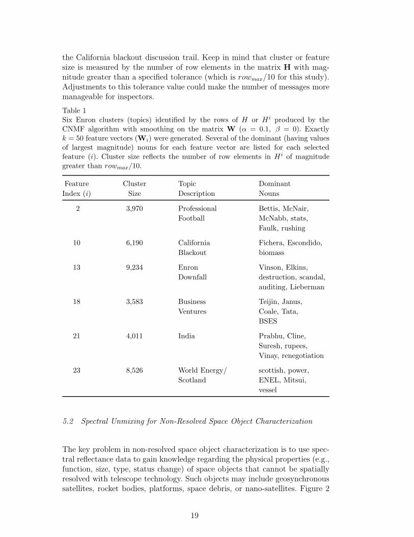
the California blackout discussion trail. Keep in mind that cluster or featuresize is measured by the number of row elements in the matrix H with mag-nitude greater than a specified tolerance (which is rowmax/10 for this study).Adjustments to this tolerance value could make the number of messages moremanageable for inspectors.

Table 1Six Enron clusters (topics) identified by the rows of H or H i produced by theCNMF algorithm with smoothing on the matrix W (α = 0.1, β = 0). Exactlyk = 50 feature vectors (Wi) were generated. Several of the dominant (having valuesof largest magnitude) nouns for each feature vector are listed for each selectedfeature (i). Cluster size reflects the number of row elements in H i of magnitudegreater than rowmax/10.

Feature Cluster Topic Dominant

Index (i) Size Description Nouns

2 3,970 Professional Bettis, McNair,

Football McNabb, stats,

Faulk, rushing

10 6,190 California Fichera, Escondido,

Blackout biomass

13 9,234 Enron Vinson, Elkins,

Downfall destruction, scandal,

auditing, Lieberman

18 3,583 Business Teijin, Janus,

Ventures Coale, Tata,

BSES

21 4,011 India Prabhu, Cline,

Suresh, rupees,

Vinay, renegotiation

23 8,526 World Energy/ scottish, power,

Scotland ENEL, Mitsui,

vessel

5.2 Spectral Unmixing for Non-Resolved Space Object Characterization

The key problem in non-resolved space object characterization is to use spec-tral reflectance data to gain knowledge regarding the physical properties (e.g.,function, size, type, status change) of space objects that cannot be spatiallyresolved with telescope technology. Such objects may include geosynchronoussatellites, rocket bodies, platforms, space debris, or nano-satellites. Figure 2

19

Table 2Top twenty BNC nouns by ascending global entropy weight (gi) and the correspond-ing topics identified among the 50 features (Wi) generated by CNMF using differentvalues of the smoothing parameter α.

Cluster/Topic frequency per α

Noun fi gi .001 .01 .1 .25 .50 .75 1.0 Topic

Waxman 680 0.424 2 2 2 2 2 DownfallLieberman 915 0.426 2 2 2 2 2 Downfallscandal 679 0.428 2 2 2 Downfallnominee 544 0.436 4 3 2 2 2Barone 470 0.437 2 2 2 2 DownfallMeade 456 0.437 2 DownfallFichera 558 0.438 2 2 CA BlackoutPrabhu 824 0.445 2 2 2 2 2 2 IndiaTata 778 0.448 2 Indiarupee 323 0.452 3 4 4 4 3 4 2 Indiasoybean 499 0.455 2 2 2 2 2 2 2rushing 891 0.486 2 2 2 Footballdlrs [dollars] 596 0.487 2Janus 580 0.488 2 3 2 3 Bus. VenturesBSES 451 0.498 2 2 2 Bus. VenturesCaracas 698 0.498 2Escondido 326 0.504 2 2 CA Blackoutpromoters 180 0.509 2 Energy/ScotsAramco 188 0.550 2 Indiadoorman 231 0.598 2

shows an artist’s rendition of a JSAT type satellite in a 36,000 kilometer highsynchronous orbit around the Earth. Even with adaptive optics capabilities,this object is generally not resolvable using ground-based telescope technol-ogy. For safety and other considerations in space, non-resolved space objectcharacterization is an important component of Space Situational Awareness.

Fig. 2. Artist rendition of a JSAT satellite. Image obtained from the Boeing SatelliteDevelopment Center.

Spectral reflectance data of a space object can be gathered using ground-based spectrometers and contains essential information regarding the makeup or types of materials comprising the object. Different materials such asaluminum, mylar, paint, etc. possess characteristic wavelength-dependent ab-

20

sorption features, or spectral signatures, that mix together in the spectralreflectance measurement of an object. Figure 3 shows spectral signatures offour materials typically used in satellites, namely, aluminum, mylar, whitepaint, and solar cell.

0 0.5 1 1.5 20.06

0.065

0.07

0.075

0.08

0.085

0.09

Wavelength, microns

Aluminum

0 0.5 1 1.5 20.072

0.074

0.076

0.078

0.08

0.082

0.084

0.086

Wavelength, microns

Mylar

0 0.5 1 1.5 20

0.05

0.1

0.15

0.2

0.25

0.3

0.35

Wavelength, microns

Solar Cell

0 0.5 1 1.5 20

0.02

0.04

0.06

0.08

0.1

Wavelength, microns

White Paint

Fig. 3. Laboratory spectral signatures for aluminum, mylar, solar cell, and whitepaint. For details see (Luu et al., 2003).

The objective is then, given a set of spectral measurements or traces of anobject, to determine i) the type of constituent materials and ii) the propor-tional amount in which these materials appear. The first problem involvesthe detection of material spectral signatures or endmembers from the spectraldata. The second problem involves the computation of corresponding propor-tional amounts or fractional abundances. This is known as the spectral unmix-

ing problem in the hyperspectral imaging community (Chang, 2000; Keshava,2003; Plaza et al., 2004).

A reasonable assumption for spectral unmixing is that a spectral measurementof an object results from a linear combination of the spectral signatures of itsconstituent materials. Hence in the linear mixing model, a spectral measure-ment of an object y ≥ 0 along m spectral bands is given by y = Uv + n,where U ≥ 0 is an m × k matrix whose columns are the spectral reflectancesignatures of k constituent materials (endmembers), v ≥ 0 is a vector of frac-tional abundances, and n is a noise term. For n spectral measurements we

21

write in block formY = UV + N, (11)

where now Y is the m × n data matrix whose columns are spectral measure-ments, V is a k × n matrix of fractional abundances, and N is noise.

In this section, we apply NMF to the spectral unmixing problem. Specifically,we minimize the extended cost function (3) with A = Y and seek columnvectors in basis matrix W that approximate endmembers in matrix U. Wethen gather the best computed endmembers into a matrix B ≈ U and solvean inverse problem to compute H ≈ V. Other authors have investigated theuse of NMF for spectral unmixing (Plaza et al., 2004). We report on the useof smoothness constraints and the CNMF algorithm presented in Section 4 forimproved extraction of material spectral signatures.

5.3 Simulation Setup

While spectral reflectance data of space objects is being collected at varioussites, such as the Air Force Maui Optical and Supercomputing Site in Maui,HI, publicly disseminated reflectance data of space objects is, to our knowl-edge, not yet available. Hence, like other researchers (Luu et al., 2003), weemployed laboratory-obtained spectral signatures for the creation of simulateddata using the linear mixing model of equation (11).

More specifically, we let U = [u1u2u3u4] where ui are the spectra associatedwith the four materials in Figure 3 measured in the 0.3 to 1.8 micron range,with m = 155 spectral bands. We form the matrix of fractional abundances asV = [V1V2V3V4], where Vi is a 4× 100 matrix whose rows vary sinusoidallywith random amplitude, frequency and phase shift as to model space objectrotation with respect to a fixed detector, but are chosen so that the ith materialspectral signature is dominant in the mixture Yi = UVi + Ni. The noiseis chosen to be 1% Gaussian, that is ‖Ni‖F = 0.01 ∗ ‖Yi‖F/‖Ri‖F wherethe entries in Ri are randomly chosen from a Gaussian distribution N(0, 1).Representative simulated spectral traces from each sub-data set Yi are shownin Figure 4 and are consistent with simulated and real data employed in relatedwork (Luu et al., 2003).

5.4 Numerical Results

We first focus on the problem of endmember determination from the simulatedspectral measurements of Figure 4. To do this, we minimize cost function (3)using algorithm CNMF given in Section 4, with A = [Y1Y2Y3Y4] and with

22

0 0.2 0.4 0.6 0.8 1 1.2 1.4 1.6 1.8 20.06

0.065

0.07

0.075

0.08

0.085

0.09

0.095

0.1

0.105

Wavelength, microns0 0.2 0.4 0.6 0.8 1 1.2 1.4 1.6 1.8 2

0.04

0.06

0.08

0.1

0.12

0.14

0.16

0.18

0.2

Wavelength, microns

0 0.2 0.4 0.6 0.8 1 1.2 1.4 1.6 1.8 20.06

0.065

0.07

0.075

0.08

0.085

0.09

0.095

0.1

0.105

Wavelength, microns0 0.2 0.4 0.6 0.8 1 1.2 1.4 1.6 1.8 2

0.05

0.06

0.07

0.08

0.09

0.1

0.11

0.12

Wavelength, microns

Fig. 4. Representative simulated spectral traces from Yi (i = 1 : 4), where i is thedominant material in the mixture. (top-left) Y1: Aluminum. (top-right) Y2: Mylar.(bottom-left) Y3 Solar cell. (bottom-right) Y4 White paint.

smoothness constraint (4) only in W. The regularization parameter α was setto α = 0 (no auxiliary constraint) and α = 1 (penalize solutions W of largeFrobenius norm). For each value of α we run CNMF with 20 different startingpoints and number of basis k = 6, resulting in a total of 20 candidate (local)solutions W or a set of 120 candidate endmembers {wi}, (i = 1 : 120).

We employ an information theoretic measure to quantitatively evaluate theperformance in endmember extraction of NMF with and without smoothnessconstraints. The measure of choice is Ds(uj ,wi), the symmetric Kullback-Leibler divergence of uj with respect to wi given by

Ds(uj ,wi) = D(uj||wi) + D(uj||wi), (12)

where

D(x||z) =∑

ℓ

x(ℓ)

‖x‖1log(

x(ℓ)‖z‖1

z(ℓ)‖x‖1).

For any nonnegative x and z, the symmetric Kullback-Leibler divergence sat-isfies Ds(x, z) ≥ 0, and the smaller the value of Ds(x, z) the better the match.Thus, for each true endmember uj with j = 1 : 4, we find the best match

23

w∗ ∈ {wi} as,

uj ≈ w∗ = arg mini{Ds(uj ,wi)}.

The scores of the best matches found in {wi} for each of the four materialsare given in Table 3. Values in parentheses corresponds to the scores of bestmatches found with NMF and no auxiliary constraints (α = 0). Notice thatin all cases the scores corresponding to CNMF with α = 1 are lower thanthose obtained with no constraints at all, showing that enforcing smoothnessconstraints can significantly improve the performance of NMF for feature ex-traction.

Table 3Kullback-Leibler divergence scores of the best matching endmembers given by

NMF with and without smoothness constraints. Values in parentheses correspondto standard NMF (no constraints).

Input Aluminum Mylar Solar Cell White Paint

[Y1Y2Y3Y4] 0.0280 0.0659 0.0130 0.0223

(0.1137) (0.0853) (0.0161) (0.0346)

Table 4 shows the scores of the best matches obtained with CNMF whenthe input data matrix to CNMF is A = Yi, rather than A = [Y1Y2Y3Y4].Again scores corresponding to CNMF with α = 1 are generally smaller thanthose obtained with standard NMF. It is interesting to note that for Y3 thesmoothness constraint enabled significantly better performance for aluminumand mylar, at the expense of a slight loss of performance in the determinationof solar cell and white paint.

The visual quality of endmember spectra computed using CNMF with α = 1can be appreciated in Figure 5. Notice that using the Kullback-Leibler diver-gence measure both aluminum and mylar are well represented by the samecomputed endmember spectra.

This result is not surprising as the spectral signatures of aluminum and my-lar are quite similar (see Figure 3). This strong similarity can also be easilyobserved in the confusion matrix shown in Table 5.

Next, we focus on the inverse process of computing fractional abundances giventhe data matrix A = [Y1Y2Y3Y4] and computed material spectral signaturesB ≈ U. Thus we minimize

minH

‖A − BH‖2F , subject to H ≥ 0, (13)

where B ≈ U is formed using computed endmember spectra shown in Fig-

24

Table 4Kullback-Leibler divergence scores of the best matching endmembers given by

NMF with and without smoothness constraints. Values in parentheses correspondto standard NMF (no constraints)

Input (dominant) Aluminum Mylar Solar Cell White Paint

Y1 (Aluminum) 0.0233 0.0124 0.4659 0.1321

(0.0740) (0.0609) (0.6844) (0.1661)

Y2 (Mylar) 0.0165 0.0063 0.4009 0.1203

(0.0615) (0.0606) (0.5033) (0.1827)

Y3 (Solar Cell) 0.0645 0.0292 0.0302 0.2863

(0.1681) (0.1358) (0.0266) (0.1916)

Y4 (White Paint) 0.0460 0.0125 0.8560 0.1735

(0.0882) (0.0571) (0.8481) (0.2845)

0 0.5 1 1.5 20.05

0.06

0.07

0.08

0.09

0.1Best Matched Endmember with Aluminum

0 0.5 1 1.5 20.05

0.06

0.07

0.08

0.09

0.1Best Matched Endmember with Mylar

0 0.5 1 1.5 20

0.05

0.1

0.15

0.2

0.25

0.3

0.35Best Matched Endmember with Solar Cell

0 0.5 1 1.5 20

0.02

0.04

0.06

0.08

0.1

0.12Best Matched Endmember with White Paint

Fig. 5. Plot of the best endmembers extracted using CNMF with α = 1, whoseKullback-Leibler divergence scores appear in Table 3.

ure 5 and selected using the Kullback-Leibler divergence measure of equation(12). We use algorithm PMRNSD (Nagy and Strakos, 2000) for the numericalminimization of (13).

Figure 6 shows the fractional abundances calculated with PMRNSD in blue,compared with the true fractional abundances of matrix V in red. Here alu-

25

Table 5Confusion matrix of the four material spectra in Figure 3. The scores correspondto Ds(ui,uj) for i = 1 : 4 and j = i : 4.

Aluminum Mylar Solar Cell White Paint

Aluminum 0 0.0209 1.2897 0.3317

Mylar - 0 1.2719 0.2979

Solar Cell - - 0 2.5781

White Paint - - - 0

minum and mylar are shown in the same plot since the same computed end-member was selected to represent these materials. The calculated fractionalabundances for solar cell are quite good, while those for the other materials areless accurate. Note that in all cases the relative change of fractional abundanceper observation is well represented by the calculated fractional abundances.

100 200 300 4000

0.2

0.4

0.6

0.8

1

Observations

Per

cent

Aluminum and Mylar

100 200 300 4000

0.2

0.4

0.6

0.8

1

Observations

Per

cent

Solar Cell

100 200 300 4000

0.2

0.4

0.6

0.8

1

Observations

Per

cent

White Paint

Fig. 6. Fractional abundances obtained using PMRNSD with B ≈ U given in Fig-ure 5. True fractional abundances are represented in red. The result of the approx-imation using PMRNSD is in blue.

6 Further Improvements

In this paper, we have attempted to outline some of the major concepts relatedto nonnegative matrix factorization. In addition to developing applications for

26

space object identification and classification and topic detection and trackingin text mining, several open problems with NMF remain. Here are a few ofthem:

• Initializing the factors W and H. Methods for choosing, or seeding, theinitial matrices W and H for various algorithms (see, e.g., (Wild, 2002;Wild et al., 2003; Boutsidis and Gallopoulos, 2005)) is a topic in need offurther research.

• Uniqueness. Sufficient conditions for uniqueness of solutions to the NMFproblem can be considered in terms of simplicial cones (Berman and Plem-mons, 1994), and have been studied in (Donoho and Stodden, 2003). Algo-rithms for computing the factors W and H generally produce local mini-mizers of f(W,H), even when constraints are imposed. It would thus beinteresting to apply global optimization algorithms to the NMF problem.

• Updating the factors. Devising efficient and effective updating methodswhen columns are added to the data matrix A in Equation (1) also ap-pears to be a difficult problem and one in need of further research.

Our plans are thus to continue the study of nonnegative matrix factorizationsand develop further applications to spectral data analysis. Work on applica-tions to air emission quality (Chu et al., 2004) and on text mining (Paucaet al., 2004; Shahnaz et al., 2006) will also be continued.

7 Acknowledgments

The authors would like to thank the anonymous referees for their valuablecomments and suggestions on the original manuscript.

References

Berman, A., Plemmons, R., 1994. Non-Negative Matrices in the MathematicalSciences. SIAM Press Classics Series, Philadelphia, PA.

Berman, G., 1969. Lattice approximations to the minima of functions of severalvariables. Journal of the Association for Computing Machinery 16, 286–294.

Berry, M., Browne, M., 2005a. Email Surveillance Using Nonnegative Ma-trix Factorization. Computational & Mathematical Organization Theory11, 249–264.

Berry, M., Browne, M., 2005b. Understanding Search Engines: MathematicalModeling and Text Retrieval, 2nd Edition. SIAM, Philadelphia, PA.

Bertsekas, D., 1999. Nonlinear Programming. Athena Scientific, Belmont, MA.Boutsidis, C., Gallopoulos, E., 2005. On SVD-based initialization for nonneg-

27

ative matrix factorization. Tech. Rep. HPCLAB-SCG-6/08-05, Universityof Patras, Patras, Greece.

British National Corpus (BNC), 2004. http://www.natcorp.ox.ac.uk.Bro, R., de Jong, S., 1997. A fast non-negativity constrained linear least

squares algorithm. Journal of Chemometrics 11, 393–401.Catral, M., Han, L., Neumann, M., Plemmons, R., 2004. On reduced rank non-

negative factorization for symmetric non-negative matrices. Linear Algebraand Applications 393, 107–126.

Cea, J., 1971. Optimisation: Theorie et algorithmes. Dunod, Paris.Chang, C.-I., 2000. An information theoretic-based approach to spectral vari-

ability, similarity, and discriminability for hyperspectral image analysis.IEEE Trans. Information Theory 46, 1927–1932.

Chen, Z., Cichocki, A., 2005. Nonnegative matrix factorization with temporalsmoothness and/or spatial decorrelation constraints. Preprint.

Chu, M., Diele, F., Plemmons, R., Ragni, S., 2004. Optimality, computa-tion, and interpretations of nonnegative matrix factorizations, available athttp://www.wfu.edu/∼plemmons.

Cichocki, A., Zdunek, R., 2006. NMFLAB for Signal Processing, available athttp://www.bsp.brain.riken.jp/ICALAB/nmflab.html.

Cichocki, A., Zdunek, R., Amari, S., March 5-8 2006. Csiszar’s divergences fornon-negative matrix factorization: Family of new algorithms. In: Proc. 6thInternational Conference on Independent Component Analysis and BlindSignal Separation. Charleston, SC.

de Leeuw, J., Young, F., Takane, Y., 1976. Additive structure in qualitativedata: an alternating least squares method with optimal scaling features.Psychometrika 41, 471–503.

Dhillon, I., Sra, S., 2005. Generalized nonnegative matrix approximations withbregman divergences. In: Proceeding of the Neural Information ProcessingSystems (NIPS) Conference. Vancouver, B.C.

Ding, C., he, X., Simon, H., 2005. On the Equivalence of Nonnegative MatrixFactorization and Spectral Clustering. In: Proceedings of the Fifth SIAMInternational Conference on Data Mining. Newport Beach, CA.

Donoho, D., Stodden, V., 2003. When does non-negative matrix factorizationgive a correct decomposition into parts? In: Seventeenth Annual Conferenceon Neural Information Processing Systems.

Drineas, P., Kannan, R., Mahoney, M., 2006. Fast monte carlo algorithms formatrices iii: Computing a a compressed approximate matrix decomposition.SIAM Journal on Computing. To appear.

Finesso, L., Spreij, P., July 5-9 2004. Approximate nonnegative matrix factor-ization via alternating minimization. In: Proc. 16th International Sympo-sium on Mathematical Theory of Networks and Systems. Leuven, Belgium.

Gill, P., Murray, W., Wright, M., 1981. Practical Optimization. AcademicPress, London.

Gonzalez, E., Zhang, Y., March 2005. Accelerating the Lee-Seung algorithmfor nonnegative matrix factorization. Tech. Rep. TR-05-02, Rice University.

28

Grieve, T., October 14 2003. The Decline and Fall of the Enron Empire. Slatehttp://www.salon.com/news/feature/2003/10/14/enron/index np

.html.Grippo, L., Sciandrone, M., 2000. On the convergence of the block nonlinear

gauss-seidel method under convex constraints. Operations Research Letters26 (3), 127–136.

Guillamet, D., Bressan, M., Vitria, J., 2001. A weighted non-negative matrixfactorization for local representations. In: Proc. 2001 IEEE Computer Soci-ety Conference on Computer Vision and Pattern Recognition. Vol. 1. Kavai,HI, pp. 942–947.

Hamza, A. B., Brady, D., 2006. Reconstruction of reflectance spectra usingrobust non-negative matrix factorization. To appear.

Hoyer, P., 2002. Non-Negative Sparse Coding. In: Proceedings of the IEEEWorkshop on Neural Networks for Signal Processing. Martigny, Switzerland.

Hoyer, P., 2004. Non-negative Matrix Factorization with Sparseness Con-straints. J. of Machine Learning Research 5, 1457–1469.

Karvanen, J., Cichocki, A., 2003. Measuring Sparseness of Noisy Signals. In:Proceedings of the Fourth International Symposium on Independent Com-ponent Analysis and Blind Signal Separation (ICA2003). Nara, Japan.

Keila, P., Skillicorn, D., 2005. Detecting unusual and deceptive communicationin email. Tech. rep., School of Computing, Queen’s University, Kingston,Ontario, Canada.

Keshava, N., 2003. A survey of spectral unmixing algorithms. Lincoln Labo-ratory Journal 14 (1), 55–77.

Langville, A., Meyer, C., Albright, R., Cox, J., Duling, D., 2006. Algorithms,initializations, and convergence for the nonnegative matrix factorization,preprint.

Lawson, C., Hanson, R., 1995. Solving Least Squares Problems. SIAM,Philadelphia, PA.

Lee, D., Seung, H., 1999. Learning the Parts of Objects by Non-NegativeMatrix Factorization. Nature 401, 788–791.

Lee, D., Seung, H., 2001. Algorithms for Non-Negative Matrix Factorization.Advances in Neural Information Processing Systems 13, 556–562.

Lin, C.-J., 2005a. On the convergence of multiplicative update algorithms fornon-negative matrix factorization. Tech. Rep. Information and Support Ser-vices Techincal Report, Department of Computer Science, National TaiwanUniversity.

Lin, C.-J., 2005b. Projected gradient methods for non-negative matrix fac-torization. Tech. Rep. Information and Support Services Technical ReportISSTECH-95-013, Department of Computer Science, National Taiwan Uni-versity.

Luu, K., Matson, C., Snodgrass, J., Giffin, M., Hamada, K., Lambert, J., Sept.2003. Object characterization from spectral data. In: Proc. 2003 AMOSTechnical Conference. Maui, HI.

McLean, B., Elkind, P., 2003. The Smartest Guys in the Room: The Amazing

29

Rise and Scandalous Fall of Enron. Portfolio.Nagy, J. G., Strakos, Z., 2000. Enforcing nonnegativity in image reconstruction

algorithms. Mathematical Modeling, Estimation, and Imaging 4121, 182–190.

Nocedal, J., Wright, S., 1999. Numerical Optimization. Springer.Paatero, P., 1997. Least squares formulation of robust non-negative factor

analysis. Chemometrics and Intelligent Laboratory Systems 37, 23–35.Paatero, P., 1999. The multilinear engine—a table-driven least squares pro-

gram for solving multilinear problems, including the n-way parallel factoranalysis model. Journal of Computational and Graphical Statistics 8 (4),1–35.

Paatero, P., Tapper, U., 1994. Positive matrix factorization: A non-negativefactor model with optimal utilization of error estimates of data values. En-vironmetrics 5, 111–126.

Pauca, P., Piper, J., Plemmons, R., 2005. Nonnegative matrix factorizationfor spectral data analysis. Linear Algebra and Its Applications In press,available at http://www.wfu.edu/∼plemmons.

Pauca, V., Plemmons, R., Abercromby, K., 2006. Nonnegative matrix factor-ization methods with physical constraints for spectral unmixing. In prepa-ration.

Pauca, V., Shahnaz, F., Berry, M., Plemmons, R., 2004. Text Mining UsingNon-Negative Matrix Factorizations. In: Proceedings of the Fourth SIAMInternational Conference on Data Mining, April 22-24. SIAM, Lake BuenaVista, FL.

Piper, J., Pauca, V., Plemmons, R., Giffin, M., Sept. 2004. Object character-ization from spectral data using nonnegative factorization and informationtheory. In: Proc. 2004 AMOS Technical Conference. Maui, HI.

Plaza, A., Martinez, P., Perez, R., Plaza, J., 2004. A quantitative and com-parative analysis of endmember extraction algorithms from hyperspectraldata. IEEE Trans. on Geoscience and Remote Sensing 42 (3), 650–663.

Polak, E., 1971. Computational Methods in Optimization: a unified approach.Academic Press, New York.

Powell, M., 1964. An efficient method for finding the minimum of a functionof several variables without calculating derivatives. The Computer Journal7, 155–162.

Powell, M., 1973. On search directions for minimization. Mathematical Pro-gramming 4, 193–201.

Salakhutdinov, R., Roweis, S. T., Ghahramani, Z., 2003. On the convergenceof bound optimization algorithms. Uncertainty in Artificial Intelligence 19,509–516.

Shahnaz, F., Berry, M., Pauca, V., Plemmons, R., 2006. Document clusteringusing nonnegative matrix factorization. Information Processing & Manage-ment 42 (2), 373–386.

Smilde, A., Bro, R., Geladi, P., 2004. Multi-way Analysis. Wiley, West Sussex,England.

30

Torczon, V., 1997. On the convergence of pattern search algorithms. SIAMJournal on Optimization 7, 1–25.

Wang, Y., Jiar, Y., Hu, C., Turk, M., January 27-30 2004. Fisher non-negativematrix factorization for learning local features. In: Asian Conference onComputer Vision. Korea.

Wild, S., 2002. Seeding non-negative matrix factorization with the sphericalk-means clustering. Master’s thesis, University of Colorado.

Wild, S., Curry, J., Dougherty, A., 2003. Motivating Non-Negative Ma-trix Factorizations. In: Proceedings of the Eighth SIAM Conferenceon Applied Linear Algebra, July 15-19. SIAM, Williamsburg, VA,http://www.siam.org/meetings/la03/proceedings.

Wold, H., 1966. Nonlinear estimation by iterative least squares procedures. In:David, F. (Ed.), Research Papers in Statistics. John Wiley and Sons, Inc.,New York, pp. 411–444.

Wold, H., 1975. Soft modelling by latent variables: nonlinear iterative partialleast squares approach. In: Gani, J. (Ed.), Perspectives in Probability andStatistics. Academic Press, London, pp. 411–444.

Xu, W., Liu, X., Gong, Y., 2003. Document-Clustering based on Non-NegativeMatrix Factorization. In: Proceedings of SIGIR’03, July 28-August 1.Toronto, CA, pp. 267–273.

Zangwill, W., 1967. Minimizing a function without calculating derivatives.The Computer Journal 10, 293–296.

Zdunek, R., Cichocki, A., June 25-29 2006. Non-negative matrix factorizationwith quasi-newton optimization. In: Proc. Eighth International Conferenceon Artificial Intelligence and Soft Computing, ICAISC. Zakopane, Poland.

31