algorithms for computing quartic galois groups over …facstaff.elon.edu/cawtrey/abk-quartic.pdf ·...

ALGORITHMS FOR COMPUTING QUARTIC GALOIS GROUPS

OVER FIELDS OF CHARACTERISTIC 0

CHAD AWTREY, JAMES BEUERLE, AND MICHAEL KEENAN

Abstract. Let f(x) be an irreducible degree four polynomial defined over

a field F and let K = F (↵) where ↵ is a root of f in some fixed algebraic

closure F of F . Several methods appear in the literature for computing theGalois group G of f , most of which rely on forming and factoring resolvent

polynomials; i.e., polynomials defining subfields of the splitting field of f .This paper surveys those methods that generalize to arbitrary base fields ofcharacteristic 0. Further, we describe a non-resolvent method that determines

if K has a quadratic subfield by counting the number of roots of f that are

contained in K, and we also describe how to construct explicitly a polynomialdefining a quadratic subfield. We end with a comparison of run times for the

various algorithms in the case F is the rational numbers.

1. Introduction

Galois theory shows it is possible to associate a group structure to a polynomial’sroots. This group, called the polynomial’s Galois group, is a collection of permuta-tions of the roots that encodes arithmetic information concerning the polynomial.For example, the polynomial is solvable by radicals if and only if its Galois groupis solvable (see for example [4, p.628]). An important problem in computationalalgebra therefore is to determine the Galois group of a polynomial f(x) of degreen defined over a field F .

For this paper, we focus on quartic polynomials, surveying methods appearing inthe literature that apply to arbitrary base fields of characteristic 0. These methods[1,3,4,7] rely on factoring resolvent polynomials [5,8,9], which are polynomials thatdefine subfields of the splitting field of f . We also present a non-resolvent methodthat relies on factoring the quartic polynomial over the extension field it defines.One advantage of this method is that it allows us to determine when the quarticpolynomial’s extension field has a quadratic subfield, and it gives us an explicitcalculation of a polynomial that defines such a quadratic subfield. As a corollary,we can determine when any irreducible quartic polynomial can be transformed intoa biquadratic (i.e., even quartic) polynomial defining the same extension, and hencehaving the same Galois group.

The remainder of the paper is organized as follows. Section 2 provides a briefoverview of the basic notation and terminology related to the Fundamental Theo-rem of Galois Theory as they relate to our context. In this section, we also show therelationship between the automorphism group of a polynomial’s extension field and

2010 Mathematics Subject Classification. 12Y05, 20B35, 12F10.Key words and phrases. quartic Galois groups; resolvent polynomials; automorphism groups;

e�ciency.

1

2 CHAD AWTREY, JAMES BEUERLE, AND MICHAEL KEENAN

its Galois group, paving the way for our non-resolvent approach to computing quar-tic Galois groups. In Section 3 we give an introduction to resolvent polynomials,including a discussion of the most widely-used resolvent; namely, the discriminant.Section 4 details all of the algorithms under consideration that are based on theresolvent method. For each algorithm, we describe its implementation and prove itscorrectness. Section 5 discusses our non-resolvent algorithm for computing quarticGalois groups. Additionally, we show every biquadratic irreducible quartic polyno-mial has a Galois group that is a subgroup of D4 (the dihedral group of order 8).Conversely, if a quartic polynomial’s Galois group is a subgroup of D4, we describehow to construct explicitly a biquadratic polynomial that defines the same exten-sion (and hence has the same Galois group). Our final section includes an analysisof run times for each algorithm considered in this paper in the case the ground fieldis the rational numbers. Our findings indicate that the most e�cient algorithm isthe modification of the traditional cubic resolvent method, as outlined in [7].

2. Overview of Galois Theory

In this section, we give a very brief overview of Galois theory in our context.More details can be found in any standard text on abstract algebra (such as [4]).

Let F be a field and let F be a fixed algebraic closure. Let f(x) 2 F [x] be anirreducible polynomial of degree n with roots ↵ = ↵1, . . . ,↵n 2 F . Let K be thestem field of f ; that is, K = F (↵).

Then it is straight forward to verify that K is a vector space over F with the set{1,↵, . . . ,↵�1

} serving as a basis. Since the dimension of K as an F -vector spaceis n, we say K/F is an extension field of degree n and we write [K : F ] = n.

We are interested primarily in automorphisms of K/F , which are field isomor-phisms from K to itself that restrict to the identity function on F .

Definition 2.1. An automorphism of K/F is a mapping � : K ! K such that,

(1) � is bijective,(2) �(x+ y) = �(x) + �(y) for all x, y 2 K,(3) �(xy) = �(x)�(y) for all x, y 2 K,(4) �(a) = a for all a 2 F .

The collection of all automorphisms of K/F is denoted Aut(K/F ).

The automorphisms of K/F form a group under function composition. Sinceautomorphisms are field isomorphisms and since a basis for K/F consists of powersof the one root ↵, it follows that each automorphism is completely determined bywhere it sends ↵. Furthermore, since automorphisms act like the identity functionon F , we have 0 = �(0) = �(f(↵)) = f(�(↵)) for each � 2 Aut(K/F ). This showsthat automorphisms send ↵ to some other root of f that lies in K.

Therefore, elements in Aut(K/F ) are in a bijective correspondence with the rootsof f that are contained in K, and each automorphism permutes these roots. In thecase where K contains all n roots of f , Aut(K/F ) is called the Galois group off . Otherwise, the Galois group of f is the automorphism group of the splittingfield of f ; that is, the smallest subfield of F that contains F and all n roots of f .

The Fundamental Theorem. The next result is the Fundamental Theorem ofGalois Theory, which gives a bijection between the subfields of K/F and the sub-groups of Aut(K/F ) when K/F is a Galois extension (see [4, p. 574]).

QUARTIC GALOIS GROUPS 3

Theorem 2.2 (Fundamental Theorem of Galois Theory). Let L be the splittingfield of an irreducible polynomial f of degree n defined over F , and let G be theGalois group of f (i.e., the automorphism group of L/F ). There is a bijectivecorrespondence between the subfields of L/F and the subgroups of G. Specifically,if K is a subfield of L/F , then K corresponds to the set of all � 2 G such that�(a) = a for all a 2 K. Similarly, if H is a subgroup of G, then H corresponds tothe set of all a 2 L such that �(a) = a for all � 2 H.

The Galois correspondence has the following properties.

(1) If H1 and H2 are subgroups of G that correspond to subfields K1 and K2

respectively, then H1 H2 if and only if K2 ✓ K1.(2) If K defines a subfield of L of degree d over F , then K corresponds to a

subgroup H G of index d.(3) Let K be a subfield of L/F defined by the polynomial g and let H G be

the subgroup corresponding to K. The splitting field of g corresponds to thelargest normal subgroup N of G contained inside H; i.e., the kernel of thepermutation representation of G acting on G/H. The Galois group of g isisomorphic to G/N .

(4) If we label the roots of f as ↵1, . . . ,↵n, then G can be identified with atransitive subgroup of Sn, well-defined up to conjugation.

(5) If we label the roots of f as ↵1, . . . ,↵n, then the stem field of f (generatedby ↵1) corresponds to G1, the point stabilizer of 1 inside G.

Automorphism Groups and Stem Fields. We now prove several facts aboutsubfields of L/F and subgroups of Aut(L/F ). The first considers conjugate fieldsof a subfield K of L/F . For � 2 Aut(L/F ) and a subfield K of L/F , the image�(K) of K under � is called a conjugate field of K. The next result shows thatconjugate fields correspond to conjugate subgroups.

Proposition 2.3. Let L/F be a Galois extension with Galois group G. Let H bea subgroup of G and let K be the fixed field of H. For � 2 G, the subgroup fixing�(K) is �H��1.

Proof. First we show �H��1 fixes �(K). Let �h��12 �H��1 and let �(x) 2 �(K).

Then �h��1(�(x)) = �h(x) = �(x), as desired.Next we show every element that fixes �(K) belongs to �H��1. Suppose ⌧ 2 G

fixes �(K). Then for all x 2 K, ⌧(�(x)) = �(x). Thus ��1⌧�(x) = x. Thus ��1⌧�fixes K, which implies ��1⌧� 2 H. Thus ⌧ 2 �H��1, as desired. ⇤Proposition 2.4. Let L/F be a Galois extension with Galois group G. Let H bea subgroup of G and let K be the fixed field of H. Let �, ⌧ 2 G. Then �(x) = ⌧(x)for all x 2 K if and only if ⌧ 2 �H.

Proof. Let �, ⌧ 2 G and suppose �(x) = ⌧(x) for all x 2 K. Then x = ��1⌧(x) forall x 2 K. Thus ��1⌧ fixes K, which is true if and only if ��1⌧ 2 H. This is trueif and only if ⌧ 2 �H, as desired. ⇤

Next we describe the relationship between the automorphism group of a subfieldand the Galois group of the splitting field.

Proposition 2.5. Let L/F be a Galois extension with Galois group G. Let H bea subgroup of G and let K be the fixed field of H. Then Aut(K/F ) ' N/H, whereN is the normalizer of H in G.


Table 1. The 5 conjugacy classes of transitive subgroups of S4.Generators are for one representative in each conjugacy class.

T Name Generators Size

1 C4 (1234) 4

2 V4 (12)(34), (13)(24) 4

3 D4 (1234), (13) 8

4 A4 (123), (234) 12

5 S4 (1234), (12) 24

Proof. First we note that every element in Aut(K/F ) corresponds to some restric-tion to K of an element � 2 G [4, p. 575]. Such an element � will restrict to anautomorphism of K/F precisely when �(K) = K. By Proposition 2.3, these arerestrictions of elements in the normalizer N of H in G. By Proposition 2.4, the ele-ments in N that restrict to distinct functions on K correspond to the cosets of H inN . Therefore Aut(K/F ) is isomorphic to the quotient group N/H, as desired. ⇤

As a corollary, the next result explicitly determines the connection between theautomorphism group of a polynomial’s stem field and the polynomial’s Galois group.This will be the basis for our non-resolvent method for computing quartic Galoisgroups, as mentioned in Section 5.

Corollary 2.6. Let L be the splitting field of the irreducible polynomial f(x) ofdegree n defined over F , and let G be the Galois group of f . Let K/F be the stemfield of f . Let G1 be the point stabilizer of 1 inside G, and let N be the normalizerof G1 in G. Then Aut(K/F ) ' N/G1. Furthermore, the number of roots of f thatare contained in K is equal to the index [N : G1].

Proof. Since K is the stem field, K ' F (↵1), where ↵1, . . . ,↵n are the roots off in F . Under the Galois correspondence, the subgroup that corresponds to Kconsists of those elements that fix K; i.e., all � 2 G such that �(↵1) = ↵1. Thisis precisely the point stabilizer of 1 inside G. Therefore Aut(K/F ) ' N/G1 byProposition 2.5. In particular, these two groups have the same order. The finalstatement of the corollary now follows since the number of automorphisms equalsthe number of roots of f contained in K, and the number of elements in N/G1 isequal to the index [N : G1]. ⇤

Notice that by item (4) of Theorem 2.2, we must identify the conjugacy classesof transitive subgroups of S4 in order to determine the group structure of G. Thisinformation is well known (see [2]). In Table 1, we give information on the 5conjugacy classes of transitive subgroups of S4, including their transitive number(or T-number, as in [6]), generators of one representative, their size, and a moredescriptive name based on their structure. The descriptive names are standard: C4

represents the cyclic group of order n, D4 the dihedral group of order 8, V4 theelementary abelian group of order 4, and A4 and S4 the alternating and symmetricgroups on 4 letters.

3. Resolvent Polynomials and Splitting Fields

The techniques for computing Galois groups this paper is studying are basedon the use of absolute resolvent polynomials [8]. In short, this method works asfollows. Let f(x) be an irreducible polynomial (over F ) of degree n. Let G be the


Galois group of f , and let H be a subgroup of Sn. We form a resolvent polynomialRH(x) whose stem field corresponds to H under the Galois correspondence. Byitem (3) of Theorem 2.2, the Galois group of RH(x) is isomorphic to the image ofthe permutation representation of G acting on the cosets Sn/H. Then as shownin [8], the irreducible factors of RH(x) therefore correspond to the orbits of thisaction. In particular, the degrees of the irreducible factors correspond to the orbitlengths.

The most di�cult task in the resolvent method is constructing the polynomialRH(x) that corresponds to a given subgroup H of Sn. The following result givesone method for accomplishing such a task. A proof can be found in [8].

Theorem 3.1. Let f(x) be an irreducible polynomial of degree n defined over a fieldF , K the splitting field of f , and ↵1, . . . ,↵n the roots of f in F . Let T (x1, . . . , xn)be a polynomial with coe�cients in F , and let H be the stabilizer of T in Sn. Thatis

H = {� 2 Sn : T (x�(1), . . . , x�(n)) = T (x1, . . . , xn)}.

Let Sn//H denote a complete set of coset representatives of H in Sn, and definethe resolvent polynomial RH(x) by:

RH(x) =Y

�2Sn//H

(x� T (↵�(1), . . . ,↵�(n))).

(1) If RH(x) is squarefree, its Galois group is isomorphic to the image of thepermutation representation of G acting on the cosets Sn/H.

(2) We can ensure RH(x) is squarefree by taking a suitable Tschirnhaus trans-formation of f(x) [3, p.324]. This amounts to randomly picking an elementin the stem field of f(x) and computing its characteristic polynomial.

(3) One choice for T is given by:

T (x1, . . . , xn) =X

�2H

nY

i=1

xi�(i)

!.

Though this is not the only choice.

We now describe how to construct the resolvents used in the following papers:[1, 3, 7]. To illustrate each of these constructions, we will use the following samplepolynomials:

t1 x4 + 5x2 + 5t2 x4 + 1t3 x4 + 2t4 x4

� 7x2� 3x+ 1

t5 x4� x3 + 1

The Discriminant. Perhaps the most well known example of a resolvent poly-nomial is the discriminant. Recall that the discriminant of a degree n polynomialf(x) is given by

disc(f) =Y

1i<jn

(↵i � ↵j)2,

where ↵i are the roots of f . In particular, let

T =Y

1i<jn

(xi � xj).


It is well-known that T is stabilized by An [4, p.610]. Notice that a completeset of coset representatives of Sn/An is {id, (12)}. Also notice that applying thepermutation (12) to the subscripts of T results in �T . In this case, we can formthe resolvent polynomial R(x) as follows,

R(x) =Y

�2Sn/An

(x� �(T )) = x2� T 2 = x2

� disc(f).

In particular, this resolvent factors if and only if the discriminant is a perfect squarein the base field. It is well-known that the discriminant can be computed via theresultant of f(x) and its derivative; namely, disc(f) = (�1)n(n�1)Res(f, f 0) [3, p.119].

Furthermore, by the theory of elementary symmetric polynomials, it follows thatdisc(f) can be expressed using only the coe�cients of f [4, p. 611]. For example,in the case of quartic polynomials,we have:

disc(x4 + ax3 + bx2 + cx+ d) = �27a4d2 + 2a3c(9bd� 2c2)

� a2(4b3d� b2c2 � 144bd2 + 6c2d)

� 2ac(40b2d� 9bc2 + 96d2)

+ 4b(4b3 � b2c2 � 32bd2 + 36c2d)

� 27c4 + 256d3.

Here are the discriminants of the five sample polynomials t1, . . . , t5; the finalcolumn gives the prime factorization of the discriminant over the rational numbers.

Poly Disc Factorizationt1 2000 24.53

t2 256 28

t3 2048 211

t4 33489 32.612

t5 229 2291

The Cubic Resolvent. Both the traditional approach to computing quartic Ga-lois groups [4, p. 614] and its refinement [7] rely on factoring a cubic resolventpolynomial. In this case, we let T = x1x3 + x2x4. The stabilizer H of T in S4 is adihedral group of order 8. The elements of this particular group are,

H = {(1), (13), (24), (12)(34), (13)(24), (14)(23), (1234), (1432)} .

A complete set of right coset representatives for S4/H is given by: {(1), (12), (14)}.We can form the cubic resolvent for f(x) by computing RH :

RH(x) = (x� (↵1↵3 + ↵2↵4)) (x� (↵2↵3 + ↵1↵4)) (x� (↵4↵3 + ↵2↵1)) .

We can also express the cubic resolvent in terms of the coe�cients of the originalquartic. If f(x) = x4 + ax3 + bx2 + cx+ d, then the cubic resolvent of f is:

RH(x) = x3� bx2 + (ac� 4d)x+ 4bd� a2d� c2

Here are the cubic resolvents of the five sample polynomials t1, . . . , t5; the finalcolumn gives the factorization of the cubic resolvent over the rational numbers.


Poly Cubic Res Factorizationt1 x3

� 5x2� 20x+ 100 (x2

� 20)(x� 5)t2 x3

� 4x x(x� 2)(x+ 2)t3 x3

� 8x x(x2� 8)

t4 x3 + 7x2� 4x� 37 x3 + 7x2

� 4x� 37t5 x3

� 4x� 1 x3� 4x� 1

The Degree 6 Resolvent. The method in [3, §6.3] relies on factoring a degree 6resolvent polynomial. In this case, we let T = (x1+x3�(x2+x4))(x1�x3)(x2�x4).The stabilizer H of T in S4 is a cyclic group of order 4. The elements of thisparticular group are,

H = {(1), (1234), (13)(24), (1432)} .

A complete set of right coset representatives for S4/H is given by:

{(1), (12), (13), (14), (23), (34)}.

We can form the degree 6 resolvent for f(x) by computing RH :

RH(x) =Y

�2S4/H

(x� (↵�(1)+↵�(3)� (↵�(2)+↵�(4)))(↵�(1)�↵�(3))(↵�(2)�↵�(4))).

We can also express the degree 6 resolvent in terms of the coe�cients of the originalquartic. If f(x) = x4 + ax3 + bx2 + cx+ d, then the degree 6 resolvent of f is:

RH(x) = x6 +Ax4 +Bx2 + C,

where

A = �2a2b2 + 8b3 + 6a3c� 28abc+ 36c2 + 12a2d� 32bdB = a4b4�8a2b5+16b6�6a5b2c+52a3b3c�112ab4c+9a6c2�84a4bc2+156a2b2c2+

160b3c2+124a3c3�576abc3+432c4�12a4b2d+96a2b3d�192b4d+36a5cd�336a3bcd+768ab2cd+240a2c2d�1152bc2d+144a4d2�768a2bd2+768b2d2+768acd2 � 1024d3

C = �a8b2c2 +12a6b3c2 � 48a4b4c2 +64a2b5c2 +4a9c3 � 50a7bc3 +192a5b2c3 �160a3b3c3�256ab4c3+91a6c4�760a4bc4+1520a2b2c4+256b3c4+688a3c5�2880abc5 + 1728c6 + 4a8b3d� 48a6b4d+ 192a4b5d� 256a2b6d� 18a9bcd+224a7b2cd � 864a5b3cd + 768a3b4cd + 1024ab5cd + 6a8c2d � 480a6bc2d +3680a4b2c2d�7168a2b3c2d�1024b4c2d+96a5c3d�3840a3bc3d+14336ab2c3d+384a2c4d � 9216bc4d + 27a10d2 � 360a8bd2 + 1712a6b2d2 � 3328a4b3d2 +2048a2b4d2+624a7cd2�5568a5bcd2+14336a3b2cd2�8192ab3cd2+4800a4c2d2�21504a2bc2d2+8192b2c2d2+12288ac3d2�256a6d3+2048a4bd3�4096a2b2d3�4096a3cd3 + 16384abcd3 � 16384c2d3

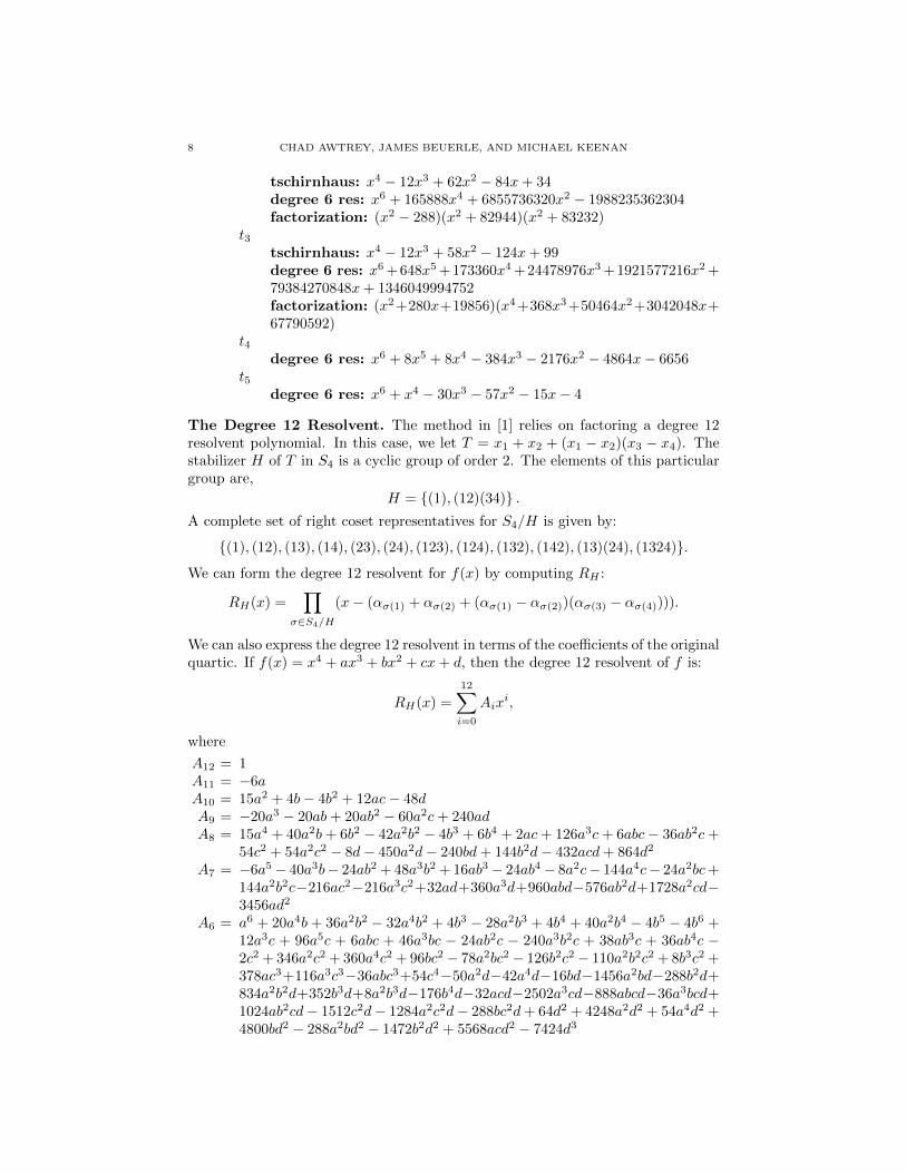
Here are the degree 6 resolvents of the five sample polynomials t1, . . . , t5. Notethat we need to take a tschirnhaus transformation of t1, t2, and t3, since their degree6 resolvents are not squarefree. In each case, we give the transformed polynomial,the degree 6 resolvent, and the factorization of the degree 6 polynomial over therationals. For t4 and t5, the resolvent is irreducible, so we only give it.

t1tschirnhaus: x4 + 8x3 + 34x2 + 32x+ 181degree 6 res: x6

� 8388608000x2� 214748364800000

factorization: (x� 320)(x+ 320)(x4 + 102400x2 + 2097152000)t2


tschirnhaus: x4� 12x3 + 62x2

� 84x+ 34degree 6 res: x6 + 165888x4 + 6855736320x2

� 1988235362304factorization: (x2

� 288)(x2 + 82944)(x2 + 83232)t3


� 124x+ 99degree 6 res: x6+648x5+173360x4+24478976x3+1921577216x2+79384270848x+ 1346049994752factorization: (x2+280x+19856)(x4+368x3+50464x2+3042048x+67790592)

t4degree 6 res: x6 + 8x5 + 8x4

� 384x3� 2176x2

� 4864x� 6656t5

degree 6 res: x6 + x4� 30x3

� 57x2� 15x� 4

The Degree 12 Resolvent. The method in [1] relies on factoring a degree 12resolvent polynomial. In this case, we let T = x1 + x2 + (x1 � x2)(x3 � x4). Thestabilizer H of T in S4 is a cyclic group of order 2. The elements of this particulargroup are,

H = {(1), (12)(34)} .

A complete set of right coset representatives for S4/H is given by:

{(1), (12), (13), (14), (23), (24), (123), (124), (132), (142), (13)(24), (1324)}.

We can form the degree 12 resolvent for f(x) by computing RH :

RH(x) =Y

�2S4/H

(x� (↵�(1) + ↵�(2) + (↵�(1) � ↵�(2))(↵�(3) � ↵�(4)))).

We can also express the degree 12 resolvent in terms of the coe�cients of the originalquartic. If f(x) = x4 + ax3 + bx2 + cx+ d, then the degree 12 resolvent of f is:

RH(x) =12X

i=0

Aixi,

where

A12 = 1A11 = �6aA10 = 15a2 + 4b� 4b2 + 12ac� 48dA9 = �20a3 � 20ab+ 20ab2 � 60a2c+ 240adA8 = 15a4 + 40a2b+ 6b2 � 42a2b2 � 4b3 + 6b4 + 2ac+ 126a3c+ 6abc� 36ab2c+

54c2 + 54a2c2 � 8d� 450a2d� 240bd+ 144b2d� 432acd+ 864d2

A7 = �6a5 � 40a3b� 24ab2 +48a3b2 +16ab3 � 24ab4 � 8a2c� 144a4c� 24a2bc+144a2b2c�216ac2�216a3c2+32ad+360a3d+960abd�576ab2d+1728a2cd�3456ad2

A6 = a6 + 20a4b + 36a2b2 � 32a4b2 + 4b3 � 28a2b3 + 4b4 + 40a2b4 � 4b5 � 4b6 +12a3c + 96a5c + 6abc + 46a3bc � 24ab2c � 240a3b2c + 38ab3c + 36ab4c �2c2 +346a2c2 +360a4c2 +96bc2 � 78a2bc2 � 126b2c2 � 110a2b2c2 +8b3c2 +378ac3+116a3c3�36abc3+54c4�50a2d�42a4d�16bd�1456a2bd�288b2d+834a2b2d+352b3d+8a2b3d�176b4d�32acd�2502a3cd�888abcd�36a3bcd+1024ab2cd� 1512c2d� 1284a2c2d� 288bc2d+ 64d2 + 4248a2d2 + 54a4d2 +4800bd2 � 288a2bd2 � 1472b2d2 + 5568acd2 � 7424d3


A5 = �4a5b�24a3b2+12a5b2�12ab3+28a3b3�12ab4�36a3b4+12ab5+12ab6�8a4c�36a6c�18a2bc�54a4bc+72a2b2c+216a4b2c�114a2b3c�108a2b4c+6ac2 � 282a3c2 � 324a5c2 � 288abc2 + 234a3bc2 + 378ab2c2 + 330a3b2c2 �24ab3c2�1134a2c3�348a4c3+108a2bc3�162ac4+38a3d�126a5d+48abd+1008a3bd+864ab2d� 486a3b2d� 1056ab3d� 24a3b3d+528ab4d+96a2cd+1458a4cd + 2664a2bcd + 108a4bcd � 3072a2b2cd + 4536ac2d + 3852a3c2d +864abc2d�192ad2�648a3d2�162a5d2�14400abd2+864a3bd2+4416ab2d2�16704a2cd2 + 22272ad3

A4 = 6a4b2�2a6b2+12a2b3�16a4b3+b4+10a2b4+19a4b4+4b5�16a2b5+6b6�14a2b6+4b7+b8+2a5c+6a7c+18a3bc+36a5bc+6ab2c�72a3b2c�114a5b2c�10ab3c+148a3b3c�50ab4c+126a3b4c�46ab5c�12ab6c�5a2c2+126a4c2+171a6c2 � 4bc2 + 302a2bc2 � 300a4bc2 + 34b2c2 � 345a2b2c2 � 393a4b2c2 +64b3c2+248a2b3c2+10b4c2+58a2b4c2�16b5c2+42ac3+1342a3c3+438a5c3�306abc3�548a3bc3�180ab2c3�136a3b2c3+120ab3c3+513c4+1215a2c4+129a4c4� 540bc4� 216a2bc4� 108b2c4+324ac5� 14a4d+84a6d� 52a2bd�252a4bd�8b2d�974a2b2d�12a4b2d�96b3d+1344a2b3d+60a4b3d�56b4d�734a2b4d+144b5d� 16a2b5d+112b6d� 8acd� 102a3cd+36a5cd+8abcd�3522a3bcd � 270a5bcd + 240ab2cd + 4044a3b2cd � 784ab3cd + 120a3b3cd �

944ab4cd � 168c2d � 3846a2c2d � 3636a4c2d � 2880bc2d � 3144a2bc2d �

216a4bc2d+5040b2c2d+2280a2b2c2d+384b3c2d� 6480ac3d� 1416a3c3d�864abc3d � 1296c4d + 16d2 + 120a2d2 � 2367a4d2 + 405a6d2 + 320bd2 +14784a2bd2 � 2700a4bd2 + 5280b2d2 + 912a2b2d2 � 108a4b2d2 � 8512b3d2 +384a2b3d2 + 1120b4d2 � 2976acd2 + 14544a3cd2 + 324a5cd2 + 12576abcd2 �864a3bcd2 � 8256ab2cd2 + 12960c2d2 + 9792a2c2d2 + 6912bc2d2 + 3968d3 �15072a2d3 � 1296a4d3 � 34048bd3 + 6912a2bd3 + 1792b2d3 � 33024acd3 +33024d4

A3 = �4a3b3+4a5b3�2ab4�6a5b4�8ab5+12a3b5�12ab6+8a3b6�8ab7�2ab8�6a4bc�10a6bc�12a2b2c+24a4b2c+36a6b2c+20a2b3c�106a4b3c+100a2b4c�72a4b4c+92a2b5c+24a2b6c�34a5c2�54a7c2+8abc2�124a3bc2+210a5bc2�68ab2c2+60a3b2c2+236a5b2c2�128ab3c2�456a3b3c2�20ab4c2�116a3b4c2+32ab5c2 � 84a2c3 � 794a4c3 � 296a6c3 +612a2bc3 +916a4bc3 +360a2b2c3 +272a4b2c3�240a2b3c3�1026ac4�2160a3c4�258a5c4+1080abc4+432a3bc4+216ab2c4�648a2c5+2a5d�18a7d+24a3bd�56a5bd+16ab2d+508a3b2d+162a5b2d+192ab3d�928a3b3d�80a5b3d+112ab4d+588a3b4d�288ab5d+32a3b5d � 224ab6d + 16a2cd + 44a4cd � 486a6cd � 16a2bcd + 2604a4bcd +360a6bcd�480a2b2cd�2968a4b2cd+1568a2b3cd�240a4b3cd+1888a2b4cd+336ac2d + 132a3c2d + 852a5c2d + 5760abc2d + 4848a3bc2d + 432a5bc2d �

10080ab2c2d�4560a3b2c2d�768ab3c2d+12960a2c3d+2832a4c3d+1728a2bc3d+2592ac4d� 32ad2 + 80a3d2 + 1782a5d2 � 540a7d2 � 640abd2 � 5568a3bd2 +3960a5bd2�10560ab2d2�9184a3b2d2+216a5b2d2+17024ab3d2�768a3b3d2�2240ab4d2+5952a2cd2�1248a4cd2�648a6cd2�25152a2bcd2+1728a4bcd2+16512a2b2cd2�25920ac2d2�19584a3c2d2�13824abc2d2�7936ad3�6976a3d3+2592a5d3 + 68096abd3 � 13824a3bd3 � 3584ab2d3 + 66048a2cd3 � 66048ad4

A2 = a2b4�2a4b4+a6b4+4a2b5�4a4b5+6a2b6�2a4b6+4a2b7+a2b8+6a3b2c�6a7b2c+2ab3c� 14a3b3c+36a5b3c+8ab4c� 58a3b4c+18a5b4c+12ab5c�50a3b5c+8ab6c�12a3b6c+2ab7c+a4c2+6a6c2+9a8c2�2a2bc2+18a4bc2�72a6bc2 � 2b2c2 +28a2b2c2 +63a4b2c2 � 69a6b2c2 � 12a2b3c2 +292a4b3c2 +20b4c2�118a2b4c2+66a4b4c2+40b5c2�78a2b5c2+30b6c2�2a2b6c2+8b7c2�


2ac3+62a3c3+198a5c3+114a7c3�12abc3�230a3bc3�664a5bc3�24ab2c3+216a3b2c3 � 192a5b2c3 � 104ab3c3 + 492a3b3c3 � 174ab4c3 + 20a3b4c3 �

84ab5c3 + 54c4 + 549a2c4 + 1363a4c4 + 225a6c4 + 108bc4 � 1368a2bc4 �

822a4bc4+108b2c4�216a2b2c4�66a4b2c4+108b3c4+288a2b3c4+54b4c4+756ac5 + 1242a3c5 + 72a5c5 + 162abc5 � 324a3bc5 � 324ab2c5 � 1458c6 +486a2c6 � 4a4bd + 36a6bd � 10a2b2d � 90a4b2d � 84a6b2d � 160a2b3d +360a4b3d + 60a6b3d � 32b4d � 36a2b4d � 346a4b4d � 128b5d + 376a2b5d �

48a4b5d� 192b6d+270a2b6d� 128b7d+8a2b7d� 32b8d� 10a3cd+6a5cd+252a7cd�8abcd�84a3bcd�1098a5bcd�270a7bcd+256ab2cd+120a3b2cd+1596a5b2cd+768ab3cd�1816a3b3cd+360a5b3cd+1088ab4cd�2142a3b4cd+936ab5cd�84a3b5cd+352ab6cd+8c2d�204a2c2d+1494a4c2d+576a6c2d�384bc2d�5160a2bc2d�4416a4bc2d�648a6bc2d�768b2c2d+7128a2b2c2d+4356a4b2c2d�448b3c2d�648a2b3c2d+288a4b3c2d�168b4c2d�1284a2b4c2d�96b5c2d + 1440ac3d � 4744a3c3d � 1386a5c3d � 3744abc3d � 564a3bc3d �

324a5bc3d�2160ab2c3d+1704a3b2c3d+288ab3c3d�3024c4d�11502a2c4d�468a4c4d+16848bc4d+1296b2c4d�3888ac5d+24a2d2�66a4d2�423a6d2+405a8d2+192a2bd2�180a4bd2�3240a6bd2+256b2d2+7584a2b2d2+9948a4b2d2�324a6b2d2�14592a2b3d2+1260a4b3d2�1280b4d2+1464a2b4d2+54a4b4d2�1536b5d2�96a2b5d2�512b6d2+384acd2�4608a3cd2�2844a5cd2+972a7cd2+1344abcd2 + 13632a3bcd2 � 2430a5bcd2 + 14976ab2cd2 � 16560a3b2cd2 �

324a5b2cd2+12384ab3cd2+288a3b3cd2+4992ab4cd2�2880c2d2�4800a2c2d2+6210a4c2d2+486a6c2d2+19584bc2d2+50688a2bc2d2�63072b2c2d2�11520a2b2c2d2�5760b3c2d2 +12960ac3d2 +3744a3c3d2 +15552abc3d2 +7776c4d2 � 512d3 +5184a2d3 + 7824a4d3 � 5346a6d3 + 2048bd3 � 27776a2bd3 + 37584a4bd3 �46080b2d3�71520a2b2d3+1296a4b2d3+67584b3d3�5760a2b3d3+1024b4d3+45056acd3�44640a3cd3�3888a5cd3�7296abcd3+15552a3bcd3+16896ab2cd3�17280c2d3�30528a2c2d3�41472bc2d3�45056d4+40320a2d4+7776a4d4+24576bd4 � 41472a2bd4 + 24576b2d4 + 92160acd4 � 73728d5

A1 = �2a2b3c+4a4b3c� 2a6b3c� 8a2b4c+8a4b4c� 12a2b5c+4a4b5c� 8a2b6c�2a2b7c�2a3bc2�4a5bc2+6a7bc2+2ab2c2+6a3b2c2�30a5b2c2+6a7b2c2+76a3b3c2�68a5b3c2�20ab4c2+128a3b4c2�8a5b4c2�40ab5c2+62a3b5c2�30ab6c2 +2a3b6c2 � 8ab7c2 +2a2c3 � 20a4c3 +10a6c3 � 24a8c3 +12a2bc3 �76a4bc3+224a6bc3+24a2b2c3�396a4b2c3+56a6b2c3+104a2b3c3�372a4b3c3+174a2b4c3 � 20a4b4c3 + 84a2b5c3 � 54ac4 � 36a3c4 � 310a5c4 � 96a7c4 �

108abc4+828a3bc4+606a5bc4�108ab2c4+108a3b2c4+66a5b2c4�108ab3c4�288a3b3c4 � 54ab4c4 � 756a2c5 � 918a4c5 � 72a6c5 � 162a2bc5 +324a4bc5 +324a2b2c5 + 1458ac6 � 486a3c6 + 2a3b2d � 20a5b2d + 18a7b2d + 64a3b3d �

72a5b3d� 24a7b3d+ 32ab4d� 20a3b4d+ 140a5b4d+ 128ab5d� 232a3b5d+32a5b5d+192ab6d�158a3b6d+128ab7d�8a3b7d+32ab8d+2a4cd�12a6cd�54a8cd+8a2bcd+92a4bcd+240a6bcd+108a8bcd�256a2b2cd+120a4b2cd�624a6b2cd�768a2b3cd+1032a4b3cd�240a6b3cd�1088a2b4cd+1198a4b4cd�936a2b5cd+84a4b5cd�352a2b6cd�8ac2d+36a3c2d�804a5c2d�360a7c2d+384abc2d+2280a3bc2d+2136a5bc2d+432a7bc2d+768ab2c2d�2088a3b2c2d�2076a5b2c2d+448ab3c2d+1032a3b3c2d�288a5b3c2d+168ab4c2d+1284a3b4c2d+96ab5c2d � 1440a2c3d � 1736a4c3d � 30a6c3d + 3744a2bc3d � 300a4bc3d +324a6bc3d+2160a2b2c3d�1704a4b2c3d�288a2b3c3d+3024ac4d+10206a3c4d+468a5c4d�16848abc4d�1296ab2c4d+3888a2c5d�8a3d2�6a5d2�162a9d2+128a3bd2 + 564a5bd2 + 1404a7bd2 � 256ab2d2 � 2304a3b2d2 � 4620a5b2d2 +


216a7b2d2 +6080a3b3d2 � 876a5b3d2 +1280ab4d2 � 344a3b4d2 � 54a5b4d2 +1536ab5d2 + 96a3b5d2 + 512ab6d2 � 384a2cd2 + 1632a4cd2 + 684a6cd2 �

648a8cd2�1344a2bcd2�1056a4bcd2+1566a6bcd2�14976a2b2cd2+8304a4b2cd2+324a6b2cd2�12384a2b3cd2�288a4b3cd2�4992a2b4cd2+2880ac2d2+17760a3c2d2+3582a5c2d2 � 486a7c2d2 � 19584abc2d2 � 43776a3bc2d2 + 63072ab2c2d2 +11520a3b2c2d2+5760ab3c2d2�12960a2c3d2�3744a4c3d2�15552a2bc3d2�7776ac4d2+512ad3�1216a3d3�624a5d3+4050a7d3�2048abd3�6272a3bd3�30672a5bd3+46080ab2d3+73312a3b2d3�1296a5b2d3�67584ab3d3+5760a3b3d3�1024ab4d3�45056a2cd3+11616a4cd3+3888a6cd3+7296a2bcd3�15552a4bcd3�16896a2b2cd3+17280ac2d3+30528a3c2d3+41472abc2d3+45056ad4�7296a3d4�7776a5d4 � 24576abd4 +41472a3bd4 � 24576ab2d4 � 92160a2cd4 +73728ad5

A0 = a2b2c2�3a4b2c2+3a6b2c2�a8b2c2+8a2b3c2�16a4b3c2+8a6b3c2+22a2b4c2�24a4b4c2 + 2a6b4c2 + 28a2b5c2 � 12a4b5c2 + 17a2b6c2 � a4b6c2 + 4a2b7c2 +4a5c3 � 8a7c3 + 4a9c3 � 2abc3 � 6a3bc3 + 42a5bc3 � 34a7bc3 � 16ab2c3 �

46a3b2c3+108a5b2c3�14a7b2c3�44ab3c3�114a3b3c3+86a5b3c3�56ab4c3�114a3b4c3+10a5b4c3�34ab5c3�40a3b5c3�8ab6c3+c4+17a2c4�29a4c4+3a6c4+24a8c4+12bc4+108a2bc4�92a4bc4�148a6bc4+54b2c4+250a2b2c4+129a4b2c4�33a6b2c4+116b3c4+236a2b3c4+130a4b3c4+129b4c4+69a2b4c4+a4b4c4 +72b5c4 � 8a2b5c4 +16b6c4 � 54ac5 +116a3c5 +122a5c5 +36a7c5 �414abc5�204a3bc5�138a5bc5�810ab2c5�144a3b2c5�8a5b2c5�594ab3c5+68a3b3c5�144ab4c5+54c6+459a2c6+27a4c6+16a6c6+324bc6+1134a2bc6�144a4bc6 +486b2c6 +270a2b2c6 +216b3c6 � 1458ac7 +216a3c7 � 972abc7 +729c8+4a4b3d�8a6b3d+4a8b3d�16a2b4d+48a4b4d�32a6b4d�64a2b5d+88a4b5d�8a6b5d�96a2b6d+48a4b6d�64a2b7d+4a4b7d�16a2b8d�2a3bcd+2a5bcd+18a7bcd�18a9bcd�120a5b2cd+152a7b2cd+32ab3cd+116a3b3cd�416a5b3cd + 60a7b3cd + 128ab4cd + 392a3b4cd � 368a5b4cd + 192ab5cd +446a3b5cd�42a5b5cd+128ab6cd+168a3b6cd+32ab7cd+2a2c2d�22a4c2d+78a6c2d+6a8c2d+8a2bc2d�180a4bc2d�168a6bc2d�108a8bc2d�32b2c2d+36a2b2c2d+394a4b2c2d+690a6b2c2d�256b3c2d�168a2b3c2d�640a4b3c2d+144a6b3c2d� 704b4c2d� 358a2b4c2d� 600a4b4c2d� 896b5c2d� 96a2b5c2d�8a4b5c2d�544b6c2d+64a2b6c2d�128b7c2d�64ac3d+212a3c3d+824a5c3d�132a7c3d� 432abc3d� 2844a3bc3d+346a5bc3d� 162a7bc3d+1312ab2c3d�2364a3b2c3d+870a5b2c3d+4880ab3c3d�892a3b3c3d+68a5b3c3d+4416ab4c3d�576a3b4c3d+1216ab5c3d+216c4d+1362a2c4d+8a4c4d�450a6c4d+1008bc4d+2124a2bc4d+2652a4bc4d�144a6bc4d�648b2c4d�7182a2b2c4d+1276a4b2c4d�3456b3c4d� 2328a2b3c4d� 2016b4c4d� 7560ac5d� 2862a3c5d+ 48a5c5d+8424abc5d � 2340a3bc5d + 9504ab2c5d + 5832c6d + 324a2c6d � 7776bc6d +a4d2+9a6d2+27a8d2+27a10d2�68a4bd2�288a6bd2�252a8bd2+96a2b2d2+918a4b2d2 + 704a6b2d2 � 54a8b2d2 � 768a2b3d2 � 12a4b3d2 + 228a6b3d2 +256b4d2 � 2368a2b4d2 + 417a4b4d2 + 27a6b4d2 + 1024b5d2 � 2176a2b5d2 +24a4b5d2 + 1536b6d2 � 800a2b6d2 + 16a4b6d2 + 1024b7d2 � 128a2b7d2 +256b8d2+128a3cd2+138a5cd2+516a7cd2+162a9cd2�128abcd2�1584a3bcd2�3774a5bcd2�378a7bcd2+1536ab2cd2+8224a3b2cd2�4362a5b2cd2�162a7b2cd2+512ab3cd2+13328a3b3cd2�450a5b3cd2�6656ab4cd2+6912a3b4cd2�144a5b4cd2�8064ab5cd2+1216a3b5cd2�2560ab6cd2+128c2d2+816a2c2d2�2238a4c2d2+1359a6c2d2+243a8c2d2+3936a2bc2d2+3900a4bc2d2+1134a6bc2d2�6656b2c2d2�18432a2b2c2d2�13590a4b2c2d2+270a6b2c2d2�7168b3c2d2+7872a2b3c2d2�2328a4b3c2d2+4992b4c2d2+3648a2b4c2d2+5632b5c2d2�9984ac3d2�13456a3c3d2+


954a5c3d2+216a7c3d2+48096abc3d2+14640a3bc3d2�2340a5bc3d2+3456ab2c3d2+11968a3b2c3d2 � 26112ab3c3d2 + 15120c4d2 + 648a2c4d2 + 3030a4c4d2 �

51840bc4d2�16416a2bc4d2+27648b2c4d2+10368ac5d2�128a2d3�424a4d3�1498a6d3 � 1134a8d3 + 3072a2bd3 + 12400a4bd3 + 9396a6bd3 � 2048b2d3 �29696a2b2d3�21640a4b2d3+1134a6b2d3+8192b3d3+6144a2b3d3�6336a4b3d3+216a6b3d3+18432b4d3+5504a2b4d3�2016a4b4d3+4096b5d3+5632a2b5d3�4096b6d3�4096acd3�3840a3cd3�17160a5cd3�3402a7cd3+35840abcd3+72160a3bcd3 + 16200a5bcd3 � 972a7bcd3 � 67584ab2cd3 + 11904a3b2cd3 +9504a5b2cd3 � 51712ab3cd3 � 26112a3b3cd3 + 14336ab4cd3 + 13312c2d3 +14368a2c2d3 � 18504a4c2d3 + 324a6c2d3 � 104448bc2d3 � 56832a2bc2d3 �

16416a4bc2d3+133632b2c2d3+74240a2b2c2d3�38912b3c2d3+55296ac3d3+256a3c3d3 � 46080abc3d3 � 13824c4d3 + 4096d4 + 7168a2d4 + 25872a4d4 +9720a6d4 +729a8d4 � 49152bd4 � 133120a2bd4 � 72576a4bd4 � 7776a6bd4 +172032b2d4 + 145920a2b2d4 + 27648a4b2d4 � 81920b3d4 � 38912a2b3d4 +24576b4d4+40960acd4+101376a3cd4+10368a5cd4�190464abcd4�46080a3bcd4+8192ab2cd4�55296c2d4+33792a2c2d4+73728bc2d4�32768d5�92160a2d5�13824a4d5 + 196608bd5 + 73728a2bd5 � 65536b2d5 � 98304acd5 + 65536d6

Here are the degree 12 resolvents of the five sample polynomials t1, . . . , t5. Notethat we need to take a tschirnhaus transformation of t2 and t3, since their degree 12resolvents are not squarefree. In all cases, we give the transformed polynomial (ifrequired), the degree 12 resolvent, and the factorization of the degree 12 polynomialover the rationals. For t5, the resolvent is irreducible, so we only give it.

t1degree 12 res: x12 +6x11

� 21x10� 160x9105x8 +1446x7 +211x6

�

5166x5 + 1120x4 + 12890x3� 32546x2

� 40146x34441factorization: (x2 + x � 11)(x2 + x � 1)(x4

� 8x3 + 24x2� 37x +

31)(x4 + 12x3 + 54x2 + 113x+ 101)t2


� 84x+ 34degree 12 res: x12 + 72x11

� 2504x10� 245280x9 + 1875080x8 +

318348672x7+87377344x6�181028775168x5

�749536378480x4+34794601092480x3+336921864635776x2 + 718430161516032x� 194650798165760factorization: (x2

� 60x + 916)(x2� 56x + 802)(x2 + 8x � 2)(x2 +

16x+ 46)(x2 + 80x+ 1618)(x2 + 84x+ 1780)t3


� 256x+ 768degree 12 res: x12+96x11

�85632x10�7075840x9+2777833472x8+

188719038464x7�43620999626752x6

�2264865590738944x5+364245192150089728x4+12636857700441915392x3

�1573958838591151931392x2�26826134476797392191488x+

2785096457651006069538816factorization: (x4

� 480x3 +82304x2� 5920768x+151586816)(x4 +

32x3�15744x2

�256000x+68194304)(x4+544x3+106880x2+8939520x+269420544)

t4degree 12 res: x12+12x11

�44x10�880x9+8x8+23296x7+18320x6

�

283808x5� 101744x4 +2049472x3

� 2031360x2� 9244800x+7496000

factorization: (x6+6x5� 40x4

� 312x3+68x2+4248x+7496)(x6+6x5

� 40x4� 88x3 + 740x2

� 1800x+ 1000)


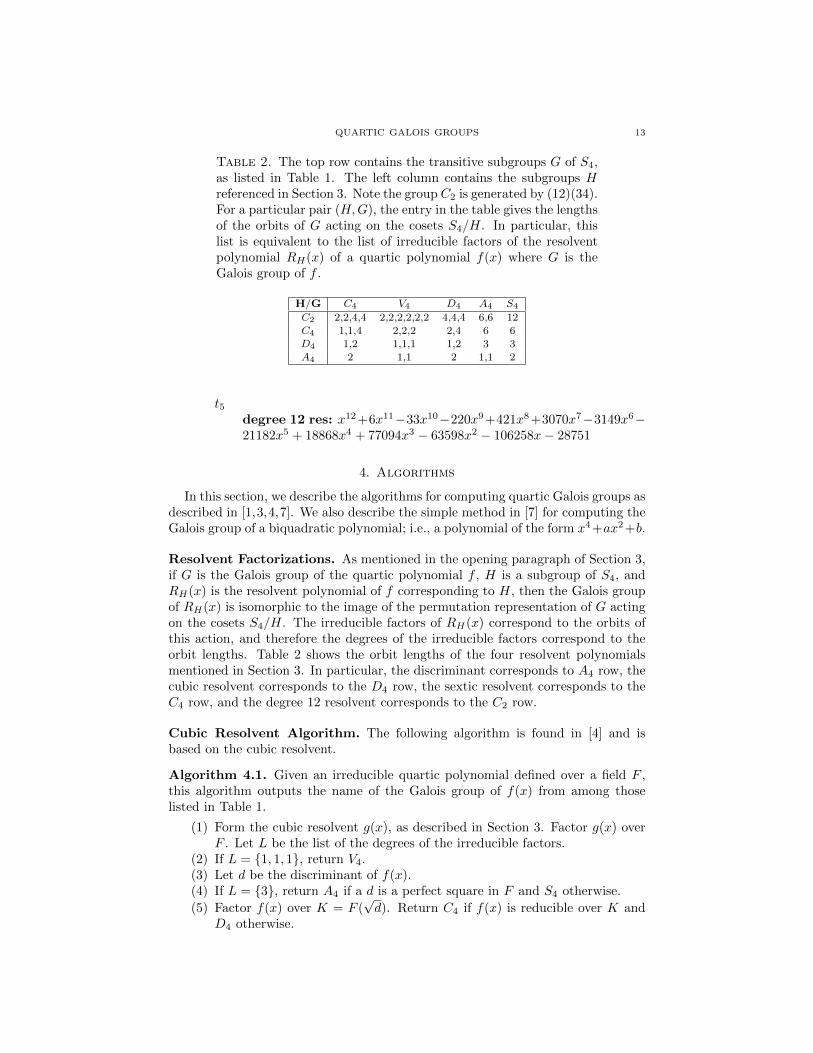
Table 2. The top row contains the transitive subgroups G of S4,as listed in Table 1. The left column contains the subgroups Hreferenced in Section 3. Note the group C2 is generated by (12)(34).For a particular pair (H,G), the entry in the table gives the lengthsof the orbits of G acting on the cosets S4/H. In particular, thislist is equivalent to the list of irreducible factors of the resolventpolynomial RH(x) of a quartic polynomial f(x) where G is theGalois group of f .

H/G C4 V4 D4 A4 S4

C2 2,2,4,4 2,2,2,2,2,2 4,4,4 6,6 12C4 1,1,4 2,2,2 2,4 6 6

D4 1,2 1,1,1 1,2 3 3

A4 2 1,1 2 1,1 2

t5degree 12 res: x12+6x11

�33x10�220x9+421x8+3070x7

�3149x6�

21182x5 + 18868x4 + 77094x3� 63598x2

� 106258x� 28751

4. Algorithms

In this section, we describe the algorithms for computing quartic Galois groups asdescribed in [1,3,4,7]. We also describe the simple method in [7] for computing theGalois group of a biquadratic polynomial; i.e., a polynomial of the form x4+ax2+b.

Resolvent Factorizations. As mentioned in the opening paragraph of Section 3,if G is the Galois group of the quartic polynomial f , H is a subgroup of S4, andRH(x) is the resolvent polynomial of f corresponding to H, then the Galois groupof RH(x) is isomorphic to the image of the permutation representation of G actingon the cosets S4/H. The irreducible factors of RH(x) correspond to the orbits ofthis action, and therefore the degrees of the irreducible factors correspond to theorbit lengths. Table 2 shows the orbit lengths of the four resolvent polynomialsmentioned in Section 3. In particular, the discriminant corresponds to A4 row, thecubic resolvent corresponds to the D4 row, the sextic resolvent corresponds to theC4 row, and the degree 12 resolvent corresponds to the C2 row.

Cubic Resolvent Algorithm. The following algorithm is found in [4] and isbased on the cubic resolvent.

Algorithm 4.1. Given an irreducible quartic polynomial defined over a field F ,this algorithm outputs the name of the Galois group of f(x) from among thoselisted in Table 1.

(1) Form the cubic resolvent g(x), as described in Section 3. Factor g(x) overF . Let L be the list of the degrees of the irreducible factors.

(2) If L = {1, 1, 1}, return V4.(3) Let d be the discriminant of f(x).(4) If L = {3}, return A4 if a d is a perfect square in F and S4 otherwise.(5) Factor f(x) over K = F (

p

d). Return C4 if f(x) is reducible over K andD4 otherwise.


Proof. Steps (2) and (4) follow immediately from Table 2. To prove Step (5),we note that f(x) will be reducible over K = F (

p

d) if and only if K definesa quadratic subfield of f ’s stem field. By the Galois correspondence, quadraticsubfields of f ’s stem field correspond to subgroups H of G of index 2 that containG1, the point stabilizer of 1. On the other hand, the subgroup that corresponds toF (

p

d) is A4 \ G. For the group C4, these two subgroups are the same; namely,{(1), (13)(24)}. For D4, these two groups are di↵erent: A4\D4 = V4 (the transitiveV4), while the subgroup of D4 of index 2 containing the point stabilizer of 1 in D4

is an intransitive V4 = {(1), (13), (24), (13)(24)}. This proves that if G 2 {C4, D4},then f(x) is reducible over K if and only if G = C4. ⇤

We note that [7] contains a modification of Algorithm 4.1. The need to factorf(x) over F (

p

d) is replaced by factoring two additional quadratic polynomials overF ; these two quadratic polynomials make use of the unique simple root of the cubicresolvent. See their paper for complete details.

Sextic Resolvent Algorithm. The following algorithm is found in [3] and isbased on the sextic resolvent.


(1) Form the degree 6 resolvent g(x), as described in Section 3. Factor g(x)over F .

(2) If g is squarefree (that is, if gcd(g(x), g0(x)) = 1), let L be the list of thedegrees of the irreducible factors. Otherwise, replace f by a Tschirnhaustransformation and repeat step 1.

(3) Return C4, V4, or D4 if L = {1, 1, 4}, {2, 2, 2}, or {2, 4}, respectively.(4) Let d be the discriminant of f(x).(5) Return A4 if d is a perfect square in F and S4 otherwise.

Proof. Follows immediately from Table 2. ⇤

Degree 12 Resolvent Algorithm. The following algorithm is found in [1] andis based on the degree 12 resolvent.


(1) Form the degree 12 resolvent g(x), as described in Section 3. Factor g(x)over F .

(2) If g is squarefree (that is, if gcd(g(x), g0(x)) = 1), let L be the list of thedegrees of the irreducible factors. Otherwise, replace f by a Tschirnhaustransformation and repeat step 1.

(3) Return C4, V4, D4, A4, or S4 if L = {2, 2, 4, 4}, {2, 2, 2, 2, 2, 2}, {4, 4, 4},{6, 6}, or {12}, respectively.

Proof. Follows immediately from Table 2. ⇤


Biquadratic Algorithm. The following algorithm is found in [7].

Algorithm 4.4. Given an irreducible biquadratic polynomial f(x) = x4 + ax2 + bdefined over a field F , this algorithm outputs the name of the Galois group of f(x)from among those listed in Table 1.

(1) Let d = 16a4b� 128a2b2 + 256b3.(2) Return V4 if d is a perfect square in F .(3) Let e = a2 � 4b(4) Return C4 if de is a perfect square in F and D4 otherwise.

Proof. Let G be the Galois group of f and K the stem field of f . Clearly, K hasa quadratic subfield, defined by the polynomial g(x) = x2 + ax + b. As noted inthe proof of Algorithm 4.1, the presence of a quadratic subfield is equivalent to theexistence of a subgroup H of G of index 2 that contains G1, the point stabilizer of1. Direct computation shows the groups C4, V4, and D4 have such a subgroup H,while A4 and S4 do not. Therefore G 2 {C4, V4, D4}.

Now d equals the discriminant of f(x) and e is the discriminant of g(x). Ac-cording to Table 2, d is a perfect square if and only if G = V4. This proves Step(2).

Since K is defined by g, K = F (p

e). Note, F (p

d) also defines a quadraticextension of F . As shown in the proof of Algorithm 4.1, F (

p

d) = K if and onlyif G = C4. But F (

p

d) = F (p

e) if and only if de is a perfect square. This provesStep (4). ⇤

5. New Method

In this section, we outline our non-resolvent approach to computing quarticGalois groups. We also show our approach gives rise to an application to biquadraticquartics.

Algorithm 5.1. Given an irreducible quartic polynomial f(x) defined over a fieldF , this algorithm outputs the name of the Galois group of f(x) from among thoselisted in Table 1.

(1) Let K be the stem field f . Factor f over K and let r denote the numberof linear factors.

(2) Return D4 if r = 2.(3) Let d be the discriminant of f(x).(4) If r = 4, return V4 if d is a perfect square in F and C4 otherwise.(5) If r = 1, return A4 if d is a perfect square in F and S4 otherwise.

Proof. Let G be the Galois group of f , K the stem field of f , G1 the point stabilizerof 1 in G, and N the normalizer of G1 in G. By Corollary 2.6, r = [N : G1]. Directcomputation on the groups {C4, V4, D4, A4, S4} shows the corresponding values of[N : G1] are {4, 4, 2, 1, 1}, respectively. The algorithm now follows by combiningthis information with row A4 in Table 2. ⇤

Biquadratic Polynomials. The proof of Algorithm 4.4 shows if f(x) is biquadratic,then the Galois group of f is either C4, V4, or D4. In this section, we show theconverse is true. That is, we show if K is the stem of f(x) where the Galois groupof f is C4, V4, or D4, then there exists a biquadratic polynomial g(x) that definesK. Our proof is constructive.


Algorithm 5.2. Given an irreducible quartic polynomial f(x) defined over a fieldF whose Galois group is either C4, V4, or D4, this algorithm outputs a biquadraticpolynomial defining the same extension as f .

(1) Let K be the stem field f generated by a root r of f . Factor f over K andlet L denote the roots of linear factors; these will necessarily be polynomialsin the variable r of degree 3 (they will be the automorphisms of K/F ).

(2) Pick g(r) 2 L such that g(r) 6= r and g(g(r)) ⌘ r (mod f(r)). So g(r) isan automorphism of order 2.

(3) Let h(x) be the characteristic polynomial of r � g(r). That is, h(x) =Resultantr(x� (r � g(r)), f(r)).

(4) Return h(x) if it is squarefree. Otherwise, replace f by a Tschirnhaustransformation and repeat steps 1–4.

Proof. Let G be the Galois group of f(x), K the stem field of f , and Aut(K) theautomorphism group of K/F . Corollary 2.6 shows Aut(K) is isomorphic to N/G1

where G1 is the point stabilizer of 1 in G and N the normalizer of G1 in G. Theproof of Algorithm 4.4 shows that since G 2 {C4, V4, D4}, K contains a quadraticsubfield. Thus Aut(K) contains a subgroup of order 2, and hence an element oforder 2. This proves Step (2) is possible.

Direct computation shows that if G = V4, there are 3 such choices for g(r). Aspermutations, these automorphisms are given by: (12)(34), (13)(24), (14)(23). Oth-erwise, there is a unique choice for g(r). If G = C4 or D4, g(r) is the permutation(13)(24). Note that these permutations depend on the ordering of the roots of f .Di↵erent orderings will correspond to conjugate permutations. But the cycle typeis invariant under conjugation. So in any case, the permutation g(r) leaves no rootfixed.

Let h(x) = Resultantr(x� (r� g(r)), f(r)). Thus h(x) 2 F [x], and therefore theirreducible factors of h define subfields of K. Suppose the roots of f are a, b, c, d.Suppose further that g(r) permutes the roots in the following way: (ab)(cd). Then

h(x) = (x� (a� b))(x� (b� a))(x� (c� d))(x� (d� c))

= (x2� (a� b)2)(x2

� (c� d)2)

= x4� [(a� b)2 + (c� d)2]x2 + [(a� b)(c� d)]2.

Thus h(x) is biquadratic. If h is irreducible, then since it defines a subfield of K,it must be the case that the stem field of h is exactly K. ⇤

5.1. Example. For example, let f(x) = x4�x3+x2

�x+1. Let K/Q be the stemfield of f . Then factoring f over K shows that K contains all four roots of f . Thefour automorphisms of K are:

r,�r2,�r3 + r2 � r + 1, r3

Direct computation on the 3 nontrivial automorphisms shows that when the 2ndand 4th automorphisms are composed with themselves, they yield the 3rd auto-morphism. When the 3rd automorphism is composed with itself, it yields r. Note,this proves the Galois group of f is C4. Let g(r) = �r3 + r2 � r + 1. Formingthe characteristic polynomial h(x) of r � g(r), we obtain h(x) = x4 + 5x2 + 5, anirreducible biquadratic polynomial.


6. Comparison

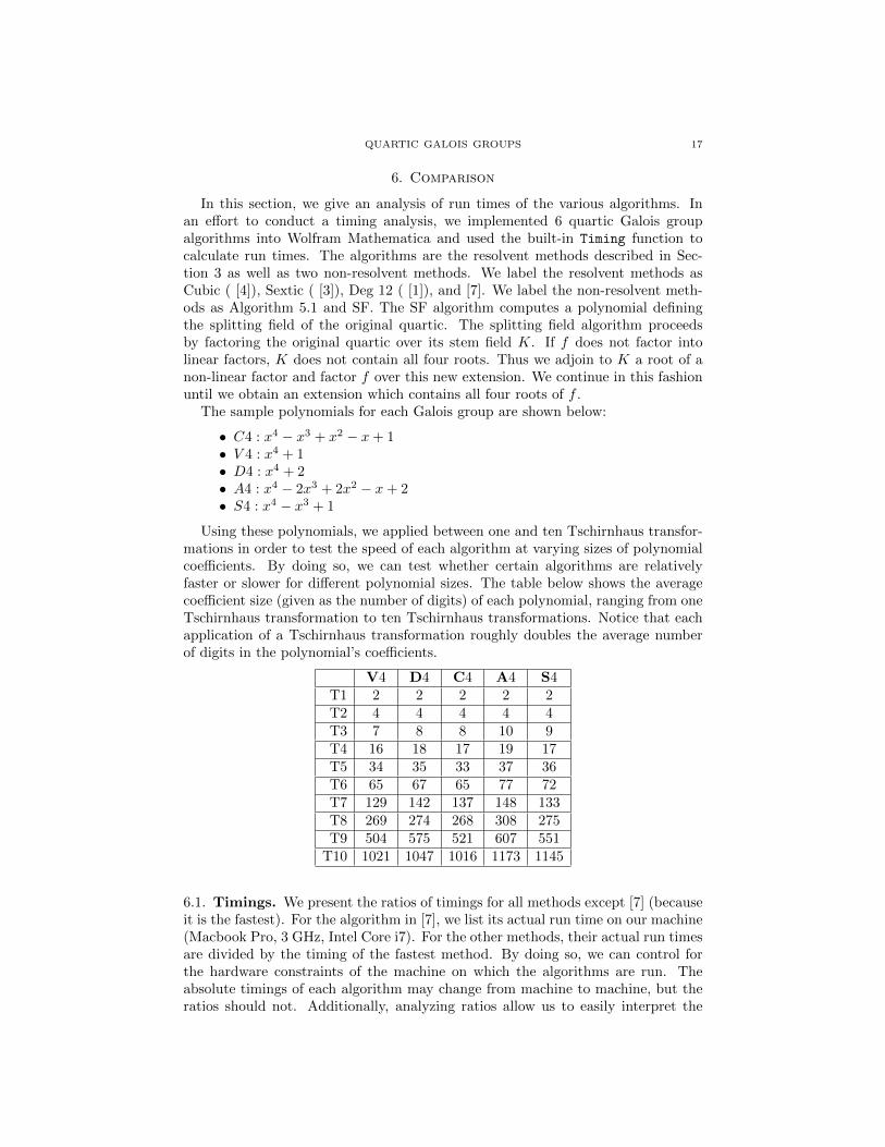
In this section, we give an analysis of run times of the various algorithms. Inan e↵ort to conduct a timing analysis, we implemented 6 quartic Galois groupalgorithms into Wolfram Mathematica and used the built-in Timing function tocalculate run times. The algorithms are the resolvent methods described in Sec-tion 3 as well as two non-resolvent methods. We label the resolvent methods asCubic ( [4]), Sextic ( [3]), Deg 12 ( [1]), and [7]. We label the non-resolvent meth-ods as Algorithm 5.1 and SF. The SF algorithm computes a polynomial definingthe splitting field of the original quartic. The splitting field algorithm proceedsby factoring the original quartic over its stem field K. If f does not factor intolinear factors, K does not contain all four roots. Thus we adjoin to K a root of anon-linear factor and factor f over this new extension. We continue in this fashionuntil we obtain an extension which contains all four roots of f .

The sample polynomials for each Galois group are shown below:

• C4 : x4� x3 + x2

� x+ 1• V 4 : x4 + 1• D4 : x4 + 2• A4 : x4

� 2x3 + 2x2� x+ 2

• S4 : x4� x3 + 1

Using these polynomials, we applied between one and ten Tschirnhaus transfor-mations in order to test the speed of each algorithm at varying sizes of polynomialcoe�cients. By doing so, we can test whether certain algorithms are relativelyfaster or slower for di↵erent polynomial sizes. The table below shows the averagecoe�cient size (given as the number of digits) of each polynomial, ranging from oneTschirnhaus transformation to ten Tschirnhaus transformations. Notice that eachapplication of a Tschirnhaus transformation roughly doubles the average numberof digits in the polynomial’s coe�cients.

V4 D4 C4 A4 S4T1 2 2 2 2 2T2 4 4 4 4 4T3 7 8 8 10 9T4 16 18 17 19 17T5 34 35 33 37 36T6 65 67 65 77 72T7 129 142 137 148 133T8 269 274 268 308 275T9 504 575 521 607 551T10 1021 1047 1016 1173 1145

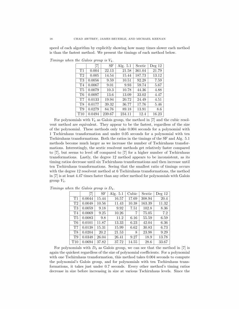
6.1. Timings. We present the ratios of timings for all methods except [7] (becauseit is the fastest). For the algorithm in [7], we list its actual run time on our machine(Macbook Pro, 3 GHz, Intel Core i7). For the other methods, their actual run timesare divided by the timing of the fastest method. By doing so, we can control forthe hardware constraints of the machine on which the algorithms are run. Theabsolute timings of each algorithm may change from machine to machine, but theratios should not. Additionally, analyzing ratios allow us to easily interpret the


speed of each algorithm by explicitly showing how many times slower each methodis than the fastest method. We present the timings of each method below.

Timings when the Galois group is V4.

[7] SF Alg. 5.1 Sextic Deg 12T1 0.004 22.13 21.58 361.04 21.79T2 0.005 14.54 15.44 187.73 13.12T3 0.0056 9.59 10.51 92.28 7.59T4 0.0067 9.01 9.93 59.74 5.67T5 0.0079 10.3 10.78 44.36 4.88T6 0.0097 13.6 13.09 33.02 4.47T7 0.0133 19.94 20.72 24.49 4.51T8 0.0177 39.32 36.77 17.76 5.46T9 0.0279 84.76 89.18 13.91 8.6T10 0.0494 239.67 234.11 12.4 16.23

For polynomials with V4 as Galois group, the method in [7] and the cubic resol-vent method are equivalent. They appear to be the fastest, regardless of the sizeof the polynomial. These methods only take 0.004 seconds for a polynomial with1 Tschirnhaus transformation and under 0.05 seconds for a polynomial with tenTschirnhaus transformations. Both the ratios in the timings of the SF and Alg. 5.1methods become much larger as we increase the number of Tschirnhaus transfor-mations. Interestingly, the sextic resolvent methods get relatively faster comparedto [7], but seems to level o↵ compared to [7] for a higher number of Tschirnhaustransformations. Lastly, the degree 12 method appears to be inconsistent, as itstiming ratios decrease until six Tschirnhaus transformations and then increase untilten Tschirnhaus transformations. Seeing that the smallest ratio of timings occurswith the degree 12 resolvent method at 6 Tschirnhaus transformations, the methodin [7] is at least 4.47 times faster than any other method for polynomials with Galoisgroup V4.

Timings when the Galois group is D4.

[7] SF Alg. 5.1 Cubic Sextic Deg 12T1 0.0044 15.44 16.57 17.69 308.94 20.4T2 0.0048 10.56 11.43 10.38 163.39 11.32T3 0.0059 9.18 9.92 7.51 102.8 8.36T4 0.0069 9.25 10.26 7 75.05 7.2T5 0.0083 9.8 11.2 6.16 55.59 6.59T6 0.0101 11.87 13.33 6.23 42.04 6.36T7 0.0138 15.31 15.99 6.62 30.83 6.73T8 0.0204 20.2 21.53 8 23.98 9.29T9 0.0348 26.04 26.41 9.27 18.9 13.78T10 0.0694 37.82 37.72 14.55 28.6 33.67

For polynomials with D4 as Galois group, we can see that the method in [7] isagain the quickest regardless of the size of polynomial coe�cients. For a polynomialwith one Tschirnhaus transformation, this method takes 0.004 seconds to computethe polynomial’s Galois group, and for polynomials with ten Tschirnhaus trans-formations, it takes just under 0.7 seconds. Every other method’s timing ratiosdecrease in size before increasing in size at various Tschirnhaus levels. Since the


minimum timing ratio is the cubic method at five Tschirnhaus transformations, wecan conclude that the method in [7] is at least 6.16 times faster than any othermethod for polynomials with Galois group D4.

Timings when the Galois group is C4.

[7] SF Alg. 5.1 Cubic Sextic Deg 12T1 0.0048 16.19 15.32 19.37 255.32 17.23T2 0.0055 10.06 9.56 10.72 140.06 10.17T3 0.0065 8.4 8.26 7.42 84.47 7.42T4 0.0074 8.3 8 5.83 58.63 5.74T5 0.0089 8.9 8.67 5.36 45.16 5.26T6 0.0112 10.67 10.29 5.27 34.43 5.03T7 0.0146 13.65 12.8 5.55 25.21 5.04T8 0.0216 17.93 16.82 6.13 18.45 5.72T9 0.0343 23.21 21.58 7.02 12.72 8.01T10 0.0703 32.49 32.77 9.37 10.05 15.27

Again, we see that the method in [7] is the fastest method for quartic polyno-mials with Galois group C4. This method takes 0.0048 seconds for polynomialswith one Tschirnhaus transformation and 0.0703 seconds for polynomials with tenTschirnhaus transformations. The timing ratios of all methods except the sexticresolvent method become smaller before becoming larger compared to [7] as we in-crease the size of the polynomial coe�cients. The sextic resolvent method becomesrelatively faster as we increase coe�cient size. We can say that the method in [7]is at least 5 times faster than any other method for polynomials with Galois groupC4, as the smallest ratio is 5.03. This occurs when we use the degree 12 method onpolynomials with six Tschirnhaus transformations.

Timings when the Galois group is A4.

[7] SF Alg. 5.1 Sextic Deg 12T1 0.004 233.39 17.82 325.28 22.25T2 0.0045 198.96 13.17 175.58 14.01T3 0.0055 186.3 10.41 97.92 9.8T4 0.0065 245.72 10.05 65.04 8.83T5 0.0077 463.4 11.97 47.33 10.13T6 0.0094 1026.79 16.11 36.55 14.47T7 0.0124 3305.62 24.37 28.47 28.25T8 0.0178 9043.24 44.08 21.43 71.57

For quartic polynomials with Galois group A4, the method in [7] and the cu-bic resolvent method are equivalent, and they are the fastest. We only used eightTschirnhaus transformations for polynomials with this Galois group due to com-putational constraints of our machine. The ratios of the SF, Alg. 5.1, the degree12 methods decrease in size initially, and then increase in size as we increase thesize of polynomial coe�cients. On the other hand, the sextic resolvent methodbecomes relatively faster as we increase the size of coe�cients, when comparedto [7]. This method is at least 47% faster than any other method, given a randomquartic polynomial with Galois group A4, as the smallest ratio is 1.47, occurringwhen we apply the cubic resolvent method to a polynomial with eight Tschirnhaustransformations.


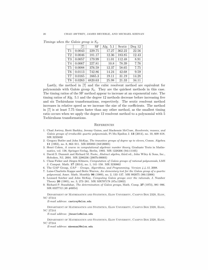
Timings when the Galois group is S4.

[7] SF Alg. 5.1 Sextic Deg 12T1 0.0043 229.75 17.27 362.22 22.56T2 0.0046 181.17 12.36 183.85 12.43T3 0.0057 179.99 11.01 112.48 8.91T4 0.0067 227.81 10.8 78.39 7.76T5 0.0088 376.59 12.37 58.65 7.75T6 0.0113 742.86 14.24 42.68 9.59T7 0.0165 1665.3 19.11 31.19 14.28T8 0.0263 4820.63 25.98 21.33 34.11

Lastly, the method in [7] and the cubic resolvent method are equivalent forpolynomials with Galois group S4. They are the quickest methods in this case.The timing ratios of the SF method appear to increase at an exponential rate. Thetiming ratios of Alg. 5.1 and the degree 12 methods decrease before increasing fiveand six Tschirnhaus transformations, respectively. The sextic resolvent methodincreases in relative speed as we increase the size of the coe�cients. The methodin [7] is at least 7.75 times faster than any other method, as the smallest timingratio occurs when we apply the degree 12 resolvent method to a polynomial with 5Tschirnhaus transformations.

References

1. Chad Awtrey, Brett Barkley, Jeremy Guinn, and Mackenzie McCraw, Resolvents, masses, and

Galois groups of irreducible quartic polynomials, Pi Mu Epsilon J. 13 (2014), no. 10, 609–618.MR 3235830

2. Gregory Butler and John McKay, The transitive groups of degree up to eleven, Comm. Algebra

11 (1983), no. 8, 863–911. MR 695893 (84f:20005)3. Henri Cohen, A course in computational algebraic number theory, Graduate Texts in Mathe-

matics, vol. 138, Springer-Verlag, Berlin, 1993. MR 1228206 (94i:11105)

4. David S. Dummit and Richard M. Foote, Abstract algebra, third ed., John Wiley & Sons, Inc.,Hoboken, NJ, 2004. MR 2286236 (2007h:00003)

5. Claus Fieker and Jurgen Kluners, Computation of Galois groups of rational polynomials, LMS

J. Comput. Math. 17 (2014), no. 1, 141–158. MR 32308626. The GAP Group, GAP – Groups, Algorithms, and Programming, Version 4.4.12, 2008.7. Luise-Charlotte Kappe and Bette Warren, An elementary test for the Galois group of a quartic

polynomial, Amer. Math. Monthly 96 (1989), no. 2, 133–137. MR 992075 (90i:12006)8. Leonard Soicher and John McKay, Computing Galois groups over the rationals, J. Number

Theory 20 (1985), no. 3, 273–281. MR MR797178 (87a:12002)

9. Richard P. Stauduhar, The determination of Galois groups, Math. Comp. 27 (1973), 981–996.MR 0327712 (48 #6054)

Department of Mathematics and Statistics, Elon University, Campus Box 2320, Elon,

NC 27244E-mail address: [email protected]

Department of Mathematics and Statistics, Elon University, Campus Box 2320, Elon,

NC 27244E-mail address: [email protected]

Department of Mathematics and Statistics, Elon University, Campus Box 2320, Elon,NC 27244

E-mail address: [email protected]

algorithms for computing quartic galois groups over …facstaff.elon.edu/cawtrey/abk-quartic.pdf ·...

Documents