algorithms for generalized mean variance problems
DESCRIPTION
Algorithms for generalized mean/variance problemsTRANSCRIPT
1
Introduction
The principles of portfolio theory were laid more than 40 years ago. But although it was
designed for managing private and institutional portfolios of financial assets, among the largest
banks in the world there are few which systematically apply the perceptions of portfolio theory.
And even if applications are implemented, there is only a small number of market participants
who are able to utilize more than the basics. There are only a few, typically rather small,
investment banks and institutional investors in the world who have the human resources
available to exploit the superior theoretical concepts for the real investment process. However,
they tend not to make their knowledge publicly available.
The realization of portfolio theory and its modern developments in downside risk management
necessitates the use of powerful computers and software programs. Although the theoretical
work has advanced considerably, neither in the research nor in practice has there been
sufficient work to provide programmable algorithms which would make approaches
understandable and applicable. This thesis is intended to show how abstract theories can be
applied to real portfolio management using modern financial instruments. Its purpose is to help
practitioners to implement portfolio strategies based on theoretical concepts. It summarizes
existing theories and expands them to frameworks which are designed to generate specific
asset allocation decisions.
In the first chapter the basics of portfolio theory are summarized. It follows the description of
quadratic optimization algorithms. They are needed to implement and solve mean/variance
optimization problems respecting various restrictions resulting from investor preferences or
from laws. Mean/variance principles are the basis for asset allocation decisions and although
they are extended and alternative approaches are given in this thesis, all investment decision
criteria observe them. Markowitz [1987] provided a book which contains the principles of the
mean/variance approach where linear restrictions are imposed. Nevertheless, this thesis extends
the basic rules of Markowitz and gives comprehensive numerical examples.
The second chapter is concerned with international asset allocation decisions. Investment
decisions arising from international diversified portfolios are typically more complex than
merely domestic investments, since they require one to respect currency movements
supplementary to asset price movements. Due to the development of advanced markets for
currency derivatives the currency allocation decision may be influenced by hedging decisions:
selling short forward contracts on currencies provides opportunities for lowering the impact of
the currency risk. Since the hedge ratio may be chosen in accordance with the expected
currency development, hedging of the currency exposure can be done without avoiding
potential gains on currencies. Traditionally, the hedging and the asset allocation decision are
done subsequently. This is done with respect to the fact that currency and asset returns are
2
related to each other. Thus, it is reasonable to take the currency and the asset allocation
decision simultaneously. The approach introduced in chapter two simultaneously optimizes the
hedge ratios and the fractions invested in different countries. Since in contrast to the traditional
international asset allocation decisions it elaborates a model where variable hedging
opportunities are allowed, it is called a variable hedging model. Apart from the analytical
presentation of the model, chapter two contains a case study for an investor with the reference
currency US-$ who diversifies internationally.
Chapter three discusses downside risk measures. A major disadvantage of mean/variance
problems is the consideration of symmetrical payoff patterns. That is, oscillations to the upside
of returns series are interpreted as disadvantageous occurrences as well as downside
oscillations. Obviously, investors are more concerned with the downside movements than with
the upside potential. Therefore, downside risk approaches exclusively accept downside
oscillations as relevant measures of risk. Although these approaches were already developed at
the beginning of the fifties, they succeeded in the mid seventies with the introduction of lower
partial moment frameworks. A special case of lower partial moments is the safety first
principle. This allows investors to find out portfolios revealing a minimum probability for
falling short of specified return level. Chapter three contains a discussion of the literature
concerning lower partial moments and the safety first principle and applies it to investment
allocation decisions. For identifying minimum shortfall probability when the investment
opportunity set is restricted, the results from chapter one are used. It is shown that one of the
major advantages of the Markowitz algorithm compared to other methods which minimize
quadratic functions, is that it is easily applicable to investment problems based on the
mean/variance principle.
The last chapter investigates downside risk problems when derivatives, such as options, are
used to influence the probability distributions of the payoffs. Using options to protect
portfolios against pitfalls is a widely used technique. However, it is not clear how using options
influences the probability distributions of the returns. In chapter four, a simulation approach is
shown which allows their comparison. Applying downside risk measures allows comparing
them.
Apart from those who are interested in applied portfolio theory, this thesis is designed for
programmers. Therefore, this work is accompanied by a software program which contains all
the algorithms described. The figures and numerical examples contained in the following
chapters are mostly calculated by this program.
3
Chapter IAlgorithms for generalized mean/variance problems
This chapter lays the foundations for this thesis. In the first section the fundamentals of
portfolio theory are summarized. These are well known from the standard literature (see for
instance Ingersoll [1987] and Huang and Litzenberger [1988]). Since readers with different
knowledges of portfolio theory are addressed by this thesis, this section is to provide the reader
with the most important equations and interpretations of standard portfolio theory. In section
one, the main results of portfolio theory without respecting practical investment restrictions are
pointed out.
Since with this thesis people are addressed who are concerned with the implementation of
investment strategies, in the subsequent sections portfolio problems subject to investment
restrictions are investigated. The algorithms provided in the sections two, three, and four are
based on the critical line algorithm introduced by Markowitz [1956 and 1987] which is
therefore sometimes referred to as Markowitz algorithm. Section two deals with the ordinary
form of the algorithm. This allows solving portfolio problems subject to equality restrictions
and with the exclusion of short selling. However, in the real investment process it is not
sufficient to impose purely equality restrictions. Typically, investment situations are
characterized by lower or upper boundaries for the fractions invested in specific asset classes
or in combinations of asset classes. For instance, investors may be prepared to invest in foreign
stocks but not more than fifty percent of the investment capital. This restriction will require to
impose a "smaller than" restriction for foreign stocks. Although these problems are briefly
discussed in Markowitz's [1987] book, they are not explicitly solved. Therefore section three
deals with an algorithm which allows imposing linear inequality and equality restrictions. This
is, in addition to equality restrictions, "smaller than" and "greater than" restrictions are added.
Short sales remain excluded. Since this generalizes the ordinary form of the Markowitz
algorithm this is called generalized Markowitz algorithm.
Some investment situations might require the exclusion of short sales for specific asset classes
but not for others. Although the generalized critical line algorithm allows to solve very general
investment problems the lowest fraction for each asset in the portfolio is zero: no asset can be
sold short. Permitting negative portfolio fractions provides the opportunity to sell short some
assets of the portfolio. Variables which are unrestricted to the downside are called
unrestricted-in-sign variables. In the fourth section this problem is investigated: an algorithm is
provided which allows the solution of investment problems with unrestricted-in-sign variables
and with equality and inequality restrictions. Since this algorithm is not discussed in the

4
literature provided by Markowitz but since it is nevertheless based on the critical line algorithm
this is called extended Markowitz algorithm.
All variants of the Markowitz algorithm are completed by comprehensive numerical examples.
This shall enable the reader to exactly understand the algorithms in order to allow
programming them. Since this chapter provides the methodical basics for solving general
mean/variance problems, case studies with practical impact are not provided here but in the
following chapters. To facilitate the understanding of the principles of the algorithm, the
applications in this chapter deal with a hypothetical three asset case.
1. Fundamentals of Portfolio Theory
Harry Markowitz [1952][1959] laid the foundations for a new view of investments in financial
assets. He showed that the fundamental issue of capital investment should no longer be to pick
out dominant stocks but to diversify the wealth among many different assets. His work marked
a turning point in the academic literature concerning capital investments, because he showed
that the success of investment does not purely depend on return, but also on the risk which has
to be taken. Furthermore, he showed that the risk of investments is influenced by the
correlations between different assets. Thus, the objective of investors can no longer be seen in
maximizing the "performance"1 only. The performance strategies must be evaluated in the
context of a certain level of risk. Investors are faced with complex optimization problems, the
solution of these problems leads to a specific investment strategy, i.e. a concrete portfolio of
assets. The optimization process is referred to as portfolio selection.
That diversification is a crucial issue of investment, and that risk has to be considered in
addition to portfolio returns, is an intuitive investment issue rather than a highly academic
perception. So the main results of Markowitz' work have to be seen in his answering the
question how to measure investment "performances" and investment risks. The answers to
these questions were derived from very general assumptions of utility theory. Markowitz
presented "investment rules" which maximize the expected utility of investors.
The first section of this thesis summarizes briefly the main results of portfolio theory. In the
first part, the mean/variance principle is elaborated from the standard assumption of utility
theory. The following part contains a short survey of the analytical basics of the mean/variance
1 The term "performance" should be interpreted in its original sense, rather than according to the newer
literature of portfolio performance, where it is referred to as risk adjusted portfolio returns.

5
efficient set and, in conclusion, it is shown that under certain assumptions the single period
optimization problem is equivalent to a multiperiod, discrete time portfolio selection model.
1.1. Utility theory and mean/variance principle
The aim of this section is to show, how the "performance" and risk of any portfolio can be
measured. It was assumed by von Neumann/Morgenstern [1953] that rational investors behave
according to five fundamental axioms of rationality. They showed that this assumption is
consistent with maximizing expected utility, given a fixed bundle of consumption goods and
investment opportunities. The respective utility function has to be twice differentiable,
increasing and strictly concave (see Ingersoll [1987], pp. 21-22). Thus, every rational investor
endeavours to maximize his individual expected utility of consumption. First, a single period
case of portfolio optimization is considered. Since in this case end-of-period-wealth equals
consumption, it is admissible to maximize expected utility of end-of-period wealth instead ofconsumption. Let %Wt +1 denote the end of period wealth of a representative investor and U his
(her) (twice differentiable, increasing and strictly concave) utility function. Then the investors'optimization problem can be stated as follows (see Huang/Litzenberger [1988], pp. 60-61):
(1.1) ( )max~
EU Wt +1
( )U Wt~
+1 may be expressed as ( )U EW W EWt t t~ ~ ~
+ + ++ −1 1 1 , where E denotes the expectations
operator. Since a single period model is considered, the time sub-index is dropped from now
on. Applying a Taylor series expansion leads to:
( ) ( ) ( )( ) ( )( ) ( )( )U W U EW U EW W EW U EW W EWi
U EW W EWi
ii~ ~ ~ ~ ~ ~ ~ ~
!
~ ~ ~( )= + ′ − + ′′ − + −=
∞
∑12
12
3
U i( ) is the i-th derivative of the utility function U with respect to the term in brackets. It is
assumed to be at least twice differentiable. Substituting the above expression into equation(1.1) renders a restatement, where σW
2 denotes the variance of wealth:
(1.2) ( ) ( ) ( ) ( ) ( ) ( )EU W U EW U EW E W EW U EWi
U EW mWi
ii
~ ~ ~ ~ ~ ~
!
~( )= + ′ − + ′′ +=
∞
∑12
12
3
σ
6
mi represents the i-th moment of the probability distribution of %W . Equation (1.2) highlights
the fact that the expected utility of wealth depends on the expected end of period wealth and
its variance. Without making any assumptions about the probability distribution, the expected
utility of wealth is furthermore influenced by the higher moments. If on the other hand it is
assumed that the end of period wealth %W is normally distributed, then the moments of order
greater than two can be stated as functions of the expected end of period wealth and its
variance. This allows reformulating (1.2) as:
(1.3) ( ) ( ) ( ) ( ) ( )EU W U EW U EW E W EW U EW W~ ~ ~ ~ ~ ~
= + ′ − + ′′12
2σ
(1.3) indicates, that investors have to concern themselves merely with the mean and the
variance of the end of period wealth for normal probability distributions. It should be
emphasized that equation (1.2) holds for any probability distribution whereas the
mean/variance principle can be deduced out of (1.3): The higher the expected utility of wealth
given a constant level of variance, the higher the expected level of end of period wealth will be.
If EW% is held constant, the variance of the end of period wealth has to be minimized to
maximize the expected utility. Thus, the "performance" of any portfolio according to von
Neumann/Morgenstern's utility theory is measured as the expected end of period wealth
assessed by a portfolio of assets. The portfolio's risk is measured by the variance of the end of
period wealth. This is called a mean/variance principle of portfolio diversification.
If a normal distribution for the end of period wealth cannot be assumed, the mean/variance
principle can be rescued for arbitrary wealth distributions, if quadratic utility functions of the
form ( )U W Wb
W~ ~ ~= −
22 are imputed. In this case all moments of order greater than two are
zero and can thus be dropped. Substituting the utility function into equation (1.2) the new
objective function may be expressed as:
(1.4) ( ) ( ) ( ) ( ) ( )EU W E Wb
EW E Wb
E EW W~ ~ ~ ~ ~
= − = − +
2 2
2 2 2σ
Just as in equation (1.3) equation (1.4) shows that investors endeavour to minimize the
variance of wealth for a given level of expected end of period wealth. Two alternative
assumptions can be made to deduce the mean/variance principle out of utility theory:
1. The end of period wealth is distributed normally , or
2. investors are faced with quadratic utility functions.
7
1.2. Mean/variance efficient frontier
From the results of the last section it can be established that expected utility maximizers
minimize the variance of the end of period wealth subject to a given level of expected end of
period wealth. This is equivalent to minimizing the variance σ2 of returns of a portfolio where
the expected portfolio return E is fixed. Analytically this can be stated as:
(1.5)
min min '
. . : '
'
ω ωσ ω ω
ω µω
2
1
=
==
V
s t E
e
If n portfolio assets are being considered, then ω ∈ℜn represents the vector of portfolio
weights, V nxn∈ℜ represents the variance-covariance matrix of portfolio returns, µ ∈ℜn the
vector of expected returns, and e n∈ℜ the unity vector. The first constraint secures that the
expected portfolio return equals E and the second one enforces the portfolio weights to sum
up to unity. Merton [1972] showed, that the solution of problem (1.5) can be characterized by
the following function2:
(1.6) σ = − +122
dcE bE a( )
σ represents the standard deviation of portfolio returns; a,b,c, and d are real constants which
are defined as follows:
(1.7) a≡ −µ µ' V 1 b≡ −µ' V e1 c≡ −e V e' 1 d≡ −ac b 2
Huang/Litzenberger [1988] (p.66) show, that equation (1.6) represents a hyperbola. Since it
describes efficient portfolios, i.e. portfolios with minimum risk for any given level of expected
return, the graph of function (1.6) is called efficient frontier, which is a well known result from
2 Although this was already shown by Roy [1952] the most well known reference for the following equation is
Merton [1972]. In chapter three the Roy's [1952] paper will be discussed in detail.

8
portfolio theory. The aim of this section is to summarize some analytical properties of the
efficient frontier. The formulae are presented without proof, the interested reader may for
instance refer to Huang/Litzenberger [1988] (chapter 3).
The vector of portfolio weights for any efficient portfolio can be calculated as
(1.8) ω µ µµ
= − + − = − − −− − − −V
dc be E
V
dae b
V
dcE b
V e
dbE a
1 1 1 1
( ) ( ) ( ) ( )
where first equation shows that the portfolio fraction invested in one of the n assets is a linear
function of the portfolio's expected return. The second equation shows, that each efficient
portfolio can be expressed as a function of two portfolios: V −1µ and V e−1 . In equation (1.9) it
is shown that the latter portfolio is the minimum variance portfolio. It is the portfolio withlowest possible variance given n portfolio assets. It will be characterized by variance σmvp
2 ,
expected return E mvp , and vector of portfolio weights ω mvp . They can be calculated as:
(1.9) Eb
cmvp = σmvp c2 1
= ω mvpV e
e V e cV e= =
−
−−
1
111
'
Any two efficient portfolios p and q have covariance
(1.10) σ pq p qc
dE
b
cE
b
c c= −
−
+1
,
which determines the covariance between the minimum variance portfolio with any efficient
portfolio p as:
(1.11) σ σp mvp mvpc, = =1 2
Each hyperbola may be characterized by asymptotes; in case of the efficient frontier they are
identified for large σ by:
(1.12) Eb
c
d
c= ± σ
9
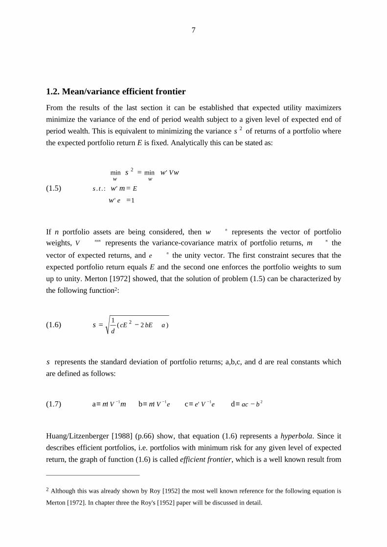
Figure 1.1. depicts the graph of an arbitrary efficient frontier and its asymptotes.
standard deviation
expe
cted
ret
urn
Figure 1.1: Efficient Frontier and its asymptotes
The equations above briefly summarize the main results of the classical portfolio theory and lay
the foundation for the more advanced applications in the following chapters. So far, it has been
assumed that investments are possible only in risky assets. If the investment opportunity set is
extended by a riskless asset, i.e. an asset with zero variance, the well established CAPM (see
Sharpe [1964], Lintner [1965], and Mossin [1966]) equilibrium equation can be derived, where
the expected return on any portfolio depends linearly on the return on the market portfolio:
(1.13) E r E rm− = −β( )
The notation in equation (1.13) is as follows: r represents the riskless return, β the beta of the
portfolio against the market and Em the expected return on the market portfolio. Black [1972]
showed that the assumption of the existence of a riskless asset is unnecessary if instead of the
riskless asset a portfolio is used, which elucidates zero covariance with the returns on the
market portfolio and has a zero beta. It can easily be shown that a zero beta portfolio exists,
whenever the market portfolio is an efficient risky portfolio (see e.g. Huang/Litzenberger
[1988]). The Black form of the CAPM is called zero-beta CAPM. Let E z denote the expected
return on the zero-beta portfolio, then (1.13) may be modified to:
10
(1.14) E E E Ez m z− = −β ( )
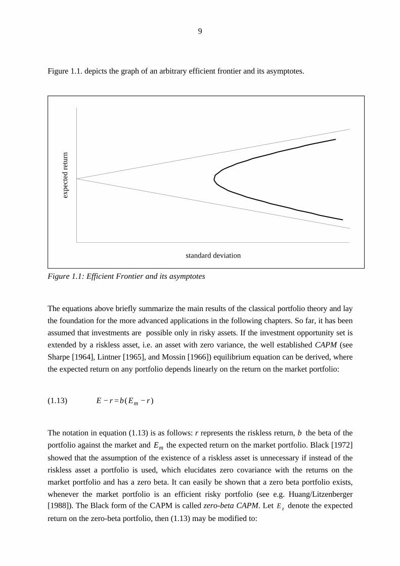
Thus a linear efficient frontier is developed in the case of the existence of a riskless asset or a
zero-beta portfolio. It may be shown that it is tangent to exactly one point of the "risky-assets
efficient frontier", which is the market portfolio. The tangency is generally called Capital
Market Line (CML). Figure 1.2 illustrates this phenomenon:
standard deviation
expe
cted
ret
urn
Market portfolio
Figure 1.2: Efficient Frontier and Capital Market Line
Figure 1.2. clearly illustrates that the market portfolio is the only efficient risky portfolio in the
case of the existence of a riskless portfolio. Given the riskless rate of interest r (or the expected
return on the zero-beta portfolio Ez) the expected return on the market portfolio can be
calculated as:
(1.15) Ea br
b crm =−−
The portfolio fractions are received by substituting (1.15) into (1.8)
11
(1.16) ( )( )ωµ
µµm
V re
e V re b crV re= −
−=
−−
−
−−
1
111( )
' ( ),
where the portfolio fractions sum up to unity. If a riskless asset exists, portfolio (1.16)
represents the only risky optimal portfolio, i.e. the only risky portfolio which is chosen by
investors maximizing the expected utility within a single period.
1.3. Discrete time intertemporal portfolio theory
The considerations so far assumed an investor whose relevant time horizon is a single period.
Of course this is not an appropriate characterization of the real decision situation of investors.
This section will deal with a maximizer of expected utility in an multi-period frame. To begin
with, no more is assumed than an additively separable utility function. Since the wealth at the
end of all consideration periods depends on the consumption plan in the preceding periods, his
utility function is assumed to be ( )U C C C WT T0 1, ,..., ,~
, where C represents the consumption
in the respective period and T the end period of investor's life. Then the objective function of
the considered investor according to the previous section may be expressed by3:
(1.17) ( )[ ] ( )max , , ...,,C
t T tt
E U C C C J Wω
0 1 ≡
By exploiting the fact that U is additively separable, and assuming that the bequest in period T
is denoted by ( )B WT~
, (1.17) may be expressed as:
(1.18) ( ) ( ) ( )J W E U C B WtC
t Tt
T
t
= +
=
∑max~
,ωτ
τ=
= ( ) ( ) ( )max max~
, ,Ct t
Ct t T
t t
T
t t t
E U C E U C B Wω ω
ττ
+ +
+
+=∑
∆∆
∆
3 For an overview see Ingersoll [1987] pp. 235-250, the original reference is Samuelson [1969]. The
intertemporal portfolio problem in a continuous time case was treated by Merton [1969] in the same issue of the
Review of Economics and Statistics as Samuelson's paper.
12
( ) ( )= + +U C E J Wt t t t~
∆ ( ) ( )= + +U C E J W Wt t t ∆~
∆ %W represents the change in wealth between period t and t t+ ∆ . ∆t is assumed to be a very
short time interval. Applying a Taylor series expansion provides:
(1.19) ( ) ( ) ( )01
22= + + +
U C E J W W J W W o tt t t t'~
' '~
( )∆ ∆ ∆
The term ( )o t∆ summarizes the terms dependent on ∆t of an order higher than two; they are
approximately zero if ∆t is assumed to be an extremely short time interval. Then an
assumption about the changes in wealth is added. In the following part of this section ∆ %W
W is
presumed to be distributed normally, i.e. follows an arithmetic Wiener process4. Let ~zW
denote a standard normal distributed random variable, µW the expected relative change in
wealth, σ W2 its variance, and Yt the income in period t, for the relative changes in wealth
holds:
(1.20)∆ ∆ ∆
%%
W
Wt z tW W W≡ +µ σ
( )µ ω ω µ ω µ
σ ω ω
Wt t
t
t t
t
W
e rC Y
Wre r
C Y
W
V
≡ − + −−
= − + −−
≡
1
2
' ' ' ( )
'
The definition of µW ensures that the sum of the fractions of the riskless and the risky assets
equal unity. Substituting (1.19) into (1.20) and rearranging yields:
(1.21) ( ) ( ) ( ) ( )G W C U C W J W re rC Y
Wt W J W V tt t t t t
t t
tt t, ' ' ( ) ' ' '≡ + − + −
+
+ω µ ω ω∆ ∆1
22
Differentiating G with respect to ω provides the following multi-period portfolio of expected
utility maximization:
4 Stochastic processes were first introduced by Bachelier [1990] into the theory of capital markets.
13
(1.22)( )
( )ω µ= − −−J W
W J WV ret
t t
'
' '( )1
Since the fraction of wealth 1 − ω' e is invested in the riskless assets (lending if 1 − ω' e >0 and
borrowing if 1 − ω' e <0) the optimum risky portfolio may be normalized to:
(1.23)( )( )
ωµ
µ=
−
−
−
−V re
e V re
1
1'
Comparing portfolio (1.22) to (1.16) proves that the holdings of the multi-period optimum
portfolio are proportional to the holdings of the single period optimum portfolio. The solution
of the multi-period problem (1.17) can also be obtained by solving the single period problem.
Thus, in the present simple form of the multiperiod portfolio selection model, one can
equivalently use a single period model. An important assumption of this model is, that the
parameters of the underlying Wiener process (1.20) remain constant over time. If thisassumption is given up, i.e. if it is assumed that µW and σW
2 are dependent on a set of state
variables, then the relative changes in wealth follow a more general diffusion process instead of
a Wiener process and the continuous time version of the CAPM (see Merton [1973]) has to be
applied. An important result proven by this study is that for each state variable a single hedge
portfolio has to be used. This guarantees protection against different sources of risk which are
established by the state variables. The major property of the hedge portfolios are that they
produce maximum correlation with the respective state variable. The object of this thesis is to
provide algorithms for the portfolio optimization process and not the investigation of
continuous time models. In this chapter attempts have been made to capture optimization
solutions for the single period model, which also hold for the simple case of a discrete time
multi-period model.
The standard portfolio selection model of Markowitz starts with the assumption that no
riskless asset is available. Thus, the multi-period optimum portfolio is considered excluding
riskless assets. This is then compared to the single period optimum portfolio. In this case figure
(1.17) has to be maximized subject to e ' ω = 1 , since it is not possible to implicitly construct
this requirement as in (1.20). Let λ denote the Lagrange multiplier belonging to the constraint
e ' ω = 1 , then the optimum condition (1.22) may be restated in the new context as (see
Ingersoll [1987], p. 288):
14
(1.24)( )
( ) ( )ω µ
λ= − −− −J W
W J WV
W J WV et
t t t t
'
' ' ' '1 1
Equation (1.24) points out that the intertemporal discrete-time optimum portfolio equivalent to
the single period optimum portfolio in (1.8) consists of two portfolios: V −1µ and V e−1 known
as the minimum variance portfolio. Thus, even when the investment opportunity set is limited
to purely risky assets, the single period and the multi-period problem are solved by the same
portfolio. No matter which problem is to be solved, the optimum portfolio maximizes both: the
one period expected utility function (1.1) and the multiperiod expected utility function (1.17).
This holds as long as the investment opportunity set is constant over time, i.e. the underlying
processes are Wiener processes rather than generalized diffusion processes. Although in a
discrete time intertemporal portfolio optimization framework the sum of the expected utilities
of periodical consumption is maximized, without assuming intertemporal changes in µW and
σW the solution of the single period problem does not differ from that of the multi-period
problem. Consequently, the following sections will assume a one period problem. Its solution
also solves the multi-period model for constant decision variables.
2. The ordinary Markowitz-algorithm
The ordinary Markowitz algorithm is concerned with the solution of quadratic programs
subject to equality and non-negativity restrictions. Extensions of it are given in the following
sections. In addition to equality restrictions, the generalized Markowitz algorithm solves
quadratic problems subject to arbitrary inequality restrictions. Unrestricted-in-sign variables are
furthermore imposed to the extended Markowitz algorithm.
In section one of the first chapter the fundamentals of portfolio theory were considered. The
purpose of that section was to introduce the reader who may not be very familiar with
portfolio theory to the main topic of this thesis. Although Markowitz's theory [1952]
introduced a revolutionary understanding of capital investment at that time, it does not exactly
reconstruct the decision situation of investors. A major problem which might occur is that the
optimal investment policy recommended by (1.8), (1.16), (1.21), or (1.24) cannot be
transposed into reality due to legal restrictions or the investment philosophy or other reasons
due to the investor's attitudes. Specifically, restrictions may be imposed on some of the
available assets, the vector of portfolio weights ω is restricted. Typically, one of the most
common requirements to any investment policy is to exclude short sales, that is to prohibit
negative portfolio fractions of one or more portfolio assets. Although in the theory the
inclusion of such restrictions into equation (1.5) is not a problem, the difficulty lies in the
15
practical implementation. A simple Lagrange approach as in (1.5) and (1.6) will not be
sufficient to find a solution. The problem has to be solved by a quadratic program. General
algorithms may be found in standard operations research literature, e.g. in Winston [1991] (pp.
658-665). Since these algorithms are not specifically fitted to the mean/variance problem, the
computational efficiency can be increased by using an algorithm developed by Markowitz
[1956]. Although it is not exclusively employable for solutions of the mean/variance problem,
it was constructed paying special attention to such problems. The topic of the following
section is the Markowitz algorithm where short selling restrictions are imposed. Since the
structure of such restrictions is rather simple, this variant will be labelled ordinary Markowitz
algorithm. Most aspects of his subject were covered in detail in Markowitz's book [1987].
Consequently, there is no reason to prove the respective equations. However, this section
provides extensions of the original algorithm in some aspects: in part three a special case is
investigated and in part five it is shown that the restricted efficient frontier, in contrast to the
unrestricted efficient frontier discussed earlier, is not differentiable. Apart from short sales
restrictions, the ordinary Markowitz algorithm merely includes equality restrictions. Extensions
of this approach, which are not covered by Markowitz's book, will be developed in subsequent
sections. A simplification of the model is to be found in Markowitz/Schaible/Ziemba [1992]
where the mean/variance problem for lognormal markets and power utility functions is solved
subject to arbitrary restrictions. Since this makes it more specific, this thesis concentrates on
the original algorithm.
The purpose of this section is to show how the Markowitz algorithm works and how it may be
applied to mean/variance problems. It is subdivided in the following parts. Part one states the
general model and the Lagrangian. Part two derives the Kuhn-Tucker conditions for the
problem and summarizes the optimum conditions. A special case is considered in part three.
The following two parts investigate whether the efficient frontier is continuous and
differentiable when short selling restrictions are imposed on the problem. Part six examines
concavity and the minimum variance portfolio of the restricted efficient frontier. An important
issue of the model is how to find a feasible base solution; this will be investigated in part seven.
A numerical application of the model is given in part eight.
2.1. Basic model
The subsequent sections refer to the portfolio optimization problem (1.5). Again the variance
of the portfolio returns is minimized subject to the restrictions in (1.5). Furthermore, the
notation of the variables is supplemented and additional restrictions are imposed into the
problem:
16
1. A mxn∈ℜ denotes the matrix of m restrictions imposed on n assets fractions, b Rn∈ is the
vector of right-hand-side elements of the restrictions. It has to be emphasized that the
restriction ω µ' = E is not included by A and b; i.e. it is the (m+1) st restriction. The reason
for this will become obvious later on.
2. Non-negativity of the portfolio fractions is required for each asset.
Further notations can be read as in part one of the present section. Thus, the extended
optimization program may be stated as:
(1.25) ( ) min 'a Vω
σ ω ω2 =
( ) 'b Eµ ω =
( )c A bω =
( )d ω ≥ 0
Let ( )λ λ λ' , ...,= ∈ℜ1 mm and λE denote Lagrange-multipliers for the constraints (1.25 c)
and (1.25 b), respectively, then the Lagrangian results as:
(1.26) ( ) ( )L V A b EE= + − − −12
ω ω λ ω λ µ ω' ' '
Since b and E are constants, they are not influenced by ω , minimizing (1.26) is equivalent to
minimizing a simplified Lagrangian:
(1.27) L V A E= + −12
ω ω λ ω λ µ ω' ' '
Starting with equation (1.27) the Kuhn-Tucker conditions are now being constructed.
2.2. Kuhn-Tucker-conditions
17
(1.25) represents a quadratic minimization problem with linear constraints. Necessary and
sufficient conditions for these kinds of problems are given by the Kuhn-Tucker conditions5. Let
η ∈ℜn represent the vector of partial derivatives of the Lagrangian L with respect to the n
decision variables ω i i n( )1 ≤ ≤
(1.28) ( )η η η∂
∂ω∂
∂ω' ... ...≡ =
1
1n
n
L L
then the following Kuhn-Tucker conditions hold6:
(1.29) ( )( ) 'a V A Eηωλ
λ µ=
− ≥ 0
( )b ω λ≥ ≥0 0
( )c andi n
i i i i∀ > ⇔ = = ⇔ >≤ ≤1
0 0 0 0η ω η ω
( )d A bω =
( ) 'e Eµ ω =
Condition (1.29 c) implies that the partial derivative ηi of L with respect to ω i equals zero if
and only if ω i is greater than zero, i.e. if asset i is included by the base solution. This is the
well known necessary optimum condition. But however, if ω i equals zero, then the respective
partial derivative ηi is positive. That means basically that the value of the Lagrangian could be
improved if ω i were not restricted by a lower boundary (in the present simple case by zero).
Thus, the system of equations (1.29) may be rearranged by summarizing (1.29 a) and (1.29 d),
where it is assumed that all partial derivatives are equal to zero, i.e. that all available assets
show non-zero portfolio fractions. To ascertain that (1.29 a) remains satisfied, (1.29 a) is
maintained as optimality condition (1.30 d):
(1.30) ( )'
aV A
A bE0 0
0
−
=
ωλ
λµ
( )b ω λ≥ ≥0 0
5 The derivation of the Kuhn-Tucker conditions may be found in Intriligator [1971], pp. 22-36.
6 Markowitz [1956], p. 116
18
( )c andi n
i i i i∀ > ⇔ = = ⇔ >≤ ≤1
0 0 0 0η ω η ω
( )( ) 'd V A Eηωλ
λ µ=
− ≥ 0
( ) 'e Eµ ω =
The matrix M n m x n m∈ℜ + +( ) ( ) will subsequently be defined as MV A
A≡
'
0, so the
necessary optimum condition for the vector ωλ
may be stated as7:
(1.31)ωλ
λµ
=
+
− −M
bME
1 10
0
Furthermore, α ∈ℜ +n m and β ∈ℜ +n m are defined as:
(1.32) α =
−M
b1 0
βµ
=
−M 1
0
By adhering to the conditions laid down in (1.30 b) and (1.32), (1.31) may be simplified, such
that
(1.33)ωλ
α βλ
= + ≥E 0 ,
i.e. the vector of portfolio weights may be represented as a linear function of the Lagrangemultiplier λE . The major idea of the algorithm is to find an interval for λ E , such that (1.33) is
satisfied, that is to obtain zero as lower boundary for both, the vector of portfolio weights ω
7 In the following rearrangements it must be assumed that M is non-singular. Markowitz [1987] (p. 137)
shows, that M is singular if and only if one of the following conditions holds:
a) The range of A is uncompleted
b) The set of feasible mean/variance combinations is a function parallel to the horizontal axis; in this case,
there are obviously no efficient portfolios.

19
and the vector of Lagrange multipliers λ . Each ω i > 0 is labelled base variable8, each ω i = 0
non-base variable9. The set of base variables constitutes a portfolio.
The set of all base variables is titled "in", the set of all non-base variables is titled "out". Since
an asset of the portfolio whose fraction equals zero will not have any impact on the varianceσ2 of the portfolio, the variance/covariance matrix Vin is defined such that all columns and
rows referring to variables in "out" are replaced by identity vectors. Let σ ijin i j n( , )1 ≤ ≤
represent the element of row i and column j of Vin and σ ij i j n( , )1 ≤ ≤ the respective
element of V, then the former statements may be analytically expressed as:
∀ =
∈
= ∈
≤ ≤11
0i j n
ijin
ij if i j in
if i j and i j out
otherwise,
,
,σ
σ
The vector of expected returns µ in equals µ where all rows referring to an element of "out"
are replaced by 0. Ain equals A, where all columns referring to an element of "out" are
replaced by 0. Therefore, given a set "in" and a portfolio Pin which is defined by the indexes
contained by "in", the following may be calculated:
σ ω ω
ω µω
ω ω
P in
in
in
i i
inV
E
b A
out
2
0
=
=== ⇔ ∈
'
'
'
Obviously, the vector b of right-hand-sides is not dependent on the sets "in" and "out", that is
why it remains unchanged. According to (1.32), further definitions may be made if non-singularity of Min is assumed:
(1.34) MV A
AM
bMin
in in
inin in in in
in≡
≡
≡
− −
'
0
0
01 1α β
µ
8 I.e. following equation (1.29 c) this is equivalent to ηi = 0
9 I.e. following equation (1.29 c) this is equivalent to ηi > 0
20
Equivalent to equation (1.33), the vector of portfolio fractions emerges from:
(1.35)ωλ
α β λ
= + ≥in in E 0
In addition to (1.35) equation (1.29 a) has to be satisfied, thus:
(1.36) ( ) ( )( )ηωλ
λ µ α β λ λ µ=
− = + − ≥V A V AE in in E E
' ' 0
This equation can be rearranged to give:
(1.37) ( )( )
η γ δ λ
γ α
δ β µ
= + ≥
=
= −
in in E
in in
in in
with
V A
V A
0
'
'
Equations (1.35) and (1.37) provide the Kuhn-Tucker conditions (1.29 a,b,d) expressed aslinear functions of λ E . Markowitz [1987] (pp. 156) labelled this system of equations "critical
lines", therefore the Markowitz algorithm is often referred to as the critical line algorithm.Necessary and satisfying conditions for ω and λ are solely dependent on λ E . Since E and ωhave a positive linear relationship to each other, finding feasible intervals for λ E
simultaneously provides feasible intervals for E. The exact relationship between λ E and E will
be discussed later, where intervals for λ E are determined, which satisfy (1.35) and (1.37).
Since in the case of portfolio selection, merely ω is a matter of interest not the vector of
Lagrange multipliers λ , only the leading n elements of ωλ
from (1.35) are investigated.
According to Markowitz [1987] (p. 158), let λ λ λ λa b c d, , , ∈ℜ be scalars which are
determined as follows:
∀ ≡−
− ∞ ≤
≤ ≤>
10
0i n
a
ini
ini
ini
ini
for
λ
α
β
β
βmax
∀ ≡−
− ∞ ≤
≤ ≤>
10
0i n
b
ini
ini
ini
ini
for
λ
γ
δ
δ
δmax
(1.38)

21
∀ ≡−
∞ ≥
≤ ≤<
10
0i n
c
ini
ini
ini
ini
for
λ
α
β
β
βmin
∀ ≡−
∞ ≥
≤ ≤<
10
0i n
d
ini
ini
ini
ini
for
λ
γ
δ
δ
δmin
The high-index i represents the i-th element of the respective vector. λa determines a lower
boundary for λ E such that (1.35) is satisfied, λb a lower boundary such that (1.37) is
satisfied. Equivalently, λc provides an upper boundary for λ E satisfying (1.35) whereas λ d is
an upper boundary for λ E to provide a feasible solution to equation (1.37). To satisfy both
equations (1.35) and (1.37) simultaneously, i.e. to satisfy the Kuhn-Tucker conditions, theminimum out of λa and λb determines the upper boundary for λ E and the maximum out of
λc and λ d fixes the lower boundary for λ E . The respective values are titled λ low andλ high :
(1.39)
[ ][ ]
λ λ λ
λ λ λ
λ λ λ
low a b
high c d
low E highwith
≡
≡
≤ ≤
max ,
min ,
If λ λlow high≤ is not satisfied then there is no feasible solution which may be caused by
contradictionary constraints. To put it more specifically, by calculating an efficient frontier, i.e.
minimizing the variance for each level of expected return with respect to the constraints (1.25
b-d), piecewise intervals for λE have to be calculated. I.e. critical lines are calculated
piecewise, the efficient frontier is said to be segmented. The portfolios located in the transition
from one critical line to another are labelled corner portfolios. Starting from the lowerboundary λ low for λE and increasing it continuously up to the upper boundary λ high leads to a
violation of at least one of the Kuhn-Tucker restrictions given by (1.35) or (1.37). Thus, everyω i reaches zero if (1.35) is infringed, or ηi if (1.37) is infringed. Two cases must therefore be
distinguished:
1. If some ω k k n( )1 ≤ ≤ is responsible for the violation of (1.37), it changes from the "in"-
set to the "out"-set.
2. If on the other hand ηk k n( )1 ≤ ≤ does not satisfy (1.37) anymore, the partial derivative
of the Lagrangian L with respect to ω k just reaches zero. As a matter of fact, ηk changes
from the "out"- set of non base variables to the "in"- set of base variables.
The algorithm is broken up if either λ high = ∞ or λ low = − ∞ . That means that the portfolio
which has to be optimized contains only one remaining asset left and therefore a change of anyvariable from "in" to "out" or vice versa is not possible, no matter which value λ E takes.

22
Subsequently, it will be shown that adjacent segments of the efficient frontier transit
continuously into each other but not differentiable. Equations (1.38) and (1.39) guarantee that
the Kuhn-Tucker conditions in (1.29) are satisfied, whereas equation (1.29 e) is not explicitlysatisfied. However, it can quite simply be shown that λ E and E are in a positive-linear
relationship, that is the increase of λ E will lead to a linear increase in the portfolio's expected
return E. This clearly implies that for each E a λ E can be found such that (1.29 e) holds, too.
Therefore, it will only be necessary to consider the top n rows of α in and β in . Substituting ω
as defined in (1.35) into (1.29 e) and paying attention to the results in (1.39) provides:
(1.40) EE
in in E Ein
in= + ⇔ =
−µ α µ β λ λ
µ αµ β
' ''
'
Thus, a segment for λ E satisfying (1.29 e) has to be chosen in such a manner that equation
(1.40) is solved for a given E. A specific application of the above equation will be given in part
eight of this section.
2.3. A special case
In the following part a special case of the Markowitz algorithm is investigated. It is assumed
that there is a segment being on the efficient frontier where all portfolio assets are basevariables, i.e. where the portfolio fractions ω i i n( )1 ≤ ≤ are non-zero for all i. Thus out = ∅.
In such a case the following must hold:
V V A A M M andin in in in
in in
= = ⇒ = == ⇒ =
α αµ µ β β
Then using (1.36) and (1.34) yields:
(1.41)
( )
( ) ( )
ηµ
λ µλ
λµ
µ
=
+
−
=
+
−
− −
− −
V A Mb
M
V A Mb
V A M
E E
E
'
' '
1 1
1 1
0
0
0
0

23
Now, M −1 may be subdivided into block matrices and redefined as:
MM M
M MM M M Mnxn nxm mxn mxm− =
∈ℜ ∈ℜ ∈ℜ ∈ℜ1 1 2
3 41 2 3 4, , ,
Let E(kl) represent the identity matrix and 0(kl) the zero-matrix of dimension kxl. Then,
following the definition of the inverse of a matrix M permits the following statement:
(1.42)( )
MMV A
A
M M
M M
V A M
AM AM
E
Enn nm
mn mm
−−
=
=
=
1 1 2
3 4
1
1 20
0
0
' ' ( ) ( )
( ) ( )
( ) ( )⇒ =−V A M E nn nm' ( ) ( )1 0
Substituting (1.42) into (1.41)
(1.43) ( ) ( )η λµ
µ=
+
−
E
bEnn nm E nn nm( ) ( ) ( ) ( )0
00
0
and using the definitions in (1.37) yields:
(1.44) γ γ δ δin inand= = = =0 0
The result of this special case may be summarized such that it is sufficient to calculate λa and
λb with equation (1.38). Equation (1.44) determines λc and λ d as minus infinity. This result
could be anticipated because it simply means that the derivatives of the Lagrangian with
respect to all portfolio fractions is zero. However, the fact that this result can be derived by
using the Markowitz algorithm is of great significance.
2.4. Continuity of the efficient frontier
24
The purpose of this section is to show that two adjacent segments of the efficient frontier are
continuously linked (see Markowitz [1987], pp. 157-166). First, a graphical example is
examined to illustrate the use of critical lines. Therefore it is assumed that six assets are
included in the portfolio where the "in"- and "out"-set contain the following variables:
in and out= ={ , , } { , , }ω ω ω ω ω ω1 3 4 2 5 6
Let λ Ei (1≤ i≤n) represent the value for λE given by application of (1.38) of asset i, then the
following critical lines may be assumed as an example:
line E E1 011
1
1: β λαβ
λ> ⇒ > − ≡
line E E2 022
2
2: δ λγδ
λ< ⇒ < − ≡
line E E3 033
3
3: β λαβ
λ> ⇒ > − ≡
line E E4 044
4
4: β λαβ
λ< ⇒ < − ≡
line E E5 055
5
5: δ λγδ
λ> ⇒ > − ≡
line E E6 066
6
6: δ λγδ
λ> ⇒ > − ≡
Following (1.39) determines:
[ ][ ]
[ ] [ ][ ] [ ]
λ λ λ λ λ
λ λ λ λ λ
λ λ λ λ λ λ λ λ
a E E c E
a E E c E
low E E E E high E E
= =
= =
⇒ = =
max ,
max ,
max max , , max , min ,
1 3 4
4 6 2
1 3 4 6 2 4
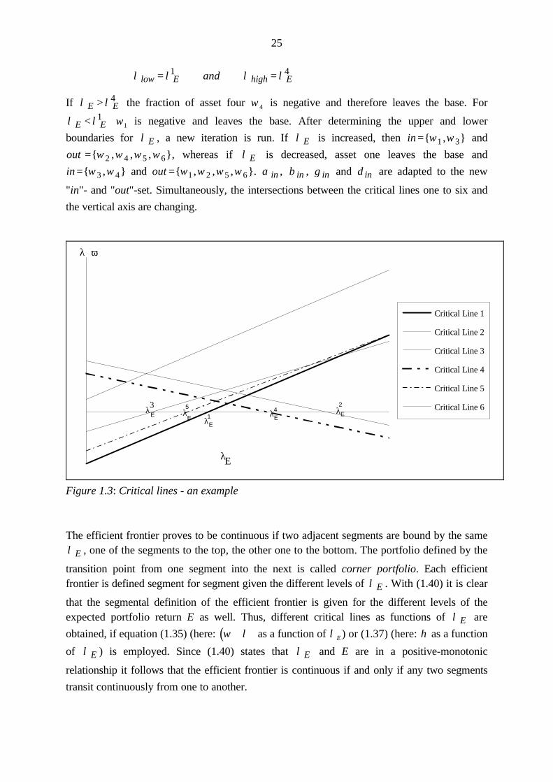
Under these assumptions, critical lines may be presented in the following figure. It elucidates
under which circumstances a variable leaves or enters the base.
From figure 1.3 it becomes clear that λ E is bounded to the bottom by λ E1 and to the top by
λ E4 , which implies:
25
λ λ λ λlow E high Eand= =1 4
If λ λE E> 4 the fraction of asset four ω 4 is negative and therefore leaves the base. For
λ λE E< 1 ω1 is negative and leaves the base. After determining the upper and lower
boundaries for λ E , a new iteration is run. If λ E is increased, then in ={ , }ω ω1 3 and
out ={ , , , }ω ω ω ω2 4 5 6 , whereas if λ E is decreased, asset one leaves the base and
in ={ , }ω ω3 4 and out ={ , , , }ω ω ω ω1 2 5 6 . α in , β in , γ in and δ in are adapted to the new
"in"- and "out"-set. Simultaneously, the intersections between the critical lines one to six and
the vertical axis are changing.
Critical Line 1
Critical Line 2
Critical Line 3
Critical Line 4
Critical Line 5
Critical Line 6
λ
3λλ λE5
14λ
2
EE
E E
λE
λ ω
Figure 1.3: Critical lines - an example
The efficient frontier proves to be continuous if two adjacent segments are bound by the sameλ E , one of the segments to the top, the other one to the bottom. The portfolio defined by the
transition point from one segment into the next is called corner portfolio. Each efficientfrontier is defined segment for segment given the different levels of λ E . With (1.40) it is clear
that the segmental definition of the efficient frontier is given for the different levels of theexpected portfolio return E as well. Thus, different critical lines as functions of λ E are
obtained, if equation (1.35) (here: ( )ω λ as a function of λE ) or (1.37) (here: η as a function
of λ E ) is employed. Since (1.40) states that λ E and E are in a positive-monotonic
relationship it follows that the efficient frontier is continuous if and only if any two segments
transit continuously from one to another.
26
Let a and b represent two critical lines which express two adjacent segments. Segment a is
defined for greater λ E than segment b. Defining λ highb as λ high of segment b according to
(1.39) and λ lowa as λ low of the adjacent segment a then a sufficient condition for continuity is:
(1.45) λ λlowa
highb=
In case (1.45) the critical lines representing segment a and b, respectively, would have anintersection. Because of (1.40) the continuity of λ E required by (1.45) implies the continuity
of E and (1.30 e) implies the continuity of ω along the efficient frontier. More specifically, the
equality of the composition of the portfolio in segment a for λ E = λ lowa and of the porfolio of
segment b for λ E = λ highb must be proven. Obviously this implies that the equality of the
expected returns and variances at the borders of segment a and b is given, respectively. Let
0(l) denote a zero-vector of dimension l the equation (1.30 a) may be expressed slightly
differently as:
(1.46)V A
A bin in in
inE
n′
=
µωλ
λ0 0
0( )
Without any loss of generality a specific asset k can be assumed to leave the base. This implies
ω k changes from "in" to "out", if E and equivalently λE moves from segment a into segment
b. It therefore holds:
( ) ( )∃ =≤ ≤1
0k n
k lowa
k highbandω λ η λ = 0
where ( )ω λk lowa denotes the portfolio fraction of asset k in segment a for λ λE low
a= and
( )η λk highb the partial derivative of the Lagrangian with respect to ωk given λ λE high
b= .
Furthermore, it can without loss of generality be assumed that the variables are sorted such,
that asset k is the element n of the vector of portfolio fractions ω . Furthermore, v' is defined as
a vector of dimension n which includes the covariances of returns of all assets with asset n,V n( )−1 the variance-covariance matrix of dimension n-1 including just the first n assets, A n( )−1
the first n-1 columns of A, α the last column, µ ( )n−1 , ω ( )n−1 the first n-1 lines of µ and ω ,
27
respectively. The variance of returns, expected return and fraction of asset n is denoted by σ n2 ,
µ n , and ω n . The former definitions may be analytically stated as:
(1.47) ( )v VV v
vn n n n in
n
n' ... ,
( )≡ ≡′
−
−σ σ σσ1 1
2 12
µµ
µ≡
−( )n
n
1 ωω
ω≡
−( )n
n
1 ( )A A n≡ −( )1 α
Substituting these definitions into (1.46) yields:
(1.48)
V v A
v
A b
n n n
n n
n
n
n
E
n( ) ( ) ( )
( )
( )( )− − −
−
−−′
′ ′
=
1 1 12
1
11
0 0
0
0
µ
σ α µα
ωωλ
λ
First of all, critical line b is examined. Here, ωn=ωk is non-base variable which implies:
(1.49) v n n= = = =0 1 0 02σ α µ
In addition to (1.49), employing (1.29 a) together with (1.37) allows the following statement:
( ) ( )η λ σ α µ
ω
ωλλ
n highb
n n
nb
nb
b
highb
v= ′ ′
−
=
−
2
1
0
( )
Using this equation for λ λEb
highb= and summarizing it with (1.48) and (1.49) it is obtained:
28
(1.50)
V A
A
v
b
n n n
n
n n
nb
nb
b
highb
n( ) ( )'
( )
( )
( ) ( )
' '
− − −
−
− −
−
=
1 1 1
12
1 10
0 1 0 0
0 0 0
0
0
0
µ
σ α µ
ω
ωλλ
In a further step, critical line a is considered. It is known that for λ λ λE Ea
lowa= = the asset k
which leaves the base ( )ω λk E equals zero. Thus, the former statement may be expressed by:
( )0 1 0 0 01 1
1
( )'
( )'
( )
n m
na
na
a
lowa
− −
−
−
=
ω
ωλλ
Comprising the realization from (1.48) for λ λEa
lowa= , a further transformation may be:
V v A
v
A b
n n n
n n
n
na
na
a
lowa
n( ) ( )'
( )
( )
( ) ( )
' '− − −
−
− −
−
=
1 1 12
1
1 1
0 0
0 1 0 0
0
0
0
µ
σ α µα
ω
ωλλ
Since ( )ω λn lowa = 0 , the second column may be replaced by arbitrary values without any
changes in the result vector at the left hand side.
(1.51)
V A
v
A b
n n n
n n
n
na
na
a
lowa
n( ) ( )'
( )
( )
( ) ( )
' '− − −
−
− −
−
=
1 1 12
1
1 10
0 0 0
0 1 0 0
0
0
0
µ
σ α µ
ω
ωλλ
Since in the corner portfolio λ λhighb
lowa= , reversing the second and the last line of the matrix
on the left hand side and of the vector on the right hand side of (1.51) provides a system of
29
equations which is equal to (1.50)10. Thus, converging λ E to the borders of the segments a
and b, respectively, yields identical vectors ω , λ and scalar λ E .
(1.52)
ω
ωλλ
ω
ωλλ
( ) ( )nb
nb
b
highb
na
na
a
lowa
− −
−
=
−
1 1
From (1.52) it is clear that the values for λE are identical at the borders. Since the portfolio
fractions are identical and since ( ) ( ) ( ) ( )ω λ ω λ ω λ ω λn lowa
k lowa
n highb
k highb= = = = 0 the
expected returns in both segments are equal. The efficient frontier is continuous.
2.5. Differentiating the efficient frontier
One of the properties of the ordinary efficient frontier given by (1.6) is that it is differentiable
in each point and strictly concave. This part shows that in the case restrictions a non-
differentiable efficient frontier is obtained. Although this was not proved by Markowitz [1987]
this seems to be an important insight. The third chapter will deal with shortfall risk
approaches. Since they are based on tangents to the efficient frontier, it is a matter of great
interest whether the efficient frontier is differentiable or not. It is vital to bear in mind that the
efficient frontier is composed of segments. Within each segment a specific portfolio is defined
by the "in"-set. Thus, within segments defined by intervals λ λ λE low high∈ , the efficient
frontier is defined by (1.6) and which implies that it is differentiable. Therefore, it is sufficient
to check differentiability at the corner portfolios.
Let ein represent the unity vector where elements are replaced by 0 if the respective variable is
contained in "out". Then, the derivative of the variance of the portfolio with respect to the
expected portfolio return for any λ λ λE low high∈ , may be expressed as11:
10 Markowitz [1987], p.171
11 see Merton [1972] and (1.6)
30
(1.53) ( )∂σ
∂ λ
2
E E
= 2 21 1
1 1 1 1( ) ( )
( )( ) ( ) ( )
' '
' ' ' 'e V e E V e
V e V e V e V ein in in in in in
in in in in in in in in in in in in
− −
− − − −−
−µ
µ µ µ µ
Obviously, the ratio changes depending on the segment which defines λE . Since µin, Vin and
ein are dependent on the elements of "in" and "out", for different λE (and consequently for
different E), different λE and different slopes can be expected.
To prove that the efficient frontier is not differentiable, it is sufficient to find a counter-
example. With respect to the former analysed circumstances this is not very difficult, if one
considers a portfolio consisting of three assets. Without loss of generality it may be assumed
that asset one first of all is included in "in" but moving to "out" as soon as the adjacentsegment is entered. Let vij represent element of line i and column j of the matrix Vin
−1 then the
expression e V ein in in' −1 of the above equation may be restated as:
e V ein in in' −1 = vij
j
n
i
n
==∑∑
11
If on the other hand asset one is excluded then
e V ein in in' −1 = v v v v22 23 32 33+ + +
Obviously, both expression are not equal, unless v v11 12 0+ = . This proves that
( )∂σ ∂ λ2 / E E in (1.53) differs for two adjacent segments which implies that the slopes of the
efficient frontier in two adjacent segments differ. In conclusion, the efficient frontier at the
corner portfolios is not differentiable.
2.6. Concavity and minimum variance portfolio
The unrestricted efficient frontier following (1.6) is characterized by strict concavity (Merton
[1972]). As was the case in the previous part strict concavity of the efficient frontier is a
property which will be needed for implementing shortfall risk based algorithms: if the efficient
frontier were not strictly concave but linear constructing tangents would be impossible. This
part confirms that concavity is also a characteristic of the restricted efficient frontier. Satisfying
31
the Kuhn-Tucker conditions (1.29) implies restricting λE by λ λ λE low high∈ , . Choosing an
expected portfolio return E, fixed and consistent with the interval for λE , a simpler formation
of optimization problem (1.25) can be stated:
(1.54) a) min 'ω
σ ω ω2 = V
b) µωω
''e
E=
This implies the following Lagrangian L'
(1.55) L E' = σ λ2 - E
with optimality condition:
(1.56)∂∂
∂ σ
∂λ λ
∂ σ
∂LE E EE E'= ⇔ − = ⇔ =0 0
2 2
Thus, the slope of the efficient frontier decreases with λE . Since (1.40) states that increasing
λE corresponds to increasing expected return E, the slope of the efficient frontier is negatively
related to expected returns. This is usually called strict concavity. This part showed that the
efficient frontier is strictly concave even if restrictions are imposed on the feasible set. The
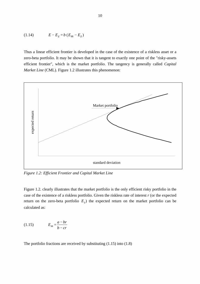
following figure illustrates that the restricted efficient frontier is composed by several efficient
frontiers, one defined for each segment. Furthermore, it shows intuitively that this fact implies
concavity.
32
standard deviation
expe
cted
ret
urn restricted efficient frontier
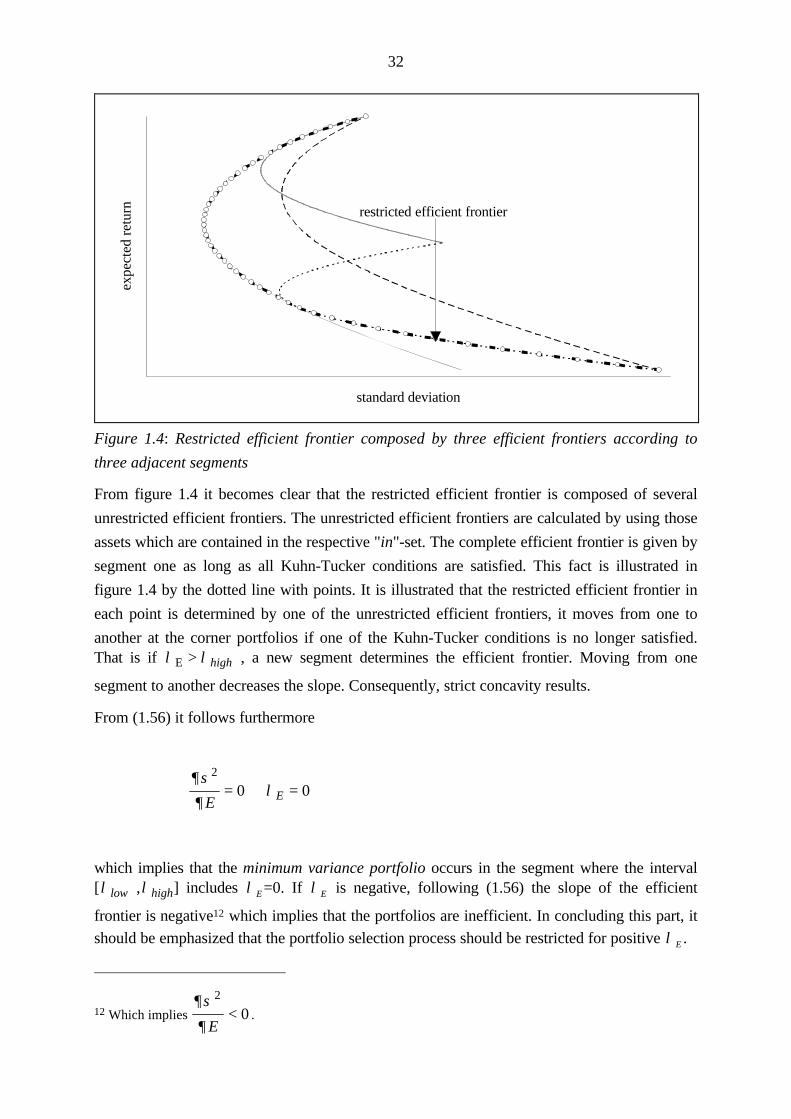
Figure 1.4: Restricted efficient frontier composed by three efficient frontiers according to
three adjacent segments
From figure 1.4 it becomes clear that the restricted efficient frontier is composed of several
unrestricted efficient frontiers. The unrestricted efficient frontiers are calculated by using those
assets which are contained in the respective "in"-set. The complete efficient frontier is given by
segment one as long as all Kuhn-Tucker conditions are satisfied. This fact is illustrated in
figure 1.4 by the dotted line with points. It is illustrated that the restricted efficient frontier in
each point is determined by one of the unrestricted efficient frontiers, it moves from one to
another at the corner portfolios if one of the Kuhn-Tucker conditions is no longer satisfied.That is if λ λE > high , a new segment determines the efficient frontier. Moving from one
segment to another decreases the slope. Consequently, strict concavity results.
From (1.56) it follows furthermore
∂ σ
∂λ
2
0 0E E= ⇔ =
which implies that the minimum variance portfolio occurs in the segment where the interval[λ low ,λhigh] includes λE =0. If λE is negative, following (1.56) the slope of the efficient
frontier is negative12 which implies that the portfolios are inefficient. In concluding this part, it
should be emphasized that the portfolio selection process should be restricted for positive λE .
12 Which implies ∂ σ
∂
2
0E
< .
33
2.7. Feasible base solution
Finding an initial feasible base solution is the condition for an application of the critical line
algorithm. First, an efficient combination of portfolio assets has to be found in order to fix the
initial sets "in" and "out". In the case of the ordinary Markowitz algorithm, which is the topic
of this section, a simple solution can be applied: By definition, each portfolio with maximum
available expected return is efficient. Thus, a feasible solution may be found by executing the
following program:
(1.57) max ' s. t. A = b 0ω
ω µ ω ω ≥
Then, the initial solution is { }in = 0 and solves (1.57)ω ω≥ . By applying (1.38) and
(1.39) λ low and λhigh are obtained; the algorithm can then be continued as stated in the present
section. In the special case of the ordinary Markowitz algorithm a trivial solution of (1.57) is
obtained, if the only asset which initially enters the base is that with the highest expected
return. This naturally maximizes the expected return on the portfolio. Since this is the case only
when non-negativity and equality restrictions are imposed for more general inequality
restrictions (1.57) has to be solved by the simplex approach. This will be comprehensively
discussed in the next section.
2.8. A numerical application
A portfolio optimization problem for three portfolio assets A, B and C which are defined as in
table 1.1. is considered.
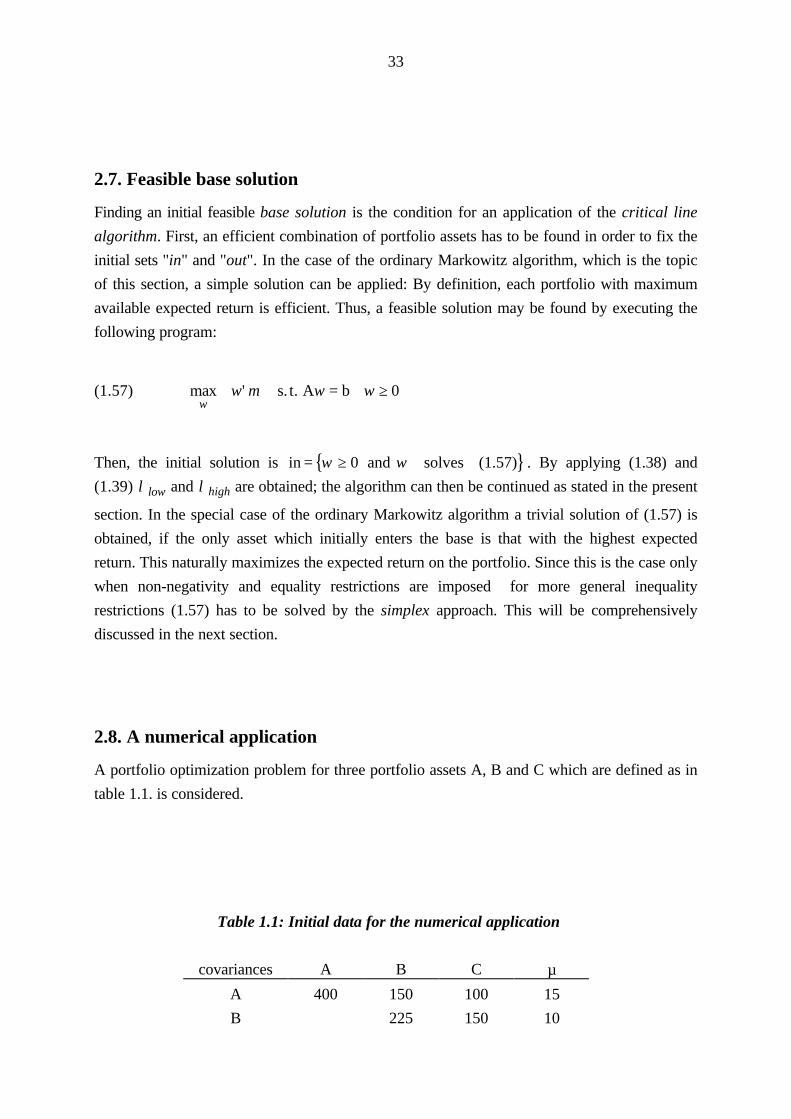
Table 1.1: Initial data for the numerical application
covariances A B C µA 400 150 100 15
B 225 150 10
34
C 625 20
The program which has to be executed is assumed to determine efficient portfolios subject to
the constraints that the portfolio fractions sum up to unity and that short sales are prohibited:
min 'ω
σ ω ω2 = V
( )1 1 1 11
2
3
ωωω
=
ω ≥0
According to the notation used thus far it may be defined:
V ≡
400 150 100
150 225 150
100 150 625
µ ≡
15
10
20
( )A ≡ 1 1 1
first step: determining a feasible base solution
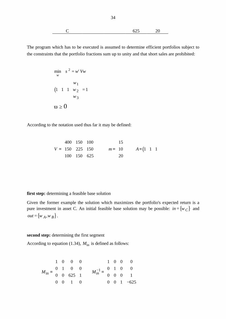
Given the former example the solution which maximizes the portfolio's expected return is apure investment in asset C. An initial feasible base solution may be possible: { }in C= ω and
{ }out A B= ω ω, .
second step: determining the first segment
According to equation (1.34), Min is defined as follows:
M Minin ≡
⇒ ≡
−
−
1 0 0 0
0 1 0 0
0 0 625 1
0 0 1 0
1 0 0 0
0 1 0 0
0 0 0 1
0 0 1 625
1
35
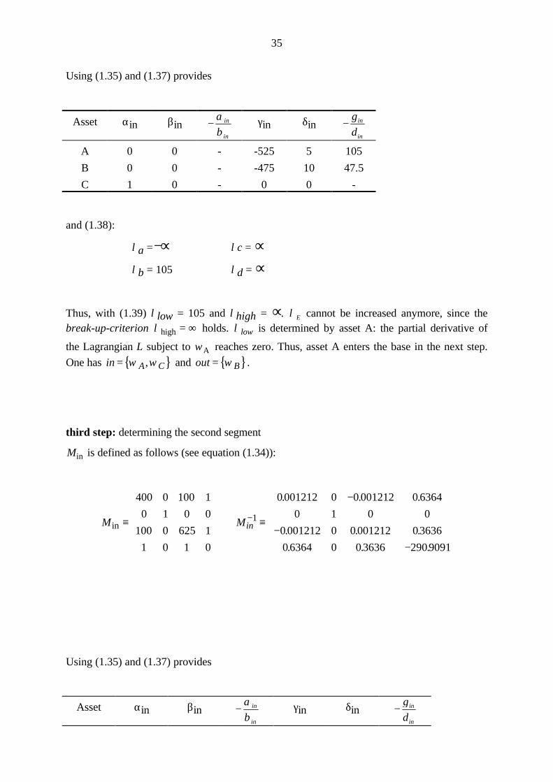
Using (1.35) and (1.37) provides
Asset αin βin −αβ
in
in
γin δin −γδ
in
in
A 0 0 - -525 5 105
B 0 0 - -475 10 47.5
C 1 0 - 0 0 -
and (1.38):
λa =−∞ λc = ∞λb = 105 λd = ∞
Thus, with (1.39) λlow = 105 and λhigh = ∞. λE cannot be increased anymore, since thebreak-up-criterion λhigh = ∞ holds. λ low is determined by asset A: the partial derivative of
the Lagrangian L subject to ωA reaches zero. Thus, asset A enters the base in the next step.
One has { }in A C= ω ω, and { }out B= ω .
third step: determining the second segment
Min is defined as follows (see equation (1.34)):
M Minin ≡
⇒ ≡
−
−−
−
400 0 100 1
0 1 0 0
100 0 625 1
1 0 1 0
0 001212 0 0 001212 0 6364
0 1 0 0
0 001212 0 0 001212 03636
0 6364 0 0 3636 2909091
1
. . .
. . .
. . .
Using (1.35) and (1.37) provides
Asset αin βin −αβ
in
in
γin δin −γδ
in
in
36
A 0.6364 -0.006061 105 0 0 -
B 0 0 - -140.9031 6.8182 20.67
C 0.3636 0.006061 -60 0 0 -
and (1.38):
λa = -60 λc = 105
λb = 20.67 λd = ∞
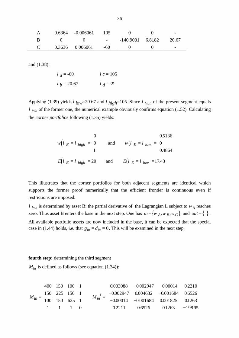
Applying (1.39) yields λlow=20.67 and λhigh=105. Since λhigh of the present segment equals
λ low of the former one, the numerical example obviously confirms equation (1.52). Calculating
the corner portfolios following (1.35) yields:
( ) ( )ω λ λ ω λ λE high E low= =
= =
0
0
1
0 5136
0
0 4864
and
.
.
( ) ( )E EE high E lowλ λ λ λ= = = =20 17 43and .
This illustrates that the corner portfolios for both adjacent segments are identical which
supports the former proof numerically that the efficient frontier is continuous even if
restrictions are imposed.
λ low is determined by asset B: the partial derivative of the Lagrangian L subject to ωB reaches
zero. Thus asset B enters the base in the next step. One has { }in A B C= ω ω ω, , and { }out = .
All available portfolio assets are now included in the base, it can be expected that the specialcase in (1.44) holds, i.e. that γ δin in= = 0 . This will be examined in the next step.
fourth step: determining the third segment
Min is defined as follows (see equation (1.34)):
M Minin ≡
⇒ ≡
− −− −− −
−
−
400 150 100 1
150 225 150 1
100 150 625 1
1 1 1 0
0 003088 0 002947 0 00014 0 2210
0 002947 0 004632 0 001684 0 6526
0 00014 0 001684 0 001825 01263
0 2211 0 6526 01263 19895
1
. . . .
. . . .
. . . .
. . . .
37
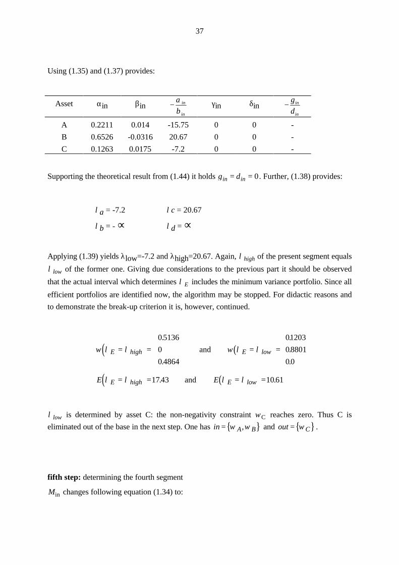
Using (1.35) and (1.37) provides:
Asset αin βin −αβ
in
in
γin δin −γδ
in
in
A 0.2211 0.014 -15.75 0 0 -
B 0.6526 -0.0316 20.67 0 0 -
C 0.1263 0.0175 -7.2 0 0 -
Supporting the theoretical result from (1.44) it holds γ δin in= = 0 . Further, (1.38) provides:
λa = -7.2 λc = 20.67
λb = - ∞ λd = ∞
Applying (1.39) yields λlow=-7.2 and λhigh=20.67. Again, λhigh of the present segment equals
λ low of the former one. Giving due considerations to the previous part it should be observed
that the actual interval which determines λ E includes the minimum variance portfolio. Since all
efficient portfolios are identified now, the algorithm may be stopped. For didactic reasons and
to demonstrate the break-up criterion it is, however, continued.
( ) ( )ω λ λ ω λ λE high E low= =
= =
0 5136
0
0 4864
01203
08801
0 0
.
.
.
.
.
and
( ) ( )E EE high E lowλ λ λ λ= = = =17 43 10 61. .and
λ low is determined by asset C: the non-negativity constraint ωC reaches zero. Thus C is
eliminated out of the base in the next step. One has { }in A B= ω ω, and { }out C= ω .
fifth step: determining the fourth segment
Min changes following equation (1.34) to:
38
M Minin ≡
⇒ ≡
−−
−
−
400 150 0 1
150 225 0 1
0 0 1 0
1 1 0 0
0 0031 0 0031 0 0 2308
0 0031 0 0031 0 0 7692
0 0 1 0
0 2308 0 7692 0 207 69
1
. . .
. . .
. . .
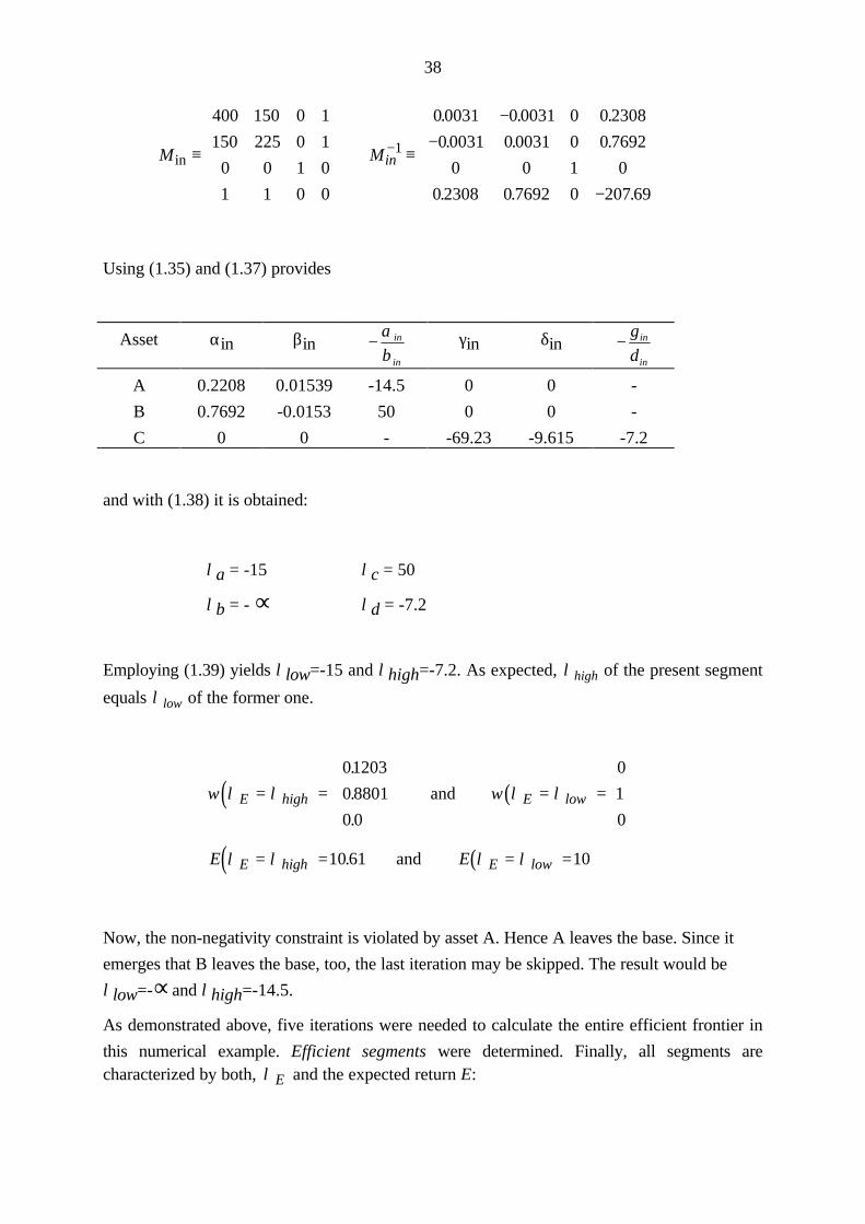
Using (1.35) and (1.37) provides
Asset αin βin −αβ
in
in
γin δin −γδ
in
in
A 0.2208 0.01539 -14.5 0 0 -
B 0.7692 -0.0153 50 0 0 -
C 0 0 - -69.23 -9.615 -7.2
and with (1.38) it is obtained:
λa = -15 λc = 50
λb = - ∞ λd = -7.2
Employing (1.39) yields λlow=-15 and λhigh=-7.2. As expected, λhigh of the present segment
equals λ low of the former one.
( ) ( )ω λ λ ω λ λE high E low= =
= =
01203
0 8801
0 0
0
1
0
.
.
.
and
( ) ( )E EE high E lowλ λ λ λ= = = =10 61 10. and
Now, the non-negativity constraint is violated by asset A. Hence A leaves the base. Since it
emerges that B leaves the base, too, the last iteration may be skipped. The result would be
λlow=-∞ and λhigh=-14.5.
As demonstrated above, five iterations were needed to calculate the entire efficient frontier in
this numerical example. Efficient segments were determined. Finally, all segments arecharacterized by both, λ E and the expected return E:
39
number of segment λhigh λlow E (λhigh) E (λlow)
1 ∞ 105 20.0 20.0
2 105 20.67 20.0 17.43
3 20.67 -7.2 17.43 10.61
4 -7.2 -14.5 10.61 10.0
5 -14.5 -∞ 10.0 10.0
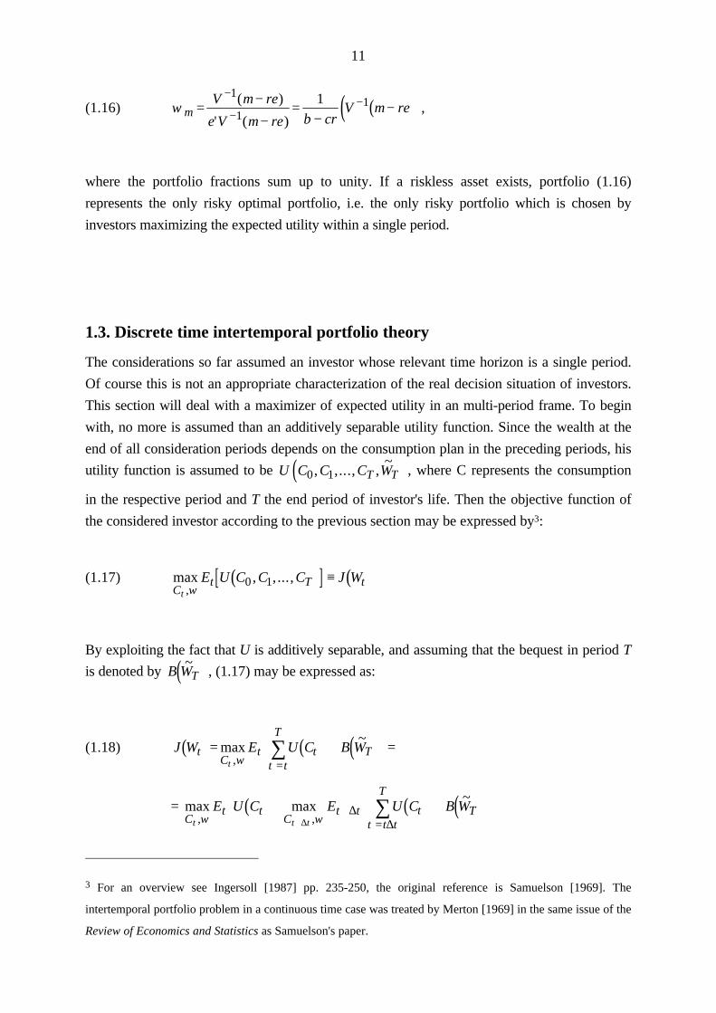
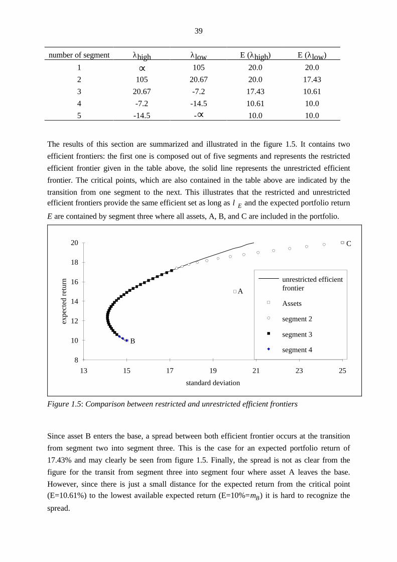
The results of this section are summarized and illustrated in the figure 1.5. It contains two
efficient frontiers: the first one is composed out of five segments and represents the restricted
efficient frontier given in the table above, the solid line represents the unrestricted efficient
frontier. The critical points, which are also contained in the table above are indicated by the
transition from one segment to the next. This illustrates that the restricted and unrestrictedefficient frontiers provide the same efficient set as long as λ E and the expected portfolio return
E are contained by segment three where all assets, A, B, and C are included in the portfolio.
standard deviation
expe
cted
ret
urn
8
10
12
14
16
18
20
13 15 17 19 21 23 25
unrestricted efficientfrontier
Assets
segment 2
segment 3
segment 4
A
B
C
Figure 1.5: Comparison between restricted and unrestricted efficient frontiers
Since asset B enters the base, a spread between both efficient frontier occurs at the transition
from segment two into segment three. This is the case for an expected portfolio return of
17.43% and may clearly be seen from figure 1.5. Finally, the spread is not as clear from the
figure for the transit from segment three into segment four where asset A leaves the base.
However, since there is just a small distance for the expected return from the critical point
(E=10.61%) to the lowest available expected return (E=10%=µB) it is hard to recognize the
spread.

40