algorithms for parallel memory, ii: hierarchical multilevel

Algorithmica (1994)12:148 169 Algorithmica �9 1994 Springer-Verlag New York Inc.

Algorithms for Parallel Memory, II: Hierarchical Multilevel Memories 1

J. S. Vitter 2 and E. A. M. Shriver 3

Abstract, In this paper we introduce parallel versions of two hierarchical memory models and give optimal algorithms in these models for sorting, FFT, and matrix multiplication. In our parallel models, there are P memory hierarchies operating simultaneously; communication among the hierarchies takes place at a base memory level. Our optimal sorting algorithm is randomized and is based upon the probabilistic partitioning technique developed in the companion paper for optimal disk sorting in a two-level memory with parallel block transfer. The probability of using l times the optimal running time is exponentially small in/(log/) log P.

Key Words. Memory hierarchies, Multilevel memory, Sorting, Distribution sort, FFT, Matrix multiplication, Matrix transposition.

1. Introduction. Large-scale computer systems contain many levels of memory-- ranging from very small but very fast registers, to successively larger but slower memories, such as multiple levels of cache, primary memory, magnetic disks, and archival storage. An elegant hierarchical memory model was introduced by Aggar- wal et al. [1] and further developed by Aggarwal et aI. [-23 to take into account block transfer. All computation takes place in the central processing unit (CPU), one instruction per unit time. Access to memory takes a varying amount of time, depending on how low in the memory hierarchy the memory access is. Optimal bounds are obtained in [-1] and 1-23 for several sorting and matrix-related problems.

In this paper we investigate the capabilities of parallel memory hierarchies. In the next section we define two uniform memory models, each consisting of P hierarchical memories connected together at their base levels. The P hierarchical memories can be either of the two types [13, 1-2] mentioned earlier.

For each model, we develop matching upper and lower bounds for the problems

A summarized version of this research was presented at the 22nd Annual ACM Symposium on Theory of Computing, Baltimore, MD, May 1990. This work was done while the first author was at Brown University. Support was provided in part by a National Science Foundation Presidential Young Investigator Award with matching funds from IBM, by NSF Research Grants DCR-8403613 and CCR-9007851, by Army Research Office Grant DAAL03-91-G-0035, and by the Office of Naval Research and the Defense Advanced Research Projects Agency under Contract N00014-91-J-4052 ARPA Order 8225. This work was done in part while the second author was at Brown University supported by a Bellcore graduate fellowship and at Bellcore. 2 Department of Computer Science, Duke University, Box 90129, Durham, NC 27708-0129, USA. 3 Courant Institute, New York University, 251 Mercer Street, New York, NY 10012, USA.

Received September 26, 1990; revised January 14, 1993. Communicated by C. K. Wong.


of sorting, FFT, and matrix multiplication, which are defined in Section 3. The algorithms that realize the optimal bounds for sorting are applications of the optimal disk sorting algorithm developed in the companion paper [11] for a two-level memory model with parallel block transfer. We apply the partitioning technique of [11] to the one-hierarchy sorting algorithms of [1] and [2]. Intui- tively, the hierarchical algorithms are optimal because the internal processing in the corresponding two-level algorithms is efficient. The main results are given in Section 4 and are proved in Sections 5-10. Conclusions and open problems are discussed in Section 11.

2. Parallel Hierarchical Memory Models. A hierarchical memory model is a uniform model consisting of memory whose locations take different amounts of time to access. The basic unit of transfer in the hierarchical memory model H M M [1] is the record; access to location x takes time f(x). The block transfer model BT [2] represents a notion of block transfer applied to H M M ; in the BT model, access to the t + 1 records at locations x - t, x - t + 1 . . . . . x takes time f ( x ) + t. Typical access cost functions are f (x ) = log x and f ( x ) = x ~, for some ~ > 0. A model similar to the BT model that allows pipelined access to memory in O(log n) time was developed independently by Luccio and Pagli [5].

We can think of a memory hierarchy as being organized into discrete levels, as shown in Figure 1 for H M M ; for each k > 1, level k contains the 2 k-1 locations at addresses 2 k- 1 2 k- 1 + 1 . . . . . 2 k - 1. We restrict our attention to well-behaved access costs f (x) , in which f ( x ) is nondecreasing and there are constants c and Xo such that f(2x) < cf(x), for all x > Xo. For such f (x) , access to any location on level k takes | time. The access cost functions f (x ) = log x and f ( x ) = x ~, for some ~ > 0, are well behaved. ~ For example, if f ( x ) = log x, access to any location on level k takes time ~ k.

Both the H M M and BT hierarchical memory models can be augmented to allow parallel data transfer. One possibility is to have a discretized hierarchy, in which each memory component is connected to P larger but slower memory

level 6 I I I

level 5 ] I

level 4 level 3

level 2 t level 1

IcPul Fig. 1. The HMM hierarchical memory model [1].

4 For simplicity of notation, we use log x, where x > 1, to denote the quantity max{l, log 2 x}.

150 J.S. Vitter and E. A. M. Shriver

r i

Fig. 2. A parallel hierarchical memory. The P individual memory hierarchies can be either of type HMM or of type BT, The P CPUs can communicate among one another via the network; we assume, for example, that the P records stored in their accumulators can be sorted in O(log P) time.

components at the next level. A cleaner and more feasible extension, which we adopt in this paper, is to have P separate memories connected together at the base level of each hierarchy. Our model is pictured in Figure 2.

More specifically, we assume that the P hierarchies can each function independently. Communication between hierarchies takes place at the base memory level (level 1), which consists of location 1 from each of the P hierarchies. We assume that the P base memory level locations are interconnected via a network such as a hypercube or cube-connected cycles so that the P records in the base memory level can be sorted in O(log P) time (perhaps via a randomized algorithm

[9]) and so that two x / ~ x x//ff/2 matrices stored in the base memory level

can be multiplied in O(x/~ ) time. We denote by P -H MM and P-BT the P- hierarchy variants of the hierarchical memory models H M M and BT, as described above.

We refer to the P locations, one per hierarchy, at the same relative position in each of the P hierarchies as a track, by analogy with the two-level disk model [11]. The ith track, for i > 1, consists of location i from each of the P hierarchies. In this terminology the base memory level is the track at location 1. The global memory locations (which refer collectively to the P hierarchies combined) are numbered track by track. That is, the global memory locations in track 1 are numbered 1, 2 . . . . . P; the global memory locations in track 2 are numbered P + 1, P § 2 , . . . , 2 P ; and so on.

3. Problem Definitions. The following definitions of sorting, FFT, and standard matrix multiplication are essentially those of the companion paper [11].

SORTING.

Problem Instance: The N records are stored in the first N global memory locations. Goal: The N records are stored in sorted nondecreasing order in the first N global

memory locations.


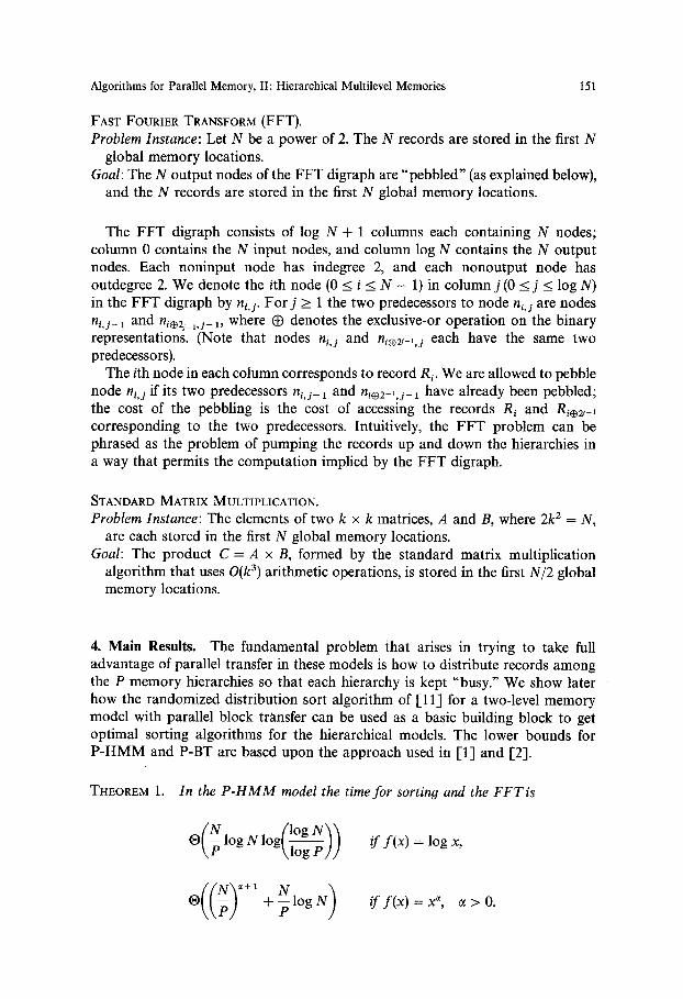
FAST FOURIER TRANSFORM (FFT). Problem Instance: Let N be a power of 2. The N records are stored in the first N

global memory locations. Goal: The N output nodes of the FFT digraph are "pebbled" (as explained below),

and the N records are stored in the first N global memory locations.

The FFT digraph consists of log N + 1 columns each containing N nodes; column 0 contains the N input nodes, and column log N contains the N output nodes. Each noninput node has indegree 2, and each nonoutput node has outdegree 2. We denote the ith node (0 < i < N - 1) in column j (0 < j < log N) in the FFT digraph by ni, j. For j > 1 the two predecessors to node n,,~ are nodes ni,j_, and ni@2j_,,j_l, where @ denotes the exclusive-or operation on the binary representations. (Note that nodes n~,j and n~ez_,,j each have the same two predecessors).

The ith node in each column corresponds to record R~. We are allowed to pebble node ni, ~ if its two predecessors ni, ~_ 1 and ni@z-l,j_ 1 have already been pebbled; the cost of the pebbling is the cost of accessing the records R~ and R~ez_, corresponding to the two predecessors. Intuitively, the FFT problem can be phrased as the problem of pumping the records up and down the hierarchies in a way that permits the computation implied by the FFT digraph.

STANDARD MATRIX MULTIPLICATION. Problem Instance: The elements of two k x k matrices, A and B, where 2k 2 = N,

are each stored in the first N global memory locations. Goal: The product C = A x B, formed by the standard matrix multiplication

algorithm that uses O(k 3) arithmetic operations, is stored in the first N/2 global memory locations.

4. Main Results. The fundamental problem that arises in trying to take full advantage of parallel transfer in these models is how to distribute records among the P memory hierarchies so that each hierarchy is kept "busy." We show later how the randomized distribution sort algorithm of [11] for a two-level memory model with parallel block transfer can be used as a basic building block to get optimal sorting algorithms for the hierarchical models. The lower bounds for P-HMM and P-BT are based upon the approach used in [1] and [2].

THEOREM 1. In the P - H M M model the time for sorting and the FFT i s

~(~- log N l o g ( ~ \Iog r l i if f (x) = log x,

/ I ' N ' X = + i + N l o g N ) ~ if f ( x ) = x ~, ot>O.


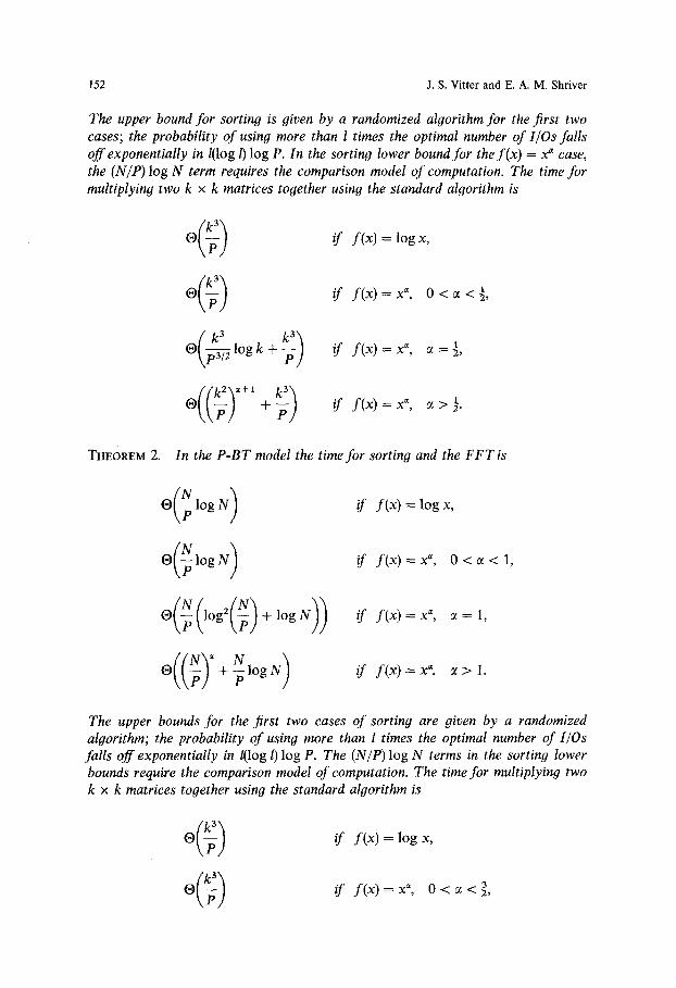
The upper bound for sorting is given by a randomized algorithm for the first two cases; the probability of using more than l times the optimal number of l/Os falls off exponentially in/(log/) log P. In the sorting lower bound for the f (x) = x ~ case, the (N/P)log N term requires the comparison model of computation. The time for multiplying two k x k matrices together using the standard algorithm is

0 l o g k + if f ( x ) = x ~, ct=�89

if f ( x ) = x ~, ~>�89

THEOREM 2. In the P-BT model the time for sorting and the FFTis

if f ( x ) = x ~, ~ = 1 ,

if f (x) ---= x ~, o: > 1.

The upper bounds for the first two cases of sorting are given by a randomized algorithm; the probability of using more than I times the optimal number of I/Os falls off exponentially in/(log/) log P. The (N/P) log N terms in the sorting lower bounds require the comparison model of computation. The time for multiplying two k x k matrices together using the standard algorithm is


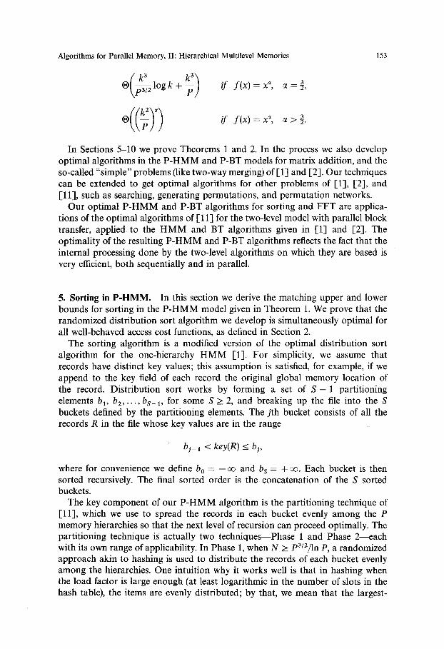
O(p~/2 log k + ~ - ) if f ( x ) = x ~, o~=~,

if f ( x ) = x ~, ~ > ~ .

In Sections 5-10 we prove Theorems 1 and 2. In the process we also develop optimal algorithms in the P-HMM and P-BT models for matrix addition, and the so-called "simple" problems (like two-way merging) of [1-1 and [2]. Our techniques can be extended to get optimal algorithms for other problems of [1], [2], and [11], such as searching, generating permutations, and permutation networks.

Our optimal P-HMM and P-BT algorithms for sorting and FFT are applications of the optimal algorithms of [11-1 for the two-level model with parallel block transfer, applied to the H M M and BT algorithms given in [1] and [2]. The optimality of the resulting P-HMM and P-BT algorithms reflects the fact that the internal processing done by the two-level algorithms on which they are based is very efficient, both sequentially and in parallel.

5. Sorting in P-HMM. In this section we derive the matching upper and lower bounds for sorting in the P-HMM model given in Theorem 1. We prove that the randomized distribution sort algorithm we develop is simultaneously optimal for all well-behaved access cost functions, as defined in Section 2.

The sorting algorithm is a modified version of the optimal distribution sort algorithm for the one-hierarchy H M M [1]. For simplicity, we assume that records have distinct key values; this assumption is satisfied, for example, if we append to the key field of each record the original global memory location of the record. Distribution sort works by forming a set of S - 1 partitioning elements b 1, b E . . . . . b s _ l , for some S > 2, and breaking up the file into the S buckets defined by the partitioning elements. The j th bucket consists of all the records R in the file whose key values are in the range

b j_ x < key(R) <_ b j,

where for convenience we define b o = - o e and b s = + oo. Each bucket is then sorted recursively. The final sorted order is the concatenation of the S sorted buckets.

The key component of our P-HMM algorithm is the partitioning technique of [11], which we use to spread the records in each bucket evenly among the P memory hierarchies so that the next level of recursion can proceed optimally. The partitioning technique is actually two techniques--Phase 1 and Phase 2----each with its own range of applicability. In Phase 1, when N > P3/Z/ln P, a randomized approach akin to hashing is used to distribute the records of each bucket evenly among the hierarchies. One intuition why it works well is that in hashing when the load factor is large enough (at least logarithmic in the number of slots in the hash table), the items are evenly distributed; by that, we mean that the largest-


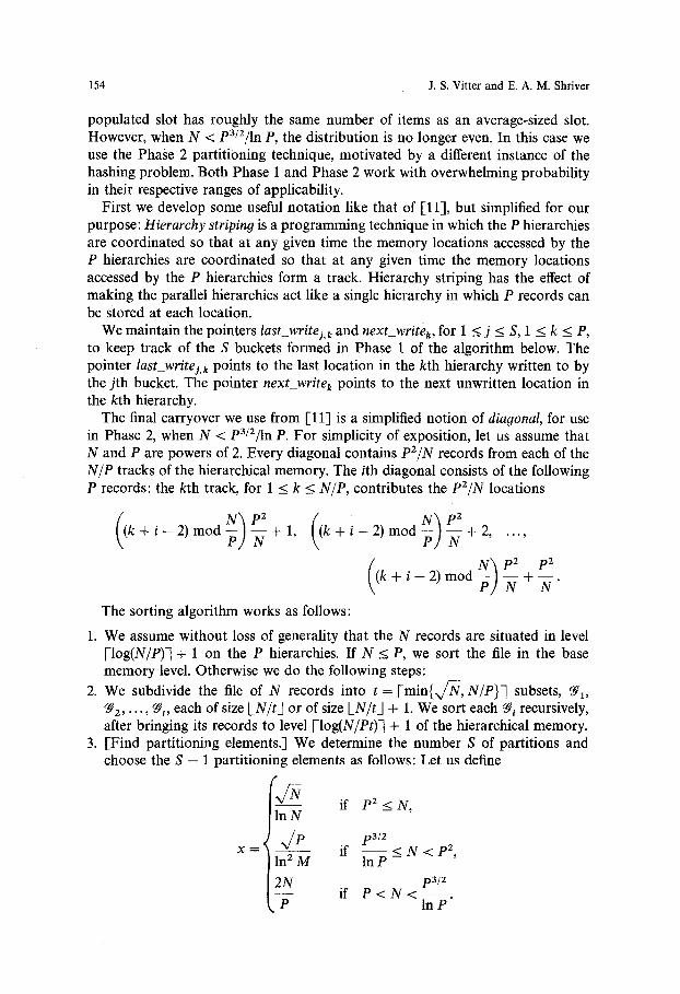
populated slot has roughly the same number of items as an average-sized slot. However, when N < P3/E/ln P, the distribution is no longer even. In this case we use the Phase 2 partitioning technique, motivated by a different instance of the hashing problem. Both Phase 1 and Phase 2 work with overwhelming probability in their respective ranges of applicability.

First we develop some useful notation like that of [11], but simplified for our purpose: Hierarchy striping is a programming technique in which the P hierarchies are coordinated so that at any given time the memory locations accessed by the P hierarchies are coordinated so that at any given time the memory locations accessed by the P hierarchies form a track. Hierarchy striping has the effect of making the parallel hierarchies act like a single hierarchy in which P records can be stored at each location.

We maintain the pointers last_writej.k and next_writek, for 1 _ j _ S, 1 _< k _ P, to keep track of the S buckets formed in Phase I of the algorithm below. The pointer last_writej, k points to the last location in the kth hierarchy written to by the j th bucket. The pointer next writek points to the next unwritten location in the kth hierarchy.

The final carryover we use from [11] is a simplified notion of diagonal, for use in Phase 2, when N < p3/2/ln P. For simplicity of exposition, let us assume that N and P are powers of 2. Every diagonal contains p2/N records from each of the NIP tracks of the hierarchical memory. The ith diagonal consists of the following P records: the kth track, for 1 < k < N/P, contributes the p2/N locations

(k + i - 2) mod ~ - + 1, (k + i - 2) mod ~ - + 2 . . . . .

(k + i - 2) mod ~ - + ~ - .

The sorting algorithm works as follows:

1. We assume without loss of generality that the N records are situated in level Flog(N/P)-] + 1 on the P hierarchies. If N _< P, we sort the file in the base memory level. Otherwise we do the following steps:

2. We subdivide the file of N records into t = [-min{x/~, N/P}-] subsets, ~r N2, . - . , Nt, each of size IN~t_] or of size LN/tJ + 1. We sort each Ni recursively, after bringing its records to level [-log(N/Pt)-] + 1 of the hierarchical memory.

3. [Find partitioning elements.] We determine the number S of partitions and choose the S - 1 partitioning elements as follows: Let us define

In N

x = x/P In 2 M

2N

P

if P2 <_ N,

p3/2 if - - ~ N < p2,

In P p3/2

if P < N < In P"


We form a set A of at least N/log N elements consisting of the key value of every tlog NJth record from each f#/. We sort A using two-way merge sort with hierarchy striping. We set S to be LIAWLIAI/x]] + 1 ,~ x. We define the j th partitioning element bj, for each 1 < j < S - 1, to be the jklAI/xJth smallest element of A. We move the partitioning elements to level [log(S/P)7 + 1.

4. [Phase 1 or Phase 2?] If N > Pa/2/lnP, we do Step 5 corresponding to Phase 1; otherwise we do Steps 6 and 7, corresponding to Phase 2.

5. [Phase 1.] For each 1 < i < t in sequence, we partition fgi by processing it in sorted order. We move P records at a time to the base memory level and determine which bucket each record belongs to by merging in the partitioning elements. The partitioning elements can be processed P elements at a time, so that the merging proceeds optimally; when the next track of partitioning elements is needed, it is read into the base memory level. We then randomly scramble the P records and write the records back to level [-log(N/P)7 + 1. If the record written in the kth hierarchy belongs to the jth bucket ~ , we update the pointers last_writej, k and next_writek, which are stored in hierarchy k, so that all the records of each bucket are linked together in the hierarchy, which is necessary for the next recursive application of the algorithm. We then proceed to Step 8.

6. [-Phase 2--Pass 1.] We scramble the N records, P at a time, by reading the file to the base memory level, track by track, randomly permuting the P records there, and writing them back to level [log(N/P)7 + 1.

7. [Phase 2--Pass 2.] We move P records at a time to the base memory level, one diagonal at a time, as defined above. For each diagonal of P records, we partition the records into buckets by sorting the P records and the partitioning elements. (The number of partitioning elements is 2N/P < P, for P > 4.) We write the P records back to level Flog(N/P)q + 1, cycling through the buckets; if a bucket is empty, a dummy record is written. Let d be the least common multiple of P and S. After every d/S cycles of P writes, we skip over the next hierarchy before beginning the next cycle of P writes.

8. [Sort recursively.] For each 1 < j < S in sequence, we sort the j th bucket recursively, after bringing the records of ~ to level Flog(N/SP)q + 1 of the hierarchical memory. (With high probability, the records in each bucket are distributed evenly among the P hierarchies, and thus each bucket can be accessed in O((N/SP)f(N/P)) time.) The sorted list of N records consists of the concatenated sorted buckets.

The value of x in Step 3, which determines the number of partitioning elements, is chosen so that the partitioning analysis from the companion paper [11] can be modified to show that the records with high probability are distributed evenly among the buckets.

5.1. Logarithmic Access Cost. Let us first consider the case f ( x ) = log x of Theorem 1.

THEOREM 3. The time used by the above algorithm to sort N >_ P records in the

156 J.S. vitter and E. A. M. Shriver

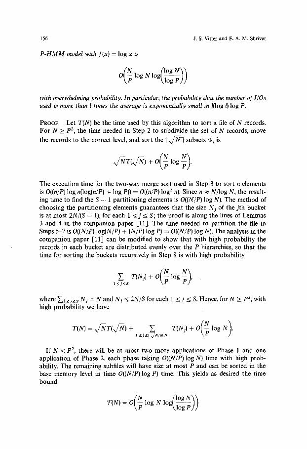
P-HMM model with f(x) = log x is

�9 / l o g O( N log N , o g ~ J J

with overwhelming probability. In particular, the probability that the number of I/Os used is more than l times the average is exponentially small in/(log/) log P.

PROOF. Let T(N) be the time used by this algorithm to sort a file of N records. For N > p2, the time needed in Step 2 to subdivide the set of N records, move

the records to the correct level, and sort the [-x/-N-] subsets f#, is

x/~T(w/N) + o ( N log N).

The execution time for the two-way merge sort used in Step 3 to sort n elements is O((n/P) log n(log(n/P) + log P)) = O((n/P) log 2 n). Since n ~ N/log N, the resulting time to find the S - 1 partitioning elements is O((N/P) log N). The method of choosing the partitioning elements guarantees that the size Nj of the jth bucket is at most 2N/(S - 1), for each 1 < j < S; the proof is along the lines of Lemmas 3 and 4 in the companion paper [11]. The time needed to partition the file in Steps 5-7 is O((N/P) log(N/P) + (N/P) log P) = O((N/P) log N). The analysis in the companion paper [11] can be modified to show that with high probability the records in each bucket are distributed evenly over the P hierarchies, so that the time for sorting the buckets recursively in Step 8 is with high probability

l_<j_<s ~ log ,

where ~1 <_s<_s Nj = N and Ni <_ 2N/S for each 1 < j < S. Hence, for N > p 2 with high probability we have

T(N) = x/~T(xfN) + ~ T(Nj) + O( N ) 1 <_jz~/N/lnN~ ~ log N .

If N < p2, there will be at most two more applications of Phase 1 and one application of Phase 2, each phase taking O((N/P)log N) time with high probability. The remaining subfiles will have size at most P and can be sorted in the base memory level in time O((N/P)log P) time. This yields as desired the time bound

N , f l o g T(N) = 0 ~ log N l o g ~ j j


with high probability. The probability bounds quoted in Theorem 3 follow from those in [11]. []

The following lower bound matches the algorithm's running time in Theorem 3, and thus the algorithm is optimal. It is interesting to note that this lower bound, as well as several others in this paper, ignores the cost of the network communication and considers only the cost of memory access.

THEOREM 4 . The time required to sort N > P records in the P - H M M model with f (x ) = log x is

, flog N~'~ f~(N log N l o g t ~ ) ) .

PROOF. Let A be a sorting algorithm that is optimal in the P-HMM model. Let us define the "sequential time" of A to be the sum of its time costs for each of the P hierarchies; the sequential time of A is at most P times its running time. Following the approach in [1], we can imagine superimposing onto the P-HMM- type hierarchical memory a sequence of two-level memories. For each M in the range P < M < N, we superimpose on the P-HMM an internal memory of size M and one infinite-sized disk.

By [3], the I/O complexity of sorting N records with one disk, no blocking, and an internal memory of size M is

(1) Tu(N) = nfN\ logl~ M).

The " - M " term permits M records to reside initially in the internal memory. In each individual hierarchy every transfer done by A that corresponds to an I/O with respect to an internal memory of size M contributes

' :(7) :(7) to its sequential time. In other words, if we let T:(N) denote the sequential time for A, we have

,2,

158 J.s. vitter and E. A. M. Shriver

Forf (x) = log x, we have 6f(M/P) = log((M + 1)/M) --- | Plugging this and (1) into (2) we get

= f~ ~ 1) ) log N TI(N) (V<~t<N ( N I ~ = ~ ( N , / l ogN '~ ,

Dividing the sequential time TI(N ) by P gives us the desired lower bound. []

5.2. Other Access Costs. First we show the lower bound corresponding to case f (x ) = x ~, for ~ > 0, of Theorem 1:

THEOREM 5. The time required to sort N >_ P records in the P - H M M model with f (x ) = x ~, for ct > O, is

N N)

The (N/P) log N term depends on using the comparison model of computation.

PROOF. We apply the same approach as in Theorem 4, except that we use f (x ) = x ~. Substituting 6f (m/P) = | ~- lIP 0 and (1) into (2), we get

Dividing the sequential time Ts(N ) by P gives us the first term of the desired lower bound. The second term follows from the N log N lower bound for sorting in the comparison model of computation. []

The next theorem shows that the sorting algorithm given earlier in Section 5 is uniformly optimal (in the language of [1]) in that it is optimal for all well-behaved access costs f(x) , as defined in Section 2. In particular, it follows that the sorting algorithm's running time for the case f ( x ) = x ~, where e > 0, meets the lower bound of Theorem 5 and is therefore optimal. The following theorem, when combined with Theorem 4, also gives an alternate proof of Theorem 3.

THEOREM 6. The algorithm given at the beginning of Section 5 is optimal for all well-behaved access costs f(x).

PROOF. We use a parallelized version of the approach of rl], combined with the lower bound strategy of Theorems 4 and 5. Let T~t.v(N) be the average number of I/O steps done by the sorting algorithm with respect to an internal memory of


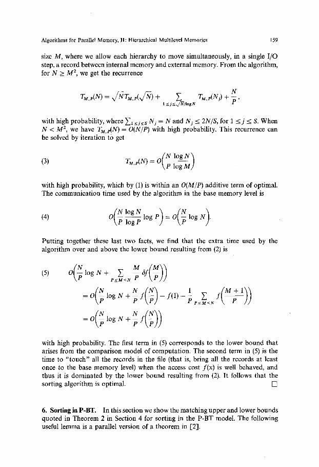
size M, where we allow each hierarchy to move simultaneously, in a single I/O step, a record between internal memory and external memory. From the algorithm, for N > M 2, we get the recurrence

rM , (N) = + N

2 TM, p(Nj) + 1 <_j<_x~/logN

with high probability, where ~1 _<j_<s Nj = N and Nj <_ 2N/S, for 1 _ j _< S. When N < M 2, we have TM, e(N) = O(N/P) with high probability. This recurrence can be solved by iteration to get

(3)

with high probability, which by (1) is within an O(M/P) additive term of optimal. The communication time used by the algorithm in the base memory level is

( l~ ) (4) 0 log P ~ log N .

Putting together these last two facts, we find that the extra time used by the algorithm over and above the lower bound resulting from (2) is

( 5 ) O F l ~ Z ~ - 6 f P<M<N

1 = O ~ l o g N + ~ f -- f (1)-- ~

P<M<N

= 0 F l o g N + F f

with high probability. The first term in (5) corresponds to the lower bound that arises from the comparison model of computation. The second term in (5) is the time to "touch" all the records in the file (that is, bring all the records at least once to the base memory level) when the access cost f(x) is well behaved, and thus it is dominated by the lower bound resulting from (2). It follows that the sorting algorithm is optimal. []

6. Sorting in P-BT. In this section we show the matching upper and lower bounds quoted in Theorem 2 in Section 4 for sorting in the P-BT model. The following useful lemma is a parallel version of a theorem in [2].


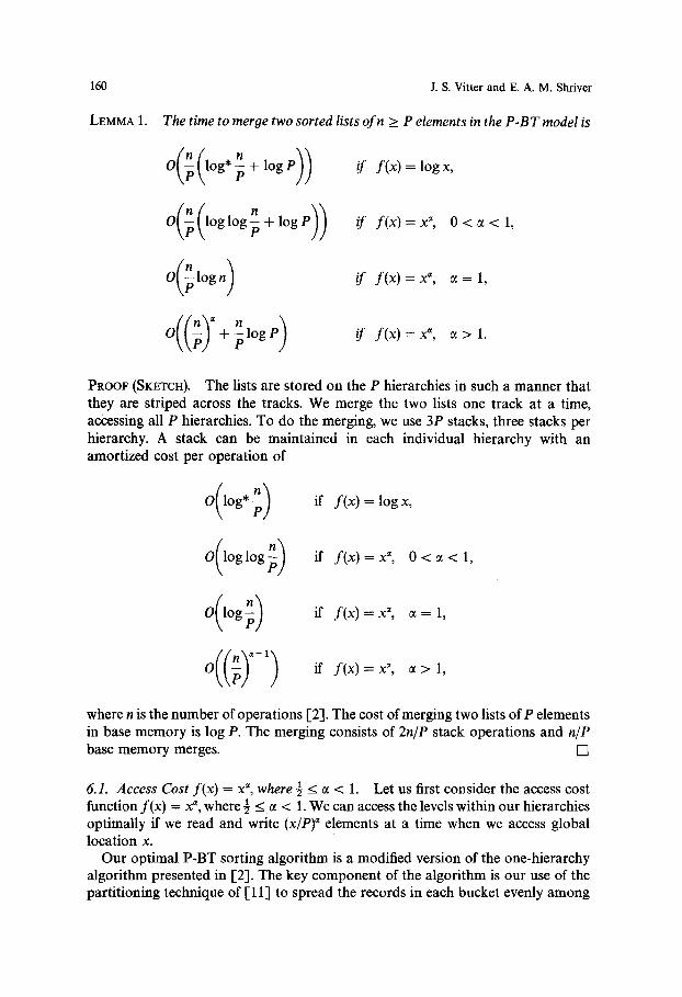
LEMMA 1. The time to merge two sorted lists of n >_ P elements in the P - B T model is

//n// , n if f ( x ) = log x,

if f ( x ) = x ~, 0 < ~ < 1 ,

O + ~ l o g P if f ( x ) = x ' , ~ > 1.

PROOF (SKETCH). The lists are stored on the P hierarchies in such a manner that they are striped across the tracks. We merge the two lists one track at a time, accessing all P hierarchies. To do the merging, we use 3P stacks, three stacks per hierarchy. A stack can be maintained in each individual hierarchy with an amortized cost per operation of

if

O ( l o g p ) if f ( x ) = x~, ~ = 1 ,

O if f ( x ) = x ~, ~ > 1 ,

where n is the number of operations [2]. The cost of merging two lists of P elements in base memory is log P. The merging consists of 2n/P stack operations and n/P base memory merges. []

6.1. Access Cost f ( x ) = x ~, where �89 < ~ < 1. Let us first consider the access cost function f ( x ) = x ~, where �89 < ~ < 1. We can access the levels within our hierarchies optimally if we read and write (x/P) ~ elements at a time when we access global location x.

Our optimal P-BT sorting algorithm is a modified version of the one-hierarchy algorithm presented in [2]. The key component of the algorithm is our use of the partitioning technique of [11] to spread the records in each bucket evenly among


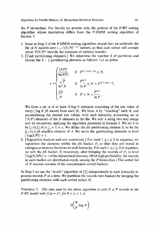
the P hierarchies. For brevity we present only the portion of the P-BT sorting algorithm whose description differs from the P-HMM sorting algorithm of Section 5.

2. Same as Step 2 of the P-HMM sorting algorithm, except that we subdivide the file of N records into t = F(N/P) 1 - ~ subsets, so that each subset will contain about P(N/Py records, for purposes of optimal transfer.

3. [Find partitioning elements.] We determine the number S of partitions and choose the S - 1 partitioning elements as follows: Let us define

( (NPy

ln(NP)

x - x/P

if p~1+~)/(1-~) < N,

p3/2 if - - < N < P( ~ + ~)/(1 - or)

In P

if p3/2

P < N < - - In P"

We form a set A of at least N/log N elements consisting of the key value of every [_log NAth record from each ~i. We form A by "touching" each ~i and accumulating the desired key values, with each hierarchy processing up to FN/P-] elements of the N elements in the file. We sort A using two-way merge sort by recursively applying the algorithm presented in Lemma 1. We set S to be [_IAI/[_lAr/x_J_J + 1 ~ x. We define the j th partitioning element bj to be the j[_[A[/xdth smallest element of A. We move the partitioning elements to level Flog(S/P)-] + 1.

8. [Reposition buckets and sort recursively.] For each 1 _< j _< S in sequence, we reposition the elements within the j th bucket ~ so that they are stored in contiguous memory locations in each hierarchy. For each 1 _< j _< S in sequence, we sort the jth bucket ~ recursively, after bringing the records of ~ to level Flog(N/SP)-] + 1 of the hierarchical memory. (With high probability, the records in each bucket are distributed evenly among the P hierarchies.) The sorted list of N records consists of the concatenated sorted buckets.

In Step 5 we use the " touch" algorithm of [2] independently in each hierarchy to process records P at a time. We partition the records into buckets by merging the partitioning elements with each sorted subset ~i.

THEOREM 7. The time used by the above algorithm to sort N >_ P records in the P-BT model with f (x) = x ~, for 0 < ~ < 1, is

log N)


with overwhelming probability. In particular, the probability that the number of I/Os used is more than l times the average is exponentially small in/(log/) log P.

PROOF. Let T(N) be the time used by this algorithm to sort a file of N records. For N _> Pt~ +,)/tl-,), the time needed in Step 2 to subdivide the set of N records, move the subsets to faster memory, and sort the subsets ffi is bounded by

N �9 N l - , N ~

The time for touching the f#i subsets and accumulating the N/log N elements of set A in Step 3 is O((N/P)log log(N/P)) [2]. Using Lemma 1, we can show that the time for the two-way merge sort used in Step 3 to sort n elements is O((n/P) log n(log log n + log P)). Since n ~ N/log N, the resulting time to find the S partitioning elements is O((N/P)(log log N + log P)). The method of choosing the partitioning elements guarantees that the size Nj of the j th bucket is at most 2N/S, for each 1 < j < S. By Lemma 1, the time needed to partition the file in Steps 5-7 is O(t(N/tP)(log log N + log P) + t(S/P) log log S) = O((N/P)(log log N + log P)). The data movement to reposition the buckets in Step 8 can be done by the same method used by the one-hierarchy algorithm [2], that is, by computing the generalized matrix transposition for each hierarchy independently; the time needed is thus O((N/P)Oog log(N/P)) 4) with high probability. The analysis in the companion paper [11] can be modified to show that with high probability the records in each bucket are distributed evenly over the P hierarchies, so that the time for sorting the buckets recursively in Step 8 is with high probability

T(Nj)+ O( N log log N), l <_j<_S

where Nj is the size of the j th bucket Sj, ~1 <_i<_s Nj = N, and Nj < 2N/S for each j. Hence, for N _ ptl +,)/(1-,), with high probability we have

T(N) = -p T P ~ + Z 1 < j <~ F(NP)~/In(NP) "]

T(Nj)

and Nj < 2N 1 -~P-" ln(NP) for each j. If N < P~I +,)/tx-,), there will be at most a constant number of applications of

Phase 1 and one application of Phase 2, each phase taking O((N/P) log N) time with high probability. The remaining subfiles will have size at most P and can be


sorted in the base memory level in O((N/P) log P) time with high probability. This yields as desired the time bound

T(N) = O log N

with high probability. The probability bounds follow from those derived in [11]. []

A lower bound of ta((N/P) log N) time for sorting with f (x) = x ~, for �89 < ~ < 1, follows from the well-known lower bound for sorting in a RAM under the comparison model of computation.

6.2. Other Access Cost Functions. Since the above algorithm is optimal for the access cost function f (x) = x 1/2, it is also optimal for f (x) = log x and f (x) = x ~, for 0 < ~ <�89

Now let us consider the access cost function f ( x ) = x ~, where ~ > 1. For N > P3/2/ln P, we sort by a simple application of divide-and-conquer two-way merge sort. The upper bound of Theorem 2 follows by using the algorithm of Lemma 1 for merging two sorted lists. If N < P3/2/ln P, we use the partitioning algorithm (Phase 2) with t = NIP.

When f (x) = x ~, ~ = 1, and N < P3/2/ln P, the cost for the data movement in Step 2 is O((N/P)log(N/P)), and the cost for the actual sorting in the base memory level is O((N/P) log P). The set A in Step 3 can be sorted by binary merge sort in O((N/P)log N) time. The permuting and data movement in Step 6 takes O((N/PXlog P + log(N/P))) = O((N/P) log N) time, and the transposition and permuting required in Step 7 takes O((N/P)(log P + log2(N/P))) time. The data movement to reposition the buckets in Step 8 can be done as noted earlier by the one-hierarchy algorithm [2], that is, by computing the generalized matrix transposition for each hierarchy independently; the time needed is O((N/P)(log2(N/P))) with high probability. The previous remarks given in the proof of Theorem 7 about the distribution properties of Phase 2 still apply. This gives us the resulting high probability sorting time bound of O((N/P)(log2(N/P) + log N)) for the case f (x) = x ", ~ = 1, as listed in Theorem 2.

For the case N < P3/2/ln P when f (x) = x ~, ct > 1, the above algorithm yields the time bound in Theorem 2 of O((N/P) ~ + (N/P) log N).

The ~((N/P)log N) terms in the lower bounds of Theorem 2 come from the comparison model of computation. The f~((N/P)log2(N/P)) term in the lower bound for the case f (x) = x ", ~ = 1, the f~((N/P) ~ + (N/P) log N) term in the lower bound for the case f (x) = x ", ~ > 1, follow from a parallelization of the P = 1 bounds in [2].

7. F F T in P-HMM. The P -HMM lower bounds proved in Theorems 4 and 5 for sorting apply also to the F F T computation. This follows immediately by

164 J.s. vitter and E. A. M. Shriver

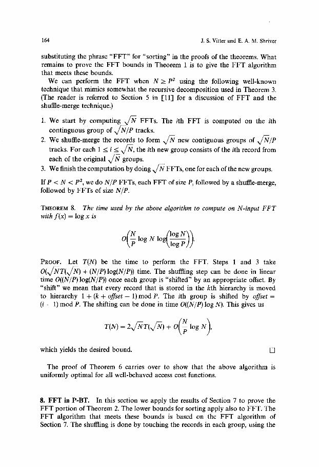
substituting the phrase " F F T " for "sorting" in the proofs of the theorems. What remains to prove the FFT bounds in Theorem 1 is to give the FFT algorithm that meets these bounds.

We can perform the FFT when N > p2 using the following well-known technique that mimics somewhat the recursive decomposition used in Theorem 3. (The reader is referred to Section 5 in 1-11] for a discussion of FFT and the shuffle-merge technique.)

1. We start by computing x /N FFTs. The ith FFT is computed on the ith

continguous group of a/NiP tracks.

2. We shuffle-merge the records to form x / ~ new contiguous groups of v/NiP tracks. For each 1 < i < ~ , the ith new group consists of the ith record from each of the original x / ~ groups.

3. We finish the computation by doing v /N FFTs, one for each of the new groups.

If P < N < p2, we do NiP FFTs, each FFT of size P, followed by a shuffle-merge, followed by FFTs of size NiP.

THEOREM 8. The time used by the above algorithm to compute on N-input FFT with f(x) = log x is

, t/log N'~'~

PROOF. Let T(N) be the time to perform the FFT. Steps 1 and 3 take

O(x//-NT(x/~ + (NIP)log(NiP)) time. The shuffling step can be done in linear time O((N/P)log(NiP)) once each group is "shifted" by an appropriate offset. By "shift" we mean that every record that is stored in the kth hierarchy is moved to hierarchy 1 + (k + offset- 1)rood P. The ith group is shifted by offset = (i - 1) mod P. The shifting can be done in time O((N/P) log N). This gives us

(N ) = + 0 F log N ,

which yields the desired bound. []

The proof of Theorem 6 carries over to show that the above algorithm is uniformly optimal for all well-behaved access cost functions.

8. FFT in P-BT. In this section we apply the results of Section 7 to prove the FFT portion of Theorem 2. The lower bounds for sorting apply also to FFT. The FFT algorithm that meets these bounds is based on the FFT algorithm of Section 7. The shuffling is done by touching the records in each group, using the


touching algorithm of [-2] applied to the hierarchies independently. For each P records of a group that are touched at the same time, the records are shifted by the offset amount while in the base level memory.

9. Standard Matrix Multiplication in P-HMM

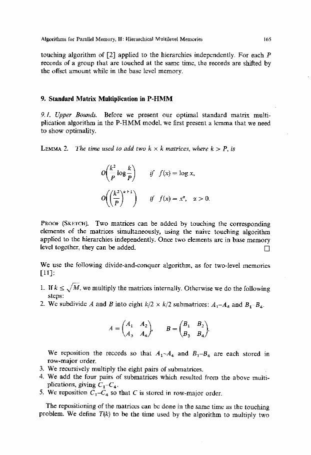
9.1. Upper Bounds. Before we present our optimal standard matrix multiplication algorithm in the P-HMM model, we first present a lemma that we need to show optimality.

LEMMA 2. The time used to add two k x k matrices, where k > P, is

k k ) O ~- log ff /f f (x) = log x,

{ { k2 "V<+ ix l

PROOF (SKETCH). Two matrices can be added by touching the corresponding elements of the matrices simultaneously, using the naive touching algorithm applied to the hierarchies independently. Once two elements are in base memory level together, they can be added. []

We use the following divide-and-conquer algorithm, as for two-level memories [11]:

1. If k < w/M, we multiply the matrices internally. Otherwise we do the following steps:

2. We subdivide A and B into eight k/2 x k/2 submatrices: Ax-A 4 and Bx-B 4.

A 3 A J ' B 3 B 4 "

We reposition the records so that A1-A 4 and B1-B 4 are each stored in row-major order.

3. We recursively multiply the eight pairs of submatrices. 4. We add the four pairs of submatrices which resulted from the above multi-

plications, giving C1-C 4. 5. We reposition C~-C 4 so that C is stored in row-major order.

The repositioning of the matrices can be done in the same time as the touching problem. We define T(k) to be the time used by the algorithm to multiply two


k x k matrices together. For f(x) = log x, we get from Lemma 2

Using the stopping condition T(x/rfi)= v/P, we get the desired upper bound O(k3/p) of Theorem 1. The upper bounds for the other access cost functions follow by using the other cases of Lemma 2.

9.2. Lower Bounds. The standard matrix multiplication algorithm given earlier for the logarithmic access cost is uniformly optimal, that is, it is optimal for all well-behaved access cost functions. This can be proved using the same approach as in Theorem 6. By [10], the I/O complexity of multipling two k x k matrices with one disk, no blocking, and an internal memory of size M is

(6) k3 ) Tu(k 2)=f~ ~ - M .

Let TM, p(N) be the average number of I/O steps done by the standard matrix multiplication algorithm with respect to an internal memory of size M, where we allow each hierarchy to move simultaneously, in a single I/O step, a record between

internal memory and external memory. From the algorithm, for k > x / ~ , we get the recurrence

TM,p(k) = 8T~t,p + ~ .

For smaller k < x ~ , we have TM,p(k ) = O(k/P). The solution of this recurrence is

T~t, e(k) = O

which by (6) is within an O(M/P) additive term of optimal. The time used by the algorithm in base memory level computations is

Therefore, the extra time used by the algorithm over and above the optimal amount is

(7) 0 + ~ ~ - 6 f = O + ~ f . P < M < k 2


The first term on the right-hand side of (7) is bounded by the number of operations performed, and the second term is the time required to access all the elements; thus the running time is within a constant factor of optimal.

10. Standard Matrix Multiplication in P-BT. Before we present the P-BT algorithm that yields the optimal bound quoted in Theorem 2 for standard matrix multiplication, we first present a useful lemma.

LEMMA 3. The time used to add two k x k matrices, where k > P, is

//k 2 k2Xx O ~ l o g * ~ ) /f f ( x ) : logx,

O log logk if f ( x ) = x ~', 0 < ~ < 1 ,

log 0 if f ( x ) = x ~, a = l ,

0 if f ( x ) = x ~, a > l .

PROOF (SKETCH). We apply the same approach as in Lemma 2. Two matrices can be added by touching the corresponding elements of the matrices simultaneously, using the touching algorithm of l-2] applied to the hierarchies independently. Once two elements are in base memory level together, they can be added. The resultant matrix moves to slower memory in the same manner as the two matrices being added moved to faster memory, only backward. []

Let us consider the access cost function f ( x )= x ", where 0 < a < 1. The algorithm presented in Section 9 can be adapted to run on the P-BT model. The repositioning of the matrices can be done in the same time as the touching problem. We define T(k) to be the time used by the algorithm to multiply two k • k matrices together. It is easy to see that

T(k)= 8 T ( ~ ) + O ( ~ log log k).

Using the stopping condition T(x/~ ) = x/~, we get the desired upper bound O(ka/P) of Theorem 2 for the access cost function f(x) = x ~, where 0 < a < 1. The lower bound of f~(ka/P) clearly holds since the number of operations performed is O(k3).


Since the above algorithm is optimal for the access cost function f ( x ) = x 1/2, it is also optimal for f ( x ) = log x. The upper bounds for the remaining cases of Theorem 2 follow by applying the other cases of Lemma 3. The lower bound for the access cost function f ( x ) = x ~, where ~ = 3 for the BT model [2] can be modified for the P-BT model. When �9 > ~- we get a lower bound of fl((k2/py) since that is the time needed to access the farthest elements in memory.

11. Conclusions. We have presented optimal hierarchical memory algorithms for sorting and matrix-related problems that take advantage of multiple hierarchies. The sorting algorithm is a randomized version of distribution sort, using the partitioning technique of the companion paper [11], which was developed for optimal sorting on two-level memories with parallel block transfer,

ADDENDUM. Recently an alternative two-level sorting algorithm that is both optimal and deterministic was developed by Nodine and Vitter [6]. The algorithm is based on merge sort and does not seem to provide optimal P-HMM and P-BT algorithms when applied to hierarchical memory. Subsequently, Nodine and Vitter developed optimal sorting algorithms for P-HMM and P-BT based on distribution sort that are deterministic [8].

Another interesting type of hierarchical memory is introduced in [4]. Parallel hierarchies of this type are studied in [7].

Acknowledgments. We thank Mark Nodine and Greg Plaxton for their helpful comments.

References

[1] A. Aggarwal, B. Alpern, A. K. Chandra, and M. Snir, A Model for Hierarchical Memory, Proceedings of the 19th Annual ACM Symposium on Theory of Computing, May 1987, pp. 305-314.

I-2] A. Aggarwal, A. Chandra, and M. Snir, Hierarchical Memory with Block Transfer, Proceedings of the 28th Annual IEEE Symposium on Foundations of Computer Science, October 1987, pp. 204-216.

I'3] A. Aggarwal and J. S. Vitter, The Input/Output Complexity of Sorting and Related Problems, Communications of the A CM 31(9) (September 1988), 1116-1127.

I-4] B. Alpern, L. Carter, E. Feig, and T. Selker, The Uniform Memory Hierarchy Model of Computation, Algorithmica, this issue, pp. 72-109.

1-5] F. Luccio and L Pagli, A Model of Sequential Computation Based on a Pipelined Access to Memory, Proceedings of the 27th Annual Allerton Conference on Communication, Control, and Computing, September 1989.

1-61 M.H. Nodine and J. S. Vitter, Large-Scale Sorting in Parallel Memories, Proceedings of the 3rd Annual ACM Symposium on Parallel Algorithms and Architectures, July 1991, pp. 29-39.

1-7] M.H. Nodine and J. S. Vitter, Large-Scale Sorting in Uniform Memory Hierarchies, Journal of Parallel and Distributed Computing (January 1993), special issue.


[8] M. H. Nodine and J. S. Vitter, Deterministic Distribution Sort in Shared and Distributed Memory Multiprocessors, Proceedings of the 5th Annual ACM Symposium on Parallel Algo- rithms and Architectures, July 1993, pp. 120-129.

[9] J.H. Reif and L. G. Valiant, A Logarithmic Time Sort on Linear Size Networks, Journal of the ACM 34 (January 1987), 60-76.

[10] J. Savage and J. S. Vitter, Parallelism in Space-Time Tradeoffs, in Advances in Computing Research, Vol. 4, F. P. Preparata, ed., JAI Press, Greenwich, CT 1987, pp. 117-146.

[11] J.S. Vitter and E. A. M. Shriver, Algorithms for Parallel Memory, I: Two-Level Memories, Algorithmica, this issue, pp. 110-147.

algorithms for parallel memory, ii: hierarchical multilevel

Documents