Algorithms for Probabilistically-Constrained Models ofRisk-Averse Stochastic Optimization with Black-Box Distributions

Chaitanya Swamy∗

Abstract

We consider various stochastic models that incorporate the notion of risk-averseness into the standard2-stage recourse model, and develop novel techniques for solving the algorithmic problems arising inthese models. A key notable feature of our work that distinguishes it from work in some other relatedmodels, such as the (standard) budget model and the (demand-) robust model, is that we obtain resultsin the black-box setting, that is, where one is given only sampling access to the underlying distribution.Our first model, which we call the risk-averse budget model, incorporates the notion of risk-aversenessvia a probabilistic constraint that restricts the probability (according to the underlying distribution) withwhich the second-stage cost may exceed a given budget B to at most a given input threshold ρ. We alsoa consider a closely-related model that we call the risk-averse robust model, where we seek to minimizethe first-stage cost and the (1− ρ)-quantile (according to the distribution) of the second-stage cost.

We obtain approximation algorithms for a variety of combinatorial optimization problems includingthe set cover, vertex cover, multicut on trees, min cut, and facility location problems, in the risk-aversebudget and robust models with black-box distributions. We first devise a fully polynomial approximationscheme for solving the LP-relaxations of a wide-variety of risk-averse budgeted problems. Complement-ing this, we give a rounding procedure that lets us use existing LP-based approximation algorithms forthe 2-stage stochastic and/or deterministic counterpart of the problem to round the fractional solution.Thus, we obtain near-optimal solutions to risk-averse problems that preserve the budget approximatelyand incur a small blow-up of the probability threshold (both of which are unavoidable). To the best ofour knowledge, these are the first approximation results for problems involving probabilistic constraintsand black-box distributions. Our results extend to the setting with non-uniform scenario-budgets, and toa generalization of the risk-averse robust model, where the goal is to minimize the sum of the first-stagecost and a weighted combination of the expectation and the (1− ρ)-quantile of the second-stage cost.

1 Introduction

Stochastic optimization models provide a means to model uncertainty in the input data where the uncertaintyis modeled by a probability distribution over the possible realizations of the actual data, called scenarios.Starting with the work of Dantzig [10] and Beale [2] in the 1950s, these models have found increasingapplication in a wide variety of areas; see, e.g., [4, 35] and the references therein. An important and widely-used model in stochastic programming is the 2-stage recourse model: first, given the underlying distributionover scenarios, one may take some first-stage actions to construct an anticipatory part of the solution, x,incurring an associated cost c(x). Then, a scenario A is realized according to the distribution, and onemay take additional second-stage recourse actions yA incurring a certain cost fA(x, yA). The goal in thestandard 2-stage model is to minimize the total expected cost, c(x) + EA

[fA(x, yA)

]. Many applications

come under this setting. An oft-cited motivating example is the 2-stage stochastic facility location problem.A company has to decide where to set up its facilities to serve client demands. The demand-pattern is not

∗cswamy@math.uwaterloo.ca. Dept. of Combinatorics and Optimization, Univ. Waterloo, Waterloo, ON N2L 3G1.Supported in part by NSERC grant 32760-06.

1

known precisely at the outset, but one does have some statistical information about the demands. The first-stage decisions consist of deciding which facilities to open initially, given the distributional informationabout the demands; once the client demands are realized according to this distribution, we can extend thesolution by opening more facilities, incurring their recourse costs. The recourse costs are usually higherthan the original ones (e.g., because opening a facility later involves deploying resources with a small leadtime), could be different for the different facilities, and could even depend on the realized scenario.

A common criticism of the standard 2-stage model is that the expectation measure fails to adequatelymeasure the “risk” associated with the first-stage decisions: two solutions with the same expected cost arevalued equally. But in realistic settings, one also considers the risk involved in the decision. For example, inthe stochastic facility location problem, given two solutions with the same expected cost, one which incurs amoderate second-stage cost in all scenarios, and one where there is a non-negligible probability that a “dis-aster scenario” with a huge associated cost occurs, a company would naturally prefer the former solution.

Our models and results. We consider various stochastic models that incorporate the notion of risk-averseness into the standard 2-stage model and develop novel techniques for solving the algorithmic prob-lems arising in these models. A key notable feature of our work that distinguishes it from work in some otherrelated models [19, 11], is that we obtain results in the black-box setting, that is, where one is given onlysampling access to the underlying distribution. To better motivate our models, we first give an overview ofsome related models considered in the approximation-algorithms literature that also embody the idea of risk-protection, and point out why these models are ill-suited to the design of algorithms in the black-box setting.

One simple and natural way of providing some assurance against the risk due to scenario-uncertainty isto provide bounds on the second-stage cost incurred in each scenario. Two closely related models in thisvein are the budget model, considered by Gupta, Ravi and Sinha [19], and the (demand-) robust model,considered by Dhamdhere, Goyal, Ravi and Singh [11]. In the budget model, one seeks to minimize theexpected total cost subject to the constraint that the second-stage cost fA(x, yA) incurred in every scenarioA be at most some input budget B. (In general, one could have a different budget BA for each scenario A,but for simplicity we focus on the uniform-budget model.) Gupta et al. considered the budget model in thepolynomial scenario setting, where one is given explicitly a list of all scenarios (with non-zero probability)and their probabilities, thereby restricting their attention to distributions with a polynomial-size support. Inthe robust model considered by Dhamdhere et al. [11], which is more in the spirit of robust optimization,the goal is to minimize c(x) + maxA fA(x, yA). It is easy to see how the two models are related: if one“guesses” the maximum second-stage cost B incurred by the optimum, then the robust problem essentiallyreduces to the budget problem with budget B, except that the second-stage cost term in the objective func-tion is replaced by B (which is a constant). Notice that it is not clear how to even specify problems withexponentially many scenarios in the robust model. Feige et al. [14] expanded the model of [11] by consid-ering exponentially many scenarios, where the scenarios are implicitly specified by a cardinality constraint.However, considering scenario-collections that are determined only by a cardinality constraint seems ratherspecialized and somewhat artificial, especially in the context of stochastic optimization; e.g., in facility loca-tion, it is rather stylized (and overly conservative) to assume that every set of k clients (for some k) may showup in the second-stage. We will consider a more general way of specifying (exponentially many) scenariosin robust problems, where the input specifies a black-box distribution and the collection of scenarios is thengiven by the support of this distribution. We shall call this model the distribution-based robust-model.

Both the budget model and the (distribution-based) robust model suffer from certain common drawbacks.A serious algorithmic limitation of both these models (see Section 5) is that for almost any (non-trivial)stochastic problem (such as fractional stochastic set cover with at most 3 elements, 3 sets, 3 scenarios), onecannot obtain any approximation guarantees in the black-box setting using any bounded number of samples(even allowing for a bounded violation of the budget in the budget model). Intuitively, the reason forthis is that there could be scenarios that occur with vanishingly small probability that one will almost never

2

encounter in our samples, but which essentially force one to take certain first-stage actions in order to satisfythe budget constraints in the budget model, or to obtain a low-cost solution in the robust model. Notice alsothat both the budget and robust models adopt the conservative view that one needs to bound the second-stage cost in every scenario, regardless of how likely it is for the scenario to occur. (By the same token,they also provide the greatest amount of risk-aversion.) In contrast, many of the risk-models consideredin the finance and stochastic-optimization literature, such as the mean-risk model [27], value-at-risk (VaR)constraints [30, 23, 32], conditional VaR [34], do factor in the probabilities of different scenarios.

Our models for risk-averse stochastic optimization address the above issues, and significantly refineand extend the budget and robust models. Our goal is to come up with a model that is sufficiently rich inmodeling power to allow for black-box distributions, and in which one can obtain strong algorithmic results.Our models are motivated by the observation (see Appendix A) that it is possible to obtain approximationguarantees in the budget model with black-box distributions, if one allows the second-stage cost to exceedthe budget with some “small” probability ρ (according to the underlying distribution). We can turn thissolution concept around and incorporate it into the model to arrive at the following. We are now given aprobability threshold ρ ∈ [0, 1]. In our new budget model, which we call the risk-averse budget model,given a budget B, we seek (x, yA) so as to minimize c(x) + EA

[fA(x, yA)

]subject to the probabilistic

constraint PrA[fA(x, yA) > B] ≤ ρ. The corresponding risk-averse (distribution-based) robust modelseeks to minimize c(x) +Qρ[fA(x, yA)], where Qρ[fA(x, yA)] is the (1− ρ)-quantile of fA(x, yA)A∈A,which is the smallest number B such that PrA[fA(x) > B] ≤ ρ. Notice that the parameter ρ allows usto control the risk-aversion level and tradeoff risk-averseness against conservatism (in the spirit of [3, 41]).Taking ρ = 1 in the risk-averse budget model gives the standard 2-stage recourse model, whereas taking ρ =0 in the risk-averse budget- or robust-models recovers the standard budget- and robust models respectively.In the sequel, we treat ρ as a constant that is not part of the input.

We obtain approximation algorithms for a variety of combinatorial optimization problems (Section 4)including the set cover, vertex cover, multicut on trees, min cut, and facility location problems, in therisk-averse budget and robust models with black-box distributions. We obtain near-optimal solutions thatpreserve the budget approximately and incur a small blow-up of the probability threshold. (One shouldexpect to violate the budget here; otherwise, by setting very high first-stage costs, one would be able to solvethe decision version of an NP-hard problem!) To the best of our knowledge, these are the first approximationresults for problems with probabilistic constraints and black-box distributions. Our results extend to thesetting with non-uniform scenario-budgets, and to a generalization of the risk-averse robust model, wherethe goal is to minimize c(x) plus a weighted combination of EA

[fA(x, yA)

]and Qρ[fA(x, yA)]. In the

sequel, we focus primarily on the risk-averse budget model since results obtained this model essentiallytranslate to the risk-averse robust model (the budget-violation can be absorbed into the approximation ratio).

Our results are built on two components. First, and this is the technically more difficult component andour main contribution, we devise a fully polynomial approximation scheme for solving the LP-relaxationsof a wide-variety of risk-averse problems (Theorem 3.3). We show that in the black-box setting, for a widevariety of 2-stage problems, for any ε, κ > 0, in time poly

(λ

εκρ

), one can compute (with high probability) a

solution to the LP-relaxation of the risk-averse budgeted problem, of cost at most (1+ ε) times the optimumwhere the probability that the second-stage cost exceeds the budgetB is at most ρ(1+κ). Here λ is the max-imum ratio between the costs of the same action in stage II and stage I (e.g., opening a facility or choosing aset). We show in Section 5 that the dependence on 1

κρ , and hence, the violation of the probability-threshold,is unavoidable in the black-box setting. We believe that this is a general tool of independent interest thatwill find application in the design of approximation algorithms for other discrete risk-averse stochastic op-timization problems, and that our techniques will find use in solving other probabilistic programs.

The second component is a simple rounding procedure (Theorem 3.2) that complements (and motivates)the above approximation scheme. As we mention below, our LP-relaxation is a relaxation of even thefractional risk-averse problem (i.e., where one is allowed to take fractional decisions). We give a general

3

rounding procedure to convert a solution to our LP-relaxation to a solution to the fractional risk-averseproblem losing a certain factor in the solution cost, budget, and the probability of budget-violation. Thisallows us to then use an LP-based “local” approximation algorithm for the corresponding 2-stage problem toobtain an integer solution, where a local algorithm is one that approximately preserves the LP-cost of eachscenario. In particular, for various covering problems, one can use the local 2c-approximation algorithmin [38], which is obtained using an LP-based c-approximation algorithm for the deterministic problem.

We need to overcome various obstacles to devise our approximation scheme. The first difficulty facedin solving a probabilistic program such as ours, is that the feasible region of even the fractional problemis a non-convex set. Thus, even in the polynomial-scenario setting, it is not clear how to solve (even) thefractional risk-averse problem. (In contrast, in the standard 2-stage recourse model, the fractional problemcan be easily formulated and solved as a linear program (LP) in the polynomial-scenario setting.) Weformulate an LP-relaxation (which is also a relaxation of the fractional problem), where we introduce avariable rA for every scenario A that is supposed to indicate whether the budget is exceeded in scenarioA. Correspondingly, we have two sets of decision variables to denote the decisions taken in scenario Ain the two cases respectively where the budget is exceeded and where it is not exceeded. The constraintsthat enforce this semantics will of course be problem-specific, but a common constraint that figures in allthese formulations is

∑A pArA ≤ ρ, which captures our probabilistic constraint. This constraint, which

couples the different scenarios, creates significant challenges in solving the LP-relaxation. (Again, noticethe contrast with the standard 2-stage recourse model.) We get around the difficulty posed by this couplingconstraint by taking the Lagrangian dual with respect to this constraint, introducing a dual variable ∆ ≥ 0.The resulting maximization problem (over ∆) has a 2-stage minimization LP embedded inside it. Althoughthis 2-stage LP does not belong to the class of problems defined in [38, 45, 7], we prove that for any fixed ∆,this 2-stage LP can be solved to “near-optimality” using the sample average approximation (SAA) method.The crucial insight here is to realize that for the purpose of obtaining a near-optimal solution to the risk-averse LP, it suffices to obtain a rather weak guarantee for the 2-stage LP, where we allow for an additiveerror proportional to ∆. This guarantee is specifically tailored so that it is weak enough that one can provesuch a guarantee by showing “closeness-in-subgradients” and the analysis in [45], and yet can be leveragedto obtain a near-optimal solution to (the relaxation of) our risk-averse problem. Given this guarantee, weshow that one can efficiently find a suitable value for ∆ such that the solution obtained for this ∆ (via theSAA method) satisfies the desired guarantees.

Related work. Stochastic optimization is a field with a vast amount of literature; we direct the reader to [4,30, 35] for more information on the subject. We survey the work that is most relevant to our work. Stochasticoptimization problems have only recently been studied from an approximation-algorithms perspective. Avariety of approximation results have been obtained in the 2-stage recourse model, but more general models,such as risk-optimization or probabilistic-programming models have received little or no attention.

The (standard) budget model was first considered by Gupta et al. [19], who designed approximationalgorithms for stochastic network design problems in this model. Dhamdhere et al. [11] introduced thedemand-robust model (which we call the robust model), and obtained algorithms for the robust versions ofvarious combinatorial optimization problems; some of their guarantees were later improved by Golovin etal. [16]. All these works focus on the polynomial-scenario setting. Feige, Jain, Mahdian, and Mirrokni [14]considered the robust model with exponentially many scenarios that are specified implicitly via a cardinalityconstraint, and derived approximation algorithms for various covering problems in this more general model.

There is a large body of work in the finance and stochastic-optimization literature, dating back toMarkowitz [27], that deals with risk-modeling and optimization; see e.g., [34, 1, 36] and the referencestherein. Our risk-averse models are related to some models in finance. In fact, the probabilistic constraintthat we use is called a value-at-risk (VaR) constraint in the finance literature, and its use in risk-optimizationis quite popular in finance models; it has even been written into some industry regulations [23, 32].

4

Problems involving probabilistic constraints are called probabilistic or chance-constrained programs [8,29] in the stochastic-optimization literature, and have been extensively studied (see, e.g., Prekopa [31]). Re-cent work in this area [6, 28, 13] has focused on replacing the original probabilistic constraint by moretractable constraints so that any solution satisfying the new constraints also satisfies the original probabilis-tic constraint with high probability. Notice that this type of “relaxation” is opposite to what one aims forin the design of approximation algorithms, where we want that every solution to the original problem re-mains a solution to the relaxation (but most likely, not vice versa). Although some approximation resultsin the opposite direction are obtained in [6, 28, 13], they are obtained for very structured constraints ofthe type Prξ[G(x, ξ) /∈ C] ≤ ρ, where C is a convex set, ξ is a continuous random variable whose dis-tribution satisfies a certain concentration-of-measure property, and G(.) is a bi-affine or convex mapping;also the bounds obtained involve a relatively large violation of the probability threshold (compared to our(1 + κ)-factor). To the best of our knowledge, there is no prior work in the stochastic-optimization orfinance literature on the design of efficient algorithms with provable worst-case guarantees for discrete risk-optimization or probabilistic-programming problems. In the Computer Science literature, [24] and [15]consider the stochastic bin packing and knapsack problems with probabilistic constraints that limit the over-flow probability of a bin or the knapsack, and obtained novel approximation algorithms for these problems.Their results are however obtained for specialized distributions where the item sizes are independent randomvariables following Bernoulli, exponential, or Poisson distributions specified in the input. In the context ofstochastic optimization, this constitutes a rather stylized setting that is far from the black-box setting.

The work closest in spirit to ours is that of So, Zhang, and Ye [41]. They consider the problem ofminimizing the first-stage cost plus a risk-measure called the conditional VaR (CVaR) [34]. Their modelinterpolates between the 2-stage recourse model and the (standard) robust model (as opposed to the budgetmodel in our case). They give an approximation scheme for solving the LP-relaxations of a broad class ofproblems in the black-box setting, using which they obtain approximation algorithms for certain discreteoptimization problems. Our methods are however quite different from theirs. In their model, the fractionalproblem yields a convex program and moreover, they are able to use a nice representation theorem in [34]for the CVaR measure to convert their problem into a 2-stage problem and then adapt the methods in [7].In our case, the non-convexity inherent in the probabilistic constraint creates various difficulties (first thenon-convexity, then the coupling constraint) and we consequently need to work harder to obtain our result.We remark that our techniques can be used to solve a generalization of their model, where we have the sameobjective function but also include a probabilistic budget constraint as in our risk-averse budget model.

We now briefly survey the approximation results in recourse models. The first such approximation re-sult appears to be due to Dye, Stougie, and Tomasgard [12]. The recent interest and flurry of algorithmicactivity in this area can be traced to the work of Ravi and Sinha [33] and Immorlica, Karger, Minkoff andMirrokni [22], which gave approximation algorithms for the 2-stage variants of various discrete optimiza-tion problems in the polynomial scenario [33, 22] and independent-activation [22] settings. Approximationalgorithms for 2-stage problems with black-box distributions were first obtained by Gupta, Pal, Ravi andSinha [17], and subsequently by Shmoys and Swamy [38] (see also preliminary version [39]). Various otherapproximation results for 2-stage problems have since been obtained; see, e.g., the survey [44]. Multi-stage recourse problems in the black-box model were considered by [18, 45]; both obtain approximationalgorithms with guarantees that deteriorate with the number of stages, either exponentially [18] (except formultistage Steiner tree which was also considered in [20]), or linearly [45]; improved guarantees for setcover and vertex cover have been subsequently obtained [42].

Our approximation scheme makes use of the SAA method, which is a simple and appealing method forsolving stochastic problems that is quite often used in practice. In the SAA method one samples a certainnumber of scenarios to estimate the scenario probabilities by their frequency of occurrence, and then solvesthe 2-stage problem determined by this approximate distribution. The effectiveness of this method dependson the sample size (ideally, polynomial) required to guarantee that an optimal solution to the SAA-problem

5

is a provably near-optimal solution to the original problem. Kleywegt et al. [25] (see also [37]) prove a boundthat depends on the variance of a certain quantity that need not be polynomially bounded. Subsequently,Swamy and Shmoys [45], and Charikar et al. [7] obtained improved (polynomial) sample-bounds for a largeclass of structured 2-stage problems. The proof in [45], which also applies to multistage programs, is basedon leveraging approximate subgradients, and our proof makes use of portions of their analysis. The proof ofCharikar et al. [7] is quite different; it applies to 2-stage programs but proves the stronger theorem that evenapproximate solutions to the SAA problem translate to approximate solutions to the original problem.

2 Preliminaries

Let R+ denote R≥0. Let ‖u‖ denote the `2 norm of u. The Lipschitz constant of a function f : Rm 7→ Ris the smallest K such that |f(x) − f(y)| ≤ K‖x − y‖. We consider convex minimization problemsminx∈P f(x), where P ⊆ Rm

+ with P ⊆ B(0, R) = x : ‖x‖ ≤ R for a suitable R, and f is convex.

Definition 2.1 Let f : Rm 7→ R be a function. We say that d ∈ Rm is a subgradient of f at the point u ifthe inequality f(v)− f(u) ≥ d · (v − u) holds for every v ∈ Rm. We say that d is an (ω, ξ)-subgradient off at the point u ∈ P if for every v ∈ P , we have f(v)− f(u) ≥ d · (v − u)− ωf(v)− ωf(u)− ξ.

The above definition of an (ω, ξ)-subgradient is slightly weaker than the notion of an ω-subgradient asdefined in [38], where one requires that f(v)−f(u) ≥ d ·(v−u)−ωf(u). But this difference is superficial;one could also implement the algorithm in [38] using the weaker notion of an (ω, ξ)-subgradient. It is wellknown (see [5]) that a convex function has a subgradient at every point. One can infer from Definition 2.1that, letting dx denote a subgradient of f at x, the Lipschitz constant of f is at most maxx ‖dx‖.

Let K be a positive number, and τ, % be two parameters with τ < 1. Let N = log(

2KRτ

). Let G′τ ⊆ P

be a discrete set such that for any x ∈ P , there exists x′ ∈ G′τ with ‖x − x′‖ ≤ τKN . Define Gτ =

G′τ ∪x + t(y − x), y + t(x − y) : x, y ∈ G′τ , t = 2−i, i = 1, . . . , N

. We call Gτ and G′τ , an τ

KN -netand an extended τ

KN -net respectively of P . As shown in [45], if P contains a ball of radius V (where V ≤ 1without loss of generality), then one can construct G′τ so that |Gτ | = poly

(log(KR

V τ )). As mentioned earlier,

our algorithms make use of the sample average approximation (SAA) method. The following result fromSwamy and Shmoys [45], which we have adapted to our setting, will be our main tool for analyzing theSAA method.

Lemma 2.2 ([45]) Let f and f be two nonnegative convex functions with Lipschitz constant at mostK suchthat at every point x ∈ Gτ , there exists a vector dx ∈ Rm that is a subgradient of f(.) and an

( %8N , ξ

)-

subgradient of f(.) at x. Let x = argminx∈P f(x). Then, f(x) ≤ (1 + %) minx∈P f(x) + 6τ + 2Nξ.

Lemma 2.3 (Chernoff-Hoeffding bound [21]) LetX1, . . . , XN be iid random variables with eachXi ∈ [0, 1]and µ = E

[Xi

]. Then, Pr[

∣∣ 1N

∑iXi − µ

∣∣ > ε] ≤ 2e−2ε2N .

3 The risk-averse budgeted set cover problem: an illustrative example

Our techniques can be used to efficiently solve the risk-averse versions of a variety of 2-stage stochasticoptimization problems, both in the risk-averse budget and robust models. In this section, we illustrate themain underlying ideas by focusing on the risk-averse budgeted set cover problem. In the risk averse budgetedset cover problem (RASC), we are given a universe U of n elements and a collection S of m subsets of U .The set of elements to be covered is uncertain: we are given a probability distribution pAA∈A of scenarios,where each scenarioA specifies a subset ofU to be covered. The cost of picking a set S ∈ S in the first-stageis wI

S , and is wAS in scenario A. The goal is to determine which sets to pick in stage I and which ones to pick

6

in each scenario so as to minimize the expected cost of picking sets, subject to PrA[cost of scenario A >B] ≤ ρ, where ρ is a constant that is not part of the input. Notice that the costs wA

S are only revealed whenwe sample scenario A; thus, the “input size”, denoted by I is O(m+ n+

∑S logwS + logB).

For a given (fractional) point x ∈ Rm with 0 ≤ xS ≤ 1 for all S, define fA(x) to be the minimum valueof wA ·yA subject to

∑S:e∈S yA,S ≥ 1−

∑S:e∈S xS for e ∈ A, and yA,S ≥ 0 for all S. Let P = [0, 1]m. As

mentioned in the Introduction, the set of feasible solutions to even the fractional risk-averse problem (whereone can buy sets fractionally) is not in general a convex set. We consider the following LP-relaxation of theproblem, which is a relaxation of even the fractional risk-averse problem (Claim 3.1). Throughout we useA to index the scenarios in A, and S to index the sets in S.

min∑S

wISxS +

∑A,S

pA

(wA

S yA,S + wAS zA,S

)(RASC-P)

s.t.∑A

pArA ≤ ρ (1)∑S:e∈S

(xS + yA,S

)+ rA ≥ 1 for all A, e ∈ A, (2)∑

S:e∈S

(xS + yA,S + zA,S

)≥ 1 for all A, e ∈ A, (3)∑

S

wAS yA,S ≤ B for all A (4)

xS , yA,S , zA,S , rA ≥ 0 for all A,S. (5)

Here x denotes the first-stage decisions. The variable rA denotes whether one exceeds the budget of Bfor scenario A, and the variables yA,S and zA,S denote respectively the sets picked in scenario A in thesituations where one does not exceed the budget (so rA = 0) and where one does exceed the budget (sorA = 1). Consequently, constraint (4) ensures that the cost of the yA decisions does not exceed the budgetB, and (1) ensures that the total probability mass of scenarios where one does exceed the budget is at mostρ. Let OPT denote the optimum value of (RASC-P).

A significant difficulty faced in solving (RASC-P) is that the scenarios are no longer separable given afirst-stage solution, since constraint (1) couples the different scenarios. As a consequence, in order to specifya solution to (RASC-P) one needs to compute a first-stage solution and give an explicit procedure thatcomputes (yA, zA, rA) in any given scenario A. In our algorithms however, we can avoid this complicationbecause, as we show below, given only the first-stage component of a solution to (RASC-P), one can roundit to a first-stage solution to the fractional risk-averse problem (and then to an integer solution) losing a smallfactor in the solution cost and the probability-threshold. But observe that if we have a first-stage solution x tothe fractional risk-averse problem with probability-threshold P such that there exist second-stage solutionsyielding a total expected cost of C, then one can also easily compute second-stage solutions that yield nogreater total cost (and where Pr[second-stage cost > B] ≤ P ), by simply solving the LP fA(x) in eachscenario A. This implies that our algorithm for solving (RASC-P) only needs to return a first-stage solutionto (RASC-P) that can be extended to a near-optimum solution (without specifying an explicit procedure tocompute the second-stage solutions).

We show (Theorem 3.3) that for any ε, κ > 0, one can efficiently compute a first-stage solution x forwhich there exist solutions (yA, zA, rA) in every scenario A satisfying (2)–(5) such that wI ·x+

∑A pAw

A ·(yA + zA) ≤ (1 + 2ε)OPT , and

∑A pArA ≤ ρ(1 + κ). Complementing this, we give a simple rounding

procedure based on the rounding theorem in [38] to convert a fractional solution to (RASC-P) to an integersolution using an LP-based c-approximation algorithm for the deterministic set cover (DSC) problem, thatis, an algorithm that returns a set cover of cost at most c times the optimum of the standard LP-relaxationfor DSC. We prove this rounding theorem first, in order to better motivate our goal of solving (RASC-P).

7

Claim 3.1 OPT is a lower bound on the optimum of the fractional risk-averse problem.

Proof : We show that any solution x to the fractional risk-averse problem can be mapped to a solutionto (RASC-P) of no greater cost. Let yA be such that fA(x) = wA · yA, so Pr[fA(x) > B] ≤ ρ. Weset x = x. For scenario A, if fA(x) ≤ B, we set rA = 0, yA = yA, zA = 0. Otherwise, we setrA = 1, yA = 0, zA = yA. It is easy to see that this yields a feasible solution to (RASC-P) of costwI · x+

∑A pAfA(x).

Theorem 3.2 (Rounding theorem) Let(x, (yA, zA, rA)

)be a solution satisfying (2)–(5) of objective

value C =(wA · x+

∑A pAw

A · (yA + zA)), and let P =

∑A pArA. Given any ε > 0, one can obtain

(i) a solution x such that wI · x+∑

A pAfA(x) ≤(1 + 1

ε

)C and PrA

[fA(x) > (1 + 1

ε )B]≤ (1 + ε)P ;

(ii) an integer solution (x, yA) of cost at most 2c(1 + 1

ε

)C such that PrA

[wA · yA > 2cB(1 + 1

ε )]≤

(1 + ε)P using an LP-based c-approximation algorithm for the deterministic set cover problem.

Moreover, one only needs to know the first-stage solution x to obtain x and x.

Proof : Set x =(1 + 1

ε

)x. Consider any scenario A. Observe that (yA + zA) yields a feasible solution to

the second-stage problem for scenario A. Also, if rA < 11+ε , then

(1 + 1

ε

)yA also yields a feasible solution.

Thus, we have fA(x) ≤ wA · (yA + zA) and if rA < 11+ε then we also have fA(x) ≤

(1 + 1

ε

)B. So

wI · x+∑

A pAfA(x) ≤(1 + 1

ε

)C and Pr

[fA(x) > (1 + 1

ε )B]≤

∑A:rA≥ 1

1+εpA ≤ (1 + ε)P .

We can now round x to an integer solution (x, yA) using the Shmoys-Swamy [38] rounding procedure(which only needs x) losing a factor of 2c in the first- and second-stage costs. This proves part (ii).

3.1 Solving the risk-averse problem (RASC-P)

We now describe and analyze the procedure used to solve (RASC-P). First, we get around the difficultyposed by the coupling constraint (1) in formulation (RASC-P) by using the technique of Lagrangian relax-ation. We take the Lagrangian dual of (1) introducing a dual variable ∆ to obtain the following formulation.

max∆≥0

−∆ρ+(minx∈P

h(∆;x) = wI · x+∑A

pAgA(∆;x))

(LD1)

where gA(∆;x) = min∑S

wAS

(yA,S + zA,S

)+ ∆rA s.t. (2)–(4), yA,S , zA,S , rA ≥ 0 for all S. (P)

It is straightforward to show via duality theory that (RASC-P) and (LD1) have the same optimal value, andmoreover that if (x∗, y∗A, z∗A, r∗A) is an optimal solution to (RASC-P) and ∆∗ is the optimal valuefor the dual variable corresponding to (1) then

(∆∗;x∗, (y∗A, z∗A, r∗A)

)is an optimal solution to (LD1).

Recall that P = [0, 1]m. Let OPT (∆) = minx∈P h(∆;x). So OPT = max∆≥0

(OPT (∆) − ∆ρ

). Let

λ = max1,maxA,S(wA

S /wIS)

, which we assume is known. The main result of this section is as follows.

Throughout, when we say “with high probability”, we mean that a failure probability of δ can be ensuredusing poly

(ln(1

δ ))-dependence on the sample size (or running time).

Theorem 3.3 For any ε, γ, κ > 0, RiskAlg (see Fig. 1) runs in time poly(I, λ

εκρ , log( 1γ )

), and returns with

high probability a first-stage solution x and solutions (yA, zA, rA) for each scenario A that satisfy (2)–(5)and such that (i) wI · x +

∑A pAw

A · (yA + zA) ≤ (1 + ε)OPT + γ; and (ii)∑

A pArA ≤ ρ(1 + κ).Under the very mild assumption (∗) that wI · x+ fA(x) ≥ 1 for every A 6= ∅, x ∈ P ,1 we can convert thisguarantee into a (1 + 2ε)-multiplicative guarantee in the cost in time poly

(I, λ

εκρ

).

1A similar assumption is made in [38] to obtain a multiplicative guarantee.

8

RiskAlg (ε, γ, κ) [ε ≤ κ < 1; the quantities p(i), cost (i), (yA, zA, rA) are used only in the analysis.]

C1. Fix ε = ε/6, ζ = γ/4, η = ρκ/16. Also, set σ = ε/6, γ′ = γ/4, β = κ/8, and ρ′ = ρ(1 + 3κ/4).Consider the ∆ values ∆0,∆1, . . . ,∆k, where ∆0 = γ′, ∆i+1 = ∆i(1 + σ) and k is the smallest value suchthat ∆0(1 + σ)k ≥ UB. Note that k = O

(log(UB

γ′ )/σ).

C2. For each ∆i, let(x(i), (y(i)

A , z(i)A , r

(i)A )

)← SA-Alg(∆; ε, η, ζ) (here (y(i)

A , z(i)A , r

(i)A ) is an optimal solution to

gA(∆i;x(i)) and is implicitly given). Let p(i) =∑

A pAr(i)A and cost (i) = h(∆i;x(i)) = wI ·x(i)+

∑A pA

(wA ·

(y(i)A + z

(i)A ) + ∆ir

(i)A

).

C3. By sampling n = 12β2ρ2 ln

(4kδ

)scenarios, for each i = 0, . . . , k, compute an estimate p′(i) =

∑A qAr

(i)A of p(i),

where qA is the frequency of scenario A in the sampled set.

C4. If p′(0) ≤ ρ′ then return x(0) as the first-stage solution. [In scenario A, return (yA, zA, rA) = (y(0)A , z

(0)A , r

(0)A )].

C5. Otherwise (i.e., p′(0) > ρ′) find an index i such that p′(i) ≥ ρ′ and p′(i+1) ≤ ρ′ (we argue that such an i mustexist). Let a be such that a·p′(i)+(1−a)p′(i+1) = ρ′. Return the first-stage solution x = a·x(i)+(1−a)x(i+1).[In scenario A, return the solution (yA, zA, rA) = a(y(i)

A , z(i)A , r

(i)A ) + (1− a)(y(i+1)

A , z(i+1)A , r

(i+1)A ).]

SA-Alg (∆; ε, η, ζ) [K is (a bound on) the Lipschitz constant of h(∆; .); P ⊆ B(0, R) and P contains a ball ofradius V ≤ 1.]

B1. Set τ = ζ/6, N = log(

2KRV τ

). Let Gτ ⊆ P be an extended τ

KN -net of P as defined in Section 2, so that |Gτ | =poly

(log(KR

V τ )). Draw N = 8N2

(4λε + m

η

)2 ln( 2|Gτ |m

δ

)samples and for each scenario A, set pA = NA/N ,

where NA is the number of times scenario A is sampled.

B2. Solve the SAA problem minx∈P h(∆;x), where h(∆;x) = wI · x +∑

A pAgA(∆;x) to obtain a solution x.Return x and in scenario A, return the optimal solution to gA(∆; x).

Figure 1: The procedures RiskAlg and SA-Alg.

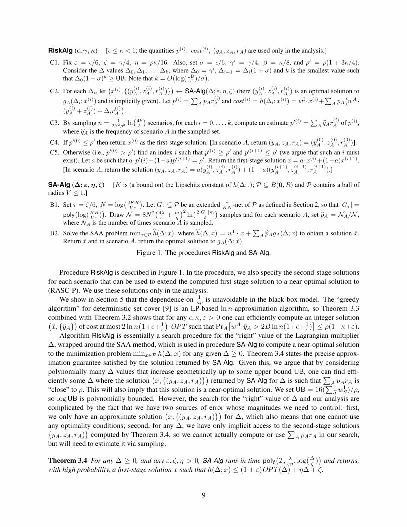
Procedure RiskAlg is described in Figure 1. In the procedure, we also specify the second-stage solutionsfor each scenario that can be used to extend the computed first-stage solution to a near-optimal solution to(RASC-P). We use these solutions only in the analysis.

We show in Section 5 that the dependence on 1κρ is unavoidable in the black-box model. The “greedy

algorithm” for deterministic set cover [9] is an LP-based lnn-approximation algorithm, so Theorem 3.3combined with Theorem 3.2 shows that for any ε, κ, ε > 0 one can efficiently compute an integer solution(x, yA

)of cost at most 2 lnn

(1+ε+ 1

ε

)·OPT such that PrA

[wA·yA > 2B lnn(1+ε+ 1

ε )]≤ ρ(1+κ+ε).

Algorithm RiskAlg is essentially a search procedure for the “right” value of the Lagrangian multiplier∆, wrapped around the SAA method, which is used in procedure SA-Alg to compute a near-optimal solutionto the minimization problem minx∈P h(∆;x) for any given ∆ ≥ 0. Theorem 3.4 states the precise approx-imation guarantee satisfied by the solution returned by SA-Alg. Given this, we argue that by consideringpolynomially many ∆ values that increase geometrically up to some upper bound UB, one can find effi-ciently some ∆ where the solution

(x, (yA, zA, rA)

)returned by SA-Alg for ∆ is such that

∑A pArA is

“close” to ρ. This will also imply that this solution is a near-optimal solution. We set UB = 16(∑

S wIS)/ρ,

so log UB is polynomially bounded. However, the search for the “right” value of ∆ and our analysis arecomplicated by the fact that we have two sources of error whose magnitudes we need to control: first,we only have an approximate solution

(x, (yA, zA, rA)

)for ∆, which also means that one cannot use

any optimality conditions; second, for any ∆, we have only implicit access to the second-stage solutionsyA, zA, rA) computed by Theorem 3.4, so we cannot actually compute or use

∑A pArA in our search,

but will need to estimate it via sampling.

Theorem 3.4 For any ∆ ≥ 0, and any ε, ζ, η > 0, SA-Alg runs in time poly(I, λ

εη , log(∆ζ )

)and returns,

with high probability, a first-stage solution x such that h(∆;x) ≤ (1 + ε)OPT (∆) + η∆ + ζ.

9

Analysis. For the rest of this section, ε, γ, κ are fixed values given by Theorem 3.3. We may assumewithout loss of generality that ε ≤ κ < 1. We prove Theorem 3.4 in Section 3.1.1. Here, we show how thisleads to the proof of Theorem 3.3. Given Theorem 3.4 and Lemma 2.3, we assume that the high probabilityevent “∀i, cost (i) ≤ (1 + ε)OPT (∆i) + η∆i + ζ and |p′(i) − p(i)| ≤ βρ” happens.

Claim 3.5 We have p(k) < ρ/2 and p′(k) < ρ/2.

Proof : If p(k) > ρ(1+ε)4 , then cost (k) − η∆k > 2(1 + ε)(

∑S w

IS) > (1 + ε)OPT (∆k) + ζ, which is a

contradiction. The last inequality follows since OPT (∆) ≤∑

S wIS for any ∆. Therefore, p(k) < ρ/2, and

p′(k) ≤ p(k) + βρ < ρ/2.

Proof of Theorem 3.3 : Let x be the first-stage solution returned by RiskAlg, and (yA, zA, rA) be thesolution returned for scenario A. It is clear that (2)–(5) are satisfied. Suppose first that p′(0) ≤ ρ′ (sox = x(0).) Part (ii) of the theorem follows since p(0) ≤ p′(0) + βρ ≤ ρ(1 + κ). Part (i) follows since

wI ·x(0)+∑A

pAwA ·(y(0)

A +z(0)A ) ≤ h(γ′;x) ≤ (1+ε)OPT (γ′)+ηγ′+ζ ≤ (1+ε)OPT +γ′(1+ε+η)+ζ.

The penultimate inequality follows because for any ∆, we have OPT (∆) ≤ OPT (0) + ∆ ≤ OPT + ∆.Now suppose that p′(0) > ρ′. In this case, there must exist an i such that p′(i) ≥ ρ′, and p′(i+1) ≤ ρ′

because p′(0) > ρ′ and p′(k) < ρ′ (by Claim 3.5), so step C4 is well defined. We again prove part (ii) first.We have

∑A pArA = a · p(i) + (1 − a)p(i+1) ≤ ρ′ + βρ ≤ ρ(1 + κ). To prove part (i), observe that

wI · x+∑

A pAwA · (yA + zA) ≤ a · cost (i) + (1− a) · cost (i+1) −∆i

(a · p(i) + (1− a) · p(i+1)

), which

is at most

(1 + ε)(a ·OPT (∆i) + (1− a)OPT (∆i+1)

)+ η(a∆i + (1− a)∆i+1) + ζ −∆i(ρ′ − βρ).

Now noting that ∆i+1 = (1 + σ)∆i, it is easy to see that OPT (∆i+1) ≤ (1 + σ)OPT (∆i). Also,ρ′−βρ−η(1+σ) ≥ (1+ε+2σ)ρ. So the above quantity is at most (1+ε+2σ)

(OPT (∆i)−∆iρ

)+ζ ≤

(1 + ε)OPT + γ.The running time is the time taken to obtain the solutions for all the ∆i values plus the time taken to

compute p′(i) for each i. This is at most (k+1) ·poly(I, λ

εη , log(∆kζ )

)+O

(ln kβ2ρ2

), using Theorem 3.4. Note

that log(∆k) is polynomially bounded. Plugging in ε, η, ζ, β, and k, we obtain the poly(I, λ

εκρ , log( 1γ )

)bound.

Proof of multiplicative guarantee. To obtain the multiplicative guarantee, we show that by initially sam-pling roughly max1/ρ, λ times, with high probability, one can either determine that x = 0 is an optimalfirst-stage solution, or obtain a lower bound on OPT and then set γ appropriately in RiskAlg to obtainthe multiplicative bound. Recall that fA(x) is the minimum value of wA · yA over all yA ≥ 0 such that∑

S:e∈S yA,S ≥ 1 −∑

S:e∈S xS for e ∈ A. Call A = ∅ a null scenario. Let q =∑

A:A6=∅ pA andα = minρ, 1/λ. Note that OPT ≥ q. Let zA be an optimal solution to fA(0). Define a solution(yA, zA, rA) for scenario A as follows. Set (yA, zA, rA) = (0,0, 0) if A = ∅, and (0, zA, 1) if A 6= ∅.We first argue that if q ≤ α, then

(0, (yA, zA, rA)

)is an optimal solution to (RASC-P). It is clear that

the solution is feasible since∑

A pArA = q ≤ ρ. To prove optimality, suppose(x∗, (y∗A, z∗A, r∗A)

)is an

optimal solution. Consider the solution where x = 0 and the solution for scenario A is (0,0,0) if A = ∅,and (0, z∗A +y∗A +x∗, 1) otherwise. This certainly gives a feasible solution. The difference between the costof this solution and that of the optimal solution is at most

∑A:A6=∅ pAw

A ·x∗−wI ·x∗, which is nonpositivesince wA ≤ λwI and q ≤ 1/λ. Setting zA = zA for a non-null scenario can only decrease the cost, andhence, also yields an optimal solution.

10

Let δ be the desired failure probability, which we may assume to be less than 12 without loss of generality.

We determine with high probability if q ≥ α. We draw M = ln(1/δ)α samples and compute X = number of

times a non-null scenario is sampled. We claim that with high probability, if X > 0 then OPT ≥ LB =δ

ln(1/δ) ·α; in this case, we return the solution RiskAlg(ε, εLB, κ) to obtain the desired guarantee. Otherwise,if X = 0, we return

(0, (yA, zA, rA)

)as the solution.

Let r = Pr[X = 0] = (1− q)M . So 1− qM ≤ r ≤ e−qM . If q ≥ ln(

1δ

)/M , then Pr[X = 0] ≤ δ, so

with probability at least 1 − δ we say that OPT ≥ LB, which is true since OPT ≥ q ≥ α. If q ≤ δ/M ,then Pr[X = 0] ≥ 1 − δ and we return

(0, (yA, zA, rA)

)as the solution, which is an optimal solution

since q ≤ α. If δ/M < q < ln(

1δ

)/M , then we always return a correct answer since it is both true that

OPT ≥ q > LB, and that(0, (yA, zA, rA)

)is an optimal solution.

3.1.1 Proof of Theorem 3.4

Throughout this section, ε, η, ζ are fixed at the values given in the statement of Theorem 3.4. Let (BSC-P) denote the problem minx∈P h(∆;x). The proof proceeds by analyzing the subgradients of h(∆; .) andh(∆; .) and showing that Lemma 2.2 can be applied here.

We first note that the arguments given in [38, 45, 7] for 2-stage programs do not directly apply to(BSC-P) since it does not fall into the class of problems considered therein. Shmoys and Swamy [38] show(essentially) that if one can compute an (ω, ξ)-subgradient of the objective function h(∆; .) at any givenpoint x for a sufficiently small ω, ξ, then one can use the ellipsoid method to obtain a near optimal solution to(BSC-P). They argue that for a large class of 2-stage LPs, one can efficiently compute an (ω, ξ)-subgradientusing poly

(λω

)samples. Subsequently [45], they leveraged the proof of the ellipsoid-based algorithm to

argue that the SAA method also yields an efficient approximation scheme for the same class of 2-stage LPs.These proofs rely on the fact that for their class of 2-stage programs, each component of the subgradientlies in a range bounded multiplicatively by a factor of λ and can be approximated additively using poly(λ)samples. However, in the case of (BSC-P), for a subgradient d = (dS) of h(∆; .), we can only say that dS ∈[−wA

S − ∆, wIS ] (see Lemma 3.6), which makes it difficult to obtain an (ω, ξ)-subgradient using sampling

for suitably small ω, ξ. Charikar, Chekuri and Pal [7] considered a similar class of 2-stage problems, andgave an alternate proof of efficiency of the SAA method showing that even approximate solutions to theSAA problem translate to approximate solutions to the original problem. Their proof shows that if Λ is suchthat gA(∆;x) − gA(∆;0) ≤ ΛwI · x for every A and x ∈ P , then poly

(I, Λ

ε

)samples suffice to construct

an SAA problem whose optimal solutions correspond to (1 + ε)-optimal solutions to the original problem.But for our problem, we can only obtain the bound Λ ≤ wA · x+ ∆(

∑S xS) ≤ λwI · x + ∆

∑S xS , and

∆ might be large compared to wI · x.The key insight that allows us to circumvent these difficulties is that in order to establish our (weak)

guarantee, where we allow for an additive error measured relative to ∆, it suffices to be able to approximateeach component dS of the subgradient of h(∆; .) within an additive error proportional to (wI

S + ∆), andthis can be done by drawing poly(λ) samples. This enables one to argue that functions h(∆; .) and h(∆; .)satisfy the “closeness-in-subgradients” property stated in Lemma 2.2.

The subgradients of h(∆; .) and h(∆; .) at x are obtained from the optimal dual solutions to gA(∆;x)

11

for every A. The dual of gA(∆;x) is given by

max∑

e

(αA,e + βA,e)(1−

∑S:e∈S

xS

)−BθA (D)

s.t.∑

e∈S∩A

(αA,e + βA,e) ≤ wAS (1 + θA) for all S∑

e∈S∩A

βA,e ≤ wAS for all S∑

e∈A

αA,e ≤ ∆

αA,e, βA,e ≥ 0 for all e ∈ A.

Here αA,e and βA,e are respectively the dual variables corresponding to (2) and (3), and θA is the dualvariable corresponding to (4). As in [38], we then have the following description of the subgradient of h.

Lemma 3.6 Let (α∗A, β∗A, θ

∗A) be an optimal dual solution to gA(∆;x). Then the vector dx with components

dx,S = wIS −

∑A pA

∑e∈S

(α∗A,e + β∗A,e

)is a subgradient of h(∆; .) at x.

Since h(∆; .) is of the same form as h(∆; .), we have similarly that dx = (dx,S), where dx,S = wIS −∑

A pA∑

e∈S

(α∗A,e + β∗A,e

), is a subgradient of h(∆; .) at x. Since dx and dx both have `2 norm at most

λ‖wI‖+ |∆|, h(∆; .) and h(∆; .) have Lipschitz constant at most K = λ‖wI‖+ |∆|.

Lemma 3.7 Let d be a subgradient of h(∆; .) at the point x ∈ P , and suppose that d is a vector such thatdS ∈ [dS − ωwI

S − ξ/2m, dS + ωwIS + ξ/2m] for all S. Then d is an (ω, ξ)-subgradient of h(∆; .) at x.

Proof : Let y be any point in P . We have h(∆; y)− h(∆;x) ≥ d · (y− x) + (d− d) · (y− x). The secondterm is at least∑S:dS≤dS

(ds− dS)yS +∑

S:dS>dS

(dS−dS)xS ≥∑S

(−ωwI

SyS−ωwISxS

)−ξ ≥ −ωh(∆; y)−ωh(∆;x)−ξ.

In the sequel, we set ω = ε/8N, ξ = η∆/2N . Let (α∗A, β∗A, θ

∗A) be the optimal dual solution to

gA(∆;x) used to define dx and dx. Notice that dx,S is simply wIS −

∑e∈S

(α∗A,e + β∗A,e

)averaged over the

scenarios sampled independently to construct the SAA problem h(∆; .), and E[dx,S

]= dx,S . The sample

sizeN in SA-Alg is specifically chosen so that the Chernoff bound (Lemma 2.3) implies that |dx,S−dx,S | ≤ωwI

S +ξ/2m for all S with probability at least 1− δ|Gτ | for every x ∈ Gτ ; hence, dx is an (ω, ξ)-subgradient

of h(∆; .) at x (by Lemma 3.7). So taking the union bound shows that with probability at least 1−δ, h(∆; .)and h(∆; .) satisfy the conditions of Lemma 2.2 with K = λ‖wI‖ + |∆|, % = ε and ξ (as above), whichyields the desired approximation guarantee.

We can take R =√m and V = 1

2 here, so the number of samples N is poly(I, λ

εη , log(∆ζ )

).

Remark 3.8 Notice that nowhere do we use the fact that the scenario-budgets are uniform, and thus, ourresults (Theorem 3.4 and hence, Theorem 3.3) extend to the setting where we have different budgets for thedifferent scenarios. The scenario budgets BA are now not specified explicitly; we get to know BA whenwe sample scenario A. (Notice that we may assume that BA ≤ λ

∑S w

IS for all A.)

12

3.2 Risk-averse robust set cover

In the risk-averse robust set cover problem, the goal is to choose some sets x in stage I and some sets yA ineach scenarioA so that their union coversA, so as to minimize wI ·x+Qρ[wA ·yA]. Recall thatQρ[wA ·yA]is the (1 − ρ)-quantile of wA · yAA∈A, that is, the smallest B such that PrA[wA · yA > B] ≤ ρ. Asmentioned in the Introduction, risk-averse robust problems can be essentially reduced to risk-averse budgetproblems. We briefly sketch this reduction here for the set cover problem. The same ideas can be usedto obtain approximation algorithms for the risk-averse robust versions of all the applications considered inSection 4.

We use the common method of “guessing” B = Qρ[wA · yA] for an optimal solution. Given this guess,we need to find integral

(x, yA

)so as to minimize wI · x+B (and hence, wI · x) subject to the constraint

that x+yA forms a set cover forA and and PrA[wA ·yA > B] ≤ ρ. This looks very similar to the risk-aversebudgeted set cover problem; the only difference is that the expected second-stage cost does not appear inthe objective function. Thus, one can write an LP-relaxation for the (fractional) risk-averse robust problemthat looks similar to (RASC-P) except that the objective function is now wI · x, and constraint (3) and thevariables zA,S can be dropped. After Lagrangifying (1) using the dual variable ∆, we obtain the followingproblem

max∆≥0

−∆ρ+(min h′(∆;x) = wI · x+

∑A

pAg′A(∆;x)

)(LD2)

where g′A(∆;x) = min∆rA : (2), (4), yA ≥ 0, rA ≥ 0

.

Let OPTRob denote the optimum value of the fractional risk-averse robust problem minx∈P(wI · x +Qρ[fA(x)]), and OPTRob(B) denote the optimum value of (LD2) for a givenB ≥ 0. Note that OPTRob(B)decreases with B. We prove that for any B ≥ 0 and ∆ ≥ 0, SA-Alg returns a solution to the innerminimization problem in (LD2) that satisfies the approximation guarantee stated in Theorem 3.4. Arguingas in the proof of Theorem 3.3, this implies that RiskAlg can be used to obtain a near-optimal solution to(LD2) while violating the probability threshold by a small factor.

The claimed approximation guarantee for SA-Alg follows because h(∆; .) and its sample-average ap-proximation h′(∆; .) constructed in SA-Alg satisfy the closeness-in-subgradients property of Lemma 2.2.Let α∗A,e is the value of the dual variable corresponding to (2) in an optimal dual solution to g′A(∆;x).Note that

∑e α

∗A,e ≤ ∆ for all A. Similar to Lemma 3.6, we now have that the vectors dx = (dx,S) with

dx,S = wIS −

∑A pA(

∑e∈S α

∗A,e) and dx = (dx,S) with dx,S = wI

S −∑

A pA(∑

e∈S α∗e) are respec-

tively subgradients of h′(∆; .) and h′(∆; .) at x. Let N,N , τ, Gτ be as defined in SA-Alg with R =√m,

V = 12 and K = ‖wI‖ + |∆|. Using N samples, for any x ∈ Gτ , with very high probability we have

that |dx,S − dx,S | ≤ η∆/4mN ; thus, as in Lemma 3.7, dx is an(0, η

2N

)-subgradient of h′(∆; .) at x. So

Lemma 2.2 shows that SA-Alg returns a solution x such that h′(∆;x) ≤ OPT + η∆ + ζ with high prob-ability. Notice that in fact, the approximation guarantee obtained via SA-Alg is purely additive. Also, onecan avoid the dependence of the sample-size on λ (and ε) here since the modified form of the subgradientmeans that we can ensure that |dx,S−dx,S | ≤ η∆/4mn for every x ∈ Gτ and component S using a numberof samples that is independent of λ. This implies that for any ε, γ, κ > 0, RiskAlg computes (nonnegative)(x, yA, rA

)satisfying (2), (4) such that wI · x ≤ (1 + ε)OPTRob(B) + γ and

∑A pArA ≤ ρ(1 + κ).

To complete the reduction, we describe how to guess B. Let W =∑

S wIS , which is an upper bound on

the optimum (with logW polynomially bounded). We use the standard method of enumerating values of Bincreasing geometrically by (1 + ε); we start at γ and end at the smallest value that is at least W . So if B∗

is the “correct” guess, then we are guaranteed to enumerate B′ ∈ [B∗, (1 + ε)B∗ + γ]. We use RiskAlg tocompute the solution for each B, and return

(x, yA, rA

)that minimizes wI · x + B. Let

(x′, y′A, r′A

)be the solution computed for B′. Then we have wI · x + B ≤ wI · x′ + B′ ≤ (1 + ε)OPTRob(B′) +(1 + ε)B∗ + 2γ ≤ (1 + ε)OPTRob + 2γ. We remark that the same techniques yield a similar guarantee

13

for the LP-relaxation of a generalization of the problem, where we wish to minimize wI · x plus a weightedcombination of EA

[wA · yA

]and Qρ[wA · yA].

We can convert the above guarantee into a purely multiplicative one under the same assumption (∗)stated in Theorem 3.3. Let q =

∑A6=∅ pA. Notice that if q ≤ ρ, then OPTRob = 0 and x = 0 is an optimal

solution, and otherwise OPTRob ≥ 1. Let δ be such that (1 + κ) δln(1/δ) ≤ 1. Using ln(1/δ)

ρ′ samples we candetermine with high probability if q ≤ ρ′ or if q > ρ. In the former case, we return x = 0 and yA in scenarioA, where yA = 0 if A = ∅ and is any feasible solution if A 6= ∅. Note that wI ·x+Qρ′ [wA · yA] = 0. In thelatter case, we set γ = ε, and obtain a execute the procedure detailed above to obtain a (1+3ε)-multiplicativeguarantee.

Finally, one can use Theorem 3.2 to round the fractional solution to an integer solution, or to a so-lution to the fractional risk-averse robust problem. (The violation of the budget B can now be absorbedinto the approximation ratio.) For any ε, κ, ε > 0, we obtain a fractional solution x such that wI · x +Qρ(1+κ+ε)[fA(x)] ≤

(1+ε+ 1

ε

)OPTRob , and an integer solution (x, yA) such thatwI ·x+Qρ(1+κ+ε)[wA ·

yA] ≤ 2c(1 + ε+ 1

ε

)OPTRob using an LP-based c-approximation algorithm for deterministic set cover.

Setting B = 0 above yields a problem that is interesting in its own right. When B = 0, we seek aminimum-cost collection of sets x that are picked only in stage I such that PrA[x is not a set cover for A] ≤ρ. That is, we obtain a chance-constrained problem without recourse. As shown above (although B = 0is not one of our “guesses”), we can solve this chance-constrained set cover problem to obtain a solution xsuch that wI · x ≤ (1 + ε)OPTRob(0) + γ where PrA[x does not cover A] ≤ ρ(1 + κ).

4 Applications to combinatorial optimization problems

We now show that the techniques developed in Section 3 for the risk-averse budgeted set cover problem canbe used to obtain approximation algorithms for the risk-averse versions of various combinatorial optimiza-tion problems such as covering problems—(set cover,) vertex cover, multicut on trees, min s-t cut—andfacility location problems. This includes many of the problems considered in [17, 38, 11] in the standard2-stage and demand-robust models.

In all the applications, the first step is to argue that procedure RiskAlg can be used to obtain a near-optimal solution to a suitable LP-relaxation of the problem while violating the probability threshold by asmall factor. Theorem 3.3 proves this for covering problems; for multicommodity flow and facility location,we need to modify the arguments slightly. The second step, which is more problem-specific, is to round theLP-solution to an integer solution. Analogous to part (i) of Theorem 3.2, we first round the LP-solution to asolution to the fractional risk-averse problem. Given this, our task is now reduced to rounding a fractionalsolution to a standard 2-stage problem into an integral one. For this latter step, one can use any “local”LP-based approximation algorithm for the 2-stage problem, where a local algorithm is one that preservesapproximately the cost of each scenario. (For set cover, vertex cover and multicut on trees, we may usepart (ii) of Theorem 3.2 directly, which utilizes the local LP-rounding algorithm in [38] (which in turn isobtained using an LP-based approximation algorithm for the deterministic covering problem).) As in thecase of risk-averse robust set cover, our results extend to the setting of non-uniform budgets.

We say that an algorithm is a (c1, c2, c3)-approximation algorithm for the risk-averse problem withbudget B and threshold ρ, if it returns a solution of cost at most c1 times the optimum where the probabilitythat the second-stage cost exceeds c2 ·B is at most c3 · ρ.

Our approximation results for the budgeted problem also translate to the risk-averse robust version ofthe problem. Specifically, a (c1, c2, c3)-approximation algorithm for the budgeted problem implies that onecan obtain an integer solution (x, yA) to the robust problem such that c(x) + Qρ(1+c3)[fA(x, yA)] ≤maxc1, c2 ·OPTRob . As mentioned in Section 3.2, the robust problem with a guess ofQρ[fA(x, yA)] = 0

14

gives rise to a problem where one can take actions only in stage I and one seeks to “take care” of “most”second-stage scenarios; we can solve this chance-constrained problem approximately. We also achievebicriteria approximation guarantees for the problem of minimizing c(x) plus a weighted combination ofEA

[fA(x, yA)

]and Qρ[fA(x, yA)].

4.1 Covering problems

Vertex cover and multicut on trees. In the risk-averse budgeted vertex cover problem, we are given agraph whose edges need to covered by vertices. The edge-set is random and determined by a distribution(on sets of edges). A vertex v may be picked in stage I or in a scenario A incurring a cost of wI

v or wAv

respectively. We are also given a budget B and a probability threshold ρ and require that the probability thatthe second-stage cost of picking vertices exceeds B be at most ρ. In the risk-averse version of multicut ontrees, we are given a tree, a (black-box) distribution over sets of si-ti pairs, a budget B, and a threshold ρ.The goal is to choose edges in stage I and in each scenario such that the union of edges picked in stage I andin scenarioA forms a multicut for the si-ti pairs that are revealed in scenario A. Moreover, the second-stagecost of picking edges may exceed B with probability at most ρ. The goal is to minimize the total expectedcost.

Both these problems are structured cases of risk-averse budgeted set cover. So one can formulate anLP-relaxation of the risk-averse problem exactly as in (RASC-P) and by Theorem 3.3, obtain a near-optimalsolution to the relaxation. We may then apply Theorem 3.2 directly to these problems to round the frac-tional solution. Since there is an LP-based 2-approximation algorithm for the deterministic versions of bothproblems, we obtain the following theorem.

Theorem 4.1 For any ε, κ, ε > 0, there is a(4(1+ε+ 1

ε ), 4(1+ε+ 1ε ), 1+κ+ε

)-approximation algorithm

for the risk-averse budgeted versions of vertex cover and multicut on trees.

Min s-t cut. In the stochastic min s-t cut problem, we are given an undirected graph G = (V,E) and asource s ∈ V . The location of the sink t is random and given by a distribution. We may pick an edge e instage I or in a scenario A incurring costs we and wA

e respectively. The constraints are that in any scenario Awith sink tA, the edges picked in stage I and in that scenario induce an s-tA cut, and the goal is to minimizethe expected cost of choosing edges. In the risk-averse budgeted problem there is the additional constraintthat the the second-stage cost may exceed a given budget B with probability at most (a given value) ρ.

The LP-relaxation of the risk-averse problem based on a path-covering formulation is a special caseof (RASC-P). The only additional observation needed to see that Theorem 3.3 can be applied here is thatthe covering problem (P) for a scenario A (and its dual) can be solved efficiently although there are anexponential number of constraints. Thus, procedures RiskAlg and SA-Alg can be implemented efficientlyand we may obtain a near-optimal solution to the relaxation.

We use Theorem 3.2, part (i) to convert the solution to a near-optimal solution x to the fractional risk-averse problem. We now use the algorithm in [11], which is a local LP-based O(log |V |)-approximationalgorithm to round this solution to an integral one. Their algorithm requires that there exist multipliers λA

in each scenario A such that wAe = λAwe for every e; consequently we also need this for our result. A

detail worth noting is that their algorithm requires access also to the second-stage fractional solutions (butnot the scenario-probabilities). But this is not a problem since there are only polynomially many scenarioshere corresponding to the different locations of the sink. So given the first-stage solution x, one can simplycompute the optimal fractional second-stage solution for each scenario for use in their algorithm.

Theorem 4.2 For any ε, κ, ε > 0, there is an(O(log |V |)(1 + ε+ 1

ε ), O(log |V |)(1 + ε+ 1ε ), 1 + κ+ ε

)-

approximation algorithm for risk-averse budgeted min s-t cut.

15

4.2 Facility location problems

In the risk-averse budgeted facility location problem (RAUFL), we have a set of m facilities F , a client-setD, and a distribution over client-demands. We may open facilities in stage I or in a given scenario, and ineach scenarioA, for every client j with non-zero demand dA

j , we must assign its demand to a facility openedin stage I or in that scenario. The costs of opening a facility i ∈ F in stage I and in a scenario A are f I

i andfA

i respectively; the cost of assigning a client j’s demand in scenario A to a facility i is dAj cij , where the

cij’s form a metric. The first-stage cost is the cost of opening facilities in stage I, and the cost of scenarioA is the sum of all the facility-opening and client-assignment costs incurred in that scenario. The goal is tominimize the total expected cost subject to the usual condition that the probability that the second-stage costexceeds B is at most some threshold ρ. For notational simplicity, we consider the case of 0, 1-demands,so a scenario A ⊆ D simply specifies the clients that need to be assigned in that scenario. We formulate thefollowing LP-relaxation of the problem. Throughout, i indexes the facilities in F and j the clients in D.

min∑

i

f Ii yi +

∑A⊆D

pA

(∑i

fAi

(yA,i + vA,i

)+

∑j∈A,i

cij(xA,ij + uA,ij

))(RAFL-P)

s.t.∑A

pArA ≤ ρ (6)∑i

xA,ij + rA ≥ 1 for all j ∈ A (7)∑i

(xA,ij + uA,ij

)≥ 1 for all j ∈ A (8)

xA,ij ≤ yi + yA,i for all j ∈ A, i (9)

xA,ij + uA,ij ≤ yi + yA,i + vA,i for all j ∈ A, i (10)∑i

fAi yA,i +

∑j∈A,i

cijxA,ij ≤ B for all A (11)

yi, yA,i, vA,i, xA,ij , uA,ij , rA ≥ 0 for all A, i, j. (12)

Here yi denotes the first-stage decisions. The variable rA denotes if one exceeds the budgetB in scenarioA;(6) limits the probability mass of such scenarios to at most ρ. The decisions (xA,ij , yA,i) and (uA,ij , vA,i)are intended to denote the decisions taken in scenario A in the two cases when does not exceed the budget,and when one does exceed the budget respectively. Correspondingly, (7) and (8) enforce that every client isassigned to a facility in these two cases, and (9) and (10) ensure that a client is only assigned to a facilityopened in stage I or in that scenario in these two cases. Finally, (11) is the budget constraint for a scenario.

Let OPT be the optimal value of (RAFL-P). Given first-stage decisions y ∈ [0, 1]m, let `A(y) denotethe minimum cost of fractionally opening facilities and fractionally assigning clients in scenario A to openfacilities (i.e., facilities opened to a combined extent of 1 in stage I and scenario A). Let P = [0, 1]m. As inSection 3, we Lagrangify (6) using a dual variable ∆ ≥ 0 to obtain the problem max∆≥0

(−∆ρ+OPT (∆)

)where OPT (∆) = miny∈P h(∆; y)

), h(∆; y) = f I · y +

∑A pAgA(∆; y), and gA(∆; y) is the minimum

value of∑

i fAi (yA,i + vA,i) +

∑j∈A,i cij(xA,ij + uA,ij) + ∆rA subject to (7)–(12) (where the yi’s are

fixed now). As in Claim 3.1, it is easy to show that OPT is a lower bound on the optimal value of even thefractional risk-averse problem.

Theorem 4.3 For any ε, γ, κ > 0, in time poly(I, λ

εκρ , log( 1γ )

), one can use RiskAlg to compute (with high

probability)(y, (xA, yA, uA, vA, rA)

)that satisfies (7)–(12) with objective value C ≤ (1 + ε)OPT + γ

such that∑

A pArA ≤ ρ(1 + κ). This can be converted to a (1 + 2ε)-guarantee in the cost providedf I · y + `A(y) ≥ 1 for every y ∈ [0, 1]m, A 6= ∅.

16

Proof : Examining procedure RiskAlg, arguing that RiskAlg can be used to approximately solve (RAFL-P)involves two things: (a) coming up with a bound UB such that log UB is polynomially bounded so that onecan restrict the search for the right value of ∆ in RiskAlg; and (b) showing that an optimal solution to theSAA-version of the inner-minimization problem for any ∆ ≥ 0 constructed in SA-Alg yields a solution tothe true minimization problem that satisfies the approximation guarantee in Theorem 3.4.

There are two notable aspects in which the risk-averse facility location differs from risk-averse set cover.First, unlike in set cover, one cannot ensure that the cost incurred in a scenario is always 0 by choosing thefirst-stage decisions appropriately. Thus, the problem (RAFL-P) may in fact be infeasible. This createssome complications in coming up with an upper bound UB for use in RiskAlg. We show that one can detectby an initial sampling step that either the problem is infeasible, or come up with a suitable value for UB.Second, due to the non-covering nature of the problem, one needs to delve deeper into the structure of thedual LP for a scenario (after Lagrangifying (6)) to prove the closeness-in-subgradients property for SAAobjective function constructed in SA-Alg and the true objective function.

Define CA =∑

j∈A(mini cij). This is the minimum possible assignment cost that one can incur inscenario A. We may determine with high probability using O

(1ρκ

)samples if PrA[CA > B] > ρ or

PrA[CA > B] ≤ ρ(1 + 5κ

28 ). In the former case, we can conclude that the problem is infeasible. In the

latter case, we set ρ = ρ(1 + 5κ

28

), κ such that ρ(1 + κ) = ρ(1 + κ), and UB = 32(1+ε)(

Pi f I

i +B)3ρκ , and call

procedure RiskAlg with these values of ρ, κ and UB (and the given ε, γ). We prove in Claim 4.4 below thatwith this upper bound, p(k), p′(k) < ρ′ = ρ(1 + 3κ/4); this is the only condition required for the search for∆ in RiskAlg.

Task (b) boils down to showing that the objective function h(∆; .) of the SAA-problem in SA-Alg and thetrue problem h(∆; .) satisfy the conditions of Lemma 2.2. Due to the non-covering nature of the formulation,we need to derive additional insights about optimal dual solutions to gA(∆; y) to prove this. Lemma 4.5proves that this holds with high probability, with K = λ‖f I‖+ |∆|, % = ε and ξ = η∆

2N . So by Lemma 2.2,the solution y = argminy∈P h(∆; y) returned by SA-Alg satisfies the requirements of Theorem 3.4. As inthe set cover problem, we may take R =

√m, V = 1

2 , which ensures that the sample size is polynomiallybounded. The proof of the conversion to a multiplicative guarantee is as in Theorem 3.3.

Recall that ∆k ≥ UB and p(k) =∑

A pAr(k)A , where

(y, (xA, yA, uA, vA, rA)

)is the solution returned

by SA-Alg for ∆k of cost h(∆k; y) ≤ (1 + ε)OPT (∆k) + η∆k + ζ with ε, η, ζ set as in RiskAlg.

Claim 4.4 We have p(k) < ρ′ and p′(k) < ρ′, where ρ′ = ρ(1 + 3κ/4).

Proof : Let F =∑

i fIi and q = PrA[CA > B] ≤ ρ(1 + 5κ/28). Consider the solution y with yi = 1 for

all i. For any ∆ ≥ 0, we have OPT (∆) ≤ h(∆; y) ≤ F +∑

A pACA + q∆ ≤ F + B + q∆. Supposep(k) ≥ ρ′−βρ. Then cost (k)−η∆k ≥ ∆kρ(1+9κ/16) ≥ ∆kρ(1+9κ/16), where the last inequality followssince ρ(1+ κ) = ρ(1+κ) and ρ ≥ ρ. Also (1+ε)OPT (∆k)+ζ ≤ 2(1+ε)(F +B)+(1+ε)q∆k < 2(1+ε)(F +B)+∆kρ(1+3κ/8) since ε = ε/6 ≤ κ/6 ≤ κ/6. But then cost (k)−η∆k > (1+ε)OPT (∆k)+ζwhich gives a contradiction. So p(k) < ρ′ − βρ, which implies that p′(k) < ρ′.

Lemma 4.5 With probability at least 1 − δ, h(∆; .) and h(∆; .) satisfy the conditions of Lemma 2.2 withK = λ‖f I‖+ |∆|, % = ε and ξ = η∆

2N .

Proof : Consider a point y ∈ P . Consider an optimal dual solution to gA(∆; y) whereα∗A,j , ψ∗A,j , β

∗A,ij ,Γ

∗A,ij , θ

∗A

are the optimal values of the dual variables corresponding to (7)–(11) respectively. Note that gA(∆; y) equalsthe objective value of this dual solution, which is given by∑

j∈A

(α∗A,j + ψ∗A,j

)−

∑i

yi

(∑j∈A

(β∗A,ij + Γ∗A,ij

))−B · θ∗A.

17

We choose an optimal dual solution that minimizes∑

i,j β∗A,ij . As in Lemma 3.6, it is easy to show that

the vectors dy = (dy,i) and dy = (dy,i) given by dy,i = f Ii −

∑A pA

∑j∈A

(β∗A,ij + Γ∗A,ij

)and dy,i =

f Ii −

∑A pA

∑j∈A

(β∗A,ij + Γ∗A,ij

)are respectively subgradients of h(∆; .) and h(∆; .) at y.

Now we claim that for every i,∑

j β∗A,ij ≤ ∆ and

∑j Γ∗A,ij ≤ fA

i . Given this, ‖dy‖, ‖dy‖ ≤ K where

K = λ‖f I‖+ ∆ for any y ∈ P , so K is an upper bound on the Lipschitz constant of h(∆; .) and h(∆; .).The second inequality is a constraint of the dual, corresponding to variable vA,i. Suppose β∗A,ij > 0

for some j. The dual enforces the constraint α∗A,j + ψ∗A,j ≤ cij(1 + θ∗A) + β∗A,ij + Γ∗A,ij , correspondingto variable xA,ij . We claim that this must hold at equality. By complementary slackness, we have x∗A,ij =yi + y∗A,i where (x∗A, y

∗A, u

∗A, v

∗A) is an optimal primal solution to gA(∆; y). So if yi > 0 then x∗A,ij > 0

and complementary slackness gives the desired equality. If yi = 0 and the above inequality is strict, thenwe may decrease β∗A,ij while maintaining dual feasibility and optimality, which gives a contradiction to thechoice of the dual solution. Thus, since the dual also imposes that ψ∗A,j ≤ cij + Γ∗A,ij (corresponding touA,ij), we have that β∗A,ij ≤ α∗A,j , so

∑j β

∗A,ij ≤

∑j α

∗A,j ≤ ∆ (the last inequality follows from the dual

constraint for rA).As in Lemma 3.7, if d is a subgradient of h(∆; .) at y and d is a vector such that |di − di| ≤ ωf I

i + ξ2m ,

then d is an (ω, ξ)-subgradient of h(∆; .) at y.Since E

[dy,i

]= dy,i for every y and i, plugging in the sample size N used in SA-Alg and using the

Chernoff bound (Lemma 2.3), we obtain with probability at least 1−δ, |dy,i−dy,i| ≤ ε8N f

Ii + η∆

4mN for all i,for every point y in the extended τ

KN -net Gτ of P . Thus, with probability at least 1− δ, dy is an(

ε8N ,

η∆2N

)-

subgradient of h(∆; .) at y for every y ∈ Gτ .

We now discuss the rounding procedure. Analogous to part (i) of Theorem 3.2, it is not hard to see that if(y, (xA, yA, uA, vA, rA)

)is a solution satisfying (7)–(12) of objective value C with P =

∑A pArA, then

for any ε > 0, taking y = y(1 + 1

ε

)gives

∑i fiyi +

∑A `A(y) ≤

(1 + 1

ε

)C and Pr[`A(y) >

(1 + 1

ε

)B] ≤

(1+ε)P . So now one can use a local approximation algorithm for 2-stage stochastic facility location (SUFL)to round y.

Shmoys and Swamy [38] show that any LP-based c-approximation algorithm for the deterministic fa-cility location problem (DUFL) that satisfies a certain “demand-obliviousness” property can be used toobtain a min2c, c + 1.52-approximation algorithm for SUFL, by using it in conjunction with the 1.52-approximation algorithm for DUFL in [26]. “Demand-obliviousness” means that the algorithm should rounda fractional solution without having any knowledge about the client-demands, and is imposed to handle thefact that one does not have the second-stage solutions explicitly. There are some difficulties in applying thisto our problem. First, the resulting algorithm for SUFL need not be local. Secondly, and more significantly,even if we do obtain a local approximation algorithm for SUFL by the conversion process in [38], the re-sulting algorithm may be randomized, if the c-approximation algorithm for DUFL is randomized. This isindeed the case in [38]; they obtain a randomized local 3.378-approximation algorithm using the demand-oblivious, randomized 1.858-approximation algorithm of Swamy [43]. (This was improved to a randomizedlocal 3.25-approximation algorithm by Srinivasan [42], again using the algorithm in [43].) Using such arandomized local c′-approximation algorithm for SUFL would yield a random integer solution such thatthere is at least a 1− ρ(1+κ+ ε) probability mass in scenarios for which the expected cost incurred, wherethe expectation is over the random choices of the algorithm, is at most c′B

(1 + 1

ε

). But we would like to

make the stronger claim that, with high probability over the random choices of the algorithm, we return asolution where the probability-mass of scenarios with cost at most c′B

(1 + 1

ε

)is at least 1− ρ(1 + κ+ ε).

We can take care of both issues by imposing the following (sufficient) condition on the demand-obliviousalgorithm for DUFL that is used to obtain an approximation algorithm for SUFL (via the conversion processin [38]): we require that with probability 1, the algorithm return an integer solution where each client’sassignment cost is within some factor of its cost in the fractional solution. One can use the randomized

18

approximation algorithm of Swamy [43] or the deterministic Shmoys-Tardos-Aardal (STA) algorithm [40],both of which satisfy this condition. Given a fractional solution (x, y) to DUFL with facility cost F , for aparameter γ ∈ (0, 1), the STA-algorithm returns an integer solution (x, y) with facility cost is at most F/γ,where for every j,

∑i cij xij ≤ 3

1−γ ·∑

i cijxij (so for any demands, the total assignment cost is at most3

1−γ times the fractional assignment cost). Taking γ = 14 and applying the rounding procedure of [38] yields

the following theorem.

Theorem 4.6 For any ε, κ, ε > 0, there is an(5.52(1 + ε+ 1

ε ), 5.52(1 + ε+ 1ε ), 1 + κ+ ε

)-approximation

algorithm for risk-averse budgeted facility location.

Remark 4.7 The local approximation algorithm for SUFL developed by [33] is unsuitable for our purposes,since this algorithm needs to know explicitly the second-stage fractional solution for each scenario, whichis an exponential amount of information.

Budget constraints on individual components of the second-stage cost. Our techniques can be used todevise approximation algorithms for various fairly general risk-averse versions of facility location. Since thesecond-stage cost consists of two distinct components, the facility-opening cost and the client-assignmentcost, one can consider risk-averse budgeted versions of the problem where we impose a joint probabilisticbudget constraint on the total second-stage cost, and each component of the second-stage cost. That is,consider (RAFL-P) with the following additional constraints for each scenario A:

∑i f

Ai yA,i ≤ BF and∑

j,i cijxA,ij ≤ BC . Here BF and BC are respectively budgets on the per-scenario facility-opening andclient-assignment costs. To put it in words, (RAFL-P) augmented with the above constraints imposes thefollowing joint probabilistic budget constraint:

PrA

[total cost of scenario A > B OR facility-cost of scenario A > BF

OR assignment-cost of scenario A > BC

]≤ ρ.

Note that by setting the appropriate budget to∞ we can model the absence of a particular budget constraint.One can model various interesting situations by setting B,BF , BC suitably. For example, suppose we setBF = 0 and B = ∞ (or equivalently B = BC). Then we seek a minimum-cost solution where we wantto choose facilities to open in stage I such that with probability at least 1− ρ, we can assign the clients in ascenario A to (a subset of) the stage I facilities while incurring assignment cost at most BC . One can alsoconsider risk-averse robust versions of the problem where we seek to minimize the first-stage cost plus the(1− ρ)-quantile of a certain component of the second-stage cost (i.e., the second-stage facility-opening, orassignment, or total cost). Employing the usual “guessing” trick, this gives rise to a budget problem wherewe have a budget constraint for a single component of the second-stage cost (that is, two of B,BF andBC are set to∞). As before, the guarantees obtained for the budget problem (see below) translate to thisrisk-averse robust problem.

Our techniques can be used to solve this more general LP. Specifically, Theorem 4.3 continues to hold.But here we face the complication that even if we have a first-stage solution x to the fractional risk-averseproblem for which we know that there exist second-stage feasible solutions that yield a solution of totalexpected cost C, it is not clear how to compute such feasible second-stage solutions. However, notice thatRiskAlg not only returns a first-stage solution (with the above existence property) but also shows how tocompute a suitable second-stage solution in each scenario A, which thus, allows us to specify completelya near-optimal solution to the LP-relaxation (where the RHS of (6) is ρ(1 + κ)). Whereas earlier we usedthese solutions only in the analysis, now they are part of the algorithm. In the rounding procedure, the firststep, where we convert the solution to the LP-relaxation to a fractional solution to the risk-averse problem isunchanged. But we of course now need a stronger notion of “locality” from our approximation algorithm for

19

SUFL. We need an algorithm that approximately preserves (with probability 1) both the facility-opening andclient-assignment components of the second-stage cost of each scenario. (Clearly, if the budget constraint isimposed on only one of the components then we only need the cost-preservation of that component.) ManyLP-rounding algorithms for SUFL (such as the ones in [38, 42]) do in fact come with this stronger localguarantee. Thus, one can use these to obtain an approximation algorithm for the above risk-averse problemwith multiple budget constraints.

Finally, we obtain the same approximation guarantees with non-uniform scenario budgets (BA, BAF , B

AC ).

The only small detail here is that in order to obtain the upper bound UB for use in RiskAlg, we now de-termine if Pr[CA > minBA

C , BA] is greater than ρ or at most ρ

(1 + 5κ

28

). In the former case, we

conclude infeasibility, and in the latter, we set ρ = ρ(1 + 5κ

28

), κ such that ρ(1 + κ) = ρ(1 + κ),

and UB =32(1+ε)(

Pi f I

i +P

j maxi cij)

3ρκ and run RiskAlg with these values. (Note that we may assume thatBA

C ≤∑

j maxi cij for all A.)

5 Sampling lower bounds

We now prove various lower bounds on the sample size required to obtain a bounded approximation guar-antee for the risk-averse budgeted problem in the black-box model. We show that the dependence of thesample size on 1

κ for an additive violation of κ in the probability threshold is unavoidable in the black-boxmodel even for the fractional risk-averse problem and even if we allow a bounded violation of the budget.

The crux of our lower bounds is the following observation. Consider the following problem. We aregiven as input a threshold % ∈ (0, 1

4) and a biased coin with probability q of landing heads, where the coin isgiven as a black-box; that is, we do not know q but may toss the coin as many times as necessary to “learn”q. The goal is to determine if q ≤ % or q > 2%; if q ∈ (%, 2%] then the algorithm may answer anything. Weprove that for any δ < 1

2 , any algorithm that ensures error probability at most δ on every input must need atleast N (δ; %) = ln

(1δ − 1

)/4% coin tosses for each threshold %.

Lemma 5.1 Let δ < 12 and AN(δ;%) be an algorithm that has failure probability at most δ and uses at most

N(δ; %) coin tosses for threshold %. Then, N(δ; %) ≥ N (δ; %) for every % ∈ (0, 14).

Proof : Suppose N(δ; %) < N (δ; %) for some % ∈ (0, 14). Let X be a random variable that denotes the

number of times the coin lands heads. If X = 0 then the algorithm must say “q ≤ %” with probability atleast 1 − δ, otherwise the algorithm errs with probability more than δ on q = 0. But then for some q0 < 1

4

slightly greater than 2%, we have Pr[X = 0] > (1 − 2%)N (δ;%) ≥ δ1−δ . So A will say “q ≤ %” (and hence,

err) for q = q0, with probability more than δ.

As a corollary we obtain that for any δ < 12 , it is impossible to determine if q = 0 or if q > 0 with error

probability at most δ using a bounded number of samples.Now consider risk-averse budgeted set cover. We say that a solution is an (ε, γ)-optimal solution if its

cost is at most (1 + ε)OPT + γ. Suppose there is an algorithm A for risk-averse budgeted set cover that onany input (with a black-box distribution) draws a bounded number of samples and returns an (ε, γ)-optimalsolution with probability at least 1 − δ, δ < 1

2 , where the probability-threshold is violated by at most κ.Consider the following risk-averse budgeted set-cover instance. There are three elements e1, e2, e3, threesets Si = ei, i = 1, 2, 3. The budget is B ≥ 6γ and the probability threshold is ρ ≤ 1

8(1+ε) . The costsare wI

Si= B for all i, and wA

S1= 0, wA

S2= wA

S3= 2B/3 for every scenario A. Let κ < 1

4 . There are 3scenarios: A0 = ∅, A1 = e1, e2, e3, A2 = e2, e3 with pA1 = ρ−κ, pA3 = 1−pA1−pA2 . Observe thatif pA2 ≤ κ, then OPT ≤ ρ · 4B/3, and every (ε, γ)-optimal solution must have xS1 + xS2 + xS3 ≤ 1

3 . Butif pA2 > 2κ (which is possible since ρ < 1) then any solution where the probability of exceeding the budget

20

is at most ρ + κ must have xS2 + xS3 ≥ 12 , otherwise the cost in both scenarios A1 and A2 will exceed

B. Thus, algorithm A can be used to determine if pA2 ≤ κ or pA2 > 2κ. This is true even if we allow thebudget to be violated by a factor c < 10

9 since we must still have xS2 + xS3 >13 if pA2 > 2κ; choosing

B 1, ρ 1, we can allow an arbitrarily large budget-violation. So since A has failure probability atmost δ, by Lemma 5.1, it must draw Ω

(1κ

)samples.

Taking κ = 0 shows that obtaining guarantees without violating the probability threshold is impossiblewith a bounded sample size, whereas taking κ = κρ shows that a multiplicative (1 + κ)-factor violation ofthe probability threshold requires Ω

(1κρ

)samples. Moreover, taking ρ = 0 shows that one cannot hope to

achieve any approximation guarantees in the (standard) budget model with black-box distributions.

Theorem 5.2 For any ε, γ > 0, δ < 12 , every algorithm for risk-averse budgeted set cover that returns an

(ε, γ)-optimal solution with failure probability at most δ using a bounded number of samples

• must violate the probability threshold on some input;• requires Ω

(1κ

)samples if the probability-threshold is violated by at most an additive κ;

• requires Ω(

1κρ

)samples if the probability-threshold is violated by at most a multiplicative (1+κ)-factor.

The proof of impossibility of approximation in the standard robust model with a bounded sample sizeis even simpler. Consider the following set cover instance. We have a single element e that gets “activated”with some probability p; the cost of the set S = e is 1 in stage I and some large number M in stage II.If p = 0 then OPT = 0, otherwise OPT = 1. Thus, it is easy to see that an algorithm returning an (ε, γ)-optimal solution can be used to distinguish between these two cases (it should set xS ≤ γ in the formercase, and xS sufficiently large in the latter).

References

[1] C. Acerbi and D. Tasche. On the coherence of expected shortfall. Journal of Banking and Finance,26,1487–1503, 2002.

[2] E. M. L. Beale. On minimizing a convex function subject to linear inequalities. Journal of the RoyalStatistical Society, Series B, 17:173–184; discussion 194–203, 1955.

[3] D. Bertsimas and M. Sim. The price of robustness, INFORMS Journal on Operations Research,52:35–38, 2004.

[4] J. R. Birge and F. V. Louveaux. Introduction to Stochastic Programming. Springer-Verlag, NY, 1997.

[5] J. Borwein and A. S. Lewis. Convex Analysis and Nonlinear Optimization. Springer-Verlag, NY, 2000.

[6] G. Calafiore and M. Campi. The scenario approach to robust control design. IEEE Transactions onAutomatic Control, 51(5):742–753, 2006.

[7] M. Charikar, C. Chekuri, and M. Pal. Sampling bounds for stochastic optimization. Proceedings, 9thRANDOM, pages 257–269, 2005.

[8] A. Charnes and W. Cooper. Uncertain convex programs: randomized solutions and confidence levels.Management Science, 6:73–79,1959.

[9] V. Chvatal. A greedy heuristic for the set-covering problem. Mathematics of Operations Research,4:233–235, 1979.

21

[10] G. B. Dantzig. Linear programming under uncertainty. Management Science, 1:197–206, 1955.

[11] K. Dhamdhere, V. Goyal, R. Ravi, and M. Singh. How to pay, come what may: approximation algo-rithms for demand-robust covering problems. Proceedings, 46th Annual IEEE Symposium on Founda-tions of Computer Science, pages 367–378, 2005.

[12] S. Dye, L. Stougie, and A. Tomasgard. The stochastic single resource service-provision problem.Naval Research Logistics, 50(8):869–887, 2003. Also appeared as “The stochastic single node ser-vice provision problem”, COSOR-Memorandum 99-13, Dept. of Mathematics and Computer Science,Eindhoven Technical University, Eindhoven, 1999.

[13] E. Erdogan and G. Iyengar. On two-stage convex chance constrained problems. Math. Methods ofOperations Research, 65(1):115–140, 2007.

[14] U. Feige, K. Jain, M. Mahdian, and V. Mirrokni. Robust combinatorial optimization with exponentialscenarios. Proceedings, 13th IPCO, pages 439–453, 2007.

[15] A. Goel and P. Indyk. Stochastic load balancing. Proceedings, 40th Annual IEEE Symposium onFoundations of Computer Science, pages 579–586, 1999.

[16] D. Golovin, V. Goyal, and R. Ravi. Pay today for a rainy day: improved approximation algorithms fordemand-robust min-cut and shortest path problems. Proceedings, 23rd STACS, pages 206–217, 2006.

[17] A. Gupta, M. Pal, R. Ravi, and A. Sinha. Boosted sampling: approximation algorithms for stochasticoptimization. Proceedings, 36th Annual ACM Symposium on Theory of Computing, pages 417–426,2004.

[18] A. Gupta, M. Pal, R. Ravi, and A. Sinha. What about Wednesday? Approximation algorithms formultistage stochastic optimization. Proceedings, 8th APPROX, pages 86–98, 2005.

[19] A. Gupta, R. Ravi, and A. Sinha. An edge in time saves nine: LP rounding approximation algo-rithms for stochastic network design. In Proceedings, 45th Annual IEEE Symposium on Foundationsof Computer Science, pages 218-227, 2004.

[20] A. Hayrapetyan, C. Swamy, and E. Tardos. Network design for information networks. Proceedings,16th SODA, pages 933–942, 2005.

[21] W. Hoeffding. Probability inequalities for sums of bounded random variables. Journal of the AmericanStatistical Association, 58:13–30, 1963.

[22] N. Immorlica, D. Karger, M. Minkoff, and V. Mirrokni. On the costs and benefits of procrastination:approximation algorithms for stochastic combinatorial optimization problems. Proceedings, 15th An-nual ACM-SIAM Symposium on Discrete Algorithms, pages 684–693, 2004.

[23] P. Jorion. Value at Risk: A New Benchmark for Measuring Derivatives Risk. Irwin ProfessionalPublishers, New York, 1996.

[24] J. Kleinberg, Y. Rabani, and E. Tardos. Allocating bandwidth for bursty connections. SIAM Journalon Computing, 30(1):191–217, 2000.

[25] A. J. Kleywegt, A. Shapiro, and T. Homem-De-Mello. The sample average approximation method forstochastic discrete optimization. SIAM Journal of Optimization, 12:479–502, 2001.

22

[26] M. Mahdian, Y. Ye, and J. Zhang. Approximation algorithms for metric facility location problems.SIAM Journal on Computing, 36:411–432, 2006.

[27] H. M. Markowitz. Portfolio selection. Journal of Finance, 7:77–91, 1952.

[28] A. Nemirovski and A. Shapiro. Scenario approximations of chance constraints. In G. Calafiore andF. Dabbene, editors. Probabilistic and Randomized Methods for Design under Uncertainty, Springer-Verlag, 2005.

[29] A. Prekopa. Contributions to the theory of stochastic programming. Mathematical Programming,4:202–221, 1973.

[30] A. Prekopa. Stochastic Programming. Kluwer Academic Publishers, Dordrecht, 1995.

[31] A. Prekopa. Probabilistic programming. In A. Ruszczynski and A. Shapiro, editors, Stochastic Pro-gramming, volume 10 of Handbooks in Operations Research and Mgmt. Sc., North-Holland, Amster-dam, 2003.

[32] M. Pritsker. Evaluating value at risk methodologies. Journal of Financial Services Research,12(2/3):201–242, 1997.

[33] R. Ravi and A. Sinha. Hedging uncertainty: approximation algorithms for stochastic optimizationproblems. Mathematical Programming, Series A, 108:97–114, 2006.

[34] R. Rockafellar and S. Uryasev. Conditional value-at-risk for general loss distributions. Journal ofBanking and Finance, 26:1443–1471, 2002.

[35] A. Ruszczynski and A. Shapiro. Editors, Stochastic Programming, volume 10 of Handbooks in Oper-ations Research and Mgmt. Sc., North-Holland, Amsterdam, 2003.

[36] A. Ruszczynski and A. Shapiro. Optimization of risk measures. In G. Calafiore and F. Dabbene,editors. Probabilistic and Randomized Methods for Design under Uncertainty, Springer-Verlag, 2005.

[37] A. Shapiro. Monte Carlo sampling methods. In A. Ruszczynski and A. Shapiro, editors, Stochas-tic Programming, volume 10 of Handbooks in Operations Research and Mgmt. Sc., North-Holland,Amsterdam, 2003.

[38] D. B. Shmoys and C. Swamy. An approximation scheme for stochastic linear programming and itsapplication to stochastic integer programs. Journal of the ACM, 53(6):978–1012, 2006.

[39] D. B. Shmoys and C. Swamy. Stochastic optimization is (almost) as easy as deterministic optimization.Proceedings, 45th Annual IEEE FOCS, pages 228–237, 2004.

[40] D. B. Shmoys, E. Tardos, and K. I. Aardal. Approximation algorithms for facility location problems.Proceedings, 29th Annual ACM Symposium on Theory of Computing, pages 265–274, 1997.

[41] A. M-C. So, J. Zhang, and Y. Ye. Stochastic combinatorial optimization with controllable risk aversionlevel. Proceedings, 9th APPROX, pages 224–235, 2006.

[42] A. Srinivasan. Approximation algorithms for stochastic and risk-averse optimization. Proceedings,18th SODA, pages 1305–1313, 2007.

[43] C. Swamy. Approximation Algorithms for Clustering Problems. Ph.D. thesis, Cornell University,Ithaca, NY, 2004. http://www.math.uwaterloo.ca/∼cswamy/theses/master.pdf.

23

[44] C. Swamy and D. B. Shmoys. Approximation algorithms for 2-stage stochastic optimization problems.ACM SIGACT News, 37(1):33–46, March 2006. Also appeared in Proceedings, 26th FSTTCS, pages5–19, 2006.

[45] C. Swamy and D. B. Shmoys. Sampling-based approximation algorithms for multi-stage stochastic op-timization. http://www.math.uwaterloo.ca/∼cswamy/papers/multistage-journ.pdf. Preliminary versionin Proceedings, 46th Annual IEEE Symposium on Foundations of Computer Science, pages 357–366,2005.

A A bicriteria approximation for the Shmoys-Swamy class of 2-stage stochas-tic LPs in the standard budget model (ρ = 0)

Here we sketch how one can obtain a bicriteria approximation algorithm for the class of 2-stage LPs intro-duced in [38] in the standard budget model (that is, where we have a deterministic budget constraint). Weshow that for any ρ > 0, in time inversely proportional to ρ, one can obtain a near-optimal solution wherethe total probability-mass of scenarios where the budget is violated is at most ρ. We consider the followingclass of 2-stage stochastic LPs [38]2 in the standard budget model.

min h(x) = wI · x +∑A

pAfA(x) subject to x ∈ P ⊆ Rm+ , fA(x) ≤ B for all A (Stoc-P)

where fA(x) = min wA · rA + qA · sA

s.t. DAsA + TArA ≥ jA − TAx

rA, sA ≥ 0, rA ∈ Rm, sA ∈ R`.

Here (a) TA ≥ 0 for every scenario A, and (b) for every x ∈ P ,∑

A∈A pAfA(x) ≥ 0 and the primal anddual problems corresponding to fA(x) are feasible for every scenario A. It is assumed that P ⊆ B(0, R),and that P contains a ball of radius V (V ≤ 1) where ln

(RV

)is polynomially bounded. Define λ =

max(1,maxA∈A,S

wAS

wIS

); we assume that λ is known. Let OPT be the optimum value and I denote the

input size.It is possible to adapt the proofs in [38, 7, 45] to obtain the bicriteria guarantee and one can also prove

an SAA theorem in the style of [45, 7]. But perhaps, the simplest proof, which we now describe, is obtainedusing the ellipsoid-based algorithm in [38]. Let P ′ = x ∈ P : fA(x) ≤ B for all A. Note that unlike inthe case where we have a probabilistic budget constraint, P ′ is a convex set.

Consider running the ellipsoid-based algorithm in [38] with the following modification. Suppose wewish to return a solution of value at most (1 + ε)OPT + γ. Let N = poly

(m, ln(KR

V γ ))

be a suitablylarge value that is equal to the number of iterations of the ellipsoid method. Let ρ′ = ρ/N . Suppose thecenter of the current ellipsoid is x ∈ P . Using O

(1ρ′

)samples one can determine with high probability

if PrA[fA(x) > B] > ρ′/2 or if PrA[fA(x) > B] ≤ ρ′. In the former case, by sampling again O(

1ρ′

)times, with very high probability, we can obtain a scenario A such that fA(x) > B. Now we computea subgradient dA,x of fA(.) (which is obtained from an optimal dual solution to fA(x)) at x, and use theinequality dA,x · (y − x) ≤ 0 to cut the current ellipsoid. Notice that this is a valid inequality since for anyy ∈ P ′, by the definition of a subgradient, we have 0 > fA(y) − fA(x) ≥ dA,x · (y − x). In the lattercase, where we detect that PrA[fA(x) > B] ≤ ρ′, we continue as in the algorithm in [38]: we mark thecurrent point x and use an approximate subgradient of h(.) at x to cut the current ellipsoid. Proceeding this

2This was stated in [39] with extra constraints BAsA ≥ hA, but this is equivalent to`

BA

DA

´sA +

`0

T A

´rA ≥

`hA

jA

´−

`0

T A

´x.

24

way we obtain a collection of marked points x1, . . . , xk, where k ≤ N , such that with high probability,PrA[fA(xi) > B] ≤ ρ′ for each xi, and by the analysis in [38] we have that mini h(xi) is “close” to OPT .

The next step in the algorithm in [38] is to find a point in the convex hull of x1, . . . , xk whose valueis close to mini h(xi) (procedure FindMin). Notice that for any point y in the convex hull of x1, . . . , xk,we have PrA[fA(y) > B] ≤ kρ′ ≤ ρ: for any scenario A with fA(xi) ≤ B for all i, the convexity offA(.) implies that fA(y) ≤ B. Thus, although the set x ∈ P : PrA[fA(x) > B] ≤ ρ is not convex, thisdoes not present a problem for us. So one can use procedure FindMin in [38] to return a point y such thath(y) ≤ (1 + ε)OPT + γ where PrA[fA(y) > B] ≤ ρ.

25