Chapter 6

Algorithms for solving combinatorialoptimization problems

For this part of the notes, we follow Refs. [Vikstål, 2018,Rodríguez-Laguna and Santalla, 2018,Albash andLidar, 2018].

6.1 Combinatorial optimization problems

A combinatorial optimization problem seeks to find the best answer to a given problem from a vast collectionof configurations. A typical example of a combinatorial optimization problem is the travelling salesmanproblem, where a salesman seeks to find the shortest travel distance between different locations, such thatall locations are visited once. The naive method to solve this problem would be to make a list of all thedifferent routes between locations that the salesman could take and from that list find the best answer.This could work when the number of locations are few, but the naive method would fail if the number oflocations grows large, since the number of possible configurations increases exponentially with the numberof locations. Thus the naive method is not efficient in practice, and we should therefore develop algorithms.

Typical examples of this kind of relevant combinatorial optimization problems are summarized in the listbelow.

• The traveling salesperson problem (TSP), as already mentioned. You are given a list of cities and thedistances between them, and you have to provide the shortest route to visit them all.

• The knapsack problem. You are given the weights and values of a set of objects and you have toprovide the most valuable subset of them to take with you, given a certain bound on the total weight.

• Sorting. Given N numbers, return them in non-ascending order.

• The integer factorization problem. You are given a big numberM , and you have to provide two integerfactors, p and q, such that M = pq.

• The satisfactibility problem (SAT). You are given a boolean expression of many variables xi ∈ {0, 1},for example, P (x1, x2, x3, x4) = x1 ∨ x2 ∧ (x3 ∨ x4). Then, you are asked whether there is a valuationof those variables which will make the complete expression true. For example, in that case, making allxi = 1 is a valid solution.

33

Notice that all these problems have a similar structure: you are given certain input data (the initialnumbers, the list of the cities, the list of objects or the integer to factorize) and you are asked to provide aresponse. The first two problems are written as optimization problems, in which a certain target functionshould be minimized (or maximized). The sorting problem can be restated as an optimization problem:we can design a penalty function to be minimized, by counting the misplaced consecutive numbers. Thefactorization problem can also be expressed in that way: find p and q such that E = (M − pq)2 becomesminimal, and zero if possible. SAT can also be regarded as an optimization problem in which the evaluationof the boolean formula should be maximized. Thus, all those problems are combinatorial optimizationproblems. This means that, in order to solve them by brute force, a finite number of possibilities must bechecked. But this number of possibilities grows very fast with the number of variables or the size of theinput. The number of configurations typically involved becomes easily gigantic. It is enough to consider 100guests at a party with 100 chairs, to obtain 100! ∼ 10157 possible configurations to chose in which assigningeach guest to a chair. This is roughly the square of number of particles in the universe, estimated to beabout 1080. To calculate the correct configuration in this ocean of possible configurations is often hopelessfor classical computers - even for our best and future best super computers. This is why it makes sense toask the question: could a quantum computer help?

6.1.1 Hardness of combinatorial optimization problems and promises of quan-tum computers for solving them

Not all optimization problems are equally hard. Let us focus on the minimal possible time required to solvethem as a function of the input size, i.e. to which time-complexity class they belong (see Sec.2.2 for a listof relevant complexity classes). All the problems in the list above are NP: given a candidate solution, itcan always be checked in polynomial time. But only one of them is known to be in P: the sorting problem,because it can always be solved in time O(Nlog(N)) which is less than O(N2). For the factorization problemwe do not know whether it is in P or not. The other three belong to a special subset: they are NP-complete.This means that they belong to a special group with this property: if a polynomial algorithm to solve oneof them is ever found, then we will have a polynomial algorithm to solve all NP problems. The generalityand power of this result is simply amazing, and is known as Cook’s theorem. How can the solution to anNP-complete problem be useful to solve all NP problems? By using a strategy called reduction. An instanceof the sorting problem, for example, can be converted into an instance of SAT in polynomial time. Thus,the strategy to solve any NP-problem would be: (i) translate your instance to an instance of SAT, (ii) solvethat instance of SAT, and (iii) translate back your solution. It is very relevant for physicists to know whichcombinatorial optimization problems are NP-complete for many reasons, and one of the most important isto avoid losing valuable time with a naive attempt to solve them in polynomial time.

Actually, we do not expect quantum computers either to solve efficiently problems that are NP-complete.That would mean that NP is contained in BQP, and we do not believe that this is the case (see e.g.https://www.scottaaronson.com/blog/?p=206). Yet, we expect that some problems that are in NP andnot in P could be efficiently solvable by a quantum computer, i.e. they belong to BQP (such as Factoring).For these problems, quantum algorithms could provide an exponential advantage. Furthermore, for theNP-complete problems, maybe we can solve them on a quantum computer with a quadratic advantage withrespect to the classical solution. This kind of quantum advantage is of the same kind of the Grover algorithm.Grover search itself can be run on an adiabatic quantum computer providing the same quadratic advantagethat is found with the circuit model, i.e. O(

√N) vs O(N) running time [Albash and Lidar, 2018].

Finally, approximate solutions of combinatorial optimization problems (even NP-complete ones) might beobtainable efficiently with the QAOA algorithm, that we will see in Sec. 6.3. Not much is known currently,about the time-complexity of finding approximate solutions to those problems, and how this compares to

34

the corresponding approximate classical algorithms.

6.2 Quantum annealing

There is no consensus in the literature, with respect to the therminology for quantum annealing. We adoptthe following definition: Quantum Annealing (QA) is a heuristic quantum algorithm that is based on theAdiabatic Quantum Computation model seen in Chapter 4, and that aims at solving hard combinatorialoptimization problems, by using an Ising Hamiltonian as the target Hamiltonian. In other words, the mainidea of QA is to take advantage of adiabatic evolution expressed by Eq.(4.1) to go from a simple non-degenerate ground state of an initial Hamiltonian to the ground state of an Ising Hamiltonian that encodesthe solution of the desired combinatorial optimization problem. It can hence be thought as the restriction ofadiabatic quantum computation to optimization problems. As a consequence, a less general Hamiltonian issufficient for addressing quantum annealing, as compared to adiabatic quantum computation (see e.g. ScottPakin Quantum Annealing lecture at the Quantum Science summer school 2017, available online).

6.2.1 Heuristic understanding of quantum annealing

The term "annealing" is due to the analogy with the procedure used by metallurgists in order to make perfectcrystals: the metal is melted and allowed to reduce its temperature very slowly. When the temperaturebecomes low enough, the system is expected to be in its global energy minimum with very high probability.Yet, mistakes are bound to take place if the temperature is reduced too fast. Why does this procedurework? Thermal fluctuations allow the system to explore a huge number of configurations. Sometimes, ametastable state is found, but if temperature is still large enough, fluctuations will allow it to escape. Theescape probability is always related to the energy barrier separating the metastable state from the deeperenergy minima. So, annealing can be considered an analog computation.

Annealing (meaning this metallurgic version) works nicely when the metastable states are separated bylow energy barriers. Some target functions have barriers that are tall but very thin. Others will have differentpeculiarities.

Is there any alternative analog computation suitable for problems with tall and thin barriers? Yes, thereis one. Instead of escaping metastable states through thermal fluctuations, we may try to escape themthrough quantum tunneling, since the probability of such an event is known to decay with the product ofthe height and width of the energy barriers.

This is what quantum annealing does: in QA, we engineer a quantum system so that its energy is relatedto the target function that we want to minimize. Thus, its ground state will provide the solution to ourproblem. If we start out at high temperature and cool the system down, then we are simply performing anannealing analog computation. Alternatively, we can operate always at extremely low temperature, so thatquantum effects are always important, but add an extra element to the system which forces strong quantumfluctuations. This extra element (the starting Hamiltonian) is then slowly reduced and, when it vanishes,the GS will give us the solution to our problem. In other terms: we make the system Hamiltonian evolvefrom a certain starting Hamiltonian, H0, whose GS presents strong quantum fluctuations in the basis of thefinal Hamiltonian eigenstates, to our target Hamiltonian, H1, whose GS is the solution to our problem.

6.2.2 Ising model

The Ising model consists of N Ising spins on a lattice that can take the values si = +1 or si = −1,which corresponds to the spin-↑ and the spin-↓ direction. Here si denotes the Ising spin at site i on thelattice. The Ising spins are coupled together through long-range magnetic interactions, which can be either

35

ferromagnetic or antiferromagnetic, corresponding to the spins being encouraged to be aligned parallel orantiparallel respectively. Moreover, an external magnetic field can be applied at each individual spin sitewhich will give a different energy to the spin-↑ and spin-↓ directions. The energy configuration of the Isingmodel with N Ising spins is given by the Ising Hamiltonian

H(s1, . . . , sN ) = −N∑

i,j=1

Jijsjsi −N∑

i=1

hisi, (si = ±1), (6.1)

where Jij is the coupling strength between the ith spin and jth spin and hi is the magnetic field at the ith spinsite. Note that for a given set of couplings, magnetic fields and spin-configurations, the Ising Hamiltonianwill just “spit out” a number that represents the energy of that particular spin-configuration. For a givenset of couplings and magnetic fields there always exists at least one spin-configuration that minimizes theenergy of the Ising Hamiltonian.

To solve an Ising problem on a qubit based quantum annealer one defines a set of qubits |q1q2 . . . qN 〉 tostore the answer to the problem and interpret qi = 0 to mean si = +1 (spin-↑) and qi = 1 to mean si = −1

(spin-↓). Then one chooses a pair of noncommuting Hamiltonians H0 and H1, such that the ground stateof H0 is easy to prepare, and that the ground state of H1 encodes the solution to the Ising problem. Toachieve this the initial Hamiltonian is typically assumed to be:

H0 = −N∑

i

σxi , (6.2)

where (σxi = I ⊗ . . .⊗ σx ⊗ . . . I) with the Pauli σx matrix on the i:th place. The qubits or (spins) can thenbe regarded as pointing simultaneously in the spin-↑ and spin-↓ directions along the z-axis at the beginning.Indeed, it is easy to show using basic quantum mechanics that the ground state of H0 for N -qubits is

|ψ(0)〉 =

(1√2

)N(|0〉+ |1〉)⊗ . . .⊗ (|0〉+ |1〉) ,

and if the tensor products are expanded we would see that the ground state is a superposition of all possiblequbit-configurations with equal probability. Constructing H1 can be done in a straightforward manner byreplacing each si in Eq. Eq. (6.1) with a corresponding Pauli-z matrix, to yield

H1 ≡ H(σz1 , . . . , σzN ) = −

N∑

i,j=1

Jij σzj σ

zi −

N∑

i=1

hiσzi ,

where (σzi = I ⊗ . . . ⊗ σz ⊗ . . . I) with σz on the i:th place. When the time-dependent AQC Hamilto-nian smoothly interpolates between H0 and H1 the qubits will gradually choose between 0 and 1 corre-sponding to spin-↑ and spin-↓, depending on which spin-configuration minimizes the energy of the IsingHamiltonian [Rodríguez-Laguna and Santalla, 2018]. At the end t = τ the system will have evolved into|ψ(τ)〉 = |q1q2 . . . qN 〉 and a readout of this state in the computational basis will reveal each bit value fromwhich the corresponding values of the Ising spins can be obtained. A challenge in quantum annealing is thata full connectivity, which manifest in the interaction parameters Jij being 6= 0 beyond nearest-neihgboursinteractions, is often required in the problem Hamiltonian (for typical hard problems). This full connectivitymight be difficult to achieve experimentally. In case the hardware has limited connectivity, embeddings allowone to map the fully connected problem onto a locally connected spin-system, at the price of an overheadin the total number of physical qubits to use. Examples of embedding are the Lechner, Hauke and Zoller(LHZ) scheme or the minor embedding (we will talk about this later).

36

6.2.3 Mapping combinatorial optimization problems to spin Hamiltonians

We now turn to a couple of specific examples of combinatorial optimization problems that can be solvedon a quantum annealer, and how they can be mapped onto Ising Hamiltonians. In Ref. [Lucas, 2014],Ising formulations for further NP-complete and NP-hard problems are provided, including all of Karp’s 21NP-complete problems.

A special case of the knapsack problem: the subset sum problem

The subset sum problem is a famous combinatorial optimization problem that is known to be NP-complete,and it is a special case of the subset knapsack problem, to the case where the value vi and the weight wi areequal for each object i, meaning vi = wi for each i. It can be formulated as a decision problem, as follows:Given an integer m and a set of positive and negative integers n = {n1, n2, . . . , nN} of length N , is there asubset of those integers that sums exactly to m?

Example: Consider the case when m = 7 and the set n = {−5,−3, 1, 4, 9}. In this particular exampleanswer is “yes”, and the subset is {−3, 1, 9}.

Example: Consider m = 13 and n = {−3, 2, 8, 4, 20}. This time the answer is “no”.This problem can be framed as an energy minimization problem. The energy function for the subset sum

problem can be formulated as

E(x1, . . . , xN ) =

(N∑

i=1

nixi −m)2

, xi ∈ {0, 1},

where N corresponds to the size of the subset. Hence, if a configuration of xi exists such that E = 0, thenthe answer is “yes”. Likewise if (E) > 0 for all possible configurations of xi, then the answer is “no”. To mapthis energy function onto an Ising Hamiltonian we introduce the Ising spins si = ±1 instead of xi as

xi =1

2(1 + si), (6.3)

such that si = +1 (spin-↑) corresponds to xi = 1, and si = −1 (spin-↓) corresponds to xi = 0. Then theHamiltonian is written as

H(s1, . . . , sN ) =

(N∑

i=1

ni1

2(1 + si)−m

)2

=

(N∑

i=1

1

2nisi +

1

2

N∑

i=1

ni −m)2

=1

4

∑

1≤i,j≤Nninjsisj +

N∑

i=1

1

2

N∑

j=1

nj −m

nisi +

1

2

N∑

j=1

nj −m

2

.

We now introduce the coupling Jij and the magnetic field hi as

Jij ≡ ninj , and hi =

1

2

N∑

j=1

nj −m

ni, (6.4)

and finally obtain

H(s1, . . . , sN ) =1

4

∑

1≤i,j≤NJijsisj +

N∑

i=1

hisi +

1

2

N∑

j=1

nj −m

2

.

37

Notice that the last term is simply a constant. This Hamiltonian is an Ising Hamiltonian cf. Eq. (6.1).Furthermore, by observing that Jij is symmetric and that the sum of the diagonal elements i = j is equalto the trace of Jij , we get

H(s1, . . . , sN ) =1

2

∑

1≤i<j≤NJijsisj +

N∑

i=1

hisi +

1

2

N∑

j=1

nj −m

2

+1

4Tr [Jij ]

=∑

1≤i<j≤NJijsisj +

N∑

i=1

hisi + const,

(6.5)

where we have absorbed the 1/2 into Jij in the second step and made an implicit redefinition of the couplingsJij ≡ ninj/2. To solve the problem on a quantum annealer, one can now quantize the spin variables si → σzilike we did in Sec.6.2.2, and add to the Hamiltonian the non commuting term in Eq.(6.2), weighting the twoterms with a properly chosen time-dependent scheduling factor.

Number partitioning problem

The number partitioning problem is another well known combinatorial optimization problem that is alsoNP-complete [Albash and Lidar, 2018]. The number partitioning problem can be defined as a decision problem,as follows: Given a set S of positive integers {n1, n2, . . . , nN} of length N , can this set be partitioned intotwo sets S1 and S2 such that the sum of the sets are equal?

Example: Consider the set {1, 2, 3, 4, 6, 10}, can this set be partitioned into two sets, such that the sumof both sets are equal? The answer is “yes” and the partitions are S1 = {1, 2, 4, 6} and S2 = {3, 10}.

Example: Consider the set {1, 2, 3, 4, 6, 7}, can this set be partitioned into two sets, such that the sumof both sets are equal? This time the answer is “no”, which you can try to convince yourself that it is.

The Ising Hamiltonian for the number partitioning problem can be straightforwardly written down asfollows

H(s1, . . . , sN ) =

(N∑

i=1

nisi

)2

, (si = ±1). (6.6)

It is clear that the answer to the number partitioning problem is “yes” if H = 0, because then there exista spin configuration where the sum of the ni for the +1 spins is the equal to the sum of the ni for the −1

spins [Lucas, 2014]. Likewise the answer is “no” if (H) > 0 for all possible spin configurations. Expandingthe square of Eq. (6.6) we get

H(s1, . . . , sN ) =∑

1≤i,j≤NJijsisj = 2

∑

1≤i<j≤NJijsisj + Tr [Jij ] , (6.7)

where we have introduced the couplings asJij = ninj .

It should be noted that the ground state of Ising Hamiltonian for the number partitioning problem is alwaysat least two-fold degenerate. This has to do with the fact that changing si to −si does not change H. Whatis also notable about the number partitioning problem compared to the subset sum problem is that thenumber partitioning problem does not require any additional magnetic fields on each spin site.

Number partitioning is known as the “easiest hard problem" (Hayes, 2002) due to the existence of efficientapproximation algorithms that apply in most (although of course not all) cases, e.g., a polynomial-timeapproximation algorithm known as the differencing method (Karmarkar and Karp, 1982). This concludesthis section of examples.

38

6.2.4 Summary of pros and cons for quantum annealing

As a summary of this quantum annealing Chapter, and before turning to an example of a problem solvedon a quantum annealer, we present a list of pros and cons for quantum annealing, taken from the notes ofScott Pakin Quantum Annealing lecture at the Quantum Science summer school 2017, available online.

The bad:

• Very difficult to analyze an algorithm’s computational complexity

– Need to know the gap between the ground state and first excited state, which can be costly tocompute

– In contrast, circuit-model algorithms tend to be more straightforward to analyze

• Unknown if quantum annealing can outperform classical computation

– If gap always shrinks exponentially then no

The good:

• Constants do matter

– If the gap is such that a correct answer is expected only once every million anneals, and an annealtakes 5 microseconds, that is still only 5 seconds to get a correct answer - may be good enough

– On current systems, the gap scaling may be less of a problem than the number of available qubits

• We may be able to (classically) patch the output to get to the ground state

– Hill climbing or other such approaches may help get quickly from a near-groundstate solution intothe ground state

– We may not even need the exact ground state

– For many optimization problems, “good and fast" may be preferable to “perfect but slow"

6.2.5 Example of the solution of a practical problem on a quantum annealer:Flight-gate assignment

In this section, we present the results outlined in Ref. [Stollenwerk et al., 2019], where the solution of aconcrete problem is addressed on a quantum annealer, namely flight gate assignment.

The goal of flight gate assignment is reducing the total transit time for passengers in an airport, in-creasing passenger comfort and punctuality. This problem is related to the quadratic assignment problem,a fundamental problem in combinatorial optimization whose standard formulation is NP-hard.

This problem belongs to a wide range of combinatorial optimization problems that can be broughtinto a quadratic functions over binary variables without further constraints (QUBOs) format by standardtransformations. Usually these transformations produce overhead, e.g. by increasing the number of variables,the required connections between them or the value of the coefficients, and it is the case even here. Here,we investigate the solvability of the optimal flight gate assignment problem with a D-Wave 2000Q quantumannealer.

D-Wave 200Q is the first commercially available quantum annealer, developed by the Canadian companyD-Wave Systems, and it is a heuristic solver using quantum annealing for optimizing QUBOs. Their hardwareis based on rf-SQUIDs (Superconducting Quantum Interference Devices). In these devices, flux qubits arerealized by means of long loops of superconducting wire interrupted by a set of Josephson junctions. A

39

Table 6.1: Input data for a flight gate assignment instance

F Set of flights (i ∈ F )G Set of gates (α ∈ G)ndepi No. of passengers departing with flight inarri No. of passengers arriving with flight inij No of transfer passengers between flights i and jtarrα Transfer time from gate α to baggage claimtdepα Transfer time from check-in to gate αtαβ Transfer time from gate α to gate βtini Arrival time of flight itouti Departure time of flight itbuf Buffer time between two flights at the same gate

“supercurrent" of Cooper pairs of electrons, condensed to a superconducting condensate, flows through thewires; a large ensemble of these pairs behaves as a single quantum state with net positive or net negative flux,thereby defining the two qubits states. The chip must be kept extremely cold for the macroscopic circuit tobehave like a two-level (qubit) system, and nominally runs at 15 mK.

Formal Problem Definition

The typical passenger flow in an airport can usually be divided into three parts: After the airplane hasarrived at the gate, one part of the passengers passes the baggage claim and leaves the airport. Otherpassengers stay in the airport to take connecting flights. These transit passengers can take up a significantfraction of the total passenger amount. The third part are passengers which enter the airport through thesecurity checkpoint and leave with a flight. The parameters of the problem are summarized in table 6.1.

Assignment problems can easily be represented with binary variables indicating whether or not a resourceis assigned to a certain facility. The variables form a matrix indexed over the resources and the facilities.The binary decision variables are x ∈ {0, 1}F×G with

xiα =

{1, if flight i ∈ F is assigned to gate α ∈ G,0, otherwise.

(6.8)

Like already stated, the passenger flow divides into three parts and so does the objective function: Thepartial sums of the arriving, the departing and the transfer passengers sum up to the total transfer time ofall passengers. For the arrival part we get a contribution of the corresponding time tarrα for each of the narripassengers if flight i is assigned to gate α. Together with the departure part, which is obtained analogously,the linear terms of the objective are

T arr/dep(x) =∑

iα

narr/depi tarr/depα xiα. (6.9)

The contribution of the transfer passengers is the reason for the hardness of the problem: Only if flight i isassigned to gate α and flight j to gate β the corresponding time is added. This results in the quadratic term

T trans(x) =∑

iαjβ

nijtαβ xiαxjβ . (6.10)

The total objective function is

T (x) = T arr(x) + T dep(x) + T trans(x). (6.11)

40

Constraints

Not all binary encodings for x form valid solutions to the problem. There are several further restrictionswhich need to be added as constraints. In this model a flight corresponds to a single airplane arriving anddeparting at a single gate. It is obvious, that every flight can only be assigned to a single gate, therefore wehave ∑

α

xiα = 1 ∀i ∈ F. (6.12)

Furthermore it is clear that no flight can be assigned to a gate which is already occupied by another flightat the same time. The resulting linear inequalities xiα + xjα ≤ 1 are equivalent to the quadratic constraints

xiα · xjα = 0 ∀(i, j) ∈ P ∀α ∈ G, (6.13)

where P is the subset of forbidden flight pairs with overlapping time slots, that can be aggregated in

P ={

(i, j) ∈ F 2 : tini < tinj < touti + tbuf}. (6.14)

Mapping to QUBO

QUBOs are a special case of integer programs minimizing a quadratic objective function over binary variablesx ∈ {0, 1}n. The standard format is the following

q(x) = x>Qx =n∑

j=1

Qjjxj +n∑

j,k=1j<k

Qjkxjxk (6.15)

with an upper-triangular quadratic matrix Q ∈ Rn×n. While the presented objective function already followsthis format the constraints need to be reduced which is shown in this section.

Penalty Terms

The standard way to reduce constraints is to introduce terms penalizing those variable choices that violatethe constraints. Just in these cases a certain positive value is added to the objective function to favor validconfigurations while minimizing. The quadratic terms

Cone(x) =∑

i

(∑

α

xiα − 1

)2

(6.16)

andCnot(x) =

∑

α

∑

(i,j)∈Pxiαxjα (6.17)

fulfill

Cone/not

{> 0, if constraint is violated,

= 0, if constraint is fulfilled,(6.18)

and therefore are suitable penalty terms which can be combined with the objective function. Since thebenefit in the objective function in case of an invalid variable choice should not exceed the penalty, twoparameters λone, λnot ∈ R+ need to be introduced:

q(x) = T (x) + λoneCone(x) + λnotCnot(x). (6.19)

41

In theory these parameters could be set to infinity, but in practice this is not possible and they have to bechosen carefully.

The parameters λone and λnot need to be large enough to ensure that a solution always fullfills theconstraints. However due to precision restrictions of the D-Wave machine it is favorable to choose them assmall as possible. Two different possibilities to obtain suitable values are studied in Ref. [Stollenwerk et al.,2019]: a worst case analysis for each single constraint, and a bisection algorithm which iteratively checkspenalty weights against the solution validity. We leave the technical details of this discussion to [Stollenwerket al., 2019].

Note that this final cost function could be expressed in terms of an Ising Hamiltonian, by using themapping in Eq.(6.3) and by quantizing the spin variables. However, QUBO is the native way of encodingcost-functions into D-Wave machines, therefore the authors leave out this step. For how to program aD-Wave machine, see https://docs.dwavesys.com/docs/latest/doc_getting_started.html.

Instance Extraction and Generation and reduction to a tractable problem

Applying agent based simulation techniques, they extract the data to estimate the transfer times tbuf, tdepα ,tarrα ∀α ∈ G and tαβ ∀(α, β) ∈ G2. The second part of their data source consists of a flight schedule of amid-sized German airport for a full day. This gives us the number of passengers ndepi , narri ∀i ∈ F and nij∀(i, j) ∈ F 2.

Since the given data set contains a slice of a flight schedule cut off at one day, there are flights whicheither do not have an arrival or a departure time. These flights are removed. Furthermore for some of theairplanes, the standing time is so long that it is reasonable to assume the airplane is moved away from thegate for some time before returning to a possibly different gate. Hence, all flights with a time at the airportabove 120 minutes were considered as two separate flights. In order to extract typical, hard instances fromthe data, all flights with no transfer passengers were removed.

Some further manipulation and simplification is performed to render the problem tractable. This resultsin 163 instances with number of flights and gates from 3 to 16 and 2 to 16, respectively. The set of theseinstances will be denoted by ICC.

Some of the instances from ICC are small enough to fit on the D-Wave 2000Q machine. However, theyexhibit a strong spread of the coefficients in the QUBO. It is known that this can suppress the successprobability due to the limited precision of the D-Wave machine. Therefore, the authors tried to reduce thespread of the coefficients while retaining the heart of the problem as best as possible, by bin packing.

Bin Packing

Bin packing is a method for converting the coefficients to natural numbers so that we do not deprecate thesolution due to the quantum annealer precision limitations. This can however modify the formulation of theproblem, hence they are checking the approximation ration, i.e. the quality of the solution before and afterbin packing, has to be checked. First, the passenger number is mapped to natural numbers in {0, 1, . . . , Np}with bin packing, where Np is the number of bins. Moreover the transfer times is mapped to random naturalnumbers from {1, . . . , Nt}. This is reasonable, since the original time data was drawn from a simulationdata, which showed similar behavior. The mapping of the maximum transfer time in the instance to Nt

introduces a scaling factor to the objective function, which is irrelevant for the solution. Let the solutionsbefore and after bin packing be denoted as x and x. The approximation ratio is then given by the R = T (x)

T (x) ,where T is the objective function Eq. (6.11) before bin packing. If R = 1, the bin packing has no effecton the solution quality. In order to assess the impact of the bin packing for the number of passengers, theauthors solved each problem before and after bin packing with an exact solver, and they concluded that theapproximation ratio for the bin-packed solution is acceptable for all instances.

42

For the investigation of quantum annealing, we restrict ourselves to Np, Nt ∈ {2, 3, 6, 10}. The corre-sponding instances will be denoted by IBP.

Figure 6.1: A 3x3 Chimera graph, denoted C3. Qubits are arranged in 9 unit cells. From D-Wave website.

The hardware layout of the D-Wave 2000Q quantum annealer restricts the connections between binaryvariables to the so called Chimera graph 6.1. In order to make problems with higher connectivity amenable tothe machine, an embedding must be employed, in this case minor-embedding is chosen (see original referencefor details). This includes coupling various physical qubits together into one logical qubit, representing onebinary variable, with a strong ferromagnetic coupling JF in order to ensure that all physical qubits havethe same value after readout. Since the constraint Eq. (6.12) introduces |F | complete graphs of size |G|,and given the connectivity of chimera graphs, this results at most in a quadratic increase in the number ofphysical qubits with the number of logical qubits, which is |F | · |G|. With this, the authors were able toembed instances up to 84 binary variables, which requires roughly 1600 qubits.

Solution on the quantum annealer

The success probability depends on the chosen intra-coupling JF used in the embedding, as shown in Fig-ure 6.2: as expected, for large JF the success probability is suppressed due to increased precision requirementsand for very small JF the logical qubit chains are broken, so there is an optimal.

The annealing solutions were obtained using 1000 annealing runs, no gauging and majority voting as aun-embedding strategy for broken chains of logical qubits. It ie possible to estimate the success probabilityat each run by calculating the ratio of the number of runs where the optimal solution was found to thetotal number of runs. In order to calculate the time-to-solution with 99% certainty we evaluate the successprobability after repeating m times the annealing procedure and equate it to 0.99, i.e.

Pmsucc = 1− (1− p)m = 0.99,

43

10 8 6 4 2 0JF

0.0

0.2

0.4

0.6

Succ

ess P

roba

bilit

y p 25 %

50 %75 %

Figure 6.2: Success probability against the intra-logical qubit coupling in units of the largest coefficient ofthe embedded Ising model. The data is for a representative instance from IBP. The different colors representthe 25th, 50th and 75th percentiles.

3 4 5 6 7Number of flights |F|

100

200

300

400

500

T 99 /

s

25 %50 %75 %

Figure 6.3: Top: Success probability against the number of flights for the instances from IBP. The differentcolors represent the 25th, 50th and 75th percentiles.

from which we can extractm =

ln(1− 0.99)

ln(1− p) ,

where we have used the change of basis of logarithms logb x = loga x/ loga b, and where ln is the natural

44

logarithm. Therefore we obtain at the end:

T99 = mTanneal =ln(1− 0.99)

ln(1− p) Tanneal,

where Tanneal is the annealing time, which we fixed to 20µs. Figure 6.3 shows the time-to-solution independence of the number of flights. There is an increase in the time-to-solution with the number of flights,and therefore the problem size.

Summary

This work shows the flight gate assignment problem can be solved with a quantum annealer with somerestrictions. First, the size of the amenable problems is very small. Due to the high connectivity of theproblem there is a large embedding overhead. Therefore a conclusive assessment of the scaling behavioris not possible at the moment. Future generations of quantum annealers with more qubits and higherconnectivity are needed to investigate larger problems.

6.3 Quantum Approximate Optimization Algorithm (QAOA)

45

6.3.1 Relation between QAOA and quantum annealing

In this section, we give a mapping between a Hamiltonian describing a quantum annealing scheme and theQAOA for a given number of steps, taken from Ref. [Willsch et al., 2019]. The annealing Hamiltonian reads

H(s) = A(s)(−H0) +B(s)HC , s = t/ta ∈ [0, 1], (6.20)

where (we have to add an additional minus sign to H0 such that the state |+〉⊗N we start from is the groundstate of H(s) and the convention still conforms with the formulation of the QAOA)

H0 =∑

i

σxi , (6.21)

HC =∑

i

hiσzi +

∑

ij

Jijσzi σ

zj . (6.22)

We discretize the time-evolution operator of the annealing process into N time steps of size τ = ta/N .Approximating each time step to second order in τ yields

U = e+iτA(sN )H0/2e−iτB(sN )HC

× e+iτ(A(sN )+A(sN−1))H0/2 · · ·× e−iτB(s2)HCe+iτ(A(s2)+A(s1))H0/2

× e−iτB(s1)HCe+iτA(s1)H0/2, (6.23)

where sn = (n− 1/2)/N , and n = 1, . . . , N .To map Eq. (6.23) to the QAOA evolution

V = e−iβpH0e−iγpHC · · · e−iβ1H0e−iγ1HC , (6.24)

we can neglect e+iτA(s1)H0/2 because its action on |+〉⊗N yields only a global phase factor and we can choose

γn = τB(sn), n = 1, . . . , N (6.25)

βn = −τ (A(sn+1) +A(sn)) /2, n = 1, . . . , N − 1 (6.26)

βN = −τA(sN )/2. (6.27)

So N time steps for the second-order-accurate annealing scheme correspond to p = N steps for the QAOA.As an example, we take

A(s) = 1− s, B(s) = s. (6.28)

Using Eqs. (6.25) - (6.27), we obtain

γn =τ(n− 1/2)

N(6.29)

βn = −τ(

1− n

N

)(6.30)

βN = − τ

4N. (6.31)

Since the time evolution of quantum annealing is necessarily finite, with quantum annealing, too, thereis an associated success probability, i.e. the probability of being in the actual desired ground state at theend of the evolution. In general, how the QAOA and quantum annealing performances - measured by therespective success probabilities - compare depends on the problem instance itself. Some detailed comparisonare presented in Ref. [Willsch et al., 2019] for weighted Max-Cut and 2-SAT.

62

Bibliography

[Aaronson, a] Aaronson, S. The complexity zoo.

[Aaronson, b] Aaronson, S. Postbqp postscripts: A confession of mathematical errors.

[Aaronson, 2005] Aaronson, S. (2005). Quantum computing, postselection, and probabilistic polynomial-time. Proceedings of the Royal Society of London A: Mathematical, Physical and Engineering Sciences,461:3473.

[Aaronson, 2018] Aaronson, S. (2018). Lecture Notes for Intro to Quantum Information Science.

[Aaronson and Arkhipov, 2013] Aaronson, S. and Arkhipov, A. (2013). The computational complexity oflinear optics. Theory of Computing, 9:143.

[Albash and Lidar, 2018] Albash, T. and Lidar, D. A. (2018). Adiabatic quantum computation. Reviews ofModern Physics, 90(1):015002.

[Arute et al., 2019] Arute, F., Arya, K., Babbush, R., Bacon, D., Bardin, J. C., Barends, R., Biswas, R.,Boixo, S., Brandao, F. G. S. L., Buell, D. A., Burkett, B., Chen, Y., Chen, Z., Chiaro, B., Collins, R.,Courtney, W., Dunsworth, A., Farhi, E., Foxen, B., Fowler, A., Gidney, C., Giustina, M., Graff, R.,Guerin, K., Habegger, S., Harrigan, M. P., Hartmann, M. J., Ho, A., Hoffmann, M., Huang, T., Humble,T. S., Isakov, S. V., Jeffrey, E., Jiang, Z., Kafri, D., Kechedzhi, K., Kelly, J., Klimov, P. V., Knysh, S.,Korotkov, A., Kostritsa, F., Landhuis, D., Lindmark, M., Lucero, E., Lyakh, D., Mandrà, S., McClean,J. R., McEwen, M., Megrant, A., Mi, X., Michielsen, K., Mohseni, M., Mutus, J., Naaman, O., Neeley,M., Neill, C., Niu, M. Y., Ostby, E., Petukhov, A., Platt, J. C., Quintana, C., Rieffel, E. G., Roushan, P.,Rubin, N. C., Sank, D., Satzinger, K. J., Smelyanskiy, V., Sung, K. J., Trevithick, M. D., Vainsencher,A., Villalonga, B., White, T., Yao, Z. J., Yeh, P., Zalcman, A., Neven, H., and Martinis, J. M. (2019).Quantum supremacy using a programmable superconducting processor. Nature, 574(7779):505–510.

[Bartlett et al., 2002] Bartlett, S. D., Sanders, B. C., Braunstein, S. L., and Nemoto, K. (2002). Efficientclassical simulation of continuous variable quantum information processes. Phys. Rev. Lett., 88:9.

[Bartolo et al., 2016] Bartolo, N., Minganti, F., Casteels, W., and Ciuti, C. (2016). Exact steady state ofa kerr resonator with one-and two-photon driving and dissipation: Controllable wigner-function multi-modality and dissipative phase transitions. Physical Review A, 94(3):033841.

[Bouland et al., 2018] Bouland, A., Fefferman, B., Nirkhe, C., and Vazirani, U. (2018). Quantum supremacyand the complexity of random circuit sampling. arXiv preprint arXiv:1803.04402.

[Bremner et al., 2010] Bremner, M. J., Josza, R., and Shepherd, D. (2010). Classical simulation of commut-ing quantum computations implies collapse of the polynomial hierarchy. Proc. R. Soc. A, 459:459.

122

[Bremner et al., 2015] Bremner, M. J., Montanaro, A., and Shepherd, D. (2015). Average-case complexityversus approximate simulation of commuting quantum computations. arXiv:1504.07999.

[Briegel et al., 2009] Briegel, H. J., Browne, D. E., Dür, W., Raussendorf, R., and Van den Nest, M. (2009).Measurement-based quantum computation. Nat. Phys., 5:19.

[Campagne-Ibarcq et al., 2019] Campagne-Ibarcq, P., Eickbusch, A., Touzard, S., Zalys-Geller, E., Frattini,N., Sivak, V., Reinhold, P., Puri, S., Shankar, S., Schoelkopf, R., et al. (2019). A stabilized logical quantumbit encoded in grid states of a superconducting cavity. arXiv preprint arXiv:1907.12487.

[Chabaud et al., 2017] Chabaud, U., Douce, T., Markham, D., van Loock, P., Kashefi, E., and Ferrini, G.(2017). Continuous-variable sampling from photon-added or photon-subtracted squeezed states. PhysicalReview A, 96:062307.

[Chakhmakhchyan and Cerf, 2017] Chakhmakhchyan, L. and Cerf, N. J. (2017). Boson sampling with gaus-sian measurements. Physical Review A, 96(3):032326.

[Choi, 2008] Choi, V. (2008). Minor-embedding in adiabatic quantum computation: I. the parameter settingproblem. Quantum Information Processing, 7(5):193–209.

[Choi, 2011] Choi, V. (2011). Minor-embedding in adiabatic quantum computation: Ii. minor-universalgraph design. Quantum Information Processing, 10(3):343–353.

[Douce et al., 2017] Douce, T., Markham, D., Kashefi, E., Diamanti, E., Coudreau, T., Milman, P., vanLoock, P., and Ferrini, G. (2017). Continuous-variable instantaneous quantum computing is hard tosample. Phys. Rev. Lett., 118:070503.

[Douce et al., 2019] Douce, T., Markham, D., Kashefi, E., van Loock, P., and Ferrini, G. (2019). Probabilisticfault-tolerant universal quantum computation and sampling problems in continuous variables. PhysicalReview A, 99:012344.

[Farhi et al., 2001] Farhi, E., Goldstone, J., Gutmann, S., Lapan, J., Lundgren, A., and Preda, D. (2001).A Quantum Adiabatic Evolution Algorithm Applied to Random Instances of an NP-Complete Problem.Science, 292:472.

[Flühmann et al., 2018] Flühmann, C., Negnevitsky, V., Marinelli, M., and Home, J. P. (2018). Sequentialmodular position and momentum measurements of a trapped ion mechanical oscillator. Phys. Rev. X,8:021001.

[Gerry et al., 2005] Gerry, C., Knight, P., and Knight, P. L. (2005). Introductory quantum optics. Cambridgeuniversity press.

[Glancy and Knill, 2006] Glancy, S. and Knill, E. (2006). Error analysis for encoding a qubit in an oscillator.Phys. Rev. A, 73:012325.

[Glauber, 1963] Glauber, R. J. (1963). Coherent and incoherent states of the radiation field. Physical Review,131(6):2766.

[Gottesman et al., 2001] Gottesman, D., Kitaev, A., and Preskill, J. (2001). Encoding a qubit in an oscillator.Phys. Rev. A, 64:012310.

[Gu et al., 2009] Gu, M., Weedbrook, C., Menicucci, N. C., Ralph, T. C., and van Loock, P. (2009). Quantumcomputing with continuous-variable clusters. Phys. Rev. A, 79:062318.

123

[Hamilton et al., 2017] Hamilton, C. S., Kruse, R., Sansoni, L., Barkhofen, S., Silberhorn, C., and Jex, I.(2017). Gaussian boson sampling. Physical review letters, 119(17):170501.

[Harrow and Montanaro, 2017] Harrow, A. W. and Montanaro, A. (2017). Quantum computationalsupremacy. Nature, 549(7671):203.

[Horodecki et al., 2006] Horodecki, P., Bruß, D., and Leuchs, G. (2006). Lectures on quantum information.

[Kirchmair et al., 2013] Kirchmair, G., Vlastakis, B., Leghtas, Z., Nigg, S. E., Paik, H., Ginossar, E., Mir-rahimi, M., Frunzio, L., Girvin, S. M., and Schoelkopf, R. J. (2013). Observation of quantum state collapseand revival due to the single-photon kerr effect. Nature, 495(7440):205.

[Kockum and Nori, 2019] Kockum, A. F. and Nori, F. (2019). Quantum Bits with Josephson Junctions. InTafuri, F., editor, Fundamentals and Frontiers of the Josephson Effect, pages 703–741. Springer.

[Kuperberg, 2015] Kuperberg, G. (2015). How hard is it to approximate the jones polynomial? Theory ofComputing, 11:183.

[Lechner et al., 2015] Lechner, W., Hauke, P., and Zoller, P. (2015). A quantum annealing architecture withall-to-all connectivity from local interactions. Science advances, 1(9):e1500838.

[Leonhardt, 1997] Leonhardt, U. (1997). Measuring the Quantum State of Light. Cambridge UniversityPress, New York, NY, USA, 1st edition.

[Leonhardt and Paul, 1993] Leonhardt, U. and Paul, H. (1993). Realistic optical homodyne measurementsand quasiprobability distributions. Phys. Rev. A, 48:4598.

[Lucas, 2014] Lucas, A. (2014). Ising formulations of many np problems. Frontiers in Physics, 2:5.

[Lund et al., 2017] Lund, A., Bremner, M. J., and Ralph, T. (2017). Quantum sampling problems, boson-sampling and quantum supremacy. npj Quantum Information, 3(1):15.

[Lund et al., 2014] Lund, A. P., Rahimi-Keshari, S., Rudolph, T., OÕBrien, J. L., and Ralph, T. C. (2014).Boson sampling from a gaussian state. Phys. Rev. Lett., 113:100502.

[Mari and Eisert, 2012] Mari, A. and Eisert, J. (2012). Positive wigner functions render classical simulationof quantum computation efficient. Phys. Rev. Lett., 109:230503.

[Meaney et al., 2014] Meaney, C. H., Nha, H., Duty, T., and Milburn, G. J. (2014). Quantum and classicalnonlinear dynamics in a microwave cavity. EPJ Quantum Technology, 1(1):7.

[Menicucci, 2014] Menicucci, N. C. (2014). Fault-tolerant measurement-based quantum computing withcontinuous-variable cluster states. Phys. Rev. Lett., 112:120504.

[Menicucci et al., 2011] Menicucci, N. C., Flammia, S. T., and van Loock, P. (2011). Graphical calculus forgaussian pure states. Physical Review A, 83(4):042335.

[Meystre and Sargent, 2007] Meystre, P. and Sargent, M. (2007). Elements of quantum optics. SpringerScience & Business Media.

[Nielsen and Chuang, 2000] Nielsen, M. A. and Chuang, I. L. (2000). Quantum Computation and QuantumInformation. Cambridge University Press.

[Nielsen and Chuang, 2011] Nielsen, M. A. and Chuang, I. L. (2011). Quantum Computation and QuantumInformation: 10th Anniversary Edition. Cambridge University Press, New York, NY, USA, 10th edition.

124

[Nigg et al., 2017] Nigg, S. E., Lörch, N., and Tiwari, R. P. (2017). Robust quantum optimizer with fullconnectivity. Science advances, 3(4):e1602273.

[Paris et al., 2003] Paris, M. G. A., Cola, M., and Bonifacio, R. (2003). Quantum-state engineering assistedby entanglement. Phys. Rev. A, 67:042104.

[Pednault et al., 2019] Pednault, E., Gunnels, J. A., Nannicini, G., Horesh, L., and Wisnieff, R. (2019).Leveraging secondary storage to simulate deep 54-qubit sycamore circuits.

[Puri et al., 2017] Puri, S., Andersen, C. K., Grimsmo, A. L., and Blais, A. (2017). Quantum annealingwith all-to-all connected nonlinear oscillators. Nature communications, 8:15785.

[Rahimi-Keshari et al., 2016] Rahimi-Keshari, S., Ralph, T. C., and Caves, C. M. (2016). Sufficient condi-tions for efficient classical simulation of quantum opticss. Phys. Rev. X, 6:021039.

[Raussendorf and Briegel, 2001] Raussendorf, R. and Briegel, H. J. (2001). A One-Way Quantum Computer.Phys. Rev. Lett., 86:5188.

[Raussendorf et al., 2003] Raussendorf, R., Browne, D. E., and Briegel, H. J. (2003). Measurement-basedquantum computation on cluster states. Phys. Rev. A, 68:022312.

[Rodríguez-Laguna and Santalla, 2018] Rodríguez-Laguna, J. and Santalla, S. N. (2018). Building an adia-batic quantum computer simulation in the classroom. American Journal of Physics, 86(5):360–367.

[Scheel, 2004] Scheel, S. (2004). Permanents in linear optical networks. arXiv preprint quant-ph/0406127.

[Spring et al., 2013] Spring, J. B., Metcalf, B. J., Humphreys, P. C., Kolthammer, W. S., Jin, X.-M., Bar-bieri, M., Datta, A., Thomas-Peter, N., Langford, N. K., Kundys, D., Gates, J. C., Smith, B. J., Smith,P. G. R., and Walmsley, I. A. (2013). Boson sampling on a photonic chip. Science, 339:798.

[Stollenwerk et al., 2019] Stollenwerk, T., Lobe, E., and Jung, M. (2019). Flight gate assignment with aquantum annealer. In International Workshop on Quantum Technology and Optimization Problems, pages99–110. Springer.

[Tinkham, 2004] Tinkham, M. (2004). Introduction to superconductivity. Courier Corporation.

[Ukai et al., 2010] Ukai, R., Yoshikawa, J.-i., Iwata, N., van Loock, P., and Furusawa, A. (2010). Uni-versal linear bogoliubov transformations through one-way quantum computation. Physical review A,81(3):032315.

[Vikstål, 2018] Vikstål, P. (2018). Continuous-variable quantum annealing with superconducting circuits.Master Thesis, Chalmers.

[Walls and Milburn, 2007] Walls, D. F. and Milburn, G. J. (2007). Quantum optics. Springer Science &Business Media.

[Walther et al., 2005] Walther, P., Resch, K. J., Rudolph, T., Schenck, E., Weinfurter, H., Vedral, V.,Aspelmeyer, M., and Zeilinger, A. (2005). Experimental one-way quantum computing. Nature, 434:169.

[Watrous, 2009] Watrous, J. (2009). Encyclopedia of Complexity and Systems Science, chapter QuantumComputational Complexity, pages 7174–7201. Springer New York, New York, NY.

[Wendin, 2017] Wendin, G. (2017). Quantum information processing with superconducting circuits: a re-view. Reports Prog. Phys., 80:106001.

125

arX

iv:1

411.

4028

v1 [

quan

t-ph

] 1

4 N

ov 2

014

MIT-CTP/4610

A Quantum Approximate Optimization Algorithm

Edward Farhi and Jeffrey Goldstone

Center for Theoretical Physics

Massachusetts Institute of Technology

Cambridge, MA 02139

Sam Gutmann

Abstract

We introduce a quantum algorithm that produces approximate solutions for combinatorial op-

timization problems. The algorithm depends on an integer p ≥ 1 and the quality of the approx-

imation improves as p is increased. The quantum circuit that implements the algorithm consists

of unitary gates whose locality is at most the locality of the objective function whose optimum is

sought. The depth of the circuit grows linearly with p times (at worst) the number of constraints.

If p is fixed, that is, independent of the input size, the algorithm makes use of efficient classical pre-

processing. If p grows with the input size a different strategy is proposed. We study the algorithm

as applied to MaxCut on regular graphs and analyze its performance on 2-regular and 3-regular

graphs for fixed p. For p = 1, on 3-regular graphs the quantum algorithm always finds a cut that

is at least 0.6924 times the size of the optimal cut.

1

I. INTRODUCTION

Combinatorial optimization problems are specified by n bits and m clauses. Each clause

is a constraint on a subset of the bits which is satisfied for certain assignments of those bits

and unsatisfied for the other assignments. The objective function, defined on n bit strings,

is the number of satisfied clauses,

C(z) =m∑

α=1

Cα(z) (1)

where z = z1z2 . . . zn is the bit string and Cα(z) = 1 if z satisfies clause α and 0 otherwise.

Typically Cα depends on only a few of the n bits. Satisfiability asks if there is a string

that satisfies every clause. MaxSat asks for a string that maximizes the objective function.

Approximate optimization asks for a string z for which C(z) is close to the maximum of C.

In this paper we present a general quantum algorithm for approximate optimization. We

study its performance in special cases of MaxCut and also propose an alternate form of the

algorithm geared toward finding a large independent set of vertices of a graph.

The quantum computer works in a 2n dimensional Hilbert space with computational basis

vectors |z〉, and we view (1) as an operator which is diagonal in the computational basis.

Define a unitary operator U(C, γ) which depends on an angle γ,

U(C, γ) = e−iγC =

m∏

α=1

e−iγCα . (2)

All of the terms in this product commute because they are diagonal in the computational

basis and each term’s locality is the locality of the clause α. Because C has integer eigen-

values we can restrict γ to lie between 0 and 2π. Define the operator B which is the sum of

all single bit σx operators,

B =n∑

j=1

σxj . (3)

Now define the β dependent product of commuting one bit operators

U(B, β) = e−iβB =n∏

j=1

e−iβσxj (4)

where β runs from 0 to π. The initial state |s〉 will be the uniform superposition over

computational basis states:

|s〉 = 1√2n

∑

z

|z〉 . (5)

2

For any integer p ≥ 1 and 2p angles γ1 . . . γp ≡ γ and β1 . . . βp ≡ β we define the angle

dependent quantum state:

|γ,β〉 = U(B, βp)U(C, γp) · · ·U(B, β1)U(C, γ1) |s〉 . (6)

Even without taking advantage of the structure of the instance, this state can be produced

by a quantum circuit of depth at most mp+ p. Let Fp be the expectation of C in this state

Fp(γ,β) = 〈γ,β|C |γ,β〉 . (7)

and let Mp be the maximum of Fp over the angles,

Mp = maxγ,β

Fp (γ,β). (8)

Note that the maximization at p− 1 can be viewed as a constrained maximization at p so

Mp ≥ Mp−1. (9)

Furthermore we will later show that

limp→∞

Mp = maxz

C(z). (10)

These results suggest a way to design an algorithm. Pick a p and start with a set of

angles (γ,β) that somehow make Fp as large as possible. Use the quantum computer to get

the state |γ,β〉. Measure in the computational basis to get a string z and evaluate C(z).

Repeat with the same angles. Enough repetitions will produce a string z with C(z) very

near or greater than Fp(γ,β). The rub is that it is not obvious in advance how to pick good

angles.

If p doesn’t grow with n, one possibility is to run the quantum computer with angles

(γ,β) chosen from a fine grid on the compact set [0, 2π]p × [0, π]p, moving through the grid

to find the maximum of Fp. Since the partial derivatives of Fp(γ,β) in (7) are bounded by

O(m2 +mn) this search will efficiently produce a string z for which C(z) is close to Mp or

larger. However we show in the next section that if p does not grow with n and each bit

is involved in no more than a fixed number of clauses, then there is an efficient classical

calculation that determines the angles that maximize Fp. These angles are then used to run

the quantum computer to produce the state |γ,β〉 which is measured in the computational

basis to get a string z. The mean of C(z) for strings obtained in this way is Mp.

3

II. FIXED p ALGORITHM

We now explain how for fixed p we can do classical preprocessing and determine the

angles γ and β that maximize Fp(γ,β). This approach will work more generally but we

illustrate it for a specific problem, MaxCut for graphs with bounded degree. The input is a

graph with n vertices and an edge set {〈jk〉} of size m. The goal is to find a string z that

makes

C =∑

〈jk〉C〈jk〉, (11)

where

C〈jk〉 =1

2

(−σz

jσzk + 1

), (12)

as large as possible. Now

Fp(γ,β) =∑

〈jk〉〈s|U †(C, γ1) · · ·U †(B, βp)C〈jk〉U(B, βp) · · ·U(C, γ1) |s〉 . (13)

Consider the operator associated with edge 〈jk〉

U †(C, γ1) · · ·U †(B, βp)C〈jk〉U(B, βp) · · ·U(C, γ1). (14)

This operator only involves qubits j and k and those qubits whose distance on the graph

from j or k is less than or equal to p. To see this consider p = 1 where the previous expression

is

U †(C, γ1)U†(B, β1)C〈jk〉U(B, β1)U(C, γ1). (15)

The factors in the operator U(B, β1) which do not involve qubits j or k commute through

C〈jk〉 and we get

U †(C, γ1) eiβ1(σx

j +σxk)C〈jk〉e

−iβ1(σxj +σx

k) U(C, γ1). (16)

Any factors in the operator U(C, γ1) which do not involve qubits j or k will commute

through and cancel out. So the operator in equation (16) only involves the edge 〈jk〉 and

edges adjacent to 〈jk〉, and qubits on those edges. For any p we see that the operator in

(14) only involves edges at most p steps away from 〈jk〉 and qubits on those edges.

Return to equation (13) and note that the state |s〉 is the product of σx eigenstates

|s〉 = |+〉1 |+〉2 . . . |+〉n (17)

4

so each term in equation (13) depends only on the subgraph involving qubits j and k and

those at a distance no more than p away. These subgraphs each contain a number of qubits

that is independent of n (because the degree is bounded) and this allows us to evaluate Fp

in terms of quantum subsystems whose sizes are independent of n.

As an illustration consider MaxCut restricted to input graphs of fixed degree 3. For

p = 1, there are only these possible subgraphs for the edge 〈jk〉:

(18)

We will return to this case later.

For any subgraph G define the operator CG which is C restricted to G,

CG =∑

〈ℓℓ′〉ǫGC〈ℓℓ′〉, (19)

and the associated operator

U(CG, γ) = e−iγ CG . (20)

Also define

BG =∑

jǫG

σxj (21)

and

U(BG, β) = e−iβBG . (22)

Let the state |s,G〉 be|s,G〉 =

∏

ℓǫG

|+〉ℓ .

Return to equation (13). Each edge 〈j, k〉 in the sum is associated with a subgraph g(j, k)

and makes a contribution to Fp of

〈s, g(j, k)|U † (Cg(j,k), γp) · · ·U †(Bg(j,k), β1)C〈jk〉U (Bg(j,k), β1) · · ·U (Cg(j,k), γp) |s, g(j, k)〉(23)

The sum in (13) is over all edges, but if two edges 〈jk〉 and 〈j′k′〉 give rise to isomorphic

subgraphs, then the corresponding functions of (γ,β) are the same. Therefore we can view

5

the sum in (13) as a sum over subgraph types. Define

fg (γ,β) = 〈s, g(j, k)|U †(Cg(j,k), γ1) · · ·U †(Bg(j,k), βp)C〈jk〉U(Bg(j,x)βp) · · ·

U(Cg(j,k), γ1) |s, g(j, k)〉 , (24)

where g(j, k) is a subgraph of type g. Fp is then

Fp (γ,β) =∑

g

wg fg(γ,β) (25)

where wg is the number of occurrences of the subgraph g in the original edge sum. The

functions fg do not depend on n and m. The only dependence on n and m comes through

the weights wg and these are just read off the original graph. Note that the expectation in

(24) only involves the qubits in subgraph type g. The maximum number of qubits that can

appear in (23) comes when the subgraph is a tree. For a graph with maximum degree v, the

numbers of qubits in this tree is

qtree = 2

[(v − 1)p+1 − 1

(v − 1)− 1

], (26)

(or 2p+ 2 if v = 2), which is n and m independent. For each p there are only finitely many

subgraph types.

Using (24), Fp(γ,β) in (25) can be evaluated on a classical computer whose resources

are not growing with n. Each fg involves operators and states in a Hilbert space whose

dimension is at most 2qtree. Admittedly for large p this may be beyond current classical

technology, but the resource requirements do not grow with n.

To run the quantum algorithm we first find the (γ,β) that maximize Fp. The only

dependence on n and m is in the weights wg and these are easily evaluated. Given the best

(γ,β) we turn to the quantum computer and produce the state |γ,β〉 given in equation

(6). We then measure in the computational basis and get a string z and evaluate C(z).

Repeating gives a sample of values of C(z) between 0 and +m whose mean is Fp(γ,β).

An outcome of at least Fp(γ,β) − 1 will be obtained with probability 1 − 1/m with order

m logm repetitions.

III. CONCENTRATION

Still using MaxCut on regular graphs as our example, it is useful to get information

about the spread of C measured in the state |γ,β〉. If v is fixed and p is fixed (or grows

6

slowly with n) the distribution of C(z) is actually concentrated near its mean. To see this,

calculate

〈γ,β|C2 |γ,β〉 − 〈γ,β|C |γ,β〉2 (27)

=∑

〈jk〉〈j′k′〉

[〈s|U †(C, γ1) · · ·U †(B, βp)C〈jk〉C〈j′k′〉 U(B, βp) · · ·U(C, γ1) |s〉

− 〈s|U †(C, γ1) · · ·U †(B, βp)C〈jk〉U(B, βp) · · ·U(C, γ1) |s〉

· 〈s|U †(C, γ1) · · ·U †(B, βp)C〈j′k′〉 U(B, βp) · · ·U(C, γ1) |s〉]. (28)

If the subgraphs g(j, k) and g(j′, k′) do not involve any common qubits, the summand in

(28) will be 0. The subgraphs g(j, k) and g(j′, k′) will have no common qubits as long as

there is no path in the instance graph from 〈jk〉 to 〈j′k′〉 of length 2p+ 1 or shorter. From

(26) with p replaced by 2p+ 1 we see that for each 〈jk〉 there are at most

2

[(v − 1)2p+2 − 1

(v − 1)− 1

](29)

edges 〈j′k′〉 which could contribute to the sum in (28) (or 4p+ 4 if v = 2) and therefore

〈γ,β|C2 |γ,β〉 − 〈γ,β|C |γ,β〉2 6 2

[(v − 1)2p+2 − 1

(v − 1)− 1

]·m (30)

since each summand is at most 1 in norm. For v and p fixed we see that the standard

deviation of C(z) is at most of order√m. This implies that the sample mean of order m2

values of C(z) will be within 1 of Fp(γ,β) with probability 1 − 1m. The concentration of

the distribution of C(z) also means that there is only a small probability that the algorithm

will produce strings with C(z) much bigger than Fp(γ,β).

IV. THE RING OF DISAGREES

We now analyze the performance of the quantum algorithm for MaxCut on 2-regular

graphs. Regular of degree 2 (and connected) means that the graph is a ring. The objective

operator is again given by equation (11) and its maximum is n or n−1 depending on whether

n is even or odd. We will analyze the algorithm for all p.

For any p (less than n/2), for each edge in the ring, the subgraph of vertices within p of

the edge is a segment of 2p+2 connected vertices with the given edge in the middle. So for

7

each p there is only one type of subgraph, a line segment of 2p + 2 qubits and the weight

for this subgraph type is n. We numerically maximize the function given in (24) and we

find that for p = 1, 2, 3, 4, 5 and 6 the maxima are 3/4, 5/6, 7/8, 9/10, 11/12, and 13/14 to

13 decimal places from which we conclude that Mp = n(2p + 1)/(2p + 2) for all p. So the

quantum algorithm will find a cut of size n(2p + 1)/(2p + 2) − 1 or bigger. Since the best

cut is n, we see that our quantum algorithm can produce an approximation ratio that can

be made arbitrarily close to 1 by making p large enough, independent of n. For each p the

circuit depth can be made 3p by breaking the edge sum in C into two sums over 〈j, j + 1〉with j even and j odd. So this algorithm has a circuit depth independent of n.

V. MAXCUT ON 3-REGULAR GRAPHS

We now look at how the Quantum Approximate Optimization Algorithm, the QAOA,

performs on MaxCut on (connected) 3-regular graphs. The approximation ratio is C(z),

where z is the output of the quantum algorithm, divided by the maximum of C. We

first show that for p = 1, the worst case approximation ratio that the quantum algorithm

produces is 0.6924.

Suppose a 3-regular graph with n vertices (and accordingly 3n/2 edges) contains T “iso-

lated triangles” and S “crossed squares”, which are subgraphs of the form,

. (31)

The dotted lines indicate edges that leave the isolated triangle and the crossed square. To

say that the triangle is isolated is to say that the 3 edges that leave the triangle end on

distinct vertices. If the two edges that leave the crossed square are in fact the same edge,

then we have a 4 vertex disconnected 3-regular graph. For this special case (the only case

where the analysis below does not apply) the approximation ratio is actually higher than

0.6924. In general, 3T + 4S ≤ n because no isolated triangle and crossed square can share

a vertex.

Return to the edge sum in F1(γ, β) of equation (13). For each crossed square there is

8

one edge 〈jk〉 for which g(j, k) is the first type displayed in (18). Call this subgraph type g4

because it has 4 vertices. In each crossed square there are 4 edges that give rise to subgraphs

of the second type displayed in (18). We call this subgraph type g5 because it has 5 vertices.

All 3 of the edges in any isolated triangle have subgraph type g5, so there are 4S+3T edges

with subgraph type g5. The remaining edges in the graph all have a subgraph type like the

third one displayed in (18) and we call this subgraph type g6. There are (3n/2− 5S − 3T )

of these so we have

F1(γ, β) = Sfg4(γ, β) + (4S + 3T ) fg5(γ, β) +

(3n

2− 5S − 3T

)fg6(γ, β) (32)

The maximum of F1 is a function of n, S, and T ,

M1(n, S, T ) = maxγ,β

F1(γ, β). (33)

Given any 3 regular graph it is straightforward to count S and T . Then using a classical

computer it is straightforward to calculate M1(n, S, T ). Running a quantum computer with

the maximizing angles γ and β will produce the state |γ, β〉 which is then measured in the

computational basis. With order n log n repetitions a string will be found whose cut value

is very near or larger than M1(n, S, T ).

To get the approximation ratio we need to know the best cut that can be obtained for the

input graph. This is not just a function of S and T . However a graph with S crossed squares

and T isolated triangles must have at least one unsatisfied edge per crossed square and one

unsatisfied edge per isolated triangle so the number of satisfied edges is ≤ (3n/2− S − T ).

This means that for any graph characterized by n, S and T the quantum algorithm will

produce an approximation ratio that is at least

M1(n, S, T )(3n2− S − T

) . (34)

It is convenient to scale out n from the top and bottom of (34). Note that M1/n which

comes from F1/n depends only on S/n ≡ s and T/n ≡ t. So we can write (34) as

M1(1, s, t)(32− s− t

) (35)

where s, t ≥ 0 and 4s+3t ≤ 1. It is straightforward to numerically evaluate (35) and we find

that it achieves its minimum value at s = t = 0 and the value is 0.6924. So we know that

on any 3-regular graph, the QAOA will always produce a cut whose size is at least 0.6924

9

times the size of the optimal cut. This p = 1 result on 3-regular graphs is not as good as

known classical algorithms [1].

It is possible to analyze the performance of the QAOA for p = 2 on 3-regular graphs.

However it is more complicated then the p = 1 case and we will just show partial results.

The subgraph type with the most qubits is this tree with 14 vertices:

(36)

Numerically maximizing (24) with g given by (36) yields 0.7559. Consider a 3-regular

graph on n vertices with o(n) pentagons, squares and triangles. Then all but o(n) edges

have (36) as their subgraph type. The QAOA at p = 2 cannot detect whether the graph is

bipartite, that is, completely satisfiable, or contains many odd loops of length 7 or longer. If

the graph is bipartite the approximation ratio is 0.7559 in the limit of large n. If the graph

contains many odd loops (length 7 or more), the approximation ratio will be higher.

VI. RELATION TO THE QUANTUM ADIABATIC ALGORITHM

We are focused on finding a good approximate solution to an optimization problem

whereas the Quantum Adiabatic Algorithm, QAA [2], is designed to find the optimal solu-

tion and will do so if the run time is long enough. Consider the time dependent Hamiltonian

H(t) = (1− t/T )B + (t/T )C. Note that the state |s〉 is the highest energy eigenstate of B

and we are seeking a high energy eigenstate of C. Starting in |s〉 we could run the quan-

tum adiabatic algorithm and if the run time T were long enough we would find the highest

energy eigenstate of C. Because B has only non-negative off-diagonal elements, the Perron-

Frobenius theorem implies that the difference in energies between the top state and the one

below is greater than 0 for all t < T , so for sufficiently large T success is assured. A Trot-

terized approximation to the evolution consists of an alternation of the operators U(C, γ)

and U(B, β) where the sum of the angles is the total run time. For a good approximation

we want each γ and β to be small and for success we want a long run time so together these

10

force p to be large. In other words, we can always find a p and a set of angles γ,β that

make Fp(γ,β) as close to Mp as desired. With (9), this proves the assertion of (10).

The previous discussion shows that we can get a good approximate solution to an opti-

mization problem by making p sufficiently large, perhaps exponentially large in n. But the

QAA works by producing a state with a large overlap with the optimal string. In this sense

(10), although correct, may be misleading. In fact on the ring of disagrees the state pro-

duced at p = 1, which gives a 3/4 approximation ratio, has an exponentially small overlap

with the optimal strings.

We also know an example where the QAA fails and the QAOA succeeds. In this example

(actually a minimization) the objective function is symmetric in the n bits and therefore

depends only on the Hamming weight. The objective function is plotted in figure 1 of

reference [3]. Since the beginning Hamiltonian is also symmetric the evolution takes place

in a subspace of dimension n+1 with a basis of states |w〉 indexed by the Hamming weight.

The example can be simulated and analyzed for large n. For subexponential run times, the

QAA is trapped in a false minimum at w = n. The QAOA can be similarly simulated and

analyzed. For large n, even with p = 1, there are values of γ1 and β1 such that the final

state is concentrated near the true minimum at w = 0.

The Quantum Approximate Optimization Algorithm has the key feature that as p in-

creases the approximation improves. We contrast this to the performance of the QAA. For

realizations of the QAA there is a total run time T that also appears in the instantaneous

Hamiltonian, H(t) = H(t/T ). We start in the ground state of H(0) seeking the ground

state of H(1). As T goes to infinity the overlap of the evolved state with the desired state

goes to 1. However the success probability is generally not a monotonic function of T . See

figure 2 of reference [4] for an extreme example where the success probability is plotted as

a function of T for a particular 20 qubit instance of Max2Sat. The probability rises and

then drops dramatically, and the ultimate rise for large T is not seen for times that can be

reasonably simulated. It may well be advantageous in designing strategies for the QAOA to

use the fact that the approximation improves as p increases.

11

VII. A VARIANT OF THE ALGORITHM

We are now going to give a variant of the basic algorithm which is suited to situations

where the search space is a complicated subset of the n bit strings. We work with an example

that illustrates the basic idea. Consider the problem of finding a large independent set in a

given graph of n vertices. An independent set is a subset of the vertices with the property

that no two vertices in the subset have an edge between them. With the vertices labeled 1

to n, a subset of the vertices corresponds to the string z = z1z2 . . . zn with each bit being 1

if the corresponding vertex is in the subset and the bit is 0 if the vertex is not. We restrict

to strings which correspond to independent sets in the graph. The size of the independent

set is the Hamming weight of the string z which we denote by C(z),

C(z) =

n∑

j=1

zj , (37)

and the goal is to find a string z that makes C(z) large.

The Hilbert space for our quantum algorithm has an orthonormal basis |z〉 where z is any

string corresponding to an independent set. In cases of interest, the Hilbert space dimension

is exponentially large in n, though not as big as 2n. The Hilbert space is not a simple tensor

product of qubits. The operator C is associated with the γ dependent unitary

U(C, γ) = e−iγC (38)

where γ lies between 0 and 2π because C has integer eigenvalues. We define the quantum

operator B that connects the basis states:

〈z|B|z′〉 =

1 : z and z′ differ in one bit

0 : otherwise .(39)

Note that B is the adjacency matrix of the hypercube restricted to the legal strings, that is,

those that correspond to independent sets in the given graph. Now, in general, B does not

have integer eigenvalues so we define

U(B, b) = e−ibB (40)

where b is a real number.

12

For the starting state of our algorithm we take the easy to construct state |z=0〉 corre-sponding to the empty independent set which has the minimum value of C. For p ≥ 1, we

have p real numbers b1, b2 . . . bp ≡ b and p− 1 angles γ1, γ2, .γp−1 ≡ γ. The quantum state

|b,γ〉 = U(B, bp)U(C, γp−1) · · ·U(B, b1)|z=0〉 (41)

is what we get after the application of an alternation of the operators associated with B and

C. Now we can define

Fp(b,γ) = 〈b,γ|C|b,γ〉 (42)

as the expectation of C in the state |b,γ〉. And finally we define the maximum,

Mp = maxb,γ

Fp(b,γ). (43)

The maximization at p− 1 is the maximization at p with bp = 0 and γp−1 = 0 so we have

Mp ≥ Mp−1. (44)

Furthermore,

limp→∞

Mp = maxz legal

C(z). (45)

To see why (45) is true note that the initial state is the ground state of C, which we view

as the state with the maximum eigenvalue of −C. We are trying to reach a state which is an

eigenstate of +C with maximum eigenvalue. There is an adiabatic path (which stays at the

top of the spectrum throughout) with run time T that achieves this as T goes to infinity.

This path has two parts. In the first we interpolate between the beginning Hamiltonian −C

and the Hamiltonian B,

H(t) =

(1− 2t

T

)(−C) +

2t

TB , 0 ≤ t ≤ T

2(46)

We evolve the initial state with this Hamiltonian for time T/2 ending arbitrarily close to

the top state of B. Next we interpolate between the Hamiltonian B and the Hamiltonian

+C,

H(t) =

(2− 2t

T

)B +

(2t

T− 1

)C ,

T

2≤ t ≤ T (47)

evolving the quantum state just produced from time t = T/2 to t = T . As in section VI,

using the Perron-Frobenius Theorem, the Adiabatic Theorem and Trotterization we get the

result given in (45).

13

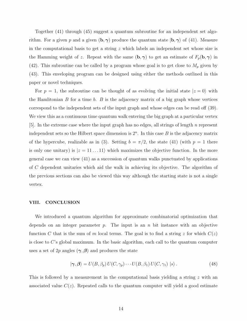
Together (41) through (45) suggest a quantum subroutine for an independent set algo-

rithm. For a given p and a given (b,γ) produce the quantum state |b,γ〉 of (41). Measure

in the computational basis to get a string z which labels an independent set whose size is

the Hamming weight of z. Repeat with the same (b,γ) to get an estimate of Fp(b,γ) in

(42). This subroutine can be called by a program whose goal is to get close to Mp given by

(43). This enveloping program can be designed using either the methods outlined in this

paper or novel techniques.

For p = 1, the subroutine can be thought of as evolving the initial state |z = 0〉 with

the Hamlitonian B for a time b. B is the adjacency matrix of a big graph whose vertices

correspond to the independent sets of the input graph and whose edges can be read off (39).

We view this as a continuous time quantum walk entering the big graph at a particular vertex

[5]. In the extreme case where the input graph has no edges, all strings of length n represent

independent sets so the Hilbert space dimension is 2n. In this case B is the adjacency matrix

of the hypercube, realizable as in (3). Setting b = π/2, the state (41) (with p = 1 there

is only one unitary) is |z = 11 . . . 11〉 which maximizes the objective function. In the more

general case we can view (41) as a succession of quantum walks punctuated by applications

of C dependent unitaries which aid the walk in achieving its objective. The algorithm of

the previous sections can also be viewed this way although the starting state is not a single

vertex.

VIII. CONCLUSION

We introduced a quantum algorithm for approximate combinatorial optimization that

depends on an integer parameter p. The input is an n bit instance with an objective

function C that is the sum of m local terms. The goal is to find a string z for which C(z)

is close to C’s global maximum. In the basic algorithm, each call to the quantum computer

uses a set of 2p angles (γ,β) and produces the state

|γ,β〉 = U(B, βp)U(C, γp) · · ·U(B, β1)U(C, γ1) |s〉 . (48)

This is followed by a measurement in the computational basis yielding a string z with an

associated value C(z). Repeated calls to the quantum computer will yield a good estimate

14

of

Fp(γ,β) = 〈γ,β|C |γ,β〉 . (49)

Running the algorithm requires a strategy for a picking a sequence of sets of angles with the

goal of making Fp as big as possible. We give several possible strategies for finding a good

set of angles.

In section II we focused on fixed p and the case where each bit is in no more than a fixed

number of clauses. In this case there is an efficient classical algorithm that determines the

best set of angles which is then fed to the quantum computer. Here the quantum computer

is run with only the best set of angles. Note that the “efficient” classical algorithm which

evaluates (25) using (24) could require space doubly exponential in p.

An alternative to using a classical preprocessor to find the best angles is to make repeated

calls to the quantum computer with different sets of angles. One strategy, when p does not

grow with n is to put a fine grid on the compact set [0, 2π]p × [0, π]p where the number of

points is only polynomial in n and m. This works because the function Fp does not have

peaks that are so narrow that they are not seen by the grid.

The QAOA can be run on a quantum computer with p growing with n as long as there is a

strategy for choosing sets of angles. Perhaps for some combinatorial optimization problem,

good angles can be discovered in advance. Or the quantum computer can be called to

evaluate Fp(γ,β), the expectation of C in the state |γ,β〉. This call can be used as a

subroutine by a classical algorithm that seeks the maximum of the smooth function Fp(γ,β).

We hope that either p fixed or growing slowly with n will be enough to have this quantum

algorithm be of use in finding solutions to combinatorial search problems beyond what

classical algorithms can achieve.

IX. ACKNOWLEDGEMENTS

This work was supported by the US Army Research Laboratory’s Army Research Office

through grant number W911NF-12-1-0486, and the National Science Foundation through

grant number CCF-121-8176. The authors thank Elizabeth Crosson for discussion and help

in preparing the manuscript. We also thank Cedric Lin and Han-Hsuan Lin for their help.

EF would like to thank the Google Quantum Artificial Intelligence Lab for discussion and

15

support.

[1] Eran Halperin, Dror Livnat, Uri Zwick.

MAX CUT in cubic graphs, 2004.

Journal of Algorithms, Volume 53 Issue 2, Pages 169-185.

[2] Edward Farhi, Jeffrey Goldstone, Sam Gutmann, Michael Sipser.

Quantum computation by adiabatic evolution, 2000.

arXiv:quant-ph/0001106.

[3] Edward Farhi, Jeffrey Goldstone, Sam Gutmann.

Quantum Adiabatic Evolution Algorithms versus Simulated Annealing, 2002.

arXiv:quant-ph/0201031.

[4] Elizabeth Crosson, Edward Farhi, Cedric Yen-Yu Lin, Han-Hsuan Lin, Peter Shor.

Different strategies for optimization with the quantum adiabatic algorithm, 2014.

arXiv:1401.7320 [quant-ph].

[5] Edward Farhi, Sam Gutmann.

Quantum Computation and Decision Trees, 1997.

Phys. Rev. A 58, 915 arXiv:quant-ph/9706062.

16