algorithms for time-aware recommender systems · t time-aware factor models –static factor model...
TRANSCRIPT
t
Algorithms for time-aware recommender systems
A presentation by Sami Diaf and Carlo Morgenstern
t Structure1. Topic and Motivation
2. Paper: Collaborative Filtering with Temporal Dynamics
1. Objective
2. Preliminaries
3. Time-aware factor models
4. Time changing factor model
5. Temporal dynamics at neighbourhood models
6. Conclusion
3. Paper: Multiverse recommendation: n-dimensional tensor factorization for context-aware collaborative filtering
1. Objective
2. Preliminaries
3. General Tensor Factorization
4. Tensor Factorization for Collaborative Filtering
5. Regularization and Optimization
6. Pseudocode
7. Conclusion
4. Comparison of the algorithms
20/12/2016 Algorithms for time-aware recommender systems 2
t Topic and Motivation
Data is changing over time, thus, there is a constant need to
update models in order to reflect its present nature.
Analysis of such data should find the right balance between:
Discounting temporary effects (having a low impact on future behaviour)
Long–term trends reflecting the inherent nature of data
Example : seasonal changes (specific holidays) leading to
shopping patterns
20.12.2016 Algorithms for time-aware recommender systems 3
1
2
3
4
t Topic and Motivation
Item–side effects:
Product perceptions and popularity are in a constant change.
Seasonal patterns influence item’s popularity.
User–side effects: Customers redefine their tastes.
Transient, short–term bias, anchoring
Drifting rating scale
Change of rater within the household
20.12.2016 Algorithms for time-aware recommender systems 4
1
2
3
4
t
Collaborative Filtering with Temporal Dynamics
20.12.2016 Algorithms for time-aware recommender systems 5
1
2
3
4
By Yehuda Koren

t Objective
The primary objective of the paper is to model user
preferences for building a recommender system.
Techniques of addressing time–changing user preferences
will serve to build two recommender techniques:
– Factor modelling
– Item–item neighbourhood
20.12.2016 Algorithms for time-aware recommender systems 6
1
2
3
4
1
2
3
4
5
6
t Objective
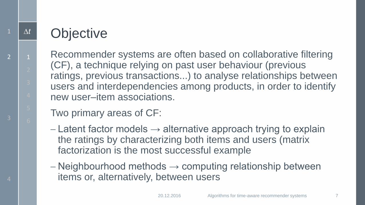
Recommender systems are often based on collaborative filtering (CF), a technique relying on past user behaviour (previous ratings, previous transactions...) to analyse relationships between users and interdependencies among products, in order to identify new user–item associations.
Two primary areas of CF:
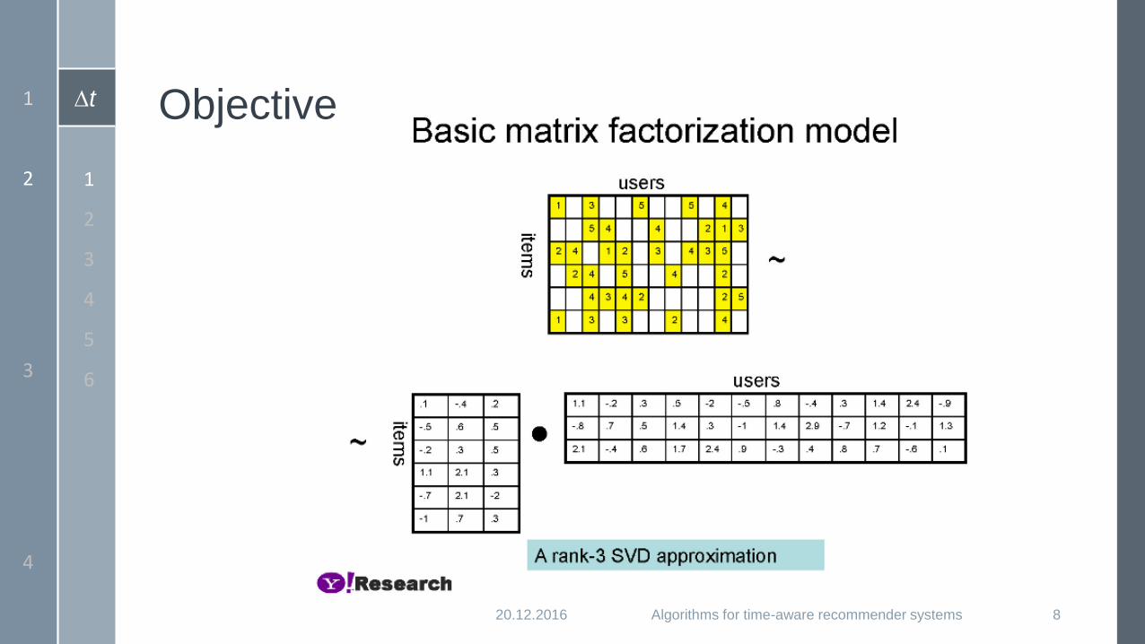
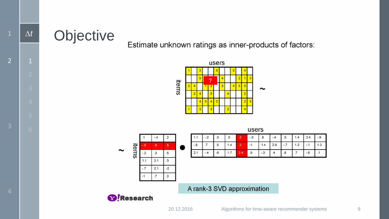
Latent factor models → alternative approach trying to explain the ratings by characterizing both items and users (matrix factorization is the most successful example
Neighbourhood methods → computing relationship between items or, alternatively, between users
20.12.2016 Algorithms for time-aware recommender systems 7
1
2
3
4
1
2
3
4
5
6
t Objective
20.12.2016 Algorithms for time-aware recommender systems 8
1
2
3
4
1
2
3
4
5
6
t Objective
20.12.2016 Algorithms for time-aware recommender systems 9
1
2
3
4
1
2
3
4
5
6
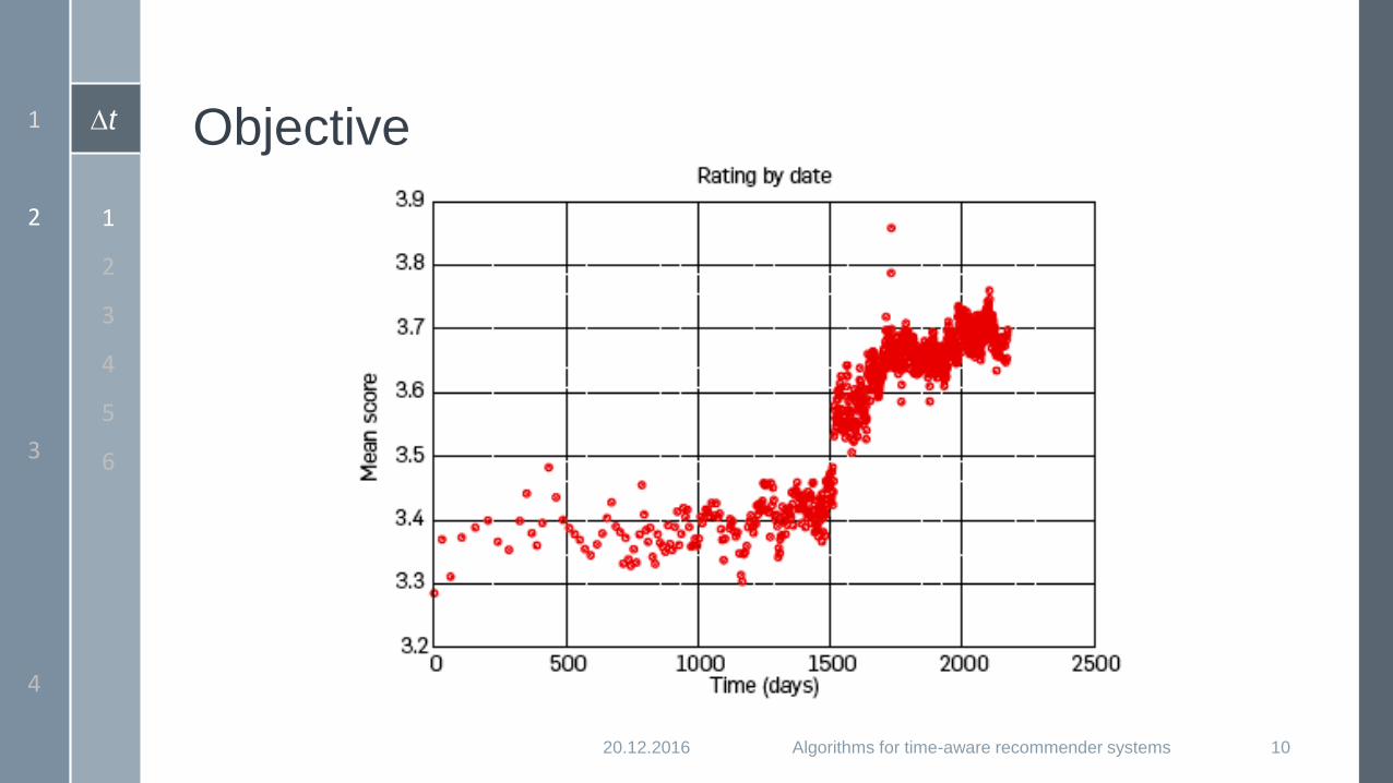
t Objective
20.12.2016 Algorithms for time-aware recommender systems 10
1
2
3
4
1
2
3
4
5
6
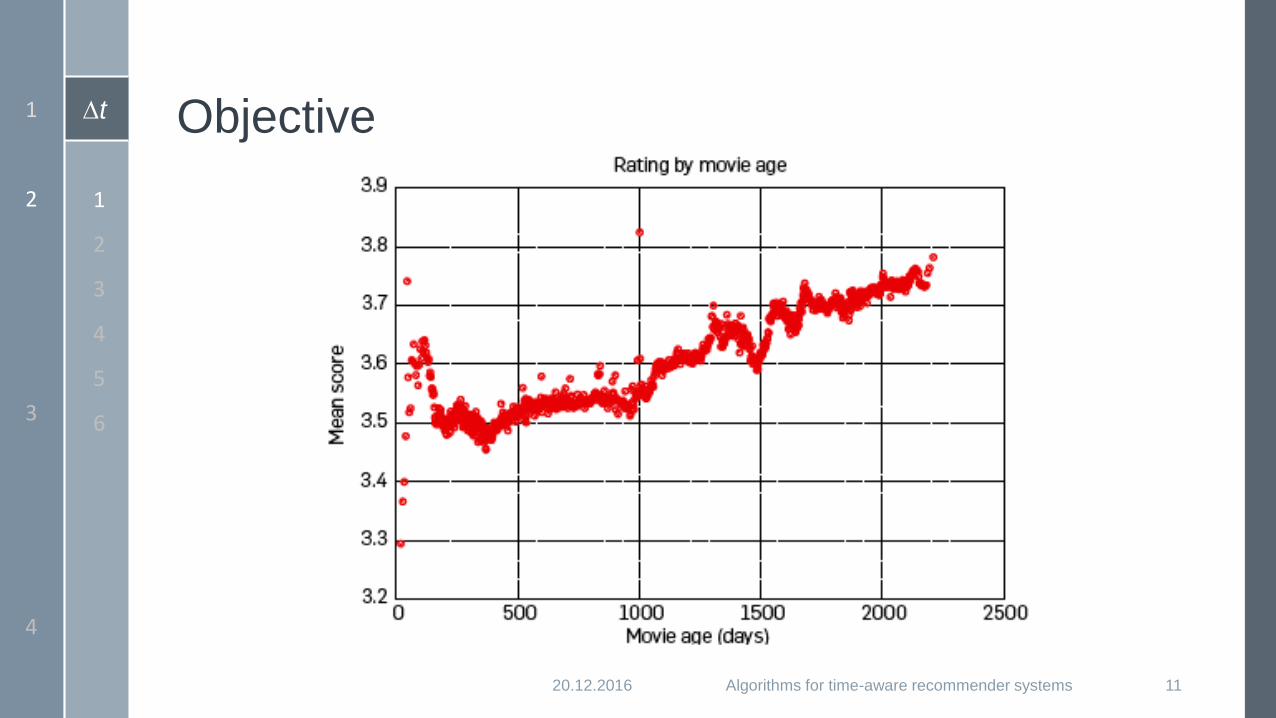
t Objective
20.12.2016 Algorithms for time-aware recommender systems 11
1
2
3
4
1
2
3
4
5
6
t Preliminaries - Notation
20.12.2016 Algorithms for time-aware recommender systems 12
1
2
3
4
1
2
3
4
5
6
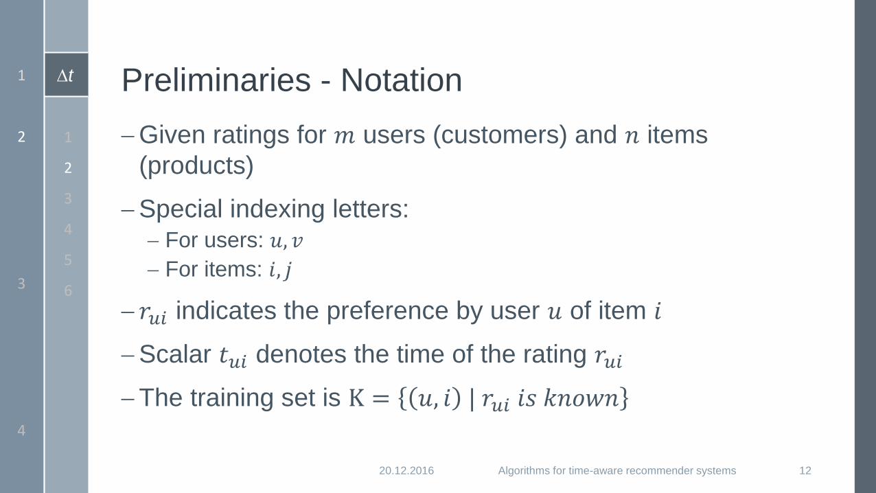
Given ratings for 𝑚 users (customers) and 𝑛 items
(products)
Special indexing letters: For users: 𝑢, 𝑣
For items: 𝑖, 𝑗
𝑟𝑢𝑖 indicates the preference by user 𝑢 of item 𝑖
Scalar 𝑡𝑢𝑖 denotes the time of the rating 𝑟𝑢𝑖
The training set is K = 𝑢, 𝑖 | 𝑟𝑢𝑖 𝑖𝑠 𝑘𝑛𝑜𝑤𝑛
t Preliminaries - Data
20.12.2016 Algorithms for time-aware recommender systems 13
1
2
3
4
1
2
3
4
5
6
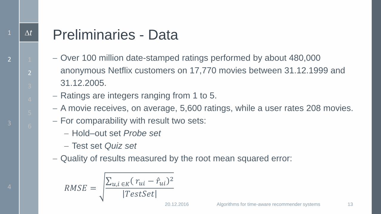
Over 100 million date-stamped ratings performed by about 480,000
anonymous Netflix customers on 17,770 movies between 31.12.1999 and
31.12.2005.
Ratings are integers ranging from 1 to 5.
A movie receives, on average, 5,600 ratings, while a user rates 208 movies.
For comparability with result two sets:
Hold–out set Probe set
Test set Quiz set
Quality of results measured by the root mean squared error:
𝑅𝑀𝑆𝐸 =σ𝑢,𝑖 ∈𝐾 𝑟𝑢𝑖 − Ƹ𝑟𝑢𝑖
2
𝑇𝑒𝑠𝑡𝑆𝑒𝑡

t Time-aware factor models – static factor model
20.12.2016 Algorithms for time-aware recommender systems 14
1
2
3
4
1
2
3
4
5
6
Each user 𝑢 is associated with a vector 𝑝𝑢 ∈ ℜ𝑓
Each item 𝑖 is associated with a vector 𝑞𝑖 ∈ ℜ𝑓
The rating is predicted by:
Ƹ𝑟𝑢𝑖 = 𝑞𝑖𝑇𝑝𝑢 =
𝑘=1
𝑓
𝑞𝑖 𝑘 𝑝𝑢 𝑘
The challenge → computing the mapping of each item and user to factor
vectors 𝑞𝑖 and 𝑝𝑢
Once the mapping accomplished, we can easily compute the ratings a
user will give to any item by using the above equation.
(1)
t Time-aware factor models – static factor model
20.12.2016 Algorithms for time-aware recommender systems 15
1
2
3
4
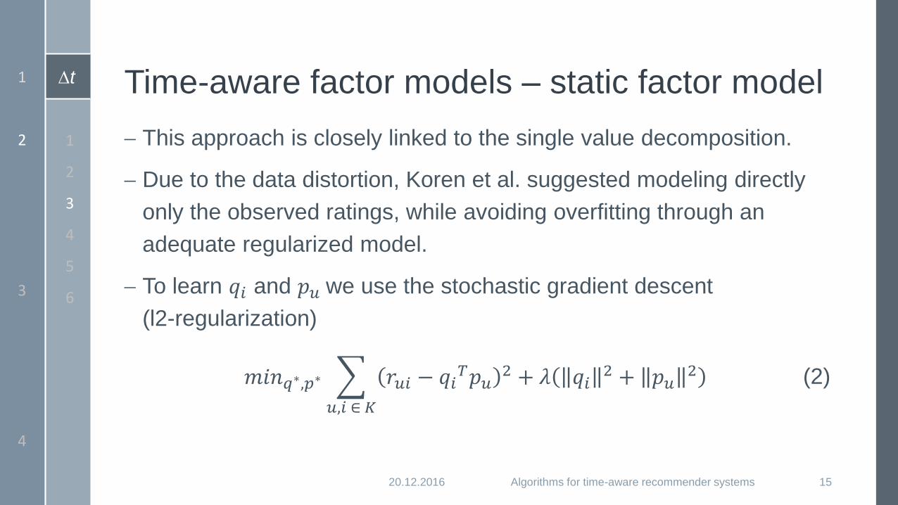
This approach is closely linked to the single value decomposition.
Due to the data distortion, Koren et al. suggested modeling directly
only the observed ratings, while avoiding overfitting through an
adequate regularized model.
To learn 𝑞𝑖 and 𝑝𝑢 we use the stochastic gradient descent
(l2-regularization)
𝑚𝑖𝑛𝑞∗,𝑝∗
𝑢,𝑖 ∈ 𝐾
𝑟𝑢𝑖 − 𝑞𝑖𝑇𝑝𝑢
2 + 𝜆 𝑞𝑖2 + 𝑝𝑢
2 (2)
1
2
3
4
5
6
t Time-aware factor models – static factor model
20.12.2016 Algorithms for time-aware recommender systems 16
1
2
3
4
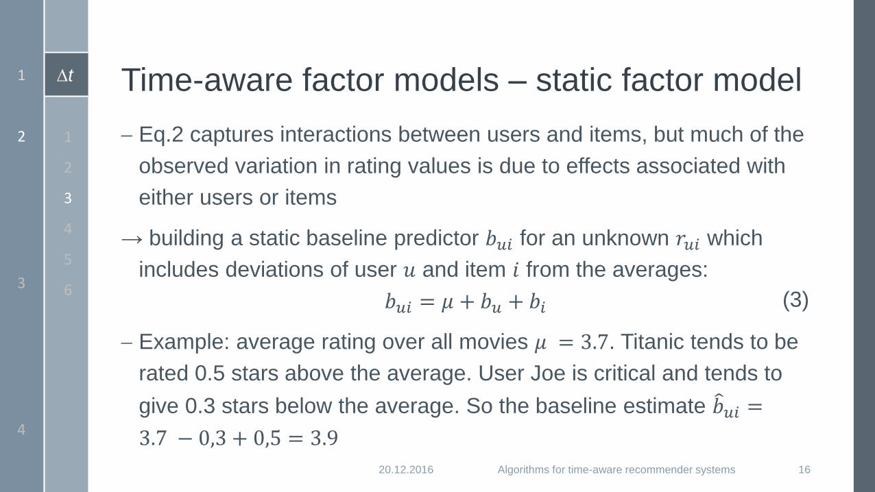
Eq.2 captures interactions between users and items, but much of the
observed variation in rating values is due to effects associated with
either users or items
→ building a static baseline predictor 𝑏𝑢𝑖 for an unknown 𝑟𝑢𝑖 which
includes deviations of user 𝑢 and item 𝑖 from the averages:
𝑏𝑢𝑖 = 𝜇 + 𝑏𝑢 + 𝑏𝑖
Example: average rating over all movies 𝜇 = 3.7. Titanic tends to be
rated 0.5 stars above the average. User Joe is critical and tends to
give 0.3 stars below the average. So the baseline estimate 𝑏𝑢𝑖 =
3.7 − 0,3 + 0,5 = 3.9
(3)
1
2
3
4
5
6

t Time-aware factor models – static factor model
20.12.2016 Algorithms for time-aware recommender systems 17
1
2
3
4
The baseline predictor 𝑏𝑢𝑖 should be integrated in Eq.1
Ƹ𝑟𝑢𝑖 = 𝜇 + 𝑏𝑢 + 𝑏𝑖 + 𝑞𝑖𝑇𝑝𝑢
– 𝜇 the global average
– 𝑏𝑢 the user bias
– 𝑏𝑖 the item bias
– 𝑞𝑖𝑇𝑝𝑢 user-item interaction
Learning is done by minimizing the squared error function
𝑚𝑖𝑛𝑞∗,𝑝∗
𝑢,𝑖 ∈ 𝐾
𝑟𝑢𝑖 − 𝜇 − 𝑏𝑢 − 𝑏𝑖 − 𝑞𝑖𝑇𝑝𝑢
2 + 𝜆 𝑞𝑖2 + 𝑝𝑢
2 + 𝑏𝑢2 + 𝑏𝑖
2
(4)
(5)
1
2
3
4
5
6
t
Time-aware factor models – movie-related temporal effects
20.12.2016 Algorithms for time-aware recommender systems 18
1
2
3
4
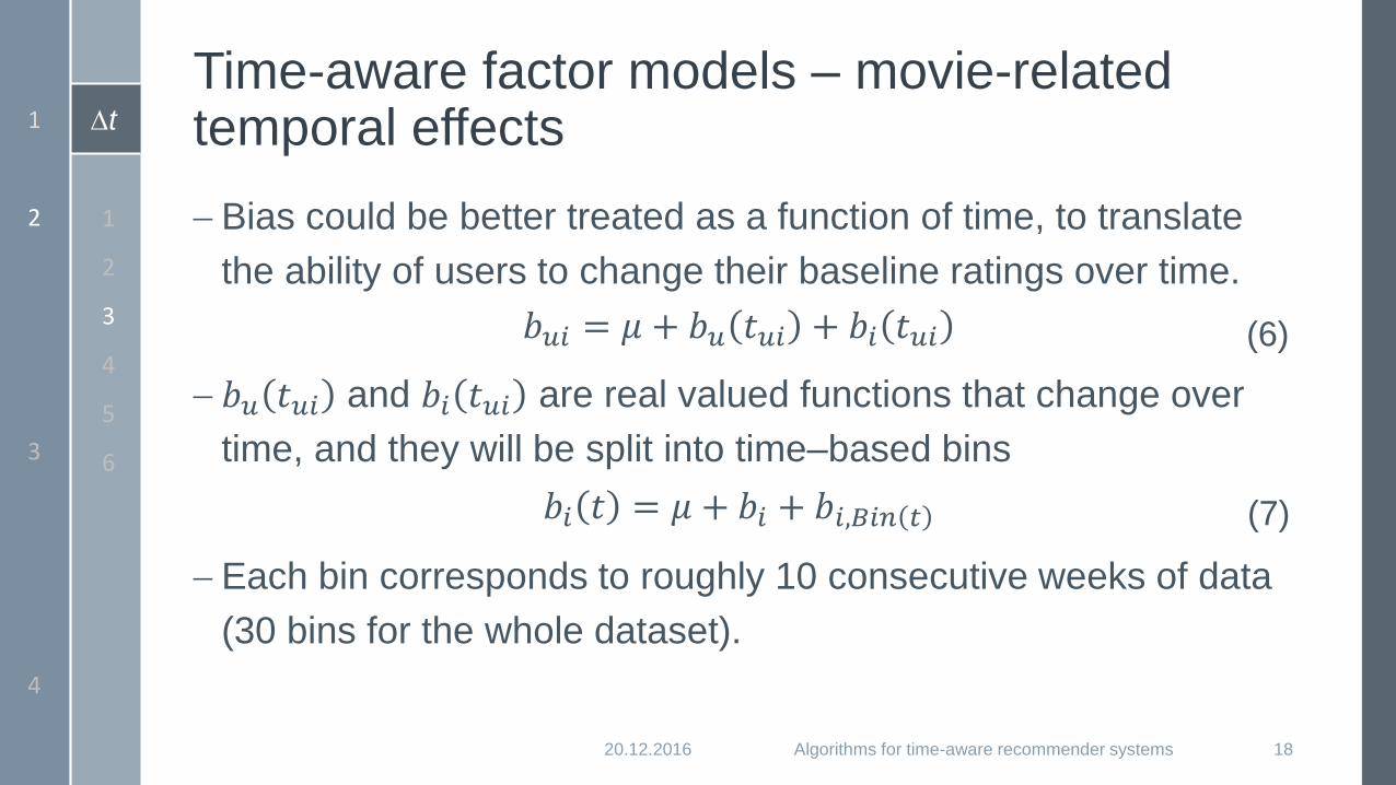
Bias could be better treated as a function of time, to translate
the ability of users to change their baseline ratings over time.
𝑏𝑢𝑖 = 𝜇 + 𝑏𝑢 𝑡𝑢𝑖 + 𝑏𝑖 𝑡𝑢𝑖
𝑏𝑢 𝑡𝑢𝑖 and 𝑏𝑖 𝑡𝑢𝑖 are real valued functions that change over
time, and they will be split into time–based bins
𝑏𝑖 𝑡 = 𝜇 + 𝑏𝑖 + 𝑏𝑖,𝐵𝑖𝑛 𝑡
Each bin corresponds to roughly 10 consecutive weeks of data
(30 bins for the whole dataset).
(6)
(7)
1
2
3
4
5
6
t
Time-aware factor models – linear modelling of user bias
20.12.2016 Algorithms for time-aware recommender systems 19
1
2
3
4
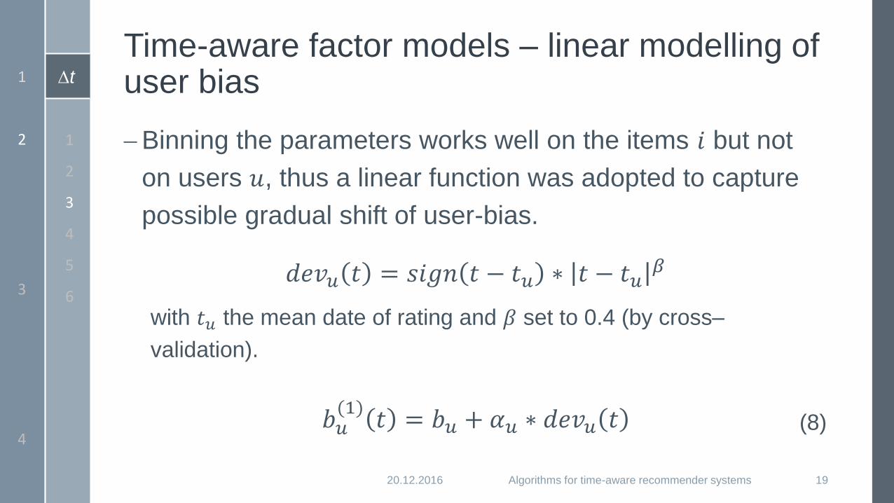
Binning the parameters works well on the items 𝑖 but not
on users 𝑢, thus a linear function was adopted to capture
possible gradual shift of user-bias.
𝑑𝑒𝑣𝑢 𝑡 = 𝑠𝑖𝑔𝑛 𝑡 − 𝑡𝑢 ∗ 𝑡 − 𝑡𝑢𝛽
with 𝑡𝑢 the mean date of rating and 𝛽 set to 0.4 (by cross–
validation).
𝑏𝑢(1)
𝑡 = 𝑏𝑢 + 𝛼𝑢 ∗ 𝑑𝑒𝑣𝑢 𝑡 (8)
1
2
3
4
5
6
t
Time-aware factor models – linear modelling of user bias + single day effect
20.12.2016 Algorithms for time-aware recommender systems 20
1
2
3
4
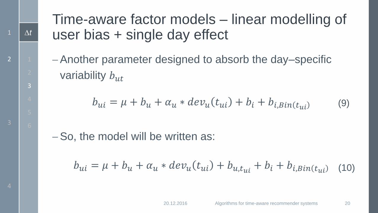
Another parameter designed to absorb the day–specific
variability 𝑏𝑢𝑡
𝑏𝑢𝑖 = 𝜇 + 𝑏𝑢 + 𝛼𝑢 ∗ 𝑑𝑒𝑣𝑢 𝑡𝑢𝑖 + 𝑏𝑖 + 𝑏𝑖,𝐵𝑖𝑛 𝑡𝑢𝑖
So, the model will be written as:
𝑏𝑢𝑖 = 𝜇 + 𝑏𝑢 + 𝛼𝑢 ∗ 𝑑𝑒𝑣𝑢 𝑡𝑢𝑖 + 𝑏𝑢,𝑡𝑢𝑖 + 𝑏𝑖 + 𝑏𝑖,𝐵𝑖𝑛 𝑡𝑢𝑖 (10)
1
2
3
4
5
6
(9)

t Time-aware factor models - Comparison
20.12.2016 Algorithms for time-aware recommender systems 21
1
2
3
4
Model Static model Movie-relatedLinear user
bias
Linear user
bias +
RMSE 0.9799 0.9771 0.9731 0.9605
1
2
3
4
5
6
t
Time-aware factor models – Capturing periodic effect
20.12.2016 Algorithms for time-aware recommender systems 22
1
2
3
4
1
2
3
4
5
6
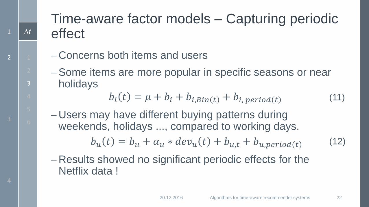
Concerns both items and users
Some items are more popular in specific seasons or near holidays
𝑏𝑖 𝑡 = 𝜇 + 𝑏𝑖 + 𝑏𝑖,𝐵𝑖𝑛 𝑡 + 𝑏𝑖, 𝑝𝑒𝑟𝑖𝑜𝑑 𝑡
Users may have different buying patterns during weekends, holidays ..., compared to working days.
𝑏𝑢 𝑡 = 𝑏𝑢 + 𝛼𝑢 ∗ 𝑑𝑒𝑣𝑢 𝑡 + 𝑏𝑢,𝑡 + 𝑏𝑢,𝑝𝑒𝑟𝑖𝑜𝑑 𝑡
Results showed no significant periodic effects for the Netflix data !
(11)
(12)
t
Time-aware factor models – Changing scale of user rating
20.12.2016 Algorithms for time-aware recommender systems 23
1
2
3
4
1
2
3
4
5
6
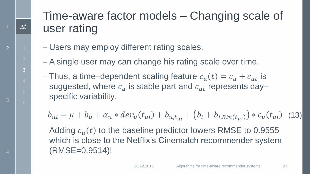
Users may employ different rating scales.
A single user may can change his rating scale over time.
Thus, a time–dependent scaling feature 𝑐𝑢 𝑡 = 𝑐𝑢 + 𝑐𝑢𝑡 is
suggested, where 𝑐𝑢 is stable part and 𝑐𝑢𝑡 represents day–
specific variability.
𝑏𝑢𝑖 = 𝜇 + 𝑏𝑢 + 𝛼𝑢 ∗ 𝑑𝑒𝑣𝑢 𝑡𝑢𝑖 + 𝑏𝑢,𝑡𝑢𝑖 + 𝑏𝑖 + 𝑏𝑖,𝐵𝑖𝑛 𝑡𝑢𝑖 ∗ 𝑐𝑢 𝑡𝑢𝑖
Adding 𝑐𝑢 𝑡 to the baseline predictor lowers RMSE to 0.9555
which is close to the Netflix’s Cinematch recommender system
(RMSE=0.9514)!
(13)
t Time changing factor model
20.12.2016 Algorithms for time-aware recommender systems 24
1
2
3
4
1
2
3
4
5
6
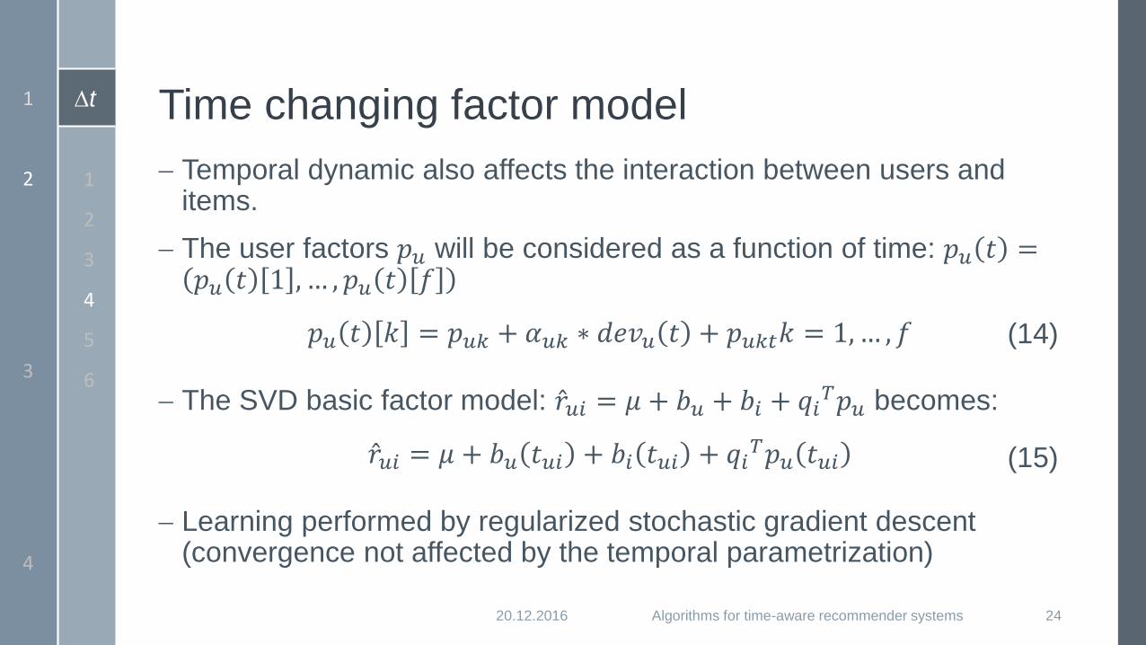
Temporal dynamic also affects the interaction between users and items.
The user factors 𝑝𝑢 will be considered as a function of time: 𝑝𝑢 𝑡 =𝑝𝑢 𝑡 1 , … , 𝑝𝑢 𝑡 𝑓
𝑝𝑢 𝑡 𝑘 = 𝑝𝑢𝑘 + 𝛼𝑢𝑘 ∗ 𝑑𝑒𝑣𝑢 𝑡 + 𝑝𝑢𝑘𝑡𝑘 = 1,… , 𝑓
The SVD basic factor model: Ƹ𝑟𝑢𝑖 = 𝜇 + 𝑏𝑢 + 𝑏𝑖 + 𝑞𝑖𝑇𝑝𝑢 becomes:
Ƹ𝑟𝑢𝑖 = 𝜇 + 𝑏𝑢 𝑡𝑢𝑖 + 𝑏𝑖 𝑡𝑢𝑖 + 𝑞𝑖𝑇𝑝𝑢 𝑡𝑢𝑖
Learning performed by regularized stochastic gradient descent (convergence not affected by the temporal parametrization)
(14)
(15)
t
Time changing factor model – factor models used in practice
20.12.2016 Algorithms for time-aware recommender systems 25
1
2
3
4
1
2
3
4
5
6
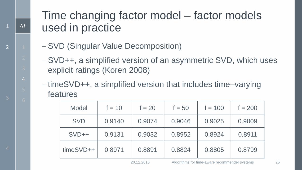
SVD (Singular Value Decomposition)
SVD++, a simplified version of an asymmetric SVD, which uses
explicit ratings (Koren 2008)
timeSVD++, a simplified version that includes time–varying
features
Model f = 10 f = 20 f = 50 f = 100 f = 200
SVD 0.9140 0.9074 0.9046 0.9025 0.9009
SVD++ 0.9131 0.9032 0.8952 0.8924 0.8911
timeSVD++ 0.8971 0.8891 0.8824 0.8805 0.8799
t
Temporal dynamics at neighbourhood models – Static model
20.12.2016 Algorithms for time-aware recommender systems 26
1
2
3
4
1
2
3
4
5
6
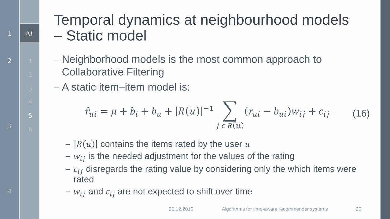
Neighborhood models is the most common approach to
Collaborative Filtering
A static item–item model is:
Ƹ𝑟𝑢𝑖 = 𝜇 + 𝑏𝑖 + 𝑏𝑢 + 𝑅 𝑢 −1
𝑗 𝜖 𝑅 𝑢
𝑟𝑢𝑖 − 𝑏𝑢𝑖 𝑤𝑖𝑗 + 𝑐𝑖𝑗
– 𝑅 𝑢 contains the items rated by the user 𝑢
– 𝑤𝑖𝑗 is the needed adjustment for the values of the rating
– 𝑐𝑖𝑗 disregards the rating value by considering only the which items were rated
– 𝑤𝑖𝑗 and 𝑐𝑖𝑗 are not expected to shift over time
(16)
t
Temporal dynamics at neighbourhood models – Time-varying model
20.12.2016 Algorithms for time-aware recommender systems 27
1
2
3
4
1
2
3
4
5
6
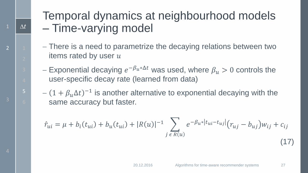
There is a need to parametrize the decaying relations between two
items rated by user 𝑢
Exponential decaying 𝑒−𝛽𝑢∗Δ𝑡 was used, where 𝛽𝑢 > 0 controls the
user-specific decay rate (learned from data)
1 + 𝛽𝑢Δ𝑡−1 is another alternative to exponential decaying with the
same accuracy but faster.
Ƹ𝑟𝑢𝑖 = 𝜇 + 𝑏𝑖 𝑡𝑢𝑖 + 𝑏𝑢 𝑡𝑢𝑖 + 𝑅 𝑢 −1
𝑗 𝜖 𝑅 𝑢
𝑒−𝛽𝑢∗ 𝑡𝑢𝑖−𝑡𝑢𝑗 𝑟𝑢𝑗 − 𝑏𝑢𝑗 𝑤𝑖𝑗 + 𝑐𝑖𝑗
(17)
t
Temporal dynamics at neighbourhood models – Time-varying model
20.12.2016 Algorithms for time-aware recommender systems 28
1
2
3
4
1
2
3
4
5
6
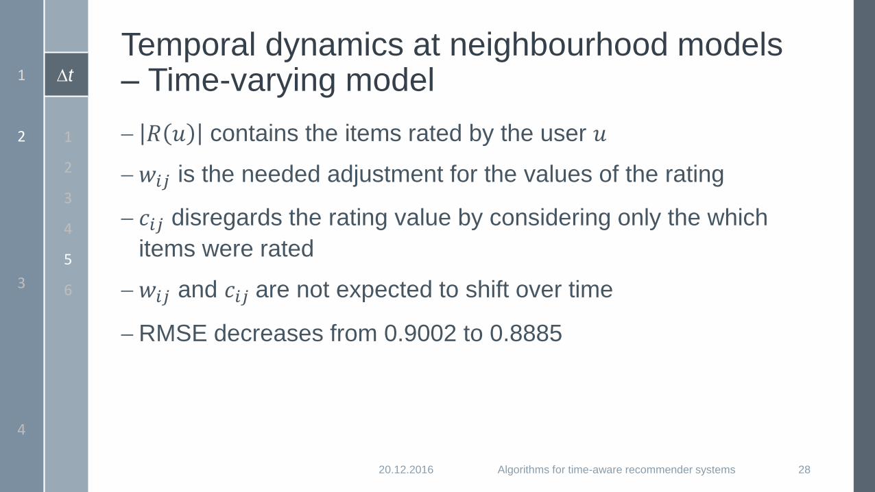
𝑅 𝑢 contains the items rated by the user 𝑢
𝑤𝑖𝑗 is the needed adjustment for the values of the rating
𝑐𝑖𝑗 disregards the rating value by considering only the which
items were rated
𝑤𝑖𝑗 and 𝑐𝑖𝑗 are not expected to shift over time
RMSE decreases from 0.9002 to 0.8885

t
Temporal dynamics at neighbourhood models – Time-varying model
20.12.2016 Algorithms for time-aware recommender systems 29
1
2
3
4
1
2
3
4
5
6
t Conclusion
20.12.2016 Algorithms for time-aware recommender systems 30
1
2
3
4
1
2
3
4
5
6
Modelling temporal effects significantly improves
recommenders accuracy.
Multiple time drifting patterns across users and items.
Sudden single–day effects are significant.
Past temporal fluctuations may help predict future
behaviour.
t
Multiverse Recommendation: N-dimensional Tensor Factorization for Context-aware Collaborative Filtering
20.12.2016 Algorithms for time-aware recommender systems 31
1
2
3
4
By Alexandros Karatzoglou, Xavier Amatriain, Linas Baltrunas and Nuria Oliver
t Objective
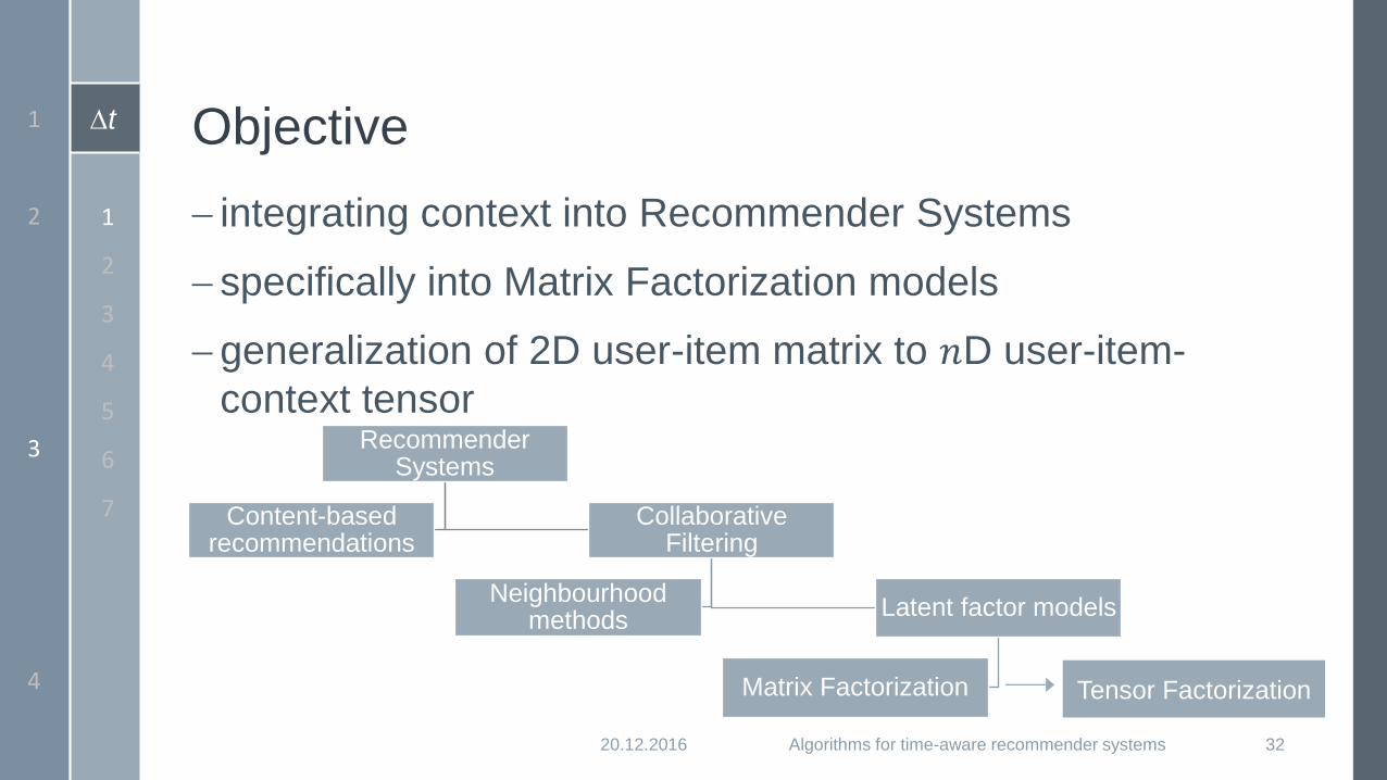
integrating context into Recommender Systems
specifically into Matrix Factorization models
generalization of 2D user-item matrix to 𝑛D user-item-
context tensor
20.12.2016 Algorithms for time-aware recommender systems 32
1
2
3
4
1
2
3
4
5
6
7
Recommender Systems
Content-based recommendations
Collaborative Filtering
Neighbourhoodmethods
Latent factor models
Matrix Factorization Tensor Factorization
t Preliminaries
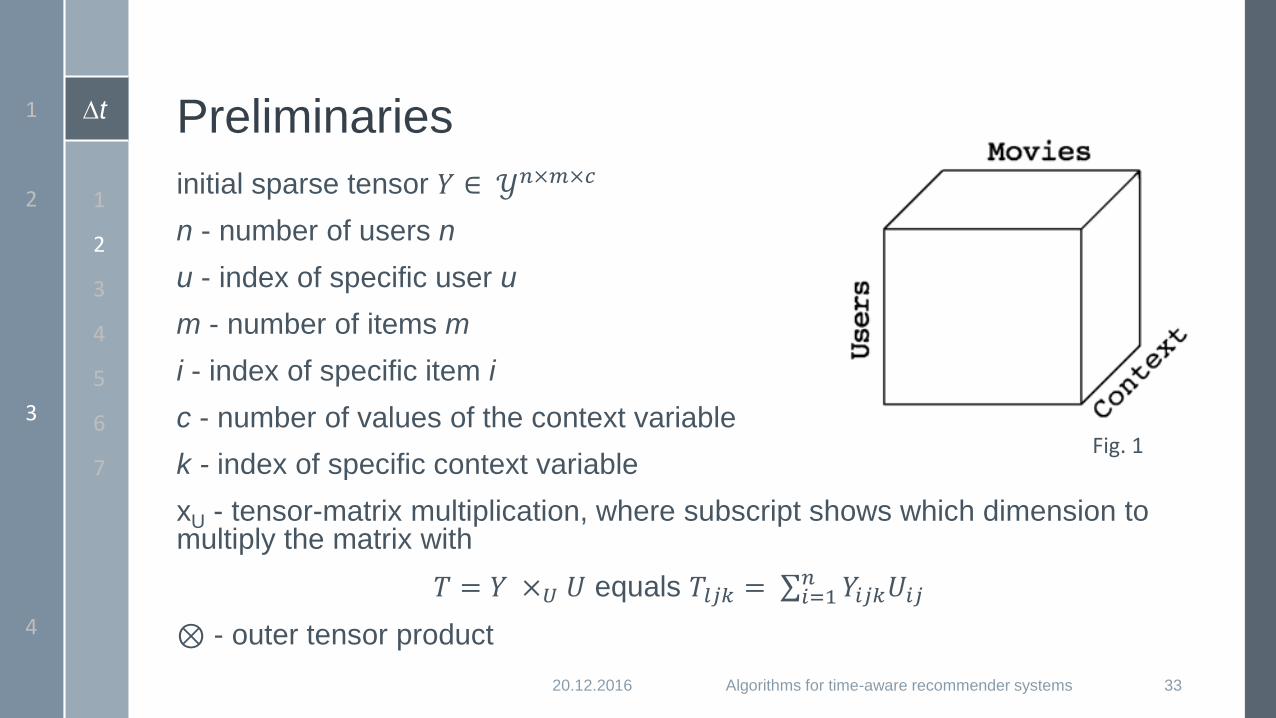
initial sparse tensor 𝑌 ∈ 𝒴𝑛×𝑚×𝑐
n - number of users n
u - index of specific user u
m - number of items m
i - index of specific item i
c - number of values of the context variable
k - index of specific context variable
xU - tensor-matrix multiplication, where subscript shows which dimension to multiply the matrix with
𝑇 = 𝑌 ×𝑈 𝑈 equals 𝑇𝑙𝑗𝑘 = σ𝑖=1𝑛 𝑌𝑖𝑗𝑘𝑈𝑖𝑗
⊗ - outer tensor product
20.12.2016 Algorithms for time-aware recommender systems 33
1
2
3
4
1
2
3
4
5
6
7Fig. 1
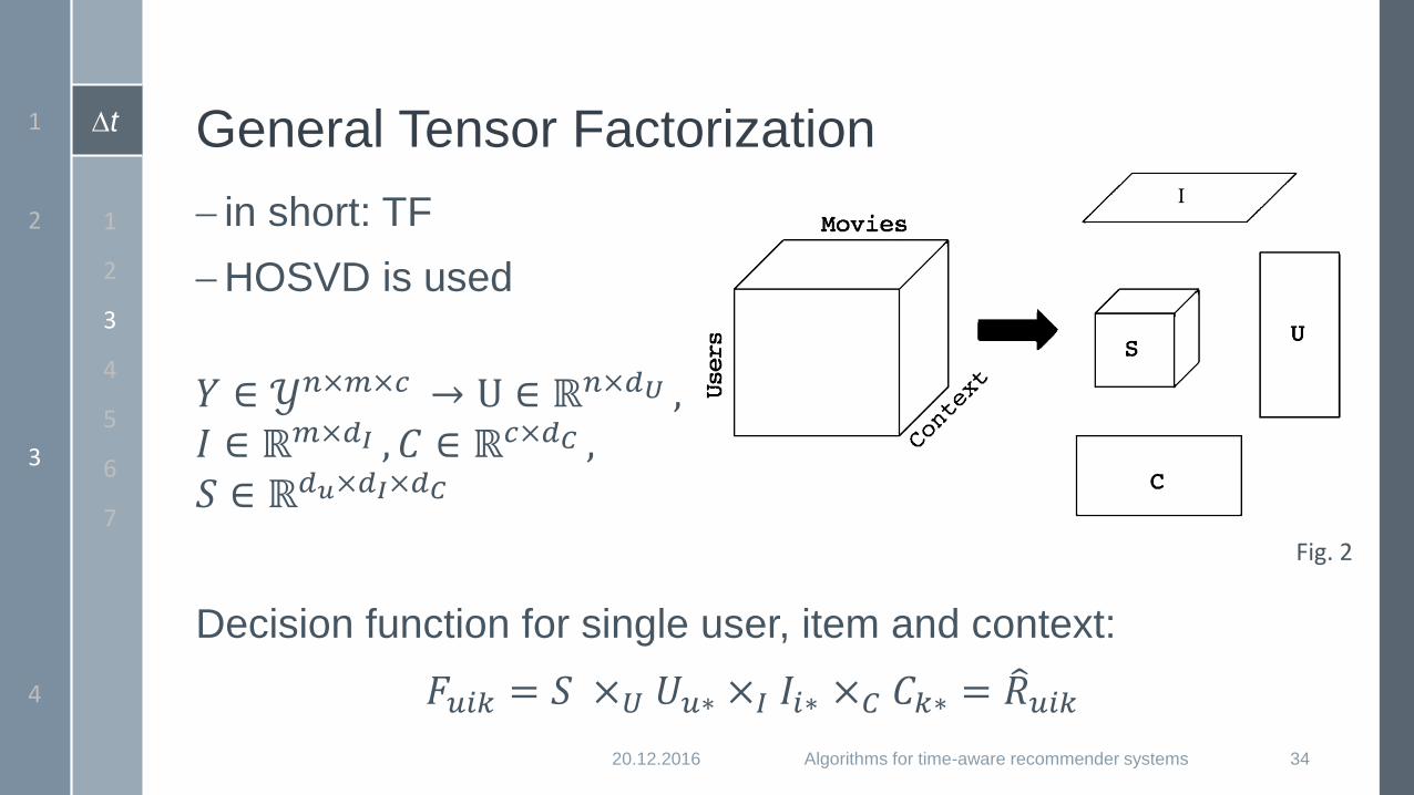
t General Tensor Factorization
in short: TF
HOSVD is used
𝑌 ∈ 𝒴𝑛×𝑚×𝑐 → U ∈ ℝ𝑛×𝑑𝑈 ,𝐼 ∈ ℝ𝑚×𝑑𝐼 , 𝐶 ∈ ℝ𝑐×𝑑𝐶 ,𝑆 ∈ ℝ𝑑𝑢×𝑑𝐼×𝑑𝐶
Decision function for single user, item and context:
𝐹𝑢𝑖𝑘 = 𝑆 ×𝑈 𝑈𝑢∗ ×𝐼 𝐼𝑖∗ ×𝐶 𝐶𝑘∗ = 𝑅𝑢𝑖𝑘
20.12.2016 Algorithms for time-aware recommender systems 34
1
2
3
4
1
2
3
4
5
6
7
Fig. 2
I
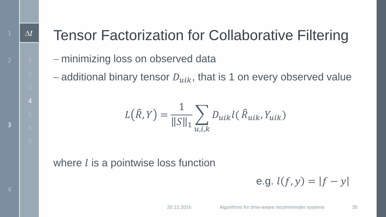
t Tensor Factorization for Collaborative Filtering
minimizing loss on observed data
additional binary tensor 𝐷𝑢𝑖𝑘, that is 1 on every observed value
𝐿 𝑅, 𝑌 =1
𝑆 1
𝑢,𝑖,𝑘
𝐷𝑢𝑖𝑘𝑙( 𝑅𝑢𝑖𝑘 , 𝑌𝑢𝑖𝑘)
where 𝑙 is a pointwise loss function
e.g. 𝑙 𝑓, 𝑦 = 𝑓 − 𝑦
20.12.2016 Algorithms for time-aware recommender systems 35
1
2
3
4
1
2
3
4
5
6
7
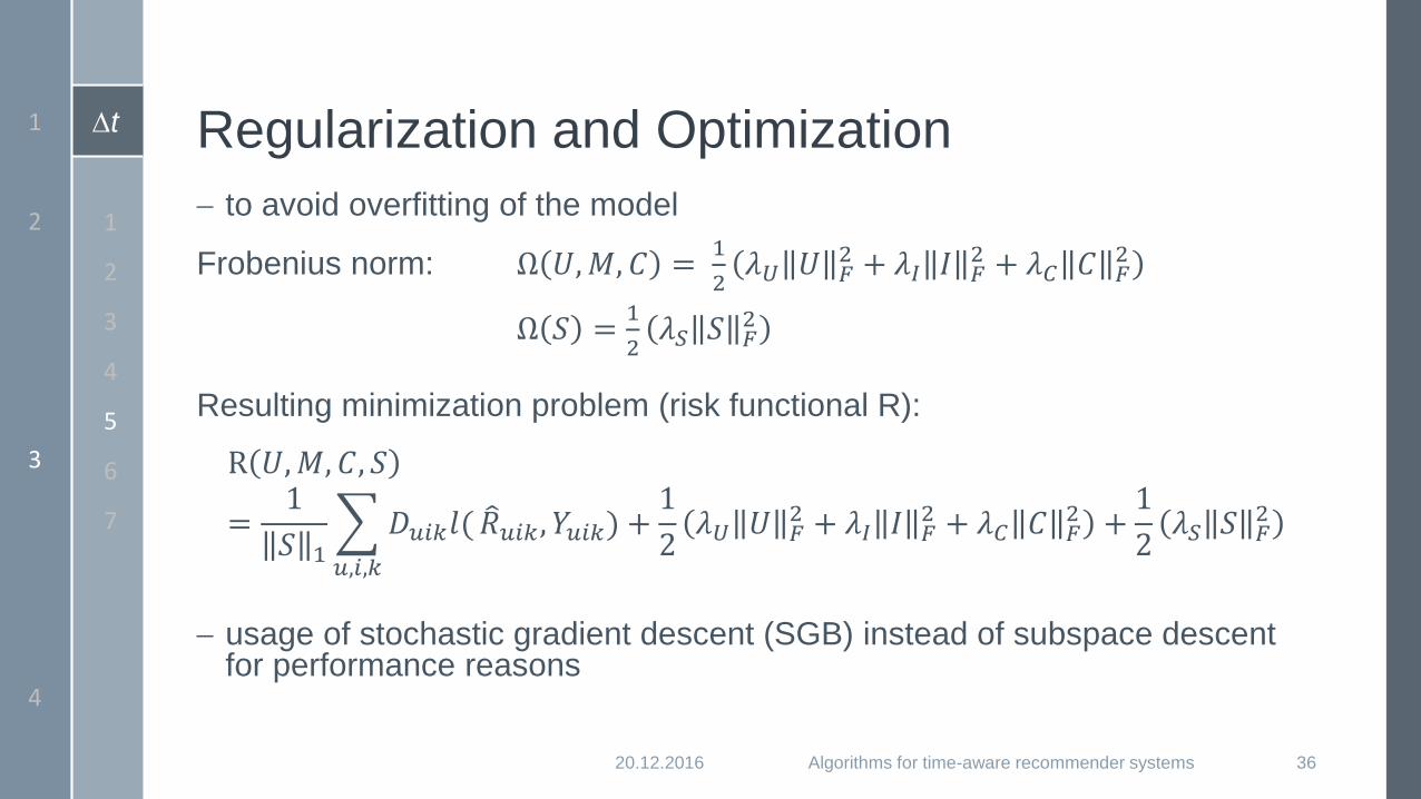
t Regularization and Optimization
to avoid overfitting of the model
Frobenius norm: Ω 𝑈,𝑀, 𝐶 =1
2𝜆𝑈 𝑈 𝐹
2 + 𝜆𝐼 𝐼 𝐹2 + 𝜆𝐶 𝐶 𝐹
2
Ω 𝑆 =1
2𝜆𝑆 𝑆 𝐹
2
Resulting minimization problem (risk functional R):
R 𝑈,𝑀, 𝐶, 𝑆
=1
𝑆 1
𝑢,𝑖,𝑘
𝐷𝑢𝑖𝑘𝑙( 𝑅𝑢𝑖𝑘 , 𝑌𝑢𝑖𝑘) +1
2𝜆𝑈 𝑈 𝐹
2 + 𝜆𝐼 𝐼 𝐹2 + 𝜆𝐶 𝐶 𝐹
2 +1
2𝜆𝑆 𝑆 𝐹
2
usage of stochastic gradient descent (SGB) instead of subspace descent for performance reasons
20.12.2016 Algorithms for time-aware recommender systems 36
1
2
3
4
1
2
3
4
5
6
7
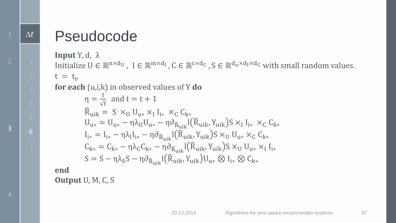
t PseudocodeInput Y, d, λ
Initialize U ∈ ℝn×dU , I ∈ ℝm×dI , C ∈ ℝc×dC , S ∈ ℝdu×dI×dC with small random values.
t = t0for each (u,i,k) in observed values of Y do
η =1
tand t = t + 1
Ruik = S ×U Uu∗ ×I Ii∗ ×C Ck∗Uu∗ = Uu∗ − ηλUUu∗ − η𝜕Ruikl
Ruik, Yuik S ×I Ii∗ ×C Ck∗
Ii∗ = Ii∗ − ηλIIi∗ − η𝜕RuiklRuik, Yuik S ×U Uu∗ ×C Ck∗
Ck∗ = Ck∗ − ηλCCk∗ − η𝜕RuiklRuik, Yuik S ×U Uu∗ ×I Ii∗
S = S − ηλSS − η𝜕RuiklRuik, Yuik Uu∗ ⊗ Ii∗ ⊗Ck∗
endOutput U, M, C, S
20.12.2016 Algorithms for time-aware recommender systems 37
1
2
3
4
1
2
3
4
5
6
7
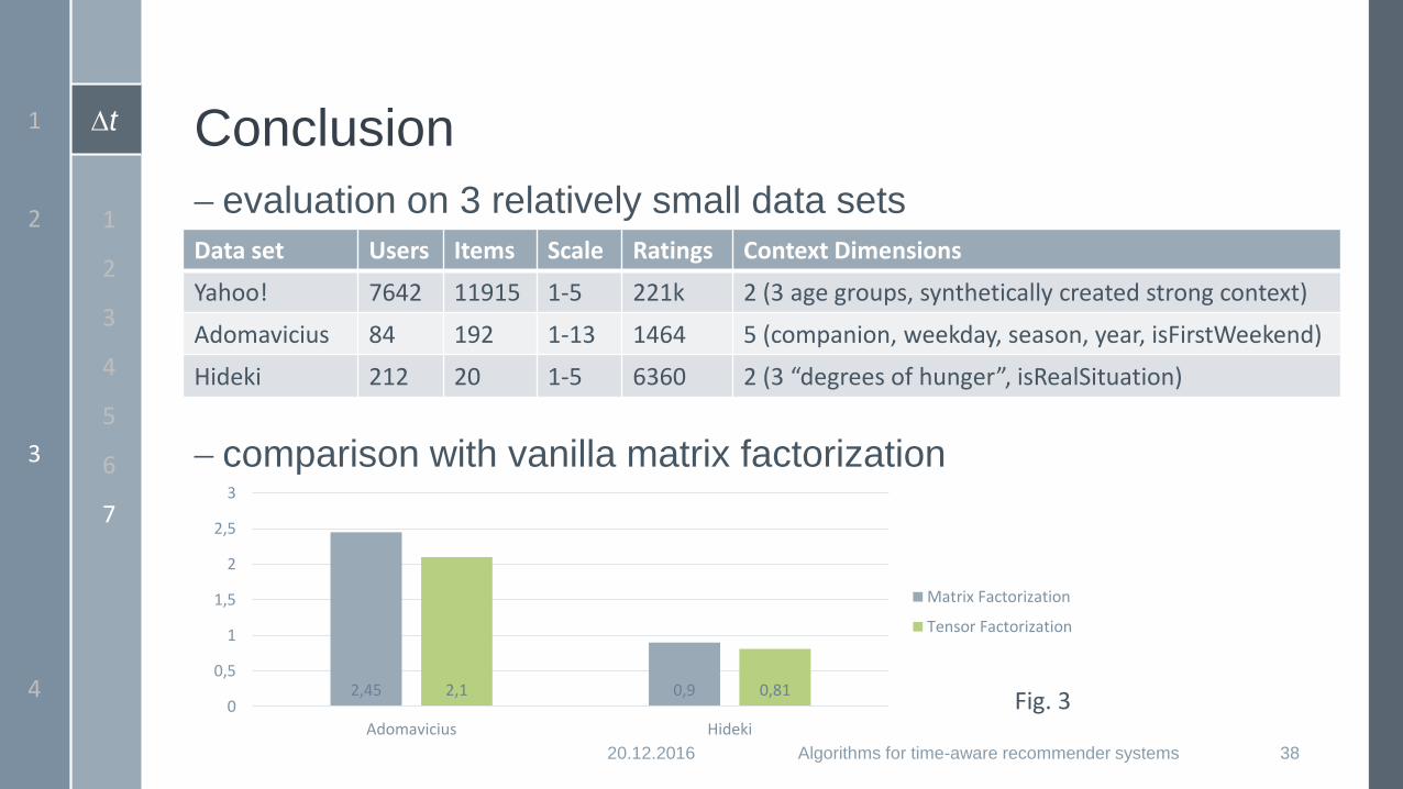
t Conclusion
evaluation on 3 relatively small data sets
comparison with vanilla matrix factorization
20.12.2016 Algorithms for time-aware recommender systems 38
1
2
3
4
1
2
3
4
5
6
7
Data set Users Items Scale Ratings Context Dimensions
Yahoo! 7642 11915 1-5 221k 2 (3 age groups, synthetically created strong context)
Adomavicius 84 192 1-13 1464 5 (companion, weekday, season, year, isFirstWeekend)
Hideki 212 20 1-5 6360 2 (3 “degrees of hunger”, isRealSituation)
2,45 0,92,1 0,810
0,5
1
1,5
2
2,5
3
Adomavicius Hideki
Matrix Factorization
Tensor Factorization
Fig. 3
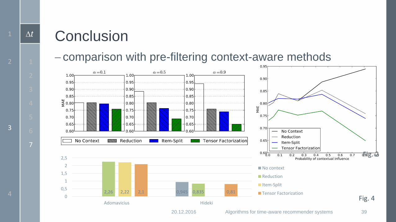
t Conclusion
comparison with pre-filtering context-aware methods
20.12.2016 Algorithms for time-aware recommender systems 39
1
2
3
4
1
2
3
4
5
6
7
0,9452,26 0,8352,22 2,1 0,810
0,5
1
1,5
2
2,5
Adomavicius Hideki
No context
Reduction
Item-Split
Tensor FactorizationFig. 4
Fig. 2
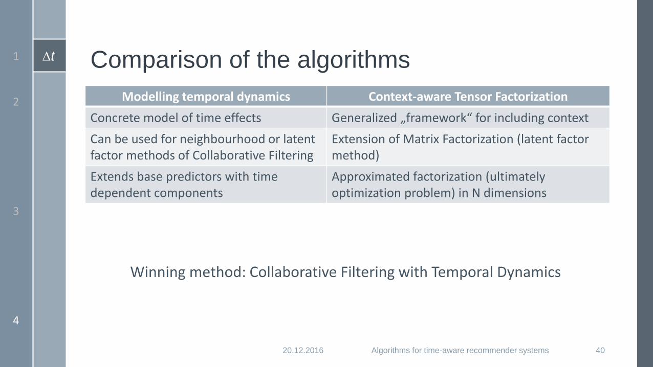
t Comparison of the algorithms
Modelling temporal dynamics Context-aware Tensor Factorization
Concrete model of time effects Generalized „framework“ for including context
Can be used for neighbourhood or latent factor methods of Collaborative Filtering
Extension of Matrix Factorization (latent factor method)
Extends base predictors with time dependent components
Approximated factorization (ultimately optimization problem) in N dimensions
20.12.2016 Algorithms for time-aware recommender systems 40
1
2
3
4
Winning method: Collaborative Filtering with Temporal Dynamics

t
Thank you for your attention!
20.12.2016 Algorithms for time-aware recommender systems 41

t References
Yehuda Koren, Collaborative Filtering with Temporal Dynamics, Communications of the ACM (April 2010), Vol. 53 No. 4
Yehuda Koren, The Bellkor Solution to the Netflix Grand Prize, Netflix prize documentation, 2009
Lei Guo, Matrix Factorization Techniques for Recommender Systems, IRLAB@SDU 2012
Simon Funk, Try this at home, November 2006
Daniel Billsus & Michaels J. Pazzani, Learning Collaborative Information Filters, AAAI 1998
Leskovec, Rajaraman & Ullman, Collaborative Filtering, Stanford University videos
Andrew Ng, Recommender systems: Problem Formulation. Online Open Course
Alexandros Karatzoglou , Xavier Amatriain , Linas Baltrunas , Nuria Oliver, Multiverse recommendation: n-dimensional tensor
factorization for context-aware collaborative filtering, Proceedings of the fourth ACM conference on Recommender systems,
September 26-30, 2010, Barcelona, Spain
G. Adomavicius, R. Sankaranarayanan, S. Sen, and A. Tuzhilin. Incorporating contextual information in recommender systems
using a multidimensional approach. ACM Transactions on Information Systems, 23(1):103–145, 2005
C. Ono, Y. Takishima, Y. Motomura, and H. Asoh. Context-aware preference model based on a study of difference between
real and supposed situation data. In UMAP ’09: Proceedings of the 17th International Conference on User Modeling,
Adaptation, and Personalization, pages 102–113, Berlin, Heidelberg, 2009. Springer-Verlag
20.12.2016 Algorithms for time-aware recommender systems 42