ali badi.pdf
DESCRIPTION
hazemTRANSCRIPT

BEHAVIOUR AND DESIGN OF STEEL COLUMNS SUBJECTED TO VEHICLE IMPACT
A thesis submitted to the University of Manchester for the degree of Doctor of Philosophy in the Faculty of Engineering and Physical Sciences
2012
HAITHAM ALI BADY AL-THAIRY
School of Mechanical, Aerospace and Civil Engineering
2
List of Contents
Page No.
List of Contents ............................................................................................... 2
List of Figures ................................................................................................. 7
List of Tables ................................................................................................... 16
List of Abbreviations and Symbols ................................................................. 18 Chapter One: Introduction 1.1 Statement of the research problem. .......................................................... 28
1.2 Objectives and methodology of the research. ........................................... 29
1.3 Layout of the thesis. .................................................................................. 30 Chapter Two: Literature review 2.1 The research problem ................................................................................ 33
2.2 Current codes of practice ........................................................................... 35
2.3 Previous research studies ........................................................................... 40 2.3.1 Behaviour and failure modes of axially compressed columns under a
transverse impact load ..................................................................... 41 2.3.2 Analytical research studies ..................................................................... 44
2.3.3 Vehicle characteristics ............................................................................ 49
2.3.3.1 Simplifying approaches ............................................................... 51
2.3.3.2 Quantifying vehicle stiffness ....................................................... 52
2.4 Research methodology and originality ...................................................... 55
2.5 Summary .................................................................................................... 56
Chapter Three: Validation of Finite Element Modeling Using ABAQUS/Explicit 3.1 Introduction ................................................................................................ 57
3.2 Dynamic impact analysis using finite element commercial code
ABAQUS/Explicit ........................................................................................... 57 3.2.1 Summary of the explicit dynamics algorithm ......................................... 58
3.2.2 Modelling parameters for structural impact simulation using
ABAQUS/Explicit ................................................................................... 60
3.2.2.1Geometrical modelling ................................................................ 60
3.2.2.2 Material modelling ..................................................................... 61
A. Classical metal plasticity model ........................................................ 62 B. Strain hardening ................................................................................ 62
C. Strain rate dependence ....................................................................... 63
D. Progressive damage and failure for ductile metal ............................. 64
3.2.2.3Modelling of contact .................................................................... 68

3
A. Defining the contact using a contact pair algorithm ......................... 70
B. Defining the contact using the general contact approach .................. 72
3.2.2.4 Stability limit and time increment control................................... 73
3.2.2.5 Damping effects .......................................................................... 74
3.2.2.6 Sequence of axial load application .............................................. 76
3.3 Validation of the numerical model ........................................................... 77 3.3.1 Global plastic buckling failure ................................................................ 78
3.3.1.1Model descriptions ....................................................................... 79
3.3.1.2 Simulation results ........................................................................ 81
3.3.1.3 Damping effect ............................................................................ 82
3.3.2 Tensile tearing failure ............................................................................. 83
3.3.2.1 Model descriptions ...................................................................... 84
3.3.2.2 Modelling of tensile failure ......................................................... 84
3.3.2.3 Simulation results ........................................................................ 85
3.3.3 Shear failure ............................................................................................ 87
3.3.3.1 Model descriptions ..................................................................... 87
3.3.3.2 Modelling of shear failure ........................................................... 88
3.3.3.3 Simulation results ........................................................................ 89
3.4 Summary ................................................................................................... 92 Chapter Four: A Parametric Study of the Behaviour and Failure Modes of Axially Loaded Steel Columns Subjected to a Rigid Mass Impact 4.1 Introduction ................................................................................................ 94
4.2 Parametric study ........................................................................................ 94 4.2.1 Steel columns .......................................................................................... 95
4.2.1.1 Modelling properties ................................................................... 96
4.2.1.2 Mesh size sensitivity ................................................................... 97
4.2.2 The impacting mass ................................................................................ 101
4.2.3 Modelling of contact ............................................................................... 102
4.2.4 Analysis of simulation results ................................................................. 103
4.2.4.1 Failure modes .............................................................................. 103
4.2.4.2 Impact energy .............................................................................. 109
4.2.4.3 Critical impact velocity ............................................................... 113
4.2.4.4 Plastic hinge location .................................................................. 115
4.2.4.5 Effect of impact direction ............................................................ 118
4.2.4.6. Damping effects ......................................................................... 119
4.2.4.7 Effects of strain hardening and strain rate ................................... 120
4.3 Summary .................................................................................................... 122

4
Chapter Five: A simplified FE Vehicle Model for Assessing the Vulnerability of Axially Compressed Steel Columns Against Vehicle Frontal Impact 5.1Introduction ................................................................................................. 124
5.2 Vehicle characteristics .............................................................................. 125
5.3 Simplified vehicle model ........................................................................... 126 5.3.1 Validation ................................................................................................ 127
5.3.1.1 Vehicle impact on a rigid barrier................................................. 127
5.3.1.2 Validation of the spring-mass system against the numerical
simulation of a vehicle impact on a column using a full-scale
numerical vehicle model ............................................................. 131
A. Full scale numerical vehicle model ........................................ 131
B. Validation for vehicle impact on steel columns ..................... 132
5.3.2 Sensitivity of column behaviour to stiffness parameters K1 and K2 ....... 139
5.3.3 Determining an appropriate simplified vehicle model ........................... 141
5.3.4 Effect of increasing vehicle weight ........................................................ 146
5.4 Determination of the equivalent vehicle linear stiffness ........................... 149 5.4.1 Derivation of the vehicle stiffness equation ........................................... 149
5.4.2 Validation of the suggested stiffness equation ....................................... 152
5.5 Summary ................................................................................................... 153 Chapter Six: The Derivations of a Simplified Analytical Method for Predicting the Critical Velocity of Transverse Rigid Body Impact and Vehicle Impact on Steel Columns 6.1 Introduction. .............................................................................................. 155
6.2 Derivations of the simplified analytical method ........................................ 156 6.2.1. Developing the energy balance equation ............................................... 156
6.2.2 Energy absorbed by the column’s deformation (IEcol) ........................... 157
6.2.2.1 Derivations of the maximum elastic and critical rotations ( iElasticθ and
iCriticalθ ) ........................................................................................ 159
A. Selecting the elastic deformation shape .................................... 160
B. Determination of the intermediate plastic hinge location ......... 160
6.2.2.2 Derivations of the internal energy equations for columns under
moderate to high axial loads (P≥25%PDesign) ............................. 162
A. Maximum elastic rotationiElasticθ ............................................ 162
B. Critical rotation iCriticalθ . .......................................................... 163
6.2.2.3 Derivations for the internal energy equation for columns under low
axial load levels (P< 25%PDesign) ................................................. 167
6.2.2.4 Reduced plastic moment capacity ............................................... 169
6.2.3 The energy absorbed by the vehicle (IEv) ............................................... 171

5
A. EN 1993-1-1 (Eurocode 3) ....................................................... 172
B. New proposal ............................................................................ 173
6.2.4 Derivations of the external work equation .............................................. 176
6.2.5 General energy balance equation ............................................................ 177
6.2.6 Accounting for the strain hardening effects ............................................ 178
6.3 Summary .................................................................................................... 179 Chapter Seven: Validation of the Simplified Analytical Method 7.1 Introduction ................................................................................................ 181
7.2 Validation of the analytical method against rigid body impact ................ 182 7.2.1 Maximum column displacements ........................................................... 182
7.2.2 Critical impact velocity-axial load interaction curves ............................ 185
7.2.3 Energy quantities .................................................................................... 188
7.3 Validation of the analytical method against vehicle impact ...................... 193 7.3.1 Critical impact velocity- axial load interaction curves ........................... 195
7.3.2 Energy quantities .................................................................................... 199
7.3.3 Validation of the simplified analytical method against different values of K1
and Cmax ................................................................................................... 201
7.3.4 Using alternative values for the maximum static transverse resistance of
steel columns ........................................................................................... 203
7.4 The strain hardening effect ........................................................................ 206
7.5 Summary .................................................................................................... 207 Chapter Eight: Assessment of the Current Eurocode1 Design Method for Steel Columns under Vehicle Impact 8.1 Introduction ................................................................................................ 209
8.2 The equivalent static force approach ......................................................... 209
8.3 The Dynamic impulse approach ...................................................................... 212
A. Using vehicle stiffness ............................................................................... 213
B. Using column stiffness ............................................................................... 213
8.3.1 A proposed modification ............................................................................ 218
8.4 Summary .................................................................................................... 221 Chapter Nine: Conclusions and Recommendations for Future Research Studies 9.1 Introduction ................................................................................................ 222
9.2 Conclusions of this research .................................................................... 222 9.2.1 Numerical modelling of steel column behaviour under transverse impact
.............................................................................................................. 222
9.2.2 Behaviour and failure modes of steel columns under transverse impact 223
9.2.3 Simplified vehicle model ....................................................................... 224

6
9.2.4 Development of an analytical method for column behaviour under
transverse impact. .................................................................................... 224
9.2.5 Assessment of current design methods in Eurocode 1 ........................... 225
9.3 Recommendations for future research works ............................................ 225
References ........................................................................................................ 228
Appendix A: Publications ................................................................................ 234 Total word count: 42712

7
List of Figures
Figure Contents Page No.
Figure 1.1: Collision of a vehicle with a reinforced concrete support (left); Impact test
(right). Pictures from (Ghose, 2009) ............................................................................... 29
Figure 2.1: Collapse of a bridge after being struck by tractor-trailer (courtesy of NDOR)
(El-Tawil et al., 2005) ..................................................................................................... 33
Figure 2.2: An example of a severe impact involving a 16 ton crane (Courtesy of the
Manchester Evening News)(Ellis, 2003) ........................................................................ 34
Figure 2.3: Deformed lighting pole and vehicle after impact at 100 km/h. (Helsinki
University of Technology) (Klyavin et al., 2008) ........................................................... 34
Figure 2.4: Single degree of freedom SDOF model idealization for the derivation of Eq.
2.2 .................................................................................................................................... 37
Figure 2.5: Idealised impact pulse model (Eurocode1, 2006) ........................................ 38
Figure 2.6: Tensile tearing failure and transverse shear failure of clamped steel beams
under the impact of drop mass (Liu and Jones, 1987) (a): Transverse shear failure at the
impact point, (b)-(d): Tensile tearing failure at the impact ............................................. 42
Figure 2.7: View of the deformed specimens after impact (Zeinoddini et al., 2002) ..... 43
Figure 2.8: Buckling failure of impacted aluminium columns for different impact
velocities (Adachi et al., 2004) ....................................................................................... 43
Figure 2.9: Theoretical model of Bambach et al. (2008) ................................................ 46
Figure 2.10: Idealized system used by Shope (2006) with elastic–perfectly plastic
material behaviour ........................................................................................................... 47
Figure 2.11: Simplified force-deformation behaviour of a concrete column, with and
without strain rate effects (Tsang and Lam, 2008) ......................................................... 48
Figure 2.12: (A) A frontal collision test of a Honda Accord at a speed of 48.3 km/h;(B)
Force-time histories of full scale crash tests for different types of vehicle (from
(Thilakarathna et al., 2010). ............................................................................................ 50
Figure 2.13: Spring-mass system used by Emori (Emori, 1968). ................................... 51
Figure 2.14: Vehicle stiffness characteristics defined by Milner et al. (B. Milner et al.,
2001) ............................................................................................................................... 52
Figure 2.15: An example of a vehicle impact force-crush distance relationship ............ 53
Figure 3.1: The computational algorithm used in ABAQUS/Explicit. (Reproduced from
(SIMULIA, 2010d) )) ...................................................................................................... 59
Figure 3.2: Linear brick, shell and spring elements used in the present numerical
simulation using ABAQUS/Explicit (SIMULIA, 2010b). .............................................. 61
Figure 3.3: Meshing technique used over each thickness of a steel beam using linear
elements with reduced integration. ................................................................................. 61
Figure 3.4: Typical true plastic stress-true plastic strain relationship of steel, including
strain hardening and strain rate effects............................................................................ 63
8
Figure 3.5: Typical uniaxial stress-strain response of the steel with progressive damage
evolution up to failure. .................................................................................................... 65
Figure 3.6: Simulating impact force as a time dependant function force (SIMULIA,
2010d) ............................................................................................................................. 69
Figure 3.7: A contact pairs as master and slave surfaces(SIMULIA, 2010d)................. 70
Figure 3.8: Master surface penetrating into the slave surface of a pure master-slave
contact pair due to improper meshing (SIMULIA, 2010d)............................................. 70
Figure 3.9 Contact pressure-clearance relationship for hard contact (SIMULIA, 2010d)
......................................................................................................................................... 72
Figure 3.10: Smooth step amplitude curve used to define a quasi-static load (SIMULIA,
2010e) .............................................................................................................................. 76
Figure 3.11: Energy histories for a quasi-static structural system (SIMULIA, 2010e) .. 77
Figure 3.12: Experimental set up of Zeinoddini et al. (2002) (top) and the numerical
model (bottom). ............................................................................................................... 79
Figure 3.13: Smooth amplitude functions used to apply the quasi-static load................ 81
Figure 3.14: Energy histories during the quasi-static load application, (P/Py) =0.5. ..... 81
Figure 3.15: Axial displacement – the time history of the impacted steel tube for
different axial load levels. ............................................................................................... 82
Figure 3.16: (A) Comparison of the contact force; (B) Comparison of the deformation
shape for (P/Py)=0.6; for the tests of Zeinoddini et al (2002, Zeinoddini et al., 2008b) 82
Figure 3.17: Effects of damping on the contact force history of the steel tube with
(P/Py)=0.5 ....................................................................................................................... 83
Figure 3.18: Experimental specimen of 50SHS (Bambach et al., 2008) (top) and the
numerical model (bottom). .............................................................................................. 84
Figure 3.19: Deformation shape and tensile fracture at the supports at 20 ms after
impact. Top: experimental result (Bambach et al., 2008). Bottom: numerical simulation
......................................................................................................................................... 85
Figure 3.20: Ductile damage initiation profile history along the top surface of the beam
......................................................................................................................................... 86
Figure 3.21: Ductile damage initiation at the support and at the point of impact ........... 86
Figure 3.22: Numerical model and mesh size of the steel beam with a close-up view of
the mesh at the impact point. .......................................................................................... 87
Figure 3.23: True stress-true strain curve of steel plastic (Yu and Jones, 1991) ............ 88
Figure 3.24: Comparison of the displacement at the impact point of the steel beam SB07
between the experimental results (Yu and Jones, 1991) and the present numerical
simulation ........................................................................................................................ 89
Figure 3.25: Comparison of the deformation shape of the steel specimen SB08 after
shear failure between the experimental test (Yu and Jones, 1991) (top) and the
numerical simulation (bottom). ....................................................................................... 90
Figure 3.26: Comparison of axial strain of steel specimen SB08 on the lower surface
underneath the striker between the experimental results of Yu and Jones (1991) and the
present numerical simulation results ............................................................................... 91

9
Figure 3.27: Shear damage initiation profile at the top and bottom surfaces of the beam
of the steel specimen SB08 along its length ................................................................... 91
Figure 3.28: Stress-strain behaviour of a failed element at the impact zone showing
damage initiation and propagation of the element. ......................................................... 92
Figure 4.1: Meshing technique used for the steel column: A) Longitudinal direction; B)
Cross sectional direction for two steel column sections. ................................................ 96
Figure 4.2: Assumed true stress-strain curve used to simulate S355 material behaviour
in the parametric study. ................................................................................................... 97
Figure 4.3: Sensitivity of the column behaviour to the mesh size of (A) the flange; and
(B) the web, for a simply supported column section UC 305×305×118, P=50%PDesign,
Impacting mass=6 tonnes, V=40 km/h. .......................................................................... 99
Figure 4.4: Sensitivity of the column axial displacement history, V=40 km/h (A) and the
shear damage history at the impact point; V=60 km/h (B) for different mesh sizes,
column section UC 356×406×340, P=50%PDesign, Impacting mass=6 tonnes. ........... 100
Figure 4.5: Sensitivity of the column lateral displacement history at the impact point for
different mesh sizes, column section UC 305×305×118, P=50%PDesign, Impacting
mass=6 tonnes, V=40 km/h. .......................................................................................... 101
Figure 4.6: A close-up view of the element size of the steel column model adopted in
the parametric study ...................................................................................................... 101
Figure 4.7: Shape and dimensions of the impactor used in the parametric study ......... 102
Figure 4.8: Defining the master and slave surfaces in the numerical model ................ 103
Figure 4.9: Local flange distortion at the impact zone for the section UC305×305×118.
....................................................................................................................................... 106
Figure 4.10: Deformed shape history of the columns. (A): a simply supported section
UC 305×305×118, Impact location= 1.0 m, P/P Design =0.5, Impact mass =1 tonnes,
Impact velocity =80 km/h; (B): a simply supported section UC 305×305×118, Impact
location= 1.5 m, P/P Design =0.7, Impact mass =3 tonnes, Impact velocity =20 km/h; (C)
a propped cantilever section UC 305×305×118, Impact location= 1.5 m, P/P Design =0.7,
Impact mass =6 tonnes, Impact velocity =40 km/h ...................................................... 107
Figure 4.11: The axial displacement history for the columns in Fig. 4.10 ................... 108
Figure 4.12: The shear damage initiation criterion profile along the column length for a
simply supported column section UC 356×406×340, impact velocity = 80km/h ....... 108
Figure 4.13: The shear damage initiation criterion profile along the column length for a
simply supported column section UC305×305×118, impact velocity = 80km/h ........ 109
Figure 4.14: The shear damage initiation criterion profile along the column length for
propped cantilever columns and impact velocity = 80km/h; A) section
UC356×406×340; B) section UC305×305×118 ........................................................ 109
Figure 4.15: Behaviour of the simply supported column (section UC 305×305×118,
L=4m, impact location = 1m) under the same impact energy but with different
combinations of impactor mass and velocity. ............................................................... 110
10
Figure 4.16: Behaviour of the propped cantilever column (section UC 305×305×118,
L=4m, impact location = 1.5 m) under the same impact energy but with different
combinations of impactor mass and velocity ................................................................ 111
Figure 4.17: The kinetic energy history of the axially loaded simply supported steel
column (section UC 305×305×118, L=4 m, impact location =1m, P/PDesign=50%,
Impact energy = 117KJ). ............................................................................................... 112
Figure 4.18: Comparison of the total kinetic energy history of the columns without
failure, at the critical condition, with clear failures ...................................................... 113
Figure 4.19: Column mid-height deformation history under different impact speeds,
steel column height L=4 m, Impact mass= 1 tonnes, P/PDesign=50%, impact position
=1m, for a simply support column ................................................................................ 113
Figure 4.20: Energy histories corresponding to impact velocities of (A) 55km/h and (B)
50km/h. ......................................................................................................................... 114
Figure 4.21: Axial force - critical impact velocity interaction curves of the steel columns
used in the parametric study: (A) section UC 356×406×340, L=8 m, impact
mass=6tonnes, impact location =2m); (B) section UC 305×305×118, L=4 m, impact
mass=3tonnes, impact location =1.5m) ......................................................................... 115
Figure 4.22: Effects of axial load level on the intermediate plastic hinge location (A): on
simply supported columns; (B): Propped cantilever columns. Impact mass =3 tonnes.
....................................................................................................................................... 116
Figure 4.23: Collapse shapes showing the intermediate plastic hinge location for
different axial load ratios of simply supported columns (a) L= 8 m, impact location =2
m, Mass =6 tonnes; (b) L= 8 m, impact location =1 m, Mass =3 Ton; (c) L= 4 m, impact
location =1.5 m, Mass =6 tonnes; (d) L= 4 m, impact location=1 m, Mass = 3 tonnes 117
Figure 4.24: Collapse shapes showing the intermediate plastic hinge location for
different axial load ratios of propped cantilever columns (a) L= 8 m, impact location =2
m, Mass = 6 tonnes; (b) L= 4 m, impact location =1.5 m, Mass =3 tonnes. ................. 117
Figure 4.25: 30, 45 and 90 degrees of impact ............................................................... 118
Figure 4.26: Effect of impact direction on the critical impact velocity of a simply
supported column section UC 305×305×118, Impact location=1.5m, Impact mass 6
tonnes. ........................................................................................................................... 118
Figure 4.27: Effects of damping on the behaviour and failure of the impacted steel
column (section UC 356×406×340, L=8 m, impact location = 2 m, P/PDesign=70%),
(A): Axial displacement – time history of the steel column; (B) Kinetic energy - time
history ............................................................................................................................ 119
Figure 4.28: Kinetic energy and damping energy histories of the impacted steel columns
with the damping effect for the impacted steel column shown in Fig. 4.27. ....................... 120
Figure 4.29: Effect of strain hardening on critical impact velocity of the simply
supported steel column section (A) section UC 356×406×340, L=8m, impact
mass=6tonnes, impact location =2m); (B) section UC 305×305×118, L=4 m, impact
mass=6tonnes, impact location =1.5m) ......................................................................... 121

11
Figure 4.30: Maximum strain rate values along column length, section UC 356 ×406×
340, impact location 2m, impact velocity=90km/h, Impact mass=6 tonnes. ................ 122
Figure 5.1: Crumpling and deformation of a vehicle frontal structure after impact into a
steel column .................................................................................................................. 125
Figure 5.2: Simplified vehicle model using a spring-mass system ............................... 127
Figure 5.3: Force-deformation characteristics of the spring used to represent the frontal
impact behaviour of a Toyota Echo 2001. .................................................................... 129
Figure 5.4: Force-deformation relationship used to define the stiffness characteristics of
the nonlinear springs used to simulate the vehicles in Table 5.1 .................................. 129
Figure 5.5: Full-scale numerical model of a 1994 Chevrolet Pick-up C2500, based on
(NCAC, 2011) ............................................................................................................... 131
Figure 5.6: A comparison of the contact force history between the test (NHTSA, 2011),
the numerical simulation using a detailed FE vehicle model (NCAC, 2011) and the
numerical simulation using the reduced FE vehicle model of the present study. ......... 132
Figure 5.7: Impact force-displacement relationships for a Chevrolet C2500 Pick-up
vehicle impact on a rigid column of section size UC 305×305×118 at different impact
velocities. ...................................................................................................................... 134
Figure 5.8: A longitudinal cross section of the C2500 vehicle at different times of the
impact history showing the vehicle deformations before and after engine contact with a
rigid column of size UC 305×305×118 and the vehicle rebound thereafter, impact
velocity = 56kN/m. ....................................................................................................... 135
Figure 5.9: (A) Axial displacement and (B) contact force time histories of the C2500
vehicle impacting a rigid column of size UC 305×305×118 at an impact velocity equal
to 56km/h ...................................................................................................................... 136
Figure 5.10: Impact force - displacement relationships for a Chevrolet C2500 Pick-up
vehicle impacting on a rigid column of (A) section size UC 254×254×89, (B) section
size UC 356×368×202. ................................................................................................ 137
Figure 5.11: Proposed force - displacement relationship for the simplified spring-mass
model of a vehicle. ........................................................................................................ 138
Figure 5.12: Typical comparison of simulation results between the full-scale vehicle
model and the Simplified Vehicle Model (SVM) for impacts on a simply supported steel
column section UC 305×305×118 at different impact velocities. ............................... 139
Figure 5.13: Comparison of axial load – critical velocity curves between the full scale
vehicle model and the simplified vehicle model using five values of vehicle frontal
stiffness (K1) for the simply supported steel column section UC 305×305×118
subjected to the transverse impact of a 1994 Chevrolet Pick-up vehicle. ..................... 141
Figure 5.14: The axial load ratio - critical velocity relationships of a simply supported
steel column section UC254×254×89.......................................................................... 142
Figure 5.15: The axial load ratio - critical velocity relationships of a simply supported
steel column section UC305×305×118........................................................................ 142
Figure 5.16: The axial load ratio - critical velocity relationships of a simply supported
steel column section UC356×368×202........................................................................ 143

12
Figure 5.17: The axial load ratio - critical velocity relationships of a propped cantilever
steel column section UC254×254×89.......................................................................... 143
Figure 5.18: The axial load ratio - critical velocity relationships of a propped cantilever
steel column section UC305×305×118........................................................................ 144
Figure 5.19: Energy histories corresponding to (A) case a an impact velocity of 15.6m/s
(B) case c at an impact velocity of 14.25m/s, both for the simply supported column
section UC305×305×118 ............................................................................................. 145
Figure 5.20: The axial load ratio - critical velocity relationships of a simply supported
column section UC305×305×118, additional weight =1tonnes. ................................. 147
Figure 5.21: The axial load ratio - critical velocity relationships of a simply supported
column section UC305×305×118, additional weight = 1.5 1tonnes. .......................... 147
Figure 5.22: Deformation shape of the C2500 vehicle after a steel column impact for
low axial load ratios ...................................................................................................... 148
Figure 5.23: Damage profile of the C2500 vehicle after a frontal impact in the central
region on a column ........................................................................................................ 150
Figure 5.24: Simplified damage profile of a vehicle after frontal impact in the central
region on a column ........................................................................................................ 150
Figure 6.1: The column model used in the simplified analysis. A: Elastic phase, B:
Plastic phase. ................................................................................................................. 158
Figure 6.2: The assumed elastic-perfectly plastic moment-rotation (M θ− ) relationship
for the column. .............................................................................................................. 158
Figure 6.3: Effect of the impact location on plastic hinge location of the transversely
impacted column (Adachi et al., 2004) ......................................................................... 161
Figure 6.4: Collapse shape of columns showing the locations of the plastic hinge: (A)
L=4m, axial load ratio (P/PDesign ) = 50%, (B) L=8m, axial load ratio (P/PDesign ) = 70%
....................................................................................................................................... 162
Figure 6.5: Fpl-W relationship ....................................................................................... 164
Figure 6.6: The time history of the energy quantities of impacted simply supported steel
columns under a low level of axial compressive load (P=10%PDesign), (A): L=8m, (B):
L=4m ............................................................................................................................. 168
Figure 6.7: Determination of the maximum vehicle deformation at column global
failure: A) energy absorbed by the vehicle; B) energy absorbed by the column. ......... 172
Figure 6.8: The transverse load - transverse deflection relationship of a simply
supported steel column according to the proposed equations. ...................................... 175
Figure 6.9: Idealised material behaviour of steel used to account for the strain hardening
effect .............................................................................................................................. 179
Figure 7.1: Comparison between analytical and ABAQUS predictions of column
maximum displacements at different levels of axial force for the simply supported
column UC 305×305×118, L=4, Impact mass = 3tonnes: (A) transverse displacement;
(B) axial displacement................................................................................................... 183
Figure 7.2: Comparison between analytical and ABAQUS predictions of column
maximum displacements at different levels of axial force for the propped cantilever

13
column UC 305×305×118, L=4, Impact mass = 3tonnes: (A) transverse displacement;
(B) axial displacement................................................................................................... 184
Figure 7.3: Comparison between analytical and ABAQUS predictions of column
maximum transverse displacements at different levels of axial force for the simply
supported column UC 356×406×340, L=8m, (A) Impact mass = 3tonnes; (B) Impact
mass = 6tonnes .............................................................................................................. 185
Figure 7.4: Comparison between analytical and ABAQUS predictions of critical impact
velocity - axial force curve at different levels of axial force for column UC
305×305×118, L=4, Impact mass = 3tonnes: (A) Simply supported column; (B) Propped
cantilever ....................................................................................................................... 186
Figure 7.5: Comparison between analytical and ABAQUS predictions of critical impact
velocity - axial force curve at different levels of axial force for simply supported UC
356×406×340, L=8m, Impact mass = 3tonnes ............................................................ 186
Figure 7.6: Comparison between analytical and ABAQUS predictions of critical impact
velocity - axial force curve at different levels of axial force for a simply supported
column at impact mass = 6tonnes: (A) UC 305× 305×118, L=4; (B) UC
356×406×340, L=8m ................................................................................................... 187
Figure 7.7: Deformation shapes of two simply supported steel columns, (cf Fig. 7.5,
section UC 356×406×340, L=8m, impact mass = 3tonness, Impact location=1m) .... 188
Figure 7.8: Comparison between analytical and ABAQUS results for external work and
plastic dissipation energy for simply supported columns, (UC 305×305×118, L=4m,
impact mass= 3tonnes, different impact locations); cf. Fig. 7.4(A) for axial load –
critical velocity relationships ........................................................................................ 189
Figure 7.9: Comparison between analytical and ABAQUS results for external work and
plastic dissipation energy for a propped cantilever column (UC 305×305×118, L=4m,
impact mass =3 tonnes, different impact locations) cf. Fig. 7.4(B) for axial load - critical
velocity relationships .................................................................................................... 191
Figure 7.10: Comparison between analytical and ABAQUS results for external work
and plastic dissipation energy for a simply supported column (UC 356×406×340,
L=8m, impact mass = 3 tonnes, different impact locations), cf. Fig. 7.5 for axial load -
critical velocity relationships ........................................................................................ 192
Figure 7.11: Numerical simulations’ results for the transverse force - transverse
displacement relationship of a simply supported column UC 305×305×118 under
different axial load ratios. ............................................................................................. 193
Figure 7.12: Comparison between analytical and ABAQUS predictions of critical
impact velocity - axial force curve at different levels of axial force for the steel column
section UC 254×254×89: (A) simply supported column (B) propped cantilever column.
....................................................................................................................................... 195
Figure 7.13: Comparison between analytical and ABAQUS predictions of critical
impact velocity - axial force curve at different levels of axial force for the steel column
section UC 305×305×118: (A) simply supported column; (B) propped cantilever
column. .......................................................................................................................... 196

14
Figure 7.14: Comparison between analytical and ABAQUS predictions of critical
impact velocity - axial force curve at different levels of axial force for the simply
supported steel column section UC 356×368×202. ...................................................... 196
Figure 7.15: Comparison between analytical and ABAQUS results for energy absorbed
by vehicle for the steel column section UC 305×305×118: (A) simply supported
column; (B) Propped cantilever column. ...................................................................... 197
Figure 7.16: Comparison between analytical and ABAQUS results for energy absorbed
by vehicle for the steel column section UC 254×254×89: (A) simply supported column;
(B) Propped cantilever column. .................................................................................... 197
Figure 7.17: Comparison between analytical and ABAQUS results for axial and
transverse displacements of the steel column section UC 305×305×118: (A) simply
supported column; (B) propped cantilever. ................................................................... 198
Figure 7.18: Comparison between analytical and ABAQUS results for axial and
transverse displacements of the steel column section UC 254×254×89: (A) simply
supported column; (B) propped cantilever .................................................................... 199
Figure 7.19: Comparison of energy components for vehicle impact on (A) Steel column
section UC 305×305×118; (B) Steel column section UC 254×254×89 ....................... 200
Figure7.20: Values of vehicle stiffness and vehicle maximum crush distance used in the
validation study ............................................................................................................. 201
Figure 7.21: Simply supported column section UC 305×305×118: (A) using three
values of vehicle stiffness, and (B) using three values of vehicle crush distance. ........ 202
Figure 7.22: Simply supported column section UC 254×254×89: (A) using three values
of vehicle stiffness, and (B) using three values of vehicle crush distance. ................... 203
Figure 7.23: Comparison of the maximum transverse resistance of the steel column
between the numerical simulation using ABAQUS, the proposed equation (Eq. 6.45)
and EC3 (Eq. 6.37): (A) steel column section UC 254×254×89; (B) steel column section
UC 305×305×118; (C) steel column section UC 356×368×202 .................................. 204
Figure7.24: Comparison between using ABAQUS, EC3 and the proposed equation to
predict the critical impact velocity - axial force curve at different levels of axial force
for the steel column section UC 305×305×118. ........................................................... 205
Figure 7.25: Comparison between using ABAQUS, EC3 and the proposed equation to
predict the critical impact velocity - axial force curve at different levels of axial force
for the steel column section UC 254×254×89. ............................................................. 206
Figure 7.26: The effect of strain hardening on the critical impact velocity of simply
supported steel columns subjected to transverse rigid impact: (A) section UC
305×305×118, L=4 m, impact mass = 6 tonnes, impact location =2m; (B) ection
UC356×406×340, L=8m, impact mass = 6 tonnes, impact location =2m.. .................. 207
Figure 8.1: Area of application of the equivalent lateral static load according to EN
1991-1-7 (Eurocode1, 2006) ......................................................................................... 211
Figure 8.2: Comparison of equivalent static forces between this research and EN 1991-
1-7 design values. .......................................................................................................... 211
15
Figure 8.3: Comparison of column elastic stiffness between using Eq. 8.1 and ABAQUS
simulation results for the simply supported steel column UC 305×305×118 ............. 214
Figure 8.4: Comparison of idealised impact impulses by using only the vehicle stiffness
or the column stiffness for column size UC 305×305×118 under impact by a Chevrolet
1994 Pick-up. ................................................................................................................ 215
Figure 8.5: Comparison of critical impact velocity-axial load curves between using dynamic
impulse simulation (EC1) and vehicle simulation for steel column section UC 305×305×118:
(A) simply supported column; (B) propped cantilever column ............................................ 216
Figure 8.6: Comparison of critical impact velocity-axial load curves between using dynamic
impulse simulation (EC1) and vehicle simulation for steel column section UC 254×254×89: (A)
simply supported column; (B) propped cantilever column. ................................................. 217
Figure 8.7: Comparison of the equivalent impact force - impact velocity curves between
using column stiffness only, vehicle stiffness only and combined stiffness for a simply
supported steel column section UC 305×305×118. ...................................................... 219

16
List of Tables
Table Contents Page No. Table 2.1: Indicative equivalent static design forces due to vehicular impact on
members supporting structures over, or adjacent to, roadways, (Eurocode1, 2006) ...... 36
Table 2.2: Indicative equivalent static design forces due to impact on superstructures
(Eurocode1, 2006) ........................................................................................................... 36
Table 2.3: Generic stiffness coefficients A and B to be used in Campbell’s equation
(Siddall and Day, 1996) .................................................................................................. 54
Table 3.1: Cowper-Symonds equation parameters for common structural materials
(Jones, 1997) ................................................................................................................... 64
Table 3.2: Mass proportional damping factors (α ) ........................................................ 83
Table 3.3: Material properties for C350 used in the numerical simulation (Bambach et
al., 2008).......................................................................................................................... 84
Table 3.4: Material failure parameters used in the present numerical model ................. 85
Table 3.5: Comparison of contact force between the experimental results and the
numerical simulation ....................................................................................................... 85
Table 3.6: Technical details of the impact test (Yu and Jones, 1991) ............................ 87
Table 3.7: Material failure parameters used in the present numerical model ................. 89
Table 3.8: Comparison of the maximum transverse displacement of the steel specimen
SB08 between the results from the present numerical simulation with the experimental
results, (Yu and Jones, 1991) and the numerical simulation results, (Yu and Jones,
1997) ............................................................................................................................... 90
Table 4.1: Steel column properties used in the parametric study ................................... 95
Table 4.2: Material shear failure parameters for S355 steel used in the parametric study
......................................................................................................................................... 97
Table 4.3: Sensitivity of some static and dynamic results against the element size of the
simply supported column model ..................................................................................... 98
Table 4.4: Parameters used in the numerical parametric study ..................................... 103
Table 4.5: Failure modes for a simply supported column section UC 356×406×340 . 104
Table 4.6: Failure modes for a propped cantilever column section UC 356×406×340
....................................................................................................................................... 104
Table 4.7: Failure modes for a simply supported column section UC 305×305×118 . 105
Table 4.8: Failure modes for a propped cantilever column section UC 305×305×118
....................................................................................................................................... 105
Table 5.1: Comparison of the maximum impact forces ................................................ 130
Table 5.2: Steel column properties used in the numerical simulations ......................... 133
Table 5.3: K1 and K2 values for the Chevrolet C2500 Pick-up vehicle ........................ 138
Table 5.4: Sensitivity of simply supported steel column behaviour (UC 305×305×118)
to stiffness parameters K1 and K2,. ................................................................................ 140

17
Table 5.5: Energy partition for different vehicle models impacting on a simply
supported steel column section UC 305×305×118 under an axial load ratio of
0.5PDesign; (a) full-scale model; (b) spring with finite stiffness K1 and K2 ; (c) spring
with finite stiffness K1 and infinite stiffness K2 (rigid), (d) rigid impactor. ................ 145
Table 5.6: A comparison between calculated and numerically extracted linear stiffness
for a Chevrolet 2500 Pick-up ........................................................................................ 153
Table 6.1: Internal energy equation of the steel column for three boundary conditions
....................................................................................................................................... 167
Table 6.2: Axial force-bending moment interaction equations for common structural
steel sections.................................................................................................................. 170
Table 6.3: Values of Ω for different cross sectional shapes (Duan and Chen, 1990). . 171
Table 6.4: Elastic transverse load – the transverse deflection equations of the steel
column for three types of boundary condition .............................................................. 174
Table 7.1: Properties of the columns used to validate the simplified analytical method
....................................................................................................................................... 182
Table 7.2: The calculated values of vehicle maximum deformation as compared with the
numerical simulation results for a steel column section UC 305×305×118, K1=510kN/m
....................................................................................................................................... 194
Table 7.3: The calculated values of vehicle maximum deformation as compared with the
numerical simulation results for a steel column section UC 254×254×89, K1=463kN/m
....................................................................................................................................... 194
Table 7.4: The calculated values of vehicle maximum deformation as compared with the
numerical simulation results for a steel column section UC 356×368×202, K1=546kN/m
....................................................................................................................................... 194
Table 8.1: Steel column properties used in the numerical simulations ......................... 210
Table 8.2: Comparison of axial load ratios between using Eurocode 1 and ABAQUS
equivalent static lateral loads ........................................................................................ 212

18
List of Abbreviations and Symbols
Aw The web area
Af The flange area
A A stiffness coefficient of the vehicle
bf The width of the box and H sections
B A stiffness coefficients of the vehicle
b1 and b0 Experimental parameters used to calculate vehicle stiffness coefficients A
and B
C The damping matrix of the structure
C The vehicle deformation
Cmax The maximum deformation of the vehicle
c The damping constant of the system
cc The critical damping value
dc The material wave speed
D A material parameter used in the Cowper-Symonds equation
d The damage variable
E The modulus of elasticity
EI The flexural stiffness of the column section
ETOTAL The total conserved energy of the system
FD The frictional dissipation energy of the system
F The equivalent design horizontal characteristic force used in Eqs. 2.1 and
2.2
Fmax The maximum transverse static force resistance of the steel column at the
impact location
Fel The equivalent quasi-static transverse force for the elastic phase of column
response
Fpl The equivalent quasi-static transverse force for the plastic phase of column
response
Fy The yield strength of the steel material
F(t) The elements’ externally applied forces at the start of the current time step
(t)
hw The depth of the box and H sections
hc The width of the column perpendicular to the direction of impact
I The moment of inertial about the axis under consideration.
tI The nodal internal forces matrix of the system
IE The internal energy of the system IEcol The energy absorbed by column deformations
IEv The energy absorbed by vehicle deformations

19
K The stiffness matrices of the structural system
KE The residual kinetic energy of impact
K1 and K2 The slopes (stiffness) for the first and second stage of the proposed bilinear
spring impact force - deformation relationships
k The effective length factor of the column depending on its supporting
condition
ke The equivalent elastic stiffness of the object for the case of hard impact and
that of the impacted structure for the case of soft impact
kcol. The lateral stiffness of the steel column under axial load
kzz An interaction factor to take account of the secondary bending moment due to an
axial compression force acting on the column lateral deformation (defined in
section 6.3.1of Eurocode 3)
L Total span of the column
Lc The characteristic length of the element
eL The element length taken as the shortest element distance
M The total mass of the impacting body
Mi The elastic bending moment capacities of the column section at the plastic
hinge (i). Mx The elastic bending moment of the column at section (x) along its
longitudinal axis
Mz The design values of the maximum moment about the weak axis (z-z axis)
M The nodal mass matrix of the structural system
MT The total mass of the structural system
MP The plastic moment capacity of the column’s section
Mpz The full plastic moment capacity of the column cross-section about the
weak axis (z-z axis)
MPRi The reduced plastic moment capacity of the column’s section at the plastic hinge
(i)
N The number of plastic hinges required to develop a plastic failure
mechanism
n A material parameter used in the Cowper-Symonds equation
NRk The column cross-sectional axial resistance (defined in section 6.3.1of Eurocode 3)
P The axial compressive load applied on the column.
PY The full axial yield load (squash load) of the columns section
Pw The full yield force of the section web
Pcr The Euler buckling load for columns
PD The plastic strain energy of the system
DesignP The design axial load capacity of the steel column
R1 The reaction of the column at end 1
r2 and r1 The outer and inner radii of the hollow circular section respectively

20
SE The elastic strain energy tw The web thickness for H-sections
tf The flange thickness of the box and H sections. plu The effective plastic displacement
plfu The total plastic displacement at the point of failure
vr The velocity of the vehicle normal to the impacted structure used in Eqs. 2.1
and 2.2
V The standard vehicle impact velocity used in crash barrier tests
Vcr The critical impact velocity of the impacting body
VD The viscous dissipation energy of the system
mω The frequency of the vibration mode m
maxω The maximum frequency of the dynamic system
w(x) The deformation shape of the first mode of column bucking
wv A variable over the width of the vehicle
W The amplitude of the deformation shape
Wv The total width of the vehicle
Wel The maximum column deflections to enable the bending moment in the
column to reach the plastic bending moment capacity
Wcr The maximum displacement at which collapse occurs due to the combined
effect of plastic mechanism and axial compressive force
WK The work done by the external forces
x The distance along the longitudinal axis of the column measured from the
column base
x′ The plastic hinge location measured from the column base
x The position of the load application measured from the column base. ••y , y
•andy The nodal acceleration, velocity and deformation respectively
iElasticθ The maximum elastic rotation of the column at the point of plastic hinge
formation at the plastic hinge (i)
iCriticalθ The maximum rotation of the plastic hinge when plastic failure mechanism
occurs at the plastic hinge (i)
Sθ The shear stress ratio
cδ The deformation of the vehicle used in Eq. 2.1
bδ The deformation of the impacted structure used in Eq. 2.1
φ A quantity in the equation of first mode of bucking shape of the propped
cantilever column defined by (1.4318
L
πφ = )
zχ The reduction factor for the compression due to flexural buckling about the weak
axis (defined in section 6.3.1of Eurocode 3)

21
η The stress triaxiality
∆ The axial shortening of the column
t∆ The duration of the equivalent rectangular impulse of vehicle impact pl
ε•
The uniaxial equivalent plastic strain rate pl
Dε The tensile damage initiation criterion pl
Sε The shear damage initiation criterion pl
fε The equivalent plastic strain at the complete failure of the element
axialε The axial strain of the column caused by membrane action
( )tσ The element stress at the current time step
oσ The value of the static flow (yield) stress
σ The value of the dynamic flow (yield) stress
fΦ The material degradation due to tensile damage
SΦ The material degradation due to shear damage
pl
ε∆∑ The accumulative value of the equivalent plastic strain
Ω A parameter defines the shape of interaction curve
α and β The mass and stiffness proportional Rayleigh damping factors respectively
ξm The damping ratio specified for the vibration mode m ρ The material density

22
Abstract
Behaviour And Design Of Steel Columns Subjected To Vehicle Impact
Haitham Ali Bady Al-Thairy, 2012
For the degree of PhD/ Faculty of Engineering and Physical Sciences
The University of Manchester
Columns are critical elements of any structure and their failure can lead to the
catastrophic consequences of progressive failure. In structural design, procedures to
design structures to resist conventional loads are well established. But design for
accidental loading conditions is increasingly requested by clients and occupants in
modern engineering designs. Among many accidental causes that induce column failure,
impact (e.g. vehicular impact, ship impact, crane impact, impact by flying debris after
an explosion) has rarely been considered in the modern engineering designs of civil
engineering structures such as buildings and bridges. Therefore, most of the design
requirements for structural members under vehicle impact as suggested by the current
standards and codes such as Eurocode 1 are based on simple equations or procedures
that make gross assumptions and they may be highly inaccurate. This research aims to
develop more accurate methods of assessing steel column behaviour under vehicle
impact.
The first main objective of this study is to numerically simulate the dynamic impact
response of axially loaded steel columns under vehicle impact, including the prediction
of failure modes, using the finite element method. To achieve this goal, a numerical
model has been proposed and validated to simulate the behaviour and failure modes of
axially loaded steel columns under rigid body impact using the commercial finite
element code ABAQUS/Explicit. Afterwards, an extensive parametric study was
conducted to provide a comprehensive database of results covering different impact
masses, impact velocities and impact locations in addition to different column boundary
conditions, axial load ratios and section sizes. The parametric study results show that
global buckling is the predominant failure mode of axially unrestrained compressed
steel columns under transverse impact. The parametric study results have also revealed
that column failure was mainly dependent on the value of the kinetic energy of impact.
The parametric study has also shown that strain rate has a minor effect on the behaviour
and failure of steel columns under low to medium velocity impact. The parametric study
results have been used to develop an understanding of the detailed behaviour of steel
columns under transverse impact in order to inform the assumptions of the proposed
analytical method.
23
To account for the effect of vehicle impact on the behaviour of steel columns, a
simplified numerical vehicle model was developed and validated in this study using a
spring mass system. In this spring mass system, the spring represents the stiffness
characteristics of the vehicle. The vehicle stiffness characteristics can be assumed to be
bilinear, with the first part representing the vehicle deformation behaviour up to the
engine box and the second part representing the stiffness of the engine box, which is
almost rigid.
The second main objective of this research is to develop a simplified analytical
approach that can be used to predict the critical velocity of impact on steel columns. The
proposed method utilizes the energy balance principle with a quasi-static approximation
of the steel column response and assumes global plastic buckling as the main failure
mode of the impacted column. The validation results show very good agreement
between the analytical method results and the ABAQUS simulation results with the
analytical results tending to be on the safe side.
A detailed assessment of the design requirements suggested by Eurocode 1, regarding
the design of steel columns to resist vehicle impact, has shown that the equivalent static
design force approach can be used in the design of moderately sized columns that are
typically used in low multi-storey buildings (less than 10 storeys). For bigger columns,
it is unsafe to use the Eurocode 1 equivalent static forces. It is acceptable to use a
dynamic impulse in a dynamic analysis to represent the dynamic action of vehicle
impact on columns, but it is important that both the column and vehicle stiffness values
should be included when calculating the equivalent impulse force – time relationship. It
is also necessary to consider the two stage behaviour of the impacting vehicle, before
and after the column is in contact with the vehicle engine. A method has been developed
to implement these changes.

24
Declaration
No portion of the work referred to in the thesis has been submitted in support of
an application for another degree or qualification of this or any other university
or other institute of learning.

25
Copyright Statement
i. The author of this thesis (including any appendices and/or schedules to this thesis)
owns certain copyright or related rights in it (the “Copyright”) and he has given The
University of Manchester certain rights to use such Copyright, including for
administrative purposes.
ii. Copies of this thesis, either in full or in extracts and whether in hard or electronic
copy, may be made only in accordance with the Copyright, Designs and Patents Act
1988 (as amended) and regulations issued under it or, where appropriate, in accordance
with licensing agreements which the University has from time to time. This page must
form part of any such copies made.
iii. The ownership of certain Copyright, patents, designs, trade marks and other
intellectual property (the “Intellectual Property”) and any reproductions of copyright
works in the thesis, for example graphs and tables (“Reproductions”), which may be
described in this thesis, may not be owned by the author and may be owned by third
parties. Such Intellectual Property and Reproductions cannot and must not be made
available for use without the prior written permission of the owner(s) of the relevant
Intellectual Property and/or Reproductions.
iv. Further information on the conditions under which disclosure, publication and
commercialisation of this thesis, the Copyright and any Intellectual Property and/or
Reproductions described in it may take place is available in the University IP Policy
(see http://www.campus.manchester.ac.uk/medialibrary/policies/intellectualproperty.pdf
), in any relevant Thesis restriction declarations deposited in the University Library, The
University Library’s regulations (see http ://www.manchester.ac.uk/library/aboutus/
regulations) and in The University’s policy on presentation of Theses.

26
Dedication
To the spirit of my father who has given me all the support I need to be what I wanted to
be and who has been the source of inspiration to me throughout my life;
To my mother for her love and her prayers for me during my life;
To my brother and sisters for their encouragement and their support;
To my wife for her personal support, encouragement and great patience during the
research period;
Finally, to my beloved children, Tiba and Ahmed, who are the glow of my life;
I dedicate this work.

27
Acknowledgements
First and foremost, I would like to express my sincere appreciation and gratitude to my
supervisor, Professor Yong C. Wang for his valuable guidance, continuous support and
encouragement throughout my PhD research, not to mention his advice and unsurpassed
knowledge.
I would like to acknowledge the financial support given by the Iraqi Ministry of Higher
Education and Scientific Research. The efforts given by the Iraqi embassy/cultural
attaché to assist with the financial and administration issues of my scholarship are really
appreciated.
Many thanks also go to the IT services team and the postgraduate admission staff of the
School of Mechanical, Aerospace and Civil Engineering and the library staff of the
University of Manchester for giving me all the help I needed during my PhD research.
I would like to thank Mr. Gerrard Barningham from SIMULIA support office for his
great help in solving some technical problems regarding the full scale numerical vehicle
model used in some of the numerical simulations of this study.
I offer my regards and blessings to my friends and colleagues in the research group who
supported me in all respects during my PhD research.
Chapter One: Introduction
28
Chapter One
Introduction
1.1. Statement of the research problem
Columns are critical elements of any infrastructure and their failure can lead to the
catastrophic consequences of progressive failure. In structural design, procedures to
design structures to resist conventional loads (e.g. self weight, wind, normal imposed
loads) are well established. But design for accidental loading conditions is increasingly
requested by clients and occupants in modern engineering designs. Among many
accidental causes that induce columns’ failure, impact (e.g. vehicular impact, ship
impact, crane impact, impact by flying debris after an explosion) has rarely been
considered in the modern engineering designs for civil engineering structures such as
buildings and bridges.
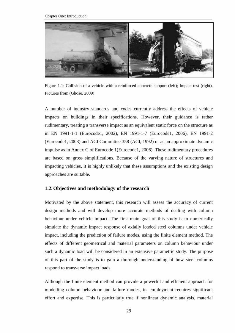
Underground and multi-storey car parks’ columns, ground floor columns in buildings
located along busy roads and bridge pairs are highly vulnerable to impact loads due to
moving vehicles (see Fig. 1.1). The failure of these supporting structures, as a result of
impact, may lead to progressive collapse. Therefore, a proper analysis technique is
required. This analysis technique should be suitable for routine structural design so that
this mode of failure can be dealt with by a majority of engineers. Despite extensive past
research on structural behaviour under impact, the behaviour of columns under extreme
loading conditions is still not well understood.
Chapter One: Introduction
29
Figure 1.1: Collision of a vehicle with a reinforced concrete support (left); Impact test (right).
Pictures from (Ghose, 2009)
A number of industry standards and codes currently address the effects of vehicle
impacts on buildings in their specifications. However, their guidance is rather
rudimentary, treating a transverse impact as an equivalent static force on the structure as
in EN 1991-1-1 (Eurocode1, 2002), EN 1991-1-7 (Eurocode1, 2006), EN 1991-2
(Eurocode1, 2003) and ACI Committee 358 (ACI, 1992) or as an approximate dynamic
impulse as in Annex C of Eurocode 1(Eurocode1, 2006). These rudimentary procedures
are based on gross simplifications. Because of the varying nature of structures and
impacting vehicles, it is highly unlikely that these assumptions and the existing design
approaches are suitable.
1.2. Objectives and methodology of the research
Motivated by the above statement, this research will assess the accuracy of current
design methods and will develop more accurate methods of dealing with column
behaviour under vehicle impact. The first main goal of this study is to numerically
simulate the dynamic impact response of axially loaded steel columns under vehicle
impact, including the prediction of failure modes, using the finite element method. The
effects of different geometrical and material parameters on column behaviour under
such a dynamic load will be considered in an extensive parametric study. The purpose
of this part of the study is to gain a thorough understanding of how steel columns
respond to transverse impact loads.
Although the finite element method can provide a powerful and efficient approach for
modelling column behaviour and failure modes, its employment requires significant
effort and expertise. This is particularly true if nonlinear dynamic analysis, material
Chapter One: Introduction
30
nonlinearity and strain rate dependence are included. Furthermore, in many situations,
obtaining finite element solutions requires a considerable amount of computation time
which prevents its use during routine design. Therefore, the second main goal of this
research is to develop a simplified analytical or semi-analytical approach that can be
used to predict the critical impact velocity of vehicle impact on axially loaded steel
columns. This proposed method will utilize the energy balance approach assuming
quasi-static behaviour for the impacted steel column. Based on the aforementioned two
goals, the detailed objectives are as follows:
1. To suggest and validate a numerical model for simulating axially loaded steel
columns subjected to transverse impact using the commercial finite element
code ABAQUS/Explicit. The validation should be based on a comparison
between the proposed simulation model and relevant experiments;
2. To conduct extensive parametric study to provide a comprehensive database of
results covering different impact masses, impact velocities and impact locations
in addition to different column boundary conditions, axial load ratios and section
sizes. The numerical simulation results will also be used to develop an
understanding of the detailed behaviour of steel columns under transverse
impact in order to inform the assumptions of the proposed analytical method;
3. To develop a simplified numerical vehicle model which can be used to simulate
the effects of vehicle impact on steel columns by using the commercial finite
element code ABAQUS/Explicit without having to use a full scale numerical
vehicle model;
4. To develop and validate a simplified analytical method for predicting the critical
impact velocities of vehicle impact on axially compressed steel columns.
5. To use the numerical simulation results to assess the accuracy of the current
Eurocode 1 design methods.
1.3. Layout of the thesis
This thesis presents the detailed results of the author’s work over a three year PhD
research programme which was aimed at achieving the objectives of the research. It
includes a detailed literature review of the different aspects of the research project, a

Chapter One: Introduction
31
validation of the numerical simulations, an extensive parametric study and the
development of the analytical approach. The thesis is divided into the following nine
chapters.
Chapter one: Presents an introduction of the research problem with a statement of the
objectives and aims of the research.
Chapter two: Reviews the previous studies relevant to the research problem in addition
to the approaches suggested in the current design codes of practice. The main focus of
this chapter is to present and discuss the previous research studies in this field so as to
identify gaps in knowledge in order to justify the originality of this research and to
formulate an appropriate research methodology for this research.
Chapter three: Presents a detailed description of the techniques used in numerical
simulations to model the transverse impact problem of axially compressed columns
using the finite element code ABAQUS/Explicit. It will also describe the geometrical,
material, and loading application parameters used in the numerical model. The chapter
will present the numerical simulations of relevant tests and compare the numerical
simulation results against tests’ results.
Chapter four: Presents the parametric study conducted based on the numerical model
validated in chapter three to investigate the effects of several parameters on the response
of axially loaded steel columns. The chapter discusses the parametric study results and
ends up with important conclusions, based on which simplifying assumptions on
column behaviour under impact can be made to develop appropriate design calculation
methods.
Chapter five: Presents and validates a simplified numerical vehicle model that can be
used to simulate the effects of vehicle frontal impact on steel columns. The simplified
numerical vehicle model treats the vehicle as a spring-mass system. The chapter also
presents the derivations and validation of a simplified equation to predict the equivalent
linear stiffness of a vehicle that can be used in the simplified analytical model.

Chapter One: Introduction
32
Chapter six: Presents the development of a simplified analytical method to predict the
critical velocities of transverse impact on steel columns under axial load. This method is
based on an energy balance assuming a quasi-static approximation of column
behaviour.
Chapter seven: Validates the accuracy of the proposed simplified analytical method
presented in chapter six by comparison against numerical simulation results using
ABAQUS/Explicit.
Chapter eight: Evaluates the accuracy of the design requirements suggested by the
current Eurocode 1, based on the numerical simulation results.
Chapter nine: Presents the main findings and conclusions of the research with
suggestions for future research work.

Chapter Two: Literature Review
33
Chapter Two
Literature Review
2.1. The research problem Civil engineering structures are frequently being subjected to various types of transverse
dynamic impact loads. The following impact events may cause significant damage to
structures and they should be included in the structural design of structural members
that are prone to such events.
1. Transverse impact caused by ships or vehicles on bridge piers (El-Tawil et al., 2005,
Sharma et al., 2012), see Fig. 2.1;
2. Transverse impact caused by travelling vehicles on buildings situated near busy roads
(Ellis, 2003), see Fig. 2.2;
3. Transverse impact caused by travelling vehicles on traffic light or lighting poles
(Elmarakbi et al., 2006, Klyavin et al., 2008), (see Fig. 2.3) and on road safety barriers
(Jiang et al., 2004).
4. Transverse impact caused by moving vehicles on ground floor columns of multi-
storey car parks (Ferrer et al., 2010),
5. Transverse impact caused by aeroplanes on multi-storey buildings or skyscrapers.
Figure 2.1: Collapse of a bridge after being struck by tractor-trailer (courtesy of NDOR) (El-Tawil et al., 2005)
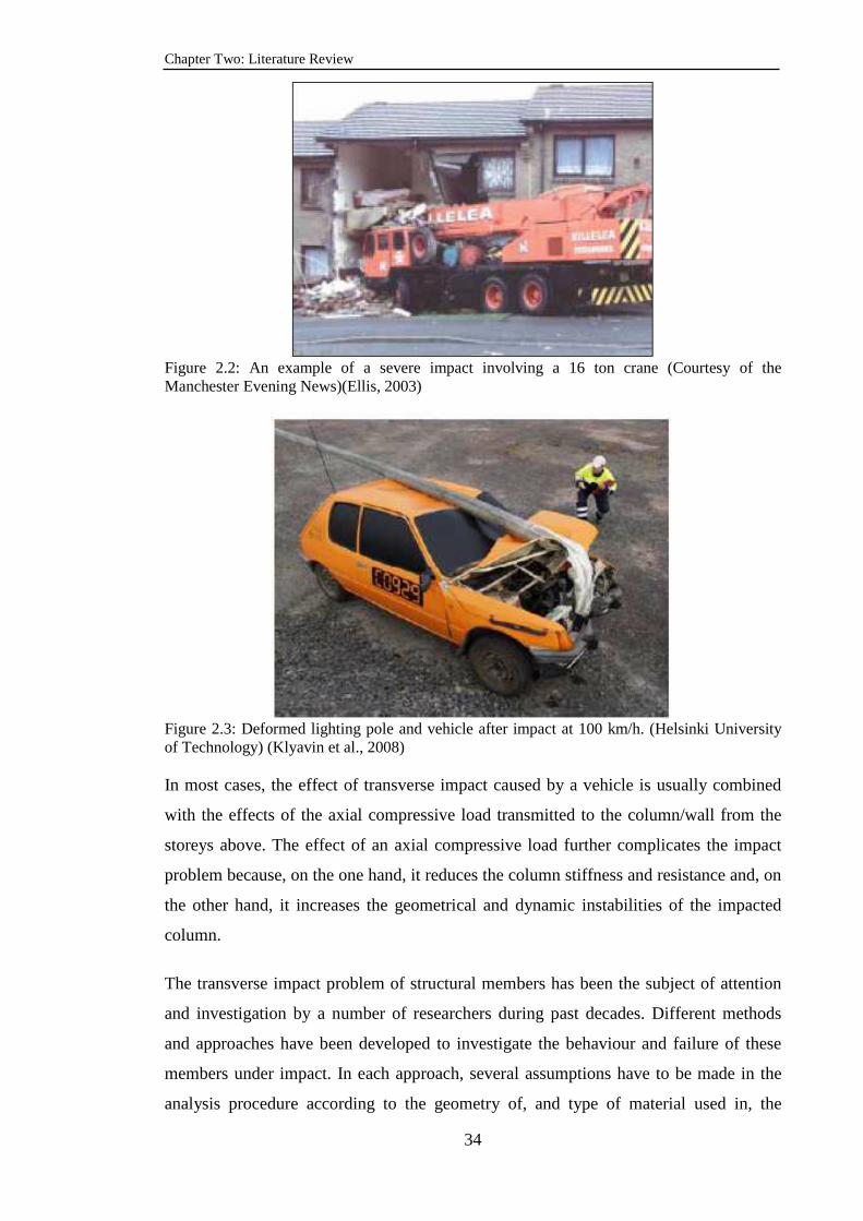
Chapter Two: Literature Review
34
Figure 2.2: An example of a severe impact involving a 16 ton crane (Courtesy of the Manchester Evening News)(Ellis, 2003)
Figure 2.3: Deformed lighting pole and vehicle after impact at 100 km/h. (Helsinki University of Technology) (Klyavin et al., 2008) In most cases, the effect of transverse impact caused by a vehicle is usually combined
with the effects of the axial compressive load transmitted to the column/wall from the
storeys above. The effect of an axial compressive load further complicates the impact
problem because, on the one hand, it reduces the column stiffness and resistance and, on
the other hand, it increases the geometrical and dynamic instabilities of the impacted
column.
The transverse impact problem of structural members has been the subject of attention
and investigation by a number of researchers during past decades. Different methods
and approaches have been developed to investigate the behaviour and failure of these
members under impact. In each approach, several assumptions have to be made in the
analysis procedure according to the geometry of, and type of material used in, the

Chapter Two: Literature Review
35
structure under consideration; the dynamic characteristics of the impacting body (impact
velocity, impact duration, impact mass); the deformations expected to develop during
the short period of the impact event; and the failure mode which either involves local
failure or the geometrical instability of the whole structural member. However, as will
be discerned from the following literature review, research on this specific topic is still
rudimentary and lacks sufficient depth and detail to inform the design process.
It is the aim of this chapter to present and discuss previous research studies relating to
the above mentioned impact problem in order to assist in gaining a clearer
understanding of the behaviour and failure modes of axially loaded steel columns under
vehicle impact. The discussions will focus on the main assumptions used in these
studies and the main findings reached, and how they can be incorporated in the
methodology used in the present study.
2.2. Current codes of practice A number of current industry standards and codes of practice include rudimentary
guidance on how to address the effects of vehicle impact on buildings (Eurocode1,
2002, Eurocode1, 2006, ACI, 1992) and bridge structures (Eurocode1, 2003, Highways
Agency, 2004, AASHTO, 2007) by treating the transverse impact as an equivalent static
force on the structure. For example, the informative Annex B of Eurocode1: Part1-1
(Eurocode1, 2002) suggests the following simple and general equation, to calculate the
design horizontal characteristic force on barriers in car parks to withstand the impact of
a vehicle:
2.
2( )r
c b
M vF
δ δ=
+ ................................................................................................................................... 2.1
Where M is the total mass of the vehicle, vr is velocity of the vehicle normal to the
impacted structure, cδ is deformation of the vehicle, bδ is the deformation of the
impacted structure.
Conceptually, this equation (Eq. 2.1) is easily derived based on conservation of energy
in the system before and after the impact, but it assumes plastic force-displacement
response for both the barrier and the impacting vehicle. The impact energy of the
vehicle (0.5Mv2r) is assumed to be entirely absorbed by the plastic deformation of the
vehicle ( cδ ) and the structure (bδ ) which have a force (F) at the interface between the

Chapter Two: Literature Review
36
two. According to this Annex, the maximum impact velocity at which the equation is
valid is 4.5m/s (16.2km/h) and the maximum vehicle deformation is 100mm
(Eurocode1, 2002).
Sections 4.3 and 4.4 of Eurocode1: Part1-7 (Eurocode1, 2006) define the accidental
action due to impact from vehicles and forklift trucks respectively. Section 4.3
recommends that impact may be represented by an equivalent static force giving the
equivalent dynamic action effects on the structures. The design values of the equivalent
static force are given in two tables as constant values corresponding to each category of
traffic. Each table represents a particular kind of structure, namely supporting-structures
and super-structures, see Table 2.1 and Table 2.2. In both tables, the effects of vehicle
mass, vehicle velocity and vehicle stiffness characteristics, in addition to those of the
impacted structure are all ignored.
Table 2.1: Indicative equivalent static design forces due to vehicular impact on members supporting structures over, or adjacent to, roadways, (Eurocode1, 2006)
Category of traffic Force Fadx
(kN) Force Fa
dy (kN)
Motorways and country national and main roads
1000* 500
Country roads in rural area 700 375 Roads in urban area 500 250 Courtyards and parking garages with access to: - Cars - Lorriesb
50 150
25 75
a x= direction of normal travel, y = perpendicular to the direction of normal travel. b The term “lorry” refers to vehicles with a maximum gross weight greater than 3.5 tonnes.
Table 2.2: Indicative equivalent static design forces due to impact on superstructures (Eurocode1, 2006)
Category of traffic Equivalent static design force Fadx
(kN) Motorways and country national and main roads
500
Country roads in rural area 375 Roads in urban area 250 Courtyards and parking garages 75 a x = direction of normal travel
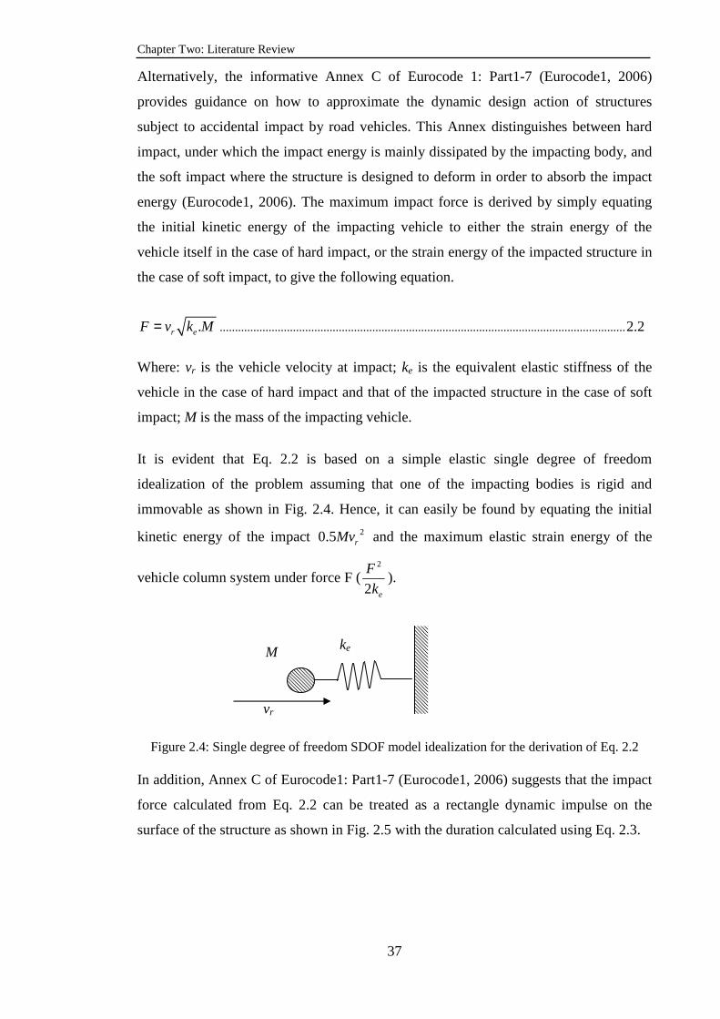
Chapter Two: Literature Review
37
Alternatively, the informative Annex C of Eurocode 1: Part1-7 (Eurocode1, 2006)
provides guidance on how to approximate the dynamic design action of structures
subject to accidental impact by road vehicles. This Annex distinguishes between hard
impact, under which the impact energy is mainly dissipated by the impacting body, and
the soft impact where the structure is designed to deform in order to absorb the impact
energy (Eurocode1, 2006). The maximum impact force is derived by simply equating
the initial kinetic energy of the impacting vehicle to either the strain energy of the
vehicle itself in the case of hard impact, or the strain energy of the impacted structure in
the case of soft impact, to give the following equation.
.r eF v k M= ..................................................................................................................................... 2.2
Where: vr is the vehicle velocity at impact; ke is the equivalent elastic stiffness of the
vehicle in the case of hard impact and that of the impacted structure in the case of soft
impact; M is the mass of the impacting vehicle.
It is evident that Eq. 2.2 is based on a simple elastic single degree of freedom
idealization of the problem assuming that one of the impacting bodies is rigid and
immovable as shown in Fig. 2.4. Hence, it can easily be found by equating the initial
kinetic energy of the impact 20.5 rMv and the maximum elastic strain energy of the
vehicle column system under force F (2
2 e
F
k).
Figure 2.4: Single degree of freedom SDOF model idealization for the derivation of Eq. 2.2
In addition, Annex C of Eurocode1: Part1-7 (Eurocode1, 2006) suggests that the impact
force calculated from Eq. 2.2 can be treated as a rectangle dynamic impulse on the
surface of the structure as shown in Fig. 2.5 with the duration calculated using Eq. 2.3.
M ke
vr
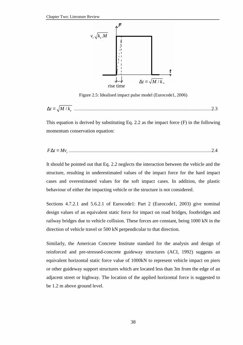
Chapter Two: Literature Review
38
Figure 2.5: Idealised impact pulse model (Eurocode1, 2006)
/ et M k∆ = ..................................................................................................................................... 2.3
This equation is derived by substituting Eq. 2.2 as the impact force (F) in the following
momentum conservation equation:
rF t Mv∆ = .......................................................................................................................................... 2.4
It should be pointed out that Eq. 2.2 neglects the interaction between the vehicle and the
structure, resulting in underestimated values of the impact force for the hard impact
cases and overestimated values for the soft impact cases. In addition, the plastic
behaviour of either the impacting vehicle or the structure is not considered.
Sections 4.7.2.1 and 5.6.2.1 of Eurocode1: Part 2 (Eurocode1, 2003) give nominal
design values of an equivalent static force for impact on road bridges, footbridges and
railway bridges due to vehicle collision. These forces are constant, being 1000 kN in the
direction of vehicle travel or 500 kN perpendicular to that direction.
Similarly, the American Concrete Institute standard for the analysis and design of
reinforced and pre-stressed-concrete guideway structures (ACI, 1992) suggests an
equivalent horizontal static force value of 1000kN to represent vehicle impact on piers
or other guideway support structures which are located less than 3m from the edge of an
adjacent street or highway. The location of the applied horizontal force is suggested to
be 1.2 m above ground level.
.r ev k M
/ et M k∆ = rise time
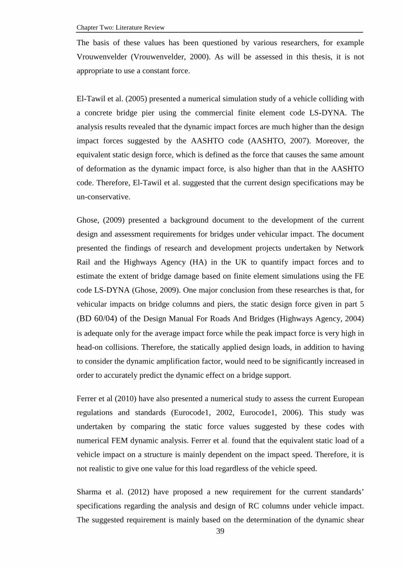
Chapter Two: Literature Review
39
The basis of these values has been questioned by various researchers, for example
Vrouwenvelder (Vrouwenvelder, 2000). As will be assessed in this thesis, it is not
appropriate to use a constant force.
El-Tawil et al. (2005) presented a numerical simulation study of a vehicle colliding with
a concrete bridge pier using the commercial finite element code LS-DYNA. The
analysis results revealed that the dynamic impact forces are much higher than the design
impact forces suggested by the AASHTO code (AASHTO, 2007). Moreover, the
equivalent static design force, which is defined as the force that causes the same amount
of deformation as the dynamic impact force, is also higher than that in the AASHTO
code. Therefore, El-Tawil et al. suggested that the current design specifications may be
un-conservative.
Ghose, (2009) presented a background document to the development of the current
design and assessment requirements for bridges under vehicular impact. The document
presented the findings of research and development projects undertaken by Network
Rail and the Highways Agency (HA) in the UK to quantify impact forces and to
estimate the extent of bridge damage based on finite element simulations using the FE
code LS-DYNA (Ghose, 2009). One major conclusion from these researches is that, for
vehicular impacts on bridge columns and piers, the static design force given in part 5
(BD 60/04) of the Design Manual For Roads And Bridges (Highways Agency, 2004)
is adequate only for the average impact force while the peak impact force is very high in
head-on collisions. Therefore, the statically applied design loads, in addition to having
to consider the dynamic amplification factor, would need to be significantly increased in
order to accurately predict the dynamic effect on a bridge support.
Ferrer et al (2010) have also presented a numerical study to assess the current European
regulations and standards (Eurocode1, 2002, Eurocode1, 2006). This study was
undertaken by comparing the static force values suggested by these codes with
numerical FEM dynamic analysis. Ferrer et al. found that the equivalent static load of a
vehicle impact on a structure is mainly dependent on the impact speed. Therefore, it is
not realistic to give one value for this load regardless of the vehicle speed.
Sharma et al. (2012) have proposed a new requirement for the current standards’
specifications regarding the analysis and design of RC columns under vehicle impact.
The suggested requirement is mainly based on the determination of the dynamic shear
Chapter Two: Literature Review
40
resistance of the column to prevent a certain level of damage to occur in the column
rather than to prevent the column collapse mechanism as currently suggested by most of
the current standard and codes. It has been found that the column dynamic shear
resistance varies with the mass and velocity of the vehicle in addition to the column
configuration. Moreover, it has been concluded that the estimated values of dynamic
shear force is greater that the static or quasi-static quantity currently suggested by most
of the codes of practice. Therefore, the study suggests that the dynamic resistance must
be used for the analysis and design of structures subjected to vehicle impact.
It is clear from the previous discussions that although representing the transverse impact
as an equivalent static force, or using a dynamic impulse approximation as in the current
standards and codes, may provide design engineers with a relatively simple empirical
design or assessment procedure; it involves many uncertainties that may be grossly
inaccurate. For instance, none of the above methods considers the interactions between
the structure and the impacting body. In addition, none of the above methods includes
work undertaken by the axial force in the structural member as it deforms. Also the
existing research studies have focused on bridge support structures and there is a lack of
such investigation for building structures. The main objective of the present study is to develop a more realistic analysis procedure
to predict the dynamic impact effects and to quantify the failure conditions of axially
loaded steel columns under a transverse vehicle impact. Different parameters will be
considered in the analysis including column boundary conditions, column axial load
ratios, vehicle masses, vehicle velocities and impact locations and directions. The
behaviour and failure of the impacted column under such a dynamic event will be
predicted numerically and analytically in terms of the critical impact velocity at which
the column would be considered to have failed. Both global and local failure modes will
be included in the numerical analysis. 2.3. Previous research studies Due to resource limitation, this study will be conducted numerically and analytically.
The numerical results will be used to generate extensive data for developing the
analytical methods. The numerical simulations will need to be validated by comparison
against the experimental results obtained by others. Thus, it is necessary to review the
Chapter Two: Literature Review
41
developments related to steel column behaviour under transverse impact and the
analytical methods used to predict such dynamic behaviour.
In addition, this research is concerned with steel columns under vehicle impact and it is
not desirable to introduce a detailed simulation of the vehicle when studying the column
behaviour. Therefore, simplification of the vehicle is required and this chapter will also
provide a review on vehicles characterises used in this simplifications.
2.3.1. Behaviour and failure modes of axially compressed columns under a transverse impact load
A considerable amount of literature has been published on the experimental and
numerical studies of the behaviour and failure modes of structural members under
transverse impact. In particular, the behaviour of axially restrained beams under
transverse impact has been studied intensively (Menkes and Opat, 1973, Liu and Jones,
1987, Yu and Jones, 1989, Yu and Jones, 1991, Yu and Jones, 1997, Mannan et al.,
2008, Bambach et al., 2008). This is understandable as axially restrained beams are
frequently used as members to absorb impact energy in such major applications as
vehicle crash barriers. On the other hand, although columns under compressive load
may also be involved in an accidental vehicle crash, the emphasis has been almost
wholly on vehicle crashworthiness for occupant protection. However, with structural
robustness now an important topic for the structural engineering research community,
the behaviour of columns under vehicle impact deserves attention. Nevertheless,
although the behaviour of axially compressed columns under transverse impact will be
different from that of axially restrained beams undergoing axial tension, a review of
beam behaviour can help to understand some aspects of the steel column behaviour.
The experimental study of Menkes and Opat (1973) identified three modes of failure of
clamped aluminium beams subjected to transverse impulsive dynamic load. These
failure modes essentially depended on the impulse intensity (see Fig. 2.6)
I- large plastic deformation of the whole beam with the formation of a plastic
hinge mechanism;
II- tensile tearing failure under catenary action, and
III- transverse shear failure at the supports.
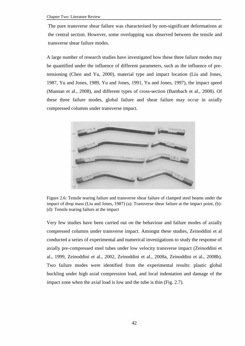
Chapter Two: Literature Review
42
The pure transverse shear failure was characterised by non-significant deformations at
the central section. However, some overlapping was observed between the tensile and
transverse shear failure modes.
A large number of research studies have investigated how these three failure modes may
be quantified under the influence of different parameters, such as the influence of pre-
tensioning (Chen and Yu, 2000), material type and impact location (Liu and Jones,
1987, Yu and Jones, 1989, Yu and Jones, 1991, Yu and Jones, 1997), the impact speed
(Mannan et al., 2008), and different types of cross-section (Bambach et al., 2008). Of
these three failure modes, global failure and shear failure may occur in axially
compressed columns under transverse impact.
Figure 2.6: Tensile tearing failure and transverse shear failure of clamped steel beams under the impact of drop mass (Liu and Jones, 1987) (a): Transverse shear failure at the impact point, (b)-(d): Tensile tearing failure at the impact
Very few studies have been carried out on the behaviour and failure modes of axially
compressed columns under transverse impact. Amongst these studies, Zeinoddini et al
conducted a series of experimental and numerical investigations to study the response of
axially pre-compressed steel tubes under low velocity transverse impact (Zeinoddini et
al., 1999, Zeinoddini et al., 2002, Zeinoddini et al., 2008a, Zeinoddini et al., 2008b).
Two failure modes were identified from the experimental results: plastic global
buckling under high axial compression load, and local indentation and damage of the
impact zone when the axial load is low and the tube is thin (Fig. 2.7).

Chapter Two: Literature Review
43
Figure 2.7: View of the deformed specimens after impact (Zeinoddini et al., 2002)
Adachi et al (2004) and Sastranegara et al. (2005) investigated experimentally and
numerically the buckling and post buckling behaviour of a number of small scale axially
compressed aluminium columns subjected to lateral impact loads. They also identified
global instability as the main failure mode of the columns, see Fig. 2.8. Due to the
failure mode being global buckling, they found that the critical condition of column
buckling was controlled only by the kinetic energy of the transverse impact, but was
independent of the history of the transverse impact or its impulse. It has been observed
that when a column is subjected to transverse impact, it buckles in the lower bucking
mode under pure axial load irrespective of the location of impact.
Figure 2.8: Buckling failure of impacted aluminium columns for different impact velocities (Adachi et al., 2004)
Typically, as the above studies were among the first on this topic, they are limited in
scope and their conclusions are preliminary. Consequently, there is insufficient data to
Chapter Two: Literature Review
44
develop comprehensive understanding of the effects of various parameters on steel
column behaviour for the development of practical design methods. The aim of this
research is to build on these preliminary research investigations and to develop an
extensive database of column behaviour under transverse impact. Some of the above
mentioned experimental results also provide data for the validation of the numerical
modelling presented in chapter three.
As a summary, the following failure modes are the ones most likely to occur in axially
loaded steel columns under transverse impact:
a) Shear failure (either at the impact zone or at the supports)
b) Local failure and indentation at the impact zone, and
c) Global buckling of the whole impacted column.
This research will attempt to identify the conditions under which these failure modes
occur and to focus attention on the most relevant failure mode, i.e. global buckling.
2.3.2. Analytical research studies
Although the finite element method can provide an accurate and versatile approach for
modelling structural behaviour under impact, its employment requires significant effort
and expertise. This is particularly true if nonlinear dynamic analysis, material
nonlinearity and strain rate dependence are included in the numerical simulations.
Moreover, in many situations, obtaining such a complex finite element solution
consumes a great amount of computation time, which precludes its use in general
structural design. It is, therefore, desirable to develop an approximate, but simplified
analytical method.
This section will present a detailed review and description of a number of selected
analytical researches that are directly relevant to the present research study, and which
will later be used as background for developing the analytical or semi-analytical
modelling approach, to be reported in detail in chapter six.
Developing a simplified method for analysing structural response under impact load has
received significant research effort (Parkes, 1958, Symonds and Mentel, 1958, Nonaka,
1967, Symonds and Jones, 1972, Liu and Jones, 1988, Jones, 1997, Chen and Yu,
2000). However, as in the experimental studies, these investigations have all

Chapter Two: Literature Review
45
concentrated on beam or plate structures under pure bending or axial tension (when
axially restrained) under impact.
The quasi-static approach was also adopted in the development of the analytical
methods. In this approach, the static equilibrium state is assumed for the structural
system and the resultant static deformation shape is then used to express the energy
absorbed due to the elastic and/or plastic deformations of the impacted structural
member. The equation of the external work done by the axial load can also be derived
based on the assumed static deformation shape. The static deformation shape could be
assumed to be the deformation shape of the structural member under transverse loads
(Biggs, 1964, Humar, 2002), or the buckling mode shape of the column (Adachi et al.,
2004, Sastranegara et al., 2006, Shope, 2006). Afterwards, the energy quantities are
used to write the energy conservation equation for the original dynamic system.
Experimental validation of the quasi-static assumption was provided by Liu and Jones
(1987) who conducted tests on small scale clamped metal beams impacted transversely
by a rigid mass travelling with low impact velocities at different locations along the
beam length. They revealed that the locations and types of failure of the impacted
beams were similar to those of the beams loaded statically. This is an important
conclusion which can be employed to simplify the analytical approaches to beams and
columns under such transverse impacts. Further experimental and numerical
confirmations of the quasi-static assumption may be traced to Zeinoddini et al (2002,
Zeinoddini et al., 2008a) who, crucially, indicated that quasi-static analysis may be used
for the impact velocity used (25.9 km/h).
The analytical study undertaken by Jones (Jones, 1995) on a clamped beam has shown
that the quasi-static analysis can be used to predict the inelastic behaviour of clamped
beams subjected to low velocity transverse impact provided that the ratio of the striker
mass to the beam mass is not less than one in order to ensure that most of the impact
kinetic energy would be absorbed as plastic deformations during the global plastic
mechanism phase. A comparison between the quasi-static solution results with the
theoretical dynamic solution obtained by Shen and Jones (1991) has revealed that the
error introduced by the quasi-static procedure was within acceptable ranges provided
that the ratio of the striker mass to the beam mass is larger than about three. The error is
significant when the striker masses are smaller than the total beam mass. It has also
been concluded that, for many engineering applications, the rigid-plastic assumption of

Chapter Two: Literature Review
46
the material behaviour may be used to simplify the quasi-static analysis. Even in the
case of a light vehicle impacting a heavy steel column section, it is expected that the
ratio of the vehicle mass to the steel column mass will not be less than one. Therefore,
the quasi-static assumption can be adopted for the research problem of this study.
The quasi-static method has also been adopted by Wen et al (1995) and Bambach et al.
(2008) to establish the transverse force - transverse displacement relationship. In the
Wen et al. study (1995) an analytical method was presented to predict the critical
transverse deformations, the critical absorbed energy and failure modes of the clamped
beam made from a rigid –perfectly plastic material subjected to transverse impact by a
mass travelling at a low velocity. The quasi-static approximation has been adopted in
the analysis to derive the force-displacement relationship using a virtual work method.
The plastic deformation shape was assumed in order to derive the transverse and axial
deformations’ relationships. As the clamped beam is more vulnerable to shear and
membrane action effects, both deformations were included in deriving the force-
displacement relationship alongside the bending deformations. The energy conservation
principle was then employed to determine the maximum plastic transverse deformation
at which the steel beam failure occurs under both tensile tearing and/or shear failure
modes. The comparison with the experimental results confirmed the validity of the
proposed method.
Bambach et al. (2008) used the quasi-static method to establish the transverse force -
transverse displacement relationship of hollow and concrete filled steel beam sections
under transverse impact using a procedure similar to that adopted by Jones (1995),
taking into account the effect of the local reduction in the sectional depth at the impact
point on the plastic moment capacity of the section at that point by applying the
interaction curve equation for this type of steel sections, (see Fig.2.9).
Figure 2.9: Theoretical model of Bambach et al. (2008)

Chapter Two: Literature Review
47
The present study aims to address the problem of axially compressed steel columns
under transverse impact on which there is very little research. The presence of an axial
compressive load significantly changes the behaviour of the structural member and
failure mode, from local or shear failure of structural beams/plates with in-plane axial
restraint to global buckling failure under compression. Among a few relevant research
studies, Shope (Shope, 2006) has used the energy conservation principle with quasi-
static approximation to develop a simplified analytical and design model to predict the
critical impulse values for a wide flanged steel column section (W8x4) under a static
axial force subjected to a blast load with different boundary conditions and slenderness
ratios. In that study, Shope assumed that the system behaves as a single degree of
freedom in an elastic perfectly plastic manner, as shown in Fig. 2.10. The critical
impulse-axial load relationship was obtained by setting the kinetic energy of the
impulse equal to the total strain energy of the column at the maximum plastic
displacement point. Since the numerical model utilized a beam element to model the
steel column, the effect of local deformation or flange buckling was not considered in
both the numerical simulations and the suggested analytical method.
Figure 2.10: Idealized system used by Shope (2006) with elastic–perfectly plastic material behaviour Tsang and Lam (2008) have employed the quasi–static nonlinear approach combined
with the energy conservation principle to investigate the impact resistance of reinforced
concrete columns subjected to road vehicle impact at the column mid-height. The
impact resistance of the column was estimated by determining the frontal impact
velocity of the vehicle to cause global instability of the column. The energy absorbed by
the column at failure was used in the energy balance equation. The transverse impact
force resistance function was derived based on a quasi-static approximation of the
reinforced concrete column behaviour under the dynamic impact load (Fig. 2.11).
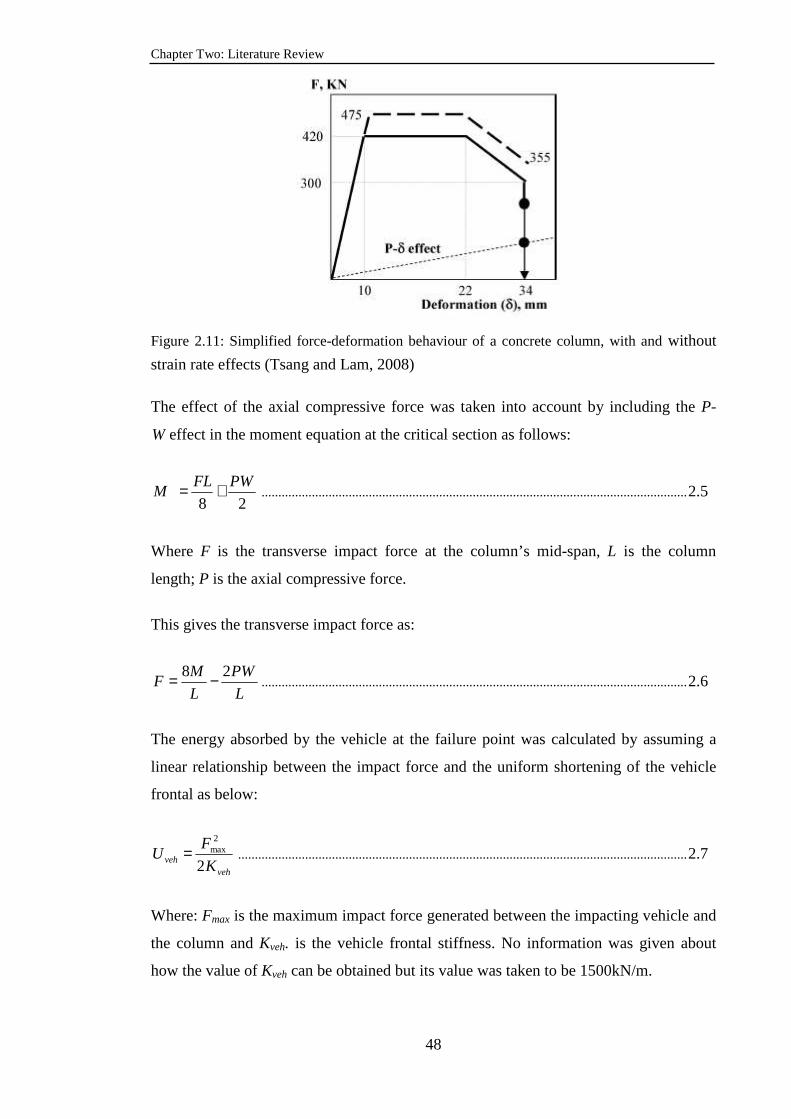
Chapter Two: Literature Review
48
Figure 2.11: Simplified force-deformation behaviour of a concrete column, with and without
strain rate effects (Tsang and Lam, 2008)
The effect of the axial compressive force was taken into account by including the P-
W effect in the moment equation at the critical section as follows:
8 2
FL PWM = + ............................................................................................................................... 2.5
Where F is the transverse impact force at the column’s mid-span, L is the column
length; P is the axial compressive force.
This gives the transverse impact force as:
8 2M PW
FL L
= − ............................................................................................................................... 2.6
The energy absorbed by the vehicle at the failure point was calculated by assuming a
linear relationship between the impact force and the uniform shortening of the vehicle
frontal as below:
vehveh K
FU
2
2max= ...................................................................................................................................... 2.7
Where: Fmax is the maximum impact force generated between the impacting vehicle and
the column and Kveh. is the vehicle frontal stiffness. No information was given about
how the value of Kveh can be obtained but its value was taken to be 1500kN/m.
Chapter Two: Literature Review
49
A comparison with non-linear dynamic simulation results showed that the quasi-static
method underestimated the column impact resistance by 40%. This underestimation of
column resistance was as a result of neglecting the contribution of the inertia force on
the column resistance (Tsang and Lam, 2008). However, for steel columns that are
much lighter in weight than RC columns, the effects of the inertial force will be small
and it may acceptable to discard them.
It is evident from the aforementioned literature review that there are gross assumptions
in the design of axially loaded steel columns under transverse impact. Therefore, one of
the main objectives of this research is to present the full development of an analytical
method for predicting the critical velocity of vehicle impact on steel columns under
axial compression that may be adopted in design. This proposed method will utilize the
energy balance approach assuming quasi-static behaviour of the impacted steel column.
The steel stress-strain curve will be assumed to be elastic-perfectly plastic. The energy
balance approach will account for both elastic and plastic lateral deformations of the
steel column, axial movement of the column and the energy absorbed by vehicle
deformations.
2.3.3. Vehicle characteristics
Many research studies have used the finite element method to simulate vehicle impact
on structures. In some of these studies, the vehicle impact was simulated using a time
varying load with an assumed maximum amplitude (Thilakarathna et al., 2010, Varat
and Husher, 2000 ) as shown in Fig. 2.12. The impact load-time function of the vehicle
may be obtained from experimental crash tests. However, this approach involves many
approximations and uncertainties which affect the level of accuracy achieved. For
example, the impact force-time history of the vehicle cannot be accurately predicted
because it depends on a large number of variables including the vehicle dynamic
characteristics such as vehicle mass, vehicle velocity and the strain rate sensitivity of
vehicle components (see Fig. 2.12(B)) in addition to the geometrical and material
characteristics of the impacted column itself. Moreover, this approach cannot accurately
account for the local deformations in the vehicle at the impact point because it does not
simulate the contact interaction generated between the vehicle and the column.
Furthermore, the effect of kinetic impact energy on column behaviour and failure
cannot be considered if the vehicle impact is input as an impulsive load.

Chapter Two: Literature Review
50
A B
Figure 2.12: (A) A frontal collision test of a Honda Accord at a speed of 48.3 km/h;(B) Force-
time histories of full scale crash tests for different types of vehicle (from (Thilakarathna et al.,
2010).
On the other hand, full-scale finite element models of vehicles have been frequently
used to simulate vehicle impact under different impact scenarios to assess vehicle
integrity. Full scale vehicle modelling is necessary because the focus is on the vehicle.
However, the simulation is demanding, involving a very large number of elements,
material nonlinearity, strain rate dependency and very large strains and deformations.
For structural engineering applications of vehicle impact on structural members such as
the columns of a building, it is doubtful whether full-scale vehicle modelling is
necessary when the focus of the study is on the structural member, not the vehicle.
Nevertheless, some numerical studies have been attempted using full-scale numerical
vehicle models to assess the design approaches and equations used to investigate
vehicle impact on columns and bridge piers under vehicle impact. These studies include
a numerical study of vehicle impact on concrete bridge piers conducted by El-Tawil et
al. (2005), a numerical study of vehicle impact on a traffic light steel pole by Elmarakbi
et al. (2006) and the numerical study conducted by Ferrer et al. (2010) to simulate
vehicle impact on underground car park steel columns. In all these studies, some
limitations had to be applied in order to reduce the simulation effort and time. For
example, in the El-Tawil et al. study, the effects of material nonlinearity and the failure
of the structure were neglected and in the Elmarakbi et al. and Ferrer et al. studies,
material failure was also neglected in the simulation and only one direction of impact
was considered in the numerical simulations. These limitations severely restrict the
applications of such investigations. Furthermore, in many situations, a full-scale model
of a particular vehicle type is either not yet available or is not accessible to engineers.
0.0E+00
1.0E+05
2.0E+05
3.0E+05
4.0E+05
5.0E+05
6.0E+05
7.0E+05
0 0.02 0.04 0.06 0.08 0.1 0.12
Time (sec.)
Impa
ct F
orce
(N
)
Ford Tautus; V=56km/h,
mass=1619kgHonda Accord;V=48km/h, mass=1329kgRenault Fuego;V=48km/h, mass=1329kg

Chapter Two: Literature Review
51
The above discussion leads to the conclusion that there is a need to develop a simplified
numerical vehicle model which can be utilized for studying the behaviour and failure of
structures under vehicle impact. This has already been recognized by others and the
following sections review work already undertaken in this area to identify the gap for
further development.
2.3.3.1. Simplifying approaches
Based on an experimental study of vehicle frontal collision on a rigid barrier, Emori
(Emori, 1968) suggested that the undamaged or intact portion of the impacting vehicle
may be considered as a rigid body while the crushed portion of the vehicle absorbs all
the kinetic energy of the impacting vehicle just before the impact. Therefore, the vehicle
impact processes may be modelled by a spring-mass system in which the rigid mass
represents the vehicle total mass and the one-way linear spring represents the vehicle
resistance, see Fig.2.13.
Figure 2.13: Spring-mass system used by Emori (Emori, 1968).
Tani and Emori (1970) proposed a more sophisticated mathematical model having three
masses and three springs simulating the three parts of a vehicle: the engine box, the
structure in front of the engine and the frontal structure. The load-deflection
characteristics of each spring were determined based on experimental observations.
Kamal (1970) and Lin (1973) proposed further refinements to the previous two models
by using eight nonlinear springs with three masses to simulate frontal impact (Kamal,
1970) and seven nonlinear springs to simulate rear barrier impact (Lin, 1973).
In the above-mentioned studies, the vehicle impact was against a wide, flat and rigid
barrier rather than a deformable structure with a limited width such as a column
considered in the present study. Nevertheless, the concept of simplifying the vehicle

Chapter Two: Literature Review
52
using a spring-mass system is still applicable as long as the spring can capture the
dynamic and stiffness characteristics of the impacting vehicle.
Milner et al. (2001) presented a simplified theoretical study based on the dynamic
analysis of two and three degrees of freedom system of a vehicle impacting on wooden
poles. In their analytical model, the vehicle was modelled by a mass representing the
vehicle total mass and a bi-linear stiffness representing the vehicle stiffness
characteristics before and after the engine location, see Fig. 2.14. No information was
given in the study about how the bilinear stiffness values were obtained. However, their
validation results suggested validity of the bilinear stiffness assumption.
Figure 2.14: Vehicle stiffness characteristics defined by Milner et al. (Milner et al., 2001)
2.3.3.2. Quantifying vehicle stiffness
Campbell (1976) proposed a linear equation to estimate the peak impact force and the
energy absorbed by a vehicle in terms of its frontal plastic deformation. A linear force-
displacement relationship is proposed based upon full frontal impact on a crash barrier
at velocities ranging from 24 km/h to 97 km/h. The maximum impact force is given by:
F=A+BC ............................................................................................................................................. 2.8
Where: A and B are stiffness coefficients of the vehicle and C is vehicle deformation.
Fig. 2.15 shows an example of the impact force - vehicle deformation relationship, in
which Cmax is the maximum deformation of the vehicle. The two main assumptions are
that the damage of the vehicle is uniform and the force-deflection
0.E+00
1.E+05
2.E+05
3.E+05
4.E+05
5.E+05
6.E+05
0.E+00 1.E-01 2.E-01 3.E-01 4.E-01 5.E-01 6.E-01
Displacement (m)
Fo
rce
(N)
Vehicle-rigid pole impact test
Simplified vehicle characteristics
K1=250000N/m
Engine strike
K2=2900000N/m
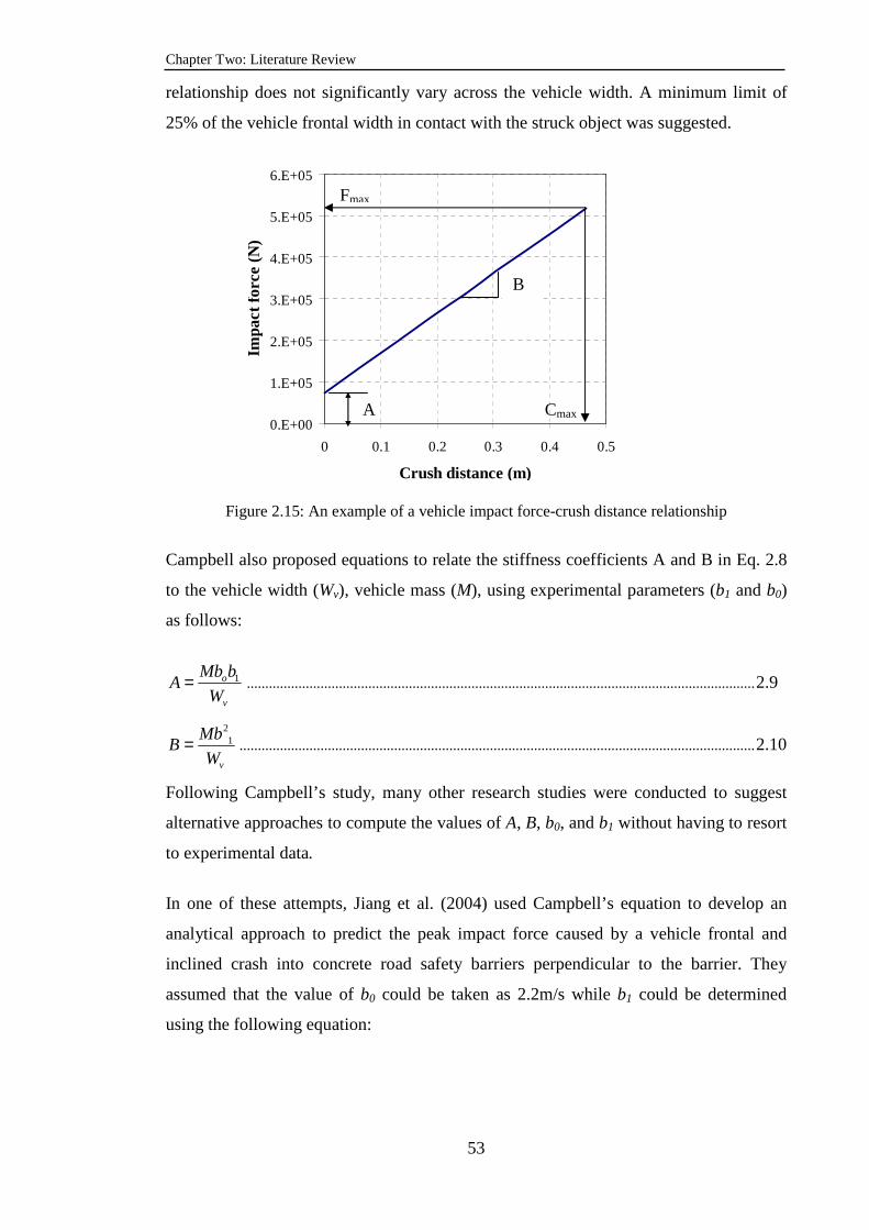
Chapter Two: Literature Review
53
relationship does not significantly vary across the vehicle width. A minimum limit of
25% of the vehicle frontal width in contact with the struck object was suggested.
Figure 2.15: An example of a vehicle impact force-crush distance relationship
Campbell also proposed equations to relate the stiffness coefficients A and B in Eq. 2.8
to the vehicle width (Wv), vehicle mass (M), using experimental parameters (b1 and b0)
as follows:
1o
v
Mb bA
W= .......................................................................................................................................... 2.9
21
v
MbB
W= ............................................................................................................................................ 2.10
Following Campbell’s study, many other research studies were conducted to suggest
alternative approaches to compute the values of A, B, b0, and b1 without having to resort
to experimental data.
In one of these attempts, Jiang et al. (2004) used Campbell’s equation to develop an
analytical approach to predict the peak impact force caused by a vehicle frontal and
inclined crash into concrete road safety barriers perpendicular to the barrier. They
assumed that the value of b0 could be taken as 2.2m/s while b1 could be determined
using the following equation:
0.E+00
1.E+05
2.E+05
3.E+05
4.E+05
5.E+05
6.E+05
0 0.1 0.2 0.3 0.4 0.5
Crush distance (m)
Impa
ct fo
rce
(N)
Cmax
B
A
Fmax
Chapter Two: Literature Review
54
max1 C
bVb o−
=......................................................................................................................................... 2.11
Where: V is the standard vehicle impact velocity used in crash barrier tests (around
56.km/h for most vehicle crash tests).
In their derivations, Jiang et al. (2004) assumed that all the impact energy was absorbed
by vehicle deformation without any contribution from the impacted concrete barrier.
The energy absorbed by vehicle deformation was obtained by integrating equation 2.8
over the damage profile of the vehicle after impact.
On the other hand, Siddall and Day (1996) defined five classes of passenger vehicles
and two classes of pickup, vans and multi-purpose vehicles, and proposed the A and B
values in Table 2.3.
Table 2.3: Generic stiffness coefficients A and B to be used in Campbell’s equation (Siddall and
Day, 1996)
Vehicle type
Passenger vehicles
Pickup Vehicles Van Vehicles Multi-Purpose
Vehicles
Class No.
A (N/m)
B (N/m2)
A (N/m)
B (N/m2)
A (N/m)
B (N/m2)
A (N/m)
B (N/m2)
1 31566 497180 46597 750976 54029 930792 46524 750976 2 32344 457673 38457 471601 62727 1066963 38397 471601 3 36188 482426 n/a n/a n/a n/a n/a n/a 4 37722 459880 n/a n/a n/a n/a n/a n/a 5 50564 782210 n/a n/a n/a n/a n/a n/a
Wågström et al (2004) proposed a stiffness value of 1000kN/m for light vehicles
(1200kg) and medium weight vehicles (1600kg) and 2000 kN/m for heavy vehicles
(2000kg). The proposed values were validated against full frontal rigid barrier crash
tests conducted by the National Highway Traffic Safety Administration (NHTSA) for
different vehicle models, weights and velocities.
In these previous studies, the structure was almost rigid whereas, in the present study,
the structure (column) is flexible and will deform and absorb energy during the impact
process. Nevertheless, this research study will investigate the applicability of the
existing approach. In this study, the method of investigation will include the following
steps:

Chapter Two: Literature Review
55
a) Identifying vehicle characteristics affecting the behaviour of steel columns under
impact;
b) Proposing and validating a simplified vehicle model, based on a comparison of
column behaviour between using a full vehicle model and a simplified vehicle
model. The numerical simulations will be carried out using the finite element
code ABAQUS/Explicit;
c) Suggesting a method to estimate the simplified vehicle characteristics.
2.4. Research methodology and originality Although many research studies have investigated the behaviour of structures under
impact, very few studies have considered axially compressed columns without
longitudinal restraint. Consequently, the practical design of this type of structure is
based on very simple rudimentary rules using an equivalent static load. The aim of this
research is to investigate this problem in detail so as to provide designers with a more
accurate approach. This research will be conducted using numerical simulations to
generate extensive data to guide the development of simplified analytical methods.
Specifically, the objectives of this research are as follows:
1. To suggest and validate a numerical model for the simulation of axially loaded
steel columns subjected to transverse impact using the commercial finite
element code ABAQUS/Explicit. The validation should be based on a
comparison between the proposed simulation model and the relevant
experiments conducted by others;
2. To conduct extensive parametric studies to provide a comprehensive database of
results covering different impact masses, impact velocities and impact locations
in addition to different column boundary conditions, axial load ratios and section
sizes;
3. To develop a simplified numerical vehicle model which can be used to simulate
the effects of vehicle impact on steel columns by using the commercial finite
element code ABAQUS/Explicit;
4. To develop a simplified analytical method for predicting the critical velocity of
rigid body and vehicle impact on the axially compressed steel columns. This
method will be based on the energy balance approach with a quasi-static

Chapter Two: Literature Review
56
approximation of the column behaviour. The numerical simulations’ results will
be used to develop an understanding of the detailed behaviour of steel columns
under transverse impact in order to inform the assumptions of the analytical
method. The numerical simulations’ results will also be used to ascertain the
accuracy of the proposed analytical method;
5. To use the numerical simulations’ results to assess the accuracy of the various
design methods.
2.5. Summary This chapter has presented an overview of the behaviour and the failure modes of
axially loaded columns under transverse impact. The main focus of this chapter has
been to present and discuss the previous research studies in this field so as to identify
gaps in knowledge in order to justify the originality of this research. A further detailed
review of different aspects of this research project will be presented in individual
chapters.
A review of different theoretical developments relating to columns under lateral impact
has been also presented. Clearly, very few of the previous research studies have
addressed the impact behaviour of columns under axial compression and no axial
restraint. The analytical method may be developed based on the energy conservation
principle with a quasi-static approximation of column behaviour. This chapter has
reviewed the basis of this analytical approach and the assumptions and conclusions of
previous related studies. This approach will be fully developed in chapter six.

Chapter Three: Validation of Finite Element Modelling
57
Chapter Three
Validation of Finite Element Modelling Using ABAQUS/Explicit
3.1. Introduction
One of the most effective and accurate numerical methods to handle the problem of
dynamic analysis of structures under impact is the finite element method (Zienkiewicz
and Taylor, 1991, Bonet and Wood, 1997, Crisfield, 1997, Belytschko et al., 2000). For
the problem under consideration in this study, dynamic simulation will be required.
The main objective of this chapter is to validate the application of the general finite
element package ABAQUS/Explicit to the impact problem of this research so that it can
be used to generate extensive numerical results through parametric studies for the
development of a design method. For this, the simulation results will be compared with
relevant experimental and/or numerical results of others available in the literature.
This chapter will present a detailed description of the procedure used in this research
study for modelling axially compressed steel columns subjected to short duration impact
by a rigid mass. This chapter will also describe the geometrical, material, and loading
application parameters used in the numerical model. Special attention will also be paid
to modelling the contact interaction between the impacting body (rigid mass or vehicle)
and the impacted steel column due to its importance to impact analysis. A considerable
sub-section of this chapter will be allocated to describing the material model used in this
study to predict different failure modes of steel under such a transverse impact load.
3.2. Dynamic impact analysis using finite element commercial code
ABAQUS/Explicit
ABAQUS /Explicit is a finite element analysis programme that can be adapted to solve
special cases of transient dynamic problems such as blast and impact by utilizing an
explicit dynamic finite element formulation. In addition to its availability,
ABAQUS/Explicit is considered more appropriate and will be used during this research
project for the following reasons.
Chapter Three: Validation of Finite Element Modelling
58
a) The explicit dynamics method is more suitable to analyzing high-speed and low-
duration dynamic events such as the traverse impact problems investigated in the
present study(SIMULIA, 2010c);
b) Impact load is generated due to the contact interaction between the contacted bodies.
The contact interaction can be formulated more easily in ABAQUS using an
explicit, rather than an implicit dynamics method;
c) In order to predict different failure modes (global and local) that the impacted steel
column may undergo, the analysis procedure along with the material model must be
capable of tracing the response of the column up to failure point. While capturing
local failure occurring in the material usually results in convergence problems in
the implicit analysis procedure, these problems are mitigated considerably in
ABAQUS/Explicit owing to the explicit procedure used in the analysis.
3.2.1. Summary of the explicit dynamics algorithm (SIMULIA, 2010c)
ABAQUS/Explicit does not require solving a system of simultaneous equations as in
the standard finite element procedure. Instead, it integrates the dynamic quantities
(accelerations, velocities, dynamic stresses and strains) over the time increment by
employing an explicit dynamic finite element formulation in which the dynamic
quantities are extracted kinematically from one current time increment to the next one,
as illustrated in Fig. 3.1.

Chapter Three: Validation of Finite Element Modelling
59
Figure 3.1: The computational algorithm used in ABAQUS/Explicit. (Reproduced from (SIMULIA, 2010c) ))
Where:
,y y and y•• •
are the nodal acceleration, velocity and deformation respectively;
M represents the total nodal mass matrix of the system;
I represents the nodal internal forces of the system;
F(t) represents the elements’ externally applied forces at the start of the current time
step (t);
( )tσ represents the element stress at the current time step.
It can be concluded from the above procedure that the values of nodal accelerations,
nodal velocities and nodal displacements at the end of any time increment are merely
based on the same quantities as at the beginning of the current time step, which explains
why this method is considered explicit. Furthermore, it is evident from the previous
Compute stresses,σ , from constitutive equations
based on element strain increments,ε∆ ,
computed from the strain rate,•ε
Integrate the current acceleration
explicitly through the time using central
finite difference method to obtain the
nodal velocity and displacement.
1
( ) ( )( )( ) t tM F Ity••
− = −
Calculate the nodal acceleration at
the beginning of the time step by
applying the dynamic equilibrium
equation.
( )( ) ( , )tt t f σ εσ +∆ ∆=
Set tt ∆+ to t and return to the first step
Element stresses and strains’ calculations.
( ) ( )
( / 2) ( / 2) ( )
(
2t t t
t t t t t
t ty y y
• • ••+∆
+∆ −∆
∆ + ∆= +
)2/()()()( ttttttt ytyy ∆+
•
∆+∆+ ∆+=
Assemble nodal internal forces, )( ttI ∆+ .
Nodal dynamic quantities

Chapter Three: Validation of Finite Element Modelling
60
procedure that, in order to gain accurate results, the time increment must be small
enough to assume the acceleration to be nearly constant throughout that time increment.
3.2.2. Modelling parameters for structural impact simulation using
ABAQUS/Explicit
Simulating the behaviour of structural members under dynamic impact using
ABAQUS/Explicit requires the careful selection of the proper geometrical and material
modelling parameters so as to produce accurate results that are as close as possible to
the actual behaviour of the impacted members. Due to the nature of the problem
investigated in this study which involves applying a static axial force on a steel column
during impact events, a suitable procedure is adopted to apply the axial force using the
quasi-static procedure available in ABAQUS/Explicit. The following sections describe
the modelling approaches and techniques used in the present study:
1. Geometrical modelling;
2. Material modelling;
3. Modelling of the contact between the impacting body and the steel column;
4. Stability limits and time increment control.
5. Damping effect in the impact analysis;
6. Applying the axial force using the quasi-static procedure.
3.2.2.1. Geometrical modelling
Fig. 3.2 shows the main element types used in the present study to simulate the impact
problem which includes solid, shell and spring elements. The differences in these
element types reflect the differences in the geometrical shapes of the structural members
and bodies simulated in the study. These elements belong to the stress/displacement
element library which is the most suitable to model the complex dynamic problems
involving contact, plasticity and large deformations(SIMULIA, 2010b). Linear (first
order) interpolation is used to calculate the internal stresses and strains at any point in
the element which is the only interpolation order offered by ABAQUS/Explicit for solid
and shell elements.

Chapter Three: Validation of Finite Element Modelling
61
Figure 3.2: Linear brick, shell and spring elements used in the present numerical simulation using ABAQUS/Explicit (SIMULIA, 2010b).
Solid elements are used in most of the numerical simulations. Shell elements are used in
simulating hollow steel sections.
For solid and shell elements, ABAQUS/Explicit adopts a reduced integration technique
to integrate various response outputs (stresses and strains) over the element. This
integration technique uses fewer Gaussian integration points than the full integration
scheme. However, the combination of using a reduced integration technique with first
order (linear) interpolation elements leads to what is called the hourglass numerical
problem. To overcome the hourglass problem, ABAQUS/Explicit introduces a small
value of artificial stiffness called “hourglass stiffness” to an element. Moreover, at least
four elements should be used over the thickness of any structural part modelled in order
to obtain accurate results, as shown in Fig. 3.3.
Figure 3.3: Meshing technique used over each thickness of a steel beam using linear elements with reduced integration. Linear elements with reduced integration have also been frequently used by most of the
previous numerical studies to model structural impact problems (Yu and Jones, 1997,
Zeinoddini et al., 2008, Dorogoy and Rittel, 2008, Thilakarathna et al., 2010).
3.2.2.2. Material modelling
When the impacting body impacts the column, a high concentration of stress waves
propagate from the impact point towards the ends of the column in a short period of
Spring element Solid element C3D8R
Shell element S4R
Four elements
Chapter Three: Validation of Finite Element Modelling
62
time (Johnson, 1972, Jones, 1997). This concentration of stresses causes highly
nonlinear local behaviour at the impact zone (Johnson, 1985). With the continuation of
the impact event, a stress wave is generated and spread along the entire column length
causing global deformations and possibly global instability. To account for both local
and global deformations, the adopted material behaviour model must be capable of
tracing the development and propagation of the yielding and inelastic flow of the
material up to the failure point. In addition, the strain rate and the strain hardening
effects are other important issues which must also be simulated properly in the dynamic
impact analysis of strain rate sensitive materials such as steel which is considered in this
study.
For the dynamic analysis of ductile members, ABAQUS/Explicit provides two material
models to account for the inelastic behaviour and the local failure of the structural
members under dynamic loads. These are the classical metal plasticity model and the
progressive damage and failure model. The two models work in conjunction with each
other to trace the full response of the material up to failure. These models can consider
the effects of strain hardening, strain rate sensitivity and material failure. The following
two sections will describe in detail the important characteristics of each model.
A. Classical metal plasticity model (SIMULIA, 2010a)
This model uses von Mises or Hill yield stress with the corresponding plastic flow to
simulate both isotropic and anisotropic yielding of the material. The model uses the true
stress-true strain curve of the material to describe the inelastic response and defines the
elastic response in terms of the material modulus of elasticity, see Fig. 3.4. The strain
hardening and the strain rate effects can be accounted for in this material model with an
acceptable accuracy especially for low strain rates. Hence, it can be adopted for the
vehicle impact problem investigated in the present study. In addition, the classical metal
model can be used in conjunction with the progressive damage and failure model
available in ABAQUS/Explicit to simulate shear and tensile failures. Both failure
modes can occur in transversely impacted steel members (Menkes and Opat, 1973, Yu
and Jones, 1991, Yu and Jones, 1997).
B. Strain hardening
Strain hardening plays a significant role in the nonlinear response of structural metals
such as steel under dynamic impact loads. It has been shown by Bai and Pedersen
Chapter Three: Validation of Finite Element Modelling
63
(1993) that when strain hardening is included in the material behaviour of a structural
member subjected to transverse impact, the structure becomes stiffer, resulting in a
smaller strain energy absorption. In this study, the strain hardening behaviour of the
steel is modelled using isotropic strain hardening in which the increase in yield stress is
assumed to be equal in all directions with the increasing plastic strain. The strain
hardening behaviour is defined in ABAQUS/Explicit as the yield stress-plastic strain
relationship. Fig. 3.4 shows the effect of strain hardening on the typical stress-plastic
strain behaviour of steel.
Figure 3.4: Typical true plastic stress-true plastic strain relationship of steel, including strain hardening and strain rate effects.
C. Strain rate dependence
Strain-rate dependence or strain-rate sensitivity is one of the most important material
dynamic phenomena that must be included in the impact analysis of structures. For
strain-rate sensitive material such as steel or aluminium, the yield stress increases
considerably due to the rapid increase in strain, see Fig. 3.4. This increase in yield stress
depends on the material type and the rate of strain increase (Cowper and Symonds,
1957).
Two methods are offered by ABAQUS/Explicit to introduce the effects of strain-rate-
dependence in the material model. These are using the Cowper-Symonds over-stress
power law and using the tubular input of yield ratios. The Cowper-Symonds equation is
used in this research. It has been used by many numerical studies to simulate the strain
rate dependence of steel subjected to impact loads (Yu and Jones, 1997, Zeinoddini et
al., 2008, Thilakarathna et al., 2010, Bambach, 2011).
0.0E+00
2.0E+08
4.0E+08
6.0E+08
8.0E+08
1.0E+09
1.2E+09
1.4E+09
0.0 0.2 0.4 0.5 0.7Plastic strain
Mis
es s
tres
s (N
/m2
)
Without strain rate effect
With strain rate effect
Strain rate effect
Strain hardening effect
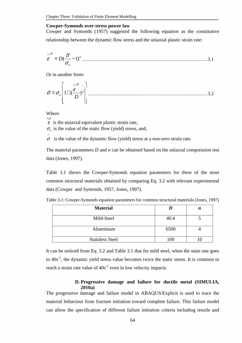
Chapter Three: Validation of Finite Element Modelling
64
Cowper-Symonds over-stress power law Cowper and Symonds (1957) suggested the following equation as the constitutive
relationship between the dynamic flow stress and the uniaxial plastic strain rate:
( 1)pl
n
o
Dσεσ
•= − .......................................................................................................................... 3.1
Or in another form:
1
1 ( )
pl
no D
εσ σ•
= +
.................................................................................................................... 3.2
Where
pl•
ε is the uniaxial equivalent plastic strain rate,
oσ is the value of the static flow (yield) stress, and, −
σ is the value of the dynamic flow (yield) stress at a non-zero strain rate. The material parameters D and n can be obtained based on the uniaxial compression test
data (Jones, 1997).
Table 3.1 shows the Cowper-Symonds equation parameters for three of the most
common structural materials obtained by comparing Eq. 3.2 with relevant experimental
data (Cowper and Symonds, 1957, Jones, 1997).
Table 3.1: Cowper-Symonds equation parameters for common structural materials (Jones, 1997)
Material D n
Mild-Steel 40.4 5
Aluminium 6500 4
Stainless Steel 100 10 It can be noticed from Eq. 3.2 and Table 3.1 that for mild steel, when the stain rate goes
to 40s-1, the dynamic yield stress value becomes twice the static stress. It is common to
reach a strain rate value of 40s-1 even in low velocity impacts.
D. Progressive damage and failure for ductile metal (SIMULIA,
2010a) The progressive damage and failure model in ABAQUS/Explicit is used to trace the
material behaviour from fracture initiation toward complete failure. This failure model
can allow the specification of different failure initiation criteria including tensile and

Chapter Three: Validation of Finite Element Modelling
65
shear failure. In this failure model, the material stiffness is degraded progressively after
damage initiation according to a specified damage evolution response. This progressive
damage allows for a smooth degradation of the material stiffness, making it suitable for
both quasi-static and dynamic situations. The model offers two choices after complete
failure, these being the removal of elements from the mesh and keeping it in the model
but with a zero stress value.
The progressive damage and failure model provided in ABAQUS/Explicit is employed
in the present numerical model in conjunction with the isotropic metal plasticity model.
According to this model, the typical stress–strain behaviour of steel with strain
hardening and strain rate effects undergoing tensile or shear failure is shown in Fig. 3.5
(SIMULIA, 2010a).
Figure 3.5: Typical uniaxial stress-strain response of the steel with progressive damage evolution up to failure. Fig. 3.5 shows a typical stress-strain curve for a progressive damage and failure model
for a ductile material. It consists of three parts: the undamaged material behaviour (a-b-
c-d′ in Fig 3.5), the damage initiation criterion (point c in Fig 3.5), and the damage
evolution law (c-d in Fig 3.5). The first part represents the material stress-strain
response in the absence of damage which can be obtained from uniaxial tensile test
while the following sub-sections describe the approach used in the present study to
define the other two parts which deal with damage.
0.0E+00
4.5E+08
9.0E+08
1.4E+09
1.8E+09
0.0 0.2 0.4 0.6 0.8 1.0 1.2
Strain
Str
ess (
N/m
2 )
`
1d• =
b
c
d a
•
•
0d• =
•
ploε
E
E
yoσ
oσ
plfε
•
d′
Chapter Three: Validation of Finite Element Modelling
66
Part 2. Damage initiation criterion The damage initiation criterion represents the point in the material true stress-true strain
response where damage starts to develop and progress. For metals, two damage
initiation criteria are offered by ABAQUS/Explicit according to the fracture
mechanism. Both of these criteria are employed in the present study. They are:
1. The ductile damage criterion (for tensile fracture)
The ductile damage criterion uses the equivalent plastic strain limit at the onset of
damage pl
Dε as the failure initiation criterion. The value of this strain is described as a
function of plastic strain rate pl
ε•
and stress triaxiality η as follows:
( , )pl pl
Dε η ε•
..................................................................................................................................... 3.3
Where the stress triaxiality η is defined by ABAQUS as the ratio of the pressure stress
to the equivalent Mises stress ( p
qη −= ).
Material degradation is assumed to start when the damage initiation criterion fΦ is met
based on the following condition:
1=∆
=Φ ∑pl
D
pl
f
ε
ε
........................................................................................................................... 3.4
Where ∑∆pl
ε is the accumulative value of the equivalent plastic strain.
Implementing the above damage criterion is undertaken in two steps in this study. In the
first step, a nonlinear dynamic analysis is performed using ABAQUS/Explicit under the
same loading condition but using the isotropic metal plasticity constitutive model to
obtain the values of the maximum stress triaxiality and strain rate corresponding to the
loading condition for the entire model. Then, the fracture strain is obtained from the true
stress versus the true strain curve extracted from the uniaxial tensile test of the material.
In the second step, the values of fracture strain together with the values of strain rate
and stress triaxiality are used as input data in the material damage model.
Chapter Three: Validation of Finite Element Modelling
67
2. Shear damage initiation criterion.
Here, the damage initiation criterion is described in terms of the equivalent plastic strain
at the onset of shear damage (pl
Sε ). The value of this strain is a function of the strain
rate pl
ε•
and the shear stress ratio Sθ (Boh et al., 2004, SIMULIA, 2010a).
( , )pl pl
s Sε θ ε•
.................................................................................................................................... 3.5
Where shear stress ratio Sθ is defined as:
max
( )sS
q k pθτ+= ................................................................................................................................... 3.6
Where maxτ is the maximum shear stress and ks is a material parameter.
Material degradation starts when the damage initiation criterion SΦ is met based on the
following condition:
1
pl
S pl
S
ε
ε
∆Φ = =∑
............................................................................................................................ 3.7
Where ∑∆pl
ε is the accumulative value of the equivalent plastic strain.
The same procedure that is used to implement the ductile damage criterion is used to
implement the shear damage criterion, except that the maximum shear stress ratio is
extracted from the first step of the nonlinear dynamic analysis.
Part 3. Damage evolution and degradation Once damage initiation is detected at any element using any of the aforementioned
damage initiation criteria, the damage process starts and continues to cause progressive
degradation of the material stiffness of the element until failure. The rate of degradation
with time is referred to as the damage evolution law which can be specified either as
effective plastic displacement or fracture energy dissipation(SIMULIA, 2010a). In this
study, the damage evolution law in all numerical simulations uses an effective plastic
displacement assuming a linear relationship between the damage variable (d) and the
effective plastic displacement plu (Qiao et al., 2006). The damage variable represents
the accumulated ratio of the effective plastic displacement plu to the total plastic
displacement at the point of failure (full degradation), plfu , as shown in the following
equation:
Chapter Three: Validation of Finite Element Modelling
68
plf
pl
u
ud
••= .......................................................................................................................................... 3.8
The effective plastic displacement plu is defined with the following evolution
equations:
pl plcu L ε• •= .................................................................................................................................... 3.9
pl pl
f c fu L ε= .................................................................................................................................... 3.10
Where Lc is the characteristic length of the element defined as the square root of the
integration point area for shell elements and the cubic root of the integration point
volume for solid elements(SIMULIA, 2010a); plfε is taken as the strain at the complete
failure of the material taken from the uniaxial stress strain curve.
Using the effective plastic displacement approach as the damage evolution law helps to
reduce the mesh dependency of the results. By using this approach, the degradation
response of the material is characterized by a stress-displacement behaviour rather than
a stress-strain behaviour. According to the definition of the damage variable •d , its
value ranges from 0 corresponding to damage initiation to 1 representing complete
failure. For solid element, failure is assumed to take place when (•d =1) at any one
integration point of an element in the model. However, in a shell element all through the
thickness section points at any one integration location of an element must fail before
the element failure. In any case, when complete failure occurs, ABAQUS/Explicit offers
two procedures to complete the analysis: either by removing the failed element from the
model mesh or by keeping it but setting its stress to zero in the next analysis step. The
first option is used in the present study.
In this research study, the material model combining classical metal plasticity with
progressive damage and failure is used because it is the most general, effective and easy
one to use.
3.2.2.3. Modelling of contact (SIMULIA, 2010d)
When two bodies impact on each other, a contact interaction develops between the
contacted surfaces at the impact zone. This interaction generates a concentrated stress
and/or pressure at each surface with a value depending on the geometrical, material and
dynamic characteristics of each body at the time of impact in addition to the mechanical
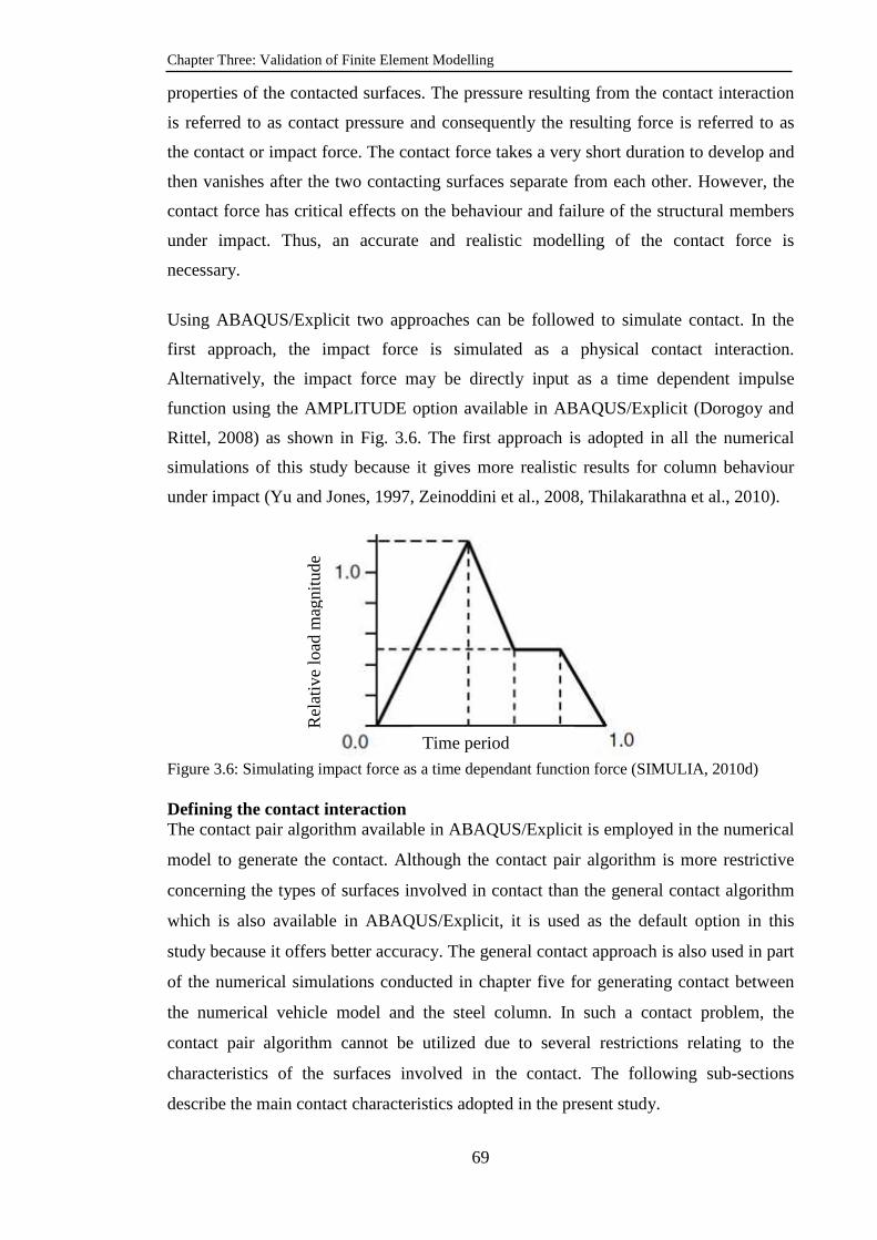
Chapter Three: Validation of Finite Element Modelling
69
properties of the contacted surfaces. The pressure resulting from the contact interaction
is referred to as contact pressure and consequently the resulting force is referred to as
the contact or impact force. The contact force takes a very short duration to develop and
then vanishes after the two contacting surfaces separate from each other. However, the
contact force has critical effects on the behaviour and failure of the structural members
under impact. Thus, an accurate and realistic modelling of the contact force is
necessary.
Using ABAQUS/Explicit two approaches can be followed to simulate contact. In the
first approach, the impact force is simulated as a physical contact interaction.
Alternatively, the impact force may be directly input as a time dependent impulse
function using the AMPLITUDE option available in ABAQUS/Explicit (Dorogoy and
Rittel, 2008) as shown in Fig. 3.6. The first approach is adopted in all the numerical
simulations of this study because it gives more realistic results for column behaviour
under impact (Yu and Jones, 1997, Zeinoddini et al., 2008, Thilakarathna et al., 2010).
Figure 3.6: Simulating impact force as a time dependant function force (SIMULIA, 2010d) Defining the contact interaction The contact pair algorithm available in ABAQUS/Explicit is employed in the numerical
model to generate the contact. Although the contact pair algorithm is more restrictive
concerning the types of surfaces involved in contact than the general contact algorithm
which is also available in ABAQUS/Explicit, it is used as the default option in this
study because it offers better accuracy. The general contact approach is also used in part
of the numerical simulations conducted in chapter five for generating contact between
the numerical vehicle model and the steel column. In such a contact problem, the
contact pair algorithm cannot be utilized due to several restrictions relating to the
characteristics of the surfaces involved in the contact. The following sub-sections
describe the main contact characteristics adopted in the present study.
Rel
ativ
e lo
ad m
agni
tude
Time period
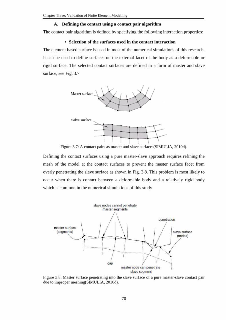
Chapter Three: Validation of Finite Element Modelling
70
A. Defining the contact using a contact pair algorithm
The contact pair algorithm is defined by specifying the following interaction properties:
• Selection of the surfaces used in the contact interaction
The element based surface is used in most of the numerical simulations of this research.
It can be used to define surfaces on the external facet of the body as a deformable or
rigid surface. The selected contact surfaces are defined in a form of master and slave
surface, see Fig. 3.7
Figure 3.7: A contact pairs as master and slave surfaces(SIMULIA, 2010d).
Defining the contact surfaces using a pure master-slave approach requires refining the
mesh of the model at the contact surfaces to prevent the master surface facet from
overly penetrating the slave surface as shown in Fig. 3.8. This problem is most likely to
occur when there is contact between a deformable body and a relatively rigid body
which is common in the numerical simulations of this study.
Figure 3.8: Master surface penetrating into the slave surface of a pure master-slave contact pair due to improper meshing(SIMULIA, 2010d).
Master surface
Salve surface
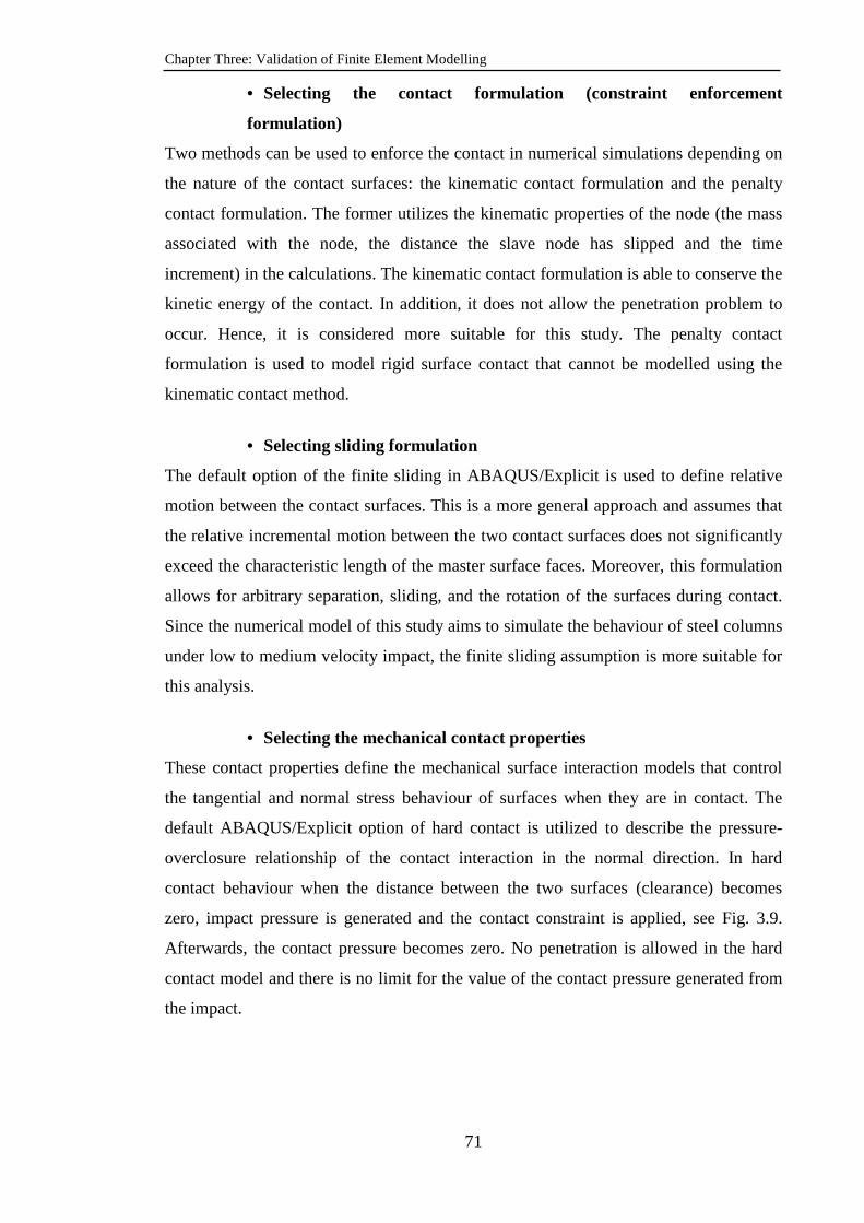
Chapter Three: Validation of Finite Element Modelling
71
• Selecting the contact formulation (constraint enforcement
formulation)
Two methods can be used to enforce the contact in numerical simulations depending on
the nature of the contact surfaces: the kinematic contact formulation and the penalty
contact formulation. The former utilizes the kinematic properties of the node (the mass
associated with the node, the distance the slave node has slipped and the time
increment) in the calculations. The kinematic contact formulation is able to conserve the
kinetic energy of the contact. In addition, it does not allow the penetration problem to
occur. Hence, it is considered more suitable for this study. The penalty contact
formulation is used to model rigid surface contact that cannot be modelled using the
kinematic contact method.
• Selecting sliding formulation
The default option of the finite sliding in ABAQUS/Explicit is used to define relative
motion between the contact surfaces. This is a more general approach and assumes that
the relative incremental motion between the two contact surfaces does not significantly
exceed the characteristic length of the master surface faces. Moreover, this formulation
allows for arbitrary separation, sliding, and the rotation of the surfaces during contact.
Since the numerical model of this study aims to simulate the behaviour of steel columns
under low to medium velocity impact, the finite sliding assumption is more suitable for
this analysis.
• Selecting the mechanical contact properties
These contact properties define the mechanical surface interaction models that control
the tangential and normal stress behaviour of surfaces when they are in contact. The
default ABAQUS/Explicit option of hard contact is utilized to describe the pressure-
overclosure relationship of the contact interaction in the normal direction. In hard
contact behaviour when the distance between the two surfaces (clearance) becomes
zero, impact pressure is generated and the contact constraint is applied, see Fig. 3.9.
Afterwards, the contact pressure becomes zero. No penetration is allowed in the hard
contact model and there is no limit for the value of the contact pressure generated from
the impact.

Chapter Three: Validation of Finite Element Modelling
72
Figure 3.9: Contact pressure-clearance relationship for hard contact (SIMULIA, 2010d)
For the tangential direction, ABAQUS/Explicit offers more than one model to describe
the friction formulation. The isotropic penalty friction formulation is used throughout
this study. This model uses the Coulomb friction model to relate the maximum
allowable frictional stress to the contact pressure. The model allows for the specifying
of the coefficient between the contact surfaces and assumes that the coefficient is the
same in all directions. Frictionless and rough friction models are also available in
ABAQUS/Explicit and they can be used to simulate the non-friction and nonslip
behaviour of contact respectively. Nevertheless, because of the very short duration of
the impact event, the effect of friction behaviour on contact interaction is very low.
Other characteristics of contact, such as the tracking approach and contact weighing
algorithm, are chosen automatically by ABAQUS/Explicit.
B. Defining the contact using the general contact approach ABQUS/Explicit has several requirements on the surfaces involved in the contact
problem in order to be able to use the contact pair algorithm. Some of these restrictions
are not satisfied in the full scale numerical vehicle model, used in chapter five, such as
the fact that the contact surfaces are not continuous and deformable and rigid bodies are
combined to define a single surface at some of the contact surfaces. This is because the
vehicle model comprises different components modelled using deformable bodies, rigid
bodies and rigid surfaces with different element types. This variety in the element types,
in addition to the nature of the geometrical shape of the vehicle, restricts the use of the
contact pair algorithm. Therefore, general contact approach is used in the numerical
simulations performed in chapter five to simulate the contact because it allows simple
definitions of contact with very few restrictions on the types of surfaces involved.
Chapter Three: Validation of Finite Element Modelling
73
The same modelling parameters used to define the contact pair algorithm are used to
define the general contact in ABAQUS/Explicit, except that the general contact
algorithm uses only the penalty enforcement method to enforce contact constraints
between the contacting surfaces.
3.2.2.4. Stability limit and time increment control
The stability limit in ABAQUS/Explicit can be defined as the maximum time increment
that can be used in the dynamic explicit analysis procedure(SIMULIA, 2010c). The
highly geometrical and material nonlinearities of the dynamic impact problem of this
research require the stability limit of the model to be changed continuously. Therefore,
the full automatic time increment is used in all numerical simulations in this study to
automatically adjust the time increment. In this time increment strategy, the analysis
starts by calculating the stability limit based on the maximum frequency of all the
individual elements in the system using the element by element search method as in the
following:
d
estable c
Lt =∆ .................................................................................................................................... 3.11
Where:
eL is the element length taken as the shortest element distance, and
dc is the material wave speed calculated from the equation:
ρE
cd = .......................................................................................................................................... 3.12
Where E is the modulus of elasticity of the material, and ρ is the material density. Afterwards and according to the nature of the problem under investigation, the stability
limit may be defined in terms of the maximum frequency of the dynamic system which
is referred to as the global stability limit using the following equation:
( )2max max
max
21stablet ξ ξ
ω∆ = + − ............................................................................................... 3.13
Where maxω is the maximum frequency of the dynamic system and ξmax is the
corresponding damping ratio defined by:

Chapter Three: Validation of Finite Element Modelling
74
c
c
cξ = .............................................................................................................................................. 3.14
Where c is the damping constant of the system and cc is the critical damping value
described by:
cc =2MT maxω .................................................................................................................................. 3.15
Where MT is the total mass of the structural system.
For an un-damped system ξ =0 which is often used in impact simulations. Then the
stability limit according to Eq. 3.13 becomes:
max
2
ω=∆ stablet ................................................................................................................................ 3.16
The full automatic increment control is more conservative, especially during the initial
part of the analysis when using the element by element basis to estimate the stability
limit. It also has more control on the progress of the analysis. Therefore, it is adopted in
this study.
3.2.2.5. Damping effects
Damping has no significant effect on structural behaviour for the simulated cases in this
study because the duration of the impact is very short compared to the natural period of
the structure system (Jones, 1997, Sastranegara et al., 2006, Zeinoddini et al., 2008,
Thilakarathna et al., 2010). However, to investigate any possible effect of damping, the
procedure below is used to determinate the damping coefficient.
In ABAQUS/Explicit the damping effect can be accounted for in the material modelling
phase by employing the Rayleigh damping procedure(SIMULIA, 2010a). Rayleigh
damping assumes that the damping matrix is a linear combination of mass and stiffness
matrices, as follows (Clough and Penzien, 1975, Humar, 2002):
C M Kα β = + ................................................................................................................. 3.17
Where:
M and K
are the nodal mass and stiffness matrices of the structural system,
C is the damping matrix of the structure, and
α and β are the mass and stiffness proportional Rayleigh damping factors respectively.
Chapter Three: Validation of Finite Element Modelling
75
For a given mode of vibration m, the Rayleigh damping factors (α and β ) can be
related to each other using the following expression:
2 2m
mm
β ωαξω
×= + ....................................................................................................................... 3.18
Where mω is the frequency of the vibration mode m and ξm is the damping ratio
specified for the vibration mode m
Eq. 3.18 indicates that the mass proportional Rayleigh damping, α , affects damping of
the lower frequency modes while the stiffness proportional Rayleigh damping, β ,
affects damping of the higher frequency mode (SIMULIA, 2010a). Moreover, Eq. 3.18
shows that, for the maximum frequency mode of the structure, maxω , the value of maxξ
increases when the stiffness proportional Rayleigh damping, β increases as in the
following equation.
maxmax
max2 2
β ωαξω
×= + ............................................................................................. 3.19
On the other hand, Eq. 3.13 shows that the time increment for numerical stability in
ABAQUS/Explicit decreases with increasing maxξ . Therefore, using the stiffness
proportional Rayleigh damping, β , to damp out the lowest frequency mode in
ABAQUS/Explicit significantly decreases time increment for stable dynamic analysis.
Hence, using the mass proportional damping, α , is more suitable to damp out the low
frequency response in ABAQUS/Explicit analysis (Thilakarathna et al., 2010,
SIMULIA, 2010a).
For low frequency response, the mass proportional damping, α , can be calculated by
neglecting the contribution of the stiffness proportional damping (i.e. β =0), in Eq.
3.18, to obtain the following equation:
2 m mα ω ξ= ....................................................................................................................................... 3.20
The natural frequency of the structural dynamic system, mω , can be calculated in the
linear perturbation analysis available in ABAQUS/Standard while the damping ratio

Chapter Three: Validation of Finite Element Modelling
76
needs to be assumed in advance according to the nature of the structural system. Once
the damping ratio is assumed and the frequency is determined, the Rayleigh mass
proportional damping factor can be subsequently calculated from Eq. 3.20. Section 3.3
gives an example of the effects of damping.
3.2.2.6. Sequence of axial load application
The numerical model developed in this study is mainly intended to simulate the
behaviour and failure modes of an impacted steel column under a static compressive
axial load. Therefore, the model must be able to maintain a static axial load on the
structural member while the member is subjected to dynamic impact. This means that
both the static and dynamic loads should be exerted simultaneously during the entire
dynamic analysis duration. In ABAQUS/Explicit, only one dynamic analysis is allowed.
Therefore, the only way to simulate the static load effect is to apply the axial load as a
quasi-static load using the quasi-static analysis procedure available in
ABAQUS/Explicit (SIMULIA, 2010e). To perform a quasi-static analysis, the load
should be applied as a time dependant function using the SMOOTH AMPLITUDE
option(SIMULIA, 2010d), see Fig. 3.10. Furthermore, the time period during which the
load is applied must not be less than the natural period of the structural system to
produce accurate static results by eliminating pseudo-dynamic effects (SIMULIA,
2010e, Biggs, 1964).
Figure 3.10: Smooth step amplitude curve used to define a quasi-static load (SIMULIA, 2010e) To ensure that the load effect is static rather than dynamic, the kinetic energy of the
deformable structural system should not exceed 10% of the total strain
energy(SIMULIA, 2010e), see Fig. 3.11.
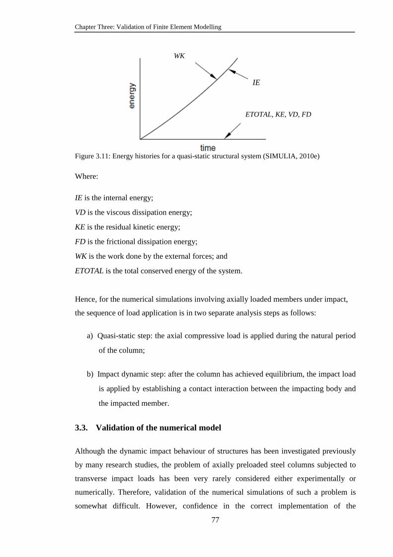
Chapter Three: Validation of Finite Element Modelling
77
Figure 3.11: Energy histories for a quasi-static structural system (SIMULIA, 2010e)
Where:
IE is the internal energy;
VD is the viscous dissipation energy;
KE is the residual kinetic energy;
FD is the frictional dissipation energy;
WK is the work done by the external forces; and
ETOTAL is the total conserved energy of the system.
Hence, for the numerical simulations involving axially loaded members under impact,
the sequence of load application is in two separate analysis steps as follows:
a) Quasi-static step: the axial compressive load is applied during the natural period
of the column;
b) Impact dynamic step: after the column has achieved equilibrium, the impact load
is applied by establishing a contact interaction between the impacting body and
the impacted member.
3.3. Validation of the numerical model
Although the dynamic impact behaviour of structures has been investigated previously
by many research studies, the problem of axially preloaded steel columns subjected to
transverse impact loads has been very rarely considered either experimentally or
numerically. Therefore, validation of the numerical simulations of such a problem is
somewhat difficult. However, confidence in the correct implementation of the
ETOTAL, KE, VD, FD
WK
IE

Chapter Three: Validation of Finite Element Modelling
78
simulation procedure can be developed through a simulation of the general dynamic
transverse impact problem by checking the modelling approaches used in this study as
described in the previous sections.
In this section, the ABAQUS/Explicit simulation results will be assessed against three
series of published experimental tests. These three series of experiments are selected to
ensure that different possible column failure modes are covered. These validation test
series are:
Transverse impact tests on steel tubes under an axial compressive load
(Zeinoddini et al., 2002, Zeinoddini et al., 2008);
Transverse impact tests of clamped steel beams with a rectangular hollow
section (Bambach et al., 2008); and
Transverse impact tests of rectangular clamped steel beams (Yu and Jones,
1991, Yu and Jones, 1997).
3.3.1. Global plastic buckling failure
Tests were conducted by Zeinoddini et al.(2002). In these tests, the steel tube was one
metre long; it was pre-compressed and then impacted at the midpoint using a drop
weight of 25.45 kg with a falling velocity of about 7 m/s (about 25 km/hour). The
testing rig of the experiment was set up to provide fixed support at one end of each
specimen and sliding support at the other. The tubes were loaded to different levels of
axial compression loads. The test set up is shown in Fig. 3.12 together with the present
ABAQUS model.
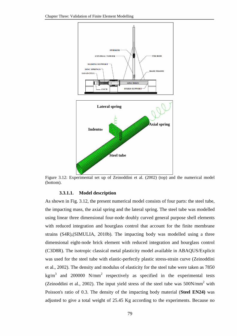
Chapter Three: Validation of Finite Element Modelling
79
Figure 3.12: Experimental set up of Zeinoddini et al. (2002) (top) and the numerical model (bottom).
3.3.1.1. Model description
As shown in Fig. 3.12, the present numerical model consists of four parts: the steel tube,
the impacting mass, the axial spring and the lateral spring. The steel tube was modelled
using linear three dimensional four-node doubly curved general purpose shell elements
with reduced integration and hourglass control that account for the finite membrane
strains (S4R),(SIMULIA, 2010b). The impacting body was modelled using a three
dimensional eight-node brick element with reduced integration and hourglass control
(C3D8R). The isotropic classical metal plasticity model available in ABAQUS/Explicit
was used for the steel tube with elastic-perfectly plastic stress-strain curve (Zeinoddini
et al., 2002). The density and modulus of elasticity for the steel tube were taken as 7850
kg/m3 and 200000 N/mm2 respectively as specified in the experimental tests
(Zeinoddini et al., 2002). The input yield stress of the steel tube was 500N/mm2 with
Poisson's ratio of 0.3. The density of the impacting body material (Steel EN24) was
adjusted to give a total weight of 25.45 Kg according to the experiments. Because no
Axial spring Indentor
Lateral spring
Steel tube
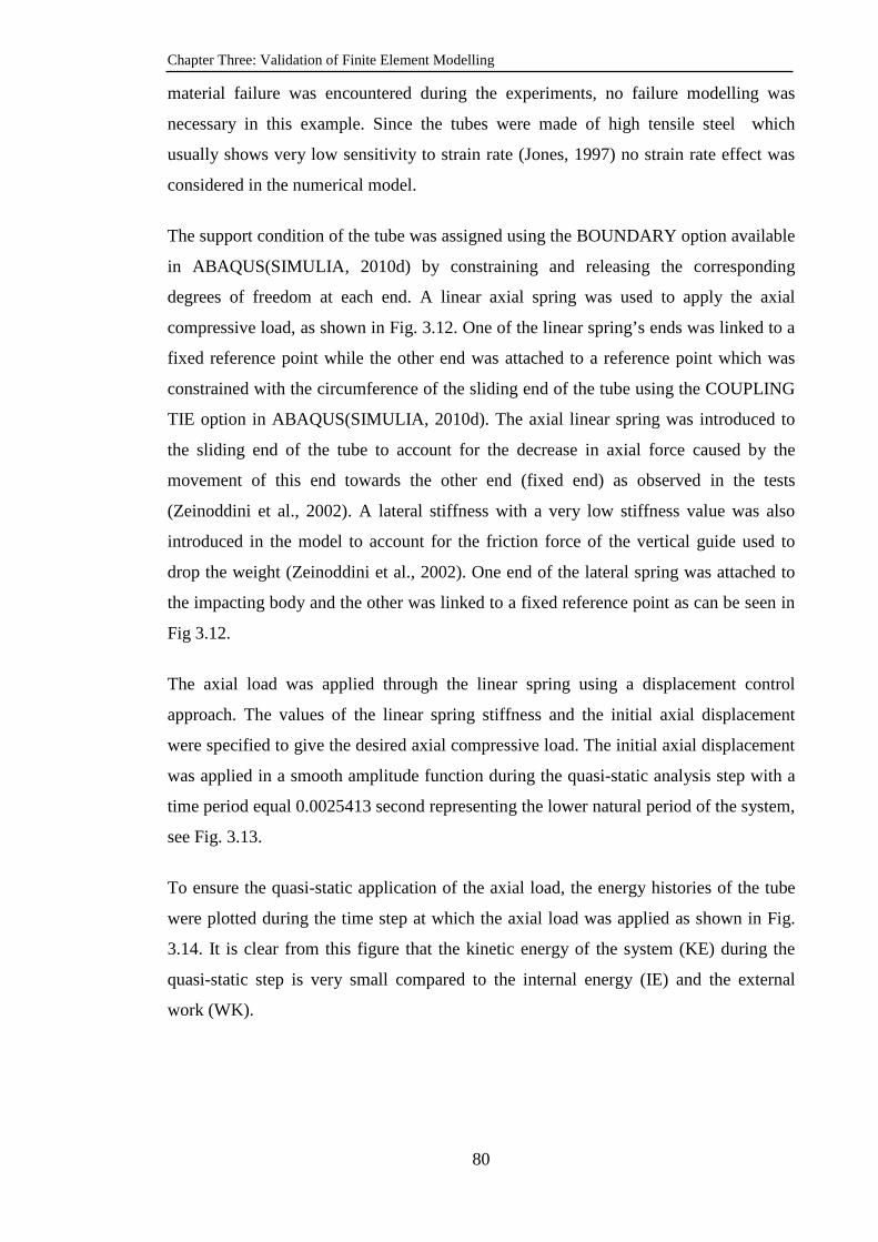
Chapter Three: Validation of Finite Element Modelling
80
material failure was encountered during the experiments, no failure modelling was
necessary in this example. Since the tubes were made of high tensile steel which
usually shows very low sensitivity to strain rate (Jones, 1997) no strain rate effect was
considered in the numerical model.
The support condition of the tube was assigned using the BOUNDARY option available
in ABAQUS(SIMULIA, 2010d) by constraining and releasing the corresponding
degrees of freedom at each end. A linear axial spring was used to apply the axial
compressive load, as shown in Fig. 3.12. One of the linear spring’s ends was linked to a
fixed reference point while the other end was attached to a reference point which was
constrained with the circumference of the sliding end of the tube using the COUPLING
TIE option in ABAQUS(SIMULIA, 2010d). The axial linear spring was introduced to
the sliding end of the tube to account for the decrease in axial force caused by the
movement of this end towards the other end (fixed end) as observed in the tests
(Zeinoddini et al., 2002). A lateral stiffness with a very low stiffness value was also
introduced in the model to account for the friction force of the vertical guide used to
drop the weight (Zeinoddini et al., 2002). One end of the lateral spring was attached to
the impacting body and the other was linked to a fixed reference point as can be seen in
Fig 3.12.
The axial load was applied through the linear spring using a displacement control
approach. The values of the linear spring stiffness and the initial axial displacement
were specified to give the desired axial compressive load. The initial axial displacement
was applied in a smooth amplitude function during the quasi-static analysis step with a
time period equal 0.0025413 second representing the lower natural period of the system,
see Fig. 3.13.
To ensure the quasi-static application of the axial load, the energy histories of the tube
were plotted during the time step at which the axial load was applied as shown in Fig.
3.14. It is clear from this figure that the kinetic energy of the system (KE) during the
quasi-static step is very small compared to the internal energy (IE) and the external
work (WK).
Chapter Three: Validation of Finite Element Modelling
81
0.0E+00
4.0E+04
8.0E+04
1.2E+05
1.6E+05
2.0E+05
0.0000 0.0005 0.0010 0.0016 0.0021 0.0026
Time (Sec.)
Axi
al l
oad
(N)
(P/Py)=0.5
(P/Py)=0.6
(P/Py)=0.7
Figure 3.13: Smooth amplitude functions used to apply the quasi-static load
Figure 3.14: Energy histories during the quasi-static load application, (P/Py) =0.5.
The contact pair algorithm available in ABAQUS/Explicit was used to simulate the
contact interaction between the impacting mass and the steel tube. Hard contact and
penalty friction formulation were used to describe normal and tangential behaviours
respectively as mechanical interaction properties with the coefficient of fiction was
assumed to be 0.47. Kinematic contact enforcement method was adopted to detect
contact between the two bodies with small sliding formulation.
3.3.1.2. Simulation results
The experimental results indicated global column failure in the columns with an axial
load value above 65% of the tube squash load (Zeinoddini et al., 2002). In this failure
mode, the column lost its stability and large lateral deformations developed causing the
column to shorten and slide towards the fixed end. For lower axial load ratios, no global
failure occurred but local and plastic deformations and indentations were recorded at the
impact zone (Zeinoddini et al., 2002, Zeinoddini et al., 2008). In the present numerical
0.E+00
2.E+03
4.E+03
6.E+03
8.E+03
1.E+04
0.0000 0.0005 0.0010 0.0016 0.0021 0.0026
Time (Sec.)
Ene
rgy
(Jou
le)
WK
IE
ETOTAL, KE, VD, FD
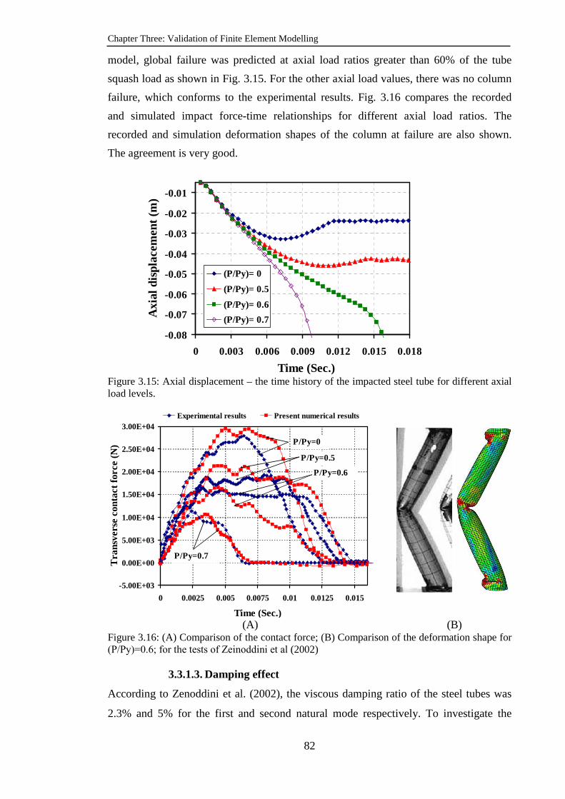
Chapter Three: Validation of Finite Element Modelling
82
model, global failure was predicted at axial load ratios greater than 60% of the tube
squash load as shown in Fig. 3.15. For the other axial load values, there was no column
failure, which conforms to the experimental results. Fig. 3.16 compares the recorded
and simulated impact force-time relationships for different axial load ratios. The
recorded and simulation deformation shapes of the column at failure are also shown.
The agreement is very good.
-0.08
-0.07
-0.06
-0.05
-0.04
-0.03
-0.02
-0.01
0 0.003 0.006 0.009 0.012 0.0150.018
Time (Sec.)
Axi
al d
ispl
acem
ent (
m)
(P/Py)= 0
(P/Py)= 0.5
(P/Py)= 0.6
(P/Py)= 0.7
Figure 3.15: Axial displacement – the time history of the impacted steel tube for different axial load levels.
(A) (B)
Figure 3.16: (A) Comparison of the contact force; (B) Comparison of the deformation shape for (P/Py)=0.6; for the tests of Zeinoddini et al (2002)
3.3.1.3. Damping effect
According to Zenoddini et al. (2002), the viscous damping ratio of the steel tubes was
2.3% and 5% for the first and second natural mode respectively. To investigate the
-5.00E+03
0.00E+00
5.00E+03
1.00E+04
1.50E+04
2.00E+04
2.50E+04
3.00E+04
0 0.0025 0.005 0.0075 0.01 0.0125 0.015
Time (Sec.)
Tra
nsve
rse
cont
act f
orce
(N
)
Experimental results Present numerical results
P/Py=0
P/Py=0.5
P/Py=0.6
P/Py=0.7
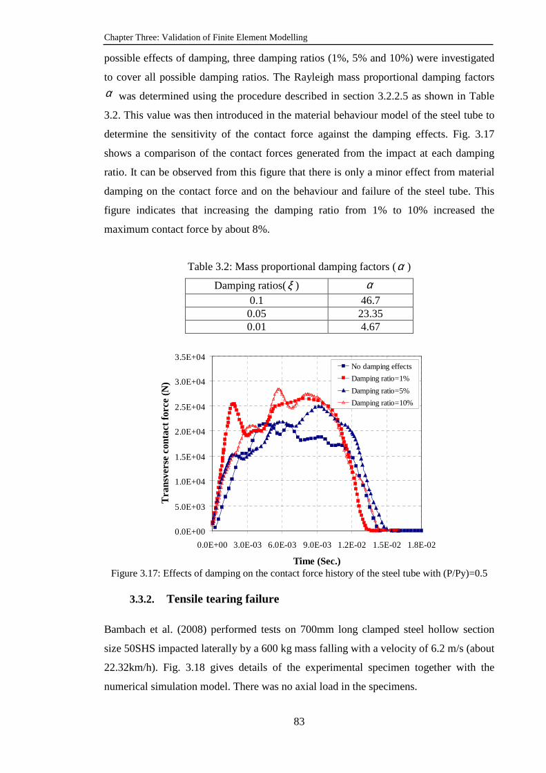
Chapter Three: Validation of Finite Element Modelling
83
possible effects of damping, three damping ratios (1%, 5% and 10%) were investigated
to cover all possible damping ratios. The Rayleigh mass proportional damping factors
α was determined using the procedure described in section 3.2.2.5 as shown in Table
3.2. This value was then introduced in the material behaviour model of the steel tube to
determine the sensitivity of the contact force against the damping effects. Fig. 3.17
shows a comparison of the contact forces generated from the impact at each damping
ratio. It can be observed from this figure that there is only a minor effect from material
damping on the contact force and on the behaviour and failure of the steel tube. This
figure indicates that increasing the damping ratio from 1% to 10% increased the
maximum contact force by about 8%.
Table 3.2: Mass proportional damping factors (α )
Damping ratios(ξ ) α
0.1 46.7 0.05 23.35 0.01 4.67
0.0E+00
5.0E+03
1.0E+04
1.5E+04
2.0E+04
2.5E+04
3.0E+04
3.5E+04
0.0E+00 3.0E-03 6.0E-03 9.0E-03 1.2E-02 1.5E-02 1.8E-02
Time (Sec.)
Tra
nsve
rse
cont
act f
orce
(N
)
No damping effects
Damping ratio=1%
Damping ratio=5%
Damping ratio=10%
Figure 3.17: Effects of damping on the contact force history of the steel tube with (P/Py)=0.5
3.3.2. Tensile tearing failure
Bambach et al. (2008) performed tests on 700mm long clamped steel hollow section
size 50SHS impacted laterally by a 600 kg mass falling with a velocity of 6.2 m/s (about
22.32km/h). Fig. 3.18 gives details of the experimental specimen together with the
numerical simulation model. There was no axial load in the specimens.

Chapter Three: Validation of Finite Element Modelling
84
Figure 3.18: Experimental specimen of 50SHS (Bambach et al., 2008) (top) and the numerical model (bottom).
3.3.2.1. Model description
The material behaviour of the hollow section (C350 steel) were simulated using the
isotropic classical metal plasticity model in conjunction with the progressive ductile
damage and failure model described in section 3.2.2.2 to simulate tensile failure.
Isotropic strain hardening and the strain rate effect were accounted for by utilizing the
stress and strain values provided from the experiment (Bambach et al., 2008). No plastic
behaviour was included in the material behaviour model of the impacting mass and the
supporting gusset plates because they did not show any sign of deformation during the
impact test. The steel density was 7850 kg/m3 and modulus of elasticity 200000 N/mm2.
The engineering yield stress for the beam was 455 N/mm2 and the Poisson’s ratio was
0.3, (Bambach et al., 2008). The material strain rate sensitivity was taken into account
by employing the Cowper-Symonds equation with D= 40.4 and q=5, (Jones, 1997).
Table 3.3 gives the true stress-strain values.
Table 3.3: Material properties for C350 used in the numerical simulation (Bambach et al., 2008)
Section dimension
(mm)
Beam length(mm)
True yield stress N/mm2
True ultimate stress N/mm2
True failure strain
50 × 50 × 1.6 700 456 584.64 0.145
3.3.2.2. Modelling of tensile failure
The plastic strain at the ductile damage initiation was obtained from the uniaxial tensile
test of the beam material C350 to be pl
Dε =0.115. A nonlinear FE analysis was
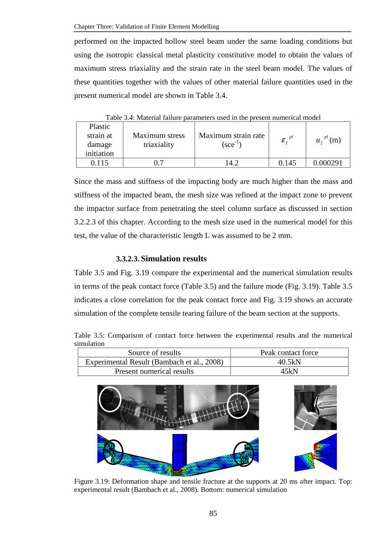
Chapter Three: Validation of Finite Element Modelling
85
performed on the impacted hollow steel beam under the same loading conditions but
using the isotropic classical metal plasticity constitutive model to obtain the values of
maximum stress triaxiality and the strain rate in the steel beam model. The values of
these quantities together with the values of other material failure quantities used in the
present numerical model are shown in Table 3.4.
Table 3.4: Material failure parameters used in the present numerical model
Plastic strain at damage initiation
Maximum stress triaxiality
Maximum strain rate (sce-1)
plfε pl
fu (m)
0.115 0.7 14.2 0.145 0.000291 Since the mass and stiffness of the impacting body are much higher than the mass and
stiffness of the impacted beam, the mesh size was refined at the impact zone to prevent
the impactor surface from penetrating the steel column surface as discussed in section
3.2.2.3 of this chapter. According to the mesh size used in the numerical model for this
test, the value of the characteristic length L was assumed to be 2 mm.
3.3.2.3. Simulation results
Table 3.5 and Fig. 3.19 compare the experimental and the numerical simulation results
in terms of the peak contact force (Table 3.5) and the failure mode (Fig. 3.19). Table 3.5
indicates a close correlation for the peak contact force and Fig. 3.19 shows an accurate
simulation of the complete tensile tearing failure of the beam section at the supports.
Table 3.5: Comparison of contact force between the experimental results and the numerical simulation
Source of results Peak contact force Experimental Result (Bambach et al., 2008) 40.5kN
Present numerical results 45kN
Figure 3.19: Deformation shape and tensile fracture at the supports at 20 ms after impact. Top: experimental result (Bambach et al., 2008). Bottom: numerical simulation
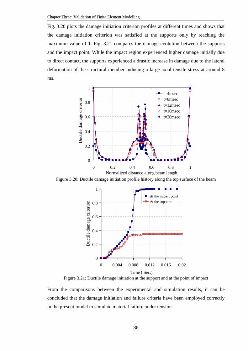
Chapter Three: Validation of Finite Element Modelling
86
Fig. 3.20 plots the damage initiation criterion profiles at different times and shows that
the damage initiation criterion was satisfied at the supports only by reaching the
maximum value of 1. Fig. 3.21 compares the damage evolution between the supports
and the impact point. While the impact region experienced higher damage initially due
to direct contact, the supports experienced a drastic increase in damage due to the lateral
deformation of the structural member inducing a large axial tensile stress at around 8
ms.
0
0.2
0.4
0.6
0.8
1
0 0.2 0.4 0.6 0.8 1Normalized distance along beam length
Duc
tile
da
ma
ge c
rite
rion
t=4msect=8msect=12msect=16msect=20msec
Figure 3.20: Ductile damage initiation profile history along the top surface of the beam
0
0.2
0.4
0.6
0.8
1
0 0.004 0.008 0.012 0.016 0.02
Time ( Sec.)
Du
ctile
dam
age
crite
rio
n At the impact point
At the supports
Figure 3.21: Ductile damage initiation at the support and at the point of impact
From the comparisons between the experimental and simulation results, it can be
concluded that the damage initiation and failure criteria have been employed correctly
in the present model to simulate material failure under tension.
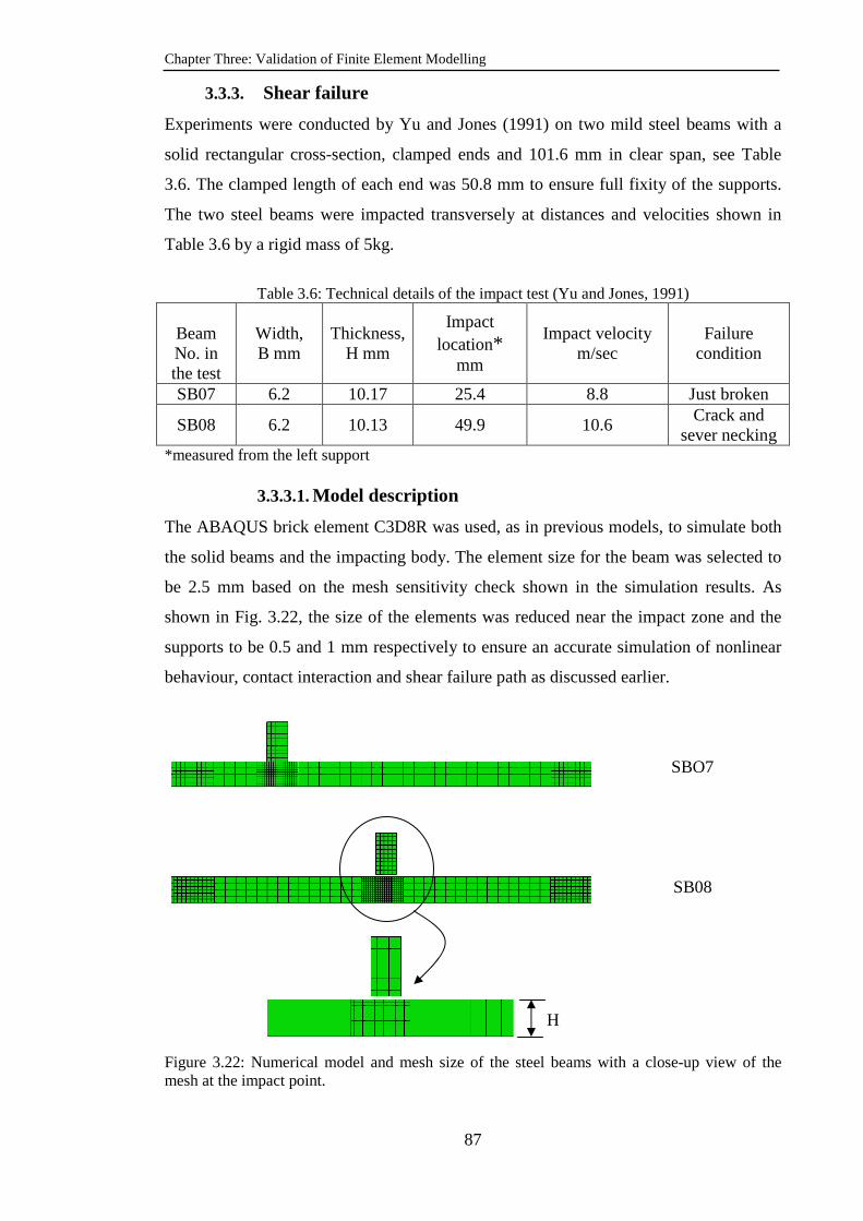
Chapter Three: Validation of Finite Element Modelling
87
3.3.3. Shear failure
Experiments were conducted by Yu and Jones (1991) on two mild steel beams with a
solid rectangular cross-section, clamped ends and 101.6 mm in clear span, see Table
3.6. The clamped length of each end was 50.8 mm to ensure full fixity of the supports.
The two steel beams were impacted transversely at distances and velocities shown in
Table 3.6 by a rigid mass of 5kg.
Table 3.6: Technical details of the impact test (Yu and Jones, 1991)
Beam No. in the test
Width, B mm
Thickness, H mm
Impact location*
mm
Impact velocity m/sec
Failure condition
SB07 6.2 10.17 25.4 8.8 Just broken
SB08 6.2 10.13 49.9 10.6 Crack and
sever necking *measured from the left support
3.3.3.1. Model description
The ABAQUS brick element C3D8R was used, as in previous models, to simulate both
the solid beams and the impacting body. The element size for the beam was selected to
be 2.5 mm based on the mesh sensitivity check shown in the simulation results. As
shown in Fig. 3.22, the size of the elements was reduced near the impact zone and the
supports to be 0.5 and 1 mm respectively to ensure an accurate simulation of nonlinear
behaviour, contact interaction and shear failure path as discussed earlier.
SBO7
SB08
Figure 3.22: Numerical model and mesh size of the steel beams with a close-up view of the mesh at the impact point.
H

Chapter Three: Validation of Finite Element Modelling
88
Fig. 3.23 shows the true stress-strain relationship of the mild steel recorded from the
experimental test (Yu and Jones, 1991). The classical metal (Mises) plasticity model
available in ABAQUS/Explicit was used to simulate the material behaviour with
isotropic strain hardening and strain rate effects. The strain rate effects were described
by employing the Cowper-Symonds equation with material parameters D=1.05×10⁷ s-1
and q = 8.3 (Yu and Jones, 1991, Yu and Jones, 1997). The values of D and q have been
chosen by Liu and Jones to describe the strain rate-sensitive behaviour of the steel
material to fit the true stress- strain curve recorded from the experimental tests for
different strain rates (Yu and Jones, 1991, Yu and Jones, 1997). The same contact
interaction model as in the previous simulations was used to simulate the contact
between the rigid mass and the solid beam except that, in the current model, the
tangential behaviour of the contact was assumed to be frictionless, based on the
experimental observation that slipping occurred during the tests between the impacting
mass and the steel beam at the impact zone (Yu and Jones, 1991). Other properties
(steel density, modulus of elasticity and Poisson’s ratio) were the same as in previous
simulations.
Figure 3.23: True stress-true strain curve of steel plastic (Yu and Jones, 1991)
3.3.3.2. Modelling of shear failure
For this exercise, the damage initiation criterion was described in terms of the
equivalent plastic strain at the onset of shear damage (pl
Sε ). Table 3.7 presents the
values of these quantities used in the simulation.
2.0E+08
3.5E+08
5.0E+08
6.5E+08
8.0E+08
0 0.2 0.4 0.6 0.8 1Plastic strain
Tru
e pl
astic
str
ess Damage initiation
Damage propagation
=plSε 0.17 =pl
fε 0.83

Chapter Three: Validation of Finite Element Modelling
89
Table 3.7: Material failure parameters used in the present numerical model
Plastic strain at damage initiation
Maximum shear stress
ratio
Maximum strain rate (sce-1)
plfε
plfu (m)
0.172 1.8 120 0.83 0.000415
3.3.3.3. Simulation results
A mesh sensitive analysis was carried out firstly to select the optimum mesh sizes at the
impact zone, the supports and the rest of the beam as shown in Fig. 3.22. Fig. 3.24
compares the numerical maximum transverse displacement history at the impact point
of steel beam SB07 with the experimental test results for different mesh sizes. It can be
seen from this figure that the transverse displacement history of the impacted beam is
more sensitive to the mesh size at the impact zone and the support than to the rest of the
beam since most stresses and deformations occurred at these locations. Differences in
numerical simulation results are small for the different mesh sizes used, confirming that
the numerical simulation results are not mesh sensitive. Excellent matching can be seen
between the experimental results and the numerical results corresponding to the mesh
sizes shown in Fig. 3.22 (0.5mm and 1mm at impact zone and the supports respectively
and 2.5 at the rest of the beam). The maximum displacement in both results was
16.2mm and both histories indicate that no failure was experienced in the beam. The
maximum transverse displacement was either maintained constantly after 3 msec. as in
the present numerical simulation or slightly decreased as in the experimental test.
Figure 3.24: Comparison of the displacement at the impact point of the steel beam SB07 between the experimental results (Yu and Jones, 1991) and the present numerical simulation
0.0E+00
3.0E-03
6.0E-03
9.0E-03
1.2E-02
1.5E-02
1.8E-02
0.E+00 1.E-03 2.E-03 3.E-03 4.E-03 5.E-03
Time (Sec.)
Dis
plac
emen
t at t
he im
pact
poi
nt (
m)
Experimetal results
Impact zone=0.5mm,supports=1mm, the rest=2.5mmImpact zone=1mm,supports=2mm, the rest=2.5mmImpact zone=2.5mm,supports=2.5mm, the rest=2.5mmImpact zone=5mm,supports=5mm, others=5mmImpact zone=1mm,supports=2mm,the rest=5mm
ABAQUS results

Chapter Three: Validation of Finite Element Modelling
90
Fig. 3.25 shows the deformed shapes of the steel specimen SB08 after complete shear
failure from both the test and the present numerical simulation. Good agreement can be
seen between the two shapes in terms of the location and angle of the shear failure
surface. In fact, correlation between the results is highly satisfying. Table 3.8 compares
the maximum permanent transverse deformation of the same beam between the present
numerical results, the experimental results of Yu and Jones (1991) and the numerical
results of Yu and Jones which did not incorporate failure simulation (Yu and Jones,
1997). Fig. 3.26 further compares the axial normal strain of the steel beam SB08
underneath the impact point obtained by the present numerical model with that recorded
experimentally by Yu and Jones (1991). Excellent agreement can be noticed throughout.
This exercise can be used to confirm the accuracy and efficiency of the present
numerical model to simulate shear failure mode.
Figure 3.25: Comparison of the deformation shape of the steel specimen SB08 after shear failure between the experimental test (Yu and Jones, 1991) (top) and the numerical simulation (bottom). Table 3.8: Comparison of the maximum transverse displacement of the steel specimen SB08 between the results from the present numerical simulation with the experimental results, (Yu
and Jones, 1991) and the numerical simulation results, (Yu and Jones, 1997)
Quantity Experiment,
(Yu and Jones, 1991)
Numerical, no failure criteria,(Yu and Jones, 1997)
Numerical, present study
maximum permanent transverse deformation (mm)
21.8 21.26 21.5
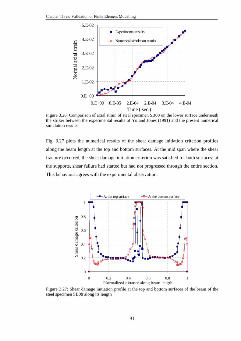
Chapter Three: Validation of Finite Element Modelling
91
0.E+00
1.E-02
2.E-02
3.E-02
4.E-02
5.E-02
0.E+00 8.E-05 2.E-04 2.E-04 3.E-04 4.E-04
Time ( sec.)
No
rmal
axi
al s
trai
n
Experimental results
Numerical simulation results
Figure 3.26: Comparison of axial strain of steel specimen SB08 on the lower surface underneath the striker between the experimental results of Yu and Jones (1991) and the present numerical simulation results
Fig. 3.27 plots the numerical results of the shear damage initiation criterion profiles
along the beam length at the top and bottom surfaces. At the mid span where the shear
fracture occurred, the shear damage initiation criterion was satisfied for both surfaces; at
the supports, shear failure had started but had not progressed through the entire section.
This behaviour agrees with the experimental observation.
0
0.2
0.4
0.6
0.8
1
0 0.2 0.4 0.6 0.8 1Normalized distance along beam length
Sh
ear
dam
age
crite
rio
n
At the top surface At the bottom surface
Figure 3.27: Shear damage initiation profile at the top and bottom surfaces of the beam of the steel specimen SB08 along its length
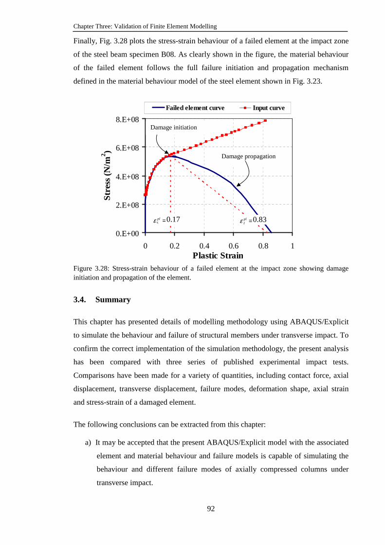
Chapter Three: Validation of Finite Element Modelling
92
Finally, Fig. 3.28 plots the stress-strain behaviour of a failed element at the impact zone
of the steel beam specimen B08. As clearly shown in the figure, the material behaviour
of the failed element follows the full failure initiation and propagation mechanism
defined in the material behaviour model of the steel element shown in Fig. 3.23.
Figure 3.28: Stress-strain behaviour of a failed element at the impact zone showing damage initiation and propagation of the element.
3.4. Summary
This chapter has presented details of modelling methodology using ABAQUS/Explicit
to simulate the behaviour and failure of structural members under transverse impact. To
confirm the correct implementation of the simulation methodology, the present analysis
has been compared with three series of published experimental impact tests.
Comparisons have been made for a variety of quantities, including contact force, axial
displacement, transverse displacement, failure modes, deformation shape, axial strain
and stress-strain of a damaged element.
The following conclusions can be extracted from this chapter:
a) It may be accepted that the present ABAQUS/Explicit model with the associated
element and material behaviour and failure models is capable of simulating the
behaviour and different failure modes of axially compressed columns under
transverse impact.
0.E+00
2.E+08
4.E+08
6.E+08
8.E+08
0 0.2 0.4 0.6 0.8 1Plastic Strain
Str
ess
(N/m
2 )Failed element curve Input curve
Damage initiation
=plSε 0.17 =pl
fε 0.83
Damage propagation
Chapter Three: Validation of Finite Element Modelling
93
b) The quasi-static analysis procedure in ABAQUS/Explicit can be used to simulate
the static force effect.
c) The results presented in this chapter may be considered to have provided an
extensive body of evidence that ABAQUS/Explicit is capable of modelling
axially loaded columns under transverse impact and that this model has been
correctly implemented in the current research.
d) It has been proven numerically that damping has only a minor effect on the
response and contact force of pre-compressed columns subjected to transverse
impact load (see Fig. 3.17). This conclusion has also been reached by other
researchers (Zeinoddini et al., 2008, Thilakarathna et al., 2010).
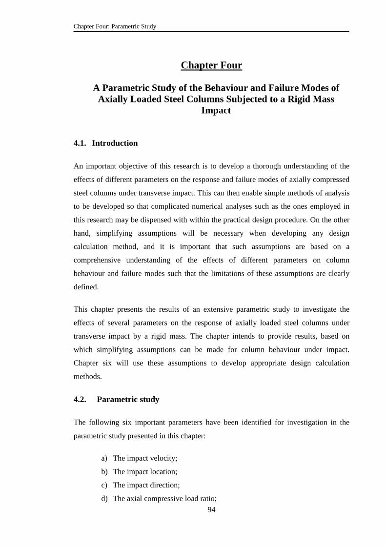
Chapter Four: Parametric Study
94
Chapter Four
A Parametric Study of the Behaviour and Failure Modes of Axially Loaded Steel Columns Subjected to a Rigid Mass
Impact
4.1. Introduction
An important objective of this research is to develop a thorough understanding of the
effects of different parameters on the response and failure modes of axially compressed
steel columns under transverse impact. This can then enable simple methods of analysis
to be developed so that complicated numerical analyses such as the ones employed in
this research may be dispensed with within the practical design procedure. On the other
hand, simplifying assumptions will be necessary when developing any design
calculation method, and it is important that such assumptions are based on a
comprehensive understanding of the effects of different parameters on column
behaviour and failure modes such that the limitations of these assumptions are clearly
defined.
This chapter presents the results of an extensive parametric study to investigate the
effects of several parameters on the response of axially loaded steel columns under
transverse impact by a rigid mass. The chapter intends to provide results, based on
which simplifying assumptions can be made for column behaviour under impact.
Chapter six will use these assumptions to develop appropriate design calculation
methods.
4.2. Parametric study
The following six important parameters have been identified for investigation in the
parametric study presented in this chapter:
a) The impact velocity;
b) The impact location;
c) The impact direction;
d) The axial compressive load ratio;

Chapter Four: Parametric Study
95
e) The column boundary condition;
f) The column slenderness ratio (section size and column length).
The following will describe in detail the numerical models for the steel column and the
impacting mass.
4.2.1. Steel columns
The parametric study used simply supported and propped cantilever H-section steel
columns designed according to the British Standard BS 5950: Part 1:2000 (BS, 2001) to
resist the total loads shown in Table 4.1. These loads represent the approximate total
axial compressive loads exerted on interior ground floor columns of 10 and 5 storeys
respectively of typical commercial steel buildings. To account for the slenderness effect,
two column lengths and sections were used. Table 4.1 lists the columns’ dimensions and
load carrying properties.
Table 4.1: Steel column properties used in the parametric study
Column
length
(m)
Column section
Slenderness
ratio ( )z z
kL
r −
Relative
slenderness
yz z
FkL
r Eλ
π− =
Boundary
condition
Design axial
compressive
load (kN)
4 UC
305×305×118
51.50 0.68 S.S 3800
36.05 0.476 Prop 4250
8 UC
356×406×340
76.9 1.02 S.S 6800
53.85 0.711 Prop 9400
S.S.: Simply supported; Prop: Propped cantilever.
The steel was assumed to be of grade S355 and the steel modulus of elasticity was
assumed to be 206000 N/mm2. The transverse impact load was mainly applied to cause
bending about the weak (minor) direction (z-z axis) of the steel column, which is
assumed to represent the most critical situation for design purposes. This assumption
has been confirmed in a separate parametric study in this chapter investigating the
effects of column impact from different directions.

Chapter Four: Parametric Study
96
4.2.1.1. Modelling properties
The solid element offered by ABAQUS/Explicit with reduced integration and hourglass
control C3D8R was used to model the geometrical behaviour of the steel column. To
achieve the required accuracy of the simulation, the thickness of both flanges and the
web of the column H-section were divided into four layers as shown in Fig 4.1 to
overcome the problems that could be raised from using the first order and the reduced
integration formulation of this element (SIMULIA, 2010b).
(A) (B)
Figure 4.1: Meshing technique used for the steel column: A) Longitudinal direction; B) Cross sectional direction for two steel column sections.
The material behaviour of the steel was modelled using an isotropic classical metal
plasticity model taking into account strain hardening and strain rate effects. The strain
rate effect was described by employing the Cowper-Symonds equation with material
parameters of D=40.4 s-1 and q=5 (Jones, 1997). The progressive damage and failure
model was used to account for the possibility of developing shear failure mode in the
steel column with the values of damage initiation criteria shown in Table 4.2. These
values were selected according to the uniaxial tensile test of S350 material shown in
Fig. 4.2. Other material failure quantities such maximum shear stress ratio, and
maximum strain rate were determined from a nonlinear finite element analysis carried
out before this simulation and these are presented in Table 4.2. It should be mentioned
that because this parametric study considered only columns with free axial movement,
tensile tearing failure is not likely to happen. Therefore, Table 4.2 only gives properties
for simulating transverse shear failure.

Chapter Four: Parametric Study
97
Figure 4.2: Assumed true stress-strain curve used to simulate S355 material behaviour in the
parametric study.
Table 4.2: Material shear failure parameters for S355 steel used in the parametric study
Plastic strain at damage
initiation
Maximum shear
stress ratio
Maximum strain rate
(sec-1)
plfε
plfu (m)
0.295 1.85 16.5 0.65 0.0065
The axial compressive load was applied on the steel column as a pressure load
distributed over the cross section area using the quasi-static analysis procedure
described in chapter three. The quasi-static analysis step was then followed by an
explicit dynamic step during which the rigid mass impacted the steel column at the
specified impact velocity and location by generating the contact interaction between the
mass and the steel column. The BOUNDARY option was used to specify the columns’
supporting condition by constraining and releasing the associated degree of freedom at
each column’s end.
4.2.1.2. Mesh size sensitivity
The sensitivity of the numerical simulation results against the column elements’ size
was firstly examined by determining the column’s minimum natural frequencies and
minimum buckling loads for different element sizes using the linear perturbation
analysis procedure available in ABAQUS (SIMULIA, 2010c) of UC 356×406×340 and
UC 305×305×118 columns with total lengths of 8 and 4 metres respectively. The
numerical values are compared with the corresponding theoretical values (Timoshenko,
1961) as listed in Table 4.3. It can be seen that the element sizes shown in Table 4.3 are
all appropriate for the static and global behaviour simulation of the columns.
2.0E+08
3.0E+08
4.0E+08
5.0E+08
6.0E+08
7.0E+08
8.0E+08
0 0.1 0.2 0.3 0.4 0.5 0.6 0.7Plastic strain
Tru
e pl
ast
ic s
tres
s
=plSε 0.295
=pl
fε 0.65

Chapter Four: Parametric Study
98
Table 4.3: Sensitivity of some static and dynamic results against the element size of the simply supported column model
Ele
men
t si
ze (
mm
)
UC 356×406×340, L= 8m UC 305×305×118, L= 4m
Frequency
(Numer./Theor.)
P(buckling)
(Numer./Theor.)
Frequency
(Numer./Theor)
P(buckling)
(Numer./Theor)
250 1.042693 1.190373 1.022045 1.054492
100 1.022265 1.045299 1.002676 1.013019
50 1.015226 1.031459 0.989474 0.988686
40 1.013849 1.028637 0.991444 0.992004
Afterwards, the effect of mesh size along the web height and over the flange length on
column behaviour was also verified by changing the number of divisions for each part
and plotting the corresponding column displacement histories. Fig. 4.3 (A and B) shows
the sensitivity of the results to each element size. It can be observed from this figure that
the column lateral displacement is more sensitive to the number of elements used for the
flange width than the web height. Dividing the flange width into 12 divisions gives
reasonable results compared to 18 divisions while element numbers along the web
height did not affect the results. This can be attributed to the direction of bending.
Therefore 12 and 10 divisions were used as minimum values for the flange width and
the web height respectively as previously shown in Fig.4.1
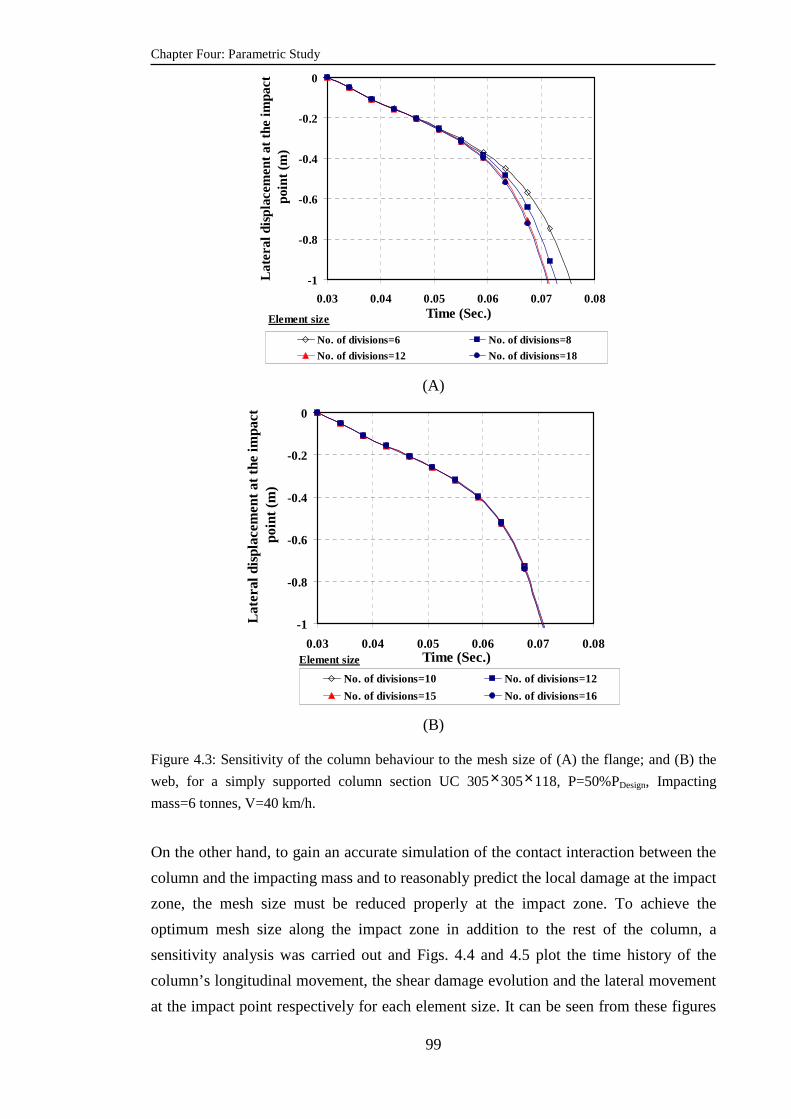
Chapter Four: Parametric Study
99
-1
-0.8
-0.6
-0.4
-0.2
0
0.03 0.04 0.05 0.06 0.07 0.08Time (Sec.)
Late
ral d
ispl
acem
ent a
t the
impa
ct
poin
t (m
)
No. of divisions=6 No. of divisions=8
No. of divisions=12 No. of divisions=18
Element size
(A)
-1
-0.8
-0.6
-0.4
-0.2
0
0.03 0.04 0.05 0.06 0.07 0.08Time (Sec.)
Late
ral d
ispl
acem
ent a
t the
impa
ct p
oint
(m
)
No. of divisions=10 No. of divisions=12
No. of divisions=15 No. of divisions=16
Element size
(B)
Figure 4.3: Sensitivity of the column behaviour to the mesh size of (A) the flange; and (B) the
web, for a simply supported column section UC 305×305×118, P=50%PDesign, Impacting
mass=6 tonnes, V=40 km/h.
On the other hand, to gain an accurate simulation of the contact interaction between the
column and the impacting mass and to reasonably predict the local damage at the impact
zone, the mesh size must be reduced properly at the impact zone. To achieve the
optimum mesh size along the impact zone in addition to the rest of the column, a
sensitivity analysis was carried out and Figs. 4.4 and 4.5 plot the time history of the
column’s longitudinal movement, the shear damage evolution and the lateral movement
at the impact point respectively for each element size. It can be seen from these figures
Chapter Four: Parametric Study
100
that a mesh size corresponding to 25600 elements for the steel column section UC
305×305×118 and 38845 elements for the steel column UC 356×406×340 (10 mm
within one meter of the impact point and 50 mm for the rest of the column) can be
adopted. Fig 4.6 shows such a mesh.
-1
-0.8
-0.6
-0.4
-0.2
0
0.08 0.11 0.14 0.18 0.21 0.25 0.28
Time (Sec.)
Axi
al d
ispl
ace
men
t a
t the
top
supp
ort
(m)
(A)
0
0.1
0.2
0.3
0.4
0.5
0.08 0.11 0.14 0.18 0.21 0.25 0.28Time (Sec.)
She
ar d
amag
e cr
iteri
on
(B)
At the impact zone: 150 mm, other parts: 250 mm. At the impact zone: 100 mm, other parts: 175 mm.
At the impact zone: 50 mm, other parts: 100 mm. At the impact zone: 25 mm, other parts: 75 mm.
At the impact zone: 15 mm, other parts: 65 mm. At the impact zone: 10 mm, other parts: 50 mm.
At the impact zone: 8 mm, other parts: 40 mm.
Element size
Figure 4.4: Sensitivity of the column axial displacement history, V=40 km/h (A) and the shear
damage history at the impact point; V=60 km/h (B) for different mesh sizes, column section UC
356×406×340, P=50%PDesign, Impacting mass=6 tonnes.

Chapter Four: Parametric Study
101
Figure 4.5: Sensitivity of the column lateral displacement history at the impact point for
different mesh sizes, column section UC 305×305×118, P=50%PDesign, Impacting mass=6
tonnes, V=40 km/h.
(A) Impact zone (10mm) (B) Rest of the column (50mm)
Figure 4.6: A close-up view of the element size of the steel column model adopted in the
parametric study
4.2.2. The impacting mass
Since the current study aims to investigate the behaviour and failure modes of axially
loaded steel columns under transverse impact, the emphasis will be on the column side
rather than the impactor side. Nevertheless, a brief description of the impartor properties
is required.
At the impact zone: 100 mm, other parts: 175 mm. At the impact zone: 50 mm, other parts: 100 mm.At the impact zone: 25 mm, other parts: 75 mm. At the impact zone: 15 mm, other parts: 50 mm.
At the impact zone: 10 mm, other parts: 50 mm. At the impact zone: 8 mm, other parts: 40 mm.At the impact zone: 5 mm, other parts: 25 mm.
Mesh size
-1
-0.8
-0.6
-0.4
-0.2
0
0.03 0.04 0.05 0.07 0.08 0.09 0.11
Time (Sec.)
Late
ral d
ispl
ace
men
t at th
e im
pact
poin
t (m
)

Chapter Four: Parametric Study
102
The impactor was assumed to be rigid mass with a cubic section of a dimensions
(0.5×1.5 ×0.3) m as shown in Fig. 4.7.
Figure 4.7: Shape and dimensions of the impactor used in the parametric study
Solid elements C3D8R were used to model the impactor body while its modulus of
elasticity was selected to make it behave as an almost rigid body so that all the kinetic
energy of the impact would be absorbed by the steel column without any contribution
from the impactor. On the other hand, the density of the impactor was adjusted to give
the required masses. The mesh size of the impactor was selected to be 100mm which
was intended to be larger than what was specified for the steel column at the impact
point (10mm) to prevent penetration of the master surface into the slave surface
(SIMULIA, 2010d), see Fig. 4.7 . The impact velocity was assigned to the mass as an
initial boundary condition using the PREDEFINED FIELD option in
ABAQUS/Explicit.
4.2.3. Modelling of contact
The contact pair algorithm discussed in chapter three was used to simulate the contact
interaction between the steel column and the impacting mass. The surface of the
impacting mass involved in the contact was defined in the numerical model as the
master surface while the steel column surface was considered the slave surface as
shown in Fig. 4.8. Hard contact was used to describe normal behaviour while the
penalty friction formulation was used for the tangential behaviour with a coefficient of
friction of 0.6 based on the nature of the contacted surfaces. The kinematic contact
enforcement method was also adopted in the contact model to detect the contact
between the two bodies with a small sliding formulation.
0.5 m
1.5m
0.3 m
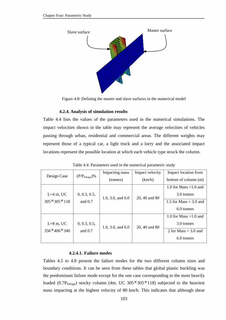
Chapter Four: Parametric Study
103
Figure 4.8: Defining the master and slave surfaces in the numerical model
4.2.4. Analysis of simulation results
Table 4.4 lists the values of the parameters used in the numerical simulations. The
impact velocities shown in the table may represent the average velocities of vehicles
passing through urban, residential and commercial areas. The different weights may
represent those of a typical car, a light truck and a lorry and the associated impact
locations represent the possible location at which each vehicle type struck the column.
Table 4.4: Parameters used in the numerical parametric study
Design Case (P/PDesign)% Impacting mass
(tonnes)
Impact velocity
(km/h)
Impact location from
bottom of column (m)
L=4 m, UC
305×305×118
0, 0.3, 0.5,
and 0.7 1.0, 3.0, and 6.0 20, 40 and 80
1.0 for Mass =1.0 and
3.0 tonnes
1.5 for Mass = 3.0 and
6.0 tonnes
L=8 m, UC
356×406×340
0, 0.3, 0.5,
and 0.7 1.0, 3.0, and 6.0 20, 40 and 80
1.0 for Mass =1.0 and
3.0 tonnes
2 for Mass = 3.0 and
6.0 tonnes
4.2.4.1. Failure modes
Tables 4.5 to 4.8 present the failure modes for the two different column sizes and
boundary conditions. It can be seen from these tables that global plastic buckling was
the predominant failure mode except for the one case corresponding to the most heavily
loaded (0.7PDesign) stocky column (4m, UC 305×305×118) subjected to the heaviest
mass impacting at the highest velocity of 80 km/h. This indicates that although shear
Master surface Slave surface

Chapter Four: Parametric Study
104
damage may occur to axially compressed steel columns under lateral impact, the
simulated scenario is unlikely to occur as it represents the very rare case of high impact
velocity/high impact mass/high axial load. In addition, it has been noticed that for this
particular case, it is most likely that shear failure occurred simultaneously with or just
before global buckling failure of the column. Therefore, this mode of failure (shear
failure) may be ignored when developing an analytical approach for quantifying the
critical failure conditions of steel columns in buildings located in urban areas.
Table 4.5: Failure modes for a simply supported column section UC 356×406×340
(P/PDesign)%
L=8m, Impact location =2 m L=8m, Impact Location =1m
Impact velocity (km/h) Impact velocity (km/h)
20 40 80 20 40 80
Mass
(tonnes)
Mass
(tonnes)
Mass
(tonnes)
Mass
(tonnes)
Mass
(tonnes)
Mass
(tonnes)
6 3 6 3 6 3 3 1 3 1 3 1
0.7 G N G G G G N N G N G N 0.5 N N G N G G N N N N G N 0.3 N N N N G G N N N N N N 0 N N N N N N N N N N N N
G=Global plastic failure, N=No failure.
Table 4.6: Failure modes for a propped cantilever column section UC 356×406×340
L=8m, Impact location =2 m L=8m, Impact Location =1m
(P/PDesign)%
Impact velocity (km/h) Impact velocity (km/h)
20 40 80 20 40 80
Mass
(tonnes)
Mass
(tonnes)
Mass
(tonnes)
Mass
(tonnes)
Mass
(tonnes)
Mass
(tonnes)
6 3 6 3 6 3 3 1 3 1 3 1
0.7 N N G N G G N N N N N N 0.5 N N G N G N N N N N N N 0.3 N N N N N N N N N N N N 0 N N N N N N N N N N N N
G=Global plastic failure, N=No failure.
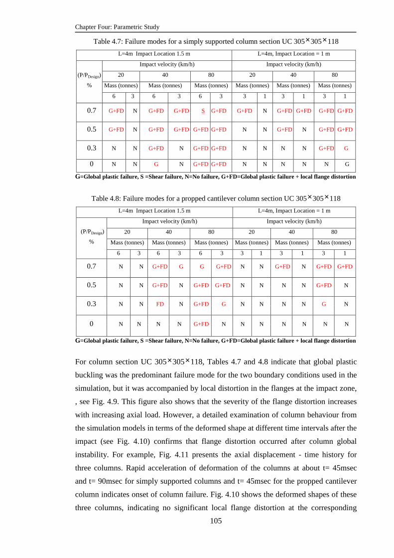
Chapter Four: Parametric Study
105
Table 4.7: Failure modes for a simply supported column section UC 305×305×118
L=4m Impact Location 1.5 m L=4m, Impact Location = 1 m
(P/PDesign)
%
Impact velocity (km/h) Impact velocity (km/h)
20 40 80 20 40 80
Mass (tonnes) Mass (tonnes) Mass (tonnes) Mass (tonnes) Mass (tonnes) Mass (tonnes)
6 3 6 3 6 3 3 1 3 1 3 1
0.7 G+FD N G+FD G+FD S G+FD G+FD N G+FD G+FD G+FD G+FD
0.5 G+FD N G+FD G+FD G+FD G+FD N N G+FD N G+FD G+FD
0.3 N N G+FD N G+FD G+FD N N N N G+FD G
0 N N G N G+FD G+FD N N N N N G
G=Global plastic failure, S =Shear failure, N=No failure, G+FD=Global plastic failure + local flange distortion
Table 4.8: Failure modes for a propped cantilever column section UC 305×305×118
L=4m Impact Location 1.5 m L=4m, Impact Location = 1 m
(P/PDesign)
%
Impact velocity (km/h) Impact velocity (km/h)
20 40 80 20 40 80
Mass (tonnes) Mass (tonnes) Mass (tonnes) Mass (tonnes) Mass (tonnes) Mass (tonnes)
6 3 6 3 6 3 3 1 3 1 3 1
0.7 N N G+FD G G G+FD N N G+FD N G+FD G+FD
0.5 N N G+FD N G+FD G+FD N N N N G+FD N
0.3 N N FD N G+FD G N N N N G N
0 N N N N G+FD N N N N N N N
G=Global plastic failure, S =Shear failure, N=No failure, G+FD=Global plastic failure + local flange distortion
For column section UC 305×305×118, Tables 4.7 and 4.8 indicate that global plastic
buckling was the predominant failure mode for the two boundary conditions used in the
simulation, but it was accompanied by local distortion in the flanges at the impact zone,
, see Fig. 4.9. This figure also shows that the severity of the flange distortion increases
with increasing axial load. However, a detailed examination of column behaviour from
the simulation models in terms of the deformed shape at different time intervals after the
impact (see Fig. 4.10) confirms that flange distortion occurred after column global
instability. For example, Fig. 4.11 presents the axial displacement - time history for
three columns. Rapid acceleration of deformation of the columns at about t= 45msec
and t= 90msec for simply supported columns and t= 45msec for the propped cantilever
column indicates onset of column failure. Fig. 4.10 shows the deformed shapes of these
three columns, indicating no significant local flange distortion at the corresponding
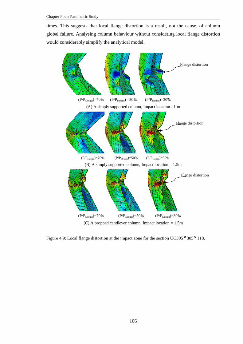
Chapter Four: Parametric Study
106
times. This suggests that local flange distortion is a result, not the cause, of column
global failure. Analysing column behaviour without considering local flange distortion
would considerably simplify the analytical model.
(P/PDesign)=70% (P/PDesign) =50% (P/PDesign)=30%
(A) A simply supported column, Impact location =1 m
(P/PDesign)=70% (P/PDesign)=50% (P/PDesign)=30%
(B) A simply supported column, Impact location = 1.5m
(P/PDesign)=70% (P/PDesign)=50% (P/PDesign)=30%
(C) A propped cantilever column, Impact location = 1.5m
Figure 4.9: Local flange distortion at the impact zone for the section UC305×305×118.
Flange distortion
Flange distortion
Flange distortion
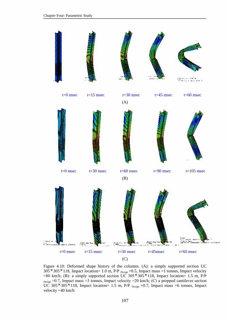
Chapter Four: Parametric Study
107
t=0 msec t=15 msec t=30 msec t=45 msec t=60 msec
(A)
t=0 msec t=30 msec t=60 msec t=90 msec t=105 msec
(B)
t=0 msec t=15 msec t=30 msec t=45msec t=60 msec
(C)
Figure 4.10: Deformed shape history of the columns. (A): a simply supported section UC 305×305×118, Impact location= 1.0 m, P/P Design =0.5, Impact mass =1 tonnes, Impact velocity =80 km/h; (B): a simply supported section UC 305×305×118, Impact location= 1.5 m, P/P Design =0.7, Impact mass =3 tonnes, Impact velocity =20 km/h; (C) a propped cantilever section
UC 305×305×118, Impact location= 1.5 m, P/P Design =0.7, Impact mass =6 tonnes, Impact velocity =40 km/h

Chapter Four: Parametric Study
108
-1
-0.8
-0.6
-0.4
-0.2
0
0.00 0.02 0.04 0.06 0.08 0.10 0.12
Time (Sec.)
Axi
al d
ispl
ecem
ent (
m)
P/P =0.5, V=80 km/h,Impact location = 1m
P/P =0.7, V=20 km/h,Impact location = 1.5m
P/P =0.7, V=40 km/h,Impact location = 1.5m
Design
Design
Design
Figure 4.11: The axial displacement history for the columns in Fig. 4.10
Figs. 4.12 to 4.14 show the shear damage profiles along the column height for the
simply supported and propped cantilever columns that are most vulnerable to shear
failure due to high impacting mass and velocity (Yu and Jones, 1991, Jones, 1997). It
can be seen that, apart from two cases which have shown a high tendency to local shear
failure (Fig. 4.12(A) and Fig. 4.13(B)), the damage initiation criteria were lower than
1.0. For the propped cantilever column, (see Fig. 4.14), it can be observed that the shear
damage criterion at the fixed support is greater than that at the impact point due to the
high stresses developed but the damage criteria is still below the failure limit. It is
apparent from these figures that the transverse shear failure is unlikely to occur in the
transversely impacted steel column when the transverse impact speed is within the range
of low to intermediate velocities.
(A) Impact location = 1 m, impact mass=3 tonnes (B) Impact location = 2 m, impact mass =6 tonnes
Figure 4.12: The shear damage initiation criterion profile along the column length for a simply supported column section UC 356×406×340, impact velocity = 80km/h
0
0.2
0.4
0.6
0.8
1
2 3 4 5 6 7 8Distance from the column top (m)
Dam
age
crite
rion
(P/P )=50%
(P/P )=70%Design
Design
0
0.2
0.4
0.6
0.8
1
2 3 4 5 6 7 8Distance from the column top (m)
Dam
age
crite
rion
(P/P )=0%(P/P )=30%
(P/P )=50%(P/P )=70%
Design
Design
Design
Design
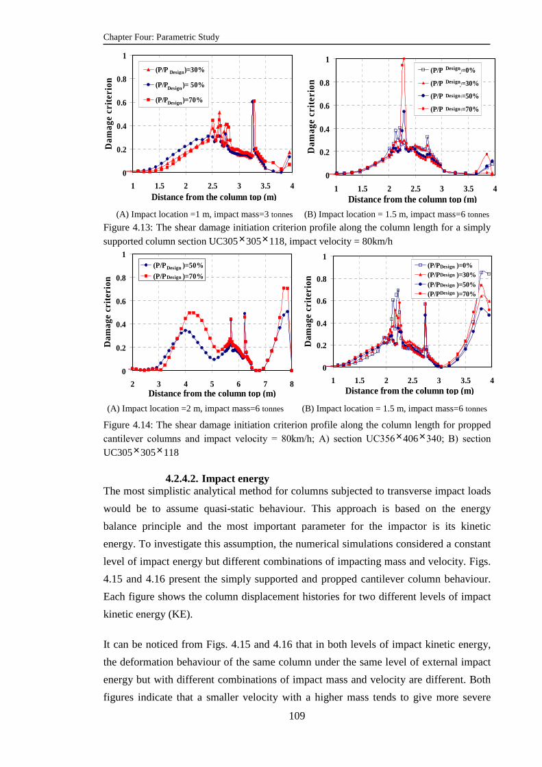
Chapter Four: Parametric Study
109
(A) Impact location =1 m, impact mass=3 tonnes (B) Impact location = 1.5 m, impact mass=6 tonnes Figure 4.13: The shear damage initiation criterion profile along the column length for a simply supported column section UC305×305×118, impact velocity = 80km/h
(A) Impact location =2 m, impact mass=6 tonnes (B) Impact location = 1.5 m, impact mass=6 tonnes
Figure 4.14: The shear damage initiation criterion profile along the column length for propped cantilever columns and impact velocity = 80km/h; A) section UC356×406×340; B) section
UC305×305×118
4.2.4.2. Impact energy The most simplistic analytical method for columns subjected to transverse impact loads
would be to assume quasi-static behaviour. This approach is based on the energy
balance principle and the most important parameter for the impactor is its kinetic
energy. To investigate this assumption, the numerical simulations considered a constant
level of impact energy but different combinations of impacting mass and velocity. Figs.
4.15 and 4.16 present the simply supported and propped cantilever column behaviour.
Each figure shows the column displacement histories for two different levels of impact
kinetic energy (KE).
It can be noticed from Figs. 4.15 and 4.16 that in both levels of impact kinetic energy,
the deformation behaviour of the same column under the same level of external impact
energy but with different combinations of impact mass and velocity are different. Both
figures indicate that a smaller velocity with a higher mass tends to give more severe
0
0.2
0.4
0.6
0.8
1
2 3 4 5 6 7 8Distance from the column top (m)
Dam
age
crite
rion
(P/P )=50%
(P/P )=70%Design
Design
0
0.2
0.4
0.6
0.8
1
1 1.5 2 2.5 3 3.5 4Distance from the column top (m)
Dam
age
crite
rion
(P/P )=0%(P/P )=30%(P/P )=50%(P/P )=70%
Design
Design
Design
Design
0
0.2
0.4
0.6
0.8
1
1 1.5 2 2.5 3 3.5 4Distance from the column top (m)
Dam
age
crite
rion
(P/P )=30%
(P/P )= 50%
(P/P )=70%
Design
Design
Design
0
0.2
0.4
0.6
0.8
1
1 1.5 2 2.5 3 3.5 4Distance from the column top (m)
Dam
age
crite
rion
(P/P )=0%
(P/P )=30%
(P/P )=50%
(P/P )=70%
Design
Design
Design
Design

Chapter Four: Parametric Study
110
column response (larger displacement). Nevertheless, whether or not the impacted
column would fail (which is the most important design decision) appears not to be very
sensitive to the different values of the impact mass and velocity as long as the external
impact energy is the same. For example, in Fig. 4.15(A), for the simply supported
column, the impact energy of 80 KJ was about 70% of the critical impact energy to
cause column failure. Therefore, none of the columns experienced failure. In contrast, in
Fig. 4.15(B), the impact energy of 117 KJ was at the level of the critical impact energy
of the column. All cases indicate column failure even though the case with the highest
velocity, 55km/hour, took a longer time for the column to reach failure. The same
behaviour can be observed in Fig. 4.16 which represents the same column section but
with a fixed support at the column base (propped cantilever).
0
0.08
0.16
0.24
0.32
0.4
0.03 0.06 0.10 0.14 0.18 0.22Time (Sec.)
Mid
spa
n di
spla
cem
ent (
m)
E=80 KJ, Mass= 1tonnes, V=45.6km/hE=80 KJ, Mass= 2tonnes, V=32.2km/hE=80 KJ, Mass= 3tonnes, V=26.3km/hE=80 KJ, Mass= 4tonnes, V=22.8km/hE=80 KJ, Mass= 6tonnes, V=18.6km/h
(A) P=50% of PDesign, KE=80 KJ
0
0.3
0.6
0.9
1.2
1.5
0.03 0.07 0.12 0.17 0.22 0.27
Time (Sec.)
Mid
sp
an
disp
lace
me
nt (
m) E117KJ, Mass=1tonnes,
V=55 km/h
E117KJ, Mass=2tonnes,V=39 km/h
E117KJ, Mass=3tonnes,V=32 km/h
E117KJ, Mass=4tonnes,V=28 km/h
E117KJ, Mass=6tonnes,V=22.5 km/h
(B) P=50% of PDesign, KE =117 KJ
Figure 4.15: Behaviour of the simply supported column (section UC 305×305×118, L=4m, impact location = 1m) under the same impact energy but with different combinations of impactor mass and velocity.
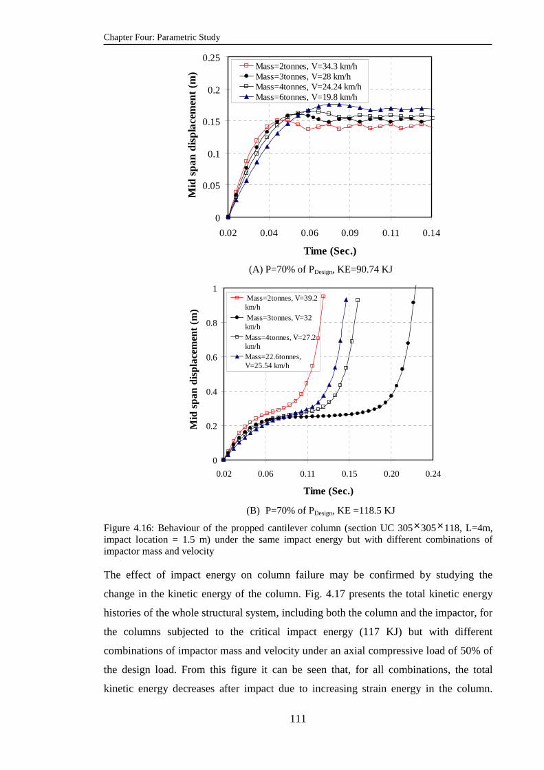
Chapter Four: Parametric Study
111
0
0.05
0.1
0.15
0.2
0.25
0.02 0.04 0.06 0.09 0.11 0.14
Time (Sec.)
Mid
spa
n di
spla
cem
ent (
m) Mass=2tonnes, V=34.3 km/h
Mass=3tonnes, V=28 km/hMass=4tonnes, V=24.24 km/hMass=6tonnes, V=19.8 km/h
(A) P=70% of PDesign, KE=90.74 KJ
0
0.2
0.4
0.6
0.8
1
0.02 0.06 0.11 0.15 0.20 0.24
Time (Sec.)
Mid
spa
n di
spla
cem
ent
(m)
Mass=2tonnes, V=39.2km/h
Mass=3tonnes, V=32km/h
Mass=4tonnes, V=27.2km/hMass=22.6tonnes,V=25.54 km/h
(B) P=70% of PDesign, KE =118.5 KJ
Figure 4.16: Behaviour of the propped cantilever column (section UC 305×305×118, L=4m, impact location = 1.5 m) under the same impact energy but with different combinations of impactor mass and velocity The effect of impact energy on column failure may be confirmed by studying the
change in the kinetic energy of the column. Fig. 4.17 presents the total kinetic energy
histories of the whole structural system, including both the column and the impactor, for
the columns subjected to the critical impact energy (117 KJ) but with different
combinations of impactor mass and velocity under an axial compressive load of 50% of
the design load. From this figure it can be seen that, for all combinations, the total
kinetic energy decreases after impact due to increasing strain energy in the column.
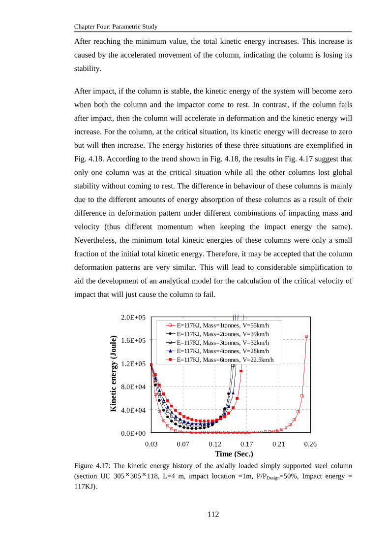
Chapter Four: Parametric Study
112
After reaching the minimum value, the total kinetic energy increases. This increase is
caused by the accelerated movement of the column, indicating the column is losing its
stability.
After impact, if the column is stable, the kinetic energy of the system will become zero
when both the column and the impactor come to rest. In contrast, if the column fails
after impact, then the column will accelerate in deformation and the kinetic energy will
increase. For the column, at the critical situation, its kinetic energy will decrease to zero
but will then increase. The energy histories of these three situations are exemplified in
Fig. 4.18. According to the trend shown in Fig. 4.18, the results in Fig. 4.17 suggest that
only one column was at the critical situation while all the other columns lost global
stability without coming to rest. The difference in behaviour of these columns is mainly
due to the different amounts of energy absorption of these columns as a result of their
difference in deformation pattern under different combinations of impacting mass and
velocity (thus different momentum when keeping the impact energy the same).
Nevertheless, the minimum total kinetic energies of these columns were only a small
fraction of the initial total kinetic energy. Therefore, it may be accepted that the column
deformation patterns are very similar. This will lead to considerable simplification to
aid the development of an analytical model for the calculation of the critical velocity of
impact that will just cause the column to fail.
0.0E+00
4.0E+04
8.0E+04
1.2E+05
1.6E+05
2.0E+05
0.03 0.07 0.12 0.17 0.21 0.26
Time (Sec.)
Kin
etic
ene
rgy
(Jou
le)
E=117KJ, Mass=1tonnes, V=55km/hE=117KJ, Mass=2tonnes, V=39km/hE=117KJ, Mass=3tonnes, V=32km/hE=117KJ, Mass=4tonnes, V=28km/hE=117KJ, Mass=6tonnes, V=22.5km/h
Figure 4.17: The kinetic energy history of the axially loaded simply supported steel column
(section UC 305×305×118, L=4 m, impact location =1m, P/PDesign=50%, Impact energy =
117KJ).

Chapter Four: Parametric Study
113
0.0E+00
4.0E+04
8.0E+04
1.2E+05
1.6E+05
2.0E+05
0 0.05 0.1 0.15 0.2 0.25
Time (Sec.)
Kin
etic
ene
rgy
(Jou
le)
E=117 KJ, just failure energy
E=139 KJ, over failure energy
E=96.5 KJ, no failure energy
Figure 4.18: Comparison of the total kinetic energy history of the columns without failure, at the
critical condition, with clear failures
4.2.4.3. Critical impact velocity
From the numerical simulations results presented in previous sections, it is possible to
establish the axial force - critical impact velocity relationship for a given column section
and length. Here, the critical velocity is defined as the minimum impact velocity that
causes the column to fail. This critical velocity is of particular interest in the design of
columns to transverse impact. Fig. 4.19 shows examples of column mid-height
displacement versus time relationship under different impact speeds and these were
used to obtain the critical velocity.
0
0.1
0.2
0.3
0.4
0.5
0.6
0 0.04 0.08 0.12 0.16 0.2Time (Sec.)
Mid
spa
n di
sple
cem
ent (m
)
V = 20 km/h
V = 40 km/h
V = 50 km/h
V = 55 km/h
V = 60 km/h
V =70 km/h
Figure 4.19: Column mid-height deformation history under different impact speeds, steel column height L=4 m, Impact mass= 1 tonnes, P/PDesign=50%, impact position =1m, for a simply support column
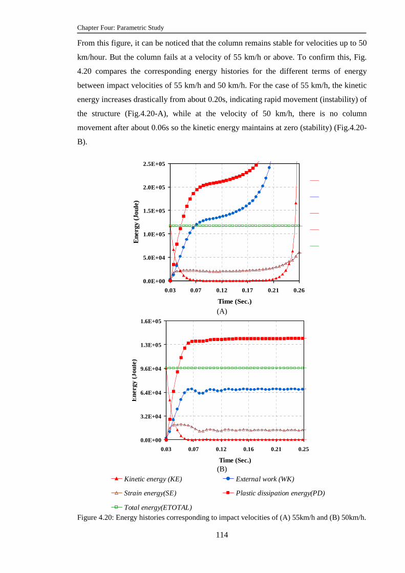
Chapter Four: Parametric Study
114
From this figure, it can be noticed that the column remains stable for velocities up to 50
km/hour. But the column fails at a velocity of 55 km/h or above. To confirm this, Fig.
4.20 compares the corresponding energy histories for the different terms of energy
between impact velocities of 55 km/h and 50 km/h. For the case of 55 km/h, the kinetic
energy increases drastically from about 0.20s, indicating rapid movement (instability) of
the structure (Fig.4.20-A), while at the velocity of 50 km/h, there is no column
movement after about 0.06s so the kinetic energy maintains at zero (stability) (Fig.4.20-
B).
0.0E+00
5.0E+04
1.0E+05
1.5E+05
2.0E+05
2.5E+05
0.03 0.07 0.12 0.17 0.21 0.26
Time (Sec.)
Ene
rgy
(Jou
le)
(A)
0.0E+00
3.2E+04
6.4E+04
9.6E+04
1.3E+05
1.6E+05
0.03 0.07 0.12 0.16 0.21 0.25
Time (Sec.)
Ene
rgy
(Jou
le)
(B)
Kinetic energy (KE) External work (WK)
Strain energy(SE) Plastic dissipation energy(PD)
Total energy(ETOTAL) Figure 4.20: Energy histories corresponding to impact velocities of (A) 55km/h and (B) 50km/h.

Chapter Four: Parametric Study
115
Using the same procedure, the axial force - critical impact velocity interaction curves
can be obtained for different levels of axial compressive load ratios and for the two
column boundary conditions investigated in this chapter as shown in the Figure 4.21.
(A) (B)
Figure 4.21: Axial force - critical impact velocity interaction curves of the steel columns used in
the parametric study: (A) section UC 356×406×340, L=8 m, impact mass=6tonnes, impact
location =2m); (B) section UC 305×305×118, L=4 m, impact mass=3tonnes, impact location
=1.5m)
4.2.4.4. Plastic hinge location
When developing analytical solutions to the transverse impact problem, it is necessary
to know where the plastic hinge forms so as to quantify the plastic dissipation energy of
the column. Fig. 4.22 shows how the relationship between the axial compressive load as
a percentage of the design load (vertical axis) and the location of the plastic hinge,
measured from the column base, as a percentage of the total column length, for columns
failed in global mode for the two column sections, two boundary conditions and
different impact locations. Here, additional numerical simulations were carried out
using an impact location at the middle of the span of each column section to cover the
effect of different possible impact locations on the location of the intermediate plastic
hinge. Fig. 4.22 (A and B) shows that the plastic hinge location is not significantly
affected by the axial load values or the impact location because it is always close to the
column mid-span (0.375-0.5)L for the simply supported columns and (0.5-0.65)L for
the propped cantilever columns. This is because when the column fails due to global
plastic instability, the deformation shape of the column is more likely to follow the first
mode for static buckling (Adachi et al., 2004, Sastranegara et al., 2006, Shope, 2006),
0.0
0.2
0.5
0.7
1.0
1.2
0 36 72 108 144 180
Critical impact velocity (km/h)
(P/P
Des
ign)
Simply supported
Propped cantilever
0
0.2
0.4
0.6
0.8
1
1.2
0 24 48 72 96 120
Critical Impact velocity (km/h)(P
/PD
esi
gn)
Simply supported
Propped cantilever
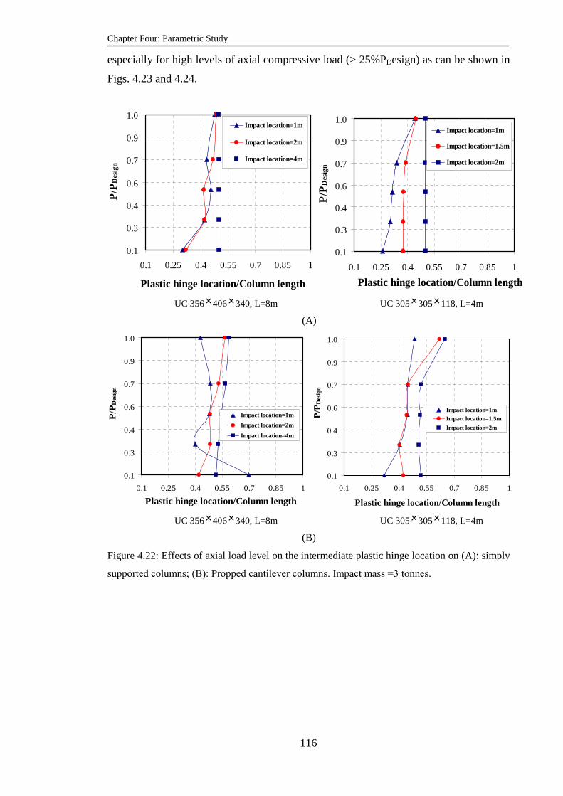
Chapter Four: Parametric Study
116
especially for high levels of axial compressive load (> 25%PDesign) as can be shown in
Figs. 4.23 and 4.24.
UC 356×406×340, L=8m UC 305×305×118, L=4m
(A)
UC 356×406×340, L=8m UC 305×305×118, L=4m
(B)
Figure 4.22: Effects of axial load level on the intermediate plastic hinge location on (A): simply
supported columns; (B): Propped cantilever columns. Impact mass =3 tonnes.
0.1
0.3
0.4
0.6
0.7
0.9
1.0
0.1 0.25 0.4 0.55 0.7 0.85 1
Plastic hinge location/Column length
P/P
Des
ign
Impact location=1m
Impact location=2m
Impact location=4m
0.1
0.3
0.4
0.6
0.7
0.9
1.0
0.1 0.25 0.4 0.55 0.7 0.85 1
Plastic hinge location/Column length
P/P
Des
ign
Impact location=1mImpact location=1.5m
Impact location=2m
0.1
0.3
0.4
0.6
0.7
0.9
1.0
0.1 0.25 0.4 0.55 0.7 0.85 1
Plastic hinge location/Column length
P/P
Des
ign
Impact location=1m
Impact location=2m
Impact location=4m
0.1
0.3
0.4
0.6
0.7
0.9
1.0
0.1 0.25 0.4 0.55 0.7 0.85 1
Plastic hinge location/Column length
P/P
Des
ign
Impact location=1m
Impact location=1.5m
Impact location=2m

Chapter Four: Parametric Study
117
(a) (b)
P=PDesign P=0.5PDesign P=0.1PDesign P=PDesign P=0.5PDesign
P=PDesign P=0.5PDesign P=0.1PDesign P=PDesign P=0.5PDesign P=0.1PDesign
(c) (d)
Figure 4.23: Collapse shapes showing the intermediate plastic hinge location for different axial
load ratios of simply supported columns (a) L= 8 m, impact location =2 m, Mass =6 tonnes; (b)
L= 8 m, impact location =1 m, Mass =3 Ton; (c) L= 4 m, impact location =1.5 m, Mass =6
tonnes; (d) L= 4 m, impact location=1 m, Mass = 3 tonnes
P=PDesign P=0.5PDesign P=0.1PDesign P=PDesign P=0.5PDesign P=0.1PDesign
(a) (b)
Figure 4.24: Collapse shapes showing the intermediate plastic hinge location for different axial
load ratios of propped cantilever columns; (a) L= 4 m, impact location =1.5 m, Mass =3 tonnes
(b) L= 8 m, impact location =2 m, Mass = 6 tonnes.

Chapter Four: Parametric Study
118
4.2.4.5. Effect of impact direction
The numerical simulations conducted in this chapter have assumed the impact direction
causing bending about the weak axis of the column to be the most critical situation in
terms of the column vulnerability to global failure. To validate this assumption, the
numerical simulations in this section considered two additional impact angles of 45 and
30 degrees as shown in Fig. 4.25. The axial load - critical impact velocity curves
resulting from these two cases are compared with that obtained from the 90 degree
impact as shown in Fig 4.26. This figure suggests that the critical velocity of the impact
on steel column subjected to 45 and 30 degrees’ impact are higher than that of 90
degrees’ impact. Therefore, for impact design, considering this direction (90 degrees)
should give more conservative results.
45o 30o 90o
Figure 4.25: 30, 45 and 90 degrees of impact
0.0
0.3
0.6
0.9
1.2
5 10 15 20 25 30
Critical impact velocity (km/h)
(P/P
Des
ign)
90 Degree Impact
45 Degree Impact
30 Degree Impact
Figure 4.26: Effect of impact direction on the critical impact velocity of a simply supported column section UC 305×305×118, Impact location=1.5m, Impact mass 6 tonnes.
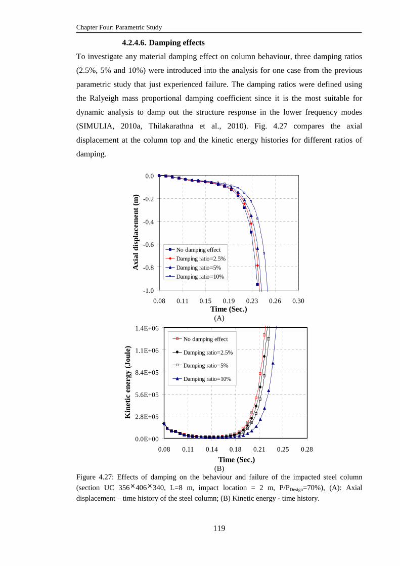
Chapter Four: Parametric Study
119
4.2.4.6. Damping effects
To investigate any material damping effect on column behaviour, three damping ratios
(2.5%, 5% and 10%) were introduced into the analysis for one case from the previous
parametric study that just experienced failure. The damping ratios were defined using
the Ralyeigh mass proportional damping coefficient since it is the most suitable for
dynamic analysis to damp out the structure response in the lower frequency modes
(SIMULIA, 2010a, Thilakarathna et al., 2010). Fig. 4.27 compares the axial
displacement at the column top and the kinetic energy histories for different ratios of
damping.
-1.0
-0.8
-0.6
-0.4
-0.2
0.0
0.08 0.11 0.15 0.19 0.23 0.26 0.30Time (Sec.)
Axi
al d
ispl
acem
ent (
m)
No damping effect
Damping ratio=2.5%
Damping ratio=5%
Damping ratio=10%
(A)
0.0E+00
2.8E+05
5.6E+05
8.4E+05
1.1E+06
1.4E+06
0.08 0.11 0.14 0.18 0.21 0.25 0.28
Time (Sec.)
Kin
etic
ene
rgy
(Jou
le)
No damping effect
Damping ratio=2.5%
Damping ratio=5%
Damping ratio=10%
(B)
Figure 4.27: Effects of damping on the behaviour and failure of the impacted steel column
(section UC 356×406×340, L=8 m, impact location = 2 m, P/PDesign=70%), (A): Axial
displacement – time history of the steel column; (B) Kinetic energy - time history.

Chapter Four: Parametric Study
120
It can be seen from Fig. 4.27, that the material damping effect is almost trivial. With
increasing damping, column failure was slightly delayed but not prevented. Fig. 4.28
shows column kinetic energies and the damping energies of the columns. Damping
energies increase only after the columns have failed, as indicated by the increase in
kinetic energies. Hence, it can be concluded that the effect of damping can be neglected
when determining the critical velocity of impact causing column failure.
0.0E+00
1.0E+05
2.0E+05
3.0E+05
4.0E+05
5.0E+05
0.08 0.11 0.15 0.18 0.22 0.25Time (Sec.)
Kin
etic
ene
rgy
(Jou
le)
KE (2.5% damping)
KE (5% damping)
KE (10% damping)
Damping energy(2.5% damping)
Damping energy(5% damping)
Damping energy(10% damping)
Figure 4.28: Kinetic energy and damping energy histories of the impacted steel columns with
the damping effect for the impacted steel column shown in Fig. 4.27.
4.2.4.7. Effects of strain hardening and strain rate
The numerical simulations presented in the previous sections have included strain
hardening and strain rate effects in the steel material behaviour. To investigate the
effects of these material properties on column behaviour, particularly the critical impact
velocity, numerical simulations were carried out in this section without considering
strain hardening and strain rate effects.
Fig. 4.29 (A and B) shows the effect of strain hardening on the axial load-critical impact
velocity curve of the column. The figure shows a large reduction in the critical impact
velocity values if the strain hardening effect is ignored for the steel section UC
305×305×118 (see Fig. 4.29(B)). For the steel section UC356×406×340, L=8m, no
remarkable effect can be noticed (see Fig. 4.29(A)). Whilst ignoring this beneficial
effect of strain hardening may give a conservative design, the results are inaccurate.
Chapter six will suggest a possible approach to incorporate this effect in the simplified
analytical method.

Chapter Four: Parametric Study
121
(A) (B)
Figure 4.29: Effect of strain hardening on critical impact velocity of the simply supported steel
column section (A) section UC 356×406×340, L=8m, impact mass=6tonnes, impact location
=2m); (B) section UC 305×305×118, L=4 m, impact mass=6tonnes, impact location =1.5m)
One the other hand, the effects of strain rate may be ignored because of the low strain
rate encountered in this type of impact. For example, Fig. 4.30 shows the maximum
strain rate along the column length for column section UC 356 ×406× 340 for a high
impact velocity of 90km/h. The maximum value is 0.1sec-1. At this value, the maximum
enhancement in the steel yield stress is 50% according to the Cowper-Symonds’ strain
rate model. Whilst this change from the static yield stress of 355N/mm2 is considerable,
the fact is that different rates occurring at different locations of the column would make
it very difficult to be incorporated in the simplified model. Since ignoring this effect
will result in a conservative design, the simplified model to be developed in chapter six
will not include this effect.
0.0
0.2
0.4
0.6
0.8
1.0
1.2
0 18 36 54 72 90
Critical impact velocity (km/h)
P/P
Des
ign
Without strain hardening
With strain hardening
0
0.2
0.4
0.6
0.8
1
1.2
0 10 20 30 40 50
Critical impact velocity(km/h)
P/P
Des
ign
Without strain hardening
With strain hardening
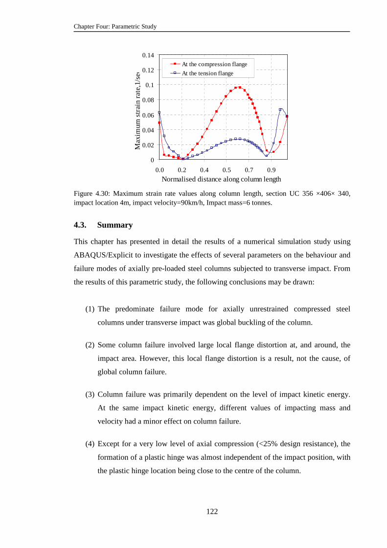
Chapter Four: Parametric Study
122
0
0.02
0.04
0.06
0.08
0.1
0.12
0.14
0.0 0.2 0.4 0.5 0.7 0.9
Normalised distance along column length
Ma
xim
um s
tra
in r
ate
,1/se
c
At the compression flange
At the tension flange
Figure 4.30: Maximum strain rate values along column length, section UC 356 ×406× 340, impact location 4m, impact velocity=90km/h, Impact mass=6 tonnes.
4.3. Summary This chapter has presented in detail the results of a numerical simulation study using
ABAQUS/Explicit to investigate the effects of several parameters on the behaviour and
failure modes of axially pre-loaded steel columns subjected to transverse impact. From
the results of this parametric study, the following conclusions may be drawn:
(1) The predominate failure mode for axially unrestrained compressed steel
columns under transverse impact was global buckling of the column.
(2) Some column failure involved large local flange distortion at, and around, the
impact area. However, this local flange distortion is a result, not the cause, of
global column failure.
(3) Column failure was primarily dependent on the level of impact kinetic energy.
At the same impact kinetic energy, different values of impacting mass and
velocity had a minor effect on column failure.
(4) Except for a very low level of axial compression (<25% design resistance), the
formation of a plastic hinge was almost independent of the impact position, with
the plastic hinge location being close to the centre of the column.
Chapter Four: Parametric Study
123
(5) The impact direction to cause bending of the column about the minor axis was
found to be the most critical direction of impact.
(6) Damping has little effect on the failure of the column and hence can be
neglected when calculating the critical impact velocity.
(7) Both strain hardening and strain rate have beneficial effects on column
behaviour and critical impact velocity. The effect of strain hardening will be
included in the development of a simplified method. However, the effect of
strain rate will be discarded because of the relatively low influence of this
parameter and the difficulty of implementing this effect in the simplified model.

Chapter Five: Simplified FE Vehicle Model
124
Chapter Five
A simplified FE Vehicle Model for Assessing the Vulnerability of
Axially Compressed Steel Columns Against Vehicle Frontal
Impact
5.1. Introduction
Vehicle impact mechanics have been an active research area for many years due to a
demand for vehicle crashworthiness and passenger safety. For this type of research, it is
necessary to understand the detailed mechanical behaviour of vehicles. However, when
studying column behaviour under a vehicle impact, as in the present research study, the
emphasis is on the impacted column rather than on the impacting vehicle, so it is only
necessary to develop an understanding of the global and external load resistance
characteristics of the vehicle frontal structure involved in such impact event.
The main objective of this chapter is to present and validate a simplified numerical
vehicle model that can be used to simulate the effects of vehicle frontal impact on steel
columns by using the commercial finite element code ABAQUS/Explicit. The
simplified numerical vehicle model treats the vehicle as a spring-mass system. This
model has, in fact, already been exploited by other researchers in the preliminary stages
of vehicle design and occupant safety assessment (Emori, 1968, Tani and Emori, 1970,
Kamal, 1970).
Simulating vehicle impact on a column using the spring-mass system requires defining
an accurate enough value of the vehicle stiffness against column impact. Vehicle
stiffness is a common term used as an important parameter in the field of vehicle safety
(Brell, 2005). Multiple definitions of vehicle stiffness have been established to describe
how to define and quantify this parameter and how to relate it to other important vehicle
parameters such as vehicle mass, vehicle velocity, vehicle deformation and vehicle
energy. Nevertheless, these definitions are all based on the assumption that the impacted
object has an infinite stiffness and width, and they cannot be directly used to express the
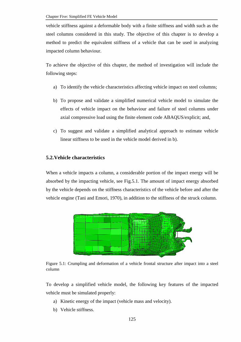
Chapter Five: Simplified FE Vehicle Model
125
vehicle stiffness against a deformable body with a finite stiffness and width such as the
steel columns considered in this study. The objective of this chapter is to develop a
method to predict the equivalent stiffness of a vehicle that can be used in analyzing
impacted column behaviour.
To achieve the objective of this chapter, the method of investigation will include the
following steps:
a) To identify the vehicle characteristics affecting vehicle impact on steel columns;
b) To propose and validate a simplified numerical vehicle model to simulate the
effects of vehicle impact on the behaviour and failure of steel columns under
axial compressive load using the finite element code ABAQUS/explicit; and,
c) To suggest and validate a simplified analytical approach to estimate vehicle
linear stiffness to be used in the vehicle model derived in b).
5.2. Vehicle characteristics
When a vehicle impacts a column, a considerable portion of the impact energy will be
absorbed by the impacting vehicle, see Fig.5.1. The amount of impact energy absorbed
by the vehicle depends on the stiffness characteristics of the vehicle before and after the
vehicle engine (Tani and Emori, 1970), in addition to the stiffness of the struck column.
Figure 5.1: Crumpling and deformation of a vehicle frontal structure after impact into a steel column
To develop a simplified vehicle model, the following key features of the impacted
vehicle must be simulated properly:
a) Kinetic energy of the impact (vehicle mass and velocity).
b) Vehicle stiffness.

Chapter Five: Simplified FE Vehicle Model
126
c) Contact interaction between the vehicle and the impacted structure.
Among all the previous techniques used to simulate vehicle impact, the spring-mass
model is deemed the most simplistic to represent the dynamic and load-deformation
characteristics of the vehicle. Since most of the previous experimental and analytical
studies have suggested a linear or bilinear relationship for the vehicle stiffness (Tani and
Emori, 1970, Milner et al., 2001), a single degree of freedom spring will be
implemented in the proposed simplified numerical vehicle model. Although numerical
modelling of the spring-mass system of one degree of freedom may be regarded as
simple, it is a highly challenging task when dealing with contact interaction and the
nonlinear load-deformation characteristics of the vehicle. The proposed model should
be able to generate the same kinetic energy that the original vehicle would generate at
the time of impact and it must also be able to follow the assumed load-deformation
characteristics of the vehicle under consideration up to the maximum impact force and
transfer this force to the impacted column through the contact zone.
5.3. Simplified vehicle model
The proposed simplified model is shown in Fig. 5.2, comprising a rigid body, a
nonlinear spring and a rigid massless surface. The mass of the rigid body represents the
total vehicle mass; the nonlinear spring represents the dynamic load-deformation
characteristics of the vehicle structure and the rigid surface simulates the contact
between the vehicle and the structure. The nonlinear spring was introduced in the model
using a NONLINEAR SPRING option in ABAQUS/Explicit with the load-deformation
characteristics defined in the input file of the model (SIMULIA, 2010a). The rigid
surface was defined as a DISCRETE RIGID SURFACE (SIMULIA, 2010b) which is
intended to prevent any energy absorption by the contact surface of the simplified
vehicle model. The curved contact surface has no sharp corners and ensures that the
contact point of the vehicle with the impacted structure does not cause any local stress
concentration in the structure.
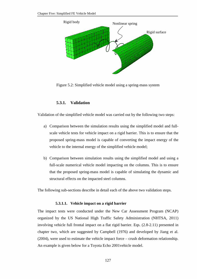
Chapter Five: Simplified FE Vehicle Model
127
Figure 5.2: Simplified vehicle model using a spring-mass system
5.3.1. Validation
Validation of the simplified vehicle model was carried out by the following two steps:
a) Comparison between the simulation results using the simplified model and full-
scale vehicle tests for vehicle impact on a rigid barrier. This is to ensure that the
proposed spring-mass model is capable of converting the impact energy of the
vehicle to the internal energy of the simplified vehicle model;
b) Comparison between simulation results using the simplified model and using a
full-scale numerical vehicle model impacting on the columns. This is to ensure
that the proposed spring-mass model is capable of simulating the dynamic and
structural effects on the impacted steel columns.
The following sub-sections describe in detail each of the above two validation steps.
5.3.1.1. Vehicle impact on a rigid barrier
The impact tests were conducted under the New Car Assessment Program (NCAP)
organized by the US National High Traffic Safety Administration (NHTSA, 2011)
involving vehicle full frontal impact on a flat rigid barrier. Eqs. (2.8-2.11) presented in
chapter two, which are suggested by Campbell (1976) and developed by Jiang et al.
(2004), were used to estimate the vehicle impact force – crush deformation relationship.
An example is given below for a Toyota Echo 2001vehicle model.
Nonlinear spring Rigid body
Rigid surface

Chapter Five: Simplified FE Vehicle Model
128
Determination of the stiffness coefficients and maximum impact force generated
from a full frontal crash of a Toyota Echo 2001 (first test in Table 5.1)
Total vehicle mass M = 1136 kg, impact velocity = 56.3km/h (15.63 m/s), the maximum
vehicle deformation (Cmax)= 0.464 m (NHTSA Test No. 3647), Wv=1.572 m. The
stiffness coefficient A and B can be determined using Eqs. 2.8 to 2.11 presented in
chapter two as follows(Campbell, 1976, Jiang et al., 2004):
2.2 /ob m s≈
1
max1 sec29
464.0
2.263.15 −≈−=−
=C
bVb o
1 1136 2.2 2946104.83 /
1.572o
v
Mb bA N m
W
× ×= = =
2 21 1136 29
607745.55 / /1.572v
MbB N m m
W
×= = =
Since the whole vehicle width is involved in the impact, the above calculated stiffness
coefficients must be multiplied by the vehicle width. Therefore:
46104.83 1.572 72476.8 ,
607745.55 1.572 955376 /
total
total
A N
B N m
= × =
= × =
The maximum impact force is:
max 72476.8 955376 0.464 515771F A B C N= + × = + × =
The above calculations can be used to define the stiffness characteristics of the spring
used in the simplified vehicle model. Fig. 5.3 shows the impact force – vehicle
deformation relationship assigned to the nonlinear spring to simulate vehicle impact on
a rigid crash barrier for the above example.
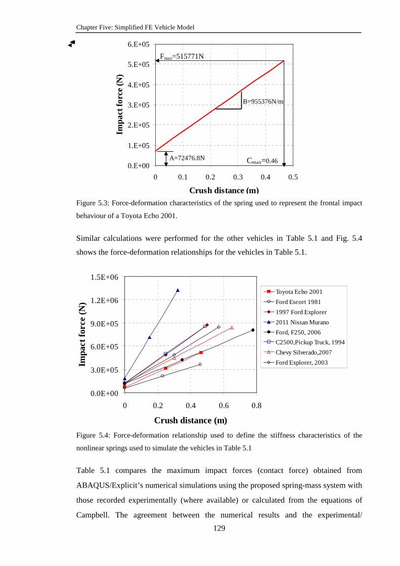
Chapter Five: Simplified FE Vehicle Model
129
Figure 5.3: Force-deformation characteristics of the spring used to represent the frontal impact
behaviour of a Toyota Echo 2001.
Similar calculations were performed for the other vehicles in Table 5.1 and Fig. 5.4
shows the force-deformation relationships for the vehicles in Table 5.1.
0.0E+00
3.0E+05
6.0E+05
9.0E+05
1.2E+06
1.5E+06
0 0.2 0.4 0.6 0.8
Crush distance (m)
Impa
ct fo
rce
(N)
Toyota Echo 2001
Ford Escort 1981
1997 Ford Explorer
2011 Nissan Murano
Ford, F250, 2006
C2500,Pickup Truck, 1994
Chevy Silverado,2007
Ford Explorer, 2003
Figure 5.4: Force-deformation relationship used to define the stiffness characteristics of the
nonlinear springs used to simulate the vehicles in Table 5.1
Table 5.1 compares the maximum impact forces (contact force) obtained from
ABAQUS/Explicit’s numerical simulations using the proposed spring-mass system with
those recorded experimentally (where available) or calculated from the equations of
Campbell. The agreement between the numerical results and the experimental/
0.E+00
1.E+05
2.E+05
3.E+05
4.E+05
5.E+05
6.E+05
0 0.1 0.2 0.3 0.4 0.5
Crush distance (m)
Impa
ct fo
rce
(N)
Fmax=515771N
Cmax=0.46
B=955376N/m
A=72476.8N
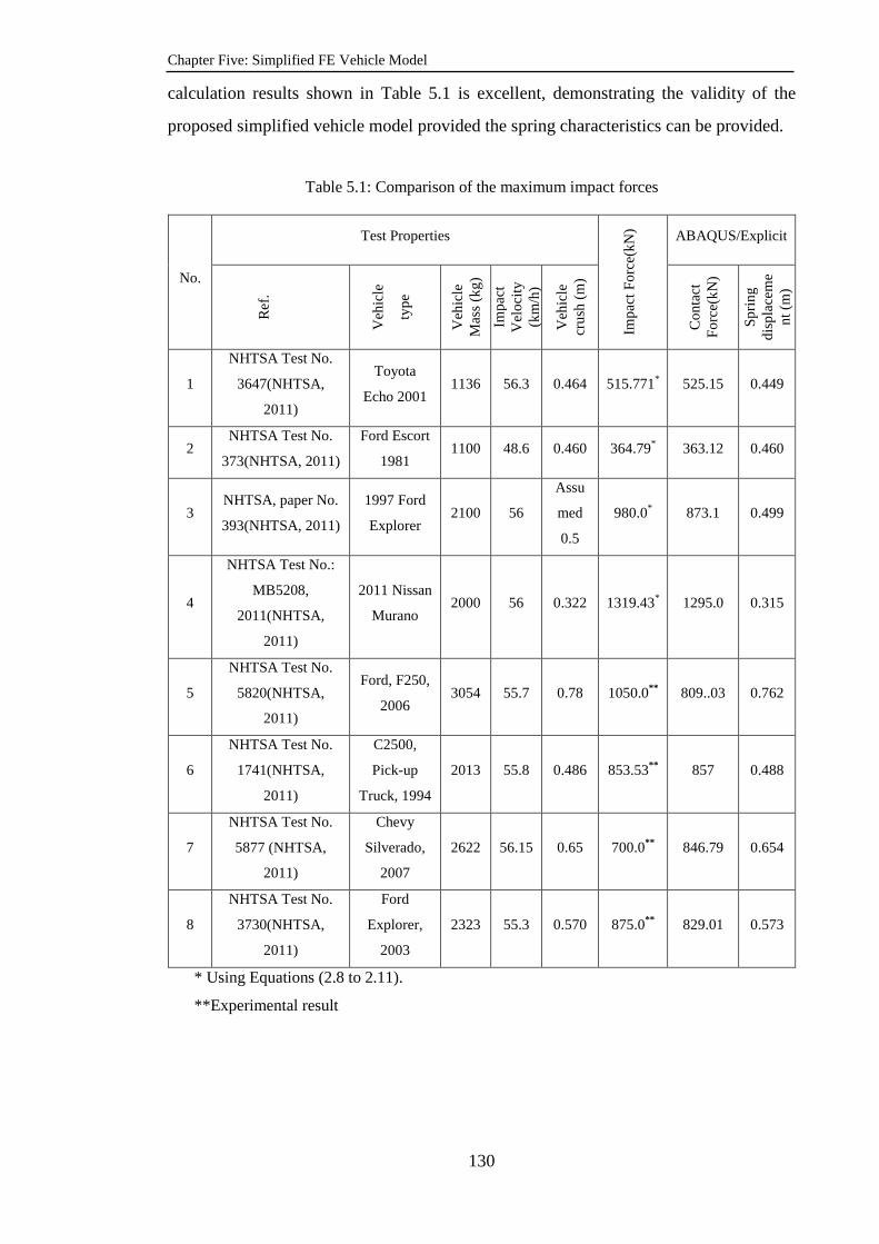
Chapter Five: Simplified FE Vehicle Model
130
calculation results shown in Table 5.1 is excellent, demonstrating the validity of the
proposed simplified vehicle model provided the spring characteristics can be provided.
Table 5.1: Comparison of the maximum impact forces
No.
Test Properties
Imp
act F
orc
e(kN
)
ABAQUS/Explicit
Ref
.
Veh
icle
typ
e
Veh
icle
M
ass
(kg
)
Imp
act
Vel
oci
ty
(km
/h)
Veh
icle
cr
ush
(m
)
Co
nta
ct
Fo
rce(
kN)
Sp
rin
g
dis
pla
cem
en
t (m
)
1
NHTSA Test No.
3647(NHTSA,
2011)
Toyota
Echo 2001 1136 56.3 0.464 515.771* 525.15 0.449
2 NHTSA Test No.
373(NHTSA, 2011)
Ford Escort
1981 1100 48.6 0.460 364.79* 363.12 0.460
3 NHTSA, paper No.
393(NHTSA, 2011)
1997 Ford
Explorer 2100 56
Assu
med
0.5
980.0* 873.1 0.499
4
NHTSA Test No.:
MB5208,
2011(NHTSA,
2011)
2011 Nissan
Murano 2000 56 0.322 1319.43* 1295.0 0.315
5
NHTSA Test No.
5820(NHTSA,
2011)
Ford, F250,
2006 3054 55.7 0.78 1050.0** 809..03 0.762
6
NHTSA Test No.
1741(NHTSA,
2011)
C2500,
Pick-up
Truck, 1994
2013 55.8 0.486 853.53** 857 0.488
7
NHTSA Test No.
5877 (NHTSA,
2011)
Chevy
Silverado,
2007
2622 56.15 0.65 700.0** 846.79 0.654
8
NHTSA Test No.
3730(NHTSA,
2011)
Ford
Explorer,
2003
2323 55.3 0.570 875.0** 829.01 0.573
* Using Equations (2.8 to 2.11).
**Experimental result
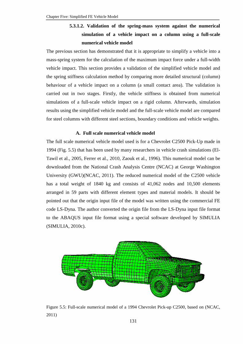
Chapter Five: Simplified FE Vehicle Model
131
5.3.1.2. Validation of the spring-mass system against the numerical
simulation of a vehicle impact on a column using a full-scale
numerical vehicle model
The previous section has demonstrated that it is appropriate to simplify a vehicle into a
mass-spring system for the calculation of the maximum impact force under a full-width
vehicle impact. This section provides a validation of the simplified vehicle model and
the spring stiffness calculation method by comparing more detailed structural (column)
behaviour of a vehicle impact on a column (a small contact area). The validation is
carried out in two stages. Firstly, the vehicle stiffness is obtained from numerical
simulations of a full-scale vehicle impact on a rigid column. Afterwards, simulation
results using the simplified vehicle model and the full-scale vehicle model are compared
for steel columns with different steel sections, boundary conditions and vehicle weights.
A. Full scale numerical vehicle model
The full scale numerical vehicle model used is for a Chevrolet C2500 Pick-Up made in
1994 (Fig. 5.5) that has been used by many researchers in vehicle crash simulations (El-
Tawil et al., 2005, Ferrer et al., 2010, Zaouk et al., 1996). This numerical model can be
downloaded from the National Crash Analysis Centre (NCAC) at George Washington
University (GWU)(NCAC, 2011). The reduced numerical model of the C2500 vehicle
has a total weight of 1840 kg and consists of 41,062 nodes and 10,500 elements
arranged in 59 parts with different element types and material models. It should be
pointed out that the origin input file of the model was written using the commercial FE
code LS-Dyna. The author converted the origin file from the LS-Dyna input file format
to the ABAQUS input file format using a special software developed by SIMULIA
(SIMULIA, 2010c).
Figure 5.5: Full-scale numerical model of a 1994 Chevrolet Pick-up C2500, based on (NCAC,
2011)

Chapter Five: Simplified FE Vehicle Model
132
Although the numerical model was developed and validated by NCAC, verification is
necessary to ensure that the ABAQUS version of this model is working properly and
that the conversion of the input file from LS-Dyna to ABAQUS/Explicit was performed
correctly. For this, a simulation of one test of the frontal vehicle impact on a flat and
rigid barrier conducted by NTHSA (test no. 1741) was performed. Details of the test are
available on the web site of NHTSA (NHTSA, 2011, NCAC, 2011). Fig. 5.6 compares
the author’s simulation result (contact force history) with the test result (NHTSA, 2011)
and the numerical simulation result by the National Crash Analysis Centre
(NCAC)(NCAC, 2011) which used a more detailed vehicle model (58313 element). The
agreement between the author’s simulation result and the test result is very good, better
than that achieved between the NCAC simulation result and the test result.
0.0E+00
3.2E+05
6.4E+05
9.6E+05
1.3E+06
1.6E+06
0 0.03 0.06 0.09 0.12 0.15
Time (Sec.)
Con
tact
For
ce (
N)
NHTSA Test
LS-Dyna-Detailed model(58313 element)
ABAQUS-Reduced mode(10500 element)
Figure 5.6: A comparison of the contact force history between the test (NHTSA, 2011), the
numerical simulation using a detailed FE vehicle model (NCAC, 2011) and the numerical
simulation using the reduced FE vehicle model of the present study
B. Validation for vehicle impact on steel columns
Three H-section steel columns were used in the numerical simulations. One column has
already been used in the numerical simulations described in chapter four (UC
305×305×118) and the other two columns were also designed according to the British
Standard BS 5950: Part 1:2000 in order to resist the total axial compressive loads
exerted on interior ground floor columns of artificial 10 storey, and 3 storey commercial
steel framed buildings. The resulting column sizes were UC 356×368×202 and UC
254×254×89. Columns with section sizes UC 305×305×118 and UC 254×254×89
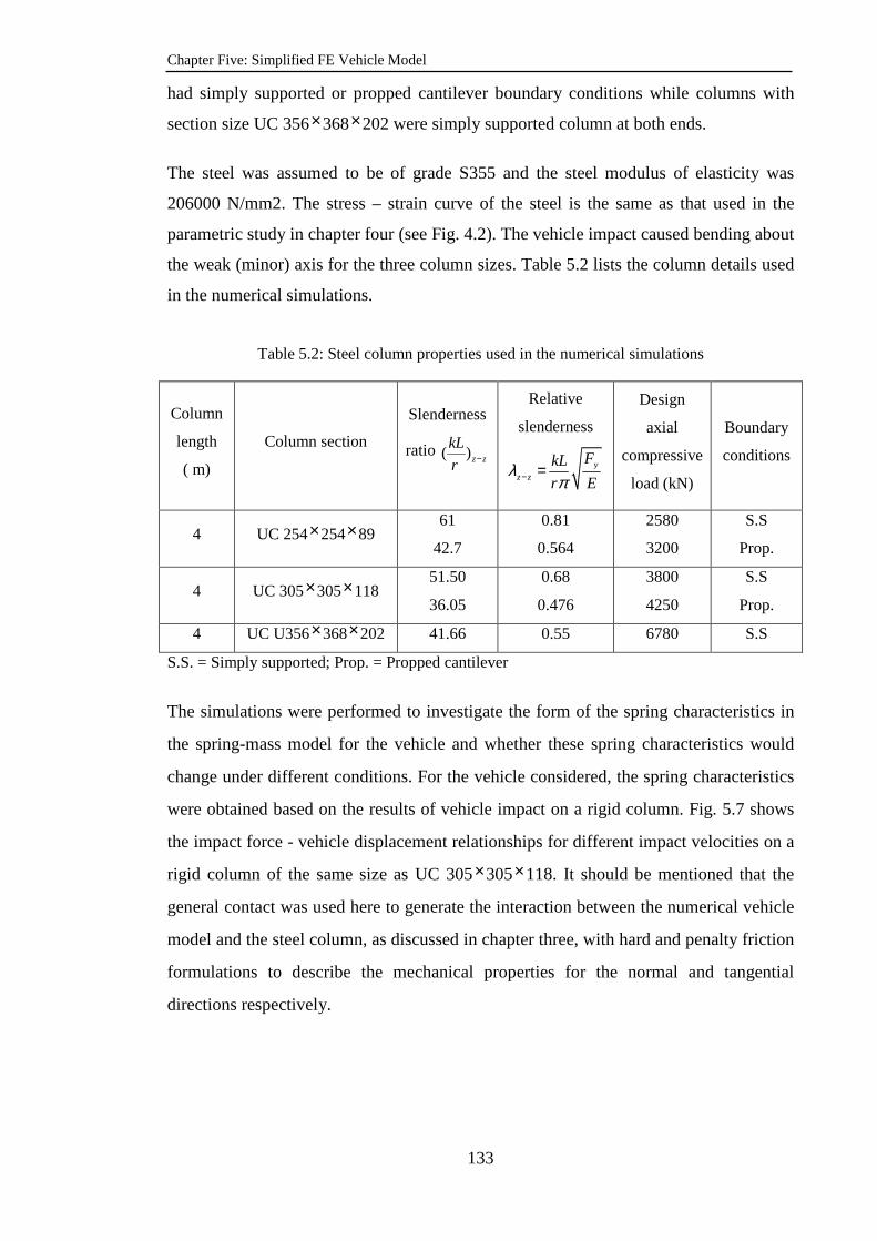
Chapter Five: Simplified FE Vehicle Model
133
had simply supported or propped cantilever boundary conditions while columns with
section size UC 356×368×202 were simply supported column at both ends.
The steel was assumed to be of grade S355 and the steel modulus of elasticity was
206000 N/mm2. The stress – strain curve of the steel is the same as that used in the
parametric study in chapter four (see Fig. 4.2). The vehicle impact caused bending about
the weak (minor) axis for the three column sizes. Table 5.2 lists the column details used
in the numerical simulations.
Table 5.2: Steel column properties used in the numerical simulations
Column
length
( m)
Column section
Slenderness
ratio ( )z z
kL
r −
Relative
slenderness
yz z
FkL
r Eλ
π− =
Design
axial
compressive
load (kN)
Boundary
conditions
4 UC 254×254×89 61
42.7
0.81
0.564
2580
3200
S.S
Prop.
4 UC 305×305×118 51.50
36.05
0.68
0.476
3800
4250
S.S
Prop.
4 UC U356×368×202 41.66 0.55 6780 S.S
S.S. = Simply supported; Prop. = Propped cantilever
The simulations were performed to investigate the form of the spring characteristics in
the spring-mass model for the vehicle and whether these spring characteristics would
change under different conditions. For the vehicle considered, the spring characteristics
were obtained based on the results of vehicle impact on a rigid column. Fig. 5.7 shows
the impact force - vehicle displacement relationships for different impact velocities on a
rigid column of the same size as UC 305×305×118. It should be mentioned that the
general contact was used here to generate the interaction between the numerical vehicle
model and the steel column, as discussed in chapter three, with hard and penalty friction
formulations to describe the mechanical properties for the normal and tangential
directions respectively.
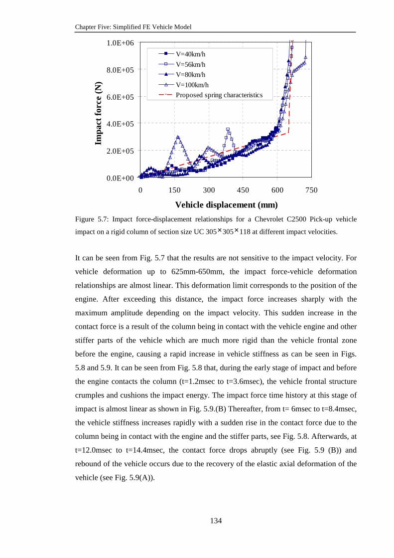
Chapter Five: Simplified FE Vehicle Model
134
0.0E+00
2.0E+05
4.0E+05
6.0E+05
8.0E+05
1.0E+06
0 150 300 450 600 750
Vehicle displacement (mm)
Impa
ct fo
rce
(N)
V=40km/h
V=56km/h
V=80km/h
V=100km/h
Proposed spring characteristics
Figure 5.7: Impact force-displacement relationships for a Chevrolet C2500 Pick-up vehicle
impact on a rigid column of section size UC 305×305×118 at different impact velocities.
It can be seen from Fig. 5.7 that the results are not sensitive to the impact velocity. For
vehicle deformation up to 625mm-650mm, the impact force-vehicle deformation
relationships are almost linear. This deformation limit corresponds to the position of the
engine. After exceeding this distance, the impact force increases sharply with the
maximum amplitude depending on the impact velocity. This sudden increase in the
contact force is a result of the column being in contact with the vehicle engine and other
stiffer parts of the vehicle which are much more rigid than the vehicle frontal zone
before the engine, causing a rapid increase in vehicle stiffness as can be seen in Figs.
5.8 and 5.9. It can be seen from Fig. 5.8 that, during the early stage of impact and before
the engine contacts the column (t=1.2msec to t=3.6msec), the vehicle frontal structure
crumples and cushions the impact energy. The impact force time history at this stage of
impact is almost linear as shown in Fig. 5.9.(B) Thereafter, from t= 6msec to t=8.4msec,
the vehicle stiffness increases rapidly with a sudden rise in the contact force due to the
column being in contact with the engine and the stiffer parts, see Fig. 5.8. Afterwards, at
t=12.0msec to t=14.4msec, the contact force drops abruptly (see Fig. 5.9 (B)) and
rebound of the vehicle occurs due to the recovery of the elastic axial deformation of the
vehicle (see Fig. 5.9(A)).
Chapter Five: Simplified FE Vehicle Model
135
t=1.2 ms t=3.6 ms
t=6ms t=8.4ms
t=12.0ms t=14.4 ms
Figure 5.8: A longitudinal cross section of the C2500 vehicle at different times of the impact
history showing the vehicle deformations before and after engine contact with a rigid column of
size UC 305×305×118 and the vehicle rebound thereafter, impact velocity = 56kN/m.
Vehicle engine

Chapter Five: Simplified FE Vehicle Model
136
(A) (B)
Figure 5.9: (A) Axial displacement and (B) contact force time histories of the C2500 vehicle
impacting a rigid column of size UC 305×305×118 at an impact velocity equal to 56km/h
Similarly, Fig. 5.10 shows the simulation results for the other two column sizes in Table
5.3 and the proposed bilinear spring impact force - deformation relationships. Although
Figs 5.7 and 5.10 indicate that the impact force - deformation relationship of the vehicle
is more close to a parabolic curve, a bilinear relationship has been assumed to represent
the vehicle force-displacement relationship as shown in Fig. 5.11. Assuming a bi-linear
stiffness relationship results in little loss of accuracy, but makes the vehicle load-
deformation relationship much easier to implement in both the numerical simulation
model and the analytical model.
Fig. 5.11 shows the idealized spring force - displacement relationship and Table 5.4 lists
the slopes (stiffness) for the first (K1) and second (K2) stages of the Chevrolet C2500
Pick-up vehicle. The changes in the stiffness values in Table 5.3 reflect the changes in
the contact area between the vehicle and the column, with a larger contact area giving
higher stiffness.
0
140
280
420
560
700
0 0.03 0.06 0.09 0.12 0.15
Time (Sec.)
Axi
al d
ispl
ace
men
t (m
m)
0.E+00
3.E+05
6.E+05
9.E+05
1.E+06
2.E+06
0 0.03 0.06 0.09 0.12 0.15
Time (Sec.)
Con
tact
forc
e(N
)
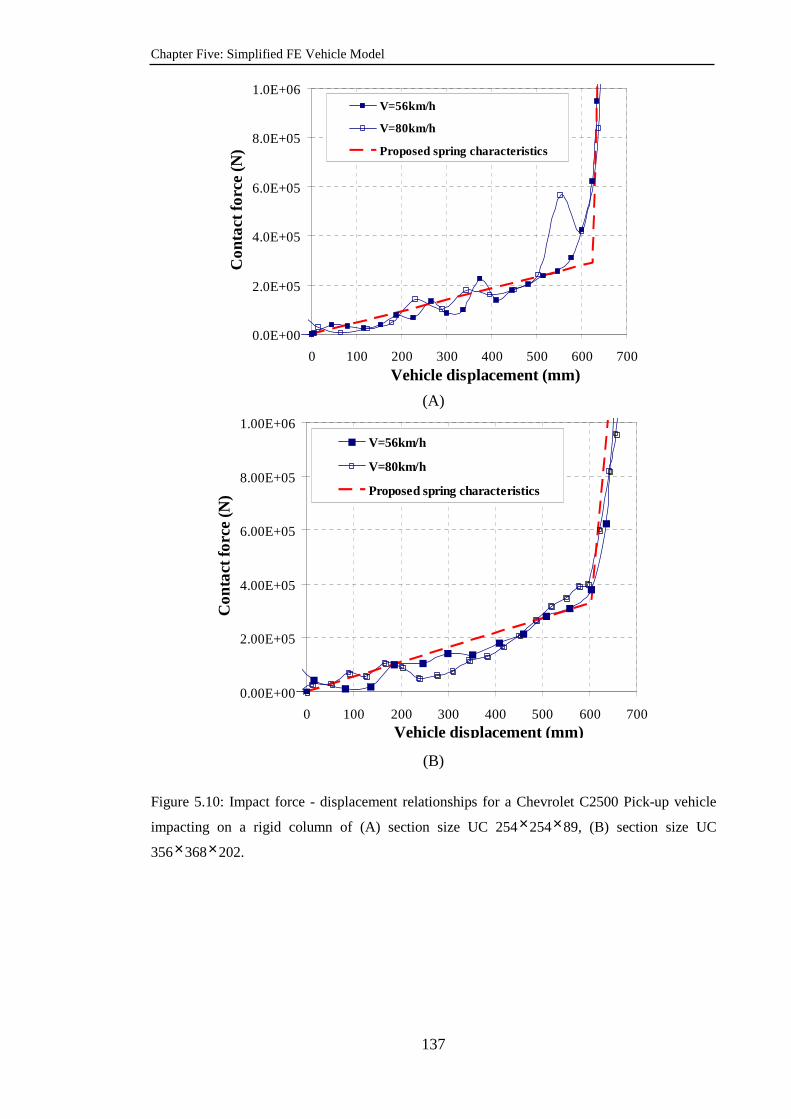
Chapter Five: Simplified FE Vehicle Model
137
0.0E+00
2.0E+05
4.0E+05
6.0E+05
8.0E+05
1.0E+06
0 100 200 300 400 500 600 700
Vehicle displacement (mm)
Con
tact
forc
e (N
)
V=56km/h
V=80km/h
Proposed spring characteristics
(A)
0.00E+00
2.00E+05
4.00E+05
6.00E+05
8.00E+05
1.00E+06
0 100 200 300 400 500 600 700Vehicle displacement (mm)
Con
tact
forc
e (N
)
V=56km/h
V=80km/h
Proposed spring characteristics
(B)
Figure 5.10: Impact force - displacement relationships for a Chevrolet C2500 Pick-up vehicle
impacting on a rigid column of (A) section size UC 254×254×89, (B) section size UC
356×368×202.
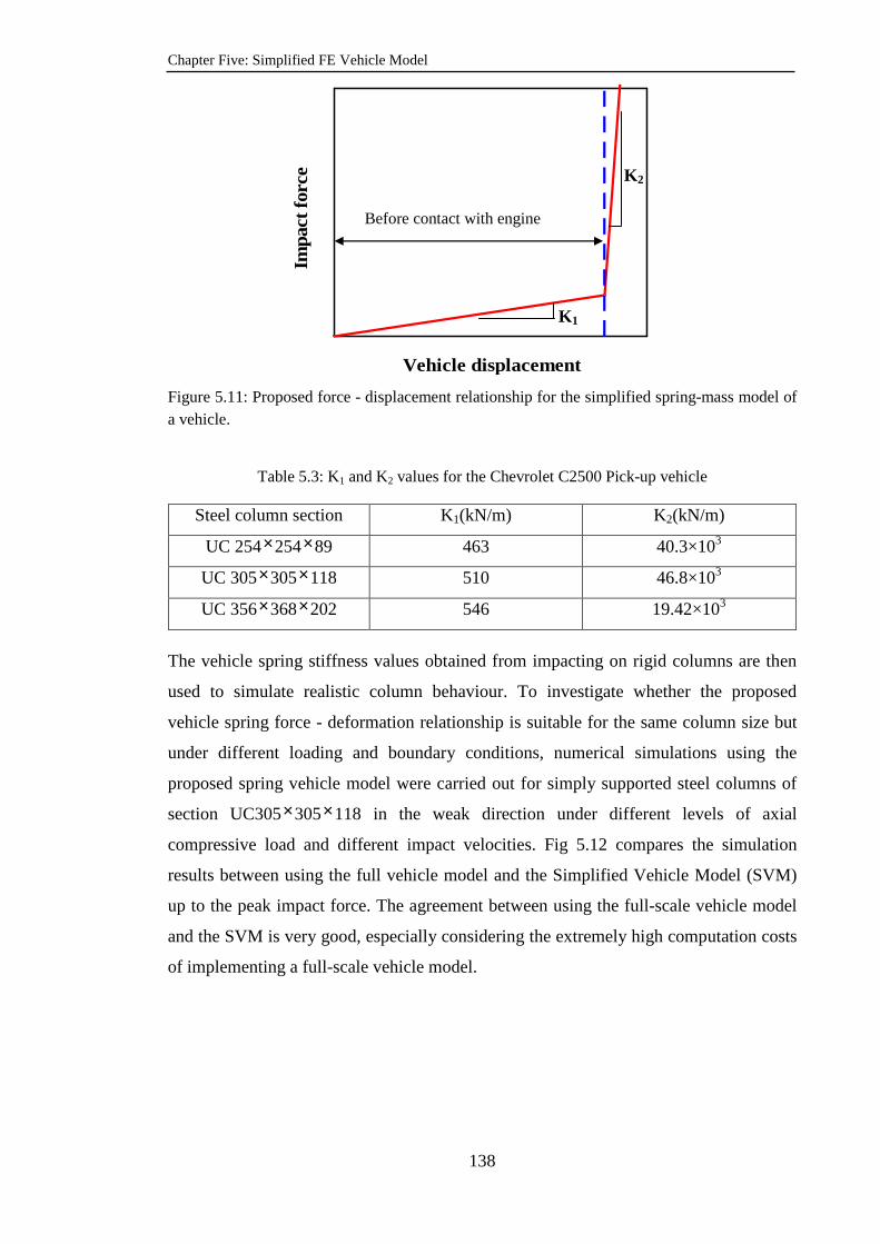
Chapter Five: Simplified FE Vehicle Model
138
Figure 5.11: Proposed force - displacement relationship for the simplified spring-mass model of a vehicle.
Table 5.3: K1 and K2 values for the Chevrolet C2500 Pick-up vehicle
Steel column section K1(kN/m) K2(kN/m)
UC 254×254×89 463 40.3×10³
UC 305×305×118 510 46.8×10³
UC 356×368×202 546 19.42×10³
The vehicle spring stiffness values obtained from impacting on rigid columns are then
used to simulate realistic column behaviour. To investigate whether the proposed
vehicle spring force - deformation relationship is suitable for the same column size but
under different loading and boundary conditions, numerical simulations using the
proposed spring vehicle model were carried out for simply supported steel columns of
section UC305×305×118 in the weak direction under different levels of axial
compressive load and different impact velocities. Fig 5.12 compares the simulation
results between using the full vehicle model and the Simplified Vehicle Model (SVM)
up to the peak impact force. The agreement between using the full-scale vehicle model
and the SVM is very good, especially considering the extremely high computation costs
of implementing a full-scale vehicle model.
Vehicle displacement
Impa
ct fo
rce
Before contact with engine
K1
K2
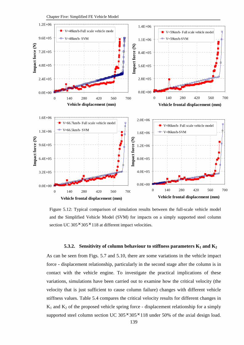
Chapter Five: Simplified FE Vehicle Model
139
Figure 5.12: Typical comparison of simulation results between the full-scale vehicle model
and the Simplified Vehicle Model (SVM) for impacts on a simply supported steel column
section UC 305×305×118 at different impact velocities.
5.3.2. Sensitivity of column behaviour to stiffness parameters K1 and K2
As can be seen from Figs. 5.7 and 5.10, there are some variations in the vehicle impact
force - displacement relationship, particularly in the second stage after the column is in
contact with the vehicle engine. To investigate the practical implications of these
variations, simulations have been carried out to examine how the critical velocity (the
velocity that is just sufficient to cause column failure) changes with different vehicle
stiffness values. Table 5.4 compares the critical velocity results for different changes in
K1 and K2 of the proposed vehicle spring force - displacement relationship for a simply
supported steel column section UC 305×305×118 under 50% of the axial design load.
0.0E+00
3.2E+05
6.4E+05
9.6E+05
1.3E+06
1.6E+06
0 140 280 420 560 700
Vehicle frontal displacement (mm)
Impa
ct fo
rce
(N)
V=66.7km/h- Full scale vehicle model
V=66.5km/h- SVM
0.0E+00
4.0E+05
8.0E+05
1.2E+06
1.6E+06
2.0E+06
0 140 280 420 560 700
Vehicle frontal displacement (mm)
Impa
ct fo
rce
(N)
V=86km/h- Full scale vehicle model
V=86km/h-SVM
0.0E+00
2.4E+05
4.8E+05
7.2E+05
9.6E+05
1.2E+06
0 140 280 420 560 700
Vehicle displacement (mm)
Impa
ct fo
rce
(N)
V=48km/h-Full scale vehicle mode
V=48km/h- SVM
0.0E+00
2.8E+05
5.6E+05
8.4E+05
1.1E+06
1.4E+06
0 140 280 420 560 700
Vehicle frontal displacement (mm)
Impa
ct fo
rce
(N)
V=59km/h- Full scale vehicle model
V=59km/h-SVM
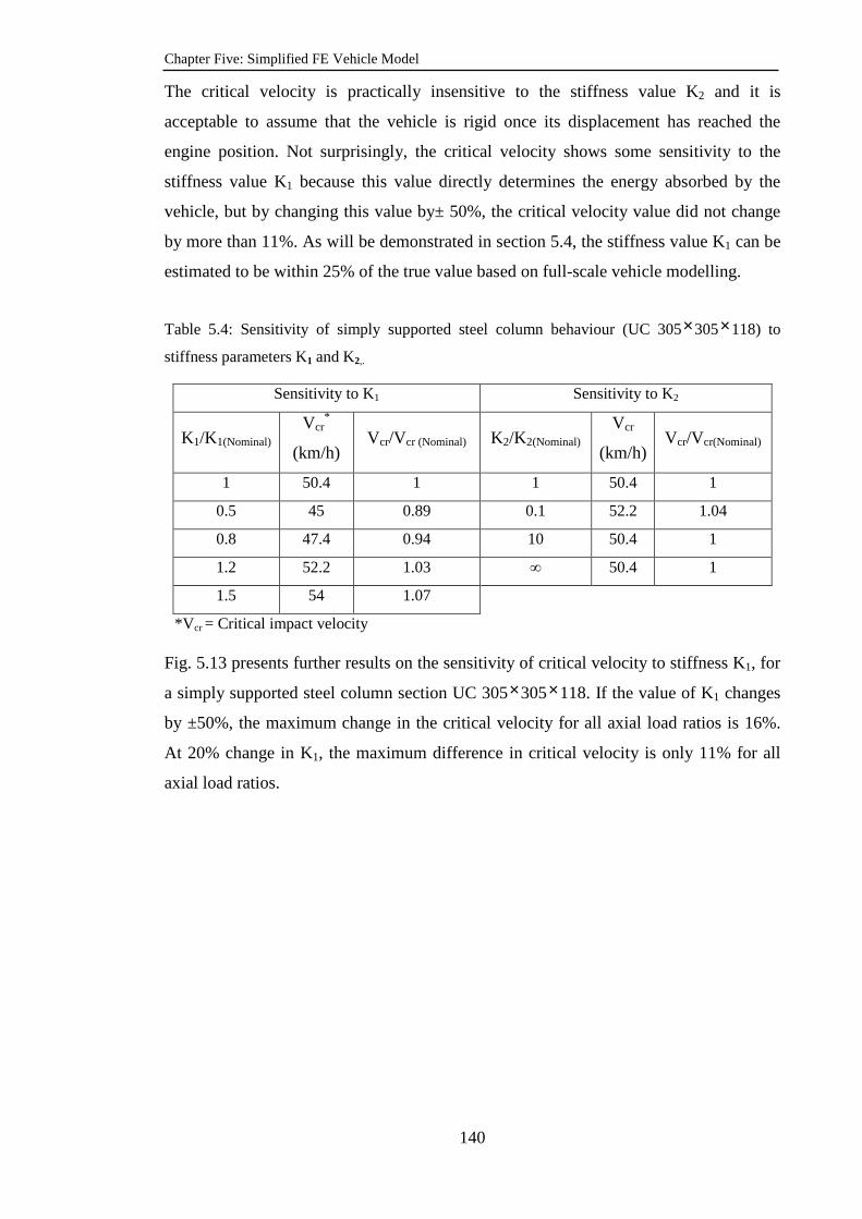
Chapter Five: Simplified FE Vehicle Model
140
The critical velocity is practically insensitive to the stiffness value K2 and it is
acceptable to assume that the vehicle is rigid once its displacement has reached the
engine position. Not surprisingly, the critical velocity shows some sensitivity to the
stiffness value K1 because this value directly determines the energy absorbed by the
vehicle, but by changing this value by± 50%, the critical velocity value did not change
by more than 11%. As will be demonstrated in section 5.4, the stiffness value K1 can be
estimated to be within 25% of the true value based on full-scale vehicle modelling.
Table 5.4: Sensitivity of simply supported steel column behaviour (UC 305×305×118) to
stiffness parameters K1 and K2,.
Sensitivity to K1 Sensitivity to K2
K1/K1(Nominal) Vcr
*
(km/h) Vcr/Vcr (Nominal) K2/K2(Nominal)
Vcr
(km/h) Vcr/Vcr(Nominal)
1 50.4 1 1 50.4 1
0.5 45 0.89 0.1 52.2 1.04
0.8 47.4 0.94 10 50.4 1
1.2 52.2 1.03 ∞ 50.4 1
1.5 54 1.07
*V cr = Critical impact velocity Fig. 5.13 presents further results on the sensitivity of critical velocity to stiffness K1, for
a simply supported steel column section UC 305×305×118. If the value of K1 changes
by ±50%, the maximum change in the critical velocity for all axial load ratios is 16%.
At 20% change in K1, the maximum difference in critical velocity is only 11% for all
axial load ratios.

Chapter Five: Simplified FE Vehicle Model
141
0
0.2
0.4
0.6
0.8
1
1.2
10 34 58 82 106 130Critical impact velocity (km/h)
P/P
Des
ign
Full scale vehicle modelSVM-K1=KSVM-K1=0.5KSVM-K1=0.8KSVM-K1=1.2KSVM-K1=1.5KRigid impactor
Figure 5.13: Comparison of axial load – critical velocity curves between the full scale vehicle
model and the simplified vehicle model using five values of vehicle frontal stiffness (K1) for the
simply supported steel column section UC 305×305×118 subjected to the transverse impact of
a 1994 Chevrolet Pick-up vehicle.
5.3.3. Determining an appropriate simplified vehicle model
Since the vehicle becomes very stiff when its displacement has reached the engine box,
it may be considered acceptable to model the vehicle simply as a rigid impactor. To
assess this claim, an extensive amount of numerical simulations have been performed to
compare the critical impact velocities for a number of columns between the following
four vehicle models:
a) full-scale numerical vehicle model;
b) spring mass system with bilinear vehicle force - displacement relationship and
finite stiffness value K2;
c) bilinear spring force - displacement curve with the same stiffness value K1 as in
(b) but K2 being infinite (rigid);
d) whole vehicle as a rigid impactor throughout.
The simulation results are presented in Figs. 5.14 to 5.18 for the different column
conditions as specified in Table 5.2. In all cases, buckling was about the weak axis
of the column. The results are presented as a column axial load ratio - critical
velocity relationship.
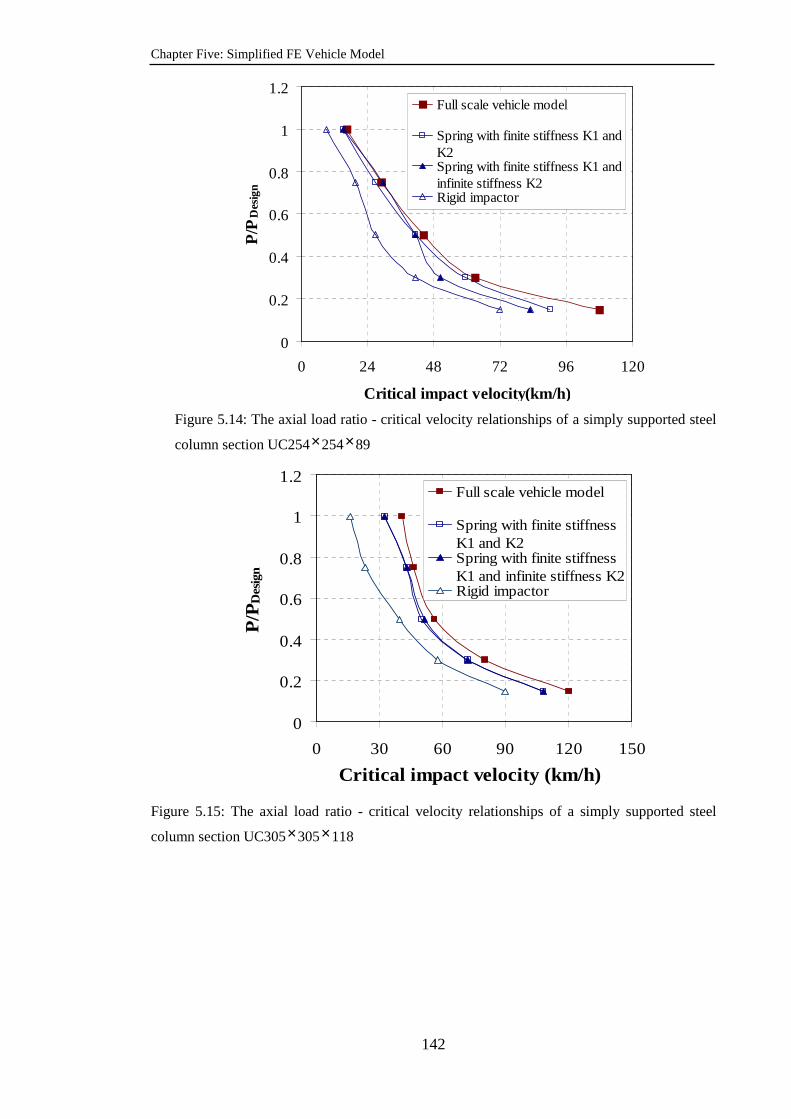
Chapter Five: Simplified FE Vehicle Model
142
0
0.2
0.4
0.6
0.8
1
1.2
0 24 48 72 96 120
Critical impact velocity(km/h)
P/P
Des
ign
Full scale vehicle model
Spring with finite stiffness K1 andK2Spring with finite stiffness K1 andinfinite stiffness K2Rigid impactor
Figure 5.14: The axial load ratio - critical velocity relationships of a simply supported steel
column section UC254×254×89
0
0.2
0.4
0.6
0.8
1
1.2
0 30 60 90 120 150
Critical impact velocity (km/h)
P/P
Des
ign
Full scale vehicle model
Spring with finite stiffnessK1 and K2Spring with finite stiffnessK1 and infinite stiffness K2Rigid impactor
Figure 5.15: The axial load ratio - critical velocity relationships of a simply supported steel
column section UC305×305×118

Chapter Five: Simplified FE Vehicle Model
143
0.4
0.55
0.7
0.85
1
1.15
20 44 68 92 116 140
Critical impact velocity (km/h)
P/P
Des
ign
Full scale FE vehicle model
Spring with finite stiffness K1and K2Spring with finite stiffness K1and infinite stiffness K2Rigid impactor
Figure 5.16: The axial load ratio - critical velocity relationships of a simply supported steel
column section UC356×368×202.
0.2
0.4
0.6
0.8
1
1.2
0 30 60 90 120 150Critical impact velocity(km/h)
P/P
Des
ign
Full scale vehicle model
Spring with finite stiffness K1and K2Spring with finite stiffness K1and infinite stiffness K2Rigid impactor
Figure 5.17: The axial load ratio - critical velocity relationships of a propped cantilever steel
column section UC254×254×89
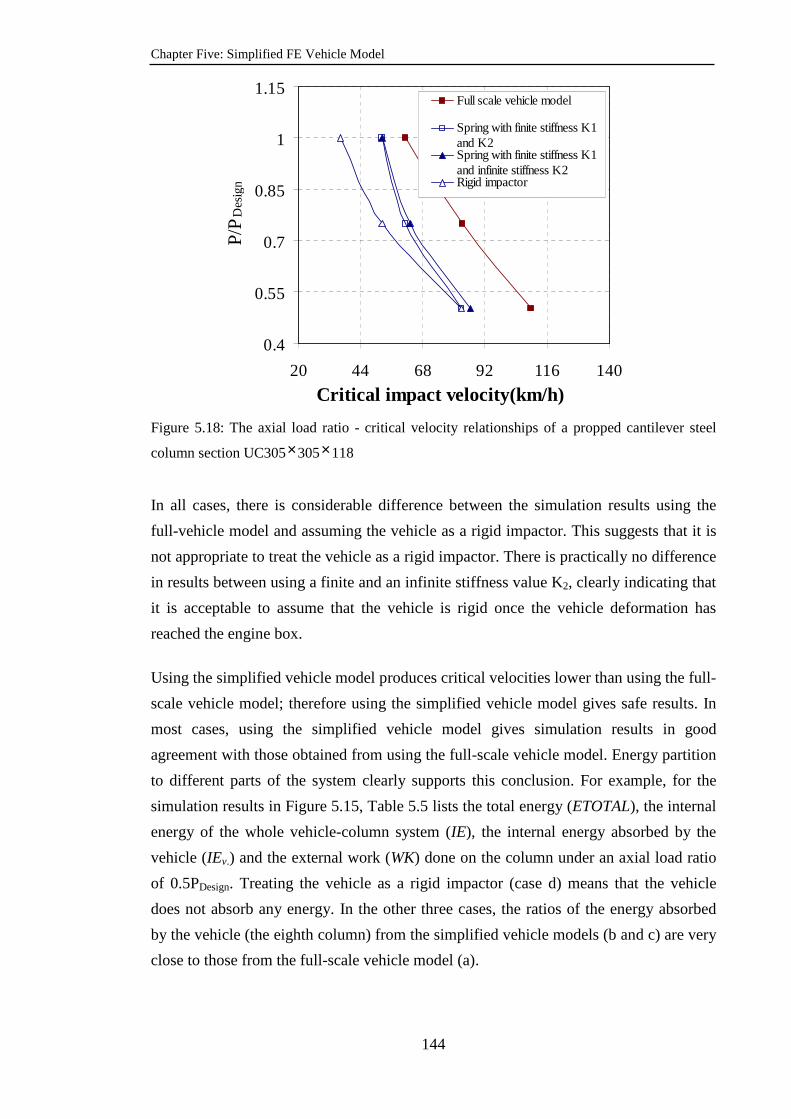
Chapter Five: Simplified FE Vehicle Model
144
0.4
0.55
0.7
0.85
1
1.15
20 44 68 92 116 140
Critical impact velocity(km/h)
P/P
Des
ign
Full scale vehicle model
Spring with finite stiffness K1and K2Spring with finite stiffness K1and infinite stiffness K2Rigid impactor
Figure 5.18: The axial load ratio - critical velocity relationships of a propped cantilever steel
column section UC305×305×118
In all cases, there is considerable difference between the simulation results using the
full-vehicle model and assuming the vehicle as a rigid impactor. This suggests that it is
not appropriate to treat the vehicle as a rigid impactor. There is practically no difference
in results between using a finite and an infinite stiffness value K2, clearly indicating that
it is acceptable to assume that the vehicle is rigid once the vehicle deformation has
reached the engine box.
Using the simplified vehicle model produces critical velocities lower than using the full-
scale vehicle model; therefore using the simplified vehicle model gives safe results. In
most cases, using the simplified vehicle model gives simulation results in good
agreement with those obtained from using the full-scale vehicle model. Energy partition
to different parts of the system clearly supports this conclusion. For example, for the
simulation results in Figure 5.15, Table 5.5 lists the total energy (ETOTAL), the internal
energy of the whole vehicle-column system (IE), the internal energy absorbed by the
vehicle (IEv.) and the external work (WK) done on the column under an axial load ratio
of 0.5PDesign. Treating the vehicle as a rigid impactor (case d) means that the vehicle
does not absorb any energy. In the other three cases, the ratios of the energy absorbed
by the vehicle (the eighth column) from the simplified vehicle models (b and c) are very
close to those from the full-scale vehicle model (a).
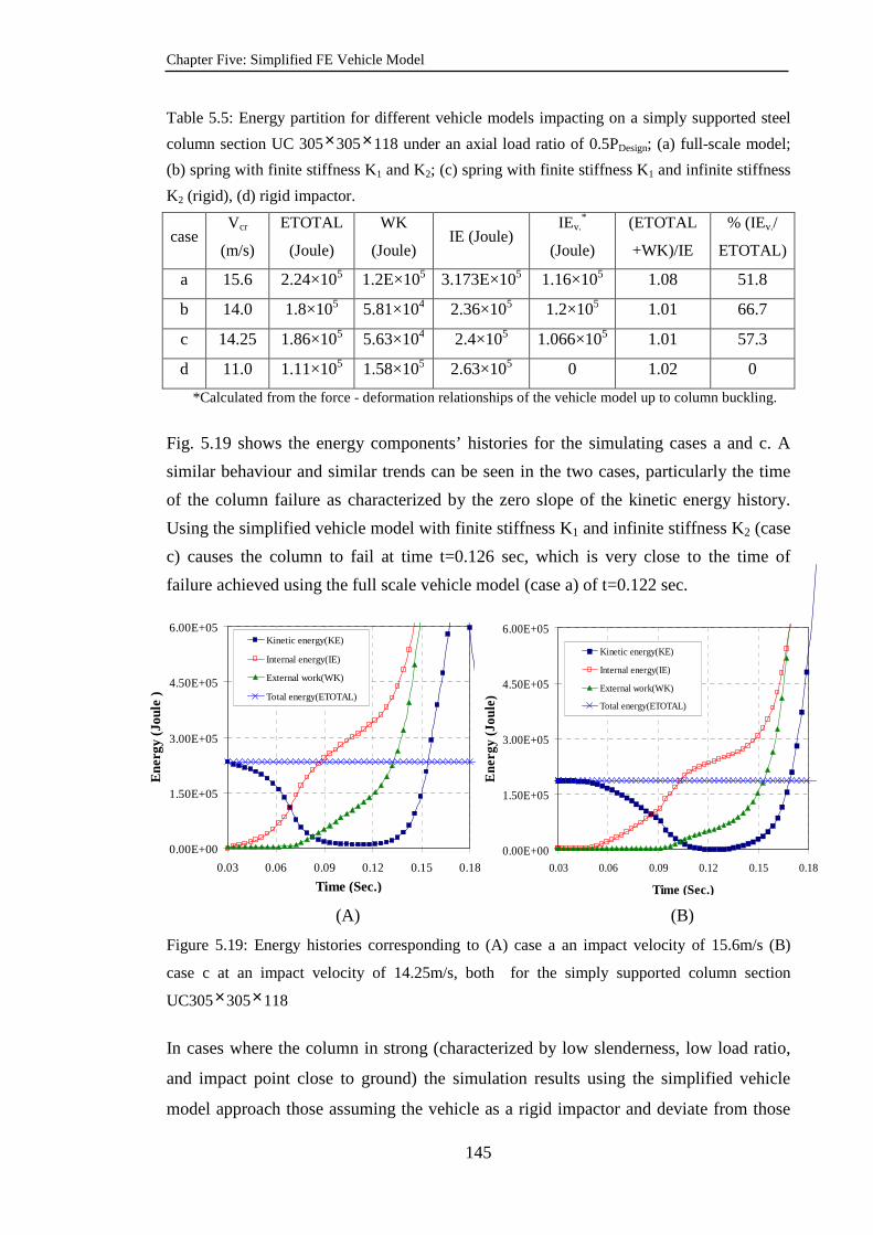
Chapter Five: Simplified FE Vehicle Model
145
Table 5.5: Energy partition for different vehicle models impacting on a simply supported steel
column section UC 305×305×118 under an axial load ratio of 0.5PDesign; (a) full-scale model;
(b) spring with finite stiffness K1 and K2; (c) spring with finite stiffness K1 and infinite stiffness
K2 (rigid), (d) rigid impactor.
case Vcr
(m/s)
ETOTAL
(Joule)
WK
(Joule) IE (Joule)
IEv.*
(Joule)
(ETOTAL
+WK)/IE
% (IEv./
ETOTAL)
a 15.6 2.24×10⁵ 1.2E×105 3.173E×105 1.16×10⁵ 1.08 51.8
b 14.0 1.8×10⁵ 5.81×10⁴ 2.36×10⁵ 1.2×10⁵ 1.01 66.7
c 14.25 1.86×10⁵ 5.63×10⁴ 2.4×10⁵ 1.066×10⁵ 1.01 57.3
d 11.0 1.11×10⁵ 1.58×10⁵ 2.63×10⁵ 0 1.02 0
*Calculated from the force - deformation relationships of the vehicle model up to column buckling.
Fig. 5.19 shows the energy components’ histories for the simulating cases a and c. A
similar behaviour and similar trends can be seen in the two cases, particularly the time
of the column failure as characterized by the zero slope of the kinetic energy history.
Using the simplified vehicle model with finite stiffness K1 and infinite stiffness K2 (case
c) causes the column to fail at time t=0.126 sec, which is very close to the time of
failure achieved using the full scale vehicle model (case a) of t=0.122 sec.
(A) (B)
Figure 5.19: Energy histories corresponding to (A) case a an impact velocity of 15.6m/s (B)
case c at an impact velocity of 14.25m/s, both for the simply supported column section
UC305×305×118
In cases where the column in strong (characterized by low slenderness, low load ratio,
and impact point close to ground) the simulation results using the simplified vehicle
model approach those assuming the vehicle as a rigid impactor and deviate from those
0.00E+00
1.50E+05
3.00E+05
4.50E+05
6.00E+05
0.03 0.06 0.09 0.12 0.15 0.18
Time (Sec.)
Ene
rgy
(Jou
le )
Kinetic energy(KE)
Internal energy(IE)
External work(WK)
Total energy(ETOTAL)
0.00E+00
1.50E+05
3.00E+05
4.50E+05
6.00E+05
0.03 0.06 0.09 0.12 0.15 0.18
Time (Sec.)
Ene
rgy
(Jou
le)
Kinetic energy(KE)
Internal energy(IE)
External work(WK)
Total energy(ETOTAL)
Chapter Five: Simplified FE Vehicle Model
146
when using the full-scale vehicle model. This is because the failure of such columns
requires a large amount of impact energy. When this happens, a large part of the impact
energy is absorbed by deformations of other parts of the full-scale vehicle (such as in
the rear part of the vehicle, shown in Fig.5.22) which are not included in the simplified
vehicle model which is based on deformation in front of the engine box.
5.3.4. Effect of increasing vehicle weight
The proposed simplified vehicle model was obtained for an empty vehicle. To examine
whether the same spring force - displacement relationship can be used when there are
goods in the vehicle, further simulations have been carried out using the same 1994
Chevrolet Pick-up vehicle, but by increasing the weight of the vehicle by 1 tonnes and
1.5 tonnes. Figs. 5.20 and 5.21 compare the simulation results. Compared with Fig.
5.15, the correlation of the simulation results using the simplified vehicle model with
the full-scale vehicle model is slightly worsened. This is caused by increased energy
absorption in other parts of the vehicle that are not included in the simplified vehicle
model. Increasing the vehicle weight increases the tendency for this to happen.
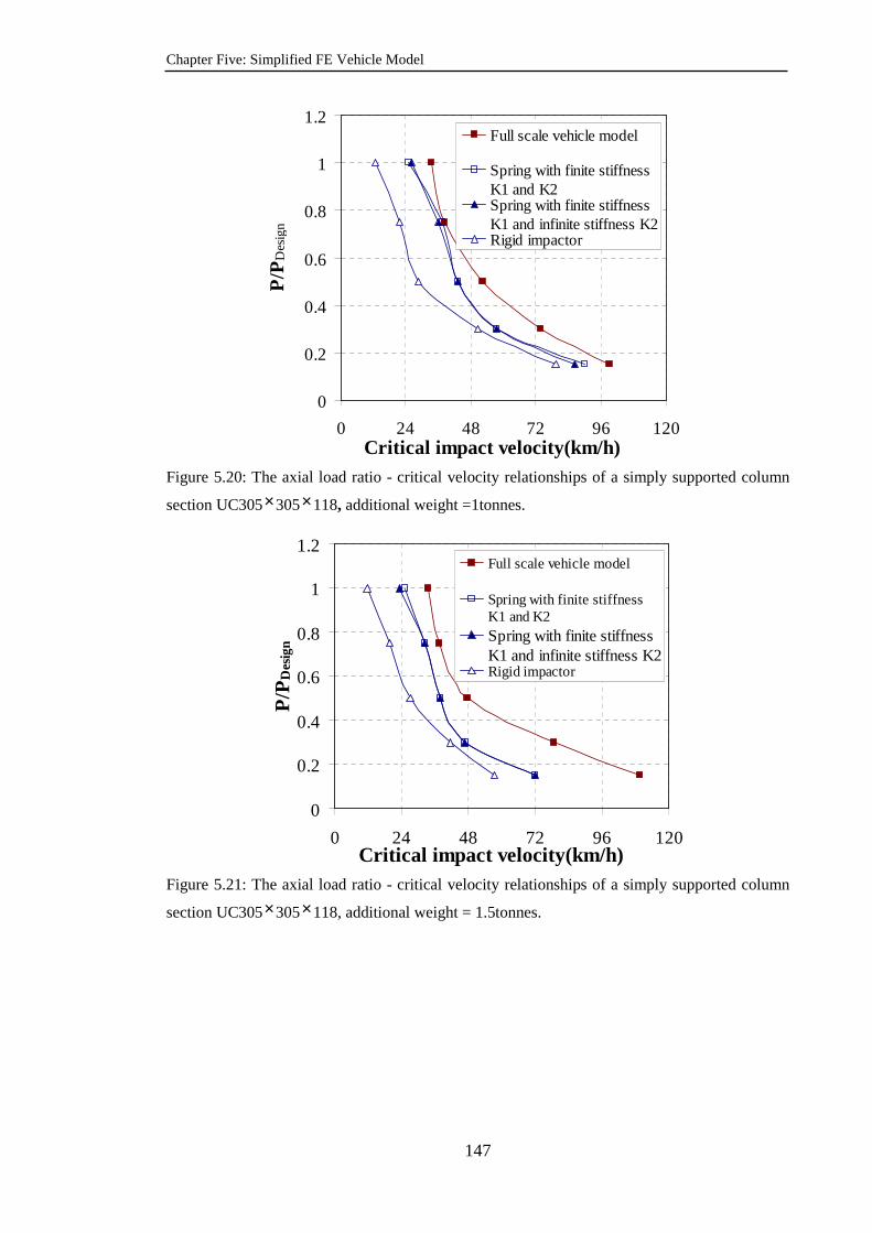
Chapter Five: Simplified FE Vehicle Model
147
0
0.2
0.4
0.6
0.8
1
1.2
0 24 48 72 96 120Critical impact velocity(km/h)
P/P
Des
ign
Full scale vehicle model
Spring with finite stiffnessK1 and K2Spring with finite stiffnessK1 and infinite stiffness K2Rigid impactor
Figure 5.20: The axial load ratio - critical velocity relationships of a simply supported column
section UC305×305×118, additional weight =1tonnes.
0
0.2
0.4
0.6
0.8
1
1.2
0 24 48 72 96 120Critical impact velocity(km/h)
P/P
Des
ign
Full scale vehicle model
Spring with finite stiffnessK1 and K2Spring with finite stiffnessK1 and infinite stiffness K2Rigid impactor
Figure 5.21: The axial load ratio - critical velocity relationships of a simply supported column
section UC305×305×118, additional weight = 1.5tonnes.

Chapter Five: Simplified FE Vehicle Model
148
(a) A simply supported steel column section UC 356×368×202, P=0.3PDesign, V=170km/h.
(b) A propped cantilever steel column section UC 305×305×118, P=0.3PDesign,
V=180km/h
(c) A simply supported steel column section UC 305×305×118, P=0.15PDesign,
V=130km/h, additional weight = 1.5tonnes
Figure 5.22: Deformation shape of the C2500 vehicle after a steel column impact for low axial
load ratios
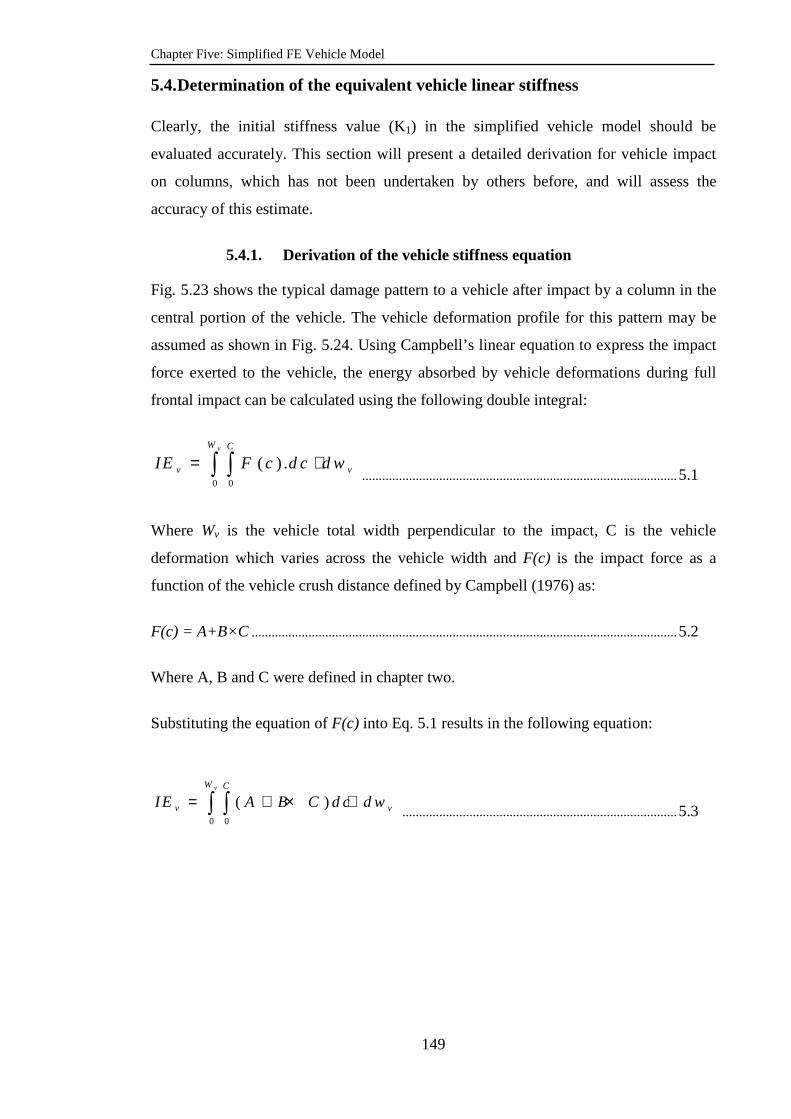
Chapter Five: Simplified FE Vehicle Model
149
5.4. Determination of the equivalent vehicle linear stiffness Clearly, the initial stiffness value (K1) in the simplified vehicle model should be
evaluated accurately. This section will present a detailed derivation for vehicle impact
on columns, which has not been undertaken by others before, and will assess the
accuracy of this estimate.
5.4.1. Derivation of the vehicle stiffness equation
Fig. 5.23 shows the typical damage pattern to a vehicle after impact by a column in the
central portion of the vehicle. The vehicle deformation profile for this pattern may be
assumed as shown in Fig. 5.24. Using Campbell’s linear equation to express the impact
force exerted to the vehicle, the energy absorbed by vehicle deformations during full
frontal impact can be calculated using the following double integral:
0 0
( ) .vW C
v vIE F c d c d w= ⋅∫ ∫ .............................................................................................. 5.1
Where Wv is the vehicle total width perpendicular to the impact, C is the vehicle
deformation which varies across the vehicle width and F(c) is the impact force as a
function of the vehicle crush distance defined by Campbell (1976) as:
F(c) = A+B×C ............................................................................................................................... 5.2
Where A, B and C were defined in chapter two.
Substituting the equation of F(c) into Eq. 5.1 results in the following equation:
0 0
( )vW C
v vIE A B C d c d w= + × ⋅∫ ∫ .................................................................................. 5.3

Chapter Five: Simplified FE Vehicle Model
150
Figure 5.23: Damage profile of the C2500 vehicle after a frontal impact in the central region on a column
Figure 5.24: Simplified damage profile of a vehicle after frontal impact in the central region on
a column
For frontal impact with a column in the middle of the vehicle, see Fig. 5.24 above, the
vehicle displacement can be expressed as follows:
For ( )
02
v cv
W hw
−≤ ≤
m a x
( ) / 2v c v
C C
W h w=
− ............................................................................................................... 5.4
Wv
Cmax
(Wv-hc)/2 (Wv-hc)/2 hc
Cmax
(Wv-hc)/2
wv
C
wv
c

Chapter Five: Simplified FE Vehicle Model
151
m a x2
( )v
v c
C wC
W h
×∴ =− ................................................................................................................ 5.5
For ( ) ( )
2 2v c v c
v
W h W hw
− +≤ ≤
m a xC C=
..................................................................................................................................... 5.6
Where: hc is the width of the column perpendicular to the direction of impact.
By substituting Eqs. 5.5 and 5.6 into Eq. 5.3 to compute the energy absorbed by vehicle
deformations, the following is obtained:
m a x
( )
2
0 0 0
( ) 2 ( )
v cW hC C
v c vIE h A B C d c A B C d c d w
−
= + + + ⋅∫ ∫ ∫ ........................... 5.7
( ) 22 2
m a x
m a x
0
[ ][ ] 2 2
2
v cW h
vv c
B CB C A C d w
IE A C h
−
+= + + ∫ ..................... 5.8
2m a x
m a x
( )2 2m a x m a x2
0
[ ]2
2 21[ ( ) ( ) ]
( ) 2 ( )2
v c
v c
W h
v v vv c v c
B CI E A C h
C CA w B w d w
W h W h
−
= + +
+− −∫
............................. 5.9
2m a x
m a x
( )22 3m a x m a x 2
0
[ ]2
2 212[ ( ) ( ) ]
( ) 2 6 ( )
v c
v c
W hv
vv c v c
B CIE A C h
C w CA B w
W h W h
−
= + +
+− −
............................ 5.10
2m a x 2
m a x m a x m a x
( )[ ] [ ]
2 2 3v c
v c
W hB C BIE A C h A C C
−= + + + ................. 5.11
2m a xm a x
( ) ( 2 )
2 6v c v c
v
W h W hIE A C B C
+ += + ........................................ 5.12
The potential energy of a spring with linear spring stiffness is:
Chapter Five: Simplified FE Vehicle Model
152
21 m a x
1
2vI E K C= ................................................................................................................ 5.13
Equating Eq.5.12 to Eq.5.13 gives:
2m a x m a x
1 2m a x
( ) ( 2 )2 [ ]
2 6v c v cW h W h
A C B CK
C
+ ++= ............................................ 5.14
In Eq. 5.14, Cmax is the maximum displacement of the vehicle in front of the engine box.
5.4.2. Validation of the suggested stiffness equation
There is a lack of data to enable the accuracy of Eq.5.14 to be directly and
comprehensively assessed. As partial validation, the calculation results for the
Chevrolet C2500 Pick-up using Eq.5.14 are compared with the stiffness values obtained
from the numerical simulations reported in section 5.3.1.2 in addition to the stiffness
values obtained from the numerical simulations using two larger virtual column sizes
(500 mm and 750mm).
For this calculation, the values of A and B are A = 52.686kN/m and B = 509.623kN/m2
according Eqs. 2.8 to 2.11 in chapter two. The value of Cmax is 0.625m according to the
full-scale numerical simulation results in section 5.3.1.2 Wv=1.63m. Table 5.6 compares
the calculated and the numerically extracted stiffness results for the different column
dimensions (hc) in contact with the vehicle. The difference between the calculation
results using Eq.5.14 and the numerically extracted results is within 25%. Also
Campbell (Campbell, 1976) indicated that the applicability of Eq. 5.2 should be limited
to hc/Wv > 25%. The results in Table 5.6 for smaller column dimensions (h/Wv = 16%
and 19. 3%) indicate that Eq. 5.2 can be used for a h/Wv ratio lower than 25%.
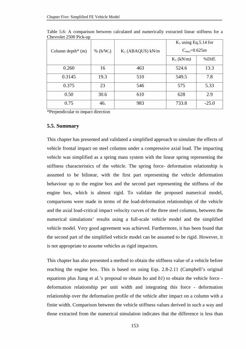
Chapter Five: Simplified FE Vehicle Model
153
Table 5.6: A comparison between calculated and numerically extracted linear stiffness for a Chevrolet 2500 Pick-up
Column depth* (m) % (h/Wv) K1 (ABAQUS) kN/m
K1 using Eq.5.14 for
Cmax=0.625m
K1 (kN/m) %Diff.
0.260 16 463 524.6 13.3
0.3145 19.3 510 549.5 7.8
0.375 23 546 575 5.33
0.50 30.6 610 628 2.9
0.75 46. 983 733.8 -25.0
*Perpendicular to impact direction
5.5. Summary
This chapter has presented and validated a simplified approach to simulate the effects of
vehicle frontal impact on steel columns under a compressive axial load. The impacting
vehicle was simplified as a spring mass system with the linear spring representing the
stiffness characteristics of the vehicle. The spring force- deformation relationship is
assumed to be bilinear, with the first part representing the vehicle deformation
behaviour up to the engine box and the second part representing the stiffness of the
engine box, which is almost rigid. To validate the proposed numerical model,
comparisons were made in terms of the load-deformation relationships of the vehicle
and the axial load-critical impact velocity curves of the three steel columns, between the
numerical simulations’ results using a full-scale vehicle model and the simplified
vehicle model. Very good agreement was achieved. Furthermore, it has been found that
the second part of the simplified vehicle model can be assumed to be rigid. However, it
is not appropriate to assume vehicles as rigid impactors.
This chapter has also presented a method to obtain the stiffness value of a vehicle before
reaching the engine box. This is based on using Eqs. 2.8-2.11 (Campbell’s original
equations plus Jiang et al.’s proposal to obtain bo and b1) to obtain the vehicle force -
deformation relationship per unit width and integrating this force - deformation
relationship over the deformation profile of the vehicle after impact on a column with a
finite width. Comparison between the vehicle stiffness values derived in such a way and
those extracted from the numerical simulation indicates that the difference is less than

Chapter Five: Simplified FE Vehicle Model
154
25% for different column section sizes. Also Campbell’s original condition that the
column width be at least 25% of the vehicle width may be removed.

Chapter Six: The Derivations of a Simplified Analytical Method
155
Chapter Six
The Derivations of a Simplified Analytical Method for Predicting
the Critical Velocity of Transverse Rigid Body Impact and
Vehicle Impact on Steel Columns
6.1. Introduction
This chapter presents the development of a simplified analytical method to predict the
critical velocity of rigid body impact and vehicle impact on steel columns under axial
compressive load. This method is based on the energy balance with a quasi-static
approximation of the column behaviour. This general method has been widely used for
beams under lateral impact without any axial load (Jones, 1995, Wen et al., 1995,
Bambach et al., 2008) but column buckling adds complexity to the problem. For
simplification, the observations and conclusions drawn from the parametric study and
numerical simulations conducted in chapters four and five have been used to provide
guidance on establishing several assumptions.
Although assuming that the impacting mass behaves as a rigid body may give more
conservative design results in terms of the critical impact velocity because all the impact
energy is only absorbed by column deformations, it neglects the amount of impact
energy that could be absorbed by vehicle deformations which may affect the column
behaviour and failure. Moreover, the results presented in chapter five have shown that
vehicle deformations absorb a considerable percentage of the impact energy which can
significantly reduce the kinetic energy imparted to the column. The objective of this
chapter is to present a simple but effective approach to account for vehicle deformations
in the energy balance equation.

Chapter Six: The Derivations of a Simplified Analytical Method
156
6.2. Derivation of the simplified analytical method
It should be pointed out that the main emphasis of this analytical method is to obtain the
column axial load - critical impact velocity relationship. The critical impact velocity is
defined in chapter four as the minimum velocity of the impact body that causes the
column to lose its stability. From reviewing the available literature (chapter two), it can
be concluded that the most simplistic analytical method for structures subjected to
transverse impact load would be to assume a quasi-static behaviour (Jones, 1995, Wen
et al., 1995, Bambach et al., 2008, Shope, 2006). Therefore, the combination of an
energy balance approach with a quasi-static approximation of column behaviour will be
used in the current study to provide a simplified method which is intended to provide an
accurate enough prediction of the critical velocity of a vehicular impact on a steel
column.
The energy balance approach is more appropriate for impact events with a very short
duration compared with the natural period of the whole structural system. This is
because, in such a dynamic event, the impact loading history is unimportant compared
to the total impact energy imparted to the impacted structural member (Jones, 1995).
This approach can be used by either assuming all the impact kinetic energy is absorbed
only by the impacted column which means the impacting object behaves as rigid body
or by assuming that both the impacted column and the impacting object absorb the
kinetic energy of the impact. Both assumptions will be used in this chapter to determine
the critical impact velocity.
6.2.1. Developing the energy balance equation
The general energy balance equation, as employed in ABAQUS/Explicit, is:
IE+VD+KE+FD-WK=ETOTAL=Energy Balance =CONSTANT .................................... 6.1
Where IE is the internal energy (consisting of both the recoverable or elastic strain
energy, SE, and the plastic strain energy, PD), VD the viscous dissipation energy, KE
the residual kinetic energy, FD the frictional dissipation energy at the contact zone, WK
the work done by the external forces, and ETOTAL the total conserved energy of the
system (the energy balance of the system).

Chapter Six: The Derivations of a Simplified Analytical Method
157
For the critical situation, the column and the impactor are at rest, therefore KE=0. As
shown in chapter four, due to the short duration of impact, the viscous dissipation
energy at the critical condition is negligible compared to the initial impact energy even
after introducing a damping effect, making VD=0. Assuming there is no friction under
direct impact, then FD=0.
Hence, Eq. 6.1 becomes:
IE -WK = ETOTAL =Total conserved energy = Total impact energy .............................. 6.2
Or
IE = Total impact energy + WK .................................................................................................. 6.3
For the case of rigid impact, the IE results from the column’s deformations only (i.e.
IE=IEcol), whilst for the flexible vehicle impact, this term also includes the energy
absorbed by vehicle deformation (i.e. IE=IEcol+ IEv.).
The derivation of each term in the above energy balance equation for both rigid impact
and vehicle impact will be presented in the following subsections.
6.2.2. Energy absorbed by the column’s deformation (IEcol)
In the majority of previous theoretical studies which have adopted the energy balance
approach to predict structural behaviour under transverse impact, the material behaviour
was assumed to be rigid-plastic, making SE=0. This assumption would lead to an over
prediction of the structural permanent displacements (Jones, 1995, Samuelides and
Frieze, 1984), particularly if the transverse displacements are small or moderate.
Dorogoy (2008) confirmed this conclusion by undertaking a numerical investigation
into the dynamic impact response of an aluminium beam subjected to transverse impact
with no axial restraint. Moreover, the parametric study results of chapter four on steel
columns under transverse impact indicate that the elastic strain energy of a column at
failure is a considerable portion of the total internal energy of the column. Therefore,
both the elastic and plastic strain energies will be included in the proposed simplified
method.
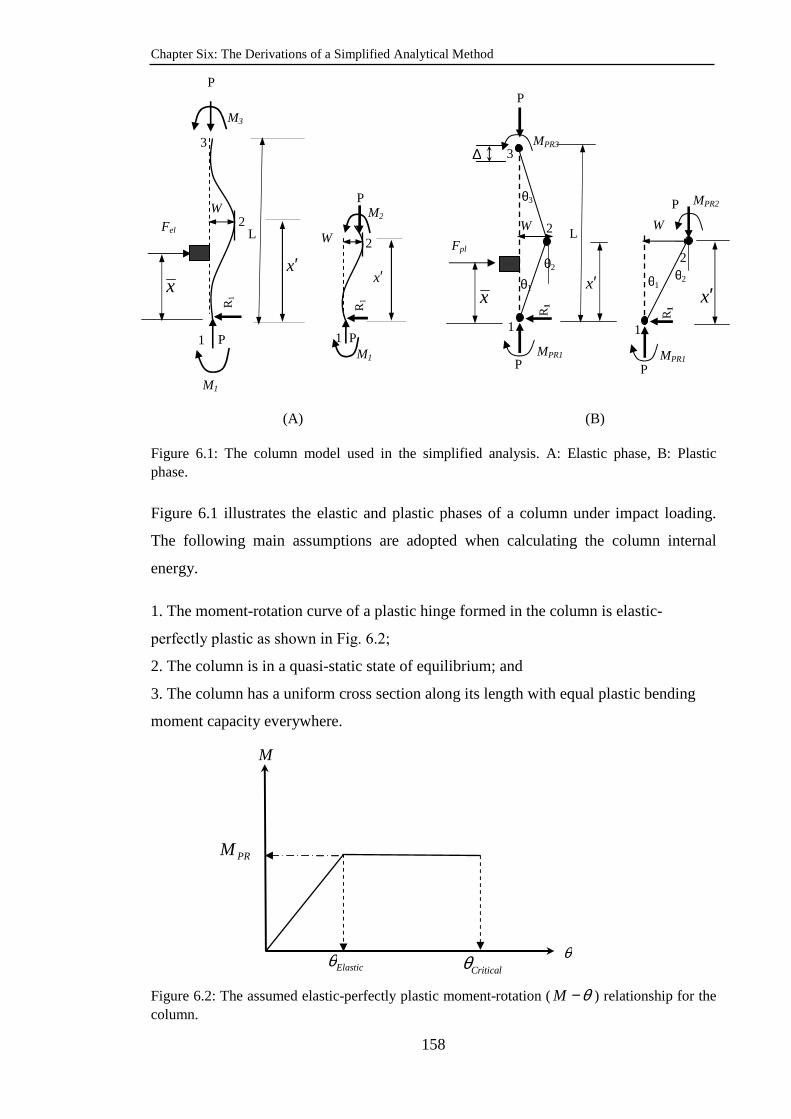
Chapter Six: The Derivations of a Simplified Analytical Method
158
(A) (B)
Figure 6.1: The column model used in the simplified analysis. A: Elastic phase, B: Plastic phase.
Figure 6.1 illustrates the elastic and plastic phases of a column under impact loading.
The following main assumptions are adopted when calculating the column internal
energy.
1. The moment-rotation curve of a plastic hinge formed in the column is elastic-
perfectly plastic as shown in Fig. 6.2;
2. The column is in a quasi-static state of equilibrium; and
3. The column has a uniform cross section along its length with equal plastic bending
moment capacity everywhere.
Figure 6.2: The assumed elastic-perfectly plastic moment-rotation (M θ− ) relationship for the column.
θ2 θ2
M1
x
M1
P
x′
Fel
W
3
2
1
R1
M3
P
L
P
x′
W
2
1
R1
P
M2
x′
Fpl
P
W
∆
L
θ3
θ1
3
2
1
R1
P
x
MPR3
MPR1
x′
P
W
θ1
2
1
R1
MPR1
P
MPR2
PRM
Elasticθ
M
θ Criticalθ
Chapter Six: The Derivations of a Simplified Analytical Method
159
Therefore, the internal energy absorbed by the column can be expressed as:
1
[ ( ) ]2
ni E la s t i c
c o l P R i i C r i t i c a li
IE Mθθ
=
= −∑ ........................................................ 6.4
Where n is the number of plastic hinges required to cause a plastic hinge mechanism in
the column; MPRi is the plastic moment capacity of the column section at the plastic
hinge i, taking into consideration the presence of an axial load; iElasticθ is the maximum
elastic rotation of the column at the plastic hinge i; iCriticalθ is the maximum rotation of
the column at the plastic hinge i
The following section will derive expressions to calculate the rotations iElasticθ and
iCriticalθ .
6.2.2.1. Derivations of the maximum elastic and critical rotations
( iElasticθ and iCriticalθ )
The maximum elastic rotation iElasticθ is calculated based on the column deformation
when the maximum bending moment in the column has just reached the plastic bending
moment capacity. Up to this stage, the column behaviour is assumed to be elastic and
governed by:
xx EIdx
wdM )(
2
2
−= .......................................................................................................................... 6.5
Provided that x PRiM M≤
Where Mx is the elastic bending moment of the column at section (x) along its
longitudinal axis, 2
2
dx
wd is the second derivative of the column deformation w(x) with
respect to the distance x, EI is the flexural stiffness of the column section (E = modulus
of elasticity of the column material, I = 2nd moment of area).
Hence, the maximum elastic rotation iElasticθ is calculated based on the deformations
when the following conditions are reached:

Chapter Six: The Derivations of a Simplified Analytical Method
160
2
2( )x x PR
d wEI M
dx′=− = + for the plastic hinge within the column height; .............. 6.6A
2
0,2( )x x L PR
d wEI M
dx = =− = − for the fix-ended column end ............................................. 6.6 B
Where x′ is the location of the plastic hinge within the column height (see Fig. 6.1).
The above two equations will give two different column deformations. It is proposed to
use the larger deformation to calculate the elastic rotation to ensure that all the plastic
hinges have formed in the cross-section. Because the elastic energy (although
substantial) is still only a minor part of the total strain energy, the above approximation
is acceptable.
Now, referring to Fig. 6.1(B) which represents the deformed shape of the column during
the plastic deformation phase, the maximum or critical plastic rotation iCriticalθ at the
three potential plastic hinge locations can be determined based on the critical or
maximum transverse displacement. The critical displacement will be derived in section
6.2.2.2. It represents the displacement value at which the effect of the bending moment
caused by the axial load becomes just equal to the plastic resistance of the column to
cause global failure of the column.
A. Selecting the elastic deformation shape
To obtain the column deformation using Eq. 6.6 when the maximum bending moment
in the column reaches its plastic bending moment capacity, the deformation shape of the
column should be established first. Previous researchers have suggested using either the
deformation shape of the column under a static load at the position of impact (Biggs,
1964, Humar, 2002) or the buckling mode shape of the column (Sastranegara et al.,
2006, Shope, 2006). For a structural member without any axial load, there is no
considerable difference (Shope, 2006). The numerical simulations presented in chapter
four have revealed that, for columns under moderate to high axial load (>25% column
design load), the static buckling shape is more appropriate.
B. Determination of the intermediate plastic hinge location
The assumed plastic hinge mechanism shown in Fig. 6.1(B) requires the formation of a
plastic hinge between the supports. Without the compressive load, the location of the
intermediate plastic hinge will be at the location of the impacting mass. However, with
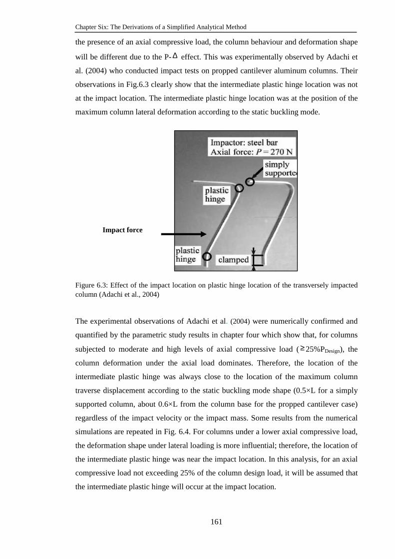
Chapter Six: The Derivations of a Simplified Analytical Method
161
the presence of an axial compressive load, the column behaviour and deformation shape
will be different due to the P-∆ effect. This was experimentally observed by Adachi et
al. (2004) who conducted impact tests on propped cantilever aluminum columns. Their
observations in Fig.6.3 clearly show that the intermediate plastic hinge location was not
at the impact location. The intermediate plastic hinge location was at the position of the
maximum column lateral deformation according to the static buckling mode.
Figure 6.3: Effect of the impact location on plastic hinge location of the transversely impacted column (Adachi et al., 2004)
The experimental observations of Adachi et al. (2004) were numerically confirmed and
quantified by the parametric study results in chapter four which show that, for columns
subjected to moderate and high levels of axial compressive load (≥ 25%PDesign), the
column deformation under the axial load dominates. Therefore, the location of the
intermediate plastic hinge was always close to the location of the maximum column
traverse displacement according to the static buckling mode shape (0.5×L for a simply
supported column, about 0.6×L from the column base for the propped cantilever case)
regardless of the impact velocity or the impact mass. Some results from the numerical
simulations are repeated in Fig. 6.4. For columns under a lower axial compressive load,
the deformation shape under lateral loading is more influential; therefore, the location of
the intermediate plastic hinge was near the impact location. In this analysis, for an axial
compressive load not exceeding 25% of the column design load, it will be assumed that
the intermediate plastic hinge will occur at the impact location.
Impact force
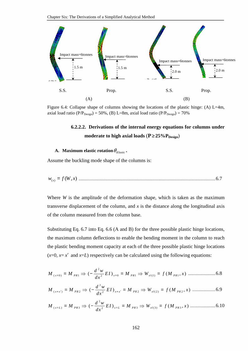
Chapter Six: The Derivations of a Simplified Analytical Method
162
S.S. Prop. S.S. Prop.
(A) (B)
Figure 6.4: Collapse shape of columns showing the locations of the plastic hinge: (A) L=4m, axial load ratio (P/PDesign) = 50%, (B) L=8m, axial load ratio (P/PDesign) = 70%
6.2.2.2. Derivations of the internal energy equations for columns under
moderate to high axial loads (P≥ 25%PDesign)
A. Maximum elastic rotation iElasticθ .
Assume the buckling mode shape of the columns is:
),()( xWfw x = .................................................................................................................................. 6.7
Where W is the amplitude of the deformation shape, which is taken as the maximum
transverse displacement of the column, and x is the distance along the longitudinal axis
of the column measured from the column base.
Substituting Eq. 6.7 into Eq. 6.6 (A and B) for the three possible plastic hinge locations,
the maximum column deflections to enable the bending moment in the column to reach
the plastic bending moment capacity at each of the three possible plastic hinge locations
(x=0, x= x′ and x=L) respectively can be calculated using the following equations:
2
( 0 ) 1 0 1 (1) 12( ) ( , )x PR x PR el PR
d wM M EI M W f M x
dx= == ⇒ − = ⇒ = .......................... 6.8
2
( ) 2 2 ( 2 ) 22( ) ( , )x x PR x x PR el PR
d wM M EI M W f M x
dx′ ′= == ⇒ − = ⇒ = ...................... 6.9
2
( ) 3 3 (3 ) 32( ) ( , )x L PR x L PR el PR
d wM M EI M W f M x
dx= == ⇒ − = ⇒ = ........................ 6.10
1.5 m
Impact mass=6tonnes
1.5 m
Impact mass=6tonnes
2.0 m
Impact mass=6tonnes
2.0 m
Impact mass=6tonnes

Chapter Six: The Derivations of a Simplified Analytical Method
163
As explained previously (section 6.2.2.1), the maximum value of the above three
deflections should be used to determine the maximum elastic rotation at the end of the
elastic deformation phase. However, as will be demonstrated by the example below, the
three elastic deformations above converge to one single value.
Once the value of Wel is determined, the maximum elastic rotation can be determined
based on the plastic deformation shape in Fig. 6.1 (B), giving
x
Wel
elasticx ′== )0(θ ;
)()( xLx
WL el
elasticxx ′−′×
=′=θ ; )()( xL
Wel
elasticLx ′−==θ ........................................ 6.11
B. Critical rotation iCriticalθ .
The derivation that follows is adopted from Shope (Shope, 2006) who applied the
procedure to columns subjected to blast loads. Replace the impact by a nominal static
force Fpl. Referring to the left part of Fig. 6.1(B), the reaction of the column at end 1,
(R1) can be determined by assuming a quasi-static equilibrium condition and taking
moment about end 2:
1 31
( )pl PR PRF L x M MR
L
× − − += ................................................................................................. 6.12
Where x is the position of the impact load application measured from the column base.
Now, referring to the right part of Fig. 6.1(B), the relationship between the equivalent
quasi-static transverse force at the impact location (Fpl), the axial compressive load P
and the maximum transverse displacement W can be determined by the moment
equilibrium condition of that part:
When xx ′≥
1 1 2 0PR PRR x M M P W′× + − + × = ............................................................................................... 6.13
And when xx ′<
1 1 2 ( ) 0PR PR plR x M M P W F x x′ ′× + − + × − × − = ................................................................... 6.14
Substituting the value of R1 from Eq. 6.12 into Eqs. 6.13 and 6.14 and solving for Fpl
gives the following equations:

Chapter Six: The Derivations of a Simplified Analytical Method
164
For xx ′≥
31 2( ( 1) )
( )
PRPR PR
pl
MxM M x P W L
L LFL x x
′ ′− + − − ×∴ =
′− ................................................................ 6.15
For xx ′<
31 2( ( 1) )
( )
PRPR PR
pl
MxM M x P W L
L LFL x x
′ ′− + − − ×=
′− .................................................................. 6.16
Fig. 6.5 illustrates the decreasing relationship between the equivalent quasi-static
transverse force Fpl with increasing the transverse displacement W according to Eqs.
6.15 or 6.16. This figure shows that the maximum displacement at which collapse
occurs due to the combined effect of plastic mechanism and axial compressive force
( .crW ) can be determined by equating the equivalent plastic quasi-static force in Eqs.
6.15 or 6.16 to zero and solving for .crW as in Eq. 6.17:
Figure 6.5: Fpl-W relationship
31 2( 1) PR
PR PR
cr
MxM M x
L LWP
′ ′− + −= .......................................................................................... 6.17
Hence, the plastic critical rotations are:
x
Wcr
Criticalx ′== )0(θ ;
)()( xLx
WL cr
Criticalxx ′−′×
=′=θ , ,)()( xL
Wcr
CriticalLx ′−==θ ................................ 6.18
It should be pointed out that since Eq. 6.18 does not contain any reference to the
deformation capacity of the material (ultimate strain), it is only applicable to columns
Wcr Wel
( )elpl W WF =
F
W

Chapter Six: The Derivations of a Simplified Analytical Method
165
where global buckling governs. The numerical results in chapter four indicate that
column global buckling was indeed the governing failure model.
Substituting the values of elastic rotations (Eq. 6.11) and of critical rotations (Eq. 6.18)
into Eq. 6.4, the general expression for the internal energy of the column is obtained as:
)2/()(
1
)2/()(
)2/(1
3
21
elcrPR
elcrPRelcrPRcol
WWMxL
WWMxLx
LWWM
xIE
−′−
+
−′−′
+−′
=
.. 6.19
The following example illustrates the application of the above mentioned procedure to
calculate the internal energy of a propped cantilever steel column.
Example of how to determine the internal energy equation of a propped cantilever
column
1. Elastic rotation iElasticθ
The equation for the elastic buckling shape of a propped cantilever column can be
expressed as (Timoshenko, 1961, Shope, 2006):
( ) sin( ) . cos( ) . (1 )6.2824x
W xw x L x L
Lφ φ φ φ = × − + −
............................................................. 6.20
Where 1.4318
L
πφ = ......................................................................................................................... 6.21
From Eq. 6.6:
2 3
( ) sin( ) cos( )6.2824x PRi
WM EI x L x Mφ φ φ φ−
= × × − + = .................................................... 6.22
According to Eq. 6.20, the location of the maximum transverse displacement is
(x≈ 0.6L). Substituting this value into Eq. 6.22 gives the following equations:
2
( 0) 12
1.4676x PR
EIM W M
L
π= = − × = Giving: (1) 2
2
( )
1.4676PR
el
MW
EI
L
π−=
−, or (1) 0.7
PRel
cr
MW
P≈
Chapter Six: The Derivations of a Simplified Analytical Method
166
And 2
( 0.6 ) 22
1.466x L PR
EIM W M
L
π= = × = Giving: (2) 2
2
1.466PR
el
MW
EI
L
π= , or (2) 0.7
PRel
cr
MW
P≈
Where Pcr is the Euler buckling load of the propped cantilever column defined by:
2
2
2.046cr
EIP
L
π≈
2. Critical rotation iCriticalθ
Substituting x′ =0.6L and MPR1=−MPR, MPR2=MPR and MPR3=0 into Eq. 6.17 for this
column boundary condition (Fig. 6.1(B), assumption 3) gives:
1.4 PR
cr
MW
P=
3. Internal Energy Substituting the values ofx′ , Wcr ,Wel and the corresponding values of MPR1 , MPR2 and
MPR3 into Eq. 6.19 gives:
1 .4 (1 .4
( ) ( )0 .6 2 0 .7 0 .2 4 2 0 .7
P R P R P R P R P R P Rc o l
c r c r
M M M M M MIE
L P P L P P
−= − + × −× ×
2 22.334 5.8341 1 1 1
( ) ( )2. 2
PR PRcol
cr cr
M MIE
L P P L P P
−= − + −
2 2
2
8.16634 41 1 1 1[ ] [ ]
2 (0.7) 2PR PR
colcr cr
M MIE
L P P L P P= − ≈ −
Following the same procedure, the internal energy for the two other boundary conditions
(simple supports at both ends, fixed supports at both ends) have been calculated. Table
6.1 summarizes the results.

Chapter Six: The Derivations of a Simplified Analytical Method
167
Table 6.1: Internal energy equation of the steel column for three boundary conditions
Column
boundary
condition
Mode shape equation (Timoshenko, 1961, Shope, 2006) Internal energy
equation ( colIE )
S-S )sin()( L
xWw x
π×=
)2
11(
4 2
cr
PR
PPL
M −
F-F
−×= )2
cos(12)( L
xWw x
π
2
2
4 1 1( )
(0.5) 2PR
cr
M
L P P−
H-F ( ) sin( ) . cos( ) . (1 )6.2824x
W xw x L x L
Lφ φ φ φ = × − + −
2
2
4 1 1( )
(0.7) 2PR
cr
M
L P P−
S-S: Simple supports, F-F: Fixed-fixed supports, H-F: Hinged or pinned-fixed supports
By observing the above three equations in Table 6.1, a general equation can be written
to express the internal energy of the steel column as follows:
2
2
4 1 1( )
2PR
colcr
MIE
k L P P= − ............................................................................................................ 6.23
Where Pcr and k are the Euler buckling load and the effective length factor of the column
respectively.
6.2.2.3. Derivations for the internal energy equation for columns under
low axial load levels (P< 25%PDesign)
Apart from changing the plastic hinge location, the numerical simulation results of
chapter four also indicate that, for low levels of axial compressive force, the elastic
strain energy absorbed by the impacted steel column is very low compared to the plastic
dissipation energy as exemplified by Fig. 6.6. Therefore, the elastic strain energy will be
excluded from the energy balance equation (i.e. 0ielasticθ = ).
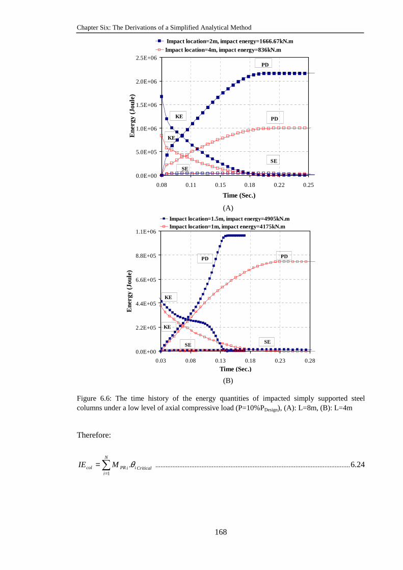
Chapter Six: The Derivations of a Simplified Analytical Method
168
0.0E+00
5.0E+05
1.0E+06
1.5E+06
2.0E+06
2.5E+06
0.08 0.11 0.15 0.18 0.22 0.25
Time (Sec.)
Ene
rgy
(Jou
le)
Impact location=2m, impact energy=1666.67kN.mImpact location=4m, impact energy=836kN.m
PD
KE
SE
PD
KE
SE
(A)
0.0E+00
2.2E+05
4.4E+05
6.6E+05
8.8E+05
1.1E+06
0.03 0.08 0.13 0.18 0.23 0.28
Time (Sec.)
Ene
rgy
(Jou
le)
Impact location=1.5m, impact energy=4905kN.m Impact location=1m, impact energy=4175kN.m
PD
KE
SE
PD
KE
SE
(B)
Figure 6.6: The time history of the energy quantities of impacted simply supported steel columns under a low level of axial compressive load (P=10%PDesign), (A): L=8m, (B): L=4m
Therefore:
∑=
=N
iCriticaliiPRcol MIE
1
.θ .................................................................................................................. 6.24
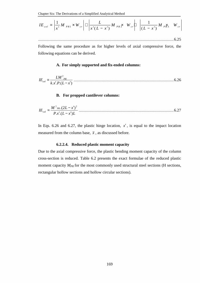
Chapter Six: The Derivations of a Simplified Analytical Method
169
1 2 3
1 1
( ) ( )co l P R cr P R cr P R cr
LIE M W M W M W
x x L x L x= × + × + ×
′ ′ ′ ′− −
................................................................................................................................................................ 6.25
Following the same procedure as for higher levels of axial compressive force, the
following equations can be derived.
A. For simply supported and fix-ended columns:
2
. . .( )PR
col
LMIE
k x P L x=
′ ′− ...................................................................................................................... 6.26
B. For propped cantilever columns:
LxLxP
xLMIE
PR
col ).(.
)2.( 22
′−′′−≈ ................................................................................................................ 6.27
In Eqs. 6.26 and 6.27, the plastic hinge location, x′ , is equal to the impact location
measured from the column base, x , as discussed before.
6.2.2.4. Reduced plastic moment capacity
Due to the axial compressive force, the plastic bending moment capacity of the column
cross-section is reduced. Table 6.2 presents the exact formulae of the reduced plastic
moment capacity MPR for the most commonly used structural steel sections (H sections,
rectangular hollow sections and hollow circular sections).
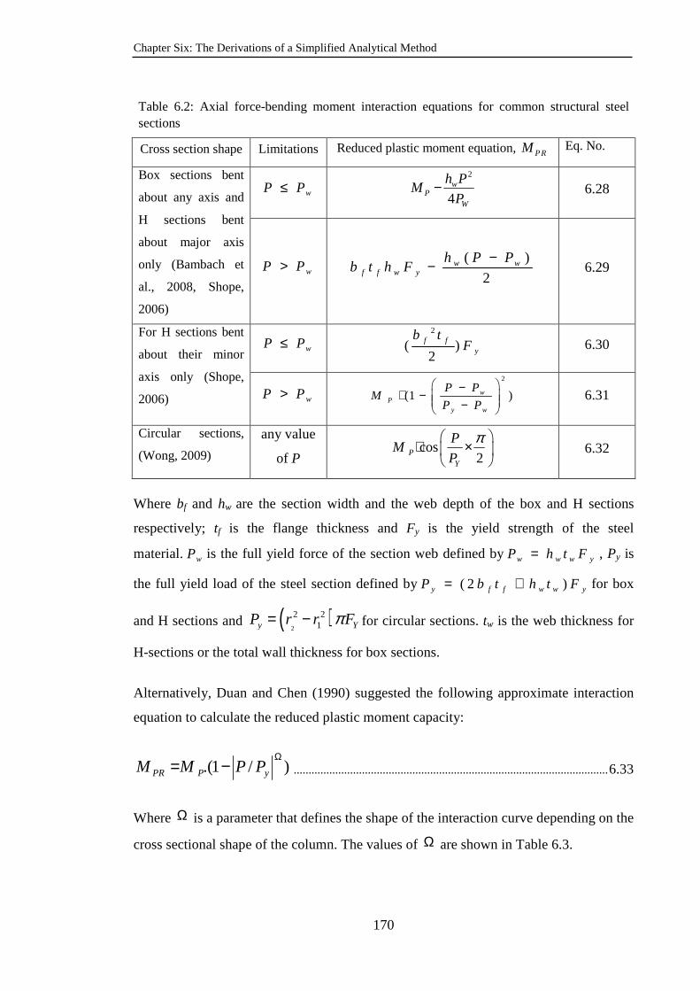
Chapter Six: The Derivations of a Simplified Analytical Method
170
Table 6.2: Axial force-bending moment interaction equations for common structural steel sections
Cross section shape Limitations Reduced plastic moment equation, PRM Eq. No.
Box sections bent
about any axis and
H sections bent
about major axis
only (Bambach et
al., 2008, Shope,
2006)
wPP ≤ W
wP P
PhM
4
2
− 6.28
wPP > ( )
2w w
f f w y
h P Pb t h F
−− 6.29
For H sections bent
about their minor
axis only (Shope,
2006)
wPP ≤ 2
( )2
f fy
b tF 6.30
wPP > 2
(1 )wP
y w
P PM
P P
−⋅ − −
6.31
Circular sections,
(Wong, 2009)
any value
of P cos
2PY
PM
P
π ⋅ ×
6.32
Where bf and hw are the section width and the web depth of the box and H sections
respectively; tf is the flange thickness and Fy is the yield strength of the steel
material. wP is the full yield force of the section web defined by ywww FthP = , Py is
the full yield load of the steel section defined by ywwffy FthtbP )2( += for box
and H sections and ( )2
2 21y YP r r Fπ= − for circular sections. tw is the web thickness for
H-sections or the total wall thickness for box sections.
Alternatively, Duan and Chen (1990) suggested the following approximate interaction
equation to calculate the reduced plastic moment capacity:
)/1.(Ω
−= yPPR PPMM .......................................................................................................... 6.33
Where Ω is a parameter that defines the shape of the interaction curve depending on the
cross sectional shape of the column. The values of Ω are shown in Table 6.3.
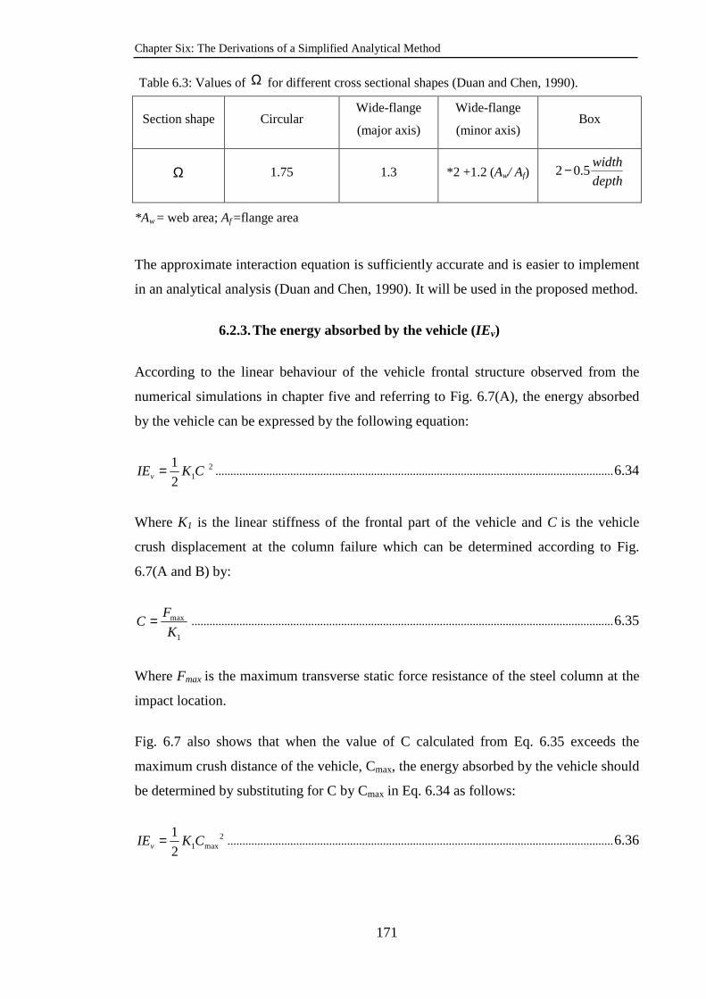
Chapter Six: The Derivations of a Simplified Analytical Method
171
Table 6.3: Values of Ω for different cross sectional shapes (Duan and Chen, 1990).
Section shape Circular Wide-flange
(major axis)
Wide-flange
(minor axis) Box
Ω 1.75 1.3 *2 +1.2 (Aw/ Af) depth
width5.02−
*Aw = web area; Af =flange area
The approximate interaction equation is sufficiently accurate and is easier to implement
in an analytical analysis (Duan and Chen, 1990). It will be used in the proposed method.
6.2.3. The energy absorbed by the vehicle (IEv)
According to the linear behaviour of the vehicle frontal structure observed from the
numerical simulations in chapter five and referring to Fig. 6.7(A), the energy absorbed
by the vehicle can be expressed by the following equation:
2
1
1
2vIE K C= ..................................................................................................................................... 6.34
Where K1 is the linear stiffness of the frontal part of the vehicle and C is the vehicle
crush displacement at the column failure which can be determined according to Fig.
6.7(A and B) by:
max
1
FC
K= ............................................................................................................................................. 6.35
Where Fmax is the maximum transverse static force resistance of the steel column at the
impact location.
Fig. 6.7 also shows that when the value of C calculated from Eq. 6.35 exceeds the
maximum crush distance of the vehicle, Cmax, the energy absorbed by the vehicle should
be determined by substituting for C by Cmax in Eq. 6.34 as follows:
2
1 max
1
2vIE K C= ................................................................................................................................. 6.36
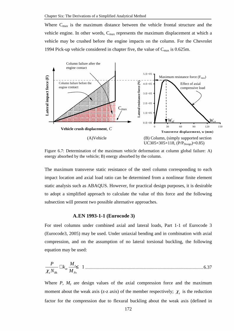
Chapter Six: The Derivations of a Simplified Analytical Method
172
Where Cmax is the maximum distance between the vehicle frontal structure and the
vehicle engine. In other words, Cmax represents the maximum displacement at which a
vehicle may be crushed before the engine impacts on the column. For the Chevrolet
1994 Pick-up vehicle considered in chapter five, the value of Cmax is 0.625m.
(A)Vehicle (B) Column, (simply supported section
UC305×305×118, (P/PDesign)=0.85)
Figure 6.7: Determination of the maximum vehicle deformation at column global failure: A) energy absorbed by the vehicle; B) energy absorbed by the column.
The maximum transverse static resistance of the steel column corresponding to each
impact location and axial load ratio can be determined from a nonlinear finite element
static analysis such as ABAQUS. However, for practical design purposes, it is desirable
to adopt a simplified approach to calculate the value of this force and the following
subsection will present two possible alternative approaches.
A. EN 1993-1-1 (Eurocode 3)
For steel columns under combined axial and lateral loads, Part 1-1 of Eurocode 3
(Eurocode3, 2005) may be used. Under uniaxial bending and in combination with axial
compression, and on the assumption of no lateral torsional buckling, the following
equation may be used:
1zzz
z Rk Pz
MPk
N Mχ+ ≤ ....................................................................................................................... 6.37
Where P, Mz are design values of the axial compression force and the maximum
moment about the weak axis (z-z axis) of the member respectively; zχ is the reduction
factor for the compression due to flexural buckling about the weak axis (defined in
0.E+00
1.E+05
2.E+05
3.E+05
4.E+05
5.E+05
0 30 60 90 120 150
Transverse displacement, w (mm)
Late
ral r
esis
tan
ce fo
rce
(N)
Maximum resistance force (Fmax)
Effect of axial compressive load
Wcr Wel
Column failure before the engine contact
Column failure after the engine contact
Late
ral i
mpa
ct fo
rce
(F)
Vehicle crush displacement, C
Cmax
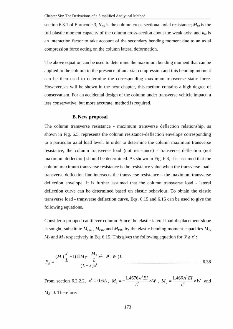
Chapter Six: The Derivations of a Simplified Analytical Method
173
section 6.3.1 of Eurocode 3, NRk is the column cross-sectional axial resistance; Mpz is the
full plastic moment capacity of the column cross-section about the weak axis; and kzz is
an interaction factor to take account of the secondary bending moment due to an axial
compression force acting on the column lateral deformation.
The above equation can be used to determine the maximum bending moment that can be
applied to the column in the presence of an axial compression and this bending moment
can be then used to determine the corresponding maximum transverse static force.
However, as will be shown in the next chapter, this method contains a high degree of
conservatism. For an accidental design of the column under transverse vehicle impact, a
less conservative, but more accurate, method is required.
B. New proposal
The column transverse resistance - maximum transverse deflection relationship, as
shown in Fig. 6.5, represents the column resistance-deflection envelope corresponding
to a particular axial load level. In order to determine the column maximum transverse
resistance, the column transverse load (not resistance) - transverse deflection (not
maximum deflection) should be determined. As shown in Fig. 6.8, it is assumed that the
column maximum transverse resistance is the resistance value when the transverse load-
transverse deflection line intersects the transverse resistance – the maximum transverse
deflection envelope. It is further assumed that the column transverse load - lateral
deflection curve can be determined based on elastic behaviour. To obtain the elastic
transverse load - transverse deflection curve, Eqs. 6.15 and 6.16 can be used to give the
following equations.
Consider a propped cantilever column. Since the elastic lateral load-displacement slope
is sought, substitute MPR1, MPR2 and MPR3 by the elastic bending moment capacities M1,
M2 and M3 respectively in Eq. 6.15. This gives the following equation for x x′≥ :
31 2( ( 1) )
( )el
MxM M x P W L
L LFL x x
′ ′− + − − ×=
′− ............................................................................... 6.38
From section 6.2.2.2, 0.6x L′ = , 2
1 2
1.4676 EIM W
L
π= − × , 2
2 2
1.466 EIM W
L
π= × and
M3=0. Therefore:

Chapter Six: The Derivations of a Simplified Analytical Method
174
2 2
2 2
1.4676 0.6 1.466( ( 1) )
( )el
EI L EIW W P W L
L L LFL x x
π π− × − + × − ×=
′−
2
2
2.0528( )
( )el
EIW P W L
LFL x x
π × − ×∴ =
′− ........................................................................................ 6.39
Similarly, for xx ′≤ :
2
2
2.0528( )
( )pl
EIW P W L
LFL x x
π × − ×∴ =
′− ........................................................................................ 6.40
Going through the same procedure, equations have been derived for simply supported
and fix-ended boundary conditions and the results are given in Table 6.4.
Table 6.4: Elastic transverse load – the transverse deflection equations of the steel column for three types of boundary condition
Column
boundary
condition
Load-deflection equations
For x x′≥
For xx ′≤
S-S 2
2( )
( )el
EIW P W L
LFL x x
π × − ×=
′−
2
2( )
( )el
EIW P W L
LFL x x
π × − ×=
′−
F-F 2
2
4( )
( )el
EIW P W L
LFL x x
π × − ×=
′−
2
2
4( )
( )el
EIW P W L
LFL x x
π × − ×=
′−
H-F 2
2
2.0528( )
( )el
EIW P W L
LFL x x
π × − ×=
′−
2
2
2.0528( )
( )el
EIW P W L
LFL x x
π × − ×=
′−
The above three equations can be represented by a general expression to relate the
transverse force (F) with the transverse deflection (W), as follows:
For x x′≥
2
2 2( )
( )
EIP W L
k LFL x x
π − ×=
′− .................................................................................................................... 6.41
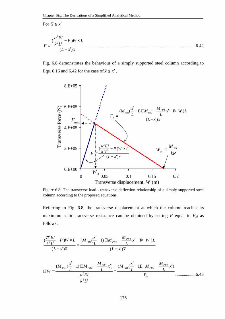
Chapter Six: The Derivations of a Simplified Analytical Method
175
For xx ′≤
2
2 2( )
( )
EIP W L
k LFL x x
π − ×=
′− .................................................................................................................... 6.42
Fig. 6.8 demonstrates the behaviour of a simply supported steel column according to
Eqs. 6.16 and 6.42 for the case of xx ′≤ .
Figure 6.8: The transverse load - transverse deflection relationship of a simply supported steel column according to the proposed equations.
Referring to Fig. 6.8, the transverse displacement at which the column reaches its
maximum static transverse resistance can be obtained by setting F equal to Fpl as
follows:
2
31 22 2( ) ( ( 1) )
( ) ( )
PRPR PR
EI MxP W L M M x P W L
k L L LL x x L x x
π ′ ′− × − + − − ×=
′ ′− −
3 31 2 1 2
2
2 2
( ( 1) ) ( ( 1) )PR PRPR PR PR PR
cr
M Mx xM M x M M x
L L L LWEI P
k L
π
′ ′′ ′− + − − + −∴ = =
..................... 6.43
0.E+00
2.E+05
4.E+05
6.E+05
8.E+05
0 0.05 0.1 0.15 0.2Transverse displacement, W (m)
Tra
nsv
erse
forc
e (N
)
2
2 2( )
( )
EIP W L
k LFL x x
π − ×=
′−
31 2( ( 1) )
( )
PRPR PR
pl
MxM M x P W L
L LFL x x
′ ′− + − − ×=
′−
maxF
kP
MW PR
cr =
elW
Chapter Six: The Derivations of a Simplified Analytical Method
176
Substituting Eq. 6.43 into the general elastic transverse force equations (Eqs. 6.41 and
6.42) or the plastic resistance equations (Eq. 6.15 and Eq. 6.16), the following equations
can be obtained to calculate the column maximum transverse resistance:
For xx ′≥
31 2
max
( ( 1) )(1 )
( )
PRPR PR
cr
M PxM M x L
L L PF
L x x
′ ′− + − −=
′−.................................................................... 6.44
For xx ′≤
31 2
max
( ( 1) )(1 )
( )
PRPR PR
cr
M PxM M x L
L L PF
L x x
′ ′− + − −=
′−.................................................................... 6.45
Eq. 6.45 is more appropriate in the present study since the impact location (x ) is always
lower than or equal to the plastic hinge location (x′ ) as observed from numerical
simulations presented in chapter four.
6.2.4. Derivations of the external work equation
The external work done by the axial compressive force can be calculated by multiplying
the value of the axial compressive load by the axial shortening of the column as follows:
∆×= PWK .............................................................................................................................. 6.46
Where ∆ is the axial shortening of the column.
Referring to Fig. 6.1(B), the axial movement of the column can be calculated from the
following equation:
dxL
axial∫ ×=∆0
ε ........................................................................................................................ 6.47
Where axialε is the axial strain of the column caused by membrane action defined by
continuum mechanics (Wen et al., 1995, Bambach et al., 2008) as:
2
2
1
∂∂≈
x
waxialε .................................................................................................................... 6.48
Chapter Six: The Derivations of a Simplified Analytical Method
177
The value of axialε for the elastic range is very small and can be neglected without
affecting the external work value. The derivation of axialε for the plastic phase can be
obtained from Fig. 6.1(B). From this figure, the equations for the plastic deformation
shape for all boundary conditions can be expressed as follows:
≤≤′′−
−
′≤≤′
=)(............
)(
).(
)0(.......................
LxxforxL
xLW
xxforx
xW
wcr
cr
x ................................................................................ 6.49
≤≤′′−
−
′≤≤′
=
∂∂
∴)(............
)(
)0(...................
LxxforxL
W
xxforx
W
x
w
cr
cr
plastic
x .................................................................. 6.50
dxxL
Wdx
x
Wdx
L
x
crx
crL
axial
2
0
2
0 )(2
1
2
1∫∫∫
′
′
′−−+
′
=×=∆∴ ε ................... 6.51
)(2)(2
1
2
1 222
xLx
WL
xL
W
x
W crcrcr
′−′×=
′−−+
′=∆ ............................................... 6.52
Giving the work done by the axial force as:
)(2
2
xLx
WLPWK cr
′−′××=∴ ...................................................................................................... 6.53
6.2.5. General energy balance equation
Referring to Eq. 6.3, the general energy balance equation can now be rewritten as:
21
2col v crIE IE MV WK+ = + .......................................................................................... 6.54
Where M is the total mass of the impacting body and Vcr is the critical velocity of the
impacting vehicle.

Chapter Six: The Derivations of a Simplified Analytical Method
178
Case a: 2 5 % D e s ig nP P≥
Substituting the general equation of the internal energy absorbed by the column (Eq.
6.23), the equation of the work done by the axial force (Eq. 6.53) and the energy
absorbed by the vehicle (Eq. 6.34), into Eq. 6.54, the following general equation is
obtained:
22
2 212
4 1 1 1 1( )
2 2 2 2 ( )crPR
crcr
P L WMK C MV
k L P P x L x
× ×− + = +′ ′−
.......................................................... 6.55
Case b: 2 5 % D e s ig nP P<
Substituting the general equations of the internal energy absorbed by the column (Eqs.
6.26 and 6.27), the equation of the work done by the axial force (Eq. 6.53) and the
energy absorbed by the vehicle (Eq. 6.34), into Eq. 6.54, the following general
equations are obtained:
For simply supported columns:
22
2 21
1 1
. .( ) 2 2 2 ( )crPR
cr
P L WLMK C MV
k x L x P x L x
× ×+ = +′ ′ ′ ′− −
................................................................... 6.56
For propped cantilever columns:
22 2
2 21
.(2 ) 1 1
. .( ) 2 2 2 ( )crPR
cr
P L WM L xK C MV
P x L x L x L x
′ × ×− + = +′ ′ ′ ′− −
............................................................. 6.57
In Eqs. 6.55, 6.56 and 6.57 C is substituted by Cmax when column failure occurs after
contact with the engine and this situation is indicated by Eq. 6.35. Hence, the above
three equations can be used to determine the critical impact velocity Vcr of the impacted
steel column under a specific value of axial compressive load.
6.2.6. Accounting for the strain hardening effects
The numerical simulations presented in chapter four have shown that strain hardening
of the steel material can increase the resistance of the column under transverse impact
because of the increase in column stiffness (Bai and Pedersen, 1993). However, the
proposed simplified analytical method presented in this chapter assumes that the
material behaviour is elastic-perfectly plastic. Nevertheless, a simple approach can be
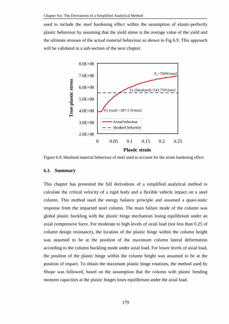
Chapter Six: The Derivations of a Simplified Analytical Method
179
used to include the steel hardening effect within the assumption of elastic-perfectly
plastic behaviour by assuming that the yield stress is the average value of the yield and
the ultimate stresses of the actual material behaviour as shown in Fig 6.9. This approach
will be validated in a sub-section of the next chapter.
Figure 6.9: Idealised material behaviour of steel used to account for the strain hardening effect
6.3. Summary
This chapter has presented the full derivations of a simplified analytical method to
calculate the critical velocity of a rigid body and a flexible vehicle impact on a steel
column. This method used the energy balance principle and assumed a quasi-static
response from the impacted steel column. The main failure mode of the column was
global plastic buckling with the plastic hinge mechanism losing equilibrium under an
axial compressive force. For moderate to high levels of axial load (not less than 0.25 of
column design resistance), the location of the plastic hinge within the column height
was assumed to be at the position of the maximum column lateral deformation
according to the column buckling mode under axial load. For lower levels of axial load,
the position of the plastic hinge within the column height was assumed to be at the
position of impact. To obtain the maximum plastic hinge rotations, the method used by
Shope was followed, based on the assumption that the column with plastic bending
moment capacities at the plastic hinges loses equilibrium under the axial load.
2.0E+08
3.0E+08
4.0E+08
5.0E+08
6.0E+08
7.0E+08
8.0E+08
0 0.05 0.1 0.15 0.2 0.25
Plastic strain
Tru
e pl
astic
str
ess
Actual behaviour
Idealised behaviour
Fy (real) =387.5 N/mm2
Fy (Idealised)=543.75N/mm2
Fu=700N/mm2
Chapter Six: The Derivations of a Simplified Analytical Method
180
A simple approach was suggested in this chapter to calculate the maximum energy
absorbed by the vehicle at column failure. In this approach, the linear behaviour of the
vehicle frontal structure up to the deformation to the engine box is assumed based on
the numerical simulations’ results of chapter five. The maximum vehicle deformation is
determined based on the maximum transverse static resistance of the column. For
design purposes, two alternative approaches were presented in this chapter to calculate
the maximum transverse static resistance of the column, one based on EC3 and the other
proposed by the author.
Chapter seven will present a validation of the proposed method by comparing it against
the numerical simulation results of chapters four and five.

Chapter Seven: Validation of the Simplified Analytical Method
181
Chapter Seven
Validation of the Simplified Analytical Method
7.1. Introduction
The numerical simulation results presented in chapters four and five included the effects
of strain hardening and strain rate. The analytical model proposed in chapter six
assumes an elastic- plastic stress-strain curve without a strain rate effect. A set of new
numerical simulations were carried out using the steel material model assumed in the
analytical approach. The results of these new numerical simulations will be used in this
chapter to ascertain the validity and the accuracy of the proposed analytical method
presented in chapter six. This will be established by comparisons for the column axial
force - critical velocity relationship, the maximum column transverse and axial
displacements - axial force relationship, and for the various energy quantities used in the
simplified energy balance equation. Section 7.2 presents the results for a rigid body
impact and section 7.3 provides additional comparisons for vehicle impact. An
approximation is then proposed in section 7.4 to take into consideration the effect of
strain-hardening. As has been demonstrated in section 4.2.4.7 in chapter four, the effect
of strain rate may be safely ignored for vehicle impact on columns.
In the validation examples, the steel material is assumed to be S355, with a modulus of
elasticity of 206×109 N/m2 and a yield stress of 355×106 N/m2. Table 7.1 lists the
numerical simulations conducted and the column properties used in the validation study.

Chapter Seven: Validation of the Simplified Analytical Method
182
Table 7.1: Properties of the columns used to validate the simplified analytical method
Impact
analysis
Column
length
( m)
Column section
Slenderne
ss ratio
( )z z
kL
r −
Relative
slenderness
yz z
FkL
r Eλ
π− =
Design
axial
compressiv
e load (kN)
Boundary
conditions R
igid
impa
ct
4 UC
305×305×118
51.50
36.05
0.68
0.476
3800
4250
S.S
Prop.
8 UC
356×406×340 76.9 1.02 6800 S.S
Veh
icle
impa
ct 4
UC
254×254×89
61
42.7
0.81
0.564
2580
3200
S.S
Prop.
4 UC
305×305×118
51.50
36.05
0.68
0.476
3800
4250
S.S
Prop.
4 UC
356×368×202 41.66 0.55 6780 S.S
7.2 Validation of the analytical method against rigid body impact
This section aims to validate the analytical method for a range of values for impact
location, impact mass, slenderness ratio and for two boundary conditions. Comparisons
are made between the analytical and the ABAQUS simulation results for the following
quantities: maximum column displacement, critical impact velocity - axial force
relationship, and various energy quantities involved in the analytical method. The
correct calculation of the maximum column displacements is important because it
directly determines the energy absorption of the column and the work undertaken by the
axial force.
7.2.1. Maximum column displacements
The column’s internal energy and the external work done by the column axial load, as
derived in chapter six, depend critically on the value of the maximum column transverse
displacement and the axial displacement (shortening). The maximum energy absorption
capacity of the column corresponds to the maximum column deformation before losing
stability. In the analytical approach, this displacement was derived based on a quasi-
static approximation of column behaviour under a compressive axial load and in global
buckling failure mode. It represents the state of column behaviour which has a zero
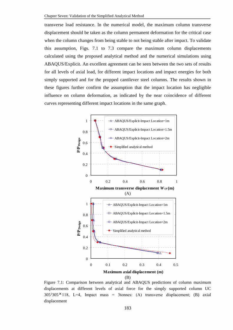
Chapter Seven: Validation of the Simplified Analytical Method
183
transverse load resistance. In the numerical model, the maximum column transverse
displacement should be taken as the column permanent deformation for the critical case
when the column changes from being stable to not being stable after impact. To validate
this assumption, Figs. 7.1 to 7.3 compare the maximum column displacements
calculated using the proposed analytical method and the numerical simulations using
ABAQUS/Explicit. An excellent agreement can be seen between the two sets of results
for all levels of axial load, for different impact locations and impact energies for both
simply supported and for the propped cantilever steel columns. The results shown in
these figures further confirm the assumption that the impact location has negligible
influence on column deformation, as indicated by the near coincidence of different
curves representing different impact locations in the same graph.
0
0.2
0.4
0.6
0.8
1
0 0.2 0.4 0.6 0.8 1
Maximum transverse displacement W cr (m)
P/P
Des
ign
ABAQUS/Explicit-Impact Location=1m
ABAQUS/Explicit-Impact Location=1.5m
ABAQUS/Explicit-Impact Location=2m
Simplified analytical method
(A)
0
0.2
0.4
0.6
0.8
1
0 0.1 0.2 0.3 0.4 0.5
Maximum axial displacement (m)
P/P
Des
ign
ABAQUS/Explicit-Impact Location=1m
ABAQUS/Explicit-Impact Location=1.5m
ABAQUS/Explicit-Impact Location=2m
Simplified analytical method
(B)
Figure 7.1: Comparison between analytical and ABAQUS predictions of column maximum
displacements at different levels of axial force for the simply supported column UC
305×305×118, L=4, Impact mass = 3tonnes: (A) transverse displacement; (B) axial
displacement
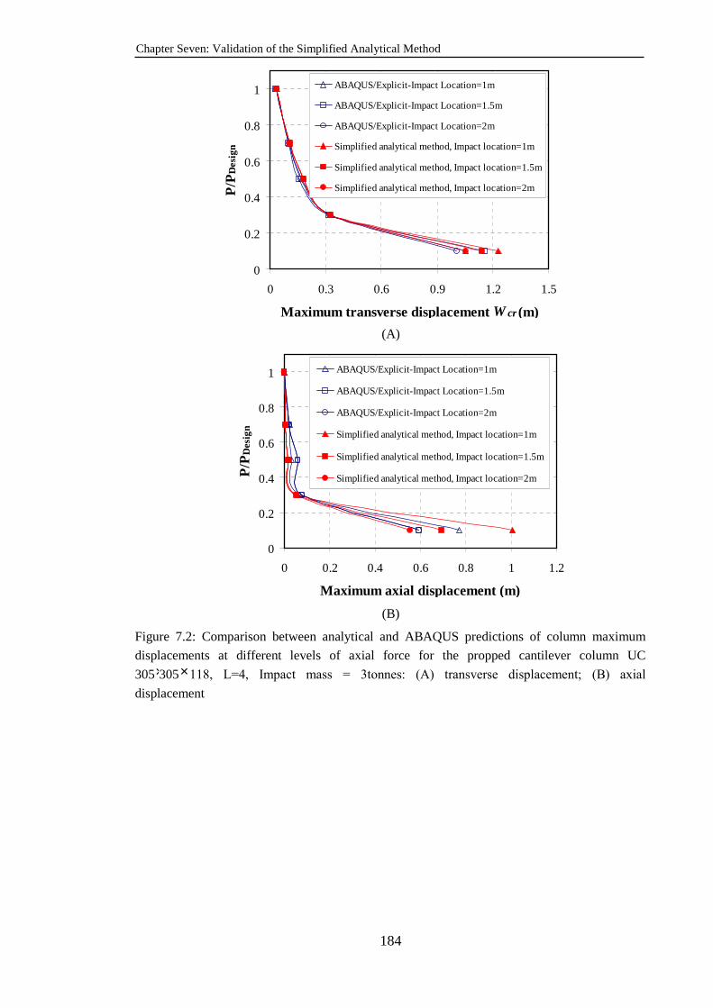
Chapter Seven: Validation of the Simplified Analytical Method
184
0
0.2
0.4
0.6
0.8
1
0 0.3 0.6 0.9 1.2 1.5
Maximum transverse displacement W cr (m)
P/P
De
sig
n
ABAQUS/Explicit-Impact Location=1m
ABAQUS/Explicit-Impact Location=1.5m
ABAQUS/Explicit-Impact Location=2m
Simplified analytical method, Impact location=1m
Simplified analytical method, Impact location=1.5m
Simplified analytical method, Impact location=2m
(A)
0
0.2
0.4
0.6
0.8
1
0 0.2 0.4 0.6 0.8 1 1.2
Maximum axial displacement (m)
P/P
Des
ign
ABAQUS/Explicit-Impact Location=1m
ABAQUS/Explicit-Impact Location=1.5m
ABAQUS/Explicit-Impact Location=2m
Simplified analytical method, Impact location=1m
Simplified analytical method, Impact location=1.5m
Simplified analytical method, Impact location=2m
(B)
Figure 7.2: Comparison between analytical and ABAQUS predictions of column maximum
displacements at different levels of axial force for the propped cantilever column UC
305×305×118, L=4, Impact mass = 3tonnes: (A) transverse displacement; (B) axial
displacement

Chapter Seven: Validation of the Simplified Analytical Method
185
0
0.2
0.4
0.6
0.8
1
0 0.4 0.8 1.2 1.6 2 2.4
Maximum transverse displacement W cr (m)
P/P
Des
ign
ABAQUS/Explicit-Impact Location=1m
ABAQUS/Explicit-Impact Location=2m
ABAQUS/Explicit-Impact Location=2m
Simplified analytical method
(A)
0
0.2
0.4
0.6
0.8
1
0 0.4 0.8 1.2 1.6 2
Maximum transverse displacement W cr (m)
P/P
Des
ign
ABAQUS/Explicit-Impact Location=2m
ABAQUS/Explicit-Impact Location=4m
Simplified analytical method
(B)
Figure 7.3: Comparison between analytical and ABAQUS predictions of column maximum
transverse displacements at different levels of axial force for the simply supported column UC
356×406×340, L=8m, (A) Impact mass = 3tonnes; (B) Impact mass = 6tonnes
7.2.2. Critical impact velocity-axial load interaction curves
Figs. 7.4 to 7.6 compare the critical impact velocity-axial force curves between the
analytical method and the numerical simulation results for different column sections
(UC 356×406×340 and UC 305×305×118), two different boundary conditions (simply
supported and fix-ended) and two impact masses (3 tonnes and 6 tonnes). For the
simply supported columns (Figs. 7.4(A), 7.5 (impact locations=2m and 4m) and 7.6
(impact locations=2m and 4m)), very good correlation is obtained. As the impact
location moves closer to the column base, the difference between the analytical and the
simulation results increases. This reflects the increasing error of assuming the
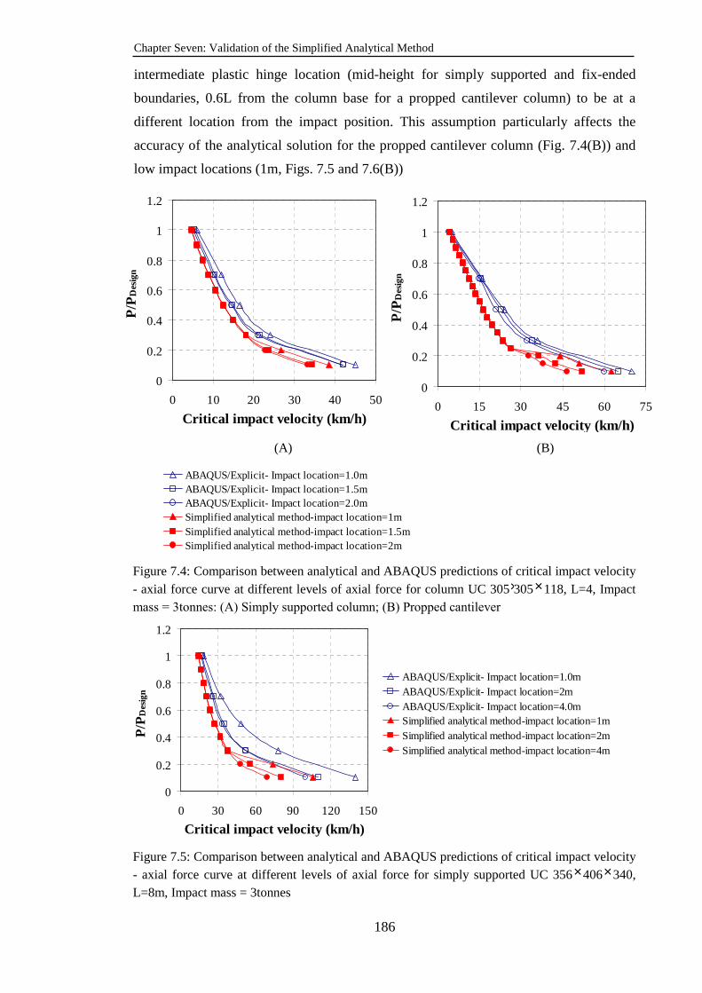
Chapter Seven: Validation of the Simplified Analytical Method
186
intermediate plastic hinge location (mid-height for simply supported and fix-ended
boundaries, 0.6L from the column base for a propped cantilever column) to be at a
different location from the impact position. This assumption particularly affects the
accuracy of the analytical solution for the propped cantilever column (Fig. 7.4(B)) and
low impact locations (1m, Figs. 7.5 and 7.6(B))
(A) (B)
ABAQUS/Explicit- Impact location=1.0mABAQUS/Explicit- Impact location=1.5mABAQUS/Explicit- Impact location=2.0mSimplified analytical method-impact location=1mSimplified analytical method-impact location=1.5mSimplified analytical method-impact location=2m
Figure 7.4: Comparison between analytical and ABAQUS predictions of critical impact velocity - axial force curve at different levels of axial force for column UC 305×305×118, L=4, Impact mass = 3tonnes: (A) Simply supported column; (B) Propped cantilever
0
0.2
0.4
0.6
0.8
1
1.2
0 30 60 90 120 150
Critical impact velocity (km/h)
P/P
Des
ign
ABAQUS/Explicit- Impact location=1.0mABAQUS/Explicit- Impact location=2mABAQUS/Explicit- Impact location=4.0mSimplified analytical method-impact location=1mSimplified analytical method-impact location=2mSimplified analytical method-impact location=4m
Figure 7.5: Comparison between analytical and ABAQUS predictions of critical impact velocity - axial force curve at different levels of axial force for simply supported UC 356×406×340, L=8m, Impact mass = 3tonnes
0
0.2
0.4
0.6
0.8
1
1.2
0 10 20 30 40 50
Critical impact velocity (km/h)
P/P
Des
ign
0
0.2
0.4
0.6
0.8
1
1.2
0 15 30 45 60 75
Critical impact velocity (km/h)
P/P
Des
ign
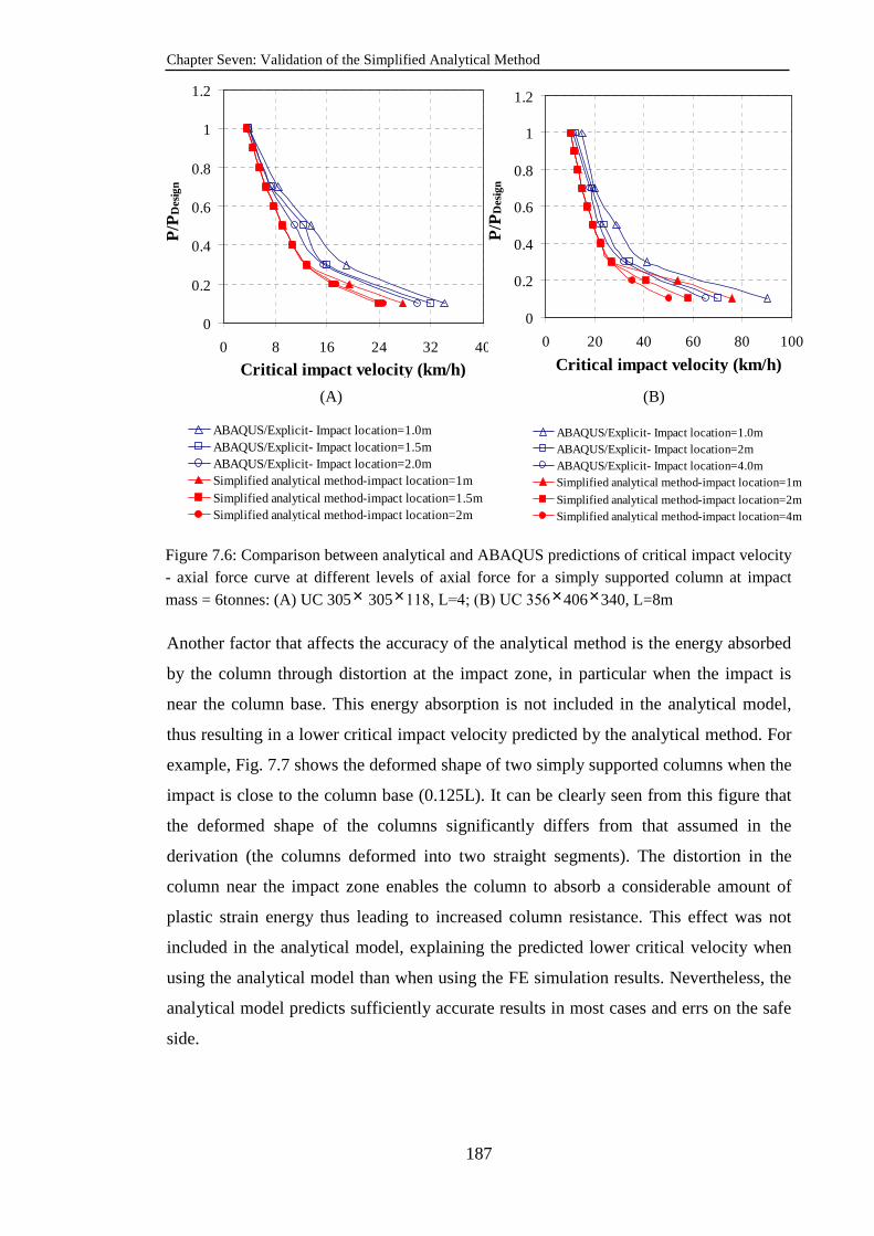
Chapter Seven: Validation of the Simplified Analytical Method
187
(A) (B)
Figure 7.6: Comparison between analytical and ABAQUS predictions of critical impact velocity - axial force curve at different levels of axial force for a simply supported column at impact mass = 6tonnes: (A) UC 305× 305×118, L=4; (B) UC 356×406×340, L=8m
Another factor that affects the accuracy of the analytical method is the energy absorbed
by the column through distortion at the impact zone, in particular when the impact is
near the column base. This energy absorption is not included in the analytical model,
thus resulting in a lower critical impact velocity predicted by the analytical method. For
example, Fig. 7.7 shows the deformed shape of two simply supported columns when the
impact is close to the column base (0.125L). It can be clearly seen from this figure that
the deformed shape of the columns significantly differs from that assumed in the
derivation (the columns deformed into two straight segments). The distortion in the
column near the impact zone enables the column to absorb a considerable amount of
plastic strain energy thus leading to increased column resistance. This effect was not
included in the analytical model, explaining the predicted lower critical velocity when
using the analytical model than when using the FE simulation results. Nevertheless, the
analytical model predicts sufficiently accurate results in most cases and errs on the safe
side.
0
0.2
0.4
0.6
0.8
1
1.2
0 8 16 24 32 40
Critical impact velocity (km/h)
P/P
Des
ign
0
0.2
0.4
0.6
0.8
1
1.2
0 20 40 60 80 100
Critical impact velocity (km/h)
P/P
Des
ign
ABAQUS/Explicit- Impact location=1.0mABAQUS/Explicit- Impact location=1.5mABAQUS/Explicit- Impact location=2.0mSimplified analytical method-impact location=1mSimplified analytical method-impact location=1.5mSimplified analytical method-impact location=2m
ABAQUS/Explicit- Impact location=1.0mABAQUS/Explicit- Impact location=2mABAQUS/Explicit- Impact location=4.0mSimplified analytical method-impact location=1m
Simplified analytical method-impact location=2mSimplified analytical method-impact location=4m
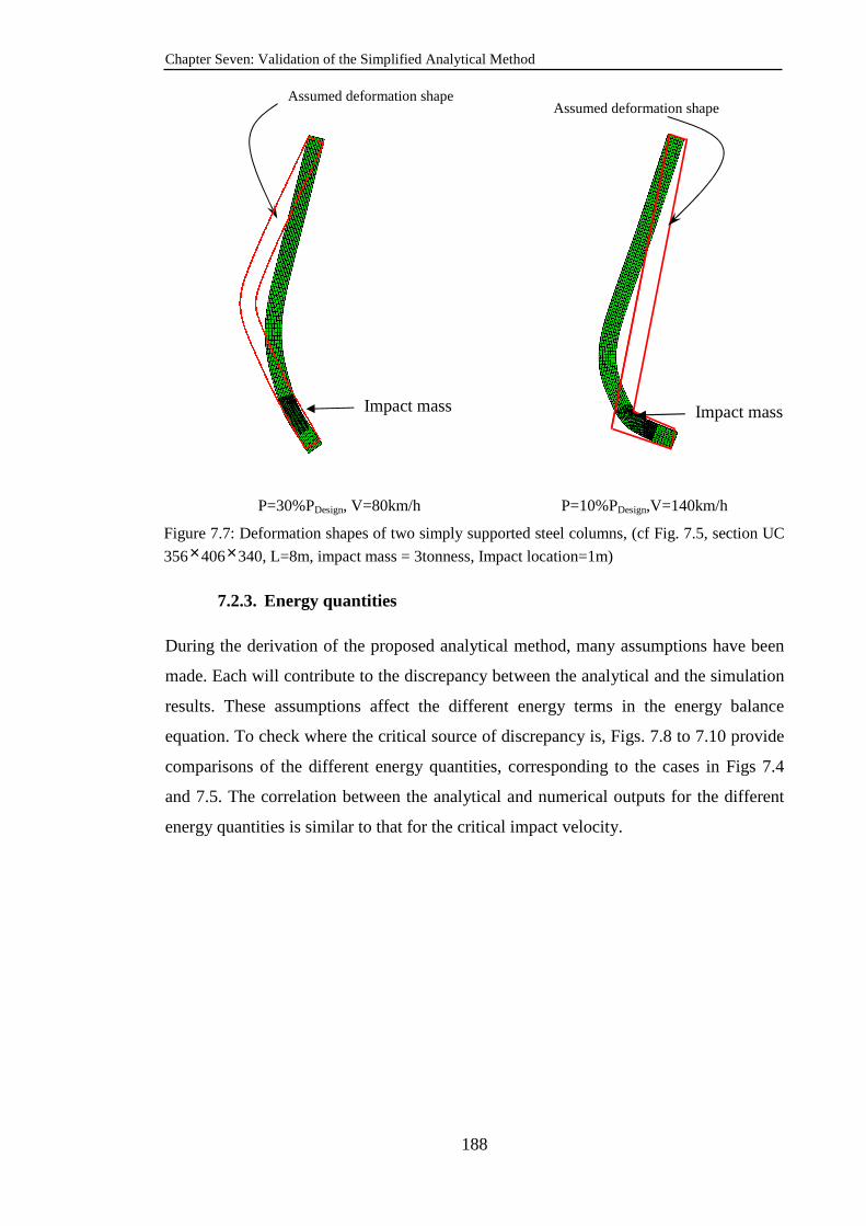
Chapter Seven: Validation of the Simplified Analytical Method
188
P=30%PDesign, V=80km/h P=10%PDesign,V=140km/h
Figure 7.7: Deformation shapes of two simply supported steel columns, (cf Fig. 7.5, section UC
356×406×340, L=8m, impact mass = 3tonness, Impact location=1m)
7.2.3. Energy quantities
During the derivation of the proposed analytical method, many assumptions have been
made. Each will contribute to the discrepancy between the analytical and the simulation
results. These assumptions affect the different energy terms in the energy balance
equation. To check where the critical source of discrepancy is, Figs. 7.8 to 7.10 provide
comparisons of the different energy quantities, corresponding to the cases in Figs 7.4
and 7.5. The correlation between the analytical and numerical outputs for the different
energy quantities is similar to that for the critical impact velocity.
Impact mass
Assumed deformation shape
Impact mass
Assumed deformation shape
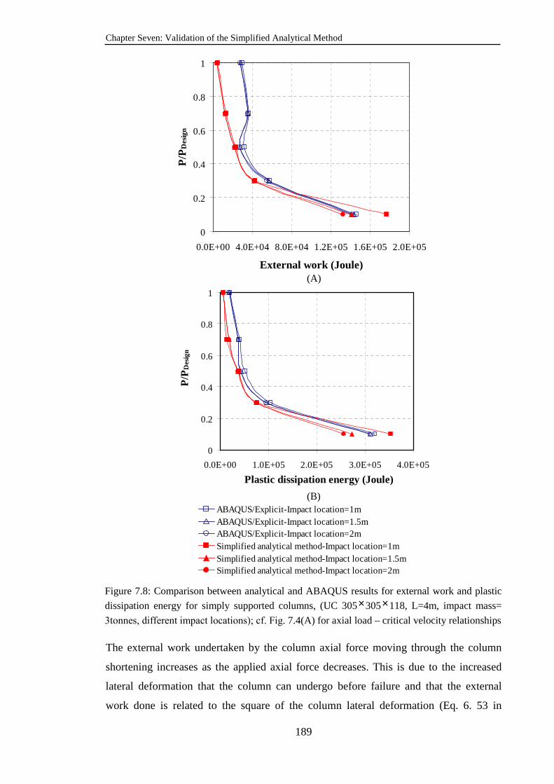
Chapter Seven: Validation of the Simplified Analytical Method
189
0
0.2
0.4
0.6
0.8
1
0.0E+00 4.0E+04 8.0E+04 1.2E+05 1.6E+05 2.0E+05
External work (Joule)
P/P
Des
ign
(A)
0
0.2
0.4
0.6
0.8
1
0.0E+00 1.0E+05 2.0E+05 3.0E+05 4.0E+05
Plastic dissipation energy (Joule)
P/P
Des
ign
(B)
ABAQUS/Explicit-Impact location=1mABAQUS/Explicit-Impact location=1.5mABAQUS/Explicit-Impact location=2mSimplified analytical method-Impact location=1mSimplified analytical method-Impact location=1.5mSimplified analytical method-Impact location=2m
Figure 7.8: Comparison between analytical and ABAQUS results for external work and plastic
dissipation energy for simply supported columns, (UC 305×305×118, L=4m, impact mass=
3tonnes, different impact locations); cf. Fig. 7.4(A) for axial load – critical velocity relationships
The external work undertaken by the column axial force moving through the column
shortening increases as the applied axial force decreases. This is due to the increased
lateral deformation that the column can undergo before failure and that the external
work done is related to the square of the column lateral deformation (Eq. 6. 53 in
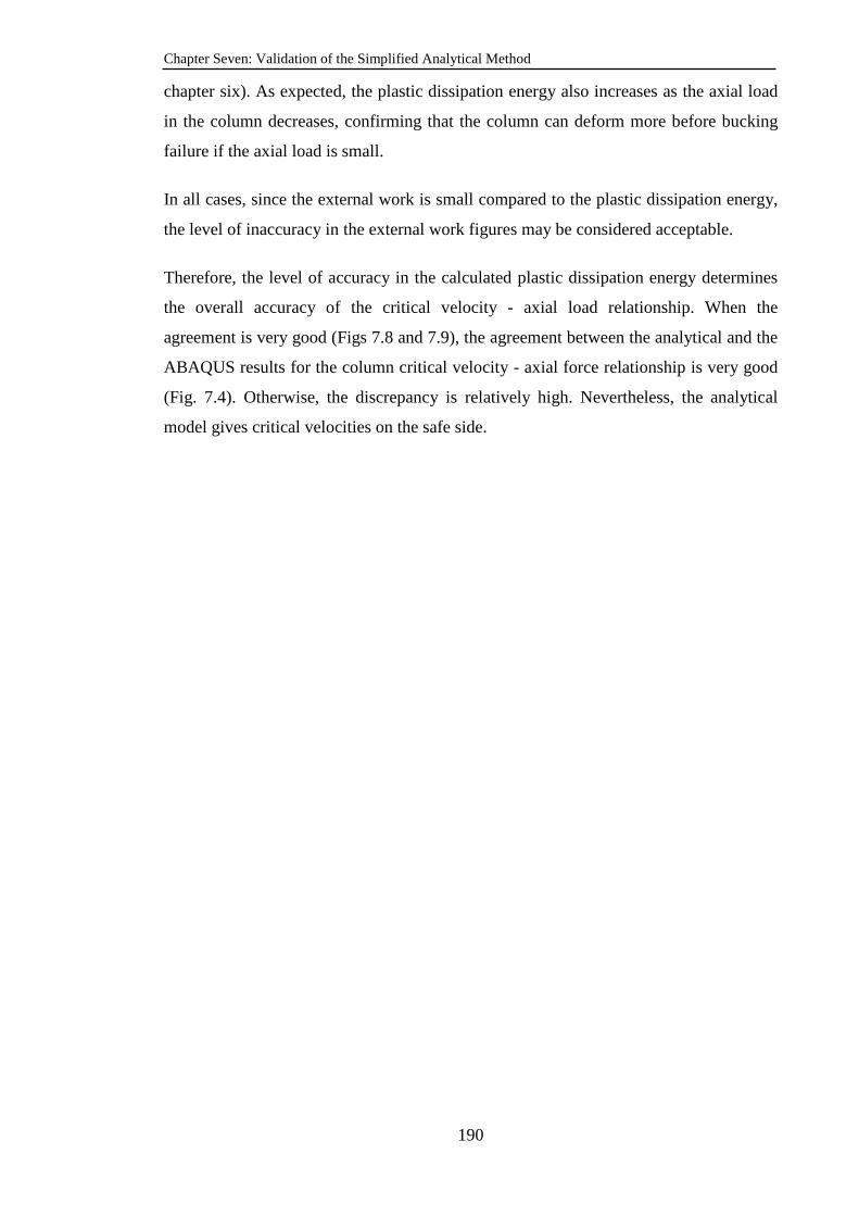
Chapter Seven: Validation of the Simplified Analytical Method
190
chapter six). As expected, the plastic dissipation energy also increases as the axial load
in the column decreases, confirming that the column can deform more before bucking
failure if the axial load is small.
In all cases, since the external work is small compared to the plastic dissipation energy,
the level of inaccuracy in the external work figures may be considered acceptable.
Therefore, the level of accuracy in the calculated plastic dissipation energy determines
the overall accuracy of the critical velocity - axial load relationship. When the
agreement is very good (Figs 7.8 and 7.9), the agreement between the analytical and the
ABAQUS results for the column critical velocity - axial force relationship is very good
(Fig. 7.4). Otherwise, the discrepancy is relatively high. Nevertheless, the analytical
model gives critical velocities on the safe side.
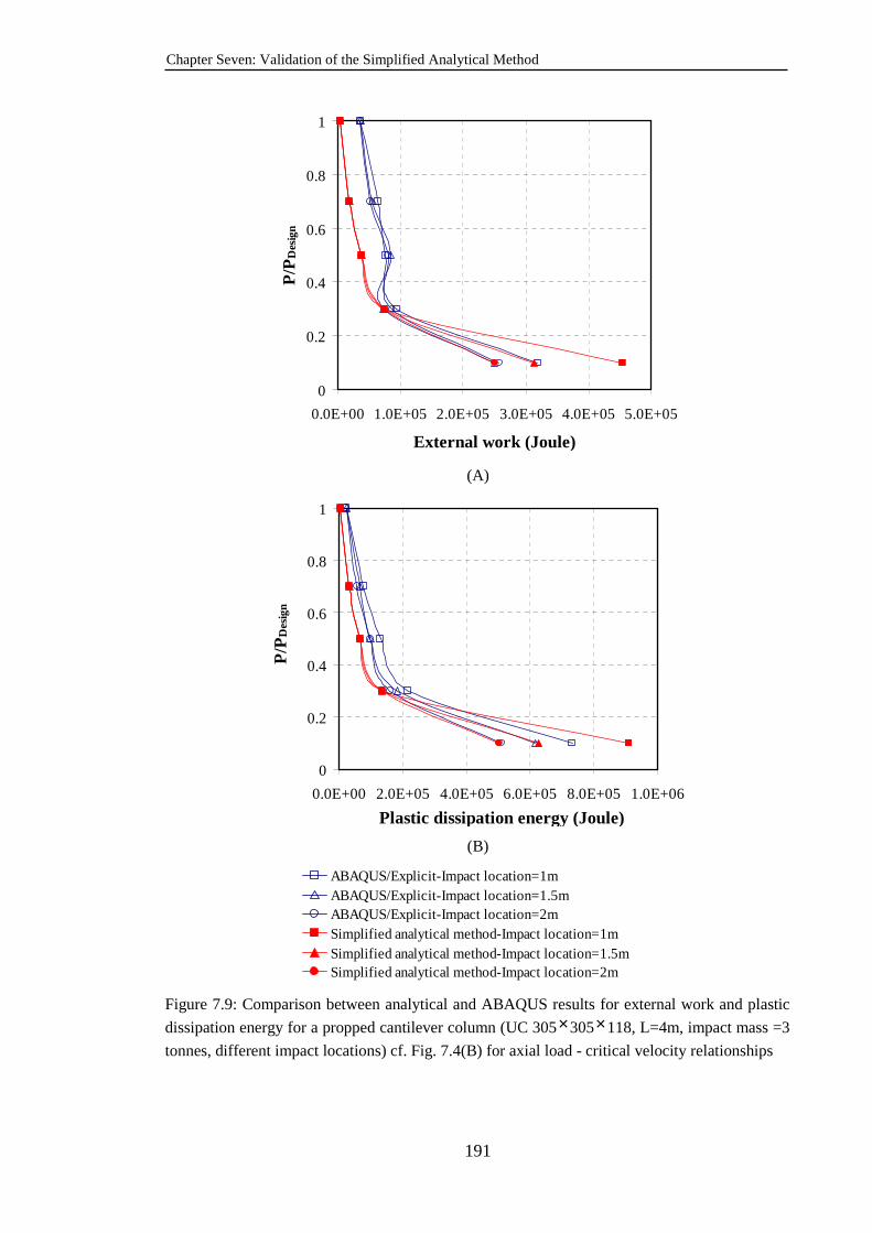
Chapter Seven: Validation of the Simplified Analytical Method
191
0
0.2
0.4
0.6
0.8
1
0.0E+00 1.0E+05 2.0E+05 3.0E+05 4.0E+05 5.0E+05
External work (Joule)
P/P
Des
ign
(A)
0
0.2
0.4
0.6
0.8
1
0.0E+00 2.0E+05 4.0E+05 6.0E+05 8.0E+05 1.0E+06
Plastic dissipation energy (Joule)
P/P
Des
ign
(B)
ABAQUS/Explicit-Impact location=1mABAQUS/Explicit-Impact location=1.5mABAQUS/Explicit-Impact location=2mSimplified analytical method-Impact location=1mSimplified analytical method-Impact location=1.5mSimplified analytical method-Impact location=2m
Figure 7.9: Comparison between analytical and ABAQUS results for external work and plastic
dissipation energy for a propped cantilever column (UC 305×305×118, L=4m, impact mass =3
tonnes, different impact locations) cf. Fig. 7.4(B) for axial load - critical velocity relationships
Chapter Seven: Validation of the Simplified Analytical Method
192
0
0.2
0.4
0.6
0.8
1
0.0E+00 2.4E+05 4.8E+05 7.2E+05 9.6E+05 1.2E+06
External work (Joule)
P/P
Des
ign
(A)
0
0.2
0.4
0.6
0.8
1
0.0E+00 6.0E+05 1.2E+06 1.8E+06 2.4E+06 3.0E+06
Plastic dissipation energy (Joule)
P/P
Des
ign
(B)
ABAQUS/Explicit-Impact location=1mABAQUS/Explicit-Impact location=1.5mABAQUS/Explicit-Impact location=2mSimplified analytical method-Impact location=1mSimplified analytical method-Impact location=1.5mSimplified analytical method-Impact location=2m
Figure 7.10: Comparison between analytical and ABAQUS results for external work and plastic
dissipation energy for a simply supported column (UC 356×406×340, L=8m, impact mass = 3
tonnes, different impact locations), cf. Fig. 7.5 for axial load - critical velocity relationships
In summary, the proposed analytical method provides reasonably accurate predictions
of the critical impact velocities of axially preloaded steel columns under transverse rigid
impact. Comparisons of the different energy quantities indicate good agreement

Chapter Seven: Validation of the Simplified Analytical Method
193
between the numerical and analytical results. This validation suggests that column
behaviour is predicted with good accuracy.
7.3. Validation of the analytical method against vehicle impact
According to the procedure described in chapter six, determination of vehicle
deformation at column global failure requires the input of the column’s resistance to a
static force at the position of impact. This resistance may be obtained using a static
finite element simulation. Fig. 7.11 shows an example of such simulation results. As
explained in section 6.2.3 in chapter six, this resistance may also be determined
analytically, using the method in Eurocode 3 or the newly developed proposal within
this research. In this validation research, the ABAQUS simulation results are first used
to ensure any error from estimating the column transverse resistance is minimized.
Afterwards, in section 7.3.4, the effects of using different methods to predict column
transverse resistance are evaluated.
0.E+00
1.E+05
2.E+05
3.E+05
4.E+05
5.E+05
6.E+05
0 60 120 180 240 300
Transverse displacement (mm)
Late
ral r
esis
tanc
e fo
rce
(N)
(P/P )=1
(P/P )=0.85
(P/P )=0.65
(P/P )=0.43
(P/P )=0.25
(P/P )=0.085
Design
Design
Design
Design
Design
Design
Figure 7.11: Numerical simulations’ results for the transverse force - transverse displacement
relationship of a simply supported column UC 305×305×118 under different axial load ratios.
The maximum vehicle deformation is determined by substituting the column transverse
resistance into Eq. 6.35 in chapter six. Tables 7.2 to 7.4 compare the calculated values
of vehicle maximum deformation with the numerical simulation results. The values of
the vehicle frontal stiffness (K1) are 510kN/m, 463kN/m and 546 kN/m as calculated in
section 5.3.1 in chapter five representing the stiffness of the Chevrolet pick-up 1994
vehicle impacting on steel columns with section sizes of UC 305×305×118, UC
254×254×89 and UC 356×368×202 respectively. Good agreement is achieved between

Chapter Seven: Validation of the Simplified Analytical Method
194
the two sets of results. In the case of vehicle deformation before touching the vehicle
engine, the numerical and analytical values of vehicle deformation are very close. When
the vehicle deformation reaches the engine position, it is assumed that the vehicle acts
as a rigid impactor and does not consume any impact energy. This is indicated in Tables
7.2 to 7.4 by the symbol > Cmax. It is clear that the analytical method has correctly
predicted this in all cases. Table 7.2: The calculated values of vehicle maximum deformation as compared with the
numerical simulation results for a steel column section UC 305×305×118, K1=510kN/m
Simply supported column Propped cantilever column
P/PDesign Crush displacement, C(m)
P/PDesign Crush displacement, C(m)
Analytical ABAQUS Analytical ABAQUS
1 0.233 0.247 1 0.454 0.461
0.85 0.401 0.424 0.82 > Cmax
(0.625) > Cmax
0.65 > Cmax > Cmax 0.60 > Cmax > Cmax 0.43 > Cmax > Cmax 0.40 > Cmax > Cmax
0.25 > Cmax > Cmax 0.25 > Cmax > Cmax
Table 7.3: The calculated values of vehicle maximum deformation as compared with the
numerical simulation results for a steel column section UC 254×254×89, K1=463kN/m
Simply supported column Propped cantilever column
P/PDesign Crush displacement, C (m)
P/PDesign Crush displacement, C (m)
Analytical ABAQUS Analytical ABAQUS
1 0.169 0.181 1 0.357 0.373
0.85 0.261 0.273 0.85 0.6 >Cmax
(0.625) 0.65 0.44 0.456 0.65 >Cmax >Cmax 0.43 0.6 0.613 0.43 >Cmax >Cmax
0.25 >Cmax >Cmax 0.25 >Cmax >Cmax
Table 7.4: The calculated values of vehicle maximum deformation as compared with the
numerical simulation results for a steel column section UC 356×368×202, K1=546kN/m
Simply supported column
P/PDesign
Crush displacement, C(m)
Analytical ABAQUS
1 0.622 0.51 0.85 >Cmax >Cmax 0.65 >Cmax >Cmax 0.43 >Cmax >Cmax
0.25 >Cmax >Cmax

Chapter Seven: Validation of the Simplified Analytical Method
195
7.3.1. Critical impact velocity- axial load interaction curves
Having determined the vehicle deformation, the energy balance equations derived in
chapter six can be used now to determine the critical impact velocity of the vehicle that
can cause the failure of steel columns. Figs. 7.12 to 7.14 compare the numerical and
analytical results. Good agreement can be seen between the two sets of results,
especially for simply supported columns and for columns with high axial load ratios.
Including the effects of vehicle stiffness gives much higher critical impact velocities
than assuming a rigid impact mass. This considerable difference in column critical
impact velocity highlights the importance of including the energy absorbed by the
vehicle in design.
(A) (B)
Figure 7.12: Comparison between analytical and ABAQUS predictions of critical impact
velocity - axial force curve at different levels of axial force for the steel column section UC
254×254×89: (A) simply supported column (B) propped cantilever column.
0
0.2
0.4
0.6
0.8
1
1.2
0 9 18 27 36 45Critical impact velocity (km/h)
(P/P
Des
ign)
Rigid/ ABAQUSRigid/ AnalyticalVehicle / ABAQUSVehicle/ Analytical
0
0.2
0.4
0.6
0.8
1
1.2
0 12 24 36 48 60
Critical impact velocity (km/h)
(P/P
Des
ign)
Rigid/ ABAQUSRigid/ AnalyticalVehicle/ ABAQUSVehicle/ Analytical

Chapter Seven: Validation of the Simplified Analytical Method
196
(A) (B)
Figure 7.13: Comparison between analytical and ABAQUS predictions of critical impact
velocity - axial force curve at different levels of axial force for the steel column section UC
305×305×118: (A) simply supported column; (B) propped cantilever column.
0
0.2
0.4
0.6
0.8
1
1.2
0 20 40 60 80Critical impact velocity (km/h)
( P/P
De
sig
n)
Rigid/ ABAQUS
Rigid/ Analytical
Vehicle/ ABAQUS
Vehicle/ Analytical
Figure 7.14: Comparison between analytical and ABAQUS predictions of critical impact
velocity - axial force curve at different levels of axial force for the simply supported steel
column section UC 356×368×202.
The change in accuracy at different column axial load levels (that is, being better at
higher axial loads) may be explained by the role played by the vehicle. Figs. 7.15 and
7.16 compare the analytical and the simulation values of energy absorption by the
vehicle. The agreement is excellent, confirming the accuracy of the vehicle model. At
high column axial loads, as shown in Tables 7.2 to 7.4, column failure was before the
vehicle had deformed to the engine position. The accuracy of the analytical method
0
0.2
0.4
0.6
0.8
1
1.2
0 20 40 60 80
Critical impact velocity (km/h)
(P/P
Des
ign)
Rigid/ ABAQUS
Rigid/ Analytical
Vehicle/ ABAQUS
Vehicle/ Analytical
0
0.2
0.4
0.6
0.8
1
1.2
0 15 30 45 60
Critical impact velocity (km/h)
(P/P
Des
ign)
Rigid/ ABAQUSRigid/ AnalyticalVehicle/ ABAQUSVehicle/ Analytical

Chapter Seven: Validation of the Simplified Analytical Method
197
depends largely on the accuracy of predicting vehicle behaviour, hence the good
accuracy achieved for the vehicle energy absorption is reflected in the good accuracy of
the overall prediction of the critical impact velocity. When column failure occurs after
contacting the vehicle engine (Fig.7.13(B) and Fig.7.14), the value of the energy
absorbed by the vehicle was constant and equal to the maximum energy absorption
capacity of the vehicle (Eq. 6.36 in chapter six). Therefore, in this case, the accuracy of
predicting the critical impact velocity depends solely upon the accuracy of predicting
the energy absorbed by the column. As shown in section 7.2 which discussed the rigid
body impact, there was high inaccuracy under some conditions.
Figure 7.15: Comparison between analytical and ABAQUS results for energy absorbed by vehicle for the steel column section UC 305×305×118: (A) simply supported column; (B)
propped cantilever column.
Figure 7.16: Comparison between analytical and ABAQUS results for energy absorbed by
vehicle for the steel column section UC 254×254×89: (A) simply supported column; (B)
propped cantilever column.
0
0.2
0.4
0.6
0.8
1
1.2
0.E+00 2.E+04 4.E+04 6.E+04 8.E+04 1.E+05
Energy absorbed by vehicle (Joule)
(P/P
De
sig
n)
ABAQUS
Analytical0
0.2
0.4
0.6
0.8
1
1.2
0.0E+00 2.4E+04 4.8E+04 7.2E+04 9.6E+04 1.2E+05
Energy absorbed by vehicle (Joule)
(P/P
De
sig
n)
ABAQUS
Analytical
0
0.2
0.4
0.6
0.8
1
1.2
0.0E+00 2.4E+04 4.8E+04 7.2E+04 9.6E+04 1.2E+05
Energy absorbed by vehicle(Joule)
(P/P
De
sig
n)
ABAQUS
Analytical
0
0.2
0.4
0.6
0.8
1
1.2
0.0E+00 2.4E+04 4.8E+04 7.2E+04 9.6E+04 1.2E+05
Energy absorbed by vehicle(Joule))
(P/P
De
sig
n)
ABAQUS
Analytical
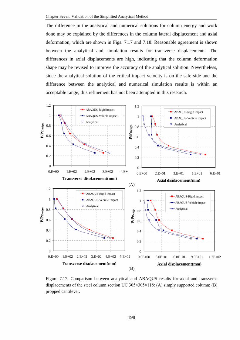
Chapter Seven: Validation of the Simplified Analytical Method
198
The difference in the analytical and numerical solutions for column energy and work
done may be explained by the differences in the column lateral displacement and axial
deformation, which are shown in Figs. 7.17 and 7.18. Reasonable agreement is shown
between the analytical and simulation results for transverse displacements. The
differences in axial displacements are high, indicating that the column deformation
shape may be revised to improve the accuracy of the analytical solution. Nevertheless,
since the analytical solution of the critical impact velocity is on the safe side and the
difference between the analytical and numerical simulation results is within an
acceptable range, this refinement has not been attempted in this research.
(A)
(B)
Figure 7.17: Comparison between analytical and ABAQUS results for axial and transverse
displacements of the steel column section UC 305×305×118: (A) simply supported column; (B)
propped cantilever.
0
0.2
0.4
0.6
0.8
1
1.2
0.E+00 1.E+02 2.E+02 3.E+02 4.E+02
Transverse displacement(mm)
P/P
Des
ign
ABAQUS-Rigid impact
ABAQUS-Vehicle impact
Analytical
0
0.2
0.4
0.6
0.8
1
1.2
0.E+00 2.E+01 3.E+01 5.E+01 6.E+01
Axial displacement(mm)
P/P
Des
ign
ABAQUS-Rigid impact
ABAQUS-Vehicle impact
Analytical
0
0.2
0.4
0.6
0.8
1
1.2
0.0E+00 3.0E+01 6.0E+01 9.0E+01 1.2E+02
Axial displacement(mm)
P/P
Des
ign
ABAQUS-Rigid impact
ABAQUS-Vehicle impact
Analytical
0
0.2
0.4
0.6
0.8
1
1.2
0.E+00 1.E+02 2.E+02 3.E+02 4.E+02 5.E+02
Transverse displacement(mm)
P/P
Des
ign
ABAQUS-Rigid impact
ABAQUS-Vehicle impact
Analytical
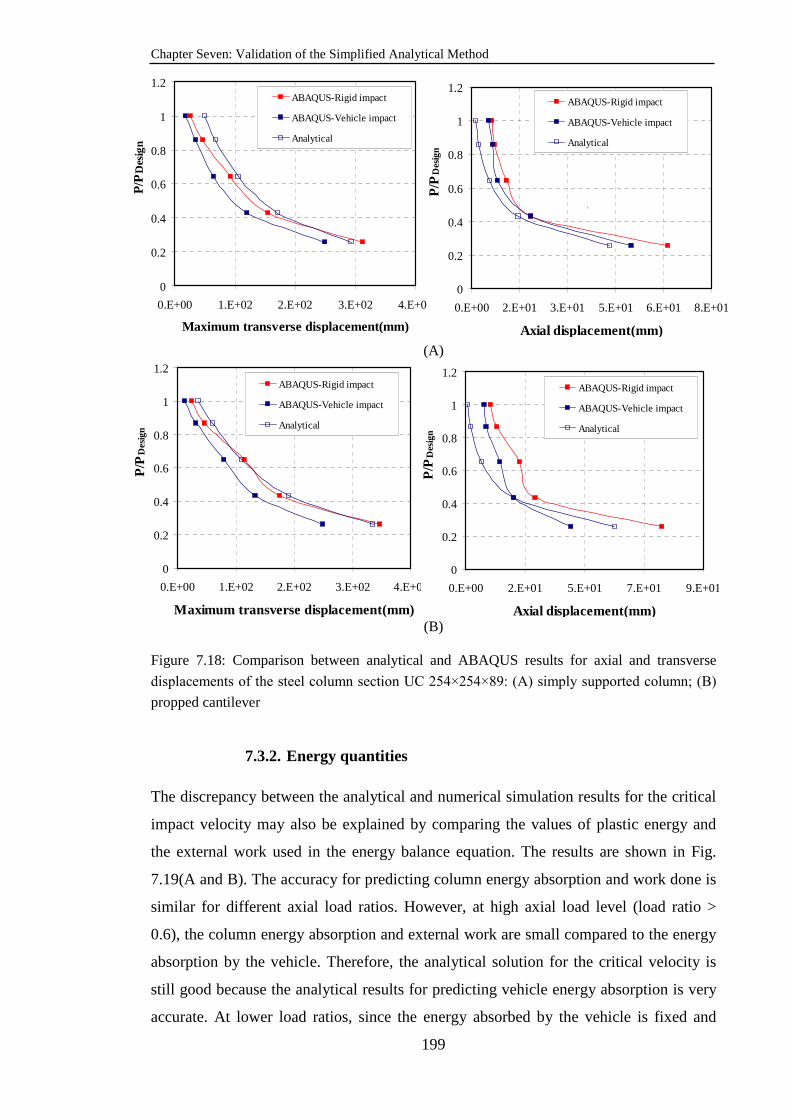
Chapter Seven: Validation of the Simplified Analytical Method
199
(A)
(B)
Figure 7.18: Comparison between analytical and ABAQUS results for axial and transverse
displacements of the steel column section UC 254×254×89: (A) simply supported column; (B)
propped cantilever
7.3.2. Energy quantities
The discrepancy between the analytical and numerical simulation results for the critical
impact velocity may also be explained by comparing the values of plastic energy and
the external work used in the energy balance equation. The results are shown in Fig.
7.19(A and B). The accuracy for predicting column energy absorption and work done is
similar for different axial load ratios. However, at high axial load level (load ratio >
0.6), the column energy absorption and external work are small compared to the energy
absorption by the vehicle. Therefore, the analytical solution for the critical velocity is
still good because the analytical results for predicting vehicle energy absorption is very
accurate. At lower load ratios, since the energy absorbed by the vehicle is fixed and
0
0.2
0.4
0.6
0.8
1
1.2
0.E+00 1.E+02 2.E+02 3.E+02 4.E+02
Maximum transverse displacement(mm)
P/P
Des
ign
ABAQUS-Rigid impact
ABAQUS-Vehicle impact
Analytical
0
0.2
0.4
0.6
0.8
1
1.2
0.E+00 2.E+01 3.E+01 5.E+01 6.E+018.E+01
Axial displacement(mm)
P/P
Des
ign
ABAQUS-Rigid impact
ABAQUS-Vehicle impact
Analytical
`
0
0.2
0.4
0.6
0.8
1
1.2
0.E+00 1.E+02 2.E+02 3.E+02 4.E+02
Maximum transverse displacement(mm)
P/P
Des
ign
ABAQUS-Rigid impact
ABAQUS-Vehicle impact
Analytical
0
0.2
0.4
0.6
0.8
1
1.2
0.E+00 2.E+01 5.E+01 7.E+01 9.E+01
Axial displacement(mm)
P/P
Des
ign
ABAQUS-Rigid impact
ABAQUS-Vehicle impact
Analytical
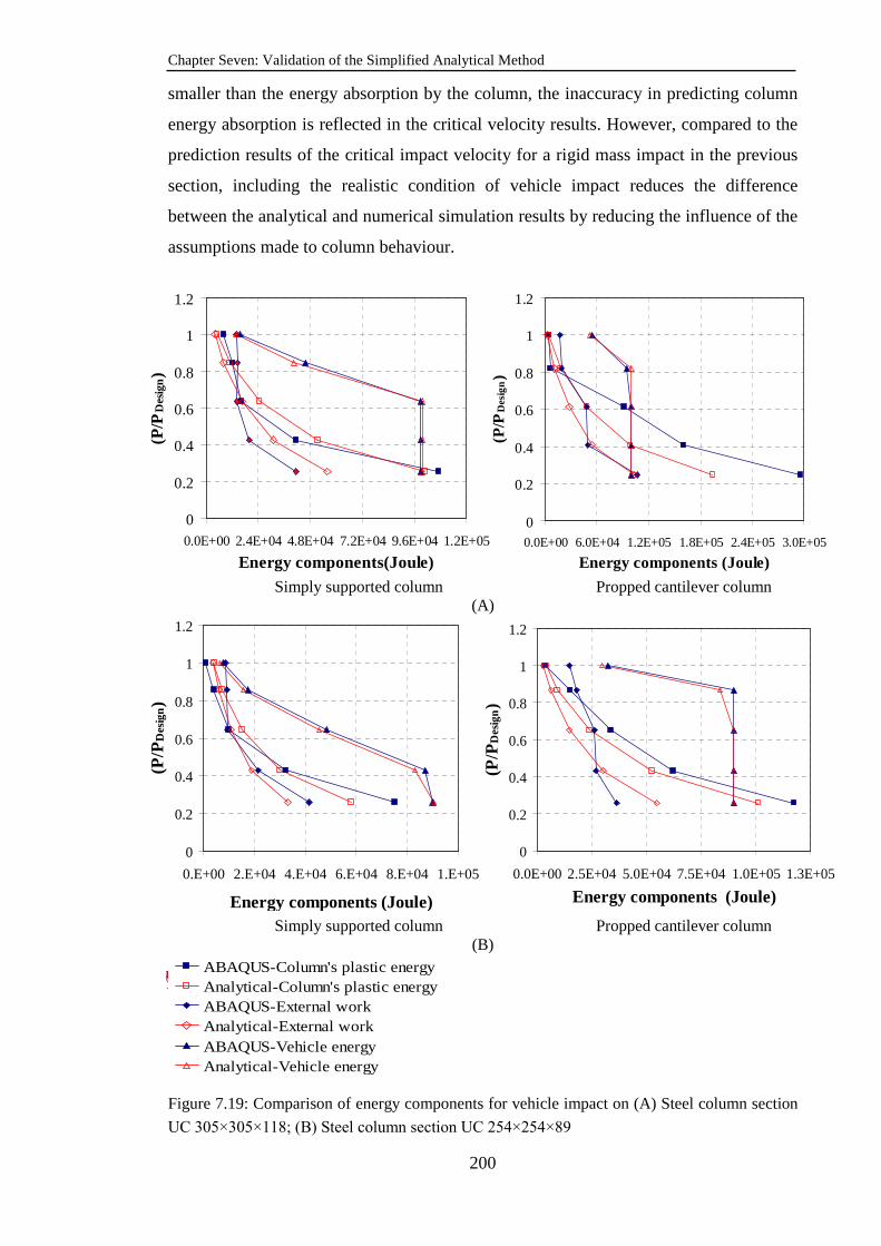
Chapter Seven: Validation of the Simplified Analytical Method
200
smaller than the energy absorption by the column, the inaccuracy in predicting column
energy absorption is reflected in the critical velocity results. However, compared to the
prediction results of the critical impact velocity for a rigid mass impact in the previous
section, including the realistic condition of vehicle impact reduces the difference
between the analytical and numerical simulation results by reducing the influence of the
assumptions made to column behaviour.
Simply supported column Propped cantilever column
(A)
Simply supported column Propped cantilever column
(B) ABAQUS-Column's plastic energyAnalytical-Column's plastic energyABAQUS-External workAnalytical-External workABAQUS-Vehicle energy Analytical-Vehicle energy
Figure 7.19: Comparison of energy components for vehicle impact on (A) Steel column section
UC 305×305×118; (B) Steel column section UC 254×254×89
0
0.2
0.4
0.6
0.8
1
1.2
0.E+00 2.E+04 4.E+04 6.E+04 8.E+04 1.E+05
Energy components (Joule)
(P/P
Des
ign)
0
0.2
0.4
0.6
0.8
1
1.2
0.0E+00 2.5E+04 5.0E+04 7.5E+04 1.0E+05 1.3E+05
Energy components (Joule)
(P/P
Des
ign)
0
0.2
0.4
0.6
0.8
1
1.2
0.0E+00 6.0E+04 1.2E+05 1.8E+05 2.4E+05 3.0E+05
Energy components (Joule)
(P/P
Des
ign)
0
0.2
0.4
0.6
0.8
1
1.2
0.0E+00 2.4E+04 4.8E+04 7.2E+04 9.6E+04 1.2E+05
Energy components(Joule)
(P/P
Des
ign)
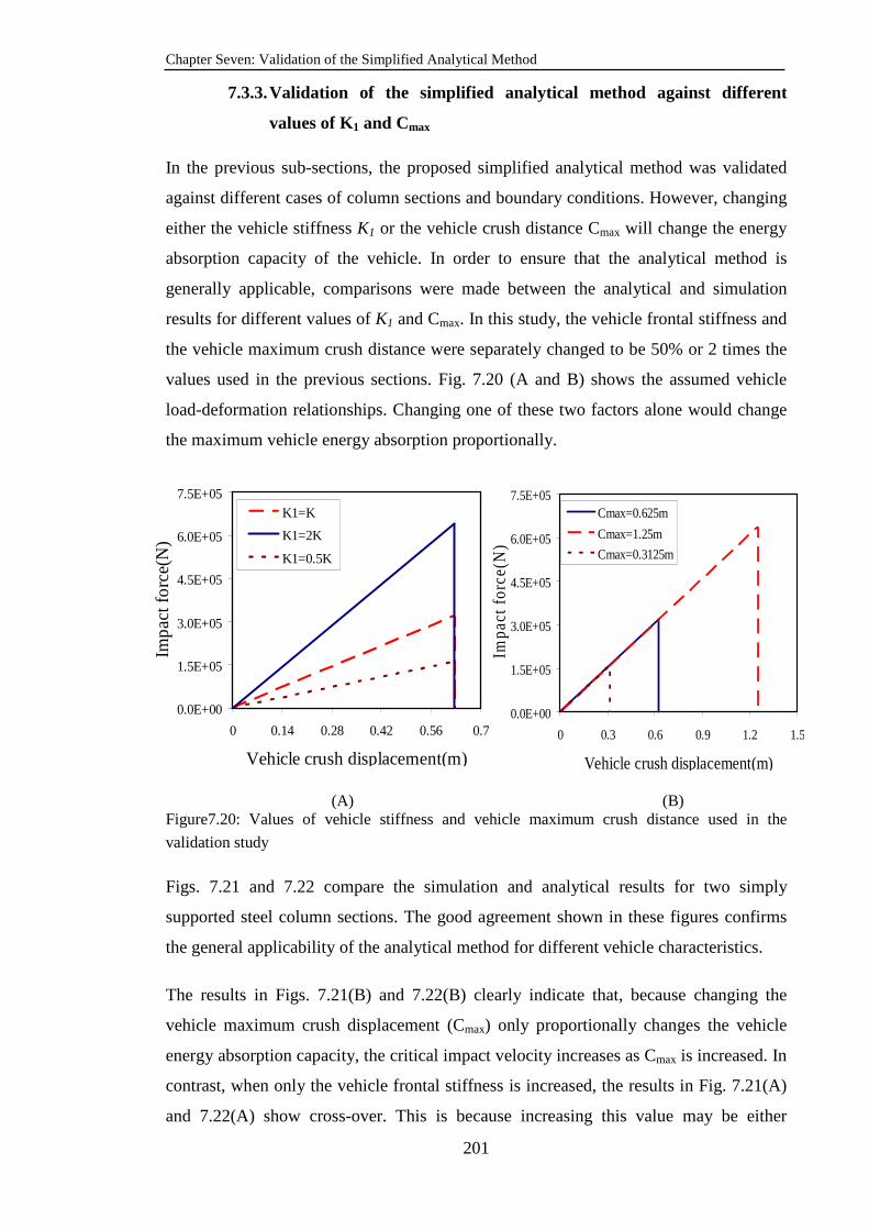
Chapter Seven: Validation of the Simplified Analytical Method
201
7.3.3. Validation of the simplified analytical method against different
values of K1 and Cmax
In the previous sub-sections, the proposed simplified analytical method was validated
against different cases of column sections and boundary conditions. However, changing
either the vehicle stiffness K1 or the vehicle crush distance Cmax will change the energy
absorption capacity of the vehicle. In order to ensure that the analytical method is
generally applicable, comparisons were made between the analytical and simulation
results for different values of K1 and Cmax. In this study, the vehicle frontal stiffness and
the vehicle maximum crush distance were separately changed to be 50% or 2 times the
values used in the previous sections. Fig. 7.20 (A and B) shows the assumed vehicle
load-deformation relationships. Changing one of these two factors alone would change
the maximum vehicle energy absorption proportionally.
(A) (B) Figure7.20: Values of vehicle stiffness and vehicle maximum crush distance used in the
validation study
Figs. 7.21 and 7.22 compare the simulation and analytical results for two simply
supported steel column sections. The good agreement shown in these figures confirms
the general applicability of the analytical method for different vehicle characteristics.
The results in Figs. 7.21(B) and 7.22(B) clearly indicate that, because changing the
vehicle maximum crush displacement (Cmax) only proportionally changes the vehicle
energy absorption capacity, the critical impact velocity increases as Cmax is increased. In
contrast, when only the vehicle frontal stiffness is increased, the results in Fig. 7.21(A)
and 7.22(A) show cross-over. This is because increasing this value may be either
0.0E+00
1.5E+05
3.0E+05
4.5E+05
6.0E+05
7.5E+05
0 0.14 0.28 0.42 0.56 0.7
Vehicle crush displacement(m)
Imp
act f
orc
e(N
)
K1=K
K1=2K
K1=0.5K
0.0E+00
1.5E+05
3.0E+05
4.5E+05
6.0E+05
7.5E+05
0 0.3 0.6 0.9 1.2 1.5
Vehicle crush displacement(m)
Impa
ct f
orce
(N)
Cmax=0.625m
Cmax=1.25m
Cmax=0.3125m
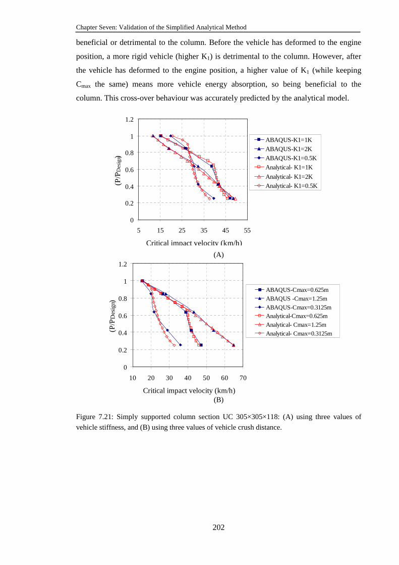
Chapter Seven: Validation of the Simplified Analytical Method
202
beneficial or detrimental to the column. Before the vehicle has deformed to the engine
position, a more rigid vehicle (higher K1) is detrimental to the column. However, after
the vehicle has deformed to the engine position, a higher value of K1 (while keeping
Cmax the same) means more vehicle energy absorption, so being beneficial to the
column. This cross-over behaviour was accurately predicted by the analytical model.
0
0.2
0.4
0.6
0.8
1
1.2
5 15 25 35 45 55
Critical impact velocity (km/h)
(P/P
Des
ign)
ABAQUS-K1=1K
ABAQUS-K1=2K
ABAQUS-K1=0.5K
Analytical- K1=1K
Analytical- K1=2K
Analytical- K1=0.5K
(A)
0
0.2
0.4
0.6
0.8
1
1.2
10 20 30 40 50 60 70
Critical impact velocity (km/h)
(P/P
Des
ign)
ABAQUS-Cmax=0.625m
ABAQUS -Cmax=1.25m
ABAQUS-Cmax=0.3125mAnalytical-Cmax=0.625m
Analytical- Cmax=1.25m
Analytical- Cmax=0.3125m
(B)
Figure 7.21: Simply supported column section UC 305×305×118: (A) using three values of
vehicle stiffness, and (B) using three values of vehicle crush distance.
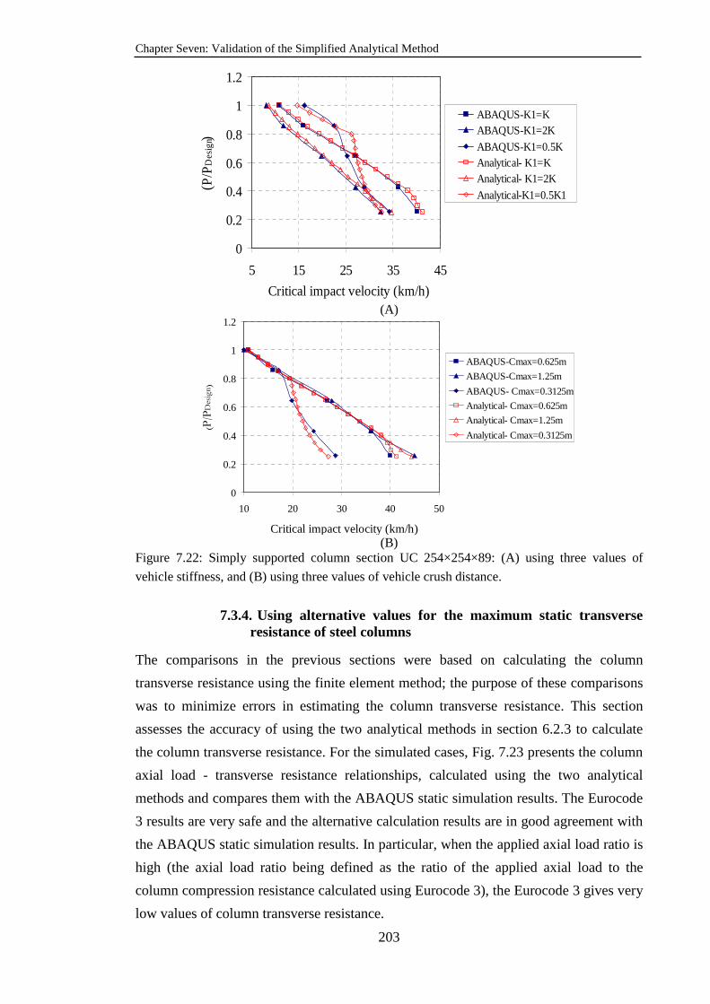
Chapter Seven: Validation of the Simplified Analytical Method
203
0
0.2
0.4
0.6
0.8
1
1.2
5 15 25 35 45
Critical impact velocity (km/h)
(P/P
Des
ign)
ABAQUS-K1=KABAQUS-K1=2K
ABAQUS-K1=0.5KAnalytical- K1=KAnalytical- K1=2K
Analytical-K1=0.5K1
(A)
0
0.2
0.4
0.6
0.8
1
1.2
10 20 30 40 50
Critical impact velocity (km/h)
(P/P
Design)
ABAQUS-Cmax=0.625m
ABAQUS-Cmax=1.25m
ABAQUS- Cmax=0.3125m
Analytical- Cmax=0.625m
Analytical- Cmax=1.25m
Analytical- Cmax=0.3125m
(B)
Figure 7.22: Simply supported column section UC 254×254×89: (A) using three values of
vehicle stiffness, and (B) using three values of vehicle crush distance.
7.3.4. Using alternative values for the maximum static transverse resistance of steel columns
The comparisons in the previous sections were based on calculating the column
transverse resistance using the finite element method; the purpose of these comparisons
was to minimize errors in estimating the column transverse resistance. This section
assesses the accuracy of using the two analytical methods in section 6.2.3 to calculate
the column transverse resistance. For the simulated cases, Fig. 7.23 presents the column
axial load - transverse resistance relationships, calculated using the two analytical
methods and compares them with the ABAQUS static simulation results. The Eurocode
3 results are very safe and the alternative calculation results are in good agreement with
the ABAQUS static simulation results. In particular, when the applied axial load ratio is
high (the axial load ratio being defined as the ratio of the applied axial load to the
column compression resistance calculated using Eurocode 3), the Eurocode 3 gives very
low values of column transverse resistance.
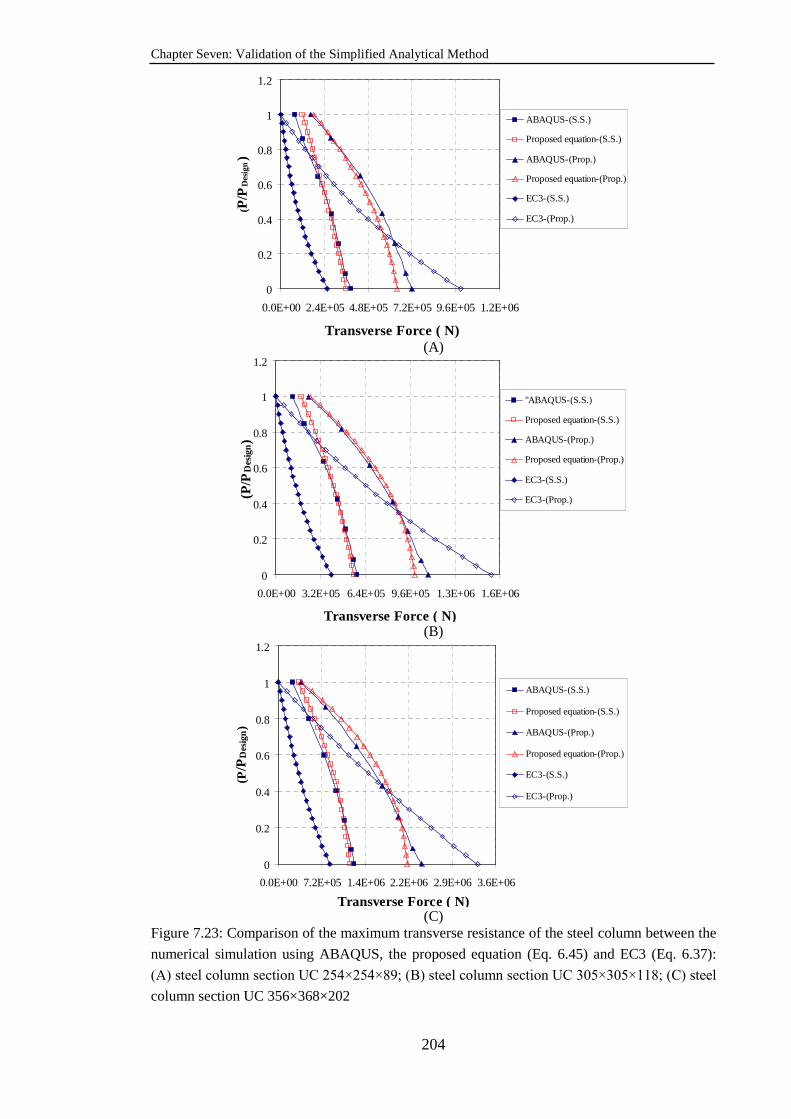
Chapter Seven: Validation of the Simplified Analytical Method
204
0
0.2
0.4
0.6
0.8
1
1.2
0.0E+00 2.4E+05 4.8E+05 7.2E+05 9.6E+05 1.2E+06
Transverse Force ( N)
(P/P
Des
ign)
ABAQUS-(S.S.)
Proposed equation-(S.S.)
ABAQUS-(Prop.)
Proposed equation-(Prop.)
EC3-(S.S.)
EC3-(Prop.)
(A)
0
0.2
0.4
0.6
0.8
1
1.2
0.0E+00 3.2E+05 6.4E+05 9.6E+05 1.3E+06 1.6E+06
Transverse Force ( N)
(P/P
Des
ign)
"ABAQUS-(S.S.)
Proposed equation-(S.S.)
ABAQUS-(Prop.)
Proposed equation-(Prop.)
EC3-(S.S.)
EC3-(Prop.)
(B)
0
0.2
0.4
0.6
0.8
1
1.2
0.0E+00 7.2E+05 1.4E+06 2.2E+06 2.9E+06 3.6E+06
Transverse Force ( N)
(P/P
Des
ign)
ABAQUS-(S.S.)
Proposed equation-(S.S.)
ABAQUS-(Prop.)
Proposed equation-(Prop.)
EC3-(S.S.)
EC3-(Prop.)
(C)
Figure 7.23: Comparison of the maximum transverse resistance of the steel column between the
numerical simulation using ABAQUS, the proposed equation (Eq. 6.45) and EC3 (Eq. 6.37):
(A) steel column section UC 254×254×89; (B) steel column section UC 305×305×118; (C) steel
column section UC 356×368×202
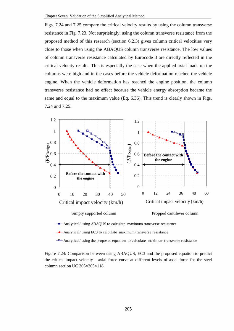
Chapter Seven: Validation of the Simplified Analytical Method
205
Figs. 7.24 and 7.25 compare the critical velocity results by using the column transverse
resistance in Fig. 7.23. Not surprisingly, using the column transverse resistance from the
proposed method of this research (section 6.2.3) gives column critical velocities very
close to those when using the ABAQUS column transverse resistance. The low values
of column transverse resistance calculated by Eurocode 3 are directly reflected in the
critical velocity results. This is especially the case when the applied axial loads on the
columns were high and in the cases before the vehicle deformation reached the vehicle
engine. When the vehicle deformation has reached the engine position, the column
transverse resistance had no effect because the vehicle energy absorption became the
same and equal to the maximum value (Eq. 6.36). This trend is clearly shown in Figs.
7.24 and 7.25.
Simply supported column Propped cantilever column
0
0.5
1
1.5
253545556575
Critical impact velocity (km/h)
(P/P
De
sig
n )
Analytical/ using ABAQUS to calculate maximum transverse resistance
Analytical/ using EC3 to calculate maximum transverse resistance
Analytical/ using the proposed equation to calculate maximum transverse resistance
Figure 7.24: Comparison between using ABAQUS, EC3 and the proposed equation to predict
the critical impact velocity - axial force curve at different levels of axial force for the steel
column section UC 305×305×118.
0
0.2
0.4
0.6
0.8
1
1.2
0 10 20 30 40 50
Critical impact velocity (km/h)
(P/P
Des
ign)
0
0.2
0.4
0.6
0.8
1
1.2
0 12 24 36 48 60
Critical impact velocity (km/h)
(P/P
Des
ign)
Before the contact with the engine
Before the contact with the engine

Chapter Seven: Validation of the Simplified Analytical Method
206
Simply supported column Propped cantilever column
0
0.5
1
1.5
253545556575
Critical impact velocity (km/h)
(P/P
De
sig
n )
Analytical/ using ABAQUS to calculate maximum transverse resistance
Analytical/ using EC3 to calculate maximum transverse resistance
Analytical/ using the proposed equation to calculate maximum transverse resistance
Figure 7.25: Comparison between using ABAQUS, EC3 and the proposed equation to predict
the critical impact velocity - axial force curve at different levels of axial force for the steel
column section UC 254×254×89.
7.4. The strain hardening effect
Section 6.2.6 in chapter six has explained how the strain hardening effect of steel may
be incorporated in the analytical method which assumes a linear elastic-perfectly plastic
stress-strain curve for steel; the equivalent yield stress in the analytical method is the
average of the real yield stress and the ultimate tensile stress. Fig. 7.26(A and B)
compares the analytical values of the critical impact velocity with the ABAQUS
simulation results with, and without, the inclusion of the effects of strain hardening. For
simplicity, rigid impact was assumed. As explained in section 7.3, including the vehicle
effect would improve the accuracy of the analytical solutions. As can be seen from this
figure, using the equivalent yield stress in the analytical approach increases the critical
impact velocity and is suitable for predicting the critical impact velocity if the strain
hardening effect is to be included.
0
0.2
0.4
0.6
0.8
1
1.2
0 10 20 30 40 50Critical impact velocity (km/h)
(P/P
Des
ign)
Before the contact with the engine
0
0.2
0.4
0.6
0.8
1
1.2
0 10 20 30 40 50
Critical impact velocity (km/h)
(P/P
Des
ign)
Before the contact with the engine
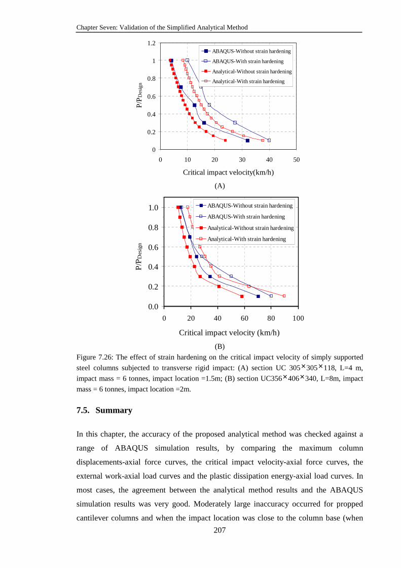
Chapter Seven: Validation of the Simplified Analytical Method
207
0
0.2
0.4
0.6
0.8
1
1.2
0 10 20 30 40 50
Critical impact velocity(km/h)
P/P
Des
ign
ABAQUS-Without strain hardening
ABAQUS-With strain hardening
Analytical-Without strain hardening
Analytical-With strain hardening
(A)
0.0
0.2
0.4
0.6
0.8
1.0
0 20 40 60 80 100
Critical impact velocity (km/h)
P/P
Des
ign
ABAQUS-Without strain hardening
ABAQUS-With strain hardening
Analytical-Without strain hardening
Analytical-With strain hardening
(B)
Figure 7.26: The effect of strain hardening on the critical impact velocity of simply supported
steel columns subjected to transverse rigid impact: (A) section UC 305×305×118, L=4 m,
impact mass = 6 tonnes, impact location =1.5m; (B) section UC356×406×340, L=8m, impact
mass = 6 tonnes, impact location =2m.
7.5. Summary
In this chapter, the accuracy of the proposed analytical method was checked against a
range of ABAQUS simulation results, by comparing the maximum column
displacements-axial force curves, the critical impact velocity-axial force curves, the
external work-axial load curves and the plastic dissipation energy-axial load curves. In
most cases, the agreement between the analytical method results and the ABAQUS
simulation results was very good. Moderately large inaccuracy occurred for propped
cantilever columns and when the impact location was close to the column base (when
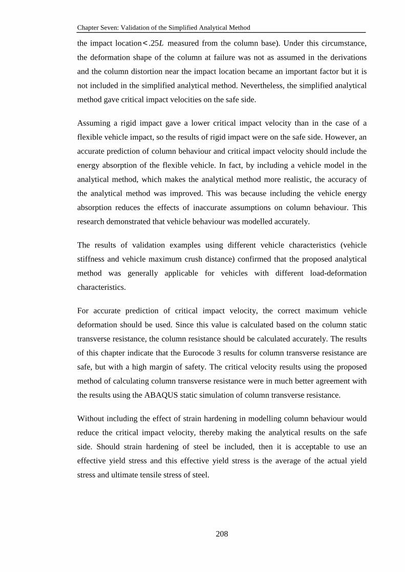
Chapter Seven: Validation of the Simplified Analytical Method
208
the impact location .25L< measured from the column base). Under this circumstance,
the deformation shape of the column at failure was not as assumed in the derivations
and the column distortion near the impact location became an important factor but it is
not included in the simplified analytical method. Nevertheless, the simplified analytical
method gave critical impact velocities on the safe side.
Assuming a rigid impact gave a lower critical impact velocity than in the case of a
flexible vehicle impact, so the results of rigid impact were on the safe side. However, an
accurate prediction of column behaviour and critical impact velocity should include the
energy absorption of the flexible vehicle. In fact, by including a vehicle model in the
analytical method, which makes the analytical method more realistic, the accuracy of
the analytical method was improved. This was because including the vehicle energy
absorption reduces the effects of inaccurate assumptions on column behaviour. This
research demonstrated that vehicle behaviour was modelled accurately.
The results of validation examples using different vehicle characteristics (vehicle
stiffness and vehicle maximum crush distance) confirmed that the proposed analytical
method was generally applicable for vehicles with different load-deformation
characteristics.
For accurate prediction of critical impact velocity, the correct maximum vehicle
deformation should be used. Since this value is calculated based on the column static
transverse resistance, the column resistance should be calculated accurately. The results
of this chapter indicate that the Eurocode 3 results for column transverse resistance are
safe, but with a high margin of safety. The critical velocity results using the proposed
method of calculating column transverse resistance were in much better agreement with
the results using the ABAQUS static simulation of column transverse resistance.
Without including the effect of strain hardening in modelling column behaviour would
reduce the critical impact velocity, thereby making the analytical results on the safe
side. Should strain hardening of steel be included, then it is acceptable to use an
effective yield stress and this effective yield stress is the average of the actual yield
stress and ultimate tensile stress of steel.
Chapter Eight: Assessment of the Current Eurocode 1 Design Methods
209
Chapter Eight
Assessment of the Current Eurocode 1 Design Methods for Steel Columns under Vehicle Impact
8.1. Introduction
In EN 1991 (Eurocode 1) provisions are made for the analysis and design of structures
to resist vehicle impact. The effect of vehicle impact is treated either as an equivalent
static force on the structure as in EN 1991-1-1 (Eurocode1, 2002) or as an approximate
dynamic action as in EN 1991-1-7 (Eurocode1, 2006). This chapter assesses these
requirements and evaluates the applicability of these requirements. In addition, a
possible approach is proposed to improve the accuracy of the design method.
8.2. The equivalent static force approach
The equivalent static force is either calculated using a simple equation (Eurocode1,
2002) or taken as constant values (Eurocode1, 2006, Eurocode1, 2003). Whilst the basis
for the calculation equation is clear, the problem with using this equation is that it is
necessary to obtain the structural and vehicle deformations from other means. This is
not really feasible in design calculations. Otherwise, this design method becomes
redundant. Therefore, this research will not consider this approach any further and will
assess the constant impact forces approach. In section 4.3 of EN 1991-1-7, the
suggested equivalent static forces are 500kN, 700kN and 1000kN respectively for
structural members subjected to transverse vehicle impact in the direction of normal
travel in urban areas, rural areas and on national roads respectively. In addition, sections
4.7.2.1 and 5.6.2.1 of Eurocode 1: Part 2 (Eurocode1, 2003) also gives constant design
values for bridges due to vehicle collision, being 1000kN and 500kN in the parallel and
perpendicular directions of vehicle travel respectively.
To investigate the validity of the equivalent static force assumption in the design of
steel columns subjected to vehicle impact, comparisons between numerical simulation
results and design values were carried out for the four steel column sections shown in
Chapter Eight: Assessment of the Current Eurocode 1 Design Methods
210
Table 8.1. The stress-strain curve of the steel (S355) is assumed to be elastic-perfectly
plastic with a modulus of elasticity of 206×109 N/m2 and a yield stress of 355×106 N/m2.
The validation procedure is as follows:
a. The axial force in the column at which the column fails under vehicle impact at a
certain speed was determined. The simplified numerical vehicle model described
in chapter five was used here to simulate the effect of vehicle impact. Three
impact velocities, 50km/h, 80 km/h and 120 km/h, were considered, representing
speed limits in urban areas, in rural areas and on national roads respectively.
b. Under the same column axial load from (a), the equivalent transverse static force
to cause the column to fail was obtained from a nonlinear static analysis using
ABAQUS. This force was considered to represent the equivalent static design
force corresponding to that of the vehicle impact speed.
Table 8.1: Steel column properties used in the numerical simulations Column
length ( m) Column section
Impact
direction
4 UC 254×254×89 Weak axis
4 UC 305×305×118 Weak axis
4 UC U356×368×202 Weak axis
4 UC U356×406×340 Weak axis
In the static analysis (step b), the lateral force can be applied on the steel column as a
pressure load with the area of application being taken as 250mm×column width for car
collision and 500mm×column width for lorry collisions as suggested in EN 1991-1-7
(Eurocode1, 2002, Ferrer et al., 2010), see Fig. 8.1. The location of the lateral load
application was suggested in the code to be 0.5 m for car collision and 1.5m for lorry
collision. In this research, the vehicle considered was a Chevrolet 1994 Pick-up vehicle.
Since this does not completely match any of the above two vehicle types, the area of
pressure load application was taken as 350mm×column width and the location of impact
was taken as the same as the actual impact location measured in the numerical
simulation model (section 5.3.1.2 in chapter five), which was 0.811m.
Fig. 8.2 compares the equivalent static forces of this research with the design equivalent
static forces suggested by EN 1991-1-7.

Chapter Eight: Assessment of the Current Eurocode 1 Design Methods
211
Figure 8.1: Area of application of the equivalent lateral static load according to EN 1991-1-7 (Eurocode1, 2006)
Figure 8.2: Comparison of equivalent static forces between this research and EN 1991-1-7 design values. It can be seen from Fig. 8.2 that, at the same impact speed, the equivalent static force
values should depend on the column, as represented by the column size. The force
increases as the column size increases. Using a constant value for all column sizes, as in
the current Eurocode 1, is not accurate.
The results in Fig. 8.2 suggest that the values suggested by Eurocode 1 may be
considered acceptable for small and medium sized columns that are commonly used in
buildings of a few storeys high, as represented by the two smaller columns in the figure.
0.0E+00
5.0E+05
1.0E+06
1.5E+06
2.0E+06
2.5E+06
3.0E+06
3.5E+06
4.0E+06
Section254×254×89
Section305×305×118
Section356×368×202
Section356×406×340
Column section size
Equ
ival
ent
sta
tic f
orce
Impact velocity=50km/h
Impact velocity=80km/h
Impact velocity=120km/h
EC1-F=1000kN
EC1-F=700kN EC1-F=500kN
350mm
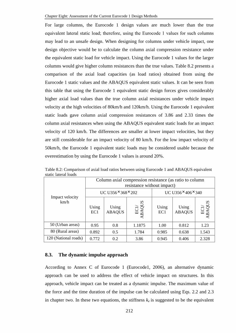
Chapter Eight: Assessment of the Current Eurocode 1 Design Methods
212
For large columns, the Eurocode 1 design values are much lower than the true
equivalent lateral static load; therefore, using the Eurocode 1 values for such columns
may lead to an unsafe design. When designing for columns under vehicle impact, one
design objective would be to calculate the column axial compression resistance under
the equivalent static load for vehicle impact. Using the Eurocode 1 values for the larger
columns would give higher column resistances than the true values. Table 8.2 presents a
comparison of the axial load capacities (as load ratios) obtained from using the
Eurocode 1 static values and the ABAQUS equivalent static values. It can be seen from
this table that using the Eurocode 1 equivalent static design forces gives considerably
higher axial load values than the true column axial resistances under vehicle impact
velocity at the high velocities of 80km/h and 120km/h. Using the Eurocode 1 equivalent
static loads gave column axial compression resistances of 3.86 and 2.33 times the
column axial resistances when using the ABAQUS equivalent static loads for an impact
velocity of 120 km/h. The differences are smaller at lower impact velocities, but they
are still considerable for an impact velocity of 80 km/h. For the low impact velocity of
50km/h, the Eurocode 1 equivalent static loads may be considered usable because the
overestimation by using the Eurocode 1 values is around 20%.
Table 8.2: Comparison of axial load ratios between using Eurocode 1 and ABAQUS equivalent static lateral loads
Impact velocity km/h
Column axial compression resistance (as ratio to column resistance without impact)
UC U356×368×202 UC U356×406×340
Using EC1
Using ABAQUS E
C1/
A
BA
QU
S
Using EC1
Using ABAQUS E
C1/
A
BA
QU
S
50 (Urban areas) 0.95 0.8 1.1875 1.00 0.812 1.23 80 (Rural areas) 0.892 0.5 1.784 0.985 0.638 1.543
120 (National roads) 0.772 0.2 3.86 0.945 0.406 2.328
8.3. The dynamic impulse approach
According to Annex C of Eurocode 1 (Eurocode1, 2006), an alternative dynamic
approach can be used to address the effect of vehicle impact on structures. In this
approach, vehicle impact can be treated as a dynamic impulse. The maximum value of
the force and the time duration of the impulse can be calculated using Eqs. 2.2 and 2.3
in chapter two. In these two equations, the stiffness ke is suggested to be the equivalent

Chapter Eight: Assessment of the Current Eurocode 1 Design Methods
213
elastic stiffness of the impacting object (vehicle) for the case of hard impact or elastic
stiffness of the impacted structure (column) for the case of soft impact. However, the
design code gives no guidance on how to define hard or soft impacts. In fact, results of
the numerical simulations presented in chapters five and seven of this thesis have shown
that, in most cases, both the vehicle and the steel column may experience considerable
deformations during the impact. Therefore, both stiffness terms should be included.
This section will first assess the effects of using either the column or vehicle elastic
stiffness in Eqs. 2.2 and 2.3. Afterwards, it will propose a method of including both
stiffness’ values and assess its accuracy.
A. Using vehicle stiffness
Vehicle stiffness corresponding to each column size can be obtained from the numerical
simulations in chapter five. However, it can also be calculated analytically using the
proposed equation in the same chapter (Eq. 5.14) provided that the required information
about the vehicle crush test on a rigid barrier is available. For the Chevrolet 1994 Pick-
up impacting on a steel column with section size UC 305×305×118, the vehicle
stiffness was 510kN/m (refer to section 5.3.1.2 in chapter five). Therefore, the
equivalent impact impulse can be calculated as follows:
1 510000 1840 30633.3 / sec.r r rF v K M v v kg= ⋅ = × = ×
1/ 1840 / 510000 0.06t M K sec∆ = = =
B. Using column stiffness
To account for the effect of axial compressive force on the column elastic lateral
stiffness, the column stiffness values were calculated from the lateral load-deformation
curves extracted from the nonlinear static simulations conducted in chapter seven (Fig.
7.11).
Alternatively, Eq. 6.42 in chapter six can be used to determine the general equation for
column elastic stiffness taking into account the axial compression load and the location
of the lateral load as follows:
col
Fk
W=
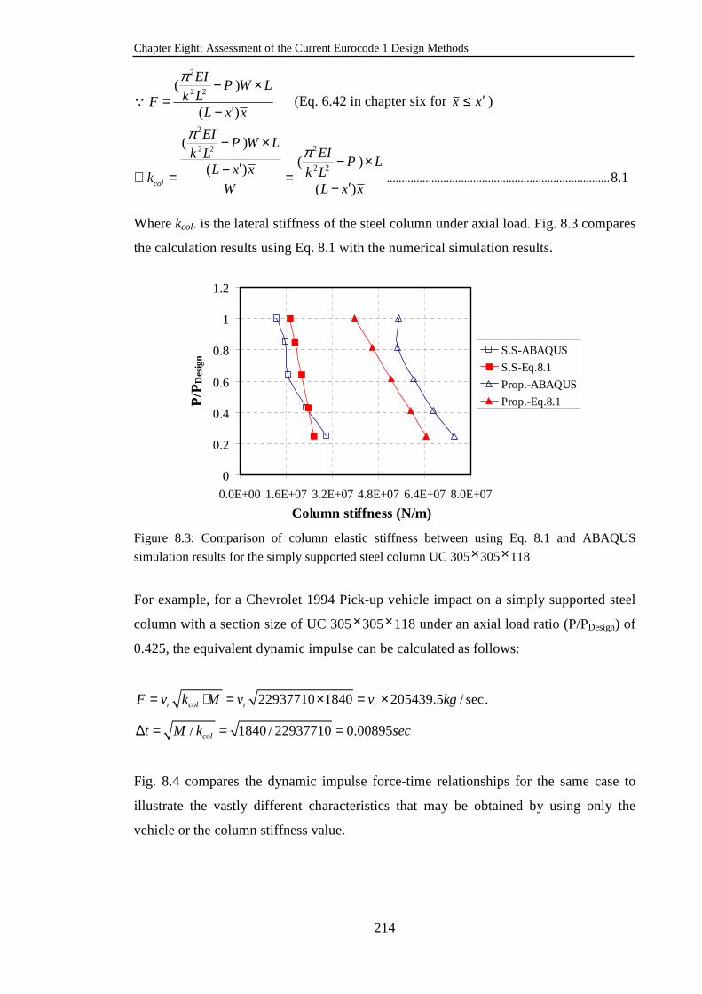
Chapter Eight: Assessment of the Current Eurocode 1 Design Methods
214
∵
2
2 2( )
( )
EIP W L
k LFL x x
π − ×=
′− (Eq. 6.42 in chapter six for xx ′≤ )
2
22 2
2 2
( )( )
( )( )col
EIP W L
EIk LP L
L x x k LkW L x x
ππ
− ×− ×′−∴ = =
′− ........................................................................... 8.1
Where kcol. is the lateral stiffness of the steel column under axial load. Fig. 8.3 compares
the calculation results using Eq. 8.1 with the numerical simulation results.
0
0.2
0.4
0.6
0.8
1
1.2
0.0E+00 1.6E+07 3.2E+07 4.8E+07 6.4E+07 8.0E+07
Column stiffness (N/m)
P/P
Des
ign S.S-ABAQUS
S.S-Eq.8.1
Prop.-ABAQUS
Prop.-Eq.8.1
Figure 8.3: Comparison of column elastic stiffness between using Eq. 8.1 and ABAQUS
simulation results for the simply supported steel column UC 305×305×118
For example, for a Chevrolet 1994 Pick-up vehicle impact on a simply supported steel
column with a section size of UC 305×305×118 under an axial load ratio (P/PDesign) of
0.425, the equivalent dynamic impulse can be calculated as follows:
22937710 1840 205439.5 / sec.r col r rF v k M v v kg= ⋅ = × = ×
/ 1840 / 22937710 0.00895colt M k sec∆ = = =
Fig. 8.4 compares the dynamic impulse force-time relationships for the same case to
illustrate the vastly different characteristics that may be obtained by using only the
vehicle or the column stiffness value.

Chapter Eight: Assessment of the Current Eurocode 1 Design Methods
215
Figure 8.4: Comparison of idealised dynamic impulses by using only the vehicle stiffness or the
column stiffness for column size UC 305×305×118 under impact by a Chevrolet 1994 Pick-up.
The dynamic impulse was applied on the steel column using the AMPLITUDE option
in ABAQUS to determine the critical impact velocity to cause column failure. Figs. 8.5
and 8.6 compare the critical impact velocities from using the dynamic impulses and
from using the vehicle impact simulations in chapter seven.
0.0E+00
4.4E+04
8.8E+04
1.3E+05
1.8E+05
2.2E+05
0.00 0.01 0.03 0.04 0.05 0.07
Time (Sec.)
For
ce (
N)
Using vehicle stiffness
Using column stiffness
30633.3 / sec.rv kg×
205439.5 / secrv kg×
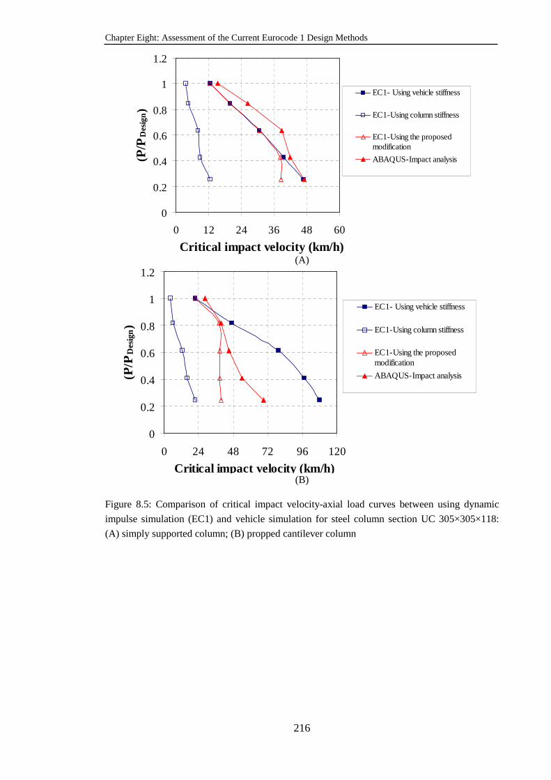
Chapter Eight: Assessment of the Current Eurocode 1 Design Methods
216
0
0.2
0.4
0.6
0.8
1
1.2
0 12 24 36 48 60
Critical impact velocity (km/h)
(P/P
Des
ign)
EC1- Using vehicle stiffness
EC1-Using column stiffness
EC1-Using the proposedmodification
ABAQUS-Impact analysis
(A)
0
0.2
0.4
0.6
0.8
1
1.2
0 24 48 72 96 120
Critical impact velocity (km/h)
(P/P
Des
ign)
EC1- Using vehicle stiffness
EC1-Using column stiffness
EC1-Using the proposedmodification
ABAQUS-Impact analysis
(B)
Figure 8.5: Comparison of critical impact velocity-axial load curves between using dynamic
impulse simulation (EC1) and vehicle simulation for steel column section UC 305×305×118:
(A) simply supported column; (B) propped cantilever column
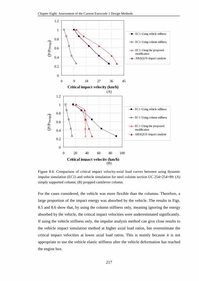
Chapter Eight: Assessment of the Current Eurocode 1 Design Methods
217
0
0.2
0.4
0.6
0.8
1
1.2
0 9 18 27 36 45
Critical impact velocity (km/h)
( P/P
De
sig
n)
EC1-Using vehicle stiffness
EC1-Using column stiffness
EC1-Uisng the proposedmodification
ABAQUS-Impact analysis
(A)
0
0.2
0.4
0.6
0.8
1
1.2
0 20 40 60 80 100
Critical impact velocity (km/h)
( P/P
De
sig
n)
EC1-Using vehicle stiffness
EC1-Using column stiffness
EC1-Uisng the proposedmodification
ABAQUS-Impact analysis
(B)
Figure 8.6: Comparison of critical impact velocity-axial load curves between using dynamic
impulse simulation (EC1) and vehicle simulation for steel column section UC 254×254×89: (A)
simply supported column; (B) propped cantilever column.
For the cases considered, the vehicle was more flexible than the columns. Therefore, a
large proportion of the impact energy was absorbed by the vehicle. The results in Figs.
8.5 and 8.6 show that, by using the column stiffness only, meaning ignoring the energy
absorbed by the vehicle, the critical impact velocities were underestimated significantly.
If using the vehicle stiffness only, the impulse analysis method can give close results to
the vehicle impact simulation method at higher axial load ratios, but overestimate the
critical impact velocities at lower axial load ratios. This is mainly because it is not
appropriate to use the vehicle elastic stiffness after the vehicle deformation has reached
the engine box.
Chapter Eight: Assessment of the Current Eurocode 1 Design Methods
218
After the vehicle deformation has reached the vehicle engine position, the vehicle
becomes rigid and cannot absorb any more impact energy. The following section will
present a modification to take this into consideration.
8.3.1. A proposed modification
According to the assessment results presented in the previous sub-section, it is possible
to use the impulse dynamic analysis method to simulate vehicle impact on columns, but
two modifications should be made. These are explained below.
1-Both the column and the vehicle stiffness should be included when calculating the
impact force. According to energy absorption:
22 2
1 .2 2 2r
col
vF FM
K k+ = ................................................................................................................. 8.2
2- The vehicle energy absorption value reaches the maximum when the vehicle
deformation has reached the engine position. This gives:
2221
max.2 2 2
r
col
K vFC M
k+ = ............................................................................................................ 8.3
Where Cmax is the maximum vehicle deformation before the engine box.
Based on these two modifications, the new impulse can be estimated as in the following
procedure:
(i) The equivalent impact force is first calculated using the equation below (based
on Eq. 8.2):
1 .
1 .
colr
col
M K kF v
K k
⋅ ⋅=+ ................................................................................................................... 8.4
(ii) This gives the impulse duration as:
1 .
1 .
( )col
col
M K kt
K k
⋅ +∆ =⋅ ................................................................................................................ 8.5
(iii) The vehicle deformation, C, can be calculated as follows:
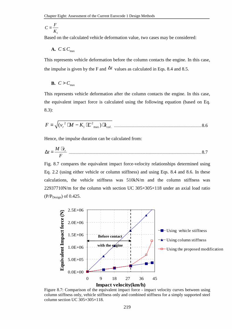
Chapter Eight: Assessment of the Current Eurocode 1 Design Methods
219
1
FC
K=
Based on the calculated vehicle deformation value, two cases may be considered:
A. maxC C≤
This represents vehicle deformation before the column contacts the engine. In this case,
the impulse is given by the F and t∆ values as calculated in Eqs. 8.4 and 8.5.
B. maxC C>
This represents vehicle deformation after the column contacts the engine. In this case,
the equivalent impact force is calculated using the following equation (based on Eq.
8.3):
2 2
1 max .( )r colF v M K C k= ⋅ − ⋅ ⋅ ......................................................................................... 8.6
Hence, the impulse duration can be calculated from:
rM vt
F
⋅∆ = ....................................................................................................................................... 8.7
Fig. 8.7 compares the equivalent impact force-velocity relationships determined using
Eq. 2.2 (using either vehicle or column stiffness) and using Eqs. 8.4 and 8.6. In these
calculations, the vehicle stiffness was 510kN/m and the column stiffness was
22937710N/m for the column with section UC 305×305×118 under an axial load ratio
(P/PDesign) of 0.425.
Figure 8.7: Comparison of the equivalent impact force - impact velocity curves between using column stiffness only, vehicle stiffness only and combined stiffness for a simply supported steel column section UC 305×305×118.
0.0E+00
5.0E+05
1.0E+06
1.5E+06
2.0E+06
2.5E+06
0 9 18 27 36 45
Impact velocity(km/h)
Equ
ivale
nt Im
pact
forc
e (N
)
Using vehicle stiffness
Using column stiffness
Using the proposed modification
Before contact
with the engine

Chapter Eight: Assessment of the Current Eurocode 1 Design Methods
220
Figs 8.5 and 8.6 compare the different critical impact velocity - axial load curves
obtained from the dynamic analyses using the modified impulse calculation method
with using either the vehicle stiffness only or the column stiffness only, and with
ABAQUS vehicle impact analysis.
Because the elastic column stiffness was many times (>30) greater than the vehicle
stiffness, the modified impulse was almost the same as that calculated using the vehicle
stiffness only. Hence, the results in Figs. 8.5 and 8.6 show that when column failure
occurred before the vehicle deformation reached the engine position, the proposed
modification for calculating the impulse gave almost identical results compared with
using the vehicle stiffness only and much better results when compared with using the
column stiffness only.
However, when column failure occurred after the column had made contact with the
vehicle engine and the vehicle should be treated as a rigid body, continuing to use the
vehicle elastic stiffness only for calculating the impulse would mean continued energy
absorption by the vehicle. This would result in overestimation (unsafe) of the critical
impact velocity. Using the modified impulse correctly limited the energy absorption by
the vehicle and produced critical impact velocities that are reasonably close to, and
provide a safe estimation of, the ABAQUS vehicle impact simulation results.
Figs. 8.5 and 8.6 show that the impulse analysis results are not sensitive to the axial load
ratio, particularly when the axial load ratio is low. This is because the impact force was
high and the analysis results were not sensitive to the time duration of the impulse
(Thilakarathna et al., 2010). Nevertheless, using the proposed modification for impulse
made a huge improvement to the critical velocity results compared with using only
either the vehicle or column stiffness.
In summary, using the proposed method of calculating the dynamic impulse eliminated
the gross errors of using either the column stiffness only or the vehicle stiffness only.
Although using the impulse-based dynamic analysis still resulted in some errors,
particularly when the applied axial loads were low, the dynamic analysis results may be
considered acceptable.
Chapter Eight: Assessment of the Current Eurocode 1 Design Methods
221
8.4. Summary
This chapter has presented a detailed assessment of the design requirements suggested
by Eurocode 1 regarding the design of steel columns to resist vehicle impact. Both the
static and dynamic approaches in Eurocode1 have been evaluated. From the detailed
comparisons between the design results and the ABAQUS impact simulation results, the
following conclusions may be drawn:
(1) the equivalent static design forces may be considered acceptable for column design
if the column section sizes are moderate, as used in typical multi-storey buildings of
no more than 10 storeys. If the column sizes are greater, using the Eurocode 1
equivalent static forces will overestimate the axial compression resistance of the
columns especially when the columns are used in structures located in rural areas or
near national roads with high vehicle speeds. However, if the vehicle velocities are
low (<50 km/h), the Eurocode 1 equivalent static forces may still be used.
(2) Using a dynamic impulse to represent the dynamic action of vehicle impact is a
reasonable approximation. However, when calculating the force, it is not appropriate
to use only either the column elastic stiffness or the vehicle elastic stiffness, as
recommended by Eurocode 1. It is necessary to include both the column and vehicle
stiffness values. Furthermore, vehicle behaviour should be divided into two stages,
before the column is in contact with the vehicle engine and after contact. After the
column is in contact with the vehicle engine, the energy absorbed by the vehicle
should be limited by the maximum deformation of the vehicle. In this chapter, a
modification has been suggested for calculating the dynamic impulse of vehicle
impact. Using this modified dynamic impulse in dynamic analysis was able to
eliminate the gross errors caused by using only the vehicle stiffness or the column
stiffness and produced results of critical vehicle velocity that are close to the
ABAQUS vehicle impact simulation results.
Chapter Nine: Conclusions and Recommendations
222
Chapter Nine
Conclusions and Recommendations for Future Research
Studies
9.1. Introduction
This thesis has presented, in detail, the work undertaken by the author in a PhD research
programme to investigate the behaviour of axially compressed steel columns under
vehicle impact. The ultimate aim of the research was to gain a thorough understanding
of the aforementioned problem and to develop an efficient, accurate and robust design
approach. This research included the following research work packages: numerical
modelling using ABAQUS/Explicit, a parametric study of steel column behaviour under
transverse impact, development of a simplified vehicle model, development of an
analytical method for column response under transverse impact and an assessment of
the current design provisions.
This chapter will summarise the main findings of the study in each of these packages
and provides recommendations for future research studies to improve or extend the
current work.
9.2. Conclusions of this research
The following conclusions can be extracted from the following research tasks:
9.2.1. Numerical modelling of steel column behaviour under transverse
impact
a. The results presented in this thesis can be considered to have provided an extensive
body of evidence that the finite element code ABAQUS/Explicit is capable of
modelling axially loaded steel columns under transverse impact provided that the
associated geometrical, material and contact modelling parameters are selected and
implemented correctly as presented in this study. Based on the validation results
presented in this thesis, using first order (linear) three dimensional solid or shell
Chapter Nine: Conclusions and Recommendations
223
elements with reduced integration and hourglass control is suitable. An isotropic
classical metal plasticity model in connection with the progressive damage and
failure model available in ABAQUS/Explicit can be used to simulate the behavior
and all possible failure modes of the steel columns subjected to transverse impact.
Contact interaction between the impacting body and the steel column can be
simulated using either the contact pair algorithm or the general contact algorithm
available in ABAQUS/Explicit, depending on the type of surfaces involved in the
contact, with hard and penalty friction formulations to describe the mechanical
properties in the normal and tangential directions respectively.
b. It has been proven numerically that damping has only a minor effect on the
response and contact force of pre-compressed columns subjected to transverse
impact load.
9.2.2. Behaviour and failure modes of steel columns under transverse impact
a. Global buckling is the predominant failure mode for axially unrestrained compressed
steel columns under transverse impact. Some column failure may involve large
local flange distortion at, and around, the impact area. However, detailed
inspections of the column behaviour at failure simulated in this study have revealed
that the flange local distortion is a result, not the cause, of column global failure.
b. The value of the kinetic energy of the impact is the key factor in determining the
column’s global failure. At the same impact kinetic energy, different values of
impacting mass and velocity have a minor effect on column failure.
c. Except at very low levels of axial compressive loads (<25% design resistance), the
formation of the plastic hinge within the column length is almost independent of the
impact position, with the plastic hinge location being close to the centre of the
column.
d. The most critical direction of impact is that which causes bending of the column
about the minor axis.
e. Damping can be neglected when calculating the critical impact velocity because of
its minor effects on column behaviour and failure.
Chapter Nine: Conclusions and Recommendations
224
f. Both strain hardening and strain rate have beneficial effects on column critical
impact velocity. While it is important to include the effect of strain hardening in the
development of a simplified method, the effect of strain rate can be discarded safely
because of the relatively low influence of this effect.
9.2.3. Simplified vehicle model
a. It is not appropriate to assume vehicles as rigid impactors when studying the
behaviour of columns under vehicle impact.
b. The impacting vehicle can be simplified as a spring mass system with the linear
spring representing the stiffness characteristics of the vehicle. The spring force -
deformation relationship is assumed to be bilinear, with the first part representing
the vehicle deformation behaviour up to the engine box and the second part
representing the stiffness of the engine box, which can be assumed to be rigid.
c. The current study has presented a method to obtain the stiffness value of a vehicle
before reaching the engine box. This method is based on using the method originally
suggested by Campbell to obtain the vehicle force - deformation relationship per unit
width and integrating this force - deformation relationship over the deformation
profile of the vehicle after impact on a column with a finite width. Comparison
between the vehicle stiffness values derived in such a way and those extracted from
the corresponding numerical simulations indicates that the difference is less than
25% for different column section sizes.
9.2.4. Development of an analytical method for column behaviour under
transverse impact.
a. A quasi-static response for an impacted steel column can be assumed when
conducting an energy balance analysis of the vehicle-column system. The energy
absorbed by the column is by elastic deformation and plastic hinge rotation at the
plastic hinge locations. It is important to include the work undertaken by the axial
force in the column due to column shortening when undergoing lateral deformation.
Column global plastic buckling occurs when the column plastic hinge mechanism
loses equilibrium under an axial compressive force in a deformed state. The final
column equilibrium position determines the maximum plastic hinge rotations.
Chapter Nine: Conclusions and Recommendations
225
b. To calculate the energy absorbed by the vehicle, the maximum deformation of the
vehicle frontal structure is determined based on the maximum transverse static
resistance of the column. The Eurocode 3 method to obtain the column transverse
static resistance under the influence of an axial load is overly conservative. An
alternative column transverse static resistance – axial force relationship has been
proposed.
c. To include the effect of strain hardening, the average of the steel yield stress and
ultimate tensile stress can be approximately used in the elastic-perfectly-plastic
representation of the steel stress-strain relationship.
9.2.5. Assessment of current design methods in Eurocode 1
a. The equivalent static design force approach can be used in the design of steel
columns with moderate sizes which are typically used in low multi-storey buildings
of no more than 10 storeys. For bigger sizes of columns, this study has shown that
it is unsafe to use the Eurocode 1 equivalent static forces especially when the
columns are used in structures located in rural areas or near national roads when the
vehicle velocity exceeds 80 km/h.
b. It is acceptable to use dynamic impulse to represent the dynamic action of vehicle
impact in a dynamic analysis. However, it is not appropriate to use only either the
column elastic stiffness or the vehicle elastic stiffness to calculate the equivalent
impulse force as recommended by Eurocode 1. Instead, it is necessary to include
both the column and vehicle stiffness values with the vehicle behaviour divided into
two stages: before, and after, the column is in contact with the vehicle engine.
9.3. Recommendations for future research works
Since this research is amongst the first in the numerical and analytical studies of the
behaviour of axially loaded steel columns subjected to vehicle impact, it was not
possible to cover all aspects of the problem. A number of further research studies can be
pursued to improve the knowledge and understanding in this area:
1. The present study has focused on the behaviour of H section steel columns under
vehicle impact. The behaviour of other section shapes should be investigated. In
addition, the study can also be developed to consider other types of columns including
Chapter Nine: Conclusions and Recommendations
226
reinforced concrete columns, pre-stressed concrete columns and concrete filled steel
columns.
2. The numerical simulations carried out in this study have utilized solid elements to
model the steel column. Although using solid elements gives more accurate results, it
requires a large amount of computation time. Using line (beam) elements will be much
more efficient, particularly as a tool for practical design. It would, however, be
necessary to check the accuracy of using more simplified simulation methods.
3. The current study has focused on vehicle impact in the direction that would cause
column bending about the weak axis of the column, this being considered as the most
critical direction of impact. Further research studies could investigate in more detail the
behaviour of column behaviour under impact in other directions.
4. In this study, the steel column is subjected to pure axial compression without any
bending moment. The effects of combined axial compression and bending moment
should be investigated.
5. In the present study, the effect of vehicle impact on the behaviour and failure modes
of steel columns has been studied by investigating the impact behaviour of an isolated
column. Since the context of this research is structural robustness under extreme
loading, further research studies should be carried out to investigate the effect of whole
structures.
6. Because of its availability, the presented study has used the numerical model of a
Chevrolet C2500 1994 Pick-up vehicle to validate the proposed simplified numerical
vehicle model. Further research studies can be carried out to investigate whether the
proposed simplified vehicle model can be applied to other types of vehicles.
7. In the simplified analytical method, the moment-rotation curve of the plastic hinge
formed in the column is assumed to be elastic-perfectly plastic. For refinement of the
analytical model, more realistic moment-rotation curves (considering elastic-plastic
behaviour and strain hardening behaviour) should be investigated.
8. The analytical model has been developed based on the assumption of column failure
by global buckling. The effects of energy absorption in the column through local

Chapter Nine: Conclusions and Recommendations
227
deformations in the impact zone should be investigated. In addition, the energy
absorbed by shear deformation in the column may have some effect, particularly when
the impact location is very close to the column base. This should be researched.
9. It is expected that the conclusions of this research can be applied to columns under
impact from other sources, such as cranes, rocks and flying debris. Further research
studies may be undertaken to assess the applicability of the proposed method of analysis
in such cases.
References
228
References
BS 5950-1:2000, British Standard- Structural use of steelwork in building — Part 1: Code of practice for design — Rolled and welded sections, Incorporating Corrigenda Nos. 1 and 2 and Amendment No. 1. AASHTO 2007. LRFD bridge design specifications. merican Association of State Highway and Transportation Officials. Washington, D.C, USA. ACI 1992. Analysis and design of reinforced and prestressed-concrete guideway structures. Reported by ACI Committee 358. ADACHI, T., TANAKA, T., SASTRANEGARA, A., YAMAJI, A., KIM, S.-K. & YANG, I.-Y. 2004. Effect of transverse impact on buckling behavior of a column under static axial compressive force. International Journal of Impact Engineering, 30, 465-475. B. MILNER, R.H. GRZEBIETA & ZOU, R. 2001. Theoretical Study of a Vehicle-Pole Impact. Proceedings Road Safety Research, Policing and Education Conference, CMO Monash University, ISBN 0-7326-2190-9, Melbourne. BAI, Y. & PEDERSEN, P. T. 1993. Elastic-plastic behaviour of offshore steel structures under impact loads. International Journal of Impact Engineering, 13, 99-115. BAMBACH, M. R. 2011. Design of hollow and concrete filled steel and stainless steel tubular columns for transverse impact loads. Thin-Walled Structures, 49, 1251–1260. BAMBACH, M. R., JAMA, H., ZHAO, X. L. & GRZEBIETA, R. H. 2008. Hollow and concrete filled steel hollow sections under transverse impact loads. Engineering Structures, 30, 2859-2870. BELYTSCHKO, T., MORAN, B. & W. K. LIU 2000. Nonlinear finite elements for continua and structures, John Wiley. BIGGS, J. M. 1964. Introduction to Structural Dynamics. McGraw-Hill, New York, BOH, J. W., LOUCA, L. A. & CHOO, Y. S. 2004. Strain rate effects on the response of stainless steel corrugated firewalls subjected to hydrocarbon explosions. Journal of Constructional Steel Research, 60, 1–29. BONET, J. & WOOD, R. D. 1997. Nonlinear Continuum Mechanics for Finite Element Analysis. Cambridge. BRELL, E. 2005. Simplified models of vehicle impact for injury mitigation PhD Queensland University of Technology BS 2001. Structural use of steelwork in building Part 1:code of practice for design - rolled and welded sections. London: British Standards Institution.
References
229
CAMPBELL, K. E. 1976. Energy basis for collision severity. Environmental Activities Staff,United States: General Motors Corp, SAE paper 740565. CHEN, F. L. & YU, T. X. 2000. Influence of Axial Pre-Load on Plastic Failure of Beams Subjected to Transverse Dynamic Load. Key Engineering Materials, (117-180), 255-260. CLOUGH, R. W. & PENZIEN, J. 1975. Dynamics of Structures. McGraw-Hill. COWPER , G. R. & SYMONDS, P. S. 1957. Strain hardening and strain rate effects in the impact loading of cantilever beams Brown University Division of Applied Mathematics Report September CRISFIELD, M. A. 1997. Non-linear finite element analysis of solids and structures; Vol.2, Advanced topics, Wiley. DOROGOY, A. & RITTEL, D. 2008. Transverse impact of free-free square aluminum beams: An experimental-numerical investigation. International Journal of Impact Engineering, 35, 569-577. DUAN, L. & CHEN, W. F. 1990. A Yield Surface Equation For Doubly Symmetrical Sections. Eng. Stru, 12, 112-114. EL-TAWIL, S., SEVERINO, E. & FONSECA, P. 2005. Vehicle collision with bridge piers. Journal of Bridge Engineering, 10, 345–353. ELLIS, B. R. 2003. Road vehicle impacts on buildings in the uk - Regulation and risk. The structural engineer, 81, 36-40. ELMARAKBI, A., SENNAH, K., SAMAAN, M. & SIRIYA, P. 2006. Crashworthiness of Motor Vehicle and Traffic Light Pole in Frontal Collisions. The ASCE JOURNAL OF TRANSPORTATION ENGINEERING, 132(9), 722-733. EMORI, R. I. 1968. Analytical approach to Automobile Collisions. Society of automative engineers, automative engineering congress, SAE paper 680016. EUROCODE1 2002. BS EN 1991-1-1-:2002, Eurocode 1: Actions on structures — Part 1-1: General actions — Densities, self-weight, imposed loads for buildings- (ANNEX B), Incorporating corrigenda December 2004 and March 2009. EUROCODE1 2003. BS EN 1991-2:2003, Eurocode 1: Actions on structures — Part 2: Traffic loads on bridges, Incorporating Corrigenda, December 2004 and February 2010. EUROCODE1 2006. BS EN 1991-1-7:2006, Eurocode 1 — Actions on structures —Part 1-7: General actions — Accidental actions, Incorporating corrigendum February 2010. EUROCODE3 2005. BS EN 1993-1-1:2005, Eurocode 3 — Design of steel structures —Part 1-1:General rules and rules for buildings, Incorporating Corrigenda February 2006 and April 2009.

References
230
FERRER, B., IVORRA, S., SEGOVIA, E. & IRLES, R. 2010. Tridimensional modelization of the impact of a vehicle against a metallic parking column at a low speed. Engineering Structures, 32, 1986-1992. GHOSE, A. 2009. Strategies for the management of bridges for vehicular impacts. Structures and Buildings, 162, 3-10. HIGHWAYS AGENCY 2004. The Design of Highway Bridges for Vehicle Collision Loads. Highways Agency. Design Manual For Roads And Bridges, Vol. 1, Sec. 3, Part 5, BD 60/04 , London HUMAR, L. J. 2002. Dynamics of Structures,2nd., Lisse ; Abingdon : A.A. Balkema 2002. JIANG, T., GRZEBIETA, R. H. & ZHAO, X. L. 2004. Predicting impact loads of a car crashing into a concrete roadside safety barrier. International Journal of Crashworthiness, 9, 45-63. JOHNSON, K. L. 1985. Contact Mechanics. Cambridge. JOHNSON, W. 1972. Impact Strength of Material. 250-280. JONES, N. 1995. Quasi-static analysis of structural impact damage. Journal of Constructional Steel Research, 33, 151-177. JONES, N. 1997. Structural Impact Cambridge University Press, UK. KAMAL, M. M. 1970. Analysis and simulation of Vehicle to Barrier Impact International Automobile Safety Conference SAE Paper No.700414. KLYAVIN, O., MICHAILOV, A. & BOROVKOV, A. 2008. Finite Element Modeling of the Crash-Tests for Energy Absorbing Lighting Columns. ENOC-2008, Saint Petersburg, Russia, June, 30–July, 4 LIN, K. H. 1973. A rear- end barrier impqct simulation model for unibody passenger cars SAE Trans., 82. LIU, J. & JONES, N. 1987. Experimental investigation of clamped beams struck transversely by a mass. International Journal of Impact Engineering, 6, 303-335. LIU, J. & JONES, N. 1988. Dynamic response and failure of a rigid plastic clamped beam struck by a mass at any point on the span. International Journal of Solids and Structures, 24, 251–70. MANNAN, M. N., ANSARI, R. & ABBAS, H. 2008. Failure of aluminium beams under low velocity impact. International Journal of Impact Engineering, 35, 1201-1212. MENKES, S. B. & OPAT, H. J. 1973. Broken beams. Experimental Mechanics, 13, 480-486
References
231
MILNER, B., GRZEBIETA, R. H. & ZOU, R. 2001. Theoretical Study of a Vehicle-Pole Impact. Proceedings Road Safety Research, Policing and Education Conference, CMO Monash University, ISBN 0-7326-2190-9, Melbourne. NCAC. 2011. Available: http://www.ncac.gwu.edu/vml/models.html, 1/ 08/2012. NHTSA. 2011. Available: http://www.nhtsa.gov/Research/Databases+and+Software, 1/ 08/2012. NONAKA, T. 1967. Some interaction effects in a problem of plastic beam dynamics, parts 1–3. Journal of Applied Mechanics, 34, 623–43. PARKES, E. W. 1958. The permanent deformation of an encastre beam struck transversely at any point in its span. Proc. Instn Civ. Engrs, 10, 227–304. QIAO, J. S., CHEN, J. H. & CHE, H. Y. 2006. Crashworthiness assessment of square aluminum extrusions considering the damage evolution. Thin-Walled Structures, 44, 692-700. SAMUELIDES, E. & FRIEZE, P. A. 1984. Analytical and Numerical Simulation of Beams Subjected to Impact Structural Impact and Crashworthiness, Vol.2, 355-368. SASTRANEGARA, A., ADACHI, T. & YAMAJI, A. 2005. Improving energy absorption of impacted column due to transverse impact: A finite element analysis. International Journal of Impact Engineering, 32, 444-460. SASTRANEGARA, A., ADACHI, T. & YAMAJI, A. 2006. Effect of transverse impact on buckling behavior of compressed column. Thin-Walled Structures, 44, 701-707. SHARMA, H., HURLEBAUS, S. & GARDONI, P. 2012. Performance-based response evaluation of reinforced concrete columns subject to vehicle impact. International Journal of Impact Engineering 43, 52-62 SHEN, W. Q. & JONES, N. 1991. A comment on the low speed impact of a clamped beam by a heavy-striker. Mechanics. Structures and Machines, 19, 527-49. SHOPE, R. L. 2006. Response Of Wide Flange Steel Columns Subjected To Constant Axial Load And Lateral Blast Load (PhD )Thesis. SIDDALL, D. & DAY, T. 1996. Updating the Vehicle Class Categories. SAE Technical Paper 960897, doi:10.4271/960897 SIMULIA 2010a. Analysis user’s manual, Vo. 3 (Material), Providence, Rhode Island, USA., SIMULIA, Dassault Systèmes. SIMULIA 2010b. Analysis user’s manual, Vo. 4 ( Elements), Providence, Rhode Island, USA., SIMULIA, Dassault Systèmes. SIMULIA 2010c. Analysis user’s manual, Vol. 1 (Introduction, Spatial Modeling, Execution & Output), Providence, Rhode Island, USA., SIMULIA, Dassault Systèmes.
References
232
SIMULIA 2010d. Analysis user’s manual, Vol. 2 (Analysis), Providence, Rhode Island, USA., SIMULIA, Dassault Systèmes. SIMULIA 2010e. Analysis user’s manual, Vol. 5 (Prescribed Conditions, Constraints & Interactions.), Providence, Rhode Island, USA., SIMULIA, Dassault Systèmes. SIMULIA 2010f. Getting Started with Abaqus: Interactive Edition, Providence, Rhode Island, USA., SIMULIA, Dassault Systèmes. SYMONDS, P. & JONES, N. 1972. Impulsive loading of fully clamped beams with finite plastic deflections and strain-rate sensitivity. International Journal of Mechanical Sciences, 14, 49–69. SYMONDS, P. & MENTEL, T. 1958. Impulsive loading of plastic beams with axial constraints. Journal of the Mechanics and Physics of Solids, 6, 186–202. TANI, M. & EMORI, R. I. 1970. A study on automobile crashworthness. Society of automative engineers, automative engineering congress, SAE paper 700175. THILAKARATHNA, H. M. I., THAMBIRATNAM, D. P., DHANA SEKAR, M. & PERERA, N. 2010. Numerical simulation of axially loaded concrete columns under transverse impact and vulnerability assessment. International Journal of Impact Engineering, 37, 1100-1112 TIMOSHENKO, S. P., GERE, J. M. 1961. Theory of Elastic Stability. 2nd ed. McGraw-Hill, NY. TSANG, H.-H. & LAM, N. T. K. 2008. Collapse of Reinforced Concrete Column by Vehicle Impact. Computer-Aided Civil and Infrastructure Engineering, 23, 427-436. VARAT, M. & HUSHER, S. 2000 Vehicle impact response analysis through the use of accelerometer data. SAE Technical Paper Series, Detroit, Michigan. VROUWENVELDER, T. 2000. Stochastic modelling of extreme action events in structural engineering. Probabilistic Engineering Mechanics, 15, 109-117. WAGSTROM, L., THOMSON, R. & PIPKORN, B. 2004. Structural adaptivity for acceleration level reduction in passenger car frontal collisions. International Journal of Crashworthiness, 9, 121–27. WEN, H. M., REDDY, T. Y. & REID, S. R. 1995. Deformation and failure of clamped beams under low speed impact loading. International Journal of Impact Engineering, 16, 435-454. WONG, M. B. 2009. Elastic Analysis and Design of Steel Structures, 1st Edition. YU, J.-L. & JONES, N. 1997. Numerical simulation of impact loaded steel beams and the failure criteria. International Journal of Solids and Structures, 34, 3977-4004. YU, J. & JONES, N. 1989. Numerical simulation of a clamped beam under impact loading. Computers & Structures, 32, 281-293.

References
233
YU, J. & JONES, N. 1991. Further experimental investigations on the failure of clamped beams under impact loads. International Journal of Solids and Structures, 27, 1113-1137. ZAOUK, A. K., BEDEWI, N. E., KAN, C.-D. & MARZOUGUI, D. 1996. Validation of a non-linear finite element vehicle model using multiple impact data. Crashworthiness and occupant protection in transportation systems, Vol. 218, 91-106. ZEINODDINI, M., HARDING, J. E. & PARKE, G. A. R. 2008a. Axially pre-loaded steel tubes subjected to lateral impacts (a numerical simulation)c. International Journal of Impact Engineering, 35, 1267-1279. ZEINODDINI, M., PARKE, G. A. R. & HARDING, J. E. 2002. Axially pre-loaded steel tubes subjected to lateral impacts: an experimental study. International Journal of Impact Engineering, 27, 669-690. ZEINODDINI, M., PARKE, G. A. R. & HARDING, J. E. 2008b. Interface Forces in Laterally Impacted Steel Tubes. Experimental Mechanics, 48, 265–280 ZIENKIEWICZ, O. C. & TAYLOR, R. L. 1991. The finite element method, Vol.2, Solid and fluid mechanics: dynamics and non-linearity, London, McGraw-Hill 4th ed.
Appendix A: Publications
234
Appendix A
Publications
The following papers were extracted from this study:
A. Published papers:
[1]. AL-THAIRY, H. & WANG, Y. C. 2011. A numerical study of the behaviour
and failure modes of axially compressed steel columns subjected to transverse impact. International Journal of Impact Engineering, 38, 732-744. http://dx.doi.org/10.1016/j.ijimpeng.2011.03.00
[2]. AL-THAIRY, H. & WANG, Y. C. 2010. Numerical and Analytical Study of
Behavior of Axially Loaded Steel Columns Subjected to Transverse Impact. 4th International Conference on Steel & Composite Structures (ICSCS). Sydney, Australia: Research Publishing Services.
B. Submitted papers:
[1]. AL-THAIRY, H. & WANG, Y. C. 2011. A Simplified Analytical Method for
Predicting the Critical Velocity of Transverse Rigid Body Impact on Steel Columns International Journal of Impact Engineering, Submitted in July 2011.
[2]. AL-THAIRY, H. & WANG, Y. C. 2011. Simplified FE vehicle model for assessing the vulnerability of axially compressed steel columns against vehicle frontal impact. Journal of Constructional Steel Research, Submitted in June 2012.
[3]. AL-THAIRY, H. & WANG, Y. C. 2012. An Assessment of the Current
Eurocode 1 Design Methods for Building Structure Steel Columns under Vehicle Impact. Journal of Constructional Steel Research, Submitted in July 2012.