all point correlation functions in syk … the six-point function involves gluing together three...
TRANSCRIPT
All point correlation functions in SYK
David J. Gross and Vladimir Rosenhaus
Kavli Institute for Theoretical Physics
University of California, Santa Barbara, CA 93106
Large N melonic theories are characterized by two-point function Feynman diagrams built
exclusively out of melons. This leads to conformal invariance at strong coupling, four-point
function diagrams that are exclusively ladders, and higher-point functions that are built out of
four-point functions joined together. We uncover an incredibly useful property of these theories:
the six-point function, or equivalently, the three-point function of the primary O(N) invariant
bilinears, regarded as an analytic function of the operator dimensions, fully determines all cor-
relation functions, to leading nontrivial order in 1/N , through simple Feynman-like rules. The
result is applicable to any theory, not necessarily melonic, in which higher-point correlators are
built out of four-point functions. We explicitly calculate the bilinear three-point function for
q-body SYK, at any q. This leads to the bilinear four-point function, as well as all higher-point
functions, expressed in terms of higher-point conformal blocks, which we discuss. We find uni-
versality of correlators of operators of large dimension, which we simplify through a saddle point
analysis. We comment on the implications for the AdS dual of SYK.
arX
iv:1
710.
0811
3v2
[he
p-th
] 1
9 D
ec 2
017
Contents
1. Introduction 2
1.1. Outline of computation . . . . . . . . . . . . . . . . . . . . . . . . . . . . . . . . 3
2. SYK Ladders 6
2.1. SYK basics . . . . . . . . . . . . . . . . . . . . . . . . . . . . . . . . . . . . . . 6
2.2. Fermion four-point function: summing ladders . . . . . . . . . . . . . . . . . . . 8
3. Bilinear Three-Point Function 13
3.1. Contact diagrams . . . . . . . . . . . . . . . . . . . . . . . . . . . . . . . . . . . 14
3.2. Planar diagrams . . . . . . . . . . . . . . . . . . . . . . . . . . . . . . . . . . . . 15
4. Bilinear Four-Point Function 20
4.1. Cutting melons and 2p-point functions . . . . . . . . . . . . . . . . . . . . . . . 20
4.2. Outline . . . . . . . . . . . . . . . . . . . . . . . . . . . . . . . . . . . . . . . . . 21
4.3. Splitting and recombining conformal blocks . . . . . . . . . . . . . . . . . . . . . 22
4.4. Combining ingredients and comments . . . . . . . . . . . . . . . . . . . . . . . . 25
5. Higher-Point Correlation Functions 29
5.1. Five-point conformal blocks . . . . . . . . . . . . . . . . . . . . . . . . . . . . . 30
6. Generalized Free Field Theory 32
6.1. Wick contractions and generating function . . . . . . . . . . . . . . . . . . . . . 32
6.2. Asymptotic three-point function . . . . . . . . . . . . . . . . . . . . . . . . . . . 35
6.3. Asymptotic four-point function . . . . . . . . . . . . . . . . . . . . . . . . . . . 37
7. Bulk 41
7.1. Constructing the bulk . . . . . . . . . . . . . . . . . . . . . . . . . . . . . . . . 41
7.2. Preliminaries . . . . . . . . . . . . . . . . . . . . . . . . . . . . . . . . . . . . . 43
7.3. Exchange Witten diagrams . . . . . . . . . . . . . . . . . . . . . . . . . . . . . . 45
8. Discussion 47
A. Conformal Blocks 48
A.1. Mellin space . . . . . . . . . . . . . . . . . . . . . . . . . . . . . . . . . . . . . . 51
B. Large q Limit 52
1

C. Free Field Theory 55
D. Fermion Correlation Functions 56
E. Contact Diagrams 58
F. Witten Diagrams 59
G. An AdS2 Brane in AdS3 62
1. Introduction
Strongly coupled quantum field theories are often prohibitively difficult to study, yet, in the
rare cases that one succeeds, they reveal a wealth of phenomena. This has been evidenced over
the past decade with the remarkable integrability results in maximally supersymmetric N = 4
Yang-Mills [1]. The integrability of N = 4 implies that the theory is, in principle, solvable at
large N . However, in practice the solution is neither simple nor direct. Like any matrix model,
the large N dominant Feynman diagrams are planar, and there are no known general techniques
to sum planar diagrams. It would be incredibly useful to have simpler large N models, with
diagrammatic structures that allow for full summation.
Melonic models are of this type. These have arisen in a number of independent contexts,
including: models of Bose fluids [2], models of spin glasses [3], and tensor models [4]. The specific
theory we will focus on is the SYK model [5]: a 0 + 1 dimensional model of Majorana fermions
with q-body interactions. Through a simple extension, our results are applicable to any melonic
theory. In fact, as we will discuss later, our results extend to an even broader class of theories,
provided they have the diagrammatic structure that higher-point correlators are built out of
four-point functions. In this paper we solve SYK: we give expressions for the connected piece of
the fermion 2p-point correlation function, for any p, to leading nontrivial order in 1/N .
What are the features of melonic theories that make them solvable? At the level of the two-
point function, it is the fact that, at leading order in 1/N , all Feynman diagrams are iterations
of melons nested within melons. This self-similarity leads to an integral equation determining
the two-point function, which in turn has a conformal solution at strong coupling. At the level
of the four-point function, all leading large N Feynman diagrams are ladders, with an arbitrary
number of rungs: summing all ladder diagrams is no more difficult than summing a geometric
series, provided one uses the appropriate basis.
The focus of this paper is the six-point function, and higher. As input, we need to know the
2
+=
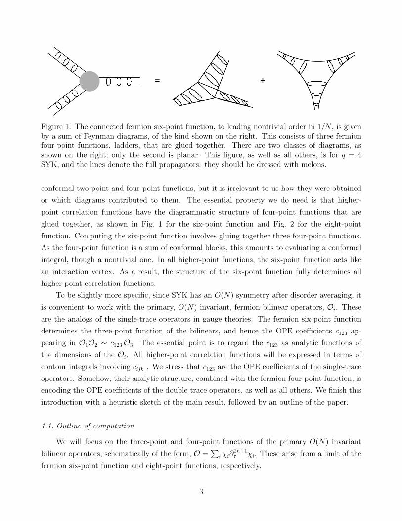
Figure 1: The connected fermion six-point function, to leading nontrivial order in 1/N , is givenby a sum of Feynman diagrams, of the kind shown on the right. This consists of three fermionfour-point functions, ladders, that are glued together. There are two classes of diagrams, asshown on the right; only the second is planar. This figure, as well as all others, is for q = 4SYK, and the lines denote the full propagators: they should be dressed with melons.
conformal two-point and four-point functions, but it is irrelevant to us how they were obtained
or which diagrams contributed to them. The essential property we do need is that higher-
point correlation functions have the diagrammatic structure of four-point functions that are
glued together, as shown in Fig. 1 for the six-point function and Fig. 2 for the eight-point
function. Computing the six-point function involves gluing together three four-point functions.
As the four-point function is a sum of conformal blocks, this amounts to evaluating a conformal
integral, though a nontrivial one. In all higher-point functions, the six-point function acts like
an interaction vertex. As a result, the structure of the six-point function fully determines all
higher-point correlation functions.
To be slightly more specific, since SYK has an O(N) symmetry after disorder averaging, it
is convenient to work with the primary, O(N) invariant, fermion bilinear operators, Oi. These
are the analogs of the single-trace operators in gauge theories. The fermion six-point function
determines the three-point function of the bilinears, and hence the OPE coefficients c123 ap-
pearing in O1O2 ∼ c123O3. The essential point is to regard the c123 as analytic functions of
the dimensions of the Oi. All higher-point correlation functions will be expressed in terms of
contour integrals involving cijk . We stress that c123 are the OPE coefficients of the single-trace
operators. Somehow, their analytic structure, combined with the fermion four-point function, is
encoding the OPE coefficients of the double-trace operators, as well as all others. We finish this
introduction with a heuristic sketch of the main result, followed by an outline of the paper.
1.1. Outline of computation
We will focus on the three-point and four-point functions of the primary O(N) invariant
bilinear operators, schematically of the form, O =∑
i χi∂2n+1τ χi. These arise from a limit of the
fermion six-point function and eight-point functions, respectively.
3
1
2
3
4
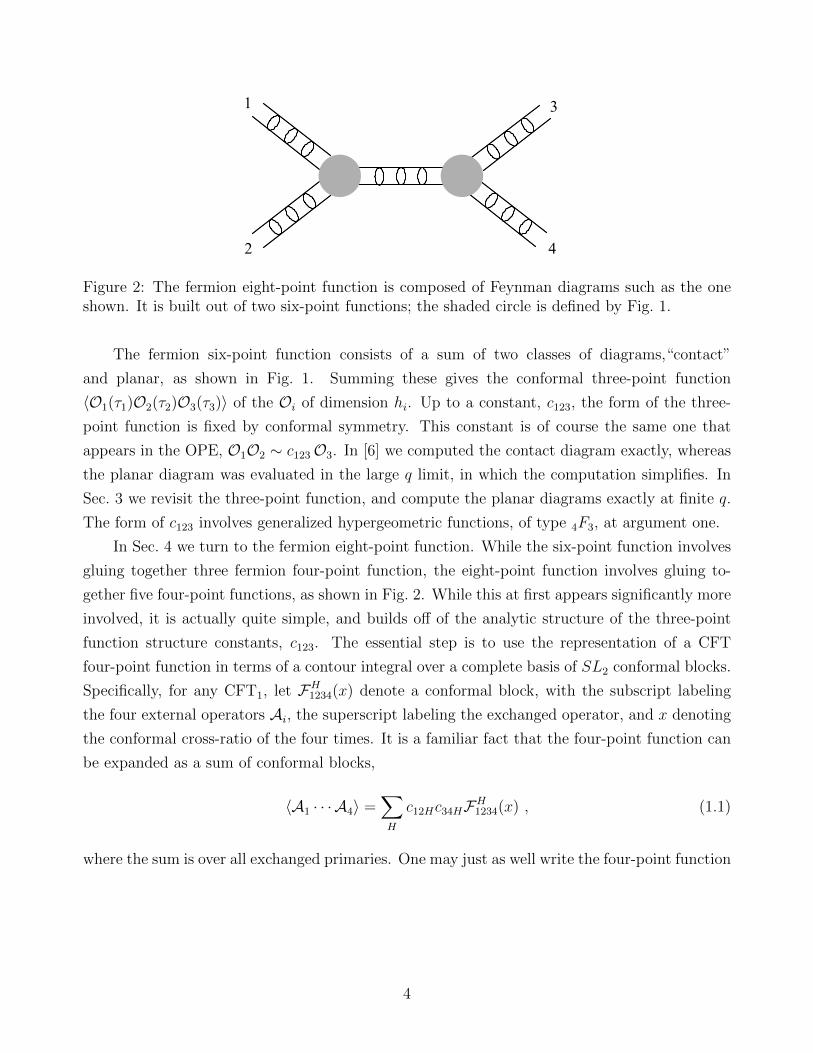
Figure 2: The fermion eight-point function is composed of Feynman diagrams such as the oneshown. It is built out of two six-point functions; the shaded circle is defined by Fig. 1.
The fermion six-point function consists of a sum of two classes of diagrams,“contact”
and planar, as shown in Fig. 1. Summing these gives the conformal three-point function
〈O1(τ1)O2(τ2)O3(τ3)〉 of the Oi of dimension hi. Up to a constant, c123, the form of the three-
point function is fixed by conformal symmetry. This constant is of course the same one that
appears in the OPE, O1O2 ∼ c123O3. In [6] we computed the contact diagram exactly, whereas
the planar diagram was evaluated in the large q limit, in which the computation simplifies. In
Sec. 3 we revisit the three-point function, and compute the planar diagrams exactly at finite q.
The form of c123 involves generalized hypergeometric functions, of type 4F3, at argument one.
In Sec. 4 we turn to the fermion eight-point function. While the six-point function involves
gluing together three fermion four-point function, the eight-point function involves gluing to-
gether five four-point functions, as shown in Fig. 2. While this at first appears significantly more
involved, it is actually quite simple, and builds off of the analytic structure of the three-point
function structure constants, c123. The essential step is to use the representation of a CFT
four-point function in terms of a contour integral over a complete basis of SL2 conformal blocks.
Specifically, for any CFT1, let FH1234(x) denote a conformal block, with the subscript labeling
the four external operators Ai, the superscript labeling the exchanged operator, and x denoting
the conformal cross-ratio of the four times. It is a familiar fact that the four-point function can
be expanded as a sum of conformal blocks,
〈A1 · · · A4〉 =∑H
c12Hc34HFH1234(x) , (1.1)
where the sum is over all exchanged primaries. One may just as well write the four-point function
4

as a contour integral, 1
〈A1 · · · A4〉 =
∫C
dh
2πif(h)Fh1234(x) , (1.2)
with some appropriately chosen f(h), where the contour consists of a line running parallel to
the imaginary axis, h = 12
+ is, as well as circles around the positive even integers, h = 2n.
The distinction between these two expansions is that the former sums over conformal blocks
corresponding to physical operators in the theory, whereas the latter sums over the blocks that
form a complete basis. If one closes the contour in the latter, one recovers the sum in the former.
Let us write the SYK fermion four-point function in the form of such a contour integral,
∑ij
〈χi(τ1)χi(τ2)χj(τ3)χj(τ4)〉 =
∫C
dh
2πiρ(h)Fh∆(x) . (1.3)
Closing the contour yields the standard conformal block expansion, with OPE coefficients∑i χiχi ∼
∑hnchnOhn , given by,
c2hn
= −Res ρ(h)∣∣∣h=hn
. (1.4)
The main step in evaluating the contribution to the SYK four-point function 〈O1 · · · O4〉 shown in
Fig. 2, is to use the above contour integral representation for the intermediate fermion four-point
function. After some manipulation, we will find these diagrams are,
〈O1(τ1) · · · O4(τ4)〉s =
∫C
dh
2πi
ρ(h)
c2h
c12hc34hFh1234(x) . (1.5)
This result is simple and intuitive, following Feynman-like rules: there are cubic interactions
c12h and c34h, the conformal block of Oh, Fh1234, acts as the CFT analog of a propagator, and
h-space acts as the CFT analog of Fourier space.
If one closes the contour in (1.5), one is left with the standard representation of a CFT
four-point function as a sum of conformal blocks. The analytic structure of the integrand is
such that the only blocks that appear are those corresponding to single-trace and double-trace
operators, as should be the case. In fact, the argument leading to (1.5) is general, and is valid
for any cubic level interactions of four-point functions, not necessarily the ones specific to SYK
that were depicted in Fig. 1.
The expression (1.5) is just for the s-channel diagrams. We must also include the t-channel
and u-channel diagrams, which follow from the s-channel ones by a simple permutation of
1 We are being slightly imprecise here, in that what should really enter this expression is the conformal blockplus its shadow; we will be more explicit in the main body of the paper.
5
operators. In adding these three contributions, we will over-count the diagram which has no
exchanged melons, shown later in Fig. 12, which must then be explicitly subtracted off.
Outline
The paper is organized as follows: Sec. 2 reviews the SYK model and the fermion four-point
function. The bilinear three-point function is computed in Sec. 3 and the bilinear four-point
function is computed in Sec. 4. Higher-point functions are studied in Sec. 5. The correlation
functions of the bilinears, in the limit that all of them have large dimension, reduce to the
correlators of generalized free field theory of fermions in the singlet sector. This provides a
good way of studying their asymptotic behavior, via saddle point, and is discussed in Sec. 6. In
Sec. 7, we make some comments on what the correlators teach us about the bulk dual of SYK,
and discuss the relation between exchange Feynman diagrams in SYK and exchange Witten
diagrams. We end in Sec. 8 with a brief discussion.
In Appendix. A we review conformal blocks, the shadow formalism, and Mellin space. Ap-
pendix. B discusses the SYK correlation functions in the large q limit, and Appendix. C discusses
the generalized free field limit. In Appendix. D we discuss the relation between the fermion cor-
relation functions and the bilinear correlation functions. In Appendix. E we study additional
contact Feynman diagrams that must be included in the computation of correlation functions
if q is sufficiently large. In Appendix. F we express exchange and contact Witten diagrams
as sums of conformal blocks. In Appendix. G we show that the spectrum of large q SYK can
be reproduced by placing an AdS2 brane inside of AdS3, however this does not reproduce the
necessary cubic couplings.
2. SYK Ladders
2.1. SYK basics
The SYK model describes N � 1 Majorana fermions satisfying {χi, χj} = δij, with action,
Stop + SintSY K , where,
Stop =1
2
N∑i=1
∫dτ χi
d
dτχi , (2.1)
is the action for free Majorana fermions, and the interaction is,
SintSY K =
(i)q2
q!
N∑i1,...,iq=1
∫dτ Ji1 i2 ...iq χi1χi2 · · ·χiq , (2.2)
6

where the coupling Ji1,...,iq is totally antisymmetric and, for each i1, . . . , iq, is chosen from a
Gaussian ensemble, with variance,
1
(q − 1)!
N∑i2,...,iq=1
〈Ji1i2...iqJi1i2...iq〉 = J2 . (2.3)
One can consider SYK for any even q ≥ 2, with q = 4 being the prototypical case.
In the UV, at zero coupling, the total action is (2.1), and the fermions have a two-point
function given by 12sgn(τ). In the infrared, for J |τ | � 1, the fermion two-point function is, at
leading order in 1/N ,
G(τ) = bsgn(τ)
|Jτ |2∆, (2.4)
where b is given by,
ψ(∆) ≡ 2i√π 2−2∆ Γ(1−∆)
Γ(12
+ ∆), bq = − 1
ψ(∆)ψ(1−∆)=
1
2π(1− 2∆) tanπ∆ , (2.5)
and the IR dimension of the fermions is ∆ = 1/q.
While SYK appears conformally invariant at the level of the two-point function, the confor-
mal invariance is broken at the level of the four-point function [5, 7, 8], resulting in SYK being
“nearly” conformally invariant in the infrared. There is a variant of SYK, cSYK [9], which is
conformally invariant at strong coupling, and in fact, for any value of the coupling. The action
for cSYK is S0 + SintSY K , where Sint
SY K is given by (2.2), while S0 is the bilocal action,
S0 = bqN∑i=1
∫dτ1dτ2 χi(τ1)
sgn(τ1 − τ2)
|τ1 − τ2|2(1−∆)χi(τ2) . (2.6)
The distinction between SYK and cSYK is in the kinetic term, Stop versus S0. As a result, for
SYK the coupling J is dimension-one, while for cSYK it is dimensionless.
At strong coupling, the correlation functions of all bilinear, primary, O(N) singlet operators
On, schematically of the form On =∑N
i=1 χi∂1+2nτ χi, are the same for SYK and for cSYK, for
n ≥ 1. The distinction between SYK and cSYK appears in the correlators involving O0 (the
“h = 2” operator); it is these that break conformal invariance in SYK. Our results for the
correlation functions of the On that will be presented in the body of the paper are for cSYK at
strong coupling, or, equivalently, for all the On in SYK at strong coupling, with the exception
of those correlators involving O0. 2 Since cSYK is conformally invariant for all J , it is trivial to
2In particular, the fermion four-point function in SYK, has a block coming from O0 that breaks conformalinvariance and, at finite temperature, scales as βJ . We will not be including this contribution. It would give rise
7

+ + . . .+
Figure 3: The fermion four-point function, at order 1/N , is a sum of ladder diagrams. Thereare also crossed diagrams, which are not shown.
extend the results to cSYK correlators at finite J .
2.2. Fermion four-point function: summing ladders
The SYK four-point function to order 1/N , is given by,
1
N2
N∑i,j=1
〈χi(τ1)χi(τ2)χj(τ3)χj(τ4)〉 = G(τ12)G(τ34) +1
NF(τ1, τ2, τ3, τ4) , (2.7)
where τ12 ≡ τ1 − τ2 and F is given by the sum of ladder diagrams, as shown in Fig. 3. Due to
the restored O(N) invariance the leading behavior in 1/N is completely captured by F . The
first diagram in Fig. 3, although disconnected, is suppressed by 1/N as it requires setting the
indices to be equal, i = j. This diagram is denoted by F0,
F0 = −G(τ13)G(τ24) +G(τ14)G(τ23) . (2.8)
Letting K denote the kernel that adds a rung to the ladder,
K(τ1, . . . τ4) = −(q − 1)J2G(τ13)G(τ24)G(τ34)q−2 , (2.9)
and then summing the ladders yields, schematically, F = (1 +K +K2 + . . .)F0 = (1−K)−1F0.
To write this explicitly, one should decompose F0 in terms of a complete basis of eigenvectors
of the kernel K.
The eigenvectors of the kernel are conformal three-point functions involving two fermions
and a scalar of dimension h, 3
〈Oh(τ0)χ(τ1)χ(τ2)〉 = chb
J2∆
sgn(τ12)
|τ12|2∆−h|τ01|h|τ02|h, (2.10)
to terms in the higher-point functions that scale as powers of βJ , and are straightforward to compute, using theO0 block in the fermion four-point function.
3In the current context the subscript on Oh denotes that the operator has dimension h. This is differentfrom another usage of subscript, On, which denotes the operator in SYK, which in the weak coupling limit hasdimension 2∆ + 2n+ 1. Finally, we will also sometimes use the shorthand O1 to mean Oh1
.
8

2 4 6 8
Figure 4: The contour of integration C in the complex h-plane.
and have corresponding eigenvalues [5],
kc(h) = −(q − 1)ψ(∆)
ψ(1−∆)
ψ(1−∆− h2)
ψ(∆− h2)
, (2.11)
where ψ(∆) was defined in (2.5). For our purposes, one should regard the right side of (2.10)
as defining what we mean by the left side. It is manifest that kc(h) = kc(1− h), and moreover,
that the singularities of kc(h) in the right-half complex plane are at h = 2∆ + 2n+ 1, for integer
n. The three-point function involving the shadow of Oh, 〈O1−hχχ〉 is also an eigenfunction of
the kernel, with the same eigenvalue, kc(h). As a result, Ψh, defined as [8],
2 chc1−hb sgn(τ12) b sgn(τ34)
|Jτ12|2∆|Jτ34|2∆Ψh(x) =
∫dτ0 〈χ(τ1)χ(τ2)Oh(τ0)〉〈χ(τ3)χ(τ4)O1−h(τ0)〉 , (2.12)
is also an eigenfunction of the kernel. Moreover, (2.12) can be seen to be an eigenfunction of the
SL(2, R) Casimir, and is simply the sum of a conformal block and its shadow, see Appendix A.
The conformal cross-ratio of times, x, is defined as,
x =τ12τ34
τ13τ24
. (2.13)
The necessary range of h in order to form a complete basis is dictated by representation
theory of the conformal group. In even spacetime dimensions, one only needs the continuous
series, h = d2
+ is, where d is the dimension and −∞ < s <∞. In odd dimensions, the case
relevant for SYK, one must also include the discrete series, h = 2n for n ≥ 1. The eigenfunctions
are orthonormal with respect to the Plancherel measure,
µ(h) =2h− 1
π tan πh2
. (2.14)
The measure has poles at h = 2n; indeed, the complete basis includes the discrete series specif-
9
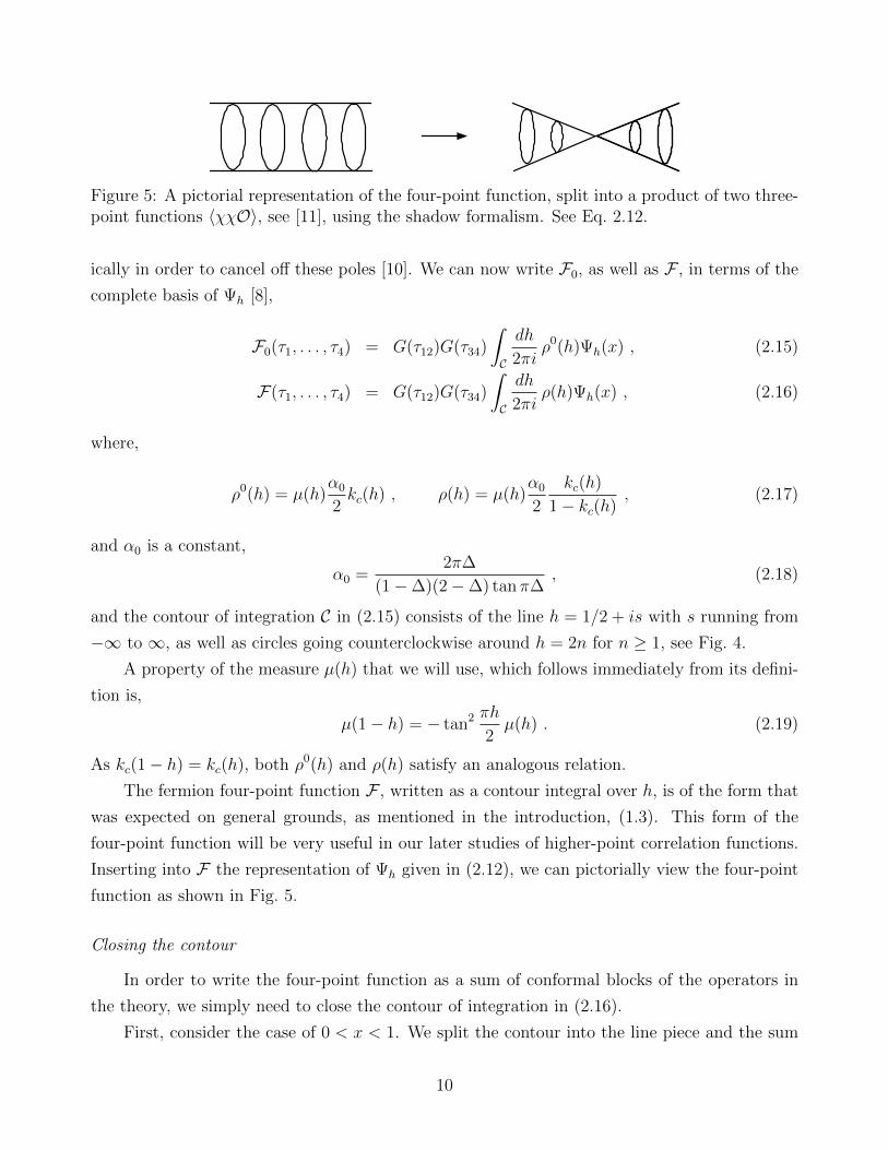
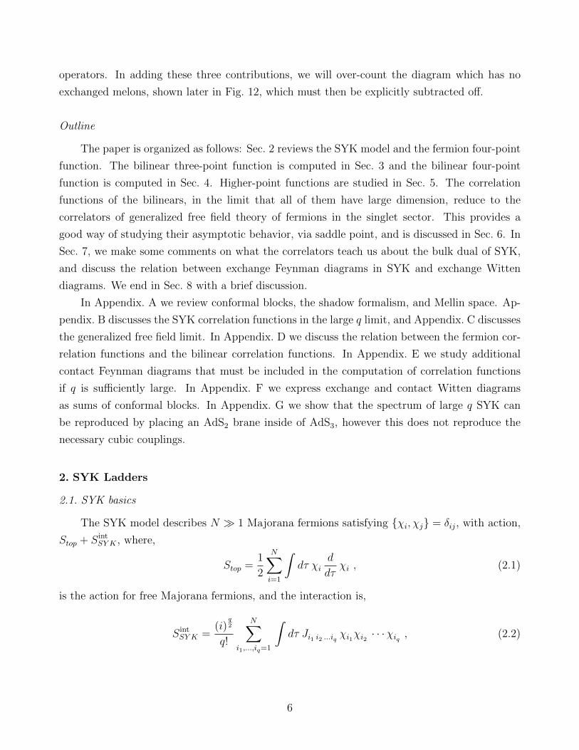
Figure 5: A pictorial representation of the four-point function, split into a product of two three-point functions 〈χχO〉, see [11], using the shadow formalism. See Eq. 2.12.
ically in order to cancel off these poles [10]. We can now write F0, as well as F , in terms of the
complete basis of Ψh [8],
F0(τ1, . . . , τ4) = G(τ12)G(τ34)
∫C
dh
2πiρ0(h)Ψh(x) , (2.15)
F(τ1, . . . , τ4) = G(τ12)G(τ34)
∫C
dh
2πiρ(h)Ψh(x) , (2.16)
where,
ρ0(h) = µ(h)α0
2kc(h) , ρ(h) = µ(h)
α0
2
kc(h)
1− kc(h), (2.17)
and α0 is a constant,
α0 =2π∆
(1−∆)(2−∆) tanπ∆, (2.18)
and the contour of integration C in (2.15) consists of the line h = 1/2 + is with s running from
−∞ to ∞, as well as circles going counterclockwise around h = 2n for n ≥ 1, see Fig. 4.
A property of the measure µ(h) that we will use, which follows immediately from its defini-
tion is,
µ(1− h) = − tan2 πh
2µ(h) . (2.19)
As kc(1− h) = kc(h), both ρ0(h) and ρ(h) satisfy an analogous relation.
The fermion four-point function F , written as a contour integral over h, is of the form that
was expected on general grounds, as mentioned in the introduction, (1.3). This form of the
four-point function will be very useful in our later studies of higher-point correlation functions.
Inserting into F the representation of Ψh given in (2.12), we can pictorially view the four-point
function as shown in Fig. 5.
Closing the contour
In order to write the four-point function as a sum of conformal blocks of the operators in
the theory, we simply need to close the contour of integration in (2.16).
First, consider the case of 0 < x < 1. We split the contour into the line piece and the sum
10

of poles, ∫C
dh
2πiρ(h)Ψh(x) =
∫h= 1
2+is
dh
2πiρ(h)Ψh(x) +
∑n>0
Res ρ(h) Ψh(x)∣∣∣h=2n
. (2.20)
Focusing first on the line piece of the contour, we write Ψh in terms of a sum of a conformal
block and its shadow, see Appendix. A,
G(τ12)G(τ34)
∫12
+is
dh
2πiρ(h)Ψh(x) =
b2
2J4∆
∫12
+is
dh
2πiρ(h)
[β(h, 0)Fh∆(x) + β(1−h, 0)F1−h
∆ (x)],
(2.21)
where Fh∆ is the conformal block with external fermions of dimension ∆ and an exchanged scalar
of dimension h, while,
β(h, 0) =√π
Γ(h2)2Γ(1
2− h)
Γ(1−h2
)2Γ(h). (2.22)
In (2.21), let us change integration variables for the second term, h→ 1− h, use the reflection
relation (2.19) for the measure, as well as,
β(h, 0)
(1− tan2 πh
2
)= 2
Γ(h)2
Γ(2h), (2.23)
to write,
G(τ12)G(τ34)
∫12
+is
dh
2πiρ(h)Ψh(x) =
b2
J4∆
∫12
+is
dh
2πiρ(h)
Γ(h)2
Γ(2h)Fh∆(x) . (2.24)
Turning now to the sum over the discrete series, we rewrite this as,
G(τ12)G(τ34)∑n>0
Res ρ(h) Ψh(x)∣∣∣h=2n
=b2
J4∆
∑n>0
Res ρ(h)Γ(h)2
Γ(2h)Fh∆(x)
∣∣∣h=2n
, (2.25)
where we have used that β(1 − 2n, 0) = 0 for n > 0 and β(h, 0) = 2Γ(h)2/Γ(2h) for h = 2n.
Recombining the continuous and discrete series terms gives,
F(τ1, . . . , τ4) =b2
J4∆
∫C
dh
2πiρ(h)
Γ(h)2
Γ(2h)Fh∆(x) . (2.26)
Finally, we close the line piece of the contour to the right, giving a sum over the poles at the h
11

for which kc(h) = 1, 4
F(τ1, . . . , τ4) =b2
J4∆
∑hn
c2nF
hn∆ (x) , 0 < x < 1 , (2.27)
where hn are the single-trace operator dimensions, kc(hn) = 1, and we have defined [8] 5
c2n ≡ −Res ρ(h)
∣∣∣h=hn
Γ(hn)2
Γ(2hn)= α0
(hn − 1/2)
π tan(πhn/2)
Γ(hn)2
Γ(2hn)
1
k′c(hn). (2.28)
One can identify the cn as the OPE coefficients 1N
∑Ni=1 χ(0)χ(τ) ∼ 1√
N
∑n cnOn. We will
sometimes use the short-hand, ch1(or c1) to denote cn for h1 that is given by h1 = 2∆ + 2n+ 1
at weak coupling.
This is the expression for the fermion four-point function when the conformal cross-ratio x
in the range 0 < x < 1. For the case of x > 1, we return to (2.16) and simply close the line piece
of the contour to the right, giving,
F(τ1, . . . , τ4) = G(τ12)G(τ34)∑hn
Res ρ(h)∣∣∣h=hn
Ψhn(x) , x > 1 . (2.29)
We conclude with a comment on the singularity structure in h-space of the ladder diagrams.
One can see that the first diagram in the sequence of ladders, F0, is, in h-space, proportional
to kc(h). Similarly, a diagram with n rungs is proportional to kc(h)n+1. Summing any finite
number of ladder diagrams gives a polynomial in kc(h) which, like kc(h), will have singularities
at h = 2∆ + 2n + 1. Correspondingly, upon closing the contour to return to physical space,
the finite sum of ladder diagrams will be expressed in terms of conformal blocks of exchanged
operators of dimension 2∆ + 2n + 1: the free-field dimensions of the primaries, schematically
of the form∑χi∂
2n+1τ χi. It is only when one sums an infinite number of ladder diagrams,
such as the geometric sum kc(h)(1 + kc(h) + kc(h)2 + . . .), as in ρ(h) appearing in F , that the
singularities of the expression are no longer where kc(h) is singular, but rather where kc(h) = 1.
Correspondingly, the expansion of F is in terms of conformal blocks at the infrared dimensions
of the primaries, the h for which kc(h) = 1.
4The poles at h = 2n coming from measure µ(h) are outside of the closed contour, as a result of the piece ofthe contour made up of the circles at h = 2n.
5We have suppressed the 1/N scaling of cn ∼ 1/√N . In order to not carry around factors of 1/N , we will
generally suppress them. A connected p-point correlation function scales as 〈O1 · · · Op〉 ∼ 1/N(p−2)
2 .
12
+ + + + . . .
Figure 6: The first set of diagrams (“contact” diagrams) contributing to the six-point functionat order 1/N2.
3. Bilinear Three-Point Function
In this section we compute, to leading nontrivial order in 1/N , the fermion six-point function,
and correspondingly the three-point function 〈O1O2O3〉 of the bilinear O(N) invariant primaries,
Oi, of dimension hi.
The six-point function of the fermions can be written as,
1
N3
N∑i,j,l=1
〈χi(τ1)χi(τ2)χj(τ3)χj(τ4)χl(τ5)χl(τ6)〉 = . . .+1
N2S(τ1, . . . , τ6) + . . . , (3.1)
where S is the lowest order term in 1/N that contains fully connected diagrams. There are two
classes of diagrams contributing to S: the “contact” diagrams, whose sum we denote by S1, and
the planar diagrams, whose sum we denote by S2,
S = S1 + S2 . (3.2)
We study the contact diagrams in Sec. 3.1, and the planar diagrams in Sec. 3.2.
From the fermion six-point function, we will extract the three-point function of the bilinear
primary O(N) singlets,
〈O1(τ1)O2(τ2)O3(τ3)〉 =1√N
c123
|τ12|h1+h2−h3 |τ23|h2+h3−h1 |τ13|h1+h3−h2, (3.3)
where c123 will have two contributions,
c123 = c(1)123 + c
(2)123 , (3.4)
coming from the contact and the planar diagrams, respectively. We compute c(1)123 in Sec. 3.1 and
c(2)123 in Sec. 3.2.
13

3.1. Contact diagrams
The “contact diagrams” are composed of three fermion four-point functions glued to two
interaction vertices connected by q−3 propagators, see Fig. 6 and the first diagram on the right
in Fig. 1,
S1 = (q − 1)(q − 2)J2
∫dτadτbG(τab)
q−3F(τ1, τ2, τa, τb)F(τ3, τ4, τa, τb)F(τ5, τ6, τa, τb) . (3.5)
The fermion four-point function F is a sum of conformal blocks, and the functional form of each
block is fixed by conformal invariance. It will be most convenient to write the blocks in terms of
the differential operator Cn(τ12, ∂2), which sums the contributions of all descendants associated
with the primary On, acting on a conformal three-point function, see Appendix A,
F(τ1, τ2, τa, τb) =∑n
cn Cn(τ12, ∂2) 〈On(τ2)χ(τa)χ(τb)〉 , (3.6)
where the three-point function was given in (2.10). Using this form for each of the four-point
functions appearing in S1 gives,
S1 =∑
n1,n2,n3
3∏i=1
cniCni(τ2i−1,2i, ∂2i) 〈On1(τ2)On2
(τ4)On3(τ6)〉1 , (3.7)
where,
〈On1(τ1)On2
(τ2)On3(τ3)〉1 = (q − 1)(q − 2)J2
∫dτadτbG(τab)
q−33∏i=1
〈Oni(τi)χ(τa)χ(τb)〉 . (3.8)
Explicitly writing out the integrand in the expression for the three-point function of bilinears
gives,
〈On1(τ1)On2
(τ2)On3(τ3)〉1 = cn1
cn2cn3
(q − 1)(q − 2)bq I(1)123(τ1, τ2, τ3) , (3.9)
where
I(1)123(τ1, τ2, τ3) =
∫dτadτb
|τab|h1+h2+h3−2
|τ1a|h1 |τ1b|h1|τ2a|h2|τ2b|h2|τ3a|h3|τ3b|h3. (3.10)
In order to evaluate the integral, it is convenient to change integration variables to the two
cross-ratios,
A =τa1τ23
τa2τ13
, B =τb2τ13
τb1τ23
, (3.11)
14
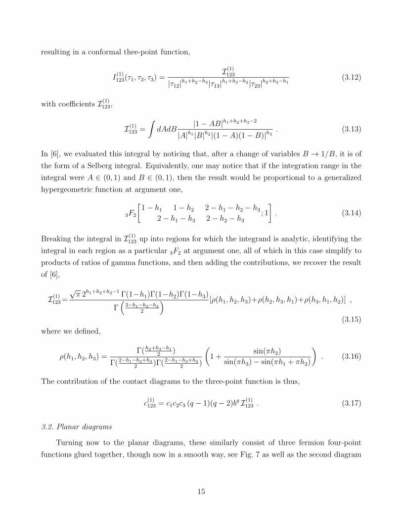
resulting in a conformal thee-point function,
I(1)123(τ1, τ2, τ3) =
I(1)123
|τ12|h1+h2−h3|τ13|h1+h3−h2|τ23|h2+h3−h1(3.12)
with coefficients I(1)123,
I(1)123 =
∫dAdB
|1− AB|h1+h2+h3−2
|A|h1|B|h2|(1− A)(1−B)|h3. (3.13)
In [6], we evaluated this integral by noticing that, after a change of variables B → 1/B, it is of
the form of a Selberg integral. Equivalently, one may notice that if the integration range in the
integral were A ∈ (0, 1) and B ∈ (0, 1), then the result would be proportional to a generalized
hypergeometric function at argument one,
3F2
[1− h1 1− h2 2− h1 − h2 − h3
2− h1 − h3 2− h2 − h3
; 1
]. (3.14)
Breaking the integral in I(1)123 up into regions for which the integrand is analytic, identifying the
integral in each region as a particular 3F2 at argument one, all of which in this case simplify to
products of ratios of gamma functions, and then adding the contributions, we recover the result
of [6],
I(1)123 =
√π 2h1+h2+h3−1 Γ(1−h1)Γ(1−h2)Γ(1−h3)
Γ(
3−h1−h2−h2
2
) [ρ(h1, h2, h3)+ρ(h2, h3, h1)+ρ(h3, h1, h2)] ,
(3.15)
where we defined,
ρ(h1, h2, h3) =Γ(h2+h3−h1
2)
Γ(2−h1−h2+h3
2)Γ(2−h1−h3+h2
2)
(1 +
sin(πh2)
sin(πh3)− sin(πh1 + πh2)
). (3.16)
The contribution of the contact diagrams to the three-point function is thus,
c(1)123 = c1c2c3 (q − 1)(q − 2)bq I(1)
123 . (3.17)
3.2. Planar diagrams
Turning now to the planar diagrams, these similarly consist of three fermion four-point
functions glued together, though now in a smooth way, see Fig. 7 as well as the second diagram
15
+ + + + . . .
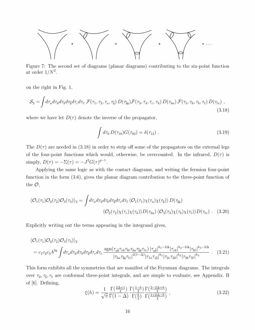
Figure 7: The second set of diagrams (planar diagrams) contributing to the six-point functionat order 1/N2.
on the right in Fig. 1,
S2 =
∫dτadτadτbdτbdτcdτc F(τ1, τ2, τa, τb)D(τbb)F(τ3, τ4, τc, τa)D(τaa)F(τ5, τ6, τb, τc)D(τcc) ,
(3.18)
where we have let D(τ) denote the inverse of the propagator,∫dτ0D(τ10)G(τ02) = δ(τ12) . (3.19)
The D(τ) are needed in (3.18) in order to strip off some of the propagators on the external legs
of the four-point functions which would, otherwise, be overcounted. In the infrared, D(τ) is
simply, D(τ) = −Σ(τ) = −J2G(τ)q−1.
Applying the same logic as with the contact diagrams, and writing the fermion four-point
function in the form (3.6), gives the planar diagram contribution to the three-point function of
the O,
〈O1(τ1)O2(τ2)O3(τ3)〉2 =
∫dτadτadτbdτbdτcdτc 〈O1(τ1)χ(τa)χ(τb)〉D(τbb)
〈O2(τ2)χ(τc)χ(τa)〉D(τaa) 〈O3(τ3)χ(τb)χ(τc)〉D(τcc) . (3.20)
Explicitly writing out the terms appearing in the integrand gives,
〈O1(τ1)O2(τ2)O3(τ3)〉2
= c1c2c3 b3q
∫dτadτadτbdτbdτcdτc
sgn(τabτcaτbcτaaτbbτcc) |τab|h1−2∆|τca|h2−2∆|τbc|h3−2∆
|τaaτbbτcc|2(1−∆)|τ1aτ1b|
h1|τ2cτ2a|h2|τ3bτ3c|h3. (3.21)
This form exhibits all the symmetries that are manifest of the Feynman diagrams. The integrals
over τa, τb, τc are conformal three-point integrals, and are simple to evaluate, see Appendix. B
of [6]. Defining,
ξ(h) =1√π
Γ(2∆+12
)
Γ(1−∆)
Γ(1−h2
)
Γ(h2)
Γ(2−2∆+h2
)
Γ(1+2∆−h2
), (3.22)
16

gives
〈O1(τ1)O2(τ2)O3(τ3)〉2 = c1c2c3 ξ(h1)ξ(h2)ξ(h3) I(2)123(τ1, τ2, τ3) , (3.23)
where [6],
I(2)123(τ1,τ2,τ3)=
∫dτadτbdτc
−sgn(τ1aτ1bτ2aτ2cτ3bτ3c)|τab|h1−1|τca|h2−1|τbc|h3−1
|τ1a|h1−1+2∆|τ1b|h1+1−2∆|τ2c|h2−1+2∆|τ2a|h2+1−2∆|τ3b|h3−1+2∆|τ3c|h3+1−2∆.
(3.24)
In making the choice of, for instance, evaluating the τa integral instead of the τa integral, some
of the symmetries are no longer manifest.
To proceed with evaluating the remaining three integral, we change integration variables to
the cross-ratios A,B,C, defined as,
A =τa1τ32
τa2τ31
, B =τ13τabτ1aτ3b
, C =τ2aτ3c
τ23τac. (3.25)
This change of variables transforms I(2)123 into a form that is manifestly a conformal three-point
function,
I(2)123(τ1, τ2, τ3) =
I(2)123
|τ12|h1+h2−h3 |τ13|h1+h3−h2 |τ23|h2+h3−h1, (3.26)
with a coefficient,
I(2)123 =
∫dAdBdC
sgn(C(1−B)(1− C)) |1− ABC|h3−1
|A|h1 |1− A|1−h1−h2+h3|B|1−h1|1−B|h1+1−2∆|C|1−2∆+h3|1− C|h2−1+2∆.
(3.27)
To evaluate this integral we note the following: if the integration range were over A ∈(0, 1), B ∈ (0, 1), C ∈ (0, 1), then this would be of the form of a generalized hypergeometric
function at argument equal to one,
4F3
[1−h1 h1 2∆−h3 1−h3
1+h2−h3 2∆ 2−h2−h3
; 1
]. (3.28)
In order to account for the other regions of integration, one should consider each region separately
and perform simple changes of variables combined with 2F1 connection identities and Euler’s
integral transform,
pFq
[a1 . . . apb1 . . . bq
; z
]=
Γ(bq)
Γ(ap)Γ(bq − ap)
∫ 1
0
dt tap−1(1− t)bq−ap−1p−1Fq−1
[a1 . . . ap−1
b1 . . . bq−1
; tz
].
A faster method is the following. Consider the more general integral, which is a function of
17

an additional variable z,
I(2)123(z) =
∫dAdBdC
sgn(C(1−B)(1− C)) |1− zABC|h3−1
|A|h1|1− A|1−h1−h2+h3|B|1−h1 |1−B|h1+1−2∆|C|1−2∆+h3|1− C|h2−1+2∆.
(3.29)
The generalized hypergeometric function 4F3 satisfies a fourth-order differential equation. Since
the piece of this integral coming from the region A ∈ (0, 1), B ∈ (0, 1), C ∈ (0, 1) is a 4F3, of the
type (3.28), it must be the case that the integrand satisfies the appropriate differential equation.
Breaking the integral up into regions in which the integrand is analytic, the integrand in each
region should also satisfy the same differential equation. As there are four solutions to the
differential equation defining 4F3, the integral (3.29) should take a form that is a superposition
of these, with some coefficients, αi,6
I(2)123(z) = α1 4F3
[1−h1 h1 2∆−h3 1−h3
1+h2−h3 2∆ 2−h2−h3
; z
]
+ α2 zh3−h2
4F3
[1−h1−h2+h3 h1−h2+h3 2∆−h2 1−h2
2−2h2 1−h2+h3 2∆−h2+h3
; z
]
+ α3 z1−2∆
4F3
[2−h1−2∆ 1+h1−2∆ 1−h3 2−h3−2∆
2+h2−h3−2∆ 3−h2−h3−2∆ 2−2∆; z
]
+ α4 zh2+h3−1
4F3
[h2+h3−h1 h1+h2+h3−1 h2−1+2∆ h2
2h2 h2+h3−1+2∆ h2+h3
; z
]. (3.30)
To fix the coefficient α1 we simply set z = 0 in (3.29): the integrals decouple, and are trivial to
evaluate, see Appendix. B of [6] for relevant equations. Similarly to fix α2, we change integration
variables A→ A/(zBC), and then take small z and evaluate the integral. To fix α3 we change
variables B → B/(zAC), and for α4 we change variables C → C/(zAB). It is convenient to
define αi, which is related to αi through the coefficients ξ(h) that arose earlier in performing the
first three of six integrals,
αi = ξ(h1)ξ(h2)ξ(h3)αi . (3.31)
6It is conceivable that, as result of boundary terms, this is not true. However, we have also evaluated theintegral (3.27) explicitly, by breaking it up into regions, as outlined in the previous paragraph, and found thesame answer as the one quoted below, though in a less nice form.
18
The result for the αi is the following,
α1 = −Γ(2∆+1
2)2
Γ(1−∆)2
3∏i=1
Γ(1−hi2
)
Γ(hi2
)
Γ(3−h2−2∆2
)Γ(2+h2−2∆2
)
Γ(h2+2∆2
)Γ(1−h2+2∆2
)
Γ(h3−h2
2)Γ(h2+h3−1
2)
Γ(2−h2−h3
2)Γ(1+h2−h3
2)
Γ(h1+h2−h3
2)
Γ(1−h1−h2+h3
2),
α2 = −Γ(2∆+1
2)3
Γ(1−∆)3
Γ(1−h1
2)
Γ(h1
2)
Γ(1−h2
2)2 Γ(2h2−1
2)
Γ(h2
2)2 Γ(2−2h2
2)
Γ(3−h2−2∆2
)
Γ(h2+2∆2
)
Γ(2+h3−2∆2
)
Γ(1−h3+2∆2
)
·Γ(h2−h3
2)Γ(h2−h3+2−2∆
2)
Γ(1−h2+h3
2)Γ(h3−h2+1+2∆
2)
Γ(h1−h2+h3
2)
Γ(1−h1+h2−h3
2),
α3 = −Γ(2∆+1
2)3 Γ(∆)
Γ(1−∆)3 Γ(3−2∆2
)
3∏i=1
Γ(1−hi2
)Γ(2+hi−2∆2
)Γ(3−hi−2∆2
)
Γ(hi2
)Γ(1−hi+2∆2
)Γ(hi+2∆2
)
·Γ(h3−h2+2∆
2)Γ(h2+h3−1+2∆
2)
Γ(3+h2−h3−2∆2
)Γ(4−h2−h3−2∆2
)
Γ(h1+h2−h3
2)
Γ(1−h1−h2+h3
2),
α4 = −Γ(2∆+1
2)3
Γ(1−∆)3
Γ(1−h1
2)
Γ(h1
2)
Γ(1−2h2
2)
Γ(h2)
Γ(2+h2−2∆2
)
Γ(1−h2+2∆2
)
Γ(2+h3−2∆2
)
Γ(1−h3+2∆2
)
·Γ(1−h2−h3
2)
Γ(h2+h3
2)
Γ(3−h2−h3−2∆2
)
Γ(h2+h3+2∆2
)
Γ(h1+h2−h3
2)Γ(−h1+h2+h3
2)Γ(h1+h2+h3−1
2)
Γ(1−h1−h2+h3
2)Γ(1+h1−h2−h3
2)Γ(2−h1−h2−h3
2). (3.32)
This completes the evaluation of the planar diagram contribution to the three-point function.
The result is,
c(2)123 = c1c2c3 ξ(h1)ξ(h2)ξ(h3) I(2)
123 , (3.33)
where I(2)123 is a sum of four generalized hypergeometric functions with argument one, I(2)
123 =
I(2)123(z = 1) given by (3.30). Although it is not manifest, c
(2)123 must be symmetric under all
permutations of the hi. In Appendix. B we study c(2)123 in the large q limit in which it somewhat
simplifies.
Universality
The full three-point function coefficient is a sum of the contact diagram and the planar
diagram contributions, c123 = c(1)123 + c
(2)123. It is instructive to write this as,
c123 = c1c2c3I123 . (3.34)
There are two distinct contributions. The product of OPE coefficients ci of two fermions turning
into an Oi reflects the sum of the ladder diagrams; this sum determines the dimensions hi of the
Oi. The contribution I123 comes from gluing the ladders. It is universal in the sense that it is
19
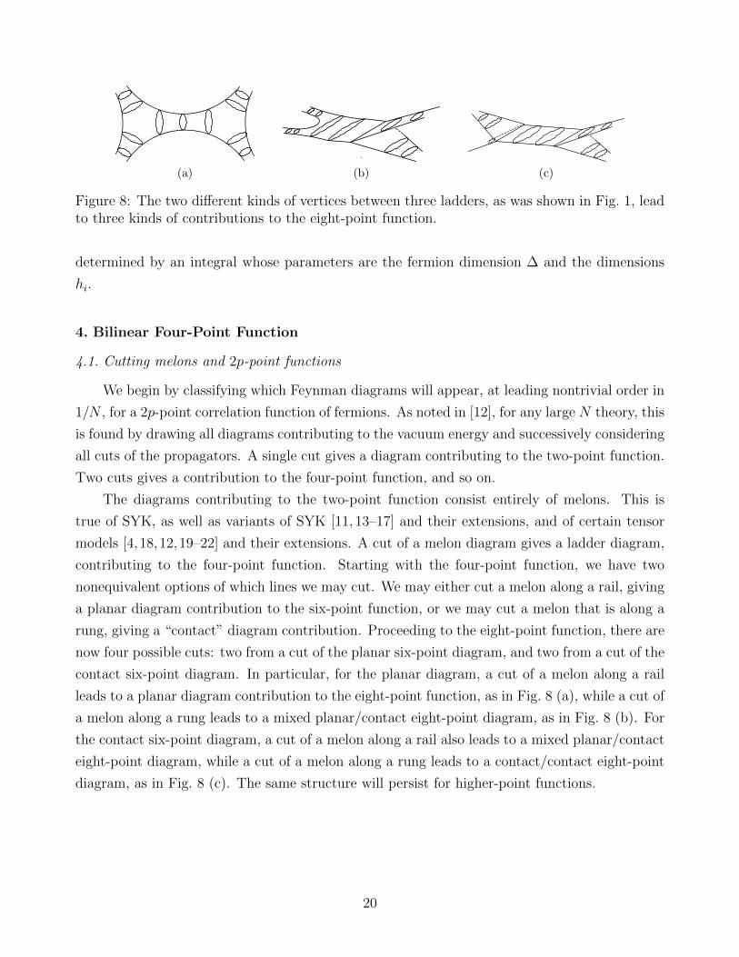
(a) (b) (c)
Figure 8: The two different kinds of vertices between three ladders, as was shown in Fig. 1, leadto three kinds of contributions to the eight-point function.
determined by an integral whose parameters are the fermion dimension ∆ and the dimensions
hi.
4. Bilinear Four-Point Function
4.1. Cutting melons and 2p-point functions
We begin by classifying which Feynman diagrams will appear, at leading nontrivial order in
1/N , for a 2p-point correlation function of fermions. As noted in [12], for any large N theory, this
is found by drawing all diagrams contributing to the vacuum energy and successively considering
all cuts of the propagators. A single cut gives a diagram contributing to the two-point function.
Two cuts gives a contribution to the four-point function, and so on.
The diagrams contributing to the two-point function consist entirely of melons. This is
true of SYK, as well as variants of SYK [11, 13–17] and their extensions, and of certain tensor
models [4,18,12,19–22] and their extensions. A cut of a melon diagram gives a ladder diagram,
contributing to the four-point function. Starting with the four-point function, we have two
nonequivalent options of which lines we may cut. We may either cut a melon along a rail, giving
a planar diagram contribution to the six-point function, or we may cut a melon that is along a
rung, giving a “contact” diagram contribution. Proceeding to the eight-point function, there are
now four possible cuts: two from a cut of the planar six-point diagram, and two from a cut of the
contact six-point diagram. In particular, for the planar diagram, a cut of a melon along a rail
leads to a planar diagram contribution to the eight-point function, as in Fig. 8 (a), while a cut of
a melon along a rung leads to a mixed planar/contact eight-point diagram, as in Fig. 8 (b). For
the contact six-point diagram, a cut of a melon along a rail also leads to a mixed planar/contact
eight-point diagram, while a cut of a melon along a rung leads to a contact/contact eight-point
diagram, as in Fig. 8 (c). The same structure will persist for higher-point functions.
20

+ +
+ + +
1
2 4
3 1 3 1 4
4 2 2 3
1 3 1 3 1 4
2 4 4 2 2 3
Figure 9: Some of the diagrams contributing to the eight-point function. We must includediagrams with melons exchanged in both directions (first and second line).
4.2. Outline
Having established the basic structure of the Feynman diagrams contributing to the eight-
point function, we now list more precisely all the diagrams that will need to summed. Let
Es(τ1, . . . , τ8) denote the Feynman diagram shown previously in Fig. 2, and let 〈O1(τ1) · · · O4(τ4)〉sdenote its contribution to the four-point function of the Oi. In addition, let E0
s (τ1, . . . , τ8), and
correspondingly 〈O1(τ1) · · · O4(τ4)〉0s, denote similar Feynman diagrams, but only the planar
one, and with no exchanged melons, as will be illustrated later in Fig. 12. Then, the four-point
function of the Oi is,
〈O1(τ1) · · · O4(τ4)〉 =(〈O1(τ1) · · · O4(τ4)〉s + (2↔ 3) + (2↔ 4)
)− 1
2
(〈O1(τ1) · · · O4(τ4)〉0s + (2↔ 3) + (2↔ 4)
). (4.1)
Finally, there is an additional diagram, which is discussed in Appendix. E, and consists of four
fermion four-point functions glued to the same melon.
Let us explain why (4.1) is correct. If we, for the moment, focus on only the planar diagrams,
then all the diagrams that need to be summed are shown in Fig. 9. The three classes of diagrams
in the first line are the three different channels. The diagrams in the second line must be included
as well - these are similar to the diagrams on the first line, except now the exchanged melons are
going in the other direction. For the diagrams in which there are no exchanged melons, the top
and bottom diagrams are the same, and we should only include one of them. One can see that
Es(τ1, . . . , τ8) corresponds to the sum of the first and third diagrams on the top line of Fig. 9.
21

Figure 10: The three-point function of bilinears. This looks like the fermion six-point function,with fermions brought together in pairs.
The reason it corresponds to two sets of diagrams is because the fermion four-point function
is antisymmetric under interchange of the last two (or the first two) fermions: in summing the
ladder diagrams, there were two sets of diagrams, coming from adding rungs to the two terms
in F0 in (2.8). The sum of the three terms on the first line of (4.1) accounts for all six terms in
Fig. 9. The second line of (4.1) compensates for the double counting of diagrams in which no
melons are exchanged. Finally, in addition to the diagrams shown in Fig. 9, there are diagrams
in which the cubic vertex is contact rather than planar, such as those in Fig. 8; these have
already been taken into account in (4.1), as the shaded circle in the diagram in Fig. 2 includes
both such vertices, see Fig. 1.
We now turn to computing 〈O1(τ1) · · · O4(τ4)〉s.
4.3. Splitting and recombining conformal blocks
The eight-point function of the fermions can be written as,
1
N4
∑i1,...,i4
〈χi1(τ1)χi1(τ2)χi2(τ3)χi2(τ4)χi3(τ5)χi3(τ6)χi4(τ7)χi4(τ8)〉 = . . .+1
N3E(τ1, . . . , τ8) + . . . ,
(4.2)
where E is the lowest order term in 1/N that contains fully connected diagrams.
In this section we will study the contribution to the eight-point function that was shown
in Fig. 2, denoted by Es(τ1, . . . , τ8). This consists of two six-point functions glued together. We
can write a general expression for the six-point function, containing a piece Score which encodes
the details of the interactions, attached to three external four-point functions,
S(τ1, . . . , τ6)=
∫dτa1· · · dτa6
F(τ1, τ2, τa1, τa2
)F(τ3, τ4, τa3, τa4
)F(τ5, τ6, τa5, τa6
)Score(τa1, . . . , τa6
) .
(4.3)
Pictorially, Score is the shaded circle that appeared before in Fig. 2. For SYK, Score is pictorially
22

Figure 11: An important step in computing the bilinear four-point function is to use the splitrepresentation for the intermediate four-point function, as was shown previously in Fig. 5.
defined in Fig. 1. More explicitly, we found in Sec. 3 that Score is,
Score = (q − 1)(q − 2)J2G(τa1a2)q−3δ(τa1a3
)δ(τa1a5)δ(τa2a4
)δ(τa2a6) +D(τa2a5
)D(τa4a1)D(τa6a3
) ,
however the explicit form of Score is not relevant for the argument that follows.
Employing the same logic as used perviously in the derivation of the three-point function
of bilinears from the six-point function of fermions, and utilizing the conformal block structure
of F given in (3.6), we may write for the three-point function, see Fig. 10,
〈O1(τ1)O2(τ2)O3(τ3)〉 =
∫dτa1· · · dτa6
Score(τa1, . . . , τa6
)
〈O1(τ1)χ(τa1)χ(τa2
)〉〈O2(τ2)χ(τa3)χ(τa4
)〉〈O3(τ3)χ(τa5)χ(τa6
)〉 . (4.4)
With this building block, we construct Es. As shown in Fig. 2, gluing together two six-point
functions gives,
Es(τ1, . . . , τ8) =
∫dτa1· · · dτa8
dτb1 · · · dτb4Score(τa1
, . . . , τa4, τb1 , τb2)Score(τa5
, . . . , τa8, τb3 , τb4)
F(τ1, τ2, τa1, τa2
)F(τ3, τ4, τa3, τa4
)F(τb1 , . . . , τb4)F(τ5, τ6, τa5, τa6
)F(τ7, τ8, τa7, τa8
)
Again using (3.6), the four-point function of the O is thus,
〈O1(τ1) · · · O4(τ4)〉s =
∫dτa1· · · dτa8
dτb1 · · · dτb4Score(τa1
, . . . , τa4, τb1 , τb2)Score(τa5
, . . . , τa8, τb3 , τb4)
〈O1(τ1)χ(τa1)χ(τa2
)〉〈O2(τ2)χ(τa3)χ(τa4
)〉F(τb1 , . . . , τb4)〈O3(τ3)χ(τa5)χ(τa6
)〉〈O4(τ4)χ(τa7)χ(τa8
)〉 .(4.5)
The fermion four-point function is a sum of conformal blocks, hypergeometric functions, and
this integral is clearly challenging to evaluate directly in position space. The crucial step is to
use the more elementary representation of the four-point function, in terms of the complete basis
23

Ψh(x) of eigenfunctions of the conformal Casimir, as given in (2.16),
F(τb1 , . . . , τb4) =1
2
∫C
dh
2πi
ρ(h)
chc1−h
∫dτ0 〈χ(τb1)χ(τb2)Oh(τ0)〉〈O1−h(τ0)χ(τb3)χ(τb4)〉 , (4.6)
where we have made use of the representation (2.12) of Ψh(x) in terms of a product of a three-
point function involving Oh and a three-point function involving the shadow O1−h.
With this representation of the fermion four-point function, upon comparing with the ex-
pression (4.4) for the three-point function of O, we may write (4.5) as an integral involving
a three-point function of the external ingoing O1 and O2 and the exchanged Oh, along with
a three-point function involving the shadow O1−h and the external outgoing O3 and O4, see
Fig. 11,
〈O1(τ1) · · · O4(τ4)〉s =1
2
∫C
dh
2πi
ρ(h)
chc1−h
∫dτ0〈O1(τ1)O2(τ2)Oh(τ0)〉〈O1−h(τ0)O3(τ3)O4(τ4)〉 .
(4.7)
The integral over τ0 over this product of three-point functions give a sum of a conformal block
and its shadow, now for external operators O1, . . . ,O4, see Appendix. A,
〈O1(τ1) · · · O4(τ4)〉s =1
2
∫C
dh
2πi
ρ(h)
chc1−hc12h c34 1−h
[β(h, h34)Fh1234(x) + β(1− h, h12)F1−h
1234(x)].
(4.8)
Here Fh1234(x) is the conformal block for external operators O1, . . . ,O4 and exchanged operator
Oh,Fh1234(x) =
∣∣∣τ24
τ14
∣∣∣h12∣∣∣τ14
τ13
∣∣∣h34 1
|τ12|h1+h2|τ34|h3+h4xh 2F1(h− h12, h+ h34, 2h, x) , (4.9)
while,
β(h,∆) =√π
Γ(h+∆2
)Γ(h−∆2
)
Γ(1−h+∆2
)Γ(1−h−∆2
)
Γ(12− h)
Γ(h). (4.10)
Also, to be clear, c34 1−h denotes the coefficient of the three-point function of operators of dimen-
sions h3, h4, and 1− h: 〈O3O4O1−h〉. The contour C consists of a line parallel to the imaginary
axis, h = 12+is, as well as the circles around h = 2n for n ≥ 1. We consider each piece separately.
Starting with the contribution from the line, and changing variables h → 1 − h for the second
term in (4.8), we get,
〈O1(τ1) · · · O4(τ4)〉s ⊃1
2
∫12
+is
dh
2πiρ(h)
c12hc34h
c2h[
c34 1−h
c34h
chc1−h
β(h, h34)− c12 1−h
c12h
chc1−h
tan2 πh
2β(h, h12)
]Fh1234(x) . (4.11)
24
We now use the following relation between the coefficient c12h of the three-point function
〈O1O2Oh〉 and that of c12 1−h, involving the shadow, 〈O1O2O1−h〉,
c12 1−h
c1−h
Γ(1−h2
)2
Γ(1−h+h12
2)Γ(1−h−h12
2)
=c12h
ch
Γ(h2)2
Γ(h+h12
2)Γ(h−h12
2). (4.12)
Using the explicit form of the c123 for SYK found in Sec. 3, one can verify that this relation is
satisfied. However, it should be true more generally. The contribution of the line integral (4.11)
now simplifies to become,
〈O1(τ1) · · · O4(τ4)〉s ⊃∫
12
+is
dh
2πi
ρ(h)
c2h
Γ(h)2
Γ(2h)c12hc34hFh1234(x) . (4.13)
Now consider the portion of the contour integral (4.8) consisting of the circles wrapping h = 2n.
Noting that for h = 2n, β(1− h, h12) vanishes, and as a result of (4.12),
β(h, h34)c34 1−h
c34h
chc1−h
=
(1 +
1
cosπh
)Γ(h)2
Γ(2h). (4.14)
For h = 2n, the factor in parenthesis becomes 2, and so the integrand for the portion of the
contour consisting of the circles is the same as for the line piece of the contour. Recombining
the two gives a single expression,
〈O1(τ1) · · · O4(τ4)〉s =
∫C
dh
2πi
ρ(h)
c2h
Γ(h)2
Γ(2h)c12hc34hFh1234(x) . (4.15)
This is one of our main results. It is simple and intuitive.
4.4. Combining ingredients and comments
Universality
It is instructive to recall the form of the three-point function, as written in (3.34), c123 =
c1c2c3I123, which separates the ci, which arise from summing the ladders, from I123 which arises
from gluing the ladders. With this, the s-channel piece of the four-point function takes the form,
〈O1(τ1) · · · O4(τ4)〉s = c1c2c3c4
∫C
dh
2πiρ(h)
Γ(h)2
Γ(2h)I12hI34hFh1234(x) . (4.16)
The four-point function, as well as all higher-point correlation functions, are analytic functions
of the fermion dimension ∆ and the Oi dimensions hi. As one flows from weakly coupled cSYK
to strongly coupled cSYK, the hi change, or, as one changes the order of the interaction, q, the
25
fermion dimension ∆ = 1/q changes. To the extent that hi and ∆ are close for these different
theories, Eq. 4.16 shows that the four-point functions will also be close, and, through a simple
generalization, so will all correlation functions. 7 A useful case is when all the operators have
large dimensions, hi � 1, as in this limit the anomalous dimensions at strong coupling are small,
hi ≈ 2∆+2n+1. This allows for the study of this universal sector of the theory through study of
weakly coupled cSYK, which is just generalized free field theory, and will be discussed in Sec. 6.
Closing the contour
Closing the contour in (4.15) will turn the integral over conformal blocks in h-space into
a sum over conformal blocks. To do this, we need to look at the singularity structure of the
integrand, for h in the right-half complex plane. For simplicity, we assume none of the hi are
equal.
The first term in the integrand, ρ(h), has poles at the dimensions of the single-trace op-
erators, the h = hn for which kc(hn) = 1. Next, let us look at the other term, involving the
three-point function coefficients, ch12/ch. The contact contribution c(1)h12/ch, see Eq. 3.17, has
poles at h = h1 + h2 + 2n, as well as at h = 2n + 1. 8 The planar contribution c(2)h12/ch, see
Eq. 3.33, has poles at h = h1 +h2 +2n as well as h = 2n+1, and h = 3−2∆+2n. 9 The poles at
h = 2n+1 and h = 3−2∆+2n are irrelevant, since ρ(h=2n+1)=0 and ρ(h=3−2∆+2n)=0. 10
Therefore, as expected, 〈O1 · · · O4〉s is a sum of single-trace and double-trace conformal
blocks,
〈O1(τ1) · · · O4(τ4)〉s =∑h=hn
c12hc34hFh1234(x) (4.17)
+∞∑n=0
−Res[c12h
ch
]h=h1+h2+2n
[ρ(h)
Γ(h)2
Γ(2h)
c34h
chFh1234(x)
]h=h1+h2+2n
+∞∑n=0
−Res[c34h
ch
]h=h3+h4+2n
[ρ(h)
Γ(h)2
Γ(2h)
c12h
chFh1234(x)
]h=h3+h4+2n
.
7The statement is true to the extent that one can neglect the additional contact diagrams discussed inAppendix. E.
8It may naively appear that there are also poles at h = 2n, but in fact there aren’t.9It is most convenient to look at c
(2)123 found in Sec. 3.2 as a function of h1 (as it is symmetric under per-
mutations, we are free to do this). Then, all of the poles in h1 arise form the gamma functions in the αi; thegeneralized hypergeometric functions, as functions of h1, do not have any poles.
10In fact, this is a bit subtle. One may notice that even though ρ(h) = 0 for h = 2n+ 1 or h = 3− 2∆ + 2n,one would still have a pole at these h, because the product c12hc34h gives rise to a double pole at these values.However, this divergence is an artifact of an earlier step, in which we exchanged the order of the h contourintegral and the time integrals. More simply stated, what we should really do is instead of the contour C in thefermion four-point function in (4.6), we should use a contour C′ which excludes h = 2n+ 1 and h = 3− 2∆ + 2n;since the integrand vanishes at these values of h, this is a justified replacement.
26
In Appendix. B we write the terms on the second and third line more explicitly, and also study
their large q limit.
Let us recall why we expect that the four-point function of bilinears, at order 1/N , is
composed of single-trace and double-trace conformal blocks. On general grounds the OPE is of
the form [23],
O1O2 ∼1√Nc12hOh + d0
12[12]n[O1O2]n +
1
Nd1
12[ij]n[OiOj]n + . . . , (4.18)
where [OiOj]n denotes a double-trace operator, schematically of the form, Oi∂2nOj, and the
dots denote terms that are higher order in 1/N . If we look at the four-point function, and apply
the OPE to O1O2 and to O3O4 then we schematically get, for the 1/N piece,
〈O1 · · · O4〉 ∼1
N
(c12hc34h〈OhOh〉+d0
12[12]nd1
34[12]n〈[O1O2]n[O1O2]n〉+d0
34[34]nd1
12[34]n〈[O3O4]n[O3O4]n〉
).
This structure is precisely reflected in the actual result, (4.17).
Cross-channel
As stated in Eq. 4.1, in addition to the sum of the s-channel Feynman diagrams, given by
(4.15), we must also include the t-channel and u-channel diagrams. The sum of the t- channel
diagrams is simply (4.15), but with h2 ↔ h3, and τ2 ↔ τ3 and correspondingly for the cross-ratio
x → 1/x. The sum of the u-channel diagram is (4.15), but with h2 ↔ h4, and τ2 ↔ τ4 and
correspondingly x→ 1− x.
It is straight forward to combine these three contributions into a single expression suited to
performing the OPE. To do this, one should use (4.8), which has an integral over the conformal
block plus its shadow, Bh1234(x) = β(h, h34)Fh1234(x) + β(1 − h, h12)F1−h1234(x). The range of h is
12− i∞ < h < 1
2+ i∞ and h = 2n. Since these form a complete basis, one could expand
Bh1234(1 − x) and Bh1234(1/x) in terms of the basis of Bh1234(x). This would be analogous to the
computation in [24], though slightly different since there one has a linear combination of the
block plus shadow block that is different from Bh1234.
Combining these three channels is actually unnecessary for us, since, as we will see later, in
the bulk computation of the four-point function, there are three types of Witten diagrams, s, t,
and u channel, related to the SYK s, t, u channel Feynman diagrams. 11
11It may be of interest to do this calculation anyway, in order to compute the 1/N corrections to the OPEcoefficients. One should note, however, that we are only computing the connected piece of the bilinear four-point function. In order to compute the 1/N anomalous dimensions of operators, one needs to compute thedisconnected diagrams as well: in particular, one needs the loop corrections to the fermion four-point function.
27
1 3
2 4
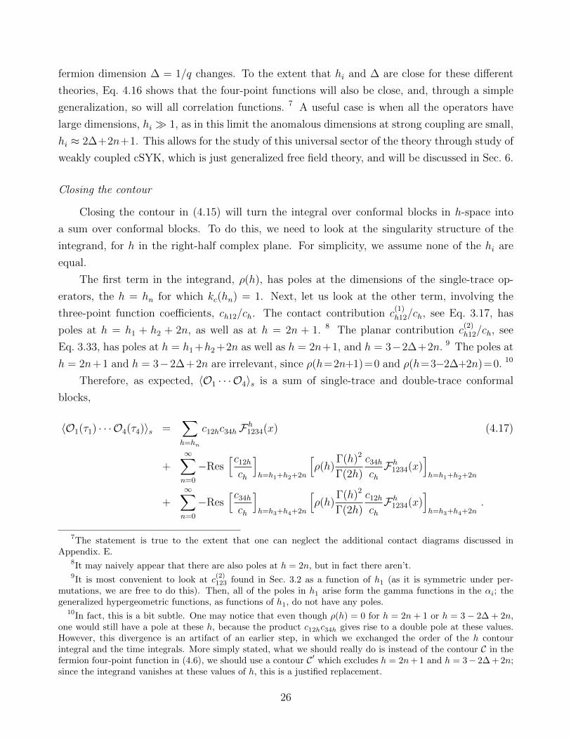
Figure 12: A contribution to the eight-point function. This was included in both lines shownbefore in Fig. 9, and so must be subtracted due to double counting.
Subtracting a planar
The first term on the second line of (4.1) is the diagram shown in Fig. 12. This is similar
to the sum of the s-channel exchange diagrams we already computed, the only difference being
that it only sums planar diagrams, and that instead of the full fermion four-point function Fappearing in the exchange, one has the free fermion four-point function, F0. This allows us to
immediately write the answer,
〈O1(τ1) · · · O4(τ4)〉0s =
∫C
dh
2πi
ρ0(h)
c2h
Γ(h)2
Γ(2h)c
(2)12hc
(2)34hF
h1234(x) . (4.19)
Closing the contour yields a sum of both single-trace and double-trace conformal blocks. The
single-trace blocks are for operators of dimension 2∆ + 2n + 1, which serve to cancel the same
blocks that arise from expanding the exchange diagrams in the cross-channel. The double-trace
blocks are again for operators of the type [O1O2]n and [O3O4]n.
Mellin space
It is sometimes useful to represent the four-point function in Mellin space, see Appendix A.1
for our conventions. In order to find the Mellin transform of 〈O1 · · · O4〉s, denoted by Ms(hi, γ12),
it is most convenient to use the form of the expression in (4.7). The integral appearing there is
denoted by Bh1234 in Appendix A, see Eq. A.10, and its Melin transform, Mh1234(γ12), is given in
(A.23). Therefore Ms(hi, γ12) is the contour integral,
Ms(hi, γ12) =1
2
∫C
dh
2πi
ρ(h)
chc1−hc12h c34 1−h M
h1234(γ12) . (4.20)
Similarly, the Mellin transform of 〈O1 · · · O4〉0s is,
M0s (hi, γ12) =
1
2
∫C
dh
2πi
ρ0(h)
chc1−hc
(2)12h c
(2)34 1−h M
h1234(γ12) . (4.21)
28
1
2
43
5
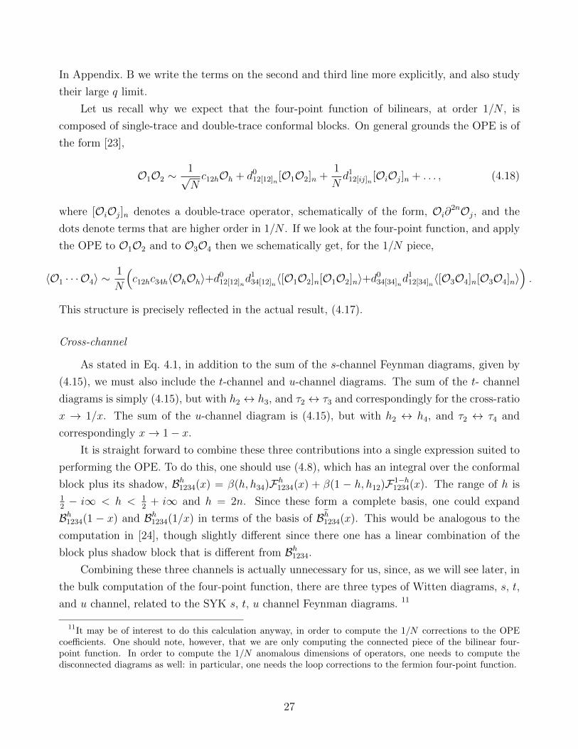
Figure 13: A contribution to the ten-point function.
Due to the complexity of c123, these expressions are not in themselves especially enlightening.
In Sec. 6 we will study the limit of hi � 1, in which the full four-point function, as well as its
Mellin transform, significantly simplify.
5. Higher-Point Correlation Functions
In the previous section we computed the bilinear four-point function. It is straightforward
to generalize to higher-point functions. These will be expressed in terms of contour integrals
involving the ρ(h) from summing ladders in Sec. 2, the c123 computed in Sec. 3, and higher-point
conformal blocks.
For instance, consider a fermion ten-point function. An example of a class of diagrams that
contribute is shown in Fig. 13. To compute such diagrams, we use the same method as in the
previous section, writing the intermediate fermion four-point functions (of which there are now
two) in the form given by Eq. 4.6. The contribution to the bilinear five-point function is then,
〈O1(τ1) · · · O5(τ5)〉s =1
4
∫C
dha2πi
ρ(ha)
chac1−ha
∫C
dhb2πi
ρ(hb)
chbc1−hb∫dτadτb 〈O1(τ1)O2(τ2)Oha(τa)〉〈O1−ha(τa)O3(τ3)Ohb(τb)〉〈O1−hb(τb)O4(τ4)O5(τ5)〉 . (5.1)
The integrals over τa, τb will be evaluated in the next section; the result is a sum of five-point
conformal blocks and their shadows. After changing variables, ha → 1− ha and ha → 1− hb on
some of the terms, similar to what was done in the case of the bilinear four-point function, we
find,
〈O1(τ1) · · · O5(τ5)〉s =
∫C
dha2πi
ρ(ha)
c2ha
Γ(ha)2
Γ(2ha)
∫C
dhb2πi
ρ(hb)
c2hb
Γ(hb)2
Γ(2hb)c12ha
cha 3hbchb 45F
ha,hb12345(x1, x2) ,
(5.2)
29
where Fha,hb12345(x1, x2) is the five-point conformal block, depending on the two cross-ratios of times,
x1 =τ12τ34
τ13τ24
, x2 =τ23τ45
τ24τ35
. (5.3)
The prescription for writing a general connected p-point correlation function 〈Oh1· · · Ohp〉,
to leading nontrivial order in 1/N , is clear. One draws all Feynman-like skeletons, in which the
lines are ladders and there are “cubic interactions” c123 (where c123 is the coefficient of 〈O1O2O3〉found in Sec. 3). For each internal line, one has a contour integral,∫
C
dha2πi
ρ(ha)
c2ha
Γ(ha)2
Γ(2ha). (5.4)
The integrand consists of the “cubic interactions” c123, and a p-point conformal block. One
writes down such an expression for each of the skeleton diagrams. One should then subtract
diagrams with no exchanged melons in some channels, which were over-counted; these have the
same rules but with a ρ0 and a c(2)123 (as was discussed in the four-point function case, Eq. 4.19).
Finally, if q is sufficiently large, there are additional contact diagrams one must add, which
consist of four or more ladders meeting at a melon; these are discussed in Appendix E. From the
correlation functions 〈Oh1· · · Ohp〉, one can obtain the 2p-point fermion correlation function, as
discussed in Appendix D.
5.1. Five-point conformal blocks
In conformal field theories, the functional form of the building blocks of correlation functions
is fully fixed by conformal invariance. As discussed in Appendix A, the OPE takes the form,
O1(τ1)O2(τ2) =∑h
c12h C12h(τ12, ∂2)Oh , (5.5)
where C12h(τ12, ∂2) accounts for descendants of Oh, and is fully determined by the functional
form of the three-point function. The conformal blocks are in turn fully determined by the
C12h(τ12, ∂2). For instance, the four-point block is,
Fh1234(x) = C12h(τ12, ∂2) C34h(τ34, ∂4) 〈Oh(τ2)Oh(τ4)〉 , (5.6)
and the five-point block is,
Fha,hb12345(x1, x2) = C12ha(τ12, ∂2) C45hb
(τ45, ∂4) 〈Oha(τ2)O3(τ3)Ohb(τ4)〉 . (5.7)
30

To determine the higher-point conformal blocks, one simply continues to successively apply the
OPE. See [25] for a recent study, in the context of Virasoro blocks.
An alternative way to obtain an explicit form for the higher-point SL2 conformal blocks is to
simply evaluate the integrals that appear in the higher-point correlation function. For instance,
the expression that appeared in the five-point function is,
Ba,b12345 =
∫dτadτb 〈O1(τ1)O2(τ2)Oha(τa)〉〈O1−ha(τa)O3(τ3)O1−hb(τb)〉〈Ohb(τb)O4(τ4)O5(τ5)〉 ,
where we have changed hb → 1 − hb, relative to (5.1), in order to make the expression more
symmetric. Through a change of variables, we rewrite this so that it is a function of the two
cross-ratios x1, x2 defined in (5.3),
Ba,b12345 =1
|τ12|h1+h2|τ45|h4+h5 |τ34|h3
∣∣∣τ23
τ13
∣∣∣h12∣∣∣τ24
τ23
∣∣∣h3∣∣∣τ35
τ34
∣∣∣h45
Ca,b12345 , (5.8)
where,
Ca,b12345 = |x1|1−ha|x2|1−hb∫dτadτb
|1− τax1 − τbx2|ha+hb+h3−2
|τa|ha−h12|τa − 1|ha+h12|τb|hb+h45|τb − 1|hb−h45. (5.9)
Let us assume 0 < x1, x2 < 1. From the integral definition of the Appell function F2 we notice
that, if our integral were in the range 0 < τa, τb < 1, then Ca,b12345 would be proportional to,
x1−ha1 x1−hb
2 F2
[2−ha−hb−h3 1+h12−ha 1−h45−hb
2−2ha 2−2hb;x1 x2
]. (5.10)
The differential equation defining the Appell function F2 has a total of four solutions, which
follow from (5.10). Our integral Ca,b12345 should be a linear combination of these. We set the
coefficients by studying the integral Ca,b12345 in various limits, similar to what we did for the
integral appearing in the three-point function in Sec. 3.2. The result is expressed in terms of
the five-point conformal blocks,
Fha,hb12345(x1, x2) =1
|τ12|h1+h2|τ45|h4+h5 |τ34|h3
∣∣∣τ23
τ13
∣∣∣h12∣∣∣τ24
τ23
∣∣∣h3∣∣∣τ35
τ34
∣∣∣h45
xha1 xhb2 F2
[ha+hb−h3 ha+h12 hb−h45
2ha 2hb;x1 x2
], (5.11)
31
and is given by,
Ba,b12345 = β(ha, hb+h3−1)β(hb, h3−ha)Fha,hb12345(x1, x2)+β(1−ha, h12)β(hb, ha+h3−1)F1−ha,hb
12345 (x1, x2)
+β(ha, hb+h3−1)β(1−hb, h45)Fha,1−hb12345 (x1, x2)+β(1−ha, h12)β(1−hb, h45)F1−ha,1−hb12345 (x1, x2) ,
where β(h,∆) is defined in Appendix. A, see Eq. A.13. We established which of the four terms
in this expression is identified as the five-point conformal block by looking at the small τ12, τ45
behavior.
One could, in this way, compute six-point blocks and higher, though we will stop here.
6. Generalized Free Field Theory
In the previous sections we gave a prescription for determining all correlation functions in
SYK, 〈Oh1· · · Ohp〉. The operators Oh have small anomalous dimensions when the dimension h is
large, h� 1. As we showed, the correlators of these are determined from the weak coupling limit
of cSYK: generalized free field theory of fermions, and can be found through Wick contraction.
This provides significant simplification.
In this section, we study the generalized free field theory ofN fermions of dimension ∆, in the
singlet sector. In Sec. 6.1 we compute the correlation functions of the primary O(N) invariant
fermion bilinears. Then in Sec. 6.2 and Sec. 6.3 we use saddle point analysis to simplify the
three-point and four-point functions, respectively, in the limit of large hi.
6.1. Wick contractions and generating function
The fermion bilinear, primary, O(N) invariant operators are given by,
On =1√N
N∑i=1
n∑r=0
dn r ∂rτ χi ∂
n−rτ χi , (6.1)
where dn r is,
dn r =(−1)r
Γ(n− r + 1)Γ(∆ + n− r) Γ(r + 1) Γ(∆ + r). (6.2)
Due to fermion antisymmetry, only correlation functions of On involving odd n are nonzero. As
a result, throughout this paper On has been used to denote what in the current language is
O2n+1; for the purposes of this section, the current definition is more convenient.
32
Wick Contractions
The correlation functions of the On follow trivially by Wick contractions. The connected
piece of a p-point correlation function is,
〈On1(τ1) · · · Onp(τp)〉 =
1
Np−2
2
∑r1,...,rp
dn1r1· · · dnprp
(∂np−rpp ∂r11 G(τ1 p)
)×(∂n1−r1
1 ∂r22 G(τ12)) (∂n2−r2
2 ∂r33 G(τ23))· · ·(∂np−1−rp−1
p−1 ∂rpp G(τp−1 p)
)+ perm . (6.3)
Using that dnr = (−1)ndnn−r, one can see that the addition of permutations gives a factor
(1−(−1)n1) · · · (1−(−1)np) multiplying the term we explicitly wrote. Making use of the derivative
of the two-point function,
∂p1 G(τ12) = G(τ12)Γ(2∆ + p)
Γ(2∆)
(−1)p
τ p12
, (6.4)
the p-point function becomes,
〈On1(τ1) · · · Onp(τp)〉 =
1
Np−2
2
(∏i
δni=odd)−(−2)p
Γ(2∆)pG(τ12)G(τ23) · · ·G(τp−1 p) G(τ1p)
∑r1,...,rp
dn1r1· · · dnprp (−1)r2+...rp−1
Γ(2∆ + np − rp + r1)
τnp−rp+r11p
Γ(2∆ + n1 − r1 + r2)
τn1−r1+r212
Γ(2∆ + n2 − r2 + r3)
τn2−r2+r323
· · ·Γ(2∆ + np−1 − rp−1 + rp)
τnp−1−rp−1+rpp−1 p
. (6.5)
Generating function
It is convenient to introduce a generating O(τ, x) which includes all the On(τ), see for
instance [26],
O(τ, x) =∞∑n=0
On(τ)xn . (6.6)
Using the explicit definition of the On in terms of fermions the generating O(τ, x) becomes,
O(τ, x) =1√N
N∑i=1
D(x, τ)χi(τ)D(−x, τ)χi(τ) , (6.7)
33

where we have defined,
D(x, τ) =∞∑r=0
(−x)r
r! Γ(r + ∆)∂rτ = (x∂τ )
1−∆2 J∆−1(2
√x∂τ ) . (6.8)
We now compute the correlation functions of O(τ, x). The two-point function is,
〈O(τ1, x1)O(τ2, x2)〉 = H(x1, τ1,−x2, τ2)H(−x1, τ1, x2, τ2)−H(x1, τ1, x2, τ2)H(−x1, τ1,−x2, τ2)
(6.9)
where
H(x1, τ1, x2, τ2) = D(x1, τ1)D(x2, τ2)G(τ12) . (6.10)
Using the definition of D(xi, τi) and acting with the derivatives on G(τ12), and then using the
integral definition of the Gamma function, performing the sum, and evaluating the resulting
integral, we get,
H(x1, τ1, x2, τ2) =G(τ12)
Γ(2∆)
(x1x2
τ 212
) 1−∆2
ex1−x2τ12 J∆−1
(2
√x1x2
τ 212
). (6.11)
If we insert H into (6.9), and Taylor expand, we recover the two-point functions 〈On(τ1)On(τ2)〉.In the ∆ = 0 limit these are,
〈O(x1, τ1)O(x2, τ2)〉 =1
Γ(2∆)2
∞∑n=1
(x1 x2
τ 212
)2n+1 (Nn
(2n!)
)2
, N2n =
24n+1
(2n+ 1)
Γ(2n+ 12)
√πΓ(2n)
.
(6.12)
In the large n limit these simplify to,(Nn
(2n!)
)2
≈( en
)4n
, n� 1 . (6.13)
A p-point correlation function of the O(τ, x) is a simple generalization of the two-point
function,
〈O(τ1, x1)O(τ2, x2) · · · O(τp, xp)〉 = (6.14)
H(x1, τ1,−xp, τp)H(−x1, τ1, x2, τ2)H(−x2, τ2, x3, τ3) · · ·H(−xp−1, τp−1, xp, τp) + perm .
To obtain the correlators of the Oni , one should Taylor expand the right-hand side, extracting
the coefficient of the xnii term. Upon Taylor expansion, each of the permutations gives the same
contribution, up to a sign, and serves to ensure that the correlation function 〈On1(τ1) · · · Onp(τp)〉
is nonzero only for odd ni.
34
6.2. Asymptotic three-point function
We would like to find the form of the three-point function 〈On1(τ1)On2
(τ2)On3(τ3)〉 in the
limit that n1, n2, n3 � 1. This is simplest to do through study of the correlator
〈O(τ1, x1)O(τ2, x2)O(τ3, x3)〉. 12 Writing this out explicitly,
〈O(x1, τ1)O(x2, τ2)O(x3, τ3)〉 =sgn(τ12τ13τ23)
Γ(2∆)3
∣∣∣x1x2
τ 212
∣∣∣ 1−∆2∣∣∣−x1x3
τ 213
∣∣∣ 1−∆2∣∣∣x2x3
τ 223
∣∣∣ 1−∆2
exp
(x1
τ23
τ12τ13
− x2
τ13
τ12τ23
+ x3
τ12
τ13τ23
)J∆−1
(2
√x1x2
τ 212
)J∆−1
(2
√−x1x3
τ 213
)J∆−1
(2
√x2x3
τ 223
)+ 7 perm. (6.15)
If we were to expand this, it would give, for ∆→ 0,
〈O(x1, τ1)O(x2, τ2)O(x3, τ3)〉 =
1
Γ(2∆)3
∑ x2n1+11
(2n1)!
x2n2+12
(2n2)!
x2n3+13
(2n3)!
8 s(2)n1n2n3
|τ12|2(n1+n2−n3)+1|τ23|2(n2+n3−n1)+1|τ31|2(n3+n1−n2)+1, (6.16)
where s(2)n1n2n3
is a triple sum, see Eq. B.8.
More directly, we can extract the desired correlator through a triple contour integral over
the unit circle,
〈On1(τ1)On2
(τ2)On3(τ3)〉 =
3∏i=1
∮dxi
(2πi)xni+1i
〈O(x1, τ1)O(x2, τ2)O(x3, τ3)〉 . (6.17)
To work with (6.15), we use the following representation of the Bessel function,
Jν(z) =(z
2
)ν ∫L
ds
2πi
1
sν+1 exp
(s− z2
4s
), (6.18)
where the contour L comes in from −∞, circles around the origin, and returns to −∞. With this
representation of the Bessel function, we have 〈On1(τ1)On2
(τ2)On3(τ3)〉 in terms of six-contour
integrals. In the limit of large ni, we may evaluate these by saddle point analysis. We will only
be interested in the dominant term, and will not compute the subleading corrections. Dropping
all terms that are not exponential in the ni, and not distinguishing between ni and ni − 1, we
12 In Sec. 3.2 we found the three-point function by evaluating Feynman diagrams, obtaining an expressionin terms of a generalized hypergeometric function at argument 1; see Eq. B.8 for the expression in the currentcontext. However, since some of the arguments of this hypergeometric function are negative, written as a singlesum, it includes both positive and negative terms, which makes its asymptotic analysis, in this form, difficult.
35
have,
〈On1(τ1)On2
(τ2)On3(τ3)〉≈ sgn(τ12τ13τ23)
Γ(2∆)3
3∏i=1
∫L
dsi2πi
3∏i=1
∮dxi
(2πi)exp
(x1
τ23
τ12τ13
−x2
τ13
τ12τ23
+x3
τ12
τ13τ23
)
exp
(−
3∑i=1
ni log xi + s1 −x2x3
τ 223
1
s1
+ s2 +x1x3
τ 213
1
s2
+ s3 −x1x2
τ 212
1
s3
). (6.19)
Note that, at this level of approximation, it makes no difference what ∆ is. The saddle equations
from varying the si are,
s21 = −x2x3
τ 223
, s22 =
x1x3
τ 213
, s23 = −x1x2
τ 212
. (6.20)
The saddle equations from varying the xi are,
−n1
x1
+x3
τ 213 s2
− x2
τ 212 s3
+τ23
τ12τ13
= 0 (6.21)
−n2
x2
− x3
τ 223 s1
− x1
τ 212 s3
− τ13
τ12τ23
= 0 (6.22)
−n3
x3
− x2
τ 223 s1
+x1
τ 213 s2
+τ12
τ13τ23
= 0 . (6.23)
We multiply the first equation by x1, the second by x2, and the third by x3. We then apply
(6.20) to simplify the left-hand side. This gives,
s2 + s3 = n1 − x1
τ23
τ12τ13
, s1 + s3 = n2 + x2
τ13
τ12τ23
, s1 + s2 = n3 − x3
τ12
τ13τ23
. (6.24)
We now trivially solve for the xi, and insert into (6.20) to get,
s21 = (n2−s1−s3)(n3−s1−s2) , s2
2 = (n1−s2−s3)(n3−s1−s2) , s23 = (n1−s2−s3)(n2−s1−s3) .
Solving gives two solutions. The first is,
s1 =n2n3
n1 + n2 + n3
, s2 =n1n3
n1 + n2 + n3
, s3 =n1n2
n1 + n2 + n3
, (6.25)
and is the dominant saddle, while the second is,
s1 =n2n3
−n1 + n2 + n3
, s2 =n1n3
n1 − n2 + n3
, s3 =n1n2
n1 + n2 − n3
. (6.26)
36

Inserting the dominant saddle into the integrand, we find the three-point function is,
〈On1(τ1)On2
(τ2)On3(τ3)〉 ≈ 1
|τ23|n2+n3−n1|τ13|n1+n3−n2|τ12|n1+n2−n3
(eN)N
n2n11 n2n2
2 n2n33
, n1, n2, n3 � 1 ,
(6.27)
where we defined N = n1 + n2 + n3.
In terms of sn1n2n3, comparing (6.27) with (6.16), we have that,
s(2)n1n2n3
≈ (2N)2N
(2n1)2n1(2n2)2n2(2n3)2n3≈ (2N)!
(2n1)!(2n2)!(2n3)!, n1, n2, n3 � 1 . (6.28)
Equipped with the asymptotic limit of the three-point function, we can find the asymptotic limit
of the cubic couplings of the dual bulk scalars φn dual to O2n+1 [6]. With the φn canonically
normalized, we have,
λn1n2n3≈ N !
Γ(N − 2n1 + 12)Γ(N − 2n2 + 1
2)Γ(N − 2n3 + 1
2), n1, n2, n3 � 1 , (6.29)
where we have, for simplicity, dropped any order-one factors that may have appeared. One
would ultimately like to have a string-like bulk interpretation of these couplings.
6.3. Asymptotic four-point function
To find the behavior of the four-point function 〈On1(τ1) · · · On4
(τ4)〉 for large ni we perform
an analogous analysis as with the three-point function. Representing the four-point function as
a contour integral, and dropping all terms that aren’t exponential, we have,
〈On1(τ1) . . .On4
(τ4)〉 ≈ sgn(τ12τ23τ34τ41)
Γ(2∆)4
4∏i=1
∫L
dsi2πi
4∏i=1
∮dxi
(2πi)
exp
(−x1
τ24
τ12τ14
− x2
τ13
τ12τ23
− x3
τ24
τ23τ34
− x4
τ13
τ14τ34
)exp
(−
4∑i=1
ni log xi + s1 +x1x2
τ 212 s1
+ s2 +x2x3
τ 223 s2
+ s3 +x3x4
τ 234 s3
+ s4 +x4x1
τ 241 s4
). (6.30)
At large ni we can approximate the integral by its saddle. Varying with respect to the si gives
the saddle equations,
s21 =
x1x2
τ 212
, s22 =
x2x3
τ 223
, s23 =
x3x4
τ 234
, s24 =
x4x1
τ 241
. (6.31)
37
Varying, in addition, with respect to xi gives the saddle equations,
−n1
x1
+x2
τ 212 s1
+x4
τ 241 s4
− τ24
τ12τ14
= 0 (6.32)
−n2
x2
+x1
τ 212 s1
+x3
τ 223 s2
− τ13
τ12τ23
= 0 (6.33)
−n3
x3
+x2
τ 223 s2
+x4
τ 234 s3
− τ24
τ23τ34
= 0 (6.34)
−n4
x4
+x3
τ 234 s3
+x1
τ 241 s4
− τ13
τ14τ34
= 0 . (6.35)
We multiply the first equation by x1, the second by x2, and so on, and use (6.31) to simplify,
s4 + s1 = n1 +τ24
τ12τ14
x1 , s1 + s2 = n2 +τ13
τ12τ23
x2 , (6.36)
s2 + s3 = n3 +τ24
τ23τ34
x3 , s3 + s4 = n4 +τ13
τ14τ34
x4 .
Now, using the saddle equations, at the saddle we see that the four-point function is,
〈On1(τ1) . . .On4
(τ4)〉 ≈ 1∏i x
nii
exp(∑
ni
)(6.37)
Trivially solving (6.36) for the xi and inserting into (6.31) gives, in terms of the cross-ratio
x = τ12τ34
τ13τ24,
s21 = (1− x)(s4 + s1 − n1)(s1 + s2 − n2) (6.38)
s22 = x(s1 + s2 − n2)(s2 + s3 − n3)
s23 = (1− x)(s2 + s3 − n3)(s3 + s4 − n4)
s24 = x(s3 + s4 − n4)(s4 + s1 − n1) .
The solution to these equations for general ni is complicated. A simple case, which we focus on,
is when all of the dimensions ni are equal.
Equal ni
We set n1 = n2 = n3 = n4. In this case we can simplify (6.37) to,
〈On1(τ1) . . .On1
(τ4)〉 ≈ exp(4n)1
(τ 212τ
223τ
234τ
241s
21s
22s
23s
24)
n2
, n1 � 1 . (6.39)
38
The symmetric product of the times can alternatively be written as,
τ 212τ
223τ
234τ
241 = τ 4
12τ434
(1− xx
)2
. (6.40)
We define si = si/n1. Then, since (n/e)n ≈ n!,
〈On1(τ1) . . .On1
(τ4)〉 ≈ 1
(n1!)4
1
(τ 212τ
234)n1
1((1−x)xs1s2s3s4
)n1, n1 � 1 . (6.41)
To complete the evaluation of the four-point function we need to solve (6.38) for the si, and
insert their product into (6.41). There are eight solutions to (6.38). In writing them, we assume
that we have a time-ordered correlation function, so that cross-ratio of times is in the range
0 < x < 1. The other time orderings can be worked out in a similar fashion. Of the eight saddle,
two saddles give the product,
s1s2s3s4 =x− 1
16x. (6.42)
Another two saddles give,
s1s2s3s4 =x
16(x− 1), (6.43)
while the remaining four saddles give,
s1s2s3s4 =x(1− x)
(1±√x±√
1− x)4 . (6.44)
The dominant saddle, for all values of 0 < x < 1, is clearly the one for which,
s1s2s3s4 =x(1− x)
(1 +√x+√
1− x)4 . (6.45)
Inserting this into (6.41), we have,
〈On1(τ1) . . .On1
(τ4)〉 ≈ −1
(τ 212τ
234)n1
((√x+√
1− x+ 1)4
(1− x)2
)n1 1
(n1!)4 , n1 � 1 . (6.46)
As we cross the boundaries: x = 0 or x = 1, we observe the Stokes phenomenon: the
dominant saddle changes. This means that if we want to consider the limit of x→ 0, or x→ 1,
we must account for multiple saddles. This can already be seen from (6.46) since, by itself, it
has incorrect small x behavior. In particular, expanding around small x gives rises to powers
xm/2, however the single-trace and double-trace operators appearing in the OPE have integer
dimension, so there should not be any terms with odd m. If we were to include one of the other
39
saddles,
s1s2s3s4 =x(1− x)
(1−√x+√
1− x)4 , (6.47)
and have it come with the same phase, then this would eliminate the odd m in the expansion.
Of course, to actually determine the phase one should compute fluctuations about the saddle,
which we have not done.
Mellin transform
It is sometimes useful to study the four-point function in Mellin space, reviewed in Ap-
pendix A.1. In terms of the variables u = x2 and v = (1 − x)2, the four-point function (6.46)
is,
〈On1(τ1) . . .On1
(τ4)〉 =1
(n1!)4
−1
(τ 213τ
224)n1
((u1/4 + v1/4 + 1)4
uv
)n1
. (6.48)
Notice that, since u and v are not independent, we could have written this in other ways. This
ambiguity reflects the non-uniqueness of the Mellin amplitude for CFT1 four-point functions.
However, the choice we made is natural because it is symmetric. Using the standard Mellin-
Barnes representation, we can write,
((u1/4 + v1/4 + 1)4
uv
)n1
=1
(uv)n1
1
Γ(−4n1)
∫ds
2πi
∫dt
2πiΓ(−4n1 + s+ t)Γ(−s)Γ(−t) (u
14 )s(v
14 )t ,
(6.49)
and comparing with (A.22), we find the Mellin amplitude is,
M(γ12, γ14) =−1
(n1!)4
16
Γ(−4n1)
Γ(4n1 − 4γ12 − 4γ14)Γ(4γ12 − 4n1)Γ(4γ14 − 4n1)
Γ(n1 − γ12 − γ14)2Γ(γ12)2Γ(γ14)2 . (6.50)
For a CFT1 four-point function, it would seem more natural to consider a Mellin amplitude
that is a function of only one variable. The reason for studying a two variable Mellin amplitude
is because this is natural from the AdS2 perspective, as will be discussed in the next section.
40

(a) (b)
+ + +
(c)
Figure 14: The Witten diagrams for the AdS computation of CFT correlation functions of O.The (a) two-point function (b) three-point function and (c) four-point function.
7. Bulk
7.1. Constructing the bulk
The bilinear, primary, O(N) invariant singlets On are, via the AdS/CFT dictionary, dual
to scalar fields φn in AdS2. Knowing all large N connected correlation functions of the On, in
principle, fully fixes the classical bulk Lagrangian of the AdS dual of SYK.
On general grounds, we expect the bulk Lagrangian, up to order 1/N , to take the form,
Sbulk =
∫d2x√g
[1
2(∂φn)2 +
1
2m2nφ
2n +
1√Nλnmk φnφmφk
+1
N
(λ0nmkl φnφmφkφl + λ1
nmkl ∂φn∂φmφkφl + . . .)]
. (7.1)
We have not included cubic interaction terms with derivatives, as these can be eliminated through
field redefinitions [6]. At the quartic level, it is no longer possible to eliminate derivatives, and
indeed there should generically be an infinite number of independent quartic terms, with various
combinations of derivatives.
To establish the coefficients appearing in Sbulk, one should use this bulk action to compute
CFT correlation functions, and fix the coefficients so as to match the SYK correlation functions.
This is simple to do for the two-point and the three-point functions, as their functional form
is fixed by conformal invariance. Evaluating the Witten diagram for the two-point function,
Fig. 14(a), gives the standard relation between the mass of φn and the dimension of On, m2n =
hn(hn − 1). From the Witten diagram for the three-point function, Fig. 14(b), one obtains
a simple relation between the cubic coupling λnmk and the coefficient of the SYK three-point
41

function, cnmk.
Starting with the four-point function, the mapping is more involved. Conformal invariance
restricts the four-point function to be a function of the cross-ratio, but is insufficient to fix
the functional form. As result, matching between bulk and boundary requires matching two
functions, rather than just two numbers. In particular, on the bulk side, computation of the
four-point function involves summing over the exchange and contact Witten diagrams, shown
in Fig. 14(c). One must sum over all exchange diagrams: in each of the three channels there is
one for each exchanged φn. One must also sum over all contact Witten diagrams, accounting
for the generically infinite number of quartic terms appearing in the bulk Lagrangian.
One way of organizing the four-point function is by expanding each of the Witten diagrams
as a sum of conformal blocks, and similarly for the SYK four-point function, and then adjusting
the bulk couplings so as to make the coefficients of all blocks match. The matching of the
single-trace blocks is automatic, as these only depend on the cubic couplings. In particular,
the s-channel Witten diagrams, expanded in terms of s-channel blocks, will contain single-trace
blocks whose coefficients will match the coefficients of the single-trace blocks coming from the
sum of s-channel SYK Feynman diagrams, that were computed in Sec. 4.3. The same holds for
the t-channel and u-channel. The matching of coefficients of double-trace blocks is where the
challenge lies: both the exchange and contact Witten diagrams will contain double-trace blocks,
so one must adjust the quartic couplings in order for the total coefficients of the double-trace
blocks to match the SYK result. An approach of this type has been pursued in [27–29], in the
context of the duality between the free O(N) model and Vasiliev theory.
A more tractable way of constructing the bulk at the quartic level, at least for local bulk
theories of a few fields, is to study the four-point function in Mellin space. As discussed in [30],
a contact Witten diagram has a Mellin amplitude that is a polynomial in the Mellin variables,
whose order is set by the number of derivatives in the quartic interaction. In previous sections
we wrote the SYK four-point function in Mellin space, so one could study it further in this
context. The simplest limit is when all four operators have equal and large dimension, in which
case the Mellin amplitude takes the form (6.50). This does not have a natural interpretation
as a polynomial, nor should we have expected it to, if the bulk Lagrangian has terms with an
arbitrarily large number of derivatives, and moreover, no large gap. We leave an analysis of the
bulk at the quartic level to future work: it is likely that the bulk theory should be regarded
as a theory of extended objects, rather than local fields. So one should understand the CFT
four-point function in this context instead.
The only thing that we will do in the rest of the section is analyze further the exchange
Witten diagrams and relate them to SYK exchange Feynman diagrams.
42

7.2. Preliminaries
We begin by collecting some relevant equations for AdS2 computations of correlation func-
tions. The discussion follows [30], with the notational exception that there h denotes one-half
of the boundary spacetime dimension, whereas for us the boundary spacetime dimension is one
and h denotes the operator dimension.
Letting X denote a bulk coordinate and P a boundary coordinate, both in embedding space,
the bulk-boundary propagator is,
Gh(X,P ) =Ch
(−2P ·X)h, where Ch =
Γ(h)
2√π Γ(h+ 1
2). (7.2)
Correspondingly, this leads to a CFT two-point function,
〈Oh(P1)Oh(P2)〉 =Ch
(−2P1 · P2)h, (7.3)
where, upon converting from embedding space to physical space, −2P1 · P2 = (τ1 − τ2)2.
Consider a cubic bulk interaction with coupling equal to one, φ1φ2φ3, involving fields φi dual
to operators Oi of dimension hi. The corresponding tree-level Witten diagram determining the
CFT three-point function involves a product of three bulk-boundary propagators, see Fig. 14(b),
〈O1(P1)O2(P2)O3(P3)〉 =
∫AdS
dX Gh1(X,P1)Gh2
(X,P2)Gh2(X,P3) . (7.4)
Evaluation of the integral gives,
〈O1(P1)O2(P2)O3(P3)〉 =ΛB∂(h1, h2, h3)
(−2P2 · P3)h2+h3−h1
2 (−2P1 · P3)h1+h3−h2
2 (−2P1 · P2)h1+h2−h3
2
, (7.5)
where,
ΛB∂(h1, h2, h3) =Γ(h1+h2+h3−1
2
)Γ(h2+h3−h1
2
)Γ(h1+h3−h2
2
)Γ(h1+h2−h3
2
)16πΓ(h1 + 1
2)Γ(h2 + 1
2)Γ(h3 + 1
2)
. (7.6)
As a result, the relation between the cubic couplings λ123 and the coefficients c123 of the CFT
three-point function is,
λ123 =c123
ΛB∂(h1, h2, h3)
√C1C2C3 , (7.7)
where the Ci appear due to the CFT convention of two-point functions having norm equal to
one.
43

Figure 15: A convenient way to evaluate an exchange Witten diagram is to make use of thesplit-representation of the bulk two-point function.
For computing exchange Witten diagrams, we will need the bulk propagator for a field dual
to an operator of dimension h,
GhBB(X, Y ) =
Γ(h)
2√πΓ(h+ 1
2)u−h2F1(h, h, 2h,−4
u) , (7.8)
where u = (X − Y )2. One can verify the following representation of the propagator minus the
“shadow” propagator, written in terms of two bulk-boundary propagators,∫∂AdS
dP0 Gh(P0, X)G1−h(P0, Y ) =1
(1− 2h)
(GhBB(X, Y )−G1−h
BB (X, Y )). (7.9)
One may notice the similarity between (7.8) and the CFT1 conformal blocks, and between (7.9)
and the representation of the conformal block plus its shadow as a product of a three-point
function involving Oh and a three-point function involving its shadow, see Appendix A. This
similarity will be utilized later, in connecting boundary Feynman diagrams to bulk Witten
diagrams. Performing a contour integral of (7.9) over h gives the standard split-representation,
GhBB(X, Y ) =
∫dhc2πi
2(hc − 12)2
(hc − h)(hc − 1 + h)
∫∂AdS
dP0 Ghc(X,P0)G1−hc(Y, P0) , (7.10)
where the hc integral runs parallel to the imaginary axis, 12− i∞ < hc <
12
+ i∞. Finally, a delta
function in AdS can also be written in terms of a split-representation, with the same contour,
δ(X − Y ) = −2
∫dhc2πi
(hc −1
2)2
∫∂AdS
dP0 Ghc(X,P0)G1−hc(Y, P0) . (7.11)
44
7.3. Exchange Witten diagrams
Consider an s-channel exchange diagram, shown in Fig. 15, where a field dual to an operator
of dimension h is exchanged. This is given by,
Ws =
∫dXdY Gh1
(τ1, X)Gh2(τ2, X)Gh
BB(X, Y )Gh3(τ3, Y )Gh4
(τ4, Y ) . (7.12)
In Appendix. F we evaluate this; using the split-representation for the bulk propagator gives a
nice form in terms of single-trace and double-trace conformal blocks. For the bulk dual of SYK,
since the bulk theory contains a whole tower of fields, we must sum over all the φh, dual to Oh,that can be exchanged, requiring us to evaluate,
〈O1O2O3O4〉s =∑h=hn
c12h
ΛB∂(h1, h2, h)
c34h
ΛB∂(h3, h4, h)Ch∫
dXdY Gh1(τ1, X)Gh2
(τ2, X)GhBB(X, Y )Gh3
(τ3, Y )Gh4(τ4, Y ) , (7.13)
where we have made use of the expression (7.7) relating the cubic couplings to the SYK three-
point function coefficients. The sum is over all the physical Oh in the theory; in particular the
h > 0 that satisfy the transcendental equation, kc(h) = 1 given in (2.11). The most direct way
to evaluate this would be to use the expression in Appendix. F for a single Witten diagram
expressed as a single-trace conformal block and a sum of double-trace blocks, see Eq. F.4, and
then evaluate the sum over all the operators hn. This will yield a sum of single-trace and double-
trace blocks. The coefficients of the single-trace blocks will clearly be the same as what was found
for SYK s-channel exchange diagrams, c12hc34h, see Eq. 4.17. The coefficients of the double-trace
blocks, however, will be complicated. In what follows, we will perform some manipulations to
simplify them.
An important step is to start by replacing the sum over the dimensions of the exchanged
operators with a contour integral,
〈O1O2O3O4〉s =
∫C
dh
2πi
ρ(h)
c2h
Γ(h)2
Γ(2h)
c12h
ΛB∂(h1, h2, h)
c34h
ΛB∂(h3, h4, h)Ch∫
dXdY Gh1(τ1, X)Gh2
(τ2, X)GhBB(X, Y )Gh3
(τ3, Y )Gh4(τ4, Y ) . (7.14)
To verify that this step is correct, we should check that if we close the contour in (7.14) we
get back to (7.13). In particular, the integrand in (7.14) should not have any poles except at
those h equal to the physical dimensions, kc(h) = 1, and moreover, for these h the residue of
the poles should agree with what is in (7.13). The latter property is clearly satisfied, due to the
45

definition of c2h in terms of the residue of ρ(h), (2.28). To check the former, that there are no
additional poles, recall the analytic structure of c12h/ch, discussed at the end of Sec. 4.3. For h
in the right-half complex plane, the only poles we need to potentially be concerned about are at
h = h1 +h2 +2n, however ΛB∂(h1, h2, h) also has poles at these h, so the ratio c12h/ΛB∂(h1, h2, h)
is finite at h = h1 + h2 + 2n. Thus, we are justified in going from (7.13) to (7.14).
Proceeding, we make use of the property (4.12) relating c12h to c12 1−h to note that,
ch c12 1−h
c1−h c12h
ΛB∂(h1, h2, h)
ΛB∂(h1, h2, 1− h)=
Γ(h2)2Γ(3
2− h)
Γ(1−h2
)2Γ(12
+ h). (7.15)
One can verify this implies the following identity,
1
2
1
(1− 2h)
(ch c34 1−h
c1−h c34h
ΛB∂(h3, h4, h)
ΛB∂(h3, h4, 1− h)+ρ(1− h)
ρ(h)
ch c12 1−h
c1−h c12h
ΛB∂(h1, h2, h)
ΛB∂(h1, h2, 1− h)
)= Ch
Γ(h)2
Γ(2h).
Inserting this identity into (7.14) we get,
〈O1O2O3O4〉s =
∫C
dh
2πi
ρ(h)
c2h
c12h
ΛB∂(h1, h2, h)
c34h
ΛB∂(h3, h4, h)
1
2
1
(1− 2h)
(ch c34 1−h
c1−h c34h
ΛB∂(h3, h4, h)
ΛB∂(h3, h4, 1− h)+ρ(1− h)
ρ(h)
ch c12 1−h
c1−h c12h
ΛB∂(h1, h2, h)
ΛB∂(h1, h2, 1− h)
)∫dXdY Gh1
(τ1, X)Gh2(τ2, X)Gh
BB(X, Y )Gh3(τ3, Y )Gh4
(τ4, Y ) . (7.16)
Recall that the contour C has two pieces: a line parrallel to the imaginary axis, and circles
around even integers, as was shown in Fig. 4. Let us focus on the contribution of the line piece.
For this, we may change variables h→ 1− h for the second term to get,
〈O1O2O3O4〉s ⊃∫dXdY Gh1
(τ1, X)Gh2(τ2, X)Gh3
(τ3, Y )Gh4(τ4, Y )∫
h= 12
+is
dh
2πi
ρ(h)
chc1−h
c12h
ΛB∂(h1, h2, h)
c34 1−h
ΛB∂(h3, h4, 1− h)
1
2
1
(1− 2h)
(GhBB(X, Y )−G1−h
BB (X, Y )).
Recalling the representation of the bulk two-point function minus its shadow, as given in (7.9),
we rewrite this as,
〈O1O2O3O4〉s ⊃1
2
∫h= 1
2+is
dh
2πi
ρ(h)
chc1−h
c12h
ΛB∂(h1, h2, h)
c34 1−h
ΛB∂(h3, h4, 1− h)∫dXdY dτ0Gh1
(τ1, X)Gh2(τ2, X)Gh3
(τ3, Y )Gh4(τ4, Y )Gh(τ0, X)G1−h(τ0, Y ) . (7.17)
46
Recognizing that the integral over X of three bulk-boundary propagators is what appears in the
cubic Witten diagram, (7.4), and similarly for the integral over Y , we finally have,
〈O1O2O3O4〉s ⊃1
2
∫h= 1
2+is
dh
2πi
ρ(h)
chc1−h
∫dτ0〈O1(τ1)O2(τ2)Oh(τ0)〉〈O3(τ3)O4(τ4)O1−h(τ0)〉 .
This precisely matches the analogous SYK answer, (4.7), for the s-channel exchange Feynman
diagrams, for the contribution of the line piece of the contour.
If we suppose, for the moment, that the contour C necessary for a complete basis of conformal
blocks in a one-dimensional CFT consisted only of the line parallel to the imaginary axis (and did
not also require circles around positive even integers), then the above would have demonstrated
that the sum over all s-channel exchange Feynman diagrams in SYK (Fig. 2) is equal to the
sum over all s-channel exchange Witten diagrams. This would be a remarkably simple result.
Furthermore, it would imply that the SYK Feynman diagrams with no exchanged melons, Fig. 12,
are dual to the sum over all contact Witten diagrams.
Unfortunately, we must also include the contribution of the contour in (7.14) coming from
circles wrapping h = 2n. Here we can not change variables, so as to form the combination of
the bulk propagator and its shadow needed to apply (7.9). We can of course use the expression
for an individual Witten diagram as a sum of conformal blocks, and then sum over the h = 2n.
This will give the same single-trace piece as in the SYK s-channel exchange diagrams answer,
as it must, but there will be additional double-trace terms (which, aside from simplicity, we had
no reason not to expect).
8. Discussion
The conformal symmetry of SYK at strong coupling fully fixes the functional form of the
building blocks of all correlation functions. The dynamical information in the fermion two-point,
four-point, and six-point functions is captured by ∆, ρ(h), and c123, respectively. All higher-point
functions are built out of these ingredients.
The structure of c123 is remarkable. Viewed as a function of, for instance, h3, it has poles
at precisely h3 = h1 + h2 + 2n. These poles give rise to the double-trace blocks in the bilinear
four-point function. This is presumably a general result for large N conformal field theories:
that the analytic continuation of a three-point function of scalar operators of dimensions hi has
poles at hi = hj + hk + 2n, where i, j, k are distinct and chosen from 1, 2, 3. 13 It is essential
that there be no additional poles, with the exception of those at the h3 for which ρ(h3) = 0,
13A simple CFT three-point function is the one obtained by computing the Witten diagram for scalars withcubic interaction φ1φ2φ3. This yields (7.6), which indeed has poles at hi = hj + hk + 2n.
47

or else the bilinear four-point function would have the wrong structure. Furthermore, the c123
are analytic functions of hi and ∆, and lead to universality: to the extent that two theories
in the SYK family have similar dimensions hi and ∆, be they SYK at different q or cSYK at
different couplings, the c123, and by extension, all higher-point functions (not accounting for the
additional contact diagrams in Appendix. E), will be similar. The large dimension bilinears have
small anomalous dimensions. As a result, their correlators are well approximated by those of
cSYK at weak coupling: generalized free field theory of fermions of dimension ∆, in the singlet
sector.
Knowing all large-N CFT correlation functions, in principle, determines the full tree-level
AdS dual Lagrangian. However, thinking of the bulk as a collection of fields φn, dual to the
On, with some particular masses and couplings, is not the optimal language: there should be
a string-like interpretation of the bulk, which still needs to be formulated. The place to start
understanding the bulk is with the correlators of the large dimension operators: the interactions
of the very massive bulk fields. We gave a simple expression for the cubic couplings of these.
There is a vague resemblance to string theory: a three-point function of vertex operators for
massive string modes comes with combinatorial factors, as a result of the derivatives. The
four-point function of four equal and large dimension On is also simple, and should have some
string-like interpretation. We hope to report on this in future work.
Acknowledgements
We thank O. Aharony, A. Gadde, T. Hartman, M. Isachenkov, K. Jensen, J. Kaplan, I. Klebanov,
J. Maldacena, J. Penedones, E. Perlmutter, D. Poland, and B. van Rees for helpful discussions.
This work was supported by NSF grant 1125915.
A. Conformal Blocks
Let Oi be CFT1 operators of dimensions hi. Performing an OPE expansion,
O1(τ1)O2(τ2) =∑h
c12hC12h(τ12, ∂2)Oh , (A.1)
where c12h are the OPE coefficients, and the function C12h(τ12, ∂2) is present in order to include
the contributions of all the decedents of Oh. The functional form of C12h(τ12, ∂2) is fully fixed
by conformal invariance: SL(2, R) for a CFT1. In particular, applying the OPE to the first two
48
operators in a three-point function gives,
〈O1(τ1)O2(τ2)O3(τ3)〉 = c123 C123(τ12, ∂2)〈O3(τ2)O3(τ3)〉 . (A.2)
The function C123(τ12, ∂2) can now be found in an explicit form, through Taylor expansion, in
powers of τ12, of the conformal three-point function on the left-hand side of the above,
C123(τ12, ∂2)1
|τ23|2h3=
|τ12|h3−h1−h2
|τ13|h1+h3−h2|τ23|h2+h3−h1=|τ12|h3−h1−h2
|τ23|2h3
(1 + (h2 − h1 − h3)
τ12
τ23
+ . . .).
(A.3)
Equipped with C123(τ12), through successive application of the OPE, the functional form of the
building blocks of any correlation function is fixed. In particular, consider a four-point function,
and apply the OPE either once or twice,
〈O1(τ1)O2(τ2)O3(τ3)O4(τ4)〉 =∑h
c12hC12h(τ12, ∂2)〈Oh(τ2)O3(τ3)O4(τ4)〉 (A.4)
=∑h
c12hc34hC12h(τ12, ∂2) C34h(τ34, ∂4)1
|τ24|2h. (A.5)
The conformal blocks are identified as the functions appearing in the latter expansion,
Fh1234(x) ≡ C12h(τ12, ∂2) C34h(τ34, ∂4)1
|τ24|2h, (A.6)
so that,
〈O1(τ1)O2(τ2)O3(τ3)O4(τ4)〉 =∑h
c12hc34hFh1234(x) . (A.7)
The explicit functional form of the conformal blocks is in terms of a hypergeometric function
[31], 14
Fh1234(x) =∣∣∣τ24
τ14
∣∣∣h12∣∣∣τ14
τ13
∣∣∣h34 1
|τ12|h1+h2|τ34|h3+h4xh 2F1(h− h12, h+ h34, 2h, x) , (A.8)
where hij ≡ hi − hj and x is the conformal cross-ratio,
x =τ12τ34
τ13τ24
. (A.9)
A simple alternative way of deriving the conformal blocks is through the shadow formalism
14The notation, Fh1234(x), is somewhat inaccurate, because as a result of the prefactors, the conformal blocks
are really functions of all the times, not just x.
49

[32,33], see also [16,34]. For an operator Oh having dimension h, its shadow O1−h has dimension
1−h. Consider the integral of a product of a three-point function involving Oh and a three-point
function involving O1−h,
Bh1234 =
∫dτ0 〈O1(τ1)O2(τ2)Oh(τ0)〉〈O1−h(τ0)O3(τ3)O4(τ4)〉
=
∫dτ0
|τ12|h−h1−h2
|τ10|h+h12|τ20|h−h12
|τ34|1−h−h3−h4
|τ30|1−h+h34|τ40|1−h−h34. (A.10)
After a change of variables this becomes,
Bh1234 =1
|τ12|h1+h2
1
|τ34|h3+h4
∣∣∣τ24
τ14
∣∣∣h12∣∣∣τ14
τ13
∣∣∣h34
∫dτ0
|1− x|h12−h34|x|h
|τ0|h−h12|τ0 − x|h+h12 |τ0 − 1|1−h−h34. (A.11)
Evaluating the integral gives a sum of a conformal block of an exchanged Oh and a conformal
block of its shadow,
Bh1234 = β(h, h34)Fh1234(x) + β(1− h, h12)F1−h1234(x) , (A.12)
where we defined,
β(h,∆) =√π
Γ(h+∆2
)Γ(h−∆2
)
Γ(1−h+∆2
)Γ(1−h−∆2
)
Γ(12− h)
Γ(h). (A.13)
In evaluating the integral, we have taken the cross-ratio to be in the range 0 < x < 1. Through
a simple change of variables, one can obtain Bh1234 for other ranges of x as well.
In the special case that the four external operators are fermions with dimension ∆, this
kind of integral was encountered in the SYK fermion four-point function, see Eq. 2.12, in which
case Ψh(x) was defined as,
2
|τ12|2∆|τ34|2∆Ψh(x) = β(h, 0)Fh∆(x) + β(1− h, 0)F1−h
∆ (x) , (A.14)
where Fh∆(x) denotes the conformal block (A.8) with hi = ∆,
Fh∆(x) =sgn(τ12) sgn(τ34)
|τ12|2∆|τ34|2∆xh 2F1(h, h, 2h, x) . (A.15)
Since we are dealing with fermions, we have added an antisymmetry factor of sgn(τ12)sgn(τ34)
relative to the definition in (A.8).
50
A.1. Mellin space
Mellin space is useful for large N CFTs [35, 30]. The Mellin amplitude M(γij) for a four-
point function is defined by,
〈O1(τ1) · · · O4(τ4)〉 =
∫[dγ]
2πiM(γij)
∏i<j
Γ(γij)
(τ 2ij)
γij, (A.16)
where the γij have the constraints,
4∑j=1
γij = 0 , γij = γji , γii = −hi , (A.17)
and the integral [dγ] is over two independent γij, which we will take to be γ12 and γ14. Solving
the constraints for the others,
γ13 = h1 − γ12 − γ14 , γ23 =−h12 + h34
2+ γ14 (A.18)
γ24 =h1 + h2 − h3 + h4
2− γ12 − γ14 , γ34 =
−h13 − h24
2+ γ12 . (A.19)
The four-point function can therefore be written as,
〈O1(τ1) · · · O4(τ4)〉 =(τ 2
23)h12−h34
2
(τ 213)h1
(τ 234)
h13+h242
(τ 224)
h1+h2−h3+h42
∫dγ12
2πi
dγ14
2πiM(γ12, γ14)
∏i<j
Γ(γij) u−γ12v−γ14 ,
(A.20)
where,
u =τ 2
12τ234
τ 213τ
224
= x2 , v =τ 2
14τ223
τ 213τ
224
= (1− x)2 . (A.21)
We see that, unlike in dimensions greater than one, in one dimension the cross-ratios u and v
are not independent. This leads to the non-uniqueness of the four-point Mellin amplitude. In
higher dimensions, the p-point Mellin amplitude is also not unique, for p > d + 2. In the case
that all the operators have the same external dimension, h1 = h2 = h3 = h4, the four-point
function simplifies to,
〈O1(τ1) · · · O1(τ4)〉= 1
(τ 213τ
224)h1
∫dγ12
2πi
dγ14
2πiM(γ12, γ14) Γ(γ12)2Γ(γ14)2Γ(h1−γ12−γ14)2 u−γ12v−γ14 .
(A.22)
In order to find the Mellin transform of a general four-point function, it is convenient to
have the Mellin transform of a conformal block plus its shadow, Bh1234. We will denote this by
Mh1234(γ12, γ14). A simple way to find Mh
1234 is to start with the integral definition of Bh1234 (A.10)
51

and evaluate it through the standard Mellin-Barnes technique. After an appropriate change of
variables, it can be brought into the form (A.16), with,
Mh1234(γ12, γ14) =
π12
Γ(h+h12
2)Γ(h−h12
2)Γ(1−h+h34
2)Γ(1−h−h34
2)
Γ(γ12 + h−h1−h2
2)
Γ(γ12)
Γ(γ12 + 1−h−h1−h2
2)
Γ(γ12 − h13+h24
2)
.
(A.23)
B. Large q Limit
In this appendix we study the large q limit of the three-point and four-point functions. As
a result of the fermions having a small anomalous dimension in the infrared, ∆ = 1/q, there are
some simplifications.
For q � 1, the dimensions of the On approach their free-field values, 2n+ 1,
hn = 2n+ 1 + 2εn , εn =1
q
2n2 + n+ 1
2n2 + n− 1, n ≥ 1 , q � 1 , (B.1)
while the OPE coefficients in the large q limit behave as,
c2n = ε2n
n(1 + 2n)
(n(1 + 2n) + 1) (n(1 + 2n)− 1)
√πΓ(2n+ 1)
Γ(2n+ 12)24n−2 , q � 1 . (B.2)
Three-point function
The contact diagram contribution to the three-point function 〈O1O2O3〉 has a coefficient
that was denoted by c(1)123, given in (3.17), c
(1)123 = c1c2c3 I
(1)123, where I(1)
123 was given in (3.15).
Inserting (B.1) into I(1)123 and expanding to leading order in ε gives [6],
I(1)123 = 2s
(1)123
εn1+ εn2
+ εn3
εn1εn2εn3
, q � 1 , (B.3)
where s(1)123 is,
s(1)123 =(−4)n1+n2+n3
Γ(12+ n2+n3−n1)Γ(1
2+ n1+n3−n2)Γ(1
2+ n1+n2−n3)Γ(1+ n1+n2+n3)
π32 Γ(1 + 2n1)Γ(1 + 2n2)Γ(1 + 2n3)
.
(B.4)
The planar diagram contribution to the three-point function has a coefficient that was denoted
by c(2)123, given in (3.33) as c
(2)123 = c1c2c3 ξ(h1)ξ(h2)ξ(h3) I(2)
123, where I(2)123 ≡ I
(2)123(z = 1) was given
in (3.30). Taking the large q limit this simplifies. Defining
ε± = ε±∆ , (B.5)
52

the factor, ξ(hn) simplifies to,
ξ(hn) =ε−nεn
(n+1
2) , q � 1 , (B.6)
while the expression for I(2)123 simplifies to,
I(2)123 = s
(2)123
(2
(ε+1 + ε−2 )(ε+2 + ε−3 )(ε+3 + ε−1 )
ε+1 ε−1 ε
+2 ε−2 ε
+3 ε−3
− 1
ε+1 ε+2 ε
+3
− 1
ε−1 ε−2 ε−3
), q � 1 , (B.7)
where we are using the short hand εi ≡ εni , and s(2)123 is,
s(2)123 =
(2n1 + 2n2 − 2n3)!(2n2 + 2n3 − 1)!
(2n1 − 1)!(2n2 − 1)!(2n3 − 1)!(1 + 2n2 − 2n3)! 4F3
[1−2n1 2+2n1 1−2n3 −2n3
2 1−2n2−2n3 2+2n2−2n3
; 1
].
(B.8)
In writing it in this form we have assumed n1 > n2 > n3. Using the definition of 4F3, this may be
written as a single finite sum. Previously, in [6], we found (B.7) without taking the large q limit
of the exact answer, but rather by evaluating the integral I(2)123 to leading order in 1/q. There we
noted that s(2)123 is the same expression that appears in computing the three-point function in a
generalized free field theory with fermions of dimension ∆, in the limit ∆→ 0. Specifically (see
Eq. 6.14),
s(2)123 = −
∑p1,p2,p3
(2n1
p1
)(2n2
p2
)(2n3
p3
)(2n1+p2−p1
p2 + 1
)(2n2+p3−p2
p3 + 1
)(2n3+p1−p3
p1 + 1
)zp1−p2+2n2−2n3
(−1−z)p3−p2+2n1−2n3,
(B.9)
where z is a cross ratio of times; the answer is independent of z. While it is not manifest that
(B.8) and (B.9) are the same, one can verify that they are.
Four-point function
The s-channel contribution to the four-point function was given in (4.17). The only term
that was not explicitly stated there is the residue of ch12/ch at h = h1 + h2 + 2n. This consists
of two terms, coming from ch12 = c(1)h12 + c
(1)h12. Using (3.17) gives,
Resc
(1)h12
ch
∣∣∣h=h1+h2+2n
=c1c2
(−1)n
n!
√π 4h1+h2+n Γ(1−h1)Γ(1−h2)Γ(1−h1−h2−2n)
Γ(1−h1−n)Γ(1−h2−n)Γ(32−h1−h2−n)
[1
cos π(h1+h2)−1
].
(B.10)
53

For the other contribution, using (3.33), and noting that the term giving the residue comes from
a gamma function in α4, we get,
Resc
(2)h12
ch
∣∣∣h=h1+h2+2n
= c1c2 2(−1)n
n!
Γ(2∆+12
)3
Γ(1−∆)3
Γ(1−2h1
2)
Γ(h1)
Γ(1−h1−h2−2n2
)
Γ(h1+h2+2n2
)
Γ(2+h1−2∆2
)
Γ(1−h1+2∆2
)
Γ(2+h2−2∆2
)
Γ(1−h2+2∆2
)
Γ(1−h1−h2
2)
Γ(h1+h2
2)
Γ(2h1+2n2
)
Γ(1−2h1−2n2
)
Γ(2h1+2h2+2n−12
)
Γ(2−2h1−2h2−2n2
)
Γ(3−h1−h2−2∆2
)
Γ(h1+h2+2∆2
)
1
Γ(2n+12
)
4F3
[−2n 2h1+2h2+2n−1 h1−1+2∆ h1
2h1 h1+h2−1+2∆ h1+h2
; 1
]. (B.11)
The large q limit of these expressions is not much simpler, so we won’t write it.
Another term entering the four-point function is c34h at h = h1 + h2 + 2n. In the large q
limit, hi are close to odd integers, and so h is close to an even integer. This has a different large
q limit from the one we already studied, in which all three dimensions are close to odd integers.
In the current case, two of the dimensions are odd, and one is even. Taking, more generally,
h1 = 2n1 + 2 + 2ε1 , h2 = 2n2 + 1 + 2ε2 , h3 = 2n3 + 1 + 2ε3 , (B.12)
and assuming h1 > h2 > h3 (the other cases can be similarly worked out), we find the large q
limit to be,
c(2)
123→ c1c2c3
(ε2 + ε3)
ε2ε+2 ε3ε
+3
(2 + 2n1)(1 + 2n2)(1 + 2n3)Γ(2 + 2n1 + 2n2 − 2n3)Γ(2n2 + 2n3)
4Γ(2n1 + 1)Γ(2n2)Γ(2n3)Γ(2 + 2n2 − 2n3)
4F3
[−2n1 3 + 2n1 1− 2n3 − 2n3
2 1− 2n2 − 2n3 2 + 2n2 − 2n3
; 1
](B.13)
It is also straightforward to take the large q limit of the other piece, c(1)
123, but it does not simplify
significantly.
Finally, the expression for the four-point function contains a ρ(h). Since the large q limit of
kc(h) is simple, kc(h)→ 2/(h(h− 1)), we have that, at large q,
ρ(h)→ 1
ε1 + ε2
1
π2
4h− 2
h(h− 1)− 2, (B.14)
where we took h = h1 + h2 + 2n and used the large q expression for hi given in (B.1).
54
Figure 16: In the limit that the coupling goes to zero, the only surviving Feynman diagram isthe one without any melons.
C. Free Field Theory
The cSYK model [9] is a variant of SYK that is conformally invariant for all values of
the coupling. All the results in the paper can be trivially generalized to cSYK for arbitrary
coupling. In this appendix we study the particular limit of weak coupling, in which cSYK
becomes a generalized free field theory of fermions of dimension ∆.
The cSYK model [9] has an action made up of the SYK interaction term (2.2) along with
a bilocal kinetic term (2.6). The model has SL(2,R) symmetry for any value of the (marginal)
coupling J , with a fermion two-point function,
G(τ) = bsgn(τ)
|τ |2∆, (C.1)
where b is given implicitly through,
bq
1− 2b=
1
2πJ2 (1− 2∆) tanπ∆ . (C.2)
It is trivial to generalize the J � 1 results in the body of the paper to any value of J .
In the limit J → 0, the action becomes that of a generalized free field theory, (2.6). In this
limit the kernel kc(h) (2.11) near the poles can be expanded as,
kc(h) =γn
h− (2n+ 2∆ + 1)+ . . . , γn = 2(1−∆)(1−2∆)
Γ(2n+ 4∆)
Γ(2n+ 2)Γ(2∆)Γ(1 + 2∆). (C.3)
At leading order in J2, the bilinear dimensions hn are therefore,
hn = 2∆ + 2n+ 1 + (1− 2b)γn . (C.4)
Note that (1− 2b) scales like J2 for small J . We can now take the limit of J = 0, to find for the
55
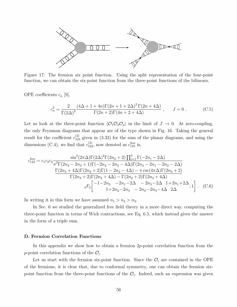
Figure 17: The fermion six point function. Using the split representation of the four-pointfunction, we can obtain the six-point function from the three-point functions of the bilinears.
OPE coefficients cn [9],
c2n =
2
Γ(2∆)2
(4∆ + 1 + 4n)Γ(2n+ 1 + 2∆)2 Γ(2n+ 4∆)
Γ(2n+ 2)Γ(4n+ 2 + 4∆), J = 0 . (C.5)
Let us look at the three-point function 〈O1O2O3〉 in the limit of J → 0. At zero-coupling,
the only Feynman diagrams that appear are of the type shown in Fig. 16. Taking the general
result for the coefficient c(2)123 given in (3.33) for the sum of the planar diagrams, and using the
dimensions (C.4), we find that c(2)123, now denoted as cfree
123 is,
cfree123 = c1c2c3
sin2(2π∆)Γ(2∆)2Γ(2n2 + 2)∏3
i=1 Γ(−2ni − 2∆)
π2Γ(2n2 − 2n3 + 1)Γ(−2n2 − 2n3 − 4∆)Γ(2n3 − 2n1 − 2n2 − 2∆)
Γ(2n3 + 4∆)Γ(2n2 + 2)Γ(1− 2n2 − 4∆)− π csc(4π∆)Γ(2n3 + 2)
Γ(2n3 + 2)Γ(2n2 + 4∆)− Γ(2n2 + 2)Γ(2n3 + 4∆)
4F3
[−1−2n3 −2n1−2∆ − 2n3−2∆ 1+2n1+2∆
1+2n2−2n3 − 2n2−2n3−4∆ 2∆; 1
]. (C.6)
In writing it in this form we have assumed n1 > n2 > n3.
In Sec. 6 we studied the generalized free field theory in a more direct way, computing the
three-point function in terms of Wick contractions, see Eq. 6.5, which instead gives the answer
in the form of a triple sum.
D. Fermion Correlation Functions
In this appendix we show how to obtain a fermion 2p-point correlation function from the
p-point correlation functions of the Oi.Let us start with the fermion six-point function. Since the Oi are contained in the OPE
of the fermions, it is clear that, due to conformal symmetry, one can obtain the fermion six-
point function from the three-point functions of the Oi. Indeed, such an expression was given
56
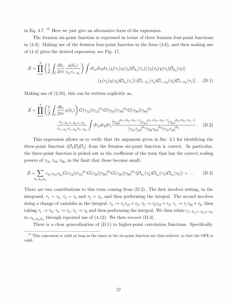
in Eq. 3.7. 15 Here we just give an alternative form of the expression.
The fermion six-point function is expressed in terms of three fermion four-point functions
in (4.3). Making use of the fermion four-point function in the form (4.6), and then making use
of (4.4) gives the desired expression, see Fig. 17,
S =3∏i=1
(1
2
∫C
dhi2πi
ρ(hi)
chic1−hi
)∫dτadτbdτc〈χ(τ1)χ(τ2)Oh1
(τa)〉〈χ(τ3)χ(τ4)Oh2(τb)〉
〈χ(τ5)χ(τ6)Oh3(τc)〉〈O1−h1
(τa)O1−h2(τb)O1−h3
(τc)〉 . (D.1)
Making use of (2.10), this can be written explicitly as,
S =3∏i=1
(1
2
∫C
dhi2πi
ρ(hi)
)G(τ12)|τ12|h1G(τ34)|τ34|h2G(τ56)|τ56|h3
c1−h1 1−h2 1−h3
c1−h1c1−h2
c1−h3
∫dτadτbdτc
|τab|h1+h2−h3−1|τac|h1+h3−h2−1|τbc|h2+h3−h1−1
|τa1τa2|h1|τb3τb4|h2|τc5τc6|h3. (D.2)
This expression allows us to verify that the argument given in Sec. 3.1 for identifying the
three-point function 〈O1O2O3〉 from the fermion six-point function is correct. In particular,
the three-point function is picked out as the coefficient of the term that has the correct scaling
powers of τ12, τ34, τ56, in the limit that these become small,
S =∑
h1,h2,h3
ch1ch2ch3G(τ12)|τ12|h1G(τ34)|τ34|h2G(τ56)|τ56|h3〈Oh1
(τ2)Oh2(τ4)Oh3
(τ6)〉+ . . . (D.3)
There are two contributions to this term coming from (D.2). The first involves setting, in the
integrand, τ1 = τ2, τ3 = τ4 and τ5 = τ6, and then performing the integral. The second involves
doing a change of variables in the integral, τa → τaτ12 + τ2, τb → τbτ34 + τ4, τc → τcτ56 + τ6, then
taking τ1 → τ2, τ3 → τ4, τ5 → τ6 and then performing the integral. We then relate c1−h1,1−h2,1−h3
to ch1,h2,h3through repeated use of (4.12). We then recover (D.3).
There is a clear generalization of (D.1) to higher-point correlation functions. Specifically,
15 This expression is valid as long as the times in the six-point function are time-ordered, so that the OPE isvalid.
57

Figure 18: There is an additional contribution to the eight-point function, involving four four-point functions meeting at a melon. This diagram is not planar, so it is difficult to draw. Wehave shown it for SYK with q = 6, unlike the other diagrams in the paper which are drawn forq = 4.
the leading order in 1/N fully connected piece of a 2p-point fermion correlation is given by,
1
N2p
∑i1,...,ip
〈χi1(τ1)χi2(τ2) · · ·χip(τ2p−1)χip(τ2p)〉 ⊃
p∏i=1
(1
2
∫C
dhi2πi
ρ(hi)
chic1−hi
)∫dτa1· · · dτap
p∏i=1
〈χ(τ2i−1)χ(τ2i)Ohi(τai)〉 〈O1−h1(τa1
) · · · O1−hp(τap)〉 .
E. Contact Diagrams
There is an additional contribution to the fermion eight-point function, shown in Fig. 18,
which has four ladders glued to a single melon,
Ec = (q − 1)(q − 2)(q − 3)J2
∫dτadτbG(τab)
q−44∏
i=1
F(τ2i−1, τ2i, τa, τb) . (E.1)
This gives rise to a contribution to the bilinear four-point function 〈O1(τ1) · · · O4(τ4)〉 that is,
C = c1c2c3c4(q − 1)(q − 2)(q − 3)bq∫dτadτb
|τab|24∏i=1
∣∣∣ τabτiaτib
∣∣∣hi . (E.2)
This diagram is novel, and unlike the other contributions to the four-point function studied in
the body of the paper, in the sense that it is not made up of fermion six-point functions glued
together.
For a 2p-point fermion correlation function, there will be an analogous, novel, contact dia-
gram, consisting of p ladders glued to a melon, as long q ≥ p. This term takes the form,
(q − 1)!
(q − p)!J2
∫dτadτbG(τab)
q−pp∏
i=1
F(τ2i−1, τ2i, τa, τb) , (E.3)
58
and gives a contribution to the p-point function 〈O1(τ1) · · · Op(τp)〉 that is,
c1 · · · cp(q − 1)!
(q − p)!bq∫dτadτb
|τab|2p∏i=1
∣∣∣ τabτiaτib
∣∣∣hi . (E.4)
These integrals can be rewritten in terms of conformal cross-ratios. For instance, for the four-
point function, we change variables to,
A =τa1τ23
τa2τ13
, B =τb2τ13
τb1τ23
, (E.5)
which gives,
C = c1c2c3c4(q−1)(q−2)(q−3) bq∣∣∣τ24
τ14
∣∣∣h12∣∣∣τ14
τ13
∣∣∣h34 1
|τ12|h1+h2|τ34|h3+h4
|x|h3+h4
|1− x|−h1+h2+h3IC , (E.6)
where,
IC =
∫dAdB
|1− AB|h1+h2+h3+h4−2
|A|h1|B|h2 |(1− A)(1−B)|h3|(A+ x− 1)(B + 1x−1
)|h4, (E.7)
where x is the cross-ratio of times. We will not proceed further with evaluating this integral,
however one could evaluate it using similar methods as those employed in the paper: considering
a restricted integration range and recognizing that portion of the integral as giving rise to a mul-
tivariable generalized hypergeometric function, finding all solutions to the differential equation
defining this function, and then writing the result for the integral as a linear combination of
solutions, and fixing the coefficients from different scaling limits.
F. Witten Diagrams
In this appendix we recall the evaluation of exchange and contact Witten diagrams [36–39].
Exchange diagram
Consider an s-channel exchange Witten diagram,Ws defined by (7.12) and shown in Fig. 15.
This involves external fields φi dual to operators Oi of dimension hi, and an exchanged φh, dual
to an operator Oh of dimension h. Making use of the split representation of the bulk propagator,
(7.10), we write this as,
Ws =
∫dhc2πi
ρw(h, hc)
∫∂AdS
dP0
∫AdS
dXdY Ghc(X,P0)G1−hc(Y, P0)
Gh1(X,P1)Gh2
(X,P2)Gh3(Y, P3)Gh4
(Y, P4) , (F.1)
59
where the integration contour is parallel to the imaginary axis 12− i∞<hc <
12
+ i∞, and we
defined,
ρw(h, hc) =2(hc − 1
2)2
(hc − h)(hc − 1 + h). (F.2)
We see that Ws involves a product of two three-point functions (7.4), integrated over P0. The
P0 integral, done in (A.12), gives a conformal block plus its shadow, leaving,
Ws =
∫dhc2πi
ρw(h, hc)ΛB∂(h1, h2, hc)ΛB∂(h3, h4, 1−hc)[β(hc, h34)Fhc1234(x) + β(1−hc, h12)F1−hc
1234 (x)].
We change integration variables hc → 1− hc for the second term, and use,
ΛB∂(h3, h4, hc)
ΛB∂(h3, h4, 1− hc)= −β(hc, h34)
Γ(hc)√π Γ(hc − 1
2), (F.3)
in order to write this as,
Ws =
∫dhc2πi
ρw(h, hc)ΛB∂(h1, h2, hc)ΛB∂(h3, h4, hc)Fhc1234(x) , (F.4)
where,
ρw(h, hc) = −2√π
Γ(hc − 12)
Γ(hc)ρw(h, hc) . (F.5)
If we wish, we can, for 0 < x < 1, close the contour to the right, writing the result as the
expected sum of single-trace and double-trace conformal blocks. For simplicity, we assume none
of the hi are equal and that h1 + h2 > 1/2 and h3 + h4 > 1/2. Then,
Ws = d(hi, h)Fh1234 +∞∑n=0
en(h1, h2, h3, h4, h)Fh1+h2+2n1234 +
∞∑n=0
en(h3, h4, h1, h2, h)Fh3+h4+2n1234 (F.6)
where the coefficient of the single-trace block is,
d(hi, h) = 2√π
Γ(h+ 12)
Γ(h)ΛB∂(h1, h2, h)ΛB∂(h3, h4, h) , (F.7)
while the coefficients of the double-trace blocks are,
en(h1, h2, h3, h4, h) = −ρw(h, h1+h2+2n)ΛB∂(h3, h4, h1+h2+2n) Res ΛB∂(h1, h2, hc)∣∣∣hc=h1+h2+2n
60
where,
Res ΛB∂(h1, h2, hc)∣∣∣hc=h1+h2+2n
= −2(−1)n
n!
Γ(h1 + h2 + n− 12)Γ(h1 + n)Γ(h2 + n)
16πΓ(h1 + 12)Γ(h2 + 1
2)Γ(h1 + h2 + 2n+ 1
2).
Contact diagram
One can evaluate a contact Witten diagram using similar methods. Consider the contact
diagram arising from the interaction, φ1φ2φ3φ4. We need to evaluate,
Wc =
∫AdS
dX Gh1(X,P1)Gh2
(X,P2)Gh3(X,P3)Gh4
(X,P4) . (F.8)
We may trivially rewrite this as,
Wc =
∫AdS
dXdY Gh1(X,P1)Gh2
(X,P2)δ(X − Y )Gh3(Y, P3)Gh4
(Y, P4) , (F.9)
and use the split-representation of the delta function [30],
δ(X − Y ) =
∫dhc2πi
ρc(hc)
∫∂AdS
dP0 Ghc(X,P0)G1−hc(Y, P0) , (F.10)
where the contour is as before, and,
ρc(hc) = −2(hc −1
2)2 . (F.11)
Following the same steps as in the calculation of the exchange Wittten diagram gives for the
contact Witten diagram,
Wc =
∫dhc2πi
ρc(hc)ΛB∂(h1, h2, hc)ΛB∂(h3, h4, hc)Fhc1234(x) , (F.12)
where,
ρc(hc) = −2√π
Γ(hc − 12)
Γ(hc)ρc(hc) . (F.13)
If we wish, we can, for 0 < x < 1, close the contour to the right and write Wc as a sum of
double-trace conformal blocks.
A general quartic interaction in the bulk will involve derivatives. For any specific set of
derivatives it straightforward to write the contact Witten diagram as a sum of conformal blocks,
as in the above case without derivatives, but it is difficult to write a general expression.
61
G. An AdS2 Brane in AdS3
The SYK model contains a tower of primary O(N) invariant bilinears, On, with dimensions
hn. By the AdS/CFT dictionary, these are dual to a tower of massive fields φn with masses,
m2n = hn(hn − 1) . (G.1)
For SYK at large q, the dimensions are, to leading order in 1/q, given by hn = 2n+1. Therefore,
for large n, the masses are approximates mn ≈ 2n+ 1. A natural way to approximately produce
a spectrum of this type is to view it as arising from a Kaluza-Klein tower of a single scalar field
in AdS2×S1. 16 To account for the bulk cubic couplings λnmkφnφmφk, it is natural to introduce
a cubic interaction φ3 in the AdS2×S1 space. One can then trivially compute the resulting cubic
couplings: they are given by overlaps of the wavefunctions eimθ along the S1. These couplings
are, however, clearly a poor approximation to the true λnmk, given in (6.29). For instance, these
are of order-one, whereas the actual λnmk grow exponentially as n,m, k uniformly get large.
The spectrum of the scalar in AdS2×S1 is only approximately that of large-q SYK for n� 1.
In this appendix we will show that placing an AdS2 brane inside of AdS3, and considering a
scalar in the AdS3 spacetime, will exactly reproduce the large q SYK spectrum. However, the
cubic couplings will still be completely off. This illustrates, perhaps unsurprisingly, that the
spectrum is not by itself a strong enough clue as to the nature of the bulk theory.
We write AdS3 in coordinates,
ds2 = dr2 + cosh2 r ds22 , (G.2)
where ds22 is the metric on AdS2. Which coordinates one picks on the AdS2 will not be relevant
for us; a simple choice is global coordinates,
ds22 =
1
cos2 ρ
(−dt2 + dρ2
). (G.3)
The interpretation of (G.2) is that at each r there is an AdS2 space with radius cosh r. The
range of r is from −∞ to ∞.
We place a brane at some constant r, which without loss of generality, we take to be at
r = 0. The tension of the brane is tuned so that it is static; for a general discussion, see [41].
16We thank N. Nekrasov for discussions on this.See [40] for work in a similar direction.
62

The wave equation for a scalar in AdS3,(�−m2
)φ = 0, in terms of coordinates (G.2) is,
1
cosh2 r∂r(cosh2 r ∂rφ
)+
1
cosh2 r�2φ = m2φ , (G.4)
where �2 is the AdS2 Laplacian. Letting the solution be of the form,
φ(r, ρ, t) = f(r)ψ(ρ, t) , f(r) =u(r)
cosh r, (G.5)
and letting m22 denote the eigenvalue of the AdS2 Laplacian, �2 ψ(ρ, t) = m2
2 ψ(ρ, t), we get that
the radial wavefunction satisfies,
− 1
2u′′(r)− m2
2
2 cosh2 ru(r) = −(m2 + 1)
2u(r) . (G.6)
This is of the form of a Schrodinger equation for a particle of energy −(m2 + 1)/2 in a potential
−m22/(2 cosh2 r). Note that the mass m is fixed: this is the mass of the scalar in AdS3, which
we choose at the beginning. On the other hand, m2 is arbitrary and will only be constrained by
quantization requirements. In particular, in order for −(m2 + 1)/2 to be an eigenenergy of the
potential, the values m22 can not be arbitrary. This is a bit different from the scenario in which
one compactifies along a compact manifold.
In fact, this potential is the Poschl-Teller potential. Letting,
m22 = n(n+ 1) , µ2 = m2 + 1 , (G.7)
where n is a positive integer, the eigenenergies are µ = 1, 2, . . . , n. The eigenfunctions are the
associated Legendre functions, u(r) = P µλ (tanh(r)).
We will choose the AdS3 scalar to be massless, m = 0. Then, from the point of view of the
AdS2 brane, a massless particle in AdS3 looks like a tower of particles with masses m22 = n(n+1).
This reproduces the large q SYK spectrum, up to the fact that we should keep only odd n.
This can be achieved through an appropriate choice of boundary conditions, as the Legendre
polynomials P 1n (tanh(r)) are odd under r → −r for even n, and even for odd n.
Let us now compute the cubic couplings. In the AdS3 space we take the action,
S =
∫dtdρdr
√−g(φ�φ+ λφ3
)(G.8)
and insert
φ =∞∑n=1
fn(r)ψn(ρ, t) , fn(r) =1
cosh rP 1n (tanh(r)) . (G.9)
63
We rewrite the action as,
S =
∫dρdt√−g2
∑n,m
(∫fn(r)fm(r)
)ψn(ρ, t)
(�2 − n(n+ 1)
)ψm(ρ, t)
+
∫dρdt√−g2
∑n,m,k
(∫dr cosh2 rfn(r)fm(r)fk(r)
)ψn(ρ, t)ψm(ρ, t)ψk(ρ, t) , (G.10)
where g2 denotes the determinant of the AdS2 metric. Rescaling the fields,
ψn = Nn ψn , N2nδnm =
∫dr fn(r)fm(r) , N2
n =2n(1 + n)
1 + 2n, (G.11)
we have,
S =
∫dρdt√−g2
[∑n,m
ψn
(�2 − n(n+ 1)
)ψn + λnmkψnψmψk
](G.12)
where,
λnmk =λ
NnNmNk
∫dr cosh2 r fn(r)fm(r)fk(r) . (G.13)
Evaluating λnnn, the growth with n is slow, and inconsistent with the required couplings of the
bulk dual of SYK, (6.29).
References
[1] N. Beisert et al., “Review of AdS/CFT Integrability: An Overview,” Lett. Math. Phys. 99
(2012) 3–32, arXiv:1012.3982 [hep-th].
[2] A. Z. Patashinskii and V. L. Pokrovskii, “Second Order Phase Transitions in a Bose Fluid,”
JETP 19 (1964) 677.
[3] S. Sachdev and J. Ye, “Gapless spin-fluid ground state in a random quantum heisen-
berg magnet,” Phys. Rev. Lett. 70 (May, 1993) 3339–3342. http://link.aps.org/doi/
10.1103/PhysRevLett.70.3339.
[4] R. Gurau, “Colored Group Field Theory,” Commun. Math. Phys. 304 (2011) 69–93,
arXiv:0907.2582 [hep-th].
[5] A. Kitaev, “A simple model of quantum holography,” KITP strings seminar and Entan-
glement 2015 program (Feb. 12, April 7, and May 27, 2015) . http://online.kitp.ucsb.
edu/online/entangled15/.
64
[6] D. J. Gross and V. Rosenhaus, “The Bulk Dual of SYK: Cubic Couplings,” JHEP 05 (2017)
092, arXiv:1702.08016 [hep-th].
[7] J. Polchinski and V. Rosenhaus, “The Spectrum in the Sachdev-Ye-Kitaev Model,” JHEP
04 (2016) 001, arXiv:1601.06768 [hep-th].
[8] J. Maldacena and D. Stanford, “Comments on the Sachdev-Ye-Kitaev model,”
arXiv:1604.07818 [hep-th].
[9] D. J. Gross and V. Rosenhaus, “A line of CFTs: from generalized free fields to SYK,” JHEP
07 (2017) 086, arXiv:1706.07015 [hep-th].
[10] A. Gadde, “In search of conformal theories,” arXiv:1702.07362 [hep-th].
[11] D. J. Gross and V. Rosenhaus, “A Generalization of Sachdev-Ye-Kitaev,” JHEP 02 (2017)
093, arXiv:1610.01569 [hep-th].
[12] E. Witten, “An SYK-Like Model Without Disorder,” arXiv:1610.09758 [hep-th].
[13] Y. Gu, X.-L. Qi, and D. Stanford, “Local criticality, diffusion and chaos in generalized
Sachdev-Ye-Kitaev models,” JHEP 05 (2017) 125, arXiv:1609.07832.
[14] W. Fu, D. Gaiotto, J. Maldacena, and S. Sachdev, “Supersymmetric Sachdev-Ye-Kitaev
models,” Phys. Rev. D95 no. 2, (2017) 026009, arXiv:1610.08917 [hep-th]. [Addendum:
Phys. Rev.D95,no.6,069904(2017)].
[15] R. A. Davison, W. Fu, A. Georges, Y. Gu, K. Jensen, and S. Sachdev, “Thermoelectric trans-
port in disordered metals without quasiparticles: The Sachdev-Ye-Kitaev models and holog-
raphy,” Phys. Rev. B95 no. 15, (2017) 155131, arXiv:1612.00849 [cond-mat.str-el].
[16] J. Murugan, D. Stanford, and E. Witten, “More on Supersymmetric and 2d Analogs of the
SYK Model,” JHEP 08 (2017) 146, arXiv:1706.05362 [hep-th].
[17] X.-Y. Song, C.-M. Jian, and L. Balents, “A strongly correlated metal built from Sachdev-
Ye-Kitaev models,” arXiv:1705.00117 [cond-mat.str-el].
[18] V. Bonzom, R. Gurau, A. Riello, and V. Rivasseau, “Critical behavior of colored ten-
sor models in the large N limit,” Nucl. Phys. B853 (2011) 174–195, arXiv:1105.3122
[hep-th].
[19] I. R. Klebanov and G. Tarnopolsky, “Uncolored Random Tensors, Melon Diagrams, and
the SYK Models,” arXiv:1611.08915 [hep-th].
65

[20] I. R. Klebanov and G. Tarnopolsky, “On Large N Limit of Symmetric Traceless Tensor
Models,” JHEP 10 (2017) 037, arXiv:1706.00839 [hep-th].
[21] K. Bulycheva, I. R. Klebanov, A. Milekhin, and G. Tarnopolsky, “Spectra of Operators in
Large N Tensor Models,” arXiv:1707.09347 [hep-th].
[22] S. Choudhury, A. Dey, I. Halder, L. Janagal, S. Minwalla, and R. Poojary, “Notes on
Melonic O(N)q−1 Tensor Models,” arXiv:1707.09352 [hep-th].
[23] I. Heemskerk, J. Penedones, J. Polchinski, and J. Sully, “Holography from Conformal Field
Theory,” JHEP 10 (2009) 079, arXiv:0907.0151 [hep-th].
[24] M. Hogervorst and B. C. van Rees, “Crossing Symmetry in Alpha Space,”
arXiv:1702.08471 [hep-th].
[25] M. Cho, S. Collier, and X. Yin, “Recursive Representations of Arbitrary Virasoro Conformal
Blocks,” arXiv:1703.09805 [hep-th].
[26] C. Sleight and M. Taronna, “Higher Spin Interactions from Conformal Field Theory: The
Complete Cubic Couplings,” Phys. Rev. Lett. 116 no. 18, (2016) 181602, arXiv:1603.00022
[hep-th].
[27] X. Bekaert, J. Erdmenger, D. Ponomarev, and C. Sleight, “Towards holographic higher-
spin interactions: Four-point functions and higher-spin exchange,” JHEP 03 (2015) 170,
arXiv:1412.0016 [hep-th].
[28] X. Bekaert, J. Erdmenger, D. Ponomarev, and C. Sleight, “Quartic AdS Interac-
tions in Higher-Spin Gravity from Conformal Field Theory,” JHEP 11 (2015) 149,
arXiv:1508.04292 [hep-th].
[29] C. Sleight and M. Taronna, “Spinning Witten Diagrams,” JHEP 06 (2017) 100,
arXiv:1702.08619 [hep-th].
[30] J. Penedones, “Writing CFT correlation functions as AdS scattering amplitudes,” JHEP
03 (2011) 025, arXiv:1011.1485 [hep-th].
[31] F. A. Dolan and H. Osborn, “Conformal four point functions and the operator product
expansion,” Nucl. Phys. B599 (2001) 459–496, arXiv:hep-th/0011040 [hep-th].
[32] S. Ferrara, A. F. Grillo, G. Parisi, and R. Gatto, “The shadow operator formalism for confor-
mal algebra. vacuum expectation values and operator products,” Lettere al Nuovo Cimento
(1971-1985) 4 no. 4, (May, 1972) 115–120. https://doi.org/10.1007/BF02907130.
66

[33] D. Simmons-Duffin, “Projectors, Shadows, and Conformal Blocks,” JHEP 04 (2014) 146,
arXiv:1204.3894 [hep-th].
[34] K. Bulycheva, “A note on the SYK model with complex fermions,” arXiv:1706.07411
[hep-th].
[35] G. Mack, “D-independent representation of Conformal Field Theories in D dimensions via
transformation to auxiliary Dual Resonance Models. Scalar amplitudes,” arXiv:0907.2407
[hep-th].
[36] H. Liu, “Scattering in anti-de Sitter space and operator product expansion,” Phys. Rev.
D60 (1999) 106005, arXiv:hep-th/9811152 [hep-th].
[37] S. El-Showk and K. Papadodimas, “Emergent Spacetime and Holographic CFTs,” JHEP
10 (2012) 106, arXiv:1101.4163 [hep-th].
[38] M. S. Costa, V. Gonalves, and J. Penedones, “Spinning AdS Propagators,” JHEP 09 (2014)
064, arXiv:1404.5625 [hep-th].
[39] E. Hijano, P. Kraus, E. Perlmutter, and R. Snively, “Witten Diagrams Revisited: The AdS
Geometry of Conformal Blocks,” JHEP 01 (2016) 146, arXiv:1508.00501 [hep-th].
[40] S. R. Das, A. Jevicki, and K. Suzuki, “Three Dimensional View of the SYK/AdS Duality,”
JHEP 09 (2017) 017, arXiv:1704.07208 [hep-th].
[41] A. Karch and L. Randall, “Locally localized gravity,” JHEP 05 (2001) 008,
arXiv:hep-th/0011156 [hep-th].
67