all together now: the impact of a multifaceted approach to

All together now: the impact of a multifacetedapproach to poverty alleviation∗

Vilas J. Gobin† Paulo Santos‡

This version: December 2015

Abstract

We examine the impact of the Rural Entrepreneur Access Program(REAP), an example of an approach that combines multiple inter-ventions with the aim of overcoming the constraints facing the ultra-poor. This program was implemented in an extreme setting (arid areasof northern Kenya) and emphasizes cash transfers (rather than assettransfers) to ultra-poor women, in addition to business skills training,business mentoring and savings trainings. Due to over-recruitment,the program was rolled-out in three rounds, with allocation to eachround being randomly determined through a public lottery. In theshort-run we find that the program has a positive and significant im-pact on income, savings and asset accumulation and food security.

∗We thank Russell Toth, Gaurav Datt, Hee-Seung Yang, Asadul Islam and AndreasLeibbrandt for comments on earlier drafts of this paper. The data used in this study weresupplied by The BOMA Project. We thank staff of The BOMA Project especially Kath-leen Colson, Ahmed Omar, Meshack Omarre, Fredrick Learapo, Sabdio Doti, BernadetteNjoroge, Nate Barker, and Alex Villec for their assistance in data collection as well asin facilitating the first author’s stay in Kenya. All analyses, interpretations or conclu-sions based on these data are solely that of the authors. The BOMA Project disclaimsresponsibility for any such analyses, interpretations or conclusions.†PhD Student, Economics, Monash University, Melbourne, Australia. Corresponding

author (e-mail: [email protected])‡Senior Lecturer, Economics, Monash University, Melbourne, Australia.

1

1 Introduction

Microenterprises are the source of employment for more than half of the

labor force in developing countries (de Mel, S., D., & Woodruff, 2008; Gin-

dling & Newhouse, 2014), and are seen as engines of economic development

by raising income of managers, creating a demand for labor (earning higher

wages), and increasing market competition (that generates lower prices to

consumers) (Bank, 2012; Bruhn, 2011). Despite these benefits, it has been

realized that the world’s poorest are often prevented from establishing such

businesses or from participating in many popular approaches aimed at stim-

ulating microenterprise formation.

For example, until very recently microfinance was advocated as a way to

overcome financial market imperfections which limited the capacity of the

poor to invest in profitable projects (Jolis & Yunus, 2003). Recent evidence

points to the limited impact of microfinance on poverty alleviation suggest-

ing that alleviating credit constraints alone is not sufficient to reduce poverty

through microenterprises (e.g. Angelucci, Karlan, & Zinman, 2014; Baner-

jee, Duflo, Glennerster, & Kinnan, 2013; Banerjee, Karlan, & Zinman, 2015;

Karlan & Zinman, 2010). This has prompted a shift in attention to other

possible constraints, particularly entrepreneurial skills, knowledge and hu-

man capital. But the conclusions of evaluations of interventions designed to

overcome these constraints have been mixed (e.g. Bruhn, Karlan, & Schoar,

2013; Drexler, Fischer, & Schoar, 2014; Valdivia, 2015).

The limited impact of this “one-constraint-at-a-time” approach, particu-

larly among the ultra-poor, suggested the need for interventions that simulta-

neously address the overlapping set of constraints and provide the ultra-poor

with a localized “big push” to graduate from poverty. One influential ap-

proach, pioneered by BRAC, is the Challenging the Frontiers of Poverty Re-

duction - Targeting the Ultra-Poor (CFPR/TUP), structured as a poverty

graduation program: during a limited period (two years), its participants

would benefit from a set of interventions (savings services, skills training,

2

and a physical asset transfer, together with regular follow-up visits and con-

sumption support) with the expectation that, at the end of that period, par-

ticipants would be able to participate in microfinance (Goldberg & Salomon,

2011; Matin, Sulaiman, & Rabbani, 2008).

There is limited understanding of the impact of this type of intervention

on poverty alleviation given its relative novelty but the existing studies find

that it does lead to sustained improvements in household welfare as a result

of increased incomes from self-employment activities. A randomized evalu-

ation of CFPR/TUP across 1409 communities in Bangladesh finds that the

program enabled ultra-poor women to engage in microentrepreneurial activ-

ities resulting in a significant increase in earnings, which persists up to two

years after participants graduate from the program (Bandiera et al., 2013).

Evidence also comes from some of the 20 countries where this approach

has been replicated or adapted. In a recent multi-site randomized evalua-

tion across six of these countries, Banerjee, Duflo, et al. (2015) find similar

impacts to those reported for Bangladesh: consumption, productive assets,

income and revenue are higher in the treatment group at the conclusion of

the program and remain higher one year after graduation. However, these

impacts are found to be weaker in two study sites (Honduras and Peru),

naturally raising questions about the external validity of the results.

Concerns about external validity are also present in another study in

Andhra Pradesh, India, where Bauchet, Morduch, and Ravi (2015) evaluate

a similar intervention and finds no net impact on consumption, income or

asset accumulation. The authors suggest that the muted impacts could be

explained by a strong labor market which sharply increased the wages for

unskilled labor, highlighting the need to consider factors such as the eco-

nomic environment in which households make decisions when addressing the

external validity of these evaluations.

This paper examines the impact of the Rural Entrepreneur Access Project

(REAP), a variation of the CFPR/TUP graduation approach, implemented

3

in northern Kenya, a region where more than 80% of the population is esti-

mated to be living below the national poverty line (of Statistics & for Inter-

national Development, 2013). The Rural Entrepreneur Access Project com-

prises of an initial package of interventions, including business skills training,

cash transfers to set up a microenterprise and business mentoring which were

followed, six months later, by a focus on the importance of savings (training

and introduction to savings groups). 1 This sequence of interventions is tar-

geted at ultra-poor women and is designed to enable them to gain the assets

and skills necessary to graduate from poverty, a motivation that is similar to

the one behind the CFPR/TUP (MacMillan, 2013).

There are however important differences, chief among them being the fact

that women are provided with a cash transfer instead of an asset transfer, as

in other poverty graduation programs studied to date (e.g. Bandiera et al.,

2013; Banerjee, Duflo, et al., 2015; Bauchet et al., 2015). Cash transfers are

arguably more attractive in that they allow the participants more freedom

in their choice of enterprise and are potentially less costly to implement. 2

The program also differs in two other important ways: there is no provision

of consumption support (which could potentially aggravate the risk of the

cash transfer being used for consumption) and, finally, beneficiaries are re-

quired to work as a group in running their enterprise. The primary objective

of this paper is to determine if jointly relaxing financial and human cap-

ital constraints results in poverty alleviation through microentrepreneurial

activities.

The remainder of the paper proceeds as follows. In section 2 we provide

a detailed description of REAP before presenting, in section 3, the identifica-

1The program is implemented through a NGO, The BOMA Project. See http://

bomaproject.org/the-rural-entrepreneur-access-project/ for a complete descrip-tion of REAP.

2The preference for an asset transfer is usually justified by fears that cash transferscould be immediately spent on consumption instead of invested in an enterprise. SeeAnnan, Blattman, Green, Jamison, and Lehmann (2015) for empirical evidence againstsuch belief.

4

tion strategy and the data used in this paper. We are able to take advantage

of randomized roll-out of the program, which resulted from over-recruitment

during the participant selection stage of the program, to obtain unbiased esti-

mates of the program’s impact on household welfare. Section 3 also includes

tests of the assumptions underlying the identification strategy and a discus-

sion of spillover and anticipation effects. The main results are presented in

section 4. We find that, in the short-run, this program has a positive and sta-

tistically significant impact on income, savings and asset accumulation (both

consumer durables and productive assets), and food security (as measured

by the number of nights children went to bed hungry). However, we do not

find an impact on consumption. We conclude in section 5.

2 Overview of the intervention

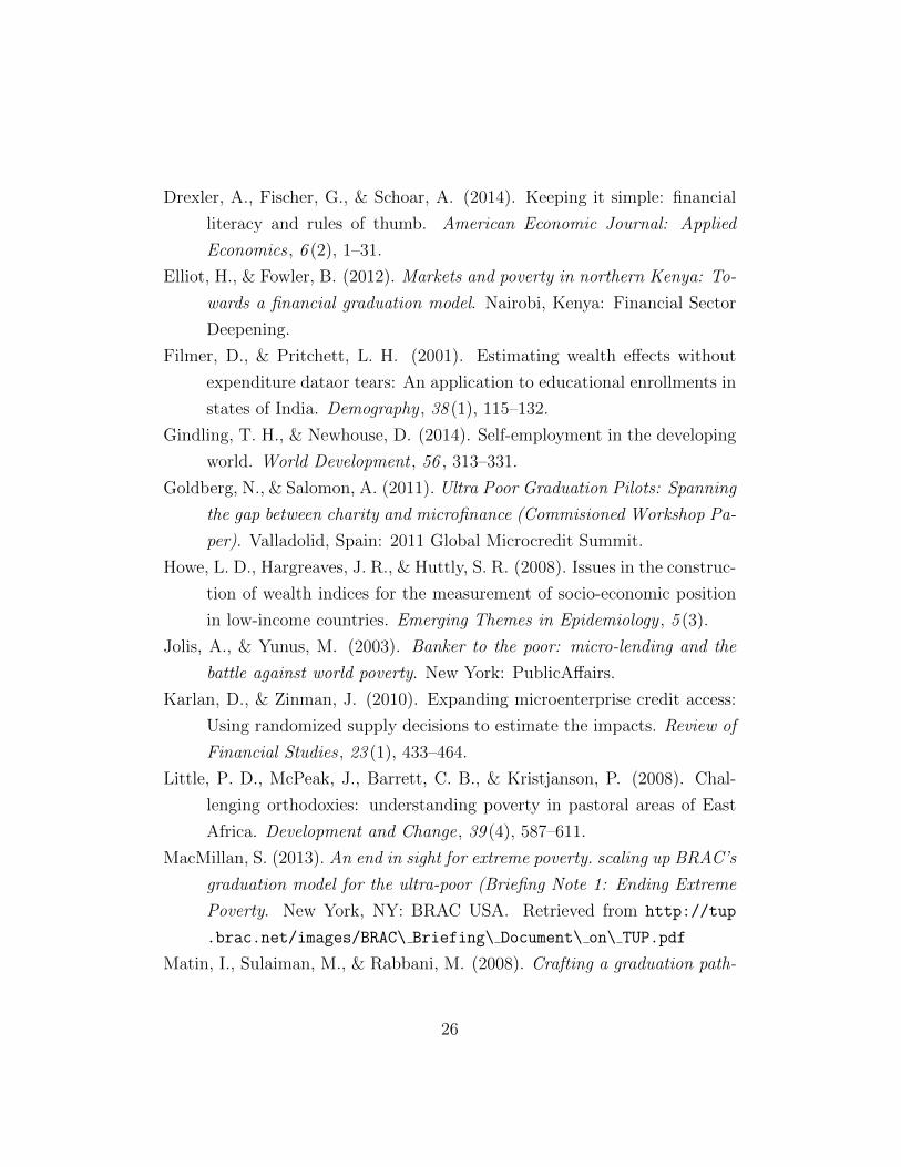
The Rural Entrepreneur Access Project was implemented in 14 locations in

the southern and central parts of Marsabit County, in the Arid and Semi-Arid

Lands (ASALs) of northern Kenya (see Figure 1), a region where more than

80% of the population are estimated to live below the national poverty line (of

Statistics & for International Development, 2013). 3 The main livelihood op-

tion in these locations is pastoralism, with livestock serving both as a source

of income and food for herders and their families. Pastoralism, however, is

highly susceptible to weather and other shocks, and repeated droughts fre-

quently have devastating impacts on households’ livelihoods (Silvestri, Bryan,

Ringler, Herrero, & Okoba, 2012), resulting in many households no longer

being able to meet their basic needs due to the loss of herds. Such households

are forced into begging, unskilled wage labor, different forms of petty trade,

3In 2005/06, the poverty line was estimated at Ksh 1,562 (PPP USD 77.07 at 2014prices) per adult equivalent per month for rural households (of Statistics, 2007). In 2009it was estimated that nationally, 45.2% of the population lived below the poverty line (ofStatistics & for International Development, 2013).

5

and become reliant on food aid to meet their dietary needs. 4

Opportunities to engage in non-pastoral activities are further restricted

by the fact that communities in this region tend to be excluded from national

development processes, have low population densities (<5/km2), have lim-

ited access to markets or other infrastructure, and face financial and human

capital constraints (Elliot & Fowler, 2012). By targeting the poorest women

in these communities, REAP aims to provide the most vulnerable households

with a pathway out of poverty by alleviating the financial and human capital

constraints that they face.

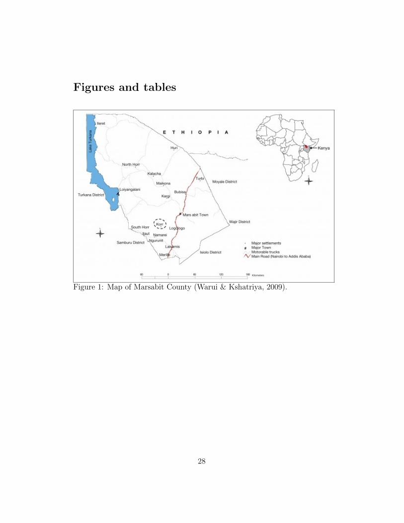
2.1 Structure and timing of the program

The main aim of REAP is to graduate ultra-poor women from poverty,

through a set of interventions that include the development of business plans

and mentoring, grants and access to saving mechanisms. The sequence of

these interventions is presented in Figure 2, and each intervention is briefly

described below.

Participant Selection. Program eligibility is determined by local committees,

formed specifically for targeting. 5 These committees were asked to identify

women who were among the poorest of the poor in the community, with no

other sources of income besides the business being formed, and who were also

considered to be responsible and entrepreneurially minded, and were willing

to run a business with two other women. 6 Trained business mentors ensured

4Little, McPeak, Barrett, and Kristjanson (2008) examine different proxies for povertyand welfare in northern Kenya. They identify poverty as being most prevalent amongsedentary households that are no longer directly involved in pastoral production or are inthe process of exiting pastoralism. They have little or no livestock and tend to be involvedin unskilled wage labour and petty trade.

5The committees genrally comprise 10 persons, with equal representation of clans andethnic groups in the community, and with at least half of them being women.

6In addition, and recognizing the importance of inter-ethnic rivalries in northern Kenya,selection committees were asked to select participants in order to lead to an equal rep-resentation from various clans and ethnic groups and appropriate representation of per-sons from the town centre and more distant villages. Finally, immediate relatives of any

6

that the local committees followed these criteria when selecting participants. 7

Once the participants were selected and accepted the invitation to participate

in REAP, the business mentor proceeded to form business groups of three

women.

Business Planning and Business Skills Training. In the month leading up

to program enrollment, the business mentors met with beneficiaries to assist

with the development of a business proposal. The mentor was expected to get

a better understanding of the group members’ abilities and previous business

experience before going through the basics of setting up a business with the

group. 8 On the day of program enrolment, all participants were required

to attend a short business skills training session, delivered by mentors under

the supervision of REAP field officers. 9

First Grant and Business Mentoring. At the end of the business skills train-

ing session participants were provided with a cash grant of USD 100 (PPP

USD 237.97 at 2014 prices) to be used to establish their business, an amount

which is equivalent to approximately 7.5 months of expenditure per capita. 10

Once the groups received their grants they were free to invest the money, in-

cluding by making changes in their initial business proposal.

BOMA Project staff were considered ineligible. More recently, participant selection pro-cedures included a Participatory Wealth Ranking to identify the poorest, followed by ashort interview, used to confirm eligibility.

7Mentors are employed at the location level. Each location comprises many sub-locations which are formed by smaller villages, known as manyattas.

8This early training session included: understanding the needs and size of the market,identification of the type of business that will be established and its location, identifica-tion of suppliers, decisions regarding how to spend the initial grant (and other inputs),allocation of responsibilities among group members, and, finally, decisions regarding howprofits are to be used.

9Which covered the following topics: what is a business; how to make a profit; what tosell (or produce); how to attract customers; management of the business; record keeping;and the value of savings.

10All monetary values reported in the paper are in PPP terms at 2014 prices. We usethe following PPP exchange rates to convert Kenya Shillings to USD PPP: 36.83 (2012),38.38 (2013), 40.35 (2014). These values are then converted to 2014 prices by multiplyingthe ratio of the 2014 US Consumer Price Index (CPI) to the US CPI for the relevant year.

7

The distribution of the initial grants was followed by a period during

which a mentor regularly met with the business group (at least once a month)

to monitor its progress and offer advice and training. The role of the mentor

was to help in the start-up of the business, through the provision of informa-

tion (such as where to source goods and market conditions). Additionally, it

was expected that, by providing ongoing training and support, the mentor

would help the group with record keeping and, if needed, in managing con-

flicts within the group. Mentoring would last until groups formally exit the

program, two years after its start.

Second Grant, Savings Training and Savings Group Formation. Six months

after the start of the business, groups were eligible for a follow up grant of

USD 50 (PPP USD 118.98) conditional on meeting the following criteria:

two or more original members remained involved in the business; members

held business assets collectively; and the business value (defined as the sum

of cash on hand, business savings and credit outstanding, and business stock

and assets) was equal to or greater than the value of the initial grant. Partici-

pants were also required to participate in a short training session on savings,

designed to provide a basic understanding of the formation and operation

of savings groups including their rules, record-keeping, and issuing of loans.

These conditions were known by participants since the start of the program.

After the savings training and the second grant distribution, participants

were encouraged to form a savings group (SG) or join existing ones. The

decision to join a group was both non-compulsory and individual (i.e., it

was not a business group decision). The savings group model introduced

to participants during the training most closely resembled Village Savings

and Loans Associations (VSLA), also known as Accumulating Savings and

Credit Associations (ASCAs), described in Allen (2006). The groups are

self-managed and allow members to save money and access loans which are

paid back with interest.

8

3 Research design

3.1 Randomization of program assignment

In November 2012, the local selection committees across 14 locations in north-

ern Kenya, identified 1755 women as being eligible for REAP. Due to lack

of capacity to simultaneously enroll all participants, it was decided to split

the eligible women into three groups to be successively enrolled over the

next three funding cycles (March/April 2013, September/October 2013 or

March/April 2014, hereafter groups A, B and C, respectively). 11 Assign-

ment to each cycle was done randomly, through a public lottery that took

place in each of the 14 locations from which participants had been recruited,

with one-third of the women enrolled in each funding cycle. 12 A public lot-

tery was used to ensure that the allocation to funding cycle was transparent

and fair, and seen as such. The random assignment of the beneficiaries to

each cycle, if not defied, should lead to balanced groups, statistically identi-

cal in all observable (and, by assumption, unobservable) characteristics. All

eligible women were interviewed at baseline (November 2012) and at two

follow-up surveys, conducted at six month intervals and timed to coincide

with the beginning of each new funding cycle. 13

None of the eligible participants declined to participate in the program, or

was allowed to participate outside of the group to which they were randomly

allocated. Survey attrition is very low in both follow-up rounds of survey.

Less than 2% of women could not be reached for a follow-up interview in

11As a result, sample size was determined by the capacity of the program to reachparticipants. We conduct ex post power calculations to determine if there is sufficientpower, given the predetermined sample size, to reliably estimate program impacts, andfind that in most cases the minimum detectable effect size is as low as 15%. Thesecalculations are available from the authors upon request.

12Initially 1755 women were selected, but 3 women were subsequently disqualified lead-ing to 585 women being assigned to the first and second cycles and 582 women beingassigned to the final funding cycle.

13Figure A1, in Appendix A, presents a timeline and sequence of activities for partici-pants in the three funding cycles, including the timing of the surveys.

9

either the midline or endline surveys (see Table 1).

Together, the sequential rollout of the program, the randomized allocation

to each cycle, the perfect compliance of observations to treatment and control

groups, and the extremely low attrition rate, allow us to disentangle some of

the program impacts in a relatively straightforward way.

3.2 Checking the integrity of randomized design

We test the assumption that baseline characteristics are uncorrelated with

treatment status by comparing the distribution of the baseline characteristics

of participants. We make several comparisons that take into account the

changing composition of the treatment and control groups as the program is

progressively rolled-out. The results are presented in Table 2.

In panel A, we present summary statistics (mean and standard devia-

tions) of variables that may be impacted by the program (expenditure, in-

come, savings, asset ownership) or that may mediate its impact (household

size, previous business experience, education). The baseline characteristics

of the participants (and their households) are similar to those of other ultra-

poor households in other regions of northern Kenya, which suggests that the

findings of this study may be generalizable to ultra-poor pastoralist women

across northern Kenya (Merttens et al., 2013). Average monthly expenditure

per capita is approximately PPP USD 33.96, which is well below the poverty

line. Approximately 70% of this expenditure is on food. Households are rel-

atively large and have approximately 3.8 children on average, with less than

50% of children enrolled in school. Many households are food insecure, with

children going to bed hungry at least 2 times a month. Women also report

owning very little livestock: less than one Tropical Livestock Unit (TLU)

per capita, well below the self-sufficiency threshold for mobile pastoralists in

East African ASALs (McPeak & Barrett, 2001). 14 However, more than half

14Tropical Livestock Unit (TLU) is a standardized unit, designed to measure the size ofa mixed livestock herd: 1 TLU is equivalent to 1 head of cattle, 0.7 camels, 10 sheep/goats,

10

of the participants report having some form of business experience, typically

petty trade or the selling of livestock and livestock products.

In panel B, we present the t-tests of the null hypothesis of equality of

means at baseline. These results indicate that randomization was successful

in creating groups of individuals that are observationally identical, and in

only one case can we reject the null hypothesis at the conventional 5% level.

This conclusion is reinforced by the results of a F -test of the joint effect of

these variables on treatment status, reported in panel C.

3.3 Spillover effects and program anticipation

Given the geographical proximity of individuals in the treatment and con-

trol groups, it is possible that control households use and benefit from the

products and services offered by the businesses established by the treated

households. Given that more than 95% of the businesses that are established

by the treated individuals are in petty trade (primarily of food items), the

main benefit might be increased competition among businesses, with a con-

sequent reduction in market prices. Although this reduction is not expected

to be substantial given the large number of pre-existing businesses in each

location, we are able to control for this general equilibrium effect through

the inclusion of the number of pre-existing businesses as a control variable

when estimating the effect of the program. 15

Another potential source of spillover effects might be easier access to

loans. Although only REAP participants can actively participate in all SG

activities, loans can be (and typically, are) extended to other members of

the community, so that they can deal with shocks and emergencies (usually,

health, or school and food related expenditures). We capture information on

borrowing from REAP SGs for all women, and therefore can control for this

or 2 donkeys.15Overall, there were 1932 businesses before the program. The program funded 195

businesses (approximately 10% of the pre-existing number) in each funding cycle. SeeTable B1, in Appendix B, for further details.

11

effect when estimating the impact of the program.

Finally, bias could potentially arise from participants changing their be-

havior in anticipation of receiving the program. If true, then we would expect

that the effect of such changes would differ between individuals that enroll

in the program in the second and third funding cycles, given that one group

would anticipate receiving funding six months sooner than the other. 16 If

this intuition is correct, these differences would then be captured during

the midline survey (when group B is expected to immediately receive the

first grant while group C is still six months away from participating in the

program). As shown in Table 3, we find no evidence of program anticipa-

tion effects. 17 We also collected information on income earned from other

businesses (besides REAP businesses) in all rounds of data collection, which

allows us to examine if anticipation of the program led to investment in a

business that did not exist at baseline. We find no evidence of statistically

significant differences in income from own business between groups B and C

at midline (not reported).

4 Main results

The random assignment of treatment status allows us to obtain unbiased

estimates of the impact of REAP, and its variance (that takes into account

stratification) by estimating the following regression for each outcome of

interest:

16Given that we are dealing with the ultra-poor it is difficult to conjecture how be-havior would change in anticipation of this program. Individuals might try to observeother businesses and how they operate or business groups might meet to discuss whatwill happen when they are enrolled in the program, but both capital access and humancapital constraints are likely to prevent them taking any action that would affect measuredoutcomes.

17We are interested in the following outcome variables: monthly expenditure per capita,monthly income per capita, savings per capita, TLU per capita, durable asset index (seeAppendix C for details of how this index was constructed), and the nights that a child hasgone to bed hungry in the last week.

12

Yi(t) = θ + βTij(t) + δYi(0) + τMi + ϕXi + εi t, j = {1, 2} (1)

where Yi(t) is the outcome of interest for household i, at time t (=1 if midline,

and =2 if endline), Yi(0) is the baseline value of the outcome variable for

household i, Mi is a set of sub-location dummy variables, and Xi is a matrix

of control variables (including a dummy variable to indicate if an individual

has ever borrowed from a REAP SG, the number of REAP businesses in

an individual’s sub-location and the number of non-REAP businesses in an

individual’s location).18 Finally Ti • is treatment status of individual i.

Given the structure of the program, we can consider two sets of inter-

ventions: business training, a cash grant of USD 100, and mentoring, which

are introduced first, and that we label as (T• 1) and are followed by savings

training, an additional cash grant of USD 50 and continued mentoring, that

we label as (T• 2). Simplifying notation, by dropping the i-th individual sub-

script, it is clear from the description of the program (and from figure 2) that

we can observe T1 at both midline and endline (T1(1) and T1(2)), and the

joint effect of the two sets of interventions at the endline (T1(1) + T2(2)).

To estimate the impact of T1 at t = 1 we use the data collected during

the midline survey to compare group A to a combined control group formed

by those benefitting from the program in the second and third cycles (i.e.

groups B and C ). We refer to this impact as β(T1(1)). We can similarly

estimate the impact of T1 on group B at t = 2 by using the endline data to

compare group B to control group C. We refer to this impact as β(T1(2)).

We can then use these two estimates of impacts to test the hypothesis that

the impact of T1 is constant throughout the period:

H0 : β(T1(1)) = β(T1(2)) (2)

18Stratification took place at the sub-location level (77 sub-locations).

13

Failure to reject (2) would suggest that the impact of this subset of in-

terventions is stable, providing further support to our assumption that there

were no adverse effects from late entry into treatment (due, for example, to

increased market competition).

It is important to notice that failure to reject (2) is not enough to plau-

sibly identify the impact of T2 in isolation given that, at the end of t = 1,

beneficiaries of T1 will potentially be different from the same individuals at

t = 0 both in ways that are easy to control (asset ownership, for example)

and in ways that are not easy to observe (experience in managing a busi-

ness as part of a group, for example). Hence, without further assumptions

regarding how such variables influence the outcomes we analyse, we can only

identify the effect of T2 conditional on previously benefiting from T1. To do

that, we use the endline data to estimate the combined impact of T1 and T2

at t = 2, [β(T1(1) + T2(2))], by comparing group A with control group C.

4.1 The impact of the initial cash grant and business

training

Table 4, panel A, provides the estimates of the impact of T1 in both periods.

Asterisks denote statistical significance based on the unadjusted p-values but

we also adjust p-values (reported in brackets) to account for multiplicity. Be-

cause we estimate the impacts of REAP on several outcomes, some outcomes

may display significance even if no effect exists since we have increased the

probability of type 1 errors by testing multiple simultaneous hypotheses at

set p-values. 19 Several methods exist to adjust p-values for multiple-inference

and in this study we implement the step-up method to control for the false

discovery rate (FDR) as proposed by Benjamini and Hochberg (1995). Using

the procedure outlined by Anderson (2008) we are able to obtain adjusted

p-values or q-values, which should be interpreted as the smallest significance

19By performing six independent tests, the probability of a type 1 error is no longer 0.05but instead 0.265.

14

level at which the null hypothesis is rejected

After accounting for the possibility of simultaneous inference (by adjust-

ing p-values), and searching for consistent impacts across all periods, we can

only conclude that, after six months of benefiting from REAP, beneficiaries

have higher income per capita. These changes are economically significant in

both periods, and they represent an improvement of 45.4% over the control

group mean (or 0.260 SDs) at t = 1 and 32.6% over the control group mean

(or 0.236 SDs) at t = 2.

However, and somewhat surprisingly, these changes do not seem to trans-

late into changes in monthly expenditure per capita which, although positive,

are much less precisely estimated. This is especially true during t = 2, when

we can reject the equality between increases in income and expenditure (p-

value=0.048). 20

One explanation for this discrepancy is that additional income is being

allocated to asset accumulation rather than consumption. Our data offers

some support to this explanation, in particular for t = 2, during which we

observe increases in savings and assets (both livestock and other assets) and

a reduction in the number of nights a child has gone to bed hungry. Despite

this apparent difference in the impact of T1 between periods, with the effects

being generally more positive in the second period, we can never reject the

null hypothesis of equality of impact across periods (equation 2). 21

Limiting our discussion to the changes identified in t = 2, we can con-

clude that, as with income per capita, changes in wealth (savings and assets)

are economically important: per capita savings are 37.5% higher among com-

pared beneficiaries (or 0.220 SDs), while durable asset ownership is higher by

26.1% (or 0.111 SDs). Finally, livestock ownership is also significantly higher

in the second period (at the 10% level) with participants in the treatment

20However, we cannot reject this equality during t = 1 at the usual levels of significance(p-value=0.119).

21Depending on outcome, the q-values are between 0.330 and 0.537. Specific results areavailable from the authors on request.

15

group owning 15.7% (or 0.128 SDs) more livestock per capita compared to

the control group. We discuss the possible reasons for the differences across

periods in section 4.3, after the analysis of the one year impact of the pro-

gram, to which we now turn.

4.2 The one year impact of REAP

Table 4, panel B provides estimates of the combined impact of T1 and T2 (i.e.

β̂(T1(1) + T2(2)), after one year of participation in REAP. These estimates

are in line with the ones presented in panel A, (i.e. the impact of T1), with

treated participants reporting significantly higher income per capita, savings

per capita, and asset ownership. After one year of participation in REAP,

income per capita is 34.0% (0.246 SDs) higher compared to the control group

mean and savings per capita is 131.4 % (0.769 SDs) higher compared to the

control group mean, with both increases statistically significant at the 5%

level of significance.

As before, we find that the increase in household income does not translate

to an increase in expenditure, which in fact decreases by 6.1% (0.061 SDs),

although this decrease is not statistically significant. We find a similar impact

on livestock and durable asset ownership at one year compared to six months,

with both outcomes increasing as a result of REAP. The impact of REAP

on the durable asset index represents a 28.6% (0.122 SDs) increase over the

control group mean, and the impact on livestock represents a 12.5% (0.102

SDs) increase over the control group mean. However, only the increase in

the durable asset index is statistically significant (at the 10% level). The

estimates in Table 4 also reveal that participation in REAP results in a

decrease in the instances in which a child is reported as going to bed hungry

in the past week, a decrease that is statistically significant at the 10% level

and represents a 21.5% (0.141 SDs) decrease compared to the control group

mean.

Since T2 is never implemented in isolation, we can only estimate its im-

16

pact conditional on the implementation of T1. As argued above, treated

individuals may have changed in ways that are different to control individ-

uals (experience in managing a business as part of a group, for example),

making the impact of the second set of interventions unidentifiable without

further assumptions.

We find that T2 has a positive and statistically significant impact on

savings per capita, with participants saving 106.7% more compared to the

control group mean (Table 5). This impact is expected since one of the

interventions in T2 provides training on savings and helps participants to

establish savings groups. We do not find any significant impacts on other

outcomes of interest after adjusting for FDR.

4.3 Discussion

Income. The Rural Entrepreneur Access Project significantly increased the

income earned by participants in the short-term (i.e., 6 months and 1 year

after participation in the program). The obvious mechanism through which

the program may have led to this outcome is the formation of new micro-

enterprises. One important question is whether such new enterprises crowd-

out existing sources of income.

The results presented in Table 6 directly address this question by disag-

gregating income changes by source. The first conclusion is that the overall

increase in income is being driven by changes in income from non-agricultural

trade, which includes income from the REAP micro-enterprise. The increase

in income from non-agricultural trade is statistically significant at the 5%

level of significance and this effect persists for up to one year after being

enrolled in REAP. The second conclusion is that increased activity does not

crowd out other sources of income, suggesting that the program is bringing

idle resources into productive activities.

However, the results point to the importance of seasonality in the eval-

uation of this program. The endline survey was collected during the dry

17

season which happened to follow a wet season of below average rainfall. This

resulted in critical levels of food insecurity in the region which led to the

increased distribution of relief food and other humanitarian aid, which may

have crowded out usual consumption expenditure resulting in lower incomes

for business owners, as reported in Table 6 (recall that over 95% of businesses

are involved in petty trade of primarily food items).22

The dry conditions may have also forced households with smaller livestock

herds to turn to other sources of food to meet their dietary needs since

milk production would have been lower. Such households tend to be poorer

on average and are seen as less creditworthy. To avoid extending credit to

persons that may be unable to repay their debts, businesses in this region

are known to decrease the amount of stock they carry during droughts. We

find evidence of the employment of this strategy among REAP participants,

with the ratio of the value of stock held by the business to the total value of

the business decreasing from 0.336 in the first period to 0.209 in the second

period, when the endline survey was collected. 23 By carrying less stock

businesses may feel less inclined to sell goods on credit, but they also reduce

the amount of income they can earn. 24

Savings. As mentioned in section 2, after six months of participation in the

program participants receive training on savings, including on the functioning

of Savings Groups . After this training, more than 95% of participants join a

SG, a decision that is both voluntary and individual (while at baseline only

10% were members of pre-existing SGs). It is therefore not surprising that

22See http://reliefweb.int/sites/reliefweb.int/files/resources/ for an as-sessment of the conditions in Marsabit County in January 2014, one month before theendline survey was conducted.

23We find that the total value of the business (i.e. the sum of cash on hand, businesssavings and credit outstanding, and business stock and assets) is significantly higher att = 2 (for both sets of participants) compared to the business value at t = 1 (PPP USD374.61 and PPP USD 451.55 for the six month and one year groups at t = 2, respectively,compared to PPP USD 305.50 for the six month group at t = 1)

24The increase in income from non-agricultural trade is significantly lower in t = 2 forboth treatment groups compared to t = 1.

18

after one year of participation in REAP, participants have saved more per

capita.

What might be surprising is that we also find that after six months in

REAP, and before the training on savings, participants have also saved more

per capita. This points to a shift in savings behavior that takes place even

before the formal introduction of savings groups. If we look more closely

at the savings mechanisms used by women (Table 7) we see that after six

months REAP participants are saving more at home compared to the control

group.

Asset Ownership. Average livestock ownership among both the treatment

and control groups has increased from baseline (0.669 TLU per capita) to

midline (1.070 TLU per capita) to endline (1.405 TLU per capita), and,

given the economic and social importance of livestock among participants,

one would expect some of the increased income from entrepreneurial activities

to be invested in the acquisition of livestock. We do find increased livestock

ownership among REAP participants, which is in line with our expectations.

By providing participants with an alternative source of income, REAP en-

ables households to increase their herd size which is essential for pastoralist

households to escape the poverty trap and to be able to recover from shocks

that can push them back into poverty (Little et al., 2008), providing further

evidence of how REAP can lead to sustained increases in well-being and grad-

uate participants from ultra-poverty. Treated households also invest more in

durable assets such as blankets, mosquito nets and latrines, which improve

the living conditions of their households.

Graduation from poverty. The main aim of this program is to graduate

participants from poverty, which we equate with being above the Kenya rural

poverty line as reported by the of Statistics (2007). In Table 8 we provide

estimates of the impact of REAP on the probability of being non-poor at six

months and one year after the start of the program, when poverty lines are

defined in terms of income or expenditure.

19

We find that beneficiaries are more likely to have incomes above the

poverty line both after six months and one year of participation in REAP,

and these effects are statistically significant at the 1% level. At t = 1 (t = 2)

we find that T1 increases the probability that beneficiaries are above the

poverty line by 12.6% (6.6%), an effect that represents a 74.3% (39.6%)

increase over the control group probability of being above the poverty line.

The effects are similar at one year, with beneficiaries being 12.9% more likely

to have incomes above the poverty line (a 77.0 % increase over the control

group). When looking at the impact on the probability that a beneficiary

has expenditure above the poverty line we find a slight increase in the treated

group at t = 1 and a slight decrease at t = 2. However, none of these impacts

are statistically significant at conventional levels.

Impact Heterogeneity. We next consider the evidence for differentiated im-

pacts of REAP across the distribution of outcomes. In Table 9 we present

quantile regression estimates at the 10th, 25th, 50th, 75th, and 90th per-

centiles of the distribution of outcomes, at six months (panels A and B) and

one year (panel C). In Figure 3 we graph the quantile regression estimates

for each of the 99 percentiles of the distribution of outcomes, again distin-

guishing for the duration of participation in the program (six months vs. one

year) and the two periods of data collection. 25Taken together, these results

suggest several conclusions.

The first is that the effects on income are positive and statistically sig-

nificant at each of the five quantiles reported in Table 9, and these effects

are increasing with the quantile of the distribution. 26 This is true for both

25Quantile regressions were estimated with the user-written command -qreg2- whichallows for standard errors that are robust to intra-cluster correlation (?). We were unableto reliably estimate quantile regressions for the outcome “number of nights that a childhas gone to bed hungry in the past week”, as this variable does not have a well-behaveddensity. We were also unable to estimate quantile regressions on savings per capita att = 1 for the following percentiles: 0.02, 0.03, 0.04, 0.07, 0.08, 0.09, 0.11, 0.12, 0.13, 0.16,0.19.

26The one exception is the 6 month effect (at t = 2) for the 50th percentile, which isnot statistically significant at conventional levels.

20

time periods and irrespective of the length of participation in the program.

Hence, it seems possible to conclude that REAP was particularly effective,

in terms of increases in income and in the short-run, for those who were

better-off (relatively speaking, as we are still talking of extremely poor pop-

ulations): the effect of the program estimated at the 90th percentile is almost

four times the effect at the 10th percentile. If the motivation of the poverty

graduation approach is to include the ultra-poor, we can then conclude that

this approach may take longer (or require modifications) for those who are

at the bottom of the distribution.

The second conclusion is that we also observe more pronounced effects

among individuals in the upper quantiles of the other outcome distributions.

These patterns are clearly illustrated in Figure 3 where we see larger treat-

ment effects for those in the upper quantiles of the savings, livestock and

durable asset distributions, particularly when these effects are measured at

t = 2.

The third conclusion is that the timing of measurement of the impact of

the program (t = 1 vs. t = 2) seems to matter more in terms of shaping the

effect of the program than the length of exposure to the program (six months

vs. one year), which likely reflects the importance of seasonality in the con-

text we study. The exception to this conclusion is, clearly, savings for which

we find evidence suggesting that the lack of access to savings institutions (or

lack of awareness about their functioning) may have prevented individuals

from keeping liquid savings. When these constraints are removed (through

the promotion of savings groups) we find significant treatment effects across

the entire distribution and not just the upper quantiles. 27

Finally, we would expect that those individuals with higher incomes (who

gain most from REAP, in terms of income) would also be the ones who would

show higher effects of participating in the program in terms of other vari-

27Note that before the introduction of savings groups, we only observe significant effectson savings in the upper quantiles (75th and 90th at t = 1, and 90th at t = 2) of the savingsdistribution.

21

ables such as savings or investment in livestock or other durables. The sim-

ilarity in the patterns exhibited in Table 9 and Figure 3 could be thought

to suggest some support to that expectation. To determine if this is true,

we check whether individuals occupy similar quantile positions in the con-

ditional distribution of income and of other outcome variables. In Table 10

we present the proportion of individuals who are in the 90th percentile of

different combinations of outcome variables. It turns out that, for most pairs

of outcome variables, less than 25% of individuals are in similar places in the

distribution of outcomes. This result suggests that beneficiaries may employ

different strategies, with some choosing to invest more in productive assets

such as livestock, with others opting for durable assets or liquid savings and

others choosing to consume. Such fundamental heterogeneity is reminiscent

of the distinction between subsistence and transformative entrepreneurship

(Schoar, 2009) but we leave a deeper analysis of these differences for future

research.

Comparison of our findings to other studies. Finally, it seems also important

to notice that our estimates of the impact of this program are of a similar

order of magnitude of previous studies, namely Banerjee, Duflo, et al. (2015)

and Bandiera et al. (2013). After one year, we find a 34% increase in income

compared to the control group, similar to the increases in income that can

be estimated from the results presented in Banerjee, Duflo, et al. (2015)

and Bandiera et al. (2013).28 The estimate of the impact of the program

on savings (131.4% increase) is also similar to those estimated by Banerjee,

Duflo, et al. (2015) who report a 155.5% increase after two years and 95.7%

increase after three years. Our indicator of food security (number of nights

that child has gone to bed hungry in the past week) is most similar to the

variable “everyone in the household gets enough food everyday” reported on

by Banerjee, Duflo, et al. (2015). They find that this variable improves by

28Banerjee, Duflo, et al. (2015) find an average increase of 25.7% (22.8%) across foursources of income after two years (three years), and Bandiera et al. (2013) find a 38%increase in income after four years.

22

10% (20%) after two years (three years) and we find a similar result, with

our indicator improving by 21.5% after one year. Overall we find that REAP

increases the probability of being above the poverty line by 12.9% which

is similar to the 11% shift in women out of extreme poverty estimated by

Bandiera et al. (2013).

5 Conclusion

In this paper we study a multifaceted approach to poverty alleviation that is

being increasingly recognised for its ability to set ultra-poor households on a

sustainable pathway out of extreme poverty (Bandiera et al., 2013; Banerjee,

Duflo, et al., 2015). By providing these households with capital and skills, the

Rural Entrepreneur Access Project has empowered disadvantaged women,

enabling them to successfully run microenterprises that have led to improved

household incomes. These short-run impacts are economically significant and

allow women to meet current household needs (through increased incomes)

and plan for future shocks (through the accumulation of liquid savings).

We show that a variation of the BRAC approach, that excludes consump-

tion support, replaces asset transfers with cash transfers, and targets groups

instead of individuals, improves the well-being of participants, at least in the

short-run. The estimates of the impact of this program are, largely, in line

with other evaluations of similar programs (Bandiera et al., 2013; Banerjee,

Duflo, et al., 2015). And, although the existing data does not allow us to

examine the sustainability of the impacts once participants stop receiving

support, the similarity in results between our analysis and others, makes us

hopeful that we should expect these impacts to improve or at worst, remain

the same over time.29 Whether that hope is validated has to be left for future

29Banerjee, Duflo, et al. (2015) examine two year and three year impacts and find noevidence of mean reversion of the impacts. Bandiera et al. (2013) look at two year andfour year impacts and find more pronounced effects across many outcomes after four yearscompared to after two years.

23

research.

We are also able to demonstrate the potential for this approach to be

applied in a different, more extreme context to those already studied. The

Rural Entrepreneur Access Project was implemented in some of the most dif-

ficult to work in locations, with low population densities, insecurity, extreme

weather conditions, low infrastructure, and limited access to markets being

just some of the challenges faced by the population. Yet, women were able

to make use of the capital and skills delivered through REAP to establish

and run successful enterprises.

References

Allen, H. (2006). Village Savings and Loans Associations: sustainable and

cost-effective rural finance. Small Enterprise Development , 17 (1), 61–

68.

Anderson, M. L. (2008). Multiple inference and gender differences in the

effects of early intervention: A reevaluation of the Abecedarian, Perry

Preschool, and Early Training Projects. Journal of the American Sta-

tistical Association, 103 (484), 1481–1495.

Angelucci, M., Karlan, D., & Zinman, J. (2014). Microcredit impacts: ev-

idence from a randomized microcredit program placement experiment

by Compartamos Banco (Working Paper 19827). National Bureau of

Economic Research.

Annan, J., Blattman, C., Green, E. P., Jamison, J., & Lehmann, C. (2015).

The returns to microenterprise development among the ultra-poor: A

field experiment in post-war Uganda (forthcoming). American Eco-

nomic Journal: Applied Economics.

Bandiera, O., Burgess, R., Das, N. C., Gulesci, S., Rasul, I., & Sulaiman, M.

(2013). Can basic entrepreneurship transform the economic lives of the

poor? (No. 7386). IZA Discussion Papers.

24

Banerjee, A. V., Duflo, E., Glennerster, R., & Kinnan, C. (2013). The mira-

cle of microfinance? evidence from a randomized evaluation (Working

Paper 13-09). Cambridge, MA: MIT, Department of Economics.

Banerjee, A. V., Duflo, E., Goldberg, N., Karlan, D., Osei, R., Parient, .,

W., & Udry, C. (2015). A multifaceted program causes lasting progress

for the very poor: Evidence from six countries. Science, 348 (6236),

1260799.

Banerjee, A. V., Karlan, D., & Zinman, J. (2015). Six randomized evaluations

of microcredit: introduction and further steps. American Economic

Journal: Applied Economics , 7 (1), 1–21.

Bank, W. (2012). (2012). World Development Report: Jobs .

Bauchet, J., Morduch, J., & Ravi, S. (2015). Failure vs displacement: Why

an innovative anti-poverty program showed no net impact in South

India. . Journal of Development Economics , 116 , 1–16.

Benjamini, Y., & Hochberg, Y. (1995). Controlling the false discovery rate:

a practical and powerful approach to multiple testing. Journal of the

Royal Statistical Society, Series B , 57 , 289–300.

Booysen, F., Berg, V. D., S., B., R., M., V., M., & Rand, G. D. (2008).

Using an asset index to assess trends in poverty in seven Sub-Saharan

African countries. World Development , 36 (6), 1113–1130.

Bruhn, M. (2011). License to sell: the effect of business registration reform

on entrepreneurial activity in Mexico. The Review of Economics and

Statistics , 93 (1), 382–386.

Bruhn, M., Karlan, D., & Schoar, A. (2013). The impact of consulting

services on small and mediumenterprises: evidence from a randomized

trial in Mexico (Research Working Paper Series 6508). Washington,

DC: World Bank.

de Mel, S., M., D., & Woodruff, C. (2008). Returns to capital in microen-

terprises: evidence from a field experiment. Q. J. Econ. 123 , 123 ,

1329–1372.

25

Drexler, A., Fischer, G., & Schoar, A. (2014). Keeping it simple: financial

literacy and rules of thumb. American Economic Journal: Applied

Economics , 6 (2), 1–31.

Elliot, H., & Fowler, B. (2012). Markets and poverty in northern Kenya: To-

wards a financial graduation model. Nairobi, Kenya: Financial Sector

Deepening.

Filmer, D., & Pritchett, L. H. (2001). Estimating wealth effects without

expenditure dataor tears: An application to educational enrollments in

states of India. Demography , 38 (1), 115–132.

Gindling, T. H., & Newhouse, D. (2014). Self-employment in the developing

world. World Development , 56 , 313–331.

Goldberg, N., & Salomon, A. (2011). Ultra Poor Graduation Pilots: Spanning

the gap between charity and microfinance (Commisioned Workshop Pa-

per). Valladolid, Spain: 2011 Global Microcredit Summit.

Howe, L. D., Hargreaves, J. R., & Huttly, S. R. (2008). Issues in the construc-

tion of wealth indices for the measurement of socio-economic position

in low-income countries. Emerging Themes in Epidemiology , 5 (3).

Jolis, A., & Yunus, M. (2003). Banker to the poor: micro-lending and the

battle against world poverty. New York: PublicAffairs.

Karlan, D., & Zinman, J. (2010). Expanding microenterprise credit access:

Using randomized supply decisions to estimate the impacts. Review of

Financial Studies , 23 (1), 433–464.

Little, P. D., McPeak, J., Barrett, C. B., & Kristjanson, P. (2008). Chal-

lenging orthodoxies: understanding poverty in pastoral areas of East

Africa. Development and Change, 39 (4), 587–611.

MacMillan, S. (2013). An end in sight for extreme poverty. scaling up BRAC’s

graduation model for the ultra-poor (Briefing Note 1: Ending Extreme

Poverty. New York, NY: BRAC USA. Retrieved from http://tup

.brac.net/images/BRAC\ Briefing\ Document\ on\ TUP.pdf

Matin, I., Sulaiman, M., & Rabbani, M. (2008). Crafting a graduation path-

26

way for the ultra poor: Lessons and evidence from a BRAC programme

(Working Paper 109). Dhaka, Bangladesh: BRAC Research and Eval-

uation Division.

McPeak, J. G., & Barrett, C. (2001). Differential risk exposure and stochastic

poverty traps among East African pastoralists. American Journal of

Agricultural Economics , 83 (3), 674–679.

Merttens, F., Hurrell, A., Marzi, M., Attah, R., Farhat, M., Kardan, A., &

MacAuslan, I. (2013). Kenya hunger safety net programme monitoring

and evaluation component: Impact evaluation final report 2009 to 2012.

Oxford, United Kingdom: Oxford Policy Management.

of Statistics, K. N. B. (2007). Basic report on well-being: Based on kenya

integrated household budget survey 2005 “06.

of Statistics, K. N. B., & for International Development, S. (2013). Exploring

kenya’s inequality: Pulling apart or pooling together?

Schoar, A. (2009). The divide between subsistence and transformational

entrepreneurship. (MIT, Cambridge, MA)

Silvestri, S., Bryan, E., Ringler, C., Herrero, M., & Okoba, B. (2012). Cli-

mate change perception and adaptation of agro-pastoral communities

in Kenya. Regional Environmental Change, 12 (4), 791–802.

Valdivia, M. (2015). Business training plus for female entrepreneurship?

Short and medium-term experimental evidence from Peru. Journal of

Development Economics , 113 , 33–51.

Warui, H. M., & Kshatriya, M. (2009). Implications of community based

management of woody vegetation around sedentarised pastoral areas in

the arid northern Kenya. Field Actions Science Reports , 3.. Retrieved

from http://factsreports.revues.org/279

27

Figures and tables

Figure 1: Map of Marsabit County (Warui & Kshatriya, 2009).

28

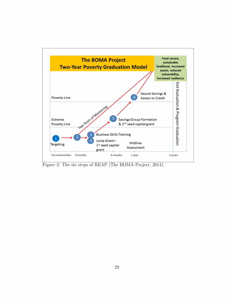
Figure 2: The six steps of REAP (The BOMA Project, 2014).

29

Figure 3: The quantile treatment effects of REAP.

30

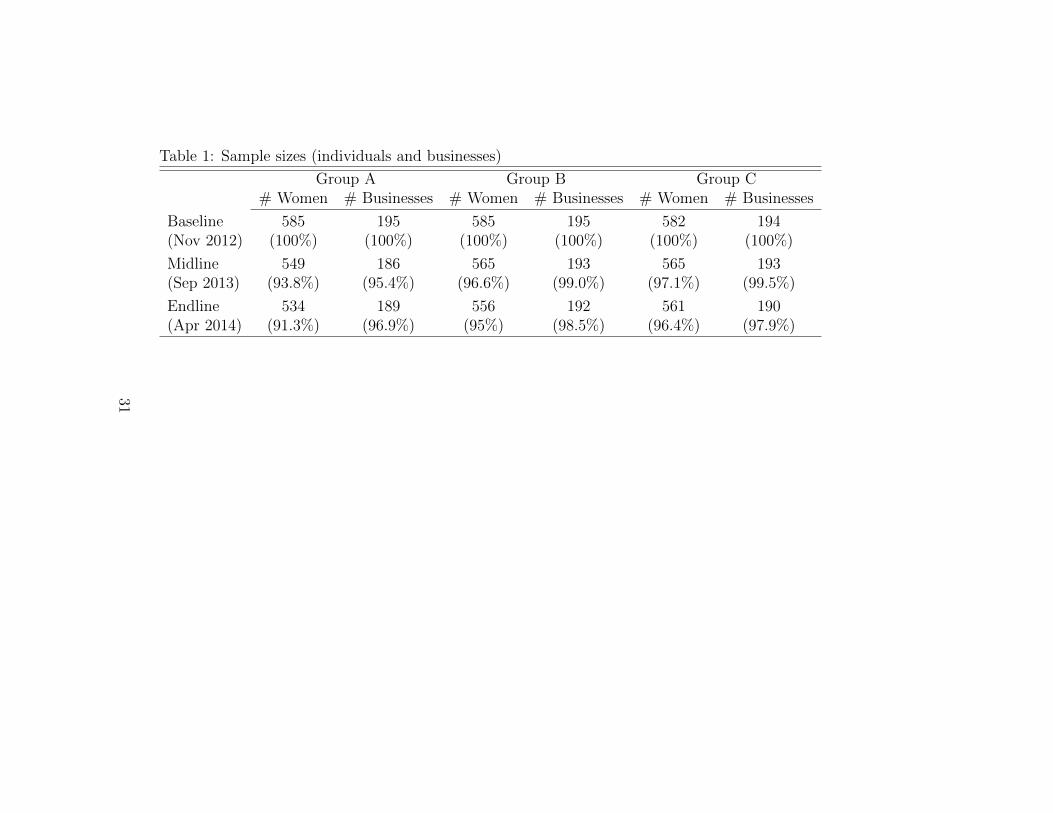
Table 1: Sample sizes (individuals and businesses)

Group A Group B Group C# Women # Businesses # Women # Businesses # Women # Businesses

Baseline 585 195 585 195 582 194(Nov 2012) (100%) (100%) (100%) (100%) (100%) (100%)

Midline 549 186 565 193 565 193(Sep 2013) (93.8%) (95.4%) (96.6%) (99.0%) (97.1%) (99.5%)

Endline 534 189 556 192 561 190(Apr 2014) (91.3%) (96.9%) (95%) (98.5%) (96.4%) (97.9%)

31

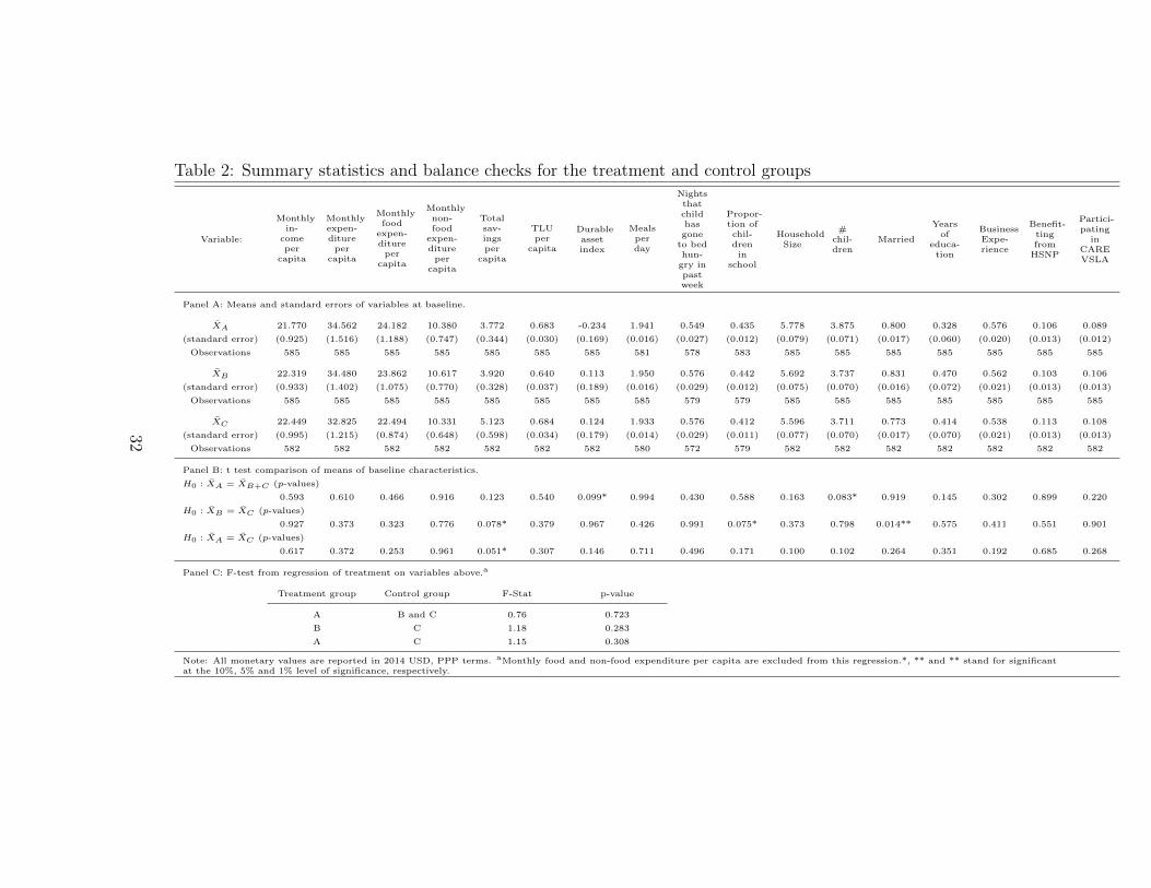
Table 2: Summary statistics and balance checks for the treatment and control groups

Variable:

Monthlyin-

comeper

capita

Monthlyexpen-diture

percapita

Monthlyfood

expen-diture

percapita

Monthlynon-food

expen-diture

percapita

Totalsav-ingsper

capita

TLUper

capita

Durableassetindex

Mealsperday

Nightsthatchildhasgone

to bedhun-

gry inpastweek

Propor-tion ofchil-drenin

school

HouseholdSize

#chil-dren

Married

Yearsof

educa-tion

BusinessExpe-rience

Benefit-tingfrom

HSNP

Partici-pating

inCAREVSLA

Panel A: Means and standard errors of variables at baseline.

X̄A 21.770 34.562 24.182 10.380 3.772 0.683 -0.234 1.941 0.549 0.435 5.778 3.875 0.800 0.328 0.576 0.106 0.089

(standard error) (0.925) (1.516) (1.188) (0.747) (0.344) (0.030) (0.169) (0.016) (0.027) (0.012) (0.079) (0.071) (0.017) (0.060) (0.020) (0.013) (0.012)

Observations 585 585 585 585 585 585 585 581 578 583 585 585 585 585 585 585 585

X̄B 22.319 34.480 23.862 10.617 3.920 0.640 0.113 1.950 0.576 0.442 5.692 3.737 0.831 0.470 0.562 0.103 0.106

(standard error) (0.933) (1.402) (1.075) (0.770) (0.328) (0.037) (0.189) (0.016) (0.029) (0.012) (0.075) (0.070) (0.016) (0.072) (0.021) (0.013) (0.013)

Observations 585 585 585 585 585 585 585 585 579 579 585 585 585 585 585 585 585

X̄C 22.449 32.825 22.494 10.331 5.123 0.684 0.124 1.933 0.576 0.412 5.596 3.711 0.773 0.414 0.538 0.113 0.108

(standard error) (0.995) (1.215) (0.874) (0.648) (0.598) (0.034) (0.179) (0.014) (0.029) (0.011) (0.077) (0.070) (0.017) (0.070) (0.021) (0.013) (0.013)

Observations 582 582 582 582 582 582 582 580 572 579 582 582 582 582 582 582 582

Panel B: t test comparison of means of baseline characteristics.

H0 : X̄A = X̄B+C (p-values)

0.593 0.610 0.466 0.916 0.123 0.540 0.099* 0.994 0.430 0.588 0.163 0.083* 0.919 0.145 0.302 0.899 0.220

H0 : X̄B = X̄C (p-values)

0.927 0.373 0.323 0.776 0.078* 0.379 0.967 0.426 0.991 0.075* 0.373 0.798 0.014** 0.575 0.411 0.551 0.901

H0 : X̄A = X̄C (p-values)

0.617 0.372 0.253 0.961 0.051* 0.307 0.146 0.711 0.496 0.171 0.100 0.102 0.264 0.351 0.192 0.685 0.268

Panel C: F-test from regression of treatment on variables above.a

Treatment group Control group F-Stat p-value

A B and C 0.76 0.723

B C 1.18 0.283

A C 1.15 0.308

Note: All monetary values are reported in 2014 USD, PPP terms. aMonthly food and non-food expenditure per capita are excluded from this regression.*, ** and ** stand for significantat the 10%, 5% and 1% level of significance, respectively.

32

Table 3: Testing for anticipation effects

Variable:

Monthlyincome per

capita

Monthlyexpenditureper capita

Totalsavings per

capita

TLU percapita

Durableasset index

Nights thatchild has

gone to bedhungry inpast week

Panel A: Means and standard errors of outcome variables for participants in groups B and C.

X̄B 26.263 49.906 3.683 1.031 2.014 0.463(standard error) (2.198) (1.949) (0.408) (0.052) (0.265) (0.058)

Observations 566 566 566 566 566 546

X̄C 23.437 51.703 3.178 1.119 2.086 0.565(standard error) (1.354) (2.191) (0.544) (0.057) (0.272) (0.044)

Observations 567 567 567 567 567 545

Panel B: t test comparison of means of outcome variables for participants in groups B and C.

H0 : X̄B = X̄C (p-values)0.274 0.540 0.458 0.254 0.848 0.163

Panel C: F-test from regression of treatment on variables above.

F-Stat p-value

0.99 0.432Note: All monetary values are reported in 2014 USD, PPP terms.

33

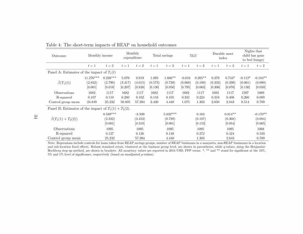
Table 4: The short-term impacts of REAP on household outcomes

Outcome: Monthly incomeMonthly

expenditureTotal savings TLU

Durable assetindex

Nights thatchild has goneto bed hungry

t = 1 t = 2 t = 1 t = 2 t = 1 t = 2 t = 1 t = 2 t = 1 t = 2 t = 1 t = 2

Panel A: Estimates of the impact of T1(t)

β̂(T1(t))

11.276*** 8.238*** 5.079 0.819 1.095 1.666** -0.016 0.205** 0.379 0.743* -0.112* -0.184**

(2.822) (2.790) (3.417) (4.015) (0.573) (0.739) (0.060) (0.100) (0.333) (0.399) (0.061) (0.080)

[0.001] [0.018] [0.207] [0.838] [0.130] [0.050] [0.795] [0.063] [0.306] [0.076] [0.130] [0.050]

Observations 1682 1117 1682 1117 1682 1117 1682 1117 1682 1117 1597 1089

R-squared 0.107 0.110 0.280 0.102 0.116 0.105 0.331 0.224 0.318 0.408 0.260 0.089

Control group mean 24.849 25.232 50.805 57.394 3.430 4.440 1.075 1.303 2.050 2.843 0.514 0.789

Panel B: Estimates of the impact of T1(1) + T2(2).

β̂(T1(1) + T2(2))

8.589*** -3.509 5.832*** 0.163 0.814** -0.170**

(2.232) (3.453) (0.789) (0.107) (0.368) (0.084)

[0.001] [0.310] [0.001] [0.153] [0.054] [0.065]

Observations 1095 1095 1095 1095 1095 1068

R-squared 0.127 0.126 0.148 0.272 0.424 0.103

Control group mean 25.232 57.394 4.440 1.303 2.843 0.789

Note: Regressions include controls for loans taken from REAP savings groups, number of REAP businesses in a manyatta, non-REAP businesses in a locationand sub-location fixed effects. Robust standard errors, clustered at the business group level, are shown in parentheses, while q-values, using the Benjamini-Hochberg step-up method, are shown in brackets. All monetary values are reported in 2014 USD, PPP terms. *, ** and ** stand for significant at the 10%,5% and 1% level of significance, respectively (based on unadjusted p-values).

34

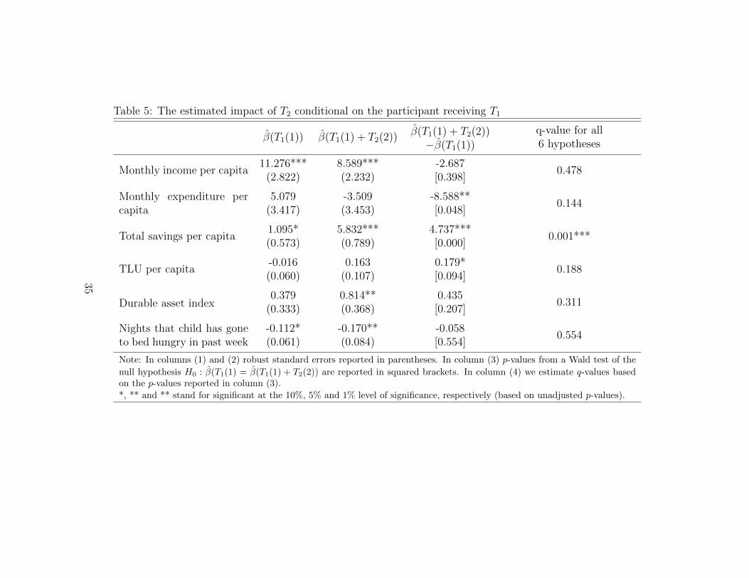
Table 5: The estimated impact of T2 conditional on the participant receiving T1

β̂(T1(1)) β̂(T1(1) + T2(2)) β̂(T1(1) + T2(2))−β̂(T1(1))

q-value for all6 hypotheses

Monthly income per capita11.276*** 8.589*** -2.687

0.478(2.822) (2.232) [0.398]

Monthly expenditure percapita

5.079 -3.509 -8.588**0.144

(3.417) (3.453) [0.048]

Total savings per capita1.095* 5.832*** 4.737***

0.001***(0.573) (0.789) [0.000]

TLU per capita-0.016 0.163 0.179*

0.188(0.060) (0.107) [0.094]

Durable asset index0.379 0.814** 0.435

0.311(0.333) (0.368) [0.207]

Nights that child has goneto bed hungry in past week

-0.112* -0.170** -0.0580.554

(0.061) (0.084) [0.554]

Note: In columns (1) and (2) robust standard errors reported in parentheses. In column (3) p-values from a Wald test of the

null hypothesis H0 : β̂(T1(1) = β̂(T1(1) + T2(2)) are reported in squared brackets. In column (4) we estimate q-values basedon the p-values reported in column (3).

*, ** and ** stand for significant at the 10%, 5% and 1% level of significance, respectively (based on unadjusted p-values).

35

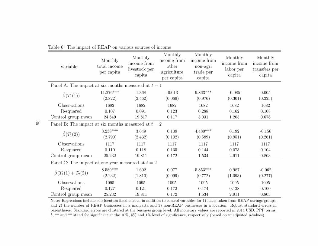
Table 6: The impact of REAP on various sources of income

Variable:

Monthlytotal incomeper capita

Monthlyincome fromlivestock per

capita

Monthlyincome from

otheragricultureper capita

Monthlyincome from

non-agritrade per

capita

Monthlyincome from

labor percapita

Monthlyincome fromtransfers per

capita

Panel A: The impact at six months measured at t = 1

β̂(T1(1))11.276*** 1.368 -0.013 9.863*** -0.085 0.005

(2.822) (2.462) (0.069) (0.976) (0.301) (0.223)

Observations 1682 1682 1682 1682 1682 1682

R-squared 0.107 0.091 0.123 0.288 0.162 0.108


Panel B: The impact at six months measured at t = 2

β̂(T1(2))8.238*** 3.649 0.109 4.480*** 0.192 -0.156

(2.790) (2.432) (0.102) (0.589) (0.951) (0.261)

Observations 1117 1117 1117 1117 1117 1117

R-squared 0.110 0.118 0.135 0.144 0.073 0.104


Panel C: The impact at one year measured at t = 2

β̂(T1(1) + T2(2))8.589*** 1.602 0.077 5.853*** 0.987 -0.062

(2.232) (1.810) (0.099) (0.772) (1.093) (0.277)

Observations 1095 1095 1095 1095 1095 1095

R-squared 0.127 0.121 0.172 0.174 0.128 0.100


Note: Regressions include sub-location fixed effects, in addition to control variables for 1) loans taken from REAP savings groups,and 2) the number of REAP businesses in a manyatta and 3) non-REAP businesses in a location. Robust standard errors inparentheses. Standard errors are clustered at the business group level. All monetary values are reported in 2014 USD, PPP terms.*, ** and ** stand for significant at the 10%, 5% and 1% level of significance, respectively (based on unadjusted p-values).

36

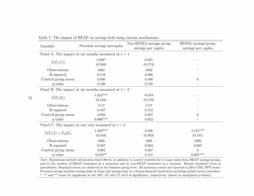
Table 7: The impact of REAP on savings held using various mechanisms.

Variable: Personal savings percapitaNon-BOMA savings group

savings per capitaBOMA savings group

savings per capita

Panel A: The impact at six months measured at t = 1

β̂(T1(1))1.038* 0.055 -

(0.568) (0.174) -

Observations 1682 1682 -

R-squared 0.119 0.098 -

Control group mean 3.030 0.400 0

q-value 0.136 0.750 -

Panel B: The impact at six months measured at t = 2

β̂(T1(2))1.624*** -0.010 -

(0.552) (0.170) -

Observations 1117 1117 -

R-squared 0.107 0.124 -


q-value 0.006*** 0.952 -

Panel C: The impact at one year measured at t = 2

β̂(T1(1) + T2(2))1.450*** 0.246 4.141***

(0.544) (0.303) (0.131)

Observations 1095 1095 1095

R-squared 0.087 0.063 0.605


q-value 0.012** 0.417 0.001***

Note: Regressions include sub-location fixed effects, in addition to control variables for 1) loans taken from REAP savings groups,and 2) the number of REAP businesses in a manyatta and 3) non-REAP businesses in a location. Robust standard errors inparentheses. Standard errors are clustered at the business group level. All monetary values are reported in 2014 USD, PPP terms.Personal savings includes savings kept at home and savings kept at a formal financial institution including mobile service providers.*, ** and ** stand for significant at the 10%, 5% and 1% level of significance, respectively (based on unadjusted p-values).

37

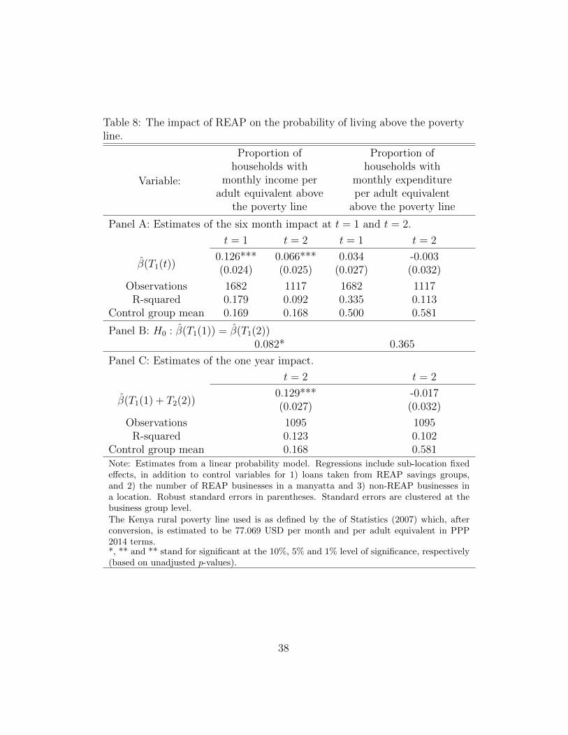
Table 8: The impact of REAP on the probability of living above the povertyline.

Variable:

Proportion ofhouseholds with

monthly income peradult equivalent above

the poverty line

Proportion ofhouseholds with

monthly expenditureper adult equivalent

above the poverty line

Panel A: Estimates of the six month impact at t = 1 and t = 2.

t = 1 t = 2 t = 1 t = 2

β̂(T1(t))0.126*** 0.066*** 0.034 -0.003(0.024) (0.025) (0.027) (0.032)

Observations 1682 1117 1682 1117R-squared 0.179 0.092 0.335 0.113

Control group mean 0.169 0.168 0.500 0.581

Panel B: H0 : β̂(T1(1)) = β̂(T1(2))0.082* 0.365

Panel C: Estimates of the one year impact.

t = 2 t = 2

β̂(T1(1) + T2(2))0.129*** -0.017(0.027) (0.032)

Observations 1095 1095R-squared 0.123 0.102

Control group mean 0.168 0.581Note: Estimates from a linear probability model. Regressions include sub-location fixedeffects, in addition to control variables for 1) loans taken from REAP savings groups,and 2) the number of REAP businesses in a manyatta and 3) non-REAP businesses ina location. Robust standard errors in parentheses. Standard errors are clustered at thebusiness group level.The Kenya rural poverty line used is as defined by the of Statistics (2007) which, afterconversion, is estimated to be 77.069 USD per month and per adult equivalent in PPP2014 terms.*, ** and ** stand for significant at the 10%, 5% and 1% level of significance, respectively(based on unadjusted p-values).

38

Table 9: The quantile treatment effects of REAP

OutcomeOLS

Estimates

10thpercentile

25thpercentile

50thpercentile

75thpercentile

90thpercentile

Panel A: Treatment effects at six months (at t = 1)

Monthly incomeper capita

11.276*** 2.446*** 5.041*** 6.753*** 10.266*** 9.292***

(2.822) (0.690) (0.933) (1.264) (1.997) (3.274)

Monthly expendi-ture per capita

5.079 1.357 0.882 1.195 3.222 3.307

(3.417) (1.130) (1.093) (1.586) (2.638) (4.605)

Total savings percapita

1.095* 0.000 0.000 -0.000 0.265*** 0.919***

(0.573) (0.000) (0.000) (0.000) (0.074) (0.353)

TLU per capita-0.016 0.011 0.007 0.000 0.000 -0.001

(0.060) (0.026) (0.030) (0.037) (0.056) (0.076)

Durable asset in-dex

0.379 -0.000 0.428 0.322 0.998** 0.622

(0.333) (0.317) (0.294) (0.334) (0.440) (0.498)

Panel B: Treatment effects at six months (at t = 2)


8.238*** 1.931** 2.560*** 2.393 6.610** 11.889***

(2.790) (0.795) (0.852) (1.605) (2.966) (4.331)


0.819 0.437 0.347 -0.259 -5.305 -8.576

(4.015) (1.732) (1.825) (2.377) (4.339) (8.033)


1.666** -0.000 -0.008 0.384 0.897 3.552***

(0.739) (0.216) (0.151) (0.378) (0.577) (1.018)

TLU per capita0.205** 0.055 0.097*** 0.102 0.195** 0.359**

(0.100) (0.036) (0.037) (0.065) (0.093) (0.151)


0.743* -0.167 0.036 0.650 0.944** 2.033***

(0.399) (0.389) (0.371) (0.494) (0.418) (0.746)

Panel C: Treatment effects at one year (at t = 2)


8.589*** 2.611*** 4.210*** 6.080*** 10.558*** 13.985***

(2.232) (0.985) (1.113) (1.485) (3.316) (5.318)


-3.509 -0.715 -1.960 -1.988 -6.689* -1.503

(3.453) (1.720) (1.669) (2.496) (3.564) (6.110)


5.832*** 2.744*** 3.566*** 4.826*** 6.636*** 8.139***

(0.789) (0.349) (0.294) (0.473) (0.820) (1.134)

TLU per capita0.163 0.081* 0.097** 0.106** 0.037 0.070

(0.107) (0.042) (0.044) (0.050) (0.111) (0.131)


0.814** -0.000 0.330 0.548 0.851 2.005***

(0.368) (0.390) (0.327) (0.371) (0.644) (0.549)

Note: Regressions include sub-location fixed effects, in addition to control variables for 1) loans taken from REAPsavings groups, and 2) the number of REAP businesses in a manyatta and 3) non-REAP businesses in a location.Robust standard errors in parentheses. Standard errors are clustered at the business group level. All monetaryvalues are reported in 2014 USD, PPP terms.

*, ** and ** stand for significant at the 10%, 5% and 1% level of significance, respectively.

39

Table 10: Overlap between individuals in the 90th percentile of the outcomedistribution

Outcome

Monthlyincome

per capita

Monthlyexpendi-ture percapita

Totalsavings

per capita

TLU percapita

Durableassetindex

Panel A: Overlap at six months (at t = 1)


1 0.254 0.148 0.231 0.183


1 0.195 0.166 0.195


1 0.112 0.225

TLU per capita 1 0.101


1

Panel B: Overlap at six months (at t = 2)


1 0.286 0.169 0.214 0.250


1 0.143 0.134 0.205


1 0.125 0.232



1

Panel C: Overlap at one year (at t = 2)


1 0.236 0.182 0.109 0.282


1 0.155 0.127 0.191


1 0.109 0.236



1

Note: Figures represent the proportion of overlap between individuals in the 90th percentile of the twocorresponding outcome distributions.

40

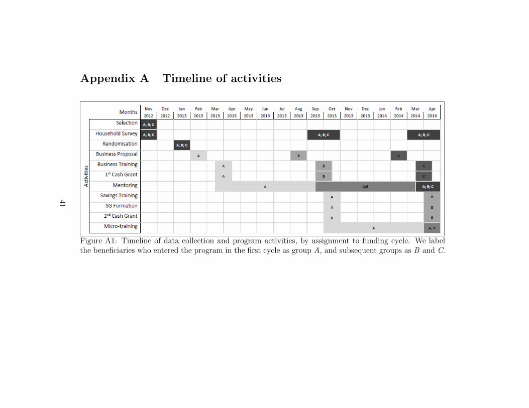
Appendix A Timeline of activities

Figure A1: Timeline of data collection and program activities, by assignment to funding cycle. We labelthe beneficiaries who entered the program in the first cycle as group A, and subsequent groups as B and C.

41

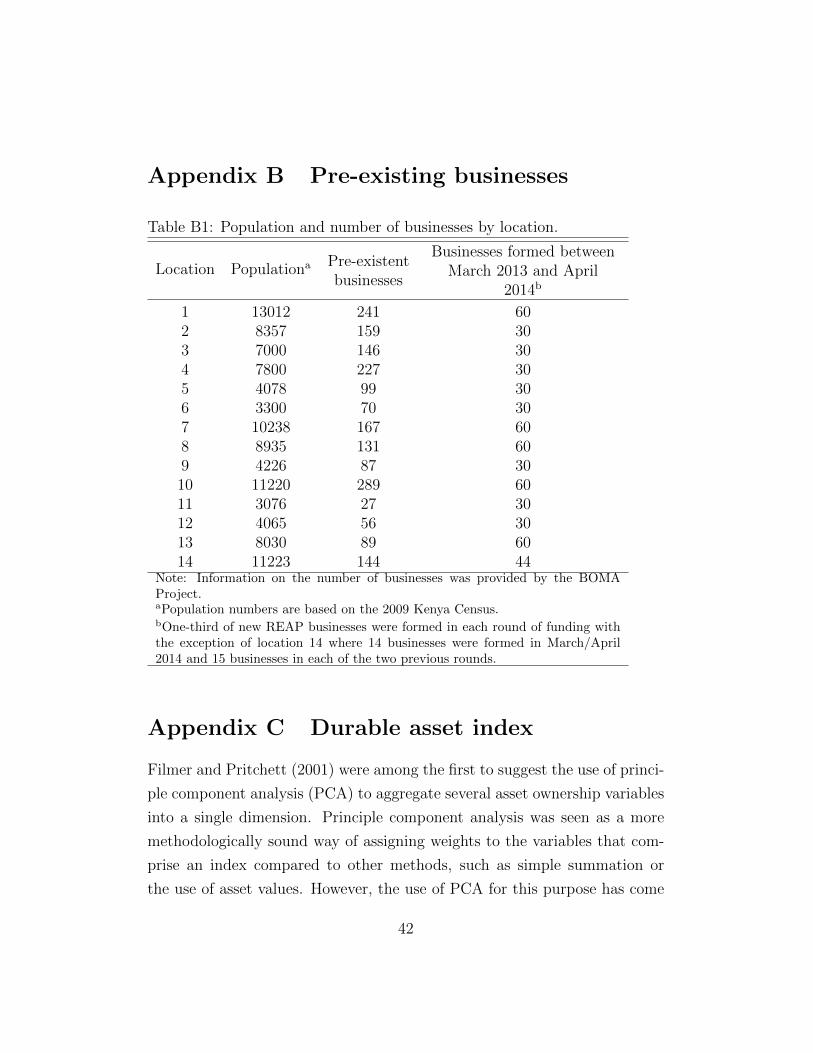
Appendix B Pre-existing businesses

Table B1: Population and number of businesses by location.

Location Populationa Pre-existentbusinesses

Businesses formed betweenMarch 2013 and April

2014b

1 13012 241 602 8357 159 303 7000 146 304 7800 227 305 4078 99 306 3300 70 307 10238 167 608 8935 131 609 4226 87 3010 11220 289 6011 3076 27 3012 4065 56 3013 8030 89 6014 11223 144 44

Note: Information on the number of businesses was provided by the BOMAProject.aPopulation numbers are based on the 2009 Kenya Census.bOne-third of new REAP businesses were formed in each round of funding withthe exception of location 14 where 14 businesses were formed in March/April2014 and 15 businesses in each of the two previous rounds.

Appendix C Durable asset index

Filmer and Pritchett (2001) were among the first to suggest the use of princi-

ple component analysis (PCA) to aggregate several asset ownership variables

into a single dimension. Principle component analysis was seen as a more

methodologically sound way of assigning weights to the variables that com-

prise an index compared to other methods, such as simple summation or

the use of asset values. However, the use of PCA for this purpose has come

42

under criticism since one of the assumptions underlying PCA is that vari-

ables are continuous and normally distributed which is violated when discrete

variables are included in the analysis (Howe, Hargreaves, & Huttly, 2008).

Multiple correspondence analysis (MCA) has been suggested as an alterna-

tive approach that is analogous to PCA but is better suited for use with

discrete data (Booysen et al., 2008).

We make use of the approach suggested by Booysen et al. (2008) to create

an asset index including information on the ownership of 11 durable assets

that were determined in all survey rounds. The assets include: 1) blanket,

2) flask, 3) kitchen, 4) lamp, 5) latrine, 6) mattress, 7) mobile phone, 8)

mosquito net, 9) nylon sheet, 10) slasher, and, 11) spade. Using the –mca–

command in Stata 13 we find that the first dimension accounts for 47% of the

inertia.30 We use the coordinates reported for the first dimension to generate

weights for every asset included in the index. These weights are reported in

Table C1.

30Inertia is Pearson’s chi-squared divided by sample size and is analogous to variancereported on in PCA.

43

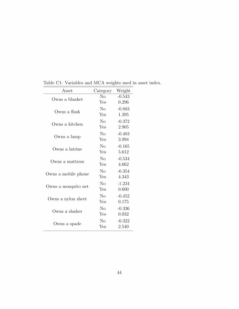
Table C1: Variables and MCA weights used in asset index.

Asset Category Weight

Owns a blanketNo -0.543Yes 0.296

Owns a flaskNo -0.883Yes 1.395

Owns a kitchenNo -0.372Yes 2.905

Owns a lampNo -0.483Yes 3.994

Owns a latrineNo -0.165Yes 5.612

Owns a mattressNo -0.534Yes 4.662

Owns a mobile phoneNo -0.354Yes 4.343

Owns a mosquito netNo -1.234Yes 0.600

Owns a nylon sheetNo -0.452Yes 0.175

Owns a slasherNo -0.336Yes 0.032

Owns a spadeNo -0.322Yes 2.540

44

all together now: the impact of a multifaceted approach to

Documents