allan variance ieee

IEEE Std 952™-1997 (R2008)

IEEE Standard Specification Format

Abstract: Specification and test requirements for a single-axis interferometric fiber optic gyro (IFOG)for use as a sensor in attitude control systems, angular displacement measuring systems, and angular ratemeasuring systems are defined. A standard specification format guide for the preparation of a single-axis IFOGis provided. A compilation of recommended procedures for testing a fiber optic gyro, derived from those pres-ently used in the industry, is also provided.

The Institute of Electrical and Electronics Engineers, Inc.

345 East 47th, New York, NY 10017-2394, USA

Authorized licensed use limited to: Aalborg Universitetsbibliotek. Downloaded on October 05,2010 at 08:50:36 UTC from IEEE Xplore. Restrictions apply.

AHtl»íísid ảỉpemimteí1 to lAâlSMSrUnSắiíslíelSíỉMPẾín IEEE XP|ore. Restrictions appiy.

IEEE Standards documents are developed within the IEEE Societies and the StandardsCoordinat-ing Committees of the IEEE Standards Board. Members of the committees serve voluntarily andwithout compensation. They are not necessarily members of the Institute. The standards developedwithin IEEE represent a consensus of the broad expertise on the subject within the Institute as wellas those activities outside of IEEE that have expressed an interest in participating in the develop-ment of the standard.

Use of an IEEE Standard is wholly voluntary. The existence of an IEEE Standard does not implythat there are no other ways to produce, test, measure, purchase, market, or provide other goodsandservices related to the scope of the IEEE Standard. Eurthermore, the viewpoint expressed at thetime a standard is approved and issued is subject to change brought about through developments inthe state of the art and comments received from users of the standard. Every IEEE Standard is sub-jected to review at least every Fve years for revision or reaffirmation. When a document is morethan Fve years old and has not been reaffirmed, it is reasonable to conclude that its contents,although still of some value, do not wholly reflect the present state of the art. Users are cautionedtocheck to determine that they have the latest edition of any IEEE Standard.

Comments for revision of IEEE Standards are welcome from any interested party, regardless ofmembership aíhliation with IEEE. Suggestions for changes in documents should be in the form ofaproposed change of text, together with appropriate supporting comments.

Interpretations: Occasionally questions may arise regarding the meaning of portions of standardsasthey relate to specihc applications. When the need for interpretations is brought to the attention ofIEEE, the Institute will initiate action to prepare appropriate responses. Since IEEE Standards rep-resent a consensus of all concerned interests, it is important to ensure that any interpretation hasalso received the concurrence of a balance of interests. Eor this reason, IEEE and the members ofitssocieties and Standards Coordinating Committees are not able to provide an instant response to

Secretary, IEEE Standards Board445 Hoes LanePO. Box 1331Piscataway, NJ 08855-1331

USA

Note: Attention is called to the possibility that implementation of this standard mayrequire use of subject matter covered by patent rights. By publication of thisstandard,no position is taken with respect to the existence or validity of any patent rights inconnection therewith. The IEEE shall not be responsible for identifying patents forwhich a license may be required by an IEEE standard or for conducting inquiriesinto

Authorization to photocopy portions of any individual standard for internal or personal use isgranted by the Institute of Electrical and Electronics Engineers, Inc., provided that the appropriatefee is paid to Copyright Clearance Center. To arrange for payment of licensing fee, please contactCopyright Clearance Center, Customer Service, 222 Rosewood Drive, Danvers, MA 01923 USA;(508) 750-8400. Permission to photocopy portions of any individual standard for educationalclass-room use can also be obtained through the Copyright Clearance Center.

AHtl»íisid ểtíseliiaiíe1 to lAâlSMSrUnSắiíslíelSíỉMPẾín Pío'wa|ỹiideíbsra(?cịo!?«c0?iêẼltXal)0ỉ:;Rìẩ6fclrffi<?ííỄPm' IEEE xp|ore- Restrictions apply.

D. Anderson s. Bennett, Chair

T. FuhrmanR. Morrow

M. Ash F. Garcia G. Murray*C. Barker B. Katz J.

NeugroschiJ. Beri J. Kieffer R. Peters*S. Bongiovanni M. Koning L.

RichardsonP Bouniol L. Kumar G. ShawJ. Brewer K. Lantz P Simpson

Introduction

(This introduction is not a part of IEEE Std 952-1997, IEEE Standard Specification Eormat Guide and TestProcedure forSingle-Axis Interferometric Eiber Optic Gyros.)

This Standard was prepared by the Gyro and Accelerometer Panel of the IEEE Aerospace and ElectronicSystems Society and consists of two parts.

Part I is a specification format guide for the preparation of a single-axis interferometric fiber optic gyro(IEOG) specification. It provides a common meeting ground of terminology and practice for manufacturersand users. The user is cautioned not to over specify; only those parameters that are required to guaranteeproper instrument performance in the specidc application should be controlled. In general, the specificationshould contain only those requirements that can be verided by test or inspection. Parameters in addition tothose given in this standard are not precluded.

Part II is a compilation of recommended procedures for testing a single-axis IEOG. These procedures,including test conditions to be considered, are derived from those currently in use. Eor a specidc application,the test procedure should reflect the requirements of the specidcations; therefore, not all tests outlined in thisstandard need to be included, nor are additional tests precluded. In some cases, alternative methods for mea-suring performance characteristics have been included or indicated.

The intent is for the specidcation writer to extract the applicable test conditions and equipment requirementsfrom Clause 11 for inclusion in the appropriate subclauses listed under 6.5. Similarly, it is intended that thewriter extract the applicable test procedures from Clause 12 for inclusion in the appropriate subclauses listedunder 6.6. Part II can also be used as a guide in the preparation of a separate gyro test specidcation withappropriate clause numbering. In general, the intent is for the Part II test procedure to refer to Part I require-ments for performance, mechanical, electrical, environmental, reliability, and quality assurance. To that end,a test should not be listed in Part II unless a related requirement exists in Part I.

Blank spaces in the text of this standard permit the specidcation writer to insert specidc information such asparameter values and their tolerances, clause numbers, etc. Brackets are to be used to enclose alternativechoices of dimensional units, signs, axes, etc. Boxed statements are included for information only and arenot part of the specidcation or test procedures. The terminology used conforms to IEEE Std 100-1996 andIEEE Std 528-1994. The units used conform to ANSI 268-1992. The abbreviation of units conforms to IEEEStd 260.1-1993. The graphic symbols used conform to IEEE Std 315-1975.

This standard defines the requirements and test procedures for an IEOG in terms unique to that gyro. Therequirements contained in this standard cover application where the gyro is used as an angular motion sensorin navigation and control systems.

The term “interferometric fiber optic gyro” is accepted to include the electronics necessary to operate thegyro and to condition the output signal.

Annex A lists various gyro design features for which this format is applicable. The table therein is notintended to make any suggestions regarding the selection of particular design features that might restrict thefree choice of manufacturers.

Annex B is an overview of dynamic and stochastic modeling.

Annex C is an overview of noise process variance analysis as a method for determination of the drift ratecoefficients and the quantization coefficient.

Copyright © 1998 IEEE. All rights reserved.

iii

This Standard represents a large scale, group effort. More than 116 individuals attended over 40 meetings ofthe Gyro and Accelerometer Panel during preparation of this standard. The following persons were on theGyro and Accelerometer Panel:

H. Califano T. Lear* T. StanleyA. Campbell* D. Lynch C. SwansonJ. D’Angelo R. Marquess L. ThielmanG. Erickson H. Morris L. TrozpekJ. Ficalora G. Morrison* B. Wimber*S. Finken B. YoumansD. Anderson S. Finken G. NeugebauerW. Armstrong T. Fuhrman P PalmerM. Ash K. Homb R. PetersC. Barker B. Katz F. PetriS. Bennett J. Kieffer G. ShawS. Bongiovanni L. Kumar C. SwansonP Bouniol J. Mackintosh M. TehraniJ. Brewer E. Mettler L. ThielmanH. Califano H. Morris C. TrainorA. Campbell G. Morrison B. WimberJ. D’Angelo R. Morrow D. WinkelG. Erickson B. YoumansWhen the IEEE Standards Board approved this standard on 16 September 1997, it had the followingmembership:

Donaid c. Loughry, Chair Richard J. Hoiieman, Vice ChairAndrew G. Salem, Secretary

Clyde R. Camp Lowell Johnson Louis-Fran9ois Pau

Stephen L. Diamond Robert Kennelly Gerald H. PetersonHarold E. Epstein E. G. “Al” Kiener John W. PopeDonald C. Fleckenstein Joseph L. Koephnger* Jose R. RamosJay Forster* Stephen R. Lambert Ronald H. ReimerThomas F. Garrity Lawrence V. McCall Ingo RuschDonald N. Heirman L. Bruce McClung John S. RyanJim IsaakBen C. Johnson

Marco W. Migliaro Chee Kiow TanHoward L. Wolfman

AHtlìOíí§id ibinsed ảỉpemimteí1 to lAâlSMSrUnSắiíslíelSíỉMPẾín IEEE xp|ore- Restrictions appiy.

*Former Chair

The following persons were on the balloting committee:

*Member Emeritus

Also included are the following nonvoting IEEE Standards Board liaisons:

Satish K. AggarwalAlan H. Cookson

Kim Breitfelder

iv Copyright © 1998 IEEE. All rights

reserved.

AHtl»íisid ảỉpemimteí1 Ito ^ẵl&PtíarảSSâtsíỉẽtiĩntíầliotPíkn IEEE XP|ore. Restrictions apply.

Contents

1. Overview .............................................................................................................................................. 1

1.1 Scope ............................................................................................................................................ 1

2. Reíerences ............................................................................................................................................. 1

Part I—Specification format .......................................................................................................................... 2

3. Deíinitions ............................................................................................................................................ 2

4. Applicable documents .......................................................................................................................... 2

4.1 Speciíications ............................................................................................................................... 2

4.2 Standards ..................................................................................................................................... 3

4.3 Drawings ...................................................................................................................................... 3

4.4 Bulletins ....................................................................................................................................... 3

4.5 Other publications ....................................................................................................................... 3

5. Requirements ........................................................................................................................................ 4

5.1 Description ................................................................................................................................... 4

5.2 General requirements ................................................................................................................... 4

5.3 Períormance ................................................................................................................................. 4

5.4 Mechanical requirements ............................................................................................................. 8

5.5 Electrical requirements..............................................................................................................10

5.6 Environmental requirements ...................................................................................................... 12

5.7 Reliability..................................................................................................................................17

6. Quality assurance provisions .............................................................................................................. 18


AHtlìOíí§id ảỉpemimteí1 Ito lAâlÈPdíartóiSst isiỉgtsbìtìayietPkn IEEE XP|ore. Restrictions appiy.

11. Test conditions and test equipment....................................................................................................25

11.1 Standard test conditions...........................................................................................................25

11.2 Standard operating and test equipment....................................................................................27

12. Test procedures...................................................................................................................................27

12.1 Examination of product—Mechanical ..................................................................................... 27

12.2 Examination of product—Electrical ........................................................................................ 27

12.3 Leak test ................................................................................................................................... 29

12.4 Input power .............................................................................................................................. 30

12.5 Turn-on time ............................................................................................................................ 30

12.6 Warm-up time .......................................................................................................................... 31

12.7 Polarity .................................................................................................................................... 31

12.8 Operating temperature test series ............................................................................................ 32

vi


1ANSI publications are available from the Sales Department, American National Standards Institute, 11 West 42nd Street, 13th Floor,New York, NY 1OO36, USA.

2IEEE publications are available from the Institute of Electrical and Electronics Engineers, 445 Hoes Lane, P.O. Box 1331, Piscataway,NJ O8855-1331, USA.

AHtlìOíí§id ảỉpemimteí1 Ito ^ẵl&PtíarảSSâisíỉẽtiĩntíầlioíPíkn IEEE xp|ore- Restrictions apply.

IEEE Standard Speci.cation Format

1. Overview

2. References

This standard shall be used in conjunction with the following publications. When the following standardsaresuperseded by an approved revision, the revision shall apply.

ANSI 26O.1-1993 American National Standard Letter Symbols for Units of Measurement (SI Units, Cus-tomary Inch-Pound Units, and Certain Other Units).1

IEEE/ASTM SI 1O-1997, Standard for Use if the International System of Units (SI): The Modern MetricSystem.2


1.1 Speci.cations

1.1.1 Government

3IEEE Std 812-1984 has been withdrawn; however, copies can be obtained from Global Engineering, 15 Inverness Way East, Engle-wood, CO 8O112-57O4, USA, tel. (3O3) 792-2181. 2

AHtliOíí§id Ito ^ẵl&PtíarảSSâisíỉẽtiĩntíầliotPíkn Pío'wa|ỹiideíbsra(?cịo!?ftic0?iêẼltXal)0ỉ:;Rìẩ6fclrffi<?ííỄPm' IEEE XP|ore. Restrictions apply.

IEEEstd 952-1997 IEEE STANDARD SPECIFICATION FORMAT GUIDE AND TEST PROCEDURE

IEEE Std 315-1975 (Reaff 1993), IEEE Graphic Symbols for Electrical and Electronics Diagrams (ANSI/DoD).

IEEE Std 315A-1986 (Reaff 1993), IEEE Supplement to Graphic Symbols for Electrical and ElectronicsDiagrams (ANSI/DoD).

IEEE Std 528-1994, IEEE Standard for Inertial Sensor Terminology (ANSI).

IEEE Std 812-1984, IEEE Standard Definitions of Terms Relating to Fiber Optics.3

Part l—Speci.cation íormat

3. De.nitions

3.2 Applicable documents

Give identification number, title, date of issue, and revision letter of each listed document.

MIL-P116J Methods of Preservation 1 October 1991.

3.2.1 Industry/Technical

2 Copyright © 1998 IEEE. All rights reserved.

AHtl»írgld licsnsed ảỉpemimteí1 to E^§!&ft(í9rảSWâfsíỉ§!SlíifelÌ®tffen Kft'WSlỹlldedjSra(?Cị9:l?fttdm?iêẼI0<a,b0ỉ:;P0âfìfclrffi^íÍỄPIỊ' IEEE XP|ore. Restrictions apply.

FOR SINGLE-AXIS INTERFEROMETRIC FIBER OPTIC GYROSIEEE

Std 952-1997

3.3 Standards

3.3.1 Government

MIL-STD-1O5E Sampling Procedure and Tables for Inspection by Attributes 1 February 1995.

MIL-STD-461D Electromagnetic Interference Characteristics, Emission and Susceptibility January 1993Requirements for the Control of Electromagnetic Interference.

MIL-STD-462D+ Electromagnetic Interference Characteristics, Measurements of 1 April 1995.

MIL-STD-7O4E Aircraft Electric Power Characteristics January 1991.

MIL-STD-74OB Airborne and Structure borne Noise Measurements and Acceptance 1 June 1965 Criteriaof Shipboard Equipment.

MIL-STD-781D Reliability Design Qualibcation and Production Acceptance Tests: October 1986 Expo-nential Distribution.

MIL-STD-785B Reliability Program for Systems and Equipment Development and Notice 2 Production2 August 1988.

MIL-STD-81OE Environmental Test Methods and Engineering Guidelines 2 September 1993.


IEEE Std 1OO-1996, IEEE Standard Dictionary of Electrical and Electronics Terms.

IEEE Std 528-1994, IEEE Standard for Inertial Sensor Terminology.

3.3.3 Company

3.4 Drawings

3.4.1 Government


3.4.3 Company

3.5 Bulletins

3.5.1 Government


4. Requirements

4.1 Description

To -ll in the blanks, refer to Annex A for examples.

4.2 General requirements

4.2.1 Precedence

In the event of conhict among the purchase agreement, this specihcation, and other documents referred to inthis specihcation, the order of precedence shall be as follows:

a) Purchase agreement.

b) This specihcation and its applicable drawings (see 5.4.2 and 5.5.1).

When required by the application, the sensitivity of a gyro characteristic to variations in voltage, fre-quency, temperature, or other variables should be included in the subclause specifying that characteristic.

4.3.1 Input rate limits

4.3.1.1 Maximum

The input rate limits about the gyro input axis (IA) shall be ±__________[°/s, rad/s].

The positive and negative input rate limits need not be equal. Multiple rate limits may be speci-ed.

4.3.1.2 Minimum (dead band)

The gyro dead band shall not exceed__________[°/s, rad/s].

4.3.2 Gyro scale factor, s__________["/p, $rad/p,______] +____________j. 4

In the angular rate sensing mode, the scale factor is normally speci-ed in (°/h)/V, (°/h)/Hz. In theangulardisplacement sensing mode, the scale factor is normally speci-ed in "/p. Different values and tolerancesmay be speci-ed for different input ranges.

The scale factor range includes the manufacturing tolerance. The test procedure will result in a nominalscale factor that is de-ned in the model equation in 8.3.

4 Copyright © 1998 IEEE. All rights reserved.

AHtliOíí§id ảỉpemimteí1 Ito ^ẵl&PtíarảSSMSíỉẽtiĩntíầliotPíkn IEEE xp|ore- Restrictions apply.

1.1.2 Drift rate, D, E

1.1.2.1 Bias and random, D

1.1.2.1.1 Bias, DF

__________±____________°/h.

Repeatability.___________°/h [maximum spread, lơ,_______].

Thermal cycles and other environmental exposures, shutdowns, time between runs, remounting, and addi-tional factors pertinent to the particular application should be specihed.

AHtl»írgld licsnsed ảỉpemimteí1 ito E^§!&ft(í9rảSWâfsíỉ§!SlíifelÌ®tffen Kft'WSlỹlldedjSra(?Cị9:l?fttdm?iêẼI0<a,b0ỉ:;P0âfìfclrffi^íÍỄPIỊ' IEEE XP|ore- Restrictions apply.


Std 952-1997

4.3.2.1 Gyro scale factor errors

a) Linearity Error.___________[ppm, %] of full scale and/or____________[ppm, %] of output, [maxi-

Scale factor linearity error may have a component periodic in rate due to optical feedback to the source.

b) Asymmetry. The difference between the scale factor measured with positive input rates and negative

input rates shall not exceed___________[ppm, %] of half the sum of the magnitudes of the scale fac-

tor determined for positive and negative inputs.

Repeatability involves changes in scale factor that occur between periods of operation. Thermal cyclesand other environmental exposures, shutdowns, time between runs, remounting, and additional factorspertinent to the particular application should be specihed.

d) Stability. ___________ [ppm, %], [maximum spread, lơ, ________] for ____________ [hours, days,

______].

4.3.2.2 Gyro scale factor sensitivities

a) Temperature. The change in gyro scale factor resulting from a change in steady-state operating tem-

perature shall not exceed____________ppm from that measured at_____________°c over the range

___________°c to___________°c.

Additional sensitivities may be specihed such as those due to variations in supply voltage, rate oftemper-ature change, temperature gradient, orientation, acceleration, vibration, magnetic held, radiation, andother environments pertinent to the particular application.


5

AHtlìOíí§id ảỉpemimteí1 Ito ^ẵl&PtíarảSSâtsíỉẽtiĩntíầliotPíkn IEEE xp|ore- Restrictions apply.


5.3.3.1.2 Random, D

Random drift rate is usually defined in terms of the Allan variance components. Thesecomponentsshould be specihed. See DR terms under 8.3 and Annex c.

a) Angle random walk (rate white noise) coefficient, N._____°/h1/2 maximum.

b) Bias instability coefficient, B._____°/h maximum.

c) Rate random walk coefficient, K._____(°/h)/h1/2 maximum.

For some applications it may be sufficient to dehne random drift as the standard deviation of theoutput.The time interval and integration time should be specihed.

5.3.3.1.3 Measurement noise, DQ

Quantization noise coefficient, Q______[", $rad] maximum.

Measurement noise is usually dehned as the Allan variance component Q. See 8.3 and Annex c.

5.3.3.2 Environmentally sensitive,

E

5.3.3.2.1 Thermal

a) Temperature. The change in gyro bias resulting from a change in steady-state operating temperature

shall not exceed___________°/h from that measure at____________°c over the range____________

°c to____________°c.

The characteristics of the ramp should be representative of the intended application.

c) Time-dependent temperature gradient. The maximum change in gyro bias resulting from a change intemperature ramp of___________°c/min shall not exceed____________°/h.

The magnitude of the temperature ramp should be representative of the intended application. This isintended to specify the bias error associated with the Shupe effect, which arises from the time-dependenttemperature gradient with respect to the center of the hber length. The magnitude of the effect is depen-dent on gyro design, including coil-winding techniques and thermal packaging, and exhibitsdifferencesdepending on the direction of thermal input. The mounting arrangements and method of thermal input

5.3.3.2.2 Magnetic

The change in gyro bias resulting from a change in steady-state flux density shall not exceed__________°/h

over the range___________to____________[mT, G,_______].

Gyro axis and characteristics of the held should be dehned. If exposure to a varying held is required,thenature of the variation should be described. Demagnetization may be necessary following exposure.

6 Copyright © 1998 IEEE. All rights

reserved.

AHtlìOíí§id licensed ảỉpemimteí1 Ito ^ẵl&PtíarảSSMSíỉẽtiĩntíầliotPíkn IEEE xp|ore- Restrictions apply.


Std 952-1997

5.3.3.2.3 Other sensitivitiesAdditional sensitivities may be specibed such as those due to variations in supply voltage, rate of temper-ature change, orientation, acceleration, vibration, radiation, and other environments pertinent to the par-ticular application.

5.3.4 IA alignment characteristics

5.3.4.1 IA misalignment

__________[', mrad], maximum with respect to the input reference axis (IRA).

The specibc direction of IA misalignment may be important in some applications and should bespecibedwith respect to XRA and YRA gyro case reference axes. Note that these axes are defined in 5.4.3.

5.3.4.2 IA alignment repeatability

__________[", $rad], [maximum spread, lơ,_______].

Thermal cycles and other environmental exposures, shutdowns, time between runs, remounting, andaddi-tional factors pertinent to the particular application should be specibed.

5.3.4.3 IA alignment sensitivitiesIA alignment sensitivities may be specibed, such as those due to temperature, thermal gradients, rate oftemperature change, acceleration, vibration, and additional environments pertinent to the particular appli-cation.

5.3.5 Operating temperature

The operating temperature above applies only to temperature-controlled gyros. For gyros intended tooperate without temperature control, see 5.6.4.4.

5.3.6 Warm-up time[s,______], maximum.

The limits of gyro performance during that portion of warm-up time following the turn-on time shouldbespecibed for certain applications. These limits could be fixed bounds or functions of time. More thanonefunction may be specibed for different temperatures at the time of turn-on, or different functions may

5.3.7 Turn-on time

The gyro output rate shall be within___________[°/h] of the input rate within____________[s,_______] after

AHtliOíí§id licensed ảỉpemimteí1 Ito ^ẵl&PtíarảSSMSíỉẽtiĩntíầliotPíkn IEEE xp|ore- Restrictions apply.


5.3.8 Polarities

5.3.8.1 Input axis (IA)

The positive IA shall conform to [drawing number___________A Figure__________].

5.3.8.2 Output signals

The output signals representing gyro rotation shall conform to [drawing number ________________A Figure

__________].

5.3.9 Reference constants

These constants are for reference only. They are not specihed independently, because they may varywithin the framework of the specihcation, or because they are difficult or impossible to measureindepen-dently in a complete gyro. Nominal values are listed.

5.3.9.1 Light source wavelength

5.3.9.3 Effective area per turn

__________[m2,______].

5.3.9.4 Physical pathlength

__________[m,_______].

4.4 Mechanical requirements

Mechanical characteristics shall be as specihed hereinafter.

4.4.1 Exterior surface

Additional requirements controlling surface hnish, workmanship, processing, etc., may be specihed.

4.4.2 Outline and mounting dimensions

Outline and mounting dimensions, and accuracy requirements of mounting surface shall conform to [draw-

8

1.1.3 Seal

The gyro shall be sealed such that the equivalent helium leak rate is less than_____________[cm3/s,_______]

when subjected to a pressure of______________ ± ___________ Pa and gyro temperature of_____________

±__________°c for a minimum of____________minutes.

AHtl»írgld licsnsed ểmMtgd ito E^§l&ft(í9rảSWâfsíỉ§!SlíifelÌ®tffen Kft'WSlỹlldedjSra(?Cị9:l?fttdm?iêẼI0<a,b0ỉ:;P0âfìfclrffi^íÍỄPIỊ' IEEE XP|ore- Restrictions apply.


Std 952-1997

4.4.3Gyro

axes

The X gyro case reference axis (XRA) and Y gyro case reference axis (YRA) are mutually perpendicularand are located by means of the gyro mounting surface and the reference index on the gyro case [notch, pin,

scribe line,______]. The IRA, XRA, and YRA are reference axes de-ned with respect to the mounting provi-

sions. These axes are nominally parallel to IA, XA, and YA respectively, and de-ne a right-handed coordi-nate system. The IRA is perpendicular to the gyro mounting surface and shall conform to [drawing number

YA YRA

XA

XRA

Figure 1—Gyro axes and misalignment angles

4.4.4 Weight

__________+____________[g,______].

Specify those components such as cables, connectors, and electronics that are to be included in the weight.


9

AHtl»írgld licsnsed ảỉpemimteí1 ito E^§l&ft(í9rảSWâfsíỉ§!SlíifelÌ®tffen Kft'WSlỹlldedjSra(?Cị9:l?fttdm?iêẼI0<a,b0ỉ:;P0âfìfclrffi^íÍỄPIỊ' IEEE XP|ore- Restrictions apply.


4.4.5 Identi.cation of product

The gyro shall be identihed on the surface and in the manner indicated in drawing number_________

Identihcation shall include the following:

a) Fiber optic gyro or IFOG

b) Specihcation number

c) Unit serial number

The purchase agreement may require additional identihcation such as date of manufacture and safetywarnings.

4.4.6 Acoustic noise

The acoustic noise emissions shall conform to

4.5 Electrical requirements

Electrical characteristics shall be as speci-ed in this subclause.

4.5.1 Schematic

The electrical circuits shall be connected as shown in [drawing number___________A Figure__________].

The schematic may include preamplihers, temperature sensing circuits, heater circuits, trim components,test points, etc.

4.5.2 Impedances

The gyro impedances shall be___________&.

4.5.3 Input power

The input power shall not exceed___________w.

Requirements such as power factor for each circuit, frequency, voltage, ripple, starting, and operatingcur-rent should be speci-ed. Transient conditions may need to be speci-ed.

Gyros with environmental controls may exhibit substantial changes in input power requirements overthe

10

1.1.4 Temperature sensors

The output of the temperature sensor(s) shall be____________±____________[&, V,_______] in the operating

temperature range specihed in 5.6.4.4 of this standard. The temperature rise of the sensor due to self-heating

shall not exceed____________°C at___________mA. The scale factor of the temperature sensor(s) shall be

[±]___________±___________[V/°C,_______].

1.1.5 Insulation resistance

The insulation resistance between isolated interface circuits and between the case(s) and circuits isolated

from the case(s) shall not be less than______________M& measured at_____________ ±___________V dc,

applied for___________±____________s.

AHtl»íisid ảỉpemimteí1 Ito ^ẵl&PtíarảSSâtsíỉẽtiĩntíầliotPíkn IEEE XP|ore- Restrictions apply.


Std 952-1997

4.5.4Test

po

n

s

Test points required for monitoring and testing of the gyro should be specihed. These may include excita-tion voltages, other control signals, or temperature sensor(s). Any special buffering or scaling require-ments should be specihed.

4.5.5 GroundingElectrical grounding design requirements (for example, requirements for isolation between input, outputpower returns and the grounding requirements for shields, chassis and critical components) should bespecihed.

4.5.6 Output signals

The type and characteristics of output signal(s) required, such as analog voltage or current, parallel orserial digital, or incremental angle pulses should be specihed. For example:

Type: Pulses indicating positive angular increments on one signal line and pulses indicating negativeangular increments on a second line.

Characteristics:

Source impedanceLoad impedanceWave shape (see Figure 2)

Maximum pulse rate

Thermistors, thermocouples, or other temperature sensors may be specihed. Temperature sensors maybebuilt into the gyro for use in characterizing its temperature sensitivity. If sensors are required, specifyquantity, locations, and characteristics. The temperature range over which the scale factor should bespec-

Different voltages may be specihed for different circuits.


11

1.1.6 Electromagnetic interíerence

The electromagnetic emissions and susceptibilities shall conform to

1.1.7 Storage

The gyro shall conform to all requirements of this specibcation after exposure to the following environmentsor speci-ed combinations thereof, while packaged as speci-ed in Clause 7.

1.1.8 Transport

The gyro shall conform to all requirements of this specibcation after exposure to the following environments

or speci-ed combinations thereof, while packaged as speci-ed in Clause 7.


UNITS MAXIMUM MINIMUM REMARKS

V" volts Steady-state low voltage

v2 volts N/A Overshoot voltage

VQ volts N/A Undershoot voltage

V' volts Steady-state high voltage

V] volts N/A Maximum low voltage transient

tr seconds Rise time

tf seconds Fall time

IEEE

std 952-1997 IEEE STANDARD SPECIFICATION FORMAT GUIDE AND TEST PROCEDURE

4.5.7 Dielectric strength

The leakage current shall not exceed ______________ nA when ____________ ± ____________ V RMS, at

___________Hz, are applied between isolated interface circuits, and between the case(s) and circuits isolated

Different voltages may be speci-ed for different circuits. In some instances, lower voltages may bespec-i-ed for subsequent tests.

Describe the requirements. In the United States, a common standard is MIL-STD-461.

4.5.8 Electromagnetic compatibilityDescribe the requirements. In the United States, a common standard is MIL-STD-461.

4.6 Environmental requirements

This subclause contains environmental requirements only. Test procedures that are to be used,includingrequired combinations of environments, are covered in 6.6 of this standard.

The procuring organization should list the applicable environments from 5.6.4 of this standard andspec-ify the limits for each based on the storage conditions expected.

The procuring organization should list the applicable environments from 5.6.4 of this standard andspec-ify the limits for each based on the transportation conditions expected.

4.6.1 OperationIn order to properly specify the environmental requirements for a gyro, three different sets of environ-ments or environmental limits, or both, as de-ned in 5.6.3.1, 5.6.3.2, and 5.6.3.3 of this standard mayneed to be described.

12


Std 952-1997

t" seconds Turn-on transient time

t2 seconds High voltage on time

N/A Ratio of turn-on transient torequired on time

T

‘M/T

secondsWaveform period

Duty cycle

AHtl»íisid licsnsed ểtíseliiaiíe1 to IEEE XP|ore- Restrictions apply.

Figure 2—Wave shape requirements for direct coupled pulse-type signals

4.6.1.1 Operating environment

The gyro shall conform to all requirements of this specihcation during exposure to the following environ-

Where degraded performance is to be allowed, include the parenthetical phrase in 5.6.3.1 of thisstandardand list in the blank space those environments for which degraded performance is allowed. Theprocuringorganization should list the applicable environments from 5.6.4 of this standard and specify the limitsfor

1.1.8.1 Survival environment, nonoperating

The gyro shall conform to all requirements of this specihcation after the nonoperating gyro has beenexposed to the following environments or speci-ed combinations thereof.

5.6.4.1.1 Linear

Sinusoidal:___________[cm, inches] DA (double amplitude)_____________to___________Hz;____________

[m/s2, g] peak,____________to____________Hz. Sweep rate:_____________min/octave (continuous). Expo-

sure time:____________ [min,______] per axis.

5.6.4.1.2 Angular

Sinusoidal:___________[°/s2, rad/s2]____________to____________Hz. Sweep rate shall be___________min/

octave (continuous). Exposure time:___________[min,____] per axis.

5.6.4.1 Mechanical shock

__________ [m/s2, g,______] peak,____________wave shape,___________ms,_____________shock(s) per

axis.

AHtl»ír§id licsnsed ảỉpemimteí1 ito E^§!&ft(í9rảSwâfsíỉ§!Siíifeli®tffen Kft'WalỹlldedjSra(?Cị9:l?fttdm?iêẼI0<a,b0ỉ:;P0âfìfclrffi^íÍỄPm' IEEE XP|ore- Restrictions apply.


4.6.1.2 Survival environment, operating

The gyro shall conform to all requirements of this specihcation after the operating gyro has been exposed to

The procuring organization should list the applicable environments from 5.6.4 of this standard andspec-ify the limits for each based on the conditions expected when the gyro is operating, but not in use.

The procuring organization should list the applicable environments from 5.6.4 of this standard andspec-ify the limits for each based on the conditions expected when the gyro is not operating. Suchconditionsare expected to occur when the gyro is mounted in the system and the system is stored or transported in

5.6.4 Environments

This list is intended as an aid to the selection of the applicable environments under 5.6.1, 5.6.2, and5.6.3of this standard. 5.6.4 in this form would not be included in a -nal specihcation.

5.6.4.1 VibrationAxes should be de-ned.

When available, supply the speci-c vibration characteristics including dwell frequencies, frequencyspec-trum, time duration, etc.

If exposure to random vibration is required, power spectral density (PSD), bandwidth, peakacceleration

Gyro axes and direction of shock should be de-ned. A -gure may be included to describe morecomplex

AHtl»íisid ảỉpemimteí1 Ito ^ẵl&PtíarảSSMSíỉẽtiĩntíầliotPíkn IEEE XP|ore- Restrictions apply.


Std 952-1997

5.6.4.2 Acceleration

Gyro axes and direction of acceleration should be defined.

5.6.4.3.1 Linear acceleration

__________[m/s2, g], exposure time____________[min,_______].

5.6.4.3.2 Angular acceleration

__________[°/s2, rad/s2], exposure time_____________[min,______].

5.6.4.3 Temperature

__________ °c to____________°c.

5.6.4.4 Thermal shock

__________°c to____________°c within____________[s,______].

If exposure to cyclic conditions is required, temperature limits for each level, dwell times, and sequenceshould be specibed. A figure may be included to describe more complex probles.

5.6.4.5 Time-dependent temperature gradient

__________°c between specibed gyro surfaces to____________°c within____________[s,______].

5.6.4.6 Thermal radiation

__________w/cm2 of radiation of wavelength from_____________to____________meters; exposure time:

__________[min,_______].

5.6.4.7 Ambient air pressure

__________to____________[Pa,_______].


15


+ [W/m2, w/ft2] of wavelength to meters; exposuretime: [min, ].



5.6.4.9 Humidity

__________% relative humidity for____________h obtained from steam or distilled water having a pH value

of___________+___________.

5.6.4.10 Aircurrents

__________[m/s, ft/s].

Gyro axes and direction of air flow should be defined.

5.6.4.11 Fungus

Fungi organisms, length of exposure, temperature, and humidity conditions during exposure should bespecided.

5.6.4.12 Salt spray

__________% salt solution; exposure time:___________[s,_______].

5.6.4.13 Nuclear radiation

Radiation field characteristics and direction with respect to gyro axes should be defined. If exposure tovarying fields is required, the nature of the variation should be described.

5.6.4.14 Magnetic fields

__________[mT, G]; exposure time:___________[s,_______].

Gyro axes and direction of field should be defined. If exposure to varying fields is required, the nature ofthe variation should be described.

5.6.4.15 Electromagnetic fields

Electromagnetic fields shall conform with____________.

In the United States, a common standard is MIL-STD-461.

5.6.4.16 Sand and dust

16


IEEE

FOR SINGLE-AXIS INTERFEROMETRIC FIBER OPTIC GYROS std 952-1997

5.6.4.17 Solar radiation

Distribution of power density versus wavelength should be specibed.

5.6.4.18 Rain

___________ + ____________ [mm/h, _______] consisting of droplets having a minimum diameter of

___________mm; exposure time:___________[s,_______].

5.6.4.19 Excitation variation

The variations of excitation voltage and frequency shall conform with___________.

In the United States, a common standard is MIL-STD-7O4.

5.6.4.20 Lite

5.6.4.21.1; Storage

___________[years,______].

5.6.4.21.2; Operating

___________[h,______].

5.6.4.21.3; Start cycles

___________minimum.

Life may need to be specibed under varying environmental conditions.

4.7 Reliability

4.7.1 Reliability program

The reliability program required shall coníorm with___________.

In the United States, a common standard is MIL-STD-785.

4.7.2 Mean time between tailure (MTBF)


17

6.6.1 Examination of product (mechanical)6.6.2.1 Insulation resistances6.6.2.2 Impedances6.6.4 Input power and circuit excitations6.6.5 Turn-on time6.6.6 Warm-up time6.6.7 Polarity6.6.9.1 Gyro scale factor6.6.9.2 Gyro scale factor errors6.6.1O Input rate test series6.6.11.1 Bias repeatability6.6.11.1 Bias sensitivities6.6.11.3 Random drift6.6.12.1 IA misalignment (nominal)AHtl»írgld licsnsed ểmMtgd to E^§!&ft(í9rảSWâfsíỉ§!SlíifelÌ®tffen Kft'WSlỹlldedjSra(?Cị9:l?ftfdm?iêẼI0<a,b0ỉ:;P0âfìfclrffi^íÍỄPIỊ' IEEE XP|ore- Restrictions apply.

IEEE


5. Quality assurance provisions

5.1 Classitication of tests

5.2 Acceptance tests

The list and sequence of individual tests should be specibed by the procuring organization based on indi-vidual requirements. Those tests that are usually specibed are listed below. A burn-in period under speci-fied conditions may be required before beginning individual tests.

There are other individual tests that are not generally specibed but that may be included under individualtests based on specibc application. In some cases the gyros are subjected to specibc environmental tests.

5.2.2 Sampling plans and tests

This subclause is intended to designate a sampling plan if required. Sampling plans are up to thediscre-tion of the procuring organization based upon usage, size of contract, individual requirements, etc.

Gyros selected shall be subject to the tests specibed in 6.2.2.2, which are described in 6.6.

In the United States, selection according to MIL-STD-1O5 is common.

18

1.1.8.2 Rejection and retest

When one item selected from a production run fails to meet the speci-cation, the procuring organizationshall be immediately noti-ed of the failure, and at the discretion of the procuring organization no items stillon hand or later produced shall be accepted until the extent and cause of failure are determined. After correc-

tions have been made, all necessary tests shall be repeated. For operational and production reasons, individ-ual tests may be continued pending the investigation of a sampling plan failure.

1.1.8.3 Deíects in items already accepted

The investigation of a test failure could indicate that defects may exist in items already accepted. If so, themanufacturer shall fully advise the procuring organization of defects likely to be found and of methods forcorrecting them.

1.2 Qualitication tests

1.2.1 Quali.cation test samples

A sample of____________gyros manufactured in accordance with the requirements of this clause shall be

subjected to qualibcation tests speci-ed in this specibcation at an activity designated by the procuring orga-nization.

If the gyro is later modi-ed in any way, the modi-ed gyro shall be subjected to and pass those qualibcationtests designated by the procuring organization.

The quali-cation test samples shall be identibed with the manufacturer’s part number and/or any other infor-mation required by the procuring organization.

1.2.2 Quali.cation tests

AHtliOír§id licsnsed ảỉpemimteí1 to E^§!&ft(í9rảSwâfsíỉ§!Siíifeli®tffen Kft'WalỹlldedjSra(?Cị9:l?fttdm?iêẼI0<a,b0ỉ:;P0âfìfclrffi^íÍỄPm' IEEE XP|ore. Restrictions apply.


Std 952-1997

2In addition to the individual tests listed in 6.2.1 of this Standard, the procuring organization shouldspec-ify from 6.6 those tests that should be performed on gyros selected by 6.2.2.I. Sampling plan units maybe used for delivery unless the procuring agency speci-es life tests or other destructive type tests underthe sampling plan.

Other requirements suitable to an individual contract may be substituted for this subclause.

The procuring organization should specify from 6.6, those tests, or combinations of tests, that shouldbeperformed on gyros submitted for qualibcation.

5.3 Reliability tests

The reliability tests may be performed at the gyro or higher assembly level, or both.


19

1.3 Test methods

Instructions for performing specihed tests in this clause are detailed in Part II, Clause 12. When a test is

specihed, the complete test method should be detailed in this specihcation, including requirements to be

met to determine satisfactory performance. A test method should not be listed in 6.6 unless a requirement

exists in Clause 5 of this specihcation. The corresponding test methods are shown in Annex D for each

requirement.

1.3.1 Examination of product (mechanical)

1.3.2 Examination of product (electrical)

1.3.2.1 Insulation resistances

1.3.2.2 Impedances

1.3.2.3 Dielectric strength

1.3.3 Leak test

1.3.4 Input power

1.3.5 Turn-on time

1.3.6 Warm-up time

1.3.7 Polarity

AHtliOír§id licsnsed ảỉpemimteí1 ito E^§!&ft(í9rảSwâfsíỉ§!Siíifeli®tffen Kft'WalỹlldedjSra(?Cị9:l?fttdm?iêẼI0<a,b0ỉ:;P0âfìfclrffi^íÍỄPm' IEEE XP|ore- Restrictions apply.


5.3.1 Burn-in

Each gyro shall be subjected to a___________h bum-in period under the following conditions.

Environment and operating conditions should be specihed. Consideration should be given to not compro-mising the useful operating life by excessive test time during burn-in.

5.3.2 Demonstration testing

The MTBF requirements of 5.7.2 shall be demonstrated by testing______________units for a minimum of

In the United States, testing in accordance with MIL-STD-781 is common.

Other methods of demonstration testing may be selected. A demonstration test plan should be preparedtodehne test conditions, stress levels, failures, types of tests, etc.

5.4 Test conditions and equipment

The procuring organization should specify from Part II, Clause 11, the nominal test conditions and testequipment required. The conditions should apply to all tests unless otherwise specihed. When a testcon-dition is specihed, the complete test condition should be detailed in this specihcation. The testequipment

20

AHtl»íisid ảỉpemimteí1 to lAâlSMSrUnSắiíslíelSíỉMPẾín IEEE xp|ore- Restrictions appiy.


Std 952-1997

5.4.1 Operating temperature test series

5.4.1.1 Temperature sensor characteristics

5.4.1.2 Operating temperature

5.4.2 Gyro scale factor test series

5.4.2.1 Gyro scale factor



5.4.3 Input rate test series

5.4.3.1 Maximum input rate

5.4.3.2 Minimum input rate

5.4.4 Drift rate test series

5.4.4.1 Bias

5.4.4.2 Measurement noise

5.4.4.3 Random drift

5.4.4.3.1 Angle random walk

5.4.4.3.2 Bias instability

5.4.4.3.3 Rate Random walk

5.4.4.3.4 Ramp

5.4.5 IA alignment test series

5.4.5.1 Misalignment (nominal)

5.4.5.2 Alignment repeatability

5.4.5.3 Alignment sensitivities

5.4.6 Generated fields

5.4.6.1 Electromagnetic interference

5.4.6.2 Acoustic noise

5.4.7 Environmental test series

5.4.7.1 Temperature

AHtliOíí§id ảỉpemimteí1 to lAâ^SMSrUnSắiíslíelSíỉMPẾín IEEE xp|ore- Restrictions appiy.


5.4.7.2 Excitation variation

5.4.7.3 Mechanical shock

5.4.7.4 Thermal shock

5.4.7.5 Vibration

5.4.7.5.1 Linear

5.4.7.5.2 Angular

5.4.7.6 Acceleration

5.4.7.6.1 Linear acceleration

5.4.7.6.2 Angular acceleration

5.4.7.7 Lite

5.4.7.7.1 Storage

5.4.7.7.2 Operating

5.4.7.7.3 Start cycles

5.4.7.8 Fungus

5.4.7.9 Humidity

5.4.7.10 Salt spray

5.4.7.11 Acoustic noise

5.4.7.12 Thermal radiation

5.4.7.13 Air currents

5.4.7.14 Nuclear radiation

5.4.7.15 Pressure

5.4.7.16 Magnetic tields

5.4.7.17 Electromagnetic tields

5.4.7.18 Sand and dust

5.4.7.19 Solar radiation

5.4.7.20 Rain

22



Std 952-1997

6.6.14.21 OtherSpeciSc applications may require combined environmental tests, such as:

a) Thermal vacuum ;6E6E14E1, 6E6E14E1M, and 6E6E14E14)

b) Margin tests ;6E6E14E1, 6E6E14EM, and 6E6E14E14)

7. Preparation for delivery

Detailed procedures should be provided for:

a) Preservation and packaging

b) Packing

c) Marking of shipping containers

A common United States specification covering preservation and packaging is MIL-P-

Description of application if it is considered necessary or helpfuL

8.2 Ordering data

Procuring documents should specify the following:

a) Title, number, and date of this specification

b) Level of packaging and packing desired

c) Mode of shipment required

d) Whether sampling plan tests are to be conducted

8.3 Model equation

The model equation for a single-axis ifog expresses the relationship between the input rotation rate and thegyro output in terms of parameters whose coefficients are necessary to specify the performance of the gyroE

The use of the coefficients defined in this subclause to simulate gyro performance is discussed in Annex BE

)O(AN/At) = [I + E + D ][ 1 + 1O 6 £ k ] 1

where

)O is nominal scale factor (”/p)

(AN/AT) is output pulse rate (p/s)

AHtl»írgld licsnsed ảỉpemimteí1 ito E^§l&ft(í9rảSWâfsíỉ§!SlíifelÌ®tffen Kft'WSlỹlldedjSra(?Cị9:l?fttdm?iêẼI0<a,b0ỉ:;P0âfìfclrffi^íÍỄPIỊ' IEEE XP|ore- Restrictions apply.

ỉ isE is

D is

is

ỉ is

E is

D is

where

DR

£K

roIRA + ®XRAsin0Y p roYRAsin0X

D TAT + Dt (dT/dt) + Dvị • ^

D F + DR + DQ

is D RN + D RB + D RK + D RR

is B TAT + jự)

roIRA’ ®XRA’


In the analog rate sensing mode

SOV is [I + E + D] [1 + 1O"6 eK]_1

SO is nominal scale factor

[(°/h)/V]

inertial input terms (°/h)

environmentally sensitive terms (°/h)

drift terms (°/h)

scale factor error terms (ppm)

DRN

DRB

DRK

[RR

AHtaíi?iđ ảỉpemimteí1 IEE ^ẵl&PtíarảSSMSíỉẽtiĩntíầliotPíkn IEEE xp|ore- Restrictions apply.

®YRA are components of the inertial input rate resolved into the gyro reference coordinate frame

is misalignment of the IA about the

XRA

0ỵ is misalignment of the IA about the YRADF

DTAT

is bias

is drift rate attributable to a change in temperature, AT, where DT is the drift rate tempera-

ture sensitivity coefficient

is scale factor error attributable to a change in temperature, AT, where £T is the scale factortemperature sensitivity coefficient

DT(dT/dt) is drht rate attributable to a temperature ramp, dT/dt, where DT is the coefficient of the tempera-

ture-ramp drift-rate sensitivity

D , •

mDQ

is drift rate attributable to a time-varying temperature-gradient, -5-— A where D - is the

coefficient vector of the time-varying temperature-gradient drift-rate sensitivity

is cale factor errors dependent on input rate

is random drift rate attributable to angle random walk, where N is the coefficient

is random drift rate attributable to bias instability, where B is the coefficient

is random drift rate attributable to rate random walk, where K is the coefficient

is random drift rate attributable to ramp, where R is the coefficient

is equivalent random drift rate attributable to angle quantization, where Q is the coefficientOther sensitivities may be added to the model equation, such as those due to variations in supplyvoltage,orientation, acceleration, vibration, and other environments pertinent to the particular application.



Std 952-1997

Part ll—Test procedures

9. Test procedure overview

This test procedure describes the test requirements for___________[model number, part number, change let-

10. Description

The gyro considered in this standard is a single-axis IFOG that senses angular rate utilizing the Sagnaceffect. The gyro output may be either angular rate or angular displacement. The characteristics of the gyroare expressed by the model equation given in 8.3.

11. Test conditions and test equipment

11.1 Standard test conditions

Unless otherwise stated, the conditions in 11.1.1.1 through 11.1.1.4 apply.

11.1.1 Ambient environment

11.1.1.1 Atmospheric conditions

a) Pressure:__________+___________[Pa, in Hg]

b) Ambient temperature:___________+___________°c

c) Relative humidity:___________to___________j

11.1.1.2 Magnetic field

a) Horizontal component:___________[mT, G] maximum

b) Vertical component:_________[mT, G] maximum

11.1.1.3 Radiation

List type of radiation and application intensity limits.

11.1.1.4 Seismic conditions

11.1.1.4.1 Tilt

Stable within___________[", $rad] with respect to the local vertical.

11.1.2.1 Mechanical conditions

The gyro shall be mounted in such a way that the alignment of the IRA with respect to the test -xture is

maintained within___________[', mrad] under all speci-ed test conditions.

11.1.3 Electrical excitation and load conditions

Excitation and load conditions shall be as speci-ed hereinafter.

11.1.3.1 Input powerAHt]ìOíí§id Ibinỉsed to IEEE xp|ore- Restrictions apply.


11.1.1.4.3 Angular vibration

a) Oscillations:___________[°/s2, rad/s2] maximum

b) Frequency range:___________to____________Hz

The preceding limits apply to rotation about each of the three axes of a coordinate system.In designing the mounting -xture, consideration should be given to the installation conditions of theapplication. Reference to a speci-c mounting block thermal and mechanical design, etc., may be neces-sary if deemed important to meet performance requirements. If temperature control is required, the fol-lowing should be speci-ed:

a) The unit operating temperature

b) The means of temperature determination

c) The criteria for establishing thermal equilibrium

Where necessary, the test installation should provide means to measure and/or control the temperaturegradients.

11.1.2.1 Thermal conditions

All tests requiring stable temperatures shall be performed with the gyro at thermal equilibrium as evidencedby___________. The gyro operating temperature shall be___________±___________°c.

The method of determining the temperature should be speci-ed if required.

The gyro may require more than one input voltage. For each circuit, the source impedance, voltage,fre-quency, ripple, warm-up, and operating current should be speci-ed.

11.1.3.1 Output signalsTypical output signals are either analog signals proportional to angular rate or digital signals proportionalto angular displacement. The output load or the type of logic devices and the number of unit loads to bedriven should be speci-ed.

26

AHtl»írgld licsnsed ểmMtgd ito E^§l&ft(í9rảSWâfsíỉ§!SlíifelÌ®tffen Kft'WSlỹlldedjSra(?Cị9:l?fttdm?iêẼI0<a,b0ỉ:;P0âfìfclrffi^íÍỄPIỊ' IEEE XP|ore- Restrictions apply.


Std 952-1997

11.1.3.3 Electrical connections and phasing

Electrical connections and phasing shall be specibed on schematic diagram___________.

Grounding, shielding, test points, load requirements, etc., should be specibed as needed.

11.1.4 Turn-on procedure

The sequence of operations required to bring the gyro to operating condition shall be_____

11.1.5 Turn-off procedure

11.2 Standard operating and test equipment

11.2.1 General requirementsThe accuracy and response characteristics of the test equipment should be compatible with the require-ments of the gyro performance specibcation. Provisions should be made for adequate stabilization ofthetest equipment. Adequate limitations should be placed on the test equipment to prevent the gyro fromexcessive inputs and loads, such as electrical, mechanical, thermal, etc.

11.2.2 Standard operating equipment

Standard operating equipment is the equipment used to provide standard gyro operation and should belisted here by name, manufacturer, model, part number, or by performance requirements.

11.2.3 Test equipment

Test equipment is the equipment used to provide a stimulus or measurement capability and shouldbe

12. Test procedures

12.1 Examination of product—Mechanical

The gyro shall be inspected visually and dimensionally for proper identibcation, surface finish, and fordefects in workmanship to determine that it conforms to the requirements of subclause___________.

12.2 Examination of product—Electrical

The gyro shall be inspected electrically according to the following subclauses to measure insulation resis-tances, impedances and dielectric strength.

For gyros where preamplibers or other sensitive devices are included within the gyro case, care shouldbetaken to avoid the application of voltages that could damage those devices.

AHtliOíí§id to lAâlSMSrUnSắiíslíelSíỉMPẾín IEEE xp|ore- Restrictions apply.


12.2.1 Insulation resistance

12.2.1.1 Purpose of insulation resistance test

The purpose of this test is to measure the insulation resistance between the isolated circuits and between thegyro case and the circuits isolated from the gyro case.

12.2.1.2 Insulation resistance test—Equipment

In addition to the standard operating equipment from 11.2.2, the following test equipment from 11.2.3 isrequired for this test and should be listed in this subclause:

a) Megohmmeter

12.2.1.3 Insulation resistance test—Setup and procedure

Apply___________±____________V dc for a period of____________±___________s between the indicated

circuits and between the circuits and the gyro case. Record the resistance reading.

12.2.1.4 Insulation resistance test—Results

The results shall coníorm to the requirements of subclause___________.

12.2.2 Impedance

12.2.2.1 Purpose of impedance test

The purpose of this test is to measure the impedance of the speci-ed gyro circuits.

12.2.2.2 Impedance test—EquipmentIn addition to the standard operating equipment from 11.2.2, the following test equipment from 11.2.3 isrequired for this test and should be listed in this subclause:

a) Impedance bridge with frequency generator adjustable to the speci-ed frequency

b) DC resistance bridge or other suitable resistance measuring system

12.2.2.3 Impedance test—Setup and procedure

The gyro shall be allowed to reach thermal equilibrium at the temperature speci-ed in clause____________in

order that the -nal value will not be affected by changing temperature.

Measure all gyro impedances speci-ed in subclause ______________. To protect the gyro, the test current

through the circuit shall be as small as practical considering the sensitivity of the measuring instruments.

The test current shall be uninterrupted for___________±___________s.



Std 952-1997

12.2.3 Dielectric strength

12.2.3.1 Purpose of dielectric strength test

The purpose of this test is to ascertain that a Circuit element or component part of the gyro can operatesafelyat its rated voltage and withstand momentary overvoltage due to switching, surges, etc., between isolatedcir-cuits and between the gyro case and the circuits isolated from the gyro case.


a) AC high-voltage source equipped with voltage and current-measuring devices.

12.2.3.3 Dielectric strength test—Setup and procedure

Apply___________±____________V RMS at____________Hz between the insulated portion and the case

ground. The test voltage shall be raised from zero to the speci-ed value as uniformly as possible, at a rate ofapproximately 5OO V RMS/s. The speci-ed value of the test voltage shall be maintained for a period of

__________s. The voltage shall then be gradually reduced to avoid surges. During each test, the leakage

current shall be measured.

12.2.3.4 Dielectric strength—Test results

12.3 Leak test

12.3.1 Purpose of leak test

The purpose of this test is to determine if leakage through the gyro case is occurring.

12.3.2 Leak test—EquipmentIn addition to the standard operating equipment from 11.2.2, the following test equipment from 11.2.3 isrequired for this test and should be listed in this subclause:

a) Helium leak detector

b) Vacuum enclosure

12.3.3 Leak test—Setup and procedure

The gyro shall be cleaned of all dirt and grease and placed in a vacuum enclosure at__________________ ±

__________[Pa,_______] and stabilized at____________±____________ °C gyro temperature. External gas

leakage shall then be measured using a helium leak detector.

12.3.4 Leak test—Results

AHtliOíí§id ảỉpemimteí1 to lAâ^SMSrUnSắiíslíelSíỉMPẾín IEEE xp|ore- Restrictions appiy.


12.4 Input power

12.4.1 Purpose of input power test

The purpose of this test is to measure the input power (current) required from each source.

12.4.2 Input power test—Equipment

<n addition to the standard operatin3 equipment from "".M.M, the followin3 test equipment from "".M.Q ísrequired for this test and should be listed in this subclause:

a) Power (current) measurin3 equipment

12.4.3 Input power test—Setup and Procedure

Connect the power (current) measurin3 devices and apply power as speci-ed in subclause_______________

Record the input power (current) from each source.

12.5 Turn-on time

12.5.1 Purpose of turn-on time test

The purpose of this test is to determine the time interval between the application of power and the presenceof a usable output of the 3yro.

12.5.2 Turn-on time test—Equipment

<n addition to the standard operatin3 equipment from "".M.M, the followin3 test equipment from "".M.Qisrequired for this test and should be listed in this subclause:

a) Rate table with an3le or rate output, dependin3 on 3yro output data format

b) Gyro output measurin3 and recordin3 equipment

12.5.3 Turn-on time test—Setup and procedure

Mount the 3yro in the hxture on the rate table so that the <RA is parallel to the table rotational axis within

__________[', mrad]. Connect the 3yro to the output measurin3 equipment. Turn the rate table on and set

the rate at___________[°/s, rad/s]. Apply power to the 3yro and record elapsed time and the 3yro output.

12.5.4 Turn-on time test—Results

From the recorded data, determine the time interval from the application of power until the indicated rate

QO

AHtliOír§id licsnsed ảỉpemimteí1 to E^§!&ft(í9rảSwâfsíỉ§!Siíifeli®tffen Kft'WalỹlldedjSra(?Cị9:l?fttdm?iêẼI0<a,b0ỉ:;P0âfìfclrffi^íÍỄPm' IEEE XP|ore- Restrictions apply.


Std 952-1997

12.6 Warm-up time

12.6.1 Purpose of warm-up time test

The purpose of this test is to determine the time interval required for the gyro to reach specihed performancefrom the instant it is energized under speci-ed operating conditions.

12.6.2 Warm-up time test—Equipment


a) Rate table

b) Gyro output measuring and recording equipment

c) Timing device

12.6.3 Warm-up time test—Setup and procedure

Operate the gyro in accordance with the standard test conditions of 11.1, except that the starting conditionsshall be___________and the starting sequence shall be___________.

Energize the gyro and record the speci-ed performance characteristics as a function of time for___________[s, _____]

12.6.4 Warm-up time test—Results

The time for the gyro to meet the speci-ed performance characteristics shall conform to the requirements ofsubclause__________.

12.7 Polarity

12.7.1 Purpose of polarity test

The purpose of the polarity test is to determine the gyro output polarity with reference to the axis de-ned inclause____________of this specihcation.

12.7.2 Polarity test—Equipment


a) Rate table

b) Means of measuring the gyro output

12.7.3 Polarity test—Setup and procedure

Mount the gyro on the rate table with the gyro IRA nominally parallel to the table axis. Connect the gyro tothe output measuring equipment. Prepare the gyro for test in accordance with the standard test conditions of

11.1. Accelerate the table to___________[°/s, rad/s] with the input vector in the same direction as the posi-

tive IRA and record the gyro output polarity. Rotate the table in a similar manner in the opposite directionand again record the gyro output polarity.

AHtliOír§id licsnsed ảỉpemimteí1 ito E^§!&ft(í9rảSwâfsíỉ§!Siíifeli®tffen Kft'WalỹlldedjSra(?Cị9:l?fttdm?iêẼI0<a,b0ỉ:;P0âfìfclrffi^íÍỄPm' IEEE XP|ore- Restrictions apply.


12.7.4 Polarity test — Results

The results obtained shall conform to the requirements of subclause

12.8 Operating temperature test series

12.8.1 Temperature sensor characteristics

This test applies only when the gyro has externally available terminals for temperature sensor readout.


a) Temperature control chamber

b) Temperature sensor output measuring equipment

12.8.1.3Temperature sensor characteristics test—Setup and procedure

Mount the gyro in a temperature-controlled chamber in accordance with the standard test conditions of 11.1.

Stabilize the gyro temperature for___________[h,_____] at__________±___________°c (operating temper-

For temperature-controlled gyros, one of the temperatures should be above and one below theoperatingtemperature.

During this test, the power to the sensor shall not exceed____________w. Record chamber temperature and

sensor output.

12.8.1.4 Temperature sensor characteristics test—Results

The output of the sensor within the speci-ed temperature range shall conform to the requirements of sub-clause________.

From the data recorded in 12.8.1.3, compute the temperature sensor scale factor. The results shall conform tothe requirements of subclause________.

12.8.2 Operating temperature

This test applies only to temperature-controlled gyros.

32


Std 952-1997

12.8.2.1 Purpose of operating temperature test

The purpose of this test is to ensure that the gyro operating temperature is within the operating temperaturerange as indicated by the temperature sensor output.

<n addition to the standard operating equipment from "".M.M, the following test equipment from "".M.Qisrequired for this test and should be listed in this clause:

a) Temperature measuring equipment

b) Temperature chambers (if required)

12.8.2.3 Operating temperature test—Setup and procedure

Operate the gyro in accordance with the standard test conditions of "".". The gyro shall be at thermal equi-

librium for___________[h,____] before the temperature measurement is made. Measure and record the tem-

perature sensor output.

12.8.2.4 Operating temperature test—Results

12.9 Gyro scale factor test series

12.9.1 Purpose of gyro scale factor test series

The purpose of this test series is to measure gyro scale factor, gyro scale factor errors, and gyro scale factorsensitivities.

12.9.2 Gyro scale factor test series—Equipment

<n addition to the standard operating equipment from "".M.M, the following test equipment from "".M.Qisrequired for this test and should be listed in this subclause:

a) Rate table with angle or rate output, depending on gyro output data format


c) Gyro electronics and power supplies

12.9.3 Gyro scale factor test series—Setup and procedure

12.9.3.1 Gyro scale factor and gyro scale factor errors

Align the rate table rotation axis to within___________[', mrad] of vertical. Mount the gyro in the hxture on

the table so that the <RA is parallel to the table rotational axis within__________[', mrad]. Connect the gyro

to the output measuring equipment. Set the instrumentation to record the elapsed time and gyro output.

AHtliOír§ld licsnsed ảỉpemimteí1 to E^§l&ft(í9rảSWâfsíỉ§!SlíifelÌ®tffen Kft'WSlỹlldedjSra(?Cị9:l?fttdm?iêẼI0<a,b0ỉ:;P0âfìfclrffi^íÍỄPIỊ' IEEE XP|ore- Restrictions apply.

Nominal input rateDirection:

positive, negativeTotal number of

revolutionsNumber of

measurements ateach input rate

Output data

— — — — —

— — — — —

— — — — —

•

•

•

•

•

•

•

•

•

•

— — — — —


12.9.3.2.1; Temperature

Using the environmental temperature control equipment, repeat 12.9.3.1 at temperatures ______________ ±

_________°c, after a minimum of_____________[h,______] dwell at the speci-ed temperatures.



The output is the sum of data outputs for angle output gyros and the average data output for rate outputgyros.

A warm-up test should be performed -rst. The warm-up test duration should be long enough todeterminethe warm-up effects on scale factor. The number of table revolutions per measurement for the warm-uptest is a compromise between a large number of revolutions (so as to reduce noise due to table anglereso-lution, gyro output quantization and gyro output noise) and a small number of revolutions (to increasetime resolution).

Sufficient measurements should be speci-ed to provide for determination of the scale factor and scalefactor errors. A zero table-rate measurement at one or more table positions is required to remove theeffects of earth’s rate and uncompensated drift rate from the scale factor data. In selecting the zerotable-rate test time and the number of table revolutions consideration should be given to the errorcontributions

Measurements need not be taken at all of the rates of 12.9.3.1.

12.9.3.2.1; Other sensitivities

12.9.4 Gyro scale factor test series—Results

12.9.4.1 Gyro scale factor

From the test data taken in 12.9.3.1, compute the nominal gyro scale factor by computing he slope of the

Alternatively, the gyro scale factor can be determined as the value obtained at a speci-ed rate, may bethemean value over several rates, or an algorithm may be used.

AHtl»írgld licsnsed ảỉpemimteí1 ito E^§!&ft(í9rảSWâfsíỉ§!SlíifelÌ®tffen Kft'WSlỹlldedjSra(?Cị9:l?fttdm?iêẼI0<a,b0ỉ:;P0âfìfclrffi^íÍỄPIỊ' IEEE XP|ore. Restrictions apply.

FOR SINGLE-AXIS INTERFEROMETRIC FIBER OPTIC GYROS std 952-1997


12.9.4.2.1; Linearity Error

From the test data taken in 12.9.3.1, compute the deviation of the output data at each input (rate, angle)fromthe least squares -t of the data calculated in 12.9.4.1. The linearity error shall conform to the requirementsof

Alternate methods include weighting, calculation over a limited range, and computing linearity erroraftercompensation.

12.9.4.2.2; Asymmetry

Compute the asymmetry at speci-ed rates as the ratio of the difference in magnitudes of scale factor mea-sured for positive and negative inputs to one-half the sum of the magnitudes. Asymmetry shall conform tothe requirements of subclause___________.

12.9.4.2.3; Repeatability

Compute changes in the scale factor [ppm,______], [maximum spread, 1ơ,______] that occur between speci-

-ed periods of operation. The results of the gyro scale factor repeatability shall conform to the requirementsof subclause___________.

12.9.4.2.4; Stability

The variation in scale factor obtained from the test series of 12.9.3.1 shall conform to the requirements ofsubclause___________.


12.9.4.3.1; Temperature

From the test data taken in 12.9.3.2.1, compute the temperature sensitivity as the maximum scale factorchange over the speci-ed temperature range, divided by the temperature range. The temperature sensitivityof the gyro scale factor shall conform to the requirements of subclause___________.

12.9.4.3.2; Other sensitivities

12.10 Input rate limits

12.10.1 Purpose of input rate limits testIn addition to the standard operating equipment from 11.2.2, the following test equipment from 11.2.3 isrequired for this test and should be listed in this subclause:

a) Rate table with angle or rate output, depending on gyro output data format

b) Gyro mounting hxture

c) Gyro output measuring and recording equipment


35


12.10.3 Input rate limits test — Setup and procedure

Install and operate the gyro in accordance with the procedure of 12.9.3. The data points selected shallinclude the input rate limits of subclause_____.

When a dead band test is required, perform the test using either rate table or earth rate input, with rateintervals (near zero rate) of 25% (or less) of the dead band speci-ed in 5.3.I.2.

12.10.4 Input rate limits test—Results

12.10.4.1 Maximum rate limit

From the test data taken in 12.1O.3, compute the linearity error of the gyro scale factor with the maximum

input rate of clause_______included in the set of data, using the same method described in 12.9.4.1 and

12.9.4.2.1. The gyro scale factor linearity error shall conform to the requirements of subclause_____.

12.10.4.2 Minimum rate limit (dead band)

Using the data from 12.1O.3, determine the dead band as the input range (near zero) over which the output is

The data averaging time should be long enough to reduce the gyro noise to less than 25% of the deadband. Prior to analyzing data, any bias should be removed.

12.11 Drift rate test series

12.11.1 Purpose of drift rate test series

The purpose of this test series is to measure the bias, random drift rate, measurement noise, environmentallysensitive terms, their repeatabilities, and sensitivities.

12.11.2 Drift rate test series—Equipment


a) Precision positioning means


c) Timing device

d) Environmental temperature control equipment

e) Magnetic -eld generating equipment

12.11.3 Drift rate test series t—Setup and procedure

12.11.3.1 Bias, random, and measurement noise

Mount the gyro so that the [IRA, XRA, YRA] is [vertical, horizontal, polar, ____________________] within

__________[', mrad]. Connect the gyro to the output measuring equipment and energize the gyro in accor-

dance with the standard test conditions of 11.1. Record the gyro output for a period of_______________ [h,

AHtl»írgld licsnsed ểmMtgd ito E^§!&ft(í9rảSWâfsíỉ§!SlíifelÌ®tffen Kft'WSlỹlldedjSra(?Cị9:l?fttdm?iêẼI0<a,b0ỉ:;P0âfìfclrffi^íÍỄPIỊ' IEEE XP|ore. Restrictions apply.

12.11.3.1 Repeatability

Repeat the procedure of 12.11.3.1____________times.

12.11.3.2 Environmentally sensitive drift

12.11.3.3.1 Temperature

Using the environmental temperature control equipment, stabilize the gyro at_____________±___________

°c. Perform the procedure of 12.11.3.1. Repeat the procedure at additional temperature(s) of____________±

___________°c.

12.11.3.3.2 Temperature ramp and time-dependent temperature gradient

Mount the gyro in a temperature-controlled chamber in accordance with the standard test conditions of 11.1.

Stabilize the gyro temperature for____________minutes at_____________±____________°c. Measure and

record the gyro output as specihed in 12.11.3.1 and the gyro temperature sensor output. Continue these mea-

surements as the environmental chamber is ramped to_____________°c at a rate of______________ °c per

minute.

12.11.3.3.3 Magnetic

Using the magnetic held generating equipment, repeat 12.11.3.1 at steady-state flux densities of

±_________[mT, G] directed along the IRA. The test shall also be performed with the magnetic held

directed along the___________[XRA, YRA].

12.11.3.3.4 Other sensitivities

12.11.1 Drift rate test series—Results

The data processing applied to the drift rate test series data from 12.11.3 includes least squares estimationand Allan variance computation methods for the purpose of determining bias and random drift coefficients.


Std 952-1997

In general, the data record length (test duration) should be sufficient to determine performancecharacter-istics at desired conhdence levels. The data sample rate should be at least twice the highest frequencyofinterest. If prehltering of the raw data is required to minimize the effect of quantization the test resultswill be different than if prehltering is not used. PSDs are useful to isolate and identify specihcfrequencycomponents that may be present in the gyro output. In 12.11.4, the appropriate data reductionprocedureshould be used. See Annex c for a discussion of data reduction techniques.

The duration of the temperature ramp should be sufficient to permit the transient bias changeassociatedwith the Shupe effect to die out. The location of the sensor for the temperature to be measured and thetemperature to be controlled should be specihed. The temperature prohle may also include several peri-ods of stabilization followed by ramping, with a period of stabilization following the last ramp.


Annex B presents an overview of dynamic modeling methods including the Allan variance method.

Agreement between the supplier and the user concerning the modeling method and the data reductionandanalysis process is recommended.

ơ &* n T 0 + =

ơ& * n TO + =

AHtaíi?iđ ảỉpemimteí1 IEE ^ẵl&PtíarảSSMSíỉẽtiĩntíầliotPíkn IEEE xp|ore- Restrictions apply.


12.11.4.1 Bias, random and measurement noise

12.11.4.1.1 Bias, D&

From the test data taken in 12.11.3.1 after warm-up, compute the bias, Dp, for each sample interval bydivid-ing the accumulated number of pulses in each sample interval by the corresponding sample time, multiply-ing by the gyro scale factor and removing the component of earth rate along the IA.

Compute D. by obtaining the average of all the D. data. The results shall conform to the requirements ofsubclause___________.

12.11.4.1.2 Random, DR and measurement noise, DQ

From the test data taken in 12.11.3.1 after warm-up compute the random drift coef-cients R, K, B, N, andQby forming the Allan variance estimates

12 * 9 - 2n)

5 (& . -2& + & )2

for n = 1, 2, 3, ..., nmax 4(M - 1)/2 and fitting the results to the polynomials

2 2 2 2R n T2 K nT O 2

22

, N 3Q

nTO n T 2

9 - 2 n

in the least squares sense,

where

&m is gyro rate output calculated in the manner described in 12.11.4.1.1

1/T- is data sample rate

MTO is data record length

The results shall conform to the requirements of subclauses_________and____

Annex C presents a detailed explanation of the random drift coef-cients and their relationship to theAllan variance method.


From the test data in 12.11.3.2, repeat the analysis procedure of 12.11.4.1.1____________times to compute

the changes in bias that occur between speci-ed periods of operation. The results of the bias repeatability (°/h,______) (maximum spread, 1ơ,______) shall conform to the requirements of subclause____________.

38

12.11.4.3.1 Temperature ramp

From the data taken in 12.11.3.2 after warm-up, calculate the maximum change in gyro bias and divide thisby the temperature ramp rate. The temperature ramp drift rate shall coníorm to the requirements of subclause

12.11.4.3.2 Time-dependent temperature gradient

From the test data taken in 12.11.3.3.3 after warm-up, calculate the gyro bias as in 12.11.4.1.1. Compute thetime-dependent temperature gradient drift rate as the maximum bias change. The time-dependent tempera-

ture gradient drift rate shall conform to the requirements of subclause___________.

12.11.4.3.3 Magnetic

From the test data taken in 12.11.3.3.4 compute the magnetic sensitivity as the maximum bias change overthe speci-ed -eld range. The magnetic sensitivity of the gyro bias shall conform to the requirements of sub-clause___________for each axis speci-ed.

12.11.4.3.4 Other sensitivities

12.3 IA alignment

12.12.1 Purpose of IA alignment test

The purpose of this test is to measure the misalignment of the IA to the IRA.

12.12.2 IA alignment test—Equipment



Std 952-1997

12.11.4.3 Environmentally sensitive drift

12.11.4.3.1 Temperature

From the test data taken in 12.11.3.3.1 after warm-up, calculate the gyro bias as in 12.11.4.1.1. Computethe

It is assumed that the data from gyros with a supplied bias thermal model are compensated with thatmodel prior to the above analysis.

The initial transient bias change associated with the Shupe effect should be excluded from the dataanaly-sis.


a) Rate table with angular readout

b) Gyro output measuring equipment

c) Gyro output recording equipment


Repeat the procedure of 12.12.3.1___________times for the condition speci-ed in subclause____________.

12.12.4 IA alignment test—Results

12.12.4.1 Alignment of the IA to the IRA

The misalignment, a, is calculated from the data obtained in 12.12.3.1 using the gyro scale factor obtainedfrom 12.9.3 as follows:


Repeat the test result calculations of 12.12.4.1 using the data from 12.12.3.2. The misalignment angles shall

agree with those obtained in 12.12.4.1 within the requirements of subclause___________.



12.12.1 IA alignment test—Setup and procedure

12.12.3.1 IA alignment

Mount the gyro in the hxture on the rate table so that the IRA is perpendicular to the rate table rotational axis

within___________ [', mrad]. Operate the gyro in accordance with the Standard test conditions of 11.1.

Apply a positive table rate of_____________ ± ___________ [°/s, rad/s] and record the gyro output over

If the direction of the IA misalignment is important, the XRA should be aligned parallel to the ratetablerotational axis for the initial mounting position. For the second mounting position the YRA should bealigned to the table rotational axis.

If it is desirable to eliminate the test -xture error, rotate the gyro 180° about the IRA with respect to the-xture and repeat the test.

ô1, 2 =

gyro output from

: positive rotation

gyro output from = v

negative rotation ;gyro scale factor

2@ table rotation

• -Tc2 5.2.1 /2

a = sin (ồ1 + ồ2+

ỏ! is misalignment in initial gyro orientation in -xture

ồ2 is misalignment in 90° gyro orientation in -xture

The misalignment shall conform to the requirements of subclause

When the XRA and YRA are used in performing the procedure of 12.12.3.1, ồj and ồ2 correspond to-0yand -0x respectively in the model equation in 8.3.

40

MIL-STD-462 is a reference commonly used in the United States to describe test procedures and equip-

These tests should be outlined in the following manner to conform to the format used in the rest of this

standard:

12.13.1.1Purpose

12.13.1.2Test equipment12.13.1.3Test setup and procedure12.13.1.4Test results

dard:

1 Name of test

1.1 Purpose1.2 Test equipment1.3 Test setup and procedure1.4 Test results

AHtlìOíí§id ảỉpemimteí1 Ito ^ẵl&PtíarảSSMSíỉẽtiĩntíầliotPíkn IEEE xp|ore- Restrictions apply.


Std 952-1997

12.12 Generated fields

12.13.2 Acoustic noise

MIL-STD-74O is a reference commonly used in the u.s. to describe test procedures and equipmentrequired for this test.

The test should be outlined in the following manner to conform to the format used in the rest of this stan-dard:

12.13.2.1 Purpose

12.13.2.2 Test equipment

12.13.2.3 Test setup and procedures

12.13 Environment test series

These tests are to verify that the gyro performs as speci-ed during or after subjection to environments out-side of the standard operation conditions, or both, but within the speci-ed environmental limits.

Procedures for most environmental tests are covered by existing industry, government, and military docu-ments, an example of which is MIL-STD-81O. Selection criteria should include the following:

a) Importance of the stability and sensitivity of the parameter in a given environment

b) Practicability of running the test with existing equipment. Testing should be limited to thatrequired by the application

The tests should be outlined in the following manner to conform to the format used in the rest of thisstan-

AHtl»íisid licsnsed ểtíseliiaiíe1 to IEEE XP|ore- Restrictions apply.


AnnexA

(informative)

Design features of IFOGs

Angle orRate Output

a) Sensing coil

1) Multi-mode fiber

2) Polarization maintaining fiber

3) Single mode fiber

b) Optical signal Processing components

1) Directional coupler

2) Depolarizer

3) Isolator

4) Polarization controller

5) Polarizer

6) Y-junction

7) Mode filter

8) Mode scrambler

9) Optical dump

c) Opto-electric interface

1) Sources—Laser diode

4) Electronics

5) Signal processing

6) Power conditioning

NOTE—A number of components such as y-junction, polarizers, and electro-optical modulators, can be fabricated aspart of an integrated optic circuit (IOC). The IOC is typically based on a lithium niobate substrate.

5The numbers in brackets preceded by the letter B correspond to those of the bibliography in B.6.


Std 952-1997

Annex B4

(informative)

Dynamic and stochastic modeling overview

B.1 Introduction

This annex introduces dynamic and stochastic modeling, as applied to gyro modeling and performanceeval-uation. This is intended to be a tutorial overview [B41].5

The general form of the model consists of the following:

— A mathematical statement of the physical plant equations

— An error model consisting of a perturbation model and environmental sensitivities

— A stochastic model describing random drift behavior

— A measurement model consisting of a linear combination of the output and additive measurementnoise

These are related in a generic form of a gyro model equation, consisting of the response to inertial inputs,environmental sensitivities, drift rate and scale factor error contributors.

Methods of determining input/output characteristics (dynamic modeling, system identibcation) are dis-cussed. Stochastic modeling via time series analysis is introduced, including frequency domain methods.Emphasis is placed on application of the Allan variance and PSD. An approach to test and analysis is pre-sented. Data acquisition, data reduction, processing, and evaluation of results are discussed.

The general non-linear problem was posed by Norbert Wiener during the early 194Os [B2]: given the yet tobe analyzed system, which he defined as a black box, identify and characterize the system in terms ofbodiesof known structures, or what he called white boxes.

The solution to the linear problem uses various time and frequency domain techniques to -nd an operationalequivalent of the black box, which may then be constructed by combining certain canonical forms of thesewhite boxes. Although the model structure may be different from the true structure, the input-output proper-ties are to be equivalent.

B.1.1 Historical review

The foundation of modeling dates back to approximately 18OO, with Gauss’s method of least-squares esti-mation [B2O]. Current methods of determining the steady-state input-output characteristics of a variety ofdevices are based on this approach.

'This annex is adapted from Annex B in IEEE Std 647-1995, IEEE Standard Specidcation Format Guideand Test Procedure for Single-Axis Laser Gyros.

AHt]ìOíí§id licenỉsed to Pấ?,'wa|ỹiideíbsra(?cịo!?ftrc0?iêẼltXat)0ỉ:;Rìẩ6fclrffi<?ííỄPiỊ' IEEE xp|ore- Restrictions apply.

50(A N/At ) is [ l + E + D](1 + 10 6 ) 1

^0 is nominal scale factor

A N /A t is output pulse rate

l is inertial input terms

E is environmentally sensitive terms

D is drift terms

is scale factor error terms (ppm)

& is equivalent gyro rate output

Figure B.2- -Generic model equation

AHtl»íisid licsnsed ểtíseliiaiíe1 Ito IEEE XP|ore- Restrictions apply.


1963 Signal Identihcation [B2O] and frequency domain Time Series Analysis (TSA) [B4], [B5], [B9],[B12],[B2O] methods were developed. In 1965 Tukey and Cooley published their famous paper on the fastFouriertransform (FFT) [B2O]. In 1966 David Allan proposed a simple variance analysis method for the study ofoscillator stability [B8], [B16], [B18], [B21], [B23], [B29], [B3O], [B38], [B4O]. The method has sincebeenapplied to gyro drift analysis [B24], [B26], [B34], [B35], [B39]. Parameter Identihcation methods wereknown by 1968 [B19] and [B2O].

During the decade that followed, time domain and frequency domain characterization of sensors gainedimportance. By 197O, the Box-Jenkins method of time series analysis was developed [B14], [B2O], [B33]together with System Identihcation and Adaptive Kalman Filter techniques [B2O]. During the 198Os non-

B.1.2 Unit model

The term unit refers to an operational entity that performs a well dehned unique function. It can be a sensor,system, or other device. The unit model may be broken down into several other parts, as illustrated inFigureB.1. One part, the plant, or physical model, is described by either differential or algebraic equations thatexpress the physics of its operation. This is the deterministic part of the plant that we are trying to addresswith dynamic modeling techniques. The second part, the error model, consists of a perturbational model,which includes the sensitivity to the variation of parameters in the plant equations, and an environmentalmodel, which includes the sensitivities to environmental disturbances. The third part is the stochasticmodel,which includes the random drift observed under otherwise benign operating conditions. The measurement

I___________________________I

Figure B.1—System model

44


Std 952-1997

B.1.3 Gyro model equation

A generic model equation [B13] and [B15] that applies to many types of inertial sensors is shown in FigureB.2. It consists of inertial (including misalignment), environmental, and random (including quantization)contributors.

This approach to compartmentalizing gyro model equations is introduced to better organize the variousmodel components.

n

AN/At

B.2 Modeling

Some of the important applications of modeling occur in simulation studies, performance evaluation, andKalman filter design [B15]. The basic difference between dynamic and stochastic modeling is as follows: indynamic modeling, given one or more inputs, (input vector), and one or more outputs (output vector) it isdesired to determine the input/output relationships from both time series. Applications include those whererandom noise is summing at the output.

In stochastic modeling, on the other hand, there may be no direct access to an input. A model is hypothesizedwhich, as though excited by white noise, has the same output characteristics as the unit under test. Suchmodels are not generally unique, so certain canonical forms are chosen. For example, David Allan of theNational Institute of Standards and Technology (NIST) used a power series for the PSD and the correspond-ing Variance analysis in the time domain for the analysis of oscillator stability [B8]. This type of variance


45

AHtl»írgld licensed ito E^§l&ft(í9rảSWâfsíỉ§!SlíifelÌ®tffen Kft'WSlỹlldedjSra(?Cị9:l?fttdm?iêẼI0<a,b0ỉ:;P0âfìfclrffi^íÍỄPIỊ' IEEE XP|ore- Restrictions apply.


B.2.1 Dynamic modeling

Exclusive of environmental sensitivities, dynamic modeling of an optical gyro involves only scale factor,bias, and misalignment. This model is determined using regression methods, with the gyro being forcedwithdeterministic inputs.

Spinning wheel gyroscopes such as the two-degree-of-freedom gyro, or single-degree-of-freedom gyrosthatexhibit very high two-degree-of-freedom effects [B14], [B16], are far more interesting subjects for dynamicmodeling. The latter are gyros that have signihcant hnite spring constants on the cross axis, or large angularmomentum relative to the spring constant. There is then a large interaction from the angular momentum onthe response of the gyro. The result is a two-degree-of-freedom model, which is similar to the model equa-tion for the dynamically tuned gyro. The dynamics have a fourth order characteristic response. The foureigenvalues are dependent on the angular momentum of the gyro. The resulting frequency-dependent trans-fer function may be analyzed by methods described below.

Many methods of estimating transfer functions are presented in Sinha and Kuszta [B33]. Of the classicalapproaches, for example, the frequency response method is one of the earlier methods used [B9]. Prior todevelopment of the FFT, the input signal was stepped through discrete frequencies while measuring therela-tive amplitude and phase from input to output. With current methods, white noise is inserted at a ratepropor-tional summing point. The open and closed loop transfer functions are computed using digital processing.This method allows for estimation in the presence of uncorrelated additive noise.

Time response methods are another classical means (using step and impulse response) to estimate the trans-fer function. One method, called deconvolution [B33], determines the impulse response from the input andoutput by using the convolution integral (discrete form) in terms of the sampled data. A matrix equationdescribes the output at each point of time as a function of the input. The solution to the equation is theimpulse response of the black box unit under test.

Another approach to using the impulse (or step) response method models the discrete form of the transferfunction (Z-transform) as the ratio of two power series [B33]. Two matrix equations are derived thatexpressthe coef-cients in terms of the output impulse response. The denominator coef-cients may be solved interms of the impulse response data, and the numerator coef-cients may be solved in terms of the denomina-tor coef-cients and the output data.

Several approaches model the output in terms of a difference equation corresponding to the discrete timetransfer function [B33]. The output is expressed parametrically in terms of its past values (theautoregressivepart) together with present and past values of the input (the moving average part). A matrix equation relatesthe parameter vector, which comprises the transfer coefhcients, to a concatenated set of the input, outputdata (expressed in a matrix) and output vector comprising another set of the sequential output data. Theproblem has been variously formulated for noisy data using least-squares or maximum likelihoodestimationmethods. Recursive forms have been derived for on-line estimation.

Another technique is to introduce a white noise input and analyze the output relative to the input. This time-domain method is called the correlation method [B9], [B33]. The cross correlation between the input andtheoutput is computed, from which the impulse response is deduced. This method is limited to stationary timeseries from linear time invariant systems. The main problem with this approach is that as the modelbecomesmore complicated, it becomes more dif-cult to identify the cross correlation function. The contributors areparticularly dif-cult to decompose into constituent parts when they cover a large dynamic range or overlapin frequency content. If the form of the model is unknown, identihcation is a dif-cult job. This is one of theproblems with Box-Jenkins time domain method of time series analysis, and most of the above methods of


Std 952-1997

PSD from the raw data using the FFT are more commonly used. Real-time Processing with ensemble aver-aging has considerably improved the ability to analyze transfer functions.

With the frequency domain approach, the transfer function may be estimated from the cross-PSD of the out-put with the input, divided by the PSD of the input [B9]. This gives both the amplitude and phase of thetransfer function.

B.2.2 Stochastic modeling

The idea of applying white noise and constructing the transfer function in this manner is important to sto-chastic modeling. The reason for that is, if the input is white noise, you can estimate the transfer function ofa linear, minimum phase, time invariant system simply from the power spectrum of the output. Instead ofgetting the cross PSD between input and output, the transfer function can be estimated from the powerspec-trum of the output alone. The phase information is uniquely determined from the magnitude response.

Thus, for a linear time-invariant system, by having knowledge of the output only, and assuming white noiseinputs, it is possible to characterize the unknown model. Many of the methods are very similar to some ofthe dynamic modeling methods except that the input is unobservable. The frequency domain approach ofusing the PSD to estimate transfer functions is straight forward. Even certain pathological cases, such asbiasinstability [B8], [B25], [B26], [B34], [B35], which looks like a l/f process [B32], (Aicker rate noise), andangle quantization noise (characteristically different from continuous white angle noise) [B6], [B3l], [B35]can be discerned with careful analysis technique.

As in the case of dynamic modeling, several time domain methods have been devised for stochastic model-ing. The correlation function approach [B5], [B6], [B9], [B33] is the dual of the PSD approach, beingrelatedas Fourier transform pairs. Similar to the corresponding dynamic modeling method, the equivalent impulseresponse may be deduced from the autocovariance sequence computed from the output data. One approachmodels the covariance function as sums of exponentials and damped sinusoids, using least squares estima-tion to obtain model parameters. This is analogous to expressing the frequency response function in termsofpartial fraction expansion.

Another correlation method relates the autocovariance sequence to coef-cients of a difference equation,expressed as an autoregressive moving average (ARMA) process. This method was expounded by Box andJenkins [Bl4], [B2O], [B33]. Correlation methods are very model sensitive and not well suited to dealingwith odd power law processes, higher order processes or wide dynamic range. They work best with a prioriknowledge based on a model of few terms.

Yet another class of time domain methods, several variance techniques have been devised. They arebasicallyvery similar, and primarily differ in that various signal processing, by way of weighting functions, windowfunctions, etc., are incorporated into the analysis algorithms in order to achieve a particular desired result ofimproving the model characterizations. Many of these are discussed in Rutman [B25]. The two simplest arethe Allan variance, and Modi-ed Allan variance [B29], [B4O], which, in addition to the PSD, are discussedin B.3.

The adaptive Kalman -lter is another means of system identihcation [B2O]. The noise covariance anddynamics may be estimated if the form of the model is known. This may be combined with a model adjust-

B.2.3 Gyro random drift model

Noise contributors in typical gyro models [Bll], [B2O], [B24], [B26], [B27], [B34], [B35] include whiteangle noise, quantization noise [B6], [B2O] white rate noise, correlated (Markov) random drift, biasinstabil-ity (l/f or flicker rate), rate random walk, flicker angular acceleration (ramp instability), and random rate

AHt]iOíí§id licsnsed to IEEE XP|ore- Restrictions apply.

AHtl»írgld licensed to E^§l&ft(í9rảSWâfsíỉ§!SlíifelÌ®tffen Kft'WSlỹlldedjSra(?Cị9:l?fttdm?iêẼI0<a,b0ỉ:;P0âfìfclrffi^íÍỄPIỊ' IEEE XP|ore- Restrictions apply.


ramp. Correlated (Markov) drift rate has been recently reported in optical rotation sensors, but is more com-mon in spinning wheel gyros. White angle noise has also been observed in dithered laser gyros at both thegyro and system level. Bias instability (flicker rate) and ramp instability (flicker angular acceleration,flickeracceleration) behave like evolutionary (non-stationary) processes.

Normally, the PSD of a random process is expected to exhibit even order log-log slopes of -2, O, +2 and soon, indicating even powers of frequency (+2 slope corresponds to +6 dB per octave). However, the l/fflickerprocess has a -l slope PSD (-3 dB per octave). It occurs in certain types of distributed parameter type mod-els; for example, a hypothetical resistive-capacitance (R-C) transmission line excited with white noise cur-rent will exhibit a l/f noise voltage at the input [B32]. Because flicker noise is not readily expressed intermsof ordinary state equations, it is sometimes approximated by a Markov model or a multiple stage ARMAmodel. Rate random walk is a long term, very low-frequency phenomenon. Even lower in frequency isflicker angular acceleration, which can be thought of as instability in the slope of rate ramp, and isequivalentto the integral of l/f noise.

Other model contributors include deterministic ramp (different from flicker angular acceleration), usuallyremoved together with the bias prior to processing, and periodic signals that ought to be removed throughfil-tering, better selection of oscillator frequencies, electromagnetic interference (EMI) reduction, etc.

B.3 Preferred means of analysis

Of the less restrictive methods of analysis, the PSD and Allan variance methods have more general applica-tion to investigation of stochastic models. Thus, they have been adopted as preferred means of analysis intheinertial systems community.

B.3.1 Power spectral density (PSD)

The PSD is the most commonly used representation of the spectral decomposition of a time series. It is apowerful tool for analyzing or characterizing data, and stochastic modeling. The PSD, or spectrum analysis,is also better suited to analyzing periodic or aperiodic signals than other methods.

To summarize the basic relationship for stationary processes, the two-sided PSD, S(ro) and covariance,K(A) B — ị/A

S(m) = C e K {x)dxUnless specibcally stated, the term PSD in Annex B refers to the two-sided PSD. Graphical representationsfrequently use the one-sided PSD, whose amplitude is twice the two-sided PSD. See Figure B.6.

K ( A ) = -"- C e J m x S (m)dm26 —00

K?y (x) = D X ( t ) y ( t + x))

It can be shown [B6] that for nonstationary processes, the average covariance K(A) and average powerspec-trum S(ro) are related in the same way.

The transfer function form of the stochastic model may be estimated directly from the PSD of the outputdata (on the assumption of an equivalent white noise driving function). Similar to curve-fitting a Bode plot,the transfer function may be estimated using the pole-zero form, partial fraction expansion, power series,ARMA model spectral estimation, etc.


Std 952-1997

B.3.1.1 Useíul properties

For linear Systems, the output PSD is the product of the input PSD and the magnitude squared of theSystemtransfer function. If state space methods are used, the PSD matrices of the input and output are related to

*T

Syy (/ ) = H(>/)Sxx ( / ) H (>/ )

where

H* T is the complex conjugate transpose of H

Thus, for the special case of white noise input, the output PSD directly gives the system transfer function.

The Fourier transform representation of the PSD is directly related to the bilateral Laplace transformderivedfrom the transfer function of the corresponding stochastic model. The corresponding Allan variance of asto-chastic process may be uniquely derived from its PSD; however, there is no general inversion formula. Thesame is true of the relationship between a process probability density function and its PSD.

The white noise covariances of process and measurement noise pertaining to the (continuous) KalmanFiltertheory are identical to the corresponding two-sided PSD’s white noise strengths expressed in units squaredper Hertz.

For a process to have -nite power, its PSD must eventually terminate in a negative slope at highfrequencies.This property must be produced to satisfy the Nyquist sampling criterion for sampled data. This isdiscussedfurther in B.4.2. Likewise, a PSD cannot continue to rise (without limit) toward zero frequency (over a -nitetime interval). In practice, this is limited by the -nite length of the time series.

Certain processes, such as periodic, narrow band, or quantization noise are better described by their energyspectrum or an integrated PSD, since their PSD amplitudes are dependent on the resolution bandwidth, afunction of sampling rate. This property is used to distinguish, for example, quantization noise from whiteangle noise. Both have a +2 slope rate PSD, but whereas the amplitude of the white angle noise PSD isinde-pendent of the sample rate (resolution bandwidth), the amplitude of the quantization noise PSD is directlyproportional (approximately) to the sample period.

The time average PSD of a nonstationary process has the properties of a PSD of a stationary process [B6].With present real-time PSD analysis, evolutionary spectra can be represented as either two-dimensional ortime varying PSDs. For nonstationary processes, the covariance function is a function of two time variables(e.g., the age variable and the running time variable). In the frequency domain, a two dimensional PSD isde-ned as the double Fourier transform of the covariance function and is a function of two frequency vari-

%xy ( +19 +2 ) = x (+1 ) y ( + 2 )

and

%xy ( +19 +2 ) = D x ( +1) y ( +2 )E

The two-sided, two dimensional PSD r(ro!, ^2) and the general covariance function %(+", +2) are doubleFourier transform pairs related by:

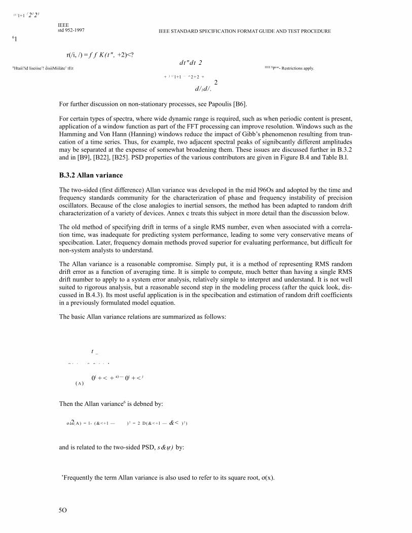
j ( / l + l / 2 t 2 )

61

AHtaíi?iđ liseiỉse1! ểisiiMiiĩáte1 IEE IEEE XP|ore- Restrictions apply.


r(/i, /) = f f K(t" , +2)<?dt"dt 2

+ j ( / l + l — ^ 2 + 2 +

d/ l d/ .2

For further discussion on non-stationary processes, see Papoulis [B6].

For certain types of spectra, where wide dynamic range is required, such as when periodic content is present,application of a window function as part of the FFT processing can improve resolution. Windows such as theHamming and Von Hann (Hanning) windows reduce the impact of Gibb’s phenomenon resulting from trun-cation of a time series. Thus, for example, two adjacent spectral peaks of signibcantly different amplitudesmay be separated at the expense of somewhat broadening them. These issues are discussed further in B.3.2and in [B9], [B22], [B25]. PSD properties of the various contributors are given in Figure B.4 and Table B.l.

B.3.2 Allan variance

The two-sided (first difference) Allan variance was developed in the mid l96Os and adopted by the time andfrequency standards community for the characterization of phase and frequency instability of precisionoscillators. Because of the close analogies to inertial sensors, the method has been adapted to random driftcharacterization of a variety of devices. Annex c treats this subject in more detail than the discussion below.

The old method of specifying drift in terms of a single RMS number, even when associated with a correla-tion time, was inadequate for predicting system performance, leading to some very conservative means ofspecibcation. Later, frequency domain methods proved superior for evaluating performance, but difficult fornon-system analysts to understand.

The Allan variance is a reasonable compromise. Simply put, it is a method of representing RMS randomdrift error as a function of averaging time. It is simple to compute, much better than having a single RMSdrift number to apply to a system error analysis, relatively simple to interpret and understand. It is not wellsuited to rigorous analysis, but a reasonable second step in the modeling process (after the quick look, dis-cussed in B.4.3). Its most useful application is in the specibcation and estimation of random drift coefficientsin a previously formulated model equation.

The basic Allan variance relations are summarized as follows:

t _

0(t ) = f &(t )dt

( A )0( +< + a) — 0( +< )

Then the Allan variance6 is debned by:

ơ & ( A ) = l - ( & < + l — ) 2 = 2 D ( & < + l — &< ) 2 )2

and is related to the two-sided PSD, s&ự) by:

’Frequently the term Allan variance is also used to refer to its square root, ơ(x).

5O

AHtliOír§ld licensed ito E^§l&ft(í9rảSWâfsíỉ§!SlíifelÌ®tffen Kft'WSlỹlldedjSra(?Cị9:l?fttdm?iêẼI0<a,b0ỉ:;P0âfìfclrffi^íÍỄPIỊ' IEEE XP|ore- Restrictions apply.

Stochastic model contributor Asymptotic propertiesPSD Sự)

Nomenclature

Equivalent white noiseinput

other name 0 & S&#

Generic This std

White angle Aĩ 2N0 H2 Angle measurementnoise O +2 (26/ )212

Angle

quantization— Q2 White angle energy

spectrum O +22

' Q . 2 ,

Flicker angle2

N F0— Pink angle noise -1 +1 2 6 / N .0

Angle randomwalk, white ratenoise

2

N&"2 Reg angle noise -2 O "2

Rate

quantization— —

Discrete white ratenoise or white rateenergy spectral density

-2 O —

Bias instability 2 B2 Pink rate noise -3 -1 --B2--

Markov rate2

Nc&B2 Correlated drift rate -2, -4 O, -2

--?CAC-2

1 + (2 6 / AC Ỷ

Rate

randomN 2N & %2 Red rate noise -4 -2

- -%2-

( 26/ )2

Ramp instabil- N 2 &2 Pink angular accelera-tion noise

-5 -3 - -&2-


Std 952-1997

4ơ2

&

There is no inversion formula.

One of the most notable deficiencies of the Standard Allan variance is the non-unique characterization ofwhite anele. Aicker anele. and auantization noiseat the hieh freauencv end. and random rate ramn vs. Aickerangular acceleration at the low-freauencv end. These, however, mav be sorted out bv using the ModidedAllan variance and/or prewhitening methods discussed in B.4.3. Other approaches include applving a prefil-ter to the time series (such as a triangular filter), or alternativelv incorporating it into the Allan variance com-putation, or applving it as a window. The theorv and use of windows is discussed bv Hamming [B22]. Thisapproach is equivalent to some of the other variance methods discussed bv Rutman [B25].

If the standard Allan variance is viewed as an application of a variable rectangular window to the time series,then the Modided Allan variance mav be viewed as the application of a variable triangular window to thetime series. Maximum efficiencv is obtained bv using an algorithm that uses maximum overlap. Some ofthese issues are discussed in Stovall [B39], where a triangular predlter with maximum overlap is suggested.The more obvious advantage of the higher order Altering is in dealing with these high pass processes (thosewith positive PSD slopes) bv terminating the Altered process in a controlled low pass characteristic, insuringa finite variance.

Allan variance properties of the various contributors is given in Table B.l.

Copyright © 1998 IEEE. All rights reserved. 5l


Random bias &( O) B O2 Bias or fixed draft See Note 2 See Note 2 #Oô( / )

Random ramp & (O) &O2 Rate ramp See Note 2 See Note 2 —

Periodic rate &O — HarmonicDiscretespectra

Discretespectra

1 &2ô(/ - / O)

AHtliOíí§id to lAâ^SMSrUnSắiíslíelSíỉMPẾín Pấ?,'wa|ỹiideíbsra(?cịo!?ftfc0?iêẼltXat)0ỉ:;Rìẩ6fclrffi<?ííỄPiỊ' IEEE xp|ore- Restrictions apply.

Asymptotic propertiesAllan variance ơ(t)

0 & Ơ&(a)

-1/2 -1, (-3/2)See!Note!1

3 O2/

2 f nA

NOTES

1 —Mod ơ—Modified Allan variance

52


Std 952-1997

in frequency and tau domain

O -12

3Q

2O -1 "0[3 (2+ln26 f n x) - ln2]

26A

+ 1/2 -1/2"2

A

+ 1 O —

+1 O 2 B2 ln 26

+ 1 1/2, +1/2 + 1/2, -1/2( B C

TC ) 2 \ . * C >3 -1

2 2 A L 2A l3-4e + = JJ

+1!1/2 +1/2K 2 A

3

+2 +1 —

See!Note!2 See Note 2 —

See!Note!2 See Note 222

&O A

2

See!Note!2 See Note 22

^2 sin 6f OA

&O 2

AHtliOíí§id licensed ảỉpemimteí1 to lAâ^SMSrUnSắiíslíelSíỉMPẾín IEEE xp|ore- Restrictions appiy.

NOTES

1 —Mod ơ—Modified Allan variance


53

AHtl»írgld licensed ito E^§!&ft(í9rảSWâfsíỉ§!SlíifelÌ®tffen Kft'WSlỹlldedjSra(?Cị9:l?fttdm?iêẼI0<a,b0ỉ:;P0âfìfclrffi^íÍỄPIỊ' IEEE XP|ore. Restrictions apply.


B.4 Test, data Processing, and analysis considerations

This clause discusses methods of test, data acquisition, and data Processing. Several suggestions are madetoimprove the efficiency of these operations and the subsequent analysis.

B.4.1 Approach

General test conditions and equipment are discussed in Clause 11. Test procedures are discussed in 12.11. Itis important to control the influence of external environments on the test. External sources of error shouldberemoved or compensated for in an appropriate pre-filter. Differential techniques (such as back-to-backsensortest) are also effective. Error detection/correction is also an important step of the data acquisition process.

Sample rates, anti-aliasing Altering, and record lengths are to be chosen with regard to various system con-siderations [B9]. The longer term effects of random drift on performance with regard to the mission profileshould be separated out using signal processing techniques prior to data acquisition, and the higher fre-quency data should be analyzed separately.

B.4.2 Data acquisition

In terms of economy, efficiency is achieved by combining data reduction methods into the data acquisitionprocess [B36] and [B37], thus transforming data into a more usable form. Generally, the sample rate isselected to be at least twice the sample bandwidth (limited by Altering to the highest frequency of interest),however, Papoulis [B6] shows that six samples per bandwidth cycle are required to characterize a signalfromits past values only. The record length should be at least several times the required performance interval, asdictated by the mission profile. Coverase of too larse a temporal dynamic ranse. however. is uneconomical.impractical, and unnecessary; collectins O.1 ms data for 1OOO h yields a laree, unwieldy number of datapoints.

The recommended approach is to limit the time/frequency domain dynamic range (of record length tosampleperiod) to about 3 orders of magnitude. This is done by dividing the total range into overlapping intervals ofgeometrically increasing lengths. Thus, the high frequency data is acquired for a short period of time.Lowerfrequency data is Altered (integrated) and acquired for a longer period (e.g., O.1ms data collected for O.1 s,O.O1 s data for 1O s, 1 s data for 1OOO s and 1OO s data for 1O5 s). Signal processing is used to removetheundesired effects outside the bandwidth of interest. It is noted that frequency domain (PSD) analysis is par-ticularly appropriate to investigating high frequency phenomena as well as long term random drift, whereastime domain analysis should be condned to the low-frequency phenomena where it is often simpler to use.

The appropriate sampling rates/record lengths should be chosen to overlap about one decade of frequency(time), consideration being given to the particular characterization of the process. Prior characterization ofthe process is necessary for proper determination of data acquisition parameters. One approach is to choosegeometric means of the record length and sample period to correspond to the geometric mean of the corre-sponding frequency or time domain range of the dominant characteristic of interest. For example, if biasinstability (flicker) is to be observed in the interval 1ơ ị s to 1O6 s (1.O-1OO mHz) the geometric mean is1O5 s(1O mHz); the corresponding sample period and record length would be ~ 1O%/^ s and ~ 1O%/ĨỠ srespectively. However, if the mission profile provided for a fix (or calibration) at 1O5 s a record length of

)á(/) - "á + -

2

" 2 .VQ

---1

"aE "á E

) R ( / ) — H RQ ( j / ) ) á ( / ) H RQ (

j / ) — | H & á ( ) á ( / )

AHtaíi?iđ ảỉpemimteí1 to lAâlSMSrUnSắiíslíelSíỉMPẾín IEEE xp|ore- Restrictions apply.


Std 952-1997

B.4.3 Post-Processing

Post-processing of the acquired data includes the quick look data editing, trend removal, digital -ltering ofother deterministic signal (i.e., periodic) and other pre-whitening signal Processing.

The quick-look is a cursory visualization of each record of the data in the form of graphical time series. Baddata is edited out and replaced by interpolated or simulated data. Trends are observed for removal and sepa-rate analysis by least squares estimation techniques. Possible periodic content is observed for removal byother -ltering techniques. Such removal is a -rst step in the prewhitening processing.

Best estimates of the model are achieved when the estimation error (residuals, innovations) is a white noiseprocess. Some analysis techniques, such as an adaptive Kalman -lter can be designed to do this. Anotherapproach requires a priori knowledge of the stochastic model [B36] and [B37].

In this approach, an inverse -lter is mechanized in the signal processing to pre-whiten the data (exampleFig-ure B.3). This may simply entail applying either an integration operation (as with angle white noise) or adif-ferencing operation (as with rate random walk). As a practical matter, additional high frequency poles mustbe added to band limit the resulting dynamic range required for subsequent analysis.

H (E) -"& 1 x, "á

+ —--- "á + —

f 2 " á" & + - - &

m

" 2 -

j2 ‘"á

Stocha Prewhitening


55

AHtliOíí§id ảỉpemimteí1 to lAâlSMSrUnSắiíslíelSíỉMPẾín IEEE xp|ore- Restrictions apply.

RAN DOM FIXED DRIFT QUANTIZATIONRAMP (RANDOM NOtSEù(0) BIAS) ANGLE

1 WHITE VVHITE HIGH FREQUENCY

JL NOISE NOISE ACCUMULATOR1 ỈD 0


B.4.4 Time series analysis considerations

Subsequent to data acquisition and post-processing, the resulting processed data records are prepared fortime series analysis. Whichever method is used, time or frequency domain analysis, there are some sug-gested guidelines to follow.

Each data record so constructed contains piece-wise information to be extracted and re-assembled in a com-posite analysis, which will then display the full dynamic range of the desired result. In re-assembling thecomputed information in the appropriate chart, it may be necessary to undo some of the previous operationto put the output data into the proper format and proper units. If, for example, pre-whitening processing wasapplied, the corresponding post-darkening operation will be necessary to reconstruct the characteristic signa-ture of the analyzed data.

Prior to this operation however, the model coefficients are hrst estimated. A hrst approximation (secondapproximation if prewhitening has been performed) can be estimated by sketching in the asymptotes to thecharted data analysis, and computing approximate model coefficients. A prewhitening hlter may be derivedand the error coefficients from the residuals may be reestimated. Alternatively, a more rigorous weightedleast squares procedure, which weights by the inverse error covariance, may be used. Error bounds on thecoefficient should be computed to establish the goodness-of-fit.

With the coefficients thus determined, and the composite data analysis assembled on the appropriate chart,the resulting characteristic curve fit can be superimposed on the charted data, together with the error boundsto give a detailed representation of the stochastic model characterization. The coefficients are also used toconstruct a block diagram (Figure B.4) and generate the detailed state equations describing the stochasticmodel.

B.4.5 Example

Figures B.5 and B.6 illustrate the piecewise asymptotic representation of the Allan variance and correspond-ing PSD of a hypothetical gyro with parameters:

N = O.OO1 °/Jh

B = O.OO1 °/h

K = O.OOO1 °/ h3 7

2

Q = O.577"

angle random walk

bias instability

rate random walk

quantization noise (result of 2"/p gyro scale factor)

Inertial systems design and performance prediction depends on accurate knowledge of sensor level behavior.

This annex has attempted to provide a brief introduction and roadmap to the study of a very extensive sub-ject of dynamic and stochastic modeling as it applies to this purpose.

Through better understanding of the modeling process and standardization of test and reporting of data, theinertial system and gyro designer can more effectively meet their goals.

56

ọ

ò

T3CQ

tac

ro£>

1

ro00?r

Q.0ơ>00ịr

0)

3

ọ

0c

Q.

0)

0)

ũ)0Ì2

c

AHtl»íisid licsnsed ểtíseliiaiíe1 Ito IEEE XP|ore- Restrictions apply.

RRST-ORDER MARKOVPROCESS(CORRELATED RANDOM

IEEE

FORSINGLE-AXISINTERFEROMETRICFIBEROPTICGYROSstd952-1997

(M/o

X1)0

[zH/j(ụ/o)](ifo


A (h)

f (Hz)

58


Std 952-1997

B.6 Chronological bibliography

[Bl] Von Neuman, J., and Morgenstem, o., Theory of Games and Economic Behavior, New York: JohnWiley and Sons, 1967, Princeton University Press, 1944.

[B2] Wiener, N., Cybernetics: or Control and Communication in the Animal and the Machine. Cambridge,MA: MIT Press, 1948, Second Edition 1961.

[B3] Kalman, R. E., “A New Approach to Linear Filtering and Prediction Problems,” ASME Transactions,Vol. 182D, Mar. 1960, pp. 35-45.

[B4] Hannan, E. J., Time Series Analysis. Great Britain: Science Paperbacks and Methuen and Co. LTD,196O, Reprinted 1967.

[B5] Parzen, E., Stochastic Processes. San Francisco, CA: Holden-Day, 1962.

[B6] Papoulis, A., Probability, Random Variables and Stochastic Processes. New York: McGraw-Hill, 1965.

[B7] Machol, R. E., Systems Engineering Handbook. New York: McGraw-Hill, 1965.

[B8] Allan, D. W., “Statistics of Atomic Frequency Standards,” Proceedings of the IEEE, vol. 54, no. 2,pp. 221-230, Feb. 1966.

[B9] Bendat, J. S., and Piersol, A. G., Measurement and Analysis of Random Data. New York: John Wileyand Sons, 1966.

[B10] Gelb, A., and Sutherland, A. A. Jr., “Design of Strapdown Gyroscopes for a Dynamic Environment,”TASC report TR101-1, 1967.

[B11] Sutherland, A. A., and Gelb, A., “Applications of the Kalman Filter to Aided Inertial Systems,”NWC-TP-4652, China Lake, CA, Aug. 1968.

[B12] Van Trees, H. L., .Detection, Estimation, and Modulation Theory, Part I, New York: John Wiley andSons, 1968.

[B13] Wrigley, et al., Gyroscopic Theory, Design, and Instrumentation. Cambridge MA: M.I.T. Press, 1969

[B14] Box, G. E. P., and Jenkins, G. M., Time Series Analysis: Forecasting and Control. San Francisco: :Holden-Day, 1970, Revised 1976.

[B15] Britting, K., Inertial Navigation Systems Analysis. New York: Wiley-Insterscience, 1971.

[B16] Barnes, J. A., et al., “Characterization of Frequency Stability,” IEEE Transactions onInstrumentationand Measurement, vol. IM-20, pp. 105-120, May 1971.

[B17] Coffman, V. “On-Line Estimation of Parameters Using Experimentally Developed Gyro Models, andOther Applications,” Ph.D. diss., Stanford University, SUDAAR no. 467, Dec. 1973.

AHtlìOíí§id Ito ^ẵl&PtíarảSSMSíỉẽtiĩntíầliotPíkn IEEE XP|ore- Restrictions apply.

AHtl»írgld licsnsed ểmMtgd ito E^§!&ft(í9rảSWâfsíỉ§!SlíifelÌ®tffen Kft'WSlỹlldedjSra(?Cị9:l?fttdm?iêẼI0<a,b0ỉ:;P0âfìfclrffi^íÍỄPIỊ' IEEE XP|ore- Restrictions apply.


[B21] Giacoletto, L. J., Electronics Designers’ Handbook, Second Edition. New York: McGraw-Hill,pp.16-20, 1977.

[B22] Hamming, R. w., Digital Filters. Englewood Cliffs, NJ: Prentice Hall, 1977.

[B23] Lindsey, w. C., and Chie, C. M., “Identihcation of Power-Law Type Oscillator Phase Noise Spectrafrom Measurements,” IEEE Transactions on ỉnstrumentation and Measurement, vol. IM-27, no. 1, pp. 46-53, Mar. 1978.

[B24] Sargent, D. and Wyman, B.O., “Least Squares and How They Give Us Fits,” Second Printing, TRWReport 32143-61O1OTU-0o, 9 June 1978.

[B25] Rutman, J., “Characterization of Phase and Frequency Instabilities in Precision Frequency Sources:Fifteen Years of Progress,” Proceedings o/the IEEE, vol. 66, no. 9, Sept. 1978.

[B26] Kochakian, C. R. “Time-Domain Uncertainty Charts (Green Charts): A Tool for Validating theDesignof IMU/Instrument Interfaces,” Proceedings o/ the AIAA Guidance and Control Con/erence, Aug. 11-13,1980.

[B27] Sargent, D. and Wyman, B. O., “Extraction of Stability Statistic from Integrated Rate Data,”Proceed-ings o/the AIAA Guidance and Control Con/erence, Aug. 11-13, 1980.

[B28] Cadzon, J. A., “High Performance Spectral Estimation—A New ARMA Method,” IEEETransactionson Acoustics, Speech, and Signal Processing, vol. ASSP-28, ,o. 5, pp. 524-528, Oct. 1980.

[B29] Allan, D. w., and Barnes, J. A., “A Modihed ‘Allan Variance’ with Increased Oscillator Characteriza-tion Ability,” Proceedings o/ the 35th Annual Frequency Control Symposium, pp. 470-475, May 1981.

[B30] Howe, D. A., et al., “Properties of Signal Sources and Measurement Methods,” Proceedings o/ the35th Annual Frequency Control Symposium, pp. 441-447, May 1981.

[B31] Britting, K., et al., “Statistical Description of Quantization Error”, Northrop, PPD, unpublishedpaper,1982.

[B32] Keshner, M. S., “1/f Noise,” Proceedings o/the IEEE, vol.70, no. 3, pp. 212-218, Mar. 1982.

[B33] Sinha, N. K. and Kuszta, B., Modeling and Identification o/Dynamic Systems, New York: Van Nos-trand Reinhold, 1983.

[B34] Tehrani, M. M., “Ring Laser Gyro Data Analysis with Cluster Sampling Technique,” Proceedings o/SPIE, vol. 412, 1983.

[B35] King, A. D., “Characterization of Gyro In-Run Drift,” Symposium Gyro Technology 1984, pp. 10.0-10.56, Oct° 1984.

[B36] Mark, J. and Brown, A., “Laser Gyroscope Random Walk Determination Using a Fast Filtering Tech-nique,” Symposium Gyro Technology 1984, pp. 9.0-9.21, Oct. 1984.

[B37] Vallot, L., et al., “Short Acceptance Test Procedures for Ring Laser Gyros,” 12th Biennial GuidanceTest Symposium, pp. 1-12, 22-24, Oct. 1985.

[B38] Walls, F. L., and Allan, D. w., “Measurements of Frequency Stability,”Proceedings o/IEEE, vol. 74,no. 1, Jan. 1986.

AHtlìOíí§id ảỉpemimteí1 to lAâlSMSrUnSắiíslíelSíỉMPẾín IEEE xp|ore- Restrictions apply.


Std 952-1997

[B39] Stovall, s. H., “Analysis of Ring Laser Gyro Noise Measurement Techniques,” China Lake CA: NWCTechnical Report, 1987.

[B4O] Allan D., et al., “Standard Terminology for Fundamental Frequency and Time Metrology,” ProposedIEEE Standard Para-P-1139.

[B41] Erickson, G. W., “An overview of Dynamic and Stochastic Modeling of Gyros,” Proceedings of the1993 National Technical Meeting of the lON, Jan. 1993.


61

7This annex is adapted from Annex C in IEEE Std 647-1995, IEEE Standard Specification Format Guide and Test Procedure for

Single-

Axis Laser Gyros.

8The numbers in brackets preceded by the letter C correspond to those of the bibliography in C.4.

9Sometimes referred to as time series or data streams.


Annex c7

(informative)

An overview of the Allan variance method of IFOG noise analysis

c.1 Allan variance backgroundAllan variance is a time domain analysis technique originally developed to study the frequency stability ofoscillators [Cl].8 It can be used to determine the character of the underlying random processes that give riseto the data noise. As such, it helps identify the source of a given noise term in the data. The source may beinherent in the instrument, but in the absence of a plausible mechanism within the instrument its origin shouldbe sought in the test set up. The Allan variance adopted in this standard may be used as a stand-alone methodof data analysis or to complement any of the frequency domain analysis techniques. It should be mentionedthat the technique can be applied to the noise study of any instrument. Its valueA howeverA depends upon thedegree of understanding of the physics of the instrument. Following is an overview of the Allan variance andits adaptation to the noise properties of IFOGs, similar to that described in [C6] for ring laser gyros.

In the Allan variance method of data analysis, the uncertainty in the data is assumed to be generated by noisesources of specihc character. The magnitude of each noise source covariance is then estimated from the data.The dehnition of the Allan variance and a discussion of its use in frequency and time metrology is presentedin [Cl] and [C7].

In this annex, Allan’s dehnition and results are related to five basic gyro noise terms and are expressed in anotation appropriate for gyro data reduction. The five basic noise terms are angle random walk, rate randomwalk, bias instability, quantization noise, and rate ramp.

Consider N samples of gyro data9 with a sample time of A0. Form data clusters of lengths A0, 2Tq, ..., k ĩ Q

0( t ) = C ‘ & ( t ' ) d t

The lower integration limit is not speci-ed as only angle differences are employed in the de-nitions. Anglemeasurements are made at discrete times given by t = kr0, k = l, 2, 3, ..., N. Accordingly, the notation is sim-plihed by writing 0< = 0(kro).

The average rate between times t < and t < + A is given by:

G _ G

r\ í_\ Gk + m Gk

where

A = mx0

62 Copyright © 1998 IEEE. All rightsreserved.

ItRenễedi usmMed ito IEEE Xplore- Restrictions app!y-

Jo (6/A)2

AHtl»íisid ảỉpemimteí1 IEE ^ẵl&PtíarảSSMSíỉẽtiĩntíầliotPíkn IEEE XP|ore- Restrictions apply.


Std 952-1997

The Allan variance10 is dehned as:

ơ2(A) = 1 <(&< + m - &k)2)

= -"2 <(e< + 2:-2G< + m + e< )2)

2A2

where

< ) is the ensemble average

The Allan variance is estimated as

follows: ĩ - 2 mơ (A) =

2A2(N -2:)5 (e < + 2m2e<+ m + e<)

The Allan variance obtained by performing the prescribed operations, is related to the PSD of the noiseterms in the original data set. The relationship between Allan variance and the two2sided PSD11, s&(/) isgiven by:

ơ2 (A) = s&( /) (C.1)Equation (C.1) is the key result that will be used to calculate the Allan variance from the rate noise PSD. Aninterpretation is that the Allan variance is proportional to the total noise power of the gyro rate output whenpassed through a hlter with the transfer function of the form sin4(?)/(?)2. This particular transfer function isthe result of the method used to create and operate on the clusters.

It is seen from Equation (C.1) and the above interpretation that the hlter bandpass depends on A. This sug2gests that different types of random processes can be examined by adjusting the hlter bandpass, namely byvarying A. Thus, the Allan variance provides a means of identifying and quantifying various noise termsthatexist in the data. It is normally plotted as the square root of the Allan variance versus A, [ơ(x)], on a log2logplot.

Subclauses C.1.1 through C.1.7 show the application of Equation (C.1) to a number of noise terms that areeither known to exist in the IFOG or otherwise inhuence its data. Detailed derivations are given in [C6].Thephysical origin of each noise source term will be discussed.

10 Frequently the term Allan variance is also used to refer to its square root, ơ(A).

11 Unless specihcally stated, the term PSD is Annex C refers to the two2sided PSD. Note that s&(/) is thePSD of stationary random

l2The zero slop portion of the rate PSD in (#/h)2/Hz represents angle random walk. The relationship between angle random walk coef-

ficient N and the PSD is

N *•i J i ) = 60M (íÃHz]

AHtliOíí§id Ito ^ẵl&PtíarảSSMSíỉẽtiĩntíầliotPíkn IEEE XP|ore- Restrictions apply.


c.1.1 Angle random walk

The main source for this error is spontaneous emission of photons. This component of the IFOG angle ran-dom walk is caused by the spontaneously emitted photons that are always present in the source output. Theangle random walk due to spontaneously emitted photons is called the quantum limit [C4].

Other high frequency noise terms that have correlation time much shorter than the sample time, can alsocontribute to the gyro angle random walk. However, most of these sources can be eliminated by design.These noise terms are all characterized by a white noise spectrum on the gyro rate output.

The associated rate noise PSD is represented by:

sa( f ) = — (C.2)

where

N is the angle random walk coefficient12

Substitution of Equation (C.2) in Equation (C.l) and performing the integration yields:

A

Figure c.1—Ơ(A) Plot for angle random walk

f > f O

Slope = 0

l i ............. H

: : /<ề

-------------1 -----1 — 1 1 1 I I l i

i -----------1 -----1 1 1 í 1

I I i

1 ----------1- - -1--1 1 11 1 1

AAtiM[zed( tesedUẳusGmiimted teẺ (S9ia(?Eằc0eroỌrPiiẽiickaio^: IEEE Xplore- Restrictions app|y-


Std 952-1997

c.1.2 Bias instability

s0( f )> -? 1

: 2 K ) fO

f4 f O (C.4)

where

B is the bias instability coefficientf O is the cutoff frequency

Substitution of Equation (C.4) in Equation (C.l) and performing the integration yields:

2, ,2 B 2

% (A) = -—-6 ln2 -

• 3

sin X(sinX + 4XcosX) + C ỉ ( 2X) - C ỉ ( 4X) (C.5)

where

X is 6/OA

C ỉ is the cosine-integral function fC2]

Figure C.2 represents a log-log plot of Equation (C.5) that shows that the Allan variance for bias instabilityreaches a plateau for A much longer than the inverse cut off frequency. Thus, the flat region of the plot canbeexamined to estimate the limit of the bias instability as well as the cutoff frequency of the underlying Aickernoise.

1B

0.1B

0.01 B0.01 0.1 10

Figure c.2—Ơ(T) Plot for bias instability (for f0 = 1)


65

ơ(x) = v

AHtl»íisid ảỉpemimteí1 Ito ^ẵl&PtíarảSSâtsíỉẽtiĩntíầliotPíkn IEEE XP|ore- Restrictions apply.


c.1.3 Rate random walk

where

(C.6)

K is the rate random walk

Substitution of Equation (C.6) in

2, , K A

coefficient

Equation (C.l) and performing the integration yields:

(C.7)

This indicates that rate random walk is represented by a slope of +l/2 on a log-log plot of ơ(x) versus A, asshown in Figure C.3. The magnitude of this noise can be read off the slope line at A = 3.

A

Figure c.3—ơ(x) Plot for rate random walk

c.1.4 Rate ramp

For long, but finite time intervals this is more of a deterministic error rather than a random noise. Itspresencein the data may indicate a very slow monotonic change of the IFOG source intensity persisting over a longperiod of time. It could also be due to a very small acceleration of the platform in the same direction andper-sisting over a long period of time. It appears as a genuine input to the IFOG given by:

/ S 2Xo

AHtl»íisid ảỉpemimteí1 IEE ^ẵl&PtíarảSSMSíỉẽtiĩntíầliotPíkn Pấ?,'wa|ỹiideíbsra(?cịo!?ftrc0?iêẼltXat)0ỉ:;Rìẩ6fclrffi<?ííỄPiỊ' IEEE XP|ore- Restrictions apply.


Std 952-1997

By forming and operating on the clusters of data containing an input given by Equation (C.8), we obtain:

&2 2ơ2(X) = RA- (C.9)

This indicates that the rate ramp noise has a slope of +1 in the log-log plot of ơ(x) versus X, as shown in

Fig-

ure C.4. The magnitude of rate ramp R can be obtained from the slope line at X = J2 .The rate PSD associated with this noise is:

)&(/)=R 2

(26/)3

(C.1O)

The user should be aware that there may be a flicker acceleration noise with 1I/3 PSD that leads to the sameAllan variance X dependence. See Annex B for a discussion.

X

Figure C.4—ơ(x) plot for rate ramp

c.1.5 Quantization noise

)0( /) =

sin (6/X0)N

(6/AO)2 ;

“X O '

XO(C.11)

where

is the quantization noise coef-cient


67

X0

AHtl»íisid liseiỉse1! ểisiiMiiĩáte1 IEE IEEE XP|ore- Restrictions apply.

(1)0


The theoretical limit for Q is equal to s/ Jĩ2 where s is the gyro scale factor, for tests with hxed and uni-form sampling times. The rate PSD is related to the angle PSD through the equation:

s&( 26/) = (26/ )2se( 26/) (C.12)

and is

s&(/) =

4Q2 . 2--f-sin (6/A0)R(26/)2A0QQ / < 2-

2x0 (C.13)

Substitution of Equation (C.13) in Equation (C.1) and performing the integration yields:

2

ơ2(x) = 3Q (C.14)

X

This indicates that the quantization noise is represented by a slope of -1 in a log-log plot of ơ(x) versus X, as

shown in Figure C.5. The magnitude of this noise can be read off the slope line at X = J3 .

The user should be aware that there are other noise terms with different spectral characteristics, such asflicker angle noise and white angle noise, that lead to the same Allan variance X dependence. See Annex Bfor a discussion of these noise terms.

X

Figure C.5—ơ(x) Plot for quantization noise

68

where

&O is the amplitude

Ẩ) is the frequency

ô(?) is the Dirac delta function

AHtaíi?iđ tensedi ảỉpemimteí1 IEE ^ẵl&PtíarảSSMSíỉẽtiĩntíầliotPíkn IEEE xp|ore- Restrictions apply.


Std 952-1997

c.1.6 Other noise terms

c.1.6.1 Exponentially correlated (Markov) noise

This noise is characterized by an exponential decaying function with a finite correlation time.

The rate PSD for such a process:

)&(/) = - (C.15)

1 + (2 6 / T C )2

where

q C is the noise amplitude

T C is the correlation time

2, , _ (q—cYơ (%) = _

T_CL>

% 2% (C.16)

Figure C.6 shows a log-log plot of Equation (C.16). It is instructive to examine various limits of this equa-tion. For % much longer than the correlation time, it is found that:

ơ2(%) T (^q—C-Ị- % » T C (C.17)

which is the Allan variance for angle random walk where N = q C T C is the angle random walk coefficient. For% much smaller than the correlation time, Equation (C.16) reduces to:

q2

ơ2(%) T qQ-% % « T C (C.18)

which is the Allan variance for rate random walk.

c.1.6.2 Sinusoidal noiseThe PSD of this noise is characterized by one or more distinct frequencies. A low-frequency source could bethe slow motion of the test platform due to periodic environmental changes. A representation of the PSD ofthis noise containing a single frequency is given as:

12

) & ( / ) = 2&O[8( / - /O) + ô( / + /O)] (C.19)

AHtliOír§ld licsnsed ảỉpemimteí1 to E^§l&ft(í9rảSWâfsíỉ§!SlíifelÌ®tffen Kft'WSlỹlldedjSra(?Cị9:l?ftfdm?iêẼI0<a,b0ỉ:;P0âfìfclrffi^íÍỄPIỊ' IEEE XP|ore- Restrictions apply.


Multiple frequency sinusoidal errors can be similarly represented by a sum of terms such as Equation (C.19)at their respective frequencies and amplitudes. Substitution of Equation (C.19) in Equation (C.1) and per-forming the integration yields:

ơ2 (A) = &O sin26 / O

A?6 OA ;

(C.2O)

Figure C.7 shows a log-log plot of Equation (C.2O). Identibcation and estimation of this noise in IFOG datarequires the observation of several peaks. As is seen however, the amplitudes of consecutive peaks fall offrapidly and may be masked by higher order peaks of other frequencies making observation difficult.

0.01 0.1 1 10

A f0

Figure C.7—Ơ(A) Plot for sinusoidal error

7O

ơtot (A) = ƠARW(a) h ơquant(A + h %BiasInst(A) h ... (C.21)


Allan [Cl](rate domain)

This Standard(rate!domain)

Sargent, Wyman [C3](angle domain)

Tehrani [C6](rate domain)

Terms invarianceexpressionfor noiseprocesses

A = samplingtime = mro

whereAo = sampletime of originalmeasurements

1/*O = datasample raten = 1, 2, 3,...

V = time interval separatingraw data points(2L+1) = number of datapoints combined into anaverage data pointA = time length of data span =(2L+1)ynn = 1, 2, 3,...

Q =

TC = correla-tion timeT = clustertime

v0 = cutofftrequency for

Rate ramp Not addressedR2

■(nTo-2]

2R 2 [T4] R

2[ T2 ]


Std 952-1997

c.1.7 Combined effects of all processes

In general, any number of the random processes discussed above (as well as others) can be present in thedata. Thus, a typical Allan variance plot looks like the one shown in Figure C.8. Experience shows that inmost cases, different noise terms appear in different regions of A. This allows easy identihcation of variousrandom processes that exist in the data. If it can be assumed that the existing random processes are allstatis-tically independent then it can be shown that the Allan variance at any given A is the sum of Allan variancesdue to the individual random processes at the same A. In other words,

Thus estimating the amplitude of a given random noise in any region of A requires a knowledge of theampli-tudes of the other random noises in the same region.

C.2 Estimation accuracy and test design

A -nite number of clusters can be generated from any -nite set of data. Allan variance of any noise term isesti-mated using the total number of clusters of a given length that can be created. Estimation accuracy of theAllanvariance for a given A, on the other hand, depends on the number of independent clusters within the dataset.

ơ= (C.22)

Equation (C.22) shows that the estimation errors in the regions of short (long) A are small (large) as thenum-ber of independent clusters in these regions is large (small). In fact, this equation can be used to design atestto observe a particular noise of certain characteristics to within a given accuracy. For example, to verify theexistence of a random process with a characteristic time of 24 h in the data to within an error of 25%. We


Kmax = P (C.23)

Since the suspected characteristic time is 24 h, clusters of the same length are created. Thus the total testlength needed for such a test is 24 X 9 = 216 h.

C.3 Tabulation of some variance analyses

A summary comparison of some variance analyses for noise processes is made in Table C.1. This table pre-sents only a sample of analyses available, and is not meant to be a survey of all analyses. The polynomialvariance terms in the left hand column are identihed using gyro terminology. The individual terms relatingtoeach author’s publication are given with the same symbology as contained in that author’s publication,including the dehnitions of symbols. For ease in recognition of similarities, the coef-cients of interest are

Table C.1—Summary comparison of publishing variance analyses for noise processes

Rate randomwalk

h-.pí-] % 4T]

K 2

^T3 2 L * L + 1 ) V 2 A3 3 +

L ( L + 1) ( 12 L2 + 12 L + 1 )V 3

L 15( 2 L + 1) J

2-2*1q ư J

for T 4 TO

Bias

instability

hp1[ 2ln2 ] B^6ln2] Analysis considers only time-dependent rate terms #DH

for T » -1

v0

Angle

random walkh-[fj

Ơ2|~2T -'V^+^I

L 2L +1 JQU]

Quantization

noise

Not addressedLư H 2 \

6 1Not addressed

AHtlìOíí§id ảỉpemimteí1 Ito ^ẵl&PtíarảSSMSíỉẽtiĩntíầliotPíkn IEEE xp|ore- Restrictions apply.

72


13IEEE Std 1139-1988 has been withdrawn; however, copies can be obtained from Global Engineering, 15 Inverness Way East, Engle-

wood, CO 80112-5704, USA, tel. (303) 792-2181.

AHtlì0íí§id ảỉpemimteí1 Ito ^ẵl&PtíarảSSâisíỉẽtiĩntíầliotPíkn Pío'wa|ỹiideíbsra(?cịo!?ftic0?iêẼltXat)0ỉ:;Rìẩ6fclrffi<?ííỄPiỊ' IEEE XP|ore. Restrictions apply.


Std 952-1997

C.4 Bibliography for Annex c

[Cl] Allan, D. w., “Statistics of Atomic Frequency Standards,” Proceedings of the IEEE, vol. 54, no. 2,pp. 221-230, Feb 1966.

[C2] Gradshteyn, I. S. and Ryzhik, I. M., Table of Integrals, Series, and Products. Academic Press, 1980.

[C3] Sargent, D., and Wyman, B. o., “Extraction of Stability Statistic from Integrated Rate Data,” Proceed-ings of the AIAA Guidance and Control Conference, Aug. 11-13, 1980.

[C4] Simpson, J. H., Proc. NAECON, vol. 1, p. 80, 1980.

[C5] Keshner, M. S., “1/f Noise,” Proceedings of the IEEE, vol. 70, no. 3, pp. 212-218, Mar. 1982.

[C6] Tehrani, M. M., “Ring Laser Gyro Data Analysis with Cluster Sampling Technique,” Proceedings ofSPIE, vol. 412, 1983.

[C7] IEEE Std 1139-1988, IEEE Standard Definitions of Physical Quantities for Fundamental Frequencyand Time Metrology.13


73

Clause 5 # Clause 5 requirement Clause 6 # Clause 6.6 test method

5 Requirements N/T

5.1 Description N/T

5.2 General requirements N/T

5.2.1 Precedence N/T

5.3 Performance N/T

5.3.1 Input Rate limits 6.6.1O Input rate test series

5.3.1.1 Maximum 6.6.1O.1 Maximum input rate

5.3.1.2 Minimum (dead band) 6.6.1O.2 Minimum input rate

5.3.2 Gyro scale factor, s 6.6.9.1 Gyro scale factor

5.3.2.1 Gyro scale factor errors 6.6.9.2 Gyro scale factor errors

5.3.2.2 Gyro scale factor sensitivities 6.6.9.3 Gyro scale factor sensitivities

5.3.3 Drift rate, D, E 6.6.11 Drift rate test series

5.3.3.1 Bias and random, D 6.6.11 Drift rate test series

5.3.3.1.1 Bias, Dp 6.6.11.1 Bias

5.3.3.1.2 Random, D& 6.6.11.3 Random drift

5.3.3.1.3 Measurement noise, DQ 6.6.11.2 Measurement noise

5.3.3.2 Environmentally sensitive, E 6.6.11.1 Bias

5.3.3.2.1 Thermal 6.6.11.1 Bias

5.3.3.2.2 Magnetic 6.6.11.1 Bias

5.3.3.2.3 Other sensitivities 6.6.11.1 Bias

5.3.4 IA alignment characteristics 6.6.12 IA alignment test series

5.3.4.1 IA misalignment 6.6.12.1 Misalignment (nominal)

5.3.4.2 IA alignment repeatability 6.6.12.2 Misalignment repeatability

5.3.4.3 IA alignment sensitivities 6.6.12.3 Alignment sensitivities

AHtlìOíí§id licsnsed ảỉpemimteí1 to lAâ^SMSrUnSắiíslíelSíỉMPẾín Pấ?,'wa|ỹiideíbsra(?cịo!?ftfc0?iêẼltXat)0ỉ:;Rìẩ6fclrffi<?ííỄPiỊ' IEEE xp|ore- Restrictions appiy.


Annex D

(informative)

Compliance matrix


5.3.5 Operating temperature 6.6.8.2 Operating temperature

5.3.6 Warm-up time 6.6.6 Warm-up time

5.3.7 Turn-on time 6.6.5 Turn-on time

5.3.8 Polarities 6.6.7 Polarity

5.3.8.1 IA 6.6.7 Polarity

5.3.8.2 Output signals 6.6.7 Polarity

5.3.9 Reference constants N/T

5.3.9.1 Light source wavelength N/T

5.3.9.2 Number of turns N/T

5.3.9.3 Effective area per turn N/T

5.3.9.4 Physical pathlength N/T

5.4 Mechanical requirements 6.6.1Examination of product(mechanical)

5.4.1 Exterior surface6.6.1

Examination of product(mechanical)

5.4.2 Outline and mounting dimen-sions 6.6.1

Examination of product(mechanical)

5.4.3 Gyro axes 6.6.1Examination of product(mechanical)

5.4.4 Weight 6.6.1Examination of product(mechanical)

5.4.5 Seal 6.6.3 Leak test

5.4.6 Identification of product 6.6.1Examination of product(mechanical)

5.4.7 Acoustic noise 6.6.13.2 Acoustic noise

5.5 Electrical requirements 6.6.2Examination of product(electrical)

5.5.1 Schematic N/T

5.5.2 Impedances 6.6.2.2 Impedances

5.5.3 Input power 6.6.4 Input power

5.5.4 Test points N/T

5.5.5 Grounding N/T

AHtliOíí§id ảỉpemimteí1 to lAâ^SMSrUnSắiíslíelSíỉMPẾín Pấ?,'wa|ỹiideíbsra(?cịo!?ftfc0?iêẼltXat)0ỉ:;Rìẩ6iblrffi<?ííỄPiỊ' IEEE xp|ore- Restrictions appiy.


Std 952-1997


5.5.6 Output signals 6.6.2,6.6.1O

Examination of product (electrical),Input rate test series

5.5.7 Temperature sensors 6.6.8.1 Temperature sensor characteristics

5.5.8 Insulation resistance 6.6.2.1 Insulation resistance

5.5.9 Dielectric strength 6.6.2.3 Dielectric strength

5.5.1O Electromagnetic interference 6.6.13.1 Electromagnetic interference

5.5.11 Electromagnetic compatibility 6.6.14.17 Electromagnetic fields

5.6 Environmental requirements N/T

5.6.1 Storage 6.6.14 Environmental test series

5.6.2 Transport 6.6.14 Environmental test series

5.6.3 Operation 6.6.14 Environmental test series

5.6.3.1 Operating environment 6.6.14 Environmental test series

5.6.3.2 Survival environment, operating


5.6.3.3 Survival environment, nonoper-ating


5.6.4 Environments N/T

5.6.4.1 Vibration 6.6.14.5 Vibration

5.6.4.1.1 Linear 6.6.14.5.1 Linear

5.6.4.1.2 Angular 6.6.14.5.2 Angular

5.6.4.2 Mechanical shock 6.6.14.3 Mechanical shock

5.6.4.3 Acceleration 6.6.14.6 Acceleration

5.6.4.3.1 Linear acceleration 6.6.14.6.1 Linear acceleration

5.6.4.3.2 Angular acceleration 6.6.14.6.2 Angular acceleration

5.6.4.4 Temperature 6.6.14.1 Temperature

5.6.4.5 Thermal shock 6.6.14.4 Thermal shock

5.6.4.6 Time-dependent temperaturegradient 6.6.11.1

Bias

5.6.4.7 Thermal radiation 6.6.14.12 Thermal radiation

5.6.48 Ambient air pressure 6.6.14.15 Pressure

5.6.49 Acoustic noise 6.6.14.11 Acoustic noise

AHtlìOíí§id licensed ảỉpemimteí1 to lAâ^SMSrUnSắiíslíelSíỉMPẾín Pấ?,'wa|ỹiideíbsra(?cịo!?ftfc0?iêẼltXat)0ỉ:;Rìẩ6fclrffi<?ííỄPiỊ' IEEE xp|ore- Restrictions appiy.



5.6.4.1O Humidity 6.6.14.9 Humidity

5.6.4.11 Air currents 6.6.14.13 Air currents

5.6.4.12 Fungus 6.6.14.8 Fungus

5.6.4.13 Salt spray 6.6.14.1O Salt spray

5.6.4.14 Nuclear radiation 6.6.14.14 Nuclear radiation

5.6.4.15 Magnetic fields 6.6.14.16 Magnetic fields

5.6.4.16 Electromagnetic fields 6.6.14.17 Electromagnetic fields

5.6.4.17 Sand and dust 6.6.14.18 Sand and dust

5.6.4.18 Solar radiation 6.6.14.19 Solar radiation

5.6.4.19 Rain 6.6.14.2O Rain

5.6.4.2O Excitation variation 6.6.14.2 Excitation variation

5.6.4.21 Life 6.6.14.7 Life

5.6.4.21.1 Storage 6.6.14.7.1 Storage

5.6.4.21.2 Operating 6.6.14.7.2 Operating

5.6.4.21.3 Start cycles 6.6.14.7.3 Start cycles

5.7 Reliability N/T

5.7.1 Reliability program N/T

5.7.2 Mean time between failure(MTBF)

6.4.2 Demonstration testing

AHtlìOíí§id ảỉpemimteí1 to lAâ^SMSrUnSắiíslíelSíỉMPẾín Pấ?,'wa|ỹiideíbsra(?cịo!?ftfc0?iêẼltXat)0ỉ:;Rìẩ6iblrffi<?ííỄPiỊ' IEEE xp|ore- Restrictions appiy.


Std 952-1997


77

allan variance ieee

Documents