allen brain observatory overview

OCTOBER 2018 v. 4 alleninstitute.org

Allen Brain Observatory – Visual Coding: Overview brain-map.org

of 26

Allen Brain Observatory

TECHNICAL WHITE PAPER: OVERVIEW

The Allen Brain Observatory presents a comprehensive physiological survey of neural activity in the visual

cortex during sensory stimulation and behavior. This project systematically measured visual responses from

neurons across cortical areas and layers utilizing transgenic Cre lines to drive expression of genetically encoded

fluorescent calcium sensors (GCaMP6). This dataset provides a resource for exploring the progressive coding

of sensory stimuli through the cortical visual pathway at both the single cell and population level.

Figure 1. Schematic of the Allen Brain Observatory data acquisition workflow. Mice expressing genetically encoded calcium sensors in subsets of cortical neurons received implantation of a custom headframe. Intrinsic signal imaging was used to map functional visual areas and retinotopy. Mice were habituated to the passive sensing task. In vivo two-photon calcium imaging was collected across multiple sessions during a diverse set of stimuli. Eye tracking, body position and running data was collected. A surgery monitoring step was performed prior to brain specimen preparation, and anatomical fiducials were aligned by whole-brain serial imaging.

The data acquisition and processing pipeline utilized standardized operating procedures, custom

instrumentation and workflows conducive to scaling. Functionally-defined visual areas were targeted for study

via intrinsic signal imaging (ISI) and single neuron response properties measured by in vivo two-photon calcium

imaging (Fig. 1) in response to a battery of visual stimuli (see “Stimulus Set and Response Analysis” whitepaper

in Documentation). Furthermore, to support community access for analysis of neurophysiology data, the Allen

Institute has served as a founding scientific partner in the effort to develop Neurodata Without Borders (NWB;

http://help.brain-map.org/display/observatory/Documentation

TECHNICAL WHITE PAPER



page 2 of 26

Teeters et al., 2015), a unified data format for cellular-based neurophysiology data. Data in the Allen Brain

Observatory are available in this standardized data format.

This document provides an overview of data acquisition, data processing and quality control procedures used

for this resource. All experimental work described in this paper was performed with approval and oversight of

the Allen Institute Institutional Animal Care and Use Committee. The Allen Institute holds an Animal Welfare

Assurance with the Public Health Service (PHS), and complies with all applicable aspects of the PHS Policy on

Humane Care of Laboratory Animals and the Guide for the Care and Use of Laboratory Animals.

SURGERY

Headframe and Cross-Platform Registration

To enable data acquisition by intrinsic signal imaging (ISI) and two-photon calcium imaging, each animal was

implanted with a stereotaxically-aligned headframe that provides a cranial window for brain imaging and permits

head fixation in a reproducible configuration for repeat imaging of the same brain areas or cells. An integrated

suite of tools (imaging instruments, mouse behavior platforms and implant alignment hardware) was developed

to enable the identical presentation of stimuli across different instruments, and to register data acquired from

different instruments. All measurements are referenced to a plane passing through lambda and bregma and the

mediolateral axis (origin at lambda). Initial measurements showed that the cranial window angle was at 23

degrees of roll, and 6 degrees of pitch. To achieve standardization, a head-frame implant (Fig. 2) was designed

to provide registration relative to lambda and to enable head-fixation at a controlled angle. Use of a custom

fixture enabled placement of the head-frame such that the craniotomy could be repeatability centered at x = -

2.8 mm and y = 1.3 mm on the reference plane.

Figure 2. Headframe for cross-platform registration. Head-frame (A) and head-frame clamp (B). A printed head-plate was made from an acrylic photopolymer [the white part in (A) but produced in a black material] with a well to facilitate the use of liquid immersion objectives. The cranial window was centered within the circular opening. The head-plate slots were used for insertion of Metabond cement. A 304 stainless steel clamp-plate [gray part in (A)] mates with the head-plate and provided durable reference surfaces for subsequent clamping in the instruments. Head-frames were assembled in a jig to ensure uniform offset between the center of the well and the reference surfaces of the clamp, and joined with Loctite 406. The head-frame was mounted in a clamp (B) and registered against the shaft of the shoulder-bolt (center) and the back face of the clamp by the flat-head screw (right) which acts as a wedge. The shoulder-bolt and tertiary clamp bolt (left) were tightened to finalize installation and constrain the clamp-plate against the large flat registration surface of the clamp. Instruments were calibrated using a head-frame that contained a reticle at the nominal center position of the cranial window.

Cranial Window Surgery

Transgenic mice expressing GCaMP6 (see “Transgenic Line Catalog” white paper in Documentation) were

weaned and genotyped at ~p21, and surgery was performed between p37 and p63. Eligibility criteria included:

1) weight ≥19.5g (males) or ≥16.7g (females); 2) normal behavior and activity; and 3) healthy appearance and

posture. Pre-operative injections of dexamethasone (3.2 mg/kg, S.C.) were administered at 12h and 3h before

surgery. Mice were initially anesthetized with 5% isoflurane (1-3 min) and placed in a stereotaxic frame (Model#

1900, Kopf, Tujunga, CA), and isoflurane levels were maintained at 1.5-2.5% for surgery. An incision was made

to remove skin, and the exposed skull was levelled with respect to pitch (bregma-lamda level), roll and yaw.





page 3 of 26

The stereotax was calibrated to lambda using a custom headframe holder equipped with a stylus affixed to a

clamp-plate. The stylus was then replaced with the headframe to center the headframe well at 3.1mm lateral

and 1.3mm anterior to lambda. The headframe was affixed to the skull with white Metabond and once dried,

the mouse was placed in a custom clamp to position the skull at a rotated angle of 20º, such that visual cortex

was horizontal to facilitate creation of the craniotomy. A circular piece of skull 5 mm in diameter was removed,

and a durotomy was performed. A coverslip stack (two 5mm and one 7mm glass coverslip adhered together)

was cemented in place with Vetbond (Goldey et al., 2014). Metabond cement was applied around the cranial

window inside the well to secure the glass window.

Post-surgical brain health was documented using a custom photo-documentation system to acquire a spatially

registered image of the cranial window. One, two, and seven days following surgery, animals were assessed

for overall health (bright, alert and responsive), cranial window clarity and brain health. Brain health is later

assessed by evaluation of 2 photon serial tomography of the brain for abnormalities that could be related to

infection or inflammation. After observing occasional brain health issues in older mice, a series of antibiotic

injections (Ceftriaxone, 175-200 mg/kg, subcutaneous delivery) were added as standard treatment, applied

once a day for three days starting at P80, P110 and P140.

Motion in the headframe was assessed prior to imaging. A trained observer assessed the motion of the

headframe and brain during bouts of running to determine suitability for imaging, by viewing the headframe

under a Leica M80 microscope. If excessive motion was observed during this assessment or at any time during

imaging, mice received a second procedure to apply additional Metabond to the plastic portion of the

headframe—both around the outer edge of the well and at the interface with the metal clamp plate.

INTRINSIC SIGNAL IMAGING (ISI)

Intrinsic signal imaging (ISI) measures the hemodynamic response of the cortex to visual stimulation across the

entire field of view. This retinotopic map effectively represents the spatial relationship of the visual field (or in

this case, coordinate position on the stimulus monitor) to locations within each cortical area. Retinotopic

mapping was used to delineate functionally defined visual area boundaries, and enable targeting of the in vivo

two-photon calcium imaging to retinotopically defined locations in primary and secondary visual areas.

ISI Data Acquisition

Animal preparation. Mice were lightly anesthetized with 1-1.4% isoflurane administered with a somnosuite

(model #715; Kent Scientific, CON) at a flow rate of 100 ml/min supplemented with ~95% O2 concentrated air

(Pureline OC4000; Scivena Scientific, OR). Vital signs were monitored with a Physiosuite (model # PS-MSTAT-

RT; Kent Scientific). Eye drops (Lacri-Lube Lubricant Eye Ointment; Refresh) were applied to maintain hydration

and clarity of eye during anesthesia. Mice were placed on a lab jack platform and headfixed for imaging normal

to the cranial window. The head frame and clamping mechanism ensured consistent and accurate positioning

of the mouse eye in relation to the stimulus screen from experiment to experiment.

Image Acquisition System. To map the retinotopic organization of the cortex and standardize data acquisition,

an ISI system coupled to visual stimulation was assembled. The brain surface was illuminated with a ring of

sequential and independent LED lights, with green (peak λ=527nm; FWHM=50nm; Cree Inc., C503B-GCN-

CY0C0791) and red spectra (peak λ=635nm and FWHM of 20nm; Avago Technologies, HLMP-EG08-Y2000)

mounted on the optical lens. A pair of Nikon lenses operated front-to-front with a back lens (Nikon Nikkor 105mm

f/2.8), and a front lens (Nikon Nikkor 35mm f/1.4), provided 3.0x magnification (M=105/35). The back focal plane

of the 50mm lens was adjacent and coplanar to the cranial window (working distance, 46.5mm), and was

equipped with a bandpass filter (Semrock; FF01-630/92nm) to selectively allow longer wavelengths of reflected

light to reach the camera sensor and to filter screen contamination and ambient light. Illumination and image

time series acquisition were controlled with custom software written in Python. An Andor Zyla 5.5 10tap sCMOS

camera was used at a frame rate of 40Hz with frame intervals timed using the camera’s hardware clock running

at 40MHz. Initiation of simultaneous image acquisition and visual stimulus display was hardware-triggered from

a National Instruments Digital IO board. Acquired images were 2560x2160 pixel/frame, with 16-bit dynamic




page 4 of 26

range and were saved to disk at a 4x4 spatial binning and 4x temporal binning, resulting in 640x640

pixels/frame, 10Hz time series, 32-bit dynamic range and a resulting effective pixel size of 10µm.

Figure 3. Visual stimulus screen placement and presentation. A) Side view of the experimental set up showing the center of the monitor positioned at 10cm away from the eye of the mouse. The monitor was also tilted 70° to the horizontal to present the stimulus parallel to the retina. B) Aerial view of the position of the stimulus monitor showing the screen positioned 30° from the mouse dorsoventral axis also contributing to the parallel relationship between the retina and stimulus display. C) Example snapshot of the stimulus presented, here showing a horizontal sweep moving downwards.

Visual Stimulus for ISI. The lambda-bregma axis of the skull, as positioned in the head frame clamp, was

oriented with a 30° pitch relative to horizontal, corresponding to a horizontal eye position ~60° lateral to midline

and a vertical position ~20° above the horizon (Oommen & Stahl, 2008). To ensure maximal coverage of the

field of view, a 24” monitor was positioned 10 cm from the right eye. The monitor was rotated 30° relative to the

animal’s dorsoventral axis and tilted 70° off the horizon to ensure that the stimulus was perpendicular to the

optic axis of the eye (Fig. 3A, B). The visual stimulus displayed was comprised of a drifting bar containing a

checkerboard pattern, alternating black and white as it sweeps along a gray background (Fig. 3C). The stimulus

bar sweeps across the four cardinal axes 10 times in each direction at a rate of 0.1 Hz (Kalatsky and Stryker,

2003). The drifting bar measures 20° by 155°, with individual square sizes measuring at 25º. The stimulus was

warped spatially so that a spherical representation could be displayed on a flat monitor (Marshel et al., 2011).

Figure 4. Images and maps generated from an individual time series images during an ISI session. A) Image of the vasculature at focal plane, and B) defocused image were used as fiduciary markers to provide cortical reference. For each trial, consisting of 10 sweeps of the drifting bar in the four cardinal directions, five maps were computed: azimuth (C) and altitude (D) maps, amplitude maps of the signal




page 5 of 26

intensity for both vertical and horizontal sweeps (not shown), and a sign map. The sine of the angle between the horizontal and vertical map gradients was used to generate the sign map (E). Scale bar in degrees for C & D.

Image Acquisition & Processing. An in-focus image of the surface vasculature was acquired with green LED

illumination to provide a fiduciary marker reference on the surface of the visual cortex. After defocusing from

the surface vasculature (between 500 µm and 1500 µm along the optical axis), up to 10 independent ISI time

series were acquired and used to measure the hemodynamic response to visual stimulus-induced brain activity.

The resulting images were first processed to maximize the signal-to-noise ratio using time-averaged pixel direct

current (DC) signal removal. A Discrete Fourier Transform (DFT) at the stimulus frequency was performed on

the pre-processed images. Phase maps were generated by calculating the phase angle of the pre-processed

DFT at the stimulus frequency and then used to translate the location of a visual stimulus from the retina to

cortical spatial anatomy. A sign map was produced from the phase maps by taking the sine of the angle between

the altitude and azimuth map gradients. Figure 4 shows an example of the vasculature images and computed

maps obtained for each individual time series images. Averaged sign maps were produced from a minimum of

three time series images for a combined minimum average of 30 stimulus sweeps in each direction. ISI Curation

and Data Processing

Automated Sign Map Segmentation and Annotation. An automated segmentation and annotation module was developed to delineate boundaries between visual areas. For each experiment, a visual field sign map was computed as the sine of the angle between the horizontal and vertical map gradients. Negative values (visualized in blue in Fig. 4E, 5) represent a mirror image of the visual field while positive values (red) represent non-mirror image. The sign map is automatically segmented into distinct visual areas with an algorithm (based on algorithm in Garrett et al, 2014) that used three criteria to segregate visual areas: 1) each area must contain the same visual field sign; 2) each area cannot have a redundant representation of visual space; 3) adjacent areas of the same visual field sign must have a redundant representation. To facilitate automated annotation, a set of 35 ISI experiments generated prior to the collection optical physiology data were used to build an initial map of 12 major cortical visual areas (VISp, VISpl, VISl, VISli, VISal, VISlla, VISrl, VISam, VISpm, VISmma, VISmmp, VISm). The identity of each area was first manually annotated to provide “ground truth” identification (Fig. 5). Each sign map was aligned to a canonical space by shifting the center of mass of the primary visual cortex, V1, to the origin, and rotating the image so that the direction of the altitude retinotopy gradient of primary visual area was horizontal and consistent across experiments. Statistics for area sign, location, size and spatial relationships were compiled. Subsequent ISI datasets were automatically segmented, and the automated annotation algorithm compared the sign, location, size, and spatial relationships of the segmented areas against those compiled in the ISI-derived atlas of visual areas. A cost function, defined by the discrepancy between the properties of the matched areas, was minimized to identify the best match between visual areas in the experimental sign map and those in the atlas, resulting in an auto-segmented and annotated map for each experiment. The automated ISI segmentation and annotation modules achieved ~97% accuracy on a pilot dataset. Manual correction and editing of the results included merging and splitting of segmented and annotated areas to correct errors. Eccentricity and Target Map Generation. Two eccentricity maps were generated (Fig. 5A-E). The first is a map of eccentricity from the center of visual space, at the intersection of 0° altitude and 0° azimuth (Fig. 5D). If the retina is centered on the origin of the visual stimulus at the center of the monitor, the center of visual space (in stimulus coordinates of altitude and azimuth) should fall approximately on the anatomical center of V1, corresponding to the center of the retina. For example, if the optic axis of the eye was pointed at the upper portion of the screen rather than the center of the stimulus (the origin, 0° altitude and azimuth in screen coordinates), the values of the altitude map would be shifted upwards, resulting in a corresponding shift in the origin of the map of visual eccentricity away from V1’s center. The value of retinotopic eccentricity at the V1 centroid was used as a QC criterion, as described below, to identify experiments where the eye significantly deviated from the center of the stimulus (>15º shift). The maps of altitude and azimuth represent a mapping of the screen onto the retina. Accordingly, the exact values and range of the maps vary across experiments as a result of differences in eye position relative to the




page 6 of 26

monitor. To provide a reliable map for subsequent targeting of two-photon calcium imaging experiments, a consistent anatomical coordinate corresponding to the center of V1 (which maps to center of the retina) was used to realign the maps. A map of eccentricity from the V1 centroid was produced by shifting the origin of the map of visual eccentricity (Fig. 5D) to the coordinates at the V1 centroid, showing the retinotopic gradients relative to this point (Fig. 5E). A representation of the corresponding retinotopic location is present in nearly all higher visual areas (Fig. 5E, indicated in red in the heat map). Using this location as the target for optical physiology experiments ensures that recorded neurons represent a consistent region on the retina, approximately at the center of the right visual hemifield.

Figure 5. Images and averaged maps generated post-acquisition of an ISI session. All selected trials are averaged to produce azimuth (A) and altitude (B) maps, and a map of visual field sign with segmented area boundaries overlaid on a vasculature image (C). From the altitude and azimuth maps and segmented area boundaries, a map of visual eccentricity (D), a map of eccentricity from the V1 centroid (E), and a target map (F) are computed. List of acronyms: Primary Visual Area (VISp), Posterolateral visual area (VISpl), Laterointermediate area (VISli), Lateral visual area (VISl), Anteromedial visual area (VISal), Laterolateral anterior visual area (VISlla), Rostrolateral visual area (VISrl), Anteromedial visual area (VISam), Posteromedial visual area (VISpm), Medial visual area (VISm), Mediomedial anterior visual area (VISmma), Mediomedial posterior visual area (VISmmp). Scale bar in degrees for A, B, D & E.

To provide a discrete target location for subsequent two-photon imaging, targeting maps were created from the

maps of eccentricity at the center of V1 (Fig. 5E) by restricting the map to values of eccentricity that are within

10 degrees from the origin. In addition, the target map was limited to retinotopic values that are negative for

both altitude and azimuth. This gives the target a specific directionality, displaying values only for the lower

peripheral quadrant of visual space to bias the targeting closer to the center of the two-photon system’s visual

display monitor. This targeting map (Fig. 5F) was overlaid on an image of the surface vasculature to provide

fiducial landmarks to guide optical physiology recording sessions and to ensure that the imaged locations were

retinotopically matched across areas.

ISI Quality Control

The quality control process for the ISI-derived maps included four distinct inspection steps (Fig. 6):

1. The brain surface and vasculature images were inspected post-acquisition for clarity, focus and position

of the cranial window within the field of view (QC-1).




page 7 of 26

2. Individual trials were inspected for visual coverage range and continuity of phase maps, localization of

the signal from the amplitude maps and stereotypical organization of sign maps. Only trials respecting

these criteria were included in the final average, and a minimum of 3 trials were required (QC-2).

3. Visual area boundaries were delineated using automated segmentation, and maps were curated based

on stringent criteria to ensure data quality. The automated segmentation and identification of a minimum

of six visual areas including VISp, VISlm, VISrl, VISal, VISam and VISpm was required (see Fig. 5). A

maximum of three manual adjustments were permitted to compensate for algorithm inefficiency (QC-

3).

4. Each processed retinotopic map was inspected for coverage range (35-60° altitude and 60-100°

azimuth), bias (absolute value of the difference between max and min of altitude or azimuth range;

<10°), alignment of the center of retinotopic eccentricity with the centroid of V1 (<15° apart; Fig. 5E, F),

and the area size of V1 (>2.8 cm2).

Figure 6. Schematic of ISI process and quality control. Beginning at “Imaging session acquisition”, a number of process and QC steps were followed, each resulting in the maps shown to the right.

HABITUATION AND BEHAVIOR TRAINING

Visual coding was assessed using passively viewed stimuli. In order to reduce stress during imaging, mice

received a 2-week training procedure intended to 1) habituate mice to extended periods of head-fixation on the

running wheel, and 2) pre-expose mice to the entire set of visual stimuli included in the experimental dataset.

Behavioral Training System

Mice were trained in individual sound-attenuating enclosures arranged in clusters (Fig. 7). Each enclosure

contained a behavior stage in a geometry similar to that of the two-photon microscopes. The 24” LCD monitor

was positioned 15 cm from the mouse’s right eye, with the sagittal axis of the head parallel to the screen. A

registered headframe clamp was attached to a behavior stage equipped with kinematic mounts to ensure

repeatable placement of the stage in the enclosure. Each stage consisted of a fixed-position headframe clamp,




page 8 of 26

adjustable running wheel, and fluid delivery lick spout. Enclosures were equipped with a camera coupled with

IR illumination to monitor mouse activity.

Figure 7. Behavior training platform. A, Custom behavior stage equipped with a fixed-position headframe clamp, adjustable height running wheel, and platform for fluid delivery lick spout. The underside of the stage has a kinematic mount plate that mates to the floor of the behavior enclosure allowing reproducible placement of the stage in relationship to the LCD (not shown). B, Behavioral training clusters.

Habituation and Passive Training

Habituation Phase. Mice were habituated to handling, the behavior stage and enclosure, visual stimuli, and

short periods of head-fixation. Habituation was performed for five days:

Days 1-2: Mice were removed from the home cage and gently handled for 1-2 min, then were allowed

to explore the behavior stage inside the lit behavior enclosure for 5-8 min.

Days 3-5: Mice were removed from the home cage and handled for 1-2 min, then head-fixed by securing

the clamp plate in the behavior stage. The stage was placed in the lit behavior enclosure for 5-8 min.

Mice were continuously monitored via webcams.

Passive Training. Passive training was performed to habituate mice to extended periods of head-fixation and

expose the mice to the complete stimulus set that would be presented during the imaging phase.

Day 6-10: Mice were removed from the home cage and handled for 1-2 min. Mice were then head-fixed to the behavior stage and the stage was placed in the behavior enclosure. A set of full-screen stimuli was displayed for increasing periods ranging from 10 min to 60 min. By the end of this training phase, animals were exposed to the full set of experimental stimuli. Day 11: The final 60 min habituation session was completed on the two-photon imaging rig.

Stress Assessment. Upon completion of Day 10 of Passive Training mice received a final assessment of overall

stress level that reflected observations made by the trainer during the entire Habituation and Passive Training

phase, including coat appearance, components of the mouse grimace scale and overall body movements.

IN VIVO TWO-PHOTON CALCIUM IMAGING

Data Acquisition for Two-Photon Calcium Imaging

Calcium imaging instrumentation. Calcium imaging was performed using a two-photon-imaging instrument

(either a Scientifica Vivoscope or a Nikon A1R MP+; the Nikon system was adapted to provide space to

accommodate the behavior apparatus). Laser excitation was provided by a Ti:Sapphire laser (Chameleon




page 9 of 26

Vision – Coherent) at 910 nm. Pre-compensation was set at ~10,000 fs2. Movies were recorded at 30Hz using

resonant scanners over a 400 µm field of view.

Figure 8. Front (A) and top (B) view of the stimulation screen and the imaging system.

Visual stimulation during in vivo two-photon imaging. Data was initially obtained with the mouse eye centered

both laterally and vertically on the stimulation screen and positioned 15 cm from the screen (Fig. 8). Later,

based upon analysis of the average gaze position, the screen was moved to better fill the visual field. The offset

of the screen from the eye remained at 15 cm, but the screen center moved to a position 118.6 mm lateral, 86.2

mm anterior and 31.6 mm dorsal to the right eye, corresponding with the average gaze direction with the screen

placed normal to the gaze axis, and the long axis of the screen parallel to the optical table (Fig. 9).

The screen spanned 120° X 95° of visual space without accounting for stimulus warping. Each screen (ASUS

PA248Q LCD monitor) was gamma calibrated using a USB-650 Red Tide Spectrometer (Ocean Optics).

Luminance was measured using a SpectroCAL MKII Spectroradiometer (Cambridge Research Systems).

Monitors brightness (30%) and contrast (50%) corresponded to a mean luminance of 50 cd/m2.

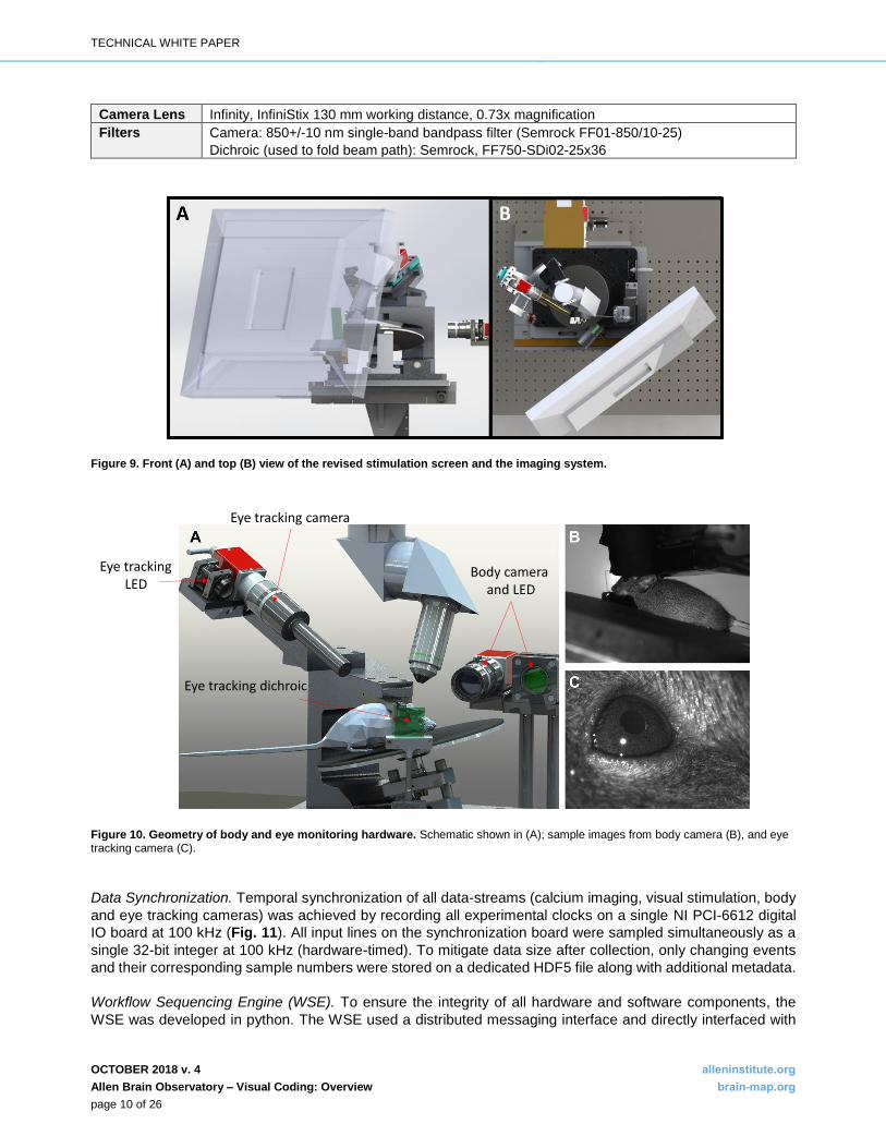
Mouse body and eye monitoring. During calcium imaging experiments, eye movements and animal posture

were recorded (Fig. 10A). The left side of each mouse was imaged with the stimulation screen in the

background (Fig. 10B) to provide a detailed record of the animal response to all stimuli. The eye facing the

stimulus monitor (right eye) was recorded (Fig. 10C) using a custom IR imaging system. No pupillary reflex was

evoked by any of these illumination LEDs.

Table 1. Hardware for behavior and eye monitoring.

Behavior Monitoring Hardware

Camera Allied Vision, Mako G-032B - GigE interface

30 fps. 33 ms exposure time, camera hardware gain: 10

Illumination LED Engine Inc., LZ4-40R308-0000 - 740 nm

Camera Lens Thorlabs MVL8M23, 8 mm EFL, f/1.4, for 2/3" C-Mount Format Cameras, with lock

Filters Camera: a 785 nm short-pass filter (Semrock, BSP01-785R-25) suppressed light from the eye-

tracking LED.

Illumination: a 747+/-33 nm bandpass filter (Thorlabs, LB1092-B-ML) in front of the LED

prevented visible portion of the LED spectrum from reaching the mouse eye.

Eye Monitoring Hardware

Camera Allied Vision, Mako G-032B with a GigE interface, used at 30 fps, 33 ms exposure time, camera

hardware gain of 10-20

Illumination LED Engin Inc., LZ1-10R602-0000 (850 nm)

Lens in front of the LED : Thorlabs, LB1092-B-ML

Stimulation screen

Stimulation screen

15 cm




page 10 of 26

Camera Lens Infinity, InfiniStix 130 mm working distance, 0.73x magnification

Filters Camera: 850+/-10 nm single-band bandpass filter (Semrock FF01-850/10-25)

Dichroic (used to fold beam path): Semrock, FF750-SDi02-25x36

Figure 9. Front (A) and top (B) view of the revised stimulation screen and the imaging system.

Figure 10. Geometry of body and eye monitoring hardware. Schematic shown in (A); sample images from body camera (B), and eye tracking camera (C).

Data Synchronization. Temporal synchronization of all data-streams (calcium imaging, visual stimulation, body

and eye tracking cameras) was achieved by recording all experimental clocks on a single NI PCI-6612 digital

IO board at 100 kHz (Fig. 11). All input lines on the synchronization board were sampled simultaneously as a

single 32-bit integer at 100 kHz (hardware-timed). To mitigate data size after collection, only changing events

and their corresponding sample numbers were stored on a dedicated HDF5 file along with additional metadata.

Workflow Sequencing Engine (WSE). To ensure the integrity of all hardware and software components, the

WSE was developed in python. The WSE used a distributed messaging interface and directly interfaced with

Eye tracking camera

Eye trackingLED

Body camera and LED

Eye tracking dichroic




page 11 of 26

the microscope software (Scientifica SciScan and Nikon Elements), the stimulation computer, the

synchronization computer as well as the body and eye-tracking computer. Where instrumentation changes

required user intervention, the WSE prompted the rig operator to initiate and acknowledge completion of manual

tasks. Finally, the WSE packaged all data streams and automatically triggered data transfer to a centralized

data repository.

Figure 11. Schematic diagram of the data synchronization architecture for two-photon imaging experiments.

Calcium Imaging Data Collection. All two-photon imaging experiments were conducted under ambient red light

to maintain the reversed day-night cycle. Mice were head-fixed on top of a rotating disk and free to walk at will.

The disk was covered with a layer of removable foam (Super-Resilient Foam, 86375K242, McMaster) to

alleviate motion-induced artifacts during imaging sessions.

A dataset consisted of three experiments (~90 min each) at a given location (cortical area and depth) during

which mice passively observed three different stimulus protocols (see whitepaper on “Stimulus Set and

Response Analysis” in Documentation). The same location was targeted for imaging on all three recording days

to allow repeat comparison of the same neurons across sessions. A dataset was collected per day, for a total

of 16 sessions over the course of a full multi-day experimental series.

On the first day of imaging at a new location, the targeting map (Fig. 5F) was used to select spatial coordinates.

The XYZ stage under the mouse was used to move the animal holder to position the imaging objective above

the target location. Comparison of superficial vessel patterns were used to verify the appropriate location by

imaging over a field of view of ~800 µm using epi-fluorescence and blue light illumination. Once a cortical region

was selected, the objective was shielded from stray light coming from the stimulation screen using black tape.

In two-photon imaging mode, the desired depth of imaging was set to record from a specific cortical layer. On

subsequent imaging days, a return to the same location was achieved using three alignment steps (Fig. 12):

1. The pattern of vessels was matched to those from the previous imaging day in epifluorescence mode

using a red-green overlay of live acquisition with a reference image from the previous day.

2. Using the overlay, the same vessels were matched in two-photon mode using a surface image acquired

in the previous session so as to provide adequate coverage of the two-photon field of view (~400 µm).





page 12 of 26

3. Once at depth, the current image was matched with a previous depth image using fine stage

movements (+/- 5 µm) and grid overlay (100 µm pitch) displayed on the reference and target live

images.

Figure 12. Illustration of the alignment procedure to record from the same population on different days, using surface vasculature for field of view alignment.

Once a depth location was stabilized, a combination of PMT gain and laser power was selected to maximize

laser power (Table 2) and dynamic range while avoiding pixel saturation (max number of saturated pixels

<1000). The stimulation screen was clamped in position, and the experiment began.

Two-photon movies (512x512 pixels, 30Hz), eye tracking (30Hz), and behavior (30Hz) were recorded and

continuously monitored. Recording sessions were 1 hour long but were interrupted if any of the following was

observed: 1) mouse stress as shown by excessive secretion around the eye, nose bulge, and/or abnormal

posture; 2) excessive pixel saturation (>1000 pixels) as reported in a continuously updated histogram; 3) loss

of baseline intensity caused by bleaching and/or loss of immersion water in excess of 20%; 4) hardware failures

causing a loss of data integrity.

Table 2. Maximum laser power used per depth range.

Immersion water was supplemented at times while imaging

using a micropipette taped to the objective (Microfil MF28G67-

5 WPI) and connected to a 5 ml syringe via an extension tubing.

This ensured that baseline intensity stayed within 5% of the

original intensity level and allowed water level adjustments to

be made without interrupting an experiment. At the end of each

experimental session, a z-stack of images (+/- 30 µm around

imaging site, 0.1 µm step) was collected to evaluate cortical

anatomy. In addition, for each experimental area analyzed, a

full-depth cortical z stack (~700 µm total depth, 5 µm step) was

collected to document the imaging site location.

Data Processing for Two-Photon Calcium Images

Deconvolution. The images acquired from the custom Nikon (but not Scientifica) two-photon microscopes used

in these studies exhibited fluorescence leakage between nearby pixels. As the galvonometer moved horizontally




page 13 of 26

across the field of view, fluorescence from one pixel was “carried over” to successive pixels (Fig. 13 A). This

pixel leakage artificially correlated adjacent pixels and potentially contaminated signal between cells. To

characterize the artifact, the recorded fluorescence was modeled as a “corrupted” version of the true image. By

estimating the form of that corruption, an approximation of the true, un-corrupted image was calculated. The

pixel leakage was not uniform across the image, with pixels near the center of the field of view exhibiting wider

leakage than those near the edges. The shape of this non-uniformity was well fit by a sinusoid, suggesting that

it could be due to the speed of the galvanometer (Fig. 13B, C).

Figure 13. Pixel leakage in Nikon microscopes. A) Example dark frame excerpt from one of the Nikon microscopes. The photon shot noise, rather than being contained to one pixel, is horizontally blurred in the direction of the galvanometer movement. B, Width of shot noise transients vs horizontal location from 899 dark frames (black dots) taken on microscope 1 (B) and microscope 2 (C), and sinusoidal fit (red line).

In order to correct for this leakage, a filter was constructed to return an estimate of the true image. For each of

the two Nikon microscopes, 899 dark-field images were acquired. For each image, the width of the shot noise

was computed as a function of horizontal location in the image. To describe the warping of the pixel leakage in

each microscope, a sinusoid is fitted to the relationship of shot noise width vs horizontal location in the image.

This sinusoid was used to warp each image, stretching it so that the pixel leakage was uniform across horizontal

locations (Fig. 14).

Each image was flattened such that a warped image formed a pixel series (𝒚𝑀) concatenating rows in the order

and direction in which the galvometer scanned. An artificial time series was also applied (𝒚𝑇) with delta pulses

at the beginning of each instance of the shot noise. The leakage filter 𝑯 was estimated as �̃� = �̃�𝑀 �̃�𝑇⁄ , where

�̃� is the Fourier transform of 𝑯. This yielded an estimate of the filter describing pixel leakage in each microscope.

The estimated leakage filters were used to apply a regularized Wiener deconvolution to the linear pixel series

of each image. A recorded pixel series (𝒚) was modeled (first warping the 2D image to make the leakage

spatially uniform, and then unraveling it into the pixel series) as �̃� = �̃�𝒙 + �̃�, where 𝐻 is the leakage filter and

𝜂 is measurement noise. Under a smoothness constraint on the image, the leakage-corrected pixel series was

obtained as 𝒙 = �̃��̃� with �̃� =𝟏

�̃�(

|�̃�|𝟐

|�̃�|𝟐

+𝝀𝜦�̃�). 𝚲 is the Laplacian operator, implementing the smoothness constraint.

The parameter 𝜆 = 0.1 weights the smoothness constraint. This was chosen by examining the autocorrelation

of the deconvolved pixel series from 100 randomly selected frames from two movies, taking into account the

width at half max of the autocorrelation function and the number of local maxima in the autocorrelation function

surrounding 0-pixel lag. For 𝜆 ≈ 𝟎, the noise amplification inherent in deconvolution caused ringing in the pixel

autocorrelation while for 𝜆 ≳ 0.3, the pixel autocorrelation was artificially widened.

After deconvolution of the leakage from the pixel series 𝒚, negative fluorescence values were corrected to the

maximum of 0 and the mean fluorescence within a 5-pixel radius, then un-warped the image back to its original

dimension and aspect ratio (Fig. 14). The effect of the deconvolution is apparent in maximum intensity

projections of the same movie before and after deconvolution (Fig. 15); after deconvolution, the images are

spatially sharpened.




page 14 of 26

Figure 14. Illustration of deconvolution. Each panel shows the same imaging frame at each step of the deconvolution process. Following the arrows: Original image frame, Image after warping to make pixel leakage spatially uniform so that it can be deconvolved, Deconvolved image, still in warped coordinates, Deconvolved and un-warped image frame.

Figure 15. Maximum-intensity projections of a two-photon movie, before and after deconvolution of the Nikon pixel leakage. A) Full frames. B) Zoom-in of the red rectangles of panel A. Left column: original images, right column: after deconvolution. The deconvolved images are spatially sharpened, reflecting the correction for the blur induced by the fluorescence leakage.

Motion Correction. The two-photon calcium imaging videos exhibited non-trivial frame-to-frame motion artifacts

likely due to animal or brain motion. Computing globally optimal frame-to-frame alignment across for ~1M frame

videos is computationally expensive, so a 2-stage hierarchical motion correction algorithm was developed.

The first stage subdivided the video into contiguous 400 frame sections. All frames within a section were

registered to the section's average image via rigid-body phase correlation after padding with a Hanning window.




page 15 of 26

After alignment, the average image was recomputed and individual frames were realigned to the new average.

This iterative refinement process is repeated three times per section.

Section-to-section alignment was performed iteratively in the same manner. The average images produced

from within-section alignment were aligned to their average via phase correlation six times. Finally, individual

frames were aligned to their globally aligned section average frames.

Overview of Cell Segmentation and Region of Interest (ROI) Filtering. The active cell segmentation module was

designed to locate active cells within a field-of-view (FOV) by isolating cellular objects using the spatial and

temporal information from the entire movie. The goal of the active cell segmentation module is to achieve robust

performance across experimental conditions with no or little adjustment, such as different mouse cell lines,

fluorescent proteins (e.g., GCaMP6f or GCaMP6s), and FOV locations of visual areas and depths. The process

begins with the full image sequence as input to apply both the spatial as well as temporal information to isolate

an individual active cell of interest without data reduction, such as by PCA, and does not make assumptions

about the number of independent components existing in the active cell movie. Also, in contrast to other

methods, this approach separates the individual steps, including identifying and isolating each cellular object,

computing confidence of each identified object (by object classification) and the step of resolving objects

overlapping in x-y space (which lead to cross talk in traces), so that each can be improved upon if necessary.

Presegmentation. The motion corrected image sequence was spatially median filtered (using 3x3 pixel kernel)

to reduce white noise. The sequence was then low pass filtered and downsampled by 1/8 temporally to enhance

the signal-to-noise ratio (SNR). The processed image sequence was then divided into periods of fixed temporal

length p, where p = 50 frames (~13.3 sec.). The maximum projection image from each period and the mean

image (mu_image) of the whole sequence were computed. The maximum projection image from all temporal

periods, called Periodical Projection frames PP(t), were further normalized to become Normalized Periodical

Projection (NPP) frames:

NPP(t) = MF((PP(t) – mu_image), 3x3) * G(t)

Where G(t) is the frame intensity normalization gain computed based on the intensity histogram of each PP(t).

This is to normalize any change in overall intensity across the experiment, and to reduce experiment-to-

experiment variability. MF(3x3) is median filtering with a 3x3 pixel kernel (Fig. 16 C).

Note in each NPP(t), a subset of cells can be found with changes in fluorescence during that time period. With

sufficient experiment length, and with many sweeps of different stimuli, various repetitive cell firing patterns can

be found. Cells with overlapping spatial positions in x and y can be observed as firing at different time frames,

allowing the following detection process to identify them individually despite having spatial overlap.

Detection. Adaptive and mathematic morphological image processing techniques were applied to process each

NPP(t). After band-pass filtering, an initial binary object map was generated by thresholding the resulting image

minus a low pass version of itself to capture spatially varying background intensity. Conditional dilation, erosion

and connected component analysis were applied to filter the candidate binary objects and fill holes. The final

set of regions of interest (ROIs) in each NPP were identified using another connected component labelling and

a simple rule-based classifier. This classification was based on comparing measured morphometric attributes

(object area, shape, intensity, uniformity, etc.) of the objects to the statistics derived from the targeted active

cell components in the sample data sets. After each frame was processed, a set of candidate ROIs from each

NPP were then grouped with candidate ROIs from all other NPPs. ROIs within a similar spatial location (defined

by the distance between centroids < 5 µm) and with similar morphometric attributes (e.g., delta (area or shape)

< 20%) across NPP frames were grouped as the same cell object. The ROI with the highest contrast and with

shape and area within range statistically derived from sample data was selected to represent that cell in the

mask image and in a composite image for visual QC. ROIs with different spatial locations (centroids > 5 µm

apart) and or dissimilar morphometric attributes are recorded as different cells (Fig. 17B, C).




page 16 of 26

Figure 16. Presegmentation. A, Maximum projection image of an experiment. Note some cell bodies are not clearly visible in the busy background and neuropil, often due to overlap with other objects. B, Boundaries of detected active cells by the segmentation algorithm is shown. Many overlapping cellular objects not easily visible in the projection image were successfully identified and isolated because detection operates in both temporal and spatial space. C, Examples of consecutive NPP(t) images. Contrast of firing cells are enhanced by reducing background (see definition of NPP(t)).

Occasionally two or more spatially overlapping ROIs could be found that were active in the same timeframe

and were therefore detected as a single ROI for that NPP. Additional steps to classify them as multiple-cell

objects were taken using their attributes of combined area and shape (eccentricity).

After ROI detection in each NPP frame and grouping of all ROIs across frames was completed, a set of “unique”

active cell objects was identified (Fig. 17B). Cells near the FOV boundaries (3 µm) were eliminated from further

consideration due to the fact that motion shifts can create boundary effects to the traces computed from these

cells. To generate the segmentation mask image, all non-overlapping cells were placed in a single mask plane

and overlapping cells were placed in subsequent planes, to ensure unique identification of all cells (Fig. 17C).

ROI Filtering. Not all ROIs generated by segmentation are complete individual cell bodies. To exclude ROIs

that are not actually cell bodies from further analysis, the ROIs are labeled with a multi-label classifier where

any ROIs that end up labeled are not considered cell bodies. The set of reasons to exclude an ROI are: the ROI

is a union of two or more cells; the ROI is a duplicate of another; the ROI is close to the edge of the FOV and

is impacted by motion such that parts of the ROI are missing from the video; the ROI is likely an apical dendrite

and not a cell body; or that the ROI is too small, too narrow, or too dim to confidently be considered a cell body.

The initial ROI filtering was generated by a set of heuristics based on depth, shape, area, intensity, signal-to-

noise, and the ratio of mean to max intensity of the max projection. The initial filtering was used to generate a

set of training labels, on which a multi-label classifier was trained. The multi-label classifier is implemented using

a linear Support Vector Classifier trainer for each label (binary relevance) using metrics generated in

segmentation combined with depth, driver, reporter, and targeted structure as features. The final ROI filtering

workflow is to 1) label ROIs that fall within the motion cutoff regions at the border, 2) label ROIs using the binary

relevance classifier, 3) label significantly overlapping ROIs as duplicates, and 4) label ROIs that significantly

overlap two or more ROIs as unions.




page 17 of 26

Figure 17. ROI detection. A, Maximum projection image of another experiment. B, Boundaries of detected active cells by the segmentation algorithm is shown. One area with overlapping cells is highlighted in red. C, Mask of detected overlapping cells are placed in different planes for trace calculation.

Demixing traces from overlapping ROIs. The simplest way to extract fluorescence traces, given a set of ROI

masks, is to average the fluorescence within each ROI. If two ROIs overlap, this procedure will artificially

correlate their traces. Therefore, a model is used where every ROI has a trace which is distributed across its

ROI in some spatially heterogeneous, time-dependent fashion:

𝐹𝑖𝑡 = ∑ 𝑊𝑘𝑖𝑡𝑇𝑘𝑡

𝑘

where W is a tensor containing time-dependent weighted masks: 𝑊𝑘𝑖𝑡 measures how much of neuron 𝑘’s

fluorescence is contained in pixel 𝑖 at time 𝑡. 𝑇𝑘𝑡 is the fluorescence trace of neuron 𝑘 at time 𝑡 - this is the

desired value to estimate. 𝐹𝑖𝑡 is the recorded fluorescence in pixel 𝑖 at time 𝑡.

Importantly, this model applies to all ROIs, including those too small to be a neuron or otherwise filtered out.

Duplicate ROIs (defined as two ROIs with >70% overlap) and ROIs that are the union of two other ROIs (any

ROI where the union of any other two ROIs accounts for 70% of its area) are filtered out before demixing, and

the remaining filtering criteria are applied after demixing. Projecting the movie (𝐹) onto the binary masks (𝐴)

reduces the dimensionality of the problem from 512x512 pixels to the number of ROIs:

∑ 𝐴𝑘𝑖

𝑖

𝐹𝑖𝑡 = ∑ 𝐴𝑘𝑖𝑊𝑘𝑖𝑡𝑇𝑘𝑡

𝑘,𝑖

where 𝐴𝑘𝑖 is one if pixel 𝑖 is in ROI 𝑘 and zero otherwise–these are the ROI masks from segmentation, after

filtering out duplicate and union ROIs. At a particular time point 𝑡, this yields the simple linear regression:

𝐴𝐹(𝑡) = (𝐴𝑊𝑇(𝑡))𝑇(𝑡)




page 18 of 26

where the weighted masks 𝑊 are estimated by the projection of the recorded fluorescence 𝐹 onto the binary

ROI masks 𝐴. On every imaging frame 𝑡, the linear least squares solution �̂� are computed in to extract each

ROI’s trace at that time point.

It was possible for ROIs to have negative or zero demixed traces �̂�. This occurred if there were union ROIs

(one ROI composed of two neurons) or duplicate ROIs (two ROIs in the same location with approximately the

same shape) that the initial detection missed. If this occurred, those ROIs and any that overlapped with them

were removed from the experiment. This led to the loss of ~1% of ROIs.

Neuropil Subtraction. The recorded fluorescence from an ROI was contaminated by the fluorescence of the

neuropil immediately above and below the cell due to the point-spread function of the microscope. In order to

correct for this contamination, the amount of contamination was estimated for each ROI. The estimated 𝐹𝑁 was

done by taking an annulus of 10 m around the cellular ROI, excluding pixels from any other ROIs. In order to

remove this contamination, the extent to which ROI was affected by its local neuropil signal was evaluated.

The recorded traces were modeled as 𝐹𝑀 as 𝐹𝑀 = 𝐹𝐶 + 𝑟𝐹𝑁, where 𝐹𝐶 is the unknown true ROI fluorescence

trace and 𝐹𝑁 is the fluorescence of the surrounding neuropil. In order to estimate the contamination ratio 𝑟 for

each ROI, the error was minimized 𝐸 = ⟨(𝐹𝐶 − (𝐹𝑀 − 𝑟𝐹𝑁))2

+ 𝜆Λ(𝐹𝐶)⟩𝑡 by jointly optimizing for 𝑟 and 𝐹𝐶. Λ(𝐹𝐶)

is the first temporal derivate of the cellular trace, weighted by 𝜆 = 0.05; this smoothness constraint on the cellular

trace allows per-ROI optimization for 𝑟. ⟨∙⟩𝑡 denotes an average over time. Gradient descent was used on 𝑟. At

each step of the gradient descent, 𝐹𝐶 was solved at the zero gradient of 𝐸. Gradient descent was performed

on the first half of the traces and computed 𝐸 on the second, so that it is a cross-validation error. After computing

𝑟 and 𝐹𝐶 for an ROI, the neuropil-subtracted trace 𝐹𝑀 − 𝑟𝐹𝑁 was used as the basis for all subsequent analysis

in order to avoid any residual effects of the smoothness constraint.

Figure 18. Example of original ROI and neuropil traces, and neuropil-subtracted ROI trace.

ROI 149 from experiment 502199136, with r=.79.




page 19 of 26

Figure 19. Distribution of contamination ratios (left) and cross-validation errors (right) for an example experiment (502199136). For this experiment, neuropil subtraction failed on 8% of cells (16/199).

To standardize the learning rate and initial conditions of the gradient descent, each ROI’s neuropil trace was

normalized to (0,1). The measured ROI trace was normalized by the same amount, used a learning rate of 10

and initial condition of 𝑟 = 0.001. The gradient descent was stopped at the first local minimum of 𝐸. If the

resulting 𝑟 was greater than 1 or less than 0, or final cross-validation error 𝐸 greater than 2 |⟨𝐹𝑀⟩𝑡|, the gradient

descent was attempted again with a 10x slower learning rate. If those convergence criteria were still not met,

an initial condition of 𝑟 = 0.5 was used. If those convergence criteria were still not met, that ROI was flagged

and after computing 𝑟 for all other ROIs in the experiment, set 𝑟 for un-converged ROIs to the mean.

To validate the performance of our algorithm, it was tested on a publicly-available benchmark dataset (Chen et

al., 2013). A distribution of contamination ratios was obtained, centered nearly on the author’s choice of 0.7

(mean r of 0.68 vs their choice of 0.7), but with significant heterogeneity (Figs 20, 21). For this benchmark

dataset and using the same optimization parameters as for the Allen Brain Observatory – Visual Coding

data, 6 of 36 cells failed the initial neuropil subtraction with r>1, and would have gone through the additional

steps outlined above.

Figure 20. Example results of neuropil subtraction from the benchmark dataset. Fluorescence vs time (sec).




page 20 of 26

Figure 21. Summary of neuropil subtraction on a benchmark dataset. Left, histogram of contamination ratios on the 36 cells of the GCaMP6f data of Chen et al., 2013. Mean: 0.68, Standard deviation: 0.38. Right, histogram of the corresponding cross-validation errors.

Optical physiology (ophys) session matching: Multiple two-photon calcium imaging movies were acquired for

each field of view across 3 imaging sessions (one experiment) using different visual stimuli. To map cells

between sessions, an automated matching module was developed. The module used average intensity

projection images and the segmented cell mask images of experiments with stimulus A, B, and C as inputs,

and produced a lookup table that grouped the same cells identified across different sessions. Three cell mask

images with unified labeling of cells across all three sessions were also generated.

Figure 22. Mapping between cells across 3 optical physiology data acquisition sessions. Top row: Maximum intensity projection image from each experiment. Middle row: All identified objects for each session. Colors represent uniquely identified cells. Grey outlined objects did not meet classification criteria based on measured morphometric attributes (object area, shape, intensity, uniformity, etc.) Numbers of identified objects per session: A: 215 cells, B: 213 cells, C: 191 cells. Bottom row: Cells identified across all 3 sessions. Matching cells are labeled with the same color in each of the mask images. 127 cells were present in all sessions A, B and C.




page 21 of 26

The module first used an intensity-based method to register the average intensity projection images of experiments B and C to that of the reference experiment A, producing an affine transformation that brings together all the experiments to a standard canonical space. This computed transformation was used to map the segmented cell mask images to a canonical space, so that cells in these images were spatially related. To map cells, a bipartite graph matching algorithm was used to find correspondence of cells between experiment A and B, A and C, as well as B and C. The algorithm used cells in the pair-wise experiments as nodes, and the degree of spatial overlap and closeness (both normalized) between cells in the two experiments as weight of edge of the nodes. By maximizing the summed weights of edges, the bipartite matching algorithm found the “best match” between cells in each pair of experiments (Fig. 22). Finally, a label combination process was applied to the matching results of A and B, A and C, as well as B and C, producing a unified label for all three experiments.

Response Metrics. Response metrics are defined in the “Stimulus Set and Response Analysis” whitepaper in Documentation.

Eye tracking analysis algorithm

Videos of the ipsilateral eye (relative to the monitor) were used to extract pupil location and size. Coordinates

for eye position were extracted independently for each frame of the eye position movie.

Pupil identification. In order to identify the region of the image corresponding to the pupil, a variant of the star-

burst algorithm was used (Li, Winfield and Parkhurst, 2005; Zoccolan, Graham and Cox, 2010). This algorithm

fits an ellipse to the pupil or corneal reflection (CR) area, respectively. The areas for both the pupil and CR were

identified with essentially the same method. This proceeds in several stages.

Figure 23. Sequence of steps for eye tracking analysis.

First, the initial seed points for the pupil and corneal reflection were set (Fig. 23-A). These points were identified via a convolution with a black square (for the pupil) or a bright square against a black background (for the CR). To fit the ellipse, 18 rays were drawn starting at the seed point, spaced 20 degrees apart (Fig. 23-B). For each ray, the initial 10 pixels along that ray were averaged (call this value a_0). A candidate boundary point was





page 22 of 26

calculated for the pupil by choosing the pixel along the ray that first exceeds the threshold F*a_0, where F is an input parameter to the algorithm (often around 1.5, but varies by experiment; Fig. 23-C). For the CR, the first point below this threshold is used. During development, the gradient was too noisy to consistently identify the boundary points. A RANSAC algorithm is used to fit the ellipse from the candidate boundary points using linear regression with a conic section constraint. The fit parameters from the regression are converted into the five ellipse parameters: x,y location of the center, the major and minor axis sizes, and the angle of rotation with respect to the x-axis (Fig. 23-D). The pupil and CR ellipse fit parameters are converted into coordinates for the location of the pupil in a coordinate system centered in the mouse eye, which is assumed spherical (an approximation) and thus acts as a spherical mirror. The location of the CR in the mouse eye coordinate system is thus a vector of length r_0/2 in the direction of the LED (where r_0 is the radius of the mouse eye). This is used along with the camera and monitor positions to reconstruct the pupil position elevation and azimuth relative to the center of the monitor. The pupil area is reported as the area of the ellipse fit to the pupil region: pi*major_axis^2. In some cases, the algorithm did not find appropriate parameters for the ellipses describing the pupil or corneal reflection. In other cases, outlying values were detected (based on overall area or discontinuous jumps in the location, for example) that are clearly not physical values of the pupil or corneal reflection. In these cases, the pupil position is reported as NaN.

Screening procedure for abnormal activity resembling inter-ictal events

A comprehensive analysis of previously collected experiments revealed abnormal calcium activity in some

experiments in mice with widespread expression of GCaMP6. Local Field Potential recordings were compared

across C57BL/6J mice and various GCaMP6-expressing transgenic mice (Steinmetz et al., 2017) which

confirmed the presence of unusually large (>1 mV), long (width >10 ms) and correlated events in large portions

of the dorsal cortex in affected animals. These events resemble epileptiform inter-ictal events.

These widespread correlated events could be detected using wide-field calcium imaging (FOV width >5 mm).

These events were more easily detected in the somatosensory cortex than in visual cortex, and become more

widespread as the mice aged. Their occurrence was quantified using an event detection algorithm: the averaged

ΔF/F fluorescence trace of the entire FOV was extracted, and the FWHM width in ms of all local maxima peaks,

as well the prominence of all of these peaks was computed, as described:

https://en.wikipedia.org/wiki/Topographic_prominence.

To screen for affected animals prior to imaging, a 5 min long epifluorescence movie over the somatosensory

cortex was collected during the habituation session (FOV width = 800 μm). Each movie was analyzed using the

prominence/width plot (Fig. 24) and mice showing abnormal clusters of events (width <300 ms and amplitude

>10%) were excluded from subsequent analysis. Furthermore, after data collection, every two-photon movie

session was screened for the presence of these events using the same prominence/width plot; affected data

was discarded, and mice were excluded from further data collection. Previously released affected datasets are

indicated in the http://observatory.brain-map.org/visualcoding data portal and in Transgenic Characterization

documentation.

https://en.wikipedia.org/wiki/Topographic_prominence

http://observatory.brain-map.org/visualcoding




page 23 of 26

Figure 24. Quantification of full FOV calcium events amplitude and width. Prominence and width of all detected calcium events in a 5 min recording sessions using two photon calcium imaging. Left: example plot in a transgenic mouse expressing GCaMP6f under the Cux2 promoter. Right: example plot in a transgenic mouse expressing GCaMP6f under the Emx1 promoter. Note the abnormal presence of large and fast events.

Data file content and format: NWB file

All processed optophysiology data is published in the Neurodata Without Borders (NWB) file format

(www.nwb.org). The NWB is an HDF5 file that contains:

Experimental metadata, including:

o Make and model of 2-photon microscope, display monitor, and eye tracking camera

o Microscope field of view, in microns and pixels and movie resolution (pixel_size)

o Animal metadata including specimen genotype, specimen identifier, age in days, sex o Imaging location: Depth from brain surface (z), Targeted brain area (x, y)

Segmented ROI masks

ROI Mean fluorescence traces Motion correction information ROI DF/ F traces ROI Neuropil mean fluorescence traces

ROI R and RMSE values computed via the neuropil subtraction algorithm Timestamped stimulus presentation description tables

Stimulus templates (images, movies) Eye tracking data Running speed

Neuropil-subtracted traces can be derived from each ROI's raw fluorescence trace, neuropil trace, and

computed R value. Code that performs this computation is available in the Allen Software Development Kit

(AllenSDK).

Availability of raw 2-photon calcium fluorescence movies

Motion-corrected 2-photon calcium fluorescence movies are too large to download directly, and are available

upon request. Each experiment contains three movie files of approximately 60 GB each. To receive raw movies,

the requestor must send one or more hard drives with sufficient capacity to store the files and a shipping account

number to cover the cost for the return of the hard drive(s). In some cases, alternate data transfer can be

arranged through cloud share services. Data is provided under the Allen Institute Terms of Use.

www.nwb.org

http://www.alleninstitute.org/legal/terms-use/




page 24 of 26

To request raw movie data files, contact us and provide:

Experiment IDs for desired movies

Point-of-contact name, organization, shipping and email addresses

Upon receipt of this request, the requestor will be contacted to arrange file transfer, usually within two weeks of

the receipt of a storage drive.

Quality Review for Two-Photon calcium imaging

Each experiment was reviewed for integrity based on a broad range of operational parameters. A

comprehensive report was automatically generated to track data trends, animal behavior, experimental failures

and errors. In particular:

Photonic saturation did not exceed 1000 pixels and the full dynamic range of the recording system was

adequately covered.

Baseline fluorescence did not drop below 20% baseline levels at any particular point during the experiment.

Cell matching across sessions was manually verified for every experiment using 500 frames averages

across different days.

Stability of image recording was assessed by using a z-stack of images (+/- 30 μm around imaging site, 0.1

μm step), collected at the end of each experimental session. Experiments with z-drift above 10µm over the

course of the entire session were excluded.

Animals did not show excessive signs of stress. Any animal that showed eye secretion covering the pupil

or excessive orbital tightening was returned to its home cage to recover. The presence of nose bulge, flailing

and abnormal postures was also monitored.

Surgery monitoring. Analyzing the reproducibility of visual areas from the initial ISI imaging session (T0 weeks,

n=147) to the subsequent ISI imaging session (T4 weeks, n=81) presented consistent results from the two time

points. For same animals over time, six visual areas are consistently identified: VISp, VISl, VISal, VISrl, VISam,

and VISpm. Visual area size, as well as coverage of the retinotopic ranges remained the same over an interval

of 4 weeks. A decision was made to replace the second intrinsic imaging session used in a previous data

release (2016) with a simple capture of the vessel image to follow the stability of the cortical window.

Following two-photon calcium imaging, an image of the animal’s brain surface vasculature is captured with

green LED illumination. The image serves as brain health monitoring stop at this stage of the workflow.

SERIAL TWO-PHOTON TOMOGRAPHY

Volumetric image acquisition by serial two-photon tomography

Serial two-photon tomography was used to obtain a 3D image volume of coronal brain images for each

specimen. This image series enables spatial registration of each specimen’s associated ISI and optical

physiology data to the Allen Mouse Common Coordinate Framework (CCF). By coupling high-speed multi-

photon microscopy with automated vibratome sectioning on a dimensionally stable tissue block, this imaging

platform greatly reduces deformations commonly occurring with conventional section-based histological

methods and provides a series of high-resolution images in pre-aligned 3D space. Methods for this procedure

have been described in detail in whitepapers associated with the Allen Mouse Brain Connectivity Atlas in

Documentation for that resource, and in the associated publication by Oh, et al (2014).

Mice were anesthetized with 5% isoflurane and intracardially perfused with 10 ml of saline (0.9% NaCl) followed

by 50 ml of freshly prepared 4% paraformaldehyde (PFA) at a flow rate of 9 ml/min. Brains were rapidly

dissected and post-fixed in 4% PFA at room temperature for 3-6 hours and overnight at 4°C. Brains were then

rinsed briefly with PBS and stored in PBS with 0.02% sodium azide before proceeding to the next step. Agarose

was used to embed the brain in a semisolid matrix for serial imaging. After removing residual moisture on the

surface with a Kimwipe, the brain was placed in a 4% oxidized agarose solution made by stirring 10 mM NaIO4

http://allins.convio.net/site/PageServer?pagename=send_us_a_message

http://help.brain-map.org/display/mouseconnectivity/Documentation




page 25 of 26

in agarose, then transferring through 50 mM phosphate buffer and embedding at 60°C in a grid-lined embedding

mold to standardize placement of the brain in an aligned coordinate space (Fig. 25). The agarose block was

then left at room temperature for 20 minutes to allow agarose to solidify, and then covalent interaction between

the brain tissue and the agarose was promoted by placing the block in 0.2% sodium borohydride in 50 mM

sodium borate buffer (pH 9.0) for 48 hours at 4°C. The agarose block was then mounted on a 1x3 glass slide

using Loctite 404 glue in preparation for serial imaging.

Figure 25. Embedding specimen in agarose. Each specimen was aligned in the middle of an agarose block so that the anterior-posterior axis was perpendicular to the bottom and parallel to the vertical axis of the mold. Top (left panel) and side (right panel) views are shown.

Serial two-photon (STP) tomography is described by TissueVision, Inc. (Ragan, 2012), and in the technical

whitepapers of the Allen Mouse Brain Connectivity Atlas and by Oh, et al (2014). Multi-photon image acquisition

was performed using a customized TissueCyte 1000 system (TissueVision, Cambridge, MA) coupled with an

ultra-fast mode-locked Ti:Sapphire laser.

First the mounted specimen was placed on the metal plate in the center of the cutting bath, which was filled with PBS with 0.02% sodium azide and placed onto the sample stage. For best results, a new vibratome blade was used for each specimen and aligned to be parallel to the leading edge of the specimen block. Next, the top surface of the specimen block was brought up to the level of the vibratome blade by adjusting the sample stage height. The z-stage was set to slice at 100 μm intervals. Specimens were oriented for image acquisition to occur from the caudal to the rostral end. Boundaries for each edge of the specimen were defined, such that the XY scan area of the entire brain was estimated. The XY scan area consists of 221 tiles (17 rows x 13 columns). Each tile was imaged at a resolution of 832x832 pixels. The specimen was illuminated with a 925 nm wavelength laser. The excitation beam was directed to 75 μm below the cutting plane of each specimen by moving the objective using a piezo-controller (Physik Instrumente, Karlsruhe, Germany). This depth was selected as it is deep enough to minimize deformations at the cutting surface caused by vibratome sectioning but shallow enough to retain sufficient photon penetration for high contrast images. Thus, the optical plane of section is at 75 μm below the slicing surface, with an illumination field area of approximately 3-4 μm ellipsoidal depth.

A Zeiss 20x water immersion objective (NA = 1) was used to focus the light on the sample and to direct

fluorescence through the emission path of the system. A 560 nm dichroic (Chroma, Bellows Falls, VT) split the

emission light, and a 500 nm dichroic (Chroma) further split the emission for a total of three channels. The

593/40 nm (Chroma), 520/35 nm (Semrock, Rochester, NY) and 447/60 nm emission filter (Chroma) were used

for the Red, Green and Blue channels, respectively. The three photomultiplier tubes (R3896, Hamamatsu,

Bridgewater, NJ) were used to detect the emission at each channel. In order to scan a full tissue section,

individual tile images were acquired, and the entire stage (Physik Instrumente) was moved between each tile.

After an entire section was imaged, the X and Y stages moved the specimen to the vibratome, which cut a 100

µm section and returned the specimen to the objective for imaging of the next section. The blade vibrated at 60

Hz and the stage moved toward blade at 0.5 mm/sec during cutting.

http://help.brain-map.org/display/mouseconnectivity/Documentation




page 26 of 26

REFERENCES

Chen TW, Wardill TJ, Sun Y, Pulver SR, Renninger SL, Baohan A, Schreiter ER, Kerr RA, Orger MB, Jayamaran

V, Looger LL, Svoboda K, Kim DS. (2013) Ultrasensitive fluorescent proteins for imaging neuronal activity.

Nature, 499(7458):295-300.

Garrett ME, Nauhaus I, Marshel JH, Callaway EM. (2014) Topography and areal organization of mouse visual

cortex. J Neurosci., 34(37):12587-600.

Goldey GJ, Roumis DK, Glickfield LL, Kerlin AM, Reid RC, Bonin V, Andermann ML. (2014). Versatile cranial

window strategies for long-term two-photon imaging in awake mice. Nature Protocols, 9(11):2515-2538.

http://doi.org/10.1038/nprot.2014.165

Kalatsky VA and Stryker MP. (2003) New Paradigm for Optical Imaging: Temporally Encoded Maps of Intrinsic

Signal. Neuron, 38:529–545.

Li, D., Winfield, D., & Parkhurst, D. J. (2005). Starburst: A hybrid algorithm for video-based eye tracking

combining feature-based and model-based approaches. Computer Vision and Pattern Recognition-Workshops,

2005. CVPR Workshops. IEEE Computer Society Conference on Computer Vision and Pattern Recognition

(pp. 79-79).

Marshel JH, Garett ME, Nauhaus I, Callaway EM. (2011) Functional Specialization of Seven Mouse Visual

Cortical Areas. Neuron, 72(6): 1040-1054.

Oh SW et al (2014) A mesoscale connectome of the mouse brain. Nature, 508(7495):207-14.

Oommen BS, and Stahl JS. (2008). Eye orientation during static tilts and its relationship to spontaneous head

pitch in the laboratory mouse. Brain Research, 1193:57–66. http://doi.org/10.1016/j.brainres.2007.11.053

Ragan T et al. (2012) Serial two-photon tomography for automated ex vivo mouse brain imaging. Nat Methods,

9(3):255-8.

Steinmetz NA, Buetfering C, Lecoq J, Lee CR, Peters AJ, et al. 2017. Aberrant cortical activity in multiple

GCaMP6-expressing transgenic mouse lines. bioRxiv 138511; doi: https://doi.org/10.1101/138511

Teeters JL, Godfrey K, Young R, Dang C, Friedsam C, Wark B, Asari H, Peron S, Li N, Peyrache A, Denisov

G, Siegle JH, Olsen SR, Martin C, Chun M, Tripathy S, Blanche TJ, Harris K, Buzsaki G, Koch C, Meister M,

Svoboda K, Sommer FT. (2015) Neurodata Without Borders: Creating a Common Data Format for

Neurophysiology. Neuron, 88(4): 629-634.

Zoccolan, D., Graham, B.J. and Cox, D.D., 2010. A self-calibrating, camera-based eye tracker for the recording

of rodent eye movements. Frontiers in neuroscience, 4:193.

http://doi.org/10.1038/nprot.2014.165

http://doi.org/10.1016/j.brainres.2007.11.053

allen brain observatory overview

Documents