allometric scaling and floral size variation...
TRANSCRIPT

ALLOMETRIC SCALING AND FLORAL SIZE VARIATION IN COLLINSIA
by
Kristen Marie Hanley
BS, University of California San Diego, 1998
Submitted to the Graduate Faculty of
The School of Arts and Sciences in partial fulfillment
of the requirements for the degree of
Masters of Science
University of Pittsburgh
2005

UNIVERSITY OF PITTSBURGH
FACULTY OF ARTS AND SCIENCES
This thesis was presented
by
Kristen Marie Hanley
It was defended on
April 18, 2005
and approved by
Dr. Tia-Lynn Ashman, Associate Professor, Department of Biological Sciences
Dr. Stephen Tonsor, Associate Professor, Department of Biological Sciences
Dr. Valerie Oke, Assistant Professor, Department of Biological Sciences
Dr. Susan Kalisz, Professor Dissertation Director
ii
ALLOMETRIC SCALING AND FLORAL SIZE VARIATION IN COLLINSIA
Kristen Marie Hanley, M.S.
University of Pittsburgh, 2005
Allometric scaling theory has previously been used to estimate the functional
relationship between two biological variables. In addition to parameter estimation,
deviations from the general scaling relationship can be used to create hypotheses.
Here, I explore deviations from the allometric scaling pattern for plant and floral size
within the genus Collinsia on three levels: among species, within species, and among
populations of a single species. Collinsia species are self-compatible annual
herbaceous plants that have been shown to vary in floral size, autonomous fruit
production, and estimated mating system. I quantified the amount of variation in
characteristics related to plant mating systems: floral size and autonomous fruit
production in a pollinator-free environment and used variation and scaling deviations to
generate expectations about environmental selection pressures. I found that the scaling
relationships differed on each of the three levels and that deviation from the general
floral size-plant size relationship is common within this genus. The among-species
regression explained only 20% of the variation in floral size, and species- and
population-level regressions explained even less. The four species for which I obtained
controlled environment estimates of vegetative and floral trait in this study differed
significantly in autonomous fruit production, floral size, and plant size, while populations
of C. heterophylla differed in floral and plant characteristics, but not autonomous fruit
iii

production. In addition, variation in plant size characteristics was 50-66% greater than
variation in floral size characteristics suggesting selection to reduce variation in floral
size and flexibility in plant size. Autonomous fruit production was correlated with floral
size in C. tinctoria, with floral number in C. verna, and uncorrelated in C. heterophylla
suggesting that floral trait and autonomous selfing ability varies among species. Using
a comparative method and investigating factors correlated with plant mating system,
such as floral traits, across a group of closely related species provides new insights into
factors affecting their variation.
iv

TABLE OF CONTENTS 1. ALLOMETRIC SCALING AND FLORAL SIZE EVOLUTION IN COLLINSIA 1 1.1 Introduction ………………………………………………………………… 1 1.2 Methods……………………………………………………………………. 6 1.3 Data Analysis……………………………………………………………… 14 1.4 Results……………………………………………………………………... 18 1.5 Discussion………………………………………………………………… 33 1.6 Conclusions……………………………………………………………….. 41 2. BIBLIOGRAPHY……………………………………………………………….. 42
v

LIST OF TABLES Table 1: Sample Sizes………………………………………………………… 11 Table 2: Parametric Estimations and Confidence Intervals………………… 19 Table 3: ANOVA Results Among Species………………………………….... 26 Table 4: Mean Values for Each Variable Measured……………………….... 27 Table 5: Correlation Coefficients Among Species…………………………... 28 Table 6: ANOVA Results Among Populations……………………………...... 30 Table 7: Correlation Coefficients Among Populations………………………. 31
vi

LIST OF FIGURES Figure 1: Variation in Corolla Size……………………………………………. 8 Figure 2: Illustration of Measurements………………………………………… 12 Figure 3: Rank Order Graph………………………………………………….... 16 Figure 4: Allometric Regression……………………………………………..... 18 Figure 5: Coefficients of Variation…………………………………………...... 20 Figure 6a: Among Species Allometric Height Regression………………….. 21 Figure 6b: Among Species Allometric Area Regression……………………. 22 Figure 7a: Among Population Allometric Height Regression……………….. 24 Figure 7b: Among Population Allometric Area Regression…………………. 25
vii

Acknowledgements I would like to thank my committee- Susan Kalisz, Tia-Lynn Ashman, Stephen Tonsor, and Valerie Oke for unending support and help. I would also like to thank Jessica Dunn, Matt Stern, John Ellis, and Theresa Strazar for immense help in data collection, April Randle and Chris Heckel for reviewing this thesis, and the Ashman lab graduate and undergraduate students for discussing the ideas incorporated in this project.
viii

1. ALLOMETRIC SCALING AND FLORAL SIZE VARIATION IN COLLINSIA
Introduction
Mating systems traits effect populations via their impact on genetic variation,
reproductive success, and the ability of a population to adapt (Holsinger 2000). One
important factor influencing plant mating system evolution is the type of fertilization,
either self-fertilization or outcross-fertilization, that results in seed production. Purely
genetic models of mating system evolution weigh the benefits and costs of self-
fertilization and predict that populations should evolve towards one of two evolutionary
stable strategies: complete selfing (t=0) or complete outcrossing (t=1) (Fisher 1941;
Lande and Schemske 1985; Lloyd 1979,1992; reviewed in Jarne and
Charlesworth1993, Uyenoyama et al 1993). The benefits of selfing include reproductive
assurance (Baker 1955; Jain 1976; Kalisz, et al 2004), purging of the genetic load
(Husband and Schemske 1996; reviewed in Byers and Waller 1999), a two-fold
transmission advantage (Fisher 1941; Jain 1976), and reduced floral display costs
(Ashman and Schoen 1997). In contrast, the costs of selfing include inbreeding
depression (Charlesworth and Charlesworth 1987; Uyenoyama et al 1993; Carr and
1

Dudash 2003), loss of genetic diversity (Charlesworth and Charlesworth 1995), pollen
discounting (e.g. Holsinger et al 1984; Harder and Wilson 1998; Barrett 2003), seed
discounting (Herlihy and Eckert 2002), and the potential evolutionary dead end of
selfing lineages (reviewed in Takabayashi and Morrell 2001). In addition, genetic
explanations of intermediate outcrossing rates propose that populations with
intermediate (t) are in transition from one end of the mating system continuum to the
other (Holsinger et al 1984; Lande and Schemske 1985; Schemske and Lande 1985).
Clearly genetic factors and fitness benefits and costs, can play an important role in
mating system evolution. The genetic models have been supported by data on wind-
pollinated species (summarized in Vogler and Kalisz 2001).
In contrast, recent data from animal-pollinated populations show a wide range of
outcrossing rates with 49% of the estimates between t=0.2 and t=0.8 (N= 169 studies;
Vogler and Kalisz 2001). Recent theoretical models that incorporate ecological as well
as genetic factors show that under certain conditions selfing, outcrossing, and
intermediate outcrossing mating systems can be evolutionary stable endpoints
(Holsinger 1986, 1988, 1991, 1992, 1996; Uyenoyama 1986; Uyenoyama and Waller
1991; Schoen and Brown1991; Sakai 1995; Yahara 1992; Johnston 1998; but see
Sakai and Ishii 1999). Other models have found stable mixed mating when considering
genetic factors and migration and/or population density (Holsinger 1986, 1991; Cheptou
and Dieckmann 2002 ) or genetic factors and life history characteristics, such as time of
first reproduction (Tsitrone et al 2003). These results suggest that plant mating systems
are variable and may readily respond to selection on mating system traits (Holsinger
1991).
2

The production of self vs. outcross seeds may be influenced by factors such as
population composition and structure. For example, a population may be comprised of a
mixture of purely selfing and purely outcrossing individuals, which when averaged yield
a population-level intermediate outcrossing rate. Conversely, individuals within a
population can produce both outcrossed and selfed progeny. In this case, individuals
may vary in the mechanism by which they self pollinate. These factors influencing
mating system can vary among genera, species, populations, and/or individuals.
The production of both self and outcross progeny by an individual can enable mating
system expression to be context-dependent. The fitness gain is obvious when the
pollinator environment is variable and autonomous selfing occurs after the opportunity
for outcross pollen receipt has past (Lloyd 1992). For example, when the pollinator
environment is constant and pollinators are abundant, individuals can maximize
outcross seed set, and autonomously self fertilize any remaining ovules. When
pollinators are absent, the same individuals can self all ovules within a flower, and retain
high relative fitness, provided there is low inbreeding depression. Such a flexible
phenotype provides higher fitness to individuals than does a fixed phenotype if pollinator
conditions vary and when inbreeding costs are balanced by the increased number of
individuals contributed to the next generation (Schoen and Brown 1991).
Clearly, floral attractive traits and autonomous selfing ability will interact to influence
the average outcrossing rate of an individual, population or species. Floral
characteristics such as floral size, shape, scent, and color have been demonstrated to
vary both within (e.g. Cresswell and Galen 1991; Knudsen 1994; Galen 1999; Elle and
Hare 2002; Sanchez-Lafuente 2002; Frey 2004; J. Herrera 2004, 2005) and among
3

species (Moody and Hufford 2000; J. Herrera 2001; Armbruster et al 2002). Further,
these traits directly influence pollinator attraction (e.g. Galen 1989, 1996, 1999; Conner
and Rush 1996; Schemske and Bradshaw 1999; CM Herrera et al 2001; Sanchez-
Lafuente 2002; Elle and Carney 2003). Studies of the relationships between flower
morphology, pollinator attraction, and outcrossing rate (Holtsford and Ellstrand 1992;
Fausto et al 2001; Elle and Hare 2002; Elle 2004) indicate that species with small flower
size are typically more highly selfing while those with larger flowers are typically more
outcrossing. Pollinator attraction traits are costly (Galen 1999, 2000; Ashman and
Schoen 1997; Andersson 2005). Therefore, if a species reproduces primarily through
self-pollination, the production of expensive secondary attractive traits like large flowers,
high nectar volume and quality, and scent are disfavored. Thus, floral attractive traits
are often used as a surrogate of mating system (reviewed in Takebayashi and Morrell
2001).
One powerful approach for exploring variation in flower size is to consider the
allometric relationship between plant size and flower size. Allometric scaling typically
quantifies the change in the relative dimensions of one aspect of morphology as a
function of changes in another (Niklas 1994; Gayon 2000) by regressing two variables
of interest and determining their functional relationship (Niklas 1994, 2004; see
Ushimaru and Nakata 2001, 2002). Allometry has been applied to a wide range of
topics including biomass allocation, species packing, or large scale patterns such as the
scaling relationship between metabolic rate and body size (see West, Brown and
Enquist 1997, 1999, 2000). The focus of these analyses is a precise determination of
allometric scaling coefficients as an estimator of the functional relationship between a
4

variable of interest and body size (Niklas 1994, 2004). This is the typical application of
allometric analysis. In contrast, a less-used application of allometric analysis focuses on
the distribution of data points around the allometric scaling line to generate hypotheses
about factors that may be influencing deviations (Niklas 1994). For example, large
deviations from the general scaling relationship suggest that those taxa significantly
differ in the environment they experience. In the case of floral size vs. vegetative size,
variation around the allometric scaling line can suggest relative changes in flower
size/body size due to differences in environmental selection pressures. For plants in
general, vegetative features are expected to indirectly affect fitness and are likely to be
more plastic, while features directly tied to reproduction, such as floral traits, may be
under strong selection to reduce variation (Niklas 1994; Conner and Sterling 1995;
Sherry and Lord 1996; Armbruster et al 1999). While the pollinator environment may
directly select on floral size, developmental and genetic factors shared by group of
closely related species can constrain the response to selection (Arthur 2003).
In the genus Collinsia (Plantaginaceae), the 18+ species produce a wide range of
floral sizes. All species in this genus are self-compatible and differ in the timing of
autonomous selfing (Armbruster et al 2002). Several of the smaller flowered species
autonomously self-pollinate early in a flower’s lifespan, while the large-flowered species
self-pollinate late in a flower’s lifespan (Armbruster et al 2002). Variation in the timing of
selfing (Armbruster et al 2002), floral morphology, and development (Kalisz et al 1999)
within this genus could contribute to the evolution of diverse floral sizes observed in
Collinsia. Here I quantify the allometric scaling relationship between flower size and
plant size using both published data and controlled-environment experimental data to
5

ask three levels of questions. First, I use published data for the genus Collinsia to ask:
What is the scaling relationship for this genus? Do individual species show strong
deviations from the scaling line? Second, I use the experimental data for four species,
to ask: Does the scaling within a species differ from that for among species? Finally I
use individual allometric analyses for three populations within a single species to ask:
Do populations differ from each other in their scaling relationships? Further, I explore
phenotypic differences among species and the underlying phenotypic correlations
among floral traits and vegetative traits within species.
Methods
The study system: Collinsia (18+ species) and Tonella (2 species) constitute tribe
Collinsieae. Fifteen species are found exclusively in western North America. Collinsia
parviflora is found throughout the west, north to Alaska and east to Ontario, Canada,
while C. verna and C. violacea are currently restricted to the eastern half of the United
States. All Collinsia species are self-compatible winter or spring annuals, which
germinate and grow in the winter or early spring and bloom in the early spring to early
summer. Flowers in Collinsieae are zygomorphic, with a 5-lobed calyx, a 2-lipped
corolla with a constricted tube, four stamens and one pistil, containing 2 to many ovules.
The corollas of Collinsia have one folded ventral petal that forms a keel, enveloping the
pistil and stamens. All species secrete nectar and even the small flowered species have
been observed being visited by pollinators (W.S. Armbruster, pers obs). A variety of
6

solitary bees, including Osmia spp. (Megachilidae), Anthophora spp., and Emphoropsis
spp. (Anthophoridae), and less frequently, Bombus spp., and Apis mellifera (Apidae)
pollinate this tribe.
The species of Collinsieae studied to date show variation on a basic theme of
sequential protandry. In general, the four anthers dehisce one at a time. Each staminal
filament elongates just prior to anther dehiscence, placing the anther and pollen at the
tip of the keel petal. The style elongates late in development (most larger-flowered
species) or remains approximately the same length (many smaller-flowered species)
(Armbruster et al 2002). Self-pollination can occur when the stigma contacts anthers or
free pollen in the front of the keel. Dramatic variation in the timing of stigma-anther
contact exists within and among species (Armbruster et al 2002) and ranges from prior
to delayed selfing (sensu Lloyd 1992). Flowers last 2-7 days in most Collinsia species.
Species range from primarily selfing to primarily outcrossing (Garber 1975; Mayer et al
1996; Armbruster et al. 2002; Kalisz et al 2004). Variation in floral size and floral
morphology was examined in a phylogenetic context by Armbruster et al (2002),
revealing pairs of sister taxa throughout the phylogeny where one species has small
flowers and the other species has large flowers (Figure 1).
7

0
5 0
C. rattaniiC. parvif loraC. parryiC. childiiC. torreyi C. callosaC. bartsiifoliaC. linearisC. violaceaC. grandif loraC. sparsif loraC. greeneiC. concolorC. vernaC. multicolorC. heterophyllaC. tinctoriaC. corymbosa
Ave
rage
flor
al h
eigh
t (m
m) 20
15
10
5
0
Species
25
Figure 1: Variation in Corolla Size with diamonds representing average corolla height and error bars representing the range of height as specified in the Jepson’s Manual (Neese 1993) and Gray’s Manual of Botany (Gray 1970). Color coding of species is consistent among Figures1-5. Small and large sister taxa are connected by arrows in the legend (data from Armbruster et al 2002).
Data used in analyses: I used data from the Jepson’s Manual of Higher Plants of
California (Collinsia (Neese 1993) in Hickman (ed.) 1993) for the western species.
Contributors to the Jepson’s Manual, such as Neese, are experts in the taxonomic
group they describe. In producing the treatment for the genera, each contributor was
required to supplement current knowledge with any existing literature and all available
herbarium sheets for the group. Thus the data for Collinsia are accurate and complete.
For the two eastern species, C. violaceae, C. verna, I used data from Gray’s Manual of
8

Botany; Gray 1970). From both of these sources, I obtained estimates of flower size,
which was estimated by average corolla height. Values of vegetative plant height were
calculated as the average of the minimum and maximum size reported for each species.
These data were used to generate the general scaling relationship of flower size and
plant size for the genus. All other analyses (among four species and three populations
within one species) were conducted on data derived from my controlled environment
and greenhouse experiments, described below.
Controlled environment estimates of flower and vegetative traits: Among-
species—To quantify variation within and among species in floral and vegetative traits
and to determine if individual species differed from the general scaling relationship I
used four species that were similar for flower size but varied in plant size; C. concolor,
C. heterophylla, C. tinctoria, and C. verna. Bulk-collected seeds of all four species were
used in the experiments: C. verna (GPS 41o 35.32’ N, 80o 21.35’ W), C. tinctoria (38o
26’ N, 122o 58’ W), C. concolor (33o 34’ N, 119o 01’ W), and C. heterophylla (34o 27’ N,
119o 08’ W). The seeds were placed onto wet paper towels in Petri dishes in a 4o C
refrigerator until they germinated. Upon germination, seeds were planted into 96 well
trays in Sunshine germination mix ™ and placed in Percival growth chambers (10o C
day, 5o C night, 10 hour days). When the plants had grown at least one set of true
leaves, individuals were transplanted into 48 well trays containing Fafard #4 ™ and
placed into the greenhouse (12-18° C night, 18-24o C day, natural day length). When
the plants grew larger, they were transplanted into 3 inch pots containing Fafard #4 and
grown to senescence.
9
Because of space constraints in the growth chambers for germination, the plants were
grown in two sequential experimental blocks. Difficulties with overheating in the
greenhouse during the first block caused premature senescence of many of the flowers
from the plants and the majority of the C. concolor plants were killed. Thus, the data
from Block 1 are only included to indicate the effect of temperature variation, but are
excluded from all other analyses. Because there were few seeds of C. concolor
remaining after the first block, sample sizes were significantly smaller for this species
than for other species (Table 1).
10

Table 1: Sample sizes Collinsia species and population (A-C) sample sizes for variables used to estimate autonomy rate, plant size (# of branches, vegetative display size, dry above-ground biomass, and mainstem height), and flower size (# of flowers, total dry floral weight, floral height, floral width, floral depth, and floral area).
variable
C. heterophylla
A
C. heterophylla
B
C. heterophylla
C C.
concolor C.
tinctoria C.
verna
autonomy rate 22 33 40 6 44 50
# of branches 25 34 37 8 40 50 vegetative
display size (cm) 25 34 36 8 40 50
dry above-ground plant biomass (g) 23 32 38 7 48 48 mainstem
height (cm) 25 34 37 8 40 50
# of flowers 22 33 40 6 44 48 total dry
flower weight (mg) 22 33 38 6 35 42
floral height (mm) 25 35 40 8 46 55
floral width (mm) 25 35 40 8 46 55
floral depth (mm) 25 35 40 8 46 55
floral area (h*w) (mm^2) 25 35 40 8 46 55
Within species-- Three populations of C. heterophylla were used to quantify the extent
of population-level differences in allometric scaling. The GPS locations of the three
populations are A (38o 38’ N, 121o 13’W), B (34o 27’ N, 119o 08’ W), and C (37o 28’ N,
120o 04’ W). This species was previously shown to have variation in both floral
morphology (Charlesworth and Mayer 1996), development (Armbruster et al 2002), and
outcrossing rate (Charlesworth and Mayer 1995). The germination and growth
conditions of these populations were identical to those described above.
11

Traits measured: For all plants grown in this experiment, the following traits were
measured:
Flower size: Starting with the second flowering whorl, one fully mature flower per
whorl was carefully removed from the main stem of the plant by clipping the petiole
close to the stem. To minimize water loss in the flowers, only 5 flowers were collected
at a time in the greenhouse and transported to the lab in a covered 36 well tray for
immediate weight and size measurements. Each flower was weighed to the nearest
0.001mg on a Mettler microbalance. Next, the total height width, and depth of the each
flower was measured to the nearest 0.01 mm using digital calipers (Figure 2).
dh
w Figure 2: Illustration of Measurements used to estimate floral height (h) width (w) and depth (d). Floral area was estimated by a= h*w.
12

The flower was then photographed using a digital camera attached to a microscope and
the image stored using the Optimus 6.5 image analysis software program. Flower
number: Total flower number was scored as the sum of the number of flowers used for
floral size measures, number of flowers that did not set fruit, and the number of fruits at
the final harvest of the plants (senescence). Floral fresh/dry weight: Dry floral weight
for one flower per plant (fourth whorl), and fresh weight of all flowers used in floral size
estimations, were measured to the nearest 0.001 mg with fresh weight measured
directly after removing the flower from the plant, and dry biomass measured after the
flowers have been dried for at least 24 hours in a 40o C degree drying oven. Total fresh
floral weight was calculated by multiplying the average fresh floral weight of an
individual flower by the total number of flowers. Total dry floral weight was estimated by
multiplying the single dry floral weight taken for each individual by the total number of
flowers. Autonomous fruit production- All flowers not collected for floral size
measurements were unmanipulated and allowed to autonomously self in the pollinator-
free greenhouse. Autonomy rate was calculated as the (total number of fruits)/ (total
number of flowers) produced by each individual.
Plant size: The number of branches, length of each branch, and length of the main
stem was measured for each plant. The average branch length for each plant was
calculated, and an estimate of vegetative display size was determined by summing the
length of the main stem and of all of the branches for each individual. Plant biomass:
Above ground fresh plant biomass was measured at plant senescence by removing all
of the flowers and fruits and weighing all vegetative material to the nearest 0.001g on a
13

Mettler microbalance. All plant material was then dried in a drying oven and reweighed
to obtain above ground dry plant biomass estimates.
Data Analysis
Allometric scaling : Model selection: Both power and linear equations are used in allometric analyses
(Niklas 1994, 2004). When obtaining the scaling coefficient is the object of the analysis,
a power function is generally used (y=bxk). The scaling coefficient (k) is the slope of the
regression and represents the general allometric trend from the data (Niklas 1994).
Alternatively, the linear equation y=kx + b can be used when the scaling coefficient is
not the object of the analysis. In addition a Model I Least Squares (LS) regression
considers y to be the dependent. The LS regression assumes that values of the
independent variable (x) do not randomly vary, that the expected relationship between X
and Y is linear, that the error term is normally distributed with a mean of zero, and the
distribution of y is normal for each value of x (Niklas 1994, 2004). Often these
assumptions are violated in biological systems, and Model II Reduced Major Axis (RMA)
regression is used, where x and y are both considered dependent variables.
Model I power and linear analyses were run on the data sets for all levels and were
found to give quantitatively identical results. Therefore all analyses presented here
used Model I LS linear regression. While LS can often underestimate the scaling
14

variables, the scaling coefficient estimation was not the focus of this study. Future
analyses will further consider the use of RMA regression instead of LS regression.
Allometric data is often log-transformed before regressing to increase normality,
decrease heteroscedasticity, to increases the correlation coefficient between the
variables, or to more easily examine proportionality regardless of the units of measure
(Niklas 2004). In general, log-transformation is used when the two variables differ by at
least two orders of magnitude. The fit of my data were not improved by log- or semi-log
transformation, values of both variables differed by less than two orders of magnitude,
and the correlation between the variables was not increased by log-transformation.
Hence, my data were left untransformed.
In my analyses, I used the linear equation, y=kx +b, where y is flower size, x is plant
body size, b is the constant origin index, and k is the constant ratio of the change in size
of the studied organ to the change in body size of the organism (Niklas 1994). The
scaling relationships were calculated across all species within the genus using
published data, among three species (C. heterophylla, C. tinctoria, and C. verna) using
controlled environment data, and among three populations of C. heterophylla using
controlled environment data. In addition, I regressed floral area on plant height at the
population, species, and among-species levels to determine if the variable used to
represent floral size changed the scaling relationship. Scaling coefficients were
compared among species, among population, and in relation to the coefficient obtained
in the regression of the published data. R2 values were obtained to determine the
amount of variation in a species or a population explained by the regression.
15

Floral and vegetative trait variation analyses:
I ranked each of the species and subspecies for the average floral size (corolla height)
and for the average plant size (plant height). Rank order of the species and subspecies
were compared to determine if the order changed for the two variables (Figure 3).
C. bartsiifolia bartisiifoliaC. bartsiifolia davidsoniiC. callosaC. childiiC. concolorC. corymbosaC. grandifloraC. greeneiC. heterophyllaC. linearisC. multicolorC. parryiC. parvifloraC. rattaniiC. sparsiflora arvensisC. sparsiflora collinaC. sparsiflora sparsifloraC. tinctoriaC. torreyi brevicarinataC. torreyi latifoliaC. torreyi torreyiC. torreyi wrightiiC. vernaC. violacea
25
20
15
10
5
0 Rank
average plant height
Rank average
floral height Figure 3: Rank Order Graph : comparison of floral height and plant height using the same published data from Figure 1. Species that have listed subspecies are coded with the same colored line, but differing symbols. Subspecies with equivalent average heights were ranked alphabetically for those equal in rank.
16

I quantified variation in floral and plant morphological traits both within and among
species. I calculated the mean, variance, and standard error for floral characteristics
(number of flowers, floral height, floral width, floral depth, floral area, and total dry floral
weight and autonomy rate,) and plant characteristics (main stem height, display size,
number of branches, and dry plant weight). Due to unequal sample sizes (Table 1),
standard errors are reported for all analyses. I used univariate Analysis of Variance
(Type III sums of squares) to determine if species differed for each variable (species as
a fixed factor). Tukey’s post-hoc test was used to determine which species or
populations were significantly different. Due to the significantly smaller sample size of C.
concolor in Block 2, I ran the ANOVAs both with and without C. concolor. Since there
were no significant differences in my results by including C. concolor, the results are
reported with C. concolor included. I determined if there were correlations among the
seven floral characteristics using Pearson’s Correlation and Spearman’s Rank
Correlations.
Since the sample size of the C. heterophylla population B was most similar to the
sample sizes of the other two species, Population B was used in the among species
analyses. For the within C. heterophylla analyses, Populations A, B and C were used.
Unless noted, all analyses include block 2 data only.
17

Results
Among-species scaling in the genus, Collinsia: The general allometric scaling
relationship between plant and flower size for the genus Collinsia indicates a general
increase in flower size with plant size (Figure 4; Table 2). The slope of the regression is
0.22. However, the regression only explained 20% of the variation in the data.
20
15
10
5
0 70
0
300
400
200
600
500
100
0
Plant height (mm)
Flor
al h
eigh
t (m
m)
Figure 4: Allometric Regression using both the published data (diamonds) Neese 1993, Gray 1970) as well as block 1 (squares) and block 2 (circles) estimates from this study. There are three species of C. torreyi that overlap (150, 7.5) and are represented by a single yellow diamond. The regression line represents the general trend for the published data only (y=0.22x + 5.85 R2= 0.20 p=0.029).
18

Table 2: Parameter Estimations and Confidence Intervals
95% CI 95% CI
floral variable
Collinsia species b lower Upper k lower upper r 2 p
height heterophylla
A 17.913 15.216 20.611 -0.002 -0.007 0.003 0.036 0.365
height heterophylla
B 15.131 12.258 18.004 0.004 0.000 0.008 0.095 0.076
height heterophylla
C 15.351 12.829 17.874 0.003 -0.001 0.007 0.067 0.126
height tinctoria 9.273 7.198 11.348 0.006 0.002 0.010 0.176 0.009
height verna 10.358 9.213 11.503 0.002 -0.003 0.006 0.013 0.441
area heterophylla
A 247.880 184.010 311.750 -0.052 -0.161 0.056 0.042 0.328
area heterophylla
B 192.669 130.940 254.398 0.098 0.008 0.189 0.133 0.034
area heterophylla
C 236.061 182.698 289.425 0.031 -0.056 0.118 0.015 0.474
area tinctoria 35.184 -7.241 77.610 0.205 0.116 0.293 0.379 0.000
area verna 93.603 77.052 110.153 0.036 -0.029 0.101 0.027 0.269 I then plotted the value of each species and population grown in the greenhouse in
Blocks 1 and 2 on to the general allometric regression graph (Figure 4). For all species,
the vegetative heights of Block 1 plants (Figure 4 squares) are lower than the published
values (diamonds), while Block 2 plants (Figure 4 circles) are shifted toward larger plant
height values. In contrast with plant height, floral height does not change dramatically
between the experimental blocks. For all four species in my experiment, the coefficients
of variation (CV) are 50 to 66% greater for plant height than for flower size (Figure 5).
19

plant height flower height
V HA HB HC T C
5
10
15
40
0
20
35
30
25
Coe
ffic
ient
of V
aria
tion
Figure 5: Coefficients of Variation for plant height and flower height based on experimental estimates from block 2 only. C= C. concolor, HA= C. heterophylla A, HB= C. heterophylla B, HC= C. heterophylla C, T= C. tinctoria, V= C. verna. The separate allometric regression for each species revealed that the slope and the
intercept of the scaling relationship for C. heterophylla, C. tinctoria, and C. verna
differed from the overall allometric line calculated for the genus (Compare Figure 4 to
Figure 6a, b; Table 2).
20

450 400
Flow
er a
rea
(mm
2 )
350 300
250 200 150
C. heterophylla 100
C. tinctoria 50
C. verna
Figure 6a: Among Species Allometric Height Regression : Scaling relationships among 3 species of Collinsia using floral area as the estimate of flower size and plant height as the estimate of plant size. Collinsia heterophylla (population B) (y=0.098x +
192.67, R2= 0.13 p=0.034), C. tinctoria (y=0.205x + 35.18, R2= 0.38 p=0.000), and C. verna (y=0.036x + 93.60, R2= 0.03 p=0.269).
1200
800
1000
200
400
600 0
0
Plant height (mm)
21

25
20
Flor
al h
eigh
t (m
m)
15
10
C. heterophylla 5 C. tinctoria
C. verna 0
400
600
800
200 0
1200
1000
Plant height (mm)
Figure 6b: Among Species Allometric Area Regression : scaling relationships among 3 species of Collinsia using floral height as the estimate of flower size and plant height as the estimate of plant size. Collinsia heterophylla (population B) (y= 0.004x + 15.13, R2= 0.10 p=0.076), C. tinctoria (y=0.0059x + 9.27, R2= 0.18 p=0.009), and C. verna (y=0.0017x + 10.36, R2= 0.01 p=0.441).
22

The scaling coefficient (k) is not constant among species, or among populations of C.
heterophylla. In addition, the scaling coefficients of all regression calculated from the
greenhouse grown-plants were different from the scaling coefficient calculated using the
published Collinsia data. The plot of floral area versus plant height revealed that C.
verna is highly variable in both plant and floral height and floral size could not be
explained by allometric scaling. C. tinctoria showed smaller deviations from the scaling
relationship when compared to C. verna. When I used floral area versus plant height, I
found that the regression for C. verna was again not significant, and the regression for
C. heterophylla became marginally significant.
Population-level scaling relationships: All three populations of C. heterophylla had
scaling relationships that differed from the overall scaling line (Figure 7a, b Table 2).
Only Population B of C. heterophylla had a significant regression, with the allometric
regression explaining 13% of the variation in floral area and 10% of the variation in floral
height. The regressions in C. heterophylla populations A and C were not significant for
either floral area or floral height.
23

450 400 350
Figure 7a: Among Population Allometric Area Regression : Comparison of allometric scaling relationships among 3 populations of C. heterophylla using floral area as the estimate of flower size and plant height as the estimate of plant size. Collinsia heterophylla A (y=-0.052x +247.88, R2= 0.04 p=0.33), C. heterophylla B (y=0.098x +192.67, R2= 0.13 p=0.034), and C. heterophylla C (y=0.031x + 236.06, R2= 0.02 p=0.47).
1200
800
1000
200
400
600 0
200 250
100 150
50
300
Plant height (mm)
Flow
er a
rea
(mm
2 )
A B C
A B C
0
24

25 Fl
ower
hei
ght (
mm
)
20
15
10 A B 5 C
0 0
1200
400
600
800
200
1000
Plant height (mm)
Figure 7b: Comparison of allometric scaling relationships among 3 populations of C. heterophylla using floral height as the estimate of flower size and plant height as the estimate of plant size. Collinsia heterophylla A (y=-0.002x + 17.91, R2= 0.04 p=0.365), C. heterophylla B (y=0.004x + 15.13, R2= 0.10 p=0.076), and C. heterophylla C (y=0.003x + 15.35, R2= 0.07 p=0.126).
Among species variation in floral traits: The species of Collinsia used in this
analysis vary in average corolla height from ~ 6 mm to 16 mm, with ranges that
significantly overlap (Figure 1). When the species and subspecies were ranked in order
of flower size and plant size, I found that the rank order for floral size was significantly
different from the order of the species for plant size (Figure 3).
The species differed significantly in floral characteristics and plant size
characteristics (Table 3).
25

Table 3: ANOVA Results Among Species
variable type III sum of squares
degrees of freedom mean square F
p-value
autonomy rate 0.21 3 0.07 7.25 0.000
# of branches 895.08 3 298.36 19.94 0.000 vegetative display
size (cm) 262306.18 3 87435.39 18.75 0.000
dry above-ground plant biomass (g) 20.96 3 6.99 32.50 0.000 mainstem height
(cm) 38538.36 3 12846.12 75.04 0.000
# of flowers 26212.14 3 8737.38 4.86 0.003
total dry flower weight (mg) 11754682.60 3 3918227.55 23.51 0.000
floral height (mm) 1327.96 3 442.65 153.44 0.000
floral width (mm) 653.61 3 217.87 120.62 0.000
floral depth (mm) 1895.78 3 631.93 197.11 0.000 floral area (h*w)
(mm^2) 639250.46 3 213083.49 178.81 0.000 ANOVA indicates that C. heterophylla and C. concolor were similar, and both were
larger than C. tinctoria, which was larger than C. verna (Tables 3, 4). Collinsia verna
had the largest number of flowers, but the smallest total dry floral weight, the shortest
mainstem, the least amount of dry above-ground plant biomass, but a floral display size
equal to that of C. heterophylla and C. concolor (Table 4). Collinsia concolor had the
highest autonomy rate (Table 4).
26

Table 4: Mean Values for Each Variable Measured Standard error is reported in the parentheses below the mean. Collinsia heterophylla B (highlighted) was used in the among-population analyses (first 3 columns) as well as in the among-species analyses (last four columns). Populations that were not significantly different in ANOVA post hoc tests (Tukey’s test) are noted by superscripts of the same letter (a-b, first three columns compared). Species that were not significantly different in ANOVA post-hoc analyses (Tukey’s test) are noted by superscripts of the same letter (c-e, last four columns compared).
variable
C. heteroph
ylla A
C. heterophylla
C
C. heterophylla
B C.
concolorC.
tinctoria C.
verna
autonomy rate
0.10 (0.02)a
0.16 (0.02)a
0.15 (0.02)ac
0.31 (0.05)e
0.10 (0.02)cd
0.15 (0.01)cd
# of branches
13.04 (1.36)b
6.92 (0.54)a
6.06 (0.63)ac
6.13 (1.04)c
12.53 (0.75)d
8.06 (0.47)c
vegetative display size
(cm) 287.30 (20.60)b
184.52 (10.20)a
171.78 (12.88)ac
158.76 (25.95)c
252.35 (12.29)d
147.68 (7.49)c
dry above-ground plant biomass (g)
1.38 (0.06)b
1.24 (0.07)ab
1.08 (0.09)ac
0.91 (0.12)cd
1.66 (0.09)d
0.74 (0.03)e
mainstem height (cm)
57.55 (2.62)b
59.40 (2.40)ab
66.43 (2.68)ac
56.10 (6.61)cd
45.63 (2.18)d
23.90 (1.28)e
# of flowers 142.14 (7.03)b
100.28 (5.10)a
94.46 (7.13)ac
93.00 (11.56)cd
97.96 (5.58)c
125.40 (7.04)d
total dry flower
weight (mg) 1104.45 (66.72)a
1291.05 (93.63)a
1140.61 (88.67)a
641.74 (62.34)cd
798.33 (81.46)c
370.02 (41.32)d
floral height (mm)
16.74 (0.28)a
17.25 (0.28)a
17.63 (0.32)ac
18.16 (0.68)c
11.82 (0.26)d
10.65 (0.19)d
floral width (mm)
13.00 (0.32)b
14.72 (0.19)a
14.54 (0.21)ac
13.57 (0.32)c
10.44 (0.27)d
9.34 (0.12)d
floral depth (mm)
18.89 (0.44)b
22.49 (0.21)a
22.62 (0.22)ac
18.94 (0.50)c
17.43 (0.40)d
13.29 (0.13)d
floral area (h*w)
(mm^2) 217.76 (6.71)b
254.21 (5.68)a
257.36 (7.07)ac
246.95 (12.47)c
125.65 (6.07)d
100.18 (2.75)d
I found no significant correlation between flower size and flower number in these
species, suggesting there is no tradeoff in allocation to floral size versus number. For
all species, I found significant correlations among the floral size traits: floral height,
27

width, depth, and area as well as a significant correlation between total dry floral weight
and floral width (Table 5). In C. tinctoria there were also significant correlations of total
dry floral weight with floral depth, height, and area. In C. tinctoria I found a significant
positive correlation between autonomy rate and floral depth, height, width, and area
(Table 5). In C. verna I found a significant correlation between autonomy rate and flower
number, flower depth, and total dry floral weight (Table 5).
Table 5: Correlations Coefficients Among Species for C. tinctoria and C. verna with p-values in parentheses. Pearson’s correlation results above the diagonal, and Spearman’s correlation results below the diagonal. Sample sizes are noted in Table 1. Among species correlation comparisons include values of C. heterophylla B (Table 7). Low sample size of C. concolor prevented correlational analysis. * p<0.05, ** p<0.01
C. tinctoria
autonomy rate
flower number
Average floral depth
average floral height
average floral width
average floral area
total dry floral
weight
autonomy rate 1
-0.253 (0.097)
0.328* (0.024)
0.450** (0.003)
0.356* (0.021)
0.440** (0.004)
0.150 (0.389)
flower number
-0.267 (0.08) 1
0.008 (0.958)
0.127 (0.424)
-0.066 (0.679)
0.022 (0.892)
0.778** (0.000)
average floral depth
0.196 (0.214)
0.102 (0.519) 1
0.752** (0.000)
0.908** (0.000)
0.923** (0.000)
0.527** (0.001)
average floral height
0.408** (0.007)
0.081 (0.609)
0.549** (0.000) 1
0.692** (0.000)
0.895** (0.000)
0.585** (0.000)
average floral width
0.430** (0.004)
-0.040 (0.800)
0.656** (0.000)
0.514** (0.000) 1
0.935** (0.000)
0.408* (0.015)
average floral area
0.448** (0.003)
0.018 (0.912)
0.664** (0.000)
0.912** (0.000)
0.787** (0.000) 1
0.547** (0.001)
total dry floral
weight 0.044
(0.804) 0.836** (0.000)
0.399* (0.018)
0.389* (0.021)
0.158 (0.364)
0.317 (0.064) 1
28

Table 5 continued
C. verna autonomy
rate flower
number Average
floral depth
average floral height
average floral width
average floral area
total dry floral
weight
autonomy rate 1
0.456** (0.001)
0.351* (0.018)
0.117 (0.224)
0.092 (0.550)
0.160 (0.293)
0.303 (0.057)
flower number
0.537** (0.000) 1
0.117 (0.432)
0.266 (0.071)
0.115 (0.443)
0.232 (0.117)
0.584** (0.000)
average floral depth
0.292* (0.052)
0.233 (0.115) 1
0.579** (0.000)
0.587** (0.000)
0.644** (0.000)
0.134 (0.404)
average floral height
0.258 (0.087)
0.335* (0.021)
0.506** (0.000) 1
0.579** (0.000)
0.921** (0.000)
0.245 (0.123)
average floral width
0.102 (0.505)
0.126 (0.399)
0.605** (0.000)
0.536** (0.000) 1
0.846** (0.000)
0.381 * (0.014)
average floral area
0.191 (0.208)
0.295* (0.044)
0.609** (0.000)
0.902** (0.000)
0.822** (0.000) 1
0.343* (0.028)
total dry floral
weight 0.474** (0.002)
0.731** (0.000)
0.342* (0.028)
0.449** (0.003)
0.291 (0.064)
0.464** (0.002) 1
Among population variation in floral traits: Collinsia heterophylla populations B and
C were not significantly different from each other in floral size traits, but both differed
significantly from population A, which produced larger numbers of smaller flowers, and
had more branches which created a larger vegetative display size (Tables 4, 6).
29
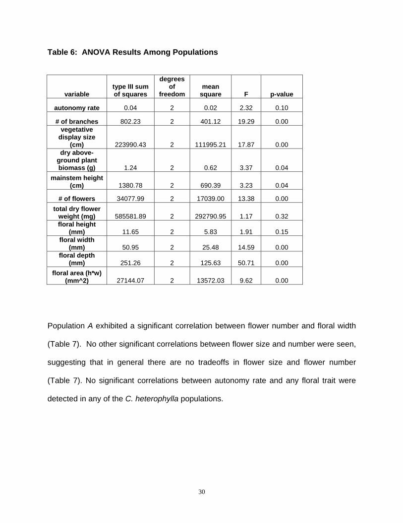
Table 6: ANOVA Results Among Populations
variable type III sum of squares
degrees of
freedom mean
square F p-value
autonomy rate 0.04 2 0.02 2.32 0.10
# of branches 802.23 2 401.12 19.29 0.00 vegetative
display size (cm) 223990.43 2 111995.21 17.87 0.00
dry above-ground plant biomass (g) 1.24 2 0.62 3.37 0.04
mainstem height (cm) 1380.78 2 690.39 3.23 0.04
# of flowers 34077.99 2 17039.00 13.38 0.00 total dry flower
weight (mg) 585581.89 2 292790.95 1.17 0.32 floral height
(mm) 11.65 2 5.83 1.91 0.15 floral width
(mm) 50.95 2 25.48 14.59 0.00 floral depth
(mm) 251.26 2 125.63 50.71 0.00 floral area (h*w)
(mm^2) 27144.07 2 13572.03 9.62 0.00
Population A exhibited a significant correlation between flower number and floral width
(Table 7). No other significant correlations between flower size and number were seen,
suggesting that in general there are no tradeoffs in flower size and flower number
(Table 7). No significant correlations between autonomy rate and any floral trait were
detected in any of the C. heterophylla populations.
30

Table 7: Correlation Coefficients Among Populations of C. heterophylla. Pearson’s correlation results above the diagonal, and Spearman’s correlation results below the diagonal. All correlations of autonomy rate and floral measures were non-significant (p>0.05). Sample sizes are noted in Table 1. * p<0.05, ** p<0.01
C. heterophylla
A autonomy
rate flower
number
Average floral depth
average floral
height
average floral width
average floral area
total dry floral
weight
autonomy rate 1
-0.179 (0.424)
-0.235 (0.293)
0.074 0.742
-0.327 (0.138)
-0.225 (0.315)
-0.439* (0.46)
flower number
-0.061 (0.786) 1
0.077 (0.733)
0.120 (0.596)
-0.040 (0.861)
0.046 (0.840)
0.549** (0.010)
average floral depth
-0.188 (0.402)
0.205 (0.360) 1
0.247 (0.233)
0.819** (0.000)
0.799** (0.000)
0.701** (0.000)
average floral height
0.128 (0.570)
0.113 (0.617)
0.228 (0.273) 1
0.081 (0.701)
0.612** (0.001)
0.172 (0.443)
average floral width
-0.319 (0.148)
0.118 (0.601)
0.808** (0.000)
0.125 (0.553) 1
0.836** (0.000)
0.540** (0.010)
average floral area
-0.166 (0.461)
0.057 (0.801)
0.771** (0.000)
0.606** (0.001)
0.818** (0.000) 1
0.541** (0.009)
total dry floral weight
-0.389 (0.082)
0.448* (0.042)
0.740** (0.000)
0.203 (0.366)
0.600** (0.003)
0.658** (0.001) 1
31

Table 7 continued
C. heterophylla
B autonomy
rate flower
number
Average floral depth
average floral
height
average floral width
average floral area
total dry floral
weight
autonomy rate 1
0.166 (0.522)
-0.058 (0.751)
-0.189 (0.292)
0.066 (0.717)
-0.087 (0.632)
-0.001 (0.994)
flower number
0.145 (0.421) 1
0.012 (0.949)
0.019 (0.915)
-0.463** (0.007)
-0.206 (0.250)
0.884** (0.000)
average floral depth
-0.085 (0.637)
-0.082 (0.649) 1
0.398* (0.018)
0.143 (0.411)
0.356* (0.036)
0.249 (0.162)
average floral height
-0.100 (0.579)
0.057 (0.751)
0.320 (0.061) 1
0.394* (0.019)
0.884** (0.000)
0.129 (0.473)
average floral width
0.107 (0.503)
-0.402* (0.020)
0.227 (0.189)
0.372* (0.028) 1
0.775** (0.000)
-0.361* (0.039)
average floral area
-0.001 (0.994)
-0.196 (0.275)
0.318 (0.063)
0.793** (0.000)
0.834** (0.000) 1
-0.083 (0.645)
total dry floral weight
-0.041 (0.821)
0.907** (0.000)
0.124 (0.493)
0.109 (0.546)
-0.342 (0.052)
-0.123 (0.496) 1
C. heterophylla
C autonomy
rate flower
number
Average floral depth
average floral
height
average floral width
average floral area
total dry floral
weight
autonomy rate 1
-0.022 (0.890)
0.040 (0.809)
-0.097 (0.556)
-0.277 (0.088)
-0.233 (0.154)
-0.011 (0.946)
flower number
-0.073 (0.656) 1
-0.125 (0.449)
-0.114 (0.488)
-0.040 (0.810)
-0.109 (0.509)
0.864** (0.000)
average floral depth
-0.051 (0.758)
-0.063 (0.704) 1
0.282 (0.078)
0.119 (0.466)
0.283 (0.077)
0.072 (0.667)
average floral height
-0.099 (0.547)
-0.118 (0.474)
0.276 (0.085) 1
0.141 (0.386)
0.827** (0.000)
0.075 (0.654)
average floral width
-0.289 (0.075)
-0.035 (0.832)
0.080 (0.622)
0.159 (0.327) 1
0.669** (0.000)
0.086 (0.608)
average floral area
-0.231 (0.156)
-0.130 (0.429)
0.264 (0.100)
0.844** (0.000)
0.623** (0.000) 1
0.096 (0.567)
total dry floral weight
0.001 (0.993)
0.901** (0.000)
0.169 (0.312)
0.076 (0.651)
0.094 (0.574)
0.062 (0.712) 1
32

Discussion
Among-species scaling in the genus Collinsia: Species within the genus Collinsia
exhibit a wide range of floral sizes (6-16 mm Figure 1). While there is a general positive
relationship between flower and plant height within the genus (Figure 4), many species
do not conform to this relationship. The vegetatively-largest species have, in general,
large flowers, and the vegetatively smallest species vary significantly in flower size
(Figures 4). Surprisingly, the two species with the smallest vegetative size are both the
largest and smallest flowered species in the genus (C. corymbosa and C. torreyi
wrightii, respectively). This variation is also reflected in the dramatic changes in rank
order of plant size and flower size (Figure 3).
The allometric scaling approach used here accounts for variation in plant size among
related species when considering variation in floral size. The regression of average
floral height on average plant height explained 20% of the variation among these
species, indicating that deviation from the general scaling relationship within Collinsia is
common. The degree and direction of deviation from the general scaling relationship
can suggest differences in the selective environment in nature that affect flower size.
Species that fall in the upper left quadrant of Figure 4 (C. corymbosa, C. greenei, C.
bartisiifolia var. bartisiifolia) have larger flowers than expected by the allometric scaling
relationship. This suggests that these species are allocating more resources than
expected to the floral traits associated with pollinator attraction (corolla size). For
example, C. corymbosa has the largest floral size and the second smallest plant size of
all the Collinsia species. Interestingly, C. corymbosa lives on the nutrient poor sand
33

dunes of Monterey County, California, where it is endemic. The over-allocation to
flower size seen in this species suggests that large flowers are favored even though
they are expected to be costly, likely because they increase pollinator attraction and
may increase outcross pollen receipt.
In contrast, species that fall in the lower left quadrant of Figure 4 have significantly
smaller flowers than expected. These include C. torreyii var wrightii, C. parviflora, C.
rattanii, and C. sparsiflora var sparsiflora. These species are expected to have been
under selection to reduce floral size and are likely highly selfing. Collinsia rattanii is
found in open coniferous forests in northwestern USA while C. parviflora is found on
rock-outcrops, grassy slopes, and beaches from California north to British Columbia and
east to Ontario (Parachnowitsch and Elle 2004) as well as moist shady places in the
mountains (Neese 1993). Elle and Carney (2003) showed that while pollinators do
occasionally visit C. parviflora, they preferentially visit large-flowered individuals within
populations and larger-flowered populations over smaller flowered populations.
Collinsia parviflora has been shown to have high autonomous selfing rates and small-
flowered individuals produce significantly more seeds through self-fertilization in a
natural pollination environment than larger-flowered individuals (Elle 2004).
Surprisingly there are no species that fall in the lower right quadrant, and few that fall
significantly above the regression line in the upper right quadrant. In fact, the amount of
variation around the regression line significantly decreases as plant size increases,
suggesting either a genetic constraint on the production of larger or smaller flowers on
large plants, or that there has been no selection to produce large plants with smaller
flowers, or large plants with very large flowers. One explanation for this low variation at
34

large plant size may be that species that inhabit productive environments can acquire
enough resources to produce large plant sizes, and are not likely to experience
selection pressure to reduce floral costs. Species that inhabit highly productive
environments with pollinator variability or failure may not be selected to reduce floral
size, but may instead be selected to change the timing of selfing via reduced
herkogamy and dichogamy to ensure reproductive success. The reduced variability in
floral size in the species with the largest plant sizes may also indicate an optimum in
floral size for larger plants.
No clear predictions can be made about the mating system of species that fall along
the regression line except that small flowered species are likely to be more selfing while
large flowered species are likely to be more outcrossing. For example, C. verna, with an
average floral height of 15 mm is among the largest flowers in the genus. This species
exhibits a delayed selfing mating system where flowers are able to outcross first, but
reduce herkogamy late in floral life to enable self-fertilization (Kalisz et al 1999.) In this
manner, ovules that are not outcross-fertilized can be self-fertilized yielding a mixed
mating system. Collinsia verna experiences pollinator variability within and among
seasons (Kalisz and Vogler 2003), and expresses a mixed mating system with
outcrossing rates dependent on pollinator visitation rates (t ranges from 0.62 to 1.0;
Kalisz and Vogler 2003; Kalisz et al 2004). Likewise, C. heterophylla, also among the
largest flowered species, has been shown to expressa range of outcrossing rates (t
ranges from 0.32 to 0.64; Mayer, et al 1996).
The availability of a phylogeny for the tribe Collinsieae (Armbruster et al 2002) and
the use of allometric scaling and the comparative method allow for several interesting
35

patterns to be explored. First, there are three species whose subspecies fall both
above, on, and/or below the line (Figure 4) (C. sparsiflora, C. torreyi, and C. bartsiifolia).
In the subspecies of C. sparsiflora all have similar average plant height, but express
large variation in floral size - one subspecies falls above (C. sparsiflora arvensis 17
mm), one falls along (C. sparsiflora collina 10 mm), and one falls below (C. sparsiflora
sparsiflora 7mm) the regression line. These three subspecies are likely experiencing
different selection pressures on floral size and may be evolving toward different mating
systems. Sparsiflora arvensis inhabits dry meadows, old fields, and rocky grass slopes
(Neese 1993) and may experience an environment in which pollinators are more
abundant and more dependable and may be under selection pressure to increase floral
size and outcrossing rate. In contrast, C. sparsiflora sparsiflora is generally found in
grassy disturbed areas and in chaparral (Neese 1993) and may experience an
environment in which pollinators are rare or unpredictable and experience selection
pressure to reduce floral size and to increase autonomy ability to ensure that offspring
are produced (reproductive assurance). Collinsia sparsiflora collina is found in a wider
range of disturbed habitats including roadsides, grassy fields, open chaparral, and
foothill wetlands (Neese 1993). This variety of environments may favor delayed selfing.
In contrast, the four subspecies of C. torreyi all have similar plant sizes, but one of the
four (C. torreyi wrightii) has a significantly smaller average flower size (5 mm) than the
others (7.5mm) (Neese 1993). Collinsia torreyi wrightii inhabits the highest elevations of
all the subspecies and the change in allometric scaling may parallel a change in mating
system in response to low pollination and resource conditions related to a short growing
season. The styles of the smaller flowered C. torreyi wrightii and C. sparsiflora
36

sparsiflora come into contact with self-pollen earlier in floral development than the larger
flowered subspecies (Armbruster et al 2002) further supporting the hypothesis that the
smaller subspecies may be evolving towards a more selfing mating system.
Allometric scaling within and among four species of Collinsia: A closer look at the
scaling relationships within species from my greenhouse experiment (Figures 6 and 6)
reveals individual variation not possible to see in the among-species level analyses
(Figure 4). The scaling coefficients (k) differ among species analyzed, and the k
coefficients for the species differ from that calculated for genus overall suggesting
evolutionary divergence among species. While species overall occupied different areas
of the scaling graph (Figures 6a, b), individuals overlap among species. Since,
individuals in this experiment were grown under identical greenhouse conditions, this
suggests that they differ genetically in their individual responses to the growth
environment. Individual variation in plant height and floral height for C. verna, C.
heterophylla A, and C. heterophylla C was extreme and the regression was not
significant for any of these species.
Variation in floral size within and among species of Collinsia: Many factors can
cause flower size to become smaller, including resource limitation (Holtsford and
Ellstrand 1992; Diggle 1997; Elle and Hare 2002; Case and Barrett 2004) and pollinator
limitation (Elle and Carney 2003) or flower size to become larger, such as increased
pollinator attraction and/or competition for pollinators (Conner and Rush 1996; Totland
2001). In both the among and within species comparisons, the choice of variables to
37

represent flower size led to very different scaling relationships and different patterns of
species variation (Figures 6ab, 6ab). For example, in my ANOVA analyses, I found no
difference among populations of C. heterophylla in floral height, but significant
differences were found in floral width, depth, and area (Table 4). When I used floral
area (height *width of the corolla) instead of floral height in my regressions, I marginally
increased the variation explained for C. heterophylla B from 10% to 13%. Since no
single measurement was found to be used consistently in the literature, several
variables were measured in this study for both plant and flower size. Correlation
analyses among these variables showed no consistent pattern among species or
populations. In C. tinctoria and C. verna there were significant correlations among the
floral size measures (Table 5), but C. heterophylla varied in its correlations for each of
the different populations (Table 7). Significant correlations of flower size to total dry
floral weight were found in C. tinctoria, but not in the other species studied. The amount
of variation in floral trait estimation, and in the correlations among traits, makes it
difficult to determine the ‘best’ measures to use in these analyses. My results suggest
that the choice of variables in allometric scaling studies can affect the results and that
multiple measurements should be taken to fully understand scaling patterns.
Floral height is less variable than plant height (Figure 5), and has a lower coefficient
of variation (CV) across all species. This suggests that natural selection may be acting
differently on the two variables- maintaining floral size while allowing plant size to vary
with environmental conditions. Previous field estimates of average plant (main stem)
height in C. heterophylla varied from 210 to 270 mm (Weil and Allard 1967). My
greenhouse estimates of height for C. heterophylla ranged from 310-355 mm (Block 1)
38

to 575 to 665 mm (Block 2) suggesting that plant height is indeed a flexible character
and can vary with changing environmental conditions.
Collinsia heterophylla and C. tinctoria are among the largest-flowered species in the
genus, (Figure 1) and there is clearly more variation in floral size for the larger-flowered
species than for the smaller-flowered species. Interestingly, some species were so
variable in floral size despite constant plant size that they have been differentiated into
varieties (C. sparsiflora, C. bartsiifolia, and C. torreyi) (Neese 1993).
When I compare the results of this study to previous work on Collinsia, I find that
estimates of floral size in C. heterophylla are more variable among populations than
within populations. This might indicate stabilizing selection within populations, but
divergence among populations. Previous C. heterophylla estimates of average corolla
lobe width varied from 5-6 mm and average corolla lobe length varied from 7.6-10.6 mm
(Charlesworth and Mayer 1995). My estimates of C. heterophylla average corolla
height varied between 16.7 and 17.6 mm and average corolla width averaged 13-14.5
mm. In block 1, where temperatures were significantly higher, average floral height
ranged from 14-15 mm and width ranged from 10-12 mm. While block 1 estimates are
smaller than block 2 estimates, both blocks are larger than previous reports. There
were no significant correlations between flower size and flower number in any of the
species investigated here, suggesting there is no tradeoff in allocation to size versus
number.
Autonomy ability (= the production of fruits via autonomous self pollination) is also
variable within and among these species. Populations of C. heterophylla autonomy
rates averaged 0.10 to 0.16 while individuals varied from 0 to 0.5. Since all plants were
39

grown in greenhouse conditions with regular water and fertilizer, they should not have
been resource limited. Collinsia heterophylla is found throughout California (Neese
1993) and populations appear to vary significantly in their ability to autonomously self-
fertilize (Armbruster et al 2002). This level of variation is found in other species as well,
and may not be simply described by population level differences. In one study of C.
verna, average autonomy rates were estimated at 0.33, with individual estimates
varying from 0 to 0.8. In a second study, C. verna populations were estimated to have
average autonomy rates of 0.5 with individual estimates varying from 0 to 1.0 (Kalisz
and Vogler 2003). The average autonomy rate estimated here for C. verna was lower
(0.15) and individuals varying from 0 to 0.35. One explanation for the difference is that
previous studies were done in exclosures under field conditions, while this study was
conducted under greenhouse conditions. It is possible that wind may facilitate within
flower selfing. It is also possible that given the degree of individual variation in
autonomy ability, that my estimates may simply be a result of sampling.
In C. tinctoria, autonomy rate was significantly positively correlated with all measures
of individual flower size (floral height, width, depth, and area; Table 5) suggesting that
floral size and shape are important factors in the ability of individual flowers to produce
seeds autonomously. It is possible that either herkogamy and/or dichogamy are
influencing the low average selfing ability in this species, and that changes in floral size
and shape may enable self-fertilization among some individuals. In contrast, autonomy
rate in C. verna was significantly correlated with the total number of flowers on a plant
as well as the total dry floral biomass (Table 5). In this species, autonomy ability is not
40
correlated to size and shape variables, but instead is correlated to the total number and
weight of flowers.
Conclusions
The genus Collinsia is variable within and among species in morphological
characteristics related to flower size and plant size. The degree and direction of
variation from the general allometric scaling pattern can be used to further examine this
variation and to generate hypotheses concerning the selective environments that may
be influencing the observed variation. Scaling relationship for flower size and plant size
differ at the genus, species, and population level and, in some cases, are non-
significant. In addition to floral size, autonomy ability was found to vary. Both the
phylogenetic history and the selective environment will have a significant effect on
deviations from the allometric relationships of a population or species and may affect
the mating system expressed. Additional work is in progress to further understand the
forces generating variation within this genus and to understand the potential role of
mating system flexibility in the evolution of species.
41

BIBLIOGRAPHY Andersson, S. 2005. Floral costs in Nigella sativa (Ranunculaceae): Compensatory
responses to perianth removal. American Journal of Botany 92(2): 279-283. Armbruster, W.S., Di Stilio VS, Tuxill JD, Flores TC, Runk JLV. 1999. Covariance and
decoupling of floral and vegetative traits in nine neotropical plants: A re-evaluation of Berg's correlation-pleiades concept. American Journal of Botany 86 (1): 39-55.
Armbruster, W.S., Mulder, C.P.H., Baldwin, B.G., Kalisz, S., Wessa, B., and Nute, H.
2002. Comparative Analysis of Late Floral Development and Mating-System Evolution in the Tribe Collinsieae (Scrophulariaceae SL). American Journal of Botany 89(1): 37-49.
Arthur, W. 2003. Developmental Constraint and Natural Selection. Evolution & Development 5(2): 117-118.
Ashman, TL and Schoen, D.J. 1997. The Cost of Floral Longevity in Clarkia tembloriensis: An Experimental Investigation. Evolutionary Ecology 11(3): 289-300.
Baker, H.G. 1955. Self-Compatibility and Establishment After “Long-Distance” Dispersal. Evolution 9: 347-348.
Barrett, S.C.H. 2002. The Evolution of Plant Sexual Diversity. Nature Reviews Genetics 3(4) 274-284.
Barrett, SCH. 2003. Mating Strategies in Flowering Plants: The Outcrossing-Selfing Paradigm and Beyond. Philosophical Transactions of the Royal Society of London B- Biological Sciences 358(1434): 991-1004.
Byers, D.L. and Waller, D.M. 1999. Do Plant Populations Purge Their Genetic Load?
Effects of Population Size and Mating History on Inbreeding Depression. Ann.Rev.Ecol.Syst.30:479-513.
Carr DE, Dudash MR. 2003. Recent Approaches into the Genetic Basis of Inbreeding Depression in Plants. Philosophical Transactions of the Royal Society of London Series B- Biological Sciences 358 (1434): 1071-1084.
42

Case, A.L. and Barrett, S.C.H. 2004. Environmental stress and the evolution of dioecy: Wurmbea dioica (Colchicaceae) in Western Australia. Evolutionary Ecology 18(2): 145-164.
Charlesworth, D and Charlesworth, B. 1987. Inbreeding Depression and its Evolutionary
Consequences. Ann. Rev. Ecol. Syst. 18: 237-268.
Charlesworth, D. and Charlesworth, B. 1995. Quantative Genetics in Plants: The Effect of the Breeding System on Genetic Variability. Evolution 49(5): 911-920.
Charlesworth, D. and Mayer, S.1995. Genetic Variability of Plant Characters in the
Partial Inbreeder Collinsia heterophylla (Scrophulariaceae). American Journal of Botany 82(1): 112-120.
Cheptou P.O. and Dieckmann, U. 2002. The Evolution of Self-Fertilization in Density-
Regulated Populations. Proceedings of the Royal Society of London Series B- Biological Sciences 269 (1496): 1177-1186
Connor, J.K., and Rush, S. 1996. Effects of Flower Size on Pollinator Visitation to Wild Radish, Raphanus raphanistrum. Oecologia 105(4): 509-516.
Cresswell, J.E. and Galen C. 1991. Frequency-dependent Selection and Adaptive
Surfaces for Floral Character Combinations: The Pollination of Polemonium viscosum. The American Naturalist 138 (6): 1342-1353.
Diggle, P.K. 1997. Ontogenetic contingency and floral morphology: The effects of
architecture and resource limitation. International Journal of Plant Sciences 158(6) Supplemental S: S99-S107.
Donnelly, S.E., Lortie, C.J., and Aarssen, L.W. 1998. Pollination in Verbascum thapsus
(Scrophulariaceae): The Advantage of Being Tall. American Journal of Botany 85(11) 1618-1625.
Elle, E and Hare, J.D. 2002. Environmentally Induced Variation in Floral Traits Affects
the Mating System in Datura wrightii. Functional Ecology 16(1): 79-88. Elle, E. and Carney, R. 2003. Reproductive Assurance Varies with Flower Size in
Collinsia parviflora (Scrophulariaceae). Am. J. Bot. 90(6): 888-896. Elle, E. 2004. Floral Adaptations and Biotic and Abiotic Selection Pressures. In
Q.C.B. Cronk, J. Whitton, R.H. Ree, and I.E.P.Taylor [eds], Plant Adaptation: Molecular Genetics and Ecology. Proceedings of and International Workshop held December 11-13, 2002, in Vancouver, British Columbia, Canada. NRC Research Press, Ottawa, Ontario, Canada.
43

Fausto, J.A., Eckhart, V.M., and Gerber, M.A. 2001. Reproductive Assurance and the Evolutionary Ecology of Self-Pollination in Clarkia xantiana (Onagraceae). American Journal of Botany 88: 1794-1800.
Fenster, Charles B. and Ritland, Kermit. 1994. Evidence for Natural Selection on Mating
System in Mimulus (Scrophulariaceae). Int. J. Plant Science 155(5). pp 588-596.
Fisher, R.A. 1941. Average Excess and Average Effect of a Gene Substitution. Annals
of Eugenics 11:53-63. Frey, F.M. 2004. Opposing natural selection from herbivores and pathogens may
maintain floral-color variation in Claytonia virginica (Portulacaceae). Evolution 58(11): 2426-2437.
Galen, C. 1989. Measuring Pollinator-Mediated Selection on Morphometric Floral
Traits: Bumble Bees and the Alpine Sky Pilot, Polemonium viscosum. Evolution 43: 882-890.
Galen, C. 1996. Rates of Floral Evolution: Adaptation to Bumble Bee Pollination
in an Alpine Wildflower, Polemonium viscosum. Evolution 50(1): 120-125. Galen, C. 1999. Why do Flowers Vary? The Functional Ecology of Variation in Flower
Size and form Within Natural Plant Populations. Bioscience 49(8): 631-640. Galen, C. 2000. High and Dry: Drought Stress, Sex-Allocation Trade-offs, and Selection
on Flower Size in the Alpine Wildflower Polemonium viscosum (Polemoniaceae). Am. Nat. 156 (1): 72-83.
Garber, E.D. 1975. Collinsia. in R.C.King (ed). Handbook of Genetics Vol II: Plants,
Plant Viruses, and Protists. Plenum. New York. Gayon, Jean. 2000. History of the Concept of Allometry. Amer Zool. 40: 748-758.
Gray, Asa (1810-1888). 1970. Gray's Manual of botany: a handbook of the
flowering plants and ferns of the central and northeastern United States and adjacent Canada. 8th (Centennial) ed., ill. / largely rewritten and expanded by Merritt Lyndon Fernald, with assistance of specialists in some groups, Corr. print., 1970 / corrections supplied by R.C. Rollins. New York: D. Van Nostrand Co.
Harder, L.D. and Wilson, W.G. 1998. A Clarification of Pollen Discounting and its Joint
Effects With Inbreeding Depression on Mating System Evolution. American Naturalist 152 (5): 684-695.
44

Herlihy, C.R. and Eckert, C.G. 2002. Genetic Costs of Reproductive Assurance in a Self-Fertilizing Plant. Nature 416: 320-323.
Herrera J. 2001. The Variability of Organs Differentially Involved in Pollination, and
Correlations of Traits in Genisteae (Leguminosae: Papilionoideae) Herrera, C.M., Sanchez-Lafuente, A.M., Medrano, M., Guitian, J., Xim, C., and Rey, P.
2001. Geographical Variation in Autonomous Self-Pollination Levels Unrelated to Pollinator Service in Helleborus foetidus (Ranunculaceae). Am. J. Bot. 88(6): 1025-1032.
Herrera, J. 2004. Lifetime Fecundity and Floral Variation in Tuberaria guttata
(Cistaceae), a Mediterranean Annual. Plant Ecology 172: 219-225. Herrera, J. 2005. Floral Size Variation in Rosmarinus officinalis: Individuals, Populations
and Habitats. Annals of Botany 95: 431-437. Holsinger, K.E., Feldman, M.W., and Christiansen, F.B. 1984. The Evolution of Self-
Fertilization in Plants: A Population Genetic Model. Am. Nat. 138: 446-453. Holsinger, K.E. 1986. Dispersal and Plant Mating Systems: The Evolution of Self-
Fertilization in Subdivided Populations. Evolution 40: 405-413. Holsinger, K.E. 1988. Inbreeding Depression Doesn’t Matter: The Genetic Basis of
Mating-System Evolution. Evolution 42: 1235-1244. Holsinger, K.E. 1991. Mass-Action Models of Plant Mating Systems: The Evolutionary
Stability of Mixed Mating Systems. Am. Nat. 138: 606- 622. Holsinger, K.E. 1992a. Ecological Models of Plant Mating Systems, pp 169-191 in
Ecology and Evolution of Plant Reproductive System, edited by R.W. Wyatt. Chapman and Hall, New York.
Holsinger, Kent. 1992b. Commentary: Functional Aspects of Mating System Evolution in Plants. Int. J. of Plant Sciences. 153(3) iii-v.
Holsinger, K.E. 1996. Pollination Biology and the Evolution of Mating Systems in
Flowering Plants. Evol. Biol. 29: 107-149. Holsinger, Kent. 2000. Reproductive Systems and Evolution in Vascular Plants.
PNAS. Vol 97 number 13 pp.7037-7042. Holtsford, T.P. and Ellstrand, N.C. 1992. Genetic and Environmental Variation in
Floral Traits Affecting Outcrossing Rate in Clarkia tembloriensis (Onagraceae). Evolution 46(1) 216-225.
45

Jarne, P and Charlesworth, D. 1993. The Evolution of Selfing Rate in Functionally Hermaphroditic Plants and Animals. Ann. Rev. Ecol. Syst. 24: 441-466.
Johnston, M.O. 1998. Evolution of Intermediate Selfing Rates in Plants:
Pollination Ecology vs. Deleterious Mutations. Genetica 102-103: 267-278 special issue SI 1998.
Kalisz, S., Vogler, D., Fails, B., Finer, M., Shepard, E., Herman, T., and Gonzales, R.
1999. The mechanism of Delayed Selfing in Collinsia verna (Scrophulariaceae). American Journal of Botany 86(9): 1239-1247.
Kalisz, S. and Vogler, D.W. 2003. Benefits of Autonomous Selfing Under Unpredictable Pollinator Environments. Ecology 84(11): 2928-2942.
Kalisz, S., Vogler, D.W., and Hanley, K. 2004. Context-Dependent Autonomous Self- Fertilization Yields Reproductive Assurance and Mixed Mating. Nature (430:7002): 884-887.
Knudsen, J.T. 1994. Floral Scent Variation in the Pyrola-Rotundifolia Complex in
Scandinavia and Western Greenland. Nordic Journal of Botany 14 (3): 277-282. Lande, R, and Schemske D.W. 1985. The Evolution of Self-Fertilization and Inbreeding
Depression in Plants. I. Genetic Models. Evolution 39(1) pp. 24-40. Lloyd, D. 1979. Some Reproductive Factors Affecting the Selection of Self -Fertilization
in Plants. American Naturalist 113: 67-69. Lloyd, D. 1992. Self- and Cross-Fertilization in Plants. II. The Selection of Self-
Fertilization. Int. J. Plant Sci. 153(3) pp 370-380. Lloyd, D.G. and Schoen, D.J. 1992. Self- and Cross-Fertilization in Plants. I. Functional
Dimensions. Int. J. Plant Sci. 153(3) pp 358-369. Mayer, S.S., Charlesworth, D., Meyers, B. 1996. Inbreeding Depression in Four
Populations of Collinsia heterophylla Nutt (Scrophulariaceae). Evolution 50(2): 879-891.
Moody, M.L. and Hufford, L. 2000. Floral ontogeny and morphology of Cevallia,
Fuertesia, and Gronovia (Loasaceae subfamily Gronovioideae). International Journal of Plant Sciences 161(6): 869-883.
Neese, E.C. 1993. Collinsia. Pp 1024-1027 in J.C. Hickman (ed), The Jepson
Manual. Higher Plants of California. University of California Press, Berkeley, California, USA
46

Niklas, Karl. 1994. Plant Allometry: The Scaling of Form and Process. Chicago. University of Chicago Press.
Niklas, K. 2004. Plant Allometry: is there a grand unifying theory? Biol. Rev. (79): 871-
889. Parachnowitsch, A.L. and Elle, E. 2004. Variation in Sex Allocation and Male-Female
Trade-offs in Six Populations of Collinsia parviflora (Scrophulariaceae S.L.). American Journal of Botany 91(8): 1200-1207.
Sakai, S. 1995. Evolutionary Stable Selfing Rates of Hermaphroditic Plants in
Competing and Delayed Selfing Modes with Allocation to Attractive Structures. Evolution 49: 557-564.
Sakai, S. and Ishii, H.S. 1999. Why be Completely Outcrossing? Evolutionarily Stable
Outcrossing Strategies in an Environment Where Outcross-Pollen Availability is Unpredictable. Evolutionary Ecology Research 1(2): 212-222.
Sanchez-Lafuente, A.M. 2002. Floral Variation in the Generalist Perennial Herb
Paeonia broteroi (Paeoniaceae): Differences Between Regions with Different Pollinators and Herbivores. Am. J. Bot. 89(8): 1260-1269.
Schemske, D.W. and Lande, R. 1985. The Evolution of Self-Fertilization and Inbreeding Depression in Plants. II. Empirical Observations. Evolution 39: 41-52.
Schemske, D.W. and Bradshaw Jr., H.D. 1999. Pollinator Preference and the Evolution
of Floral Traits in Monkeyflowers (Mimulus). PNAS 96(21): 11910-11915.
Schoen, D.J. and Brown, AHD. 1991. Whole- and Part-Flower Self-Pollination in Glycine clandestina and G. aryrea and the Evolution of Autogomy. Evolution 45: 1651-1664.
Takebayashi, N. and Morrell, P.L. 2001. Is Self-Fertilization an Evolutionary Dead End?
Revisiting an Old Hypothesis with Genetic Theories and A Macroevolutionary Approach. American Journal of Botany 88(7). Pp 1143-1150.
Totland, O. 2001. Environment-dependent pollen limitation and selection on floral traits
in an alpine species. Ecology 82(8): 2233-2244. Tsitrone A, Duperron S, David P. 2003. Delayed Selfing as an Optimal Mating Strategy
in Preferentially Outcrossing Species: Theoretical Analysis of the Optimal Age at First Reproduction in Relation to Mate Availability. American Naturalist 162(3):318-331.
Uyenoyama, M.K. 1986. Inbreeding and the Cost of Meiosis: The Evolution of Selfing in Populations Practicing Biparental Inbreeding. Evolution 40:399-404.
47

Uyenoyama, M.K., and Waller, D. M. 1991. Coevolution of Self-Fertilization and
Inbreeding Depression. I. Mutation-Selection Balance at One and Two Loci. Theor. Population Biology 40: 14-46.
Uyenoyama, M.K., Holsinger, K.E., and Waller, D.M. 1993. Ecological and Genetic Factors Directing the Evolution of Self-Fertilization. Oxford Surv. Evol. Bio. 9:327-381.
Ushimaru, A. and Nakata, K. 2001. Evolution of Flower Allometry and its Significance
for Pollination Success in the Deceptive Orchid Pogonia japonica. Int. J. Plant. Sci. 162(6): 1307-1311.
Ushimaru, A. and Nakata, K. 2002. The Evolution of Flower Allometry in Selfing
Species. Evolutionary Ecology Research 4:1217-1227. Vogler, Donna, and Kalisz, Susan. 2001. Sex Among the Flowers: The Distribution of
Plant Mating Systems. Evolution 55(1) pp 202-204.
West, G.B., Brown, J.H., and Enquist, B.J. 1997. A general model for the origin of allometric scaling laws in biology. Science (276): 122-126.
West, G.B., Brown, J.H., and Enquist, B.J. 1999. The fourth dimension of life: fractal
geometry and allometric scaling of organisms. Science (284): 167-169. West, G.B., Brown, J.H., and Enquist B.J. 2000.The origin of universal scaling laws in
biology. In Scaling in Biology (eds. J.H. Brown and G.W. West). pp 87-112. Oxford University Press, NY
Yahara, T. 1992. Graphical Analysis of Mating system Evolution in Plants. Evolution
46(2): 557-561.
48