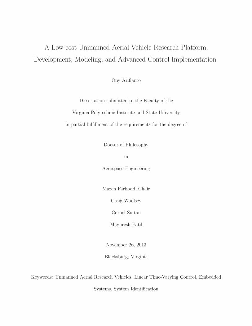
A Low-cost Unmanned Aerial Vehicle Research Platform:

Development, Modeling, and Advanced Control Implementation

Ony Arifianto

Dissertation submitted to the Faculty of the

Virginia Polytechnic Institute and State University

in partial fulfillment of the requirements for the degree of

Doctor of Philosophy

in

Aerospace Engineering

Mazen Farhood, Chair

Craig Woolsey

Cornel Sultan

Mayuresh Patil

November 26, 2013

Blacksburg, Virginia

Keywords: Unmanned Aerial Research Vehicles, Linear Time-Varying Control, Embedded

Systems, System Identification

A Low-cost Unmanned Aerial Vehicle Research Platform:

Development, Modeling, and Advanced Control Implementation

Ony Arifianto

(ABSTRACT)

This dissertation describes the development and modeling of a low-cost, open source, and

reliable small fixed-wing unmanned aerial vehicle (UAV) for advanced control implemen-

tation. The platform is mostly constructed of low-cost commercial off-the-shelf (COTS)

components. The only non-COTS components are the airdata probes which are manufac-

tured and calibrated in-house, following a procedure provided herein. The airframe used is

the commercially available radio-controlled 6-foot Telemaster airplane from Hobby Express.

The airplane is chosen mainly for its adequately spacious fuselage and for being reasonably

stable and sufficiently agile. One noteworthy feature of this platform is the use of two sepa-

rate low-cost open source onboard computers for handling the data management/hardware

interfacing and control computation. Specifically, the single board computer, Gumstix Overo

Fire, is used to execute the control algorithms, whereas the autopilot, Ardupilot Mega, is

mostly used to interface the Overo computer with the sensors and actuators. The platform

supports multi-vehicle operations through the use of a radio modem that enables multi-point

communications.

As the goal of the development of this platform is to implement rigorous control algorithms for

real-time trajectory tracking and distributed control, it is important to derive an appropriate

flight dynamic model of the platform, based on which the controllers will be synthesized. For

that matter, reasonably accurate models of the vehicle, servo motors and propulsion system

are developed. Namely, the output error method is used to estimate the longitudinal and

lateral-directional aerodynamic parameters from flight test data. The moments of inertia

of the platform are determined using the simple pendulum test method, and the frequency

response of each servomotor is also obtained experimentally. The Javaprop applet is used to

obtain lookup tables relating airspeed to propeller thrust at constant throttle settings.

Control systems are also designed for the regulation of this UAV along real-time trajecto-

ries. The reference trajectories are generated in real-time from a library of pre-specified

motion primitives and hence are not known a priori. Two concatenated primitive trajecto-

ries are considered: one formed from seven primitives exhibiting a figure-8 geometric path

and another composed of a Split-S maneuver that settles into a level-turn trim trajectory.

Switched control systems stemming from ℓ2-induced norm synthesis approaches are designed

for discrete-time linearized models of the nonlinear UAV system. These controllers are ana-

lyzed based on simulations in a realistic operational environment and are further implemented

on the physical UAV. The simulations and flight tests demonstrate that switched controllers,

which take into account the effects of switching between constituent sub-controllers, man-

age to closely track the considered trajectories despite the various modeling uncertainties,

exogenous disturbances and measurement noise. These switched controllers are composed of

discrete-time linear sub-controllers designed separately for a subset of the pre-specified prim-

itives, with the uncertain initial conditions, that arise when switching between primitives,

incorporated into the control design.

iii

For my parents, wife, and kids.

iv

Acknowledgments

I would never have been able to finish this dissertation without the grace of God, guidance

from my committee members, help from friends, and support from my family and wife.

I would like to express my deepest gratitude to my Advisor, Dr. Mazen Farhood, who taught

me the value of dilligence and excellence in research. His high standard in every aspect of

his work motivated me to take the extra mile in all of the works that I had done. I would

also like to thank Dr. Craig Woolsey for helping me to build my presentation skill and

my confidence. I would like to thank Dr. Cornel Sultan and Dr. Mayuresh Patil for their

constructive feedbacks throughout the process.

I also would like to thank the Nonlinear Systems Laboratory (NSL) crew, Artur Wolek for

the sincere feedbacks, Dave Grymin for the time spent proofreading paper and dissertation

scripts, Mark Palframan for the excellent videos and pictures, Ankit Ganeriwal, Hossam

Abdelwahid, Tejasui Gode and Eddie Hale, for the help, support and friendship that made

the past five years memorable.

I would like to thank the Nuenighoff family, mas Curt, mbak Sita, Glen, Erik, and Lexi for

being great friends and providing me with a place to stay in the last few months.

I would like to thank my mom and dad for being the main reason I undertook this PhD

program, this dissertation is my gift for you.

I also would like to thank my brothers for supporting the endeavour and for taking care of

our parents while I am far away. I thank my children for being wonderful, I will make up

v

for the camps, conferences, performances and trips that I missed. For my wife, there is not

enough words to express my gratitude for your support, patience in taking care of the kids,

and toughness to be on my side through this hard time.

Finally, I would like to thank Dr.-Ing. B. J. Habibie, Dr. Ing. O. H. Gerlach, and Dr. S. D.

Jenie for being my inspiration.

vi

Contents

1 Introduction 1

1.1 Overview . . . . . . . . . . . . . . . . . . . . . . . . . . . . . . . . . . . . . . 1

1.2 Low-Cost Research Platform . . . . . . . . . . . . . . . . . . . . . . . . . . . 3

1.3 Advanced Control System Implementation . . . . . . . . . . . . . . . . . . . 6

1.4 Contributions . . . . . . . . . . . . . . . . . . . . . . . . . . . . . . . . . . . 11

1.5 Organization . . . . . . . . . . . . . . . . . . . . . . . . . . . . . . . . . . . 13

2 Aerial Research Platform Development 14

2.1 System Description and Architecture . . . . . . . . . . . . . . . . . . . . . . 14

2.2 Airdata Probe . . . . . . . . . . . . . . . . . . . . . . . . . . . . . . . . . . . 20

2.2.1 Probe design and manufacturing . . . . . . . . . . . . . . . . . . . . . 21

2.2.2 Probe calibration . . . . . . . . . . . . . . . . . . . . . . . . . . . . . 24

2.2.3 Validation and analysis . . . . . . . . . . . . . . . . . . . . . . . . . . 28

3 Mathematical Model Development 34

3.1 Aircraft Equations of Motion . . . . . . . . . . . . . . . . . . . . . . . . . . 35

3.2 Moments of Inertia . . . . . . . . . . . . . . . . . . . . . . . . . . . . . . . . 37

3.3 Servo Model . . . . . . . . . . . . . . . . . . . . . . . . . . . . . . . . . . . . 41

3.4 Propulsion Model . . . . . . . . . . . . . . . . . . . . . . . . . . . . . . . . . 44

3.5 Aerodynamic Model . . . . . . . . . . . . . . . . . . . . . . . . . . . . . . . 48

3.6 Simulation Environment . . . . . . . . . . . . . . . . . . . . . . . . . . . . . 56

4 Control System Design, Simulation, and Flight Testing 62

4.1 Preliminaries . . . . . . . . . . . . . . . . . . . . . . . . . . . . . . . . . . . 63

4.1.1 Notation . . . . . . . . . . . . . . . . . . . . . . . . . . . . . . . . . . 63

4.1.2 Control Synthesis . . . . . . . . . . . . . . . . . . . . . . . . . . . . . 64

4.1.3 Plant Model Formulation . . . . . . . . . . . . . . . . . . . . . . . . . 71

vii

4.2 Tracking of a Figure-8 Trajectory . . . . . . . . . . . . . . . . . . . . . . . . 74

4.2.1 Motion primitives . . . . . . . . . . . . . . . . . . . . . . . . . . . . . 75

4.2.2 Control design . . . . . . . . . . . . . . . . . . . . . . . . . . . . . . . 79

4.2.3 Simulation and flight test results . . . . . . . . . . . . . . . . . . . . 82

4.3 Tracking of an Aerobatic Maneuver . . . . . . . . . . . . . . . . . . . . . . . 86

4.3.1 Split-S Maneuver . . . . . . . . . . . . . . . . . . . . . . . . . . . . . 87

4.3.2 Steady Right Turn Flight . . . . . . . . . . . . . . . . . . . . . . . . 95

5 Conclusion 101

Bibliography 104

viii

List of Figures

1.1 A 6-foot Telemaster UAV and its onboard instruments . . . . . . . . . . . . 4

1.2 The plot on the left shows the UAV executing autonomously a Split-S maneu-ver followed by tracking a level-turn trim condition; the pictures on the rightare snapshots of the UAV as it performs the Split-S maneuver . . . . . . . . 6

2.1 Three UAVs interconnected over a communication network through the useof the Xbee radio modems . . . . . . . . . . . . . . . . . . . . . . . . . . . . 18

2.2 A data flow diagram of the fully programmable airborne system . . . . . . . 20

2.3 Five-hole probe and its CAD drawing . . . . . . . . . . . . . . . . . . . . . . 23

2.4 Five-hole probe calibration process . . . . . . . . . . . . . . . . . . . . . . . 24

2.5 Pressure distribution at various values of the angle of attack (α) and sideslip(β) for all ports of the probe . . . . . . . . . . . . . . . . . . . . . . . . . . . 25

2.6 Angle of attack surface fitting . . . . . . . . . . . . . . . . . . . . . . . . . . 27

2.7 Angle of sideslip surface fitting . . . . . . . . . . . . . . . . . . . . . . . . . . 28

2.8 Cp5 surface fitting . . . . . . . . . . . . . . . . . . . . . . . . . . . . . . . . . 29

2.9 Cpav surface fitting . . . . . . . . . . . . . . . . . . . . . . . . . . . . . . . . 30

2.10 Angle of attack validation at 12m/s airflow speed (left) and 20m/s speed (right) 30

2.11 Angle of sideslip validation at 12m/s airflow speed (left) and 20m/s speed(right) . . . . . . . . . . . . . . . . . . . . . . . . . . . . . . . . . . . . . . . 32

2.12 In flight measurement of the angle of attack . . . . . . . . . . . . . . . . . . 33

3.1 Moments of inertia testing setup: wire suspended cradle (left); setup to de-termine the moment of inertia about the pitch axis (top middle), the roll axis(bottom middle), and the yaw axis (right) . . . . . . . . . . . . . . . . . . . 39

ix

3.2 Test setup for the frequency domain identification of the Futaba S3152 servomodel . . . . . . . . . . . . . . . . . . . . . . . . . . . . . . . . . . . . . . . 43

3.3 Curve fitting of the servo test data . . . . . . . . . . . . . . . . . . . . . . . 44

3.4 Relationship between the throttle command δt, which is a PWM signal, andthe engine RPM . . . . . . . . . . . . . . . . . . . . . . . . . . . . . . . . . . 45

3.5 Thrust prediction as a function of airspeed and engine RPM (Javaprop) . . . 46

3.6 Test setup for measuring propeller thrust at zero airspeed . . . . . . . . . . . 47

3.7 Static thrust data along with Javaprop predictions . . . . . . . . . . . . . . . 48

3.8 Control input shapes for parameter estimation . . . . . . . . . . . . . . . . . 52

3.9 Data compatibility check using EKF prior to estimation . . . . . . . . . . . . 54

3.10 Comparison of simulated and measured responses: longitudinal parameterestimation run . . . . . . . . . . . . . . . . . . . . . . . . . . . . . . . . . . . 56

3.11 Comparison of simulated and measured responses: lateral-directional param-eter estimation run . . . . . . . . . . . . . . . . . . . . . . . . . . . . . . . . 57

3.12 Comparison of simulated and measured responses: longitudinal model valida-tion run . . . . . . . . . . . . . . . . . . . . . . . . . . . . . . . . . . . . . . 57

3.13 Comparison of simulated and measured responses: lateral-directional modelvalidation run . . . . . . . . . . . . . . . . . . . . . . . . . . . . . . . . . . . 58

3.14 Comparison of simulated and measured responses: a gentle left turn maneuver 60

3.15 Comparison of simulated and measured responses: a Split-S maneuver . . . . 61

4.1 Closed-loop system . . . . . . . . . . . . . . . . . . . . . . . . . . . . . . . . 65

4.2 Reference trajectory of a figure-8 pattern obtained by concatenating sevenmotion primitives . . . . . . . . . . . . . . . . . . . . . . . . . . . . . . . . . 78

4.3 Simulation of the controllers’ performance in forcing the nonlinear system,including the servomotors, to track the figure-8 trajectory under 2m/s steadywind, light low-altitude turbulence, one-step time delay, and measurement noise 83

4.4 Controller tracking performance in flight tests . . . . . . . . . . . . . . . . . 85

4.5 Split-S reference trajectory generation from flight test data . . . . . . . . . . 89

4.6 A representative simulation run for Split-S maneuver tracking under 3m/ssteady wind and medium turbulence . . . . . . . . . . . . . . . . . . . . . . 92

4.7 Split-S test results with penalty on position . . . . . . . . . . . . . . . . . . 93

x

4.8 Split-S test results with no penalty on position . . . . . . . . . . . . . . . . . 94

4.9 A representative simulation run for tracking of the circular trajectory under3m/s steady wind without turbulence (left plots) and with medium turbulence(right plots) . . . . . . . . . . . . . . . . . . . . . . . . . . . . . . . . . . . . 98

4.10 Flight test data showing the performance of the UIC subcontroller in trackingthe circular trajectory . . . . . . . . . . . . . . . . . . . . . . . . . . . . . . 99

4.11 Flight test results for two switched controllers designed for tracking a Split-Smaneuver that settles into a circular orbit under relatively high wind con-ditions; top plots correspond to the case where the planar position error ispenalized in the LTV subcontroller design, and bottom plots correspond tothe case where the planar position error is not penalized . . . . . . . . . . . 100

xi

List of Tables

1.1 Main geometrical parameters of the Telemaster . . . . . . . . . . . . . . . . 4

2.1 Measurement noise standard deviation (σ) . . . . . . . . . . . . . . . . . . . 17

3.1 Moments of inertia of the Telemaster UAV . . . . . . . . . . . . . . . . . . . 41

3.2 Futaba S3152 frequency response . . . . . . . . . . . . . . . . . . . . . . . . 43

3.3 Estimated measurement biases and scales . . . . . . . . . . . . . . . . . . . . 54

3.4 Estimated parameters . . . . . . . . . . . . . . . . . . . . . . . . . . . . . . 56

4.1 Trim conditions used in generating the figure-8 trajectory . . . . . . . . . . . 76

xii

Chapter 1

Introduction

1.1 Overview

The many appealing features of unmanned aerial vehicles (UAVs), such as persistence and

versatility, have rendered these systems very useful for a wide range of military, civilian, and

research applications, including real-time reconnaissance, surveillance, and target acquisi-

tion, atmospheric sciences, and disaster relief. The focus of this dissertation is miniature-

sized (less than 2 meter wing span), low-cost, but highly capable fixed-wing UAVs. Such

UAVs can be deployed in groups to perform complex and intricate tasks, and hence can

serve as a viable alternative to dispatching larger expensive high-tech aerial vehicles in cer-

tain applications. The appealing low-cost feature, which makes these UAVs expendable, is

due partly to the use of relatively cheap sensors, actuators, and processors. In addition,

1

2

the convenient small size poses restrictions on the computational and sensing capabilities.

Then, the strategy for achieving the desired high capability despite the size, weight, and

cost restrictions centers around the development of new principles and novel technologies in

software and hardware design.

Developing a UAV research platform to validate these new principles and technologies is of

great importance, and so it is no surprise that many UAV testbeds have been developed by

various academic groups, e.g., [1, 2, 3, 4, 5, 6, 7, 8, 9]. The main goal in building our testbed

is to develop a low-cost, open source, and reliable fixed-wing UAV platform that can be used

to implement relatively complex control algorithms. Building a low-cost UAV platform is not

an original idea, as other research groups in the control and robotics community have done so.

For instance, the UAV research group at the University of Minnesota have developed a low-

cost UAV testbed [1], which is mostly built of commercial-off-the-shelf (COTS) components

and uses the radio-controlled (R/C) fixed-wing UAV, Ultra Stick 25e [10], as the main test

aircraft. Another low-cost UAV platform, based on the R/C Goldberg Decathlon ARF

airframe [11], has been developed at Georgia Tech [3] for educational purposes. The UAV

research platform [8] uses the low-cost open source autopilot, Ardupilot Mega [12], and the

Aero Testbed at the University of Illinois uses the Paparazzi autopilot [13], which is also

low-cost and open source. These testbeds and others which are not mentioned here rely on

COTS components as well as hardware/software developed in-house.

3

1.2 Low-Cost Research Platform

Our testbed also consists mostly of low-cost COTS components; the only components built

in-house are the airdata probes, which are used to measure the angle of attack, sideslip, and

airspeed of the UAV. The procedure for building and calibrating these sensors is based on

[14, 15, 16] and discussed in sufficient details herein. The airframe used is the commercially

available R/C 6-foot Telemaster from Hobby Express [17]; see Figure 1.1 and Table 1.1

for the major geometric parameters of this aircraft. This aircraft is selected primarily for

its box-fuselage design, which provides ample space for onboard electronics. Furthermore,

this R/C airplane is a well-known platform that is reasonably stable, yet still capable of

performing certain aerobatic maneuvers. Minor modifications to the basic airframe were

performed in order to place sensors both in the fuselage and on the wings. Aside from

the use of standard sensors and actuators, a noteworthy feature of our platform is that

the data management/hardware interfacing and control computation are performed by two

separate onboard computers. Specifically, the low-cost open source single-board computer,

Gumstix Overo Fire [18], is used to execute the control algorithms and ultimately compute

the control commands, whereas, the COTS autopilot, Ardupilot Mega, is mostly used to

interface the Gumstix computer with the senors and actuators. The use of an XBee 900-Pro

radio modem onboard the platform allows for data transmission among multiple vehicles,

and thus the testbed also supports multi-vehicle operations.

This UAV research platform is to be used to implement systematic and rigorous approaches,

4

Figure 1.1: A 6-foot Telemaster UAV and its onboard instruments

Table 1.1: Main geometrical parameters of the Telemaster

Wing area 0.56 m2

Wing span 1.83 mWing MAC∗ 0.30 m

Mass 3.24 kg∗ MAC: mean aerodynamic chord

developed in our research lab, on controlled maneuvers, tracking along trajectories, and

distributed control, e.g., [19, 20, 21, 22, 23], and further validate formal methods for math-

ematically certified control software design. As the control design methodology pursued is

model based, it is important that we derive reasonably accurate models that capture the

rigid-body dynamics of the vehicle and any relevant subsystems. For this application, the

subsystems that directly influence the vehicle dynamics are the propulsion system and the

servos that actuate the aerodynamic control surfaces. The thrust produced by the propeller

is estimated using code that employs blade element theory [24]. Validation of the propulsion

model is performed under static test conditions. The servo motors are modeled as single-

input single-output systems based on frequency response data. The moments of inertia of

the vehicle are determined experimentally by using the compound pendulum method, as de-

5

scribed in [25, 26, 27]. A dynamic model of the aircraft is obtained via system identification.

A series of flight tests are performed, and the aerodynamic parameters of the postulated

model are estimated from the flight test data using the output error method (OEM), an

approach that has been used widely for aircraft system identification [28]. This approach is

chosen due to its ability to handle measurement noise while maintaining a reasonable com-

putational complexity, in contrast to the more sophisticated filter error method. Since the

OEM does not account for process noise, e.g., atmospheric turbulence, it is necessary that

all flight tests be performed at times when minimum disturbance is observed.

A thorough review of system identification applications for various types of UAVs is given

in [29]. For fixed-wing aircraft, there are several works that are similar in scope to the

approach presented here. A nonlinear mapping identification algorithm is utilized in [30]

in order to estimate parameters that capture the attitude dynamics of an aircraft; the pa-

rameters corresponding to the moments acting on the vehicle are formulated as a linear

model using state and input variables. In [31], the output error method is utilized to es-

timate stability and control derivatives that capture the roll attitude dynamics from test

data. Nonlinear constrained optimization is used in [3] to estimate parameters that mini-

mize the difference between measured and model predicted output data. Both longitudinal

and lateral-directional models were obtained using the linearized dynamics for each mode,

respectively. In this work, the output error method will be applied in order to estimate the

parameters of a model capturing the aerodynamic forces and moments for both longitudinal

and lateral-directional excitations.

6

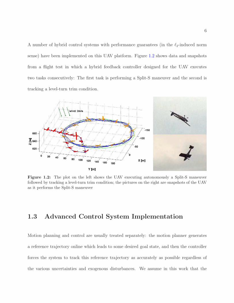
A number of hybrid control systems with performance guarantees (in the ℓ2-induced norm

sense) have been implemented on this UAV platform. Figure 1.2 shows data and snapshots

from a flight test in which a hybrid feedback controller designed for the UAV executes

two tasks consecutively: The first task is performing a Split-S maneuver and the second is

tracking a level-turn trim condition.

Figure 1.2: The plot on the left shows the UAV executing autonomously a Split-S maneuverfollowed by tracking a level-turn trim condition; the pictures on the right are snapshots of the UAVas it performs the Split-S maneuver

1.3 Advanced Control System Implementation

Motion planning and control are usually treated separately: the motion planner generates

a reference trajectory online which leads to some desired goal state, and then the controller

forces the system to track this reference trajectory as accurately as possible regardless of

the various uncertainties and exogenous disturbances. We assume in this work that the

7

planner carries out primitive-based motion planning [32, 33, 34]. Specifically, the motion

planner generates trajectories in real-time from a library of pre-specified motion primitives.

A motion primitive is a basic dynamically-feasible trajectory, namely a state history and

a corresponding control input that satisfy the nonlinear system equations over a finite or

a semi-infinite time interval. These primitives can be generated by solving optimization

problems involving the nonlinear system equations or by using flight simulators or actual

flight data.

In addition to the development and modeling of the UAV platform, this dissertation also

deals with the design and implementation of optimal controllers for the Telemaster UAV

along trajectories generated in real-time by appropriately concatenating library primitives.

We are mainly concerned with tracking dynamically feasible trajectories, that is, state and

control histories that satisfy the system equations of motion, as opposed to just following

geometric paths as in [35, 36], for instance. The motivation for this work is the control

of fixed-wing UAVs in cluttered dynamic environments, where operating in the presence of

moving obstacles necessitates that such complex dynamical systems with actuator limitations

traverse the planned trajectories rather accurately, hence the need for high-performance

controllers that can closely track dynamically feasible trajectories. In particular, we are

interested in applying linear matrix inequality (LMI) based control approaches that use the

ℓ2-induced norm as the performance measure and assessing the capability of these methods

in forcing a small fixed-wing UAV to closely track concatenated primitive trajectories under

relatively significant wind conditions. We consider LMI-based methods for ℓ2-induced norm

8

control of linear-time invariant (LTI) systems [37], linear time-varying (LTV) systems [38, 39],

and linear systems with uncertain initial conditions [20].

The first step in designing a model-based controller is to derive a reasonably accurate math-

ematical model of the physical system. The second step is to design a library of pre-specified

primitives, which provides the needed maneuverability. The library usually consists of trim

conditions and transitions between trim conditions. The trim conditions can be obtained

easily by solving for the equilibrium points of the nonlinear mathematical model. The tran-

sition maneuvers are not as easy to generate in general, but there are several methods that

can be utilized for this purpose. One method entails formulating the problem as a nonlinear

optimization problem and then using a software package such as GPOPS-II [40] to solve it.

Alternatively, the maneuvers can be obtained by recording pilot inputs and corresponding

system responses during an actual flight [41, 42]. Using this approach, aerobatic maneuvers

such as barrel roll and hammerhead can be generated. In this dissertation, we will use simple

feedback control to obtain transition maneuvers between trim conditions as well as recorded

pilot data to generate the Split-S maneuver.

There are two approaches typically used for the regulation of UAVs about trajectories. The

first and more common approach is to separate the control design problem into an inner

loop and an outer loop [43, 44, 45]. The outer loop determines the linear and angular rates

as well as the linear accelerations required to control the position and attitude. The inner

loop then computes the control surface deflections and throttle in order to track the rates

and accelerations commanded by the outer loop. In most cases, the inner loop is provided

9

by the onboard autopilot. A number of methods have been used to design the outer loop,

for instance, using control Lyapunov functions [43, 44] or receding horizon control [45]. The

second approach entails designing a single controller that directly controls the position and

attitude by prompting corrective control surface deflection and throttle commands [46, 47].

Some of the work in the literature that falls under this approach includes [46], in which

gain-scheduled H∞ controllers are used to track trim trajectories, and [47], where receding

horizon linear quadratic regulators are designed to track aerobatic maneuvers. One of the

advantages of using this approach is that stability is guaranteed for the closed-loop system.

The work herein uses the second approach.

When it comes to tracking trajectories generated in real-time from a library of prespec-

ified motion primitives, one way to go about solving the control synthesis problem is to

incorporate all possible connections between compatible library primitives into the control

design, as discussed in [34, 21]. Such an approach comes with stability and performance

guarantees across switching boundaries, but can become computationally prohibitive in the

case of large primitive libraries. In this dissertation, we address the control problem using

a decoupled approach, which is far less computationally intensive than the aforementioned

approach because in this case the controllers associated with the library primitives are de-

signed separately. We consider two concatenated primitive trajectories, which are assumed

to be generated online using a primitive-based motion planner and hence are not known

a priori. The first reference trajectory exhibits a “figure-8” geometric path and is formed

by concatenating seven primitives, which include three trim trajectories and four transition

10

maneuvers. The second trajectory is composed of a Split-S maneuver that settles into a

level-turn trim condition.

For the figure-8 trajectory, we design two discrete-time controllers and then analyze the

performance of these controllers in simulation and flight tests. The first controller is a

standard H∞ controller synthesized based on a discrete-time linear plant model. This plant

model is obtained by linearizing the nonlinear equations of motion of the UAV about a

straight and level trim condition and then discretizing the resulting model using zero-order

hold sampling. The second controller is a switching system, composed of three square ℓ2

induced norm sub-controllers synthesized based on linear discrete-time plant models with

uncertain initial conditions. These plant models are obtained by linearizing the nonlinear

system equations about the three trim trajectories: straight and level, steady right turn, and

steady left turn. We will refer to this controller as the switched uncertain initial condition

(UIC) controller. The uncertain initial conditions are introduced into the control design

to reflect the effects of switching between primitives. Based on the simulation and flight

testing results, we find that the performances of the two controllers are generally comparable;

however, the switched UIC controller achieves a superior performance when it comes to

tracking the reference altitude trajectory.

Based on these findings, we adopt the UIC control approach for tracking the second reference

trajectory. In this case, we design a standard finite horizon ℓ2-induced norm sub-controller,

with time-varying penalty weights on the state errors, for tracking the Split-S maneuver; it

was not necessary to take into account in the control design the uncertain initial state since

11

we made sure that the system state at the beginning of the experiment was as close to the

corresponding reference point as possible. In addition, a UIC sub-controller is designed to

track the subsequent level-turn trim trajectory. We demonstrate in simulation as well as

flight testing that the designed controller manages to closely track the reference trajectory

despite the modeling uncertainties, wind disturbances, and measurement noise.

In general, the switched systems of interest in this dissertation are composed of linear time-

invariant (LTI) and/or linear time-varying (LTV) subsystems obtained from linearizing the

nonlinear system equations describing the vehicle dynamics about a subset of the set of

prespecified primitives. As aforementioned, the switching between these subsystems and

ultimately their corresponding sub-controllers is dictated by the motion planning algorithm.

Related to this work is the paper [48] which provides a hybrid dynamics framework for the

design of guaranteed safe switching regions using reachable sets. The paper [49] also gives a

control algorithm for maneuver-based motion planning, which is robust to a certain class of

perturbations.

1.4 Contributions

The contributions of this dissertation are as follows:

1. We have developed a low-cost, open source, small UAV research platform, which is built

mostly of COTS components with a total price not exceeding $3000. The only non-

COTS components are the airdata probes, which are manufactured in-house following

12

a simple process and calibrated using the procedure from [16].

2. We have derived reasonably accurate models of the UAV, servos, and propulsion sys-

tem. The output error method is used to estimate both the longitudinal and lateral-

directional aerodynamic parameters from flight test data, which, to the author’s best

knowledge, is a first for small UAVs.

3. We have applied LMI-based control approaches that use ℓ2-induced norm as the per-

formance measure and assessed the capability of these methods in forcing a small

fixed-wing UAV to closely track concatenated primitive trajectories under relatively

significant wind conditions.

The work presented in this dissertation is based on the following two submitted journal

papers:

• Ony Arifianto and Mazen Farhood, “Development and Modeling of a Low-Cost Un-

manned Aerial Vehicle Research Platform,” submitted to Journal of Intelligent &

Robotic Systems.

• Ony Arifianto and Mazen Farhood, “Optimal Control of a Small Fixed-Wing UAV

about Concatenated Trajectories,” submitted to IEEE Transactions on Control Sys-

tems Technology.

Other published work that is related to the work presented herein appears in the following

conference paper:

13

• Ony Arifianto and Mazen Farhood, “Optimal Control of Fixed-Wing UAVs along Real-

Time Trajectories,” Proceedings of the ASME Dynamic Systems and Control Confer-

ence, 2012.

1.5 Organization

The outline of the dissertation is as follows. In Chapter 2, we present the autopilot system,

along with the ground control station, and discuss the development of the airdata probes. In

Chapter 3, we discuss the simple pendulum test method used to determine the moments of

inertia of the vehicle, and derive the mathematical models of the UAV, servos, and propulsion

system. Chapter 4 focuses on the design and validation of the control systems used for

tracking the figure-8 and the Split-S/level-turn trim trajectories. A brief summary is provided

in Chapter 5.

Chapter 2

Aerial Research Platform

Development

This chapter consists of two sections. The first describes all the components of the platform

avionics and the data flow among these components. The second section presents the de-

velopment process of two airdata probes, which are manufactured and calibrated in-house;

these sensors measure the airflow around the airplane and are used to determine the angle

of attack, sideslip, and airspeed of the UAV.

2.1 System Description and Architecture

In this section, we discuss the electronics used onboard the platform, which consist of actu-

ators, sensors, communication radios, and computers, as shown in Figure 1.1.

14

15

Actuators: The actuators are chosen based on the manufacturer’s (Hobby Express [17])

recommendations. Specifically, Futaba S3152 servos [50] are used for aileron, elevator, and

rudder control. A JETI ADVANCE 40 Pro (40 Amps programmable) electronic speed con-

troller (ESC) [51] is used to regulate the rotational speed of an AXI 2826/12 electric motor

[52], which is attached to a 13x8 APC propeller [53].

Sensors: The sensors used include a Microstrain 3DM GX3-25 Attitude and Heading Ref-

erence System (AHRS) (to measure attitude angles, angular rates, and linear accelerations)

[54], a Ublox LEA-4T Global Positioning System (GPS) receiver (to determine position)

[55], a VTI Technologies SCP1000 static pressure sensor (to determine altitude) [56], and

two airdata probes built in-house (for airflow measurements), which use two Freescale Semi-

conductor MPXV7002DP [57] differential pressure sensor arrays. Details on the development

of these probes are given in Section 2.2. The following are some useful comments on the use

of some of the aforementioned sensors:

- The accelerometers and rate gyros of the 3DM GX3-25 AHRS give measurements of linear

accelerations and angular rates about the aircraft’s body reference frame. An internal

Kalman filter algorithm uses these measurements, along with those of the AHRS magne-

tometers, to compute the Euler attitude angles. Adjustment of the Kalman filter weights

may be necessary when operating in areas with severe magnetic disturbances. In such

scenarios, it is advisable to place more confidence in the measurements given by the ac-

celerometers and rate gyros than those obtained from the magnetometers.

16

- The Ublox GPS receiver determines position in terms of latitude, longitude, and altitude.

Ground speed and course can be computed from this data, and will be utilized in the air-

data probe calibration process. In general, the precision of the altitude measurement from

this automotive grade GPS is insufficient for feedback control action when tracking rapid

maneuvers. To circumvent this issue, a measurement of the altitude based on pressure is

used instead. The pressure altitude is determined from the static pressure measurement

of the SCP1000 sensor using the standard atmospheric model [58]. To account for non-

standard day conditions, a bias is introduced so that the calculated pressure altitude on

the ground matches the corresponding altitude determined by the GPS.

- Since the avionics bay on the Telemaster has an opening directly behind the motor and

propeller, the pressure in the compartment is directly affected by the air mass exerted

by the propeller. To alleviate the resulting pressure build-up, several holes have been

drilled into the fuselage. To ensure that the SCP1000 sensor and the static ports of the

MPXV7002DP sensor array measure the static pressure in the fuselage, felt covers have

been installed on the inlet of the sensors.

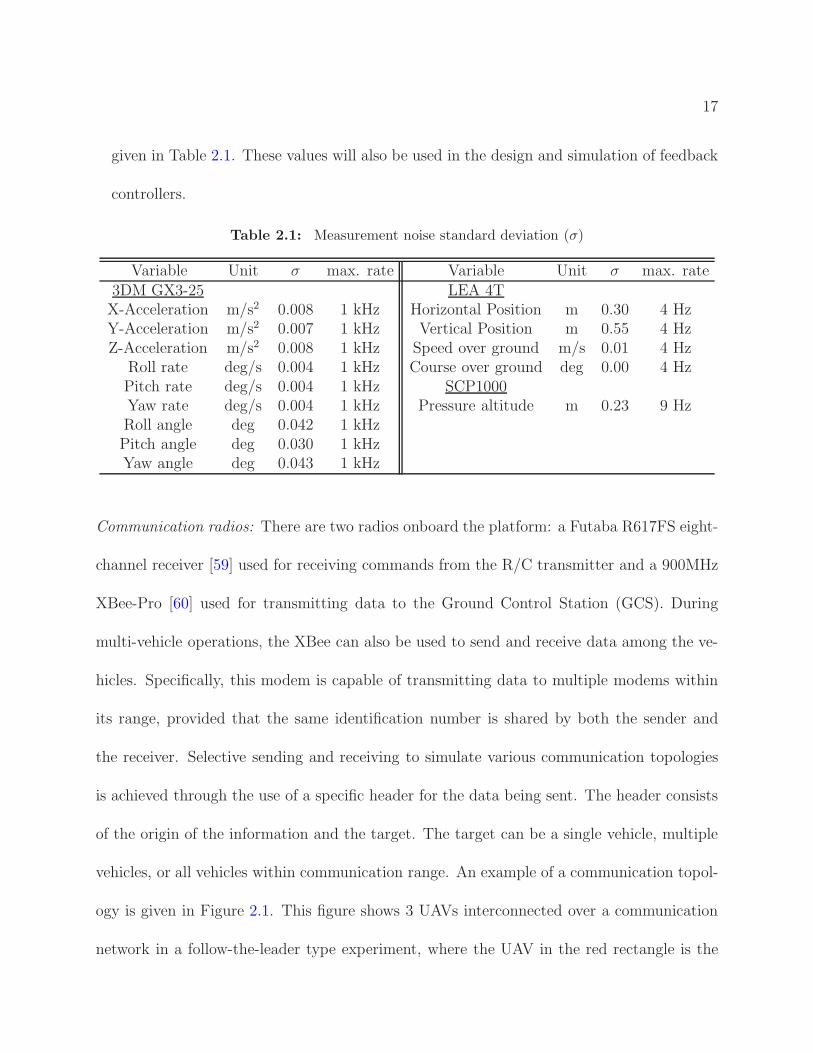
- The noise levels of the sensors, based on initial calibration and assessment, are given in

Table 2.1. The sensors are kept in a static condition, and measurements are recorded

for a period of time, specified based on the sampling rate to obtain sufficient data. The

standard deviation of the recorded data in this static condition is then used to describe

the measurement noise characteristics. It is assumed in this dissertation that sensor un-

certainties are only due to the presence of white noise, defined by the standard deviations

17

given in Table 2.1. These values will also be used in the design and simulation of feedback

controllers.

Table 2.1: Measurement noise standard deviation (σ)

Variable Unit σ max. rate Variable Unit σ max. rate3DM GX3-25 LEA 4TX-Acceleration m/s2 0.008 1 kHz Horizontal Position m 0.30 4 HzY-Acceleration m/s2 0.007 1 kHz Vertical Position m 0.55 4 HzZ-Acceleration m/s2 0.008 1 kHz Speed over ground m/s 0.01 4 Hz

Roll rate deg/s 0.004 1 kHz Course over ground deg 0.00 4 HzPitch rate deg/s 0.004 1 kHz SCP1000Yaw rate deg/s 0.004 1 kHz Pressure altitude m 0.23 9 HzRoll angle deg 0.042 1 kHzPitch angle deg 0.030 1 kHzYaw angle deg 0.043 1 kHz

Communication radios: There are two radios onboard the platform: a Futaba R617FS eight-

channel receiver [59] used for receiving commands from the R/C transmitter and a 900MHz

XBee-Pro [60] used for transmitting data to the Ground Control Station (GCS). During

multi-vehicle operations, the XBee can also be used to send and receive data among the ve-

hicles. Specifically, this modem is capable of transmitting data to multiple modems within

its range, provided that the same identification number is shared by both the sender and

the receiver. Selective sending and receiving to simulate various communication topologies

is achieved through the use of a specific header for the data being sent. The header consists

of the origin of the information and the target. The target can be a single vehicle, multiple

vehicles, or all vehicles within communication range. An example of a communication topol-

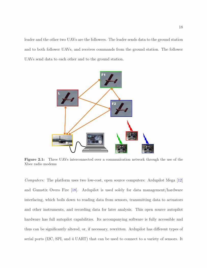
ogy is given in Figure 2.1. This figure shows 3 UAVs interconnected over a communication

network in a follow-the-leader type experiment, where the UAV in the red rectangle is the

18

leader and the other two UAVs are the followers. The leader sends data to the ground station

and to both follower UAVs, and receives commands from the ground station. The follower

UAVs send data to each other and to the ground station.

Figure 2.1: Three UAVs interconnected over a communication network through the use of theXbee radio modems

Computers: The platform uses two low-cost, open source computers: Ardupilot Mega [12]

and Gumstix Overo Fire [18]. Ardupilot is used solely for data management/hardware

interfacing, which boils down to reading data from sensors, transmitting data to actuators

and other instruments, and recording data for later analysis. This open source autopilot

hardware has full autopilot capabilities. Its accompanying software is fully accessible and

thus can be significantly altered, or, if necessary, rewritten. Ardupilot has different types of

serial ports (I2C, SPI, and 4 UART) that can be used to connect to a variety of sensors. It

19

has 16 analog-to-digital converters to handle sensors with analog voltage outputs as well as

8 pulse-width modulation (PWM) input channels and 8 PWM output channels that can be

used to drive servos. These features, along with the flexibility of the firmware, render the

board adaptable to a variety of sensor configurations.

All control computations are carried out by the Gumstix Overo Fire computer, which is a

single board computer powered by a 600MHz OMAP3530 microprocessor from Texas Instru-

ments [61]. The Overo runs a Linux Angstrom distribution as its operating system, and the

control algorithms are implemented in the Python programming language. This computer

is primarily selected for its small size. With length, width, and height dimensions of 58mm,

17mm, and 4.2mm, respectively, the Overo is advantageous for small UAV applications

where space and mass are major constraints. The Overo exchanges data with Ardupilot via

a serial port.

Before concluding this section, we will provide an overview of the data flow among the

computers, sensors, and servos onboard the airplane. Note that the engine electronic speed

controller (ESC) is considered as a servo in this scheme. A diagram of the data exchange

between these components is given in Figure 2.2. As the diagram shows, Ardupilot receives

data from the sensors and passes this data to the Overo computer. Overo then determines

the necessary control inputs based on this data and sends the calculated control commands

back to Ardupilot. Based on these commands, Ardupilot actuates the servos to drive the

control surfaces. Ardupilot also composes a data package, consisting of all the measurements

along with the control inputs to be sent to the onboard data logger as well as the ground

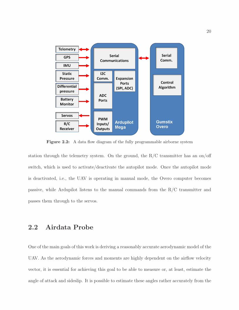
20

Figure 2.2: A data flow diagram of the fully programmable airborne system

station through the telemetry system. On the ground, the R/C transmitter has an on/off

switch, which is used to activate/deactivate the autopilot mode. Once the autopilot mode

is deactivated, i.e., the UAV is operating in manual mode, the Overo computer becomes

passive, while Ardupilot listens to the manual commands from the R/C transmitter and

passes them through to the servos.

2.2 Airdata Probe

One of the main goals of this work is deriving a reasonably accurate aerodynamic model of the

UAV. As the aerodynamic forces and moments are highly dependent on the airflow velocity

vector, it is essential for achieving this goal to be able to measure or, at least, estimate the

angle of attack and sideslip. It is possible to estimate these angles rather accurately from the

21

inertial velocity and attitude angles in the absence of significant winds, as demonstrated in

[62] and [63]. However, the condition of no significant winds is not easily met when dealing

with small UAVs flying at low speeds. Thus, developing sensors that can measure the angle

of attack and sideslip is instrumental for obtaining an adequate aerodynamic model of a

small UAV.

2.2.1 Probe design and manufacturing

Common methods for measuring the airflow direction use mechanical vanes, differential

pressure tubes, or null-seeking pressure tubes, as outlined in [64]. Due to potential design

and implementation difficulties, the use of mechanical vanes and null-seeking pressure tubes

is not preferable in the case of small UAVs where size and weight are major constraints. To

the best of our knowledge, null-seeking pressure tubes have never been used on small UAVs.

Mechanical vanes, on the other hand, have been used successfully on a small UAV in [6] to

measure the airflow direction.

There are various differential probe designs that can be used to measure the airflow vector.

These designs vary in the shape of the probe tip and/or the number of pressure holes. A

comparison of measurement results using different designs of differential probes is given in

[14]. As stated in [65], the accuracy of the differential probe measurements is proportional

to the number of pressure holes, and hence comes at the expense of increased manufacturing

complexity. The shape of the tip also affects the accuracy of the probe measurements. For

22

instance, an airdata probe with a perfectly spherical tip shape gives accurate measurements

without the need for calibration because there are mathematical formulas available in the

literature that can be used to directly compute the airspeed, angle of attack, and sideslip from

the pressure differences in this case. Manufacturing such a probe, however, is challenging.

In our case, we have opted to design a five-hole probe with a conical tip shape for the

following reasons: (1) There are many publications on the calibration and testing of five-

hole probes; and (2) it is possible to manufacture this probe from commercially available

materials using conventional machining techniques. We have built and calibrated two probes,

each mounted on a wing of the airplane at a distance of 16 inches from the plane of symmetry

with the port holes situated about 6 inches from the wing leading edge; see Figure 1.1. This

configuration maintains lateral balance and ensures that the effects of the propeller wash and

wing interference on the airflow measurements are insignificant. Both probes are comparable

in quality and are used together in our platform for redundancy. In the following, we will

just focus on one probe.

The CAD model of the five-hole probe that we have designed is given in Figure 2.3, along

with the final product. The figure shows the holes arrangement at the tip of the probe. The

probe consists of five small aluminum tubes, glued together using JB Weld plastic steel to

form the desired plus-sign configuration, and then encased in a larger aluminum tube. The

tubes used are sold in most hardware stores. The length of the probe is 203.2mm, and the

tip diameter is 5.56mm. Each of the five small tubes has an outer diameter of 1.60mm and

an inner diameter (hole diameter) of 0.89mm. Then, the ratio of the hole diameter to the

23

Figure 2.3: Five-hole probe and its CAD drawing

tip diameter is 0.16. Although this ratio is relatively small compared to the one in [14], the

number is fairly close to newer designs, such as those in [66] and [67].

The tip design is conical with 90 angle. As observed in [14, 15], this tip design yields

reasonably accurate measurements of the angle of attack and sideslip at low speeds and

can be calibrated to measure these angles within the range ±22.5. For such a tip design,

there are no mathematical formulas that directly relate the pressure differences to the angle of

attack and sideslip, as in the case of the perfectly spherical tip shape. Hence, the relationship

between the measured pressure at each hole (port) and the airflow velocity vector can only

be determined by experiment. The experiment, along with the required data processing and

24

Figure 2.4: Five-hole probe calibration process

curve fitting, is henceforth referred to as probe calibration.

2.2.2 Probe calibration

The calibration of the probe was performed in the Subsonic Open Jet Wind Tunnel at

Virginia Tech following the procedure given in [16]. Figure 2.4 shows the experiment setup.

In this setup, the probe is placed in the middle of the test section of the wind tunnel on a

turntable that can be rotated to vary the sideslip angle. The angle of attack can also be varied

by rotating the rod on which the turntable is mounted. During calibration, the rotational

speed of the wind tunnel fan is increased from 0 to 1180 rpm (maximum achievable speed)

25

in increments of 200. The airflow velocity (in m/s) is about 0.021 times the fan rotational

speed (in rpm). Hence, at a fan speed of 1180 rpm, the resultant airflow velocity is about

24.78m/s. For each considered rotational speed, the angle of attack and sideslip are varied

from −20 to +20 in 5 increments, with the pressure at all ports of the probe measured

in each configuration. The pressure measurements for various values of the angle of attack

and sideslip at a fan speed of 400 rpm are shown in Figure 2.5.

−20 −10 0 10 20−20

−10

0

10

20

β [deg]

α [d

eg]

P1 [in H2O] at 400 rpm

375.98

376

376.02

376.04

376.06

376.08

376.1

−20 −10 0 10 20−20

−10

0

10

20

β [deg]

α [d

eg]

P4 [in H2O] at 400 rpm

376

376.05

376.1

−20 −10 0 10 20−20

−10

0

10

20

β [deg]

α [d

eg]

P5 [in H2O] at 400 rpm

376.09

376.1

376.11

376.12

376.13

376.14

−20 −10 0 10 20−20

−10

0

10

20

β [deg]

α [d

eg]

P2 [in H2O] at 400 rpm

376

376.05

376.1

−20 −10 0 10 20−20

−10

0

10

20

β [deg]

α [d

eg]

P3 [in H2O] at 400 rpm

376.02

376.04

376.06

376.08

376.1

376.12

Figure 2.5: Pressure distribution at various values of the angle of attack (α) and sideslip (β) forall ports of the probe

As mentioned earlier, during calibration process, the pressures at all ports of the probe, i.e.,

p1, p2, . . . , p5, are measured for each configuration, where pi is the pressure at port i and

26

the port numbering is shown in Figure 2.3. As given in [16], it is possible to approximately

compute the angle of attack, α, and sideslip, β, from the pressures p1, . . . , p5 as follows:

α =a0 + a1Cpα + a2Cpβ + a3C

2pβ

+ a4C3pβ

1 + a5Cpα + a6Cpβ + a7C2pβ

+ a8C3pβ

, (2.1)

β =b0 + b1Cpα + b2Cpβ + b3C

2pα

+ b4C2pβ

+ b5CpαCpβ

1 + b6Cpα + b7Cpβ + b8C2pα

+ b9C2pβ

+ b10CpαCpβ, (2.2)

where pav = 0.25(p1 + p2 + p3 + p4), Cpα =p3 − p1p5 − pav

, and Cpβ =p4 − p2p5 − pav

.

Given the data collected in the calibration process, the calibration coefficients a0, a1, . . . , a8

and b0, b1, . . . , b10 in equations (2.1–2.2) are obtained by solving a least-squares problem by

linear regression. The fitting surface and goodness of fit for the angle of attack and sideslip

are shown in Figure 2.6 and 2.7. The coefficient of determination, or R2, value for the angle

of attack data fitting is 0.9949 and that for the sideslip data fitting is 0.9972.

The airspeed Va can be computed from the static pressure ps and total pressure pt, namely,

Va =

√

2(pt − ps)

ρ,

where ρ denotes the air density. While it is possible to measure ps and pt during calibration by

using a pitot-static tube aligned with the direction of the airflow, it is impractical to replicate

this setup on the actual UAV. Alternatively, as suggested in [16], we can approximately obtain

the values of the static and total pressures, and hence the airspeed, from the angle of attack

27

−50

5−5

05

−50

0

50

Cpp [−]

α Data Fitting R2=0.9949

Cpt [−]

α [d

eg]

Figure 2.6: Angle of attack surface fitting

and sideslip, along with the pressures p1, . . . , p5, as follows:

ps =Cp5pav − Cpavp5Cp5 − Cpav

and pt = ps +p5 − psCp5

,where

Cp5 =c0 + c1β + c2β

2 + c3β3 + c4α + c5α

2

1 + c6β + c7α + c8α2 + c9α3, and (2.3)

Cpav = d0 + d1β + d2α+ d3β2 + d4α

2 + d5αβ + d6β3 + d7α

3 + d8βα2 + d9β

2α. (2.4)

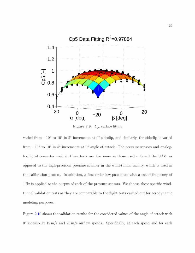
The coefficients c0, c1, . . . , c9 and d0, d1, . . . , d9 in equations (2.3–2.4) are also obtained by

solving a least-squares problem by linear regression. As shown in Figure 2.8 and 2.9, the

R2 value for the Cp5 data fitting is 0.9788 and that for the Cpav data fitting is 0.9676.

Our calibration results, and specifically the R2 values, are comparable to those obtained

28

−50

5 −50

5

−50

0

50

Cpp [−]

β Data Fitting R2=0.99721

Cpt [−]

β [d

eg]

Figure 2.7: Angle of sideslip surface fitting

in [16]. This observation is noteworthy considering that the authors in [16] utilize a more

sophisticated manufacturing process in building their probe, in addition to a closed-circuit

wind tunnel for calibration, which generally generates less turbulent airflow compared to an

open-jet tunnel.

2.2.3 Validation and analysis

The calibration results are validated by wind-tunnel testing as well as flight testing. In the

wind-tunnel tests, the probe is evaluated at a low airflow speed of about 12m/s and a high

airflow speed of about 20m/s; these speeds correspond to the lower and upper limits of

typical operation of the UAV platform, respectively. For each speed, the angle of attack is

29

−20 0 20−200200.4

0.6

0.8

1

1.2

1.4

β [deg]

Cp5 Data Fitting R2=0.97884

α [deg]

Cp5

[−]

Figure 2.8: Cp5 surface fitting

varied from −10 to 10 in 5 increments at 0 sideslip, and similarly, the sideslip is varied

from −10 to 10 in 5 increments at 0 angle of attack. The pressure sensors and analog-

to-digital converter used in these tests are the same as those used onboard the UAV, as

opposed to the high-precision pressure scanner in the wind-tunnel facility, which is used in

the calibration process. In addition, a first-order low-pass filter with a cutoff frequency of

1Hz is applied to the output of each of the pressure sensors. We choose these specific wind-

tunnel validation tests as they are comparable to the flight tests carried out for aerodynamic

modeling purposes.

Figure 2.10 shows the validation results for the considered values of the angle of attack with

0 sideslip at 12m/s and 20m/s airflow speeds. Specifically, at each speed and for each

30

−20 0 20−20020

0.2

0.3

0.4

0.5

0.6

β [deg]

Cpav Data Fitting R2=0.96763

α [deg]

Cpa

v [−

]

Figure 2.9: Cpav surface fitting

Figure 2.10: Angle of attack validation at 12m/s airflow speed (left) and 20m/s speed (right)

value of the angle of attack, the test is run for 30 seconds, and samples are collected at

20Hz, i.e., we end up with 600 samples in total for each test. Thus, the total number of

samples for all the angle of attack tests at each speed is 3000. The measurement error is

31

defined as the difference between the measured value and true value of the angle of attack.

We then have 3000 samples of the measurement error at 12m/s airflow speed (low speed)

and another 3000 samples at 20m/s (high speed). Note that the measurement discrepancies

are due to calibration errors as well as instrumentation errors (because of the use of the

actual, less accurate sensors). The following analysis of the aforementioned two sets of data

is based on [68]. Given these data, we find that the angle of attack can be measured with

an accuracy of 0.67 at low speed and 0.46 at high speed, where the accuracy is given in

terms of the root-mean-square (RMS) of the measurement error. The RMS is defined as

RMS =√

1N

∑N

i=1 e2i , where N is the number of samples, which is 3000 for each speed, and

ei is the ith sample of the measurement error. The RMS measure is used because the mean

of the error is not zero; specifically, there is a measurement bias of 0.27 at low speed and

−0.06 at high speed. Assuming the error is normally distributed about the nonzero mean

value, then, for each speed, the number of samples that lie within the range ±RMS is equal

to 12

(

ERF(

RMS−µσ√2

)

+ ERF(

RMS+µ

σ√2

))

, where σ is the standard deviation of the error, µ is

the mean value, and ERF(η) is the error function defined as ERF(η) = 1√2

∫ η

−η e−ξ2dξ. Hence,

80.6% of the measurement error samples lie within ±0.67 at low speed and 83.9% lie in the

range ±0.46 at high speed. Additionally, 95% of the error samples lie in the range ±0.99

at low speed and ±0.64 at high speed.

Figure 2.11 shows the validation results for the considered values of the sideslip with 0 angle

of attack at 12m/s and 20m/s speeds. The samples of the measurement error are collected

in the same way as in the angle of attack case. The measurement error in this case also tends

32

Figure 2.11: Angle of sideslip validation at 12m/s airflow speed (left) and 20m/s speed (right)

to decrease as the airflow speed increases. The RMS is 0.92 at low speed and 0.54 at high

speed. 67.9% of the samples lie within ±0.92 at low speed and 81.9% lie within ±0.54 at

high speed. The 95% confidence intervals are [−1.37, 1.37] at low speed and [−0.79, 0.79]

at high speed.

The probe is next tested in flight. The test entails maintaining the airplane in straight

(and preferably level) flight, as sensor measurements, including those from the probe, are

recorded. In this scenario, as long as the wind disturbances are relatively insignificant, the

angle of attack should be approximately equal to the pitch angle minus the flight path angle.

In our tests, we managed to maintain the airplane in almost level flight (i.e., at a roughly

zero flight path angle). Figure 2.12 shows that the measured values of the angle of attack

obtained from the probe correlate well with the measurements of the pitch angle from the

AHRS sensor. Note that the 4 bias between the measurements from the probe and those

from the AHRS is due to the fact that the probe is installed on the wing, which has an angle

of incidence of approximately 4. Note that this type of test is not suitable for the validation

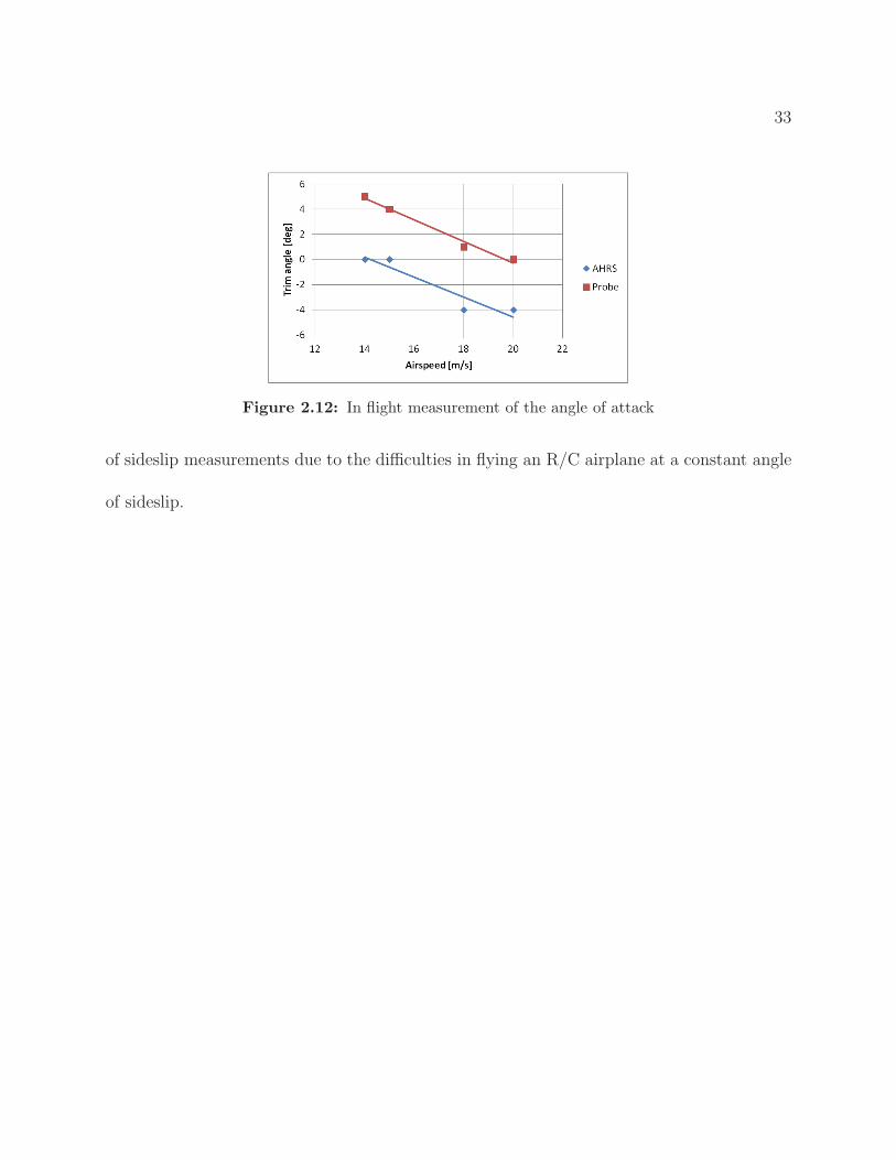
33

Figure 2.12: In flight measurement of the angle of attack

of sideslip measurements due to the difficulties in flying an R/C airplane at a constant angle

of sideslip.

Chapter 3

Mathematical Model Development

In order to design dynamically feasible trajectories offline and develop high-performance

feedback controllers, a reasonably accurate model of the aircraft dynamics is required. A

combination of semi-empirical, frequency domain, and time-domain identification techniques

are utilized to obtain a mathematical representation of each major component of the system.

This chapter is divided into five sections: the first gives the equations of motion of the UAV;

the second presents the test method used to determine the moments of inertia; the third

describes the experiment conducted to obtain the frequency response of each actuator; the

fourth focuses on the propeller thrust modeling; and the last section presents the parameter

estimation process used for deriving the aerodynamic model of the UAV.

34

35

3.1 Aircraft Equations of Motion

The dynamics of the UAV are described by standard rigid-body six-degree-of-freedom equa-

tions of motion in the aircraft body reference frame. Before giving these equations, we define

the following reference frames:

I := inertial reference frame with X-axis pointing North, Y-axis pointing East, and

Z-axis pointing down (NED)

B := body reference frame, fixed to the center of gravity of the UAV, with X-axis

pointing to nose, Y-axispointing to starboard wing, and Z-axis pointing down

The following notations are introduced to concisely present the equations of motion, as

suggested by [69, 46, 70]:

P = position of the center of gravity in I = [N, E, −H ]T

V = linear velocity of the center of gravity relative to I, expressed in B

= [u, v, w]T

Vw = linear velocity of the wind relative to I, expressed in B = [uw, vw, ww]T

V = linear velocity of the center of gravity relative to wind, expressed in B

= [u− uw, v − vw, w − ww]T

Va = airspeed of the UAV =√

(u− uw)2 + (v − vw)2 + (w − ww)2

36

Ω = angular velocity of B relative to I, expressed in B = [p, q, r]T

Λ = vector of Euler angles with respect to I = [φ, θ, ψ]T

IBR = rotation matrix from B to I in SO(3), given in terms of Λ

G = gravitational vector = g[− sin θ, cos θ sinφ, cos θ cos φ]T ,

where g is the gravitational constant

We assume that the earth is flat and the gravity field is constant (g = 9.80665m/s2). Let

δ = [δe, δa, δr, δt]T , where δe, δa, and δr denote the elevator, aileron, and rudder deflections,

respectively, and δt designates the throttle input. Note that the aforementioned control

surface deflections are the actual deflections, that is, the outputs of the servomotors used to

deflect the control surfaces on the UAV. The commanded deflections, which are the inputs

to the servomotors, are denoted by δce, δca, and δ

cr. The three servomotors used onboard the

UAV are identical and each is modeled as a second-order system obtained by measuring the

frequency response, as discussed in Section 3.3. We can then express the equations of motion

as follows:

V = m−1F (V ,Ω, δ) +G− Ω× V (3.1)

Ω = J−1M(V ,Ω, δ)− J−1(Ω× JΩ) (3.2)

P = IBR(Λ)V (3.3)

Λ = E(φ, θ)Ω (3.4)

where m = 3.24 kg is the mass of the airplane, J is the moment of inertia tensor, F (V ,Ω, δ)

37

denotes the aerodynamic and propulsion forces, M(V ,Ω, δ) denotes the aerodynamic and

propulsion moments, and

E(φ, θ) =

1 sin φ tan θ cosφ tan θ

0 cosφ − sinφ

0 sinφ/ cos θ cosφ/ cos θ

.

The ground testing procedures used to obtain the moments of inertia of the airplane, and

hence the inertia tensor J , are described in Subsection 3.2. Subsections 3.4 and 3.5 give the

aerodynamic and propulsion models. Note that we assume the propeller does not signifi-

cantly affect the airflow over the airplane. Consequently, we approach the aerodynamic and

propulsion modeling separately. We can then write F and M as

F (V ,Ω, δ) = FA(V ,Ω, δe, δa, δr) + FP (V , δt),

M(V ,Ω, δ) =MA(V ,Ω, δe, δa, δr) +MP (V , δt),

(3.5)

where (·)A and (·)P denote the aerodynamic and propulsion components, respectively.

3.2 Moments of Inertia

The moments of inertia of a full-scale aircraft about the roll and pitch axes are typically

determined using the compound pendulum method, whereas the moment of inertia about

the yaw axis is obtained using the bifilar pendulum approach, as described in [25, 26, 27]. In

38

the case of a small UAV, the vehicle can be be easily tilted sideways, and so the moment of

inertia about the yaw axis can also be determined using the compound pendulum method.

That way, the same setup can be used to perform all the experiments. The bifilar pendulum

method can also be used to determine all the moments of inertia of a small UAV, as shown,

for example, in [71], provided that the testing setup is appropriately configured to avoid

the inadvertent excitation of the swaying mode, which could otherwise result in significant

measurement errors as discussed in [72]. Thus, either of the aforementioned test methods

can be used to compute the moments of inertia of a small UAV. In our case, we have used

the compound pendulum method simply for convenience.

The moments of inertia about the roll, pitch, and yaw axes are determined in three separate

experiments. In each experiment, the UAV is positioned appropriately on a wire suspended

cradle, as shown in Figure 3.1, in order to obtain the moment of inertia about the desired axis.

The experiment entails finding the oscillation period of the pendulum and then computing

from this period the moment of inertia by applying a simple mathematical formula. It

is indicated in [26] and observed in our preliminary tests that the compound pendulum

method is sensitive to the length of the suspending wires. Specifically, the accuracy of the

measurements obtained using this method degrades as the distance from the pivot axis of

the pendulum to the center of gravity of the UAV, denoted by L, increases. This finding

can also be verified by examining the mathematical formula used to compute the moment

of inertia and doing some sensitivity analysis. The formula for computing the moment of

inertia, I, is based on the linearized equation of motion of the compound pendulum and

39

Figure 3.1: Moments of inertia testing setup: wire suspended cradle (left); setup to determinethe moment of inertia about the pitch axis (top middle), the roll axis (bottom middle), and theyaw axis (right)

is given by I =mgLT 2

4π2− mL2, where T is the oscillation period of the pendulum, g is

the acceleration due to gravity, and L is as defined before. As the major source of error

in computing the moment of inertia is the inaccuracy in the measurement of the oscillation

period, it is important to examine the local sensitivity of I with respect to T . Suppose

that the true value of the moment of inertia is In, and the corresponding oscillation period

is Tn. Then, the local sensitivity of I with respect to T is∂I

∂T=

1

π

√

mgL (In +mL2).

It is clear from the preceding equation that, as L increases, any small discrepancy in the

period measurement would yield a more significant error in the computation of the moment

of inertia.

As mentioned before, the test setup for determining the moments of inertia is shown in

Figure 3.1. The cradle that holds the vehicle is connected to the pivot points on the ceiling

40

by four braided steel wires. The cradle consists of a wooden frame, along with four eyescrews

to attach the frame to the steel wires. The cradle is located at 1.18m from the pivot axis

and has a mass of 1.27 kg. When placing the vehicle on the cradle, it is important to make

sure that the center of gravity of the vehicle is as close as possible to the center of the cradle.

The test setup does not require any specific mounting apparatus, and therefore can be used

for multiple airplane models of similar size. Prior to the testing of the UAV, a calibration

test is performed to determine the moment of inertia of the cradle, following the standard

compound pendulum procedure. The moment of inertia of the cradle about the pivot axis

is found to be 1.96 kgm2. Three experiments are then performed to determine the moments

of inertia of the UAV about the roll, pitch, and yaw axes (X, Y, and Z axes in the body

reference frame), which are denoted by Ixx, Iyy, and Izz, respectively. The location of the

center of gravity of the UAV in each of these experiments slightly changes based on the

orientation of the airplane with respect to the cradle. These locations, measured from the

pivot axis of the pendulum, are 1.22, 1.35, and 1.21 m corresponding to the configurations

used to determine Ixx, Iyy, and Izz, respectively. The mass of the UAV is 3.24 kg and is

slightly increased to 3.31 kg when determining Ixx due to the addition of a wooden bar to

hold the airplane in place during this test.

To determine the moment of inertia about a specific axis of the UAV, 3 tests are performed.

In each of these tests, the time required to complete 50 oscillations is recorded. Then, the

average of the three recorded values, denoted by T50, is used to compute the moment of

inertia by applying the following equation:

41

Table 3.1: Moments of inertia of the Telemaster UAV

Ixx Iyy IzzT50 114.89 118.25 115.36 sωn 2.73 2.66 2.72 rad/sI 0.21 0.31 0.48 kgm2

I2 =g(m1L1 +m2L2)

ω2n

− I1 −m2 L22,

where ωn = 100π/T50 is the frequency of oscillation, m1 is the mass of the cradle, m2 is the

mass of the UAV, L1 is the location of the center of gravity of the cradle, L2 is the location

of the center of gravity of the UAV (both locations measured from the pivot axis), I1 is the

moment of inertia of the cradle about the pivot axis, and I2 is the moment of inertia of the

UAV about its body axis. Table 3.1 gives the calculated values of the moments of the inertia

of the UAV. Concerning the computation of the inertia tensor J , it is reasonable to assume

in our case that the “cross-product-of-inertia” terms, Ixy, Ixz, and Iyz, are all zeros, and

hence, we have

J =

Ixx −Ixy −Ixz

−Ixy Iyy −Iyz

−Ixz −Iyz Izz

=

0.21 0 0

0 0.31 0

0 0 0.48

.

3.3 Servo Model

Three servomotors are used to deflect the control surfaces on the airplane. These servos

are identical and their dynamics are described by the same second-order system model. For

42

instance, the system equations of the servo used to deflect the elevator are:

x1s

x2s

δe

=

0 1 0

−ω2ns −2ζsωns ω2

ns

1 0 0

x1s

x2s

δce

, (3.6)

where x1s and x2s are the internal states of the servo, δce is the commanded elevator deflection,

δe is the actual deflection, ωns is the natural frequency of the servo mechanism, and ζs is the

damping ratio.

This model, and specifically the natural frequency and damping ratio of the servo, are ob-

tained experimentally by measuring the frequency response. The frequency response test is

performed by sending continuous sinusoidal command inputs at different frequencies to the

servo, one at a time, and, in each case, recording the commanded signal and the correspond-

ing response simultaneously. The frequencies are chosen to cover a wide range about the

cutoff frequency of the servo. The test setup is given in Figure 3.2.

To measure the servo response, a potentiometer is mounted such that the shaft of the poten-

tiometer is aligned with that of the servo. This potentiometer is supplied with 5V voltage by

an Ardupilot board and produces 0− 5V output based on the angular position of its shaft.

The Ardupilot is also used to generate the reference command and send it to the servo, as

well as record the output from the potentiometer. The potentiometer readings for a number

of commanded servo positions are recorded prior to the frequency response test in order to

determine the calibration curve for this sensor. At each test frequency, the magnitude and

43

Figure 3.2: Test setup for the frequency domain identification of the Futaba S3152 servo model

phase shift of the frequency response are determined by comparing the commanded input

sinusoid and the measured steady-state output signal; the values obtained are given in Table

3.2.

Table 3.2: Futaba S3152 frequency response

Frequency Magnitude PhaseHz - rad0.01 1.00 0.000.10 1.00 -0.041.00 0.96 -0.572.00 0.81 -1.514.00 0.31 -3.025.00 0.19 -3.14

Frequency domain fitting is applied to the test data, with the natural frequency and damping

44

10−2

10−1

100

101

102

0

0.5

1

1.5

Frequency [rad/s]

Mag

nitu

de [−

]

ωns

= 13.7 ; ζs = 0.67

10−2

10−1

100

101

102

−4

−2

0

Frequency [rad/s]

Pha

se [r

ad]

fitdata

Figure 3.3: Curve fitting of the servo test data

ratio used as the fitting parameters. Since the system is fairly simple, the natural frequency

and damping ratio are adjusted manually to obtain a satisfactory fit. A natural frequency of

ωns = 13.7 rad/s and a damping ratio of ζs = 0.67 are obtained for the Futaba S3152 servo

used in this work. The test data in Table 3.2 and the second-order system fit are shown in

Figure 3.3.

3.4 Propulsion Model

The propulsion system of the Telemaster UAV consists of a 760 RPM/Volt electric motor

and a 13 × 8 inch propeller. The engine is powered by a 3S LiPo battery and controlled by

45

Figure 3.4: Relationship between the throttle command δt, which is a PWM signal, and theengine RPM

a 40 Amps speed controller. We now derive a propulsion model of our system. We assume

the propeller axis to be perfectly aligned with the body X-axis. As a result, the propeller

thrust will be applied along the body X-axis only, that is, FP (V , δt) = [T (Va, δt), 0, 0]T , and

further, the thrust will not generate any moments, namely MP (V , δt) = 0. The propulsion

system model maps the throttle command δt, which is a PWM (pulse-width modulation)

signal, to the generated propeller thrust T (Va, δt), given a certain airspeed. We assume that

the dynamics of the propulsion system are fast enough that we may ignore the transient

behavior. We also assume that, even under nonzero airspeed conditions, the electronic speed

controller (ESC) is able to ensure that, for a constant throttle command, the engine runs at

a constant RPM.

46

Figure 3.5: Thrust prediction as a function of airspeed and engine RPM (Javaprop)

We have obtained experimentally a look-up table, represented graphically in Figure 3.4,

that can be used to map a throttle command into the corresponding engine RPM through

interpolation. Then, given the engine RPM and the current airspeed, we can compute the

generated propeller thrust using look-up tables obtained from the propeller analysis applet,

Javaprop [24]. This applet uses blade element theory to return a thrust profile based on the

propeller geometry. The complete thrust model, which relates the engine RPM and airspeed

to propeller thrust, is given in Figure 3.5. Notice that, for a propeller rotating at a constant

RPM, increasing the airspeed decreases the effective angle of attack of the propeller blade

and, as a result, decreases the propeller thrust. Increasing the airspeed beyond a certain

value will reverse the effective angle of attack, and hence cause the propeller to generate drag

47

Figure 3.6: Test setup for measuring propeller thrust at zero airspeed

instead of thrust. From this figure, we also observe that the maximum thrust-to-weight ratio

of the Telemaster is about 0.41, which is a typical value for a trainer class R/C airplane.

The thrust predictions generated by Javaprop at zero airspeed (static data) are verified

through ground testing. The test setup is given in Figure 3.6, which shows the engine

mounted on an apparatus that is attached to a weight scale, with the propulsion system set

up in a pusher configuration, that is, the generated thrust pushes the whole test apparatus

downward. We use the weight scale and a tachometer to obtain the values of the propeller

thrust and engine RPM, respectively, for each considered throttle setting. The static thrust

data returned by Javaprop and those obtained from two ground tests, performed using two

different batteries, are given in Figure 3.7. The figure clearly shows that the Javaprop

48

Figure 3.7: Static thrust data along with Javaprop predictions

predictions closely match the static test data.

3.5 Aerodynamic Model

The goal of aerodynamic modeling is to obtain a reasonably accurate mapping from the

airplane state and control variables to the aerodynamic forces and moments in the operating

envelope. Thus, we need to find formulas for FA(V ,Ω, δe, δa, δr) = [FX , FY , FZ ]T and

MA(V ,Ω, δe, δa, δr) = [MX , MY , MZ ]T , as defined in (3.5), where Fi is the component of the

aerodynamic force in the body i-axis and Mi is the aerodynamic moment about the body

i-axis. Specifically, we aim to determine the force coefficients Ci = Fi/(QS), for i = X, Y, Z,

49

and the moment coefficients Cl = MX/(QS b), Cm = MY /(QS c), and Cn = MZ/(QS b),

where Q = 0.5 ρ V 2a is the dynamic pressure, with ρ being the air density, S is the wing area,

b is the wing span, and c is the mean aerodynamic chord. The values of the aforementioned

geometrical parameters can be found in Table 1.1.

The aerodynamic model can be obtained using several methods, including those based on

semi-empirical techniques, computational fluid dynamics (CFD), wind tunnel testing, and

flight testing. A semi-empirical method typically uses basic aerodynamic theories, along

with some experimental data, to generate an aerodynamic model based on some geometrical

parameters of the airplane. There are available software, such as digital DATCOM [73],

which use semi-empirical methods to predict the aerodynamic characteristics of airplane.

DATCOM, in particular, takes some geometrical parameters as inputs and outputs aero-

dynamic coefficients and stability derivatives. Applying such methods to find aerodynamic

models for small UAVs may be unfavorable in general because most of the experimental data

used by these methods are obtained for full-scale aircraft. There are several, freely available,

linear CFD codes based on vortex lattice analysis, such as Athena Vortex Lattice [74] and

Tornado [75], that can be used to develop aerodynamic models for small UAVs. The CFD

approach generally gives a satisfactory aerodynamic model in the linear region of the aero-

dynamic force and moment curves. However, this approach does not take into account the

effects of gaps between the control surfaces and the wings or tails in computing the forces

and moments generated by the control surface deflections. The drag prediction is also opti-

mistic in this case, that is, the resulting model underestimates the value of drag; the reason

50

is the CFD method only considers the drag generated by the pressure distribution around

the wings and fuselage and neglects the drag due to skin friction and appendices such as

the landing gear. Wind tunnel testing offers accurate and comprehensive aerodynamic data

to develop a high-fidelity model, but this comes at the expense of high cost and relatively

long model development time [76]. In the case of small, low-cost UAVs, the cost and time

to perform the necessary wind tunnel tests can be prohibitive. System identification and/or

parameter estimation techniques can be used to develop aerodynamic models from flight test

data [28, 77, 78]. The structure of the aerodynamic model may be determined based on the

test data by using, for instance, a stepwise regression method (system identification), or it

can be simply postulated. Parameter estimation techniques can then be used to estimate

the values of the aerodynamic coefficients.

In this dissertation, the aerodynamic model is obtained from flight test data using the output

error method for parameter estimation in the time domain. The output error method is

a maximum likelihood estimator for data with measurement noise [79]. This method is

asymptotically unbiased and consistent, that is, the estimated parameters will approach their

true values as the number of measurements increases [77]. It is computationally manageable,

especially when compared to the more sophisticated filter error method. But, unlike the filter

error method, the output error approach is not well-suited to handling process noise, and

so it is important to carry out the flight tests in the absence of significant atmospheric

disturbances. Details on the use of the output error method for aerodynamic parameter

estimation can be found in [28, 77]. The structure of the aerodynamic model used is given

51

in Eq. (3.7), as suggested in [80]. This structure is chosen so that a single model can be used

to capture the UAV dynamics in the entire operating envelope of interest.

CX = CX0+ CXαα + CX

α2α2

CY = CY0 + CYββ + CYpp b

2Va+ CYr

r b

2Va+ CYδaδa + CYδrδr

CZ = CZ0 + CZαα + CZδeδe + CZα2α2 (3.7)

Cl = Cl0 + Clββ + Clpp b

2Va+ Clr

r b

2Va+ Clδaδa + Clδrδr

Cm = Cm0+ Cmαα+ Cmq

q c

2Va+ Cmδeδe + Cm

α2α2

Cn = Cn0 + Cnββ + Cnpp b

2Va+ Cnr

r b

2Va+ Cnδaδa + Cnδrδr

The flight tests for parameter estimation in our case are performed by a pilot on the ground

controlling the airplane remotely. Hence, only a few standard maneuvers for parameter

estimation can be successfully performed. These maneuvers capture the dutch-roll, bank-

to-bank, and short period motions of the aircraft. Specifically, we employ standard control

input patterns for time-domain parameter estimation [28] to excite the vehicle. The input

patterns used are different for each control actuator: doublet inputs are used for the rudder

to capture the dutch-roll mode, 1-2-1 for the aileron to capture the bank-to-bank motion,

and 3-2-1-1 for the elevator to capture the short period mode. These integers indicate the

number of time steps to hold a control actuator at a specified position before moving it to

the same position in the opposite direction. Figure 3.8 illustrates the shape of each control

surface input to be executed during the flight tests. In this figure, the time step ∆t and the

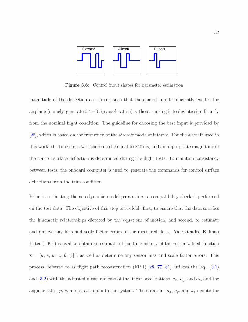
52

Elevator Aileron Rudder

Figure 3.8: Control input shapes for parameter estimation

magnitude of the deflection are chosen such that the control input sufficiently excites the

airplane (namely, generate 0.4−0.5 g acceleration) without causing it to deviate significantly

from the nominal flight condition. The guideline for choosing the best input is provided by

[28], which is based on the frequency of the aircraft mode of interest. For the aircraft used in

this work, the time step ∆t is chosen to be equal to 250ms, and an appropriate magnitude of

the control surface deflection is determined during the flight tests. To maintain consistency

between tests, the onboard computer is used to generate the commands for control surface

deflections from the trim condition.

Prior to estimating the aerodynamic model parameters, a compatibility check is performed

on the test data. The objective of this step is twofold: first, to ensure that the data satisfies

the kinematic relationships dictated by the equations of motion, and second, to estimate

and remove any bias and scale factor errors in the measured data. An Extended Kalman

Filter (EKF) is used to obtain an estimate of the time history of the vector-valued function

x = [u, v, w, φ, θ, ψ]T , as well as determine any sensor bias and scale factor errors. This

process, referred to as flight path reconstruction (FPR) [28, 77, 81], utilizes the Eq. (3.1)

and (3.2) with the adjusted measurements of the linear accelerations, ax, ay, and az, and the

angular rates, p, q, and r, as inputs to the system. The notations ax, ay, and az denote the

53

linear accelerations at the center of gravity of the UAV along the body X, Y, and Z axes,

respectively. These accelerations are not measured directly, but can be obtained from those

given by the AHRS as follows: [ax, ay, az]T = m−1F (V ,Ω, δ) = [ax, ay, az]

T−Ω×(Ω×∆P )−

Ω×∆P , where ∆P is the position of the AHRS (which is located on the body X-axis) relative

to the center of gravity of the UAV, ax, ay, and az are measured by the AHRS and denote

the linear accelerations at the location of the AHRS, expressed in B, and the derivative Ω

is computed in our case using the central difference method. Aside from the aforementioned

inputs, the EKF uses measurements of φ, θ, ψ (given by the AHRS) and Va, α, β (given by

the airdata probes) to update the state estimates. Note that α= tan−1((w−ww)/(u−uw))

and β = sin−1((v−vw)/Va). As all of the data to be used in the parameter estimation are

obtained from several tests performed during a single flight, it is sensible to process all the

test data simultaneously in order to obtain a single set of values for bias and scale factor

errors. To process the data concurrently, the EKF is modified to expand the number of states

and measurements following the addition of flight test data to the FPR process. That is, for

each flight test i, we add dynamic equations to the EKF (Eq. (3.1) and (3.4)), along with

the measurements from this run, to estimate the time history of the corresponding vector-

valued function x(i). We incorporate sensor bias and scale factor errors in the measurement

equations for ax, ay, az, p, q, r, Va, α, and β, which take the form: Q = KQQm−BQ, where

Q is the adjusted value of the variable being measured, Qm is the measured value given by

the sensor, KQ is the scale factor error, and BQ is the measurement bias.

A comparison of the raw and reconstructed data for an elevator 3-2-1-1 test is given in

54

0 5 10 1510

20

30

V [m

/s]

0 5 10 15−10

0

10

α [°

]

0 5 10 15−10

0

10

β [°

]

0 5 10 15−50

0

50

φ [°

]

time [s]

measured filtered

0 5 10 15−20

0

20

θ [°

]

0 5 10 15−50

0

50

ψ [°

]

0 5 10 15590

600

610

H [m

]

time [s]

measured filtered

Figure 3.9: Data compatibility check using EKF prior to estimation

Figure 3.9. For the test data used to derive the aerodynamic model, the bias terms and scale

factors are not significant, with the exception of the angle of attack measurement bias, Bα,

as shown in Table 3.3. The larger bias in the angle of attack measurements is a consequence

of the airdata probe being installed parallel to the bottom surface of the wing, which has a

4 incidence angle from the body X-axis.

Table 3.3: Estimated measurement biases and scales

bias value unit scales valueBax -0.0434 m/s Kax 1.0000Bay 0.1200 m/s Kay 1.0000Baz -0.0097 m/s Kaz 1.0000Bp -0.0011 rad/s Kp 1.0000Bq -0.0032 rad/s Kq 1.0000Br -0.0082 rad/s Kr 1.0000BV a -0.0199 m KV a 1.0000Bα 0.0587 rad Kα 1.0000Bβ 0.0118 rad Kβ 1.0000

It is convenient to decouple the estimation of the longitudinal and lateral-directional param-

eters [28]. This decoupling is acceptable under the assumption that, when the aircraft is in

steady symmetric level flight, a small perturbation in the longitudinal motion will not affect

55

the lateral-direction motion and vice versa. In general, this scenario is difficult to achieve in

the case of a small UAV because of the imperfections in the aircraft and the difficulty for an

on-ground pilot to ensure a steady symmetric level flight. To circumvent these issues, mul-

tiple tests are performed at similar flight conditions. These tests are subsequently analyzed

and those which satisfy the steady symmetric level flight requirement are then used in the

parameter estimation process.

We have used three flight test runs to estimate the longitudinal aerodynamic parameters

and four test runs to estimate the lateral-directional parameters. The estimated parameters

are given in Table 3.4. Figures 3.10 and 3.11 show that the output of the estimated model

matches well both the longitudinal and lateral-directional test data. The estimated aerody-

namic parameters are validated against flight test data that are not included in the parameter

estimation process. Specifically, the inputs from this data, that is, the control surface de-

flections and initial conditions, are used to drive a simulated model that uses the values of

the aerodynamic coefficients identified in the estimation process. The simulated response is

then compared to the measured response to see how well the estimated aerodynamic model

parameters are able to predict the response of the actual airplane. A comparison of the

predicted and measured responses is given in Figures 3.12 and 3.13 for the longitudinal and

lateral-directional tests, respectively. The response of the simulated system is fairly close

to the measured response, which indicates that the obtained model adequately captures the

aircraft dynamics at the test conditions.

56

Table 3.4: Estimated parameters

parameter value parameter value parameter valueCX0

-0.1004 CY0 +0.0446 CZ0 -0.4522CXα -0.0928 CYβ -0.5724 CZα -5.3550

CXα2

+1.7729 CYp +0.1203 CZα2

-4.3813

CYr +0.1181 CZδe +0.7406CYδa -0.0276CYδr +0.1584

parameter value parameter value parameter valueCl0 +0.0128 Cm0

-0.0057 Cn0 -0.0068Clβ -0.0579 Cmα -0.2402 Cnβ +0.0538

Clp -0.3590 Cmα2

-0.0750 Cnp -0.0489

Clr +0.1420 Cmq -10.6607 Cnr -0.0831Clδa +0.1519 Cmδe +0.5737 Cnδa -0.0139Clδr +0.0042 Cnδr -0.0465

0 2 4 6 8 10 12 1410

20

30

Va [m

/s]

0 2 4 6 8 10 12 14−10

0

10

α [°

]

0 2 4 6 8 10 12 14−20

0

20

θ [°

]

0 2 4 6 8 10 12 14−50

0

50

q [°

/s]

time [s]

FPR OEM

0 2 4 6 8 10 12 14−100

0

100

qdot

[°/s

2 ]

0 2 4 6 8 10 12 14−5

0

5

a x [m/s

2 ]

0 2 4 6 8 10 12 14−15−10−5

a z [m/s

2 ]

0 2 4 6 8 10 12 14−0.4−0.2

00.2

δ e [PW

M]

time [s]

Figure 3.10: Comparison of simulated and measured responses: longitudinal parameter estima-tion run

3.6 Simulation Environment

A simulation environment is developed to enable us to perform aircraft motion analysis

and control design. The aircraft equations of motion Eq. (3.1) to (3.4) along with the

mathematical model of the aerodynamic forces and moments, servo dynamics and propulsion

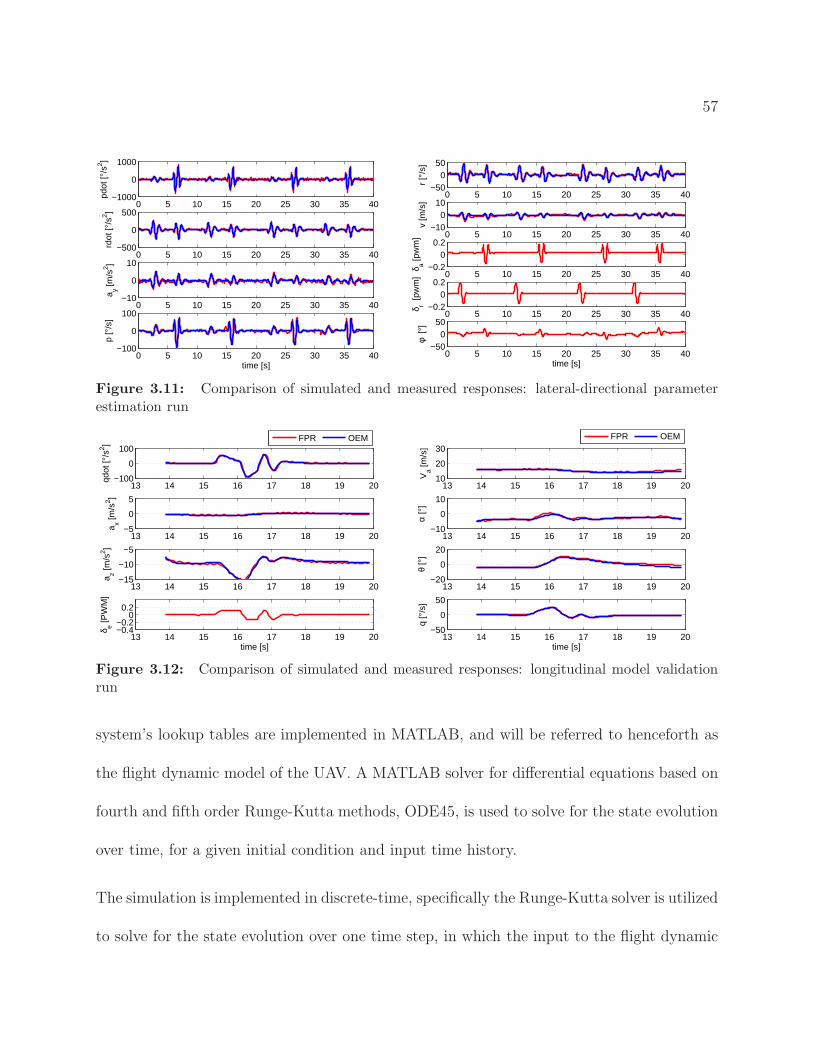
57

0 5 10 15 20 25 30 35 40−1000

0

1000

pdot

[°/s

2 ]

0 5 10 15 20 25 30 35 40−500

0

500

rdot

[°/s

2 ]

0 5 10 15 20 25 30 35 40−10

0

10

a y [m/s

2 ]

0 5 10 15 20 25 30 35 40−100

0

100

p [°

/s]

time [s]

0 5 10 15 20 25 30 35 40−50

050

r [°

/s]

0 5 10 15 20 25 30 35 40−10

010

v [m

/s]

0 5 10 15 20 25 30 35 40−0.2

00.2

δ a [pw

m]

0 5 10 15 20 25 30 35 40−0.2

00.2

δ r [pw

m]

0 5 10 15 20 25 30 35 40−50

050

φ [°

]

time [s]

Figure 3.11: Comparison of simulated and measured responses: lateral-directional parameterestimation run

13 14 15 16 17 18 19 20−100

0

100

qdot

[°/s

2 ]

13 14 15 16 17 18 19 20−5

0

5

a x [m/s

2 ]

13 14 15 16 17 18 19 20−15

−10

−5

a z [m/s

2 ]

13 14 15 16 17 18 19 20−0.4−0.2

00.2

δ e [PW

M]

time [s]

FPR OEM

13 14 15 16 17 18 19 2010

20

30

Va [m

/s]

13 14 15 16 17 18 19 20−10

0

10

α [°

]

13 14 15 16 17 18 19 20−20

0

20

θ [°

]

13 14 15 16 17 18 19 20−50

0

50

q [°

/s]

time [s]

FPR OEM

Figure 3.12: Comparison of simulated and measured responses: longitudinal model validationrun

system’s lookup tables are implemented in MATLAB, and will be referred to henceforth as

the flight dynamic model of the UAV. A MATLAB solver for differential equations based on

fourth and fifth order Runge-Kutta methods, ODE45, is used to solve for the state evolution

over time, for a given initial condition and input time history.

The simulation is implemented in discrete-time, specifically the Runge-Kutta solver is utilized

to solve for the state evolution over one time step, in which the input to the flight dynamic

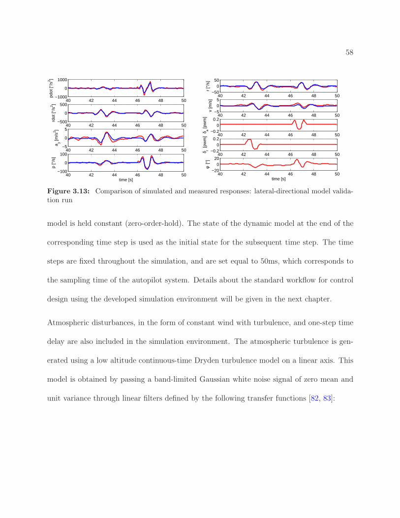
58

40 42 44 46 48 50−1000

0

1000

pdot

[°/s

2 ]

40 42 44 46 48 50−500

0

500

rdot

[°/s

2 ]

40 42 44 46 48 50−5

0

5

a y [m/s

2 ]

40 42 44 46 48 50−100

0

100

p [°

/s]

time [s]

40 42 44 46 48 50−50

050

r [°

/s]

40 42 44 46 48 50−5

05

v [m

/s]

40 42 44 46 48 50−0.2

00.2

δ a [pw

m]

40 42 44 46 48 50−0.2

00.2

δ r [pw

m]

40 42 44 46 48 50−20

020

φ [°

]

time [s]

Figure 3.13: Comparison of simulated and measured responses: lateral-directional model valida-tion run

model is held constant (zero-order-hold). The state of the dynamic model at the end of the

corresponding time step is used as the initial state for the subsequent time step. The time

steps are fixed throughout the simulation, and are set equal to 50ms, which corresponds to

the sampling time of the autopilot system. Details about the standard workflow for control

design using the developed simulation environment will be given in the next chapter.

Atmospheric disturbances, in the form of constant wind with turbulence, and one-step time

delay are also included in the simulation environment. The atmospheric turbulence is gen-

erated using a low altitude continuous-time Dryden turbulence model on a linear axis. This

model is obtained by passing a band-limited Gaussian white noise signal of zero mean and

unit variance through linear filters defined by the following transfer functions [82, 83]:

59

Hu(s) = σu

√

2VaπLu

1

s+ VaLu

, Hv(s) = σv

√

3VaπLv

s+ Va√3Lv

(

s+ VaLv

)2 , Hw(s) = σw

√

3VaπLw

s+ Va√3Lw

(

s+ VaLw

)2

(3.8)

where the coefficients in these equations are determined based on the flight and atmospheric

conditions, namely the airspeed (Va), the altitude above surface level (h in feet), and wind

speed at 6 m [20 ft] above surface level (W20). Specifically, the formulas for these coefficients

are given below:

Lu = Lw = h, Lv =h

(0.17 + 0.000823h)1.2

σw = 0.1W20, σu = σv =σw

(0.17 + 0.000823h)0.4

where the subscripts u, v, and w indicate the gust components in the body X, Y, and Z

axes, respectively. The Dryden turbulence model has appeared in numerous publications,

for instance, [82] and [83].

In this section we will use the simulation tool to examine how closely the derived flight

dynamic model describes the behavior of the UAV given certain commanded control inputs.

This analysis is achieved by comparing the simulation results to the actual flight test data.

Specifically, a couple of flight tests are chosen, and the initial conditions and time history of

the inputs during each test are used to drive the simulation model.

The first test data to be used in this verification process is obtained from a randomly chosen

part of the recorded flight data during a parameter estimation test. The data depicts a gentle

60

left turn maneuver performed by the UAV, that is the UAV transitions from a straight and

level flight into a steady left turn flight. The time histories of the inputs for this maneuver

are extracted and then used in the simulation to generate a similar maneuver shown in Figure

3.14. As evident from the figure, the simulated trajectory captures most of the features of

the actual flight trajectory.

0 20 40 60 800

10

20

30

40

50

60

Y [m]

X [m

]

flight testsimulation

0 1 2 3 4 5 6 7−50

0

50

p [°

/s]

0 1 2 3 4 5 6 7−50

0

50q

[°/s

]

0 1 2 3 4 5 6 7−50

0

50

time [s]

r [°

/s]

0 1 2 3 4 5 6 7

10

20

Va [m

/s]

0 1 2 3 4 5 6 7−10

010

α [°

]

0 1 2 3 4 5 6 7−10

010

time [s]

β [°

]

0 1 2 3 4 5 6 7−50

0

50

φ [°

]

0 1 2 3 4 5 6 7−10

010

θ [°

]

0 1 2 3 4 5 6 70

50

100

time [s]

ψ [°

]

Figure 3.14: Comparison of simulated and measured responses: a gentle left turn maneuver

To further assess the capability of the developed model to simulate aggressive maneuvers,

the following test is performed. The test utilizes data obtained during a Split-S maneuver.

This maneuver is executed when an airplane needs to make a 180 turn in a short amount of

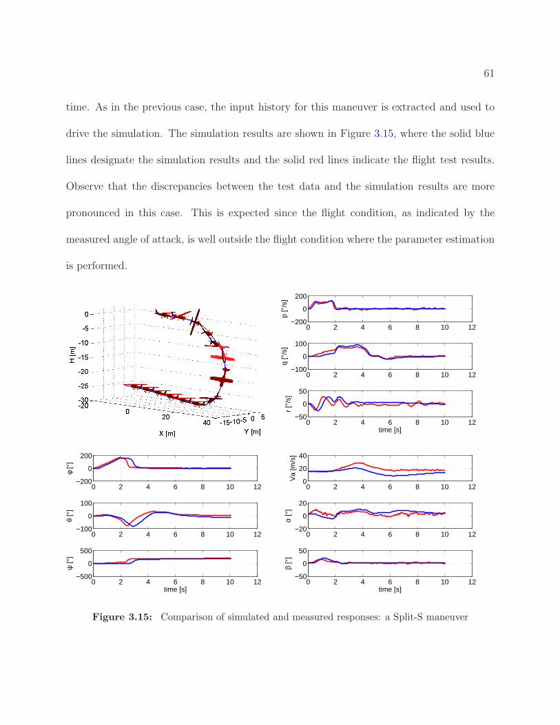
61

time. As in the previous case, the input history for this maneuver is extracted and used to

drive the simulation. The simulation results are shown in Figure 3.15, where the solid blue

lines designate the simulation results and the solid red lines indicate the flight test results.

Observe that the discrepancies between the test data and the simulation results are more

pronounced in this case. This is expected since the flight condition, as indicated by the

measured angle of attack, is well outside the flight condition where the parameter estimation

is performed.

0 2 4 6 8 10 12−200

0

200

p [°

/s]

0 2 4 6 8 10 12−100

0

100

q [°

/s]

0 2 4 6 8 10 12−50

0

50

r [°

/s]

time [s]

0 2 4 6 8 10 12−200

0

200

φ [°

]

0 2 4 6 8 10 12−100

0

100

θ [°

]

0 2 4 6 8 10 12−500

0

500

ψ [°

]

time [s]

0 2 4 6 8 10 120

20

40

Va

[m/s

]

0 2 4 6 8 10 12−20

0

20

α [°

]

0 2 4 6 8 10 12−50

0

50

β [°

]

time [s]

Figure 3.15: Comparison of simulated and measured responses: a Split-S maneuver

Chapter 4

Control System Design, Simulation,

and Flight Testing

In this chapter, we design several controllers to be implemented on the testbed. Specifically,

we are interested in using output feedback controllers with ℓ2-induced norm performance

measure to track real-time trajectories. We assume that the desired trajectories are generated

from a library of pre-specified motion primitives using some primitive-based motion planner.

The library usually consists of trim conditions and transitions between trim conditions.

Using the flight dynamic model derived in the previous chapter, the motion primitives can

be generated off-line using the aforementioned simulation environment. The trim conditions

can be obtained easily by solving for the equilibrium points of the nonlinear mathematical

model. The transition maneuvers are not as easy to generate in general, but there are several

methods that can be utilized for this purpose. One method entails formulating the problem

62

63

as a nonlinear optimization problem and then using algorithms such as DIDO [84] to solve it.

Alternatively, the maneuvers can be obtained by recording pilot inputs and corresponding

system responses during an actual flight [41]. In this dissertation, we will use simple feedback

control to obtain transition maneuvers between trim conditions and utilize recorded pilot

input to generate the Split-S maneuver.

The controllers will be synthesized based on linearized models about motion primitives.

Linearizing the nonlinear dynamics about a trim condition results in a linear time-invariant

(LTI) system, whereas linearizing the nonlinear dynamics about a transition maneuver results

in a finite-horizon linear time-varying (LTV) system.

4.1 Preliminaries

4.1.1 Notation

The notation is quite standard. We denote the set of real n×m matrices by Rn×m. IfMi is a

sequence of matrices, then diag(Si) denotes their block-diagonal augmentation. We use In to

denote an n×n identity matrix and 0n×m to denote an n×m zero matrix. The transpose of a

matrix X is written XT . Given a symmetric matrix X , we use X ≺ 0 to mean it is negative

definite. The normed space of square summable vector-valued sequences is denoted by ℓ2.

It consists of elements x = (x0, x1, x2, . . .), with xk ∈ Rn for some n, having a finite 2-norm

‖x‖ℓ2 defined by ‖x‖2ℓ2 =∑∞

k=0‖xk‖22 < ∞, where ‖xk‖

22 = xTk xk, that is, ‖·‖2 denotes the

64

Euclidean norm. We use the notation ‖P‖ℓ2→ℓ2 to denote the ℓ2 induced norm of a bounded

linear mapping P on ℓ2.

4.1.2 Control Synthesis

This work makes use of the LMI-based control synthesis techniques developed in [37, 38, 20]

for discrete-time LTI systems, finite horizon systems, and linear systems with uncertain

initial conditions, respectively. These techniques will be used to design switched controllers

for the regulation of the UAV about concatenated trajectories. The performance measure for

designing the optimal controllers is the ℓ2 induced norm in the case of plants with zero initial

conditions and the square ℓ2 induced norm in the case of uncertain initial conditions. The

first two subsections give procedures for constructing optimal controllers for finite horizon

and LTI systems with zero initial conditions, whereas the last subsection considers LTI plants

with uncertain initial states.

Finite horizon systems

Consider a finite horizon linear discrete-time plant G, described by the following state-space

equation:

xk+1

zk

yk

=

Ak B1k B2k

C1k D11k D12k

C2k D21k 0

xk

dk

δk

, x0 = 0, (4.1)

65

K

Gz d

y δ

Figure 4.1: Closed-loop system

for k = 0, 1, . . . , h − 1, with h designating the finite horizon length. The signal xk ∈ Rn

is the error between the actual and reference values of the state vector at discrete instant

k, namely xk = xk − xr,k, where the subscript r refers to the reference data. Similarly,

δk = δk − δr,k ∈ Rnδ and yk = yk − yr,k ∈ R

ny , where δk and yk denote the applied control

input and the measurements at time k, respectively, with δr,k and yr,k indicating the reference

values. The signals dk ∈ Rnd and zk ∈ R

nz denote the exogenous disturbances and errors,

respectively. The goal is to design a feedback controller K, defined by the state-space

equation

xKk+1

δk

=

AKk BKk

CKk DK

k

xKk

yk

, xK0 = 0, (4.2)

with xKk ∈ Rn, such that the closed-loop system in Figure 4.1 is asymptotically stable and

‖d 7→ z‖ℓ2→ℓ2 < γmin, where γmin is the minimum achievable ℓ2-gain performance level up to

a certain tolerance.

The procedure for constructing the feedback controller K is based on the work in [37, 38]

and is summarized as follows:

1. Solve the following semidefinite programming optimization problem for the matrix

sequences Rk and Sk, for k = 0, 1, . . . , h− 1, and the scalar γmin (which is the square

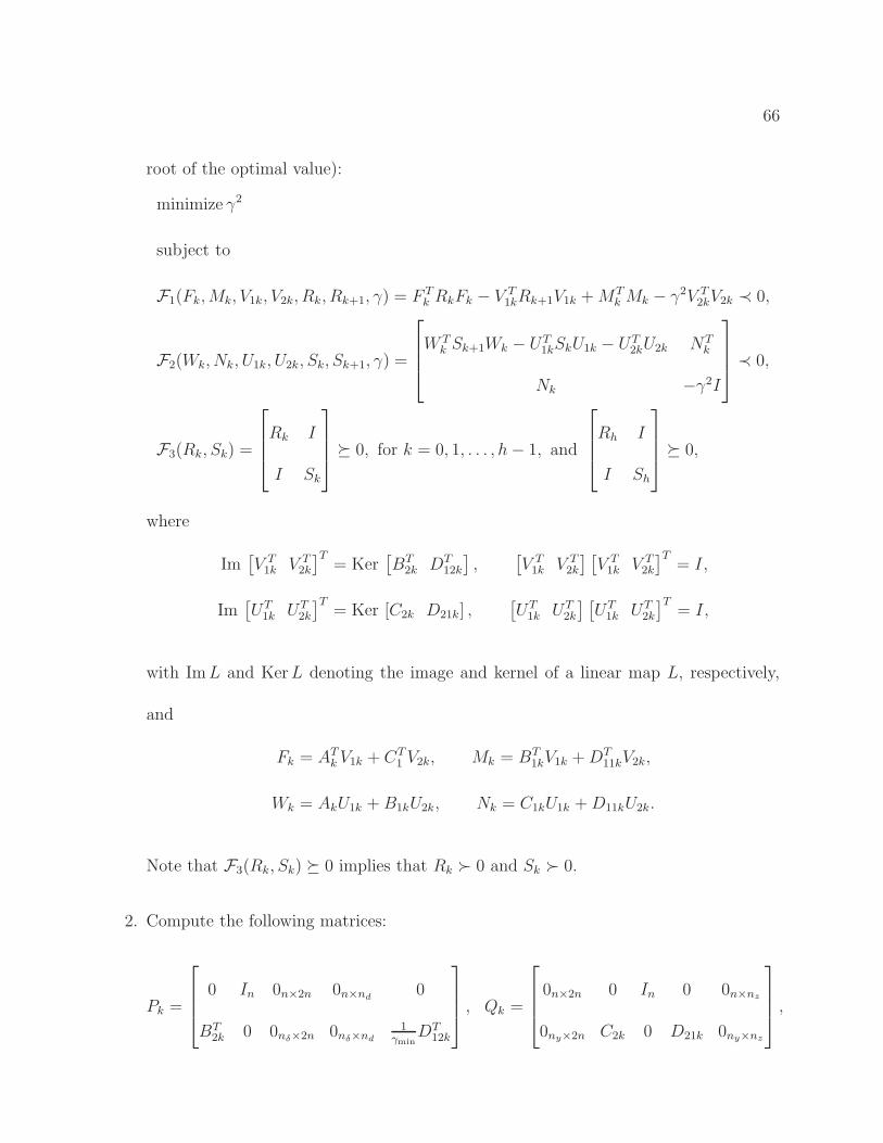
66

root of the optimal value):

minimize γ2

subject to

F1(Fk,Mk, V1k, V2k, Rk, Rk+1, γ) = F Tk RkFk − V T

1kRk+1V1k +MTk Mk − γ2V T

2kV2k ≺ 0,

F2(Wk, Nk, U1k, U2k, Sk, Sk+1, γ) =

W Tk Sk+1Wk − UT

1kSkU1k − UT2kU2k NT

k

Nk −γ2I

≺ 0,

F3(Rk, Sk) =

Rk I

I Sk

0, for k = 0, 1, . . . , h− 1, and

Rh I

I Sh

0,

where

Im[

V T1k V T

2k

]T= Ker

[

BT2k DT

12k

]

,[

V T1k V T

2k

] [

V T1k V T

2k

]T= I,

Im[

UT1k UT

2k

]T= Ker [C2k D21k] ,

[

UT1k UT

2k

] [

UT1k UT

2k

]T= I,

with ImL and KerL denoting the image and kernel of a linear map L, respectively,

and

Fk = ATk V1k + CT1 V2k, Mk = BT

1kV1k +DT11kV2k,

Wk = AkU1k +B1kU2k, Nk = C1kU1k +D11kU2k.

Note that F3(Rk, Sk) 0 implies that Rk ≻ 0 and Sk ≻ 0.

2. Compute the following matrices:

Pk =

0 In 0n×2n 0n×nd0

BT2k 0 0nδ×2n 0nδ×nd

1γmin

DT12k

, Qk =

0n×2n 0 In 0 0n×nz

0ny×2n C2k 0 D21k 0ny×nz

,

67

Hk =

−Rk+1 −Ek+1 Ak 0 B1k 0

−ETk+1 −In 0 0 0 0

ATk 0 −Sk SkEk 0 1γmin

CT1k

0 0 ETk Sk −In − ET

k SkEk 0 0

BT1k 0 0 0 −Ind

1γmin

DT11k

0 0 1γmin

C1k 0 1γmin

D11k −Inz

,

where Ek =(

Rk − S−1k

)1

2 .

3. Obtain the state-space matrices of the controller, Jk =

AKk BKk

CKk DK

k

, by solving the

following LMI:

Hk +QTk J

Tk Pk + P T

k JkQk ≺ 0,

for each k ∈ 0, 1, . . . , h − 1. Note that the Matlab command basiclmi is useful in

this regard.

It is also possible to derive explicit controller formulas based on the results of [37] or [85];

see, for instance, the algorithm derived in [86, 22] for nonstationary linear parameter-varying

systems.

Linear time-invariant systems

Suppose the state-space matrices in (4.1) are constant, and hence the plant G in this case

is a discrete-time LTI plant. The synthesis objective is the same as in the finite horizon

68

case in that we seek to design a feedback controller K, which is LTI in this case, defined

by the state-space equation in (4.2) with the subscript k in the notation of the controller

state-space matrices dropped, such that the closed-loop system is asymptotically stable and

‖d 7→ z‖ℓ2→ℓ2 < γmin. The procedure for designing the optimal H∞ controller is given in [37]

and included next for completeness:

1. Solve the following semidefinite program for the scalar γmin and the matrices R and S:

minimizeγ2

subject to

F1(F,M, V1, V2, R, R, γ) ≺ 0, F2(W,N,U1, U2, S, S, γ) ≺ 0, F3(R, S) 0.

Note that the synthesis solutions are constant in this case, that is, Rk+1 = Rk = R

and Sk+1 = Sk = S, and so are the state-space matrices, hence the omittance of the

subscript k.

2. Compute the state-space matrices of the controller by solving the following LMI for J :

H +QTJTP + P TJQ ≺ 0,

where again, for clarity, Ek+1 = Ek = E, Rk+1 = Rk = R, and Sk = S.

LTI systems with uncertain initial states

Given the LTI plant from the previous subsection, suppose that some of the state variables

have uncertain, nonzero initial values. Namely, x0 6= 0, but rather x0 = Λx0, where Λ is a

constant n×m matrix for some m and x0 is an uncertain, norm-bounded m-entry vector. In

69

this case, the control synthesis objective is to find a discrete-time linear feedback controller

K that results in a stable closed-loop system, which satisfies the performance inequality

‖(x0, w) 7→ z‖sq := sup‖x0‖2≤1, ‖w‖ℓ2≤1

‖z‖ℓ2 < γmin,

where ‖·‖sq denotes the square ℓ2 induced norm, and γmin is the minimum achievable per-

formance level up to a certain tolerance by the considered class of linear controllers. As

discussed in [20], it is conceivable that an N -eventually time-invariant controller, for some

integer N ≥ 1, could provide an improved performance over an LTI one in general. An

LTV controller is N -eventually time-invariant controller if each of its state-space matrix se-

quences is N -eventually time-invariant; for instance, the sequence AKk would be of the form

AK0 , AK1 , . . . , A

KN−1, A

KN , A

KN , A

KN , . . .. The procedure for constructing an optimalN -eventually

times-invariant controller is given in [20] and summarized as follows:

1. Solve the following semidefinite program for the matrix sequences Rk and Sk, for

k = 0, 1, . . . , N , and the optimal value γmin:

70

minimize γ

subject to e+ f1 + f2 < 2γ, ΛTS0Λ ≺ f1I,

V1

V2

T

A B1

C1 D11

Rk 0

0 pI

A B1

C1 D11

T

−

Rk+1 0

0 eI

V1

V2

≺ 0,

U1

U2

T

A B1

C1 D11

T

Sk+1 0

0 tI

A B1

C1 D11

−

Sk 0

0 f2I

U1

U2

≺ 0,

Rk I

I Sk

0,

p 1

1 f2

0,

t 1

1 e

0,

for k = 0, 1, . . . , N , with RN+1 = RN and SN+1 = SN .

2. Construct an N -eventually time-invariant controller (with zero initial condition) from

the synthesis solutions by solving the following LMI:

Hk + QTJTk P + P TJkQ ≺ 0,

for k = 0, 1, . . . , N , where Hk, P , and Q are defined as

P =

0 In 0n×2n 0n×nd0

BT2 0 0nδ×2n 0nδ×nd

e−1

2DT12

, Q =

0n×2n 0 In 0 0n×nz

0ny×2n C2 0 f− 1

2

2 D21 0ny×nz

,

71

Hk =

−Rk+1 −Ek+1 A 0 f− 1

2

2 B1 0

−ETk+1 −In 0 0 0 0

AT 0 −Sk SkEk 0 e−1

2CT1

0 0 ETk Sk −In − ET

k SkEk 0 0

f− 1

2

2 BT1 0 0 0 −Ind

(ef2)− 1

2DT11

0 0 e−1

2C1 0 (ef2)− 1

2D11 −Inz

.

4.1.3 Plant Model Formulation

The controllers in this chapter are synthesized based on linearized plant models. This subsec-

tion demonstrates how these linearized models are formulated. As the servomotor response

is much faster than the dynamic response of the aircraft, we may neglect the effect of the

servomotor dynamics in the control design process to reduce the computational complexity

of the control synthesis problem. The servomotor models, however, will be incorporated in

the simulation environment.

Notice that the heading angle ψ only appears in the equations of motion (3.3) correspond-

ing to the position vector P . Then, when linearizing this equation about some reference

trajectory, the resultant linearized equation will depend on the initial reference heading ori-

entation. For example, if the reference trajectory is a straight and level trim trajectory,

then we will obtain different linearized models for different heading orientations. This is not

favorable for the control approaches used in this work as we will then have to design different

controllers for these different linearized models when we know intuitively that the same con-

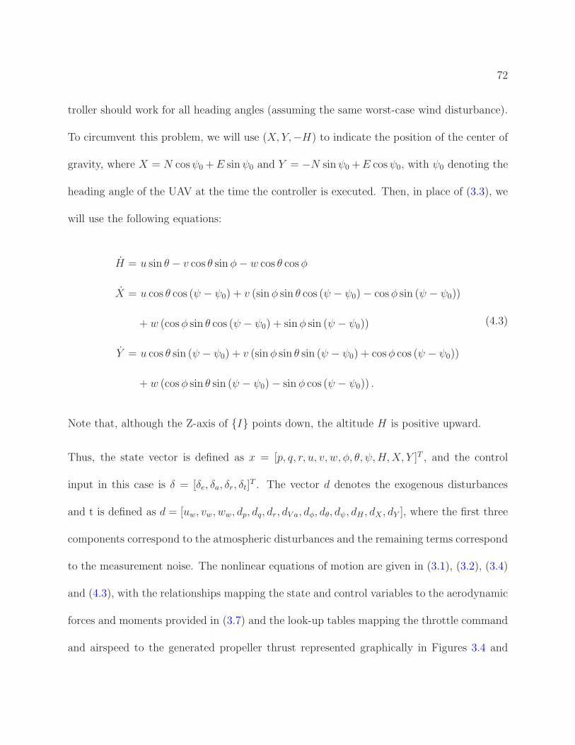
72

troller should work for all heading angles (assuming the same worst-case wind disturbance).

To circumvent this problem, we will use (X, Y,−H) to indicate the position of the center of

gravity, where X = N cosψ0 +E sinψ0 and Y = −N sinψ0 +E cosψ0, with ψ0 denoting the

heading angle of the UAV at the time the controller is executed. Then, in place of (3.3), we

will use the following equations:

H = u sin θ − v cos θ sin φ− w cos θ cosφ

X = u cos θ cos (ψ − ψ0) + v (sinφ sin θ cos (ψ − ψ0)− cosφ sin (ψ − ψ0))

+ w (cosφ sin θ cos (ψ − ψ0) + sinφ sin (ψ − ψ0))

Y = u cos θ sin (ψ − ψ0) + v (sinφ sin θ sin (ψ − ψ0) + cosφ cos (ψ − ψ0))

+ w (cosφ sin θ sin (ψ − ψ0)− sin φ cos (ψ − ψ0)) .

(4.3)

Note that, although the Z-axis of I points down, the altitude H is positive upward.

Thus, the state vector is defined as x = [p, q, r, u, v, w, φ, θ, ψ,H,X, Y ]T , and the control

input in this case is δ = [δe, δa, δr, δt]T . The vector d denotes the exogenous disturbances

and t is defined as d = [uw, vw, ww, dp, dq, dr, dV a, dφ, dθ, dψ, dH , dX , dY ], where the first three

components correspond to the atmospheric disturbances and the remaining terms correspond

to the measurement noise. The nonlinear equations of motion are given in (3.1), (3.2), (3.4)

and (4.3), with the relationships mapping the state and control variables to the aerodynamic

forces and moments provided in (3.7) and the look-up tables mapping the throttle command

and airspeed to the generated propeller thrust represented graphically in Figures 3.4 and

73

3.5. These equations of motion can be expressed in state-space form as x = f(x, δ, d),

where f(·, ·, ·) is defined in the obvious way. The following measurements are assumed to be

available at a sampling rate of 20Hz:

y = h(x, d) = [p, q, r, Va, φ, θ, ψ,H,X, Y ]T +D21 d,

where D21 = [010×3 diag(0.5, 0.5, 0.5, 2, 0.01, 0.01, 0.01, 2, 2, 2)] is chosen based on the sensor

noise characteristics and some expected uncertainties.

Suppose that the control objective is to design a controller that would force the system

to track closely the reference trajectory (xr, δr, dr), where dr = 0. Then, linearizing the

nonlinear system equation about this reference trajectory results in the following continuous-

time LTV state-space equations:

˙x(t) = Ac(t)x(t) +B1c(t)d(t) +B2c(t)δ(t),

y(t) = C2c(t)x(t) +D21d(t),

where t is continuous time, x = x− xr, δ = δ − δr, y = y − yr, and

Ac =∂f

∂x

∣

∣

∣

∣

(xr,δr ,dr)

B1c =∂f

∂d

∣

∣

∣

∣

(xr ,δr,dr)

B2c =∂f

∂δ

∣

∣

∣

∣

(xr ,δr,dr)

C2c =∂h

∂x

∣

∣

∣

∣

(xr ,dr)

with dr = 0 as aforementioned. Note that, since f(x, δ, d) depends on the first three compo-

nents of d only, namely Vw = [uw, vw, ww]T , the matrix-valued function B1c(t) is of the form

B1c(t) = [B1w(t) 012×10], where B1w =∂f

∂Vw

∣

∣

∣

∣

(xr ,δr,dr)

with dr and specifically Vwr set to zero.

The Jacobian matrices are computed using the small perturbation method because of the

use of the Javaprop look-up tables.

74

Discretizing the previous equations using zero-order hold sampling with sampling time τ =

0.05 s yields the following discrete-time LTV model:

xk+1 = Akxk +B1kdk +B2kδk,

yk = C2kxk +D21dk,

where xk = x(kτ), δk = δ(kτ), yk = y(kτ), C2k = C2c(kτ) for integers k ≥ 0, Ak =

Φ((k + 1)τ, kτ), with Φ(·, ·) being the state transition matrix, and, for i = 1, 2,

Bik =

∫ (k+1)τ

kτ

Φ ((k + 1)τ, s)Bic(s)ds.

If the reference trajectory is a maneuver defined over a finite time interval, then the resulting

linearized model will be a finite-horizon model. In the event of a trim reference trajectory,

the linearized model will be LTI, in which case all the state-space matrices will be constant

and the state transition matrix Φ (t2, t1) will simply be the matrix exponential eA(t2−t1).

The performance output z will be defined in the following sections as we consider different

trajectory tracking problems.

4.2 Tracking of a Figure-8 Trajectory

We now implement the approaches discussed in Section 4.1.2 to control the Telemaster UAV

about a reference trajectory generated (in real-time) from a library of pre-specified motion

primitives. Specifically, a standard H∞ controller and a switched UIC controller will be

designed and tested in simulation and on the actual UAV. The section is divided into three

75

subsections: the first gives the motion primitives that will be used in generating the reference

trajectory; the second presents the control systems; and the third provides the simulation

and flight testing results, along with some interesting observations.

4.2.1 Motion primitives

A motion primitive is a dynamically feasible trajectory that can be obtained experimentally

from flight tests or, as is the case in this chapter, numerically from the nonlinear equations

of motion. Specifically, the transition maneuvers in our case will be obtained by simulation,

as discussed later, and the trim conditions will be generated using the MATLAB command

fminsearch.

We construct a library of motion primitives that consists of three equilibrium (trimmed)

conditions and four transition maneuvers. The primitives are judiciously chosen to achieve

the desired maneuverability. The trim conditions considered correspond to straight and level

flight (SSLF), steady right turn (SRT), and steady left turn (SLT), all of which obtained at

a nominal airspeed of 15m/s and an altitude of 580m (above sea level). Furthermore, the

steady turns are performed at a bank angle of 30 for the clockwise direction and −30 for

the counter-clockwise direction. The required bank angle and airspeed are passed on to a

trimming routine in the simulation environment. The trim condition search process is based

on the Nelder-Mead simplex algorithm, which can be invoked by calling the fminsearch

command in MATLAB. Table 4.1 gives the values of the states and control inputs corre-

76

Table 4.1: Trim conditions used in generating the figure-8 trajectory

Trim Condition p q r u v w H[rad/s] [rad/s] [rad/s] [m/s] [m/s] [m/s] [m]

straight and level 0.0000 0.0000 0.0000 15.0 1.0 -0.2 580.0steady right turn -0.0131 0.1882 0.3260 15.0 0.9 0.1 580.0steady left turn -0.0120 0.1882 -0.3259 15.0 1.1 0.1 580.0Trim Condition φ θ ψ δe δa δr δt

[rad] [rad] [rad] [pwm] [pwm] [pwm] [pwm]straight and level 0.0000 -0.0132 0.0000 0.0045 -0.0574 -0.0525 0.3956steady right turn 0.5236 0.0347 0.0000 0.0471 -0.0777 -0.0851 0.4135steady left turn -0.5236 -0.0319 0.0000 0.0469 -0.0406 -0.0167 0.4135

sponding to the aforementioned trim conditions. Note that, in all the tables and figures

herein, the control surface deflections are given in terms of the deviations from the reference

pwm values. In the case of the elevator, aileron, and rudder, the reference value is 1.5ms,

which corresponds to approximately zero deflection. As for the throttle, the reference value

is 1.1ms and corresponds to the minimum possible throttle deflection.

The transition maneuvers in our case begin and end at trim conditions. As mentioned before,

these maneuvers can be generated using several methods. For generating the transition ma-

neuvers in this work, linear feedback controllers are used. Specifically, the nonlinear system

(sans actuator dynamics) is linearized about the trim conditions and then the resulting LTI

models are discretized using zero-order-hold sampling with a sampling time of 0.05 s, which

is the sampling time of the autopilot hardware onboard the UAV. Given these linearized

models, we then design a Linear Quadratic Regulator (LQR) for each of the discrete-time

linear models using the MATLAB command dlqr. In the LQR design, we evenly penalize

all the states and inputs. Then, for example, to generate the straight and level flight to

77

steady right turn maneuver, the simulation is set to start from the straight and level trim

condition. The feedback controller is set to use the LQR that is obtained for the steady right

turn. The reference (equilibrium) state and control values for this controller correspond to

the steady right turn. The simulated maneuver is truncated when the values of the states

are relatively close to the target ones. Note that this simple method may not work when the

two trim conditions are relatively far apart.

Following this approach, we end up with four transition maneuvers, namely straight-to-

right, right-to-straight, straight-to-left, and left-to-straight maneuvers. The time span of

each transition is constant and equal to about 5 s (100 sampling points). To generate the

figure-8 path, the amount of time the UAV flies along each trim trajectory (i.e., coasting

time) is varied to result in the desired geometric path with the errors in the X and Y

positions at transition-to-trim connection points being less than 0.5m. Figure 4.2 shows the

motion primitives composing the library and the desired reference trajectory generated from

these primitives. As can be seen from the figure, the angle of attack at trim is not zero;

the reason is that the required lift is not achieved at zero angle of attack. In addition, the

non-zero sideslip follows from the asymmetry of the aircraft, which is due to manufacturing

defects and/or propeller effects.

78

−100 −50 0 50 100 150

−100

−50

0

50

100

Y [m]

X [m

]

SSLFSSLF−SRTSRTSRT−SSLFSSLFSSLF−SLTSLTSLT−SSLF

0 5 10 15 20 25 30 35 40−50

0

50

p [d

eg/s

]

0 5 10 15 20 25 30 35 40−20

0

20

q [d

eg/s

]

0 5 10 15 20 25 30 35 40−50

0

50

r [d

eg/s

]

time [s]

0 5 10 15 20 25 30 35 40−50

0

50

φ [d

eg]

0 5 10 15 20 25 30 35 40−20

0

20

θ [d

eg]

0 5 10 15 20 25 30 35 400

100200300

ψ [d

eg]

time [s]

0 5 10 15 20 25 30 35 40575

580

585

H [m

]

0 5 10 15 20 25 30 35 40−200

0

200

X [m

]

0 5 10 15 20 25 30 35 40−100

0

100

Y [m

]

time [s]

0 5 10 15 20 25 30 35 4012

14

16

Va [m

/s]

0 5 10 15 20 25 30 35 40−2

0

2

α [d

eg]

0 5 10 15 20 25 30 35 400

5

10

β [d

eg]

time [s]

0 5 10 15 20 25 30 35 400

0.05

0.1

δ e [pw

m]

0 5 10 15 20 25 30 35 40−0.2

0

0.2

δ a [pw

m]

0 5 10 15 20 25 30 35 40−0.1

0

0.1

δ r [pw

m]

0 5 10 15 20 25 30 35 40

0.350.4

0.45

δ t [pw

m]

time [s]

Figure 4.2: Reference trajectory of a figure-8 pattern obtained by concatenating seven motionprimitives

79

4.2.2 Control design

We now design two controllers based on the aforementioned library of motion primitives:

a standard H∞ controller and a switched UIC controller. Although the controllers will

be ultimately used to track the figure-8 trajectory, the only assumption made about the

trajectory to be tracked in designing these controllers is that this trajectory will be generated

in real-time by concatenating primitives from the library.

Standard H∞ Controller

As the steady turn trim trajectories and transition maneuvers do not deviate significantly

from the straight and level flight, it is conceivable that a properly designed standard H∞

controller, synthesised based on a linearized plant model about the straight and level flight,

should work reasonably well. The linearized state equation would then be ∆x = A∆x +

B1d + B2∆δ, where ∆x = x − xtrim and ∆δ = δ − δtrim, with (xtrim, δtrim) designating the

state and control input corresponding to the straight and level trim trajectory. We may also

write ∆xr ≈ A∆xr+B2∆δr, for “small” ∆xr = xr−xtrim and ∆δr = δr−δtrim, where (xr, δr)

denote the state and control input corresponding to the trajectory to be tracked. Then, as

x = x−xr = ∆x−∆xr and δ = δ−δr = ∆δ−∆δr, the plant state equation can be expressed

as ˙x = Ax + B1d + B2δ. The rest of the plant formulation follows the description given in

Section 4.1.3, with the performance output z judiciously chosen as

80

z =[0.2 p, 0.2 q, 0.2 r, 0.1 u, 0.01 φ, 0.01 θ, 0.01 ψ, 0.01 H, 0.05 X, 0.01 Y ,

0.4 δe, 0.4 δa, 0.6 δr, 1.0 δt]T .

The control design follows the procedure outlined in Section 4.1.2. All computations are

carried out on an ASUS laptop with an Intel dual-core Pentium M2020 2.4 GHz processor,

4 GB RAM, and 64-bit Windows 8 operating system running 64-bit MATLAB R2011a. The

semidefinite programs are solved using YALMIP/SDPT3-v4 [87, 88]. The elapsed (i.e., wall

clock) time to solve for the minimum achievable ℓ2-gain performance level γ is about 1 s

(CPU time = 0.78 s). The optimal value, which is found to be γmin = 0.33, is relaxed to 0.35

in order to obtain a satisfactory controller performance.

Switched UIC Controller

The switched UIC controller consists of three N -eventually time-invariant subcontrollers

synthesised separately based on discrete-time linear models with uncertain initial conditions,

following the procedure in Section 4.1.2. The three linear plant models in question are

obtained by linearizing the equations of motion about the straight and level, steady right

turn, and steady left turn flights, and are formulated as described in Section 4.1.3.

Choosing the exogenous errors z that would result in a satisfactory controller performance

has proved to be a bit more challenging in this case. Namely, if we are to use the same penalty

weights as before, the resulting controller tends to fail under a small amount of atmospheric

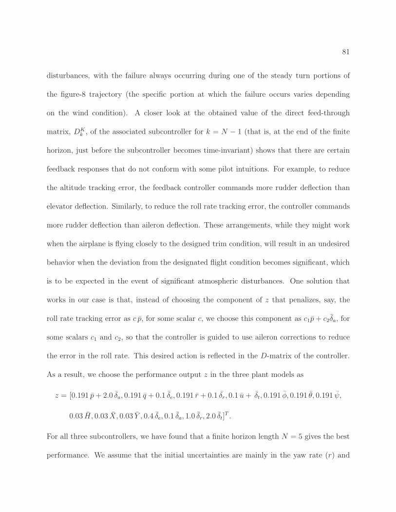
81

disturbances, with the failure always occurring during one of the steady turn portions of

the figure-8 trajectory (the specific portion at which the failure occurs varies depending

on the wind condition). A closer look at the obtained value of the direct feed-through

matrix, DKk , of the associated subcontroller for k = N − 1 (that is, at the end of the finite

horizon, just before the subcontroller becomes time-invariant) shows that there are certain

feedback responses that do not conform with some pilot intuitions. For example, to reduce

the altitude tracking error, the feedback controller commands more rudder deflection than

elevator deflection. Similarly, to reduce the roll rate tracking error, the controller commands

more rudder deflection than aileron deflection. These arrangements, while they might work

when the airplane is flying closely to the designed trim condition, will result in an undesired

behavior when the deviation from the designated flight condition becomes significant, which

is to be expected in the event of significant atmospheric disturbances. One solution that

works in our case is that, instead of choosing the component of z that penalizes, say, the

roll rate tracking error as c p, for some scalar c, we choose this component as c1p+ c2δa, for

some scalars c1 and c2, so that the controller is guided to use aileron corrections to reduce

the error in the roll rate. This desired action is reflected in the D-matrix of the controller.

As a result, we choose the performance output z in the three plant models as

z = [0.191 p+ 2.0 δa, 0.191 q + 0.1 δe, 0.191 r + 0.1 δr, 0.1 u+ δt, 0.191 φ, 0.191 θ, 0.191 ψ,

0.03 H, 0.03 X, 0.03 Y , 0.4 δe, 0.1 δa, 1.0 δr, 2.0 δt]T .

For all three subcontrollers, we have found that a finite horizon length N = 5 gives the best

performance. We assume that the initial uncertainties are mainly in the yaw rate (r) and

82

bank angle (φ). Accordingly, with x0 = Λ [r, φ]T , we define the scaling matrix Λ as

Λ =

0 0 0.1 0 0 0 0 0 0 0 0 0

0 0 0 0 0 0 0.5 0 0 0 0 0

T

.

The minimum achievable performance level is γmin ≈ 1.27 for each of the three 5-eventually

time-invariant subcontrollers; this value is then relaxed to 1.3 in order to obtain numerically

well-conditioned solutions. The wall clock time to find the optimal solution is about 16 s

(CPU time ≈ 15 s) for the straight and level flight case and about 9.5 s (CPU time ≈ 8.5 s)

for each of the steady turn cases. As for the implementation of the switched controller, we

start by executing the subcontroller associated with the steady straight and level flight; then,

when it is time to implement the appropriate transition maneuver to make a steady right

turn, the subcontroller associated with the steady right turn is activated and used to force

the system to track the transition maneuver followed by the steady right turn, and so on.

4.2.3 Simulation and flight test results

The performance of each designed controller is first analyzed through simulation in a realistic

operational environment to ensure that the controller can be safely implemented on the

actual test platform. As opposed to merely following a geometric path, the control goal in

this work is to ensure, among other things, reasonably accurate tracking of the reference

time histories of the inertial X-, Y -, and H-positions. For this reason, we define two metrics

to quantitatively compare the position tracking performance of the two controllers, namely

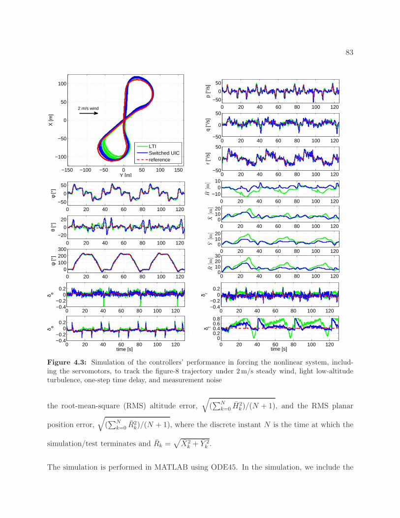
83

−150 −100 −50 0 50 100 150

−100

−50

0

50

100

X [m

]

Y [m]

LTISwitched UICreference

2 m/s wind 0 20 40 60 80 100 120−50

0

50

p [°

/s]

0 20 40 60 80 100 120−50

0

50

q [°

/s]

0 20 40 60 80 100 120−50

0

50

time [s]

r [°

/s]

0 20 40 60 80 100 120−50

0

50

φ [°

]

0 20 40 60 80 100 120

−20

0

20

θ [°

]

0 20 40 60 80 100 1200

100200300

ψ [°

]

0 20 40 60 80 100 120−10

010

H[m

]

0 20 40 60 80 100 1200

1020

X[m

]

0 20 40 60 80 100 1200

1020

Y[m

]

0 20 40 60 80 100 1200

102030

R[m

]

time [s]

0 20 40 60 80 100 120−0.4−0.2

00.2

δ e

0 20 40 60 80 100 120−0.4−0.2

00.2

δ a

time [s]

0 20 40 60 80 100 120−0.4−0.2

00.2

δ r

0 20 40 60 80 100 1200

0.20.40.60.8

δ t

time [s]

Figure 4.3: Simulation of the controllers’ performance in forcing the nonlinear system, includ-ing the servomotors, to track the figure-8 trajectory under 2m/s steady wind, light low-altitudeturbulence, one-step time delay, and measurement noise

the root-mean-square (RMS) altitude error,√

(∑N

k=0 H2k)/(N + 1), and the RMS planar

position error,√

(∑N

k=0 R2k)/(N + 1), where the discrete instant N is the time at which the

simulation/test terminates and Rk =√

X2k + Y 2

k .

The simulation is performed in MATLAB using ODE45. In the simulation, we include the

84

servomotor dynamics as well as a one-step time delay, whereby the control input computed

at discrete time k is applied at time k + 1. We impose lower and upper saturation limits on

the four commanded control (pwm) signals of 1.1ms and 1.9ms, respectively. The system is

also subjected to zero-mean Gaussian measurement noise, with standard deviations 0.5 rad/s

for p, q, r, 2m/s for Va, 0.01 rad for φ, θ, ψ, and 2m for H , X , Y (the same as the entries of

the D21 matrix). As for wind disturbances, a constant wind of 2m/s is applied, along with

the corresponding turbulence generated using the low-altitude Dryden turbulence model [83]

(specifically, airspeed used in Dryden model is 15m/s, altitude above surface level is 80m,

and wind speed at 6m [20 ft] above surface level is W20 = 2m/s). For each controller, the

same measurement noise and atmospheric turbulence are used, and the simulation is run

long enough for the UAV to track the figure-8 trajectory ten times.

Figure 4.3 shows the simulation results; for clarity, we only include the state and control

time histories for three traversals of the figure-8 trajectory, but the displayed results are

representative of the complete simulation run. The RMS planar position error is 9.76m for

the standard H∞ controller and 7.11m for the switched UIC controller. The RMS altitude

error is 5.12m for the H∞ controller and 2.07m for the switched controller. Note that

the control inputs vary rapidly because of the excessive sensor noise used in the simulation

environment to account for sensor inaccuracies. In general, both controllers perform well,

with the switched UIC controller clearly outperforming the standard H∞ one in tracking the

reference inertial positions, especially the altitude.

The controllers are also implemented on the Telemaster platform. The flight tests are per-

85

−150 −100 −50 0 50 100 150

−100

−50

0

50

100

X [m

]

Y [m]

referenceLTISwitched UIC

1−3 m/swind 0 20 40 60 80 100 120

−500

50

p [°

/s]

0 20 40 60 80 100 120−50

0

50

q [°

/s]

0 20 40 60 80 100 120−50

0

50

r [°

/s]

0 20 40 60 80 100 120

−500

50

φ [°

]

0 20 40 60 80 100 120−40−20

02040

θ [°

]

0 20 40 60 80 100 120

0100200300

ψ [°

]

0 20 40 60 80 100 120−30−20−10

010

H[m

]

0 20 40 60 80 100 120−20

020

X[m

]

0 20 40 60 80 100 120−20

020

Y[m

]

0 20 40 60 80 100 1200

20

40

R[m

]

time [s]

0 20 40 60 80 100 120−0.4−0.2

00.2

δ e

0 20 40 60 80 100 120−0.4−0.2

00.2

δ a

time [s]

0 20 40 60 80 100 120−0.4−0.2

00.2

δ r

0 20 40 60 80 100 1200

0.20.40.60.8

δ t

time [s]time [s]

Figure 4.4: Controller tracking performance in flight tests

formed on a calm-air day, where the wind speed is 1-3m/s based on data from a nearby

on-ground station. Each test is performed in a separate flight, with a battery change taking

place in-between tests. The results from both tests are given in Figure 4.4. Note that, since

the tests are run in separate flights, the wind disturbances differ from test to test, and hence

any performance comparison between the two controllers should be construed qualitatively.

86

With this said, it is observed that the results from the flight tests are in agreement with

the simulation results in that both controllers perform comparably well. The values of the

RMS planar position error are 11.46m and 10.25m, and those of the RMS altitude error are

7.44m and 3.16m, for the standard H∞ and switched UIC controllers, respectively. Thus,

while the advantage of the switched UIC controller in tracking the reference planar position

is not as pronounced as in the simulation experiments, the switched controller still notably

outperforms the standard H∞ controller in tracking the reference altitude. The reason for

the improved performance in altitude tracking is that the UIC controller is designed to an-

ticipate relatively significant errors in the yaw rate and bank angle when switching between

trim trajectories, and so it does not over-react initially to compensate for these errors, main-

taining altitude as a result. All in all, even though the results are generally influenced by the

way we formulate the control problems, the switched UIC control approach seems to be quite

promising especially when it comes to handling tracking errors along switching boundaries.

4.3 Tracking of an Aerobatic Maneuver

In this section, we design and implement a switched controller that executes two tasks

consecutively: the first task is performing an aerobatic Split-S maneuver and the second is

tracking a relatively tight circular trajectory of 85.65m radius. The controller has to ensure

close tracking of the reference trajectory, with acceptable control action, despite the presence

of relatively significant atmospheric disturbances and model uncertainties. It is composed

87

of two subcontrollers, each designed for a task. The subcontroller for the second task is

activated once the Split-S maneuver is executed. The position of the UAV after running the

first subcontroller is regarded as the initial reference position on the circular trajectory, that

is, when it comes to tracking the circular trajectory, there is no initial error in position, but

there will most probably be initial errors in attitude angles, rates, and airspeed. The control

design process consists of generating the desired trajectories, namely the Split-S maneuver

and level-turn trim trajectory, then linearizing the nonlinear equations of motion (sans the

servomotor dynamics) about these trajectories, and finally applying the appropriate control

techniques to design the subcontrollers.

4.3.1 Split-S Maneuver

The Split-S maneuver is generated from recorded pilot data, and the corresponding linearized

model is a finite horizon LTV system. We do not consider an uncertain initial condition in

this case since we make sure to start the experiment as close to the initial reference point as

possible. Note, however, that incorporating an uncertain initial condition into the control

design process can be easily achieved by applying the appropriate results from [20]. The

control problem then boils down to applying the procedure outlined in Section 4.1.2 to

design a standard finite horizon, ℓ2-induced norm controller.

The reference trajectory can be generated by solving an optimization problem involving the

nonlinear equations of motion of the aircraft. In this work, however, we opt to obtain the

88

reference trajectory experimentally. Namely, a number of Split-S maneuvers are performed

by a human pilot, with each maneuver starting at roughly the same trim speed and obtained

using similar control inputs. The recorded data is analyzed and several good runs are

selected. The reference control input is chosen as the average of the control inputs of the

usable runs. The nonlinear equations of motion are then solved numerically for the state

trajectory corresponding to the reference control input, that is, the reference state trajectory

is obtained in simulation. Figure 4.5 shows the used pilot-recorded data (purple dashed

curves) and the resulting reference trajectories (black solid curves). Observe from this figure

that, first, the obtained reference trajectories indeed correspond to a Split-S maneuver, and,

second, the UAV does not reach an equilibrium at the end of the maneuver. The latter

observation is not problematic as the subcontroller used to track the subsequent level-turn

trim trajectory is designed to compensate for uncertain initial conditions.

The discrete-time plant model is obtained by linearizing the equations of motion about this

reference trajectory, following the procedure described in Section 4.1.3. The plant model in

this case is a finite horizon LTV system, with finite horizon length h = 259. We have found by

trial and error that using the scaled disturbance input matrix B1k = B1k diag(8, 8, 1) results

in an improved tracking performance. Concerning the formulation of the performance output

z, preliminary flight tests show that the angular rates are the most important variables to

be tracked in order to successfully execute the maneuver. In addition, close tracking of the

attitude angles and planar position is required at the beginning and end of the maneuver to

orient the aircraft correctly and drive it to the desired X- and Y -positions. Since the control

89

0 2 4 6 8 10−0.5

0

0.5

δ a

0 2 4 6 8 10−0.5

0

0.5

δ e

0 2 4 6 8 100

0.20.40.60.8

δ t

0 2 4 6 8 10−0.5

0

0.5

δ r

0 2 4 6 8 10

050

100150

p [°

/s]

0 2 4 6 8 10

0

50

100

q [°

/s]

0 2 4 6 8 10−50

0

50

r [°

/s]

0 2 4 6 8 100

200

400

φ [°

]

0 2 4 6 8 10−100

−50

0

θ [°

]

0 2 4 6 8 10

−200

−100

0

ψ [°

]

time [s]

0 2 4 6 8 10

−40

−20

0

H [m

]

0 2 4 6 8 10−100

0

100X

[m]

0 2 4 6 8 10−100

−50

0

50

Y [m

]

time [s]

Figure 4.5: Split-S reference trajectory generation from flight test data

design is based on a nonstationary plant model, the use of time-varying penalty weights

is permitted in the plant formulation and hence is exercised in choosing the penalties on

the states φ, θ, ψ, X and Y . As for penalizing the control inputs, only the elevator and

aileron are expected to be used to actively compensate for any errors in the tracking of the

Split-S maneuver. The deflections of the rudder and throttle should be restricted during the

maneuver and hence are heavily penalized.

90

The performance output is then defined as

zk = [0.1 pk, 0.1 qk, 0.1 rk, 0.4αkφk, 0.4αkθk, 0.4αkψk, 0.01αkXk, 0.02αkYk,

0.2 δe,k, 0.2 δa,k, 2.0 δr,k, 1.0 δt,k]T , (4.4)

where αk = α(kτ), and the time-varying multiplier function α(t) is given by

α(t) =

1− t3

0 ≤ t < 3

0 3 ≤ t < 7

t−73

7 ≤ t < 10

1 t ≥ 10.

Notice that the multiplier function takes the value of zero in the middle portion of the ma-

neuver. The absence of penalty on the attitude angles and planar position will focus the

control effort on tracking the angular rates. This is a reasonable strategy for two reasons:

first, the angular rates are the most critical outputs in the middle portion of the maneuver

and, second, the measurements of the attitude angles and position are not directly obtained

from the corresponding sensors in this portion but are rather estimated numerically from the

angular rates and accelerations using the equations of motion as discussed later. Despite not

explicitly penalizing the altitude, this choice of the performance output results in a reason-

ably accurate tracking of the reference altitude trajectory, as will be seen in the simulation

and flight tests.

91

The same measurements are used as before, except in this case the values of the attitude

angles and position vector are not obtained directly from the AHRS and GPS. Due to the

nature of the maneuver, the GPS may temporarily lose connection to the satellites and, fur-

thermore, gimbal lock may occur rendering the AHRS measurements of the attitude angles

inaccurate. To circumvent these potential problems, the attitude angles are obtained from

the measured angular rates by integrating equation (3.4). The Euler method, with step size

equal to the sampling time, is chosen for numerical integration since it gives sufficient accu-

racy over the targeted time interval and requires very low computational power. Similarly,

the position is obtained from the measured accelerations and angular rates, along with the

estimated attitude angles, using equations (3.1) and (4.3), with position updates incorpo-

rated whenever good GPS data is available. This process is commonly referred to as dead

reckoning.

All computations are carried out in MATLAB R2009b, using YALMIP along with SDPT3

v4, on a Dell desktop with a quad-core Intel Xeon, 3.07 GHz processor and 6 GB of RAM

running Windows 7. Note that, although the desktop has a quad-core processor, the solver

only utilizes one of the CPUs for solving the optimization/feasibility problems. The wall clock

time for solving the optimization problem is about 1003 s (CPU time ≈ 328 s); the minimum

achievable performance level γ is found to be about 0.50. This value is then relaxed to 0.65 in

order to obtain satisfactory performance in the presence of modeling uncertainties. It takes

about 869 s (CPU time ≈ 259 s) to solve the feasibility problem for γ = 0.65, and about 82 s

to construct the controller using the MATLAB command basiclmi.

92

−50 0 50

−20

0

20

40

60

80

Y [m]

X [m

]

data ref

3 m/s wind0 2 4 6 8 10 12

−100

0

100

p [°

/s]

0 2 4 6 8 10 12−100

0

100

200

q [°

/s]

0 2 4 6 8 10 12−100

0

100

r [°

/s]

0 2 4 6 8 10 120

200

400

φ [°

]

0 2 4 6 8 10 12−100

−50

0

θ [°

]

0 2 4 6 8 10 12

−200

−100

0

ψ [°

]

0 2 4 6 8 10 12

550

600

H [m

]

0 2 4 6 8 10 12

0

50

100

X [m

]

0 2 4 6 8 10 12−30−20−10

010

Y [m

]

0 2 4 6 8 10 12−0.2

00.20.4

δ e

0 2 4 6 8 10 12−0.4−0.2

00.2

δ a

time [s]

0 2 4 6 8 10 12−0.2

−0.1

0

δ r

0 2 4 6 8 10 120

0.20.40.60.8

δ t

time [s]

Figure 4.6: A representative simulation run for Split-S maneuver tracking under 3m/s steadywind and medium turbulence

The designed controller is tested in the same simulation environment described before. The

wind disturbance in this case consists of a steady easterly wind of 3m/s and medium tur-

bulence generated by the low-altitude Dryden model (with W20 = 10m/s in this case). A

representative simulation run is shown in Figure 4.6. The effect of the steady wind can be

93

−50 0 50−40

−20

0

20

40

60

80

X [m

]

Y [m]

Test #1referenceTest #2

1−3 m/s wind

0 2 4 6 8 10 12

0

100

200

p [°

/s]

0 2 4 6 8 10 12

0

50

100

q [°

/s]

0 2 4 6 8 10 12−60−40−20

02040

r [°

/s]

0 2 4 6 8 10 12

0

200

400

φ [°

]

0 2 4 6 8 10 12−100

−50

0

θ [°

]

0 2 4 6 8 10 12−200

−100

0

ψ [°

]

0 2 4 6 8 10 12

550

600

H [m

]

0 2 4 6 8 10 12

0

50

100

X [m

]

0 2 4 6 8 10 12−20

−10

0

10

Y [m

]

0 2 4 6 8 10 12−0.4−0.2

00.20.4

δ e

0 2 4 6 8 10 12

−0.20

0.20.4

δ a

time [s]

0 2 4 6 8 10 12

−0.2−0.1

00.1

δ r

0 2 4 6 8 10 120

0.20.40.60.8

δ t

time [s]

Figure 4.7: Split-S test results with penalty on position

clearly seen in the top left plot, where the traversed path is pushed to the left from the

reference by around 10m. Other than that, the controller performs well, keeping the vehicle

relatively close to the reference trajectory.

The flight tests for this controller are carried out under light air to light breeze wind condi-

tions (Beaufort scale). At the beginning of each test, the UAV is subjected to a 1 − 3m/s

94

−100 −50 0 50

−20

0

20

40

60

80

100

X [m

]

Y [m]

referenceTest #1Test #2

4 m/s wind

0 2 4 6 8 10 12−50

050

100150

p [°

/s]

0 2 4 6 8 10 12

0

50

100

q [°

/s]

0 2 4 6 8 10 12−40−20

02040

r [°

/s]

0 2 4 6 8 10 120

200

400

φ [°

]

0 2 4 6 8 10 12−100

−50

0

θ [°

]

0 2 4 6 8 10 12−200

−100

0

ψ [°

]

0 2 4 6 8 10 12

550

600

H [m

]

0 2 4 6 8 10 12

050

100

X [m

]

0 2 4 6 8 10 12−100

−50

0

Y [m

]

0 2 4 6 8 10 12−0.2

00.20.4

δ e

0 2 4 6 8 10 12

−0.20

0.20.4

δ a

time [s]

0 2 4 6 8 10 12−0.4

−0.2

0

δ r

0 2 4 6 8 10 120

0.20.40.60.8

δ t

time [s]

Figure 4.8: Split-S test results with no penalty on position

headwind on average. Figure 4.7 shows the results of two representative flight tests. As

evident from this figure, the controller manages to track the Split-S maneuver closely in

both tests despite the wind disturbances. In general, imposing penalties on the position

errors increases the accuracy of position tracking. This improved tracking, however, comes

at the expense of a degraded ability to compensate for relatively high wind disturbances. For

95

completeness, we have designed and tested a controller with the same performance output

as the one in (4.4) except that in this case we do not penalize the position errors X and

Y . Figure 4.8 displays the results of two tests for this controller performed under gentle

breeze wind conditions, where the average wind speed is around 4m/s, with ± 2m/s wind

fluctuations, and the wind direction almost perpendicular to the flight trajectory at the onset

of each test. As expected, the controller in these tests poorly tracks the reference X- and

Y -positions (although the altitude tracking is still satisfactory). But this controller slightly

outperforms the previous one in tracking the remaining states; specifically, it generates less

oscillatory motion in tracking the attitude angles and angular rates even though the wind

conditions are more severe in this case.

4.3.2 Steady Right Turn Flight

As discussed in Section 4.2.1, the level-turn trim trajectory is generated from the mathemati-

cal model of the UAV using the MATLAB command FMINSEARCH, and the corresponding

linearized model is an LTI system. The trim condition considered in this case corresponds

to a steady right turn at a nominal speed of 15m/s, an altitude of 580m above sea level, and

a bank angle of 15. The resulting geometric path is a circle of radius 85.65m. The time it

takes to traverse this circle at the chosen airspeed is about 36 s. The trim values of (p, q, r,

u, v, w, φ, θ, ψ, H , δe, δa, δr, δt) are (−0.0014, 0.0452, 0.1688, 15.0, 0.9672, −0.1373, 0.2618,

0.0078, 0.0000, 580.0, 0.0147, −0.0676, −0.0697, 0.3996), respectively, where the units are

as given in Table 4.1.

96

In this case, we have to consider a plant with an uncertain initial condition in the control

design process because, in the flight tests, the task of tracking the circular trajectory is

performed right after executing the Split-S maneuver. The uncertain initial condition is

included to capture the effects of the non-smooth transition between the two trajectories.

The desired subcontroller for this second task is then obtained by applying the procedure

in Section 4.1.2. We have found that an adequate performance can be achieved using an

eventually time-invariant UIC controller with finite horizon length N = 20, along with the

following choices of performance output z and scaling matrix Λ:

z = [0.1 p, 0.1 q, 0.1 r, 0.05 u, 0.4 φ, 0.4 θ, 0.4 ψ, 0.05 H, 0.03 X, 0.03 Y , 0.4

δe, 0.2 δa, 0.5 δr, 2.0 δt]T ,

Λ =

diag(0.1, 0.1, 0.1, 5) 04×2 04×2 04×4

02×4 02×2 diag(0.5, 0.2) 02×4

T

.

Concerning the measurements, the turn rate in this case is not as high as that in the Split-S

maneuver case, and, as a result, the measurements of the roll and pitch angles obtained from

the AHRS are fairly accurate. On the other hand, due to magnetic interference from the

onboard magnetometer as well as a few magnetic sources around the test site, the AHRS

measurements of the yaw angle are not as accurate and hence the course angle is measured

instead using data from the GPS. Note that integrating the angular rates is not an appropri-

ate solution in this case because the time span of the test is relatively long and, as would be

97

expected, integrating noisy angular rate measurements over a relatively long period of time

will introduce significant bias into the estimated values.

The computing system is the same as that used in the Split-S case. The wall clock time to

find the optimal performance level γ is about 29 s (CPU time ≈ 23 s). The optimal value of γ

is around 1.49, and this value is increased to 2.2 in order to achieve satisfactory performance

in the presence of modeling uncertainties. Since this type of controller has already been

covered in Section 4.2.

The simulation environment is as described before. The simulation is run for 360 s, which

is long enough for the UAV to traverse the circular path ten times. The wind disturbance

consists of a westerly steady wind of 3m/s and moderate Dryden turbulence as used in

the Split-S case. Figure 4.9 shows the performance of the controller in the absence and

presence of moderate atmospheric turbulence. As expected, the atmospheric turbulence

degrades the performance. For instance, the maximum value of the planar position error

R is about 11 m in the case of no turbulence and becomes 19 m when there is turbulence.

Similarly, the RMS planar position error increases from 8.08m to 10.82m when moderate

turbulence is included in the simulation. The effects of turbulence can also be seen in the

altitude tracking, where the RMS altitude error increases from 2.91m in the case of no

turbulence to 4.30m when turbulence is included. It may be possible to further improve the

performance by using dynamic penalty weights or incorporating the turbulence model into

the plant formulation. However, these options will result in additional state variables and

hence increase the computational complexity of the control problem.

98

0 50 100 150 200

−80

−60

−40

−20

0

20

40

60

80

Y [m]

X [m

]

3 m/s wind

0 50 100 150 200

−80

−60

−40

−20

0

20

40

60

80

Y [m]

X [m

]

3 m/s wind

0 50 100 150 200 250 300 350−6−4−2

024

H[m

]

0 50 100 150 200 250 300 350−5

0

5

X[m

]

0 50 100 150 200 250 300 3500

5

10

Y[m

]

0 50 100 150 200 250 300 3500

5

10

R[m

]

time [s]

0 50 100 150 200 250 300 350−10−5

05

H[m

]

0 50 100 150 200 250 300 350−10

0

10

X[m

]

0 50 100 150 200 250 300 350−10

01020

Y[m

]

0 50 100 150 200 250 300 3500

10

20

R[m

]

time [s]

Figure 4.9: A representative simulation run for tracking of the circular trajectory under 3m/ssteady wind without turbulence (left plots) and with medium turbulence (right plots)

The test results given in Figure 4.10 correspond to the circular trajectory executed right

after one of the Split-S maneuvers shown in Figure 4.8. It is clear from the figure that the

transition between the Split-S maneuver and the circular trajectory is reasonably smooth,

for instance, the roll angle is driven to the desired value for steady right turn in about a

second, with an overshoot of about 15 despite the atmospheric disturbance. The average

error in planar position, that is, the mean of R, for this test is around 17.7m.

The complete runs of the tests shown in Figures 4.7 and 4.8 are given in Figure 4.11. In all

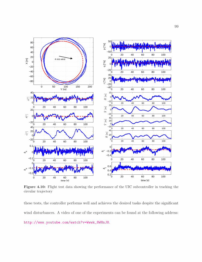
99

0 50 100 150 200

−80

−60

−40

−20

0

20

40

60

80

Y [m]

X [m

]

4 m/s wind

0 20 40 60 80 100−50

0

50

p [°

/s]

0 20 40 60 80 100−20

0

20

q [°

/s]

0 20 40 60 80 100−40−20

02040

r [°

/s]

time [sec]

0 20 40 60 80 100

0

20

40

φ[

]

0 20 40 60 80 100−20

0

20

θ[

]

0 20 40 60 80 100−20

0

20

40

ψ[

]

0 20 40 60 80 100−10

0

10

H[m

]

0 20 40 60 80 100−20

0

20X

[m]

0 20 40 60 80 100−20

02040

Y[m

]

0 20 40 60 80 1000

20

40

R[m

]

0 20 40 60 80 100−0.1

0

0.1

δ e

0 20 40 60 80 100

−0.2

−0.1

0

δ a

time [s]

0 20 40 60 80 100

−0.4

−0.2

0

δ r

0 20 40 60 80 1000.2

0.4

0.6

δ t

time [s]

Figure 4.10: Flight test data showing the performance of the UIC subcontroller in tracking thecircular trajectory

these tests, the controller performs well and achieves the desired tasks despite the significant

wind disturbances. A video of one of the experiments can be found at the following address:

http://www.youtube.com/watch?v=Wwwk_8WHnJ8.

100

Figure 4.11: Flight test results for two switched controllers designed for tracking a Split-S ma-neuver that settles into a circular orbit under relatively high wind conditions; top plots correspondto the case where the planar position error is penalized in the LTV subcontroller design, and bottomplots correspond to the case where the planar position error is not penalized

Chapter 5

Conclusion

In this dissertation, the complete development process of a UAV platform for advanced

control implementation is discussed. The airframe of the platform is obtained from an off-

the-shelf R/C model airplane, the Telemaster, which is modified to incorporate onboard

computers along with several standard and customized sensors. Two airdata probes are

developed, tested, and calibrated to measure the angle of attack, sideslip, and airspeed of

the UAV. Two computers are installed onboard the airplane with each assigned specific

tasks. The resulting architecture enables the implementation of a control algorithm without

interference from such basic functions as sensor data reading, servo actuation, and data

communication.

A mathematical model of the airplane and other substantial subsystems is obtained using

theoretical and empirical tools. Specifically, the output error method is employed to estimate

101

102

the longitudinal and lateral-directional aerodynamic parameters of a postulated model from

flight test data. A second-order model of the servomotors is derived from the frequency

response. In addition, a propulsion model is generated using in part the Javaprop applet.

The dissertation also deals with the optimal control of a small fixed-wing UAV about concate-

nated trajectories. The focus is on trajectory tracking rather than path following. In other

words, the controllers are designed to track dynamically feasible, time-parameterized trajec-

tories. The idea here is that a library of pre-specified motion primitives is designed a priori,

and then the desired trajectories are generated in real-time by concatenating primitives from

this library. A motion planner is typically used to generate the desired trajectories. The

work in this dissertation concerns the design of controllers that would track the desired tra-

jectories despite relatively significant wind disturbances and various other uncertainties. The

approach adopted entails designing subcontrollers corresponding to a subset of the motion

primitives. Then, as the desired trajectory is traversed, the subcontrollers will be applied in

the order of the associated primitives comprising the trajectory. The main contribution of

this work is that it applies systematic LMI-based control tools from robust control theory

to design switched controllers for such a complex system that can track time-parameterized

trajectories despite relatively significant wind disturbances, measurement noise, and other

uncertainties. Specifically, the work demonstrates that recent results on control of systems

with uncertain initial states are especially useful in this case as they can capture the uncer-

tain initial conditions that come about when switching between primitives under disturbances

and other uncertainties. The dissertation provides a rather complete mathematical model of

103

the UAV, based on which the controllers are synthesized, and presents in detail the control

design process. Simulations and flight tests are carried out to demonstrate the performance

of each designed controller.

Bibliography

[1] Austin M. Murch, Yew Chai Paw, Rohit Pandita, Zhefeng Li, and Gary J. Balas. A low

cost small UAV flight research facility. In Florian Holzapfel and Stephan Theil, editors,

Advances in Aerospace Guidance, Navigation and Control, pages 29–40. Springer Berlin

Heidelberg, 2011. 2

[2] T. W. McLain and R. W. Beard. Unmanned air vehicle testbed for cooperative control

experiments. In Proceedings of the American Control Conference, volume 6, pages 5327–

5331, Boston, MA, June-July 2004. 2

[3] D. Jung, E. J. Levy, D. Zhou, R. Fink, J. Moshe, A. Earl, and P. Tsiotras. Design and

development of a low-cost test-bed for undergraduate education in UAVs. In Proceed-

ings of the 44th IEEE Conference on Decision and Control, and the European Control

Conference 2005, pages 2739–2744, Seville, Spain, December 2005. 2, 5

[4] Mark A. Motter, Michael J. Logan, Michael L. French, and Nelson M. Guerreiro. Sim-

ulation to flight test for a UAV controls testbed. In Proceedings of the 25th AIAA

104

105

Aerodynamic Measurement Technology and Ground Testing Conference, San Francisco,

CA, June 2006. 2

[5] T. Jordan, J. Foster, R. Bailey, and C. Belcastro. Airstar: A uav platform for flight

dynamics and control system testing. In (AIAA) 25th Aerodynamic and Measurement

Technology and Ground Testing Conference, June 2006. 2

[6] D. B. Owens, D. E. Cox, and E. A. Morelli. Development of a low-cost sub-scale aircraft

for flight research: The faser project. In (AIAA) Aerodynamic Measurement Technology

and Ground Testing Conference, June 2006. 2, 21

[7] Eloi Pereira, Karl Hedrick, and Raja Sengupta. The C3UV testbed for collaborative

control and information acquisition using UAVs. In Proceedings of the American Control

Conference, pages 1466–1471, Washington, DC, June 2013. 2

[8] R. F. Hartley and F. Hugon. Development and flight testing of a model based autopilot

library for a low cost unmanned aerial systems. In (AIAA) Guidance, Navigation and

Control Conference, August 2013. 2

[9] O. D. Dansker, M. J. Johnson, M. S. Selig, and T. W. Bretl. Development of the

uiuc aero testbed: A large-scale unmanned electric aerobatic aircraft for aerodynamics

research. In (AIAA) Applied Aerodynamics Conference, June 2013. 2

[10] E-Flite. Ultra stick 25e ARF.

URL http://www.e-fliterc.com/Products/Default.aspx?ProdID=EFL4025. 2

106

[11] Carl Goldberg Products Ltd. Goldberg Decathlon ARF.

URL http://www.carlgoldbergproducts.com/decathlonARF.htm. 2

[12] Ardupilot Mega.

URL http://plane.ardupilot.com/. 2, 18

[13] The Paparazzi Project, LLC. Paparazzi.

URL http://paparazzi.enac.fr/. 2

[14] D. W. Bryer and D. E. Walshe. Pressure probes selected for three-dimensional flow

measurement. Repoerts and M 3037, National Advisory Committee for Aeronautics,

1955. 3, 21, 23

[15] R. G. Dominy and H. P. Hodson. An investigation of factors influencing the calibration

of five-hole-probe for three-dimensional flow measurements. Journal of Turbomachinery,

115:513–519, 1993. 3, 23

[16] G. L. Morrison, M. T. Schobeiri, and K. R. Pappu. Five-hole pressure probe analysis

technique. Flow Measurement and Instrumentation, 9:153–158, 1998. 3, 12, 24, 26, 28

[17] Hobby Express International. 6 Foot Telemaster Electro ARF.

URL http://www.hobbyexpress.com/telemasters_216_ctg.htm. 3, 15

[18] Gumstix. Overo Fire COM.

URL https://store.gumstix.com/index.php/products/227/. 3, 18

107

[19] M. Farhood and G. E. Dullerud. Control of nonstationary LPV systems. Automatica,

44(8):2108–2119, August 2008. 4

[20] M. Farhood and G. E. Dullerud. Control of systems with uncertain initial conditions.

IEEE Transactions on Automatic Control, 53(11):2646–2651, December 2008. 4, 8, 64,

69, 87

[21] O. Arifianto and M. H. Farhood. Optimal control of fixed-wing uavs along real-time

trajectories. In 5th Annual DSCC and 11th MOVIC, October 2012. 4, 9

[22] Mazen Farhood. Nonstationary LPV control for trajectory tracking: a double pendulum

example. International Journal of Control, 85(5):545–562, 2012. 4, 67

[23] M. Farhood, Z. Di, and G. E. Dullerud. Distributed control of linear time-varying

systems interconnected over arbitrary graphs. International Journal of Robust and

Nonlinear Control. 4

[24] M. Hepperle. Javaprop - design and analysis of propellers. http://www.mh-

aerotools.de/airfoils/javaprop.htm. 4, 46

[25] M. W. Green. Measurement of the moments of inertia of full scale airplanes. NACA

Technical Note, 1927. 5, 37

[26] M. P. Miller. An accurate method of measuring the moments of inertia of airplanes.

NACA Technical Note, 1930. 5, 37, 38

108

[27] H. A. Soule and M. P. Miller. Experimental determination of the moments of inertia of

airplanes. NACA Technical Report, 1933. 5, 37

[28] R. V. Jategaonkar. Flight Vehicle System Identification: a Time Domain Methodol-

ogy. Progress in Astronautics and Aeronautics. American Institute of Aeronautics and

Astronautics, 2006. 5, 50, 51, 52, 54

[29] N. V. Hoffer, C. Coopmans, A. M. Jensen, and Yang Quan Chen. Small low-cost

unmanned aerial vehicle system identification: A survey and categorization. In Inter-

national Conference on Unmanned Aircraft Systems (ICUAS), pages 897–904, Atlanta,

GA, May 2013. 5

[30] S. A. Salman, A. G. Sreenatha, and J. Y. Choi. Attitude dynamics identification of

unmanned aerial vehicle. International Journal of Control, Automation, and Systems,

4(6):782–787, 2006. 5

[31] M. Manaı, A. Desbiens, and E. Gagnon. Identification of a UAV and design of a

hardware-in-the-loop system for nonlinear control purposes. In Proceedings of the AIAA

Guidance, Navigation, and Control Conference, 2005. 5

[32] E. Frazzoli, M. A. Dahleh, and E. Feron. Maneuver-based motion planning for nonlinear

systems with symmetries. IEEE Transactions on Robotics, 21(6):1077–1091, December

2005. 7

109

[33] C. Goerzen, Z. Kong, and B. Mettler. A survey of motion planning algorithms from the

perspective of autonomous UAV guidance. Journal of Intelligent and Robotic Systems,

57(1-4):65–100, 2009. 7

[34] David J. Grymin, Charles B. Neas, and Mazen Farhood. A hierarchical approach for

primitive-based motion planning and control of autonomous vehicles. Robotics and

Autonomous Systems, 62:214–228, February 2014. 7, 9

[35] Derek R Nelson, D Blake Barber, TimothyWMcLain, and Randal W Beard. Vector field

path following for miniature air vehicles. IEEE Transactions on Robotics, 23(3):519–529,

2007. 7

[36] Isaac Kaminer, Antonio Pascoal, Enric Xargay, Naira Hovakimyan, Chengyu Cao, and

Vladimir Dobrokhodov. Path following for unmanned aerial vehicles using L1 adap-

tive augmentation of commercial autopilots. AIAA Journal of Guidance, Control, and

Dynamics, 33(2):550–564, March 2010. 7

[37] Pascal Gahinet and Pierre Apkarian. A linear matrix inequality approach to h control.

International Journal of Robust and Nonlinear Control, 4:421–448, 1994. 8, 64, 65, 67,

68

[38] G. E. Dullerud and S. G. Lall. A new approach to analysis and synthesis of time-varying

systems. IEEE Transactions on Automatic Control, 44(8):1486–1497, August 1999. 8,

64, 65

110

[39] M. Farhood and G. E. Dullerud. LMI tools for eventually periodic systems. Systems

and Control Letters, 47(5):417–432, December 2002. 8

[40] A. V. Rao, D.A. Benson, C. Darby, M.A. Patterson, C. Francolin, I. Sanders, and G.T.

Huntington. Algorithm 902: GPOPS, a MATLAB software for solving multiple-phase

optimal control problems using the Gauss pseudospectral method. ACM Transactions

on Mathematical Software, 37(2):22:1–39, 2010. 8

[41] V. Gavrilets, E. Frazzoli, B. Mettler, M. Piedmonte, and E. Feron. Aggressive ma-

neuvering of small autonomous helicopters: A human-centered approach. International

Journal of Robotics Research, 20(10):795–807, October 2001. 8, 63

[42] M. W. McConley, M. D. Piedmonte, B. D. Appleby, E. Frazzoli, E. Feron, and M. A.

Dahleh. Hybrid control for aggressive maneuvering of autonomous aerial vehicles. In

19th Digital Avionics Systems Conference, volume 1, 2000. 8

[43] Wei Ren and Randal Beard. Trajectory tracking for unmanned air vehicles with veloc-

ity and heading rate constraints. IEEE Transactions on Control Systems Technology,

12:706–716, 2004. 8, 9

[44] Randal Beard, Derek Kingston, Morgan Quigley, Deryl Snyder, Reed Christiansen, Walt

Johnson, Timothy McLain, and Michael Goodrich. Autonomous vehicle technologies

for small fixed-wing uavs. Journal of Aerospace Computing, Information, and Commu-

nication, 2:92–108, 2005. 8, 9

111

[45] Tamas Keviczky and Gary Balas. Software-enabled receding horizon control for au-

tonomous unmanned aerial vehicle guidance. Journal of Guidance, Control, and Dy-

namics, 29:680–694, 2006. 8, 9

[46] I. Kaminer, A. Pascoal, E. Hallberg, and C. Silvestre. Trajectory tracking forau-

tonomous vehicles: An integrated approach to guidance and control. Journal of Guid-

ance, Control, and Dynamics, 21(1):29–38, jan-feb 1998. 9, 35

[47] W. J. Hough. Autonomous aerobatic flight of a fixed-wing unmanned aerial vehicle.

Master’s thesis, Stellenbosch University, 2007. 9

[48] J. Gillula, H. Huang, M. P. Vitus, and C. J. Tomlin. Design of guaranteed safe maneuvers

using reachable sets: Autonomous quadrotor aerobatics in theory and practice. In 2010

IEEE International Conference on Robotics and Automation, pages 1649–1654, May

2010. 11

[49] R. G. Sanfelice. and E. Frazzoli. A hybrid control framework for robust maneuver-based

motion planning. In 2008 American Control Conference, pages 2254–2259, June 2008.

11

[50] Futaba. S3152. URL http://www.futaba-rc.com/servos/digital.html. 15

[51] Model Motors Ltd. JETI Advance Pro 40.

URL http://www.modelmotors.cz/index.php?page=63. 15

112

[52] Model Motors Ltd. AXI 2826/12.

URL http://www.modelmotors.cz/index.php?page=60&kategorie=2826. 15

[53] Landing Products. APC 13x8E.

URL http://www.apcprop.com/v/downloads/PERFILES_WEB/PER3_13x8E.dat. 15

[54] LORD Corporation. Microstrain 3DM GX3-25.

URL http://www.microstrain.com/inertial/3DM-GX3-25. 15

[55] u-blox AG. Antaris LEA-4T.

URL http://tinyurl.com/Ublox-LEA-4T. 15

[56] Murata Manufacturing Co. Ltd. SCP1000.

URL http://tinyurl.com/vtitechnologyscp1000. 15

[57] Freescale Semiconductor Inc. MPXV7002DP.

URL http://tinyurl.com/freescale-mpxv7002dp. 15

[58] U.S. Standard Atmosphere. U.S. Government Printing Office, Washington, D.C., 1976.

16

[59] Futaba. S617FS.

URL http://www.futaba-rc.com/receivers/air.html. 17

[60] Digi International Inc. XBee-PRO 900.

URL http://tinyurl.com/Digi-Xbee-Pro-900XSC. 17

113

[61] Texas Instruments. OMAP 3530.

URL http://www.ti.com/product/omap3530. 19

[62] Capt. USAF J. E. Zeis. Angle of attack and sideslip estimation using inertial reference

platform. Master’s thesis, Air Force Institute of Technology, 1988. 21

[63] E. Morelli. Real-time aerodynamic parameter estimation without air flow angle mea-

surements. Journal of Aircraft, 49(4):1064–1074, 2012. 21

[64] W. Gracey. Summary of methods of measuring angle of attack. Technical Note 4351,

National Advisory Committee for Aeronautics, 1958. 21

[65] D. Telionis, Y. Yang, and O. Rediniotis. Recent development in multi-hole probe (mhp)

technology. In 20th International Congress of Mechanical Engineering, November 2009.

21

[66] J. W. Naughton, L. N. Cattafesta III, and G. S. Settles. A miniature, fast-response

5-hole probe for supersonic flowfield measurements. In (AIAA) 30th Aerospace Sciences

Meeting & Exhibit, January 1992. 23

[67] A. R. Paul, R. R. Upadhyay, and A. Jain. A novel calibration algorithm for five-hole

pressure probe. International Journal of Engineering, Science and Technology, 3:88–95,

2011. 23

114

[68] B. A. Walther and J. L. Moore. The concept of bias, precision and accuracy, and their

use in testing the performance of species richness estimators, with a literature review

of estimator performance. Ecography, pages 815–829, 2005. 31

[69] J. J. Craig. Introduction to Robotics: Mechanics and Control. Addison-Wesley Longman

Publishing Co., Inc., Boston, MA, USA, 2nd edition, 1989. 35

[70] D. Cabecinhas, C. Silvestre, P. Rosa, and R. Cunha. Path-following control for coordi-

nated turn aircraft maneuvers. In AIAA Guidance, Navigation and Control Conference

and Exhibit, August 2007. 35

[71] M. R. Jardin and E. R. Mueller. Optimized measurements of unmanned-air-vehicle

mass moment of inertia with a bifilar pendulum. Journal of Aircraft, 46:63–75, 2009.

38

[72] T. R. Kane and Gan tai Tseng. Dynamics of the bifilar pendulum. Interantional Journal

of Mechanical Sciences, 9:83–96, 1967. 38

[73] J. E. Williams and S. R. Vukelich. The USAF Stability and Control Digital DATCOM

Volume 1 Users Manual. DTIC-MIL, 1979. 49

[74] Mark Drela. AVL. URL http://web.mit.edu/drela/Public/web/avl/. 49

[75] Tomas Melin. Tornado, URL http://www.redhammer.se/tornado/index.html. 49

[76] J.B. Barlow, W.H. Rae, and A. Pope. Low-speed wind tunnel testing. Aerospace engi-

neering/mechanical engineering. Wiley, 1999. 50

115

[77] V. Klein and E. A. Morelli. Aircraft System Identification: Theory and Practice. Amer-

ican Institute of Aeronautics and Astronautics, 2006. 50, 52

[78] M. B. Tischler and R. K. Remple. Aircraft and Rotorcraft System Identification: En-

gineering Methods with Flight Test Examples. American Institute of Aeronautics and

Astronautics, 2006. 50

[79] R. A. Fisher. On the mathematical foundations of theoretical statistics. Philosoph-

ical Transactions of the Royal Society of London. Series A, Containing Papers of a

Mathematical or Physical Character, 222:pp. 309–368, 1922. 50

[80] J.R. Raol and J. Singh. Flight Mechanics Modeling snd Analysis. CRC Press, 2009. 51

[81] J. A. Mulder, Q. P. Chu, J. K. Sridhar, J. H. Breeman, and M. Laban. Non-linear

aircraft flight path reconstruction review and new advances. Progress in Aerospace

Sciences, 35:673–726, 1999. 52

[82] US Air Force. Flying qualities of piloted airplanes (MILSPEC-F8785 C). http://mil-

spec.tpub.com/MIL-F/MIL-F-8785C/, 1980. 58, 59

[83] J. D. McMinn. Extension of a kolmogorov atmospheric turbulence model for time-based

simulation implementation. Technical report, 1997. 58, 59, 84

[84] N. Bedrossian, S. Bhatt, M. Lammers, L. Nguyen, and Y. Zhang. Zero-prop maneuver

space station demonstration. In 2007 AIAA Guidance, Navigation & Control Confer-

ence, 2007. 63

116

[85] A. Packard. Gain scheduling via linear fractional transformations. Systems and Control

Letters, 22:79–92, 1994. 67

[86] M. Farhood. LPV control of nonstationary systems: a parameter-dependent Lyapunov

approach. IEEE Transactions on Automatic Control, 57(1):209–215, January 2012. 67

[87] J. Lofberg. YALMIP: A toolbox for modeling and optimization in MATLAB. In Pro-

ceedings of the CACSD Conference, Taipei, Taiwan, 2004. Available from http://

control.ee.ethz.ch/~joloef/wiki/pmwiki.php. 80

[88] K. C. Toh, M. J. Todd, and R. H. Tutuncu. SDPT3 — a MATLAB software package

for semidefinite programming. Optimization Methods and Software, 11:545–581, 1999.

80