alpha particles in effective field theory
TRANSCRIPT

1

Universidade de Sao paulo
Master’s Thesis
Alpha Particles in Effective Field Theory
Author:
Cristian Caniu Barros
Supervisor:
Dr. Renato Higa
A thesis submitted in fulfilment of the requirements
for the degree of Master of Science
in the
Grupo de Hadrons e Fısica Teorica
Instituto de Fısica da Universidade de Sao Paulo
December 2014
UNIVERSIDADE DE SAO PAULO
Resumo
Instituto de Fısica da Universidade de Sao Paulo
Mestre em Ciencias
Partıculas Alfa em Teorias de Campo Efetivas
por Cristian Caniu Barros
Nesta tese, nos trabalhamos sobre o problema do sistema de duas partıculas alfa uti-
lizando uma teoria de campos efetiva. O nosso objetivo e abordar os observaveis e a
ressonancia do sistema alfa-alfa de baixa energia identificada como o estado fundamental
do berılio-8. Neste trabalho nos comecamos com uma teoria de campo efetiva em que os
graus de liberdade sao as partıculas alfa interagindo via forcas de contato dependentes
do momento. Estes, em contraste com as forcas que sao dependentes da energia, sao
mais uteis na extensao da teorias para sistemas com mais de duas partıculas alfa. Alem
disso, forcas dependentes do momento nos permitem abordar restricoes causais nos ob-
servaveis, conhecidas como causalidade de Wigner. Nos apresentamos nossos calculos
para o sistema alfa-alfa.

UNIVERSIDADE DE SAO PAULO
Abstract
Instituto de Fısica da Universidade de Sao Paulo
Master of Science
Alpha Particles in Effective Field Theory
by Cristian Caniu Barros
In this thesis we work on the problem of the two-alpha-particle system using a halo/-
cluster effective field theory (EFT). Our goal is to address the alpha-alpha scattering
observables and its low-energy resonance identified as the ground state of Beryllium-8.
In this work we start with an EFT in which the degrees of freedom are the alpha particles
interacting via momentum-dependent contact forces. These, in contrast to forces that
are energy-dependent, are more useful in extending the theory to systems with more
than two alpha particles. Additionally, momentum-dependent forces allow us to address
causal restrictions on scattering observables, known as the Wigner’s causality bound.
We present our EFT calculations for the alpha-alpha system.
Acknowledgements
I would like to thank my advisor R. Higa for guidance throughout this work. I also thank
Profs. M. Robilotta and T. Frederico for participation in the examining committee, with
valuable comments. It was a great pleasure having enlightening conversations with Prof.
U. van Kolck and T. Frederico. I thank my friends, classmates, professors and staff of
the Instituto de Fısica da Universidade de Sao Paulo for contributing to my academic
training. This work was supported initially by the Conselho Nacional de Desenvolvi-
mento Cientıfico e Tecnologico CNPq, (National Council for Scientific and Technological
Development, Brazil) and latter by the Comision Nacional de Investigacion Cientıfica
y Tecnologica CONICYT, (National Commission for Scientific and Technological Re-
search, Chile).
iii
Contents
Abstract i
Abstract ii
Acknowledgements iii
Contents iv
1 Introduction 1
2 Scattering Theory 4
2.1 The general theory of elastic scattering . . . . . . . . . . . . . . . . . . . . 4
2.2 Coulomb scattering . . . . . . . . . . . . . . . . . . . . . . . . . . . . . . . 8
2.3 Two-potential formalism . . . . . . . . . . . . . . . . . . . . . . . . . . . . 10
2.4 Natural length scale and systems with large scattering length . . . . . . . 13
3 Nuclear Effective Theories 15
3.1 Introduction . . . . . . . . . . . . . . . . . . . . . . . . . . . . . . . . . . . 15
3.2 General ideas . . . . . . . . . . . . . . . . . . . . . . . . . . . . . . . . . . 16
3.3 EFT for few-nucleon systems . . . . . . . . . . . . . . . . . . . . . . . . . 17
3.3.1 Systems with scattering length of natural size . . . . . . . . . . . . 21
3.3.2 Systems with large scattering length . . . . . . . . . . . . . . . . . 22
3.3.3 Effective-range corrections . . . . . . . . . . . . . . . . . . . . . . . 23
3.3.4 Coulomb corrections . . . . . . . . . . . . . . . . . . . . . . . . . . 25
4 The Two-alpha-particle System 28
4.1 Introduction . . . . . . . . . . . . . . . . . . . . . . . . . . . . . . . . . . . 28
4.2 EFT with Coulomb interactions . . . . . . . . . . . . . . . . . . . . . . . . 30
4.3 Calculation of the scattering amplitude . . . . . . . . . . . . . . . . . . . 32
4.4 Comparison to data . . . . . . . . . . . . . . . . . . . . . . . . . . . . . . 32
4.5 Analysis of the Wigner bound . . . . . . . . . . . . . . . . . . . . . . . . . 33
5 Conclusions 35
iv

Contents v
A Dimensional regularization 37
B The Coulomb modified scattering amplitude 40
C Divergent integrals and dimensional regularization 43
Bibliography 51

Dedicado a mis padres y familia.
vi

Chapter 1
Introduction
Weakly bound nuclear systems has received enormous attention in the last 20 years.
Numerous reactions involving such systems play central roles in understanding astro-
nomical phenomena such as the creation of interstellar material, supernova explosions,
formation of neutron stars and stellar evolution. In massive stars, it would not be an
exaggeration to say that the most important reaction is the triple-alpha (3α) process
through which carbon (12C) and the heaviest elements in the universe are formed.
The reaction among three alphas always had a rich history of investigative interest.
It is extremely difficult to occur directly due to the Coulomb repulsion. The reaction
rate is significantly increased by the existence of a two-alpha resonance identified as the
ground state of beryllium (8Be). However, this increase is still insufficient to explain the
abundance of carbon in the universe. Addressing this problem, Hoyle [1] suggested the
existence of a genuine three-alpha resonance, through which a beryllium and an alpha
particle would transit before decaying into the ground state of carbon-12. The so-called
Hoyle state was confirmed experimentally three years later [2]. This state, having an
energy very close to the three-alpha threshold, is often cited as strong fact that favors
the anthropic principle [3].
From a theoretical perspective, the Hoyle state remains a challenge. Ab-initio calcula-
tions starting from the interaction between two (NN) and three nucleons (3N) are not
yet capable of reproducing this state without considerable level of approximation. The
main reason is the fact that this state involves very low energies (∼ 0.3 MeV) compared
with the binding energy of the stable ground state of 12C (∼ 7.5 MeV). Variational
calculations [4, 5] or cluster approximation [6] have achieved better agreement with
experimental data.
1
Chapter 1. Introduction 2
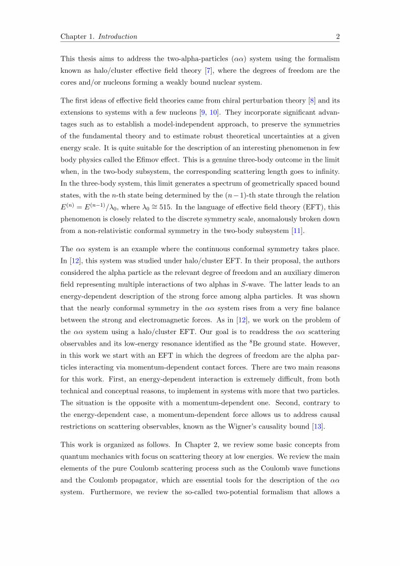
This thesis aims to address the two-alpha-particles (αα) system using the formalism
known as halo/cluster effective field theory [7], where the degrees of freedom are the
cores and/or nucleons forming a weakly bound nuclear system.
The first ideas of effective field theories came from chiral perturbation theory [8] and its
extensions to systems with a few nucleons [9, 10]. They incorporate significant advan-
tages such as to establish a model-independent approach, to preserve the symmetries
of the fundamental theory and to estimate robust theoretical uncertainties at a given
energy scale. It is quite suitable for the description of an interesting phenomenon in few
body physics called the Efimov effect. This is a genuine three-body outcome in the limit
when, in the two-body subsystem, the corresponding scattering length goes to infinity.
In the three-body system, this limit generates a spectrum of geometrically spaced bound
states, with the n-th state being determined by the (n−1)-th state through the relation
E(n) = E(n−1)/λ0, where λ0 ∼= 515. In the language of effective field theory (EFT), this
phenomenon is closely related to the discrete symmetry scale, anomalously broken down
from a non-relativistic conformal symmetry in the two-body subsystem [11].
The αα system is an example where the continuous conformal symmetry takes place.
In [12], this system was studied under halo/cluster EFT. In their proposal, the authors
considered the alpha particle as the relevant degree of freedom and an auxiliary dimeron
field representing multiple interactions of two alphas in S-wave. The latter leads to an
energy-dependent description of the strong force among alpha particles. It was shown
that the nearly conformal symmetry in the αα system rises from a very fine balance
between the strong and electromagnetic forces. As in [12], we work on the problem of
the αα system using a halo/cluster EFT. Our goal is to readdress the αα scattering
observables and its low-energy resonance identified as the 8Be ground state. However,
in this work we start with an EFT in which the degrees of freedom are the alpha par-
ticles interacting via momentum-dependent contact forces. There are two main reasons
for this work. First, an energy-dependent interaction is extremely difficult, from both
technical and conceptual reasons, to implement in systems with more that two particles.
The situation is the opposite with a momentum-dependent one. Second, contrary to
the energy-dependent case, a momentum-dependent force allows us to address causal
restrictions on scattering observables, known as the Wigner’s causality bound [13].
This work is organized as follows. In Chapter 2, we review some basic concepts from
quantum mechanics with focus on scattering theory at low energies. We review the main
elements of the pure Coulomb scattering process such as the Coulomb wave functions
and the Coulomb propagator, which are essential tools for the description of the αα
system. Furthermore, we review the so-called two-potential formalism that allows a
Chapter 1. Introduction 3
simple treatment of the scattering amplitude, with its clean separation into a pure
Coulomb and a Coulomb-modified strong part.
In Chapter 3, we present the main ideas behind effective field theories. In order to
understand the EFT for two alpha particles, we review the EFT for nucleons proposed
by Kaplan et al. [14] and the application to the proton-proton system studied by Kong
and Ravndal [15].
In Chapter 4, we present the strong effective Lagrangian with momentum-dependent
contact interactions and discuss how electromagnetic interactions are included. There is
a subtle difference form Kong and Ravndal’s work due to the presence of a low-energy
S-wave resonance. To renormalize the theory, we compute the αα amplitude to match
the amplitude under the effective-range parametrization. We address the experimental
situation, comparing our predictions to scattering data. Finally, we present our analysis
of the Wigner bound for this specific system.
Our conclusions are outlined in Section 5.

Chapter 2
Scattering Theory
2.1 The general theory of elastic scattering
We begin with a brief overview of scattering theory where the scattered particles, to-
gether with their internal structure, are left unchanged. Emphasis is given to scattering
at relatively small energies which, for nuclear systems, comprises energies of the order
of a few MeVs. The material consulted to prepare this review is well known in the
literature [16–18].
One knowns that a two-body scattering problem is equivalent to the motion of a single
particle, with reduced mass, under the influence of a potential V (r), with r being the
distance between the particles. We consider a short-range central potential V (r) with
r = |r |, to represent the force between two identical particles of mass M . To make
the discussion as simple as possible, we assume the particles spinless, allowing us to
focus on the most important features of the scattering without the complications of a
more realistic description. We carry the analysis in the center-of-mass (c.m.) system.
Throughout this work we adopt a unit system where ~ = c = 1.
We call by ψ the solution of the Schrodinger equation describing the relative motion,
with reduced mass mr = M/2 and positive energy E = p2/2mr, with p the relative
momentum. We require that ψ describes fluxes of incident plus scattered particles, the
latter moving away from the scattering center.
In the presence of a short-range central potential the most general expression for the
wave function reads,
ψ(r) =
∞∑l=0
(2l + 1)Pl(cos θ)ϕl(r), (2.1)
4

Chapter 2. Scattering Theory 5
where ϕl(r) is the solution of the radial Schrodinger equation, and Pl(cos θ) are the
Legendre polynomials (one has m = 0 due to azimuthal symmetry of the problem). The
polar angle θ provides the direction of the scattered particle with respect to the incident
beam. Outside of the range R of the potential, ψ(r) has to match the most general free
solution in terms of spherical Bessel functions, jl(pr) and nl(pr), whose asymptotic form
is known in terms of sine and cosine functions [19].
An usual way to write the asymptotic form of ψ(r) is as follows
ψ(r) ≈ exp(ipz) + f(θ)exp(ipr)
r, (2.2)
where the first term corresponds to the incident beam moving in the z direction with
momentum p, and the second term is the scattered spherical wave modulated by the
so-called scattering amplitude f(θ). The scattering amplitude f(θ) is related to the
differential cross section for elastic scattering within a solid angle element dΩ in the θ
direction through
dσ = |f(θ)|2 dΩ. (2.3)
In order to understand the relation between the Eq. (2.2) and the asymptotic form of
(2.1) it is convenient to compare them with the asymptotic form of the partial-wave
expansion of the free-particle solution,
exp(ipz) ≈∞∑l=0
il(2l + 1)Pl(cos θ)sin(pr − lπ/2)
pr. (2.4)
In the presence of a short-range central potential, the asymptotic expression for ψ can
be expressed in a similar way as Eq. (2.4), the only difference being a phase in the
argument of the sine function in each partial wave,
ψ ≈∞∑l=0
Alil(2l + 1)Pl(cos θ)
sin(pr − lπ/2 + δl)
pr. (2.5)
The coefficient Al must be chosen so that this expression has the form (2.2). Doing so,
one obtains Al = exp(iδl) and the following partial-wave expansion for the scattering
amplitude
f(θ) =∞∑l=0
(2l + 1)Pl(cos θ)
[e2iδl − 1
2ip
]=
∞∑l=0
(2l + 1)Pl(cos θ)
[1
p cot δl − ip
], (2.6)
where δl is known as the partial-wave phase shift. It is a phase in the scattered wave rela-
tive to the free solution, and its dependence with the energy provides useful information
about the interacting potential.

Chapter 2. Scattering Theory 6
At very low energies, in the case where the velocities of the particles under scattering
are so small that their wavelengths are large compared with the typical range R of the
potential (i.e. pR << 1), the phase shift δl(p) approaches zero like p2l+1 [16]. Since p is
small, all the phases δl are small. According to (2.6) in the limit of low energies,
fl ≡1
2ip[exp(2iδl)− 1] ∼ 1
2ip[exp(2ip2l+1)− 1] ∼ p2l. (2.7)
Therefore, the amplitude is dominated by S-wave and can be written as
f(θ) ≈ f0 =e2iδ0 − 1
2ip=
1
p cot δ0(p)− ip. (2.8)
It is worth pointing out that there are some examples where such behavior is not fulfilled.
For instance, f(θ) is dominated by an l 6= 0 component if this channel contains a low-
energy resonance. Another example is two identical fermions in a symmetric spin state,
where the Pauli exclusion principle prevents them to be in S-wave.
At sufficiently low energies the effective-range function Kl
(p2)
[20, 21] is defined by
Kl
(p2)≡ p2l+1 cot δl(p). (2.9)
It is known to be an analytic function of p2 in a large domain of the complex p-plane,
for a large class of potentials. Its expansion in p2 is called the effective-range expansion
(ERE), and for l = 0, it is conventionally expressed in the form
K0
(p2)
= −1
a+
1
2r0p
2 − 1
4P0p4 + ..., (2.10)
where the coefficient a is known as the scattering length, r0 as the effective range, and P0as the shape parameter. The scattering length governs the zero-energy limit p→ 0 and
from Eqs. (2.8) to (2.10) we see that the scattering amplitude is determined uniquely
by a,
f(θ) = −a. (2.11)
By inserting Eq. (2.11) into (2.3) and integrating it, we obtain the total scattering cross
section at zero energy:
σ0 = 4πa2. (2.12)
This is identical to the scattering cross section of an impenetrable sphere of radius a.
It is possible to establish a connection between a and the zero-energy limit of the asymp-
totic form of the wave function, Eq. (2.5). In this limit, the angular dependence of the
wave function ψ is isotropic, since only the l = 0 contribution remains and δ0 ∼ p. Let

Chapter 2. Scattering Theory 7
𝑉(𝑟)
𝑢(0)(𝑟)
𝑟 𝑏
𝑅
𝑤(𝑟)
𝑎
(a) The ground state in a short-range po-tential. The existence of a bound state im-
plies a positive value of a.
𝑉(𝑟)
𝑢(0)(𝑟)
𝑟 𝑅
𝑤(𝑟)
𝑎
(b) When does not exist a bound state, ais taken negative
Figure 2.1: Schematic figure of a ground and unbound state.
us first define the radial function u(p)(r) ≡ rϕ0(r) which satisfies
d2u(p)
dr2−[2mrV (r)− p2
]u(p) = 0 (2.13)
One can easily find a solution to this equation, w(r), valid in the limit p→ 0 and outside
the range R of the potential, w(r) = limp→0 u(p)(r ≥ R). It is satisfies w′′(r) ≈ 0 whose
solution is just a straight line, w(r) = C(r + α) with C and α constants.
On the other hand, the l = 0 term from Eq. (2.5) becomes
limp→0
sin(pr + δ0)
p= lim
p→0
cos δ0(sin pr + cos pr tan δ0)
p= r − a (2.14)
The asymptotic form of u(0)(r) ≈ w(r) = C(r − a) vanishes at r = a. Fig. 2.1 shows
the zero-energy wave function u(0)(r) and w(r) for bound and unbound states. Thus,
the scattering length a can be generally interpreted as the value of r where the function
w(r) becomes zero.
The measurement of the cross section at zero energy determines the absolute value of
the scattering length, but not its sign. Conventionally, the sign of the scattering length
is set by the existence or non-existence of a bound state. When a system has a bound
state at some near zero-energy the radial wave function u(0)(r) decays exponentially with
increasing r in the forbidden zone r > R (the zone at which classically the particles do
not have access) with a decay length b, i.e., u(0)(r) ≈ exp(−r/b). We could say that b is
the size of the ground state and relates to the binding energy B as b = 1/√
2mrB. For
a weakly-bound system b ∼ a. Fig. 2.1 (A) shows the ground state of a bound system.
The existence of a bound sate implies a positive value of a. Conversely, when there is
no bound state, w(r) grows linearly with r, leading to a negative a as shown in Fig. 2.1
(B).
Chapter 2. Scattering Theory 8
In the general theory of scattering, a quantity of interest is the probability amplitude
for a transition from the initial to the final state, the so-called S-matrix:
S(p ′,p) = δ(p ′ − p)− 2πiδ(Ep′ − Ep
)T ≡ 〈p ′|V |ψ(+)
p 〉, (2.15)
where p and p ′ are the initial and final c.m. momenta, respectively. When p2 = p ′2,
with p · p ′ = p2 cos θ the scattering amplitude f(θ) is related to the T -matrix by
f(θ) = −M4πT. (2.16)
2.2 Coulomb scattering
Charged particles, such as alpha particles, interact via electromagnetic forces. In addi-
tion, alpha particles are subjected to the short-range nuclear forces. Throughout this
thesis we take advantage of a formalism that allows a clear separation of pure-Coulomb
and Coulomb-modified nuclear terms. This Section is dedicated to the first part, re-
viewing the main elements of scattering of charged particles interacting only through
the Coulomb potential.
For pure Coulomb scattering it is possible to calculate the differential scattering cross-
section exactly, without the need of relying on the Born approximation or even on the
partial wave expansion. The Schrodinger equation for the Coulomb potential V (r) =
Z1Z2e2/r and a positive energy E = p2/2mr takes the form
− 1
2mr∇2ψ +
Z1Z2e2
rψ =
p2
2mrψ. (2.17)
The solutions can be expressed in terms of an in-state (one that develops out from
a free state in the infinite past) with outgoing spherical waves χ(+)p and an auxiliary
mathematical one (an out-state which develops out backwards in time from a specific
free state in the infinite future) with incoming spherical waves χ(−)p [22]:
χ(+)p (r) = e−
12πηΓ (1 + iη)M (−iη, 1, ipr − ip · r) eip·r , (2.18)
χ(−)p (r) = e−
12πηΓ (1− iη)M (iη, 1,−ipr − ip · r) eip·r , (2.19)
where η is the dimensionless quantity
η =Z1Z2e
2µ
p, (2.20)

Chapter 2. Scattering Theory 9
andM (a, b, z) is the Kummer function (or well-known confluent hypergeometric function
of first kind 1F1(a, b, z)).
Since the Coulomb wave functions 〈r |χ(±)p 〉 = χ
(±)p (r) form a complete set in the repul-
sive case, we can write an useful expression of the Coulomb propagator G(±)C ,
G(±)C (E) ≡ 1
(Ep − H0 − VC ± iε)= 2mr
∫d3q
(2π)3|χ(±)
q 〉〈χ(±)q |
2mrE − q2 ± iε. (2.21)
The Sommerfield factor [16, 23]
C(0)2η ≡
∣∣∣χ(±)p (0)
∣∣∣2 = e−πηΓ(1 + iη)Γ(1− iη) =2πη
e2πη − 1, (2.22)
becomes an important parameter in theories containing Coulomb interactions and rep-
resents the probability density to find the two particles at zero separation.
The asymptotic behavior of the wave function for large r is
χ(+)p (r) ≈ eip·r+iη ln[pr(1−cos θ)] + f(θ)
eipr−iη ln[pr(1−cos θ)]
r, (2.23)
where
f(θ) = −Γ(1 + iη)
Γ(1− iη)
η
p(1− cos θ). (2.24)
The contribution of the logarithmic terms to the phases in Eq. (2.23) makes this wave
function very different from that of Eq. (2.2). The reason arises from the 1/r dependence
of the Coulomb potential. The very slow decrease of this long-range potential influences
the particles even at infinity, leading to a divergent phase proportional to η ln(pr). Real-
istically one knows that the Coulomb potential is shielded at infinity by the existence of
other particles. An appropriate shielding that makes the Coulomb potential vanish be-
yond a very large radius RC is enough to eliminate this divergent phase and restore the
form (2.2) [24]. This is straightforward for two-body systems, but becomes technically
very challenging for systems with three and more particles [25].
Due to the symmetry around the p-direction, the partial-wave expansion of χ(±)p is
independent on the azimuthal angle φ, (i.e. m = 0):
χ(±)p (r) =
∞∑l=0
il(2l + 1)eiσlR±l (pr)Pl(cos θ), (2.25)
where σl is the partial-wave Coulomb phaseshift
σl =1
2iln
Γ(1 + l + iη)
Γ(1 + l − iη)≡ arg Γ(1 + l + iη) (2.26)

Chapter 2. Scattering Theory 10
and R±l (pr) is the solution of the radial Schrodinger equation in the repulsive channel
[16],
R±l (pr) = e−πη/2|Γ(1 + l + iη)|
(2l + 1)!(2pr)leipr 1 F1(1 + l + iη, 2l + 2,−2ipr). (2.27)
The partial-wave form of the amplitude (2.24) can be written in terms of the Coulomb
phase shifts,
f(θ) =
∞∑l=0
(2l + 1)Pl(cos θ)
[e2iσl − 1
2ip
](2.28)
with σl given by (2.26). However, one should keep in mind that this is just a formal
expression, useful to analyze processes within a conserved angular momentum channel.
For observable like cross-sections, that requires the sum over all angular momenta, there
is no guarantee that the sum (2.28) converges. A feel for this may be grasped by looking
at Eq. (2.24) at forward angles, θ ≈ 0. This has a close connection to the fact that
the 1/r Coulomb potential is felt at infinity and therefore, scattering theoretically never
ceases to happen [24].
2.3 Two-potential formalism
The scattering of alpha particles, which are under the combined influence of Coulomb
and nuclear forces, may be simplified by the two-potential formalism [24]. Including the
strong and Coulomb potential via the local operators VS and VC respectively, the system
is described by the wave function |Ψp〉 satisfying
(H0 + VC + VS)|Ψp〉 = Ep|Ψp〉. (2.29)
We now define [26]
|Ψ(±)p 〉 ≡ lim
ε→0
iε
(Ep − H ± iε)|p〉, (2.30)
where H = H0 + VC + VS . The full Green’s function G(±)SC ≡ 1/(Ep − H ± iε) is the
resolvent operator to the Hamiltonian H. Eq. (2.29) is the operation by which stationary
eigenstates of H0, denoted by |p〉, are mapped into specific eigenstates of H.
There are some useful relations between the full, the Coulomb and the free Green’s
functions, where the free operator is G(±)0 ≡ 1/(Ep − H0 ± iε),
G(±)SC = G
(±)0 + G
(±)0 (VC + VS)G
(±)SC (2.31)

Chapter 2. Scattering Theory 11
and
G(±)SC = G
(±)C + G
(±)C VSG
(±)SC . (2.32)
We use (2.31) in (2.30) to separate the full state |Ψ(±)p 〉 into a free and scattered part,
and (2.32) in (2.30) to separate it into a Coulomb and the scattered part,
|Ψ(±)p 〉 =
|p〉+ G
(±)0 (VC + VS)|Ψ(±)
p 〉|χ(±)
p 〉+ G(±)C VS |Ψ(±)
p 〉.(2.33)
Solving in terms of the corresponding asymptotic states we have
|Ψ(±)p 〉 =
[1 + G
(±)SC (VC + VS
)] |p〉 ,[
1 + G(±)SC VS
]|χ(±)
p 〉.(2.34)
From the first line of both Eqs. (2.33) and (2.34), the S-matrix element takes the
standard form
S(p,p ′) = 〈Ψ(−)p |Ψ(+)
p′ 〉 = δ(p − p ′)− 2πiδ(E − E′)〈p|(VC + VS)|Ψ(+)p′ 〉. (2.35)
Where T (p,p ′) ≡ 〈p|(VC + VS)|Ψ(+)p′ 〉 is the total transition amplitude.
Using the following equation
〈p| = 〈χ(−)p | − 〈χ(−)
p |VCG(+)0 (2.36)
and the first line of Eq. (2.33), T (p,p ′) becomes
〈p|(VC + VS)|Ψ(+)p′ 〉 = 〈χ(−)
p |VC |p ′〉+ 〈χ(−)p |VS |Ψ(+)
p′ 〉. (2.37)
At this point we can recognize
TC(p,p ′) ≡ 〈χ(−)p |VC |p ′〉 (2.38)
as the pure Coulomb scattering amplitude and
TSC(p,p ′) ≡ 〈χ(−)p |VS |Ψ(+)
p′ 〉 (2.39)
as the strong scattering amplitude modified by Coulomb corrections.
It will be useful to express the full state in terms of Coulomb states alone,
|Ψ(±)p 〉 =
∞∑n=0
(G(±)C VS)n|χ(±)
p 〉, (2.40)
Chapter 2. Scattering Theory 12
where we used the identity (2.32).
By inserting Eq. (2.40) into (2.39) we have
TSC(p,p ′) =∞∑n=0
〈χ(−)p |VS(G
(+)C VS)n|χ(+)
p′ 〉. (2.41)
The partial wave expansion for TSC is found from Eq. (2.28) and imposing that T (p,p ′)
acquires the phase σl + δl relative to the free solution,
TSC(p,p ′) = −4π
m
∞∑l=0
(2l + 1)e2iσlPl(cos θ)
[e2iδl − 1
2ip
]. (2.42)
In the above expression δl is the phase shift generated by the strong interaction in the
presence of the Coulomb potential.
We end this section with the effective range expansion of TSC . In the presence of the
Coulomb potential, the K-function defined in (2.9) is no longer the analytic function to
be expanded. Instead, the function KSC,l(p2) suitable for the effective-range expansion
is defined as [21, 27, 28]
KSC,l(p2) ≡ p2l+1 C
(l)2η
C(0)2η
[2ηH(η) + C(0)2
η (cot δl − i)], (2.43)
where
C(l)2η =
(l + iη
l
)(l − iηl
)C(0)2η = e−ηπ
(1 + l + iη)(1 + l − iη)
Γ(1 + l)2, (2.44)
and the H-function is related to the digamma function ψ by
H(η) ≡ ψ(iη) +1
2iη− ln(iη). (2.45)
The expansion of this Coulomb-modified effective-range function becomes
KSC,l(p2) = − 1
al+
1
2rlp
2... (2.46)
With this, the S-wave part of the amplitude (2.42) is written as
TSC(p,p ′) = −4π
m
[C2ηe
2iσ0
KSC(p2)− 2kCH(η)
]. (2.47)

Chapter 2. Scattering Theory 13
2.4 Natural length scale and systems with large scattering
length
As shown in Chapter 3, the low and high energy scales of a system are the first ingredients
in the construction of an effective field theory. They provide and expansion parameter
used to identify the operators that are dominant at low energies and to estimate the size
of loop contributions in the calculation of physical observables.
Before going to the main aspects in the construction of an EFT, let us review the
concept of natural length scale ` associated with an interaction potential. This is set by
the typical range R of the potential, i.e. ` ∼ R. For the interacting system, ` sets the
high-momentum scale QH by the de Broglie relation, QH = 1/`. The low-momentum
scale QL is established by the energy of the process.
The effective range expansion can be expressed in terms of the small parameter given
by the ratio between the low- and high-momentum scales, QL/QH << 1,
K(p2)
= −1
a+
1
2Q2H
∞∑n=1
rn
(Q2L
Q2H
)n. (2.48)
For each term to be smaller than the preceding one, the size of the coefficients must be
of the order of the natural length scale, rn ∼ `. If the magnitude |a| of the scattering
length is comparable to `, we say that a has a natural size. In the case |a| >> `, we say
that a is unnaturally large.
Systems having a bound state close to zero energy have a positive scattering length, but
what defines a system with a large scattering length? It is a system where the size b of
the bound state is considerably larger than the range R of the potential, and there is
a considerable probability of finding the two particles in the bound state at a distance
larger than the range of the forces which hold them together. Therefore such bound
state is a rather weakly bound state.
For example, in the spin-singlet channel of the proton-neutron system the scattering
length and the effective range are as ≈ −23.7 fm and rs ≈ 2.7 fm [29]. Moreover, for
nucleon energies much less than the pion mass the effective Lagrangian contains only
contact interactions and the natural length scale of such interactions is established by the
range of the one-pion exchange potential `π = 1/mπ ≈ 1.4 fm (see Chapter 3). Hence,
we see that the effective range is comparable to the natural length scale. However, the
scattering length as is much larger than `π. If as was positive, the bound singlet state of
the system would have a correspondingly large value of R and hence a very low binding
energy, Bs ≈ 100 keV. However, there is no bound singlet state, thus, as is negative.
Chapter 2. Scattering Theory 14
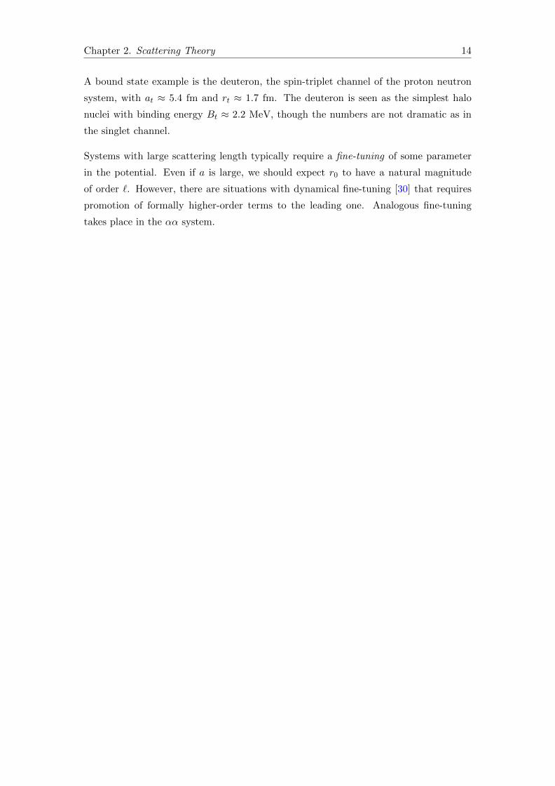
A bound state example is the deuteron, the spin-triplet channel of the proton neutron
system, with at ≈ 5.4 fm and rt ≈ 1.7 fm. The deuteron is seen as the simplest halo
nuclei with binding energy Bt ≈ 2.2 MeV, though the numbers are not dramatic as in
the singlet channel.
Systems with large scattering length typically require a fine-tuning of some parameter
in the potential. Even if a is large, we should expect r0 to have a natural magnitude
of order `. However, there are situations with dynamical fine-tuning [30] that requires
promotion of formally higher-order terms to the leading one. Analogous fine-tuning
takes place in the αα system.

Chapter 3
Nuclear Effective Theories
3.1 Introduction
In chapter 4, we deal with a system of two alpha particles at three-momentum less than
an amount Q of about 20 MeV, the momentum at which the 8Be ground state is reached.
More precisely, we calculate the scattering amplitude of such process using an effective
Lagrangian in which degrees of freedom at energies above those established by pion
exchanges (mπ ≈ 140 MeV) are supposedly integrated out. Such effective Lagrangian
depends only on the relevant alpha field and derivatives thereof.
Because of the low-energy nature of the scattering process considered, effective field
theory is the appropriate theoretical tool to treat it. It provides a framework to calculate
physical observables exploiting the widely separated energy scales of physical systems.
The idea in constructing an effective field theory is not an attempt to reach a theory
of everything, but to construct a theory that is appropriate to the energy scales of the
experiments which we are interested in and take into account only the relevant degrees of
freedom to describe physical phenomena occurring at such energy scales, while ignoring
the substructure and degrees of freedom at higher energies.
The starting point is to identify those parameters which are very large compared with
the energy E of the process of interest. If there is a single mass scale M in a hypo-
thetical underlying theory, the interactions among the light states can be organized as
an expansion in powers of E/M . The underlying idea behind such expansion comes
from a local approximation of non-local operators, the latter being a remnant of inte-
grations of the high-energy degrees of freedom at the Lagrangian level. The information
about the high-energy dynamics is encoded in the couplings of the resulting low-energy
Lagrangian.
15
Chapter 3. Nuclear Effective Theories 16
Although such expansion contains an infinite number of terms, renormalizability is not
a problem because the low-energy theory is specified by a finite number of couplings at
a well-established power in p/Λ. This allows for an order-by-order renormalization.
Based on several reviews and lecture notes existing in the literature [31], in Section 3.2,
we summarize the general ideas in the construction of an effective theory. In Section
3.3, we describe the application to nuclear physics.
3.2 General ideas
Depending on whether or not an underlying theory is known there are two ways to
construct an EFT. When an underlying high-energy theory is known, an effective theory
may be obtained in a top-down approach by a process in which high-energy effects are
systematically eliminated. When an underlying high-energy theory is not known, it may
still be possible to obtain an EFT by a bottom-up approach where relevant symmetries
and naturalness constraints are imposed on candidate Lagrangians.
The top-down approach starts with a known theory and then systematically eliminates
degrees of freedom associated with energies above some characteristic high-energy scale
QH . One method to do that was proposed by Wilson and others in the 1970s [32].
It involves roughly two steps: First, the high-energy degrees of freedom are identified
and integrated out in the action. These high-energy degrees of freedom are referred
to as the high momenta, or heavy, fields. The result of this integration is an effective
action that describes non-local interactions among the low-energy degrees of freedom
(the low momenta, or light, fields). Ultimately, the resulting non-local effective action is
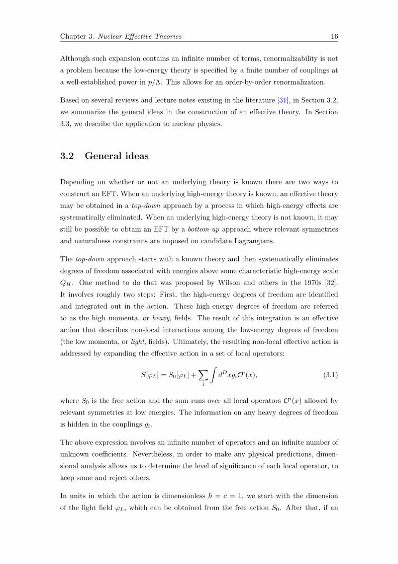
addressed by expanding the effective action in a set of local operators:
S[ϕL] = S0[ϕL] +∑i
∫dDxgiOi(x), (3.1)
where S0 is the free action and the sum runs over all local operators Oi(x) allowed by
relevant symmetries at low energies. The information on any heavy degrees of freedom
is hidden in the couplings gi.
The above expression involves an infinite number of operators and an infinite number of
unknown coefficients. Nevertheless, in order to make any physical predictions, dimen-
sional analysis allows us to determine the level of significance of each local operator, to
keep some and reject others.
In units in which the action is dimensionless ~ = c = 1, we start with the dimension
of the light field ϕL, which can be obtained from the free action S0. After that, if an

Chapter 3. Nuclear Effective Theories 17
operator Oi(x) has been determined to have units ENi , the coupling gi has dimension
D − Ni because dDx has dimension −D and the action must be dimensionless. One
can define dimensionless coupling constants by λi = ΛNi−Dgi. The naturalness property
tells us that these dimensionless couplings should take relative values of order 1 in a
natural theory. This is in contrast with some theories like EFT for few-nucleon systems
at energies below the pion mass [14], where the scattering length is unnaturally large.
The same happens for the EFT of two-alpha system at energies below the pion mass (see
Chapter 4). This will have serious implications in calculations of physical observables.
Dimensional analysis gives for the ith term in (3.1) the following expression to estimate
its size, ∫dDxgiOi(x) ∼
(E
Λ
)Ni−D. (3.2)
Another way to construct an EFT applies when the fundamental high-energy theory
is not known. One simply begins with the operator expansion (3.1), introduces all
operators allowed by low-energy symmetries and introduces couplings which depend
inversely on the high energy scale Λ to the power appropriate for the dimension of
the operator. An example of bottom-up construction is indeed the EFT for the two-
alpha system, the main subject of the present work. A complete discussion about that
is addressed in section four. Another example is, in the view of many physicists, the
Standard Model itself as a low-energy approximation to a more fundamental theory,
such as a unified field theory or string theory.
3.3 EFT for few-nucleon systems
Quantum chromodynamics (QCD) is the theory that deals with the strong interaction
among quarks and gluons [33]. At low-energy scales the confinement property forces
quarks and gluons to remain bound into hadrons such as the proton, the neutron, the
pion or the kaon. Hadrons are the relevant degrees of freedom in the low-energy regime
of QCD. The typical scale of QCD is of the order of 1 GeV, while nucleons in nuclear
matter have typical momentum much smaller than the QCD scale. In the nucleon-
nucleon interaction the low scales are the nucleon momentum p ≈ 280 MeV and the
pion mass mπ ≈ 140 MeV, while the high scales would be the masses of the vector
mesons e.g., mρ ≈ 700 MeV and higher resonances.
The energy gap between the typical scales of QCD and nuclear physics allows the con-
struction of an EFT dealing with the low-energy regime of QCD. This EFT is called
Chiral perturbation theory (ChPT) and is useful to deal with the interaction of hadrons
Chapter 3. Nuclear Effective Theories 18
with pions. It was first suggested by S. Weinberg [8] and systematically developed by
Gasser and Leutwyler [34] (see the review [35]).
The chiral effective Lagrangian consists of a set of operators, ranked based on the num-
ber of powers of the expansion parameters p/Λχ and mπ/Λχ, where Λχ is the chiral
symmetry breaking scale of the order of 1 GeV. These operators are consistent with the
(approximate) chiral symmetry of quantum chromodynamics (QCD) as well as other
symmetries, like parity and charge conjugation.
In nuclear physics, the perturbative aspect of ChPT requires changes due to the non-
perturbative aspects of nuclear processes. This so-called chiral EFT was proposed by
Weinberg [9] and carried out by van Kolck and others [36]
However, in Weinberg’s original work the power counting scheme proposal was shown
not to be consistent, encountering difficulties coming from the large scattering length in
the 1S0 and 3S1 NN scattering amplitudes. These difficulties were outlined by Kaplan,
Savage and Wise [14, 37], where they developed a technique, which we present here, for
computing properties of nucleon-nucleon interactions. Similar to this technique is the
approach that we want to use to describe the two-alpha system.
For energies much less than the pion mass the only relevant degree of freedom is the
non-relativistic nucleon field N of mass M and the appropriate expansion parameter
is p/Λ, where Λ is set by the pion mass (Λ ∼ mπ). The effective Lagrangian for non-
relativistic nucleons must obey the symmetries of the strong interactions at low energies,
i.e. parity, time-reversal and Galilean invariance. It only contains contact interactions,
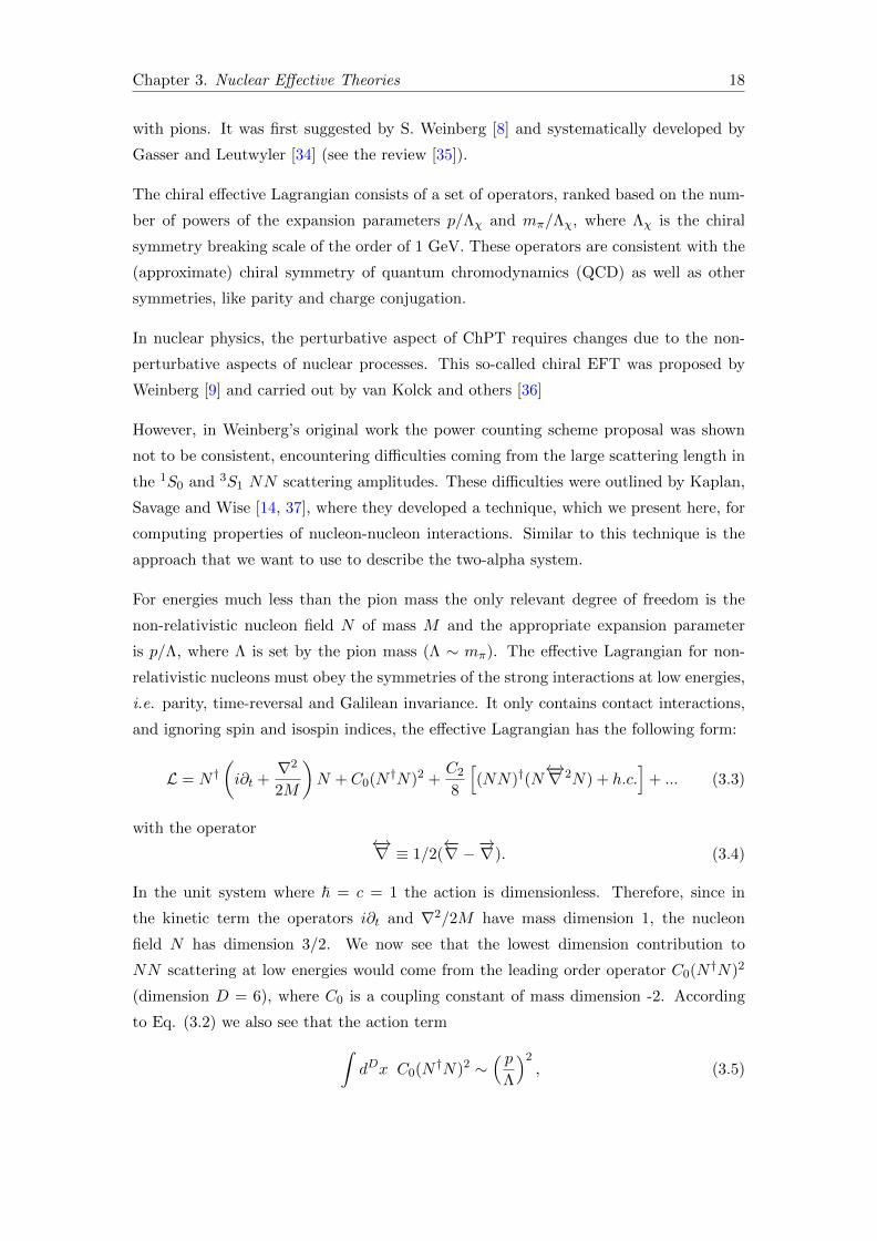
and ignoring spin and isospin indices, the effective Lagrangian has the following form:
L = N †(i∂t +
∇2
2M
)N + C0(N
†N)2 +C2
8
[(NN)†(N
←→∇ 2N) + h.c.
]+ ... (3.3)
with the operator←→∇ ≡ 1/2(
←−∇ −
−→∇). (3.4)
In the unit system where ~ = c = 1 the action is dimensionless. Therefore, since in
the kinetic term the operators i∂t and ∇2/2M have mass dimension 1, the nucleon
field N has dimension 3/2. We now see that the lowest dimension contribution to
NN scattering at low energies would come from the leading order operator C0(N†N)2
(dimension D = 6), where C0 is a coupling constant of mass dimension -2. According
to Eq. (3.2) we also see that the action term∫dDx C0(N
†N)2 ∼( p
Λ
)2, (3.5)

Chapter 3. Nuclear Effective Theories 19
Figure 3.1: Four-nucleon vertex.
while the second term: ∫dDx C2(NN)†(N
←→∇ 2N) ∼
( pΛ
)4. (3.6)
From these equations we see that at low energies the first one dominates, so that in the
limit where the energy goes to zero, the interaction of the lowest dimension remains and
one can use the following effective Lagrangian,
L = N †(i∂t +
∇2
2M
)N + C0(N
†N)2. (3.7)
The C0 interaction in (3.7) is non-renormalizable and correspond to a singular delta
function potential. It is represented by the four nucleon vertex in Fig. 3.1.
From quantum mechanics in the limit where the energy goes to zero, due to the effective
range expansion, Eq. (2.10), the S-wave partial wave amplitude depends on a single
parameter, the scattering length a,
T (p) = −4π
M
1
p cot δ(p)− ip= −4π
M
1
−1/a− ip, (3.8)
where p is the relative momentum.
In quantum field theory, the amplitude T is given by the sum of Feynman diagrams. It
is the sum of the four nucleon vertex, the bubble diagram in Fig. 3.2 and the multi-loop
Feynman diagrams in Fig. 3.3. The rules to computing them are simple: For each vertex
we have
V = iC0, (3.9)
while the nucleon propagator is
i∆(q) =i
q0 − q2/2M + iε. (3.10)
For each bubble we need to incorporate the loop integral
I =
∫d4q
(2π)4· i
E/2− q0 − q2/2M + iε· i
E/2 + q0 − q2/2M + iε, (3.11)
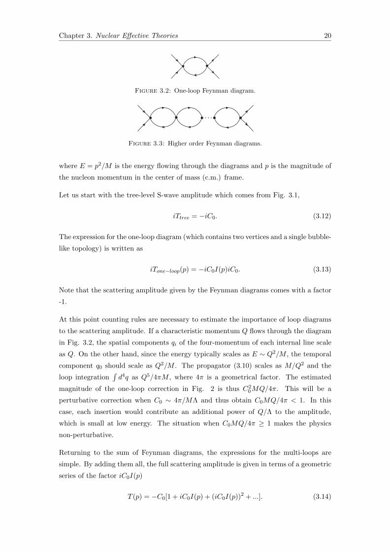
Chapter 3. Nuclear Effective Theories 20
Figure 3.2: One-loop Feynman diagram.
Figure 3.3: Higher order Feynman diagrams.
where E = p2/M is the energy flowing through the diagrams and p is the magnitude of
the nucleon momentum in the center of mass (c.m.) frame.
Let us start with the tree-level S-wave amplitude which comes from Fig. 3.1,
iTtree = −iC0. (3.12)
The expression for the one-loop diagram (which contains two vertices and a single bubble-
like topology) is written as
iTone−loop(p) = −iC0I(p)iC0. (3.13)
Note that the scattering amplitude given by the Feynman diagrams comes with a factor
-1.
At this point counting rules are necessary to estimate the importance of loop diagrams
to the scattering amplitude. If a characteristic momentum Q flows through the diagram
in Fig. 3.2, the spatial components qi of the four-momentum of each internal line scale
as Q. On the other hand, since the energy typically scales as E ∼ Q2/M , the temporal
component q0 should scale as Q2/M . The propagator (3.10) scales as M/Q2 and the
loop integration∫d4q as Q5/4πM , where 4π is a geometrical factor. The estimated
magnitude of the one-loop correction in Fig. 2 is thus C20MQ/4π. This will be a
perturbative correction when C0 ∼ 4π/MΛ and thus obtain C0MQ/4π < 1. In this
case, each insertion would contribute an additional power of Q/Λ to the amplitude,
which is small at low energy. The situation when C0MQ/4π ≥ 1 makes the physics
non-perturbative.
Returning to the sum of Feynman diagrams, the expressions for the multi-loops are
simple. By adding them all, the full scattering amplitude is given in terms of a geometric
series of the factor iC0I(p)
T (p) = −C0[1 + iC0I(p) + (iC0I(p))2 + ...]. (3.14)

Chapter 3. Nuclear Effective Theories 21
From Eq. (3.8) we see that the radius of convergence of a momentum expansion of
T (p) depends on the size of the scattering length a. For example, when the scattering
length has a natural size, |a| ∼ 1/Λ, the expansion parameter ap << 1 allows writing
the expression for the scattering amplitude Eq. (3.8) in the form
T (p) =4πa
M[1− iap+ (iap)2 − (iap)3 + ...], (3.15)
Reproducing it in EFT depends on the size of the coupling constant and on the subtrac-
tion scheme used to render all the diagrams finite.
3.3.1 Systems with scattering length of natural size
For the perturbative situation a ∼ 1/Λ, the scenario is simple. In order to reproduce the
momentum expansion Eq. (3.15), one can use the minimal subtraction (MS) scheme,
the appropriate scheme to absorb the infinities that arise in perturbative calculations
beyond leading order [38, 39]. Using dimensional regularization, one has for the one-loop
integral in Eq. (3.11) the following expression (see Appendix A)
I(p) = −iM(−ME − iε)(D−3)/2Γ(
3−D2
)(µ/2)4−D
(4π)(D−1)/2, (3.16)
where µ is the renormalization mass and D is the dimensionality of the space-time. The
MS scheme amounts to subtracting any 1/(D − 4) pole before taking the D → 4 limit.
The integral Eq. (3.16) does not exhibit any such poles and so the result is simply
IMS(p) =
(M
4π
)p (3.17)
Since there are no poles at D = 4 in the MS scheme the coefficient C0 is independent on
the renormalization scale µ. Comparing Eqs. (3.14) and (3.15) we find for the coupling
of the effective theory
C0 = −4πa
M. (3.18)
In this scheme C0I(p) ∼ p/Λ and the effective field theory is thus completely perturba-
tive. The perturbative sum of Feynman graphs thus corresponds to a Taylor expansion
of the scattering amplitude.
The MS scheme is appropriate for a perturbative renormalization, it is the case when
the scattering length has a natural size. However, when this is unnaturally large, a
non-perturbative renormalization is required. This situation is discussed in the next
section.
Chapter 3. Nuclear Effective Theories 22
3.3.2 Systems with large scattering length
Previously in Section 2.4 we have already mentioned systems with large scattering length.
The proton-neutron system is the best known example with this condition. In the 1S0
channel the scattering length as ≈ −23.7 fm is much larger than the natural length scale
of the system, `π ≈ 1.4 fm.
For these kind of systems, due to the large value of the scattering length, in the limit of
zero energy, the absolute value |ap| is no longer the expansion parameter. Consequently,
the scattering amplitude Eq. (3.8) can no longer be written as a perturbative Taylor
series. Instead, this corresponds to a non-perturbative situation, where the Feynman
diagrams must be considered to all orders in the loop expansion. The fact that Eq.
(3.14) forms a geometric series allows one to perform the sum, leading to
T (p) = − C0
1− iC0I(p). (3.19)
Regarding renormalization, the large value of the scattering length turns the situation
non-perturbative forcing one to look for a non-perturbative renormalization. It was
shown in [40] that, in a non-perturbative situation, the MS scheme in dimensional reg-
ularization fails to reproduce the correct functional form of the scattering amplitude.
The reason for this failure is known—contrary to perturbative renormalization, in the
non-perturbative regime power divergences from loop integrals are crucial in driving the
renormalization flow of the coupling constants. The usual dimensional regularization
ignores all but the log-divergences [40].
A consistent non-perturbative renormalization was introduced by Kaplan, Savage and
Wise [37], the so-called power-divergences subtraction (PDS) scheme. This involves
subtracting from the dimensionally regulated loop integral not only the 1/(D−4) poles,
but also poles in lower dimensions. This would make possible to recover the desired µ
scale from the loop integral. To see that, let us apply it to the regulated integral (3.16).
It has no pole at D = 4, but it does have a pole at D = 3, coming from the gamma
function. This pole is related to the ultraviolet linear divergence present in the loop
integration. So, in the D → 3 limit we have the pole
δI = −i Mµ
4π(3−D), (3.20)
and then the subtracted integral, back to the D → 4 limit, is
IPDS(p) =M
4π(p− iµ). (3.21)

Chapter 3. Nuclear Effective Theories 23
In this way, we have recovered the µ-dependence from the loop integrals. Putting this
into the Eq. (3.19) we have
T (p) = − 1
1/C0 − i(M/4π)(p− iµ). (3.22)
The above amplitude must be independent of the arbitrary parameter µ. This require-
ment strongly affects the values of the coupling constant whose dependence on µ is
determined by the renormalization group equations, where the physical parameter a
enters as a boundary condition.
In this case, we can obtain the µ-dependence of C0 simply by comparing the amplitudes
(3.22) and (3.8),
C0(µ) =4π
M
(1
µ− 1/a
). (3.23)
When only the lowest order C0 interaction is included in the effective Lagrangian we see
that there is no contribution to the effective range r0. One should be able to include
corrections to the scattering amplitude by including higher order interactions in the
effective theory, therefore improving the accuracy of the calculation.
3.3.3 Effective-range corrections
From quantum mechanics, the low-energy scattering amplitude is parametrized in terms
of the scattering length a and the effective range r0. Treating the latter as a small
correction, the amplitude has the following momentum expansion
T (p) = −4π
M
1
−1/a+ r0p2/2− ip= −4π
M
1
−1/a− ip
[1− r0/2
−1/a− ipp2 +O(p4/Λ4)
].
(3.24)
The goal in this case is to show how a similar correction is obtained from EFT.
We saw that the leading C0 term has dimension D = 6 and dominates in the limit where
the energy goes to zero. Its contribution to the amplitude scales as p−1 and correspond
to the expression (3.22). According to (3.2) the next to leading order operator
L2 =C2
8(NN)†(N
←→∇ 2N) + h.c., (3.25)
has dimension D = 8 and, for a natural behavior of the C2 coupling, must be treated
in first order of perturbation theory. This is equivalent to assume a natural size for the
effective range, r0 ∼ 1/Λ. Its contribution is given by the sum of Feynman diagrams
shown in Figure 3.4. Feynman rules give for the C2 interaction the corresponding vertex
Chapter 3. Nuclear Effective Theories 24
(a)
(b)
(c)
(d)
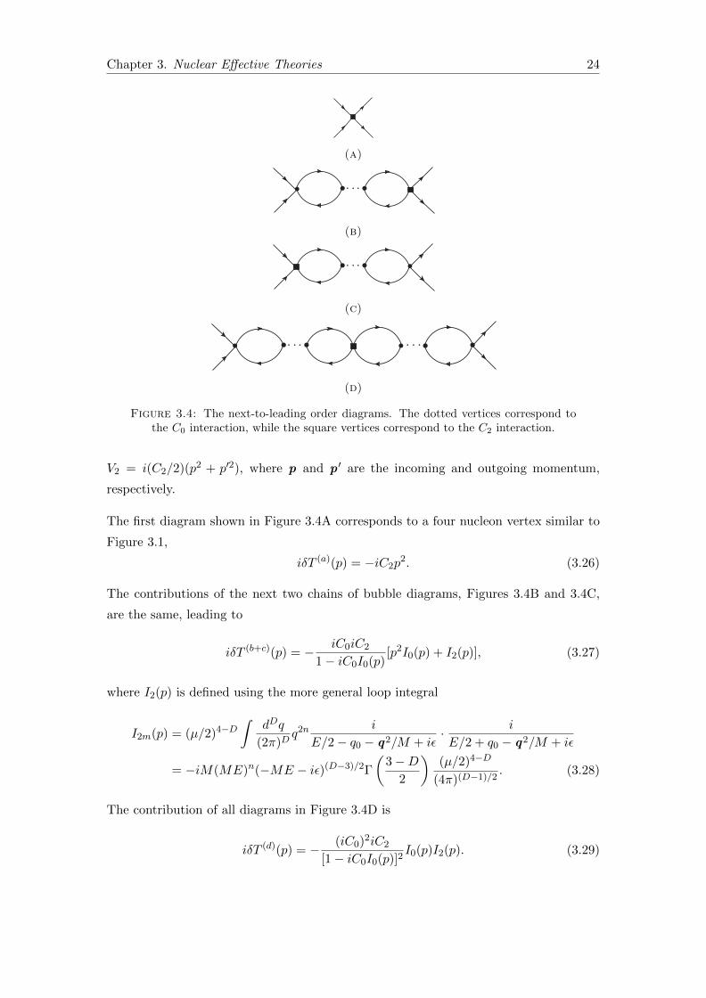
Figure 3.4: The next-to-leading order diagrams. The dotted vertices correspond tothe C0 interaction, while the square vertices correspond to the C2 interaction.
V2 = i(C2/2)(p2 + p′2), where p and p ′ are the incoming and outgoing momentum,
respectively.
The first diagram shown in Figure 3.4A corresponds to a four nucleon vertex similar to
Figure 3.1,
iδT (a)(p) = −iC2p2. (3.26)
The contributions of the next two chains of bubble diagrams, Figures 3.4B and 3.4C,
are the same, leading to
iδT (b+c)(p) = − iC0iC2
1− iC0I0(p)[p2I0(p) + I2(p)], (3.27)
where I2(p) is defined using the more general loop integral
I2m(p) = (µ/2)4−D∫
dDq
(2π)Dq2n
i
E/2− q0 − q2/M + iε· i
E/2 + q0 − q2/M + iε
= −iM(ME)n(−ME − iε)(D−3)/2Γ(
3−D2
)(µ/2)4−D
(4π)(D−1)/2. (3.28)
The contribution of all diagrams in Figure 3.4D is
iδT (d)(p) = − (iC0)2iC2
[1− iC0I0(p)]2I0(p)I2(p). (3.29)
Chapter 3. Nuclear Effective Theories 25
The sub-leading contribution to the scattering amplitude comes from the sum of these
three partial results,
δT (p) = − C2
[1− iC0I0(p)]2[p2 − iC0(p
2I0(p)− I2(p))]. (3.30)
To assure a correct renormalization the divergent integrals I0 and I2 must be regularized
within the PDS scheme. After that, I0 corresponds to Eq. (3.21) and the new divergent
integral I2 becomes
I2(p) = p2M
4π(p− iµ). (3.31)
Therefore, using PDS, the factor (p2I0− I2) in the numerator of (3.30) vanishes and the
sub-leading contribution becomes
δT (p) = − C2p2
[1− i(C0M/4π)(p− iµ)]2. (3.32)
Once again δT is independent of the renormalization mass µ and the µ-dependence of
the couplings is determined by this fact. We now expect that the leading and sub-leading
contributions to the scattering amplitude, Eqs. (3.22) and (3.32) respectively, allow us
to reproduce the expansion (3.25). Putting them together we have
T (p) = T0
[1 +
δT
T0
]= −4π
M
1
(4π/MC0)− µ− ip
[1 +
C2p2
C0[1 + (MC0/4π)(µ+ ip)]
].
(3.33)
Comparing it with the expansion (3.25) we obtain for C0 basically the same expres-
sion (3.23), whereas for the new coupling constant C2, the µ-dependence comes with a
dependence on the effective range r0,
C2(µ) =4π
M
(1
µ− 1/a
)2 r02. (3.34)
3.3.4 Coulomb corrections
In the previous section we saw the corrections to the amplitude (3.22) that arise when
considering the higher order C2 interaction in first order of perturbation theory. Now, we
want to show how to include electromagnetic interactions for cases where the scattered
particles are charged. We follow the analysis made by Kong and Ravndal [15] for the
proton-proton system.

Chapter 3. Nuclear Effective Theories 26
Figure 3.5: Lowest order Coulomb correction to the four-nucleon vertex.
Electromagnetic interactions are included by minimal substitution, ∂µ → ∂µ + ieAµ,
where Aµ is the electromagnetic four-potential and e is the electric charge. An appro-
priate gauge choice is essential for a straightforward treatment. We choose the Coulomb
gauge, defined by the gauge condition ∇ · A(r , t) = 0, in order to allow a separation
between Coulomb and transverse radiative photons. We start from the effective La-
grangian (3.7), in this section renamed to L0. Changing the derivatives according to the
minimal substitution and adding the electromagnetic Lagrangian Lγ0 (see Ref. [41] for
scalar electrodynamics) yield
L = L0(N) + Lγ0(A) + Lint, (3.35)
where
Lint = −eA0(N†N) + i
e
MN †(A · ∇N)− e2
2MA2(N †N). (3.36)
The first term of Lint corresponds to the interaction among nucleons and Coulomb
photons coupling through the electric charge. The second and third terms correspond
to the interaction among nucleons and transverse photons coupling additionally through
the proton velocity and the electric charge respectively. In comparison to the Coulomb
photons, the effects of the transverse photons are negligible in both NN [15] and αα
[12] scattering.
As result, Kong and Ravndal found that each photon exchange is proportional to the
Sommerfeld parameter η = kC/p, where kC is Coulomb scale. For instance, the Coulomb
correction for the four-nucleon vertex shown in Fig. 3.1 is given by the Feynman diagram
in Fig. 3.5. Counting rules give for this term
δT (p) = C0
∫d3q
(2π)3e2
q2 + λ2M
p2 − (p − q)2 + iε∼ C0
kCp
(3.37)
where λ → 0 is the photon mass which acts as an infrared regulator. For one more
Coulomb photon exchange in the four-nucleon vertex, counting rules give a contribution
of the order C0η2. Thus, for momentum p ≤ kC the Sommerfeld parameter η = kC/p ≥
1, and the Coulomb repulsion must be included in a non-perturbative way.
In non-perturbative cases, the Coulomb propagator (2.21) results from the infinite sum
Chapter 3. Nuclear Effective Theories 27
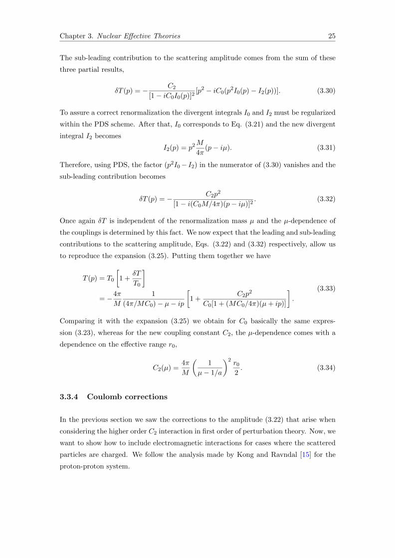
Figure 3.6: Coulomb propagator as a infinite sum of Coulomb photon exchanges [15].
(a)
(b)
(c)
Figure 3.7: Coulomb-distorted Feynman diagrams. The shaded bubble represents ainfinite sum of non-perturbative Coulomb contributions.
of Feynman diagrams shown in Figure 3.6, with zero, one, two, etc., photon exchanges
[15]. Such diagrams result from the iteration of the integral equation
G(±)C = G
(±)0 + G
(±)0 VCG
(±)C
= G(±)0 + G
(±)0 VCG
(±)0 + G
(±)0 VCG
(±)0 + ... (3.38)
On the other hand, the two potential formalism gives for TSC the expression (2.41),
which can be expressed as the diagrammatic form shown in Figure 3.7, where the shaded
bubbles represents the same infinite sum of non-perturbative Coulomb contributions of
Figure 3.6. In the αα system the Sommerfeld parameter is large, therefore, the Coulomb
repulsion must be included in a non-perturbative way.

Chapter 4
The Two-alpha-particle System
4.1 Introduction
The alpha particle, the nucleus of the helium (4He) atom, is made out of two protons
and two neutrons. Its ground state has a zero total angular momentum Jπ = 0+, and
it can be a positive-parity mixture of three 1S0, six 3P0 and five 5D0 orthogonal states
[42]. It must be clear that, at low energies, the S-wave is the dominant part of the
wave function, with a small D-wave and almost negligible P -wave contributions. Then
at low energies, the alpha particle is essentially in S-wave and its space wave function is
symmetric under the interchange of either two protons, or two neutrons. In the ground
state, the constituents of the alpha particle are strongly bound as shown in Figure 4.1.
It shows the average binding energy per nucleon of common isotopes, where for the 4He
the energy is relatively high.
à
à
à
à
à
à
à
à
à
à
à
à
àà à
à
à à à àà
à àààà à
àà
à àà à à
àà
2H
16O12C
4He
235U206Pb
182W150Nd136Xe
127I116Sn
98Mo75As56Fe35Cl27Al19F
14N9Be
11Be7Li
6Li
3H
176Hf144Nd
130Xe124Xe107Ag
86Sr63Cu40Ar31P20Ne
238U210Po
194Pt
0 50 100 150 2000
2
4
6
8
10
Number of nucleons in nucleus, A
Ave
rage
bind
ing
ener
gype
rnu
cleo
nHM
eVL
Figure 4.1: The average binding energy per nucleon of common isotopes [43].
28

Chapter 4. The Two-alpha-particle System 29
Figure 4.2: Energy levels of 4He are plotted on a vertical scale giving the c.m. energy,in MeV, relative to its ground state. Horizontal lines representing the levels are labeledby the level energies and values of total angular momentum, parity, and isospin (Jπ, I)
[44].
In addition to the ground sate, Figure 4.2 shows the excited states of the 4He. The first
three I = 0 states, 0+, 0− and 2−, are observed to have energies above 20 MeV in the
center of mass frame relative to its ground state.
The present amount of 4He in the universe is mostly attributed to the Big Bang nu-
cleosynthesis, the process by which the first nuclei were formed about three minutes
after the Big Bang. It was then created the hydrogen and helium to be the content of
the first stars. With the formation of the stars, the creation of 4He continues to day
through hydrogen fusion. Also in stars, other heavier nuclei are formed from preexisting
hydrogen and helium nuclei. Besides nucleosynthesis alpha particles may emerge from
alpha decay [20] of heavy radioactive nuclei. This decay is favorable for nuclei of mass
number A above 191.
The strong binding of alpha particles and the fact that they may emerge from a heavy
nucleus led some investigators to conjecture that alpha particles also exist as stable
substructures inside these heavy nuclei before they decay. They suggested that the
binding energies of some Z = N (that is, equal number of protons and neutrons), with
Z even, may be described by a simple model with an integer number of alpha particles.
Although this is generally disputed (alpha particles can not maintain their identity for a
very long time inside condensed nuclear matter), Wheeler [45] and others spoke in terms
of relative average lifetimes at which alpha particles maintain their identities, at least
as far as the low excited states of the nucleus are concerned.
In a modern approach, EFT has been used within the same spirit. It has been used
to deal with halo nuclear states [46, 47]: a nucleus consisting of a tightly bound core

Chapter 4. The Two-alpha-particle System 30
and one or more weakly bound (valence) nucleons. In a first approximation, the core
is treated as an explicit degree of freedom and the EFT is written in terms of contact
interactions between the valence nucleons and the core. Other effects like the size and
shape of the core are encapsulated in a derivative expansion of local operators. Systems
like the 7Be core with a weakly bound proton is considered a halo nuclear state forming
the 8B nucleus [48].
As in the past, alpha particles have been received special attention. In halo nuclear
states, like neutron-alpha (nα) and proton-alpha (pα) systems, alpha particles are con-
sidered as a core whenever the energy of the valence nucleons is smaller compared with
the excitation energy of the alpha particles. The nuclear interaction between nucleons
and alpha particles have been studied separately in neutron-alpha [30, 49] and proton-
alpha [50] scattering, while the αα interaction has been studied by Higa, Hammer, and
van Kolck [12]. These interactions are important input to systems with more than two
alpha particles in multi-body calculations, like the triple-alpha (3α) reaction describing
the formation of 12C via the Hoyle state.
As in [12], we work on the problem of the αα system readdressing the scattering observ-
ables and its low-energy resonance identified as the 8Be ground state. This, is a (0+, 0)
state and has a c.m. energy ER ≈ 0.1 MeV above the αα threshold (the threshold for
break-up into two alpha particles), with a narrow decay width of Γ ≈ 6 eV.
In Section 4.2, we present the strong effective Lagrangian with momentum-dependent
contact interactions and discuss how electromagnetic interactions are included. In Sec-
tion 4.3, we compute the αα amplitude to match the amplitude under the effective-range
parametrization. The experimental situation is discussed in Section 4.4. Finally, the
analysis of the Wigner bound is addressed in Section 4.5.
4.2 EFT with Coulomb interactions
The energy of the 8Be ground state ER = 0.1 MeV is determined from alpha-alpha scat-
tering across the resonance region, and is much smaller than the alpha-particle excitation
energy Ex ≈ 20 MeV. Thus, an EFT may be constructed to calculate observables at
momentum around the resonance region. The low-momentum scale is set by the energy
of such process, QL ∼ kR =√mαER ≈ 20 MeV, where we used the mass of the 4He,
mα ≈ 3.7 GeV, while the breakdown momentum scaleQH is established by the first inter-
nal degrees of freedom that appear within the alpha particle. These include nucleons at
momentum√mNEx ≈ 140 MeV, and pions at momentum of the order of the pion mass

Chapter 4. The Two-alpha-particle System 31
mπ ≈ 140 MeV. Thus, an estimation is that this scale is QH ∼√mNEx ∼ mπ ≈ 140
MeV.
At energies below the pion mass, each alpha particle may be represented by a scalar-
isoscalar field Φ. As before, other effects like nucleus deformation are encapsulated in a
derivative expansion. This EFT provides a controlled expansion of observables, where
the small parameter is given by the ratio between the low- and high-momentum scales
QL/QH ∼ 1/7.
Far below the alpha excitation level, the interactions between two alphas are only in
the S-wave channel. Thus, the proposed EFT for alpha particles interacting through
contact interactions has the following strong effective Lagrangian:
L = Φ†(i∂t +
∇2
2mα
)Φ + C0
(Φ†Φ
)2+C2
8
[(ΦΦ)†
(Φ(←→∇)2
Φ
)+ h.c.
]+ ..., (4.1)
where C0 and C2 are coupling constants. The ellipsis represent higher derivative opera-
tors.
The difference from Kong and Ravndal’s work [15] is due to the existence of the low-
energy resonance in the αα system. To observe that, the two coupling constants must be
considered in leading order [12]. This is different from [15], where the authors considered
C0 as leading order and C2 in first order of perturbation theory.
As in Chapter 3, the Coulomb repulsion comes in a non-perturbative way. The charge of
each alpha particle is Zα = 2 and the reduced mass is mr = mα/2, with mα = 3.7 GeV.
The Coulomb momentum scale is kC = Z2ααemmr ≈ 60 MeV. At momentum k smaller
than kC the Sommerfeld parameter η = kC/k > 1 and the Coulomb repulsion must
be included in a non-perturbative manner. After minimal substitution, the Coulomb
gauge choice allows to separate the Coulomb and transverse photons. Neglecting the
higher-order effects of the latter [12, 15], only the Coulomb repulsion plus the strong
interaction appear in the equations of the two-potential formalism developed in Section
2.3. Accordingly, the T -matrix element can be written as the sum of two parts
T = TC + TSC , (4.2)
where TC and TSC are the pure-Coulomb and Coulomb-modified strong scattering am-
plitude, respectively.

Chapter 4. The Two-alpha-particle System 32
4.3 Calculation of the scattering amplitude
Here, we present the amplitude TSC derived from our EFT leaving the details in the
Appendices B and C. The resulting TSC has the same form as the parametrized formula
(2.47). The corresponding expression for the KSC(p2) is
KSC(p2) = − 4π
mα
(1 + C22 I3)
2[C0 − 2C2(k2C + kCµ)−
(C22
)2I5
]+[C2 +
(C22
)2I3
]p2− I1
,(4.3)
where µ is the renormalization scale and I1, I3 and I5 are divergent integrals (labeled
by its degree of divergence) defined by the general expression,
In = mα
∫d3q
(2π)32πηq
e2πηq − 1qn−3. (4.4)
In order to do a consistent matching with the effective-range parameters (and thus a
correct renormalization of the theory), the right side of (4.3) must be expanded. The
only way to do that seems to be exploiting the I3 and I5 divergences. Since I5 is more
divergent than I3, it is possible the construction of an expansion parameter. However,
to do that, we need to evaluate the scale µ at infinity, in the regularized expressions
for I3 and I5, Eqs. (C.46) and (C.51) respectively. Assuming that this is possible, we
obtain the renormalization conditions
mα
4πa0=
(1 + C22 I3)
2[C0 − 2C2(k2C + kCµ)−
(C22
)2I5
] − I1, (4.5)
mαr08π
=(mα
4πa+ I1
)2( 1
I3− 1
I3(1 + C2I3/2)2
). (4.6)
These equations close the calculation of the αα amplitude. The Coulomb-modified
effective-range parameters fix our EFT parameters and allows our comparison with the
experimental data.
4.4 Comparison to data
In this Section we address the experimental situation regarding the scattering of alpha
particles at low energies and we present the theoretical phase shift derived from the
theory.
Chapter 4. The Two-alpha-particle System 33
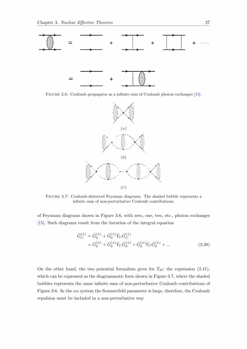
a0 (103 fm) r0 (fm) P0 (fm3)
LO −1.8 1.083 -NLO −1.92± 0.09 1.098± 0.005 −1.46± 0.08
Table 4.1: Coulomb-modified effective-range parameters determined by Higa et al.[12] in LO and NLO.
Figure 4.3: S-wave phase shift δ0 as function of the laboratory energy ELab. Thesolid and dashed line represent the EFT results in LO and NLO, respectively. While
the solid circles with error bars represent the experimental phase shift [51].
In [12] were derived the Coulomb-modified effective-range parameters. Using the po-
sition of the poles the authors computed a0 and r0 at leading order (LO). At next to
leading order (NLO), the shape parameter P0 was determined from a global χ2-fit to data
[12]. Table 4.1 shows these parameters in LO and NLO. Here we use these parameters
to compute the phase shift through the parametrization of the amplitude (2.42)
TSC(p) = − 4π
mα
e2iσ0
k(cot δ0 − i)= − 4π
mα
C2ηe
2iσ0
KSC(p2)− 2kCH(η), (4.7)
where
KSC(p2) = − 1
a0+
1
2r0p
2 − 1
4P0p4... (4.8)
Figure 4.3 shows the experimental phase shift fitted by the LO and NLO curves. The
first one matches the data around the resonance region, but above 1 MeV this moves
away. The NLO curve reaches better results. The low predictive power of the LO curve
in comparison to the NLO curve are in line with the theoretical error expected.
4.5 Analysis of the Wigner bound
In this Section, we present the analysis of the Wigner bound to this specific system. In
Section 4.3 we presented the resulting expression for the αα amplitude computed from

Chapter 4. The Two-alpha-particle System 34
our EFT and the renormalization conditions (4.5) and (4.6). To obtain such conditions,
we look in a formal way the limit µ to infinity.
In this limit, given the leading behavior of (4.4), that is, In ∼ µn, we have
(I1)2
I3∼ 1
µ, (4.9)
and thus the first term on the second parenthesis of Eq. (4.6) vanishes. Consequently,
in this limit
mαr08π
→ − 1
I3
(I1
1 + C2I3/2
)2
, (4.10)
which means that r0 ≤ 0, independent of the value of C2 as long as C2 is a real num-
ber. Even when this restriction was found for the µ → ∞ limit, the r0 sign remains
unchanged for other values of µ because of its assumed µ-independent. A similar result
concerning the negative value of r0 was found first by Phillips et al.[40]. Using the same
strong potential but leaving out the electromagnetic interactions, the authors studied
the scattering of two identical bosons. They obtained similar renormalization conditions
and, like us, the effective range parameter proved to be negative.
The negative value of the effective range can be related to the Wigner’s causality bound
[13] which says that, in cases of zero range potentials, the effective range should be neg-
ative, r0 < 0. Wigner derived this fundamental rule based on the principle of causality,
the statement saying that the scattering wave cannot leave the scattering center before
the incident wave reaches it.
The result regarding r0 < 0 seems to contradict the positive r0 derived from the experi-
ment (see Table 4.1). However, we must not forget that the renormalization conditions
and the resulting negative effective range arise from the evaluation of the scale µ at
infinity, which is not entirely clear. In this sense, we can not take this result as a fact.
Instead, we should look for other value of the renormalization scale µ at which we ob-
tain a consistent renormalization condition and a positive effective range. For instance,
the renormalized coupling C2(µ) starts developing an imaginary part for relatively low
values of µ, µ ∼ 100 MeV. That may be an indication that one should restrict µ to a
certain range. Physically, that amounts to take small, but finite size of the αα interac-
tion. A similar conclusion, though made in a wave-function language, was done in [52].
Concerning the Wigner bound part, our study indicates that the question is still open
and deserves further investigations.

Chapter 5
Conclusions
In this thesis we deal with the problem of two interacting alpha particles, which are under
the combined influence of the electromagnetic and strong forces. To handle such system,
we highlight selected important aspects from quantum mechanics and quantum field
theory. We start with a review of the general theory of elastic scattering, with emphasis
on processes at relatively small energies. We address the main aspects necessary to
construct an effective field theory. Furthermore, we present specific examples of how
these ideas apply in nuclear physics.
In order to explore the low-energy features of two alpha particles, we propose an effective
field theory in which the only degrees of freedom are the alpha particles themselves. The
propose theory was provided with an effective Lagrangian which consists of a derivative
series of local operators representing the strong interactions of two alpha particles. The
effects of the electromagnetic interactions have also been included. The goals were, to
describe the low-energy side of the scattering, with emphasis on the resonance of two
alphas corresponding to the ground state of Beryllium-8, the intermediate state in the
triple-alpha reaction leading to the 12C formation. Our EFT amplitude with momentum-
dependent interactions shows convergence to scattering data in a similar way as in the
previous work [12].
We have taken into account only the first two lowest-order operators of the derivative
series to construct the effective Lagrangian when looking for a non-perturbative renor-
malization for the respective coupling constant. To carry out the renormalization, it
was required the computation of the αα amplitude to match the parametrized formula
which is written in terms of the effective-range parameters. These latter can be deter-
mined from a fit to scattering data. However, a naive analysis showed that the effective
35
Chapter 5. Conclusions 36
range parameter should be negative, which is incompatible with its positive experimen-
tal value. A more careful study shows that C2(µ) develops an imaginary part around
µ ∼ 100 MeV, which may invalidate the previous naive analysis.
The results outlined in the previous section suggest that care should be taken while
taking the limit µ→∞ in the renormalization conditions, and the issue of proper non-
perturbative renormalization conditions for EFT with Coulomb forces is still an open
question.
Appendix A
Dimensional regularization
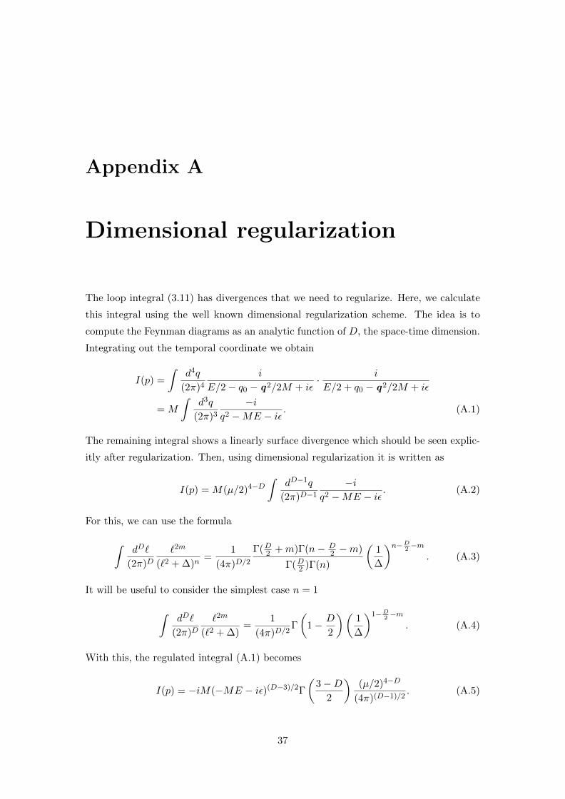
The loop integral (3.11) has divergences that we need to regularize. Here, we calculate
this integral using the well known dimensional regularization scheme. The idea is to
compute the Feynman diagrams as an analytic function of D, the space-time dimension.
Integrating out the temporal coordinate we obtain
I(p) =
∫d4q
(2π)4i
E/2− q0 − q2/2M + iε· i
E/2 + q0 − q2/2M + iε
= M
∫d3q
(2π)3−i
q2 −ME − iε. (A.1)
The remaining integral shows a linearly surface divergence which should be seen explic-
itly after regularization. Then, using dimensional regularization it is written as
I(p) = M(µ/2)4−D∫
dD−1q
(2π)D−1−i
q2 −ME − iε. (A.2)
For this, we can use the formula
∫dD`
(2π)D`2m
(`2 + ∆)n=
1
(4π)D/2Γ(D2 +m)Γ(n− D
2 −m)
Γ(D2 )Γ(n)
(1
∆
)n−D2−m
. (A.3)
It will be useful to consider the simplest case n = 1
∫dD`
(2π)D`2m
(`2 + ∆)=
1
(4π)D/2Γ
(1− D
2
)(1
∆
)1−D2−m
. (A.4)
With this, the regulated integral (A.1) becomes
I(p) = −iM(−ME − iε)(D−3)/2Γ(
3−D2
)(µ/2)4−D
(4π)(D−1)/2. (A.5)
37

Appendix A. Dimensional regularization 38
At D = 4 we do not find any pole. This drawback arises from the use of dimensional
regularization in this type of integrals. To see that, let us analyze the formula (A.3).
To resolve the more general integral on the left side of the Eq. (A.3) we use the integral
formulation of the Beta function
B(x, y) =
∫ ∞0
tx−1
(1 + t)x+ydt =
Γ(x)Γ(y)
Γ(x+ y)(A.6)
with x = d/2 + m and y = n − d/2 − m. However, this integral formulation can be
used consistently only when <[x] > 0 and <[y] > 0. In a four-dimensional space with
m = 0 and n = 2, x > 0 and in the y → 0 limit the integral formulation of the beta
function is still valid. So that, when d → 4− we see quickly that the integral on the
left side of (A.3) has a logarithmic surface divergence, and that the gamma function on
the right side goes to Γ(0+). This pole corresponds to the logarithmic divergence in the
momentum integral.
Now let us consider m = 2 and like before n = 2. The momentum integral on the left
side of (A.3) has a quadratic divergence while on the right side, the gamma function goes
to Γ(−1). As before, we could say that this pole corresponds to the quadratic divergence
in the momentum integral. Or more generally, we could say that the isolated poles of the
gamma function at z = 0,−1,−2..., correspond to the logarithmic, quadratic, quartic,
and so on, divergences in the momentum integral respectively.
However, dimensional regularization are designed to retain only the logarithmic diver-
gences. For example, the previous quadratic divergence was related to the gamma func-
tion evaluated at z = −1. Moreover, the formula zΓ(z) = Γ(z + 1) relates both poles,
Γ(0) and Γ(−1) by a simple constant. With this, we can always express any pole of the
gamma function as a constant times Γ(0), the pole corresponding to a logarithmic diver-
gence. Consequently, for quadratic, quartic and in general for even surface divergences,
the resulting regulated integral retain only the logarithmic divergence.
Looking carefully, for divergences greater than the logarithmic one, dimensional regu-
larization simply change the extra internal momenta by the external momenta. This is
clear if we regularize the more divergent loop integral (3.28),
I2m(p) =
∫d4q
(2π)4q2m
i
E/2− q0 − q2/2M + iε· i
E/2 + q0 − q2/2M + iε
= M
∫d3q
(2π)3q2m
−iq2 −ME − iε
. (A.7)
Using the formula (A.4) we obtain
I2m(p) = −iM(ME)m(−ME − iε)(D−3)/2Γ(
3−D2
)(µ/2)4−D
(4π)(D−1)/2. (A.8)
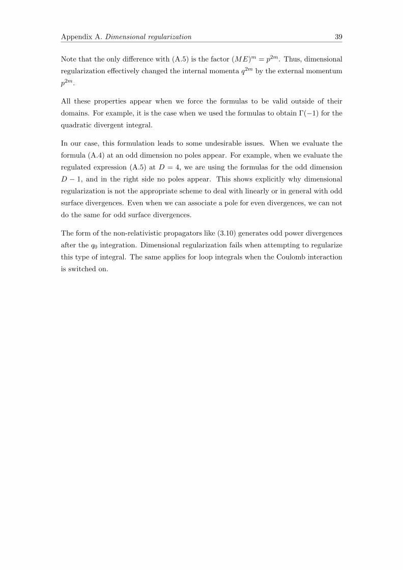
Appendix A. Dimensional regularization 39
Note that the only difference with (A.5) is the factor (ME)m = p2m. Thus, dimensional
regularization effectively changed the internal momenta q2m by the external momentum
p2m.
All these properties appear when we force the formulas to be valid outside of their
domains. For example, it is the case when we used the formulas to obtain Γ(−1) for the
quadratic divergent integral.
In our case, this formulation leads to some undesirable issues. When we evaluate the
formula (A.4) at an odd dimension no poles appear. For example, when we evaluate the
regulated expression (A.5) at D = 4, we are using the formulas for the odd dimension
D − 1, and in the right side no poles appear. This shows explicitly why dimensional
regularization is not the appropriate scheme to deal with linearly or in general with odd
surface divergences. Even when we can associate a pole for even divergences, we can not
do the same for odd surface divergences.
The form of the non-relativistic propagators like (3.10) generates odd power divergences
after the q0 integration. Dimensional regularization fails when attempting to regularize
this type of integral. The same applies for loop integrals when the Coulomb interaction
is switched on.

Appendix B
The Coulomb modified scattering
amplitude
Here, we calculate the Coulomb modified part of the scattering amplitude Eq. (4.2),
using the expression given by the Eq. (2.41),
TSC(p,p ′) =
∞∑n=0
〈χ(−)p |VS(G
(+)C VS)n|χ(+)
p′ 〉. (B.1)
The states |χ(+/−)p 〉 are the (outgoing/incoming) Coulomb state of momentum p defined
in the Eqs. (2.18) and (2.19),
χ(+)p (r) = e−
12πηΓ (1 + iη)M (−iη, 1, ipr − ip · r) eip·r , (B.2)
χ(−)p (r) = e−
12πηΓ (1− iη)M (iη, 1,−ipr − ip · r) eip·r . (B.3)
The operator G(+)C = 1/(Ep − H0 − VC + iε) is the Coulomb propagator, whose spectral
representation in terms of the Coulomb wave functions is
G(+)C (E) = 2µ
∫d3q
(2π)3|χ(+)
q 〉〈χ(+)q |
2µE − q2 + iε. (B.4)
The other ingredient in the calculation of the amplitude is the short-range local operator
VS derived from the effective Lagrangian Eq. (4.1), with C0 and C2 at the same leading
order. In momentum space it is given by
〈q |VS |p〉 = C0 +C2
2(q2 + p2). (B.5)
40

Appendix B. The Coulomb modified scattering amplitude 41
In order to calculate the expression for the modified scattering amplitude, we need to
insert the Eq. (B.5) into Eq. (B.1) in a separable way, i.e.;
〈q |VS |p〉 =3∑i=1
fi(q)gi(p) (B.6)
where fi(q) and gi(p) are the components of the following F and G vectors respectively,
F =
√C0√
C2/2 q2√C2/2
, G =
√C0√C2/2√
C2/2 p2
. (B.7)
With this, it is possible to rewrite the Eq. (B.1) in a matricial way
TSC(p,p ′) = AT · [1 +M +M2 + ...] ·B. (B.8)
The A and B factors are the three-component vectors
A =
√C0ψ
(−)∗0 (p)√
C2/2ψ(−)∗2 (p)√
C2/2ψ(−)∗0 (p)
, B =
√C0ψ
(+)0 (p′)√
C2/2ψ(+)0 (p′)√
C2/2ψ(+)2 (p′)
, (B.9)
whose components are in terms of the functions
ψ(−)∗2n (p) =
∫d3q
(2π)3χ(−)∗p (q)q2n, (B.10)
and
ψ(+)2n (p) =
∫d3q
(2π)3χ(+)p′ (q) q2n. (B.11)
The sequence in the brackets of Eq. (B.8) is a geometric series generated by M , where
M is the square matrix whose components are
Mij = 2µ
∫d3q
(2π)3
∫d3k
(2π)3
∫d3k′
(2π)3gi(k)
χ(+)q (k)χ
(+)∗q
(k ′)
2µE − q2 + iεfj(k
′). (B.12)
Assuming convergence, the next step is to resolve the geometric series generated by M
∞∑k=0
Mk =1
1−M. (B.13)
This means that the series equates the inverse matrix of D = 1−M .
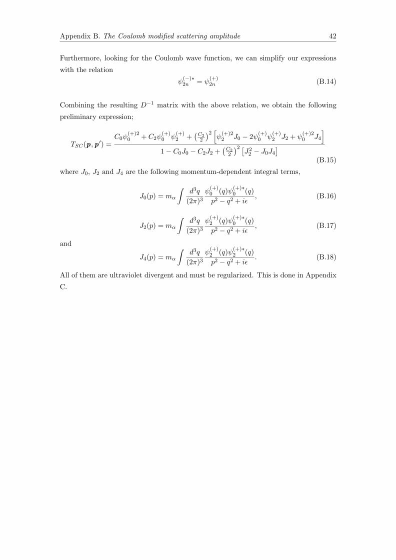
Appendix B. The Coulomb modified scattering amplitude 42
Furthermore, looking for the Coulomb wave function, we can simplify our expressions
with the relation
ψ(−)∗2n = ψ
(+)2n (B.14)
Combining the resulting D−1 matrix with the above relation, we obtain the following
preliminary expression;
TSC(p,p ′) =C0ψ
(+)20 + C2ψ
(+)0 ψ
(+)2 +
(C22
)2 [ψ(+)22 J0 − 2ψ
(+)0 ψ
(+)2 J2 + ψ
(+)20 J4
]1− C0J0 − C2J2 +
(C22
)2 [J22 − J0J4
](B.15)
where J0, J2 and J4 are the following momentum-dependent integral terms,
J0(p) = mα
∫d3q
(2π)3ψ(+)0 (q)ψ
(+)∗0 (q)
p2 − q2 + iε, (B.16)
J2(p) = mα
∫d3q
(2π)3ψ(+)2 (q)ψ
(+)∗0 (q)
p2 − q2 + iε, (B.17)
and
J4(p) = mα
∫d3q
(2π)3ψ(+)2 (q)ψ
(+)∗2 (q)
p2 − q2 + iε. (B.18)
All of them are ultraviolet divergent and must be regularized. This is done in Appendix
C.

Appendix C
Divergent integrals and
dimensional regularization
In this Appendix we regulate the integrals (B.16) to (B.18). Since these calculations
are very extensive, here we present the main steps of this calculation. Explanations are
given in order to alleviate the work for the reader.
Let us start by J0,
J0(p) = mα
∫d3q
(2π)3ψ(+)0 (q)ψ
(+)∗0 (q)
p2 − q2 + iε. (C.1)
To solve this, first we need to solve ψ(+)0 (q) defined in (B.11). Using dimensional regu-
larization we write
ψ(+)0 (q) =
(µ2
)ε ∫ dDk
(2π)Dχ(+)q (k) , (C.2)
where µ is the renormalization scale and ε = 3 −D. The integrand corresponds to the
Fourier-transformed Coulomb wave function
χ(+)q (k) =
∫d3rχ
(+)q (r) e−ik ·r . (C.3)
To carry out the integration we use the partial-wave expansion of the Coulomb wave
function Eq (2.25),
χ(+)q (r) =
∞∑l=0
il(2l + 1)eiσl(q)R+l (qr)Pl(cos θ). (C.4)
43

Appendix C. Divergent integrals and dimensional regularization 44
Using spherical coordinates k · r = kr[cos θ cos θ′ + sin θ sin θ′ cos(φ− φ′)] and thus
χ(+)q (k) =
∞∑l=0
il(2l + 1)eiσl(q)∫d3rR+
l (qr)Pl(cos θ)e−ikr[cos θ cos θ′+sin θ sin θ′ cos(φ−φ′)],
(C.5)
where the prime indicates the set for the momentum coordinate k . Without losing
generality we choose φ′ = 0. Thus, the integral over φ gives∫ 2π
0dφe−ikr sin θ sin θ
′ cosφ = J0(−kr sin θ sin θ′), (C.6)
where J0(−kr sin θ sin θ′) is the Bessel function of the first kind. For the integral over θ
we have∫ π
0dθ sin θPl(cos θ)J0(−kr sin θ sin θ′)e−ikr cos θ cos θ
′= il
√2π
−krPl(cos θ′)Jl+ 1
2(−kr).
(C.7)
Then, a partial result for the Fourier transformed Coulomb wave function is
χ(+)q (k) = 2π
∞∑l=0
il(2l + 1)eiσl(q)∫ ∞0
drr2R+l (qr)il
√2π
−krPl(cos θ′)Jl+ 1
2(−kr). (C.8)
Putting this into Eq (C.2) and commuting the integrations
ψ(+)0 (q) = 2π
∞∑l=0
il(2l + 1)(µ
2
)εeiσl(q)
∫ddk
(2π)d
∫ ∞0
drr2R+l (qr)il
√2π
−krPl(cos θ′)Jl+ 1
2(−kr)
=2π
(2π)d
∞∑l=0
il(2l + 1)(µ
2
)εeiσl(q)
∫drr2R+
l (qr)il∫ ∞0
dkk2−ε√
2π
−krJl+ 1
2(−kr)
×∫ 2π
0dφ′∫ π
0dθ′ sin θ′Pl(cos θ′). (C.9)
The integration over θ′ vanishes for l 6= 0 and for l = 0 it gives a factor 2. The integration
over φ′ gives a factor 2π. After that, for the integration in k we use the definition of the
spherical Bessel functions jl(z) for l = 0
j0(z) =
√π
2zJ 1
2(z), (C.10)
which is an even function allowing us to change the sign of the factor −kr and thus use
the result ∫ ∞0
dkk32−εJ 1
2(kr) = 2
32−εr−
52+εΓ
(32 −
ε2
)Γ(ε2
) . (C.11)

Appendix C. Divergent integrals and dimensional regularization 45
Then, for the integration over the radial coordinate we recall the expression for the radial
wave function R+0 (qr), which is given by the Eq. (2.27)
R+0 (qr) = Cηe
iqr1 F1(1 + iη, 2,−2iqr), (C.12)
and the following formula involving hypergeometric functions,∫ ∞0
rνe−µr 1 F1(a, b, qr) = Γ(ν + 1)µ−ν−1 2 F1(a, ν + 1, b; p/µ). (C.13)
When all the integrations are performed we obtain
ψ(+)0 (q) = 23−ε(2π)2−d
√π(µ
2
)εeiσ0
Γ(32 −
ε2
)Γ(ε2
) CηΓ(ε)(−iq)−ε 2 F1(1+iη, ε, 2; 2). (C.14)
Using the facts 2F1(1 + iη, 0, 2; 2) = 1 and Γ(ε)/Γ(ε/2) = 1/2 we finally have, in the
limit ε→ 0,
ψ(+)0 (q) = Cηe
iσ0 (C.15)
We now proceed to calculate J0(p). According to Eqs. (C.1) and (C.15)
J0(p) = mα
∫d3q
(2π)32πηq
e2πηq − 1
1
p2 − q2 + iε. (C.16)
This integral can be solved writing it in two parts, a finite and a divergent part,
J0(p) = mα
∫d3q
(2π)32πηq
e2πηq − 1
1
p2 − q2 + iε
[p2
q2− p2 − q2
q2
]= Jfin0 + Jdiv0 . (C.17)
For the finite part
Jfin0 = mα
∫d3q
(2π)32πηq
e2πηq − 1
1
p2 − q2 + iε
p2
q2, (C.18)
we perform the substitution x = A/q, where A = 2πkC , and we use the fact
limε→0+
[− p
2
A2− iε
]= lim
ξ→0+
p2
A2e−i(π−ξ) = lim
ξ→0+
[A
pei(π−ξ)/2
]−2= (2πiηq) = b−2, (C.19)
to rewrite it in the form
Jfin0 = −mαA
2π2
∫ ∞0
xdx
(ex − 1)(x2 + b2). (C.20)
The integral over x gives∫ ∞0
xdx
(ex − 1)(x2 + b2)=
1
2
[ln
(b
2π
)− π
b− ψ
(b
2π
)], (C.21)
Appendix C. Divergent integrals and dimensional regularization 46
where the ψ-function is the logarithmic derivative of the Γ-function. Thus, the finite
part becomes
Jfin0 = −mαA
4π2
[χ(iηp) +
1
2iηp− ln(iηp)
]= −mαkC
2πH(ηp). (C.22)
For the divergent part we perform dimensional regularization and PDS subtraction in
order to take into account extra divergences besides the logarithmic one. Using the same
substitution x = A/q and integrating over the angles we obtain
Jdiv0 = −mα
(µ2
)3−D ∫ dDq
(2π)D2πηq
e2πηq − 1
1
q2
= −mαµ3
4A2
(A2
πµ2
)D/21
Γ(n/2)
∫ ∞0
x2−D
ex − 1dx. (C.23)
For the integral over x we use the formula
ζ(s) =1
Γ(s)
∫ ∞0
xs−1
ex − 1dx, (C.24)
involving the gamma function Γ(s) and the Riemann zeta function ζ(s), giving for the
divergent part of J0 the following expression
Jdiv0 = −mαµ3
4A2
(A2
πµ2
)D/21
Γ(D/2)Γ(3−D)ζ(3−D). (C.25)
If we evaluate the above expression at D = 3 the zeta function becomes finite ζ(0) =
−1/2, but we gain a pole from the gamma function Γ(0) = ∞. This pole corresponds
to the logarithmic divergence present in the integral J0. However, this is not the only
pole that we find. For D = 2 the gamma function is finite but the zeta function diverges
ζ(1) = ∞. This pole corresponds to the linear divergence also present in J0. The
logarithmic divergence is obtained by expanding around ε = 3−D, when ε goes to zero.
Jdiv0 =mαkC
2π
[1
ε+ ln
(µ√π
2kC
)+ 1− 3
2γE
]. (C.26)
where γE = 0.5772... is the Euler’s constant.
Expanding around ε = 2−D we recover the linear divergence part from (C.18). For this
we obtain
δJdiv0 =mαµ
4π
1
D − 2. (C.27)
Appendix C. Divergent integrals and dimensional regularization 47
PDS regularization scheme tells us that this contribution should be subtracted from the
result (C.19) for the D → 3 limit. In this limit J0 takes the form
Jdiv0 =mαkC
2π
[1
ε+ ln
(µ√π
2kC
)+ 1− 3
2γE
]− mαµ
4π. (C.28)
Finally, from (C.22) and (C.28) we obtain
J0(p) =mα
4π
2kC
[1
ε+ ln
(µ√π
2kC
)+ 1− 3
2γE
]− µ− 2kCH(ηp)
. (C.29)
The next integral to solve is (B.17),
J2(p) = mα
∫d3q
(2π)3ψ(+)2 (q)ψ
(+)∗0 (q)
p2 − q2 + iε, (C.30)
which it is required to know ψ(+)2 (q) defined in (B.11) for n = 1. For this, we write
ψ(+)2 (q) =
(µ2
)ε ∫ dDk
(2π)Dχ(+)q (k) k2
=2π
(2π)D
∞∑l=0
il(2l + 1)(µ
2
)εeiσl(q)
∫ ∞0
drr2R+l (qr)il
∫ ∞0
dkk4−ε√
2π
−krJl+ 1
2(−kr)
×∫ 2π
0dφ′∫ π
0dθ′ sin θ′Pl(cos θ′). (C.31)
This expression is similar to the Eq. (C.9) for ψ(+)0 (q), except for the exponent 4 in k4−ε
just after the k-integral. As before, the integral over the angles will give us a factor of
4π while cancels all terms different from l = 0. After that, in order to use the formula
(C.11) to perform the integral over k, we must use the definition of the spherical Bessel
function Eq. (C.10) to change the sign of the factor −kr and use the properties of the
sine function to replace two k-powers in the integrand for two derivatives on r,
k2j0(kr) = −1
r
(d2
dr2
)rj0(kr). (C.32)
Then, we leave the derivatives on r out of the k-integral. After carrying out the integra-
tion over k using (C.11), we apply the r derivatives to the resulting expression. Finally,
the integration over r is performed using the formula (C.13). Thus we obtain
ψ(+)2 (q) = 24−ε(2π)2−D
√π(µ
2
)εeiσ0
Γ(52 −
ε2
)Γ(ε2
) CηΓ(−1+ε)(−iq)2−ε 2 F1(1+iη,−2+ε, 2; 2).
(C.33)

Appendix C. Divergent integrals and dimensional regularization 48
In the ε→ 0 limit the divergent terms cancel each other. So, using 2F1(1+iη,−2, 2; 2) =
1/3− 2η2/3 we have
ψ(+)2 (q) = Cηe
iσ0(q2 − 2k2C). (C.34)
However, there is a pole for smaller dimensions. Rewriting (C.33) for ε = 2−D
ψ(+)2 (q) = 23−ε(2π)2−D
√π(µ
2
)1+εeiσ0
Γ(2− ε
2
)Γ(12 + ε
2
)CηΓ(ε)(−iq)1−ε 2 F1(1+iη,−1+ε, 2; 2).
(C.35)
Now, in the ε→ 0 limit we use Γ(ε) = 1/ε and 2F1(1 + iη,−1, 2; 2) = −iη and then this
pole becomes
δψ(+)2 (q) = Cηe
iσ0 2kCµ
D − 2. (C.36)
Returning to the dimension D = 3, and subtracting (C.36) from (C.34) one has
ψ(+)2 (q) = Cηe
iσ0(q2 − 2k2C − 2kCµ). (C.37)
Note that, an useful relation is given by the Eqs. (C.15) and (C.37)
ψ(+)2 (q) = ψ
(+)0 (q)(q2 − 2k2C − 2kCµ). (C.38)
Now we proceed to calculate J2(p). According to the Eq. (B.16) and the relation (C.36),
J2(p) may be written as
J2(p) = (p2 − 2k2C − 2kCµ)J0(p)− I3, (C.39)
where I3 is a number given by the following integral
I3 = mα
∫d3q
(2π)32πηq
e2πηq − 1. (C.40)
This is similar to the integral (C.23). Dimensional regularization gives for this integral,
as well as (C.23), a result in terms of the gamma and zeta functions,
I3 =mαµ
3
4
(A2
πµ2
)D/21
Γ(D/2)
∫ ∞0
x−D
ex − 1dx
=mαµ
3
4
(A2
πµ2
)D/21
Γ(D/2)Γ(1−D)ζ(1−D). (C.41)
As we see, if we evaluate the expression for I3 at D = 3 we gain a pole from the
gamma function. However, the zeta function becomes zero. Therefore, expanding around
Appendix C. Divergent integrals and dimensional regularization 49
ε = 3−D, when ε goes to zero, we obtain
I3 = 2πmαk3Cζ′(−2). (C.42)
Now, looking again for (C.41) we see that it has a PDS pole at D = 2 from the gamma
function. This pole gives
I3,1 = −πmαk2C
µ
12. (C.43)
For D = 1, the gamma function in (C.41) diverges, so that the pole in this case is
I3,2 = mαkCµ2
8. (C.44)
For n = 0, the remaining pole is
I3,3 = −mαµ3
8. (C.45)
Subtracting these poles from (C.42), PDS gives for I3 the following expression
I3 = mα
(2πζ ′(−2)k3C +
π
12k2Cµ−
1
8kCµ
2 +µ3
8
). (C.46)
With this we have completed the calculation of J2(p).
To compute the final integral Eq. (B.18), we apply for this the same steps used to
calculate the above integrals. Firs, we rewrite it in terms of the less-divergent integrals
J0, J2 and I3, and in terms of the more divergent integral,
I5 = mα
∫d3q
(2π)32πηq
e2πηq − 1q2. (C.47)
With this, the integral J4 can be expressed as
J4(p) = (p2 − 2k2C − 2kCµ)J2(p) + (2k2C + 2kCµ)I3 − I5, (C.48)
Applying dimensional regularization as before, the new integral term I5 becomes
I5 =mαµ
3A2
4
(A2
πµ2
)D/21
Γ(D/2)
∫ ∞0
x−2−D
ex − 1dx
=mαµ
3
4
(A2
πµ2
)D/21
Γ(D/2)Γ(−1−D)ζ(−1−D). (C.49)

Appendix C. Divergent integrals and dimensional regularization 50
Expanding around ε = 3−D no pole is observed, so that
I5 =2
3π3mαζ
′(−4)k5C . (C.50)
Including the PDS D = 2, 1, 0,−1,−2 poles I5 becomes
I5 = mα
(2
3π3ζ ′(−4)k5C −
4π3k4Cµ
3−π2ζ ′(−2)k3Cµ
2
4+π2k2Cµ
3
24+π2kCµ
4
32− πµ5
16
)(C.51)
Thus, we have completed the calculations for the final divergent integral defined in
(B.18). To do that, we have used the PDS regularization scheme, in order to recover
divergences beyond the logarithmic one.
Bibliography
[1] F. Hoyle, Astrophys. J. Suppl. 1, (1954) 121.
[2] C. Cook, W.A. Fowler, C.C. Lauritsen, and T. Lauritsen, Phys. Rev. 107 (1957) 508.
[3] C.J. Hogan, Rev. Mod. Phys. 72 (2000) 1149; A.N Schellekens, Rev. Mod. Phys. 85
(2013) 1491.
[4] M. Chernykh et al., Phys. Rev. Lett. 98 (2007) 032501.
[5] Y. Suzuki et al., Phys. Lett. B659 (2008) 160.
[6] R. de Diego, E. Garrido, D.V. Fedorov, and A.S. Jensen, Phys. Lett. B695 (2011)
324.
[7] Eric Braaten and H.-W. Hammer, Phys. Rep. 428 (2006) 259; R. Higa, Mod. Phys.
Lett. A 24 (2009) 915.
[8] S. Weinberg, Physica 96 A (1979) 327.
[9] S. Weinberg, Phys. Lett. B 251 (1990) 288; Nucl. Phys. B 363 (1991) 3.
[10] P.F. Bedaque and U. van Kolck, Ann. Rev. Nucl. Part. Sci. 52 (2002) 339; E.
Epelbaum, H.-W. Hammer and U.-G. Meissner, Rev. Mod. Phys. 81 (2009) 1773.
[11] D.B. Kaplan, J.-W. Lee, D.T. Son, and M.A. Stephanon, Phys. Rev. D 80 (2009)
125005; H.-W. Hammer and B.G. Swingle, Ann. Phys. 321 (2006) 306; H.-W. Ham-
mer and R. Higa, Eur. Phys. J. A 37 (2008) 193.
[12] R. Higa, H.-W. Hammer, and U. van Kolck, Nucl. Phys. A 809 (2008) 171.
[13] E.P. Wigner, Phys. Rev. 98 (1955) 145; H.-W. Hammer and D. Lee, Phys.Lett.
B681 (2009) 500; Annals Phys. 325 (2010) 2212.
[14] D.B. Kaplan, M.J. Savage, and M.B. Wise, Nucl. Phys. B 534 (1998) 329.
[15] X. Kong and F. Ravndal, Nucl. Phys. A 665 (2000) 137.
51

Bibliography 52
[16] L. D. Landau and E. M. Lifschitz, Quantum Mechanics (Non-relativistic theory),
Pergamon Press, London, 1958.
[17] John M. Blatt and Victor F. Weisskopf, Theoretical Nuclear Physics, John Wiley
and Sons, Inc., New York, 1952.
[18] S. Weinberg, Lectures on Quantum Mechanics, Cambridge University Press, New
York, 2013.
[19] G. Arfken, Mathematical methods for physicists, Academic Press, Inc., San Diego,
California 1985.
[20] H.A. Bethe, Phys. Rev. 76 (1949) 38.
[21] L.P Kok, J.W. de Maag, H.H. Brouwer, and H. van Haeringen, Phys. Rev. C 26
(1982) 2381.
[22] F.L. Yost, J.A. Wheeler, and G. Breit, Phys. Rev. 49 (1936) 174.
[23] A. Sommerfeld, Atombau and Spektrallinien, volume II, Vieweg, Braunschweig,
1939.
[24] M.L. Goldberger and K.M. Watson, Collision Theory, John Wiley and Sons, New
York, 1967.
[25] A. Deltuva, A.C. Fonseca, and P.U. Saver, Phys. Rev. C 71 (2005) 054005; 72 (2005)
054004.
[26] W. Glockle, The Quantum Mechanical Few-Body Problem, Springer-Verlag Berlin
Heidelberg, Berlin, 1983.
[27] L. Landau, Ya. Smorodinsky, J. Phys. Acad. Sci. USSR 8 (1944) 154.
[28] J. Hamilton, I. Overbo, and Tromborg, Nucl. Phys. B 60 (1973) 443.
[29] G.A. Miller, B.M.K. Nefkens, and I. Slaus, Phys. Rep. 194 (1990) 1.
[30] P.F. Bedaque, H.-W. Hammer, U. van Kolck, Phys. Lett. B 569 (2003) 159.
[31] D.B. Kaplan, arXiv:nucl-th/9506035; arXiv:nucl-th/9901003; A. Pich, arXiv:hep-
ph/9806303; J. Bain, http://ls.poly.edu/ jbain/papers/EFTs.
[32] K.G. Wilson, Phys. Rev. D (1971) 3.
[33] S. Weinberg, The Quantum Theory of Fields, volume II, Cambridge University
Press, New York, 1996.
[34] J. Gasser and H. Leutwyler, Annals Phys. 158 (1984) 142.

Bibliography 53
[35] S. Scherer, Adv. Nucl. Phys. 27, 277 (2003).
[36] C. Ordonez, L. Ray, and U van Kolck, Phys. Rev. Lett. 72 (1994) 1982; Phys.
Rev. C. 53 (1996) 2086; E. Epelbaum, Prog. Part. Nucl. Phys. 57 (2006) 654; E.
Epelbaum, H.-W. Hammer, and U.-G. Meissner, Rev. Mod. Phys. 81 (2009) 1773.
[37] D.B. Kaplan, M.J. Savage, and M.B. Wise, Nucl. Phys. B 478 (1996) 629; D.B.
Kaplan, M.J. Savage, and M.B. Wise, Phys. Lett. B 424 (1998) 390; D.B. Kaplan,
Nucl. Phys. B 494 (1997) 471.
[38] G. ’t Hooft, Nucl. Phys. B 61 (1973) 445.
[39] S. Weinberg, Phys. Rev. D 8 (1973) 3497.
[40] D.R. Phillips, S.R. Beane and T.D. Cohen, Ann. of Phys. 263 (1998) 255.
[41] C. Itzykson and J. Zuber, Quantum Field Theory, McGraw-Hill Inc., New York,
1980.
[42] J.E. Beam, Phys. Rev. 158 (1967) 907.
[43] Chart of nuclides, http://www.nndc.bnl.gov/chart/reCenter.jsp?z=1n=1.
[44] Nuclear Data Evaluation Project Triangular Universities Nuclear Laboratory,
http://www.tunl.duke.edu/nucldata/index.shtml.
[45] J.A. Wheleer, Phys. Rev. 62 (1937) 1083.
[46] M.V. Zhukov, B.V. Danilin, D.V. Fedorov, J.M. Bang, I.J. Thompson, and J.S.
Vaagen, Phys. Rep. 231 (1993) 151; K. Riisager, Rev. Mod. Phys. 66 (1994) 1105.
[47] T. Federico, A. Delfino, L. Tomio, and M. Yamashita, Prog. Part. Nucl. Phys. 67
(2012) 939.
[48] B.A. Brown, A. Csoto, and R. Sherr, Nucl. Phys. A 597 (1996) 66; H. Esbensen
and G.F. Bertsch, Nucl. Phys. A 600 (1996) 37.
[49] C.A. Bertulani, H.-W. Hammer, U. van Kolck, Nucl. Phys. A 712 (2002) 37.
[50] C.A. Bertulani, R. Higa, U. van Kolck, in preparation.
[51] S.A. Afzal, A.A.Z. Ahmad, S. Ali, Rev. Mod. Phys. 41 (1969) 247.
[52] S. Konig, D.Lee, and H.-W. Hammer, J. Phys. G 40 (2013) 045106.