1

The mystery of alpha spectroscopyIt has been said that alpha spectroscopy is more of an art than a science. Alpha spectroscopy, an art, not a science? The American Heritage® Dictionary of the English Language defines art as “skill that is attained by study, practice, or observation: the art of the baker; the blacksmith’s art”. Radiochemists can relate to that definition and would agree that “the art of the radiochemist” could be easily inserted into the definition when speaking of alpha spec sample preparation. So what is all the mystery about? This application note will take you on a journey to simplify and explain the complexities, i.e., mystery, of alpha spectroscopy that cause practitioners to call it an art form, rather than a science. The intent of this note is not to provide full technical explanations, but rather simple and concise explanations to complex and often-misunderstood theories related to alpha spectroscopy.

Sample preparation – it’s more than just weighing samples? Let’s begin by comparing alpha spectroscopy to gamma spectroscopy, a field that is fairly straightforward and more easily understood. Let’s say I have a soil sample that requires gamma analysis. Prior to counting, I need to weigh an appropriate amount of sample, place it in a container shape that matches a calibration file stored in my counting software and count it – straightforward and simple, right? Okay, even though this explanation is somewhat of an over-simplification, it accurately describes the gamma sample preparation process – basically weigh it (or measure the volume) and count it. Now, what if that same soil sample requires alpha analysis too? The process of preparing the sample for alpha spectroscopy analysis becomes increasingly more difficult.

Why?

When Ernest Rutherford first identified and named the alpha particle, his tests showed that it was merely the nucleus of a helium atom. The general equation for alpha decay is shown below, where P = parent nucleus and D = daughter nucleus. A = number of protons and neutrons in the nucleus while Z is the atomic number or number of protons.

Why is that important? Take note of the atomic number of 226Ra during decay. The atomic number decreases by two units due to the +2 alpha charge, hence giving us a reason to call an alpha particle a “charged particle”. This is a key phrase in helping us understand the alpha particle. Charged particles, like alpha particles, have definite and fixed ranges, as opposed to photons, i.e., gamma rays that do not have fixed ranges.

So what does range have to do with counting soil samples? In our example, range can best be described as the distance an alpha particle can travel in the soil sample and be ‘counted’ before it loses all of its energy and goes undetected by our counting instrument.

How far can an alpha particle travel? The answer is – not very far. Because of their limited range, alpha particles are completely stopped by the dead layer of skin on our bodies or a single sheet of paper; even air can stop them. Any alpha particles within the soil sample would be stopped by the soil itself and never detected by our counting instrument. Only the few alpha particles on the surface of the soil could be detected. For that reason, all types of samples, soils, filters, waters, oils, urine, etc., must undergo some type of treatment before they can be counted, i.e., detected by any alpha spectroscopy based instrument. The three basic chemical procedures or treatments that alpha samples must undergo before counting are:

• Sample Preparation

• Chemical Separation

• Sample Mounting

Alpha Spectroscopy – An Art or a Science?

Ernest Rutherford 1871–1937

Application Note

2

Chemical Procedures – the mystery lies within

We’ve already determined that direct counting of samples for alpha spectroscopic analysis is not possible due to an alpha particle’s limited range. This fact is based purely on physics principles and quite easily understood. However, our first topic, sample preparation, muddies the physics water with some chemistry. Now, mix in different types of sample matrices, such as soils, waters and filters, and even more confusion is added. This is where most physicists stop listening and where much of the mystery surrounding alpha spec lies. Let’s simplify.

Sample Preparation Sample preparation is usually different for each type of sample matrix. For example, water samples usually undergo a co-precipitation technique which preconcentrates all actinides (the alpha emitting elements, such as thorium, uranium, neptunium, plutonium and americium, to name a few of the well known) in the sample. Soil samples usually require a more rigorous technique called fusion, or sometimes only a leaching technique is necessary. However, all sample preparations are designed to do one thing – remove as many impurities from the sample as possible and convert it into a form, usually an acidified liquid, suitable for subsequent chemical procedures. These procedures include chemical separation and mounting of the sample which is frequently called an unknown.

Note: From this point forward, for clarity, we will refer to the “sample” as the “unknown”.

Chemical Separation There are numerous methods and products available to aid in chemical separations. But before we discuss those, you may be asking why we need to chemically separate? The best way to describe this is with an example.

Let’s say we have an unknown that requires analysis for 241Am and 238Pu. 241Am has an energy of 5486 keV (main peak) and 238Pu has an energy of 5499 keV (main peak) – a separation of 13 keV. Those of you familiar with gamma spec are probably saying, “What’s the problem? “ The problem with alpha spec is technology – namely a limitation in the detector technology. CANBERRA’s Alpha Series of Passivated Implanted Planar Silicon (PIPS®) Detectors are the most advanced products in semi-conductor technology for alpha spec counting. The super thin window allows for optimal resolution at the close distances needed for high efficiency alpha counting, but there is still a limit. The best alpha detectors available today can only resolve (distinguish between) peaks greater than 17 keV apart, under ideal counting conditions and with a commercially prepared source. In our example of 241Am and 238Pu, the difference is 13 keV, thus the need for chemical separation.

So how does chemical separation work? Technically speaking, it depends on the type of separation – co-precipitation, liquid-liquid extraction, ion exchange, or extraction chromatography, or some combination of these.

However, we said we would not be so technical, so here is a simplistic view. If we need to analyze an unknown for Plutonium isotopes – 238, 239/240, we should perform a method that is optimized to remove all interfering radioactive isotopes which could negatively impact our spectral analysis. One of these is 241Am. Our chemical separation also needs to remove any other inorganic or organic matter that could interfere with the chemistry of our method. Chemical separation concentrates and purifies our sample for the element or elements we need to measure.

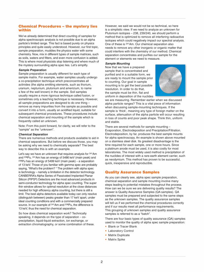
Sample Mounting Now that we have a prepared sample that is concentrated and purified and in a suitable form, we are ready to mount the sample prior to counting. Our goal in sample mounting is to get the best possible resolution. In order to do that, the sample must be thin, flat and uniform in deposition of the nuclides we are measuring. Remember earlier when we discussed alpha particle ranges? This is a vital piece of information when discussing sample-mounting techniques. If the sample is ‘thick’, meaning any type of foreign matter on the surface, attenuation of the alpha particle will occur resulting in loss of counts and poor peak shape. Think thin, uniform and stable.

There are several methods for sample mounting – Evaporation, Electrodeposition and Precipitation/Filtration. Electrodeposition, by far, produces the best sample mounts for alpha spectroscopy. An example is shown above mounted on a stainless steel disk. Its greatest disadvantage is the time required for each sample, one or more hours. Since a platinum anode must be used, it is also costly for most laboratories. The most widely used method is precipitation of the nuclides of interest with a rare-earth element carrier, such as neodymium. This method has proven to be successful, quick, inexpensive and reproducible.

Quality Assurance Samples

As you can clearly see, alpha spec sample preparation, chemical separation and sample mounting involve many steps leading to potential mistakes throughout the process. How can we be sure we are delivering quality results? The answer is Quality Assurance Samples (QA samples). QA samples must be prepared and subjected to the same steps as the unknown samples. The quality assurance samples will tell us if we performed the chemical procedures correctly and if our results meet all performance requirements. This grouping of unknown samples and quality assurance samples is referred to as a “batch”.

There are four basic types of quality assurance (QA) samples used to monitor the quality of alpha spec sample preparation: • Blank or Tracer Blank

• Laboratory Control

• Matrix Duplicate

• Matrix Spike

3

Since much of the work for alpha spectroscopy is client-driven, and each client will specify the level of quality control necessary for data validation purposes; the radiochemist needs flexibility when creating a batch. Usually a “batch” consists of no more than 20 unknown samples and one or more quality assurance samples. By definition, a “batch” of samples typically has the same sample matrix, such as soil; and is usually being prepared to analyze a single element of interest, such as Uranium. For example and as shown in Figure 1, CANBERRA’s Apex-Alpha™ Software, allows the radiochemist to select the number of unknowns, choose the sample matrix, and include one or more types of quality assurance samples when creating a batch.

Method Blanks and Tracer Blanks – to spike or not to spike? Method Blanks and Tracer Blanks are the easiest QA samples to understand. A Method Blank is just that, blank or empty. It is a sample known to be free from any radioactive element. De-ionized water is the typical choice. Why do you need it? Since we are dealing with radioactivity, we need to ensure that we are not spreading any radioactivity in the lab, otherwise known as contamination. So it’s that simple. The Method Blank will tell us if there is any contamination in our glassware, chemical reagents or any other lab supplies and equipment used during the preparation process. It can also tell us if we have Good Laboratory Practice (GLP). In other words, it can tell us if our glassware is washed properly, equipment is clean, reagents are uncontaminated, etc. If there is contamination in the Method Blank, we must assume that our unknown samples are possibly contaminated as well. A ‘contaminated’ blank usually dictates that the entire batch of samples be re-processed.

Figure 1: Apex-Alpha Batch Creation Screen.

Okay, that takes care of Method Blanks but what about Tracer Blanks? Tracer Blanks are also referred to as Reagent Blanks. Tracer Blank is similar to the Method Blank in that it is usually de-ionized water, but the radiochemist adds a radioactive tracer isotope to the sample. A little confusing since we just learned that a Method Blank was used to determine if any contamination was present. Now we’re adding radioactivity to a Blank? Confusing? Not really. Understanding a Tracer Isotope, usually called only Tracer, and why it’s used will help explain.

Tracers – Otherwise Known as Sanity Checks Our goal is to ultimately measure how much and what kind of alpha particles are in our unknown samples. Since we

are starting with an unknown, we need a marker or sanity check to help us determine if we are on the right track in identifying isotopes. The Tracer is a good tool for this. The radiochemist selects a Tracer for an element being analyzed, such as Plutonium, but not an isotope expected to be found in the unknown. For example, if our isotopes of interest (what we need to identify and measure) are 238Pu and 239Pu, we might choose 236Pu for the Tracer. A known amount of 236Pu would then be added to all unknowns and QA samples in the batch. 236Pu will behave chemically the same as our isotopes of interest, 238Pu and 239Pu. Therefore, a chemical yield or recovery can be calculated for each unknown and QA sample based on the ratio of known amount of Tracer we added versus the measured amount of Tracer we counted with our instrumentation. Determining chemical yield or recovery is the main purpose of a Tracer.

Now, back to the Tracer Blank. A Tracer Blank includes de-ionized water and a known amount of a radioactive isotope not expected to be in the unknown samples. So what will the analysis of the Tracer Blank tell us? If we added 100 dpm of 236Pu to our Tracer Blank, we should expect a 100% yield if we performed all the chemical steps perfectly. So, one piece of information we get from the Tracer Blank is how well our methods perform without any interference from the sample matrix. There is also a second and more important use for the Tracer Blank. Whenever a radioactive component is introduced into any sample, the risk for interference is possible. Some Tracer Isotopes may eventually cause interference in the isotopes of interest regions due to the natural decay process. The Tracer Blank spectrum, when analyzed, will show this interference.

Since we are adding Tracer to our unknown samples too, we can assume that the amount of interference detected in the Tracer Blank is equivalent to the amount of interference in the unknown samples. Based on this information, the Tracer Blank with its interference is subtracted from the unknown sample spectra. CANBERRA’s Apex-Alpha Software uses the following equation to subtract any possible interference.

4

Net Sample Counts = (S – SB) – (T – TB)

S = Sample Counts

SB = Sample Chamber Background Counts

T = Tracer Blank Counts

TB = Tracer Blank Chamber Background Counts

With this algorithm in place, the Tracer Blank can be counted in a different chamber than the sample, but the backgrounds for each of these spectra come from the same chambers each was counted in. The counts are normalized based on the tracer peak area in both the sample spectrum and the Tracer Blank spectrum in case there are not identical amounts of Tracer in each sample.

Generally, radiochemists will choose either the Blank or Tracer Blank, based on the type of Tracer solution used in the specific method, or at the request of their client. There are some elements, such as 237Np, that do not have an alpha-emitting tracer choice. In these cases, an external factor must be used to calculate a recovery. CANBERRA’s Apex-Alpha Software allows for an external recovery factor for each unknown sample as shown in Figure 2.

Laboratory Control Samples (LCS) – Accuracy Is What Matters Think of the Laboratory Control Sample as a test. A test is a critical examination, observation, or evaluation. Quite simply, a LCS will tell you if you passed or failed all the chemistry steps required for alpha spectroscopy. So what is a LCS? It is a sample that contains de-ionized water, a known quantity of Tracer, and a known quantity of the isotopes of interest. If our isotopes of interest are 238Pu and 239Pu, a known amount of one or both of these isotopes is added to the LCS, along with the same 236Pu tracer solution we discussed earlier. The LCS is considered the ‘perfect’ sample since it uses de-ionized water, and any possible matrix interference is eliminated. Ideally, if each sample

Figure 2: Batch Screen Showing External Recovery Entry.

preparation step is performed properly, the LCS should indicate a 100% recovery. If our LCS shows inaccurate results, we must assume that our chemistry methods have failed for some reason. This failure could be from analyst error, method failure or a combination of both. A poor LCS result should initiate an investigation to determine the cause of the failure. Since Laboratory Control Samples are the most comprehensive way to verify the accuracy of a method, tracking their performance over time is an invaluable tool for the radiochemist. CANBERRA’s Apex-Alpha Software can store and display Quality Control charts for all Procedures defined in the software. An example control chart for a 238Pu LCS series is shown in Figure 3. The example shows results one might expect from a properly run laboratory – recoveries close to, but not exceeding, 1 (or 100%).

Storing and tracking LCS data over time aids the radiochemist’s investigation in determining the root cause of an accuracy failure. As stated earlier, the failure could be based on something as simple as a new technician in the lab or a bad lot of reagents. However, when the chart shows a trend away from data that is expected, it is time to review lab

processes in more detail to get the analyses back on track.

Matrix Duplicate Samples – Precisely Important As if accuracy weren’t enough; we need to be precise too! The Matrix Duplicate Sample, usually called Duplicate or Dup, gives the radiochemist some important information about the batch. Basically, the duplicate is a ‘copy’ of one of the unknown samples. If the lab receives one bottle of an unknown water sample, the radiochemist will remove two sample aliquots from the bottle, label them accordingly and analyze them in an identical manner to perform the Matrix Duplicate analysis. The results for the two samples should be the same, or within reasonable uncertainty margins. If the results are not favorable, we can assume that our ability to reliably produce solid results is questionable.

Because precision is a statistically based calculation, and statisticians love math, there

are several ways to calculate and analyze the precision of the results from our duplicate samples. The radiochemist can face numerous precision calculation requests due to various clients’ specific requirements. The requirements are typically based on one or more of the following criteria: comparison to historical data from the same types of samples, client’s data reviewer preference or data set consistency for a particular project.

CANBERRA’s Apex-Alpha Software simplifies this “statistics” problem by offering the radiochemist the flexibility to select any of the three most popular types of Duplicate Equations (RPD, RER, or NAD) for each sample batch. The Batch Creation Screen in Figure 4 shows how an equation is selected for a particular batch if desired.

5

Of the three types of Duplicate Equations, the Relative Percent Difference (RPD) is the simplest and the one that is most often used. It calculates a percent difference between the two sample results. Typically, labs will set upper limits based on sample matrices. For example, for water samples, a 5% RPD might be acceptable for a batch. Whereas, for the more complicated soil samples, a 10% RPD, could be acceptable. The equation is as follows:

RPD = x 100%

S = Sample Result D = Duplicate Result

The Relative Error Ratio (RER), sometimes called Duplicate Error Ratio (DER), factors the uncertainties from both the unknown and duplicate sample into the equation. Remember what we said about statisticians – they love math. The desired result for the RER approaches 1. The equation is found below.

RER or DER = S = Sample Result D = Duplicate Result σs = sample uncertainty σs = duplicate uncertainty

Normalized Absolute Difference (NAD) is similar to the RER, and the equation is found below. As you can see, the uncertainties are handled somewhat differently in the two equations.

NAD =

S = Sample Result D = Duplicate Result σs = sample uncertainty σs = duplicate uncertainty

In summary, the Duplicate calculations are used to determine reproducibility of results. Each equation offers the data reviewer a unique way of comparing and contrasting data sets.

Figure 3: Quality Control Chart for 238Pu Laboratory Control Samples.

Figure 4: Batch Screen with Duplicate Equation options highlighted.

S – DS

S – D2σs + 2σd

S – D√σs

2 + σd2

6

Matrix spike – A Laboratory Control Sample look-alike The Matrix Spike, usually called a Spike, is the same as a LCS. However, instead of de-ionized water, an unknown sample aliquot is used. Simply put, the Spike result will show if there is a bias in the method for a particular element and matrix combination. For example, the same Uranium chemistry separation method may be used for both water samples and urine samples in the laboratory. This seems reasonable since they are both liquids. However, what if the Spike Sample yields from the water samples are always greater than the yields for urine samples? Is my method flawed? Did the analyst make a mistake? This is where a good Quality Control Program pays off. The Laboratory Control Sample yield from the batch should be compared to the Matrix Spike Sample yield. If the LCS is acceptable, but the Matrix Spike yield is not, we can assume that the urine matrix has introduced some type of interference. Further to our analysis, historical data can be used to demonstrate that a urine matrix routinely produces yields lower than water.

CANBERRA’s Apex-Alpha software equips the radiochemist with tools for easy retrieval of historical QA data for comparison. The QA data selection screen is shown in Figure 5. A pair of data charts of Matrix Spikes for an element (232U) in two matrices (water and urine, respectively) can be seen in Figure 6. The data does indeed show a recovery trend for water samples of about 98% versus a recovery in urine samples of about 91%.

The Matrix Spike result is just another piece of valuable information the radiochemist can use in determining the quality of the results. It can also be used to set expectations for the yields with various matrices based on historical data.

Figure 6: QA Data Charts showing Recovery for Water and Urine Matrices.

Last word on ChemistryIn the gamma spec world, our most fundamental concern in obtaining quality results is the proper calibration of the detector and electronics. Although that is equally important

in alpha spec, the most important factors in obtaining quality results are proper sample preparation, reproducible radiochemical separation, and mounting techniques that produce thin, uniform samples. More than any other factor, the chemistry dictates the quality of the result. Because these chemistry methods require hundreds of individual steps performed by numerous analysts in the lab, alpha spectroscopy data typically undergoes far more scrutiny by data reviewers than most other types of data generated by the lab. This scrutiny necessitates the use of the various types of Quality Assurance samples we have discussed. Even though they may be time consuming and costly to prepare, they are absolutely necessary to validate alpha spectroscopy results.

Figure 5: QA Data Selection Screen.

7

Figure 7: Data Review Set-up Screen.

Figure 8: Data Review Search Screen.

Beyond the Chemistry – Data ReviewGenerally speaking, most labs have a rigorous and strict peer review process for data prior to it being released to the client. Most often, this peer review process is enforced manually, using a cover sheet attached to the data set being reviewed. CANBERRA’s Apex-Alpha Software eliminates the manual paper trail and offers an electronic peer review process that can be enforced by the software. Sample results cannot be approved unless the user-specified level of peer review has been fulfilled, reducing the potential of releasing incorrect data. Figure 7 shows the Data Review Set-up Screen for Apex-Alpha.

Even though the peer review process uncovers most flagrant mistakes, clients subject the data to their own data verification and validation (V&V) process. When questions arise, the lab needs to respond quickly and efficiently to ensure lab accreditation is maintained. Often, this means

retrieving large amounts of historical data to investigate a possible problem. This task is usually very burdensome for most labs. Apex-Alpha Software relieves the burden by allowing the analyst to quickly and efficiently retrieve any result and spectrum counted in the system as can be seen from the Data Review Search Screen in Figure 8.

Whether an entire batch or a single sample result is needed, Apex-Alpha can locate the results in a matter of seconds, instead of hours or even days. After the sample result has been located, the investigation begins. There can be numerous reasons for a questionable result. However, incorrect placement of the Region of Interest (ROI) markers

is one of the most common mistakes in alpha spectroscopy analysis. The reason for this is based on a principle we learned earlier, the alpha particle is easily attenuated. This attenuation potential consequently causes a ‘low tail’ on the low energy side of the alpha peak. This tailing can be caused by many factors during the preparation phase. Only extreme attenuation cases merit a ‘re-analysis’ (a second preparation, separation and mounting) of the sample. In most cases, an adjustment of the ROI markers is all that is necessary.

CANBERRA’s Apex-Alpha software was designed specifically for this action. In Figure 9, notice the comprehensive “Shift All ROIs” and “Shift only Left Marker” slider controls and

other ROI control buttons available to the analyst. The ROI shift “short cuts” can be used to adjust all ROIs in a spectrum the same way, or each ROI can be adjusted separately at the discretion of the reviewer. In the example, the left ROI markers need to be shifted slightly to the left to include all the counts for the peaks.

8

Cradle to Grave – more science than artMost people have heard the phrase “cradle to grave” when referring to the data validation and verification process. The birth of a sample begins at sample collection, and death occurs when the client approves and accepts the sample result. The V&V process includes proving the results are accurate throughout the entire journey. As we have seen, the period between the cradle and the grave is a very long journey for the alpha spec sample (and for the alpha spectroscopist as well). Although the V&V process is not unique to alpha spec, the nature of the alpha particle and the complex chemistry associated with it dictate the need for a more rigorous V&V process. So, by now, we should be able to appreciate that there is a scientifically based reason for all the mystery and often misunderstood chemistry methods and QA requirements surrounding alpha spec. Alpha spectroscopy – it’s not so mysterious after all. More science than art? You might agree that it is a little of both.

Figure 9: Spectral Data Review Screen.

Bibliography1. Basic Radiation Protection Technology, 3rd Edition.

Daniel A. Gollnick, 1994 Pacific Radiation Corporation.

2. Radiation Detection and Measurement, 2nd Edition. Glenn F. Knoll, 1989 John Wiley and Sons, Inc.

3. Technical Brief – Sample Preparation for Alpha Spectroscopy, CANBERRA Industries.

4. Application Note – Data Validation Requirements for Low Level Alpha Spectroscopy, CANBERRA Industries.

5. Merriam-Webster – online dictionary.

6. The American Heritage® Dictionary of the English Language – online dictionary.

PIPS is a registered trademark of Mirion Technologies, Inc. and/or its affiliates in the United States and/or other countries.

C30202 - 11 /2006

Radiation Safety. Amplified. www.canberra.com Part of Mirion Technologies