alternating current studies and kinetic analysis of
TRANSCRIPT

Portland State University Portland State University
PDXScholar PDXScholar
Dissertations and Theses Dissertations and Theses
6-5-1984
Alternating current studies and kinetic analysis of Alternating current studies and kinetic analysis of
valinomycin mediated charge-transport through lipid valinomycin mediated charge-transport through lipid
bilayer membranes bilayer membranes
Kenneth Lee Cox Portland State University
Follow this and additional works at: https://pdxscholar.library.pdx.edu/open_access_etds
Part of the Biological and Chemical Physics Commons
Let us know how access to this document benefits you.
Recommended Citation Recommended Citation Cox, Kenneth Lee, "Alternating current studies and kinetic analysis of valinomycin mediated charge-transport through lipid bilayer membranes" (1984). Dissertations and Theses. Paper 3380. https://doi.org/10.15760/etd.5253
This Thesis is brought to you for free and open access. It has been accepted for inclusion in Dissertations and Theses by an authorized administrator of PDXScholar. Please contact us if we can make this document more accessible: [email protected].

AN ABSTRACT OF THE THESIS OF Kenneth Lee Cox for the Master
of Science in Physics presented June 5, 1984.
Title: Alternating.Current Studies and Kinetic Analysis of
Valinomycin Mediated Charge-Transport through Lipid
Bilayer Membranes.
APPROVED BY f·/IEMBE:lS OF THE THESIS COMMITTEE:
Arnold Pickar, Chairman
In this study we have investigated the frequency depen
dence of bilayer lipid membranes for a series of glyceryl
monoolein/n-decane bilayers in various aqueous ionic solu
tions containing the ionophore valinomycin. Reliable values
of membrane capacitance and conductance were obtained over
the frequency range 0.2 - 200 KHz using an automatic balancing
bridge under the control of a microprocessor unit. The ad
mittance data was then normalized and curve-fitted to pro-
duce relaxation times and amplitudes from which the kinetic

2
rate parameters, as deduced from a single slab dielectric
membrane model, were calc~~ted. These ac experimental rate
constants were then compared with those obtained from charge-
pulse relaxation methods.
It is shown that the values of the rate constants de-
rived from alternating current measurements differ signifi-
cantly (t>.05) with those obtained from the charge-pulse
exneriments. However, the rate constants do exhibit similar
trends with changes in the experimental conditions. The dis-
crepancies are most serious for the lowest metal ion concen-
tration (0.01 M RbCl) and particularly for the loaded carrier
translocation rate constant.
In view of these discrepancies and the prototypical na-
ture of this study various possible sources of experimental
error are discussed as well as the additional refinement of
the kinetic model to reflect a three slab dielectric membrane.
Such considerations still do not fully reconcile the ac results
with those from charge-pulse studies. Therefore, these dif-
ferences may imply that the membrane kinetic model requires v
farther modification. Several such model changes and experi-,,.,...
mental modifications are briefly discussed.

ALTERNATING CURRENT STUDIES AND KINETIC ANALYSIS
OF VALINCMYCIN MEDIATED CHARGE-TRANSPORT
THROUGH LIPID BILAYER MEMBRANES
by
KENNETH L. COX
A thesis submitted in partial fulfillment of the requirements for the degree of
MASTER OF SCIENCE in
PHYSICS
Portland State University
l 98 4-

TO THE OFFICE OF GRADUATE STUDIES AND RESEARCH:
The members of the Committee approve the thesis of
Kenneth Lee Cox presented June 5, 1984.
Arnold Pickar, Chairman
Pavel Smejtek t
APPROVED:
Raymond Sommerfeldt, Di~ector, Physics
Studies and Research

ACKNONLEDGEMENTS
I would like to extend my thanks to:
Dr. Arnold Pickar for guidance, advice, information and most of all, patience.
Dr. Donald Howard, Dr. Pavel Smejtek, and Julian Hobbs for the development of certain data reduction programs and lucid instruction in the operation of the computer.
Lee Thanum and Brian McLaughlin for construction, programning and maintenance of the microprocessor unit and the associated electronic equipment.

APPROVAL PAGE
ACKNOWLEDGEMENTS . .
LIST OF TABLES ..
LIST OF FIGURES
INTRODUCTION
Membranes
TABLE OF CONTENTS
Electrical Properties of Membranes .
Membrane Modifiers .••
Valinomycin and Other Ion Carriers .
Carrier-Ion Complexes
Experimental Approaches
THEORY
Carrier Model
Ionic Charge Transport .
Steady-State and Voltage-Jump Theory •
Charge-Pulse Theory
A.C. Theory
EXPERIMENTAL METHODS AND MA..TERIALS
Introduction •
Materials
Cell Preparation .
Membrane Formation
Electrical Measurements
Page
i i
i i i
vi
vi i
1
10
13
13
16
17
20
22
28
33
36
41
42
44
45
45

Alternating Current System .
Microcomputer
A.C. Operations
Bridge Settings
D.C. Circuit ..
D.C. Operations
Data Reduction .
REDU 1
Determination of Cell Resistance
REDU 2, TOTAL, TOECAP .
PDA l . . . . . . .
ADP l •
ADP 2 • •
RESULTS AND DISCUSSION
Control Membrane Data
Type I Conductance Controls .......•.
Type II Conductance Controls ..•...
Capacitance Controls .
Kinetic Parameters .
Loss Tangent Results and Discussion
Three Capacitor Model .....••.
CONCLUSIONS
REFERENCES
Appendix A - Computer Printouts .••.
Appendix B - Three Capacitor Model ••
v
Page
45
49
50
51
53
53
55
56
58
62
67
71
71
72
72
73
73
76
83
88
96
99
103
108

Table:
l
2
3
4
5
6
7
8
9
10
11
12
13
LIST OF TABLES
Hewlett-Packard Bridge Settings •
Computer Program Surrmary
Typical Cell Resistance Calculation .
Comparison of Experimental and Regenerated Values of Conductance and Capacitance ....
An Example of the Effect on Rate Constants Due to Variations in or ..... .
Low Frequency Conductance in the Absence of Valinomycin .....
Conductance of Q\iO/n-decane BLM's in the Presence of 10 Valinomycin
Capacitance of Q\iO/n-decane BLM's with Various Aqueous Ionic Solutions .
A.C. Relaxation Times and Amplitudes
Kinetic Parameters Corresponding to Table 9
Variation of Solution Resistance with Ionic Concentration ............ .
Variation of Rate Parameters Due to Uncertainty in R5 ........ ·
Percent Variation in Rate Parameters Due to Uncertainty in R5 ...... · ·
52
55
61
69
70
72
74
74
78
79
81
81
82

Figure
l
2
3
4
5
6
7
8
9
10
11
12
13
14
15
16
LIST OF FIGURES
Structures of Phospholipid, Cholesterol, Sphingomyelin and GvO ........ .
Structure of a Bilayer Lipid Membrane •.
Distribution of Lipids and Proteins in a Human Red Blood Cell Membrane ....
Possible Locations of Peripheral and Integral Membrane Proteins .••..
Fluid-Mosaic Model of Membrane Structure
Diffusion of Membrane Proteins in a Fused Hybrid Cell . . . •..
Structure of Valinomycin
Basic Experimental Set-up .
Carrier Model ..•.•..
Eyring Mechanism Potential Barrier
Parameter Determination through Variations of A vs ~ • . . . . . . . . . . . . .
Membrane in Place Across Aperture in Teflon
A.C. Instrumentation
Graphical Determination of Cell Resistance
Least-Squares Curve-Fitting of Capacitance and Conductance Data ..... .
Reconstructed Capacitance and Conductance Curves . . . • . . . ..•..
3
5
5
7
7
9
15
19
21
23
31
46
47
59
66
68

Figure
17
18
19
20
21
22
23
2 4-
25
Loss Tangent vs Freq, based on Relaxation and A. C • D at a , l • 0 M KC 1 . . • . • • . .
Loss Tangent vs Freq, based on Relaxation, 3 Capac i t o r and A. C • D at a , l . 0 M RbC 1 • . • .
Loss Tangent vs Freq, based on Relaxation, 3 Capacitor and A.C. Data, 0.1 M RbCl ....
Loss Tangent vs Freq, based on Relaxation, 3 Capacitor and A.C. Data, 0.01 M RbCl
Loss Tangent Perturbations due to Variations in the Rate Constant, kR ...•.•....
Loss Tangent Perturbations due to Variations in the Rate Constant, k0 ......... .
Loss Tangent Perturbations due to Variations in the Rate Constant, kMS ....... · · ·
Loss Tangent Perturbations due to Variations in the Rate Constant, k5
Three Capacitor Membrane Model
vi i i
84
85
86
87
89
90
91
92
94

INTRODUCTION
Membranes
Biological membranes have become a major research focus for
many biologists, chemists, physicists and ~sysiologists. Entire
journals are devoted to this subject due to the vital importance
of membranes in life processes. Membranes function as both a
biochemical and a physical barrier, separating cells from the
surrounding environment or partitioning the cell into smaller
specialized sections (such as the endoplasmic reticulum, Golgi
apparatus, lysosomes, etc.). Most cellular activities occur on
or near membranes, including protein assembly, enzymatic reac-
t ions, photosynthesis, selective transfer of molecules, etc.
General references [l,13,28,29,35,40] may be helpful supplements
to the following brief discussion of membrane structure and
associated electrical properties.
Most membranes consist of approximately equal ratios of pro
teins and lipids. The ratio varies with each membrane and its
associated function, although the mass of protein component
usually meets or exceeds the quantity of lipid. A notable excep
tion is the specialized myelin sheath produced by Schwann or
oligodendroglia cells of the manmalian nervous system. These
membranes contain significantly less protein than lipid, which
allows the myelin to function better as an insulator for the
enclosed neuron, thereby facilitating the transport of electrical
impulses [21].

2
Membrane lipids are predominantly polar, consisting mainly
of phospholipids (e.g. phosphatidylcholine, phosphatidylethanol
amine), cholesterol and smaller amounts of sphingomyelin. See
Figure 1 for representative structures. The ratio of the dif
ferent polar lipids varies with the type of membrane system, the
organ and the species. For example, cholesterol is a corrmon
constituent of the external (plasma) membranes of cells, but the
endoplasmic reticulum and organelle membranes contain much less.
Cholesterol is completely lacking in plant and bacterial
membranes [41].
Certain membrane proteins and lipids are further modified by
the attachment of oligosaccharide chains. These chains contain
predominantly mannose, galactose, N-acetylglucosamine, N-acetyl
galactosamine, fucose and N-acetylneuraminic acid (sialic acid).
The latter two sugars are found only in the terminal position of
a chain. The sugar units are added individually, by specific
enzymes, within the rough endoplasmic reticulum and/or the Golgi
complex. These oligosaccharide side chains may play an important
role in directing newly formed glycoproteins to be included in
specific membranes. For instance, in inclusion cell disease,
there is a failure of the system which phosphorylates the newly
forming lysosomal enzymes. These enzymes are then secreted out
side of the cell rather than being sequestered within the cell
lysosomes, which leads to an impairment of intracellular
digestion [31].

HO POLAR APOLAR
A. Phosphatidyl Serine· B. Cholesterol
c. Sphingomyelin
NON POLAR TAIL \
H H r 0 I I I
.+- Fatty acid
~ · Sphingosine
CH -0-C-(CH )-C=C-(CH )-CH I 2 27 27 3
HO-C-H
I H.0-C-H
POLAR HEAD
I H
D. Glycerylmonooleate (GMO)
Fig. 1 Representative Chemical Structures
3

4
Various methods have been used to determine the physical
configuration of the lipid and protein molecules in the membrane
structure. Electron microscopy has revealed that membranes have
a trilaminar structure (see Figure 2). Spin labeling techniques
have also been employed where an appropriate label, e.g a
nitroxyl group, has been incorporated into the membrane lipids
[30]. The label contains an unpaired electron whose spin has a
specific direction in relation to the long axis of the fatty
acid. The motion and directional orientation of the spin-labeled
fatty acid or lipid can then be determined by electron paramagnetic
resonance spectroscopy which is sensitive to the magnetism of
the unpaired electron's spin. These spin label experiments have
confirmed that the membrane lipid molecules are arranged in a
bilayer configuration, where the non-polar (hydrophobic) tails
are adjacent to one another and directed toward the center of the
membrane while the polar heads form the exterior surfaces in con
tact with an aqueous environment (see Figure 2). This configur
ation is often referred to as a lipid bilayer or bilayer lipid
membrane (BLM).
With a bilayer configuration there is the possibility that
the membrane components may be distributed asynmetrically between
the two layers. This was found to be true; for instance, in the
human red blood cell plasma membrane glycolipids and glycopro
teins are found only on the outer surface, phosphatidylcholine
and sphingomyelin predominate in the outer monolayer while

Fig. 2 Structure of a Bimolecular Lipid Membrane
A. HUMAN A£0 8lOOD .CELL r.EMBRANE I. INFLUENZA VIRUS GRCMN If MOBK CELLS
so m
.. OUTS1D£ .• .. ·· · OUTSIOE
30 .· 20
_, 10 ~
,, e o...-~~~~~~04-_,,----i"-----4~~'fo-~~iff-~l-'""'----i ~ \&J (:>
10
;! 20 z· LU
~ 30 LM a..
40
50
60
70
5
Fig. J Asymmetrical Distribution of Phospholipids in Membranes of human red blood cells (35) and influenza virus grown in MDBK cells, expressed as mole percent. Abbreviations: TPL, total phospholipid; PC, phosphatidylcholine; SM, sphingomyelin; PE, phospatidylethanolarnine; PS, phosphatidylserine; and PI, phosphatidylinositol. (Adapted from OHSU, Con 410 Syllabus, 1980-81)

6
phosphatidylethanolamine and phosphatidylserine predominate in
the inner monolayer (see Figure 3). Cholesterol is synmetrically
distributed between the inner and outer monolayers and is
believed to moderate membrane rigidity in the face of environ
mental stresses, especially in those regions where Van der Waals
forces are the predominant forces maintaining the membrane struc
tural integrity. Membrane proteins are asynmetrically distrib-
uted and consist of two general types: integral proteins which
are tightly bound to the nonpolar portion of the membrane, and
peripheral proteins which bind only to the external hydrophilic
regions (see Figure 4). The integral proteins constitute approxi
mately seventy percent or more of the total membrane protein and
can be removed only by drastically disrupting the membrane with
detergents. Some integral proteins extend completely across the
membrane and may contain pores allowing the transport of appro
priately sized particles. Peripheral proteins are only loosely
attached to the membrane surface and can be easily removed by
mild extraction processes, such as high salt concentrations.
Cellular membranes generally contain many more proteins on the
inside (cytoplasmic side) than on the outside (external side);
the evidence for this will be discussed below.
The fluid-mosaic model, first proposed in 1972 [43], is the
most satisfactory model of membrane structure to date. This
model postulates that the phospholipids are arranged in a
bilayer, as previously discussed, with protein inclusions (see

Fig. 4 Possible locations of peripheral and integral membrane proteins.
(Adapted from OHSU, Con 410 Syllabus, 1980-81)
Fig. 5 Fluid-Mosaic Model of ~embrane Structure (Adapted from S.J. Singer. Science, 175:720)
7

8
Figure 5). The hydrophobic tails form a fluid core, allowing the
individual lipid molecules to move laterally. The continuous
hydrocarbon phase also endows the membrane with a high electrical
resistance and renders it relatively impermeable to polar mole
cules. The membrane proteins are also free to diffuse laterally.
This fluidity is important since it allows transient associations
between various membrane proteins and permits the transfer of
electrons between proteins, as in the oxidative-phosphorylation.
process mediated by cytochrome oxidase which is associated with
the inner mitochondrial membrane.
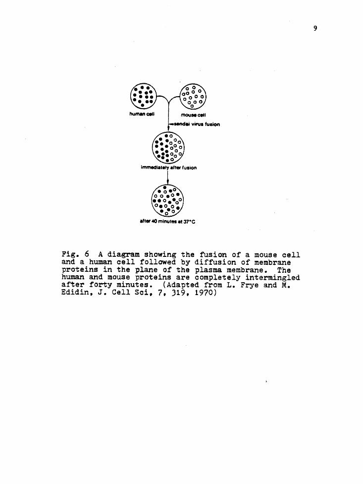
Evidence which supports this fluid-mosaic model includes
hybrid cell fusion and freeze-fracture microscopy, which will be
discussed in greater detail. The hybrid cell fusion consists of a
mouse and human cell which are fused together under the influence
of the sendai virus. By labeling specific human and mouse pro
teins it is found that the proteins become completely intermixed
with time (see Figure 6). Furthermore, this intermixing is not
observed if the fusion is performed at temperatures below 15°C
which is the freezing temperature of the plasma membrane phospho-
1 ipids [20], which supports the fluid core hypothesis of the
model.
In freeze-fracture electron microscopy cells are frozen so
that the aqueous regions become stiff. If these frozen specimens
are then fractured the cleavage line will pass through the area
of least resistance, usually near the center of the bilayer.
immedlatety after fusion
after .-0 minutes at 37•c
Fig. 6 A diagram showing the fusion of a mouse cell and a human cell followed by diffusion of membrane proteins in the plane of the plasma membrane. The human and mouse proteins are completely intermingled after forty minutes. (Adapted from L. Frye and M. Edidin, J. Cell Sci, 7, J19, 1970)
9
10
Each protein will remain with the lipid layer to which it was
most firmly bound. Such freeze-fractured membranes,· when observed
with a scanning electron microscope, would seem to support the
fluid-mosaic model and have shown that the cytoplasmic face of
the membrane has a much larger concentration of internal proteins
than does the external face.
Since natural membranes are fragile and difficult to obtain
for in-vitro studies, research has been confined to various forms
of artificial membranes, which allows the exclusion of numerous
complicating variables associated with biological membranes.
Thus, individual chemical effects and mechanisms can be directly
investigated. Artificial membranes may be formed from both
natural and/or artificial materials, including various mono
glycerides or lecithins. Glycerylmonooleate (<1v\O) was the only
lipid employed in this study, solely for ease of comparison with
various literature values obtained from experiments which also
utilized C1vD membranes.
Electrical Properties of Membranes
Among the electrical properties of biological membranes
which have been investigated over the years are: capacitance,
conductance, resting potential, breakdown voltage, and refractive
index. Researchers [35] have shown that artificial bilayer lipid
membranes are suitable models of natural membranes since they
reasonably mimic these electrical properties of natural
membranes.

11
Two of the most straightforward properties of a BLM to
measure are conductance and capacitance. An unmodified bilayer
lipid membrane has a very small conductance, a property which can
be understood by considering the self energies of the free ions
in the surrounding aqueous solution. The stored energy of a
distribution of charge at potential V is:
W = tQV Eq-1
where Q is the total charge. If an ion is considered as a sphere
with total charge Q, then the potential is:
v = Eq-2
where €0
is the permittivity of free space, E represents the rela-
tive permittivity of the medium (substance which contains Q), and
r is equivalent to the ionic radius. Substituting Eq-2 for V in
Eq-1 yields:
w = l Q2
87r€0 r € Eq-3
The extra energy necessary for the ion to transfer from a
high dielectric medium (water, €w = 80) to the lower dielectric
membrane (EM) is:
~w] Eq-4
It is apparent that the additional energy needed is inversely
proportional to the radius and AE so that the smaller ions comnon

12
to aqueous salt solutions (such as H+, OH-, K+, c1-) will be
unlikely to penetrate a membrane which can be thought of as
having an E in hydrocarbon of approximately 2. Using EM= 2.1
[6], Ew = 80.1, r = 1.33 A [51], Q =electronic charge in Eq-4
yields a ~W of 2.5 ev for the potassium ion. This is one hundred
times larger than the available room temperature thermal energy
of kT = 0.025 ev. The conductance is not actually zero due to
the statistical variation of self energies in a population of
ions (so that some ions will possess sufficient energy to allow
thermal penetration of the membrane) and the fact that the free
energy (amount of energy available to perform work) is also
affected by membrane structural fluctuations and surface
electrical potential. This electrical potential may result from
either the presence of a net surface charge (i.e., the charged
lipid head groups, such as phosphate or choline, or adsorbed
charged molecules) or from a net dipole moment resulting from the
orientation of polar groups (e.g. the ester linkages of
cholesterol) or amphoteric groups (as in phosphatidyl choline)
at the membrane surface. This surface potential contributes to
the free energy of the ionic species depending on the sign and
magnitude of the potential, e.g. a posftive surface potential
would be expected to reduce the penetrability of positive ions
while enhancing the penetration of negative ionic species, etc.
However, most biological membranes are negatively charged at
physiological pH's and yet permit anion exchange, thereby implying
that other transport mechanisms are involved. Those effects due
to a surface charge layer may be differentiated from those due to

13
a layer of oriented dipoles since only the former would be expected
to change in magnitude with variations of the aqueous salt concen
tration.
Membrane Modifiers
A variety of substances exist which, when added to the
membrane or aqueous environment, will cause order of magnitude
changes in the membrane conductance. Certain of these substances
(e.g. nonactin, valinomycin) function as ionic carriers and
directly affect the membrane conductance (see below for details)
while others function indirectly as modifiers which may cause
changes in membrane thickness, diffusion constants (see the
Carrier Model in Theory section), surface dipole moments, etc.,
but do not form ion complexes. In this experiment valinomycin
was employed so that convenient comparisons might be made with
various literature values.
Valinomycin and Other Ion Carriers
While searching for specific ion carriers to explain the
ablllty of some membranes to selectively transport a particular
substance against its concentration gradient (so called active
transport or "pump" action), it was discovered that valinomycin
and certain other antibiotics enhanced cation transport across
mitochondrial membranes (39]. These antibiotics were termed
ionophores because of their selective enhancement of cations in
general, e.g. K+, Rb+, cs+. The mitochondrial membrane normally
doesn't transport K+ but will in the presence of an ionophore.

14
This destroys any existing K+ gradient and leads to a new ionic
equilibrium distribution. The membrane potential due to this
ionic distribution may be obtained from the Nernst Equation [26]:
= RT
-F-ln [K+] outside
(K+] inside Eq-5
where R is the universal gas constant, T the temperature (°K) and
F is the Faraday constant. Mitchell and others, using methods
based on this, have reported values for the mitochondrial
membrane of -150 to -200 mV, "inside" (cytoplasm) negative [33].
Valinomycin has also been examined as a potential anti-
biotic. Although bactericidal, it exhibits little selectivity
and i s con s e q u en t l y no t us e f u l i n med i ca l t he r a p y • Howe v e r , i t
has continued to be an important research tool for investigating
ion transport functions in artificial membranes [9,28,45,46,47,
48,50].
The ability of valinomycin to transport cations can be
explained by its hydrophobic exterior and hydrophilic interior
(see Figure 7). This allows the carriers to insert themselves
into a membrane while providing carbonyl groups to coordinate
with the inorganic cation, thereby providing a clathrate haven
permitting safe transport through the membrane [18].

N
0
Fig. 7 Structur~ of Valinomycin
M = Metal Ion A = L-lactate B = L-valine C = D - hydroxytsovalerate D = · D- valine
15

16
Carrier-Ion Complexes
Although valinomycin is primarily known as a carrier of
potassium, it will also transport other cations of the same
chemical family (but not lithium, presumably because lithium's
larger sphere of hydration prevents adequate complexing with the
carrier). In order to make comparisons among the various exper-
imental methods, this study has been restricted to the widely
employed ions K+ and Rb+. There are several factors which
indicate that rubidium may be the ion of choice.
First, consider the general reaction of a metal cation (M+)
with a carrier
Valinomycin + M+ "'"".....,. Valinomycin - M+ complex
where the equilibrium constant, in water, is defined by:
K =
~S' CS'~ signify the equilibrium concentrations, in bulk
aqueous solution, of the carrier-ion complex, carrier and cation
respectively. Rubidium has a smaller K than does potassium (O.l
vs. 1.0 M-1 [9]). This implies that there is little complexing
between valinomycin and rubidium in water (i.e. ~S is small).
Therefore, the total concentration of valinomycin in the aqueous
solution (C 0 = CS+ ~S) may be approximated by Cs if rubidium
is the cation. This approximation holds for ionic concentrations

17
less than or equal to 1.0 M (T = 25°C); at higher concentrations
the aqueous complexing is no longer negligible [9,42]. Our own
study examined concentrations ranging between lo-3 and 1.0 M so
that this approximation could be used in the calculation of the
number of carrier molecules which might be expected to enter a
membrane in contact with aqueous solutions containing the ions.
The calculated value can be given in terms of the partition coef-
f icient, ~s, which is the ratio of the carrier concentration
averaged over the volume of the membrane to the carrier con-
centration in the aqueous solution. The partition coefficient,
~s, is a dimensionless parameter which may be written [27]:
~s = Eq-7
where NS is the number of carrier molecules per membrane unit
area, d is the membrane thickness, and CS is the concentration of
the carrier in the aqueous phase. Researchers have found a
variety of ways to employ the ion carriers and the above
relationship to investigate membrane charge transport.
Experimental Approaches
Various methods have been employed to investigate the
electrical properties of bilayer membranes and the variations
which occur with the addition of modifying substances, such as
valinomycin. Of particular value in uncovering information on
the kinetics of complex formation and transport are the relaxation

18
methods. These include voltage-jump techniques, where a membrane
is subjected to a sudden displacement of the voltage and the
resulting membrane current is followed over time [8,9,47]; and
the charge-pulse technique, where a short current pulse is used
to charge the membrane capacitance to an initial voltage and the
subsequent decay of voltage is monitored after the termination
of the pulse [7]. Other studies have utilized temperature jump
experiments [24] and current noise analysis [25] to investigate
membrane electrical properties without the application of membrane
biasing external voltages. Another approach to obtain kinetic
information, suggested long ago but little used to date, involves
the application of an external voltage which varies periodically
with time (alternating current studies) and observing the
resultant variations of membrane current.
Alternating current studies have the additional advantage of
remaining sensitive to membrane capacitive changes as well as
variations in membrane conductance. Such dynamic measurements
were explored in this experiment. In particular a GVIO bilayer
membrane separating two identical aqueous salt solutions (see
Figure 8) of K+ or Rb+ with valinomycin was exposed to an alter
nating voltage. In the following section the theoretical basis
for Steady-State, Voltage-Jump, Charge-Pulse and Alternating
Current experimental approaches will be detailed.

Electrodes
/~
I I I I I I 0 I I I I I I I I I
-----------~---- ---~ ' ', ' ' ' ' ', ' l+-Cup~
Fig. 8 Tef Ion Cup and Container Basic Experimental Set-up
19

THEORY
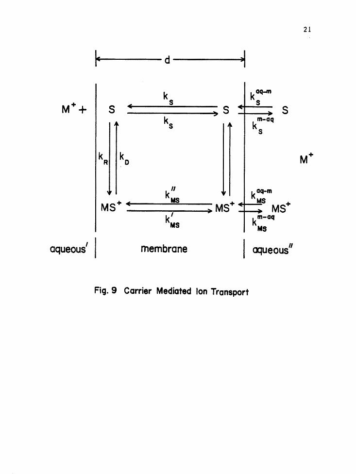
Carrier Model
A simplified model for ion transport of alkali metal ions
in aqueous solution by a carrier, such as valinomycin, may be
sunmarized by three basic steps (Figure 9): formation of the
carrier-ion complex within the membrane surface; transportation
of the complex to the opposite surface, under the application of
a voltage; and release of the ion into the solution. A detailed
analysis must take into account a number of physical processes
[45]:
(1) adsorption or release of the neutral carrier at the
membrane surface (rate constants k;q-mand k~-a~ where aq-m denotes
from aqueous to membrane, etc.);
S(aq) S(m) Eq-8
where: S =carrier, aq = aqueous solution and m - membrane;
(2) the formation or dissociation of the carrier-ion
complex (rate constants kR and kD respectively);
kR
M+(aq) + S(m) MS+(m)
where: M+ = metal ion, with aqueous concentration~ and
S =carrier, with aqueous concentration c5
;
Eq-9
21
r~--d--~~
k kaq-m
M++ s - s s s ._ s ... -
ks m-aq ks
kR ko M+
k II kaq-m + MS +- MS +
MS _c ---~-~MS ...,_ -: MS k ' km-aq
MS MS
aqueous' membrane aqueous"
Fig. 9 Carrier Mediated Ion Transport

22
(3) the adsorption or release of complexes, formed in
the aqueous solution, at the membrane surface (rate constants
kaq-m d km-aq)· MS an MS '
MS+(aq)
kaq-m MS
MS+(m) Eq-10
(4) the electrodiffusion of the complex through the
membrane interior (rate constant k~S for movement in the direc-~
tion of the applied field (E) and k~S for transport in the oppo-
site direction);
(5) and the diffusion and back diffusion of the neutral
carrier through the membrane due to concentration gradients (rate
constant, ks>·
Ionic Charge Transport
The charge transfer across the membrane interior may be
described by an "Eyring" mechanism [27] where one regards the two
interfaces (an interface refers to the poorly demarcated regions
where water and lipid intermingle on each side of the membrane)
as being separated by a synmetrical energy barrier (see Figure 10).
If an MS+ complex possesses sufficient energy it can "jump"
across this barrier and transport the charge in this fashion.
Presumably the uncomplexed carrier is also able to traverse its
own particular energy barrier.
Although the uncomplexed ion is predominantly excluded from
the membrane, S and MS+ may be exchanged between the aqueous and
membrane phases (equations 8 and 10). Besides this, a chemical

23
r ...... --- d ___ __..),
Potential Barrier
aqueous membrane aqueous
Fig. 10 Erying Mechanism Potential Barrier

24
reaction can take place at the interface between a carrier S in
the membrane and an ion M+ from the aqueous solution (equation 9).
The rate constants for these reactions may be related to the
partition coefficients of the carrier and complex, as outlined
by Lauger and Stark [27]. If we denote the concentrations of S
and MS+, in the left-hand and right-hand interfacial regions, by
t n I II ( ) NS, NS' NMS and NMS' respectively, then the fluxes ¢ of S and
MS+ across the membrane are given by:
¢s =
¢MS =
N" ) s
k" N" MS MS
Eq-11
Eq-12
The current density (J) may be related to ¢MS' as the complex is
the only charge carrier within the membrane, by (F = Faraday
constant):
J = Eq-13
In the presence of an externally applied voltage the rate
constant ks, for the translocation of the neutral carrier S,
should be the same regardless of the ionic flow's direction.
However, the rate constants k~S and k~S' associated with trans
location of the charged complex, will vary with the external
voltage V. For V = 0:
k~s = k" MS = Ae-E/RT = k
- MS Eq-14
E is the energy (per mole) for zero voltage at the top of the

25
membrane's syrnnetrical energy barrier (R = gas constant,
T = absolute temperature, A= constant). For V ~ O, the barrier
height will be changed by the electrostatic energy of the charged
complex (MS+). If one assumes that the electrical potential L(x)
in the center of the membrane (x = d/2, d = membrane thickness)
is equal to V/2, then the barrier height becomes E - FV/2 for
transport from right to left and E + FV/2 for transport from left
to right. Therefore,
= k -u/2 MSe
k" = k u/2 MS MSe
u = v RT/F Eq-15
Eq-16
It can be shown [3] that L(d/2) = V/2 is valid for a constant
field strength (i.e., a homogenous dielectric) within the membrane,
which is a good approximation for lipid bilayer membranes, under
most experimental conditions.
For each particle at each interface the sum of the net chem-
ical production (equation 9) and of the fluxes toward the interface
must vanish in the stationary state:
' dNS
dt k~-~~ = 0
Eq-17
m-aq11
0 ks NS =
Eq-18
dN~S dt
dN" MS
dt
=
= k ("_ -N" R-"M S
~MS
26
+ aq-m m-aq_. ,
kMS ~S - kMS ~MS = 0
Eq-19
m-aq kaMqS-mNM" S = + kMS ~S - 0
Eq-20
For V = O, the membrane and aqueous solution chemical processes
a r e i n e q u i 1 i b r i um , i • e • , e q u a t i on s 8 , 9 and 1 0 a r e i n d y n am i c
balance. I If I II
Then the relations NS = NS = NS' NMS = NMS = NMS'
and k~S = k~S = kMS w i 1 I ho 1 d and the f o I I ow i n g re 1 a t i on s may
be obtained from equations 17 - 20:
- kR~NS + kDNMS = 0 Eq-21
aq-m m-aq 0 Eq-22 ks cs ks NS =
m-a~ aq-m kMS S kMS NMS = 0 Eq-23
From equations 22, 23 and 7, the equilibrium state may be charac-
terized by the partition coefficients of the free carrier and
complex, Ys and yMS respectively.
2N 5 /d 2kaq-m
Y5 = = s
cs dk 5 Eq-24
2NMS/d 2kaq-m MS
YMS = = CMS
dkm-aq MS Eq-25

27
In addition, the equilibrium constant of the chemical reaction
(Kh) may be expressed in terms of Ys and yMS by using equations
21, 24 and 25.
= = = K =
Eq-26
In principle, both reactions (equations 9 and 10) could be
the controlling or rate limiting processes for the charge
transport through the membrane interface in the presence of an
external voltage. However, due to the hydrophobic exterior of
the carrier, ~S and c5 in the aqueous solution will be quite
small. The ratio of c5 lipid to CS aqueous has been determined
to be about 5xl0 3 [48] for monactiR, a carrier similar to valino-
mycin. Since ~Sand c5 are small, the carrier is predominantly
available as a substrate only within the membrane. Therefore,
the rate of the chemical reaction (equation 9) should be high
when compared to the rates of the exchange reactions (equations
8 and 10), and the bulk of the charge transport through the
interface will occur via the chemical reaction [27,45].
In order to investigate the validity of this model, attempts
have been made to determine the values of the various rate constants.
Experimental approaches in the past have included voltage-jump,
charge-pulse, current noise analysis, and steady-state methods.
This paper employs alternating current methods, which will be
developed following a brief discussion of voltage-jump,
charge-pulse, and steady-state theory.
28
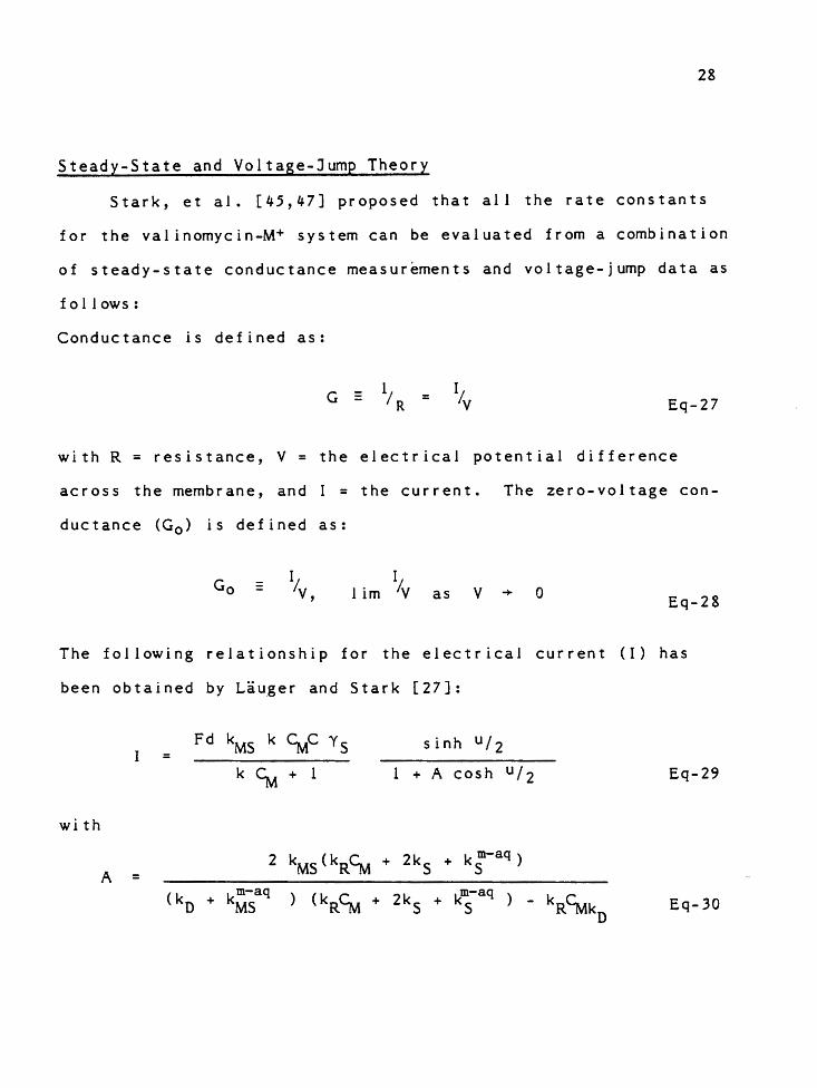
Steady-State and Voltage-Jump Theory
Stark, et al. [45,47] proposed that all the rate constants
for the valinomycin-M+ system can be evaluated from a combination
of steady-state conductance measurements and voltage-jump data as
follows:
Conductance is defined as:
G - = Eq-27
with R = resistance, V = the electrical potential difference
across the membrane, and I = the current. The zero-voltage con-
ductance (G 0 ) is defined as:
as v -+ 0 Eq-28
The following relationship for the electrical current (I) has
been obtained by Liuger and Stark [27]:
Fd kMS k ~c Y5 sinh U/2 =
k~ + 1 1 + A cosh U/2 Eq-29
with
2 kMS(kR~ + 2ks + k5-aq) A =
(ko + m-aq ) (kR~ + 2kS +
m-aq ) kR~k kMS l<S -D
Eq-30

29
Ev a l u a t i n g E q - 2 9 i n t he l i mi t o f sma l l v o l t age s ( u + 0 ) and
substituting for I in Eq-28 yields:
2 F dkMS
2RT ( k~ + 1 ) ( -1 + A) Eq-31
From equations 6 and 7
d Ys Co =
2 l + ~k Eq-32
where
Since k << lM-1 for the carrier-ion complex, then it follows that
~k << 1, which in turn implies that the concentration of valino
mycin in the membrane, NS' is independent of the ionic species
concentration, i.e.:
d -1 N5 ~ 2 Y
5c 0 , for k << lM Eq-33
Substituting from equations 26 and 33 into equation 31 gives:
= Eq-34
Furthermore, for ~k << 1 and Eq-33, Eq-34 reduces to:
Eq-35

30
If one can neglect the ionic transport due to the exchange reac
tion (equation 10), which is reasonable for valinomycin (see
above discussion of Ionic Charge Transport), then Eq-30 may be
evaluated as if km-aq << kRCM + 2k5 and km-aq << k0 ; in which
case A reduces to:
A = +
Eq-36
Finally, combining equations 27, 29 and 31 leads to an expression
for G/G0 which depends only on A and u •
2 u
. h U/2 ( 1 + A) __ s_1_n ___ ~--l + A cosh U/2 Eq-37
G and G0 can be measured experimentally as a function of u and
the corresponding A's calculated using Eq-37. By doing these
studies at different ionic concentrations, CM' a graph of A vs ~
(equation 36) can be prepared and the ratios 2kM5 /k0
(y intercept)
and kRkM5 /k0 k5 (slope) extracted (see Figure 11). In addition,
Eq-35 yields y5kM5 /k0
so that three independent equations com-
b i n i n g t he f i v e. v a r i ab 1 e s ( y 5 , kMS , k 5 , kR and k 0 ) can be de d u c e d
from steady-state conductance measurements.
Further information obtained from membrane relaxation data
can now be used to complete the solution. In voltage jump experi-
ments a short voltage step is applied and the resulting current
discharge is measured as a function of time. This current can be
represented by the sunmation of two decay curves [47]:

A
k k slope= R Ms
k k D S
31
Fig. I I Parameter Determination through Variations of A vs Cm

32
I ( t) = Eq-38
where the a•s (relaxation amplitudes) and T's (relaxation time
constants) are related to the rate constants kMS' k5 , kR and
kn by the following equations [47]:
l + P(~kR + 2k5 ) + ~kRkn
2 2(~kR + 2k 5 ) is-Eq-39
T 1 = l/Q - /s- Eq-40
p - 1 (~kR - kn + 2k5 - 2kMS) 2 Eq-41
Q - 1 (~kR + kn + 2ks + 2kMS) 2 Eq-42
s - p2 + ~kRkn Eq-43
Experimental determination of these a•s and T's from graphs of
I vs t on log-log scale along with the steady-state information
are therefore sufficient to allow an exact numerical solution for
each of the rate constants. The most significant problem with
this experimental approach is that the time resolution is limited
by the charging time of the membrane (TC). Usually membrane
resistance is much greater than the external resistance Re
(Re= R5+R1, R5 = resistance of solution and electrodes, Ri=
input resistance of the amplifier) so that TC~ ReC = (R5+Ri)C

33
where C is the combined electrical capacitance of the membrane
(~) and septum (Cs>. If Ri can be kept on the order of Rs then
LC as low as 0.2 µsec can theoretically be achieved [28]. The
a c tu a l LC i s us u a l l y approx i mate l y ten t i mes th i s val u e ( ~ 2 µsec )
since the charging current needs to decline to a small fraction
of the initial value before the low amplitude relaxation currents
can be measured. In addition, noise in the electronic measuring
circuit may overlap and obscure the relaxation currents.
Charge-Pulse Theory
One method which circumvents the RC time limitation of the
voltage-jump experiments is the charge-pulse technique. At time
t=~ the membrane capacitance is charged, virtually instantaneously,
0 to a voltage VM. Then the external circuit is switched to a virtu-
ally infinite resistance and the subsequent voltage decay monitored.
The rate of change of the concentrations of S and MS+ at the
right and left interfacial regions, after the charge pulse, is
given by [7]:
d N' kR~N~ kDN~S k (N'-N") s = - + -
dt s s s Eq-44
d N" k ~N" kDN~S k (N"-N') s = - + -
dt R S s s s Eq-45
' d NMS = kR~N~ - kDN~S k~SN~S + k~SN~S dt Eq-46
d N" k ~N" kDN~S k" N" ' ' MS = - + kMSNMS dt R S MS MS Eq-47

3 4
The decay rate of the voltage VM is a function of both the
specific membrane capacitance~ and the current density, J, in
the membrane:
~ dt
= = (k ' N" k" N" ) MS MS - MS MS Eq-48
k~S and k~S are both voltage dependent and functions of time
(see Eq-15 and Eq-16). If the analysis is further restricted to
sma l 1 v o 1 tag es ( I u I < < l or IV M I < < 2 5 mV ) then the f o l l ow i n g
approximations can be used:
Eq-49
Eq-50
Equations 44-48 constitute a system of five linear differen-
tial equations from which, in the case of small voltages, VM(t)
may be obtained (see [7, appendix A] for details), in the
f o 1 1 ow i n g f o rm :
= + +
Eq-51
Eq-52
l a.i and Ti= /A.i (i = 1,2,3) are the relaxation amplitudes and
relaxation times respectively. These a.•s and T's may be

35
expressed in terms of the rate constants but the resulting
equations are quite cumbersome. A more convenient formalism
involves the following quantities:
pl = A.1 + A.2 + A.3 Eq-53
p2 = /q A. 2 + A.1A.3 A.2A.3 Eq-54
P3 = A.1A.2A.3 Eq-55
P4 = a1A.1 + a2A.2 + a3A.3 Eq-56
P5 = a1A.i + a2A.~ + a3A.~ Eq-57
From these five variables, which may be experimentally determined
from the a's and L's, the four rate constants kR' k0 , ks and kMS
as well as the carrier concentration N0 (N 0 = N~+N;+N~s+N~S} may
be calculated (see [7, Appendix A]}:
Eq-58
ko = 1 [ plp5 - p2 + P3 -(:m 2kMS P4 P4 Eq-59
ks 1 P3
= 2k
0 p4 Eq-60
kR = l (Pl- P4- 2ks- 2kMS- ko) ~ Eq-61
No = 2RT ~ p4 (1 + ~)
F2 kMS ~kR Eq-62

36
This method has an additional advantage in that very small
applied voltages may be employed. However, both the experimental
procedure and subsequent calculations are more complicated plus;
any voltage dependence of the rate constants cannot be determined
in this manner.
A.C. Theory
In both the voltage-jump and charge-pulse experimental
methods a step change was applied to the membrane system.
Information about the transport kinetics of carrier-mediated ion
transport, in principle, can also be extracted from the applica-
tion of periodic perturbations to the system. Such a harmonically
oscillating voltage may be represented by:
= VO COS Wt M Eq-63
The response of the membrane may then be measured for various fre-
quencies w. In the steady state the current ls also given by a
harmonic function, with the same frequency w:
I(t) = I 0 cos Cwt -¢> Eq-64
where I 0 ls the current amplitude and ¢, the phase shift, may be
expressed by the (small-signal) admittance Y(W).
= = V~ "1Re2 [Y(W)] + Im2 [Y(W)] Eq-65
tan¢ = - Im[Y(W)] I Re[Y(W)] Eq-66
where Re means "the real part of" and Im "the imaginary part of."

37
At any given instant the current I in the membrane is the sum of
the charging current r__~ dVM and the current due to charge move~ cit
ments within the membrane.
As in the charge-pulse method, equations 44-47 represent the
interfacial concentration variations of S and MS+, with time.
Now, however, k~S and k~S must be represented by periodic func
tions of time, so equations 49 and 50 are replaced by:
k~5 ~ ~s [1 + ~o cos Cwt~ Eq-67
Eq-68
The solution of equations 44-47 may now be obtalned by standard
differential methods [17,25]. The results are (e 0 = elementary
e l e c t r on i c ch a r g e , '\, = mem b r an e a r ea , k = t h e Bo l t zma n n con s t an t ,
and ~ = memb r an e cap a c i tan c e ) :
~(w) e2
- Re[Y(w)] = 0
kT
Eq-69
Eq-70

38
with
kMS la- p ~s p + ;a Ct 1 = a. 2 = ;a- • ;a-+ Q ;a Q - ;a
Eq-71
and
1 1 1'1 = Q + ;a- 1'2 = Q ;a -
Eq-72
where
p = 1 (CMkR - kn + 2ks - 2kMS) 2 Eq-73
Eq-74
Eq-75
The real part of the admittance (Eq-69) corresponds to the
membrane conductance, while the time constants T1 and T2 (Eq-72)
are identical to the relaxation times for the voltage-jump
experiments.
Kolb and Lauger used a similar analysis in their current
noise experiments [25]. They employed the Nyquist theorem (an
equation relating the voltage fluctuations in linear electrical
systems with the electrical resistance [12,34] to describe the
spectral intensity, SI; at equilibrium, V=O, as:
SI (w) = 4kT • Re[Y(w)] Eq-76

39
The spectral intensity represents the power within a frequency
range dw, for a particular w, which is being dissipated as noise.
Substituting Eq-69 into Eq~76 gives a current noise spectral
intensity of:
=
Eq-77
It can be seen from Eq-46 that the spectral intensity becomes fre-
quency independent at both high and low frequencies. Furthermore,
S1(o) is related to the membrane steady-state conductance, while
S 1 ( 00) is related to the initial membrane conductance which is
observed inmediately after the application of a voltage jump. By
simultaneous solution of equations 71-75 and 77, the following
expressions are obtained for the rate constants(A1 = l/T1,
ks
kR
ko
=
=
=
=
1 2
A.1A.2 {4k~s (l-a1-a2)}
4kMS (a1A.t + a1A.~ - 4k~5 )
a1a2 A.1A.2 (A.1-A.2) 2
2CMkMS (A.1A.t + A.1A.~ - 4k~ 8 )
a2A.~ + a1A.f - 4k~S
2kMS
Eq-78
Eq-79
Eq-80
Eq-81
Eq-82

These equations 1 are then used to determine the rate constants
from the experimentally measured a's and r•s.
1 It should be noted that equations 78-82 do not correspond exactly to equations Bl-B5 in [25]. Several transcriptional and/or printing errors appeared in the original publication. Equations 78-82 do correctly invert to equations 69-75.
40

EXPERIMENTAL METHODS AND ~TERIALS
Introduction
The basic experimental setup consists of a membrane formed
across a hole in a septated teflon cell separating two identical
aqueous ionic solutions and an accompanying electrical circuit to
measure and apply the current and voltage across the membrane.
These basic components are diagranmed in Figure 8. The materials,
membrane forming technique, and electrical circuits will be
discussed in detail.

42
Materials
Bilayer lipid membranes were formed from a solution of gly
cerylmonooleate (GAO) in n-decane. The CMO was purchased from
Nu-Check-Prep, Inc. (> 99% purity). The CMO was stored as a 5%
weight by volume stock solution (1,000 mg solute in 1.0 ml solvent
is equivalent to a 100% solution) in chloroform at -15°C. Membrane
forming solutions were mixed daily by removing, at room temperature
the chloroform from a known volume of stock solution (measured by
a Rainin micropipet) in a rotary evaporator for fifteen minutes at
-30 in Hg vacuum and adding n-decane to achieve the desired
concentration (usually 2.5%, weight by volume).
Aqueous solutions containing the metal ions were formed from
KCl or RbCl (> 99% pure, from Matheson, Coleman and Bell) with
water deionized through a Q2 Millipore system (resistivity > !OM
-cm). Ionic strength was maintained at 1.0 M through the addi
tion of appropriate amounts of LiCl to any of the aqueous solu
tions where the concentration of metal ion was less than one
molar. This was necessary to insure a constant membrane surface
potential so that any observed variations in the rate constants
with different ionic concentrations could not be ascribed to
variations in the aqueous charge distribution. In addition, the
lM concentration keeps cell resistance low and improves the
accuracy. Lithium has a negligible effect on membrane conductiv
ity in the presence of valinomycin [4,32]. The lithium presumably
acts as an inert electrolyte which cannot coordinate with the
valinomycin because of its very large sphere of hydration.

43
The addition of LiCl is also of importance in the d.c.
measurements. Here the additional ions lower the resistance of
the solution (RE = electrical resistance, Rs = resistance of the
aqueous solution, ~ = membrane resistance) and insure that
Rs does not overwhelm RE and ~ as the concentration of the
transport ion decreases to 0.001 M. The aqueous solution pH was
consistently between 6 and 7.
Valinomycin (A grade, from Calbiochem) was stored as a stock
solution with ethanol and kept refrigerated, in a dark bottle
wrapped with foil. This stock solution is added to the aqueous
ion solution prior to the formation of membranes. The ethanol
concentration in the aqueous solution was approximately 0.08% and
should not have affected the structural or electrical properties
of the bilayers [45]. It is also possible to add the valinomycin
directly to the membrane forming solution (10- 7 M aqueous is
-3 equivalent to 10 M membrane [45]). This technique was tried but
problems were encountered with membrane structural stability. The
membranes would last only from three to ten minutes. This should
not have been due to ethanolic disruption as the ethanol was
removed, along with the chloroform, in the rotary evaporator at
-30 in Hg vacuum for 45 minutes. This method was not pursued
further, although it has the inherent advantage of a shorter
conductance stabilization period.

44
Cell Preparation
Both the a.c. and d.c. teflon cells were initially baked for
six days at a temperature between 90° and 130° C, then soaked in
chromic acid and finally boiled in NaOH/EtOH to remove any
possible nonactin contamination from prior experiments, as
reported by Smejtek and Paulis-lllangasekare [44]. In between
uses the cells were stored in 95% EtOH. Prior to use the cell was
rinsed with fresh ethanol and force dried by a Sanyei E-2105 hair
dryer operating at 1200 watts for 10 to 15 minutes. Whenever new
ionic concentrations or ions were to be investigated a more thorough
cleaning procedure was followed by boiling in a 95% EtOH/NaOH
solution for ten minutes followed by ten minutes of boiling in
distilled water.
After any boiling procedure the cell was "painted" prior to
forming any membranes. After drying the cell the painting was
performed by placing the aperture in a nitrogen gas stream and
applying a brush of lipid around the hole. The lipid was spread
evenly, moving away from the center in a spiral fashion. This was
performed with three brush fulls of lipid until a uniformly
smooth, glistening layer was present. It was found that the form
ation ease and membrane stability was enhanced by this painting
procedure. Then the cell was placed in an acrylic container, the
aqueous ion solution added, and membranes formed as follows.

45
Membrane Formation
Membranes were formed by drawing a sable brush dipped in
lipid across a circular aperture in the wall of a teflon cell.
Inmediately after formation the membrane is thousands of angstroms
thick, but within seconds the central portion begins to thin and
continues until a thickness of approximately 70 ~ is reached.
This thinning process begins at the bottom of the membrane and
progresses upward. The excess lipid gathers on the cell surface
and in an annular ring within the hole's rim, surrounding the
optically black, thin membrane. This ring is referred to as the
torus (see Figure 12). Only the black portion contains the
bilayer configuration which corresponds to biological membranes,
so it is important to insure that sufficient time is allowed for
its completion. In order to minimize the torus size and lipid
build-up, as little membrane solution as possible was used. This
also reduces any exchange of valinomycin that might occur between
the black membrane and surrounding lipid.
Electrical Measurements
The basic alternating current and direct current circuits and
their respective operational procedures will now be discussed in
detail.
Alternating Current System
The alternating current measuring system includes the
following components (see Figure 13):

~---i.----1--- Lipid on the Teflon
~~r--r---r-- Rim of Teflon Aperture
~iill----4-------1--- Bilayer Membrane Area
Torus (cross hatched)
Fig. 12 Membrane Formation on the Teflon Cup
46

Dat
a (G
e, C
c)
Mic
rop
roce
sso
r
Co
ntr
ol
Lin
es
Au
tom
ati
c B
alan
cing
B
ridg
e
r'\
_I
Mem
bran
e C
el I
Uni
t
Fig
. 13
A
.C.
Inst
rum
enta
tion
Dat
a (F
req
)
Fre
quen
cy
Gen
erat
or
"J
Fre
q 1
.-i -----?~~
Cou
nter
rv
Mic
rosc
op
e
-I==' .......

48
(1) A Hewlett-Packard 4270A automatic capacitance bridge,
which is used to measure the conductance and capacitance of the
cell-membrane system. The standard instrument has been modified
by A.O. Pickar to allow operation with an external oscillator,
thereby providing measurements over a continuous frequency range
and at low test voltages.
(2) A Hewlett-Packard 5245L Electronic Counter to record the
frequency being applied to the membrane.
(3) Two oscillators: one contained within the microcomputer
which automatically generates the experimental frequencies; the
other, a Hewlett-Packard HP-651B test oscillator, is used as an
external source to perform manual comparisons with the automatic
oscillator.
(4) A relay box containing various resistances and capaci
tances, which is used to modify the membrane circuit (see A.C.
Operations}.
(5) An amplification unit to boost the signal and filter
noise from the frequencies produced by the signal generating
components within the microcomputer.
(6) A Motorola MEK6800D2 microprocessor chip interfaced with
various memory, control and frequency chips performs an automatic
sequential run of twenty-five frequency steps (0.1 to 900 KHz} and
stores the measured conductance, capacitance and frequency values
for each step.

49
Microcomputer
The signal generating board consists of two frequency chips;
one with a range of 0.123 to 400.0 KHz, the other with two distinct
ranges {lower range from 200 to 400 KHz, and a higher range of 500
to 1,000 KHz). Since the frequency range of the two chips overlaps
between 200 and 400 KHz, it was necessary to decide which frequency
chip would be used for that range.
To accomplish this a dumny circuit was designed to simulate
the conductance and capacitance of a G\AO membrane in the presence
of val inomycin {~ = lOnF, G0 = 100 µS). The microcomputer then
performed an automated run on this dumny membrane circuit. The
test oscillator was then used to generate identical frequencies,
and the corresponding conductance and capacitance values were then
compared with those obtained by the microprocessor. The greatest
discrepancy occurred at higher frequencies {> 300 KHz), but even
then the capacitance and conductance values for the automatic and
manual runs agreed within one percent. An oscilloscope was also
used to monitor the wave forms produced by the microprocessor.
The low frequency range chip generated well-formed sinusoidal
waves except for slight distortion of the peaks (between 0.1
and 0.5 KHz) and gross assymetries of frequencies greater than
300 KHz. The high frequency range chip wave forms were good
except for definite peak flattening of the 200 KHz wave generated
by the low range of this chip. From these considerations the
following assignments were made: low frequency chip generated
0.1 - 200 KHz frequencies, while the high frequency chip produced

50
those frequencies between 300 and 1,000 KHz (300 and 400 KHz by the
low range of the high frequency chip; 500, 700 and 900 KHz by the
high range of the high frequency chip). Progranming instructions
were loaded into the microprocessor, from a magnetic tape, using a
Sankyo SAV-1060 recorder. Data stored in the microprocessor was
output to a teletype and a paper punch tape created.
A.C. Operations
A membrane was formed (see Membrane Formation section below
for full details) across a 1.652 mn diameter aperture, in the
presence of a 1 KHz test signal. Conductance and capacitance were
then monitored by the Hewlett-Packard bridge until fluctuations in
both values had stopped (approximately five to ten minutes after
formation)~ Then an area measurement was made of the bilayer por
tion of the membrane as follows: an American Optical fibre optics
system with two independently flexible heads was used to illuminate
the membrane, causing the line separating the thicker torus from
the bilayer portion to glisten (see Figure 12). A measurement of
the diameter was made with a traveling microscope. The bilayer
region was assumed to be round and the area calculated from a
measured diameter. The microcomputer then was instructed to
generate twenty-five successive frequencies (O.l to 900 KHz) and
store the capacitance, conductance and frequency values for each
frequency step.
Cell temperatures were not rigidly controlled but experiments
were performed at ambient room temperature, which varied from

51
19.6° to 21.8°C. This temperature range was far from the 10°C
where substantial rate constant variations have been observed [7].
Bridge Settings
The Hewlett-Packard bridge was originally designed to operate
at four separate frequencies (1, 10, 100 and 1,000 KHz) with a
separate internal signal generating circuit for each frequency.
After modifying the bridge to accept an external frequency source,
it is necessary to select the appropriate bridge frequency range
position for the various input signals. Table 1 lists the fre
quency range which the microcomputer directed the bridge to use
for the various external frequencies. These and the other
settings listed were chosen so as to give the fewest possible
overranges and the best agreement of capacitance and conductance
values for the dunmy circuit (as described in the Microcomputer
section). The l MHz position could not be used, even for the
highest frequencies (700, 900 KHz), because of erroneously low
conductance measurements at this setting. The bridge can still
balance for these higher frequencies in the 100 KHz position, and
there is good agreement of the conductance values. However, the
capacitance measurements for these frequencies is poorer at the
100 KHz versus the 1 MHz setting. The importance of this trade-off
will be further explored in the Data Analysis section.
The test voltage position is critical in these experiments as
it determines the magnitude of the voltage applied to the membrane.
This switch must be set in either Low or Remote, as the Normal

52
position results in a five times greater applied voltage which
causes membrane instability and structural breakdown. For the Low
setting the applied voltages, to the membrane, were about 30 mV rms
for the entire run (though slightly higher for lower frequencies)
with a d.c. component of approximately 4 mV due to electrode
polarization (platinized platinum strip electrodes were used).
Table 1 - Hewlett-Packard Bridge Settings
Freq - Remote Meas Rate - Med Meas a<T - Float
Range Mode - Hold Loss Meas - G Range Step - nF (three decimal places)
Test Voltage - Low Bias Range - Off Bias Vernier - Remote
External Freguenc~ ( f) Bridge Freguency Range Position
0 < f < l 1 KHz
~ f < 50 10 KHz
50 < f < 1,000 100 KHz
After the first twenty steps (ending with 300 KHz) are
comp l et e d , a 5 l . 1 n res i s tor i s added i n s er i es w i th the c e l l
resistance and data obtained for 200, 300, 500, 700 and 900 KHz.
This procedure is also under microprocessor control so that the
change may be affected without any break in the experiment. Such
a modification is necessary because the membrane conductance becomes
so large at the higher frequencies that the bridge overranges. The
additional series resistance lowers the net equivalent parallel

53
conductance (G = l/R) of the membrane circuit, thereby eliminating
the overranges. This factor is taken into account during the
reduction of data.
The entire automated run was approximately forty-five seconds
in duration. This permitted multiple data runs on each membrane
as well as the investigation of unstable membranes with short
life spans.
D.C. Circuit Components
The d.c. circuit consisted of the following:
(1) Keithley Picoarrmeter to measure membrane current;
(2) Keithley 160B digital voltmeter;
(3) a potentiometer circuit to apply the voltage;
(4) a Hewlett-Packard Moseley 7035A X-Y recorder.
D.C. Operations
The membrane was formed across a 2.064 l1TTl diameter opening,
in the presence of a 10 mV applied test voltage. After formation
the X-Y recorder was monitored until the membrane current was seen
to have reached a steady-state value (:::::::5-15 min). Then an area
determination was made, as in the a.c. section. Finally, membrane
current values were obtained for applied voltages of 25, 50, 75
and 100 mV. The membrane usually broke if it was subjected to
voltages much greater than 100 mV.
The calomel fiber tip electrodes were stored in concentrated
KCl and rinsed with deionized water before and after use. They

54
were checked periodically for polarization by monitoring the con
ductance of a membrane without any applied voltage. No significant
polarization curents were ever observed (I ::=l0- 2 amps) so no
correction was applied to the data. All measurements were made
at ambient room temperature levels (19.6° - 21.8°C).

55
Data Reduction - Introduction
Table 2 contains a sunmary of the computer programs employed
in the data analysis. Each will receive detailed discussion
-below. Sample print-outs for certain programs are contained in
Appendix A.
Name
RE nu 1
REnU 2
TOTAL
TOECAP
PnA l
ADP 1
ADP 2
Table 2 - Computer Program Sunmary (see text for details)
Input Output
Ge( w), cc< w) Rs, ~<w>, ~(w)
GC( w), cc< w) Normalized ~( w)' ~(w)
Normalized ~(w) a.1,a. 2 ' T 1)1' 2
Normalized ~(w) a.1,a. 2 ' 't 1)1' 2
a. l,a. 2 , T l)r 2 kR' kn, ks, kMS, Ys
measured AivI ~ corrected for bulging low frequency ~ ~ ~(w) high frequency (w)
kR' kn, ks, kMS' Ys Ci. 1,0. 2 , T 1.) T 2
1M' membrane thickness ~(w)' ~(w)
~: kn, CI
ks, kMS' Ys ~(w)' ~(w)

56
REDU 1
In order to determine the various rate constants, using
Equations 78-81, values for a1, a2, Ll and L2 must be obtained from
the experimental data. This can be accomplished from a knowledge
of the membrane capacitance (CMw) and conductance (~W} for various
applied frequencies, as will be detailed in the following pages.
However, the Hewlett-Packard bridge measures GC(w) and CC(w)
which transforms to the following equivalent membrane series cicuit,
where x
R

57
The REDU 1 program evaluates Rand Rs (the cell resistance)
from which ~may be calculated, as above. Then the membrane
conductance and capacitance are obtained from
x/w = =
)
Appendix A contains an example of the REDU 1 experimental data
printout, which shows the bridge readings GC(w), CC(w) followed by
cell resistance computations and finally, the calculated ~(w) and
~(w) values. The conductances clearly indicate the increasing
influence of RS with the higher applied frequencies. A detailed
discussion of the actual RS determination follows.

58
Determination of Cell Resistance, R5
The cell resistance can be graphically determined for each
membrane data run by plotting CC vs GC' for successive applied
high frequencies, and then extrapolating the curve as a semi-
circle to obtain the cell impedance at infinite frequency {see
Figure 14 and Table 3). This method takes advantage of the fact
that at high frequencies the membrane/cell system behaves as a
practically pure capacitance in series with the cell resistance.
For such a circuit the admittance of the system falls on a semi
circle when plotted in the complex plane [16]. The intercept of
this semi-circle with the zero-susceptance axis corresponds to the
conductance due to the application of an infinite frequency. The
i·nverse of this conductance is then taken to be the cell resistance.
This graphical procedure is carried out analytically in REDU l for
several sets of frequences as follows:
{l) wee and GC for two successive frequencies {e.g. frequency
steps 25 and 24 in Table 3) are assumed to be points on the
s em i - c i r c l e ;
{2) a perpendicular bisector is constructed between the two
points and its intersection with the x-axis is used to identify
the center of the circle which, in turn, allows a determination of
the radius {r);
{3) the r determined in step {2) is then used to construct a
semi-circle which includes the points from step {l);

7 6 """"
'""' ~ ~5
<..>
3 ~4
<..>
z <( ~
3 w
<..>
C
l)
~2 I 0
B
0
01
00
0 7
0 K
Hz
Mem
bran
e /M
ea
suri
ng
-eel
I S
yste
m
rG,C
-i
----
0 -
---
----
30
0
-.....
..........
.... -
.....
,...,,
.. ,,.
02
00
''Q
...5
00 K
Hz
,,.,,.
', ', '
cm
''<\ 7
00
\
\ \ \ \ ~I
MH
z \ \ \ ' '
I ~~L_~~·~~~·~
8 t
' '
' I/
Ro
2 3
4 5
6 C
ON
DU
CT
AN
CE
, G
(m
D,-
1)
7
Fig
. 14
G
raph
ical
D
eter
min
atio
n o
f C
ell
Res
ista
nce
Vt
\0

60
(4) the high frequency intersection of this semi-circle with
the zero-susceptance axis is taken to be the conductance due to
the cell resistance (in the limit of high frequency RS should be
the dominant circuit component, as described above) and R~ is
calculated from the inverse of this conductance;
(5) steps (1) to (4) above are then repeated for the next
couplet of frequencies (e.g. frequency steps 24 and 23 in Table 3);
' (6) the two Rs values obtained in steps (1) to (5) are then
averaged to yield Rs ; avg
(7) since RS includes the 51.10 resistance added in avg
series with the cell resistance to prevent bridge overranges (see
A.C. Operations) the actual cell resistance is calcluated from
Rsavg by, Rs = Rsavg - 51.l;
(8) steps (1) to (7) are repeated for two more triplets of
frequencies (frequency steps 24, 23, 22 and 23, 22, 21 in Table 3).
Steps (1) to (8) above result in three values for Rs which are not
identical. Due to slight distortions present in the microprocessor
generated wave forms at frequency steps 21 and 25 (200 and 900 KHz)
the value calculated from the frequency triplet 24, 23, 22 was
generally used in subsequent calculations as the assumed cell
resistance.

61
Table 3 - Typical Cell Resistance Calculation
(see text for details)
Freq Freq cc GC RS, RS avg Rs<Rs -51.1) avg Step (KHz) (pF) (µS) (Q) (Q) (r2)
25 884 750 5,880 > 168.8
24 693 932 5,850 > 168.4 117.3 > 168.l
23 496 1,270 5,710
24 693 932 5,850 > 167.0
23 496 1,270 5,710 > 166.8 115.7 > 166.5
22 295 1,924 5,134
23 496 1,270 5,710 > 165.6
22 295 1,924 5,134 > 166.1 115.0 > 166.5
21 204 2,375 4,603
Data obtained for a QviO membrane separating an aqueous solution
(0.1 M RbCL, 1.0 M LICl, l0-7 M valinomycin) (RVCM 6).

62
RE.DU 2, TOTAL, TOECAP
The calculated ~(w) and <\,\(w) data values can now be normalized
and the curve fit to extract the desired parameters (a's and ~'s).
REDU 2 performs the normalization while TOECAP and TOTAL curve fit
the normalized capacitance and conductance data respectively. A'
discussion of the normalization process follows. First, consider Eq-69:
2 [ eo ~ ( w) :: Re [ y ( w) ] = _ '\.iNMS kMS 1
kT
In the limit of high frequencies
~ (oo) = e~ kT
Substituting Eq-83 into Eq-69 and Eq-70 yields:
~ (w) = ~ ( oo) [l -
l+
~ (w) = ~ + G(oo)
Let w-+ 00 in Eq-82, this results in:
~(oo) =
Eq-83
Eq-84
Eq-85
Eq-86
where~ is defined as the capacitance of an undoped membrane at
infinite frequency.
Similarly, let w=O in Eq-84 and Eq-85 while substituting
Eq-86 for ~· This gives equations for steady-state conductance
and capacitance without an applied external voltage.

63
Eq-87
Eq-88
Dividing Eq-84 by Eq-88 results in a normalized conductance of:
~(w) I ~(o) 1 [1 =
Eq-89
Such a normalization is helpful since the absolute magnitude of
GM(w) (and ~(w)) varies considerably from membrane to membrane;
normalization also allows for easier comparisons between different
membranes.
The capacitance is normalized as follows:
Let
= ~(w) - ~(co)
~(o) - ~(co)
Substituting for ~(w) - ~(co) from Equations 85-86 and for
~(o) - ~(co) from Eq-87 yields:
a.1 1' l C1. 2 1' 2
Ck( w) l+W21'f + l+W 2 1'~ =
Ck(o} Cl1'!1 + Cl2'!2
Eq-90
Eq-91

64
In order to utilize Equations 89 and 91, C\i(o) and S<_(o) must
be determined for each membrane data run. The normalization was
performed by the REDU 2 computer program with the normalized data
output placed on a paper punch tape formatted for acceptance by
the Digital 11/20 computer containing the curve-fitting programs.
The sample printout of REDU l in Appendix A illustrates the rela
tive independence of C\,i(w) and S<Cw) at low frequencies. Therefore,
the conductance was normalized according to C\i(w)/~(o) with C\,i(o)
determined by an average of the three lowest frequency independent
values of ~(w). Capacitance was normalized according to Eq-90,
with ~(o) also obtained from an average of the three lowest fre
quency values of ~(w) while ~(w) was assumed to be equivalent to
the capacitance of an undoped (no valinomycin present) membrane.
This undoped membrane capacitance was determined for control
membranes and used in conjunction with the measured membrane area
to determine ~(oo) for each data run.
The normalized C\,i(w) and ~(w) values can now be used in
curve fitting to either Eq-89 or Eq-91. Utilizing Eq-89 produces
a.1, a.2, T1 and T2 which in turn are used in Equations 78-82 to
generate the rate constants. Eq-89 has a slight disadvantage in
that since a. 1 + a. 2 ::: 1 in our data the factor 1/(1 - a.1 - a.2) is
very sensitive to small variations in the ~s. Eq-91, however,
does not contain this sensitive term. In addition, whereas Eq-89
requires four curve-fitting parameters, Eq-91 can be fit using
only three parameters (a. 1 /a. 2 , T1 and T 2) as follows:

65
=
=
= +
(:~)
Both approaches have been utilized in this research with the TOTAL
program fitting to conductance data (Eq-89) and the TOECAP program
fitting to capacitance data (Eq-91), see Figure 15. Both programs
incorporated a method of steepest descent to roughly fit the region
of interest, then a Taylor expansion where one term is the gradient
and the.best possible fit is obtained [10]. Since the capacitance
method doesn't yield discrete a's, only data obtained from curve-
fitting to conductance values is presented here.

1.01
0 I
0.8
C
K(w
)
CK
(O)
0. 6
0.4
. -
-_J
I
15
GM
(w)
IQ
GM
(O)
5
1.0
I 0.
100.
F
RE
Q (
KH
Z)
Ffg.
15
L
east
-Squ
ares
C
urve
-Fit
ting
of
Cap
acit
ance
and
C
ondu
ctan
ce D
ata
°' °'

67
PDA 1
The basic function of this program is to take the O'.•s and e's
obtained from the curve-fitting procedure (TOTAL) and generate a
set of kinetic parameters from inverting forms of Equations 71-75.
In addition, the program also generated the ~(w) and ~(w) values
corresponding to the input o<..•s and ~'s. These values were then
normalized and compared with the original data values (from the
REDU 1 computer program). This comparison provided an opportunity
to check the performance of the curve-fitting program (TOTAL). The
good agreement between both the original and regenerated conductance
and capacitance values (see Figure 16, Table 4) indicates that
TOTAL is producingOC,...'s· and "Z""•s which faithfully reflect the
experimental data.
The regenerated conductance and capacitance values where also
checked for their sensitivity to variations in the tX.-•s or T'"•s in
order to study whether various kinetic parameters might be
insensitive to one of the OC...•s or 'r•s.

ME
MB
RA
NE
C
AP
AC
ITA
NC
E
c., (n
f)
ME
MB
RA
NE
C
ON
DU
CTA
NC
E
GM
(µS)
10.
9.0
8.0
103
102
0 0
1.0
PA
RA
ME
TE
RS
FR
OM
FIT
T
O'/
' C
AP
AC
ITA
NC
E
DA
TA
10.
I
PA
RA
ME
TE
RS
F
RO
M
FIT
TO
/
CO
ND
UC
TAN
CE
D
AT
A
I
10
0.
FR
EQ
(KH
Z)
Fig
. 16
R
econ
stru
cted
Cap
acit
ance
and
C
ondu
ctan
ce C
urve
s °' 00

69
Table 4 - Comparison of Experimental and Regenerated Values of Conductance and Capacitance
(see test for details)
REDU 1 Experimental Values PDA 1 Regenerated Values
Freq ~(W) ~(W) /~(o) ~(W) ~(W) /~(o) KHz
µ,s ~(o)=66.3µ,s µ,s ~(o):69.4µS
3.0 72.6 1.10 70.8 1. 02
30.0 159.5 2.40 160.0 2.30
100.0 374.5 5.65 380.0 5.48
200.0 673.6 10. 16 721.0 l 0. 39
300.0 964.4 14.55 1,110.0 15.85
~(W) nF
S<(W)/~(o) ~(w) nF
S<Cw)/~(o)
Q((o)=9.46 Q((o)=9.47 nF
3.0 9.46 1. 00 9.46 1. 00
30.0 9.03 .95 9. 16 .97
100.0 8.67 .92 8.74 .92
200.0 8.75 .92 8.55 .90
300.0 8.46 . 89 8.41 • 89
Data from RVG7.KLC, 0.1 M RbCl, 1.0 M LiCl, lo-7 M valinomycin.
~%
7
4
3
2
8
~%
0
2
0
2
0

70
Table 5 lists for a typical case the calculated kinetic para-
meters determined after 10% increases or reductions in either a1,
Cl2, 1 1 , or 1 2 individually. The kinetic rate constants are sen-
sitive to changes in all of these parameters so that none of them
may be disregarded. Although these individual perturbations
account for some of the differences between ac and relaxation
derived rate constants, 10% variations are insufficient to fully
reconcile the two sets of value (complete comparisons are presented
in the Results and Discussion section).
Table 5 - An Example of the Effect on Rate Constants Due to Variations in a or T
A.C. Experimental Values Rate
Constants I I I I I I IV v
k c10M-1 -s -1 > R 20:. 4 9.7 18.0 20.4 18.6
k (10 45- l )
D 11. 2 25.9 11. 5 10.0 11. 5 4
k <10 s-1 > 83.6 76.3 83.6 76. 1 83.6 MS 4
k <10 s-1 > 0.7 6. 1 1. 9 0.7 0.6 s
Y5 10 3 5.0 1. 3 2. 1 4.9 5.6
Column Explanations:
Relaxation Values
VI
37.0
24.0
27.0
3.5
5.3
initial calculated a's and T's for 1.0 M RbCl, 10-7 M valinomycin; a1 = 0.9210, a2 = 0.0747, T1 = 0.5556, and T2 = 4.907
I I decreased a1 by 10%, to 0.8389
I I I decreased a2 by 10%, to 0.0673
IV increased T1 by 10%, to 0.6112
v increased T2 by 10%, to 5.398
VI rate constants obtained from [7, Tab le 2]

71
ADP 1
Rate parameters kR' k0 , ks, kMS and Ys were obtained from
charge-pulse experimental results [7] and used in Equations 71-75
to produce the corresponding a's, L's, ~(w) and ~(w). These
a's and L 1 S can be compared directly with the a's and L's produced
by the conductance curve-fitting procedure. The ~(w) and ~(w)
values were used to construct the relaxation loss tangent curves
which are presented in the RESULTS section.
ADP2
This computer program performs the same functions as ADP 1
but differs in that the membrane model consists of three
dielectric regions instead of only one. Although there is not a
closed mathematical form available to represent this model,
numerical evaluation methods are possible and used by ADP 2 to
produce the ~(w) and ~(w) values for comparison (see RESULTS -
Three Capacitor Model and Appendix B for further details).
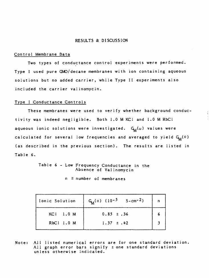
RESULTS & DISCUSSION
Control Membrane Data
Two types of conductance control experiments were performed.
Type I used pure G'v\O/decane membranes with ion containing aqueous
solutions but no added carrier, while Type II experiments also
included the carrier valinomycin.
Type I Conductance Controls
These membranes were used to verify whether background conduc-
tivity was indeed negligible. Both 1.0 M KCl and 1.0 M RbCl
aqueous ionic solutions were investigated. (\,,(w) values were
calculated for several low frequencies and averaged to yield (\,,(o)
(as described in the previous section). The results are listed in
Table 6.
Table 6 - Low Frequency Conductance in the Absence of Valinomycin
n = number of membranes
Ionic Solution ~(o) (10-5 S-cm-2)
KCl 1. 0 M 0. 85 ± .36
RbCl 1. 0 M 1. 37 ± • 42
n
6
3
Note: All listed numerical errors are for one standard deviation. All graph error bars signify ±one standard deviations unless otherwise indicated.

73
As these conductances are two to three orders of magnitude less
than the corresponding carrier-mediated transport, this background
conductance was ignored in all subsequent calculations.
Type II Conductance Controls
These membranes were used for periodic checks of valinomycin
quality and for comparison with conductance values reported in the
literature. ~(o) values for both de and low-frequency ac membranes
for various concentrations of metal ions were obtained (see Table 7).
The de measurements were repeated periodically to insure that
variations in the measured conductance and calculated rate
constants were not due to valinomycin degradation during storage.
Although not exact, Table 7 does illustrate reasonable agreement of
the conductance values and no valinomycin degradation was observed.
Capacitance Controls
Type I conductance control membranes were also used for com
parisons of ~ values. Control ac membrane~ values were obtained
and are listed in Table 8.
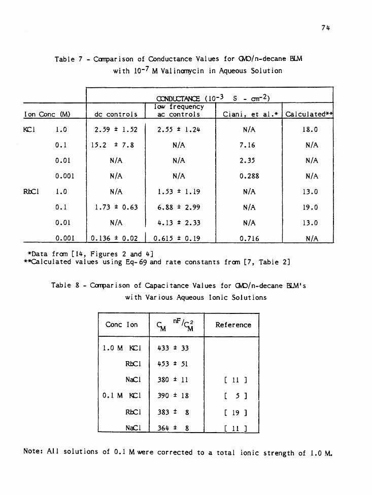
Table 7 - Canparison of Conductance Values for 0..0/n-decane Bl.M
with io-7 M Valinanycin in Aqueous Solution
<DIDLCTAl\CE ( 1 o-3 s - an-2) low frequency
74
I on Cone (M) de controls ac controls Ciani. et al.* CalculatedH
KC! 1.0 2.59 ± 1.52 2.55 ± 1.24 N/A 18.0
0 .1 15.2 ± 7.8 N/A 7 .16 N/A
0.01 N/A N/A 2.35 N/A
0.001 N/A N/A 0.288 N/A
Rb:! 1.0 N/A 1.53 ± 1.19 NIA 13.0
0 .1 1.73 ± 0.63 6.88 ± 2.99 N/A 19.0
0.01 N/A 4.13 ± 2.33 N/A 13.0
0.001 0.136 ± 0.02 I 0.615 ± 0.19 0.716 N/A
*Data fran [14, Figures 2 and 4] **Calculated values using Eq-69 and rate constants fran [7, Table 2]
Table 8 - Canparison of Capacitance Values for GVO/n-decane EL\lt's
with Various Aqueous Ionic Solutions
Cone Ion ~ nF/~ Reference
1.0 M I<Cl 433 ± 33
llli:l 453 ± 51
NaCl 380 ± 11 [ 11 J
0.1 M I<Cl 390 ± 18 [ 5 J
llli:l 383 ± 8 [ 19 J
NaCl 364 ± 8 [ 11 J
Note: All solutions of 0.1 Mwere corrected to a total ionic strength of 1.0 M.

75
A question which inevitably arises is whether ~varies with
different ions or ionic concentrations. Benz and Janko [6] have
determined t~at there is no significant difference in the~ for
similar (same lipid/solvent) membranes, using either 0.01, 0.1 or
1.0 M NaCl, hence concentration variations of~ are negligible.
Table 8 indicates that Svi varies little, if at all, with the ion
used.
Although our values appear to be higher than those reported
in the literature, the difference can be accounted for by the fact
that our membrane areas were not corrected for bulging due to
hydrostatic pressure differences across the membrane. This pressure
gradient is created when the brush is placed in one side of the
aqueous container during membrane formation. The membrane is
easily distensible and will bulge into the solution with the lower
liquid level. Subsequent investigations by Bill Brown of our group,
using a modified ac apparatus, have noted a less than 6% decrease
in~ when the membrane is flattened by adding extra fluid to the
aqueous solution on the bulging side of the membrane and monitoring
~until a minimum value is obtained. A similar degree of bulging
in this experiment could account for a majority of the difference
in the~ values, while the remainder may be attributable to area
measurement errors. The area measurement itself contains intrinsic
observational errors which are greater than normal in comparison
with usual instrumentation errors. The error is larger since the
entire torus is not usually visible, which leads to errors in
diameter determination. In an effort to minimize this error,

76
the membrane diameter was measured several times and an average
value used for area calculations. The bulging was assumed to be
constant throughout the experiments (similar membrane formation
technique, same volume of aqueous solution, etc.) and a bulging
correction factor of 433/390 = 1.11 was applied to all membrane
areas employed in data reduction for comparison with literature
values. It should be noted that the only final parameter deter-
minations affected by the values of membrane area are ~S and
NMS (see Equations 28, 77, 82) although some of the variation of
conductance controls listed in Table 7 may also be explained by
membrane area errors.
Kinetic Parameters
Table 9 lists the ac relaxation times and amplitudes as calcu
lated by the curve fitting procedure discussed in the Data Analysis
section. The error ranges reflect membrane population variation
rather than systematic errors. Data analysis was performed only on
the second or subsequent runs on any given membrane. The first run
was disregarded to better insure that the membrane was stable and
any membrane which did not survive more than one automated run was
discarded from the data pool. Also listed for comparison are
corresponding Ci..•s and Z-•s derived from relaxation experimental data
(charge-pulse rate constants given by Benz and Lauger [7] were used
in Equations 71-75).
Table 10 gives the rate constants and the partition coef
ficient which corresponds to the kinetic parameters in Table 9

77
(Equations 78-81 are used to generate the rate constants from the
relaxation times and amplitudes). The error range for the charge
pulse rate constants [7, Table 2] have also been included.

Table 9 - A.C. Relaxation Times and i6iq>litudes
T'l (µ,sec) T2 (µ,sec) a1 a2
1.0 M ~l
fran A.C. 1.50 ± 0.27 7 .55 ± 1. 33 0.768 ± 0.072 0.172 ± 0.005 experiment
derived fran 1.18 4. 89 0.370 0.512 Relaxation experiment*
1.0 M Rn:l
A.C. 0.63 ± 0.10 4.86 ± 0.27 0.882 ± 0.049 0.111 ± 0.045
Relaxation l.05 3.75 0.424 0.510
0.1 M Rn:l
A.C. 0.40 ± 0.15 3.72 ± 0.74 0.884 ± 0.055 0.084 ± 0.040
Relaxation 0.86 5.05 0.551 0.300
0.01 M Rn:l
A.C. o. 29 ± 0.19 2.59 ± 1. 36 0.925 ± 0.51 0.056 ± 0.041
Relaxation 1.09 5.23 0.608 0.117
*calculated fran ([25], Equations 5-9), using kinetic parameters given in [7].
n = mmber of membranes investigated.
78
n
4
9
4
7
8
8
8
7

79
Table 10 - Kinetic Parameters Corresponding to Table 9
kR kn ~ ks 'Ys
( 104 M-1 sec (104 sec-1 ) (104 sec-1 ) (104 sec- 1 ) (103)
l.OMI<Cl
A.C. 10.9 ± 2.4 10.4 ± 2.1 28.2 ± 7.5 2.6 ± 0.5 2.1 ± 0.8
Relaxation 29 ± 4 27 ± 6 21 ± 4 3.8 ± 0.8 7.5
1.0 M Rtcl
A.C. 21.2 ± 1.0 13.6 ± 2.7 73.8 ± 13.7 0.8 ± 0.1 3.7 ± 1.8
Relaxation 37 ± 12 24 ± 6 27 ± 3 3.5 ± 0.4 5.3
0.1 M Rl:Cl
A.C. 224 ± 85 24.6 ± 5.7 134 ± 60 4.3 ± 1.0 2.6 ± 1.2
Relaxation 190 ± 40* 38 ± 15 35 ± 13 4.5 ± 1.0'\- 8.1
0.01 MRtcl
A.C. 4550 ± 3910 19.4 ± 7.2 207 ± 84 6.8 ± 2.3 1.3 ± 1.1
Relaxation 630 ± 300 31 ± 3 29 ± 5 7.8 ± 0.5 8.6
*All pairs of ac and relaxation means differ significantly ( ?"' > • 0 5 ) ex c e p t f o r 0 • 1 M RbC l ( kR and k 5 ) as i n d i ca t e d •

80
Although the ac data error bars reflect scatter among the
membranes, there is also the possibility of systematic errors in
the determination of the solution resistance (Rs>· As outlined
under Data Analysis, the standard procedure actually produces
three values for Rs from which only one value was selected to be
used in the subsequent data reduction. The three values of Rs
usually varied from the mean by 1-3% (~0.5 - 1.50) for a particu-
lar membrane data run. However, for a given ionic concentration
the overall agreement of Rs between different membranes is quite
good. Table 11 lists the overall variation of the chosen
Rs values for all membranes in a particular aqueous solution.
Table 11 also shows (at least for 1.0 M RbCl or KCl) that Rs does
not clearly correlate with the concentration of valinomycin.
In order to determine the additional rate parameter error due
to this uncertainty in RS a membrane data run was reanalyzed. The
original Rs value was varied by the pessimistic uncertainty of
! 1.50 and used to produce new sets of conductance values from
which the rate constants are determined as before. Table 12 lists
the results, while Table 13 shows the additional uncertainties (~%)
in the a.c. experimental kinetic parameters and rate constants.
Although the parameters are all sensitive to variations in Rs the
differences are usually insufficient to fully reconcile these values
with those derived from the relaxation experiments.

Table 11 - Variation of Solution Resistance with Ionic Concentration
n' ~ total number of membrane data runs
R5(0)
KCl 1.0 M 85.4 ± 3.0
c lo-7 valin 82.6 ± 1. 6
RbCl 1. 0 M 84.9 ± 0.7
c lo-7 val in 89.4 ± 2.9
0. 1 M c 10-7 val in 115.6 ± 1. 2
0.01 M c io-7 val in 141 . 4 ± 9.6
81 .
n '
12
16
5
14
15
23
Table 12 - Variation in Rate Parameters due to Uncertainty in R5 Data from 0.1 M Rb+ C io-7 M valinomycin membrane
*From Tables 9 and 10
Kinetic Solution Resistance (RS) Relaxation
Parameter 116.5n 115 n 113.50 Values*
al .6364 .8625 .9225 .551
a2 .2718 .1029 .0577 .300
T 1 (µ,s) .4729 .3237 .2845 .8613
T 2 (µ,s} 3.533 3.531 3.581 5.047
k ~ -1 -1 R M-S' • 289 x 107 .231 x 1 o7 .214 x l 01 .190 x 107
kn (s-1) .593 x 106 .465 x 106 .240 x 106 .380 x 10 6
~s (s-1) • 711 x 106 .135 x 107 .163 x 107 .350 x 106
ks <s-1) .463 x 105 .414 x 1 o5 .404 x 105 .450 x 1 o5

Table 13 - Percent Variation in Rate Parameters
Parameter
a, l
a, 2
T1
T2
due to Uncertainty in RS
from data in Table 12)
/]. % Rate Constant
+5/-25 kR
+150/-50 kD
+50/-10 kMS
+O/ -1 ks
(determined
/]. %
+25/ -5
+25/-50
+20/-50
+10/ -2
82
I

83
Loss Tangent Results and Discussion
Due to the ambiguities in determining the membrane area,
discussed above, an alternative data analysis was also carried out
[36]. This involves comparing experimental curves of loss tangent
vs. frequency to curves obtained on the basis of parameters from
relaxation experiments. The loss tangent, LT, is defined by:
LT : ~ I w~ Eq-92
With such a ratio of capacitance and conductance, the area factor
in each value cancels and that source of error is removed.
Figures 17 through 20 give the loss tangents as calculated from
the normalized ac and relaxation data.
The 1.0 MK+ and Rb+ curves (Figures 17 and 18) from ac data
faithfully reproduce the general shape of the relaxation curves,
but there has been a general shift downward, indicating a relatively
constant difference in the loss tangent magnitude throughout the
entire frequency range.
The 0.1 and 0.01 M Rb+ curves (Figures 19 and 20) exhibit the
same curve shape duplication with a shift in magnitude at the
lower frequencies. However, at higher frequencies there is a
definite discrepancy. While the relaxation data curves continue
to tail off downward, the ac curves plateau and begin to rise by
300 KHz. It should be noted that the 200 KHz point of the ac data
lies consistently above its anticipated position in both the
1.0 MK+ and 1.0 M Rb+ curves. This peculiarity is believed to be
an artifact due to an electronic problem with the microprocessor
unit.

z <t 1-
cn en
>-l&J ~
g 0
.s " c cj <i. 0
c: 0 ·-... " • a Qi a:
I
0 0 -
84
...... N :i: ~ -0
"" a:: LI.
.5
~ 0 c = a > 2 ~
'o --~ 2
9

LO
SS
TA
N
101
10°
10-•
0 0
0 o
oo
0
1.0
10.0
0
KEY
o A.
C.
Da
ta
-R
elax
atio
n --
--3
Ca
pa
cito
r M
odel
I '<
~1
..
10
0.0
.. .. ' ' ' .. ' ' '
' ' ' ' '
' ' ..
10
00
.0 F
RE
Q (
KH
z)
Fig
. 18
L
oss
T
an
ge
nt
Cur
ves,
I.
0 M
R
bCI,
I 0-7
M
Vo
lino
myc
in
00
V
t

-;; 'O 0 2 ~
0 c: .. a 0 Ci .. -a .. 0 0 a a..
)( c > cj a (J ll.I -
<i CD ~ a: ft)
I I
0 I I I
z ~ en Cf)
0 0 _J 00
/ 1-<>--t. /
I I
I I , , , , ,
I I
I I
I I
I I
I I
I I
I
, , , , ,
, , , , ,
iO
0 ci 0 0
0 ci 0
0. 0
q
86
-N :c ~ -0 ll.I a:: .....
c: -(,) >. E 0 c: --0 > ~ ,... I 0
(.) ..a a:. 2
ci (I)
CD > ... ~ (J ... c: CD
"' c: ~ (I) (I)
0 _J
m
cit LL.

LO
SS
T
AN
101
10°
10-•
0
1.0
10.0
KEY
o A
.C.
Da
to
-R
ela
xati
on
----
3 C
ap
aci
tor
Mod
el
0 0
0 I
._.. " '
' ' '
' ' ' ',
, ' ....
10
0.0
... I J
' ' '
' .... ' .....
..... ' '
' .....
' '
IOO
O.O
Fig
. 2
0 Lo
ss
Tan
gent
C
urve
s,
0.01
M
R
b C
l,
10-7
M
Val
inom
ycin
F
RE
Q(K
Hz)
0
0
........

88
In an effort to understand the cause of the high frequency
discrepancy between the loss tangent curves for 0.1 and 0.01 M Rb+
the relaxation curves were recalculated. Figures 21 through 24
give the results after individually varying each rate parameter to
the extremes of its error range (as reported in [7]). Curves were
also obtained for each parameter being a factor of ten greater
than reported in [7]. Although these values are outside of the
reported error ranges, it does place each rate constant closer to . the ac values and would hopefully give an indication as to which
constants would be most likely to account for the LT curve
differences.
From the graphs in Figures 21 to 24, the following obser-
vations can be made: the low frequency range of the loss tangent
curve is sensitive to variations in k0 , k5 and to a lesser degree
kR while the high frequency range is predominantly affected by
changes in kR and kMs· Therefore, the discrepancy in the high
frequency portion of the loss tangent curve is probably due to
differences between kR and/or kMS between the two experiments.
Three Capacitor Model
The membrane model assumed by Laug~r and which forms the
basis for the analysis previously discussed in this thesis con-
siders the membrane as if it were a single dielectric slab.
However, a three slab-capacitor has been proposed as a more
realistic model. This consists of two identical external regions

LO
SS
TAN
KE
Y
10
1
10
°
10-1
', ',
A
kR ,
upp
er e
rro
r ra
nge
B
" ,
low
er e
rro
r ra
nge
c II
•
x 10
',
------
-'
---,
',
--
',,
', --
' '
-',
·,,
/ ' c
'
, '
/ ,,
/
',,
_,
',,
----"'-
------
'-.._
------,
----
-----
-,_ --
.......
.... ....
..........
.. ',
....
... '
........
',
........
' .....
... ',
' ...
. , ',
',
, ',
A
'
',
', ' ' B
1.0
10.0
1
00
.0
10
00
.0
Fig
. 21
L
oss
T
ange
nt
Per
turb
atio
ns
with
V
ari
atio
ns
of
kR
0. I
M
R b
CI I
I 0
-1 M
V
alin
omyc
in
FR
EQ
(K
HZ
) 0
0
\D

LOSS
TA
N
101
10
°
10-1
',,'',
,, ' '
1.0
', ' ' '
, ' ' ',
' ' ' '
' ' ' '
' ,, '
10.0
KEY
A
k 0
, up
per
erro
r ra
nge
B c ' ,, ' '
11
, lo
wer
err
or r
ange
II
t
X 1
0
' ... -::
:.:---
----....
........ .
.. .....
.......
... ......
' ' ' '
', ..
....
... ,
... ,,
'...
',
' ' ' ' '
' '
... ,
' ... ,
'
' ' ' '
',
',
...... ,
',
' ' ' '
' ',
' '...
'e
' ' ' ' c
', ' ~, ',
' ' A
10
0.0
1
00
0.0
FR
EQ
(K
HZ
) F
ig.
22
L
oss
T
ange
nt
Pe
rtu
rba
tion
s w
ith
Va
ria
tion
s o
f k
0 0.
I M
Rb
Cl,
10-
7 M
V
alin
omyc
in
\0
0

LOSS
TA
N
101
10°
10-1
·
1.0
10.0
KEY
A
kM
s' up
per
err
or
rang
e B
11
,
low
er e
rro
r ra
nge
c II
t
X IQ
..._.
- ... ......
.. ......
""'..
. "'C
.....
.... ~..
.....
..........
.... ,,,
, .... ,,
.........
.,,. ...
10-0
.0 .. ,_
.:: ... -
:-... ,,
........
. ',
, .....
.... ',
',
',
',A
'',
,,, ', B
10
00
.0
FR
EQ
(KH
Z)
Ffg
. 23
L
oa
a
Tan
gent
P
ertu
rbat
ion&
wit
h
Var
iatio
n& o
f k M
S
0.1
M
Rb
Cl,
10
M
V
alln
omyc
in
\0 -

LOSS
T
AN
101
T
10
° -r
10-1
Fig.
2
4
KEY
,A
,, c
A
k 8
, up
per
erro
r ra
nge
' '
' '
' '
' ' B
', '
, '
B
II
• lo
wer
err
or r
ange
'
' '
',
' '
' '
' •
' '
' c
• x
10
' ' ',
' '
' '
' '
' '
' '
' '
' '
' '
' '
' '
' '
' '
' '
~
' ' '
~ ' '
' ~
' '
~ '
' ' '
' '
,,
' ' .....
.....
' .....
.....
' ' ' '
....
1.0
10
.0
10
0.0
Lo
ss
Tan
gent
P
ertu
rbat
ion&
with
Var
iatio
ns o
f k
-7
s 0.
I M
Rb
Cl,
10
M
V
alin
omyc
in
10
00
.0
FRE
Q
(KH
Z)
\D
N

93
(consisting of the polar heads with part of the adjacent hydro
carbon and aqueous regions characterized by capacitance~)
sandwiched about a single internal capacitance (capacitance CI'
corresponding to the hydrophobic, non-polar lipid tail region as
envisioned in Figure 25.
In this model the applied ac voltage would be capacitively
divided across the three regions so that both the surface reac-
t ions and charge translocations are voltage driven. In a typical
case, where approximately 8% of the applied ac voltage is assumed
to drive the interfacial reactions, the data analysis yields
relaxation parameters which differ from those obtained when the
voltage is assumed to act only on the translocation process by the
following percentages:
-2%
+0.5%
-6%
+40%
The rate constants from [7] and values of CE and CI are similar
to estimates made by Coster, et al. [15] and Pickar and Amos [49]
in such a model (see Appendix B for details) to produce loss tangent
curves. Figures 17-20 illustrate the relative insensitivity of
the LT curves to the choice of a three capacitor model.
This model also predicts a slight rise in the capacitance
values for applied frequencies less than 1 KHz, an effect which
has been observed in our data and is not predicted by relaxation
theory.

• I I I
r-'\AAAAI : '-../\/IV V Vy, :
r'\ l A A ~ '-A.l!VVV~
~ ~""~~ I IVVVV\...../
I ' I I I I I
Fig. 25 Three Capacitor Model
C = External Capacitance E
C 1 = Internal Capacitance
94

95
These preliminary investigations would seem to indicate that
the parameters derived from the three capacitor model might not
vary as markedly from the relaxation values as our values do.
However, further experiments are necessary to confirm these
findings.

CONCLUSIONS
In this experiment we have measured the frequency dependence
of the membrane admittance for a series of glycerylmonoolein I l-:
n-decane bilayers in various aqueous ionic solutions ~ich also
contained the ion carrier valinomycin. The admittance data was
then normalized and curve-fitted to produce relaxation times and
amplitudes which in turn allowed the calculation of the kinetic
rate parameters as deduced from a single slab dielectric membrane
model. These ac experimental rate constants were then compared
with those obtained from charge-pulse relaxation methods.
It is clear that in most cases these two sets of values do
not agree. However, with the exception of the 0.01 M Rb+ case,
the discrepancies are not extreme. The largest range of variations
appears in the relaxation amplitudes and times (Table 9) but seem-
ingly these differences partially compensate to allow more even
agreement of the kinetic parameters (Table 10). Although the
absolute values vary, it should be noted that a similar trend is
present in the values for both types of experiments, e.g. kR
increases with decreasing ionic concentration.
A careful consideration of both random and systematic errors
does bring the two sets of values closer together but cannot fully
reconcile the differences. The discrepancies may also reflect the
need for changes in the basic model, which was a major reason for
performing the ac experiments in parallel with relaxation studies.

97
In order to assess this possibility one must decide if the experi
mental ac data fits the original model. One way to check this
possibility is by using the experimental parameters, which are
obtained from a fit to conductance data, to reconstruct the capa
citance. Table 4 illustrates the good agreement between the
reconstructed and experimental· capacitance values.
The model used to interpret the data contains a number of
simplifications. For instance the association and dissociation
reactions are assumed to be single step rather than multistep.
Also, the translocation processes are not strictly monomolecular
transitions over a single narrow barrier but rather are diffusive
movements across relatively broad barriers. The membrane was con
sidered to be of uniform thickness throughout the course of the
experiment while in reality thermal fluctuations probably cause
inhomogenous variations of the thickness with time. This, in
turn, would lead to a spectrum of k5 , kMS and time constants rather
than discrete values. Another simplification previously discussed
is the single dielectric slab employed in this model versus the
possible three capacitor model. It is possible that these simpli-
f ications to the model have a different influence on the calculated
rate constants in the relaxation and ac techniques. However, this
does not explain the larger discrepancies at 0.01 M RB+ when
compared to the variations at the other ionic concentrations.

98
Definitive answers to these questions cannot be obtained from
this research. A possible solution would be to perform both
relaxation and ac studies on ,each individual membrane. Another
improvement would be to extend the frequency range of the exper
iment. The waveforms at 100, 200 and 300 KHz are not as pure as
those at lower frequencies. In addition future analysis will
include careful correction of the data for control membrane
conductance, which decreases the discrepancy between the ac and
relaxation results. This correction has been applied to some of
the data for 0.1 M Rb+ since completion of this work, and the
resultant agreement is highly encouraging [38]. Refinements to
the experimental method (improved lighting, membrane area deter
mination, membrane flattening, etc.) are also desirable. Indeed,
some of these improvements have already been incorporated into the
experimental procedures of other researchers in the membrane
biophysics group.

REFERENCES
1. Ab r ah ams s on , S . and Pas ch e r , I rm i n [Ed s • ] , 1 9 7 6 : S t r u c t u r e of Biological Membranes. Plenum Press, New York.
2. Ait'yan, S.K., Markin, V.S. and Chizmadzhev, Y.S., 1973: Theory of the passage of alternating current across artif icial membranes in the carrier scheme. Biof izika 18:75.
3. Bamberg, E., Lauger, P. and Walz, D., 1969: cal effects in lipid bilayer membranes; I. Biophys. J. 9:1150.
Nonlinear electrilon injection.
4. Benz, R., 1972: Kinetik des carrier transportes durch bimolekulare phospholipid membramen. Thesis, University of Konstanz, Konstanz, West Germany
5. Benz, R., Frohlich, o., Lauger, P. and Montal, M., 1975: Electrical capacity of lipid bilayers made from monolayers. Biochim. Biophys. Acta. 394:323.
6. Benz, R., Janko, K., 1976: Voltage-induced capacitance relaxation of lipid bilayer membranes, effects of membrane composition. Biochim. Biophys. Acta. 455:721-738.
7. Benz, R. and Lauger, P., 1976: Kinetic analysis of carriermediated ion transport by the charge-pulse technique. J . Memb r an e Bi o l • 2 7 : 1 7 1 -1 91 •
8. Benz, R. and Stark, G., 1975: Kinetics of macrotetrolideinduced ion transport across lipid bilayer membranes. Biochim. Biophys. Acta. 382:27-40
9. Benz, R., Stark, G., Janko, K. and Lauger, P., 1973: Valinomycin-mediated ion transport through neutral lipid membranes: Influence of hydrocarbon chain length and t emp e r at u r e • J • Memb r an e B i o l • 1 4 : 3 3 9 - 3 6 4 •
10. Bevington, P.R., 1969: Data Reduction and Error Analysis for the Physical Sciences. McGraw-Hill, New York.
11. Brown, W.C. and Pickar, A.D., 1983: Capacitance of bilayers in the presence of lipophilic ions. Biophys. J. 41:354a.
12. Callen, H.B .• and Green, R.F., 1952: On a theorem of irreversible thermodynamics. Phys. Rev. 86:702.
13. Chapman, D. [Ed.], 1968: Biological Membranes - Physical Fact and Function. Academic Press, London.
1 4 • Ci an i , S • , Gamba l e , F • , G l i oz z i , A. and Ro l and i , R. , 1 9 7 5 : Effects of unstirred layers on the steady-state and zerocurrent conductance of bilayer membranes mediated by neutral carriers of ions. J. Membrane Biol. 24:1-34.

100
15. Coster, H.G.L. and Smith, J.R., 1974: The molecular organisation of bimolecular lipid membranes. A study of low frequency Maxwell-Wagner impedance dispersion. Biochim. Biophys. Acta. 373:151-164.
16. Daniel, V.Y., 1967: Dielectric Relaxation, Chapters 1,5,7. Academic Press, London.
17. Eigen, M. and DeMayer, L., 1963: Relaxation Methods, in Technique of Organic Chemistry, Vol VIII, part II, pp. 895-1054. (A. Weissberger, ed.) Interscience, New York.
18. Eisenman, G. [Ed.], 1973: Membranes, (three volumes). M. Dekker, New York.
19. Fettiplace, R., Andrews, D.M. and Haydon, D.A., 1971: The thickness, composition and structure of some lipid bilayers and natural membranes. J. Membrane Biol. 5:277-296.
20. Frye, L. and Edidin, M., 1970: The rapid intermixing of cell surface antigens after formation of mouse-human heterokaryons. J. Cell Sci. 7:319.
21. Greenfield, S., Brostoff, S., Eylar, E.H. and Morell, P., 1973: Protein composition of myelin of the peripheral nervous system. J. Neurochem. 20:1207.
22. Hinkle, P.C. and McCarty, R.E., 1978: How cells make ATP. Scientific American 238:104.
23. Hladky, S.B., 1975: Steady-state ion transport by nonactin and trinactin. Biochim. Biophys. Acta. 375:350.
24. Knoll, W. and Stark, G., 1977: Temperature-jump experiments on thin lipid membranes in the presence of valinomycin. J. Membrane Biol. 37:13-28
25. Kolb, H.A. and Lauger, P., 1978: Spectral analysis of current noise generated by carrier-mediated ion transport. J. Membrane Biol. 41:167-187.
26. Laris, P.C., Bahr, D.P. and Chaffee, R.R.J., 1975: Membrane potentials in mitochondrial preparations. Biochim. Biophys. Acta. 376:415.
27. Lauger, P. and Stark, R., 1970: Kinetics of carrier-mediated ion transport across lipid bilayer membranes. Biochim. Biophys. Acta. 211:458.
28. Lauger, P., Benz, R., Stark, G., Bamberg, E., Jordan, P.C., Fahr, A. and Brock, W., 1981: Relaxation studies of ion transport systems in lipid bilayer membranes. Quarterly Rev. Biophys. 14, 4:513-598.

29. Lehninger, A.L., 1975: Biochemistry, Chapter 11. Worth Publishers, New York.
30. McConnell, H.M., 1976: Spin Labeling, Chapter 13. (L.J. Berliner, Ed.) Academic, New York.
101
31. McKusick, V.A., Neufeld, E.F. and Kelly, T.E., 1982: The mucopolysaccharide storage diseases. In The Metabolic Basis of Inherited pisease. (Stanbrury, J.B., Wyngaarden, J.B., Fredrickson, D.S., Goldstein, J.L. and Brown, M.S., Eds.) McGraw-Hill, New York.
32. McLaughlin, S.G.A., Szabo, G., Eisenman, G. and Ciani, S., 1970: Surface charge and the conductance of phospholipid membranes. Proceedings of the National Academy of Science, U.S.A. 67:1268.
33. Mitchell, P. and Moyle, J., 1969: Estimation of membrane potential and pH difference across the cristae membrane of rat liver mitochondria. European J. Biochem. 7:471-484.
34. Nyquist, H., 1928: Thermal agitation of electric charge in conductors. Phys. Rev. 32:110.
35. Nystrom, R.A., 1973: Properties of lipid films. In Membrane Physiology. Prentice-Hall.
36. Pickar, A.O. and Amos, W.O., 1976: Alternating current studies of charge carrier transport in lipid bilayers. Biochim. Biophys. Acta. 455:36-55
37. Pickar, A.O. and Hobbs, J., 1982: The influence of sterols on pentachlorophenol-induced charge transfer across lipid bilayers studied by alternating current methods. Biochim. Biophys. Acta. 693:221-236.
38. Pickar, A.O. and Cox, K.L., 1983: Alternating current studies of valinomycin-mediated ion transport across lipid bilayers. Biophys. J. 41:183a.
39. Pressman, B.C., 1968: Ionophorous antibiotics as models for biological transport. Fed. Proc. 27:1283.
40. Rothfield, L.I. [Ed.], 1971: Structure and Function of Biological Membranes. Academic, New York.
41. Rouser, G., Nelson, G.J., Fleischer, S. and Simon, G., 1968: In Biological Membranes, Chapter 2 (D. Chapman, Ed.) Academic, New York.
42. Shemyakin, M.M., Ovchimnikov, Yu. A., Ivanov, V.T., Antonov, V.K., Vinogradova, E.I., Shkrob, A.M., Malenkov, G.G., Evstratov, A.V., Laine, I.A., Melnik, E.I. and Ryabova, I.D., 1969: Cyclodepsipeptides as chemical tools for studying ionic transport through membranes. J. Membrane Biol. 1:402.

43. Singer, S.J. and Nicholson, G., 1972: of the structure of cell membranes.
102
The fluid mosaic model Science 175:720.
44. Smejtek, P. and Paulis-lllangasekare, M., 1979: Modification of ion transport in lipid bilayer membranes in the presence of 2,#-dichlorophenoxyacetic acid; I. Enhancement of cationic conductance and changes of the kinetics of nonactin-mediated transport of potassium. Biophys. J. 26:441-466.
45. Stark, G. and Benz, R., 1971: The transport of potassium through lipid bilayer membranes by the n~utral carriers vaJinomycin and monactin. J. Membrane Biol. 5:133-153.
46. Stark, G., Benz, R., Pohl, G. and Janko, K., 1972: Val inomycin as a probe for the study of structural changes of black lipid membranes. Biochim. Biophys. Acta. 266:603
47. Stark, G., Ketterer, B., Benz, R. and Lauger, P., 1971: The rate constants of valinomycin-mediated ion transport through thin lipid membranes. Biophys. J. 11:981-994.
48. Szabo, G., Eisenman, G. and Ciani, S., 1969: The effects of macrotetralide actin antibiotics on the electrical properties of phospho lipid bi 1 ayer membranes. J. Membrane Bio 1. 1: 346
49. Szabo, G., Eisenman, G., Laprade, R., Ciani, S. and Krasne, S., 1973: Experimentally observed effects of carriers on the electrical properties of bilayer membranes - Equilibrium Domain. In Membranes - A Series of Advances, Vol. II, pp. 179-328. (G. Eisenman, Ed.) M. Dekker, New York.
50. Szabo, G., Eisenman, G., McLaughlin, S.G.A. and Krasne, S., 1972: Ionic probes of membrane structures. In Membrane Structure and its Biological Applications, Vol. 195, pp. 273-290. (D. Green, Ed.) New York Academy of Sciences.
51. Weast, R.C., 1970: Handbook of Chemistry and Physics, E-67, F-152. CRC, Cleveland.

103
Appendix A - Computer Printout Samples
REDU1
DATE 07/18/80 IvIEM# OJ RUN# 06
BRIDGE READINGS
F(KHZ) C(NF) G(UMHOS)
1 0.131 OVERRAN GE 2 0.208 OVERRAN GE 3 0.311 OVERRAN GE 4 0.515 OVERRAN GE 5 0.715 9.267 63.500 6 1.006 9.400 67.300 7 2.011 9.360 69.200 8 3.166 9.340 73.000 9 5.071 9.300 82.000
10 7.124 9.250 96.000 11 10.728 9.140 129.900 12 15.975 8.960 197.000 13 21.080 8.770 280.000 14 30.552 8.420 470.000 15 40.782 8.040 720.000 16 51. 071 7.660 1010.000 17 70.379 6.940 1610.000 18 101.297 5.830 2630.000 19 204.193 3.079 5390.000 20 295.308 1.869 6530.000 21 204.179 1.853 4603.000 22 295.234 1.038 5135.000 23 495.612 0.407 5710.000 24 693.528 0.214 5850.000 25 883.793 0.135 5880.000
CELL RESISTANCE COM?UTATIONS(OHMS)
FR.PTS. 25,24,23: 168.8 168.1 AV.168.4 AV.-51•1~117.3 FR.PTS. 24,23,22: 167.0 166.5 AV.166.8 AV. -51.1•115. 7 FR.PTS. 23,22,21: 165.6 166.5 AV.166.1 AV .-51.1=115.0
MEMBRANE PARAMETERS
CELL RESISTANCE=115.7

104
REDU1 - Continued
FREQ COND CAP LT D-LT RS KHZ MIC-SIEM NF OHMS
0.71 63.77 9.390 1. 5116 0.0008 ****** 1.01 67.41 9.533 1.1187 0.0006 8245.5 2.01 68.11 9.496 0.5676 0.0004 3578.1 3 .17 69.54 9.481 0.3687 0.0004 1721. 0 5.07 72.38 9.453 0.2403 0.0004 754.2 7.12 76.68 9.423 0.1818 0.0005 417.3
10.73 86.30 9.358 0.1368 0.0007 212.9 15.98 102.74 9.263 0.1105 0.0010 117.4 21.08 120.84 9.176 0.0994 0.0013 81.0 30.55 154.11 9.048 0.0887 0.0018 50.7 40.78 190.27 8.948 0.0830 0.0023 35.9 51.07 227.18 8.885 0.0797 0.0029 27.8 70.38 285.40 8.793 0.0734 0.0039 18.8
101.30 366.07 8.714 0.0660 0.0056 11.8 204.19 687.61 8.791 0.0609 0.0113 5.4 295.31 1034.0J 8.495 0.0656 0.0158 4.1
204.18 5145.36 6.276 0.6390 0.0113 56.4 295.23 7820.96 4.804 o.8775 0.0158 55.6 495.61 13049.53 2.907 1.4417 0.0279 51. 7 693.53 15729.77 1. 745 2.0683 0.0401 51.5 883.79 16883.61 1.118 2.7198 0.0521 52.2
REDU2
DATE 07/18/80 MEN!# 03 RUN# 06
CELL RESIST. COMPUT.(OHMS) HOBBS VERSION
FR.PTS. 25,24,23: 168.9 167.0 AV=167.9 AV.-51.1=116.8
FR.FTS. 24,23,22: 167.0 165.5 AV=166.2 AV.-51.1=115.1
FR.PTS. 23,22,21: 165.5 170.6 AV=168.0 AV.-51.1=116.9
CELL RESISTANCE=115.1
MEASURED MEMB AREA=0.181E-01 SQ CM
HF CAPAC(ASSUME GMO/DEC 1VIEMB)0.7835E-08
LOW FREQ MEMB PA~AMS(AV.): KHZ(MAX), SIEMENS, FARADS 2.01 0.6643E-04 0.94724E-08

REDU2 - Continued
DATA FOR CURVE FIT: 16 DATA PTS
FREQ
0.715 1.006 2.011 3.166 5.071 7.124
10.728 15.975 21. 080 30.552 40.782 51.071 70.179
101.297 204.193 295.308
TOTAL
NORM COND
1.000 1.015 1.025 1.047 1.090 1.156 1.303 1.554 1.832 2.347 2.911 3.493 4.432 5.787
11.487 17.796
INPUT PARAMETERS: ALPHA-1 =0.7000 ALPHA-2 =0.2000
TAU-1 =0.5000E-06 SEC TAU-2 =0.5000E-05 SEC
SUM OF SQUARES = 185.0
OUTPUT PARAMETERS: ALPHA-1 =0.9339 ALPHA-2 =0.5016E-01
TAU-1 =0.2971E-06 SEC TAU-2 =0.4045E-05 5EC
SUM OF SQUARES = 0.1872E-01
NORM CAP
0.949 1.000 1.000 1.000 0.988 0.969 0.929 0.872 0.818 0.740 o.678 o.64o 0.583 0.534 0.579 0.396
105
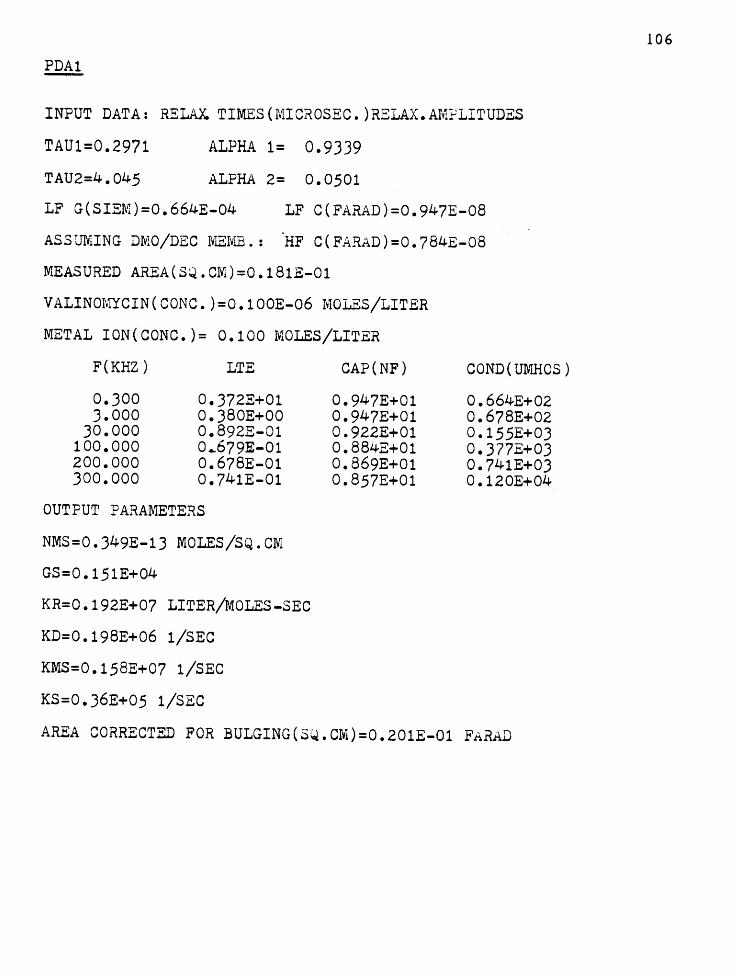
PDA1
INPUT DATA: RELAX. TIMES(MICROSEC.)RELAX.AMPLITUDES
TAUl=0.2971
TAU2=4.045
ALPHA 1= 0.9339
ALPHA 2= 0.0501
LF G(SIEM)=0.664E-04 LF C(FARAD)=0.947E-08
ASSUMING DMO/DEC MEMB.: .HF C(FARAD)=O. 784E-08
MEASURED AREA(SQ.CM)=0.181E-01
VALINOMYCIN(CONC.)=O.lOOE-06 MOLES/LITER
METAL ION(CONC.)= 0.100 MOLES/LITER
F(KHZ) LTE
0.300 0.372E+01 3.000 0.380E+OO
30.000 0.892E-Ol 100.000 0 .. 679E-01 200.000 0.678E-01 300.000 0.741E-01
OUTPUT PARAMETERS
NMS=0.349E-13 MOLES/SQ.CM
GS=0.151E+04
KR=0.192E+07 LITER/MOLES-SEC
KD=0.198E+06 1/SEC
KMS=0.158E+07 1/SEC
KS=O.J6E+05 1/SEC
CAP(NF)
0.947E+01 0.947E+01 0.922E+01 0.884E+Ol 0.869E+01 0.857E+01
COND(UMHOS)
0.664E+02 0.678E+02 0.155E+03 0.377E+03 0.741E+OJ 0.120E+04
AREA CORRECTED FOR BULGING(SQ.CM)=0.201E-01 FARAD
106

ADP1
RELAXATION TIN'lES ( MICROSEC.): GREQUENCY LIMITS(KHZ)
TAU1= 0.861 TAU2= 5.047 FRE1= 1161.871
F(KHZ) LTE
0.100 0.468E+02 0.200 0.234E+02 0.300 0.156E+02 0.500 0.936E+Ol 0.700 0.669E+Ol 1.000 0.469E+Ol 2.000 0.236E+01 3.000 0.159E+Ol 5.000 0.992E+OO 7.000 0.746E+OO
10.000 0.575E+OO 20.000 0.416E+OO 30.000 0.375E+OO 50.000 0.324E+OO 70.000 0.284E+OO
100.000 0.244E+OO 200.000 0~177E+OO 300.000 0 .140E+OO 500.000 0.949E•Ol 700.000 0.707E-01
1000.000 0.507E-01
KINETIC PARAMETERS:
GS=0.810E+04
KR=0.190E+07 LITER/MOLES-SEC
KD=0.380E+06 1/SEC
KMS=0.350E+06 1/SEC
KS=0.450E+05 1/SEC
THICKNESS=47.60 ANGSTROMS
CAP(NF)
0.64E+03 0.64E+03 0.64E+03 0.64E+03 0.64E+03 0.64E+03 0.64E+03 0.64E+03 0.64E+03 0.63E+03 0.63E+03 0.59E+03 0.55E+03 0.50E+03 0.48E+03 0.45E+03 0.42E+03 0.41E+03 0.40E+03 0.39E+03 0.39E+03
AREA=0.181E-01 CM-SQUARES
VALINOMYCIN(CONC.)=O.lOOE-06 MOLES/LITER
RBCL(CONC.)=0.100 MOLES/LITER
CI=7.06 NF
CON(UMHOS)
0.19E+05 0.19E+05 0.19E+05 0.19E+05 0.19E+05 0.19E+05 0.19:C+05 0.19E+05 0.20E+05 0.21E+05 0.23E+05 0.31E+05 0.39E+05 0.51E+05 0.59E+05 0.70E+05 0.94E+05 0.11E+06 0.12E+06 0.12E+06 0 .12E+06
107
FRE2= 198.129

APPENDIX 8
THREE CAPACITOR MODEL
Alternating current properties of the three-capacitor
model (Figure 25) can be calculated using a formalism similar
in some respects to that used by Ait'yan et al. [2] in their
general analysis of monomeric carrier schemes. This approach
to numerical modelling of a.c. electrical behavior has also
been applied to dimeric carrier transport systems by Pickar
and Hobbs [37].
The voltage ¢ impressed across the membrane is assumed
to divide across three membrane regions according to
Eq.-81
where ¢ 1 is the component of the voltage across the surface
layer bounded by the bulk aqueous solution and the adsorption
reaction plane on the left-hand side of the membrane (specific
capacitance CE), ¢2 is the component across the region interior
to the two adsorption-reaction planes (capacitance CI), and
¢3 is the component across the right-hand surface region
(capacitance CE).
1 ¢1 = C'
¢2 = 1 C'
¢3 = 1 C'
These component voltages are given by c c
{ c 1 ¢ - F ( 1+-c1 ) 6NM' s - F-1 6N 11 } E q- 8 2 E CE MS
r-,. ¢ + F6NMS F 6N II } -i. ""E MS Eq-83
c I I c
{CI¢ + FC 6NMS + F ( 1 +c1) 6N II }
E E MS Eq-84
where Fis the Faraday constant, the parameter C' = CE+2c 1 ,
and 6NMS and 6NMS are the surface concentrations in excess of

the equilibrium value of the loaded carrier in the left
and right-hand adsorption-reacti'on planes respectively.
109
The surface concentrations of free and loaded _carriers
vary in time according to the following differential
equations (Eqs-B5,B6,B7,B8) in which the voltage dependence
of the rate constants are given in explicit form:
dN' s = err
dN" s at = k (N'-N")-k C N11 exp(-Fct> 3 )+k N" exp(lli) s s s R M s 2RT D MS 2RT
k [ N I ( F ct> 2 ) N II· (' Fct> 2 ) J + MS MSexp 2HT - MSexp --2HT
In the above expressions the primes and douole-primes refer
to the left and right surfaces, respectively, and the surface
concentrations of permeable species are the total concen-
trations, i.e., N5' = N + ~N' etc. The interchange between s ·- s
the bulk aqueous solution and the membrane surface of the
neutral or loaded carrier (S or MS+) has been neglected.
In the absence of an applied voltage these equations yield
the equilibrium expression (previously Eq-21)
Eq-89

If a small voltage which is harmonic in form
<P = <Poexp(jwt) Eq-BlO
is applied, the perturbations from equilibrium of the
surface concentrations will, in the steady state, vary
sinusoidally in time with an angular frequency w. We
may then everywhere replace ~N~ by ~N~exp(jwt), ~NMS by
6NM5exp(jwt) etc., where the amplitudes 6N~, 6NMS' etc.
are now reganded as time-independent complex quantities.
We restrict our consideration of the problem to the case
of small voltage amplitudes. We can then use the approx-
imations = l + F<P1
- 2RT
+ lli - 2RT
exp(±F<P 3 ) = 1 + ~ 2RT - 2RT
Eq-Bl l
Furthermore, in the limit of very small voltages, after
substituting Eqs-B2,B3,B4,B8, and Bll into Eqs-85.through
110
88 we can neglect higher order terms such as those involving
(6N~) 2 , (6N~)(6NM5 ), (6N~)<Po etc. Time-independent terms
are eliminated by virtue of the equilibrium expression
Eq-89.
The resulting set of four inhomogeneous linear equations
in 6N~, ~N~, 6NMS' and ~NMS can be solved to permit compu
tation of the membrane admittance
YM = GM + jwCM = I/<P E q-B 1 2
where the membrane current I is given by

1 1 1
I = F 2 NMSkMS(~T) + FkMS(~NM 5 -~NM 5 )exp(jwt)+jwC 1 ¢2 Eq-813
We have made no attempt to write out the final expressions
for membrane admittance in closed form; instead, we have
used the above results to obtain numerical values of mem-
brane conductance GM and capacitance CM as a function of
frequency assuming various model parameters.