Alternative Approaches to Measuring MRP:

Are All Men’s College Basketball Players Exploited?

Erin Lane, Juan Nagel, and Janet S. Netz

March 2012

Abstract: College men’s basketball players have alleged that the NCAA’s illegal cap on

athletic scholarships leads to lower scholarships than would prevail in a free market. Recently,

the NCAA increased the limit on athletic scholarships. We compare the marginal revenue

product (MRP) of men’s basketball players to athletic scholarship caps. We estimate MRPs

using players’ playing statistics; information on the distribution of pro salaries; and players’

future draft status. We find that players’ MRPs are greater than the athletic scholarship caps for

about 60% of men’s basketball players, not just the star players.

Keywords: marginal revenue product, basketball

Acknowledgements: We gratefully acknowledge comments from Claudio Agostini, Brandon Netz, Josh Palmer (former UM point guard), and two anonymous referees. We were fortunate to receive comments from Gerald Scully on an earlier incarnation of this work.

Affiliations: All authors are affiliated with ApplEcon, LLC. Dr. Netz testified on behalf of Plaintiffs in White et al. v. NCAA. Juan Nagel is also affiliated with the Facultad de Ciencias Económicas y Empresariales, Universidad de los Andes. ApplEcon LLC, 617 E. Huron Street, Ann Arbor, MI 48104. (734) 213-1930 (voice), (734) 213-1935 (fax). erlane@applecon.com, jnagel@applecon.com, and netz@applecon.com.

1

Alternative Approaches to Measuring MRP:

Are All Men’s College Basketball Players Exploited?

March 2012

I. Introduction

In 2006, college men’s basketball players sued the NCAA, alleging that the NCAA fixed

the amount of athletic financial aid. At the time, the NCAA limited the total amount of financial

aid received by a student-athlete to a full grant-in-aid (full GIA), which covers tuition and fees,

room and board, and required textbooks. Though the case settled without changing the limit on

athletic scholarships, the NCAA increased the scholarship limit in 2011 by $2,000 to cover

incidental expenses such as school supplies other than required textbooks and travel between the

school and the student’s home.

The case and recent rule change highlight the question, Do student-athletes contribute

more to the school than they receive through athletic scholarships? We examine this question for

Division I men’s basketball players by estimating student-athletes’ marginal revenue product

(MRPs) using updated versions of two well-established approaches and one new approach.

In the first approach, we estimate MRP based on the student-athlete’s playing statistics.1

This approach produces a zero MRP estimate for student-athletes with no game play and, hence,

no playing statistics. These student-athletes contribute to the team’s performance despite the

lack of game play by providing scrimmage players for the starters and providing replacement

players should the starters be injured. Our second approach uses the distribution of NBA salaries

in conjunction with the MRPs estimated using the first method to allow for the computation of

MRPs for all team members, even those without playing statistics. The distribution of NBA

1 This approach follows the methodology developed and applied to baseball by Scully, 1974.

2

salaries provides information about the distribution of pro MRPs. We use the shape of the

distribution of pro MRPs to inform our calculation of college MRPs. . The final approach we

implement uses information on student-athletes who are ultimately drafted by the NBA.2 This

method provides an MRP estimate for all subsequently drafted players.

Previous estimates of the MRP of student-athletes do not include school fixed effects.

We estimate the MRP equations both with and without school fixed effects, and the results

indicate that school fixed effects are jointly significant. MRPs estimated using school fixed

effects are lower than those estimated without them, so previous MRPs may have been over-

estimated.

There is broad similarity in the results across all three methods, but notable differences in

the estimated MRPs as well. The average MRP for all men’s basketball players is about $90,000

with the Scully method and rises to almost $120,000 when information on the distribution of pro

MRPs is included, but the distribution of MRPs estimated by both approaches is similar. The

average MRP for star players – those who were ultimately drafted by the NBA – ranges from

$150,000 to $275,000 at schools with relatively low-revenue basketball programs and from about

$1 million to $1.4 million at schools with high-revenue basketball programs. The methods using

playing statistics show a significant range across MRPs for star players, while the Brown method

gives a single MRP estimate for all players at low-revenue schools and another for all players at

high-revenue schools.

We compare student-athletes’ MRPs to the previous and current limits on athletic

scholarships, as well as the cost of attendance (COA), which has been proposed as a limit on

2 This approach follows the methodology developed by Brown, 1993.

3

athletic scholarships.3 We believe that we are the first to tackle the question of whether the

revenue generated by all men’s basketball players – not just the star players – is greater than the

value of the scholarships that they receive. We find that about 60% of men’s basketball players

generated more revenue for their team than they received in the form of an athletic scholarship.

With two exceptions, the MRP of every player who was ultimately drafted by the NBA was

above the former and current scholarship limit.4

We proceed as follows. We first discuss the marginal benefits and costs of matriculating

a student-athlete in Section II, as these are the determinants, in part, of the athletic scholarships

offered by schools. We then discuss the estimation of MRPs using student-athletes’ playing

statistics in Section III; incorporating the distribution of pro salaries in Section IV; and using a

student-athlete’s future draft status in Section V. We compare the MRP estimates from the

different methods in Section VI. In Section VII, we compare the MRP estimates to the previous,

current, and proposed caps on athletic scholarships.

II. The Benefits and Costs of Student-Athletes

In a typical labor market, a profit-maximizing firm hires until the marginal revenue

product (MRP) is equal to the marginal cost of the last worker hired. In terms of collegiate

athletes, the “firms” “hiring” the student-athletes are non-profits with an objective other than

profit-maximization. However, in maximizing the alternative objective, whatever it may be, the

same economic principle applies: an athletic department or coach will take on a student-athlete

3 Most financial aid programs are based on a school’s cost of attendance. The COA covers tuition, room and board, and books (these items make up the GIA) as well as incidental expenses. The COA includes the full estimate of the incidental expenses, while the new NCAA limit only allows scholarships to cover up to $2,000 in incidental expenses. It is estimated that the estimated incidental expenses are $2,500 to $3,000 at most schools. 4 The exceptions are Joe Alexander at West Virginia and Dante Cunningham at Villanova, both based on freshman year only.

4

as long as his or her marginal contribution to the athletic department, team, or school is greater

than the marginal cost of taking the player on.

However, the NCAA limits the amount of each athletic scholarship. If this restriction

binds, student-athletes’ marginal contribution will be greater than their marginal cost.

A. Student-Athletes Do More than Generate Revenue

The direct benefit that a men’s basketball player brings to a school is to contribute to the

winning ability of the team. Increasing the team’s winning ability in turn translates into

additional revenue for the school: men’s basketball is one of the “revenue sports”, in that it often

generates net revenues for schools. Student-athletes themselves, or via their contribution to the

winning ability of the team, may generate benefits to schools other than generating basketball

revenues; for example, student-athletes’ performance may increase a school’s ability to recruit

students and attract additional donations.

Given the difficulties in quantifying the non-pecuniary contributions of a student-athlete

to the school, we limit our estimate of the marginal value of a student-athlete to his generation of

team revenues. The contribution of individuals to their sport’s revenues (their MRP) provides a

lower bound on the marginal contribution that a student-athlete provides to a school.

B. The Cost of a Student-Athlete

The cost to a school of taking on another men’s basketball player includes the marginal

costs of educating, housing, training, and playing the student-athlete. The most direct cost to the

athletic department is the value of his athletic scholarship. The player’s athletic scholarship may

not be a true reflection of the university’s cost of educating and housing the player. A large

portion of any scholarship is not a cash payment to the student-athlete, but a transfer from one

university account to another to cover tuition, room and board, and, often, even books.

5

These “transfer prices” do not necessarily represent the actual marginal cost to the school

for taking on another student. The marginal cost of another student may be considerably less

than tuition,5 and the marginal cost of lodging for a student may also be less than the charge for

room. The marginal cost of a student-athlete also depends on whether the student-athlete is an

additional student or is replacing another student, and if replacing a student, whether that student

would pay full price or receive financial aid from the school.

We do not have data to consistently and reliably adjust the scholarship to reflect the true

marginal cost to the school of granting the financial aid to the student-athlete. In addition, it is

typically the athletic department that determines whether to add a student-athlete, and under the

accounting systems of most schools, the athletic scholarship is a reasonable proxy of the direct

cost to the athletics department of adding a student-athlete to the team.

Other costs of adding a student-athlete include the costs of the arena and training

facilities, coaching, transportation, uniforms, etc. Many of the facilities are shared by other

sports (e.g., weight rooms, arenas, support services, administration) and the facilities are often

financed through sources not specifically attributed to men’s basketball. In addition, these latter

costs sometimes are provided by sources other than the school via sponsorships and donations.

For all these reasons, we limit our estimate of the marginal cost of a student-athlete to his

athletic scholarship.

C. Measuring the Benefits and Costs of a Student-Athlete

Colleges and universities must report revenues by sport to the Department of Education,

which include “revenues from appearance guarantees and options, contributions from alumni and 5 Martin, 2004, states that “Increasing returns to scale and significant fixed costs in the intermediate term imply that marginal cost [of college education] is less than average cost.” The article goes on to provide statistics from 1,600 liberal arts colleges that report average tuition and fees at $8,966, and a calculation of average marginal cost at $3,347.

6

others, institutional royalties, signage and other sponsorships, sports camps, state or other

government support, student activity fees, ticket and luxury box sales, and any other revenues

attributable to intercollegiate athletics.”6 Allocation of these revenues across sports requires

subjective decisions of the contribution of each sport, and are likely to differ from the revenues

the sports generate through these items. To the extent that the data include revenues not

generated by the basketball team (e.g., sports camps), the estimated MRP may be overstated.

Likewise, to the extent that the data exclude revenues generated by the basketball team (e.g.,

sales of team jerseys), the estimated MRP may be understated. Nonetheless, the allocated

revenue data are assumed to provide a reasonable, though imperfect, measure of the revenues

generated by the team.

We measure the direct marginal cost to the athletic department of adding a student-athlete

to the team with the maximum athletic scholarship. While we do not have data on the specific

value of the athletic scholarship received by each student-athlete, most men’s basketball students

receive the maximum allowable amount.7 Thus, the scholarship limit for men’s basketball

players at each school is an upper bound on the scholarship received by each player.

D. Individual Effort in Team Sports

Estimating a student-athlete’s marginal revenue product (MRP) is complicated in the case

of team sports in which players’ skills interact. To measure MRP, ideally one measures the full

output of the player; in a team sport, a player’s performance not only directly impacts the team’s

6 U.S. Department of Education, 2006, Glossary of Terms, http://www.ope.ed.gov/athletics/glossarypopup.aspx. Although government support is included, in practice most schools receive no government support. See NCAA College Athletics Finance Database, http://www.usatoday.com/sports/college/ncaa-finances.htm?csp=obinsite. 7 We calculate the average number of full GIA athletic scholarships given to men’s basketball players at Division I-A schools (total scholarship expenditures divided by the number of scholarships given). Because the average number of full GIA scholarships and the number of student-athletes receiving scholarships are roughly the same, we conclude that most basketball players receive the maximum athletics scholarship allowed under the NCAA rules.

7

performance but also can help or hinder teammates’ performance. Nonetheless, economists have

measured the MRP of individual athletes who participate in team sports, including basketball, by

using player performance as a reasonable proxy for the contribution of the player to team

performance.8 MRP for college basketball has only, to the best of our knowledge, been

measured for players who have ultimately been drafted by the NBA.

Measuring player performance is easier for some student-athletes and some positions

than others. In particular, it is difficult to measure the value of scrimmage players. The

scrimmage players often get little playing time (at the extreme, they may get no playing time and

thus may have no performance statistics), though having a decent set of backup players to

scrimmage against improves team performance. Young scrimmage players will also help in the

preparation of the school’s future team. In spite of their value to their school, these student-

athletes will not have performance statistics in the year they do not play, and will therefore

appear to have zero MRP.

III. Measuring MRP Using Players’ Playing Statistics

The first approach we use is based on the work of Scully (1974). First, the team’s win-

loss percentage is regressed on measures of team performance. Second, the team’s total

revenues are regressed on the team’s win-loss percentage, in addition to other determinants of

revenues. Finally, an individual player’s MRP is calculated as the product of the player’s

contribution to team performance, the marginal effect of team performance on the win-loss

percentage, and the marginal effect of the win-loss percentage on team revenues. We discuss the

8 See, e.g., Brown, 1993 (football), 1994 (basketball), and 2004 (football and basketball); Chatterjee and Campbell, 1994 (basketball); Hadley et al., 2000 (football); Hofler and Payne, 1997 (basketball); Leonard and Prinzinger, 1984 (football); Scott, Long, and Somppi, 1985 (basketball); and Zak, Huang, and Siegfried, 1979 (basketball).

8

source of our data in Appendix A, and present descriptive statistics for the variables used in our

study are included in Appendix B.

A. Step 1: The Win-Loss Regression

The team’s win-loss percentage in a season is modeled as a function of team performance

and the contribution of the coach. In mathematical terms,

itiitititit TXCPpct loss-win ε+λ+δ+γ+β+α= ,

where i indexes the team and t indexes the season. The vector P represents the team’s

performance variables, the vector C represents the team’s head coach’s contribution towards

winning, the vector X represents other determinants of the win-loss record, and the vector T

represents team-specific fixed effects.

We use standard team performance statistics as explanatory variables for win-loss

percentage:9 the number of blocks, steals, rebounds, and three-point shots per game and the

percentage of goals and of free-throws made. The number of blocks, steals, and rebounds per

game are measures of the team’s defensive performance. In all cases, the expected coefficient is

positive: the more blocks, steals, or rebounds, the better the defense and the more likely the team

is to win. The other variables are measures of the team’s offensive performance. The percentage

of shots that are made (field goals or free throws) indicates the scoring skills of the players, so

the higher these statistics, the more likely the team is to win.

We incorporate three variables to measure the head coach’s contribution to team

performance: a dummy variable indicating that there was a head coach change from the previous

season (“new coach”); a dummy variable indicating that the head coach was ranked “coach of

9 Measures of team productivity typically include variables related to shooting, rebounds, assists, steals, blocks, turnovers, and fouls. See Berri, 1999; Chatterjee and Campbell, 1994; Hofler and Payne, 1997; Scott, Long, and Sompii, 1985; and Zak, Huang, and Siegfried, 1979. Our data do not include data on turnovers or fouls.

9

the year” in the current season;10 and a continuous variable bounded by zero and one indicating

the coaches’ Division I win-loss record, for coaches who are currently ranked by the NCAA as

one of the “winningest coaches.”11

Coaches of the year and “winningest” coaches are particularly good and therefore their

teams should have more success, resulting in a positive coefficient on these variables. We are

agnostic as to whether the estimated coefficient on a coach change should be positive or

negative. On the one hand, it may be positive because often coaches are changed when the team

was doing poorly; thus, the new coach may be able to immediately increase the win-loss

percentage. On the other hand, the appointment of a new coach may hurt team morale, and in

the short-term there may be a reduction in the team’s win-loss percentage.12

We also include as explanatory variables the average rank index of opponents13 and the

number of games for each team that were televised. We include the opponents’ rank index to

measure the strength of opposition – the tougher the opposition, the lower the win-loss

percentage, and thus a negative coefficient is expected. Televised games may induce more effort

on the part of players, as televised games increase their exposure and may increase their chances

of being drafted. This effect would also lead to a higher win-loss percentage.

10 A coach is a coach of the year if he was so designated by UPI, The AP, the U.S. Basketball Writers Association, the National Association of Basketball Coaches, Naismith, The Sporting News, CBS/Chevrolet, or Basketball Times. 11 A “winningest coach” is one who has at least five years as a Division I head coach and has a win-loss record (for four-year U.S. colleges only) above 60%. 12 We do not believe that endogeneity is an issue with the coach of the year and “winningest” coach variables. While the coach of the year is the coach of the team with the highest win-loss record for half the seasons in the sample, for four of the six seasons, more than one coach was coach of the year. Furthermore, many coaches have very similar win-loss records for a given year, and most of these coaches are not coach of the year. The determination of “winningest” coaches is the coach’s win-loss record for his entire career at four-year schools as long as he’s been head coach of a Division I team for at least five years. Thus, the current year’s win-loss record is a small determinant of “winningest” coaches. 13 The rank index for a team for each week is calculated as 26 minus the team’s rank. Thus, as the rank index of opponents increases, the better are the opponents faced by the team.

10

We run two versions of the win-loss equation, with and without team fixed effects. Most

of the literature that measures productivity of teams does not include team fixed effects.14 We

include team fixed effects to capture the myriad inputs into a winning team that are difficult to

measure, such as the quality of the training facilities and academic support services available to

student-athletes. The exclusion of these factors may bias the MRP estimates by attributing some

of the win-loss percentage to the team’s performance rather than, say, the school’s superior

facilities.

We estimate the model using ordinary least squares (OLS).15 We present the results with

and without team fixed effects in Table 1.16

14 The only exception of which we are aware is Berri, 1999 (basketball). 15 The limited range of the win-loss percentage presents a potential econometric problem, since the assumption of the normal distribution of the error term under OLS requires that the dependent variable not be bound by zero and one. We also estimated the equation using a monotonic transformation of the win-loss percentage that is not bound by zero or one. The monotonic transformation is lwl = ln ( winloss / ( 1 – winloss ) ), where “ln” is the natural logarithm and “winloss” is the winloss percentage for each school-year pair. The results were not substantially affected by this transformation. 16 In addition to the two specifications we present, we explored others which varied in the included variables. All of them under-performed relative to the two that we present. These alternative specifications are available from the authors upon request.

11

Table 1: Scully Approach, Win-Loss Percentage Regression Results

Dependent Variable: Team’s Annual Win-Loss Percentage

No Team Fixed Effects With Team Fixed Effects

Independent Variables Estimated Coefficients

Standard Errors

Estimated Coefficients

Standard Errors

Constant –177.21*** 9.53 –162.56*** 11.30

Percentage Goals Made 343.57*** 15.23 318.29*** 16.82

Percentage Free Throws Made 51.24*** 10.12 61.46*** 10.65

Three Point Goals per Game 1.43*** 0.29 0.98*** 0.33

Blocks per Game 0.47 0.35 1.09*** 0.42

Steals per Game 1.19*** 0.26 1.90*** 0.28

Rebounds per Game 0.70*** 0.13 0.38 0.15

New Coach –2.03* 1.14 –1.66* 1.02

Coach of the Year 16.30*** 3.47 12.72*** 3.16

“Winningest” Coach 7.74*** 1.38 3.52** 1.66

Opponents’ Average Rank Index

–0.26 0.29 1.12** 0.45

Televised Games 0.27*** 0.05 0.19** 0.05

Team fixed effects included†

Adjusted R2 .55 .69

Number of Observations 1,044 1,044 *** Significant at the 1% level, ** at the 5% level, and * at the 10% level. † Jointly significant at the 1% level.

In general, the variables are statistically significant and of the expected sign. In

particular, the coefficients for the team performance variables are positive and generally

significant, although the coefficients on blocks per game and on rebounds per game are

insignificant in the version that excludes and includes team fixed effects, respectively. A coach

change leads to a reduction in the win-loss percentage, but the presence of a “coach of the year”

or a “winningest” coach increases the team’s win-loss record. The number of televised games

12

may be indicative of team spirit, which may explain why it increases the team’s win-loss

performance. The opponents’ average rank index negatively impacts a team’s win-loss

performance in the version that excludes team fixed effects, as expected, but has no significant

impact when team fixed effects are included.

The results support the inclusion of the fixed effects: the fixed effects are jointly

significant and the adjusted R2 increases substantially, from 0.59 to 0.72. Thus, unless otherwise

indicated, we focus on the results from the version that includes team fixed effects.

B. Step 2: The Revenue Regression

The team’s revenue is modeled as a function of team performance and demand. In

mathematical terms,

,rev itiiitititit TYearConfDTWL εληδγβα ++++++=

where i indexes the team and t indexes the season. The vector TWL represents the team’s

performance variables, D includes variables to measure other determinants of revenue, Conf

represents the team’s conference, Year represents the season, and T represents team fixed effects.

The vector TWL includes two variables. We include the win-loss percentage as a stand-

alone variable and interacted with a dummy equal to one for teams with large revenues. The

coefficient of the win-loss percentage in the revenue equation indicates the dollar increase in

revenues given an increase in the team’s win-loss percentage. We hypothesize that an increase

in the win-loss percentage will not represent the same increase in revenues for a school that

generates, say, $0.5 million per year in revenues from men’s basketball, as for a school that

generates $12 million. Therefore, we create a dummy variable equal to one if a team generates

13

more than $10 million in a given year.17 This allows for the possibility that the effect of win-loss

percentage on revenues is different for large teams. We expect the sign of the coefficient on both

win-loss variables to be positive – the more games won, the more revenue the team earns, with

the impact being larger at schools with more revenue.

To measure other revenue sources, we include variables (in the vector D) measuring the

team’s home-arena capacity and the capacity of opponents’ arenas, a dummy equal to one if the

team was sponsored by Nike, the team’s rank index in the previous three seasons and the average

rank index of opponents during the season (see footnote 13), and the number of games televised

during the season.

We include arena capacity for the team and its opponents as determinants of ticket

revenues; the more seats available, the more revenues that can be earned, and thus positive

coefficients are expected. The Nike dummy is included because schools sponsored by Nike have

access to the top high school recruits through their sponsorship deals and All-American camps.18

Recruiting top high school players should increase demand by fans to see games, increasing

ticket and broadcast revenues.

We include the team’s previous rank index to capture fan demand – teams that have been

performing well (poorly) should encourage more (less) fan demand this year – and thus we

expect a positive coefficient. We include the rank index of the opponents to account for the

17 The results for alternative definitions of large schools (i.e., schools with basketball revenues greater than $8, $9, $11, or $12 million) give similar results. 18 “Nike marketing consists of some 50 or 60 college sponsorships (though perhaps only half of these involve significant cash beyond the free outfitting), scores of individual athletes under promotional contracts, free sneaker deals with over 150 high schools and AAU (American Amateur Union) teams, summer sports camps for promising athletes, and sponsorships with professional teams in various sports.” Zimbalist, 1999.

14

quality and/or entertainment value of the games. We expect that better opponents will lead to

more demand, and thus expect a positive coefficient.19

Finally, we include the number of televised games as another indicator of demand,

expecting a positive coefficient. More televised games generally lead to more broadcast

revenues.

We include conference dummies to account for the different revenue-sharing policies

specific to each conference.20 We include year dummies to allow for the impact of general

macroeconomic conditions, as well as to indicate any impact on demand from exogenous events

(such as the winter Olympics in 2002).

Finally, we estimate the revenue equation with and without team fixed effects. Team

fixed effects are appropriate if, for example, a school gets more institutional support (which may

be in the form of student fees) or higher contributions to the athletics department if it is a big

sport school. This degree of support might continue in years when the team is not doing so well

(in terms of its winloss record). For example, the University of Michigan has one of the largest

bases of alumni in the country and is a reasonably strong basketball school. UM could therefore

raise more revenue than other schools, whether the team is currently doing well or not. All other

variables are included when team fixed effects are included.

Table 2 presents the results for the OLS regressions.21

19 Of course, it may be that the relative quality of the teams is what drives demand; that is, there may be more demand to see a game between two top ranked teams or two unranked teams, where the outcome of the game is more uncertain, than to see a game between a top ranked team and an unranked team. We tried including the absolute value of the team’s average rank and its opponents’ average rank, but that variable was insignificant. 20 For example, some conferences split gate revenues evenly; some split a minimum, with revenues above the minimum accruing to the home team; and some guarantee a minimum to the visiting team. These revenue-sharing rules thus impact the revenues earned by the school. 21 The limited range of the win-loss percentage presents a potential econometric problem, since the assumption of the normal distribution of the error term requires that the dependent variable not be bound by zero and one. We also estimated the equation using a monotonic transformation of the win-loss percentage that is not bound by zero or one.

15

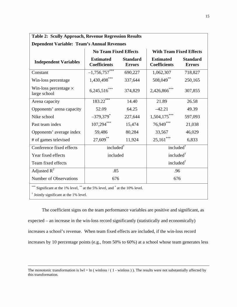
Table 2: Scully Approach, Revenue Regression Results

Dependent Variable: Team’s Annual Revenues

No Team Fixed Effects With Team Fixed Effects

Independent Variables Estimated Coefficients

Standard Errors

Estimated Coefficients

Standard Errors

Constant –1,756,757*** 690,227 1,062,307 718,827

Win-loss percentage 1,430,498*** 337,644 508,049** 250,165

Win-loss percentage × large school 6,245,516*** 374,829 2,426,866*** 307,855

Arena capacity 183.22*** 14.40 21.89 26.58

Opponents’ arena capacity 52.09 64.25 –42.21 49.39

Nike school –379,379* 227,644 1,504,175*** 597,093

Past team index 107,294*** 15,474 76,949*** 21,038

Opponents’ average index 59,486 80,284 33,567 46,029

# of games televised 27,609** 11,924 25,161*** 6,833

Conference fixed effects included† included†

Year fixed effects included included†

Team fixed effects included†

Adjusted R2 .85 .96

Number of Observations 676 676 *** Significant at the 1% level, ** at the 5% level, and * at the 10% level. † Jointly significant at the 1% level.

The coefficient signs on the team performance variables are positive and significant, as

expected – an increase in the win-loss record significantly (statistically and economically)

increases a school’s revenue. When team fixed effects are included, if the win-loss record

increases by 10 percentage points (e.g., from 50% to 60%) at a school whose team generates less

The monotonic transformation is lwl = ln ( winloss / ( 1 - winloss ) ). The results were not substantially affected by this transformation.

16

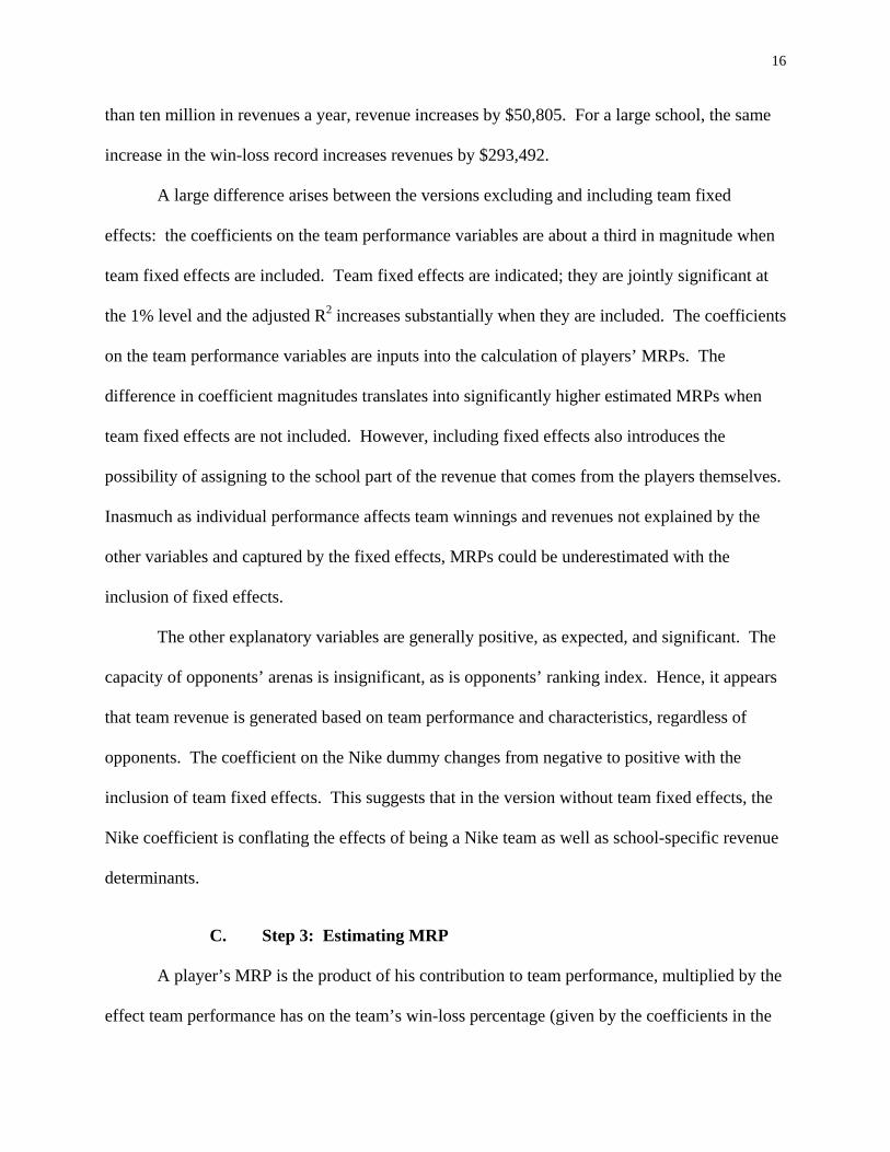
than ten million in revenues a year, revenue increases by $50,805. For a large school, the same

increase in the win-loss record increases revenues by $293,492.

A large difference arises between the versions excluding and including team fixed

effects: the coefficients on the team performance variables are about a third in magnitude when

team fixed effects are included. Team fixed effects are indicated; they are jointly significant at

the 1% level and the adjusted R2 increases substantially when they are included. The coefficients

on the team performance variables are inputs into the calculation of players’ MRPs. The

difference in coefficient magnitudes translates into significantly higher estimated MRPs when

team fixed effects are not included. However, including fixed effects also introduces the

possibility of assigning to the school part of the revenue that comes from the players themselves.

Inasmuch as individual performance affects team winnings and revenues not explained by the

other variables and captured by the fixed effects, MRPs could be underestimated with the

inclusion of fixed effects.

The other explanatory variables are generally positive, as expected, and significant. The

capacity of opponents’ arenas is insignificant, as is opponents’ ranking index. Hence, it appears

that team revenue is generated based on team performance and characteristics, regardless of

opponents. The coefficient on the Nike dummy changes from negative to positive with the

inclusion of team fixed effects. This suggests that in the version without team fixed effects, the

Nike coefficient is conflating the effects of being a Nike team as well as school-specific revenue

determinants.

C. Step 3: Estimating MRP

A player’s MRP is the product of his contribution to team performance, multiplied by the

effect team performance has on the team’s win-loss percentage (given by the coefficients in the

17

win-loss regression), multiplied by the effect that the increase in the team’s win-loss percentage

has on revenues (given by the coefficients in the revenue equation).

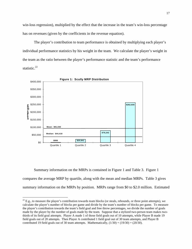
The player’s contribution to team performance is obtained by multiplying each player’s

individual performance statistics by his weight in the team. We calculate the player’s weight in

the team as the ratio between the player’s performance statistic and the team’s performance

statistic.22

$999 $20,941

$79,243

$262,935

$0

$50,000

$100,000

$150,000

$200,000

$250,000

$300,000

$350,000

$400,000

Quartile 1 Quartile 2 Quartile 3 Quartile 4

Average MRP

Figure 1: Scully MRP Distribution

Mean: $91,030

Median: $44,418

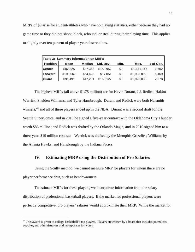
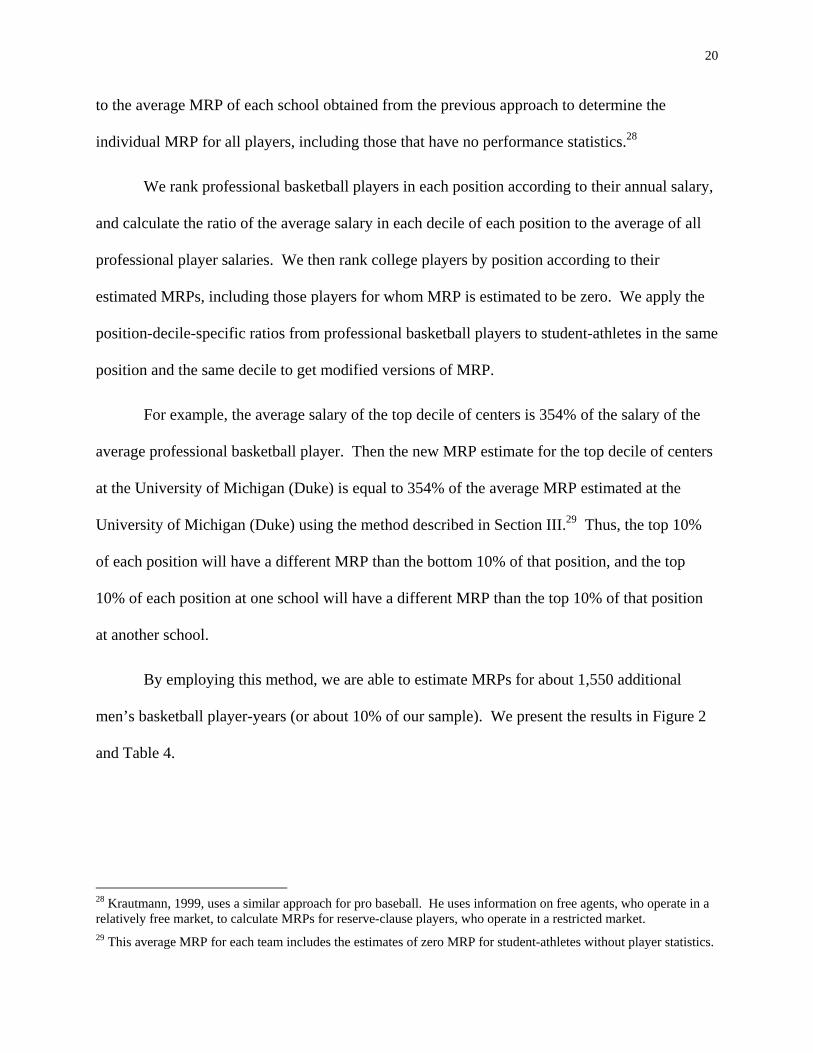
Summary information on the MRPs is contained in Figure 1 and Table 3. Figure 1

compares the average MRP by quartile, along with the mean and median MRPs. Table 3 gives

summary information on the MRPs by position. MRPs range from $0 to $2.0 million. Estimated

22 E.g., to measure the player’s contribution towards team blocks (or steals, rebounds, or three point attempts), we calculate the player’s number of blocks per game and divide by the team’s number of blocks per game. To measure the player’s contribution towards the team’s field goal and free throw percentages, we divide the number of goals made by the player by the number of goals made by the team. Suppose that a stylized two-person team makes two-thirds of its field goal attempts. Player A made 1 of those field goals out of 10 attempts, while Player B made 19 field goals out of 20 attempts. Then Player A contributed 1 field goal out of 30 team attempts, and Player B contributed 19 field goals out of 30 team attempts. Mathematically, (1/30) + (19/30) = (20/30).

18

MRPs of $0 arise for student-athletes who have no playing statistics, either because they had no

game time or they did not shoot, block, rebound, or steal during their playing time. This applies

to slightly over ten percent of player-year observations.

Position Mean Median Std. Dev. Min. Max. # of Obs.Center $87,325 $37,363 $158,952 $0 $1,671,147 1,702 Forward $100,567 $54,423 $17,051 $0 $1,998,899 5,469 Guard $91,491 $47,201 $158,127 $0 $1,923,038 7,278

Table 3: Summary Information on MRPs

The highest MRPs (all above $1.75 million) are for Kevin Durant, J.J. Redick, Hakim

Warrick, Shelden Williams, and Tyler Hansbrough. Durant and Redick were both Naismith

winners,23 and all of these players ended up in the NBA. Durant was a second draft for the

Seattle SuperSonics, and in 2010 he signed a five-year contract with the Oklahoma City Thunder

worth $86 million; and Redick was drafted by the Orlando Magic, and in 2010 signed him to a

three-year, $19 million contract. Warrick was drafted by the Memphis Grizzlies; Williams by

the Atlanta Hawks; and Hansbrough by the Indiana Pacers.

IV. Estimating MRP using the Distribution of Pro Salaries

Using the Scully method, we cannot measure MRP for players for whom there are no

player performance data, such as benchwarmers.

To estimate MRPs for these players, we incorporate information from the salary

distribution of professional basketball players. If the market for professional players were

perfectly competitive, pro players’ salaries would approximate their MRP. While the market for

23 This award is given to college basketball’s top players. Players are chosen by a board that includes journalists, coaches, and administrators and incorporates fan votes.

19

pro basketball players is significantly closer to a free market than is the market for college

players, it is not perfectly competitive. In particular, since the 1998-99 season, there has been a

cap on the total wage bill per team as well as a cap and floor on individual player salaries.24

The maximum player salary is a soft cap. For example, those players who already had

salaries above the maximum were grandfathered in, and only the first season’s salary is subject

to the maximum for multi-year contracts (although there is a limit on the size of raises from year

to year). In the first year under the new collective bargaining agreement (CBA), five pro players

signed new contracts at the maximum and eight had salaries beyond the maximum because they

were grandfathered in.25 Approximately 1% of pro players’ salaries were capped in the first year

of the CBA. For the 2002-03 season, approximately 17% of players were at the salary floor.26

While the salary caps and floor will mean that the salaries at the top and bottom end of the

distribution somewhat understate and overstate those pro players’ MRPs, we use the distribution

of pro salaries as a proxy for the distribution of pro MRPs.

We then assume that the shape of the distribution of MRPs of pro players mirrors the

shape of the distribution of MRPs of college players.27 The implication is that, for example, if a

benchwarmer center receives a salary that is 5% of the average NBA player, the benchwarmer’s

MRP is 5% of the average NBA player’s MRP. We apply the shape of the pro salary distribution

24 Staudohar, 1999. For players’ minimum and maximum salaries, see NBA Salary Cap FAQ, http://members.cox.net/lmcoon/salarycap.htm. 25 Hill and Groothuis, 2001, tables 1 and 2. 26 From Patricia Bender at http://www.Eskimo.com/~pbender/misc/salaries03.txt 2009. This includes all players signed, even those signed for 10-day periods and those released in the middle of the season. 27 We are not assuming the abilities of pro players are equivalent to the abilities of college players (hence the values of the MRPs for college and pro players are not assumed to be equal), nor are we assuming that a top-tier college player will be at the top end of the ability distribution when he goes to the pros.

20

to the average MRP of each school obtained from the previous approach to determine the

individual MRP for all players, including those that have no performance statistics.28

We rank professional basketball players in each position according to their annual salary,

and calculate the ratio of the average salary in each decile of each position to the average of all

professional player salaries. We then rank college players by position according to their

estimated MRPs, including those players for whom MRP is estimated to be zero. We apply the

position-decile-specific ratios from professional basketball players to student-athletes in the same

position and the same decile to get modified versions of MRP.

For example, the average salary of the top decile of centers is 354% of the salary of the

average professional basketball player. Then the new MRP estimate for the top decile of centers

at the University of Michigan (Duke) is equal to 354% of the average MRP estimated at the

University of Michigan (Duke) using the method described in Section III.29 Thus, the top 10%

of each position will have a different MRP than the bottom 10% of that position, and the top

10% of each position at one school will have a different MRP than the top 10% of that position

at another school.

By employing this method, we are able to estimate MRPs for about 1,550 additional

men’s basketball player-years (or about 10% of our sample). We present the results in Figure 2

and Table 4.

28 Krautmann, 1999, uses a similar approach for pro baseball. He uses information on free agents, who operate in a relatively free market, to calculate MRPs for reserve-clause players, who operate in a restricted market. 29 This average MRP for each team includes the estimates of zero MRP for student-athletes without player statistics.

21

$10,587$30,024

$71,406

$370,242

$0

$50,000

$100,000

$150,000

$200,000

$250,000

$300,000

$350,000

$400,000

Quartile 1 Quartile 2 Quartile 3 Quartile 4

Average MRP

Figure 2: Pro MRP Distribution

Mean: $117,764

Median: $39,750

Comparing the earlier results given in Figure 1 and Table 3, we see that the minimum

MRP is increased from $0 to about $3,500. The maximum MRP is also slightly higher, and the

median MRP is about 30% higher. We discuss the differences further in Section VI.A.

Position Mean Median Std. Dev. Min. Max. # of Obs.Center $128,355 $53,340 $277,349 $3,837 $1,777,842 1,702 Forward $124,909 $45,789 $281,768 $3,404 $2,038,780 5,469 Guard $117,503 $40,248 $271,884 $3,568 $1,882,623 7,278

Table 4: Summary Information on Pro MRPs

V. Estimating MRP using a Player’s Future Draft Status For men’s basketball players who are ultimately drafted into the NBA, we can also

estimate MRP using the method developed in Brown (1993). We estimate a model of team

revenue as a function of the number of star players (players who were ultimately drafted) in their

roster in each year and other determinants for revenue, as follows:

itiiititititit TYearConfDrgeDraftedxLaDraftedrev ε+λ+η+δ+γ+η+β+α= ,

22

where i indexes the team and t indexes the season. The variable Drafted represents the number

of players ultimately drafted by the NBA for all teams, while the interacted variable Drafted ×

Large represents the number of players ultimately drafted by the NBA for schools that had

annual basketball revenues greater than $10 million.30 The vector D includes other determinants

of revenue for the team; the vector Conf represents the team’s conference; the vector Year

represents the season; and the vector T represents team fixed effects.

The variables of interest are Drafted and Drafted × Large. The coefficient on the number

of drafted players (Drafted) indicates the dollar increase in revenues given an additional player

with enough talent to be drafted by the NBA at a low-revenue school, and the sum of the

coefficients on the two variables indicates the dollar increase at a large-revenue school. Thus,

the coefficient on Drafted is the MRP for star players at low-revenue schools and the sum of the

coefficients on Drafted and Drafted × Large is the MRP for star players at high-revenue schools.

To control for other revenue sources, we include the same variables as in the Scully

approach: the team’s home-arena capacity and the capacity of opponents’ arenas, a dummy

equal to one if the team was sponsored by Nike, the team’s rank index in the previous three

seasons and the average rank index of opponents during the season, and the number of games

televised during the season. These variables are all expected to have the same impact as before.

Again we estimate the equation with and without team fixed effects.

The number of players drafted is endogenous, correlated with unobserved factors that

also affect revenue.31,32 In particular, teams with higher revenues are likely to spend more on

30 The results are similar when a large basketball program is defined as revenue greater than $8, $9, $10, $11, or $12 million. 31 Endogeneity is confirmed with both Durbin and Wu-Hausman test statistics.

23

recruiting and attract better players who will later be drafted.33 To correct for the biases caused

by the endogeneity in the draft variable, we employ two-stage least squares (2SLS). The

excluded instruments are: the win-loss ratio; the numbers of points, goals, three-point goals,

blocks, rebounds, steals, and assists per game; the percentages of goals and free throws made;

whether the team was a contender or loser in the previous season; whether the head coach was

new, a coach of the year, or a “winningest” coach; and a measure of the market opportunities for

the school.34 The R2s for the first stage regressions are about 0.80, and a test of the over-

identifying restrictions confirms the validity of the instruments.

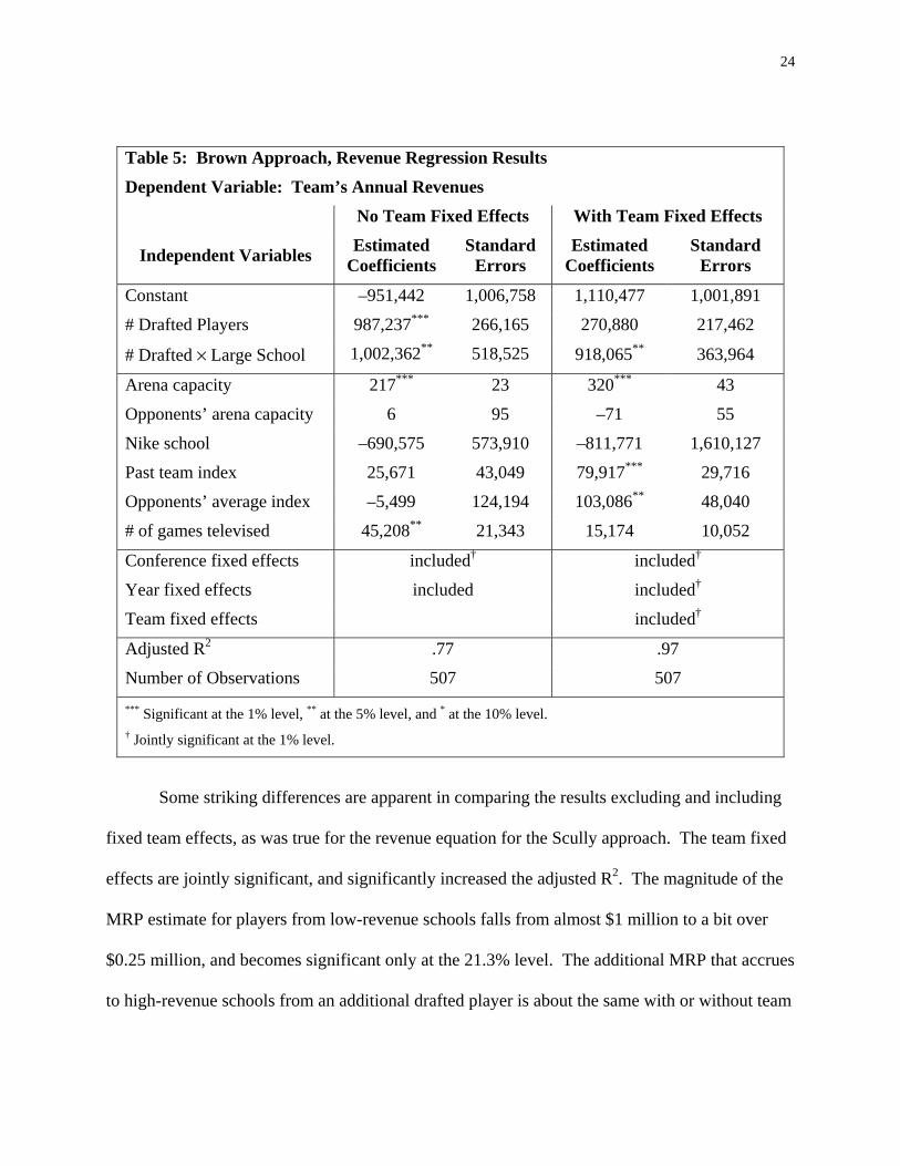
The results from the 2SLS Brown regression are presented in Table 5.

32 The winloss variables included in the revenue equation when estimating the MRP using the Scully approach could also be subject to a similar simultaneity issue. However, the Durbin and Wu-Hausman tests do not reject the null hypothesis of exogeneity. 33 NCAA rules limit recruiting activities under bylaw 13, but there is still variation in recruiting expenditures within the limits (and plenty of allegations of expenditures outside the limits). 34 The variable to measure market opportunities is based on Brown, 1993. We use a weighted average of population in 20-, 40-, and 60-mile diameters around the college, divided by the number of college and pro basketball teams within 60 miles.

24

Table 5: Brown Approach, Revenue Regression Results

Dependent Variable: Team’s Annual Revenues

No Team Fixed Effects With Team Fixed Effects

Independent Variables Estimated Coefficients

Standard Errors

Estimated Coefficients

Standard Errors

Constant –951,442 1,006,758 1,110,477 1,001,891

# Drafted Players 987,237*** 266,165 270,880 217,462

# Drafted × Large School 1,002,362** 518,525 918,065** 363,964

Arena capacity 217*** 23 320*** 43

Opponents’ arena capacity 6 95 –71 55

Nike school –690,575 573,910 –811,771 1,610,127

Past team index 25,671 43,049 79,917*** 29,716

Opponents’ average index –5,499 124,194 103,086** 48,040

# of games televised 45,208** 21,343 15,174 10,052

Conference fixed effects included† included†

Year fixed effects included included†

Team fixed effects included†

Adjusted R2 .77 .97

Number of Observations 507 507 *** Significant at the 1% level, ** at the 5% level, and * at the 10% level. † Jointly significant at the 1% level.

Some striking differences are apparent in comparing the results excluding and including

fixed team effects, as was true for the revenue equation for the Scully approach. The team fixed

effects are jointly significant, and significantly increased the adjusted R2. The magnitude of the

MRP estimate for players from low-revenue schools falls from almost $1 million to a bit over

$0.25 million, and becomes significant only at the 21.3% level. The additional MRP that accrues

to high-revenue schools from an additional drafted player is about the same with or without team

25

fixed effects, about $1 million.35 One interpretation is that without fixed effects a lot of the

school-specific variation was being attributed to the “performance” variables, and the number of

drafted players is now more precisely proxying for performance. Alternatively, because some of

the fixed effects are correlated with the other regressors, the estimated coefficients may conflate

the influence of the regressors and of the fixed effects.

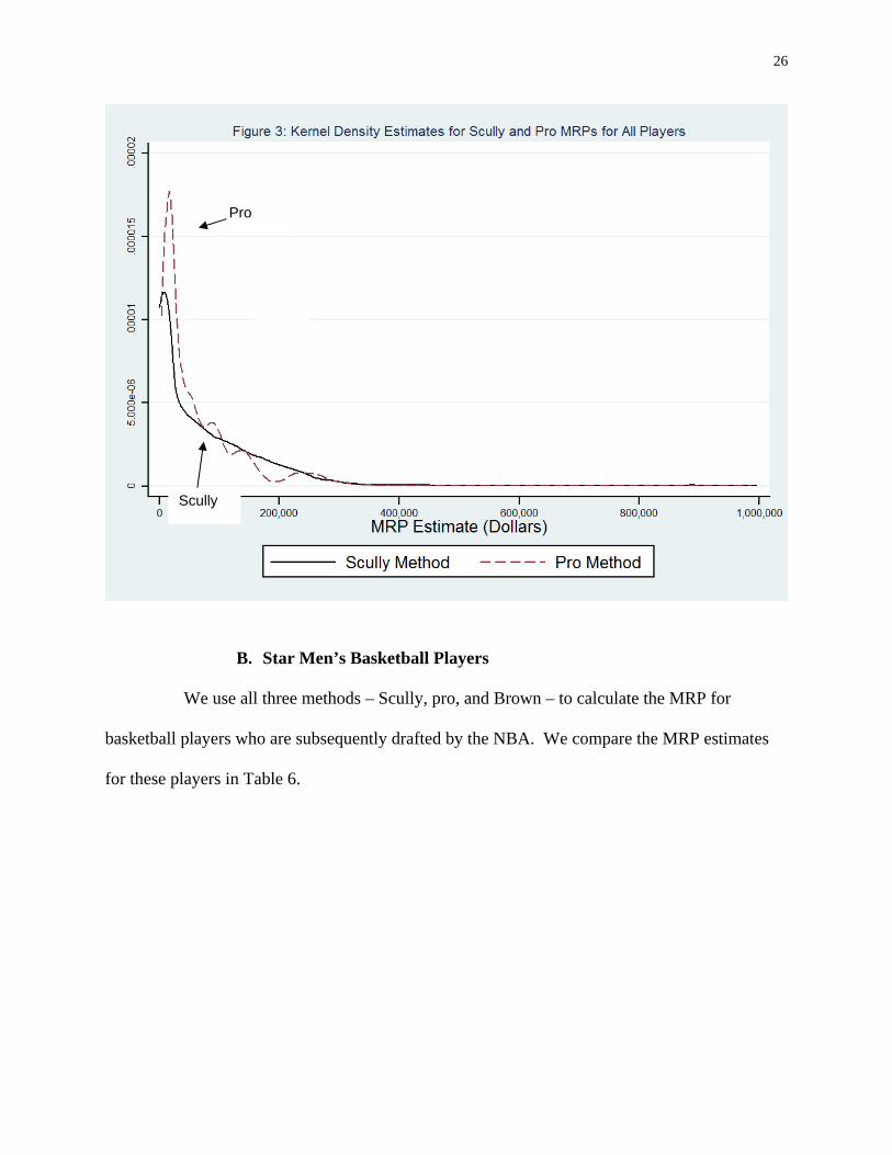
VI. Comparison of MRP Estimates

A. All Men’s Basketball Players

We are able to estimate MRPs for all men’s basketball players using the Scully method

and a variation incorporating information on the shape of the pro salary distribution. To

illustrate differences in the entire distribution of MRP estimates, we graph the kernel density of

the MRP estimates for the Scully and pro methods in Figure 3.36 From the graph, we can see

that the distribution of the Scully estimates are shifted leftwards (towards zero) relative to the pro

estimates.

35 The results for alternative definitions of large schools (i.e., schools with basketball revenues greater than $8, $9, $11, or $12 million) give similar results when fixed effects are excluded or included. 36 Kernel densities are constructed with a commonly used technique for smoothing density functions that would normally be portrayed in histograms. The smoothness of the kernel density function is inversely proportional to the width of the bandwidth being used. In our case, we use a bandwidth around MRP values of $10,000.

For legibility reasons, we limit the graphical presentation to only those MRP estimates that are less than $1 million. Over 95% of the MRPs are included in the graph. The two densities are largely coincident beyond $1 million, except that the density using the pro method is slightly higher than the Scully method for MRP estimates around $1.25 million.

26

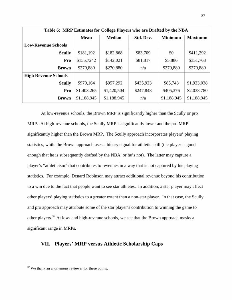
B. Star Men’s Basketball Players

We use all three methods – Scully, pro, and Brown – to calculate the MRP for

basketball players who are subsequently drafted by the NBA. We compare the MRP estimates

for these players in Table 6.

Scully

Pro

27

Table 6: MRP Estimates for College Players who are Drafted by the NBA

Mean Median Std. Dev. Minimum Maximum

Low-Revenue Schools

Scully $181,192 $182,868 $83,709 $0 $411,292

Pro $155,7242 $142,021 $81,817 $5,886 $351,763

Brown $270,880 $270,880 n/a $270,880 $270,880

High Revenue Schools

Scully $970,164 $957,292 $435,923 $85,748 $1,923,038

Pro $1,403,265 $1,420,504 $247,848 $405,376 $2,038,780

Brown $1,188,945 $1,188,945 n/a $1,188,945 $1,188,945

At low-revenue schools, the Brown MRP is significantly higher than the Scully or pro

MRP. At high-revenue schools, the Scully MRP is significantly lower and the pro MRP

significantly higher than the Brown MRP. The Scully approach incorporates players’ playing

statistics, while the Brown approach uses a binary signal for athletic skill (the player is good

enough that he is subsequently drafted by the NBA, or he’s not). The latter may capture a

player’s “athleticism” that contributes to revenues in a way that is not captured by his playing

statistics. For example, Denard Robinson may attract additional revenue beyond his contribution

to a win due to the fact that people want to see star athletes. In addition, a star player may affect

other players’ playing statistics to a greater extent than a non-star player. In that case, the Scully

and pro approach may attribute some of the star player’s contribution to winning the game to

other players.37 At low- and high-revenue schools, we see that the Brown approach masks a

significant range in MRPs.

VII. Players’ MRP versus Athletic Scholarship Caps

37 We thank an anonymous reviewer for these points.

28

We compare players’ MRPs, a lower bound on a player’s marginal contribution to a

school, with an upper bound on the athletic scholarship received by players.38 We are able to

compare MRPs to the original athletic scholarship cap (the GIA (grant-in-aid)), the new cap

(covering GIA plus up to $2,000for incidental expenses), and COA (proposed cap, covers total

estimated incidental expenses), for slightly more than 15,000 player-year combinations.

Recall that we do not observe the actual scholarship received by each student-athlete, but

we know the maximum scholarship received is equal to the cap. If the student-athlete’s MRP is

above his scholarship limit, then the MRP is also definitely above the actual scholarship received

by the student-athlete. Similarly, we cannot observe the full marginal value that the player

contributes to the school. The MRPs are underestimates of the marginal value of the student-

athlete to the schools, because they only capture the direct revenue impact.

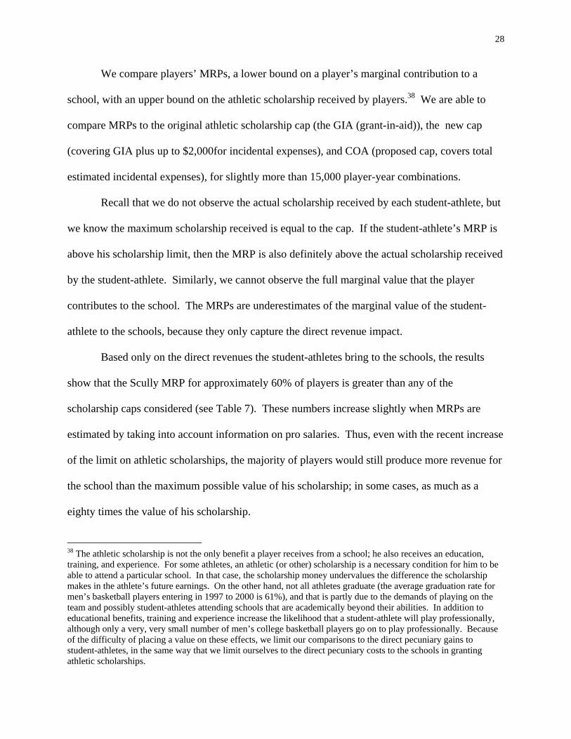
Based only on the direct revenues the student-athletes bring to the schools, the results

show that the Scully MRP for approximately 60% of players is greater than any of the

scholarship caps considered (see Table 7). These numbers increase slightly when MRPs are

estimated by taking into account information on pro salaries. Thus, even with the recent increase

of the limit on athletic scholarships, the majority of players would still produce more revenue for

the school than the maximum possible value of his scholarship; in some cases, as much as a

eighty times the value of his scholarship.

38 The athletic scholarship is not the only benefit a player receives from a school; he also receives an education, training, and experience. For some athletes, an athletic (or other) scholarship is a necessary condition for him to be able to attend a particular school. In that case, the scholarship money undervalues the difference the scholarship makes in the athlete’s future earnings. On the other hand, not all athletes graduate (the average graduation rate for men’s basketball players entering in 1997 to 2000 is 61%), and that is partly due to the demands of playing on the team and possibly student-athletes attending schools that are academically beyond their abilities. In addition to educational benefits, training and experience increase the likelihood that a student-athlete will play professionally, although only a very, very small number of men’s college basketball players go on to play professionally. Because of the difficulty of placing a value on these effects, we limit our comparisons to the direct pecuniary gains to student-athletes, in the same way that we limit ourselves to the direct pecuniary costs to the schools in granting athletic scholarships.

29

Table 7: Comparison of MRPs to Athletic Scholarship Limits

Estimating Method: Scully Pro

% of MRPs > GIA 58% 60%

% of MRPs > new cap 59% 61%

% of MRPs > COA 60% 63%

One explanation for the MRPs that are below the scholarship limit is that athletic

scholarships are set ex ante, before the season and hence based on a student-athlete’s expected

performance, while the estimates of MRPs are ex post, based on the student-athlete’s actual

performance. Thus, ex post a player’s MRP may be below his scholarship limit, while ex ante

his MRP is above a scholarship limit. While coaches adjust their expectations based on a

player’s high school record, suppose that the average MRP of current players is a reasonable

proxy for each player’s ex ante MRP. We find that the average MRP, our hypothetical proxy for

each player’s ex ante MRP, is above the original and current scholarship limit for every school in

our sample.

Finally, consider the MRP estimates for the college players who are ultimately drafted by

the NBA. Regardless of the method used to estimate drafted players’ MRPs, virtually all

estimates are greater than the player’s original or new cap on athletic scholarships.39 Thus, all

drafted players contribute more revenue to their school than they receive in athletic

scholarships.40 On average, the MRPs are over ten times greater than the GIA received by the

39 The exceptions are Joe Alexander at West Virginia and Dante Cunningham at Villanova, both based on freshman year only. 40 The question of whether college athletes generate more revenue than they receive in financial aid has been tackled before for men’s basketball players who are subsequently drafted by professional leagues. Brown, 1994, finds that star college men’s basketball players on average generate between $871,310 and $1,283,000, while he estimates the typical scholarship at roughly $20,000.

30

player. Based on the Scully method, the maximum difference is over fifty times greater than the

GIA.

VIII. Conclusion

We estimate MRPs based on the student-athlete’s playing statistics, as well as using a

variation that incorporates pro salary distribution data. We find that about 60% of men’s

basketball players have a monetary contribution to the school that is greater, often substantially

greater, than the value of the scholarship the player received. We conclude that most men’s

college basketball players are paid less – often substantially less – than their monetary benefit to

the college for which they play.

Second, we estimate MRPs for college players who are ultimately drafted by the NBA

based on a player’s performance statistics, incorporating the distribution of pro salaries, and by

directly estimating the effect of the presence of future drafted players on revenues earned by the

team. We find that virtually 100% of drafted players contribute more revenues to their school

than they receive in the form of scholarships; the degree to which schools “profit” from these star

players ranges from $7,000 to $1.8 million, with an average of about $400,000.

Finally, we compare the MRPs estimated using the different methods. For all men’s

basketball players, we find broadly similar results when using playing statistics whether or not

the distribution of pro salaries is incorporated. For drafted players, we find some difference in

the mean MRP similar across the three methods, although the mean MRPs are in the same

ballpark regardless of the method used to estimate MRP. The difference in the three methods is

more obvious in terms of the variation in MRPs. In particular, the Brown approach, by

construction, provides a single MRP estimate for all drafted players at low-revenue schools and a

second single MRP estimate for all drafted players at high-revenue schools, regardless of

31

position or quality of the player. The MRPs as estimated by the Scully and pro methods show a

range in estimated MRPs, from about $5,000 to over $400,000 at low-revenue schools and from

$100,000 to $2 million at high-revenue schools.

We have implemented three methods for measuring MRP. Each method gives somewhat

different numerical results, but the conclusion that stems from each one is the same: a majority

of men’s college basketball players contribute more to their schools’ revenue than what they get

from the schools.

32

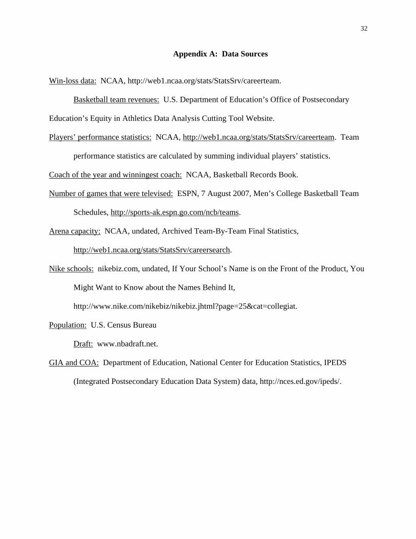
Appendix A: Data Sources

Win-loss data: NCAA, http://web1.ncaa.org/stats/StatsSrv/careerteam.

Basketball team revenues: U.S. Department of Education’s Office of Postsecondary

Education’s Equity in Athletics Data Analysis Cutting Tool Website.

Players’ performance statistics: NCAA, http://web1.ncaa.org/stats/StatsSrv/careerteam. Team

performance statistics are calculated by summing individual players’ statistics.

Coach of the year and winningest coach: NCAA, Basketball Records Book.

Number of games that were televised: ESPN, 7 August 2007, Men’s College Basketball Team

Schedules, http://sports-ak.espn.go.com/ncb/teams.

Arena capacity: NCAA, undated, Archived Team-By-Team Final Statistics,

http://web1.ncaa.org/stats/StatsSrv/careersearch.

Nike schools: nikebiz.com, undated, If Your School’s Name is on the Front of the Product, You

Might Want to Know about the Names Behind It,

http://www.nike.com/nikebiz/nikebiz.jhtml?page=25&cat=collegiat.

Population: U.S. Census Bureau

Draft: www.nbadraft.net.

GIA and COA: Department of Education, National Center for Education Statistics, IPEDS

(Integrated Postsecondary Education Data System) data, http://nces.ed.gov/ipeds/.

33

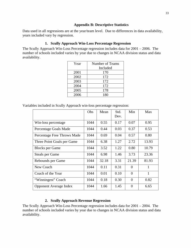
Appendix B: Descriptive Statistics Data used in all regressions are at the year/team level. Due to differences in data availability, years included vary by regression.

1. Scully Approach Win-Loss Percentage Regression The Scully Approach Win-Loss Percentage regression includes data for 2001 – 2006. The number of schools included varies by year due to changes in NCAA division status and data availability.

Year Number of Teams Included

2001 170 2002 172 2003 172 2004 172 2005 178 2006 180

Variables included in Scully Approach win-loss percentage regression:

Obs Mean Std. Dev.

Min Max

Win-loss percentage 1044 0.55 0.17 0.07 0.95

Percentage Goals Made 1044 0.44 0.03 0.37 0.53

Percentage Free Throws Made 1044 0.69 0.04 0.57 0.80

Three Point Goals per Game 1044 6.38 1.27 2.72 13.93

Blocks per Game 1044 3.52 1.22 0.80 10.79

Steals per Game 1044 6.98 1.46 3.73 23.36

Rebounds per Game 1044 32.18 3.31 21.39 81.93

New Coach 1044 0.11 0.31 0 1

Coach of the Year 1044 0.01 0.10 0 1

“Winningest” Coach 1044 0.18 0.30 0 0.82

Opponent Average Index 1044 1.66 1.45 0 6.65

2. Scully Approach Revenue Regression The Scully Approach Win-Loss Percentage regression includes data for 2001 – 2004. The number of schools included varies by year due to changes in NCAA division status and data availability.

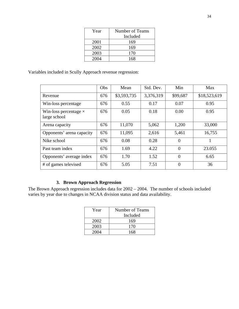
34

Year Number of Teams Included

2001 169 2002 169 2003 170 2004 168

Variables included in Scully Approach revenue regression:

Obs Mean Std. Dev. Min Max

Revenue 676 $3,593,735 3,376,319 $99,687 $18,523,619

Win-loss percentage 676 0.55 0.17 0.07 0.95

Win-loss percentage × large school

676 0.05 0.18 0.00 0.95

Arena capacity 676 11,070 5,062 1,200 33,000

Opponents’ arena capacity 676 11,095 2,616 5,461 16,755

Nike school 676 0.08 0.28 0 1

Past team index 676 1.69 4.22 0 23.055

Opponents’ average index 676 1.70 1.52 0 6.65

# of games televised 676 5.05 7.51 0 36

3. Brown Approach Regression The Brown Approach regression includes data for 2002 – 2004. The number of schools included varies by year due to changes in NCAA division status and data availability.

Year Number of Teams Included

2002 169 2003 170 2004 168

35

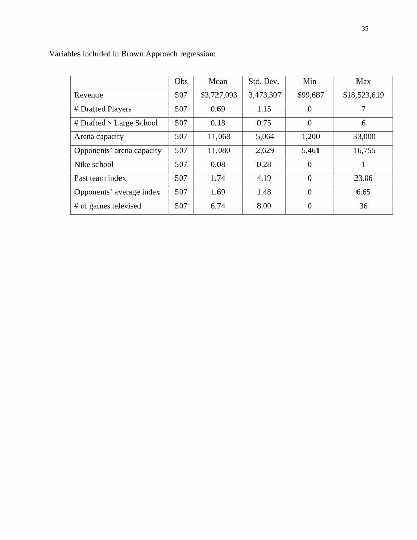
Variables included in Brown Approach regression:

Obs Mean Std. Dev. Min Max

Revenue 507 $3,727,093 3,473,307 $99,687 $18,523,619

# Drafted Players 507 0.69 1.15 0 7

# Drafted × Large School 507 0.18 0.75 0 6

Arena capacity 507 11,068 5,064 1,200 33,000

Opponents’ arena capacity 507 11,080 2,629 5,461 16,755

Nike school 507 0.08 0.28 0 1

Past team index 507 1.74 4.19 0 23.06

Opponents’ average index 507 1.69 1.48 0 6.65

# of games televised 507 6.74 8.00 0 36

36

References Berri, David J., December 1999, “Who is ‘Most Valuable’? Measuring the Player’s

Production of Wins in the National Basketball Association”, Managerial and Decision

Economics, Vol. 20(8), pp. 411-427.

Bradbury, John Charles, December 2007, “Does the Baseball Labor Market Properly

Value Pitchers?”, Journal of Sports Economics, Vol. 8(6), pp. 616-632.

Brown, Robert, October 1993, “An Estimate of the Rent Generated by a Premium

College Football Player”, Economic Inquiry, Vol. XXXI, pp. 671-684.

Brown, Robert, 1994, “Measuring Cartel Rents in the College Basketball Player

Recruitment Market”, Applied Economics, Vol. 26, pp. 27-34.

Brown, Robert, April 2011, “Research Note: Estimates of College Football Player

Rents”, Journal of Sports Economics, Vol. 12(2), pp. 200-212.Chatterjee, Sangit and Martin R.

Campbell, 1994, “Take That Jam! An Analysis of Winning Percentage for NBA Teams”,

Managerial and Decision Economics, Vol. 15, pp. 521-535.

Hadley, Lawrence, et. al., March 2000, “Performance Evaluation of National Football

League Teams”, Managerial and Decision Economics, Vol. 21(2), pp. 63-70.

Hill, J. Richard and Peter A. Groothuis, May 2001, “The New NBA Collective

Bargaining Agreement, the Median Voter Model, and a Robin Hood Rent Redistribution”,

Journal of Sports Economics, Vol. 2(2), pp. 131-144.

Hofler, Richard A. and James E. Payne, 1997, “Measuring Efficiency in the National

Basketball Association”, Economics Letters, Vol. 55, pp. 293-299.

Krautmann, Anthony C., April 1999, “What's Wrong with Scully-Estimates of a Player’s

Marginal Revenue Product”, Economic Inquiry, Vol. 37(2), pp. 369-381.

37

Leonard, John and Joseph Prinzinger, 1984, “An Investigation into the Monopsonistic

Market Structure of Division One NCAA Football and its Effect on College Football Players”,

Eastern Economic Journal, Vol. 10(4), pp. 455-467.

Martin, Robert E., April 2004, “Tuition Discounting Without Tears”, Economics of

Education Review, Vol. 23(2), pp. 177-189.

Staudohar, P., April 1999, “Labor Relations in Basketball: The Lockout of 1988-99”,

Monthly Labor Review, U.S. Department of Labor, pp. 3-9.

Scott, Frank A., James E. Long, and Ken Somppi, September 1985, “Salary vs. Marginal

Revenue Product Under Monopsony and Competition: The Case of Professional Basketball”,

Atlantic Economic Journal, Vol. 13:3, pp. 50-59.

Scully, Gerald W., December 1974, “Pay and Performance in Major League Baseball”,

The American Economic Review, Vol. 64 (6), pp. 915-930.

Zak, Thomas A., Cliff J. Huang and John J. Siegfried, 1979, “Production Efficiency: The

Case of Professional Basketball”, Journal of Business, Vol. 52(3), pp. 379-392.

Zimbalist, Andrew (1999). Unpaid Professionals: Commercialism and Conflict in Big

Time Sports, p. 138, Princeton University Press, Princeton, NJ.

38

Notes